Lab Report 2a

KNS 2591 Civil Engineering Laboratory 3 Faculty of Engineering Universiti Malaysia Sarawak

____________________________________________________________ TITLE:

L2a – Sieve Analysis

INTRODUCTION:

The range of particle size encountered in soils is very wide; from around

200mm down to the colloidal size of some clays of less than 0.001 mm. although

the natural soils are mixtures of various-sized particles, it is common to find a

predominance occurring within a relatively narrow band of sizes. When the width

of this size band is very narrow, the soil will be termed poorly graded, if it is wide

then the soil is said to be well graded. A number of engineering properties e.g.

permeability, frost susceptibility, compressibility, are related directly or indirectly

to particle-size characteristics.

The particle-size analysis of a soil is carried out by determining the weight

percentages falling within bands of size represented by the divisions and

subdivisions of British Standard range of particle size. One of them is sieve

analysis, which is a practice or procedure are use to assess the particle size

distribution of granular material. The size distribution is often of critical

importance to the way the material performs in use. A sieve analysis can be

performed on any type of non-organic or organic granular materials including

sands, crushed rock, clays, granite, coal, soils, a wide range of manufactured

powders, grain and seeds, down to a minimum size depending on the exact

method. Being such a simple technique of particle sizing, it is probably the most

common.

THEORY:

Particle size analysis and grading

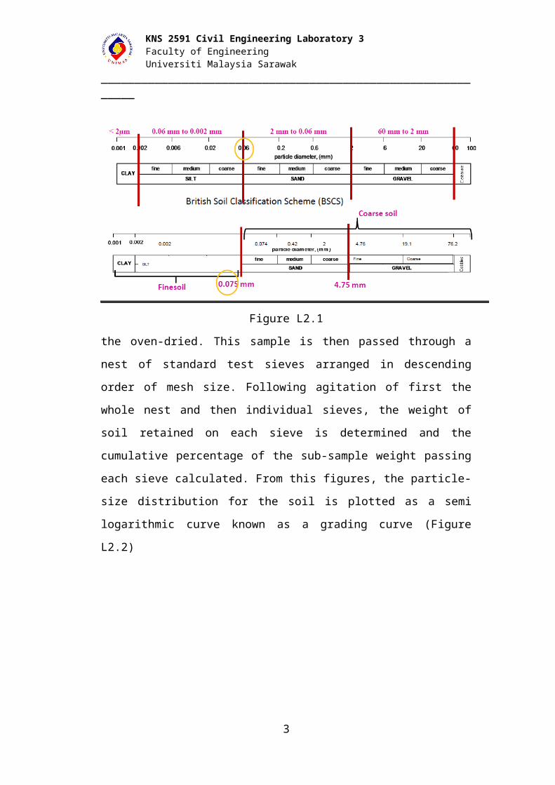
As stated before, the particle-size analysis of a soil is carried out by

determining the weight percentages falling within bands of size represented by

divisions and sub-divisions, which is called as British Standard range of particle

sizes (Figure L2.1). In the case of a coarse soil, from which fine-grained particles

have been removed or were absent, the usual process is a sieve analysis. A

1


____________________________________________________________ representative sample of the soil is split systematically down to a convenient sub-

sample size and

Figure L2.1

the oven-dried. This sample is then passed through a nest of standard test sieves

arranged in descending order of mesh size. Following agitation of first the whole

nest and then individual sieves, the weight of soil retained on each sieve is

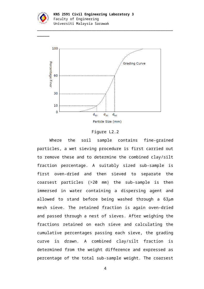
determined and the cumulative percentage of the sub-sample weight passing each

sieve calculated. From this figures, the particle-size distribution for the soil is

plotted as a semi logarithmic curve known as a grading curve (Figure L2.2)

Figure L2.2

2


____________________________________________________________

Where the soil sample contains fine-grained particles, a wet sieving

procedure is first carried out to remove these and to determine the combined

clay/silt fraction percentage. A suitably sized sub-sample is first oven-dried and

then sieved to separate the coarsest particles (>20 mm) the sub-sample is then

immersed in water containing a dispersing agent and allowed to stand before

being washed through a 63μm mesh sieve. The retained fraction is again oven-

dried and passed through a nest of sieves. After weighing the fractions retained on

each sieve and calculating the cumulative percentages passing each sieve, the

grading curve is drawn. A combined clay/silt fraction is determined from the

weight difference and expressed as percentage of the total sub-sample weight. The

coarsest fraction can also be sieved and the results used to complete the grading

curve.

Grading characteristics

The grading curve is a graphical representation of the particle-size

distribution and is therefore useful in itself as a means of describing the oil. For

this reason it is always a good idea to include copies of grading curves in

laboratory and other similar reports. It should also be remembered that the

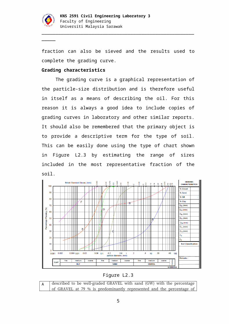
primary object is to provide a descriptive term for the type of soil. This can be

easily done using the type of chart shown in Figure L2.3 by estimating the range

of sizes included in the most representative fraction of the soil.

Figure L2.3

3


____________________________________________________________ A described to be well-graded GRAVEL with sand (GW) with the percentage of GRAVEL at

79 % is predominantly represented and the percentage of SAND is more than 15 %

B described to be silty SAND with gravel (SM) with the percentage of SAND is predominant

at 60 % with gravel is more than 15 % and silt at 10 %

C described as poorly-graded SAND (SP) as the percentage of SAND lies in the medium

range is 75 %

D described as poorly-graded SAND with silt (SP-SM) with the percentage of SAND lies in

the fine range of 85 % and silt is at 15 %

E described to be sandy SILT (ML) as SILT is predominant at 60 % with sand encountered at

30 %

F described to be silty CLAY (CL-ML) as the clay percentage is dominant at 55 % and silt is

at 45 %

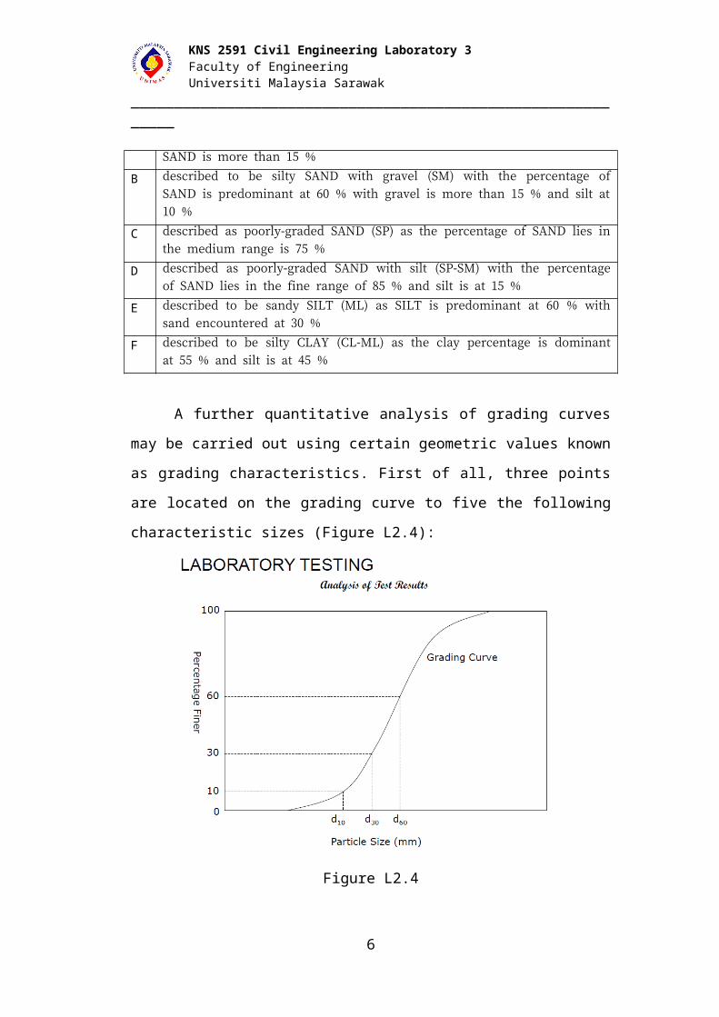
A further quantitative analysis of grading curves may be carried out using

certain geometric values known as grading characteristics. First of all, three points

are located on the grading curve to five the following characteristic sizes (Figure

L2.4):

Figure L2.4

d10 – maximum size of the smallest 10% of the sample



4


____________________________________________________________

from these characteristic sizes, the following grading characteristics are defined :

Effective Size = d10 mm

Coefficient of uniformity, Cu

Coefficient of Curvature / Gradation, Cc

Both Cu and Cc will be unity (equal to 1) for a single-sized soil, while Cu < 3

indicating uniform grading and Cu > 3 for well-graded soil

Most well graded soil will have grading curves that are mainly flat of

slightly concave, giving values of Cc between o.5 and 2.0. One useful application

is an approximation of the coefficient of permeability, which was suggested by

Hazen.

OBJECTIVE:

The objective of this test is to determine the grain size distribution of soil by sieve

analysis.

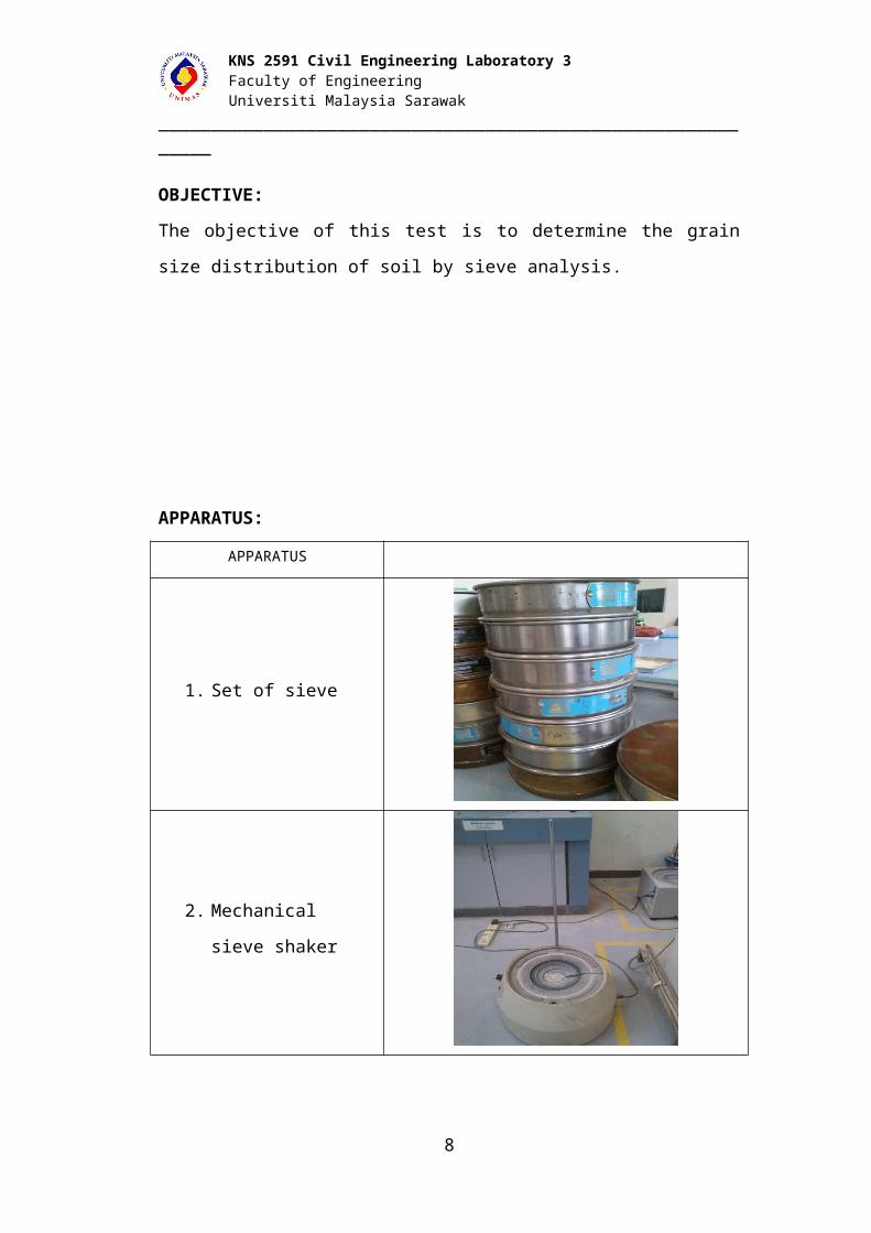
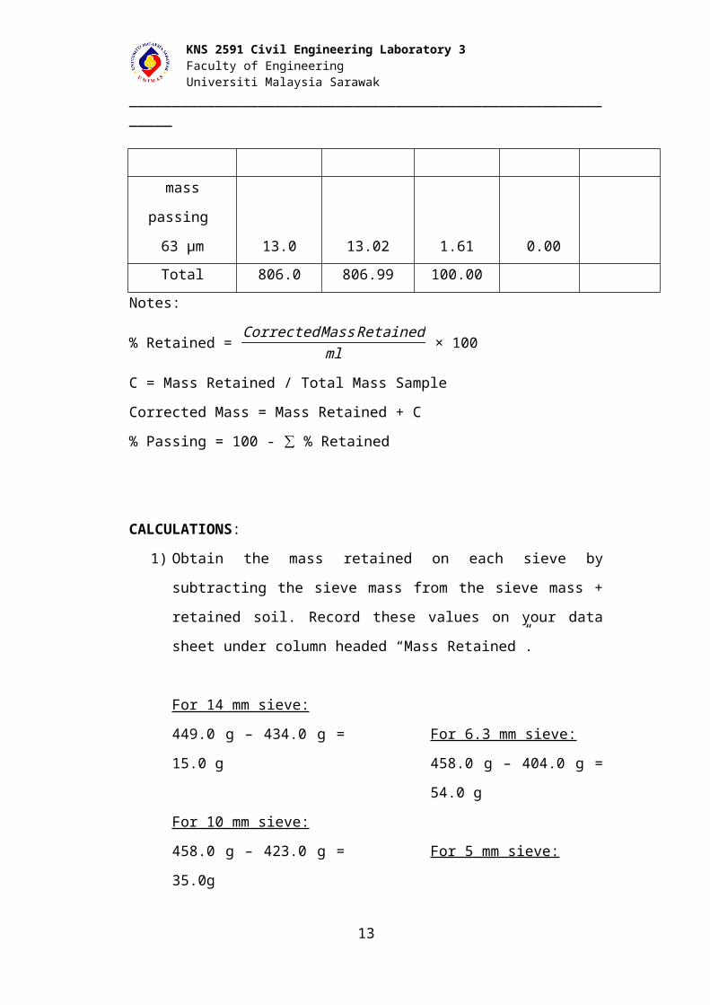
APPARATUS:

APPARATUS

5

Cu=D60

D10

Cc=( D30)2

( D10×D60 )


____________________________________________________________

1. Set of sieve

2. Mechanical sieve

shaker

PROCEDURE:

1. 806g air-dried coarse-grained soil sample was taken and was recorded on

data sheet. The sieve was set in order from pan to lid.

6


____________________________________________________________

Size of Sieve

14 mm

10 mm

6.3 mm

5 mm

3.35 mm

2 mm

1.18 mm

600 µm

425 µm

300 µm

212 µm

150 µm

63 µm

Pan

2. The sieve was cleaned first by using the brush to remove the particle from

the screen. After the sieve was cleaned and stacked on order, the sample

was poured onto the upper sieve and closed the sieve using the lid.

3. The stack of the sieve was placed at mechanical sieve shaker and was

shaken for 10 minute. After that, the stack of sieve was removed one by

one from the shaker and each sieve was weighed to the nearest 0.1g and

was recorded inside the tabulation data sheet.

4. The mass retained on each sieve was obtained by subtracting the sieve

mass from the sieve mass + retained soil. This mass was recorded inside

the tabulation data sheet.

5. Various equations were used in order to complete this calculation for this

experiment. Some of them were:

a. % Retained = Corrected Mass Retained

ml × 100

b. C = Mass Retained / Total Mass Sample

c. Corrected Mass = Mass Retained + C

d. % Passing = 100 - ∑ % Retained

7


____________________________________________________________

6. The graph of percentage finer against particle size was plotted.

RESULT

Preparation

Dried Sample + Tray (g) 910

Tray (g) 104

8


____________________________________________________________ Dried Sample (g) 806

BS Test

Sieve

Mass

Retained (g)

Corrected

Mass (g)

%

Retained

%

Passing

Max Load

(g)

14 mm 15.0 15.02 1.86 98.14 1500

10 mm 35.0 35.04 4.34 93.80 1000

6.3 mm 54.0 54.07 6.70 87.10 750

5mm 27.0 27.03 3.35 83.75 500

3.35 mm 50.0 50.06 6.20 77.55 400

2.36mm 25.0 25.03 3.10 74.45 250

1.18 mm 52.0 52.06 6.45 68.00 100

600 µm 104.0 104.13 12.90 55.10 75

425 µm 100.0 100.12 12.41 42.69 75

300 µm 115.0 115.14 14.27 28.42 50

212 µm 73.0 73.09 9.06 19.36 50

150 µm 61.0 61.08 7.57 11.79 40

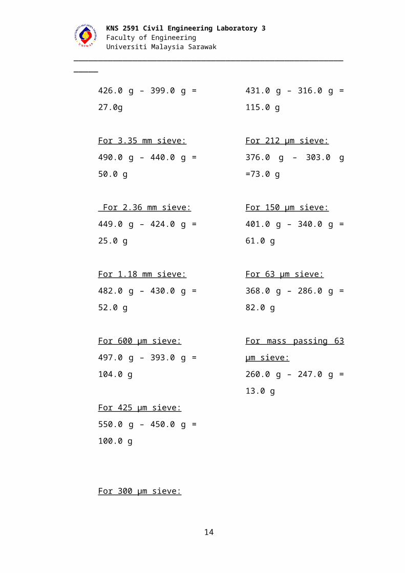
63 µm 82.0 82.10 10.18 1.61 25

mass passing

63 µm 13.0 13.02 1.61 0.00

Total 806.0 806.99 100.00

Notes:

% Retained = Corrected Mass Retained

ml × 100

C = Mass Retained / Total Mass Sample

Corrected Mass = Mass Retained + C

% Passing = 100 - ∑ % Retained

CALCULATIONS:

1) Obtain the mass retained on each sieve by subtracting the sieve mass from

the sieve mass + retained soil. Record these values on your data sheet

under column headed “Mass Retained”.

9


____________________________________________________________

For 14 mm sieve:

449.0 g – 434.0 g = 15.0 g

For 10 mm sieve:

458.0 g – 423.0 g = 35.0g

For 6.3 mm sieve:

458.0 g – 404.0 g = 54.0 g

For 5 mm sieve:

426.0 g – 399.0 g = 27.0g

For 3.35 mm sieve:

490.0 g – 440.0 g = 50.0 g

For 2.36 mm sieve:

449.0 g – 424.0 g = 25.0 g

For 1.18 mm sieve:

482.0 g – 430.0 g = 52.0 g

For 600 µm sieve:

497.0 g – 393.0 g = 104.0 g

For 425 µm sieve:

550.0 g – 450.0 g = 100.0 g

For 300 µm sieve:

431.0 g – 316.0 g = 115.0 g

For 212 µm sieve:

376.0 g – 303.0 g =73.0 g

For 150 µm sieve:

401.0 g – 340.0 g = 61.0 g

For 63 µm sieve:

368.0 g – 286.0 g = 82.0 g

For mass passing 63 µm

sieve:

260.0 g – 247.0 g = 13.0 g

10


____________________________________________________________

2) Now sum this column of masses (including that in the pan) and compare

with the mass obtained.

Total mass retained = (15.0 + 35.0 + 54.0 + 27.0 + 50.0 + 25.0 + 52.0 +

104.0 + 100.0 + 115.0 + 73.0 + 61.0 + 82.0 + 13.0)

g

= 806.0g

The mass obtained is the same with the mass retained, which is 806.0g.

3) Compute the percent retained on each sieve by dividing the weight

retained on each sieve by the original sample mass. This is valid, since any

material passing the No. 200 sieve will pass any sieve above it in the stack.

For 14 mm sieve:

% Retained = (15.02/806.99) x

100%

= 1.86 %

For 10 mm sieve:

% Retained = (35.04/806.99) x

100%

= 4.34%

For 6.3 mm sieve:

% Retained = (54.07/806.99) x

100%

= 6.70 %

For 5mm sieve:

% Retained = (27.03/806.99) x

100%

= 3.35 %

For 3.35 mm sieve:

% Retained = (50.06/806.99) x

100%

= 6.20 %

For 2.36 mm sieve:

% Retained = (25.03/806.99) x

100%

= 3.10 %

For 1.18 mm sieve:

% Retained = (52.06/806.99) x

100%

= 6.45 %

For 600 µm sieve:

% Retained = (104.13/806.99) x

100%

= 12.90%

For 425 µm sieve:

% Retained = (100.12/806.99) x

100%

= 12.41 %

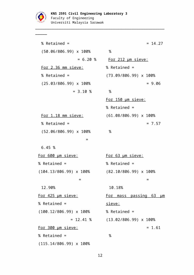
For 300 µm sieve:

11


____________________________________________________________

% Retained = (115.14/806.99) x

100%

= 14.27 %

For 212 µm sieve:

% Retained = (73.09/806.99) x 100%

= 9.06 %

For 150 µm sieve:

% Retained = (61.08/806.99) x 100%

= 7.57 %

For 63 µm sieve:

% Retained = (82.10/806.99) x 100%

= 10.18%

For mass passing 63 µm sieve:

% Retained = (13.02/806.99) x 100%

= 1.61 %

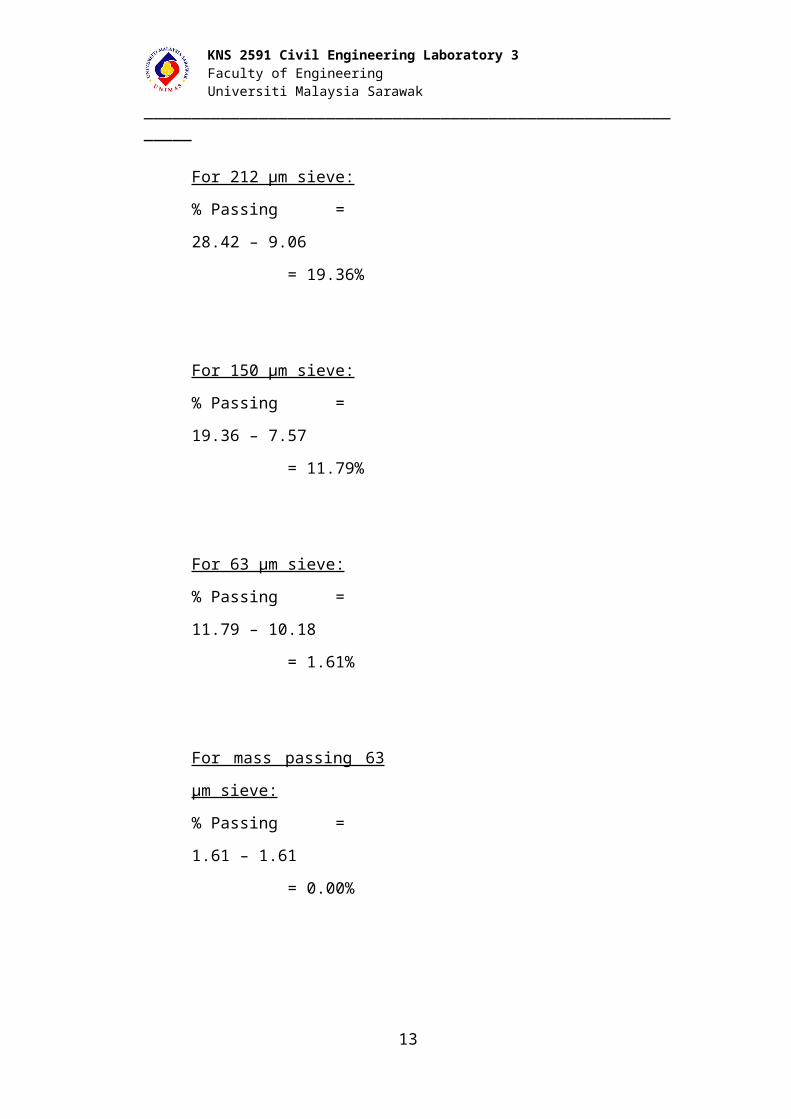
4) Compute the percent passing (or percent finer) by starting with 100

percent and subtracting the percent retained on each sieve as a cumulative

procedure.

12


____________________________________________________________ For 14 mm sieve:

% Passing = 100.00 –1.86

= 98.14%

For 10 mm sieve:

% Passing = 98.14 – 4.34

= 93.80%

For 6.3 mm sieve:

% Passing = 93.80 – 6.70

= 87.10%

For 5 mm sieve:

% Passing = 87.10 – 3.35

= 83.75%

For 3.35 mm sieve:

% Passing = 83.75 – 6.20

= 77.55%

For 2.36 mm sieve:

% Passing = 77.55 – 3.10

= 74.45%

For 1.18 mm sieve:

% Passing = 74.45 – 6.45

= 68.00%

For 600 µm sieve:

% Passing = 68.00 –

12.90

= 55.10%

For 425 µm sieve:

% Passing = 55.10 –

12.41

= 42.69%

For 300 µm sieve:

% Passing = 42.69 –

14.27

= 28.42%

For 212 µm sieve:

% Passing = 28.42 – 9.06

= 19.36%

For 150 µm sieve:

% Passing = 19.36 – 7.57

= 11.79%

For 63 µm sieve:

% Passing = 11.79 –

10.18

= 1.61%

For mass passing 63 µm

sieve:

% Passing = 1.61 – 1.61

= 0.00%

13


____________________________________________________________5) Each individual should make a semi logarithmic plot of particle size versus

percent finer, using the graph on the data sheet. If less than 12 percent

passes The No.200 sieve, compute CU and Cc and show on the graph.

1 10 1000

20

40

60

80

100

120

Particle size, mm

Perc

enta

ge fi

ner,

%

A graph of percentage finer against particle size

14


____________________________________________________________

Coefficient of Uniformity Cu

15


____________________________________________________________This is the indicator of the spread of the range of the grain sizes and is defined as

¿ 0.77mm0.13mm

Cu = 5.92

Coefficient of Curvature Cc

This is the measure of the shape of curve between D60 and D10 grain sizes,

defined as

Cc ¿(0.31)2

(0.13)(0.77)

Cc = 0.96

16

Cu=D60

D10

Cc=( D30)2

( D10×D60 )


____________________________________________________________DISCUSSION:

1. The grain-size distribution of coarse-grained soils, gravelly and/or

sandy, is usually determined by sieve analysis. Oven-dried soil with

the lumps thoroughly broken down is passed through a number of

sieves. The weight of the dry soil retained on each sieve is determined,

and based on these weights the cumulative percent passing a given

sieve is determined. This is generally referred to as percent finer.

2. The grain-size distribution can be used to determine some of the basic

soil parameters such as the effective size, the uniformity coefficient,

and the coefficient of gradation.

3. Thus, in this experiment, mass retained on each sieve is given below.

Sieve Size Mass Retained

14 mm 15.0 g

10 mm 35.0 g

6.3 mm 54.0 g

5 mm 27.0 g

3.35 mm 50.0 g

2.36 mm 25.0 g

1.18 mm 52.0 g

600 μm 104.0 g

425 μm 100.0 g

300 μm 115.0 g

212 μm 73.0 g

150 μm 61.0 g

63 μm 82.0 g

Passing 63μm 13.0 g

And, the total mass retained is 806.0 g.

4. Furthermore, percent retained on each sieve in this experiment is

computed below.

Sieve Size Percent Retained

17


____________________________________________________________14 mm 1.86 %

10 mm 4.34 %

6.3 mm 6.70 %

5 mm 3.35 %

3.35 mm 6.20 %

2.36 mm 3.10 %

1.18 mm 6.45 %

600 μm 12.90 %

425 μm 12.41%

300 μm 14.27 %

212 μm 9.06 %

150 μm 7.57 %

63 μm 10.18 %

Passing 63μm 1.61 %

5. Meanwhile, percent passing or percent finer in this experiment is

calculated as shown.

Sieve Size Percent Finer

14 mm 98.14 %

10 mm 93.80 %

6.3 mm 87.10 %

5 mm 83.75 %

3.35 mm 77.55 %

2.36 mm 74.45 %

1.18 mm 68.00 %

600 μm 55.10 %

425 μm 42.69 %

300 μm 28.42 %

212 μm 19.36 %

150 μm 11.79 %

63 μm 1.61 %

Passing 63μm 0 %

6. Grading curve is drawn by using Passing Finer (Percent Finer) as its y-

axis while Particle Size as its x-axis.

18


____________________________________________________________7. In this curve, we can get its effective size, diameter through which 10

% of the total soil mass is passing and is referred to as D10. The

uniformity coefficient, Cu is defined as

Cu=D60

D10

where D60 is the diameter through which 60% of the total soil mass is

passing. Hence, the value of Cu in this experiment is 5.92. In addition,

the coefficient of gradation C c is defined as

C c=(D30)

2

(D60)(D 10)

where D30 is the diameter through which 30% of the total soil mass is

passing, which is, the value of C c is 0.96.

8. A soil is called a well-graded soil if the distribution of the grain sizes

extends over a rather large range. In that case, the value of the

uniformity coefficient is large. Generally, a soil is referred to as well

graded if Cu is larger than C c.

9. When most of the grains in a soil mass are of approximately the same

size, the soil is called as poorly graded. A soil might have a

combination of two or more well-graded soil fractions, and this type of

soil is referred to as a gap-graded soil.

CONCLUSION:

In the conclusion, the soil is classified as gap-graded fine SAND soil. This

is due to the amount of sand is exceed 50 % (78.4%), while gravel and silt/clay

both at 18% and 3.6% respectively. For this curve, we obtained effective size of

19


____________________________________________________________0.13 mm. The value of uniformity coefficient and coefficient of curvature are 5.92

and 0.96 respectively.

There are few precaution need to be taken in order to get an accurate

result. There are:

Make sure that the sieve mesh is clean without any foreign soil/ items

stuck between them.

While shaking the sieve, make sure that the sieve was tighten properly so

that it can be sieved appropriately.

While taking reading on weight balance, make sure that there’s no zero

error occurred

RECOMMENDATION:

The experiment should be done carefully. The errors that we get from this

experiment are caused by instrumental and human errors.. However, instrumental

errors can be eliminated or minimized by carefully manipulation of apparatus.

This can be done by:

1. Make sure that the sieve mesh is clean without any foreign soil/ items

stuck between them

2. While shaking the sieve, make sure that the sieve was tighten properly so

that it can be sieved appropriately.

3. While taking reading on weight balance, make sure that there’s no zero

error occurred

Human errors can be minimized by doing the experiment carefully and

with intention to get the most accurate results possible.

REFERENCE:

Das, B. M., (1983). Advanced Soil Mechanics. Singapore : McGraw-Hill

International Editions.

20


____________________________________________________________

Roy Whitlow (2004), Basic Soil Mechanics (4th Ed.): Pearson Education Prentice

Hall

21

Documents

Lab Report 2a