Lab 7: Tables Operations in ArcGIS - giscourses.cfans.umn.edu · GIS Fundamentals Lab 7 Table Operations 1 Lab 7: Tables Operations in ArcGIS What You’ll Learn: This Lab provides

GIS Fundamentals Lab 7 Table Operations

1

Lab 7: Tables Operations in ArcGIS

What You’ll Learn: This Lab provides more practice with tabular data management in ArcGIS. In this Lab, we will view, select, re-order, and update tabular data. You should read chapter 8 in the GIS Fundamentals textbook before performing this Lab. Data: are in the \Lab7 directory, with census data USCounties.shp in a continental Albers projection, and soils.shp in UTM Zone 17, NAD83 meters coordinates. (note make sure you have the most current version of USCounties.shp. {An incomplete version of

USCounties.shp was initially placed in the \Lab7 directory and if you downloaded all folders at the start of class, you may have the wrong version. If you have incorrect version, re-download the \Lab7 data folder. The correct version has a date of 10/8/2018.}

What You’ll Produce: Three maps, two of selections based on census data, and one of a soils data set. You’ll also produce a table of soil properties. Background: Most spatial data in a GIS consist of at least two types of data, those data depicting the location and shape of objects, and text or numerical data describing the objects. These text and numerical data are most often contained in tables, and most GIS packages have some way of creating and editing these data tables. ArcGIS - provides a rich set of tools for viewing and displaying attribute data. However, you don’t have as many options for manipulating and saving table data, as with a full-featured database manager, so we’ll do some rather simple operations in this lab. Select by Attribute Last week we selected rows manually, by combinations of clicks and shift clicks on sorted rows. While sometimes this is the fastest and easiest way to select a set of features, more often we use a more complex query to select features. We’ll do some selections using a query builder. Start ArcGIS, and Add the data layer USCounties.shp to a new, empty project. Open the Attribute Table and review the table headings. Most of the headings are somewhat descriptive and describe statistics from the decadal U.S. Census for a period near the year 2000. These were pulled from various collaborating federal organizations, and include population, and crime. These data were all collected for county areas and referenced with a combined state-county FIPS code, which is unique for every state/county combination.


2

For example, POP2000 is the county population estimate for the year 2000, Med_Age is the median age of the county population, BURG01 is the number of reported burglaries for 2001, CropAcres is the number of acres of cultivated cropland in the county, and Cows the total number of bovine livestock in the county. Make a few practice maps that you don’t need to turn in, to get to know the data, e.g., Median age by county, from 31.7 (brown) to 54.3 (red):


3

Or population per density from low (brown) to high (red):

Let’s take a look at burglary rates. First create a map that displays burglaries for each county, in the variable BURG01, using a Quantile color distribution with 10 classes: Note a couple of things, that the counties with the highest populations have the highest number, and that there is probably something amiss on the reporting for less populous counties in Illinois and Kentucky. As with many statistics, the burglaries should be normalized by total population. As shown earlier, we do this by adding a field via a displayed table, then giving it a name and type in the Fields table: (remember to Save in the top Fields ribbon menu)


4

We can then activate the table display, and right click on the new column to invoke the Calculate Field tool (right):

We can then build our expression as shown in last week’s lab, selecting the target variable (top arrow at left), fields and operators (middle two arrows), to form an assignment equation (bottom arrow). Clicking on Run should apply the equation to calculate the burglary rate as a number per 100 persons per year.

Your display should look something like the image at right if you use a quantile class distribution with 10 classes. A quick look at the statistics for burglary rate show a 90th percentile at 1.037 burglaries per 100 people. If we wish to select the counties that have these higher rates, we could do this with a manual selection, but it is a lot of counties to scroll through, so we’ll build a query instead.


5

When you displayed the table, a Table View group appeared along the top ribbon of the main window. Find it, and then click on the Select by Attributes tool (see figure at right). we can query the data via the Select by Attributes tool: This opens a Geoprocessing Pane on the right side of the main window, in which you enter the target data layer or table, and the type of selection. You may create a new selection, meaning start from scratch with the table with no data currently selected. You may also choose various other kinds of selections, for example, those that add to, subtract from, or do other things with a currently selected set of records and perhaps additional records. Let’s create a query. Click on the Add Clause button, and it should display a clause builder:

You build the clause by populating each of the windows, through a combination of selections from dropdowns, and from typing values, as needed.


6

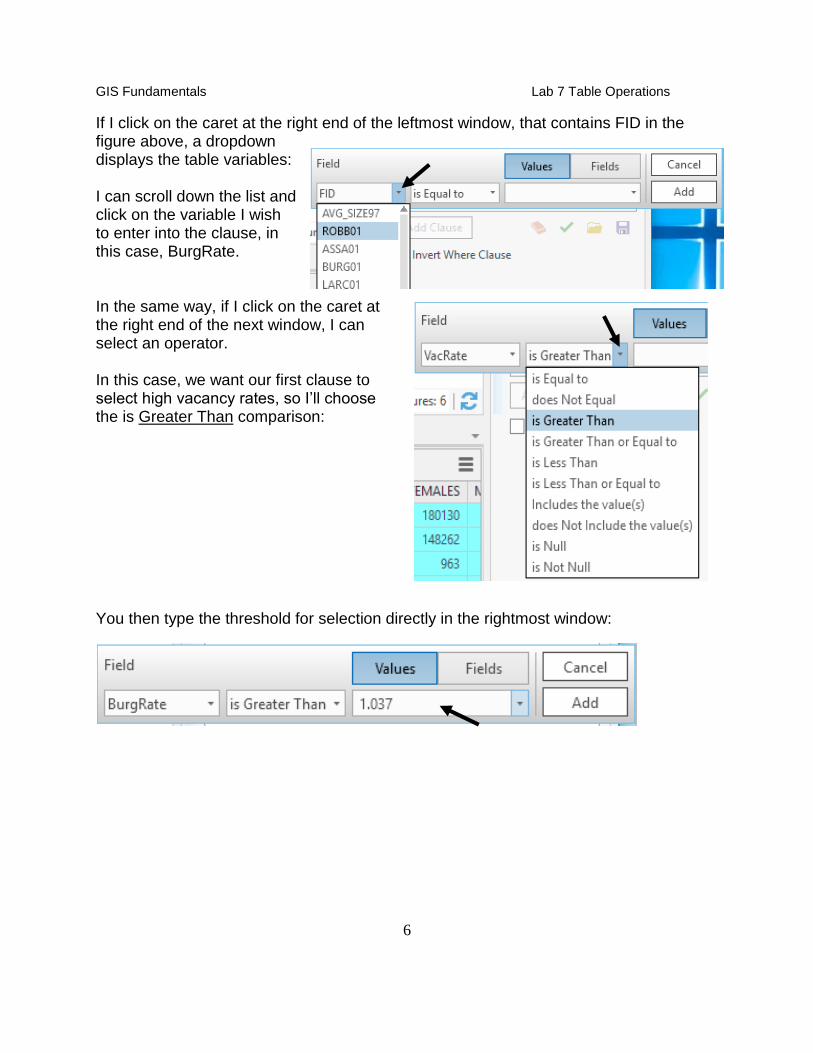
If I click on the caret at the right end of the leftmost window, that contains FID in the figure above, a dropdown displays the table variables: I can scroll down the list and click on the variable I wish to enter into the clause, in this case, BurgRate. In the same way, if I click on the caret at the right end of the next window, I can select an operator. In this case, we want our first clause to select high vacancy rates, so I’ll choose the is Greater Than comparison: You then type the threshold for selection directly in the rightmost window:


7

Add it to the query list by clicking on Add on the query bar (see above), and then Run near the bottom right of the Geoprocessing Pane displaying the query tool. This should display a set of selected counties as on the right: Note if you open the table, some of the selected polygons will show with the rows in the selection color, while unselected will not (see at right): You can toggle between showing all records in the table and showing only selected records in the table by clicking on the two icons displayed near the lower left corner of the table:

Again, data are collected by state agencies for most states, so variation in methods and definitions between states can lead to odd differences at state boundaries. The simplest comparisons are within state, although cross state differences can be conducted with proper adjustments.

Display All

Display only selected records


8

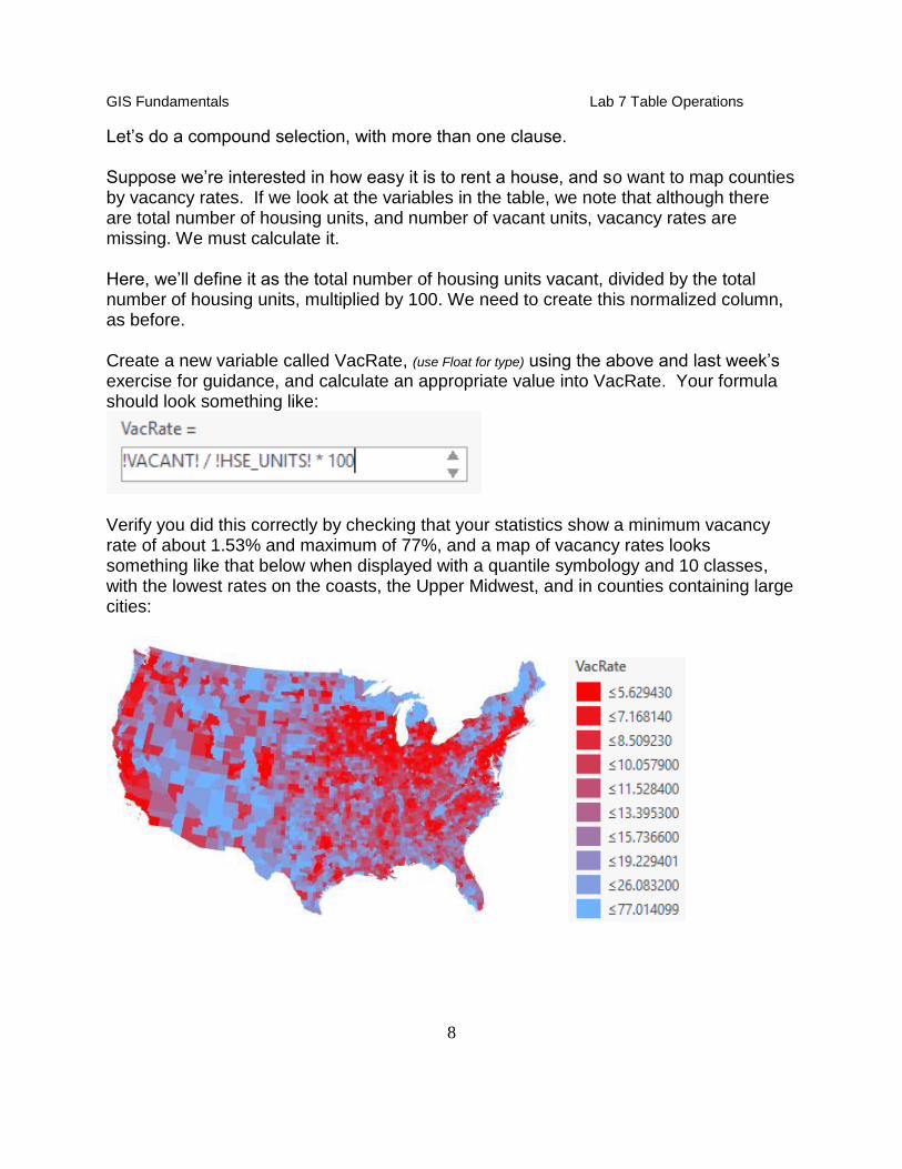
Let’s do a compound selection, with more than one clause. Suppose we’re interested in how easy it is to rent a house, and so want to map counties by vacancy rates. If we look at the variables in the table, we note that although there are total number of housing units, and number of vacant units, vacancy rates are missing. We must calculate it. Here, we’ll define it as the total number of housing units vacant, divided by the total number of housing units, multiplied by 100. We need to create this normalized column, as before. Create a new variable called VacRate, (use Float for type) using the above and last week’s exercise for guidance, and calculate an appropriate value into VacRate. Your formula should look something like:

Verify you did this correctly by checking that your statistics show a minimum vacancy rate of about 1.53% and maximum of 77%, and a map of vacancy rates looks something like that below when displayed with a quantile symbology and 10 classes, with the lowest rates on the coasts, the Upper Midwest, and in counties containing large cities:


9

I want to set an upper threshold of 70% vacancy. I build the clause as above, selecting the target variable (VacRate), the relationship (Is Greater Than), and the threshold (70.0), and then click the ADD button on the right side of the Clause bar. This builds the first clause: I also want to find low vacancy rate counties, so I can Add a Clause by clicking on the button below the current clause: This opens another clause builder window, into which I enter the following:

Here we use the Or operator, because we want to identify vacancy rates that are at the extremes, either high or low.

After I enter the desired parameters and click Add, both clauses show up in the Selection Pane: Clicking on Run applies both of these to the table, selecting records that meet both criteria.


10

Hitting Run should select 6 of 3069 counties, shown in the figure below, and re-colored from previous figures so the selected counties will stand out on the map:

We often want to export results of a query. We’ve already shown you how to export a data layer, both the polygons and table (right click on the layer in the TOC, then Data - Export Features). You may also export just the table through two avenues. First, click on the Menu button in the upper right corner of a displayed table, then select the Export option: The second (not shown), is similar to exporting a layer, right click on the layer in the TOC, then Data – Export Table.


11

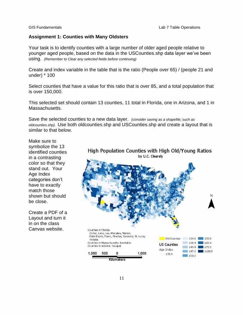
Assignment 1: Counties with Many Oldsters Your task is to identify counties with a large number of older aged people relative to younger aged people, based on the data in the USCounties.shp data layer we’ve been using. (Remember to Clear any selected fields before continuing) Create and index variable in the table that is the ratio (People over 65) / (people 21 and under) * 100 Select counties that have a value for this ratio that is over 85, and a total population that is over 150,000. This selected set should contain 13 counties, 11 total in Florida, one in Arizona, and 1 in Massachusetts. Save the selected counties to a new data layer. (consider saving as a shapefile; such as

oldcounties.shp). Use both oldcounties.shp and USCounties.shp and create a layout that is similar to that below. Make sure to symbolize the 13 identified counties in a contrasting color so that they stand out. Your Age Index categories don’t have to exactly match those shown but should be close. Create a PDF of a Layout and turn it in on the class Canvas website.


12

Joining Two Existing Tables (practice exercise)

We often manage tables separately and join them as needed on common fields for combined analysis. We’ll cover how to join tables in ArcGIS Pro. Create a new project, add a Map, and Add the layer (which is also called a “theme”) demographics.shp from the Lab 7 folder. Also add the data table name more_data.dbf Right click on more_data.dbf in the TOC, and left click on Open Notice that both tables have an item named Blkgrp. This item can serve as a key for the join. As described in the book, the join will match rows by these key variables, to display a combined table. Use the scroll bars at the bottom of each table to look at all the variables (columns) in each table. Are the variables ordinal, nominal, or interval/ratio? Which other variables are found in both tables? Which variables might serve as keys for the table, and which would be inappropriate as keys? See Chapter 8 in the textbook, if you’re unsure on these concepts. Each record (row) in each table corresponds to each polygon in this US Census Bureau demographic data, displayed in demographics. These files were produced from U.S. Census data, which uses a variable named Blkgrp as unique identifiers. The codes correspond to groups of city blocks, and identify polygons used to summarize census data. Each record in our tables corresponds to a block group.


13

The file more_data.dbf includes populations at various dates for each block group polygon, e.g., Hh80=population in 1980, Hh90= population in 1990, etc. Right click on the demographics layer in the TOC select Joins and Relates and then Add Join

(Video: Join Tables)


14

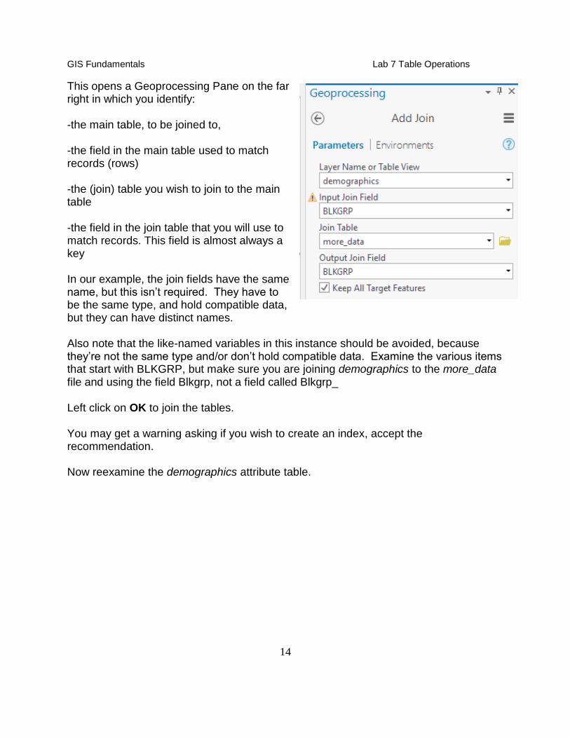
This opens a Geoprocessing Pane on the far right in which you identify: -the main table, to be joined to, -the field in the main table used to match records (rows) -the (join) table you wish to join to the main table -the field in the join table that you will use to match records. This field is almost always a key In our example, the join fields have the same name, but this isn’t required. They have to be the same type, and hold compatible data, but they can have distinct names. Also note that the like-named variables in this instance should be avoided, because they’re not the same type and/or don’t hold compatible data. Examine the various items that start with BLKGRP, but make sure you are joining demographics to the more_data file and using the field Blkgrp, not a field called Blkgrp_ Left click on OK to join the tables. You may get a warning asking if you wish to create an index, accept the recommendation. Now reexamine the demographics attribute table.


15

Notice the demographics table has the more_data fields append to the end of each record.

You’ve just connected the two tables, matching the records in one table to the records in another table that have the same value for BLKGRP. This is a temporary join; the original files/data have not been modified. ArcGIS keeps track of joins within a project, and how to display the various joined files. If you were to display these data sets in another project, they would not appear joined. The data are not copied to a new, combined, file. Rather, this join tells ArcGIS to display these two data sets within this particular view, matching each row by the join variable.

Selecting on a Joined Table Now, let’s select items based on the joined tables.

Open the Attributes Table of demographics. It should display both the original data plus the data from more_data.dbf.

Activate the Select by Attributes described in the previous section of this lab

Specify a selection clause Hhpctgrowt is Greater Than 0 (see right)

Examine your selected block groups on the map, and notice it selects most of them

Clear your selection (from the Main ArcGIS menu, SelectionClear Selected Features), or use the toolbar icon


16

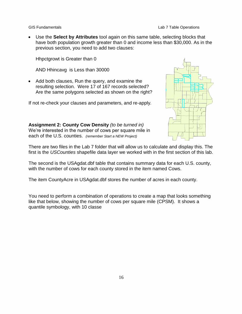
Use the Select by Attributes tool again on this same table, selecting blocks that have both population growth greater than 0 and income less than $30,000. As in the previous section, you need to add two clauses: Hhpctgrowt is Greater than 0 AND Hhincavg is Less than 30000

Add both clauses, Run the query, and examine the resulting selection. Were 17 of 167 records selected? Are the same polygons selected as shown on the right?

If not re-check your clauses and parameters, and re-apply.

Assignment 2: County Cow Density (to be turned in) We’re interested in the number of cows per square mile in each of the U.S. counties. (remember Start a NEW Project)

There are two files in the Lab 7 folder that will allow us to calculate and display this. The first is the USCounties shapefile data layer we worked with in the first section of this lab. The second is the USAgdat.dbf table that contains summary data for each U.S. county, with the number of cows for each county stored in the item named Cows. The item CountyAcre in USAgdat.dbf stores the number of acres in each county. You need to perform a combination of operations to create a map that looks something like that below, showing the number of cows per square mile (CPSM). It shows a quantile symbology, with 10 classe


17

The combined FIPS code in each table may serve as a key to join them. It concatenates the state and county FIPS codes as to uniquely identify each county. (Note: if your map goes blank after the join, use symbology to display unique values; the primary single symbol default display is cleared with the join)

There are 640 acres in a square mile, so you may wish to calculate a variable that holds the number of square miles in each county, and then create another variable into which you calculate the number of cows divided by the number of square miles. Alternately, you can do a combined calculation into a single variable. Create a layout, add a title, legend, your name, scale bar, and North arrow, export a PDF, and turn it in on the course Canvas site.


18

Creating New Tables Creating a table and joining it to existing tables is a common operation. Often, this join involves a one-to-many relationship between tables. Each record in one table matches many records in the second table. For example, a typical county may have approximately 80 different soil types, but over 100,000 different soil polygons of these types. Therefore, we may have properties for each of the 80 different types, e.g., crop productivity, engineering properties, moisture characteristics. We may format these in a table and join this table to our existing county data layer. The repeated properties aren’t copied, just displayed for the appropriate polygon. This saves space, because we don’t have redundant copies of the soil properties information saved for each instance of a soil polygon in our data layer. This exercise will give you practice in creating and joining tables, and the other techniques you learned in the first section of this lab (Video: Create Tables). Create a new Map with a Blank Document. 1. Add the soils.shp data layer, set the Symbology to Unique Values based on the item Soil_Type. 2. Uncheck the “Show all other values”, so this won’t appear in the legend. 3. Select a Color Ramp,.


19

Open the soils attribute table. You should have a view similar to the figure below. Review the layer attributes, and in particular notice the soil_type attribute. The soil_type attribute contains a code corresponding to the soil type of each individual polygon. Notice there are 15 different soil types designated by numbers between 18 and 69. There are 122 different soil polygons.

Our job is to create a new table, enter important information for each of the 15 different soil types, and join this data with the soils data layer. In this exercise you will use the “soil_type” variable in the soils data layer as the join item or join column. This is the “key” variable that will be used to match the rows from the new soil properties table you will create to the soil polygon data in soils. The join item must be defined the same in both tables, with the same type (long or short integer, text, etc.)


20

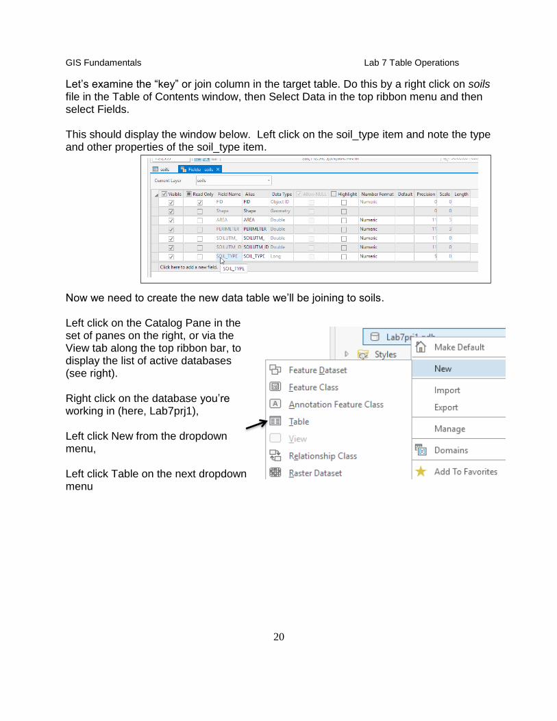
Let’s examine the “key” or join column in the target table. Do this by a right click on soils file in the Table of Contents window, then Select Data in the top ribbon menu and then select Fields. This should display the window below. Left click on the soil_type item and note the type and other properties of the soil_type item.

Now we need to create the new data table we’ll be joining to soils. Left click on the Catalog Pane in the set of panes on the right, or via the View tab along the top ribbon bar, to display the list of active databases (see right). Right click on the database you’re working in (here, Lab7prj1), Left click New from the dropdown menu, Left click Table on the next dropdown menu


21

and complete the form in the Geoprocessing Pane, then Run to create a new table named soilprops. Open the soilprops table (right click in the TOC, then Open). Add the following fields (remember via the table tools icon, Add Field):

soil_type, long

name, text, length of 20

fert_class, double

drain_clas, double.

Do not delete or alter the OID field. If you make a mistake on a field name or type, correct it before you create the next field. After a field is created you cannot edit the field name, you must delete the field and try again. Remember to Save your Fields (at the top ribbon meun) when you are done entering them.

Add the soilprops table to your Map if it isn’t already in your TOC, and Open the

table. You should see the column headings and a blank row. Left click on the table to activate it, then on the soil type cell for the first row. This should put the cell in edit mode, with a green background for the column, and a darkened border around the cell:


22

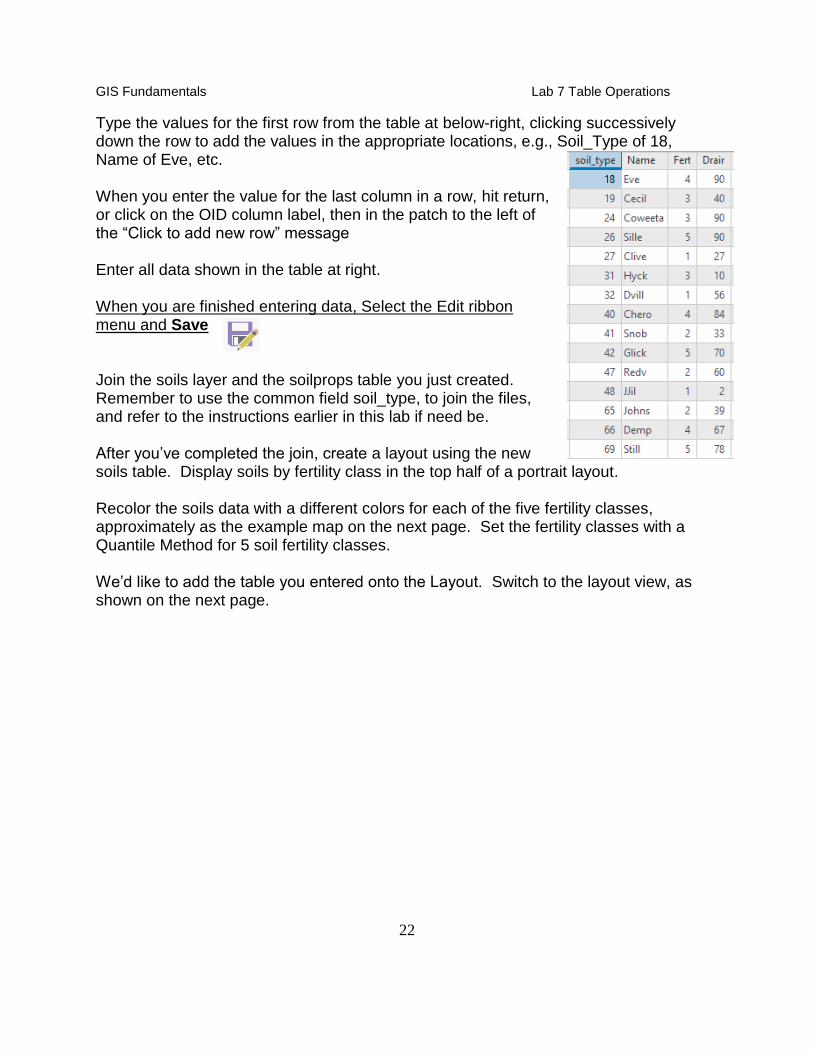
Type the values for the first row from the table at below-right, clicking successively down the row to add the values in the appropriate locations, e.g., Soil_Type of 18, Name of Eve, etc. When you enter the value for the last column in a row, hit return, or click on the OID column label, then in the patch to the left of the “Click to add new row” message Enter all data shown in the table at right. When you are finished entering data, Select the Edit ribbon menu and Save

Join the soils layer and the soilprops table you just created. Remember to use the common field soil_type, to join the files, and refer to the instructions earlier in this lab if need be. After you’ve completed the join, create a layout using the new soils table. Display soils by fertility class in the top half of a portrait layout. Recolor the soils data with a different colors for each of the five fertility classes, approximately as the example map on the next page. Set the fertility classes with a Quantile Method for 5 soil fertility classes. We’d like to add the table you entered onto the Layout. Switch to the layout view, as shown on the next page.


23

Switch to your layout view, Make sure the Insert tab is activated and expand the Map Frame and elements listed in the Contents Pane, by clicking on carets on the left so they point to the lower right, shown in the image at right: Click on the soilprops table in the Contents window, the on the Table Frame tool in the Map Surrounds group, shown near the top center (thick arrow, above center of figure). This will activate a cross-hair cursor, indicating you should draw a Table Frame. Here, click-hold and drag to put one in the lower part of the layout.


24

TO TURN IN as .pdf

Map1: Oldster Counties

Map2: Cow Density

Map3: Macon County, NC Soil Fertility We must stress the utility of what you’ve just done. Managers and scientists often want information grouped and displayed different ways, and joins are then used to add information to and produce maps upon which decisions are based. Geographic data may be joined to many different sets of tabular data. These joined sets may be selected based on many combinations of attributes, greatly increasing the flexibility and utility of data in a GIS.


25

Documents

Lab 7: Tables Operations in ArcGIS - giscourses.cfans.umn.edu · GIS Fundamentals Lab 7 Table Operations 1 Lab 7: Tables Operations in ArcGIS What You’ll Learn: This Lab provides