Embed Size (px)
Citation preview

Lab 2 Analysis of Observational Study/Calculations
with SPSS

What does an article look like? • Title/Title Page • Abstract • Introduction • Method • Results • Discussion • References

What does an article look like? Resources
• See Appendix A in your book for guidance and examples. – WARNING – some things have APA rules have
changed since the book’s publication.
• Purdue Online Writing Lab (OWL) is a good resource for APA styling – http://owl.english.purdue.edu/owl/section/2/10/

RUNNING HEAD: Short Title 1
Title Name(s)
Affiliation
Author Note -------------------------------------------- ---------------------------- -------------------------------------------- -----------------------------------------------
Short Title 2
Abstract
---------------------------------------------------------------------------------------------------------------------------------------------------
Short Title 3
Title
----------------------------------------------------------------------------------------------------
----------------------------------------------- ----------------------------------------------------------------------------------------------------
----------------------------------------------- ----------------------------------------------------------------------------------------------------
-----------------------------------------------
Short Title 4 Method
Subjects ---------------------------------------------------------------------------------------------- Apparatus ---------------------------------------------------------------------------------------------- Procedure ----------------------------------------------------------------------------------------------------------------------------------------------- -------------------------------------------------
Short Title 5 Results
--------------------------------------------------------------------------------------------------------------------------------------------------- ---------------------------------------------------------------------------------------------------------------------------------------------------------------------------------------------------------------------------------------------------------------------------------------------------------------------------------------------------------
Short Title 6 Discussion
--------------------------------------------------------------------------------------------------------------------------------------------------- ---------------------------------------------------------------------------------------------------------------------------------------------------------------------------------------------------------------------------------------------------------------------------------------------------------------------------------------------------------
Short Title 8 References
----------------------------------------------------------------------------------------------
----------------------------------------------------------------------------------------------
----------------------------------------------------------------------------------------------
----------------------------------------------------------------------------------------------
----------------------------------------------------------------------------------------------------
---------------------------------------
Short Title 9 Footnotes
1.--------------------------------------------------------------------------------------------------------------------------------------------------- 2.---------------------------------------------------------------------------------------------------------------------------------------------------
Short Title 10 Table 1 Title of Table ___________________ ___________________ ----- ---- ---- --- ----- ---- ---- --- _________________
Short Title 11 (put figures here with one figure per page) Figure1.---------------------------------------------------------------------------------------------------------------------------------------------------

General Formating Tidbits • Margins are 1 inch left, right, top, bottom • Font is 12 point Times New Roman • Double Space EVERYTHING • Round numbers to two decimal places • Page numbers go at the top right except on
Figure pages

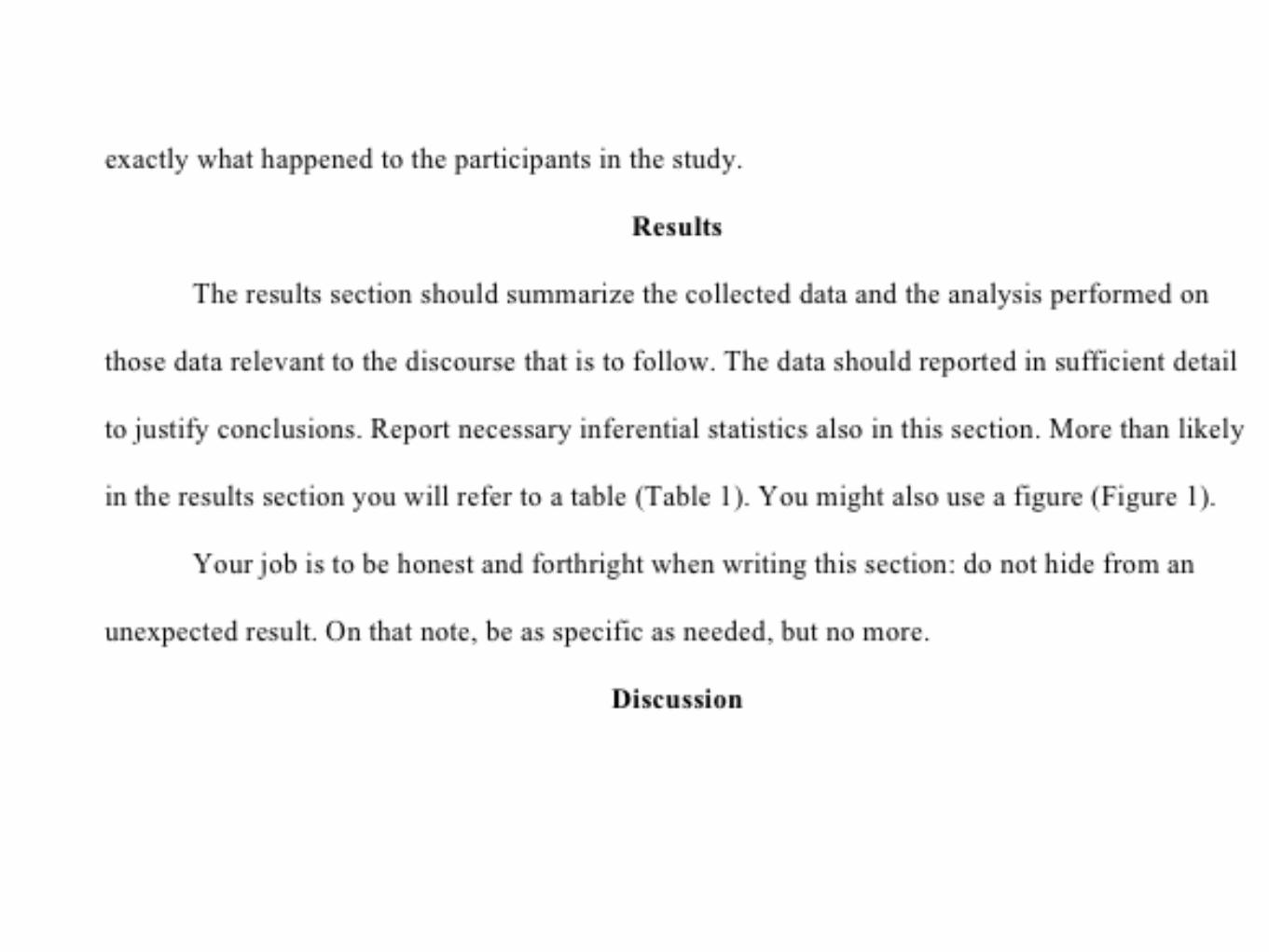
Results • Direct the reader to data that seem most relevant to the
purpose of the research. • Structure 1. State the purpose of the analysis. 2. Identify the descriptive statistic to be used to summarize the
results. May report interrater reliability here. 3. Present a summary of this descriptive statistic across conditions
in the text itself, in a table, or in a figure. – If you use a table or figure point out the major finding the
reader should focus on. 4. Present the inferential statistics that are relevant for evaluating
the descriptive statistics. 5. State the conclusion that follows from each test, but do not
discuss implications. No causal statements!

Schachter et al. (1991) • The results of these observations are in Table 1, which
presents the mean uhs per minute of speaking for these 10 departments. Ignoring momentarily the a priori assignment of departments to the humanities or sciences, let us ask first if these 10 departments differ from one another in their lecturers' tendency to use uhs and ahs. They do, F(9,35) = 2.87, p < .01. It is also evident that, with the exception of philosophy, these differences correspond to the sciences-versus-humanities distinction, for the natural sciences average 1.39 uhs per minute in their lectures; the social sciences, 3.84; and the humanities, 4.85, F(2,42) = 6.46, p < .01. The natural sciences differ, using protected t tests, from the social sciences ( p < .02) and from the humanities (p < .01), whereas the social sciences and the humanities do not differ significantly from one another.
Do the departments differ from
each other?
Do the disciplines differ from
each other?

What if there were just 2 lectures? • Imagine if Schachter et al. (1991) had only
compared 2 lectures (Biology vs Art History). Then their write up might have looked a lot different.
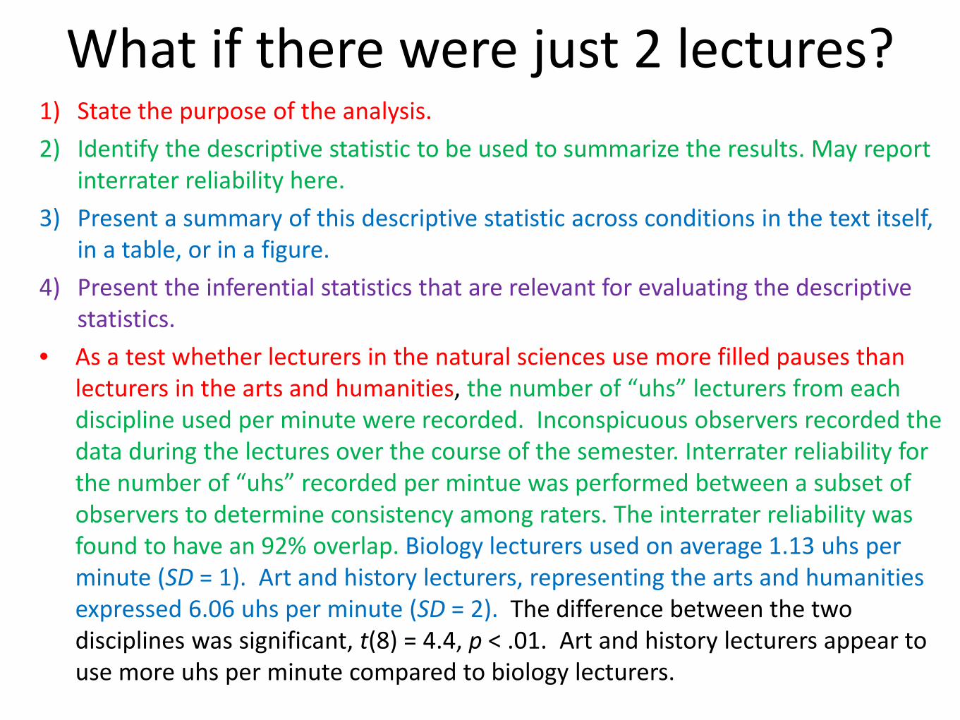
• As a test whether lecturers in the natural sciences use more filled pauses than lecturers in the arts and humanities, the number of “uhs” lecturers from each discipline used per minute were recorded. Inconspicuous observers recorded the data during the lectures over the course of the semester. Interrater reliability for the number of “uhs” recorded per mintue was performed between a subset of observers to determine consistency among raters. The interrater reliability was found to have an 92% overlap. Biology lecturers used on average 1.13 uhs per minute (SD = 1). Art and history lecturers, representing the arts and humanities expressed 6.06 uhs per minute (SD = 2). The difference between the two disciplines was significant, t(8) = 4.4, p < .01. Art and history lecturers appear to use more uhs per minute compared to biology lecturers.

What if there were just 2 lectures? 1) State the purpose of the analysis. • As a test whether lecturers in the natural sciences use more filled
pauses than lecturers in the arts and humanities, the number of “uhs” lecturers from each discipline used per minute were recorded. Inconspicuous observers recorded the data during the lectures over the course of the semester. Interrater reliability for the number of “uhs” recorded per mintue was performed between a subset of observers to determine consistency among raters. The interrater reliability was found to have an 92% overlap. A subset of Biology lecturers used on average 1.13 uhs per minute (SD = 1). Art and history lecturers, representing the arts and humanities expressed 6.06 uhs per minute (SD = 2). The difference between the two disciplines was significant, t(8) = 4.4, p < .01. Art and history lecturers appear to use more uhs per minute compared to biology lecturers.

What if there were just 2 lectures? 1) State the purpose of the analysis. 2) Identify the descriptive statistic to be used to summarize the results.
May report interrater reliability here. • As a test whether lecturers in the natural sciences use more filled
pauses than lecturers in the arts and humanities, the number of “uhs” lecturers from each discipline used per minute were recorded. Inconspicuous observers recorded the data during the lectures over the course of the semester. Interrater reliability for the number of “uhs” recorded per mintue was performed between a subset of observers to determine consistency among raters. The interrater reliability was found to have an 92% overlap. Biology lecturers used on average 1.13 uhs per minute (SD = 1). Art and history lecturers, representing the arts and humanities expressed 6.06 uhs per minute (SD = 2). The difference between the two disciplines was significant, t(8) = 4.4, p < .01. Art and history lecturers appear to use more uhs per minute compared to biology lecturers.

What if there were just 2 lectures? 1) State the purpose of the analysis. 2) Identify the descriptive statistic to be used to summarize the results. May report
interrater reliability here. 3) Present a summary of this descriptive statistic across conditions in the text itself,
in a table, or in a figure. • As a test whether lecturers in the natural sciences use more filled pauses than
lecturers in the arts and humanities, the number of “uhs” lecturers from each discipline used per minute were recorded. Inconspicuous observers recorded the data during the lectures over the course of the semester. Interrater reliability for the number of “uhs” recorded per mintue was performed between a subset of observers to determine consistency among raters. The interrater reliability was found to have an 92% overlap. Biology lecturers used on average 1.13 uhs per minute (SD = 1). Art and history lecturers, representing the arts and humanities expressed 6.06 uhs per minute (SD = 2). The difference between the two disciplines was significant, t(8) = 4.4, p < .01. Art and history lecturers appear to use more uhs per minute compared to biology lecturers.
What if there were just 2 lectures? 1) State the purpose of the analysis. 2) Identify the descriptive statistic to be used to summarize the results. May report
interrater reliability here. 3) Present a summary of this descriptive statistic across conditions in the text itself,
in a table, or in a figure. 4) Present the inferential statistics that are relevant for evaluating the descriptive
statistics. • As a test whether lecturers in the natural sciences use more filled pauses than
lecturers in the arts and humanities, the number of “uhs” lecturers from each discipline used per minute were recorded. Inconspicuous observers recorded the data during the lectures over the course of the semester. Interrater reliability for the number of “uhs” recorded per mintue was performed between a subset of observers to determine consistency among raters. The interrater reliability was found to have an 92% overlap. Biology lecturers used on average 1.13 uhs per minute (SD = 1). Art and history lecturers, representing the arts and humanities expressed 6.06 uhs per minute (SD = 2). The difference between the two disciplines was significant, t(8) = 4.4, p < .01. Art and history lecturers appear to use more uhs per minute compared to biology lecturers.

What if there were just 2 lectures? 1) State the purpose of the analysis. 2) Identify the descriptive statistic to be used to summarize the results. May report interrater
reliability here. 3) Present a summary of this descriptive statistic across conditions in the text itself, in a table, or
in a figure. 4) Present the inferential statistics that are relevant for evaluating the descriptive statistics. 5) State the conclusion that follows from each test, but do not discuss implications. No causal
statements!
• As a test whether lecturers in the natural sciences use more filled pauses than lecturers in the arts and humanities, the number of “uhs” lecturers from each discipline used per minute were recorded. Inconspicuous observers recorded the data during the lectures over the course of the semester. Interrater reliability for the number of “uhs” recorded per mintue was performed between a subset of observers to determine consistency among raters. The interrater reliability was found to have an 92% overlap. Biology lecturers used on average 1.13 uhs per minute (SD = 1). Art and history lecturers, representing the arts and humanities expressed 6.06 uhs per minute (SD = 2). The difference between the two disciplines was significant, t(8) = 4.4, p < .01. Art and history lecturers appear to use more uhs per minute compared to biology lecturers.
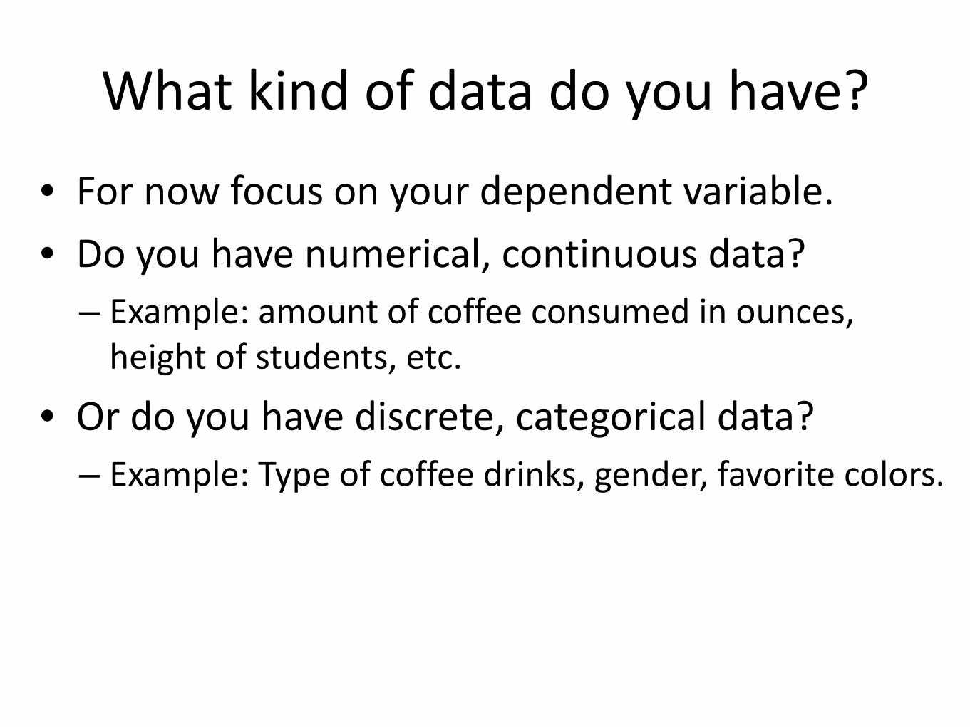
What kind of data do you have?
• For now focus on your dependent variable. • Do you have numerical, continuous data?
– Example: amount of coffee consumed in ounces, height of students, etc.
• Or do you have discrete, categorical data? – Example: Type of coffee drinks, gender, favorite colors.

If you have continuous data...
• We generally summarize the data with means and standard deviations.
• As long as we can reasonably assume that – One observation is independent from another
observation. – You can reasonably assume the sampling distribution
of the mean is normal.

How to generate descriptive statistics once data is entered into
SPSS. • Analysis Descriptive Statistics Explore

The Explore Window • When you choose Analyze >>
Descriptives >> Explore this window will appear.
• Drop the variable you want descriptives on into the Dependent List (e.g., DrinkSize, which is the Dependent Variable (DV)).
• If you have an Independent Variable (IV) that has a small number of levels (e.g., TimeOfDay) then drop that variable into the Factor List.
• Click OK.
• SPSS will calculate descriptive statistics conditional on each level of the IV factor.

An output window will appear
Morning M = 8.40 SD = 3.28
Afternoon M = 16.80 SD = 5.02

If you want to run a t-test... Analyze Compare Means Independent-Samples T Test

Independent Sample t-Test Window
Drop your DV (e.g., DrinkSize) into Test Variables
Drop you IV (e.g., TimeOfDay) in Grouping Variables
Don’t forget to “Define Groups...”

Define Groups
Once you are in “Define Groups” (directly below)You must tell SPSS what the values of the grouping variable (IV) are.
With the grouping variable highlighted, press “Define Groups”
Enter the values for the IV
After you have it set up -Click “Continue” -Click “OK”

The output looks like this
The important parts!

Basic Reporting of Results
• When you describe your data with means and standard deviations and make inferences with t-tests use a sentence like this to describe your data: – Larger drinks were observed in the afternoon
hours (M = 16.80, SD = 5.02) than in the morning hours (M = 8.40, SD = 3.28; t(8) = -3.13, p < .05). • Notice M, SD, t, and p are all italicized.

If you have categorical data...
• We summarize the data in proportions or sometimes frequencies.
• Again we assume independence between observations.
• Also generally require large sample sizes, at least 5 observations per cell or condition.

Chi-Square Test
• Can we conclude that people in different parties have different attitudes? • Conceptually we are interested whether knowing something about the
political party tells us something about people’s attitudes. • The Chi-Square test examines if there is a relationship between political
party and the attitude one has.
Attitude Against For Total
Party
Democrat 8 2 10
Republican 3 7 10
Total 11 9 20

How to generate descriptive statistics once data are entered in SPSS.
If you hit this “1<-> A” button you can go back and fourth between the assigned numbers and the “Value Names” you can assign by clicking on the “Variable View” at the bottom of the SPSS window. This is also where you name your columns at.

How to generate descriptive statistics once data are entered in SPSS.
Analyze Descriptive Statistics Crosstabs
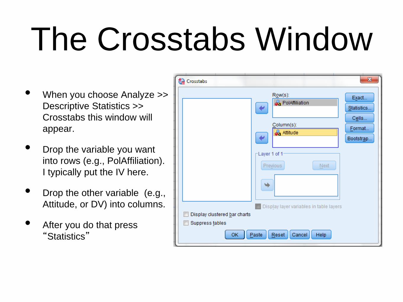
The Crosstabs Window • When you choose Analyze >>
Descriptive Statistics >> Crosstabs this window will appear.
• Drop the variable you want into rows (e.g., PolAffiliation). I typically put the IV here.
• Drop the other variable (e.g., Attitude, or DV) into columns.
• After you do that press “Statistics”
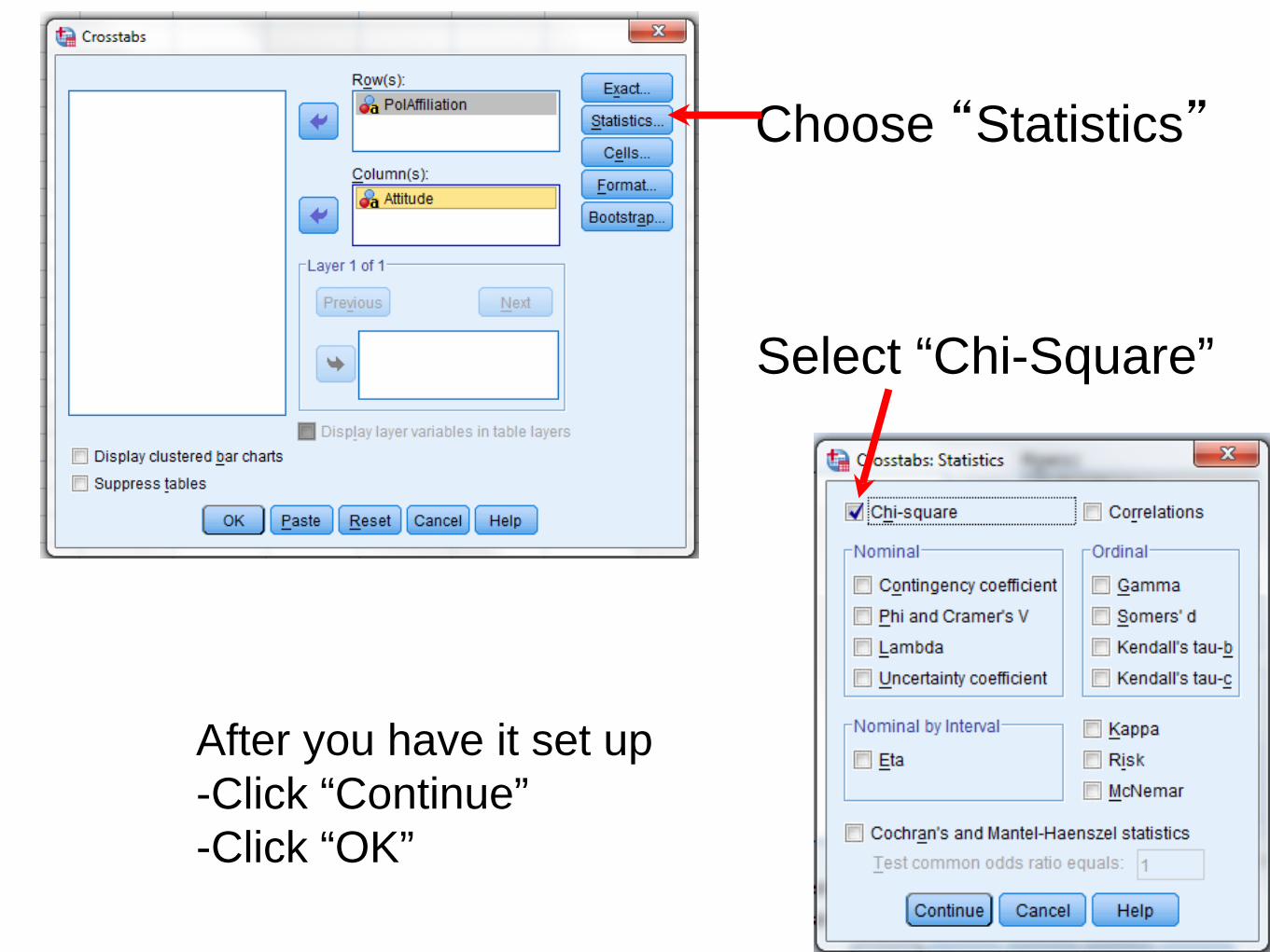
Choose “Statistics”
Select “Chi-Square”
After you have it set up -Click “Continue” -Click “OK”

An output window will appear
This table will tell you about the distribution of observations. For example, 8 Democrats out of 10
were against.
This table will tell you about the outcome of the Pearson Chi-Square test of independence. Use
the top line – “Pearson Chi-Square”

Writing up the results
• When you describe your data with proportions and make inferences with Chi-Square tests, we use a sentence like this to describe the data:
• Seventy percent of republicans reported strong attitudes for the bill as compared to only 20% of Democrats, χ2(1, N = 20) = 5.1, p < .05.
Degrees of freedom Note in APA style when you start a sentence with a number you spell it out.

Now, crunch that data!