1

Georgia Institute of TechnologySchool of Earth and Atmospheric Sciences

EAS 4641Spring 2007

Lab 2Introduction to Quantitative Analysis: Chemistry

Purpose of Lab 2:1) To learn some basic analytical chemistry definitions and techniques2) Understand the general function of analytical instruments and how to calibrate

(We will calibrate an IC, this calibration will be used for a later experiment andmeasurements of ambient air chemical components).

3) To begin to consider measurement uncertainties and intro. to linear regression.

Volumetric GlasswareVolumetric laboratory glassware includes volumetric flasks, pipettes, and burettes.Beakers, graduated cylinders, Erlenmeyer flasks, and test tubes are not volumetricglassware. Volumetric glassware is calibrated by the manufacturer to deliver (TD) orcontain (TC) a known exact volume of liquid at standard conditions: 20 degrees Celsiusand 1 atmosphere pressure. Volumetric glassware will have identification of the volumeand the volume tolerance etched onto the glass. Often, ambient laboratory conditions arenot identical to standard conditions, therefore the volumes dispensed or contained involumetric glassware are often not the same as the manufacturer's specifications, butwithin some acceptable limits (± % tolerance) determined by the manufacturer. Thisslight variation in volume will cause a systematic error when making solutions that arebased on volume-volume or mass-volume concentrations.

"Chapter 2: Tools of the Trade," from Quantitative Chemical Analysis 4th Ed. By D.C. Harris, 1995.

Serial DilutionsA serial dilution is a set of solutions with exact concentrations created from astandardized primary solution of a known concentration.

For example, a student will need to create 5 solutions (5E-5, 1E-5, 5E-6, 1E-6, and 5E-7M NaNO3) from a primary standard of 5x10-3 M NaNO3 in order to complete anassignment. To do so, serial dilutions will be required from the primary standard, 5x10-3

M NaNO3 (Note: the 5x10-3 M NaNO3 standard will be made from a 0.5 M NaNO3

solution). One viable method could be:

5 x 10-5 M = 1 ml of 5x10-3 M NaNO3 into 100-ml volumetric flask, fill to themark, shake well.

2

1 x 10-5 M = 200 µl of 5 x 10-3 M NaNO3 into 100-ml volumetric flask, fill tothe mark, shake well.

…and so on.

The mathematics involved when deciding how to construct your serial dilutionfollows the volumetric law:

Where C1 is the concentration of the stock solution, V1 the volume of the stocksolution to be diluted into the volume V2, to give the concentration C2. In thiscase,

For the NaNO3 dilution from 1 M to 0.1 M solution, the relationship will be

Analytical MeasurementsAnalytical instruments (IC, spectrophotometer, chemiluminescence, pH meter, GC, massspec, etc) process chemical and physical information in similar ways.

Measurement Limitations (Uncertainty Analysis)Measurements of chemical data have limitations. These limitations are either inherent tothe analytical equipment performing the measurement or to the operator using theequipment. The precision describes the reproducibility of the data. It is a measure ofhow carefully the result is determined without reference to any true value (precision isrelated to uncertainty, e.g., Dx) Three terms are used to describe the precision of a set ofreplicate data: standard deviation, variance, and coefficient of variation.Accuracy describes the correctness of an experimental data, or how close themeasurement is to the exact value. Accuracy is expressed in terms of either absoluteerror or relative error. The error is the difference between an average measurement and

Input ‡ Transform ‡ Detection ‡ SignalFactor Level: Concentration or other quantity to be determined (x-axis)Input: Chemical data (factor) digital or analog signal. (transducer).Transform: Computation, operation, amplification or alteration of the digital or analogsignal.Detection: Processing or conversion of the amplified or altered digital or analog signalto a number.Signal: Output of instrument. Response (y-axis)

ml

mlMM

100

1011.0

¥=

3

an accepted value of the species measured. There are two kinds of errors: random andsystematic errors. Whenever analytical measurements are repeated on the same sample,the data obtained are scattered because of the presence of random errors. These errorsreflect on the precision of the data. Systematic errors have a definite value, an assignablecause, and are of the same sign and magnitude for replicate measurements made inexactly the same way. Systematic errors lead to bias in a technique. Systematic errorshave three sources:

• Instrumental errors (e.g., drift in electronic circuit, leakage in vacuum systems,temperature effects on detectors, current spikes, and calibration errors in meters,weights, and volumetric equipment). To detect and correct instrumental errors,calibrations with suitable standards have to be performed periodically.

• Personal errors (e.g., judgment, prejudice). To minimize personal errors, mostscientists develop the habit of systematically double-checking instrumentreadings, notebook entries, and calculations, or use automated systems to measuredata.

• Method errors (e.g., non-ideal chemical and physical behavior of reagents andreactions: incompleteness of reactions, losses by volatility, adsorption problems,etc.). To minimize method errors, the methods have to be validated with standardmaterials that resemble the samples to be analyzed both in physical state and inchemical composition.

Reporting Accuracy of MeasurementsUse an associated uncertainty to indicate the accuracy of the measurementß Absolute uncertainty is Dx, i.e., Response = 590. ± 18 a.u.ß Relative uncertainty, is Dx/x, i.e.,. Response = 590 a.u. ± 3% (also

referred to as the precision, i.e., Dx of 1 inch in 1 mile is a precisemeasurement, Dx of 1 inch in 5 inches is an imprecise measurement.

When reporting measurement uncertainties, typically one significant fig. is best, 2sig figs in cases of high precision.(unless the first digit is a 1 or 2, i.e., don’t write ± 0.1do write ± 0.12)

The reported value (i.e., x in x ± Dx) last sig fig should be of similar order ofmagnitude as the uncertainty, i.e., 56.01±3 should be 56±3, the uncertainty determineshow you write the best estimate value.

Calibration Curves: How to measure a quantity of interest.

Analytical equipment is usually optimized to detect and report chemical information ofone specific factor (chemical reaction, concentration, analyte, or component of the systemunder investigation) within a specific range of parameters and factor levels. However,not all levels of the factor can be detected. In order to accurately describe the instrumentresponse to factor level intensity, it is necessary to test the response against a series ofknown standards. This is called calibrating the instrument. The result will be a plot ofresponse vs. factor intensity, known as the calibration curve.

4

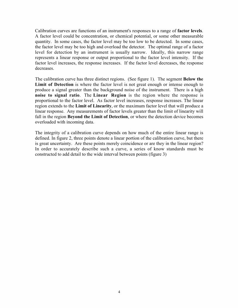
Calibration curves are functions of an instrument's responses to a range of factor levels.A factor level could be concentration, or chemical potential, or some other measurablequantity. In some cases, the factor level may be too low to be detected. In some cases,the factor level may be too high and overload the detector. The optimal range of a factorlevel for detection by an instrument is usually narrow. Ideally, this narrow rangerepresents a linear response or output proportional to the factor level intensity. If thefactor level increases, the response increases. If the factor level decreases, the responsedecreases.

The calibration curve has three distinct regions. (See figure 1). The segment Below theLimit of Detection is where the factor level is not great enough or intense enough toproduce a signal greater than the background noise of the instrument. There is a highnoise to signal ratio. The Linear Region is the region where the response isproportional to the factor level. As factor level increases, response increases. The linearregion extends to the Limit of Linearity, or the maximum factor level that will produce alinear response. Any measurements of factor levels greater than the limit of linearity willfall in the region Beyond the Limit of Detection, or where the detection device becomesoverloaded with incoming data.

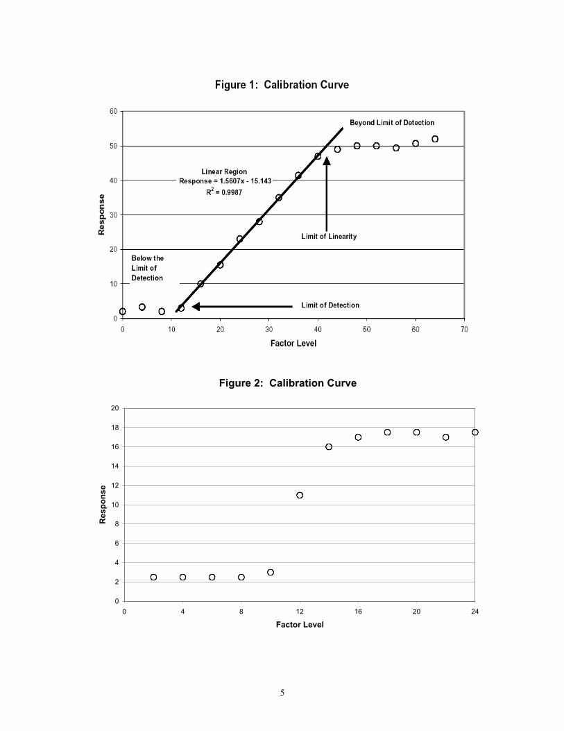
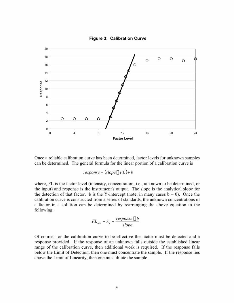
The integrity of a calibration curve depends on how much of the entire linear range isdefined. In figure 2, three points denote a linear portion of the calibration curve, but thereis great uncertainty. Are these points merely coincidence or are they in the linear region?In order to accurately describe such a curve, a series of know standards must beconstructed to add detail to the wide interval between points (figure 3)

5

Figure 2: Calibration Curve

0

2

4

6

8

10

12

14

16

18

20

0 4 8 12 16 20 24

Factor Level

Res

po

nse

6

Once a reliable calibration curve has been determined, factor levels for unknown samplescan be determined. The general formula for the linear portion of a calibration curve is

where, FL is the factor level (intensity, concentration, i.e., unknown to be determined, orthe input) and response is the instrument's output. The slope is the analytical slope forthe detection of that factor. b is the Y-intercept (note, in many cases b = 0). Once thecalibration curve is constructed from a series of standards, the unknown concentrations ofa factor in a solution can be determined by rearranging the above equation to thefollowing.

Of course, for the calibration curve to be effective the factor must be detected and aresponse provided. If the response of an unknown falls outside the established linearrange of the calibration curve, then additional work is required. If the response fallsbelow the Limit of Detection, then one must concentrate the sample. If the response liesabove the Limit of Linearity, then one must dilute the sample.

( ) bFLsloperesponse +¥=

slope

bresponsexFL junk

-==

Figure 3: Calibration Curve

0

2

4

6

8

10

12

14

16

18

20

0 4 8 12 16 20 24

Factor Level

Res

po

nse

7

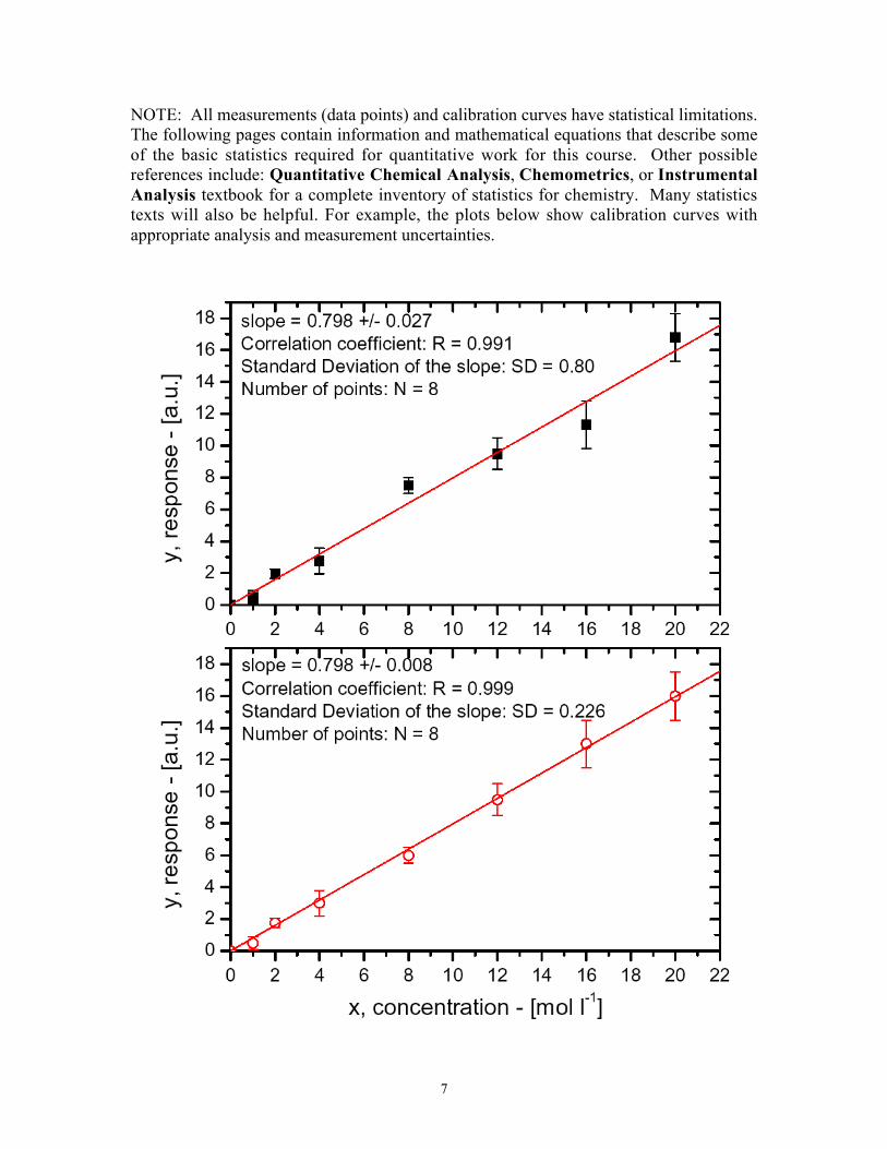
NOTE: All measurements (data points) and calibration curves have statistical limitations.The following pages contain information and mathematical equations that describe someof the basic statistics required for quantitative work for this course. Other possiblereferences include: Quantitative Chemical Analysis, Chemometrics, or InstrumentalAnalysis textbook for a complete inventory of statistics for chemistry. Many statisticstexts will also be helpful. For example, the plots below show calibration curves withappropriate analysis and measurement uncertainties.

8

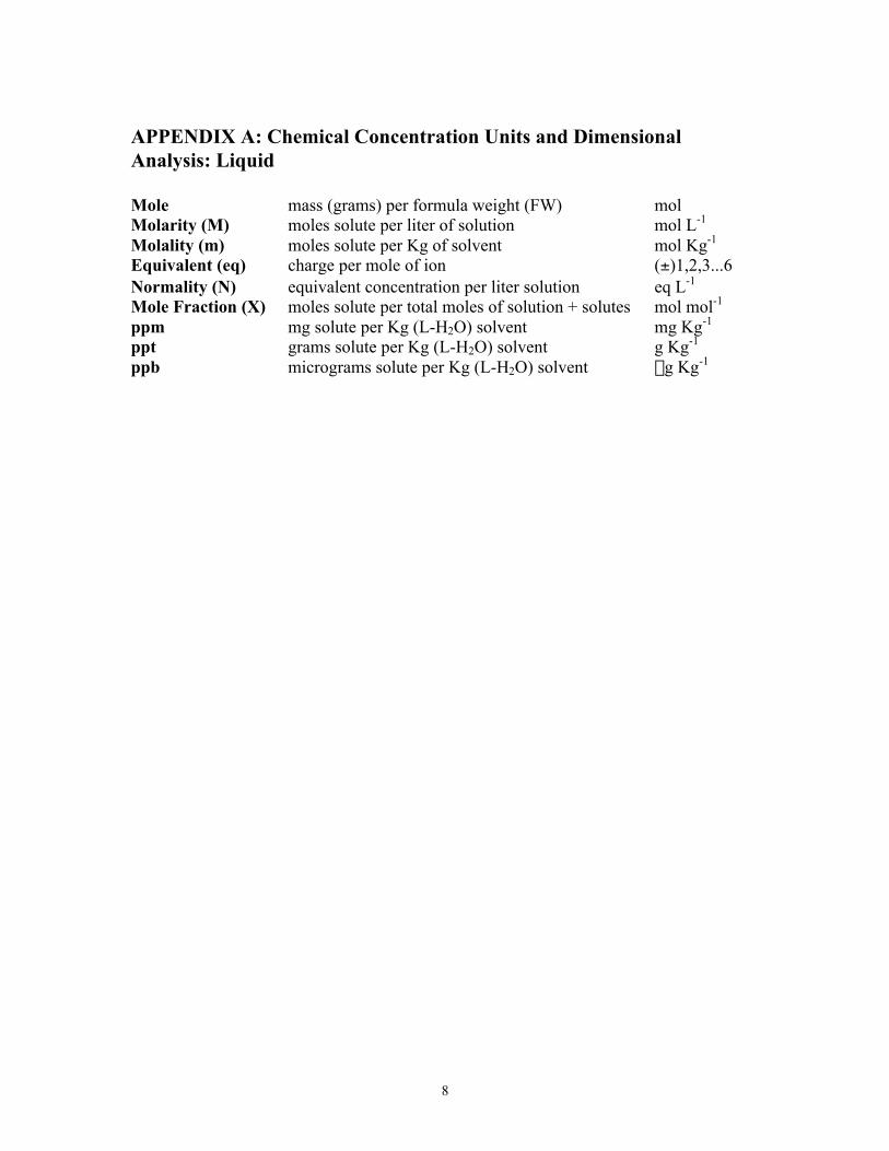
APPENDIX A: Chemical Concentration Units and DimensionalAnalysis: Liquid

Mole mass (grams) per formula weight (FW) molMolarity (M) moles solute per liter of solution mol L-1

Molality (m) moles solute per Kg of solvent mol Kg-1

Equivalent (eq) charge per mole of ion (±)1,2,3...6Normality (N) equivalent concentration per liter solution eq L-1

Mole Fraction (X) moles solute per total moles of solution + solutes mol mol-1

ppm mg solute per Kg (L-H2O) solvent mg Kg-1

ppt grams solute per Kg (L-H2O) solvent g Kg-1

ppb micrograms solute per Kg (L-H2O) solvent mg Kg-1

9

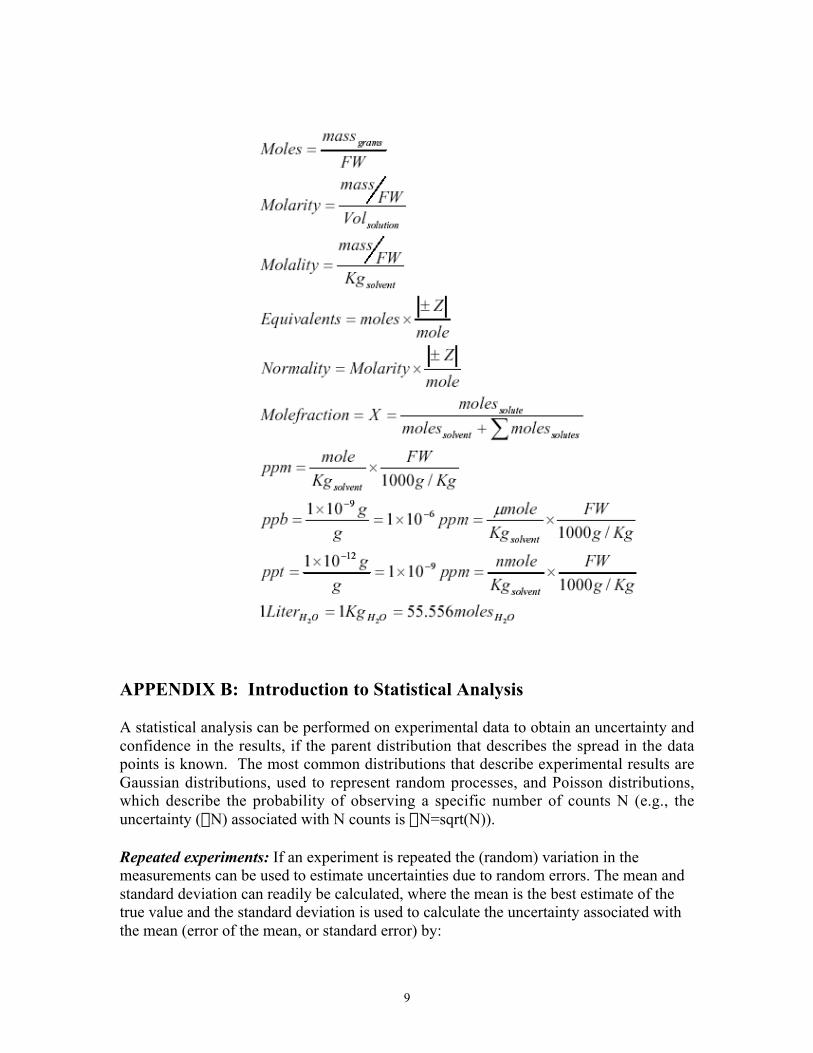
APPENDIX B: Introduction to Statistical Analysis

A statistical analysis can be performed on experimental data to obtain an uncertainty andconfidence in the results, if the parent distribution that describes the spread in the datapoints is known. The most common distributions that describe experimental results areGaussian distributions, used to represent random processes, and Poisson distributions,which describe the probability of observing a specific number of counts N (e.g., theuncertainty (DN) associated with N counts is DN=sqrt(N)).

Repeated experiments: If an experiment is repeated the (random) variation in themeasurements can be used to estimate uncertainties due to random errors. The mean andstandard deviation can readily be calculated, where the mean is the best estimate of thetrue value and the standard deviation is used to calculate the uncertainty associated withthe mean (error of the mean, or standard error) by:

10

error of the mean = std/sqrt(N)

For similar experiments, the uncertainty associated with each measurement is similar andequal to approximately 1 standard deviation. Repeating the experiment reduces theuncertainty of the mean, however, standard error is weak function of N so the benefitrapidly decreases as N gets large (max. of 10 is best). In summary,

Mean ± standard error multiple measurementsX ± stdev one measurement

Confidence intervals: Confidence intervals are another way to specify the uncertainty ofa measurement. The confidence interval is the range over which the true value isexpected, with a given degree of confidence. Confidence intervals can be readilycalculated with current software for linear regression results, (e.g., slopes and intercepts).

1-s = 68.3% confidence interval: eg: x ± Dx, where Dx = s = stdev: this meansthat you are 68% confident that x is within x-Dx and x+Dx, if random errors are normallydistributed. Or there is a 68% probability the true value will be within ±1 s of eitherside of the measurement. (The area under the normal curve bounded by ±1 stdev fromthe mean is 0.68)

2-s = 95.4% confidence intervals:3-s = 99.7% confidence intervals:

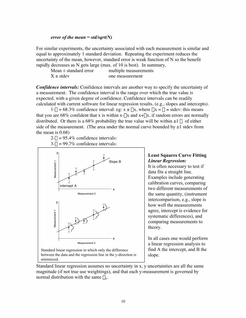
Least Squares Curve FittingLinear Regression:It is often necessary to test ifdata fits a straight line.Examples include generatingcalibration curves, comparingtwo different measurements ofthe same quantity, (instrumentintercomparison, e.g., slope ishow well the measurementsagree, intercept is evidence forsystematic differences), andcomparing measurements totheory.

In all cases one would performa linear regression analysis tofind A the intercept, and B theslope.

Standard linear regression assumes no uncertainty in x, y uncertainties are all the samemagnitude (if not true use weightings), and that each y-measurement is governed bynormal distribution with the same sy.

Mea

sure

men

t 1

Measurement 2

intercept A

Slope B

Mea

sure

men

t 1

Measurement 2

x

x

y

y

Standard linear regression in which only the differencebetween the data and the regression line in the y-direction isminimized.

11

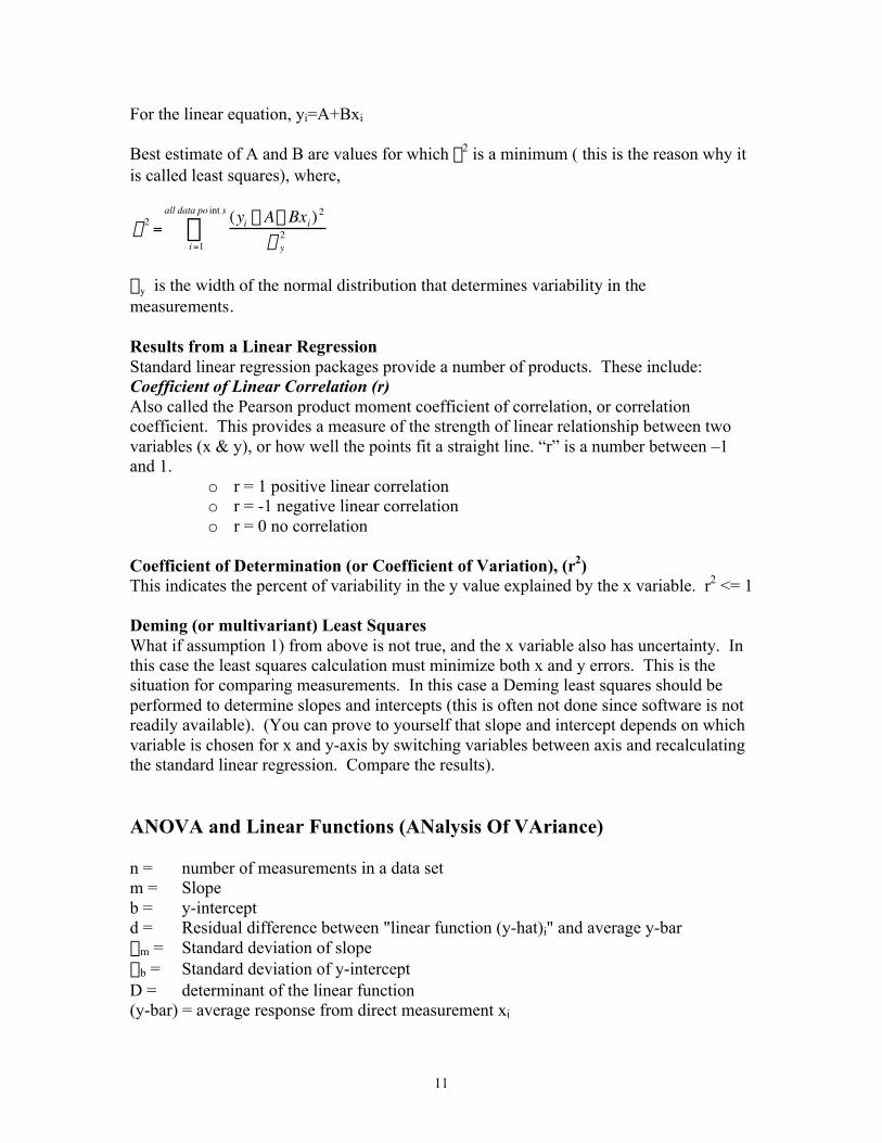
For the linear equation, yi=A+Bxi

Best estimate of A and B are values for which c2 is a minimum ( this is the reason why itis called least squares), where,

c 2 =(yi - A- Bxi)2

s y2

i =1

all data po int s

Â

sy is the width of the normal distribution that determines variability in themeasurements.

Results from a Linear RegressionStandard linear regression packages provide a number of products. These include:Coefficient of Linear Correlation (r)Also called the Pearson product moment coefficient of correlation, or correlationcoefficient. This provides a measure of the strength of linear relationship between twovariables (x & y), or how well the points fit a straight line. “r” is a number between –1and 1.

o r = 1 positive linear correlationo r = -1 negative linear correlationo r = 0 no correlation

Coefficient of Determination (or Coefficient of Variation), (r2)This indicates the percent of variability in the y value explained by the x variable. r2 <= 1

Deming (or multivariant) Least SquaresWhat if assumption 1) from above is not true, and the x variable also has uncertainty. Inthis case the least squares calculation must minimize both x and y errors. This is thesituation for comparing measurements. In this case a Deming least squares should beperformed to determine slopes and intercepts (this is often not done since software is notreadily available). (You can prove to yourself that slope and intercept depends on whichvariable is chosen for x and y-axis by switching variables between axis and recalculatingthe standard linear regression. Compare the results).

ANOVA and Linear Functions (ANalysis Of VAriance)

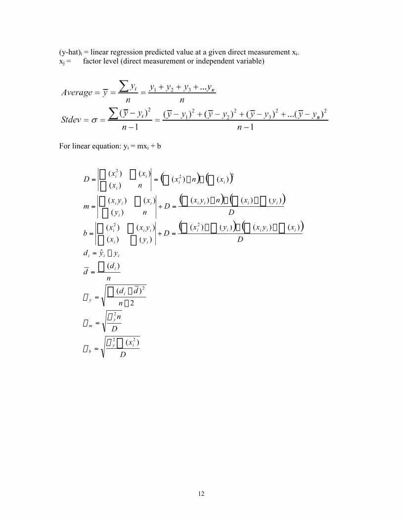
n = number of measurements in a data setm = Slopeb = y-interceptd = Residual difference between "linear function (y-hat)i" and average y-barsm = Standard deviation of slopesb = Standard deviation of y-interceptD = determinant of the linear function(y-bar) = average response from direct measurement xi

12

(y-hat)i = linear regression predicted value at a given direct measurement xi.xj = factor level (direct measurement or independent variable)

For linear equation: yi = mxi + b

( ) ( )

( ) ( )

( ) ( )

( )˙˙˚

˘

ÍÍÎ

È

¥

¥--+

¥

-¥+¥=

-=

=

=

-

-=

=

-=

¥-¥=÷=

¥-¥=÷=

-¥==

+=

ÂÂ

Â

Â

Â

ÂÂÂÂÂÂ

ÂÂ

ÂÂÂÂ

ÂÂ

ÂÂÂÂÂ

mD

xby

D

x

mD

byn

me

m

byx

D

x

D

n

n

dd

n

dd

yyd

D

xyxyxD

yx

yxxb

D

yxnyxD

ny

xyxm

xnxnx

xxD

bmxy

ijijyx

jj

iyb

ym

iy

i

iii

iiiii

ii

iii

iiii

i

iii

iii

ii

i

j

)()(2

)(1

)(

2

)(

)(

ˆ

)()()()(

)()(

)()(

)()()(

)(

)()(

)()()(

)()(

2

2

2

2

2

22

2

2

22

222

s

ss

ss

s

13

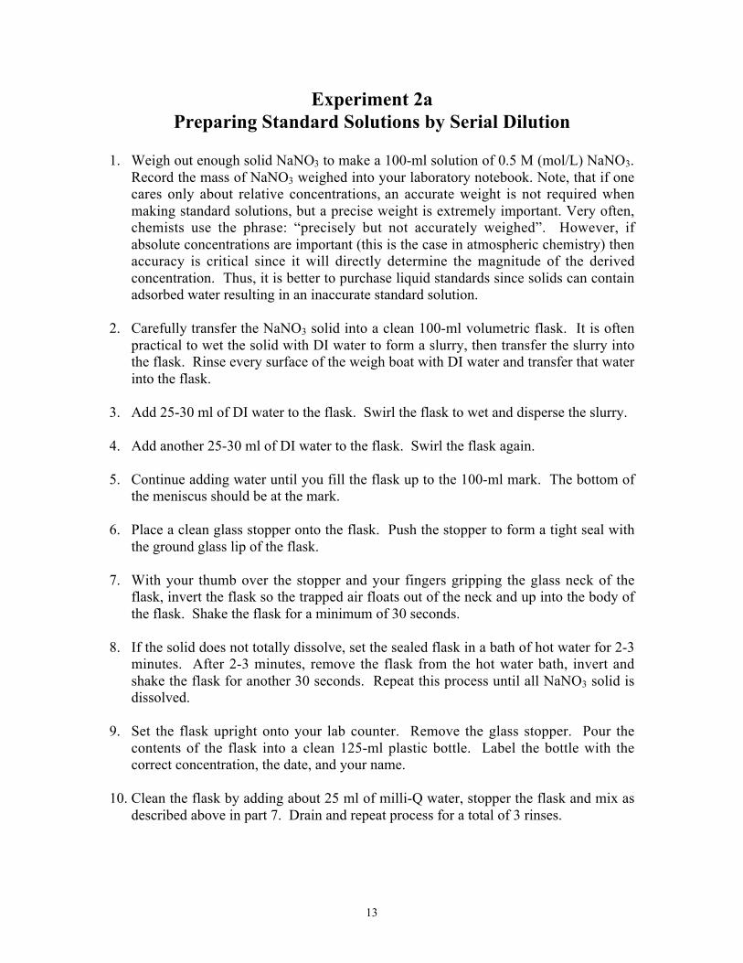
Experiment 2aPreparing Standard Solutions by Serial Dilution

1. Weigh out enough solid NaNO3 to make a 100-ml solution of 0.5 M (mol/L) NaNO3.Record the mass of NaNO3 weighed into your laboratory notebook. Note, that if onecares only about relative concentrations, an accurate weight is not required whenmaking standard solutions, but a precise weight is extremely important. Very often,chemists use the phrase: “precisely but not accurately weighed”. However, ifabsolute concentrations are important (this is the case in atmospheric chemistry) thenaccuracy is critical since it will directly determine the magnitude of the derivedconcentration. Thus, it is better to purchase liquid standards since solids can containadsorbed water resulting in an inaccurate standard solution.

2. Carefully transfer the NaNO3 solid into a clean 100-ml volumetric flask. It is oftenpractical to wet the solid with DI water to form a slurry, then transfer the slurry intothe flask. Rinse every surface of the weigh boat with DI water and transfer that waterinto the flask.

3. Add 25-30 ml of DI water to the flask. Swirl the flask to wet and disperse the slurry.

4. Add another 25-30 ml of DI water to the flask. Swirl the flask again.

5. Continue adding water until you fill the flask up to the 100-ml mark. The bottom ofthe meniscus should be at the mark.

6. Place a clean glass stopper onto the flask. Push the stopper to form a tight seal withthe ground glass lip of the flask.

7. With your thumb over the stopper and your fingers gripping the glass neck of theflask, invert the flask so the trapped air floats out of the neck and up into the body ofthe flask. Shake the flask for a minimum of 30 seconds.

8. If the solid does not totally dissolve, set the sealed flask in a bath of hot water for 2-3minutes. After 2-3 minutes, remove the flask from the hot water bath, invert andshake the flask for another 30 seconds. Repeat this process until all NaNO3 solid isdissolved.

9. Set the flask upright onto your lab counter. Remove the glass stopper. Pour thecontents of the flask into a clean 125-ml plastic bottle. Label the bottle with thecorrect concentration, the date, and your name.

10. Clean the flask by adding about 25 ml of milli-Q water, stopper the flask and mix asdescribed above in part 7. Drain and repeat process for a total of 3 rinses.

14

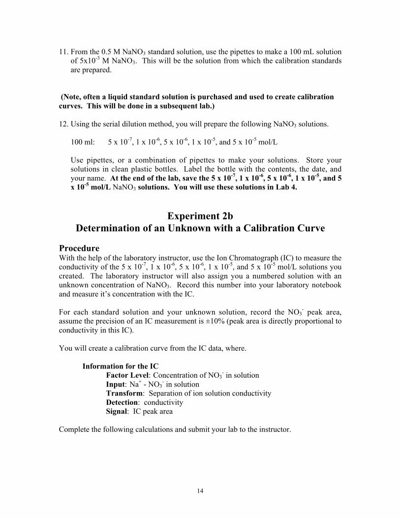
11. From the 0.5 M NaNO3 standard solution, use the pipettes to make a 100 mL solutionof 5x10-3 M NaNO3. This will be the solution from which the calibration standardsare prepared.

(Note, often a liquid standard solution is purchased and used to create calibrationcurves. This will be done in a subsequent lab.)

12. Using the serial dilution method, you will prepare the following NaNO3 solutions.

100 ml: 5 x 10-7, 1 x 10-6, 5 x 10-6, 1 x 10-5, and 5 x 10-5 mol/L

Use pipettes, or a combination of pipettes to make your solutions. Store yoursolutions in clean plastic bottles. Label the bottle with the contents, the date, andyour name. At the end of the lab, save the 5 x 10-7, 1 x 10-6, 5 x 10-6, 1 x 10-5, and 5x 10-5 mol/L NaNO3 solutions. You will use these solutions in Lab 4.

Experiment 2bDetermination of an Unknown with a Calibration Curve

ProcedureWith the help of the laboratory instructor, use the Ion Chromatograph (IC) to measure theconductivity of the 5 x 10-7, 1 x 10-6, 5 x 10-6, 1 x 10-5, and 5 x 10-5 mol/L solutions youcreated. The laboratory instructor will also assign you a numbered solution with anunknown concentration of NaNO3. Record this number into your laboratory notebookand measure it’s concentration with the IC.

For each standard solution and your unknown solution, record the NO3- peak area,

assume the precision of an IC measurement is ±10% (peak area is directly proportional toconductivity in this IC).

You will create a calibration curve from the IC data, where.

Information for the ICFactor Level: Concentration of NO3

- in solutionInput: Na+ - NO3

- in solutionTransform: Separation of ion solution conductivityDetection: conductivitySignal: IC peak area

Complete the following calculations and submit your lab to the instructor.

15

Calculations

1. Using ANOVA, calculate the slope (m) and y-intercept (b) for your calibration curve.Define your calibration curve as a linear function. Show all math.

2. Plot the calibration curve for your 5 standard NaNO3 solutions.x-axis = Factor Level = [NO3

-] in units mol/Ly-axis = Average Response = conductivity (peak area)

3. Using the Excel trendline function, generate the "best fit" linear trendline, trendlineequation, and standard deviation for your trendline. (You can use other software ifyou wish).

4. Using your calculated linear function and the trendline equation in Excel, calculatethe concentration of NO3

- in your unknown solution.

5. Calculate the absolute uncertainty and the relative (%) uncertainty for theconcentration of your unknown solution.

Questions1. Does the "best fit" trendline equation in Microsoft Excel match the linear calibration

equation you calculated using ANOVA? Explain why they are the same or different.(1 pt)

2. Say you must prepare a standard solution of 50 ml of 0.1 M CaCl2. How much CaCl2

solid should you dissolve into 50 ml to make the solution? (2 pts)

3. You have 100 ml of standardized 0.01 M H2SO4. You need to make a series of dilutesulfate solutions from the 0.01 M solution.

(a) How many ml of 0.01 M H2SO4 is required to make 100 ml of 0.002 M H2SO4?(1 pt)

(b) How many ml of 0.01 M H2SO4 is required to make 100 ml of 0.002 normalH2SO4? (1 pt)

(c) You transfer a 25-ml aliquot of the 0.01 M H2SO4 solution to a 500-mlvolumetric flask, then dilute to the mark. You then transfer a 25-ml aliquot ofthis solution to a 100-ml volumetric flask, then dilute to the mark. What is theconcentration of SO4

2- in your final solution in ppm units? (2 pts)

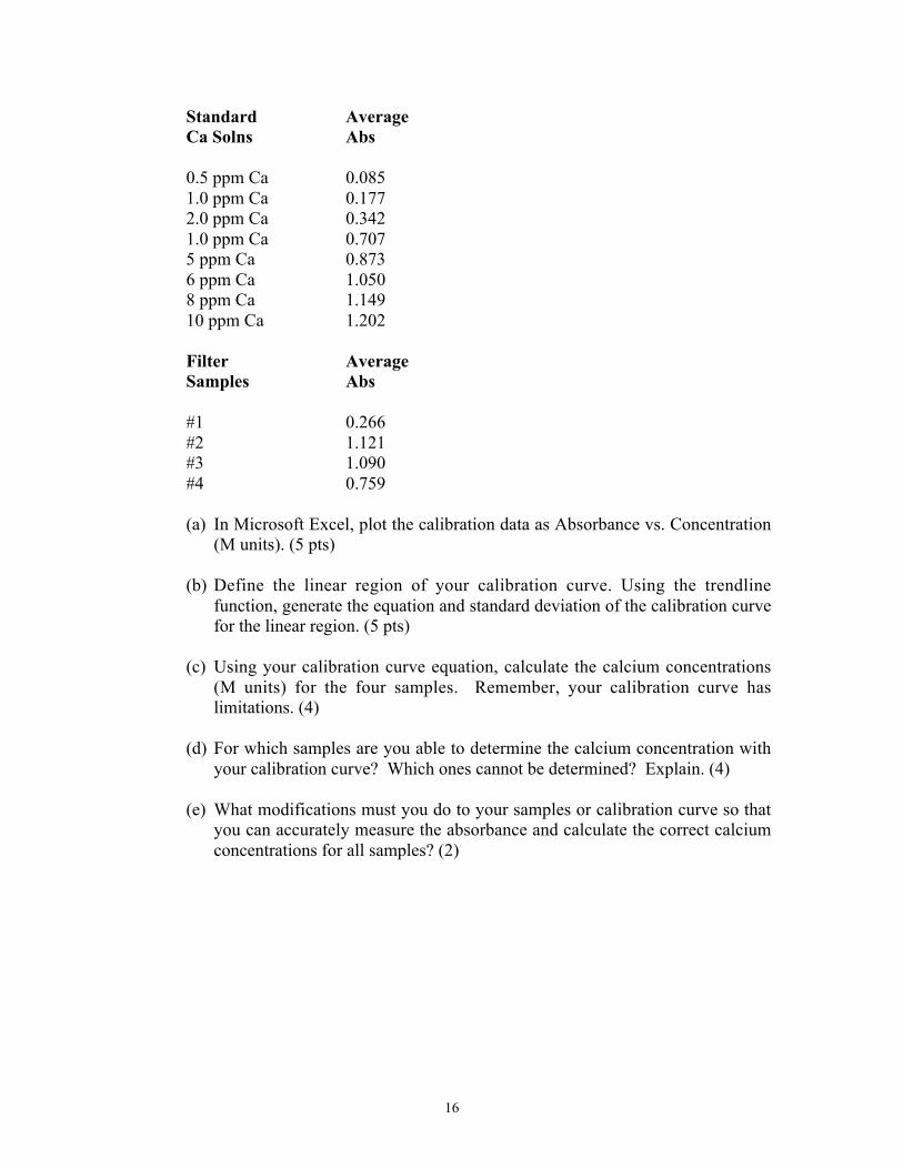
4. You are to measure the calcium ion concentration associated with aerosol particlescollected onto 4 filter samples using flame atomic absorption spectrophotometry asthe detector. You prepare 8 standard solutions for your calibration curve. Thefollowing data was collected.

16

Standard AverageCa Solns Abs

0.5 ppm Ca 0.0851.0 ppm Ca 0.1772.0 ppm Ca 0.3421.0 ppm Ca 0.7075 ppm Ca 0.8736 ppm Ca 1.0508 ppm Ca 1.14910 ppm Ca 1.202

Filter AverageSamples Abs

#1 0.266#2 1.121#3 1.090#4 0.759

(a) In Microsoft Excel, plot the calibration data as Absorbance vs. Concentration(M units). (5 pts)

(b) Define the linear region of your calibration curve. Using the trendlinefunction, generate the equation and standard deviation of the calibration curvefor the linear region. (5 pts)

(c) Using your calibration curve equation, calculate the calcium concentrations(M units) for the four samples. Remember, your calibration curve haslimitations. (4)

(d) For which samples are you able to determine the calcium concentration withyour calibration curve? Which ones cannot be determined? Explain. (4)

(e) What modifications must you do to your samples or calibration curve so thatyou can accurately measure the absorbance and calculate the correct calciumconcentrations for all samples? (2)