Lab 1: The Bipolar Junction Transistor (BJT): DC and AC ...nofong/ELEC3509/2011F_lab1.pdf · Lab 1: The Bipolar Junction Transistor (BJT): ... AC Characteristics Introduction

ELEC 3509 Electronics II Lab 1

Lab 1: The Bipolar Junction Transistor (BJT): DC and AC Characterization

Schedule for this lab: Day 1: BJT DC Characteristics Day 2: BJT AC Characteristics Introduction

When designing a circuit, it is important to know the properties of the devices that you will be using. This lab will look at obtaining important device parameters from a BJT. Although many of these can be obtained from the datasheet, datasheets may not always include the information we want. Even if they do, it is also useful to perform our own tests and compare the results. This process is called device characterization. In addition, the tests you will be performing will help you get some experience working with your tools so you don’t waste time fumbling around with them in future labs.

In day 1, you will be looking at the DC characteristics of your transistor. This will give you an idea of what the I‐V curves look like, and how you would measure them. You will also have to build and test a current mirror, which should give you an idea of how they work and where their limitations are.

In day 2, you will look at the AC characteristics. You will learn how to measure medium and higher frequency measurements, and how to calculate useful transistor characteristics from them.

Day 1: BJT DC Characterization Background:

After reading the following elementary introduction to the BJT, be sure to read Sedra and Smith, “Micro‐Electronic Circuits” 4th edition, SS4 pp. 221‐253, (5th edition, SS5 377‐401, 421‐436), ending with the D.C. analysis of transistor circuits, SS4 pp. 509‐511 (SS5 567‐569), on the current mirror. You are responsible for knowing this material regardless of whether or not you actually choose to read it.

The BJT is a three‐terminal semiconductor device containing two PN junctions. If checked with an ohm‐meter it appears to be two diodes of opposite polarity connected in series. However, unlike two series diodes, the BJT can be used to amplify. This is because the base is small enough to allow the two sets of PN‐junctions to interact with each other. There are two basic types of BJT, as illustrated in Figure 1.1.

The npn BJT is similar to the pnp device, but with the n and p regions exchanged. There should be a diode‐like behavior between the B‐E and B‐C terminals.

BJT Operating Regions:

Figure 1.2 shows an example of an I‐V curve of a NPN BJT transistor. As its name would imply, an I‐V curve plots the device current of the device against a sweep of terminal voltage. Figure 1.2 shows an example of collector current as the collector‐emitter voltage is changed, with a separate curve for different base currents. This family of curves is organized by base current since the diode‐like characteristics of the current vs. base‐emitter voltage would make the voltages of each curve very similar (and highly susceptible to process variations). Figure 1.3 shows the opposite type of curve, with a plot of collector current as the base‐emitter voltage is swept. The collector‐emitter voltage is not changed as this does not affect the family of curves significantly. This curve doesn’t give as much insight as the first curve, but is shown as a comparison (more information could be obtained if ICE was plotted on a log scale instead of a linear scale, but is still not as useful).

BJTs, like all transistors, are non‐linear. The non‐linear properties are what make it useful as an amplifier or switch, but as you will find in higher level courses, non‐linear devices are a pain to analyze. Fortunately, we can treat a BJT as a linear device as long as its current/voltage characteristics remain in one of a few confined regions. Figure 1.2 shows the 3 main regions of operation of the BJT. A fourth one exists (reverse active) but is not used in practice due to its poor properties. The very same semiconductor conditions that give high gain in the normal active region are the same ones that cause low gain in the reverse active region.


(a) Basic structure. (b) Symbol. (c) Practical structure. E=Emitter B=Base C=collector

Figure 1.1 BJT (PNP top figure and NPN bottom figure).

Figure 1.2: Plot of the I‐V curves of an example transistors sweeping VCE for different IB showing 3 regions of operation of the BJT


Figure 1.3 Plot of an I‐V curve of an example transistor sweeping VBE with a fixed VCE

(i) Saturation Region

In this region, both BIT junctions are forward biased. VCE is small, e.g. 50‐100 mV, but quite large collector and base currents (Ic & IB) can flow. This region is not used for amplification. There is a low resistance between the C and E terminals: the BJT acts like a closed switch. Figure 1.4 shows an actual circuit of a BJT in saturation and the small signal equivalent (that is, the linear model) of the circuit.

An actual circuit with an NPN BJT Approximate equivalent circuit.

Figure 1.4 Saturation region (ii) Active Region

Here the B‐E junction is forward biased but the B‐C junction is reverse biased. Because the two junctions are very close together, the emitter "emits" carriers which shoot across the central base region and are "collected" by the collector region. This flow of carriers manifests itself externally as a relatively large collector current Ic. This process is strongly influenced by the external injection of a much smaller current IB into the base region.

This lets the collector current to be controlled almost completely by the base‐emitter junction voltage, and is nearly independent on the collector node voltage (a very useful result). As the collector/emitter current ratio is dependent on fixed semi‐conductor parameters, we can define the BJT current gain:


Figure 1.5 shows an actual BJT operating in the active region and the small signal equivalent model. Do not confuse this with a MOSFET in saturation, which behaves similarly to the BJT in the active region.

An actual circuit with an NPN BJT Approximate equivalent circuit for silicon BJT.

Figure 1.5 Active region, B‐E diode is forward biased (iii) Cutoff Region

If both the junctions are reverse‐biased, only very small reverse leakage currents can flow across them. No gain is available in this mode, and there is a high resistance between the C and E terminals.

The small signal circuit model is not shown: it is just an open circuit between all 3 nodes.


Part 1: Diode‐Like behavior of BJT Junctions, and BJT Type Experiment: Using an ohmmeter on the "diode" range, measure the forward and reverse "resistances" of the B‐E, B‐C and C‐E junctions of a 2N3904 transistor, shown in Fig. 1.6. The Digital Volt Meter (DVM) on the "diode" range actually forces an output current of 1mA from its "V" terminal, and then measures the voltage developed between the "V" and common terminals. Thus, the DVM can directly measure the forward voltage drop of PN junction under 1mA of bias.

Note the orientation of the device as seen in Figure 1.6: it is a very common mistake to switch the emitter and collector terminals. Another common mistake is to confuse a PNP transistor for an NPN transistor or vice‐versa.

Figure 1.6 Lead Configuration of a 2N3904 Transistor. The lead configuration for the 2N3906 is exactly the same.

There should be diode‐like behavior between the B‐E and B‐C terminals, but not between the C‐E terminals

in either direction. Any other behavior usually indicates a damaged BJT. Of course, it is possible for a BJT to be damaged but still pass this test. Remember to record which meter lead is connected to which transistor terminal. By measuring the polarity of the voltage appearing across the ohmmeter leads, determine whether the 2N3904 is a pnp or npn type. Do the same for the 2N3906 transistor. Report: For your report, show a table showing the results you see from this test. Is there anything that you see that would be considered unusual?

Part 2: BJT IC vs. VCE Characteristic Curves ‐ Point‐by‐Point Plotting

Figure 1.7 Test circuit for Part 2

For this section, you will generate a plot similar to Figure 1.2 by plotting IC vs VCE with a fixed value of IB. Instead of doing several curves with varying values of IB, instead you only need 1‐ for this curve IC in the active region should be 1 mA. R2 is a potentiometer. It allows variable resistances both above and below the node, but the entire resistance from the top to the bottom is fixed at 1kOhm. This allows the base voltage to be adjusted by fine increments. Prelab: For this part, determine appropriate values of R1, RB and RC. You will need to justify these choices in your report with good reasons. Obviously there will be many possible values of RC, with each representing a different


VCE. Choose at least 5 values in the active region and another 5 or more values in the saturation region. Show the expected VCE for each resistance.

As a hint, for these calculations, keep in mind that VBE is around 0.7 V in the active region, VCE,sat is 0.5V, beta is around 150 and that the voltage drop across any resistor should be at least 0.25 V to be able to measure it accurately. In addition, the current flowing in the left branch should be much greater than the base current and the potentiometer should be in its middle range (to give us more freedom in dealing with component variations). You can assume the potentiometer is set somewhere in its middle region (500 ohms on both sides). Experiment: Using your calculated resistance values, assemble the circuit and measure IB. With the device in the active region, adjust the potentiometer so that IC is around 1mA. Then, keep this value of IB fixed and measure IC, VBE and VCE as you change the values of RC. Report: Plot the IC‐VCE line for the base current that was used. Determine the IC/IB current ratio for the transistor at each point.

Plot VBE vs. VCE. Does VBE change very much as VCE is changed? Why? What happens to this current ratio when the transistor goes into saturation?

From your plot, determine the value of beta and a value for the Early voltage VA.

Part 3: The Current Mirror

In network analysis, you have encountered two types of sources: fixed voltage and fixed current courses. With a voltage source, the voltage across the terminals is always a fixed value, while with a current source, the current flowing through the source is always a fixed value. While it is fairly easy to implement a fixed voltage source (e.g. a voltaic cell), implementing a current source is more difficult.

Your textbook and your notes show examples of a circuit called a current mirror which is the easiest implementation of a current source. A current mirror typically has two or more branches‐ in one branch (known as the reference branch) a fixed, known current flows, which can be controlled by adjusting a potentiometer, by adjusting some controllable switches or by a self‐correcting circuit such as a band‐gap generator. The other branch has a current flowing through them which is a direct multiple of the reference branch: ratios of 1:1 to 1:4 are common, and higher ratios are possible if less accuracy is needed.

An NPN current mirror with emitter degeneration resistors is shown in Figure 1.8. The emitter resistors, RE1 and RE2, reduce the effect that mismatches in VBE between the two discrete transistors have on the matching of the output current to the reference current. These resistors can also be conveniently used to alter the ratio between the two currents. Different permutations of this circuit exist which allow the mirror to operate at a wider output voltage range, or increase output impedance.


Figure 1.8 The Current Mirror and Test Circuit.

Prelab:

Given the circuit in Figure 1.8, derive a formula for the output current only in terms of RE1, RE2, VBE1, VBE2, β1, β2, RRef, RL, and VCC. Assume VBE1=VBE2 , β are both very large and the Early Voltage is negative infinity.

With RE1 set to 1kOhm, pick a value of RE2 so that the current is mirrored in a 1:1 ratio and a value of RE2 so that the current is mirrored in a 1:4 ratio. Choose an appropriate value of RRef (remember that the base is shorted to the collector) so that the reference current is approximately 0.75 mA.

Determine the maximum value of RL for which the current mirror will still be able to deliver the necessary amount of current. Keep in mind that the behavior of the transistor changes if it enters a different region of operation. Choose 10 values for RL, 5 that show the range of load resistances over which the current mirror operates and 5 that show where the current mirror fails. Show the expected current and output voltage for each load resistance.

Design a PNP current mirror such that it can be connected to the NPN current mirror as can be seen below. Note that the PNP current mirror may have other connections not seen in the figure (such as a connection to power). The PNP current mirror should mirror its reference current in a 1:1 ratio.

Figure 1.9 Schematic of the NPN current mirror connected to the PNP current mirror with test circuit


Experiment:

Construct the NPN current mirror as shown in Figure 1.8 and test the circuit with the set of loads you picked out in the prelab. For each load, measure the output voltage (Vout), and calculate the current flowing through the load resistor.

Modify the circuit to obtain a 1:4 current multiplier and measure the current flowing through a few different loads (at least 4) to show that the current mirror is in fact still acting as a current source with the correct output current.

Construct the PNP current mirror that you designed and connect it to the NPN current mirror as shown in Figure 1.9. Note that the load resistance of the NPN current mirror is replaced by the reference branch of the PNP current mirror. Measure the current flowing through a few loads (at least 4) to show that the current mirror is in fact still acting as a current source with the correct output current. Report:

Make a new derivation for the formula for the output current only in terms of RE1, RE2, VBE1, VBE2, β1, β2, RRef, RL, and VCC. This time, do not make any assumptions about them: for instance, you cannot assume VBE1=VBE2 or that any of the β values are large. You may assume that the Early Voltage is negative infinity. A good starting point is to find an equation for the current flowing through the left branch.

Following this, assume that VBE1=VBE2=0.7, VCC=15V, β1 and β2 are both infinite and simplify your equation accordingly. You should get the same expression as you did in your prelab.

With your measurements from your 1:1 mirror, make 2 plots‐ one showing output current vs. load resistance and one showing output current vs. output voltage. From your second plot, determine what the output impedance is. As a hint, keep in mind that a current mirror can be modeled as an ideal current source in parallel with a large resistance (which is its output resistance). Note that figuring out how to get the output impedance from the plot is part of this question.

Make another plot showing the output current vs. load resistance for your 1:4 mirror and another one for your PNP mirror.

Comment on the first transistor‐ with the base and collector shorted out, what two‐terminal device does it resemble the closest? With the transistor configured in this way, can it enter the saturation region of operation? If so, under what conditions? If not, why not?

Consider the range of loads over which the 1:1 mirror can deliver its rated current. How would you expect this range to change with the 1:4 region and why?


Day 2: BJT AC Characteristics Purpose:

Previously, we measured some of the DC characteristics of a BJT transistor. In this part of the lab, we will look at the AC operation of the transistor. In this course and in other courses, you may have encountered names such as Rpi or gm when performing calculations. These parameters are specific to the device (and the device model) that you are using. In order to compare devices of different types, we use a different set of network parameters. In this lab, you will become familiar with the h‐parameters and the hybrid‐pi model of the bipolar junction transistor.

Introduction:

Before doing this exercise, read Sedra and Smith, "Micro‐Electronic Circuits", SS4 pp. B4‐B5 (SS5 B4‐B5), on the h‐parameters, and SS4 pp. 259‐261, Ex.4.9, pp. 262 and pp. 322‐325, (SS5 448‐449, Ex. 5.14 p 450, and pp. 487‐490) on the hybrid‐pi models for BJTs. Part 4: The Transistor's h‐Parameters and Bandwidth:

The four h‐parameters describe all of a transistor's small‐signal ac characteristics for a given set of dc bias conditions, at one frequency. At low to medium frequencies, they are independent of frequency. The four parameters are:

hie: the ac input impedance with the output short‐circuited hoe: the output admittance with the input open‐circuited hfe: the ac forward current gain with the output short‐circuited, and hre: the reverse, or feedback, voltage ratio with the input open‐circuited

The second subscript, e, indicates that these parameters are measured with respect to the emitter, the

emitter being the terminal common to both the input circuit and the output circuit. All but the last h‐parameter will be measured in this exercise, the last one being so close to zero as to be practically unobservable using the equipment of the ELEC 3509 laboratory.

The one other transistor parameter of major interest is its unity‐gain bandwidth, fT, the frequency at which

its ac current gain is reduced to one. In most cases, equipment bandwidth limitations prevent the direct measurement of fT for any active device, so it is usually determined by extrapolating results at lower frequencies. In this case, this can be done by observing the low‐frequency current gain hfe, and by measurements of the beta cut‐off frequency, fβ, the frequency at which hfe drops by 3dB; fT is the product of fβ and hfe (see Figure 1.10).

Prelab: Using Figure 1.14 as a starting point, derive an equation for all of the h parameters. Leave all

transistor parameters (gm, Cpi, etc.) as variables‐ don’t substitute any values for them.


Figure 1.10 A plot showing current gain vs frequency. Here, the fT can be seen directly to be 1 MHz, but can be calculated by multiplying hfe=100 by fβ=10kHz.

Part 4 (a): Dc‐Biasing Circuit To establish a set of dc bias conditions on the BJT that will allow its use as an ac amplifier whose

characteristics can be determined, set up the circuit shown in Figure 1.11. Be sure to use the same transistor that was partially characterized in part 2. Use a value of RC to maintain a VCE around 7.5 V and whatever values of R1 and RB you used in Day 1.

Figure 1.11 DC Bias circuit for the AC characterization tests

‐10

0

10

20

30

40

50

1 10 100 1,000 10,000 100,000 1,000,000 10,000,000

Small signal AC Current gain Ic/IB (dB)

Frequency (Hz)

Transistor current gain vs frequency

fβ=10 kHz

hfe =40dB=100A/A


Adjust the potentiometer to set IC to 1 mA, and measure VCE so that during the subsequent tests the dc collector conditions in the circuit will be known.

Part 4 (b): Ac‐Coupling of Input and Output Signals

In addition to the circuit shown in Figure 1.11, add the additional circuitry shown in Figure 1.12 after measuring the values of RS and RL. This additional circuitry couples AC test signals into and out of the DC‐biased transistor circuit, which is the Device Under Test, or DUT. It is the AC characteristics of the DUT that will be determined in the following sections of this exercise, by related measurements on the DUT’s input and output Fig, 1.13 represents a "black‐box" view of the D.U.T. in the test circuit.

In your report, explain the purpose of the capacitors C1 and C2, making sure to identify what would happen if they were absent.

Figure 1.12 Ac Test Circuit for the Biased BJT

Be certain to observe the POLARITY of the electrolytic capacitors when connecting them; if reversed, they will conduct dc current, and will permanently ruin them.

Figure 1.13 "Black‐Box" View of the DUT in the AC Test Circuit.


Part 4 (c): The AC Input Impedance, hie, and the ac Forward Current Gain, hfe

Note: See appendix A at the end of this lab for more information about making AC measurements. Experiment: Connect the signal generator to the circuit and set the signal source to provide a 1 kHz sinusoid, and use the source's "low‐amplitude" output connector. Set the AC base current, ib, to 0.5 µA RMS by adjusting the output level of the source while using the multimeter to monitor vib across RS (make sure to measure it using the AC mode). Note that the multimeter’s output is RMS, not peak‐peak or peak. The input impedance of the multimeter is high enough that its effect on measurements in this circuit can be ignored at low frequencies.

By observing the oscilloscope, ensure that the circuit is not distorting the signal‐ this is a qualitative observation, not a quantitative one (we’ll talk more about this later). Next, using the multimeter, measure vbe and vo. Again the multimeter’s impedance can also be ignored since the circuit impedances are small.

Finally, calculate the ac input impedance:

and the ac forward current gain:

where

The expected range of results for hie and hfe can be found in the attached specifications for the 2N3904 transistor.

Note that the output short‐circuit condition properly required for measuring hie and hfe is only approximately met by the 100 ohm load resistance that was used in the test circuit. However, the error that it produces here is small. (In later calculations of the hybrid‐pi parameters, the fact that there exists an AC output voltage will have to be taken into account).

Report: In your report, show your results and calculations. Describe why the value of the load resistor cannot be made to be zero.


Part 4(d): The AC Output Admittance, hoe, and the AC Reverse, or Feedback, Voltage Ratio, hre Since we are dealing with very low frequencies, the ac output admittance, hoe, can be found from the DC

characterization you performed in day 1. In this case, it is the slope of the IC vs. VCE characteristic curve at the point of dc operation. Use the IC vs. VCE graph from part 2 to find hoe, ignoring the fact that IC may not be exactly the same in the graph as it is in this part of the experiment, but it will be close. The units of hoe are amps/volt, or mhos. Express the admittance in µmhos, as this is usual since its value will be quite small. The expected range of hoe can be found in the attached specifications.

Note that in general, AC parameters cannot be found from looking at the DC I‐V curves, although this is usually ok if we are not working at very high frequencies.

The ac feedback voltage ratio, as previously mentioned, is too small to measure in the ELEC 3509 1aboratory. Therefore, take hre = 0.

Part 4 (e): The Unity‐Gain Bandwidth, fT, and the Beta Cut‐Off Frequency, f�

Prelab: Using Figure 1.14 as a starting point, derive an equation for fT. You can make some assumptions: assume Rx=0, Rμ=infinity, Cμ=0, RO=infinity. Note that the conditions for measuring fT requires a shorted output (you can use a resistor of arbitrarily small value if that helps) and that the definition of fT is the frequency where the magnitude current gain (output AC current divided by input AC current) is exactly 1 (phase shifts are fine).

Experiment: For this part of the experiment set the AC ib set to approximately 0.5 µA RMS at 1 kHz. Use the

oscilloscope method described earlier to measure the voltage across the resistance RS and RL. To keep you from having to change too many setting in the oscilloscope, you can just short one of the probes to ground when measuring the voltage across RL. From this, calculate the current gain‐ this is your hfe.

Continue to make these measurements as you increase the frequency‐ you will need enough data points to make a plot like Figure 1.10. Increasing the frequency by factors of 2‐3 per measurement should be ok. Although you won’t be able to measure the point where the current gain drops to 0 dB, you must be able to reach and exceed the point where the current gain drops to 71% of its low frequency value (a 3 dB drop). You can find this exact location by interpolation. Note that you cannot assume that the signal generator voltage will remain constant over frequency‐ you must re‐measure the voltage across R4 each time. This is your fβ

From these values, calculate fT: fT = hfe × fβ

Change the DC bias conditions so that the DC IC is 0.5 mA and find fT again. Change RC to keep VCE around

7.5V. Repeat with IC=2 mA. You do not need to make a plot of current gain/frequency for these two‐ just find hfe and f� and as a result, fT.

Report: For the 1 mA bias condition, plot current gain (in dB) as a function of frequency (in a log scale). On the plot, show your values of hfe and fβ.


Part 5: The BJT High‐Frequency Hybrid‐Pi Model

Fig. 1.14 The High‐Frequency Hybrid‐Pi Model of a BJT. Report: Figure 1.11 shows the high‐frequency hybrid‐pi model of a BJT. The equations given below define its elemental values in terms of the previously measured circuit parameters. For your report, calculate all of these values, and make a copy of them as they will be needed for designing the amplifiers of the first project.

Eqs. (1.5)

Eqs. (1.6)

rx = hie ‐ rπ (If through experimental error rx becomes negative, then set rx = 0. ) Eqs. (1.7)

Eqs. (1.8)

Eqs. (1.9)

Eqs. (1.10)

C� = CBCjunction + Cboard ≈ 2pf + 2pf = 4pf Eqs. (1.11)


Eqs. (1.12)

Notice that Eq. (1.12) is modified to account for vo ≠ 0. If Cπ negative set Cπ = 0. Note that these equations are for a model of the BJT installed on the prototype board as they take into

account the effect of board inter‐connection capacitances. This model is useful as it accurately represents the BJT as it will be used in the circuits of Lab 2

The 2N3904 transistor specifications are provided in the following page.



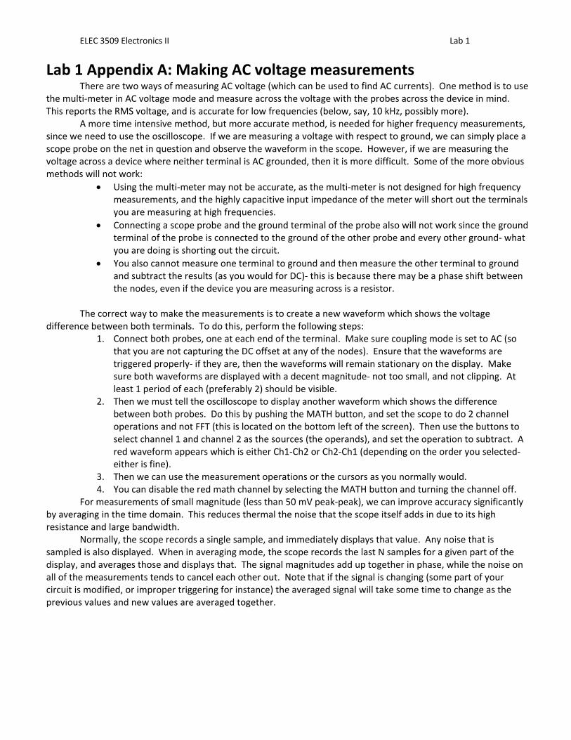
Lab 1 Appendix A: Making AC voltage measurements There are two ways of measuring AC voltage (which can be used to find AC currents). One method is to use

the multi‐meter in AC voltage mode and measure across the voltage with the probes across the device in mind. This reports the RMS voltage, and is accurate for low frequencies (below, say, 10 kHz, possibly more).

A more time intensive method, but more accurate method, is needed for higher frequency measurements, since we need to use the oscilloscope. If we are measuring a voltage with respect to ground, we can simply place a scope probe on the net in question and observe the waveform in the scope. However, if we are measuring the voltage across a device where neither terminal is AC grounded, then it is more difficult. Some of the more obvious methods will not work:

Using the multi‐meter may not be accurate, as the multi‐meter is not designed for high frequency measurements, and the highly capacitive input impedance of the meter will short out the terminals you are measuring at high frequencies.

Connecting a scope probe and the ground terminal of the probe also will not work since the ground terminal of the probe is connected to the ground of the other probe and every other ground‐ what you are doing is shorting out the circuit.

You also cannot measure one terminal to ground and then measure the other terminal to ground and subtract the results (as you would for DC)‐ this is because there may be a phase shift between the nodes, even if the device you are measuring across is a resistor.

The correct way to make the measurements is to create a new waveform which shows the voltage

difference between both terminals. To do this, perform the following steps: 1. Connect both probes, one at each end of the terminal. Make sure coupling mode is set to AC (so

that you are not capturing the DC offset at any of the nodes). Ensure that the waveforms are triggered properly‐ if they are, then the waveforms will remain stationary on the display. Make sure both waveforms are displayed with a decent magnitude‐ not too small, and not clipping. At least 1 period of each (preferably 2) should be visible.

2. Then we must tell the oscilloscope to display another waveform which shows the difference between both probes. Do this by pushing the MATH button, and set the scope to do 2 channel operations and not FFT (this is located on the bottom left of the screen). Then use the buttons to select channel 1 and channel 2 as the sources (the operands), and set the operation to subtract. A red waveform appears which is either Ch1‐Ch2 or Ch2‐Ch1 (depending on the order you selected‐ either is fine).

3. Then we can use the measurement operations or the cursors as you normally would. 4. You can disable the red math channel by selecting the MATH button and turning the channel off.

For measurements of small magnitude (less than 50 mV peak‐peak), we can improve accuracy significantly by averaging in the time domain. This reduces thermal the noise that the scope itself adds in due to its high resistance and large bandwidth.

Normally, the scope records a single sample, and immediately displays that value. Any noise that is sampled is also displayed. When in averaging mode, the scope records the last N samples for a given part of the display, and averages those and displays that. The signal magnitudes add up together in phase, while the noise on all of the measurements tends to cancel each other out. Note that if the signal is changing (some part of your circuit is modified, or improper triggering for instance) the averaged signal will take some time to change as the previous values and new values are averaged together.


To set the scope in averaging mode: 1. First make sure that the waveform you want to average is visible on the screen, is not too small or

clipping, is triggered properly, and has several periods visible. 2. Press the “Menu” key in the acquire section of the scope (the rightmost section). 3. The acquisition mode of the scope is on the right hand side of the display. To put the oscilloscope

in averagin, press select the “average” option on the bottom. To restore the scope into normal operation, use the “sample” option on the top. Ignore the two middle options for now, you won’t need them in this course.

4. When “Average” is selected, you can turn the dial on the top of the scope (the one next to the “select” and “coarse” buttons) to change the number of samples. Increasing the number of samples improves accuracy but takes longer‐ this is the tradeoff with all measurements. Realistically, only a few averages are necessary‐ accuracy goes up with the square root of the number of samples.

Note that when you make a change to the circuit, you will need to reset the scope’s built‐in memory, so

you don’t average the changed values with the previous values. You can do this by turning averaging off and then back on again. If your average is small enough, you don’t need to worry about this (the previous samples will be forgotten before you change the scope settings).

Documents

Lab 1: The Bipolar Junction Transistor (BJT): DC and AC ...nofong/ELEC3509/2011F_lab1.pdf · Lab 1: The Bipolar Junction Transistor (BJT): ... AC Characteristics Introduction