Embed Size (px)
Citation preview
Lab 1: Ensemble Fluorescence Basics
(Last Edit: Feb 18, 2016)
This laboratory module is divided into two sections. The first one is on organic fluorophores, and the
second one is on ensemble measurement of FRET (Fluorescence Resonance Energy Transfer)
I. Organic Fluorophores1
In this lab you will be measuring the absorption, emission, and lifetime of cyanine dyes (Cy3, Cy5
and Cy5.5). Once you are familiar with the instruments, you will measure the absorption, emission
and lifetime of three unknown samples to identify the fluorophore within the sample.
Objective:
1. Learn to take absorption spectra, emission spectra and lifetime measurement of fluorophores
2. Understand properties of organic fluorophores (resonance delocalization, cis-trans isomerism)
3. Be comfortable with pipetting as an essential basic for future labs
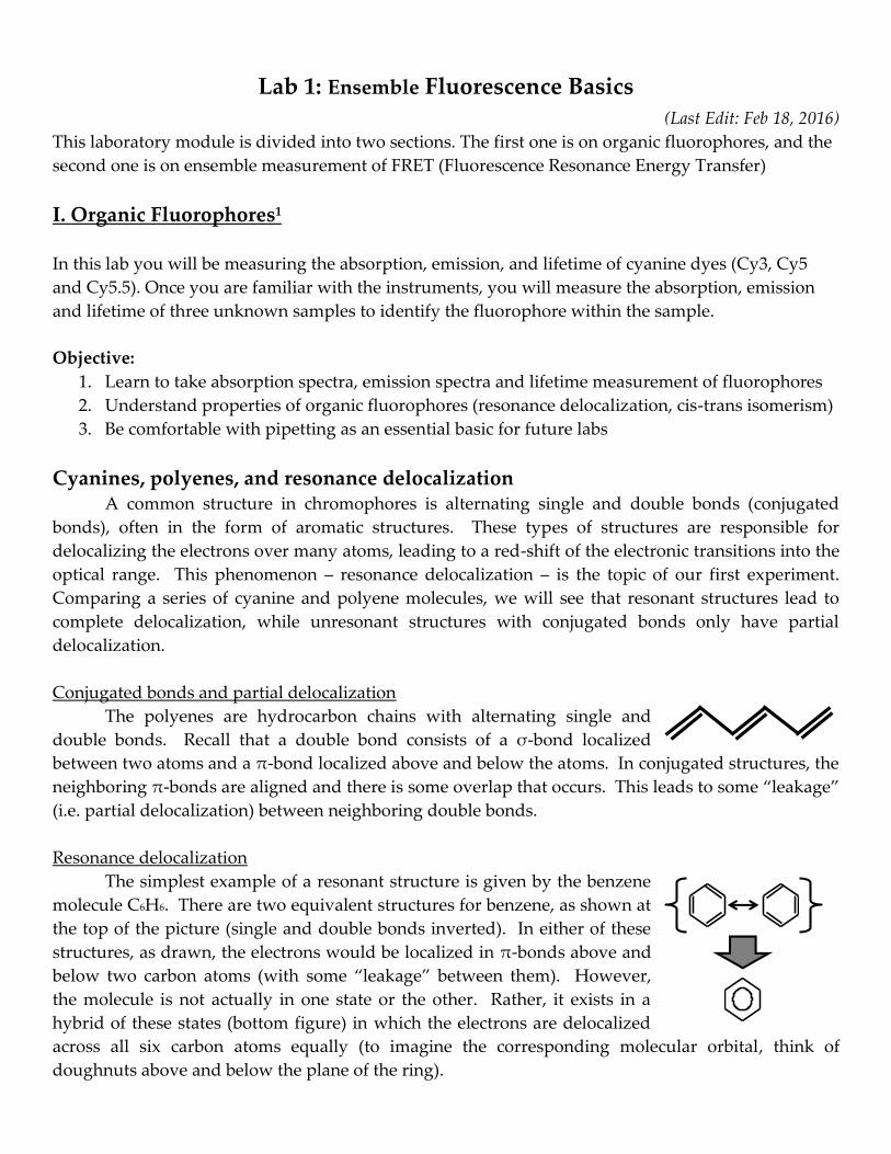
Cyanines, polyenes, and resonance delocalization A common structure in chromophores is alternating single and double bonds (conjugated
bonds), often in the form of aromatic structures. These types of structures are responsible for
delocalizing the electrons over many atoms, leading to a red-shift of the electronic transitions into the
optical range. This phenomenon – resonance delocalization – is the topic of our first experiment.
Comparing a series of cyanine and polyene molecules, we will see that resonant structures lead to
complete delocalization, while unresonant structures with conjugated bonds only have partial
delocalization.
Conjugated bonds and partial delocalization
The polyenes are hydrocarbon chains with alternating single and
double bonds. Recall that a double bond consists of a σ-bond localized
between two atoms and a π-bond localized above and below the atoms. In conjugated structures, the
neighboring π-bonds are aligned and there is some overlap that occurs. This leads to some “leakage”
(i.e. partial delocalization) between neighboring double bonds.
Resonance delocalization
The simplest example of a resonant structure is given by the benzene
molecule C6H6. There are two equivalent structures for benzene, as shown at
the top of the picture (single and double bonds inverted). In either of these
structures, as drawn, the electrons would be localized in π-bonds above and
below two carbon atoms (with some “leakage” between them). However,
the molecule is not actually in one state or the other. Rather, it exists in a
hybrid of these states (bottom figure) in which the electrons are delocalized
across all six carbon atoms equally (to imagine the corresponding molecular orbital, think of
doughnuts above and below the plane of the ring).

Fluorescein and pH dependence
Fluorescein is a bright green fluorophore
commonly used in fluorescence measurements. It has
two ionizable groups, –COOH and –OH. Depending on
the pH, it is found in four forms: dianion, monoanion,
neutral, and cation. In its dianionic form, it is a strong
absorber of visible light (ε490 ~90,000 L/mol-cm) and has a high fluorescence efficiency (φf > 90%).
This is because its structure is highly resonant, as shown in the figure, such that the electrons are
delocalized across the three rings at the top. Note that the bottom ring is not part of the
delocalization because the –COOH group causes steric interference and forces the ring to rotate out of
the plane of the other rings.
In its neutral form with the phenol and carboxylic groups protonated,
fluorescein’s emission degrades considerably and the absorption shifts toward
the blue and decreases. The reason is that the molecule is no longer in complete
resonance. The presence of the –OH group requires a proton to be transfered
from one side to the other in order to draw equivalent resonant structures.
Fluorescence lifetime A fluorophore excited by a photon will drop to the ground state
through radiative and non-radiative decay pathways.
Fluorescence lifetime is the average time a fluorophore spends in
the excited state before returning to ground state. When a solution
of fluorophore is excited with a pulse of light, an initial population
of fluorophores (n0) will be in the excited state. This excited state
population decreases with time with a constant decay rate ktot = kr
+ knr, where kr and knr are the radiative and non-radiative decay rate respectively. The fluorescence
intensity is proportional to the excited state population, and will decay exponentially following the
formula I(t) = I0 exp(-t/τ), where I(t) is the intensity at time t, I0 is the initial intensity and τ is the
lifetime that is the inverse of the total decay rate (τ = 1/ktot).
The lifetimes of organic fluorophores typically fall in the nanosecond regime. The fluorescence
lifetimes of cyanine dyes are marked by large non-radiative decay rate (knr ~10x larger than kr for
Cy3) caused by cis-trans photoisomerization2. Excited state of cyanine dyes undergoes
photoisomerization from trans to cis conformation. Once formed, the cis isomer undergoes thermal
back-isomerization to the ground state. This non-radiative process reduces the lifetime and quantum
yield of the dyes, and is strongly dependent on the microenvironment the dye is in. When attached to
single-stranded DNA (ssDNA) or double-stranded DNA (ssDNA), cyanine dyes may show two
component lifetimes indicative of multiple states arising from the DNA-dye interaction.

Experiment and Report
(1) You will each start with concentrated samples of Cy3, Cy5 and Cy5.5. Dilute each of them 400x (2
µL sample in 800 µL ddH2O) before taking any measurement. Cy5.5 has low solubility, so be sure to
shake the tube it is in well before pipetting.
(2) Measure the absorption spectra for the cyanine dyes from 450 to 750 nm (for operating instruction
and dilution protocols, see Appendix 2.1. It’s important to read beforehand!). Record the peak absorption
wavelength and the absorption in Table 1, and determine the concentration of the dyes in mol/L. To
calculate concentration, use the formula A = εcL, where A is the absorption measured at the peak
wavelength, ε is the extinction coefficient, c is the concentration and L is the path length. The relevant
extinction coefficients at the peak wavelength are εCy3 = 150,000 L/mol-cm, εCy5 = 250,000 L/mol-cm,
and εCy5.5 = 250,000 L/mol-cm. The path length of the cuvette is 1 cm. If your absorption spectrum is
too noisy to resolve the peak, increase the integration time (remember to take a new blank with the
same integration time).
(3) (2 pts) Measure the emission spectra of the cyanine dyes (Appendix 2.2). Use the values below for
the emission scan and excitation wavelength. Record the peak emission wavelength in Table 1 and
calculate the Stokes shift by subtracting the emission peak from the absorption peak.
Start Scan [nm] End Scan [nm] Excitation [nm] Time [s]
Cy3 540 700 510 0.2
Cy5 630 750 610 0.2
Cy5.5 670 800 650 0.2
Abs. Max [nm] Abs. Em. Max [nm] Stokes Shift [nm] Conc. [mol/L]
Cy3
Cy5
Cy5.5
Table 1. Absorption and emission peaks, stokes shifts, and concentrations of Cy3, Cy5 and Cy5.5
(4) (2 pts) Measure the lifetime of Cy3 attached to different substrates (Appendix 2.3). Use the
parameters below for each measurement. Record the lifetimes in Table 2. Each student will pick one
sample and share the data with the group. Measure up to the second lifetime component.
Ref. Dye Time Base Frequency Ref. Lifetime [ns] Filter [nm] Excitation [nm]
Erythrosin-B 1 10– 200 MHz 0.46 550 - 620 540
τ1 (ns) τ2 (ns) Fraction1 τave (ns)
Free-Cy3
Cy3-ssDNA
Cy3-dsDNA
Table 2. Lifetimes of Cy3 attached to different substrates

(5) (3 pts) Measure the absorption, emission and lifetime of one of the unknown samples given (A, B
and C). Each of you will pick one unknown and share the data with the group. Together with the
group, plan the parameters to be used for each measurement. First estimate the absorption max of the
sample from its color (the color you see are those not absorbed by the sample). Then estimate the
emission max (generally 20-30 nm greater than the absorption max). Knowing these peaks, you can
estimate the parameters needed for absorption, emission and lifetime measurement. Use the figure
below to help guide your decision. Summarize your plan in Table 3. Record your finding in Table 4
and use Table 5 to identify the unknown samples.
Ref. Dye Time Base Frequency Ref. Lifetime [ns] Filter [nm] Excitation [nm]
Erythrosin-B 1 10– 200 MHz 0.46 550 - 620 540
Fluorescein 1 4 – 90 MHz 4.0 500 - 520 480
Estimate Absorption Emission Lifetime
Abs.
Max
[nm]
Em.
Max
[nm]
Start
[nm]
End
[nm]
Start
[nm]
End
[nm]
Excit.
[nm]
Ref.
Dye
Ref.
τ [ns]
Filter
[nm]
Excit.
[nm]
A
B
C
Table 3. Plan for absorption, emission and lifetime measurement of unknown samples.
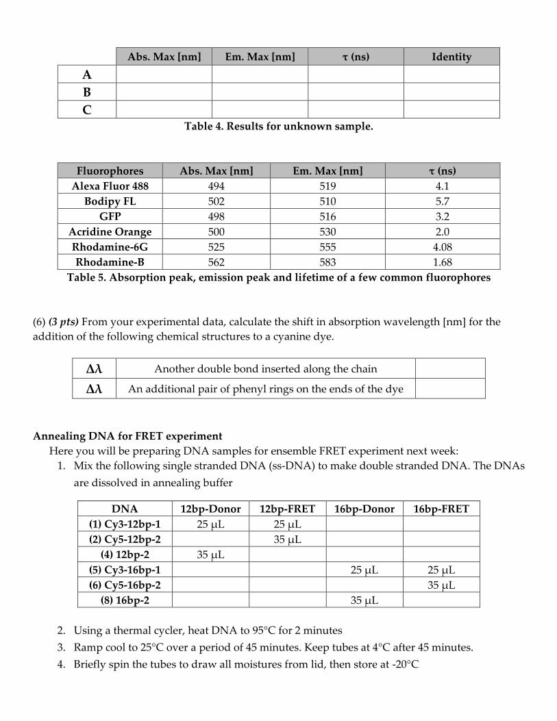
Abs. Max [nm] Em. Max [nm] τ (ns) Identity
A
B
C
Table 4. Results for unknown sample.
Fluorophores Abs. Max [nm] Em. Max [nm] τ (ns)
Alexa Fluor 488 494 519 4.1
Bodipy FL 502 510 5.7
GFP 498 516 3.2
Acridine Orange 500 530 2.0
Rhodamine-6G 525 555 4.08
Rhodamine-B 562 583 1.68
Table 5. Absorption peak, emission peak and lifetime of a few common fluorophores
(6) (3 pts) From your experimental data, calculate the shift in absorption wavelength [nm] for the
addition of the following chemical structures to a cyanine dye.
Δλ Another double bond inserted along the chain
Δλ An additional pair of phenyl rings on the ends of the dye
Annealing DNA for FRET experiment
Here you will be preparing DNA samples for ensemble FRET experiment next week:
1. Mix the following single stranded DNA (ss-DNA) to make double stranded DNA. The DNAs
are dissolved in annealing buffer
DNA 12bp-Donor 12bp-FRET 16bp-Donor 16bp-FRET
(1) Cy3-12bp-1 25 µL 25 µL
(2) Cy5-12bp-2 35 µL
(4) 12bp-2 35 µL
(5) Cy3-16bp-1 25 µL 25 µL
(6) Cy5-16bp-2 35 µL
(8) 16bp-2 35 µL
2. Using a thermal cycler, heat DNA to 95°C for 2 minutes
3. Ramp cool to 25°C over a period of 45 minutes. Keep tubes at 4°C after 45 minutes.
4. Briefly spin the tubes to draw all moistures from lid, then store at -20°C

(7) (4 pts) Identify the chemical structures in Cy3/Cy5 and Cy3.5/Cy5.5 corresponding to water
solubility, chemical reactivity (bioconjugation), major shifts in absorption (strongly resonant), and
minor shifts in absorption (moderately conjugated). Circle these parts in each molecule and label
their identity. Hints: Water is highly polar, so what would help something dissolve in it?
-electron system (the degree of conjugation) generally results in a red-shift of
the absorption and fluorescence as well as an increased quantum yield. So identify the parts of the
molecule that would cause small/large amounts of shift.
(8) (3 pts) Using the experimental data in Tables 8.2 and 8.4 on the next page, draw a rough (rough,
but still at least with evenly spaced ruling on the axes) sketch plotting the maximum absorption
wavelength, λ*abs [nm], versus the number of π-electrons, N, in the molecule for the polyenes and
cyanines with N = 4, 8, 12, and 16 (use experimental columns in Tables 8.2 and 8.4). Describe in your
own words with a couple sentences the graph and how the trends relate to resonance and electron
delocalization.
(9) (3 pts) Cyanine dyes have a relatively low quantum yield (~5 to 20%) compared to other
fluorophores like fluorescein and rhodamines (~70 to 95%). Give an explanation of this based on
what you have learned about the differences in chemical structures for these types of dyes.

(10) (3 pts) For the lifetime experiment, is the lifetime of Cy3 the same when conjugated to different
substrates? What are the possible factors that cause these differences? You can refer to the reference:
“Fluorescence Properties and Photophysics of the Sulfoindocyanine Cy3 Linked Covalently to DNA” for
helpful hints.
References: 1 Materials are partially adapted from PHYS 552 class by Prof. Robert Clegg 2 Sanborn, M. E., Connolly, B. K., Gurunathan, K., Levitus, M.. Fluorescence Properties and
Photophysics of the Sulfoindocyanine Cy3 Linked Covalently to DNA. J. Phys. Chem 2007
Part 2: Ensemble FRET
Introduction: In this lab, you will be doing FRET measurements using both steady-state and time-resolved
methods. You will measure the FRET efficiency and calculate the distance of two DNA samples with
different lengths (12 base-pair and 16 base-pair), and analyze the FRET efficiency using the sensitized
emission and lifetime method.
Background:
A. Samples: For the lifetime experiments, we will be using 12 and 16 base-pair oligo DNA from Integrated
DNA Technologies. One strand is labeled with the donor fluorophore Cy3, the other by the acceptor
fluorophore Cy5. For this lab, we will use singly-labeled and hybridized versions to estimate the
FRET efficiency.
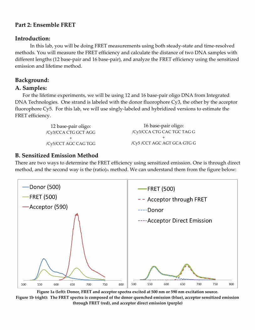
B. Sensitized Emission Method There are two ways to determine the FRET efficiency using sensitized emission. One is through direct
method, and the second way is the (ratio)A method. We can understand them from the figure below:
Figure 1a (left): Donor, FRET and acceptor spectra excited at 500 nm or 590 nm excitation source.
Figure 1b (right): The FRET spectra is composed of the donor quenched emission (blue), acceptor sensitized emission
through FRET (red), and acceptor direct emission (purple)
12 base-pair oligo: /Cy3/CCA CTG GCT AGG
+
/Cy5/CCT AGC CAG TGG
16 base-pair oligo: /Cy3/CCA CTG CAC TGC TAG G
+
/Cy5 /CCT AGC AGT GCA GTG G

Direct Method: With the direct method to calculate FRET efficiency, we compare the area under the red and
blue graph in Figure 1b. The FRET efficiency is simply the acceptor sensitized emission through FRET
(red graph) divided by the total FRET emission (donor + acceptor through FRET, or red + blue
graphs):
𝐸𝐹𝑅𝐸𝑇 =𝐼𝐴𝐷
𝐼𝐷𝐴 + 𝐼𝐴𝐷
where IAD is the acceptor emission through FRET and IDA is the donor quenched emission due to
FRET. The equation above assumes that the quantum yield of the donor and acceptor are the same. If
the quantum yields are different, as is the case for Cy3 and Cy5, we simply account for the different
quantum yield and use the equation below:
𝐸𝐹𝑅𝐸𝑇 =𝐼𝐴𝐷/𝑞𝐴
𝐼𝐷𝐴/𝑞𝐷 + 𝐼𝐴𝐷/𝑞𝐴
where qA and qD are the quantum yields of the acceptor and donor respectively.
(ratio)A Method: In the (ratio)A method, the emission of the acceptor is examined at two different excitation
wavelengths to determine the FRET efficiency. More specifically, the value (ratio)A is the emission of
the acceptor measured while exciting the donor divided by the emission of the acceptor undergoing
direct excitation. In Figure 1, (ratio)A is the acceptor extracted emission (red + purple graphs in Figure
1b) divided by direct acceptor emission at 590 nm (red graph in Figure 1a). The FRET efficiency (E) is
functionally dependent on (ratio)A and the extinction coefficients of our donor and acceptor taken at
specific wavelengths. This allows for a fairly straight-forward way to determine FRET efficiencies.
To use (ratio)A, we will need to measure the following spectra
1. Donor (500), the emission spectrum of donor-only sample collected at 500 nm excitation
wavelength
2. FRET (500), the emission spectrum of the FRET sample collected throughout at 500 nm
excitation wavelength. This will include emission from the donor because of direct excitation
by light at 500 nm wavelength, as well as from the acceptor because of (a) FRET and (b) the
small amount of direct excitation by light at 500 nm wavelength.
3. FRET (590), the emission spectrum of the FRET sample collected at 590 nm excitation
wavelength. This gives us a measure of the total number of acceptors in our sample.

The three spectra are shown in the figure below:
The numerator of the equation describing (ratio)A is the emission of the acceptor taken while exciting
the donor (undergoing FRET). To do this, we must subtract the donor emission from FRET(500). The
donor peak in Donor(500) must be re-scaled to match the donor peak in FRET(500). The denominator
of the (ratio)A is simply, FRET(590). The final equation is shown below,
(𝑟𝑎𝑡𝑖𝑜)𝐴 =[𝐹𝑅𝐸𝑇(500)] − [𝑁 ∙ 𝐷𝑜𝑛𝑜𝑟(500)]
[𝐹𝑅𝐸𝑇(590)]
where N = FRET-DA(500)/ Donor-DA(500). The spectra in the numerator and denominator will be
integrated to calculate (ratio)A. As mentioned previously, (ratio)A is functionally dependent of the
FRET efficiency of the system (E) as shown below,
(𝑟𝑎𝑡𝑖𝑜)𝐴 =𝜖𝐷(500) ∙ 𝐸 + 𝜖𝐴(500)
𝜖𝐴(590)
where εD(500) is the extinction coefficient of Cy3 at 500 nm, εA(500) is the extinction coefficient of Cy5
at 500 nm and εA(590) is the extinction coefficient of Cy5 at 590 nm.
We have made some simplifying assumptions about the fraction of labeling to arrive at this
simplified expression. A derivation of this will be provided with your lab report questions, but you
can motivate the formula by noting that the first term in the numerator is proportional to the FRET
enhanced acceptor emission (the FRET efficiency E times the amount of absorption by the donor) and
the second proportional to the amount of emission by direct excitation at D
EX which is proportional to
the amount absorbed by the acceptor. The denominator is proportional to the amount of light
absorbed by the excitation at A
EX and the subsequent acceptor emission.

C. Lifetime Method
Measuring the FRET efficiency of a particular system with lifetimes typically measures the
amount by which the lifetime of the donor shortens from the additional de-excitation pathway
present (while undergoing FRET). In other words, the additional pathway makes it more likely for
the excited donor molecule to return to the ground state, which therefore shortens the lifetime
(average time spent in the excited state). The relationship between the FRET efficiency (E), the
lifetime of the donor undergoing FRET (τDA) and the lifetime of the donor without the acceptor
present (τD) is written below
1 DA
D
E
To derive the equation, remember that the efficiency of energy transfer is the same thing as the
“quantum yield” of energy transfer. As discussed in lecture, the quantum yield of a given de-
excitation pathway (like FRET) is the rate of that pathway divided by the rates of all the pathways of
de-excitation available. Therefore, we can relate the FRET efficiency to the rates of the deactivation
pathways as shown,
T
T i
i T
kE
k k
In this equation, kT is the rate of energy transfer and ki are the rates of the other pathways present.
Next, to determine the relation between E and the lifetimes (τDA and τD), the rate constants in the
above equations need to be related to the lifetimes. The rate constants that describe the de-excitation
pathways for the molecule to leave the excited state are inversely proportional to the lifetime. This is
shown below, 1
D
i
i T
k
1DA
T i
i T
k k
With some algebra, the three previous equations can be used to derive the equation relating the FRET
efficiency (E) to the lifetime of the donor undergoing FRET (τDA) and the lifetime of the donor not
undergoing FRET (τD) as shown below.
1 DA
D
E
C. Fluorescent Anisotropy We will measure the anisotropy of free Cy3, Cy3-ssDNA and Cy3-dsDNA that we measure
lifetime for in the previous lab. The anisotropy value of a fluorophore is related to its rotational
lifetime φ through the relation:
𝑟 = 𝑟0
1 + 𝜏/𝜙
Where r is the observed anisotropy, r0 is the intrinsic anisotropy of the molecule, τ is the fluorescence
lifetime and φ is the rotational time constant. For our purposes, we can assume that r0 is 0.386.1
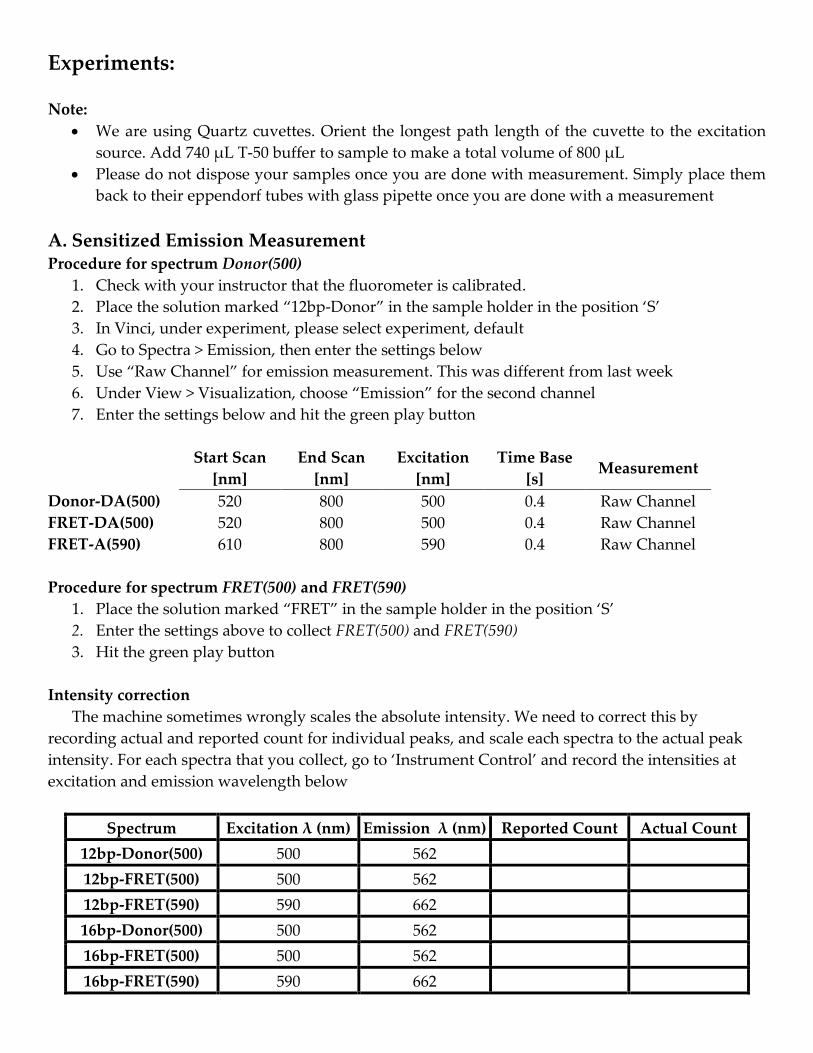
Experiments:
Note:
We are using Quartz cuvettes. Orient the longest path length of the cuvette to the excitation
source. Add 740 µL T-50 buffer to sample to make a total volume of 800 µL
Please do not dispose your samples once you are done with measurement. Simply place them
back to their eppendorf tubes with glass pipette once you are done with a measurement
A. Sensitized Emission Measurement Procedure for spectrum Donor(500)
1. Check with your instructor that the fluorometer is calibrated.
2. Place the solution marked “12bp-Donor” in the sample holder in the position ‘S’
3. In Vinci, under experiment, please select experiment, default
4. Go to Spectra > Emission, then enter the settings below
5. Use “Raw Channel” for emission measurement. This was different from last week
6. Under View > Visualization, choose “Emission” for the second channel
7. Enter the settings below and hit the green play button
Start Scan
[nm]
End Scan
[nm]
Excitation
[nm]
Time Base
[s] Measurement
Donor-DA(500) 520 800 500 0.4 Raw Channel
FRET-DA(500) 520 800 500 0.4 Raw Channel
FRET-A(590) 610 800 590 0.4 Raw Channel
Procedure for spectrum FRET(500) and FRET(590)
1. Place the solution marked “FRET” in the sample holder in the position ‘S’
2. Enter the settings above to collect FRET(500) and FRET(590)
3. Hit the green play button
Intensity correction
The machine sometimes wrongly scales the absolute intensity. We need to correct this by
recording actual and reported count for individual peaks, and scale each spectra to the actual peak
intensity. For each spectra that you collect, go to ‘Instrument Control’ and record the intensities at
excitation and emission wavelength below
Spectrum Excitation λ (nm) Emission λ (nm) Reported Count Actual Count
12bp-Donor(500) 500 562
12bp-FRET(500) 500 562
12bp-FRET(590) 590 662
16bp-Donor(500) 500 562
16bp-FRET(500) 500 562
16bp-FRET(590) 590 662

B. Lifetime Measurements
Procedure
1. Load 1 ml of each DNA solution (Donor12, FRET12, Donor16 and FRET16) and measure
separately.
2. Use Erythrosin-B as the reference for the lifetime. The parameters are as below:
Ref. Dye Freq Time Base Mod Freq Ref. Lifetime [ns] Filter [nm] Excitation [nm]
Erythrosin-B 12 3 s 10–200 MHz 0.46 550 - 620 547
Please record the lifetimes for the DNA samples below and calculate the average lifetime:
τ1 (ns) τ2 (ns) Fraction1 Ave. τ (ns)
12bp-Donor
12bp-FRET
16bp-Donor
16bp-FRET
C. Fluorescent Anisotropy
Measure and record the fluorescent anisotropy of the samples below. To start polarization
experiment, go to Experiment > Single Point > Polarization in Vinci. Use excitation wavelength of 545
nm and emission wavelength of 565 nm. Set ‘Measurement’ to ‘Polarization’, time base to 1 s, and the
number of iterations to 10.
Calculate the rotational constant φ based on the lifetime we obtain in the previous lab.
Experimentally, the anisotropy r can be calculated with the equation:
Recall that we can obtain the rotational constant with the equation:
𝑟 = 𝑟0
1 + 𝜏/𝜙
where r is the observed anisotropy, r0 is the intrinsic anisotropy of the molecule, τ is the fluorescence
lifetime and φ is the rotational time constant. For our purposes, we can assume that r0 is 0.386.1
r τAverage φ
Free-Cy3
Cy3-ssDNA
Cy3-dsDNA

Report Questions
A. Sensitized Emission (Direct and (ratio)A Method) A1) (4 pts) Correct all the emission spectra you collected by dividing the emission count by the
excitation count at each wavelength. Prepare a plot showing the following spectra (put all five spectra
on one plot):
FRET (500) spectrum
The renormalized donor spectrum N∙Donor(500)
The extracted acceptor spectrum Fextracted
The directly excited acceptor spectrum at 590 nm: FRET(590)
The directly excited acceptor spectrum at 500 nm, Acceptor(500). This is inferred from
FRET(590) spectra, and calculated using the formula: εA(500)/εA(590)* FRET(590), where
εA(500) and εA(590) are the extinction coefficients of acceptor at 500 nm and 590 nm
respectively. The values are given below:
εA(500) 1,350 -1 -1cm M
εA(590) 72,050 -1 -1cm M
Clearly label each spectrum on your plot.
Below are directions to help you get the renormalized donor spectrum and the extracted acceptor
spectrum.:
Using the data from the Cy3-Cy5 FRET sample, extract the acceptor emission spectrum from
FRET(500) and plot the fluorescence emission spectra
Locate the wavelength at 562 nm
Normalize Donor (500) so that the donor emission peaks are equal for FRET (500) and
Donor(500).
Figure: Scaling of the Donor(500) spectra to overlap FRET(500) spectra

If your renormalized donor spectrum, N∙ Donor(500), does not overlap well with the donor
peak in FRET(500), you may need to manually adjusts N by a small value.
Figure: Donor(500) spectra is now normalized with respect to FRET(500) spectra
Now calculate the acceptor emission spectrum of the doubly-labeled dsDNA sample:
𝐹𝐸𝑥𝑡𝑟𝑎𝑐𝑡𝑒𝑑 = 𝐹𝑅𝐸𝑇(500) − 𝑁 ∙ 𝐷𝑜𝑛𝑜𝑟(500)
Figure: Extracted emission spectra is just taking the difference between FRET(500) and the normalized
Donor(500) spectra
A2) (3 pts) Calculating FRET efficiency using direct method for sensitized emission:
Report your calculated values for
a) ∑ 𝐹𝐸𝑥𝑡𝑟𝑎𝑐𝑡𝑒𝑑610−800
b) ∑ 𝐴𝑐𝑐𝑒𝑝𝑡𝑜𝑟(500)610−800
c) ∑ 𝑁 ∙ 𝐷𝑜𝑛𝑜𝑟(500)520−800 (sum of renormalized donor spectrum)
d) FRET efficiency calculated with direct method
Recall that:
𝐸𝐹𝑅𝐸𝑇 =𝐼𝐴𝐷/𝑞𝐴
𝐼𝐷𝐴/𝑞𝐷 + 𝐼𝐴𝐷/𝑞𝐴
where IAD is ∑ 𝐹𝐸𝑥𝑡𝑟𝑎𝑐𝑡𝑒𝑑610−800 - ∑ 𝐴𝑐𝑐𝑒𝑝𝑡𝑜𝑟(500)610−800 , IDA is ∑ 𝑁 ∙ 𝐷𝑜𝑛𝑜𝑟(500)520−800 , qA is 0.21 for
Cy5 and qD is 0.13 for Cy3.

A3) (3 pts) Calculating FRET efficiency using (ratio)A:
Report your calculated values for
a) ∑ 𝐹𝐸𝑥𝑡𝑟𝑎𝑐𝑡𝑒𝑑610−800
b) ∑ 𝐹𝑅𝐸𝑇(590)610−800
c) Aratio)(
A couple of points to note:
(𝑟𝑎𝑡𝑖𝑜)𝐴 =∑ 𝐹𝐸𝑥𝑡𝑟𝑎𝑐𝑡𝑒𝑑610−800
∑ 𝐹𝑅𝐸𝑇(590)610−800=
∑ [𝐹𝑅𝐸𝑇(500) − 𝑁 ∙ 𝐷𝑜𝑛𝑜𝑟(500)]610−800
∑ 𝐹𝑅𝐸𝑇(590)610−800
The integration over the emission wavelength was not written out explicity in the experiment
handout. You should do the integration for your writeup. If you need help, I can assist you in
Matlab and EXCEL.
Below are the necessary extinction coefficients that you will need for the FRET efficiency calculation.
εD(500) 32,350 -1 -1cm M
εA(500) 1,350 -1 -1cm M
εA(590) 72,050 -1 -1cm M
Calculate and report the FRET efficiency from your measured Aratio)( .

B. Lifetime Measurement
B1) (3 pts) Calculating the FRET efficiencies.
Compute and report the FRET efficiency for both the FRET12 and FRET16 samples.
1 DA
D
FRETEfficiency
D Lifetime of unpaired donor
DA Lifetime of paired donor from the FRET12 (and separately FRET16). There should be two
separate FRET efficiencies reported here.
B2) (4 pts) Calculate the expected FRET efficiency.
Please perform the steps (a and b) for both the case of the 12 base pair DNA and separately for the 16
base pair DNA (Use 56 Å for the Förster radius). FRET efficiency can be related to0/R R , where R is
the distance between the donor and the acceptor and 0R is the Förster radius
6
0
1
1 /E
R R
a) Calculate the expected FRET efficiency for a linear geometry between the donor and acceptor of
N*3.4 Å + about 13 Å for the diagonal distance (since the DNA is helical) between the dyes. N is
the number of base pairs in the DNA duplex (it is not the normalization factor used to extract the
acceptor emission spectrum).
b) Calculate the expected FRET efficiency for a helical geometry using the following equation and
parameters.
1
2 2 2 23.4* ( sin ) ( cos )R N L d a d
Use the following values for the parameters: L=13 Å, φ=227˚, d=19 Å,
a=13 Å. The parameters are described in the figure and legend below.
Schematic representing helical geometry of the DNA molecule. For this
simple model, we assume that κ2 remains constant for all samples, an
assumption that is corroborated by the agreement between the data and
the simulation. Vector R originates on the donor molecule and points
toward the acceptor molecule; length |R| is the distance. Component of
R projected along N base pairs on the helical axis is given as (N* 3.4 + L)
Å. This assumes that the bases are 3.4 Å in height; distance L accounts for
the fact that the projections of the molecular centers of D and A onto the
DNA helical axis may not correspond with the planes of the base pairs to
which they are attached. L represents the theoretical vectorial distance along the helical axis
separating D and A if they would be attached to the same base pair (L can be negative). A and D can
extend different perpendicular distances away from the helical axis; this is accounted for by the
distances d and a, which refer to the distances of the D and A molecules, respectively. Polar angle φ is
Fig. 2.
the cylindrical angle between D and A for the case that N = 1. Distance R is given as a function of N;
N is the only variable that varies independently throughout all the series of doubly labeled
molecules…θ=N*36+φ
B3) (6 pts) Error.
1. For both the 12 and 16 base pair DNA duplexes, calculate the percent error between the FRET
efficiencies measured from the lifetime method, direct sensitized emission method, and (ratio)A
method compared to the expected FRET efficiencies from the linear and helical geometries.
2. FRET efficiencies have also been determined experimentally. From the reference: “Orientation
dependence in fluorescent energy transfer between Cy3 and Cy5 terminally attached to double-
stranded nucleic acids”, what are the FRET efficiencies for Cy3 and Cy5 attached to 12 bp and 16 bp
DNA? You can refer to Fig. 3 of the paper. How close is the FRET efficiencies you obtained to these
experimental values?
3. What sources of error can affect the FRET efficiency you measured? What causes your FRET
efficiency to deviate from the theoretical calculations using the linear and helical geometries of DNA?
C. Fluorescent Anisotropy
C1) (2 pts) From the reference “Fluorescence Properties and Photophysics of the Sulfoindocyanine Cy3
Linked Covalently to DNA”, what is the equation relating the quantum yield and the fluorescence
lifetime of a fluorophore? If a fluorophore has high quantum yield, do we expect its lifetime to be
high or low?
C2) (2 pts) From the calculation of the rotational constant of Cy3 bound to no DNA, single-stranded
DNA and double-stranded DNA, which one has the shortest, and longest rotational constant? Is this
expected?