CONVERGENCE OF MARKOV CHAIN MONTE CARLO ALGORITHMS WITH APPLICATIONS TO

IMAGE RESTORATION

Alison L. Gibbs

.\ thesis siibmitted in conformity with the requirernents for the Degree of Doctor of Philosophy

Graduate Department of Statistics University of Toront O

@ Copyright .\lison L. Gibbs 2000

National Library l*l of Canada Bibliothbque nationale du Canada

Acquisitions and Acquisitions et Bibliogrephic Services sentices bibliographiques

The author has granted a non- exclusive licence ailowing the National Library of Canada to reproduce, loan, distribute or sel copies of this thesis in microfom, paper or electronic formats.

The author retains ownership of the copyright in ths thesis. Neither the thesis nor substantial extracts fiom it may be printed or otherwise reproduced without the author' s permission.

L'auteur a accordé une Licence non exclusive permettant à la Bibliothèque nationale du Canada de reproduire, prêter, distribuer ou vendre des copies de cette thèse sous la foxme de microfiche/film, de reproduction sur papier ou sur format électronique.

L'auteur conserve la propriété du droit d'auteur qui protège cette thèse. Ni la thèse ni des extraits substaritiels de celle-ci ne doivent être imprimés ou autrement reproduits sans son autorisation.

Convergence of Markov Chain Monte Carlo Algorit hms wit h Applications to Image Restoration

Alison L. Gibbs Depart ment of S tatistics. University of Toronto

P h.D. Thcsis, 2000

Abstract

Slarkov chain Monte Carlo algorithms. such as the Gibbs sanipler and

Slctropolis-Hastings algorithm. are widely used in statistics. cornputer sci-

crice. ctiemistry and physics for exploring coniplicated probability distribu-

tioiis. ;\ critical issue for uscrs of tliwe algorithms is the determinatiori of

the niirriber of iterations required so that the result will be approxiinately a

saniple froni the distribution of interest.

In tliis thesis, i r e give precise bounds on the convergence time of the

Gibbs snnipler used in the Bayesian restoration of a degraded image. We

consider convergence as measured by botli t. he usual choice of rnetric, total

variation distance, and the Wasserstein metric. In botti cases we exploit the

coupling characterisation of the metric to get Our results. Our results cm

also be applied to the coupling-from-the-past algorithm of Propp and Wilson

(1996) to get bounds on its running time.

The application of our theoretical results requires the computation of pa-

rameters of the algorithm. These computations may be prohibitively difficult

in man. situations. We discuss how our results can be applied in these situ-

at ions t hrough the use of auxiliary simulation to est imate t hese paranieters.

We also give a sunimary of probability metrics and the relationships be-

tweeti theni. incluclirig several new relationships.

iii

Acknowledgement s

1 wish to thank Jeffrey Rosenthal. my thesis atlvisor. for his guidance in

this project and for tenching me so much. Jeff's patience, encouragement.

and. iriost irnporta~itly. enthusiasm are warmly appreciatetl.

Slany thanks are dut! to Radford Neal for sharing his ideas. discussing

iny work with me in grcüt tletail. and asking many provocative questions. I

woiild also like to tbank Yeal Madras for his rnany contributions to the im-

prorrrnent of t his t liesis and to acknowlecige hel pful discussioris wit h hlichael

Evaiis and Jeremy Qiiastel. I wisli to tliank Professor Francis Sii of Harvey

1 Iiidrl College for sliaring his understanding of probability met rics witli nie.

;incl For the pleasure of working together on what we both wanted to better

iiritlcrs tand.

Tliank you to Laura Kerr. Andrea Carter, Sylvia Williaiiis. and Tom

Glirios who have always been available to sort out my administrative and

computing probleriis, and listen sympitthetically to niy coniplaints. -4s de-

partrnent graduate coorcliriators, Nancy Reid and Keith ICnight have pro-

vided count less words of advice and encouragement.

l l y time here has been enlivened and enriched by sharing classes and

office space with a wonderful group of lellow graduate students. In particular

I thank Brenda Crowe, Nathan Taback. and Ruxandra Spijavca for their

Frieridship and sympathetic ears.

I have had the great privilege of knowing the love and support of two

wonderful people. niy parents, arid of experiencing much patience. support.

and understanding €rom rny husband. Stephen. Thank o u .

Contents

1 Introduction 1

1 .1 Introduction to the Probleni and Sumrnary of Thesis . . . . . 1

2 Markov Chain Monte Carlo Algorithrns 7

- 2.1 Introduction . . . . . . . . . . . . . . . . . . . . . . . . . . . . r

2.2 Some 5Iarkov Chain Theory . . . . . . . . . . . . . . . . . . . 8

2.3 Constructing Slarkov Chains witli the Requireci Stationary

Distribution . . . . . . . . . . . . . + . . . . . . . . . . . . . . 13

2.3.1 The Metropolis-ff t g Algorit hm . . . . . . . . . . . 13

2.3.2 The Single-Component Metropolis-Hastings Algorithm 14

2.3.3 The Gibbs Sarnpler . . . . . . . . . . . . . . . . . . . . 15

2.4 Convergence Issues . . . . . . . . . . . . . . . . . . . . . . . . 16

2.4.1 QualitativeConvergence . . . . . . . . . . . . . . . . . 16

vii

. . . . . . . . . . . . . . . . '2.4.2 Quantitative Convergence 17

. . . . . . . . . . . . . . . . . . . . . . 2.S The Coupling Method 22

Total Variation Distance Bound for a Binary Image 23

. . . . . . . . . . . . . . . . . . . . . . . . . . . . 3.1 Introduction '23

. . . . . . . . . . 3.2 Iriiage Restoration using the Gibbs Sampler 25

. . . . . . . . . . . . . . . . . . . . . . . . . 3 . 1 The Ilode1 25

. . . . . . . . . . . . . . . . . . . . . . 3.2.9 The .-\ lgorithm 28

. . . . . . . 3 . 3 Bouricling the Convergerice Tinie of the Algorithm 30

. . . . 3.3.1 Csing Coupling to Bound tiiv Convergence Time 32

3.3.2 Other Convergence Results for tliis and Related Xloclels 37

. . . . . . . 3.4 The Case of No Data: the Stochsstic Ising Mode1 40

. . . . . . . . . . . . . . . . . . . . . . 3.4.1 One Dimension 40

3.4.2 Extension to Higlier Dirnensioris and Larger Neigh-

. . . . . . . . . . . . . . . . . . . . bourhood Systems 46

. . . . . . . . . . . . . . . . . . 3.5 The Case with Observetl Data 55

. . . . . . . . . . . . . 3.5.1 True Image with Raridom Flips 57

. . . . . . . . 3.5.2 True Image witli Additive Xormal Noise 61

3.6 The Expected Number of Steps Required for Exact Sarnpling . 65

viii

4 Convergence in the Wasserstein Metric 68

4.1 Introduction . . . . . . . . . . . . . . . . . . . . . . . . . . . . 68

4.2 Cotivergnce in the Wmserstein Uetric . . . . . . . . . . . . . 70

4.3 Probability Xietrics . . . . . . . . . . . . . . . . . . . . . . . . 74

-.c. 4.4 Restoring a Grey-Scale Image . . . . . . . . . . . . . . . . . . 1 i

-- 4 . 4 1 Ttit? Slodel and Algorithni . . . . . . . . . . . . . . . . r r

4 . 4 The Convergence Resiilt . . . . . . . . . . . . . . . . . 81

4.4.3 Resiilts from Sinidations . . . . . . . . . . . . . . . . . !IL

-4.5 Results for the Restoration of a Binary Image . . . . . . . . . 94

4.6 Application to Exact Sarnpling . . . . . . . . . . . . . . . . . 102

5 Using Auxiliary Simulation to Approximate Theoretical Con-

vergence Rates 105

5.1 Introduction . . . . . . . . . . . . . . . . . . . . . . . . . . . . 105

5 . Suggested Approach to Obtaining an Estinlate of c by Auxil-

iary Sirntilatiori . . . . . . . . . . . . . . . . . . . . . . . . . . 109

5.3 Exaniple . . . . . . . . . . . . . . . . . . . . . . . . . . . . . . 111

5.3.1 The Grey-Scale Image Restoration Problem with Quadratic

Difference Prior . . . . . . . . . . . . . . . . . . . . . . 111

6 Probability Metrics 114

6.1 Introduction . . . . . . . . . . . . . . . . . . . . . . . . . . . . 114

6.2 Probability hletrics . . . . . . . . . . . . . . . . . . . . . . . . 115

6.3 Some Relationships Between Probability bietrics . . . . . . . . 123

. . . . . . . . . . . . . . . . . . 6.4 Sonie Applications of hletrics 136

7 Conclusions 139

List of Figures

3.1 Possibltl carifigiiratioris that rnay lead to a change in the swcep

distanw furictiori in orie ciiniension. . . . . . . . . . . . . . . .

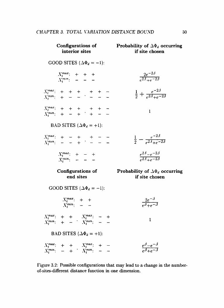
5.2 Possi Mc roiifigurat ions t hat ma\. lead to ü change in the riunilm-

of-sites-cliffcrerit clistancc function in one dimension. . . . . . .

3 . 3 The nuniber of iterations requircd for various error tolerances

in total variation distarice (indicated as the probability not

coiipled) based ori 1000 simulations. . . . . . . . . . . . . . . .

3.4 .A sirniilatecl restoration of a 33 x 32 image. (a) true image:

(b) observecl image: (c) samplc from the posterior distribution. 66

4 -4 siniulatecl restoration of a 32 x 32 image. (a) true image:

(b) obserwd image: (c) the mean of 10 independent snmples

from the posterior distribution. . . . . . . . . . . . . . . . . . 95

6.1 Relationships among probability metrics. . . . . . . . . . . . . 124

List of Tables

4.1 Convergence tinirs for the restoratiori of ir grey-scale image. . 93

6.1 hbbreviations for metrics uscd in Figure 6.1. . . . . . . . . . . 125

xiii

Chapter 1

Introduction

1.1 Introduction to the Problem and Sum-

mary of Thesis

Llarkov diain Alonte Carlo (hlChIC) algorithms were first used in stiitistical

physics and later in the stat ist ics coniniuriity for problems in spatial statis-

tics. inr liicling image processing. Sec Besag, Green. Higclon and 1 lengersen

(1995) for some histop. The. are now widely used, particularly in Bayesian

analysis. for esploring cornplicated probability distributions. See. for exam-

ple. Gelfand and Smith (1990), Besag and Green (1993). Smith and Roberts

(l993). Besag et al. (l993). and Gilks, Richardson and Spiegelhalter (1996).

An importarit issue in the implementat ion of hICSIC algorithms is whetlier

they actually converge to the distribution of iriterest. and if so. how cpickly.

For a. discussion of these issues see, for example. Tierney (1994) arid Roberts

and Rosentbal (1998). Convergence diagnostics do not guarantee conver-

gmce. ancl are knoivn to iiitroduce b i s into the rcsiilts (Cowles. Roberts

iind Roseilthal 1997). 'tluch work has k e n done in establistiing t tiroretiral

rcsul ts (see Section 2.4.2) but the- exist orily for special cases iirid are of-

tri1 clifficult to apply in practice. Exact sampling algorithiris (sce Propp and

\\-ilson ( LD96). Fil1 ( 1398) and Section 2.-1.2) wliicb tcrniinatc s i t h a srniple

distributcd exactly according to the clistributiori of iriterest holcl prorilise.

part iciilarly on finite st ate spaces. and recent extensions arc allowi ng t tieir

use iti some esamples on cont inuous and tinhoiindccl st ate spaces.

In tliis tliesis ive find precise, a priori bouncls on the convergence tiriie

of SIarkov chain Monte Cürlo algorithms iised in Bayesian image restora-

tiori. Our results can also be applied to bounding the convergence tirne of

the coiipling-froni-the-past exact siimpling algorithni of Propp and Wilson

(1996). We consider convergence in both total variation distance and the

Wasserstein metric. Bot h of t hese metrics have a coupling characterisation,

w hich is used in the developrnent of our results. Our total variation distance

resiilt is restricted to discrete state spaces ancl iLIarkov cliains for which a

partial order exists on the state space which is preserred by the Markov

chain transitions. No such restrictions are necessari for our geiieral result

t'or cotivcrgence in t tie hsserstein metric.

111 the Bayesiim approach to image restoration we observe a clistorttd

itiiiigcj ( t h e data) anci have a statistical moclel (the likelihoocl) for how the

true image was randonily distorted to give the o b s e n ~ d image. We d s o

haw a prior distribution on possible images. The priors we use place greater

prol)iil>ility on images in which neighbouring pisels are siniilar. C E nish

to rsplore the posterior distribution for the true imap . Our goal may be

to i i s r saniples from the posterior to estimate the niem u po.~tenon' image.

or p d i i i p s to find the posterior niocle to use as our restoreci image. Our

distributions are very high-dimensiorial (the dimension being the nurnber

of pisels) ancl the normalising constants are often intractable. However.

btwwiscl of the spatial structure in the prior, they are well-suited to bIarkov

chüin Monte Carlo. See Geman and Geman (1984) and Besag (1986) for

eiirly descriptions of this approach to image restoration and Green (1996) for

a more recent discussion.

For a binary image using an Ising mode1 prior. we obtain bounds on

the convergence time of the randoni scan Gibbs sampler algorithni ttiat are

0(:V2). where 'i is the number of pixels. with a coniputatioiially simple

constant of proportionality. These bounds hold for small values of the prior

paranieter. Convergence is meiisored iri to tel variation distiince aiid at each

iteration only one randonil'; chosen pixel is ~ipdated. C\R provicle rcstilts for

t tic cast. wheri the distribution of interest is the prior. which is of irit~rcbst in its

own right iti statistical physics. aricl for two randorn distortioii mechanisrns:

aclclitivc normal noise. ancl the inrorrcct observation of each pisel witli a fised

probability. These results arc prrscntccl in Chaptcr 3. While it is known in

t tic statistical pliysics literatore that the convergence tirne of these algorit hrns

is O(.V log Y) for appropriate values of the parameters which incliidc those

for atiich Our results Iiold. the proportioiiality constarit for t hose results is

intractable (see. for example, 'vlartinelli (lggi)). In Chapter -4 we develop

precise O(.V log .V) bounds for the convergence time of these algorithms by

another rnethod.

In Chapter 4 Ive introduce a niethod for bounding the tinie neccssan;

to achieve convergence in the Wasserstein metric. We apply this method

to the restoration of a ge-scale iniage where each pixel takes on a value

in the interval [O. 11 and nre achieve computationally simple results that are

O ( X log X ) . Again we use the randoni scan Gibbs sampler. Siniulations

show that Our results are reasonably tight. Moreover, because a simple bound

e'sists on total variation distance in terms of the \iVasserstein metric on finite

state spaces. we are able to use the method developed in this chapter to

iniprove the results of Chapter 3.

The met hods descri bec1 above reqiiire the analytic calculat ion of parani-

cters of the h r k o v chains relating the distancc bctween two coupled re-

alisations of the chain ta the distance at the previous iteration. In most

applications. these constarits will be ciifficult or impossible to calçiilate. In

Chapter 5 we clernonstratc~ how auxiliary simulations can be used to get

reasonable approxiriiations for these parameters. For coniparison. ive use

auxiliary sirnidation to approxitnatc the grey-scale result in Chapter 4. This

approach is seen as a coniproniise betweeii the guaraiitees of Our theoretical

results, and the uncertainty associated with the use of convergence diagnos-

tics,

Total variation distance is the usual nietric used to qiiantify convergence

of W M C algorithms to their stationary distributions. However, its coupling

characterisation requires exact coupling, which may not be practical on con-

tinuoiis state spaces. or may require an algorithm that is more difficult to

theoretically analyse. This was oiir motivation for using the Wuserstein

nietric which only requires coupling to within a tolerance c: we wanted to

estencl Our results of Chapter 3 to an image of continuous gre-scale pixels.

ï he literat ure on pro ba bility metrics is vast, and clitfererit applications use

different metrics to suit the necessary calculatioiis. In researching the choice

uf iiietric. we found that no rotirise. straightfonvard siininiary of metrics and

tlirir relationships exists. Cliapter û is an atteinpt to fil1 this gap. We tiave

selrcted nirie popular cboices of tlistaiice between probability itieasiires. wtiich

are popiilür either because of tlieir theorcticxl propertics. or their practical

iisrs. CVe have srirnrnarisecl al1 known relationships between them. Proofs

are given for relationships ancl extensions to known relationships that are

not known to exist elscwhere. It is hoped that the niaterial in this chapter

\ d l be useful to practitioners consiclering the choice of nietric. especially if

interest lies in usirig one rnetric to get results in anothcr.

Chapter 7 sumniarises sonie ideas For future work ancl extensions of the

i d e s in this thesis.

In Chapter 2 we outline the construction of MCMC algorithms and some

relevant XIarkov chain theor-

Chapter 2

Markov Chain Monte Car10

Algorit hms

2.1 Introduction

Suppose ae have a probability distrihutioti r( .) on r state space X. Iri appli-

cations in aliich MC'VIC is necessary, n(-) is typically very higli-dimensional

or so coniplicated t hat standard t ecliiiiqucs such as nurnerical ici tegrat-iw

with respect to n(.) or direct sampling from T ( - ) are not suitable. In rnany

applications in Bayesian statist ics and in stat istical mechanics. the normal-

ising constant for *(-) can not be computed.

SIChIC proceeds by coiistructing a discrete-time hIarkov chah {&} such

t hat a(-) is the unique limiting distribution. Let P(r . .) represent the tran-

sition kernel for this hlarkov chain, i.e. for each x E X and -4 C X , P ( x . -4)

represents the probability of jumping from x to soniewhere in A. Pi(x, -4)

represents the probability that the Slarkov chah iri statt. r is somewhere in

-4 after t itcrations. CVe need to construct this transition kerne1 such that

P t ( x . A) 3 K ( - 4 ) as t -t a, for al1 initial states x.

2.2 Some Markov Chain Theory

Ttic follocving hlarkov chain results can be found in Billingsley (1986) or

Feller (L9G8) for discrete state spaces, and bleyn and Tweedie (1993) for

general state spaces. See Tierney (1994) and Smith aricl Roberts (1993) for

summaries in the particular context of SIarkov chah '\'Ionte Carlo.

The distribution R is stationary with respect to a transition kernel P if

for A' discrete:

r(r)P(z , y) = ~ ( y ) for al1 y E X m 5 Y

or for A' continuous:

In practice. it is often easier to verify the following condition, knorvn as

reuerszbilzty or detailed bulance:

If rcvcrsibility holds For a distribution r with respect to P tlien it is easily

seeti that A is statioriary for P by integrating both sicks with respect to r.

A Slarkov chairi on a tliscrete state space is imeducible if it is possible to

cvrtitiidly gct frorii evcry stiite to every other. i.c. for wrry pair of states

+. g E X there exists a positive integer k such that P k ( r . u ) > O. It is

upwiodic if gcd{P > O : P ~ X . r) > O} = 1 for every r E .Y. -4 llarkov cliain

on a cliscrete stüte space with stationary distribution n mil1 have a as its

unique lirniting distribution if it is both irreducible and aperiodic (see. for

example. Billingsley (1986. Ttieorem 8.6) ).

For general state spaces. we have the following analogues of irreducibility

and aperioclicity (see. for example, Rosenthnl (1999)). Let T.., be the time of

the first visit to -4 for an' -4 E X, i.e.

If ( 1 : -Yt E A } is empty, set T.J = m. -1 AIarkov chain is pimeducible if

there exists a non-zero probability measure Q on X such that for any -4 5 X

with 4.4) > O. ive have P r ( q < MI& = x) > O for al1 r E X. i.e. any set

of positive @ measure has positive probobility of being hit froni any starting

point x. Such a rneasiire 4 is called an zrreducibilzty measure. It is aperiodic

if there does not esist a partition of the s ta te space X = .-Y~&~'~u.. . UX~ .

where u iridicata disjoint union. such tha t P(r . Xi+, nioci ) = 1 for a11

r E XI. Siiçh il r-yciic: partition. if it exists. is unique iip to sets of nicastire

1 O. \Vc consiclcr coiivcrgence of the Slarkov chain in total variation distance .

The total variat ioii distance between two pro bability trieasiires p . v oii a

space X is

dTi.(p. V ) = sup Ip(.-\) - v(.-!)l. ;ic.u

Total variation clistiirice ha5 the following equivdent forinulat ion

wherc h : X + R satisfies Ih(z)l 5 1. IF the state space X is countable.

For Our Blarkov chains with initial state J, transition matrix P and stationan

distribution n, WC are interested in how dose the distribution of states at tirne

'Note that sonie authors (for example, Tierney (1996)) define total variation distance

as tivice Our d u e .

t is to the stationary distribution, i.e.

Proposition 2.1 dTl- ( P t (r. .)' T(-)) is a non-increasing fvnction of t.

Proof

11 Pc(x . d g ) ~ ( 9 . -4) - / ~ j d y ) ~ ( y . -4)

h( . ) = P(-. -4) is a Functioii satisfying O 5 h 5 1 so using the formulation of

total variation distarice (2.1) gives

Rosent ha1 ( 1999) proves the following theorem. which is also available in

Mcyn and Tweerlie (1993).

Theorem 2.1 Let P ( x . d y ) be the transition probubilzties for u iIIarko,u chain

on u yeneral state q a c e X. Suppose there exists a non-zero probabilitg mea-

sure p svch that the ilfarkov chain is 4-irreducible. and also suppose that

the Marko,u chain is aperiodic and has stutiona.y distribution T . Ther. for

R- ulrnost e v e q x E X, ure have

lim d T I . ( P t ( ~ . a ) , n(.)) = 0. L - K a

To havc thc rcsult in thc 3bow thcorcrn hoici for al1 initial statcs x, WC

recluire the stronger coriclition of Harris rccurrence. .A hlarkov ctiairi is Harris

recw-rerit if there exists a non-zero nieasure o on X siich that if 4 4 ) > 0.

t heri

P ~ ( T . . \ < .XI.\; = r) = 1 For a11 r E X .

Often. the goal of Slarkov chain h n t e Carlo is tu generate saniples Froiti

T r iri order to estinlate E,[g(r)l by Et=, ~ ( 1 : ~ ) wherr L., - îr. i = 1.. . . . T .

The ergodic theorem (Sleyn and Tweedie 1993. Theorern 17.1.7) confirnis

thnt this is an asyrnptoticaliy consistent estiniator. despite the lack of inde-

penderice in thc Slarkov chain samplcs.

Theorem 2.2 1j {SI) W u Harris recurrent Mnrkov chain with transition

keemel P and s~utionanj distribution R , und (I is a real-ualued function wzth

cilniout surely.

CK4PTER P. ,II.~R~~'OVCH.~INAIO~VTEC-~RLO.-~LGORITHLLIS 13

2.3 Constructing MarkovChainswiththeRe-

quired Stationary Distribution

Iri this section, we will assume that oiir chr ibut ion of interest T lias ii cierisicy

wi t ti respect to ü clominating rneasure (usiially t lie Lebesgue niemure). We

will deriote t his derisity also by ~ r .

2.3.1 The Metropolis-Hastings Algorit hm

Ctioose ü proposal density q(glx). At each step. propose a new statc y froni

q giveri the current state r. Accept the riew state and move to it with

pro bability

or reject it aiid stay at the same state witli probability 1 - a(r. y). If

~ ( s ) cl(&) = O. set a(c. y) = 1. I t is easily seen that tliis hlarkov cfiain

is reversible with respect to n. For example iii the discrete case. if r # 9,

So T is a stationary distribution. The following results are in Tierney ( PB-!).

Consider q(ylx) as the density for a 'rlarkov chain. It is necessary for it to bc

a (o-)irreducible LIarkov chain for the resulting hletropolis-Hastings chain

also to be (+)irreducible. Harris recurrence is often achieved for hlctropolis-

Hiistirigs algorithrns because a 4larkov chain is Harris recurrent if P ( r . - ) is

absolutely continuous with respect to its stationary distribution s(.) for d l

startirig points x. or if a is an irreducibility nicasure (Tierney 1994).

The special case where q is symrrietric. i.e. q ( y ( r ) = q ( r l y ) is callecl the

. \ k t ropolis algorithni after the work by SIctropolis. Rosenbluth. Rosenbliit ti.

Tellrr and Teller (1933). It was generalisecl by Hastitigs (1970).

2.3.2 The Single-Component Metropolis-Hastings Al-

Suppose ir(-) is the joint distribut ion of r = (r l , rl. . . . . rLv). Sonietinies

it is cornputationally simpler to update only one cornponent of x at each

iteration. Suppose at iteration t + 1 component i is being updated. The

proposal distribution is t lie univariate distribution wit h density g(y i lx i , r -, )

v e r x , = ( x . . . . x , , + . . . . x). The proposed value for component

i is acceptecl with probability

TIic rtmairiiiig coniponents are not changed at itcration t + 1.

The coniponents can be iipdateci in a systeniatic or rancioni order.

2.3.3 The Gibbs Sampler

Again suppose T(.) is the joint distributioti of (x ,. r-. . . . ..r,v). Each coni-

ponmt is iipciated according to its conditional distribution givcri the ciirrerit

~ali ic of racli of the other cotiipoiierits

Thtw clistrit>iitions are cülled the full conditionals. The comporients can

eit hm br upclated in rendoni order or in a systeiriatic order. The random scan

versiori is easily shown to be reversilde. While the systernatic scari version is

not revwsible. w is a stationa. distribution for the resulting 'ularkov cliain

(orie iteration comprising one sweep of the components) since it is a stationary

distribution for the update of eacli individual component.

The Gibbs sarnpler is a special case of the single-component hIetropolis

Hastings algori thm where the proposals q are the full condit ionals and the

acceptance probability is always one.

The Gibbs sarnpler was giveii its name in Geman and Geman (1984)

where it was used in Bayesian image rcstoration. Gelland ancl Sniith (1990)

estcnded its application to cotitinuous state spaces and showed how it can

be iised in Bayesian inference problerris.

2.4 Convergence Issues

2.4.1 Qualitative Convergence

.\ hlarkov c h i n is yeornetn'cully eryodic if

dTI- (Pt (2 . -). K(*)) 5 .\1 (x)$

for sorne finite .\l(r). and constant p < 1. It is unljoonly e r p d z c if for ail x

d T \ * ( P t ( ~ , * ) , T ( * ) ) 5 .\fpt.

h scat C C X is small if there exists a probability mesure # and constants

c < 1 and positive integer k such that

pk(r. * ) 1 cd(*) for al1 r E C.

.A SIarkov chain is geometrically ergodic if and only if it satisfies a geometnc

drift condition. i-e. there is a small set C aiid coristants X < 1 and b < cx:

and a x-almost everywhere finite function : X -+ [I, ml such that

/ \-(y) P ( L dg) 5 A \ -(=) + bl&)

(see Xey il aiid T werdie (1993. Cliapter Id)) .

-4s ml1 as being likely tu coiivcrge reasonably cluickly in practice. geoniet-

rically ergodic chains are iiseful becausc a Central Limit Theorem exists for

avcrüges of fiinctions of thcir output (see Chan and Geyer in the tliscussiori

tao Tierney (1994)).

If the cntire state spacr is srnall, then the Slarkov chain is iiniforinly

ergotlic. This doesn't often occiir iri statistical riiodcls with unboiiiidcci statc

spaces. but is necessa- Tor the coupliiig-from-the-past algorithm descrihcd

in the next section to work (Foss and Twedie 1998).

2.4.2 Quantitative Convergence

CVe now turn our interest to the criticel question of how many iteratioris of

the Xlarkov chah are necessa- in order to be able to consider the output to

be a sample from the stationary distribution. There exist three approaches

to answeriiig this question: convergence diagnostics, theoretical results. and

esact simulation,

Convergence Diagnostics

Convergence diagnostics are nietliods of monitoring the convergence of the

algorithni while it is running by considering statistical functions of the output

of ii sirigle chain or of multiple runs of the same chain. Tliere exist rnariy such

proccdiires (see Cowles and Carlin (1996) and Brooks and Roberts (1997) For

reviews) but none arc cornpletely sat.isfactory. Al1 convergence diagnostics

arcB kiiown to sonietimes preniatiirely claim convergence (Cowles arid Carlin

199G) and cati introduce bim into the resiilts (Cowles et al. L997. Roberts

and Rosent ha1 19%).

Theoret ical Results

Thrrc has been niuch work on tieveloping rigorous. a priori. quantitative

hoiirids on the convergence tinie (For example. Sinclair and .Jerruni (1989).

Diacoriis and Stroock (1991). Frieze. Kannan and Polson ( 1994): Ingras-

sia ( l99-L), bIeyn and Tweedie (lW3), Rosenthal (l995b). hlengerson and

Tweedie (1996): Polson (1996). and Frigessi, blartinelli and S tander (1997) ).

Howrver, these resiilts exist for specific problems and may not be general-

isable. they require extensive and complicated calculations. and the upper

bounds they provide on the convergence time are often overly conservative.

bloreover, for some of these results. the order of convergence is known. but

the proportionality constant is not available.

Developing theoretically justifiable convergence rates for problems in Bayesian

irriage restoratioci is the subject of most of this thesis.

Exact Sampling

Rcrently. thc dcvelopment of algorit hrns t hat produce sain ples ciistributed

exactly arcorcling to the dist ribiit ion of interest (Propp aiid Wilson 1996. Fil1

1998) have gcnernted a great deal of interest. Because we will later describe

tiow oiir results iri Chapters 3 ürid 4 ran tx used to bouiid the ruriniiig tinie of

the coiiplirig-frorn- the-past (CFTP) algorit hm of Propp and Wilson (1996).

we give s t~rief description of the algorithm here.

CFTP is a methocl of organising a lIarkov chah simulation so thiit it

delivers exactly a sample from the distribution of interest. The nuniber

of steps necessary is random arid deterniined by the algorithm as it runs.

Suppose we could start the Markor chah in every state a t time -oc. Then

if al1 realisations of the chain starting at time -a? have the sarrie state at

tinie 0. we have lost al1 dependence on the initial state and this common

state rnust be a sample froni K. In practice. if t here e?cists an initial tirne -T

such that for al1 initial States -KT, -Yo is the same. then .Yo - ir. And we

(lori't need to fiiid T exactly since coalescence occiirs froni al1 initial tirnes

less than -T if it occiirs from -T. Propp and Wilson s~iggest the doubling

strategy of starting üt tirne -2, and if coalescence is not achieved. next start

itt tirne -4 atici ttien -8. etc. This is valid as long as the uniforni raiidorn

iiiirriber used ilt each time point remains constant.

If the state space is large or irifiriite it rnay tw ciifficiilt or inipossible to

kwp track of Ilarkov chuins startecl in each possible stiitc. This difficiilty

is ovcrcoriic for monotoric LIarkov chains sucti ii.; those considerecl in the

iipplirations iri ttiis thesis. t r i our esaniples, there rxists a partial ordering

on the state space witb iiniquc maximal and mininial rlemcnts. .\Ioreover,

t h . htarkov chain transitions presenfe this order. Thus it is only neccssary

to iichieve coalescence of the chains startecl in these rriasirrial and minimal

stiites. as t liis guarantees coalescence from d i initial statcs.

More formally. suppose we have a sequence of independerit Uniform(0. l]

randorn variables. <,. i = -ca . . . x and we cari find a deterministic function

/ : X x [ O . 11 + X such that the value of the Markov chain st time t + l is

clctermined as

* b + l = f (-&,&).

If f is monotone in the first variable, chains begun in higher starting points

will stay übove chains begun iri lower starting points. i t follows that

P(1.1:. 30)) 5 P(& [ z . x))

for al1 : E .Y. Suppose S;'ax and -Y;"'" are the states at tinie t for the diains

st artrd in t lie niaxirnal and iiiinirnal states. respectiwly. C pclatirig according

to ('1.2) ensiires that a chain. K:. started in any other initial state will be

san(lwiclicc1 hetween the niaxirnal and minimal chains. i.c.

Thus coalcs~eiice of chai~is started in the mi~~ in i a i arirl rnininial states is

sufficirnt for coalesccricc of chairis started in al1 possible points.

Tlie esterision of CFTP to infi nite discrete state spaces ancl cont inuous

state spaces in special cases has been considcred and appliecl hy. for example,

Foss aiitl Tweedie (1998). Green and hIurdoch (1998), Xlurdoch and Green

(1998). Corcoran ancl Tweedie (1998), Noller (1999). XIiirdoch (lggg), Moller

and ?licholls (1999), and Giiglielmi, Holmes and CValker (1999).

2.5 The Coupling Method

The coupling rndiod exploits the coristruction of a joint clistribution with

given marginals to prove things about the marginal distribiitioris. For a

detailcd discussion of ttie coupling method see Lindvall (1992). In our ex-

miples. we consicler couplecl hliirkov chains on ttie state space X x X. The

niarginal clistribii tions sri? the distributions of 1Iarkov diains wit h differ-

erit initial statrs. biit hotli Following the transitions OF tlie original XIarkov

chüin. Our coiipled chairis will not procced indepericlcntly: we mil1 use tlic

same iiniform r d o r t i iiunibcr to deterniine their transitions at each step.

This clepen<ieriw is neccssary For our construction of Alarkor cliaiiis which

are nioriotonc.

Lintlvall (1992) provides man- applications of the couphg method. in-

cluding its application to provicling estirriates of convergence in total variation

distarice for .lIarkov cliains. Sorne other applications of coupling that are rel-

evant to Slarkov chain Slorite Carlo include the proof in Rosenthal (1999) of

Theorem 2.1, and the convergence results of, for example, Rosenthal (1995b)

and Luby. Rariclall and Sinclair (1995).

Chapter 3

Total Variation Distance Bound

for a Binary Image

3.1 Introduction

In tliis chapter. uve show Iiow coupling niethodology can be used to give

precise, a priori bouncls on the convergence time in total variation distance

of hlarkov chein Monte Carlo algorithms. Our results hold for monotone

Xlarkov chains, for wtiich a partial order exists on the state space which is

preserved by the Markov chain transitions. In partiçular. we develop con-

vergence time bounds for a simplified problem in Bayesian image restoration

wliicti involves sampling from a Gibbs distribution using the Gibbs sampler.

The case of image synt hesis, where there is no observeci data, is equivalent

to what is referred to in the mathematical physics literatiire as Glauber dy-

niiniics for the stochastic k ing model.

LVe use coupling and martingale techniques to obtairi precise upper bounds

oii the convergence tinic in total variation distance for the random scan ver-

sion of the Gibbs sampler. where each iteration involves the update of orily

one randomly chosen pixel. For appropriate valiies of the prior parameter.

oiir hoiincls are an easily coniputnble constant tinics .V2. where .V is the niim-

Iivr of pisels. While WC believe t tiat sirnilar argunierits will lead to a sirriilar

hoiiiid on t lie convergerice time for the systematic sciiri algorit hm. tlie fact

tliat the values of neighboiiring pix~ls may change at each iteration milkes

aiialysis of the systematic scan algorit tini more clifficult . The general met hod-

ology oiitlined in Section 3.3.1 can be appliecl to any monotone Markov chain

Monte Carlo algorithm. In Chapter 4 we show tiow tlie calculations of this

cliapter can be applied to achieve precisc bounds that are O(.V log X ) .

In the mathematical physics literature, it is well known that the conver-

gence rate for the stochastic Ising mode1 is O(Y log N ) for appropriate values

of the parameters which include those for which our results hold. (See. for

exarnple. Frigessi et ai. (1997).) However the constant of proportionality is

not known.

Our results are presented as follows. The niodel and Gibbs sampler algo-

rithni are descri bed in Section Y .S. The coiipliiig niethodology used to derive

oiir boiirids is cIt.scribed in Section 3.3.1. Ttii. iipplication of t hese boiiricis

to tlic rurining tirrie of the coupiing-frotii-tlie-past algorit hm of Propp and

\\'ilson (1996) is cliscussed in Section 3.6. R~siilts for sanipling froni the

king rnotlel witliout data aiid from the posterior distribution with data are

presentd in Sections 3.4 and 3.5 respectively

3.2 Image Restoration using the Gibbs Sam-

pler

3.2.1 The Mode1

We corisicler the Bayesian restorütion of images where the prior consists of

a probability mode1 for the true image and the posterior is formed from

the prior conclitional on the data, which in our cases are the values of the

observed image. These observed data are obtainecl From the true image

through a knowi random distortion process. See Gemaii and Geman (1984)

and Besag (1986) for early descriptions of this approach to image restorat ion

and Green's article in Gilks et al. (1996) for a more recent discussion. The

raiiduiii scaii Gibbs saiilpler is used tu produce saiiiples froni the posterior

distribution. We also consider the lise of the Gibbs sanipler for simulation of

the prior distributiori since this is of interest on its own.

Oiir mode1 of the image is a 4Iarkov randoni field of pixels taking values

iri { + 1. - 1 1 . wit b t lie value of each pixel affectecl by its nearest neighbours in

;in at tract i w nianrier. Equivaleritly it is niodelld by tlie Gibbs distribution

1 ~ ( x ) = - esp (-L(r)} (3.1) z

ahcre r = ( x l . . . . . rs) is a configuration of the colours a t the .V pisels.

the cnergy fiinction C: refiects the neighbourliood structure ivitliin which

cotifigiirat ions with pixels having like neighboiirs are favoured. and Z is the

normalising constant. ralled the partition function in mat hematical physics.

The particular prior probability tnodel we place on the configuration is the

king niodel for wtiich

where the sum is taken over pairs of sites (i, j) which are nearest neighboiirs.

and LI is a positive paranicter. For a discussion of the physical significance

of the Ising motlel, see Cipra (1987). Conditioning on the value of observed

data results in a posterior distribution that is equivalent to a Gibbs distribu-

tion with the presence of an external field. With the Ising moclel prior. the

posterior ciistrilutiori of L giveri tiie data. y, is of the forni

t tie normalising constant which is a function of the data. and the

funrt ion / changes \vit ti the randoni distortion mechanisrn.

O u r clata arc an observed distortiori of the true iniuge. C \ é corisider tmo

distortion r~iecliariisms. In Section 3.3.1 ive çonsidcr y to be obtainrd froni t lie

triir image by switching. with a constant probübility the sign of each pisel

anci in Section 3 . 5 2 me consider tlie case where iriclependent normal noise is

arlded to the wlue of eaçh pixel. Exarnples of tlie forin of the function f in

(3.3) ;ire available in Eqiiations (3.21) and (3.24).

E w n for the simple models stuclied tiere, examining both the prior and

posterior distri butions by calculating the probability of each configuration is

impracticd becaiise of the large configuration space. For example. a grid of

64 x 64 pixels has 2''096 configurations.

The Gibbs sampler is used to produce a sample from the distribution of

interest. Pixels are updated according to t heir conditional distribution given

the value of al1 of the other p~uels. At eacli iteration one randomly chosen

pixel is updated. The algorithni is outlined in Section 3.2.2.

3.2.2 The Algorithm

Our goal iri the Bayesian image restorutiori process is to prodiice saniples

froni t be posterior distribution of the in iag~. These sarnples can he usecl to

explore the postcvior distribution. with goals such as finding its modc(s). or

calculating ~sprrtatioris. We use the single site random scan Gibbs sanipler

to obtain tlicsc rirritlorii samples. Wc also consider the application of the

algoritlm to ttir riut? without data: we ;ire then sampling frorri thc king

niodel prior dist ribiit ion.

For Our prol~ltvii. the Full conditional probabilities are easy to calciilatc

and to sarnple honi. They do not recluire the calculation of the normalisirig

constant and dep~rid orily on the current values of the nerrest neigtibours.

In the case of senipling from the posterior conditional on the data. the full

conditional for earh pixel depends on the value of the obse~ecl image at

that site. and no other observed pixels. For the case of no data where the

distribution of iriterest is the king mode1 (3.1) and (U), the full conditionals

are

where the suni is taken over pixels j that are neighbours of pixel i. For the

case with data, the full coriditionals are

where the fuiictiori / conies from the random distortion mechanisni that

creates the obscrved image.

The iterations continue until the currerit corifiguration can bc consiclertd

to be a saniple Froni the posterior distribution. iridependent of the initial

configurat iori. NP are concerned wit h the nuniber of iterations required.

The Markov chain whose state space is the space of al1 possible config-

urations and whose trarisition probabilities are $ times the full conditiorial

probabiiity. with transitions only possible between configurations which clif-

Fer üt only one site. is an irreducible. aperiodic SIarkov chah with stütionary

distribution n.

3.3 Bounding the Convergence Time of the

Algorithm

Convergence is measured by the total variation distance (tvdj, which is

the tisual nietric chosen to assess corivergence of .\lCBIC algorithms. For

;L 1I;irkov chain with probability trarisition matrix P. stationary distribu-

tion rr. countable state spacc X. and initial configuration xo E X. the total

variation distance at thne t is

aliere Pt (2'. L ) is t tie probability that t lie Markov chain with initial state ro

is iri statc r at iteratiori t. and -4 is any set. As shotvn in Proposition 2.1.

tvcl,~(t) is non-increasing in t. The convergence tinie of the lhrkov chain

iised by the Gibbs sampler is defined as

r ( r ) = maumin{t : trd,~(t') 5 c for al1 t' 2 t ) x"

(3.8)

where c is a pre-specified error tolerance. chosen at the user's discretion.

Propp aricl Wilson (1998) use the arbitrary value l /e as the value of e which

gives t beir tnixing time

distance (3.6) leads to

threshold. The first definition of the total variation

perhaps the clearest interpretation of the choice of

: for every possible set .-I in the state space. convergence to within c in

total variation distance guarantees that the difference between the probability

that oiir SIarkov chain is in -4 aiitl thc probability of .-l for the stationary

distrit)iitioti is at niost f . Tlie relationsliip between the value of c and the

nimber of itrrations required is furtlier esplored through sirnulatiori of the

stocliast ic: Isirig rnociel in Section 3.4.

Rrquiriiig t hat the total variation distarice is less than c givcs an imniecli-

ate toleranrc on the error due to la& of coiiwrgerice iri the estimation of t lie

espectation of hountled functions. This is because of the followirig equivalerit

forniulatiori of tvd

1 v i t = - nias J y h pt(r0.dx) - Jr h * ( d x ) (

2 ( I r ( < 1

where thc niauimum is taken over functions h : X + R satisfying slip, Ih(r)J 5

1.

WC are concerned with the number of iterations required to achieve con-

vergerice for a given algorithm, and riot rvith other important issues such as

the variarice of estimates of erpectations (see, for example. Green and Han

(199)) ?VP recommend that our results be used to determine the number

of iterations required to achieve stationarity. The siniulation of the Markov

chain can then be çontinued beyond this and ttese adclitional values used for

piirposes such ÿs estimating cxpectations.

Our results are ail application of coupled Markov chains. The coupling

ttwt liodology is presentecl iri Section 3.3.1. In Section 3.6 we discuss how tliese

resiilts cati bc üpplied to exact sarriplirig algorithms involving coupling-froni-

the-put. Other metliods for achieving a bound on (3.8) are disciissed in

Section :3.3.2.

3.3.1 Using Coupling to Bound the Convergence Time

O i i ~ triethocl of bouridirig the convergence time of a Slarkov c h a h r ( r ) .

is ttiroiigti monitoring two couplecl Markov chains. Suppose .Y: and .Y?

;ire t ao Markov chains on the sanie state space, with the sanie trarisition

prohabilit ies. and wit h initial values x1 and r' respect ively. At each iteration.

the si-triic iiniform randoni nuniber is used to determine the transition for both

chains. They are said to be couplcd at time T''-~' if

Our hoiind on ~ ( c ) will be iri ternis of the maximum mean coupling tirne

ivhi.r~ t tir niaximiim is takm owr iill pnssihk initial s t n t ~ s .rl for .\;' and .c2

fo r .Y) .

.-\s show in Aldous ( l983). t lie following relat ioriship exists between t tie

r r i t w i cociplirig time and the convergence time:

TIw nirthod iised herc wis inspired by that of Luby et al. (1995) whose

llarkov rhiris were lattice rocitings in orcler to genwate a raiidorri tiling

of ii plariar latticc structure iri striclying the conihinatorics of tiling two-

diriicmionül lat tices. They use coiipling to get bounds on the convergence

tiriie of tlieir Markov ciiains that are polynomial in the size of the lattice.

For oiir niodel for binary images. a partial ordering exists on the set of

al1 (wrifigiirations. One configuration is greater tlian another if each pixel of

the larger configuration is greater than or equal to the corresponding pixel

of the smaller configuration. CVe set the initial configurations of the two

chains to be al1 +1 and al1 - 1. CVe label these configurations xma' and sr*'"

respectively. Our process will preserve this order: the chain that starts in the

mauinial state will alwqs be greater ttian or equal to the chain that starts

iii the niininial state. This is because at each iteration our algoritlm will

use the same random niimber to cleterniine the transition for both chains,

and the updare function is a deterministic fiinction of this random number.

arid a monotone function of the ciment state. In particiilar. suppose at

iteration t site i has been choseii for iipdating and & is the L'niforni[O.l]

rariclom riurnber to bc used iised for updating at t hüt iteration. If the value

of the full coiiditiorials (Eqiiatioris (3.4) or (3.5)) evaluated at r, = +1 are

less thaii or equal to me set t h e value of pisel i at tinie t + 1 as +l. Ttic

fil11 conciitionals place greater probability on configurations in which pisels

are like ttieir rieighboiirs. arid the chain started in the niwimal state will

have at least as many neighbours of pixel i ttiat are + L as the chain started

in the rniriitnal state. Thiis the value of pixel i in the chain startecl in the

maximal state will always be greater tlian or equal to its value in the cliairi

started in the minimal state.

As argiieti in Propp and Wilson (1996) for monotone hIarkov chains sucli

as this. it suffices to consider the case where the initial configurations are

the estrerne states. Chains started in any other initial states rl. x2 (xm'" < = l < x2 < =mal - - ) must couple in a tinie less than or equal to the coupling

time for xml" and xma.r for the same set of random numbers determining the

t rarisitions.

Let 9(t) be a fiinction tliat assigns a positive integer to the difference

hetweeii the configurations at tinie t ot' the Markov ctiains started in the

niiiuinial and minimal statcs. O should be defined sucli thût (P(0) is .V. the

riiiniber of sites, and O 5 @ ( t ) 5 .V for al1 t . Two chains will have coupled at

tinie t if @ ( t ) = O. Once cocipled. the? will reniain so. Define the coupling

t irrie

T ~ ~ ' ' ~ Y1in = i n f i t : @ ( t ) = O}.

Thcii

Let M ( t ) = 3>(t + 1) - 9(t) denote the change in the value of 9 after

one iteration of the randorri scan Gibbs sainpler. Suppose a region of the

parameter spacc for ,i caii be found sucli that E { A @ ( t ) IS:, Sf} < O for al1

t For nhich S: # Sf. say E { h P ( t ) 1-Y:. -Y:} 5 - a d where - 1 < - a d < 0.

Tlien for these values of 3. as stiown in the proof to Theorem 3.1. the quantity

E ( T ~ ' * ~ ' ) can be bouiitled above by .Va;'.

Theorem 3.1 Suppose there exist Iwo coupled realzsations. -Y:, .\II of a

Markou chain where Si = xi and -Y: = 2%. And suppose a constant a > O

cun be Jound such that E{M(t)lS/. S:} < -a j o r ail t for whirh S: #

urher-e M ( t ) is the change in distonce between the two iCfarko+u chains from

iteratiori t to t + 1 and the distance between the initiul dates is @ ( O ) = N.

Then t he following bovnd ensts on the rneun coapling time (3.9)

Proof Define the stochastic process Zt = ( D ( t ) + ut . 2, is a superniartingale

LI^ tu tirne T ~ ' ."' sirice

T~'.'' is a stopping timc. Since Zt is iionnegative we can apply the Optional

Stopping Theorem (see. for exaniple. Durrett (1996. Tliearmi 7.6. p. 274))

giving

we have

CHAPTER 3. TOTAL CI-1RIa4TION DIST'ANCE BOCWD 37

In our examples. a is of the form y wvhere? as will be seen. / ( 8 ) is

straightforward to cornpute, as is the range of possible values of J which

guararitees that the distance function is decreasing on average. Conibiniiig

(3.13) mith (3.11) gives the forni of oiir results

\Ve hiive introducecl the subsçript d to niüke csplicit r's cleprridencc on the

u1uc of t hc nioclel parameter.

3.3.2 Other Convergence Results for this and Related

Models

In rriatlieriiaticril pliysics, tlic case ivithout data is kriown as the stochastic

Ising niodel with Glauber dynarnics and it is wvell-known that its convergence

rate. asyrnptotically in Y, is O(.V 1og.V). In diniensions higher than one, tliis

result holcls for d u e s of 3 below a critical value at which a phiise transition

occurs. Madras and Piccioni (1999) use Dobrushin's criterion to bound the

spectral gap of the Markov chain transition rnatrix. and show that for sniall

valaes of 3 the chah converges at a different rate tlian for larger values of

i' for which they show it is slowly mixing. For the Ising mode1 with an

esternal field. the convergence rate is known to be O(.Vlog N) for al1 3 in

two diniensions, ancl for srnall enough ,8 ancl large enough external field in

higtier dimensions. (Sec. for example, Mart inelli ( 1997). ) These reçu1 ts use

rile log Soboiev incqiialicy and it may be impossible to calculate a prrcist.

upper bound using ttiis niethod. so these rcsults are difficult to apply in

practict~. Wiile oiir rrsiilts are 0(.V2). Ive are able to givc the proportionality

cxmstant. Frigessi et al. ( 1997) prcsent the O(.V log 'i) results in the contest

of Bayesian image restoration. In Chapter 4 wve desc-ril)(~ Iiow the cülculatioris

of this chapter can be usctl to get a bound tliat is O('; log Y).

Tlir. total wriatioii clistance can also be botinclecl above hy a simple fiinc-

tion of the cigenvalue of the Markov chairi transit ion niatrix which is seconcl

iiirgest in absolute value. Poincaré and Cheeger ineqiiülities can be used to

get simple bounds on this eigenvalue in ternis of a set of canonical paths

on a graph associated with the hlarkov chain. The vertices of the graph

are the states of the Slarkov chain and an edge set is ctiosen between states

such tfiat an edge esists bt.twveen states x i ancl r' only if there is a positive

probability of nioving froni state ri to x2 in one iteration. See, for example.

Diaconis and Stroock (1991) and Sinclair (l992). While t his approach seems

promising in providing precise bounds, for Our image restoration problem Ire

were only able to find canotiical paths that gave convergence O(esV), even for

the orle-diniensional nioclei.

Using a piitti boiincls approach. Jerrum and Sinclair (1993) develop a

3Iarkov chain aigorit hm for estimating the partition fiinction of the Ising

rtiodel t hat t liey show is polyrioriiial t ime.

For the case with no data. corresponding to the stochastic Isirig niocle1

witti no esterrial field. our results apply for small valiics of J iri clinien-

sions higher tlian one. corresponditig to large teniperatiirc wheri the niodel

is consicirrecl in t tierriiodynaniic terms. Frigessi. di S tchno. H wang arici

Sheu (1993) consiclcr the qiiestioii of whicti hIarkov chiiiri Nonte Carlo algo-

rithm provid~s Fastest convergence for this probleni. coniparing theni via their

eigenvalues. Tliey show that. for high temperature. the single-si te hletropo-

lis algorithm gives the slocwst convergence of any rancioni scan updating

dynaniic. \C'hile the Gibbs sampler is better. they also show that conver-

gencr c m be improved by consiclering dynamics which include the current

value of the site being upclated.

CHAPTER 3. TOTAL C:4RIRI-ITTON DIST-WCE BOUND 40

3.4 The Case of N o Data: the Stochastic Ising

Wt! twill first apply o i i r resiil t to the case wliere we have iio ubserved image,

so ne are sarripliiig frorn otir prior distribution. the king mode1 withoiit a

external fielcl.

3.4.1 One Dimension

WC begiii bu c-oiisicirririg the one-dimensiorial case. with each interior sittt

equally influencecl tiy its two nearest neighboiirs. So the prior density is

and the full concli t ionals (3.4) for interior sites are

~ F C (xi lx- )

and for end sites

~ T ~ ~ ( L ~ ~ X - , ) = (i, j) = (1,2) or (i, j) = (n, n - 1). ~ s P { . ~ x , } + e?tp(-3xj}'

The Left-to-Right Sweep Distance Function

Recall that our bourid on the convergence tirne requires a bound on the

mean tirne to couple for Xfarkov chains startecl in the maximal ststc. where

each pisel is +l. ancl the mininial state. whert? cwli pixel is - 1. Define the

distance fiinctio~i bctwecn the current two states of these hlarkov chains to

de f be @, = .V - r where .V is the total numbcr of piscls and c is the niinihrr

OF sites at the right erid that have coupled. For exaniple. at some time t.

suppose t tie configurations of the hlarkov cliaiiis startecl in the maxinial aiid

tnirtinial states arc!

S:""': + + . . . + - + + ~;""': + - . . . - + +

tlirri <P,(t) = .Y - 3. Note that @ , ( O ) = .V and @,(T) = O. We cal1 this dis-

tance furiction the "Swecp Distarice Furict ion" . The following iipper bound

on the convergence time esists for sarnpling froni the one-dimensional Ising

Theorem 3.2 For surnplzng via the ra~idom scan Gibbs sarnpler from the

one-dimerisional Ising mode1 with !V sites giuen by (3. I d ) , the convergence

time (3.8) can be bounded above by

for d l uahes of the lsz7zg model prameter ul, where c is the specified tolerance

for convergence in total variation distorrce.

Proof Consider all possible configurations of a site and its neighbours for

which a change in QS may occur. Sirice we are considering the random scan

Gibbs sanlpler. one pixel is updatecl at each iteration. At each step in the

algoritlini. @ , will change by + L if the (.V - c + site changes and decrease

by 1 or more if the (.V - c)lh site changcs. We call sites which can contribute

to an increase in 9, %ad" sites, and sites which can contribute to a decrease

in 9, "good" sites. Updating a good site may result in a change in c of more

than onr i f sites to the left of the site b ~ i n g updatecl have already coupled.

However. we will create our bound by consicleririg worst case scenarios, so tvr

will considcr good updates which only decrease cDS by I. Note that. because

sitc>s to the right of the (N - c + I ) ' ~ site have the same neighbours in both

configurations. they will change in the same manner, so they cannot affect

the value of tile clistance function. If a site to the left of the (.V - c ) ~ ~ site is

chosen for updating, the value of the distance function cannot change.

The configurations of three interior sites illustrated in Figure 3.1 will

possibly result in a change to a,. The site being updated is to the left of the

boundary for good sites (the (N - c)'~ site) and to the right of the boundary

for bac1 sites (the (A' - c + l ) t h site). The top row indicates the current

configuration of .Y;""': the chain stûrted in the maximal configuration. and

t h e bottoiii con inclicates the current configuration of S;R'". the chair1 startecl

in t fie rniriinial con figuration. The uptlatr pro babilities are calculated froni

(3.15). A site is upclated to +1 if the iiniforrri randorn number iisecl at the

currerit itrratioti for updat ing is Iess ttiiui or tqual to the value of (3.13)

wtien r, = + 1. and is otlicrwise updatecl to - L. Rccall that both coupled

chairis arct iipdated with the same uniforiri randorri riurriber. As an oxariiple.

suppose tlic site to the left of the boiitid;iry iri the first configuration shown

has heeti selected for updating. Theri

Pr (A@, occiirriiig)

.Y;""': + + + configuration becomes or

.Y,"'": - + + + - + ) - - +

wtiere the minimums are over the probiihilities of Sr: and .Y;" respectively

being upclated as shown given their configurations at iteration t .

If the boundary is at the end. the end site is a good site and there are

no bad sites. This site couples with probability 1 if its neiglibouring pixel is

the same in both configurations, and with probability 2e-$/ (eu + e-') if its

Configuration

GOOD SITES (A@, = -1):

GOOD SITES (A@, < -1):

BAD SITES (la, = +I ) :

Probability of 16, occurring if site chosen

Figure 3.1: Possible configurations that may lead to a change in the sweep clistarice furiction in one dimension.

neighbouring pixels differ and the espected change in the distance is at most

If the bouiiclarv is in the interior. we obtain a bound on the expected change

iri the dist a1ic.e fiirict ion as follows.

In order to obtain an upper bountl on E[&P,] that holtls for ail corifig-

uraticins. wr assiinie that the site to the left of the boundary is a griocl site

with tlie snialltst probability of ctianging 9, and that results ii i a cliang of

@, of oiily 1. At each iteratiori. the site to be uptlated is ctiosen uriifornily

froiii t hr ii pisels. Thus

for al1 t where S;""' # Slin

< O for al1 !1.

2) -2.3 Applying Tiieorem 3.1 and Equatioti (3.12) with a = +e2d+e-+ the meari

coupling time can be bounded above by

where T hüs been defined in (3.10). and appiying (3.11) gives the result. .

For exaniple, if t= = 0.01 and ,3 = 0.5. r < 128iV2. Using a value such as

d = 1.5 gives more influence to t lie smoothing inherent in the prior distribu-

tion and gives the convergence bound T 5 6162.V'.

Xote that by considering the distance function as the total riurribt*r of

sites less the number of sites couplecl at 60th ends. the mean coiipling tirne

can he r~duced by a factor of 2.

There is no pliase transition in the one-dimerisional Ising moclel (see. for

esartiple. Cipra (1987)). so a resiilt sucti as this that liolcls for al1 J slioiiltl

exist. Hoaever. in tiigher dimensions. convergence is known to change at the

critical value of J at wt~ich pliase transition occurs. Convergenccl is kriowri

to be slow for .j abovc this value. Our rcsiilts for higher diniensioris hold for

sniall J, below this critical value.

3.4.2 Extension to Higher Dimensions and Larger Neigh-

bourhood Systems

The Sweep Distance Function

In two anci higher diniensions. there is no simple distance function analogous

to the stveep distance function of one dimension. The immediately obvious

aiialogue. where the nuniber of sites coupled r t an endpoint is replaced by the

size of a corner that is coupled, is not appropriate since, on any future step

of the algorithin. an) of the sites dong the coupled boiindary may change.

destroying the structure. An irregular boundüry rroiind the coupiecl sites

c m çliange in niariy w-S. incliicling losirig contact with any corner or edge

sites. rnaking it very cornplm to keep track of the size of the coupled corner.

Considering a cluster of coiipled sites scems to be too compiex to be usefiil.

For a systematic scaii Gihhs siirnpler it rnay be possible to defirie a dis-

tance functioii like this. sirice at each iteration al1 pixels are iipdütecl ancl the

nurnber coupled in a corner structure can be rnaintainecl.

\\é aclclress this problerli by defining a different distance fiirtction. whicli

will lead to restrictions on the values of J.

The Nurnber-of-Sites-DiEerent Distance Function

Define the distance function ad as the ntimber of sites mhere the two chains

cliffer. Then <Dr(0) = :V ancl Od(T) = O. This distance function can be

used in any dimension. \çè cal1 (Pd the "Number-of-Sites-Different Distance

Function". A change in <Pd may now occur for any site chosen for updating,

uiiless it is in the middle of a string of at least three cotiplecl sites.

Our result is stated in terrns of n. the number of nearest neighbours that

are equally iiifluential: n is typically 2 in one dimension, either 4 or 8 in two

diniensions. etc. Our upper bound on the convergence time is still a simple

fuiiction of the mode1 parameter d times .VL whcre ,V is the total number of

sites: however it now holds only for a restricted range of .l. -4s the niirnber of

infliicntial neighbours iricreases. the range of admissible values of J decreases.

Theorem 3.3 For sampling uiu the random scan Gibbs sarnyler j'rom the

Ising rr ide l (3.1) and (3.2) in ar.6itrur-g dirnrnsiorr ,uzth .V sites wlrere each

site is influerrced by its n nearest neiyhbours. the conoergericr tirne (3.8) cctn

be houvided uboue bg

fur

iuhem 3 is the Isiirg mode1 purcnneter and c is the specified tolerance for

convergence in total vuriution distance.

In two dimensions, the cri tical value for the two-dimensional Ising moclel

where each pixel has four influential neighbours is knonn t.o be log(l+ a)/? (Liggett 1985, p. 204). When ;3 is above this value convergence is known to

be slow. Our upper bound on 3 is well below the critical value. but to our

knowledge these are the first precise bounds for any value of d.

Proof of theorem Considcr al1 possible configurations of a site aiid its n

neighboiirs in which a change in the nuniber-of-sites-different distance

function. may occiir. Sirice we are using the randorri scan Gibbs sariipler. at

eadi iteratiori Od can change by at niost 1. .A sitc wtiicti can lcad to a change

iii 'Pd of -1 is considerecl a *'goood" site iiiid + L a "baclt site.

For case of prescntation. the possible coi~figiirations are illiistrated in Fig-

urt3 3.2 in one diniension with two infliirntial neigtibours. The argument in

tiiglicr dinierisiotis and wit h more iriflueri t ial tieiglit~ours is corri plctely arialo-

goiis. Figure 3.2 shows the configurations iri orie diniension of interior sites

(riiirror images not repeated). where the niiddle site is the one ranclonily ch*

seri for iipclating. and end sites where the right-iriost pixel is being updated,

which will possibly resiilt in a change in (Pd. The top row indicates the cur-

rerit configuration of S;""'. the chain started in the maximal configuration.

and the bottom row indicates the current configuration of Sf? the chnin

stürted in the minimal configuration.

+ Note that each bad site Lias as at least one of

would be a good site were it chosen. So there are at

its neighbours. which

most 2 bad sites for

Configurations of Probability of Md occurring interior sites if site chosen

GOOD SITES = -1):

BAD SITES (&Pd = + l ) :

.ynu=: + - + y i n . - - -

Configurations of end sites

GOOD SITES = -1):

B.AD SITES ( l a d = +1):

Probability of occurring if site chosen

Figure 3.2: Possible configurations that may lead to a change in the number- O f-sites-different distance funct ion in one dimension.

each good site. If a bad site is chosen, a change of +1 in ad occurs with

probability at rnost

I f a good site is cliosen. a change of - 1 in (Dd occurs wi th probability at l e s t

In the gericral ca S C . where each site is influencecl by its rl riearest rieigh-

bours. tlicre arc at rnost n bat1 sites for eacti gootl site. If a goocl site is

chosen. a change of - 1 in (Dd occurs with probability iit 1e;ist

ze-nd

To sec that tliis is the good chaiige whose configuration l ias the highest

probability of occurring, we consicler the full conditionais (3.4). Suppose site

i lias been cliosen for updating.

P ï ( ~ i = 1 1 n neigfibours of i are - L ) = c

,nJ + e-nJ

e(-n+2)d Pr(s, = L ( n - 1 neighbours of i are - L ) =

e-(-n+2)J + e(-n+z)J

Pr(x, = L 1 n iieighbours of i are L) = end + e-nJ

where L E {fl . -1). Both coupled chains are updated using the same uni-

form randoni nuniber. (. r\ site is iipdated to +1 if e < Pï(xi = +Ilr-,).

A good change ocriirs if the x, is updated to +l or - 1 in both chains. The

configurations where this bas the l e s t probability of occurring are thosc in

which al1 neighboiirs of the site are the opposite value and from (3.17) ttiis

lias probabilitv r-"'/(enJ + emnY). Thus WC tiace two tinies this value for the

sinallest pro bability of i i good change aniong al1 possible corifigrirat ioris.

If a bac! site is cliosen. a change of + L in 4jd occurs witli probability at

mos t

This is one minus thcl probability of a good update for the configuration

which has least probability of coupling at the updüting site.

At each iteration. a particular site is choscn witli probability for u p

dating. Thus. for al1 t where S;""' # SPIn

1 Pr(this change occurs) - Pr(this change occurs) bad si tes good sites

end - e-nd < { ( ~ u r n b e r of bad sites) - - -\- ,na + e-nd

ze-"U - (Number of good sites) -

+ e-nJ

&-"J

- (Yumber of good sites) +-d

For

t his is n e. The nimber of good sites is ad. Th e chai ri has coiipled

slien (Pd reaches 0. so at each iteratiori. the nuniber of good sites is at least

1. Thus, the mean coupling time T can be botirided above by

and applying (3.11) gives the resiilt.

For exaniple. if n = 4 as for two climensions with neighbours above. below.

and beside. e = 0.01, and 3 = 0.05' then T < - 2322:V2. Reducing 3 to 0.01

gives an iinprovenient in our upper bound on r to 38:V2. In the case of n = 8.

as woiild occur in two dimensions including adjacent diagonals as neighbours,

J = 0.01 gives r 5 108X2.

In addition to introducing restrictions on the values 01 0. the results for

t his distance function giw larger bounds on the convergence time t han those

obtairied with the sweep distance functiori in one dimerision. Howver, the

result using Qd is applicable in any dimension.

Note: The result of Theorem 3.3 is not sharp. Our result is 0(.V2).

rathcr than the known rate of O(.V log .V) (the upper limit for J in orir

resiilts is well below the critical vahic). hloreover. the limiting corifiguration

( n bac1 sites for cach good site. with thcse sites iii the configurations tha t

the t~ad sites are those most likely to uncoiiple and the good sites are those

Ieast likely to couple) cannot occiir iii isolation. However. ive have obtained

a prccisc bound.

As an indication of t lie role of the error tolerance, e, we siniulated LOO0

couplet1 pairs of llarkov chains, started in t h e macinial and minimal States.

We used the rantlom scan Gibbs samplcr with full conditionüls (3.4). The

image \vas a square gricl of pixels of size 32 x 32. witli rieigbbours being the

pixels ciirec t ly above. below. and beside. CVe rise t he folloning characterisa-

tion of the total variation distarice between two probability measures p aiid

V

dTL.(p , V ) = inf P r ( S # 1')

where the infimum is over al1 randoin wriables ?C and Y wliere L ( X ) = p

and L ( Y ) = v (see. for exampie, Lindvall (1992, p. 19)). In Figure 3.3

we have plottect the number of iterations versus the probability the hlarkov

chains Iiave not coupled which is our lower bound for the total variation

distance. Tight requirements on require increasing numbers of iterations.

wl i i l r fewer cliaii 7000 iteretioris do riot give a raritioriiised chiri. Note t h ,

while this forwiird coupling time gives ari indication of the time required for

convergence to stationarity, wc cünnot use the resulting state as a saiiiple

froiri the statioriary distribution. Doing so would bias our results in favour

of statcs üt whiçh the probability of couplirig is greater (Propp anci CVilsoti

1996).

3.5 The Case with Observed Data

Suppose L. = (x l . s?. . . . . x , ~ ) is the true configuration and 9 = (pl, L/Y. . . . . y . ~ )

is the observecl configuration. To niodel the triie configiiratiori. we seck a

saniple from t tie posterior distribution of S giwn 1'. rrpOyt,,,, ( X I y).

To ciilculate the posterior, use Bayes' Theorem

where p(y lx) is the likelihood mode1 for the distorted data given the true

image and TJ is the Ising mode1 prior.

We will only consider the number-of-sitesdifferent distance function, since

0.0 0.2 0.4 0.6 0.8 1 .O

Probability not coupled

Figure 3.3: The number of iterations required for various error tolerances in total variation distance (indicated as the probability not coupled) based on 1000 sinlulat ions.

it applies to al1 dimensions.

3.5.1 True Image with Random Flips

Suppose the observed configuration y consists of the true configuration r.

r, E {+ 1. - 1 }, with each spin site flipped with probability o. i.c.

Tlieri

A s an rsaiiiplr of the rcsults of our calculntions. we give the postcrior dis-

tribiitiori arid thc fi111 conditionals in one dimension since it is notatiorially

sini plest. Higher cliniensionnl calculat ions. wi t h more influent ial neighbours.

are corriplt?tely analogous. Combining (3.20) with the prior (3.1) and (3.2).

the posterior distribution for the true corifiguration given the observed con-

figuration is

where Z, is the required posterior normalising constant. This is an esample

of a Gibbs distribution with an external field.

The posterior full contlitionals for interior sites can then be calculiited to

be

We norv state our convergence bouncl for arbi t rary dimension.

Theorem 3.4 Suppose we hnue o b s e n i d in urbitraq dimension. un itrrtcge

incorrectiy obsen~erl with probability a. For sampling frororrr the posterior Gibbs

distribution urith our prior distribution the Ising model, (3.1) and (3.2). via

the randorn scan Gibbs sampler, the convergence tirrie (3.8) can be buundrd

where ka = (1 - cr)/cr + o/(l - a), @ is the Ising mode1 parameter. rr is the

number 01 aearest nelghbours O/ interior peixels, and c is the specified tolerance

for convergence in total vun'ation distance.

Proof -4s in the case of no data. there arc most n good sites (contribiiting

to a deçreasc in (Dd) for every bad site (contributing to an increase in ad).

Upcliite probabilities are calculatecl From tlie full conclitioiials (3.22). The

orderirig of the update probabilities giveii the neiglibours of the pisel heirig

upclatecl is iiriaffectecl by the aclditional ternis in the exponents irivolvirig

O [ ( - O ) ] . i . . it is the same as giveri in equatioris (3.17)-(3.19) in t h

cas<! of no data. Thiis. regarclless of the observed value at the site being

iipclatecl. the goocl configuration witli least probability of coupling is ail + 1.

al1 - 1. with upclate probability

Aiid the bac1 configuration with greatest probability of uncoupling has update

Thiis,

(Number of good sites) 5 X

- - (Number of good sites) neznd - (n + 9)e-'"" - - ka !V e2nd + p-2n:3 + Q

wherr k,, = ( 1 - a) / ru + a / ( l - O ) . For t his to be negative

Applying Theoreni 3.1 aritl (3.11) givcs Our result.

Note) thet the result is the same when the fiip rate is 1 - n as when it is

a. so t tir values of 3 that giiarantee convergence in O(';') tinie are the siinie

for a flip ratr of. for example. .O5 as for 3 5 .

If ti = O the observed image is correct and when a = 1 the observed

image is conipletely incorrect. In these cases, Our resiilt holds for al1 j. At

each ittmtion the randomly choseri pixel will becorne the correct value and

the espertcd change in the distance function is the negative probability tliat

a good site is chosen.

If n = 112 the observed image gives no information. Our result then

coincides wit h the no data case of Theorem 3.3. To see t his for the bound

on the corivergence time, divide numerator and denominator by end + ë n d .

As an example of the results our theorem gives, if a = 0.05. ri = 4,

3 = 0.05 arid c = 0.01, r 5 38iV2, improving the bound from the case with

rio data by a factor geater than 60. Iloreover, for n = 4 and a = 0.05,

the rarige of aclinissible values of J is -4 tinies as great as that iri the case

with rio data. Smaller values of a iiicrease the range of 5 and decrease the

corivergencr t irrie bound. reflecting the incrcased reliability of t hc obscrveti

image.

3.5.2 B u e Image with Additive Normal Noise

Ceriian and Cknian (1984) consider the obscrvcd data to be obtained Form

the trucx iniüge by a deterininistic bliirring niechünism and distort ion due to

t lie scming cquipment. in cotnbination with nornial iioise. CVe mil1 consider

the sirtiple case witlioiit blurring or sensor distortion ancl ivhere the tiortnal

noise is additive at each pixel. Le. y = .E + N . where N is u vector with

cadi eiitry an independent sample from a Y(p . a-) distribution. We will only

consider tlie case where p = O. Since the value of N = y - x is inclependent

of x. tlie likelihood mode1 for the data given the true image is

In oiic dimension. this gives the posterior density

For interior points (i = 2, . . . . .V - 1) the full conditionals arc

Theorem 3.5 Suppose we Imue observerl, in urbitruri~ dimerision. an image

of .Y pixels where it is k7ro.cun that pixel i. i = 1. . . . . .V slrould haue a ualae

O/ + l or -1 but Iios been observed as a random sample /rom a . V ( r , , 0 2 )

distribut~on where r, is the true .value of the ith pixel. For sumplirig /rom the

poste fior Gibbs distribution with our prior distribution the Ising rnodel. (3.1)

and (3.2). via the mndotn scan Gibbs sampler. the convergence tirne (3.8)

wltere = nlini{Igil). the smallest O/ the obserued pixels in ubsolute value.

- e'yr111nlu2 + e- 'yn~n/u2 . ,d is the Ising mode2 paranteter, n is the L ! h n t n -

nurrrber of neurest neighbours of interior pixels, and e is the specified toleranee

j'or co7tverye7~e rn total vanatzon drstance.

Proof Suppose site i is being updatecl. I t can be shown that. regardless of

the vduc of y,. the gootl configuratiori which has the smallest probability

of t)cconiitig coiipled is iill +l. al1 - 1. The probability of tlic miclclle site

t~twmiiiig the sarrie in the two ctiains, giveri the data value is

Sitriilarly. regardlcss of the value of yi, the bad configuratio~i whirti has the

greatest probability of bec~rning iincoupled is has probability

of t h miclcile site becoming different. The data value that miiiiniises the

least probable good probability and rnavimises the most probable had is

niin,{lyil}. Substituting this for y, and using the sanie argument as in the

proof of Theorem 3.4 gives our result. I

For the case where 0 = 0.3 and n = 8. a value of y m i , such as 0.65 gives

3 5 0.773. -4s a guide to what is an appropriate value of 3, we consider the

work of Besag (1986). For rt = 8. lie found that a parameter value whicli is

equivalent to d = 0.75 in Our mode1 worked well in practice.

Xotc that srn;tllcr values of the variance of the normal noise increiise

the range of possible values of J for which our results hold and decrease

the upper hoiind oti the convergence tinie. reflecting the incremed reliability

of the observecl image. In the liniit as o -t cc, our observed iriiage gives

rio inforri~ation. In ttiis case. our rcsult coincides with the no data case of

Tlieoreni 3.3. To sce t his for the boiirid ori the convergence time. divide top

aricl bo ttom by e2"' + e -'"j . The largrst bound ori the convergericc tinie ancl

tlic srnaIlest rangc for J. niinirnisetl over values of y,nin. occur wlien ymiii = 0:

in this case. the result again coincides with the rio data case.

Figure 3.4 givrs ari esample of the iniage restoratiori process. Figure

3 4 4 shows the original image, drawn on a 32 x 32 grid. I t \vas ranclorrily

degraclecl wi th .V(0.0.4') noise. adcled independently to each pixel. The

degraded image is s h o w in Figure 3 4 3 ) . Our prior paranieter' J. IWS set

at 0.05, and each pixel's neighbours were the pisels to the left and right and

direct ly above and below. The specified error tolerance for randomisation in

total variation distance was 0.01. The algorithm IW run for the number of

iterations our theory specifies. taking to be O, from the initial state with

evrry pixel black. Our approsiiiiate sample froni the posterior distribution

is stiowri in Figure 3.4(c).

3.6 The Expected Number of Steps Required for Exact Sampling

Rwrntly t here has beeii a great deal of interest in exact sampling algorit hrris

siicli as the coupling-frorii- t he-pas t algori t h of Propp ancl Wilson (1 996).

Tliis algorithm can be used in our examples bu running two couplcd red-

isations of the SIarkov ctiain. starting in the maximal and minimal states

at sorne time - t in the past. If the two chains have coupleci a t time zero.

the state a t tinie zero is an exact sample from the bIarkor chain's stationary

distribution.

Otir results give an indication of the espectecl value of - t requireci for

coalescence a t time zero in Propp and Wilson's algorithm. As Propp anci

Wilson note, the random variables T*. the smallest t siich that chains started

in the niauimal arid mininial state hiive coupled at time t. and T., the srriallest

t such that chains started in the maxima1 and minimal state at time - t will

be in the same state a t time zero. have the same probability distribution.

Figure 3.4: -1 simulated restoration of a 32 x 32 image. (a) true image; (b) observeci image; (c) sample from the posterior distribut ion.

where a is the positive constant with E( l@ISt , 1 ; ) < -a for a11 b. For

esaniple. in the case of no data

Applicatioii of Markov's ineqiiality to our result gives an iipper bound

on the probability that the coupling-froni-the-piut algorithm will take a very

large nuniber of ruiis as FoIlows

Chapter 4

Convergence in the Wasserst ein

Metric

4.1 Introduction

In this chapter we introcluce the use of the CVasserstein metric to the study

of the theoretical rates of convergence of 'lIC.IIC algorithrns. Like total

variation distance. ivtiich is the usual metric chosen to quantify an MCMC

algorithris distance from its stationary distribution, the Wasserstein metric

has a cotipling characterisation. However. the Wasserstein metric may be

more useful on continuous state spaces than the total variation distance. The

CH-4PTER 4. CONC'ERGENCE IN THE WWSERSTEIN METRIC 69

coiipling cliaracterisation for total variation distance is the probability that

two randoin variables with the relevant distributions beconie equal. while

the t h se r s t e i n coiipling characterisation is the espectecl distance between

ch^ ründorri variiibles. Thus i t is possible to corisider convergerice iri die

\\'asserstcin irietrir by considering coiipling chains whicli rriay never coalesce

csac t ly.

Our resiilts hold for hounded state spaces. Coriv~rgerice tiriie of the

Markov chain started in any state to the stationery distribution c m be

boiiritled as a function of the dianieter of the space. Approxirtiate conver-

gerice to the stat ioriary distribution is bounded by the t ime for cou pied chains

to have ari cxpectcd clistarice wit hin c. where r is user-specified. Convergence

to wittiin c precision has bceii considered by lloller (1999) in the contert

of applyiiig exact sariiplirig algorithms. which require coalescence of coupled

Xlarkov chains. to continuous state spaces. A discussion of the application

of the results of this chapter to exact sarnpling is given in Section 4.6.

The particiilar application we address is the Bayesian restoration of a

noisy

ü [O, 1

image

mage. We consider an image composed of pixels taking on values in

grey-scale and a binary. black-white image. Our results hold for an

of any size or shape. For gre-scale images? we employ a painvise

difference prior distribution for the true image. For binary images, Ive use an

king niodel prior. Bot li of t hese prior distributio~is give higher probability to

images in wliich pixels tend to be like their nearest neighbours. Our resiilts

cari accornrriorlate ariy iirigtibourhood structure.

The theory that ltw(ls to the convergence boiind is given iti Section 4.2 and

niore discussion of ttitb ctioice of probability trietrir is provided in Section 4.:3

arici Chapter 6. Iti Section 4.4, our method for creatirig a precise. a priori

bound on ttie reqiiirecl iiiiniber of iteratioiis is applied to a Gibbs sampler iist~l

in Bayesian iniagr rwtoration where the individual pixels are values froni a

(0. l] grey scdr . Our riirthod also allows an improvenient to the bound on

the convergerice tinie Foiind in Chapter 3 for the problcm where the pixels

are binary. This irriprowriierit is given in Section 4.5.

4.2 Convergence in the Wasserstein Metric

We nom present a grieral method for bounding the convergence time of a

discrete tinie Markov chiiin {-Yt) with bounded stüte space X in terrns of the

CVasserstein metric.

If p. o are two probability measures on the same space X, the CVasserstein

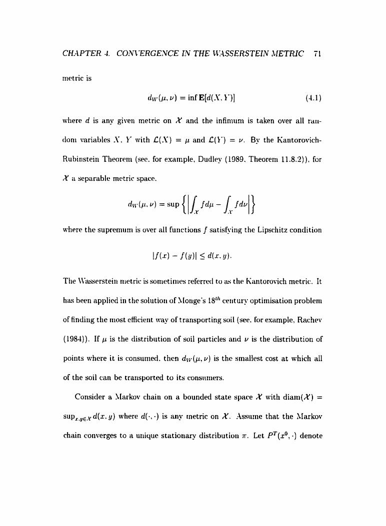
CH.4 PTER 4. CON\'ERG EiVCE IiV THE \.\[4SSERSTEI.N &fEZ'RIC 7 1

riietric is

<lu&, u) = inf E[d(S, Y)] (del 1

mhere d is any giveii metric on X and the infinium is taken over al1 rait-

tloni variables S. Y with L ( S ) = p and &(Y) = o. By the Kaiitorovich-

Rubinstein Tlieoreni (sec. for example, Dudley ( 1889. Theorem 11.8.2) ), for

X a separable mctric spuce.

where the supremiirn is over ail furictions f satisfying the Lipschitz condition

The \Vaserstein nietric is sornetinics referred to as the Kantorovich metric. It

h a beeri applicd in the solution of Monge's lath ceritury optimisation problem

of finclirig the niost efficient way of transporting soil (see. for enample, Rachev

(1984)). If p is the distribution of soil particles arid u is the distribution of

points mhere it is consumecl. thcn di+, v ) is the smallest cost at which al1

of the soil can be transported to its consiimers.

Consider a SIarkov chain on a bounded state space X with diani(X) =

SUP,,y~.~ d(x. y) where d(- , a) is any rnetric on X. .-\ssume that the Markov

chain converges to a unique station- distribution K. Let PT(xo , -) denote

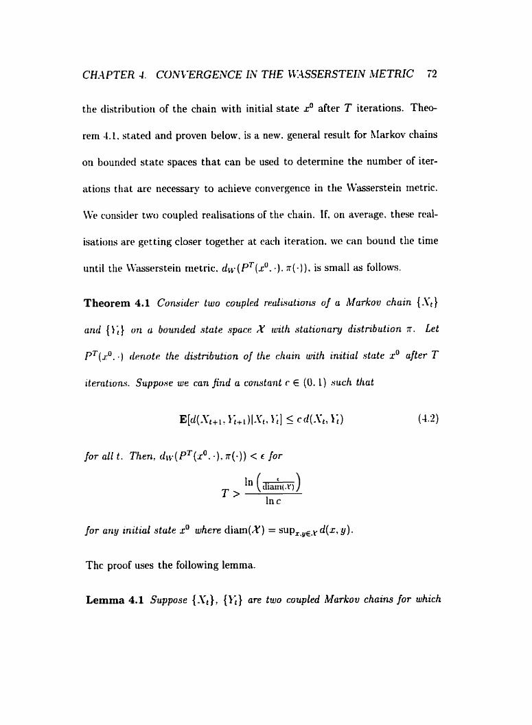
the distribution of the chain with initial state xo after T iterations. Theo-

rem 4.1. statecl and proven below. is a new. general result for hlarkov chains

on bounded state spaces that can be used to determine the number of iter-

;it ions t hat are necessary to acliieve convergence in the CVaççerstein metric.

LVe coiisider trvo coupled rr;rlisations oF the c h a h If. on average. these real-

isat ioiis are gtbt t ing closer together iit racli iteration. WC can bouricl the tinie

until t lie CC~Cil?jsersteiti nietric. drb-(~'r( .P. .). a ( - ) ) . is small as follows.

Theorem 4.1 Consider two coapled riiulisutions of u Markov chain {.Yt}

und ( 1 ; ) on u bounded state space X witlr stutioriary diststnbution R . Let

PT(s'. .) deriotri the distribution o j the clrtrin with initial d a t e x0 afier T

iterritions. Suppose lue can firid a ~ons tan t e E (O. 1) SUCIL tliat

for al1 i. Theri. d i v ( P T ( r o . -). A ( - ) ) < c for

for a w j initial stale r" where diam(X) = s~p,,,,,~ d(z , y).

The proof uses the following lemma.

Lemma 4.1 Suppose {-Yt), (11) are two covpled i h r k o v c h a h for which

CH=IPTER 4. CON\'ERGENCE IN THE Il~A!3SERSTEI.N AlETRIC 73

there exists a positiue constant c such that

E[d(St+i, l;+l)lSt. l;] 5 c d ( S t . 1 ; )

for d l t . Tlirri for nny f i e n T and any -Yq. 1; .

E[d(ST. l>)ldYo, kb] 5 c*'d(~O. 1;).

Proof of lemma The proof follows by induction. Suppose For sornc k

E[d(.vk. ki)I-vo, Io] 5 ?d(.\'u. 1;).

Proof of theorem CVe wish to bound the number of iteratiotis, T. wliicti

gunrantee drr- (~ ' ( .P. *). n(-)) 5 c where ro is ariy initial state. Consider

another realisation of the Markov chain started in r which is it sample frotii

IF. hpplying the lemma,

dll ( PL(r'. -) , K(.)) is less than or equal to c for

Substitiitinp diam(.%') for d( r" . r) gi~res an upper hound on T.

This. if we can fincl a value of c satisfying (-4.2), we can find a boiind

oii tlio i-orivergence tinie giiaranteeiiig the IVasserstrin inetric is less thari a

specified toleraiice c.

4.3 Probability Metrics

Tlirrc. esist dozens of distance measures to qiiantify closeness between two

prot~iihili ty nieaslires (sec. for eaani pie, Rachev ( 1991 ) ) . Hocvever. inost con-

sicieratioiis of the convergence of blarkov chains have used total variation dis-

tance (for csaniple Diaconis and Stroock (1991). Jerrurn and Sinclair (1993).

Tierney (199.1). Tierney (1996)). Recall that the total variation distance

betwen two probsbility nieüsures p and v defineci on X is

If X is finite,

This rcpresentation is half the L' rnetric used by Geman and Gernan (1984).

Sonie au t hors (for exaniple. Tierney (1996)) define total variation distance

as twice our dc+iiii t ion.

Somr of ttir popularity of' total variation distance can bc attributed to

its ability to rxhibit a thresholtl ptienomenori (sce. for exainple. Altloiis and

Diacorlis (1 987)). For niany regiilar eraniples. the total variation distance

Iloreover. the eqiiivalent forrriiilatiori tlrops siicldriily froni near 1 to near O.

1 dr\-(p. P) = - max

'2 lhl'i

wliercl the iiiaxiiiiiitti is taketi over futictioiis h : X -t iR satisf'yitig (Ii(.r)l 5 1.

allows ii boiitid ori total variation distance in tertns of the espected value

of sotrie fiiiictions. .\luch of the success in bounding convergetic<% it i total

variation distancc arises From its coupling characterisation

dTi-(p. u ) = inf P r ( S # 1')

wbere the infir~ium is taken over rancloni variables S and Y whose distribu-

tions are p aiid u respectively. For exarnples of this, see hldous and Diaconis

(1987), Roscnthal (1995b), Luby et al. (1993), and Chapter 3.

To the au t hor's kriowledge, this is the first application or convergence

in the thsserstein metric to XIarkov chain Monte Carlo algorithms. The

klhssersteiri nietric was chosen for this application because of its coiipling

cliaracterisation. Equation (4.1). Total variation distance is not pract ical in

many applications on contiriuous state spaces as the total variation distance

betweeii any cont inuous distribut ion anci any discrete distribut ion is a i w q s

1. irrespective of tiow well t hc continuous distribution is approxirtiated by

the discrete tlistributiori. The Wasserstein nietric metrizes convergcrictB iri

distributiori (see. for eraniple. Dudley ( 1989)) rvhile convergence iri total

variation distance is stroriger t han corivergrnce in dist riba tion.

The Prokhorov niet sic

dp(p. V ) =

inf(n > O : p ( B ) <_ u ( B n ) + CI ancl v ( B ) 5 p(Ba) + u for al1 Borel sets B}

wberc Bn = {L. : infgqB d ( r . y) 5 CI) &O metrizes convergence in distri-

bution. Convergence in the CVasserstein metric implies convergence in t tie

Prokhorov met ric becatise of the following relationship (see. for esarn pie.

Huber (1981, p. 33))

d: drv.

The following relationship exists between total variation distance and the

dci 5 diam(X) dTk.

wtiere diam(X) = sup,,,{d(r. y ) : r. y E X}. If X is a finite set there is a

boiintl the other way. If dm,,, = niiri,,,d(r. IJ) for distinct points r. ici X.

t ticri

0 1 1 ;in infinite set no such relatiori can occur as it is possible for dry to go

to O wtiile drk- reniains fisd at 1. The relatioiiship (4.3) will be proven in

Scctioii 4.5 and applied to givc ari improvccl precise bourid for a result in

Chaptcr 3. For a siiinniary of sonie utlier conirnonly ciscd probability inetrics

aricl ttie relationships that exist arnoiig therii see Cliapter 6.

4.4 Restoring a Grey-Scale Image

4.4.1 The Model and Algorithm

We riow apply the convergence boiind in the Wasserstein metric of Theo-

rem 4.1 to an aigorithm used to restore a distorted image.

Consicler a grid of .V pixels, each of which takes on a value in [O, 11. For

esample a white pixel is O. a black pixel 1 witli values in between representing

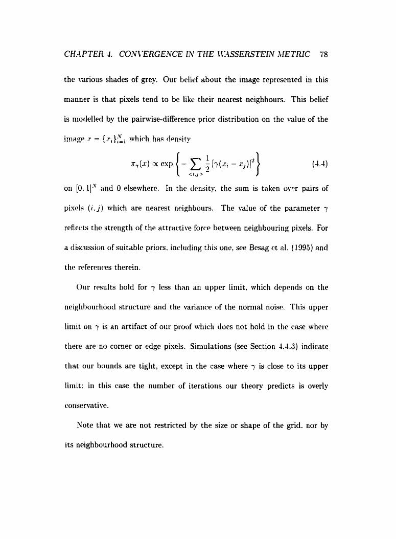
the various sliades of grey. Our belief about the image represented in this

rnaiiner is that pixels tend to be like ttieir nearest neighbours. This belief

is riiodelled by the painvise-difference prior distribution on the value of the

imiigp .r = whirh has h s i t y

or1 [O. 1ILV and O elsewherc. In ttit. ticrisity, the siim is takeri ovv pairs of

pisrls (i. J ) which are nearest neighboiirs. The value of the paranieter 7

reflwts tlic strength of the attractive Force between neigliboiiring pisels. For

a clisri~ssiori of suitable priors. includ irig t his one, see Besag et al. ( 1995) anci

t hc referenres t herein.

Oiir rcsults Iiold for -y lcss than an upper limit. which dcpcncis on the

neigtihocirliooti structure and the variance of the normal noise. This upper

liriiit or1 :i is an artifact of our proof wliicti does not hold in the case where

tliere are no corner or edge pisels. Siniulations (see Section 4.4.3) inciicate

tliat our bouncls are tight, except i r i the case where y is close to its upper

limit: iri ttiis case the nurnber of iteratiotis Our theory predicts is overly

conservative.

Note ttiat we are not restricted by the size or shape of the grid. nor by

its neighbourtiood structure.

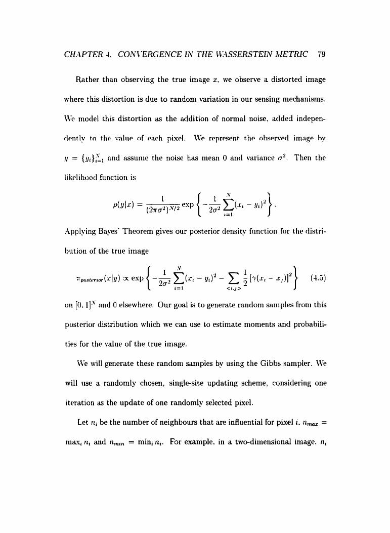
Rather than observing the truc image z. ive observe a distorted image

wtiere this distortion is due to random variation in our sensing rnechanisms.

WC mode1 this distortion as the addition of normal noise, aclded indeperi-

r l ~ n t l y tn thr v n l i i ~ of each pixel. LVI. reprwent. the ohsc.nwl image by

= and assunie the noise has mean O arid variarice 0'. Theti tiic

li kelihoad funct ion is

Applying Bayes' Theorem gives our posterior derisity fiinctiori for the clistri-

h i t iori of t lie t rue image

oii [O. l]*y iiiid O elsewhere. Our goal is to generate random sarnples froni t his

posterior distri but ion which we c m use to estimate moments and probabili-

ties for the value of the true image.

CVe will generate these random samples by using the Gibbs sampler. CVe

will use a randornly chosen, single-site updating scherne, consiclering one

iteration as the update of one randomly selected pixel.

Let ni be the number of neighbours that are influential for pixel i. n,, =

n i u , ni and n,,, = mini ni. For example, in a two-dimensional image. ni

is tisiially 4 or 8 for interior pixels. and, correspondingly. 3 or 5 for pixels

on the houndaries, and 2 or 3 for pixels on the corners. From (4.5) the full

coriditional densities for pixels ri, given the values of al1 other pixels. r-,.

tincl the cibserved image .II are

on [O. l ] end O elsewlicre. The pixels { x j . j 5 i) are those wliicli are neigh-

boiirs of the ilh pixel. N o t ~ tliat this is the restriction to [O. LI of the nor-

mit1 distribution witti nipiiii (O-? + n , f2 ) - ' (Ü'IJ, + 7' x,_, r,) aud vari-

ance (O-' + r r ~ ~ ) - ' . The algorithrii proceeds by choosing an initial state.

and iit cach iteration. randoriily sclecting a pixel for iipclating üccording to

(4.6). Tu sarnple from the riormal distribution restricted to [O. 11. wve use an

iriverse normal cumulative distribution function approxirriat ion. transform-

ing the uniform random number as described in Fishman (1996. p. 152)

for restricted sanipling. For an iiccurate approximation to tlie inverse nor-

mal distribution function. sec. for example. Thisted ( 1988. p. 332). Tliis

IIarksv chaiii simulation continues until the result can be assumed to be

apprminiately a sample from tlie stationary distribution (4.5). Note that

other methods, such as rejection. are possible for sampling from the normal

CH-4PTER 4. CONVERGENCE IN THE C'CISSSERSTEILV *\IETRIC 81

distribution restricted to [O. 11. However, in obtaining our convergence re-

suit giveii in Section 4.4.2, we require that our kIarkov chain is monotone.

For this reason it is necessary to use a sampling method sucti as the inverse

traiisform rnethod whicli preserves the order of the uniforni randoni variables

in the corresponding sarnples frorn the clistributiori of interest.

4.4.2 The Convergence Result

For rl. r' two configurations of our image space, we use the following distarice

furict ion

The following bound ori the convergence time holds for small values of the

prior pararrleter mhen there are edge effects. If eacti pixel has the sanie

niiniber of rieigtibours. for esüniple a n image that has been wrapped around.

therc are no restrictions.

Theorem 4.2 Consider an image of ;V pixels, each taking a value in [O, 11.

and rnndonzly distorted b y the addition of N(0,u2) noise independently at

euch pixel und restored using the random scan Gibbs sumplrr algorithm. The

distance between the distribution of the lC1arkov chain and its stationaq dis-

CH.4 PTER 4. C'ONI'ERGENCE IN T H E 'SC:4SSERSTEIN METRIC 32

tribution will be less than in the CVusserstein metric at iteration T for

where n,,,,, is the muxirrrrrrri mer al1 p i d s oJ the nuin ber o,f influential nezyli-

bouring pixels. n,,,,, is the rriinirnlirrr over al1 pwels o/ the nuniber of inpuen-

tinl neighbouririg pixels. und is the ualue u/ the smoothing purameter /rom

the yrior distributiorr (4.4) .

Before we prove ttiis thcorem, wc will sliow t h coupled realisations of

the hlarkov chai11 arc rrioriotonc as defined in Section 2 . 4 2 and state aiid

prove a lemina about the means of the norrrial distribution restricted to

[O. 11. This allows us to sirnplify Our calculation of the distance between the

current states of the ctiains started in the maxinial and in the minimal states.

A partial ordering exists on the state space where one configuration is

greater tlian or ecliial to another rvhen eacli corresponding pixel has ttiis

ordering, Le.

4

C'ricler this partial order there exists a unique minimal state, rmzn = 0, and

a unique rnavimal state. .Pax = 1. al1 pixels white and al1 pisels black.

rcspeîtively.

Lemma 4.2 Consider tuio cuupled realisotions of the Markou chuin described

iri Section 4.4.1. The pardial order is presewed uiter trunsitions. i .e . if

x t - 1 ,higtr > xt- 1,Low st.htgh > Jt.luiu - - , w h e r ~ xt,h''h is the d a t e of the chain

with ini t ld state .rh'gh ut tirne t .

To prove this lenirna w require the followitig Iminia. wliich me quote iri

tlic Forni given in Roberts atid Rosentlial (1999. Leriiriia 5 ) .

Lemma 4.3 Suppose thut pl urrd pz are tlruo probability rrreasures on R. such

thut tliere is u uersion of the Rudon-Mkodym deriwutt~ue R ( r ) = p2 (dx) / pi (dx).

wlrich is a non-decreusirrg function. Suppose also thut / is a rion-decreasiny

junction front IR into R+. Let E,, i = 1.2 denote e q ~ c t a t i o n s wzth respect

to the t#wo measures pi. i = 1. '2. Then for any set -4 for which the followzrrg

coîrditional expectations exist?

Proof of Lemma 4.2 Consider two coupled realisations of the Markov chain

started in intial states r h z g h and xi". At each iteration one pixel, say the ith,

CHAPTER 4. CONVERGENCE IN THE \\:-ESERSTEIN METRIC 84

is randonily chosen for updating as a sarnple from the full conditionals (4.6).

For each coiipled realisation, we use the same uriiform raiidom number and

gencrate the sample using an inverse clistribiition function approsirnation.

The hi11 conditionals at iteration t are N ( c r f . JT) ciistributioiis restricted to

[O. 11 where

is tlic sarne for the chains regarciless of initial state and

l ,high is tliffcrrnt for the two coiipled chains. C \ é 1ahc.l the two values cr, aiid

a ' WC let T.V(af, JI) represent the .t'(a:, . f ) distribution restricted to

[O. LI.

We will first show that ocir Markov diain is stocliastically nionotorie.

Then updating using the inverse normal distribution function as ciescribed

in Section 4.4.1 preserves the order in our couplcd chains after each update.

Our 'iIarkov cliain is stochastically monotone if. whenever 1'- L.h'gh > - xt-l+fow!

for any a E R where

t,high t,high -=a - T N ( a i , ) and ~ 1 ~ ' - 5 T:v(~:"". bf).

is iin increasiny furiction. Application of L m i r ~ i i i 4 . 3 gives (4.8). giving

stochastiç nioriotoiiicity (4.7).

Csirig the inverse normal distribution fiiriction For uptlüting as describcd

iii Section 4.4.1. stoctiastic ~iionotonicity ensures ttiat the partial ordrr is

iriairitained after trarisitioris of the Markov chain. To sce this, let < be the

ilniforni raiidoin nurnber used for updating both chains and suppose site i is

the site being updated at iteration t. The new values of the ith pisels are

x-. lr tgt l . r'.'"". choseri to satisfy

CH.4PTER 4. CONC'ERGENCE I N THE \CI4SSERSTEIN LLIETRIC 86

The following lemma shows that the difference in the mean of normal

distributions with the same variance is at l e s t as great as the difference iri

t f i ~ rriean of the corrcsponding normal distributions rcstrictcd to (O, 1). It

mil1 lit. used in the proof of Theorem 4.2.

Lemma 4.4 Let e J ( a ) be the meun of the T.V(a. J') rliatrib.ution. uthich LS

the .V(cr. J2) distribution restncted to [O. l]. If ah'"" - dm. t hen

Proof of Lemma 4.4 We will first define the following qiiaritities:

- Let fJ(n) = e&) - CL.

- Let tn j ( s . t ) be the nieüii of the .V(O, J') distribution rcstricted to [S. t ] .

- Let py(.s. t ) = Pr(Z E [S. t j ) where Z - .V(O, y).

Now

And if .s < t < u

Yow for s < t < u.

Now let s < t < s + 1. Then - t < - s < -t + 1 < -s + 1 aiid using (4.9)

CH-IPTER 4. CONYERGEL'VCE IN THE WSSERSTEIN METRIC 88

Since this holds whenever s < t < s + 1, it also holds for any s < t by

breaking the interval [ S . t ] up into sub-intervals whose width is smaller than

one.

Proof of Theorem 4.2 It suffices to consider the nuniber of iterations iintil

coupled chains started in the mai inal ancl niiniinal states have converg~tl to

within c toleraiicc in the Wuserstein metrir. This ensures corivergence of a

chain started in atiy otlier state to the stationary distribution. To sec this.

suppose the state r is a sample from the statioiiary distribution i~ and ra is

an? other stüte. Theii

where the first inequality is the triangle inequality and the second follows

from monotonicity of the coupled chains and the definition of the CVasserstein

metric (4.1). Note also that d ( ~ ~ ~ , r * ' " ) = diamX.

CH.4PTER 4. C0:VVERGEiVCE IN THE CK4SSERSTEIhi IVETRIC 89

Then to get Our rcsuit. we need to find a constant c E ( O . 1) so that

E [d(lt+ 1,mar =t+ 1,min ) lZt,rnax < <l(xLmaz, IL.mln) T . 2 y m t * ] -

where the first inequality uses Lernma 4.4. In the expression

CH.4 PTER 4. CON\ 'ERG ENCE IN THE It:4SSERSTEIiV AIE TRIC 90

the differencr in the values of the kth pixel appears nk times. once for each

pisel i that it neighbours. Thus

The coeffkierit of the right side is less tliari 1 for

1 = r , i e each pixel has the saine number of neighbours so

tbere are no edge effects. the result in the theorem holds for al1 values of y.

In the linlit cr + oo, we have no information from the observecl image

and rio result holds (the upper liniit for the range of 7 is O ) . If a = 0. the

result holds for al1 A/.

The fourth column of Table 4.1 shows the theoretical results for various

values of N. c. n,,, n,in, y and o. Values are compared to a 32 x 32 grid

CHAPTER 4. COiV\'ERGENCE IN THE t'L4SSERSTElN tf ETRIC 91

with 6 = 0.1, rtmar = 4. rin,*, = 2. 7 = 1, and CJ = 0.2. The required niiniber

of iterations until convergence, T , can be seen to vary with the size of the

image. N. and the value of the prior smoothing parameter. 7, but varies little

\vit h t lie ot her pararrieters.

4.4.3 Results from Simulations

The final rolumn of Table 4.1 gives the nurnber of iterations ttiiit were re-

qiiired for the .\larkov chnins started in the maximal arid mininial statrs

tr, conic withia for several differerit siriiiilations. Sirriulat ions were writteri

in C. Sariiplrs frorn the t runcated riornial tlist ribiit ion w r e ohtairiccl iising

the irivrrse normal distribution fiinction approximation of Thisted (1988. p.

332) wit h the adjustriient for restricted saniplirig given ty Fishnian ( 1996,

p. 132). In eacii case. the original image consistcd of four overlapping rect-

angles. in hlack. white, and two siiades of grey. While these siniiilatioris to

üpprosiniate coalescence do not rneasure the same quantity as our nietric.

the closeness of the siniulated coalclscence t inies to the t heoretical niiniber

of iterations required. with the exception of the case where the va!iie of y is

close to our upper limit, is reassuring. Note that one simulation (the first

listecl) required niore iterations t han the t heoret ical value; Our bounci is on

CHAPTER 4. CONVERGENCE I N THE CWSSERSTEIN JIETRIC 92

the niimber of iteratioris required until the mean distance is less than t. and

does not giiarantee the distance on any one malisation will be that srnall.

The siiniilation of 1000 restorations witli y = 1 described iri the next para-

gnipii giws a Letter iiidicatiuii tliat our tiiwry is giviiig a tiglit Luuiiîl uii

the act iial coiivergence time of the Wsserstein nietric.

U't* siriiulated 1000 restorütions of our 32 x 32 pixels iiriage. clistorted by

riornial noise with standard deviation 0.2. Each simulation corisisted of two

realisatioris of our Narkov ctiain, started in the maximal arid rr i ir i irr ir i i states.

Wc set t l i ~ prior smoothing paranieter 7 at 1.0 and t tic iieighbourt~ood struc-

ture siich ttiat interior pixels were influcnced by their Four ncarest neighbours.

These simulations were each ruri for 11096 itcrations, the riuriibcr our the-

ory recliiires for convergence to witiiin e = 0.1 precision ici thc hssersteiti

metric. For each siniulation, the actud distance between the states of two

hlarkov chains after iteration 11096 was recorded. The distribution of these

distarices \vas rigtit-skewed. with a mean of 0.07769, as conipared to the pre-

cision of 0.1 that we requested in our determination of the number of runs

required. CVhile rnost of the distances were below this, there were ma- high

values. iricluding 12 values greater than 1.0. Approximately one-fiftli of the

simulations (216 of 1000) had not coupled to within 0.1 precision.

CH.4 PTER -1. CON\ 'ERGENCE Ih* THE CWSSERSTEIN hl ETRIC 93

T heoret ical

value of T

11096

808

4885 13

14658270

Number of iterations

required in siniulation

Table 4.1: Convergence tirnes for the restoration of a grey-scale image.

Figure 4.1 gives ail esample of the image restoration process. Figure

4.l(a) shows the true image. drawn on a 32 x 32 grid. It was randornly

degradeci with X(0, O. 15') noise, added independently to each pixel. The

degraded image is shoivn in Figure 4.1 jb). In the prior distribution. 7 vas

set at 4 and neighbours were considered to be the pixels above. below. and

beside ( r i , , = 4 and n,,,, = 2 ) . The specified accuracy \vas c = 0.1. Xote

that this error is clistribiited across 102-4 pixels. The algorithm was run for

58081 iterations. the tlumber that our theory reqiiires for convergence to

wit liiri c accuracy. and oiir initial state wüs e w r y pixel black. Figure -4. i (c)

shows the mean of 10 iiicleperident saniples from the posterior distributiori.

4.5 Results for the Restoration of a Binary Image

The case where the image is a grid of binary pixels was considered in Chap-

ter 3. Consider a configuration {.q) of 'i pisels whicli take on values -1-1

or -1. The following prior distribution. the king model. assigns greater

probability to configurations where neighbouring pixels are alike

CHA PTER 4. CON\'ERGENCE IN THE CK-1SSERSTEI.N METRIC 95

Figure 4.1: A simulated restoration of a 32 x 32 image. (a) true image: (b) observeci image: ( c ) the mean of 10 independent samples frorn the posterior distribution.

CHAPTER -1. CONVERGENCE I N THE CK4SSERSTELN XfETRIC 96

where the sum is taken over pairs of sites ( 1 , j) which are nearest neighbours,

.i is ü positive parameter, and Z is the nornialising constant.

In Chapter 3, precise 0(!V2) bounds were found ori the convergence time

of the Gibbs sarnpier for sampiing from t his prior. and For sümpling from the

posterior riiodel obtained by conibining this prior with observecl data. The

obscrved data are ciistorted images O btained from the t rue image by ranclom

dis tort iori rnechanisms. Results were founcl for two distort iori rriechanisms:

additive normal noise arid randoni flips. Csing coiipling, upper bounds were

obtained on the necessary number of iterations uiitil total variation distance

is less than e of the form

2CV2 -(1 - loge) f (4

where /($) is an easily evaluated. knowri positive furiction OF the parameter

of the prior distribution. These bounds hold for values of 3 below a given

thrcshold. The function /(,LI) differs witli the distortion tnechaiiism.

The distance function considered in Chapter 3 was the nuinber of pixels

wvliicli differ in the two chains. The relationsliip of the function f (j) to the

change in the distance function allows us to apply the calciilated values of

f (3) from Chapter 3 to get a result for convergence in the Wassersteiu i~ietric.

The theorem that follows gives these results for the three cases considered in

C'HA PTER 4. COiVVERCXNCE I N THE CCI-ISSERSTEIN ME TRJC 97

Ctiapter 3.

Theorem 4.3 Consider the use of the random scan Gibbs sarnpler for the

rrstoration of an image O/ .V pixels in arbitrary dimension where each pixel

ïuri take on the ualues { - 1. +l } und is infiuenced b y its TL nearest neighbours.

The trlyuritlrrn wiil huve coriverged in the sense that the CVassei*steiri metric

i r d l be less than 6 al lime T jor

whcre I(j) and the possible values of ,3, the parariieter from the C s i q rrniodrl

pi-&or. ( L T ~ yiven us follouts for tlrree cases:

1. The distribution O/ interest is the Ising rnodel. Eyuotion (4.12). Then

2. The dist~ibution of interest zs the pouterior distribution with Ising mode1

prior und the obsemed image is modelied as the true image with each

with probability a. Then

CH.4PTER 4. COM1 'ERGElVCE W THE bK4SSERSTEIX LLIETRYC 98

10 r

where ka = ( 1 - a ) / n + n/(l - a).

3. The distribution of interest tu the postefior distribiltion ivitlr Isiny rnodel

prior und the obserued inlaye is trrodelled us the t m e imuyr: with :V(0.02)

rroise a d d d indepertdently to each pixel. Then

where is the vafiie 01 the .smallest ( in absolute ualue) obsenied pixel

Proof In the proofs of Tlieorenis 3.3, 3.4, and 3.5. it was shown how the

expected change in the distance fiinction in one iteration can be espressed

as ttie product of -y and the current distance. Thus.

CH-4PTER 4- COXC'ERGENCE IN THE \KClSSERSTEIN iLfETRIC 99

This expression can then be applied with Theorem 4.1 to give (4.13). The

expressions for f($) and the values of d which ensure that f (!i) > O for

the tliree cases are calcillateci in the proofs of Theorems 3.3. 3.4. and 3.5.

respect ively.

By m i o r series expansion of the above results. it is eûsily seeii ttiat the

bouiids on the coriwrgerice tirnes are O (X ln 'l).

This resiilt also giws an upper bound on the tinie until total wriatioti

distarice is less than because of the following relationship.

Proposition 4.2 On u jïnite set X, the Jollouring relationship exzsts betioeen

total ~uan'ation dzstunce u r d the Wusserstein metn'c:

urhere cl,,,, = min d(s . y ) urhere the minimum is taken over ail possible pairs

of distinct points r. y in X.

Proof For p. u two nieasures on X and .Y. t' random variables with L ( S ) =

p and t ( Y ) = u,

CH.4PTER 4. C'ON\~'ERG'EiVCE IN THE CCI4SSERSTEIiV ICIETRIC 100

and

d;-l.(p. u ) = inf (Pr(X # Y ) } = inf{E[l~s+yl]}. .!-,Y -\ ,\

But

d(-Y.t.-) 2 &inl { . \ .+> . ) .

We can now g ~ t the Eollowiiig bounds for corivergence in total variûtiori

rlistitnce.

Corollary 4.1 The ruridom .scan Gibbs sampler ulprithrns for sarnpliny Jlatrr

the models Jescribrd in Theorem 4.3 wzll have co~werged in the senae thut the

total variation distance wrll be less than ut timc T for T greuter than the

uulues giveri in euch uf the three cases beloaw:

1. The distnbutiori of iriterest is the Isirig rrrodel. Equution ( 4 . 1 2 ) . Then

2. The distribution of interest i s the postenor distribution un'tli Ising mode1

pnor and the obsemed image is modelled as the true image with each

pizel zncomectly obserued ~12 th pro bability a . Then

9. The distribution of interest is the posterior distribution with Ising mode1

prier and the obserued image i s modelled as the true imuge wittr X(0. 02)

noise udded irrdependently to eoch pixel. Then

where y,n,, is the value o/ the smullest (in absolute value) obserued pixel

- e - ~ r n : n /O' + e- '~rn,n/u2, and k.,,,,,,,, -

Proof Our distance function d ( S , 1') is the nurnber of sites where S. 1' differ.

Thus dmin = 1 and the Wsserstein results of Theorecri 4.3 give immediate

upper bounds on convergence in total variation distance. I

-1s an example. in the case of normal noise. for a 32 x 32 grid with pixels

influencecl by their 4 nearest neighbours. if cr = 0.3. ymin = 0.1, ,3 = 0.1,

and É = 0.1. the number of iterations required for convergence in both the

C W PTER 4. C O M 'ERG ENCE I N THE 'ICISSERSTEIN ME TRIC 102

\V~ssersteiii riietric and total variation distance is is 36281. In Chapter 3 our

upper bound on the convergence time was 72246394.

4.6 Application to Exact Sampling

Exact sanipling algorit hrns (Propp and Wilson 1996, Fil1 1998) have receritly

generated a grmt deal of iriterest in the 'iIarkov ctiaiii Monte Carlo literaturc.

In partirular. t tie algorithm of Propp and CVilsori (1996) involving the coiicept

of coii plirig-frroiiri- t he-past has been applied and extended to a nuniber of

diffrreiit applimt ions. For a monotone l Iarkov chain for whicli t here exist

iiniqiie niaxinial üticl minimal elements. the algorit tim irivolves riinnirig two

realisations of the hlarkov chain started in eacti of thcse states froni time - t

forward. If the chains have coupled a t tinie O the resulting statc is exactly a

sample Froni the distribution of interest.

If the algorit hm is monotone as defined in Section 3.4.2 and the distance

between maximal and mininial states is equivalent to the diameter of the

space. our throry For convergence in the iVasserstein metric can be appliecl

to giw a boiind oii the expected running tinie of the coupling-froni-the-past

algoritlim. As discussed in Chapter 3 and Section 4.4. the image processing

examples in this chapter are exmiples of monotone blarkov chains.

Our ttieory for convergence in the Wasserstein metric assumes that cou-

pling of the masimal and minimal states of oiir nionotone chain to within

tolerarice is adeqiiate. This idea was considered by Moller (1999) in the

contest of applyiiig exact sanipling algorithnis using coupling-from-the-past

to continuous state spaces. Moller considerecl chairis which cri- not have

kt rriai~irnal state. but for which a dominating chain c m be constructed.

Slollrr's coiipling-frorn-tlie-put algorithm reqiiires tlie clorninating chairi to

corric within of the Markov chain starteci in the niinirrial state. wherc c is

the arcuracy specifiecl by the user. He sho~ved that this algorithm gives ari

esact saniple froni the stationary distributiori to within e accuracy in a finite

t irne.

The distribution of tlie tirne to couple into the future is the same as the

distribution of the smallest t such that chains started at time -t will have

couplet1 at time O (Propp and Wilson 1996). Thus our results can be used to

givc an iiidicat ion of how far in the past it is necessa- to go back to achieve

approxiniate coalescence at time O in bloller's algorithm.

The binary image restoration algorithm of Section 4.5 is an example of a

finite state space, monotone chain, so the coupling from the past algorithm

of Propp and Wilson (1996) can be immediately applied. Tlie bounds of

Theorrm 4.3 give an indication of the required starting time in the p s t

necessary to arliieve coalescenctb at time O.

Fur uiiifuriiily ergodic Morkov cliaiiis. i t is pussihle tu acliirvt. exact cu-

alescerice c m writinuous state spaces by the application of the rriiiltigamrna

roiiplt~r of h r d o c h and Green (1998). or. iis iridicated by SIcllcr (1999) fol-

lowing a suggestion by Duncan !durdoch. a hybrid of the niultigarnma coupler

aiitl Slollw's idgorithni. Anuther approacli to achievirig exact coalescence on

coritiriiioiis stittc. spaces involves the irisertion every kth (for example. A: = 10)

iteratioii of a .\.letropolis step with updates of the forni suggestecl by Yeal

(1999). Iri tliis step. a hyper-gricl is placecl on the state space with its ori-

gin detmriirirul raridonily. Tlie lengtli of the sidcs of the Iiyper-boses of the

gricl is fixt-cl. The proposal state for the SIarkov cliain is the centre of the

box containing the current state. If the current States of two chrins are in

the sanie box. th- will have the sanie proposed new state, and a positive

probability of exact coalescence.

Chapter 5

Using Auxiliary Simulation to

Approximate Theoret ical

Convergence Rat es

5.1 Introduction

In this chapter. we examine how auxiliary simulation can be used to tind

approxirnate values for the parameters of the Slarkov chain 'Iloiite Carlo

algorithris that must be calculated in ordcr to apply our theoretical con-

vergence resul ts. In particular, we use auriliary simulation to calculate the

pararneter c frorn out result for convergence in the Wasserstein metric as

described in Chapter 4. The same approach can be used to calculate the

parameter ci used in Chapter 3 for Our convergence resiilts in total variation

distance.

Recall Ttieorerri 4.1. Suppose {St }, (1 ; } are tao coupled realisat ions

of a lIarkov chah on a bounded state spacr X. If we can find a constant

c E (O, 1) sudi ttiat

for al1 t . theri a lIarkov chah started in an- initial statc will have convergeci

in ttic sense that the FVitiserstein mctric betwecn the distribution of its strttc

iit timc T and the stationary distribution will be less than e for

where diani(X) = sup ,,9,, d(+, y) .

Calculating the valtie of c is the difficult part of applying this theoreni.

In Chüpter 4 we calculated it For an example wvhere the Gibbs sampler was

used and the full conditional distributions wvere normal distributioiis trun-

cated to [O1 11. \Ve also showed tiow calculatioiis in Chapter 3 can be applied

to calculate c for an example using the Gibbs sampler where each compo-

neiit caii take only two values. For niore cornplicated algorithnis. it rnay be

prohibitively difficult or perhaps impossible to calculate c analytically.

-4s ail1 be demonstrated, our ausiliary simulation approach givcs a rea-

sonnbie estimate for c for an exaniple for which we have an analytic d u e .

Howcvrr. it c m riot provide the giiararitees that a calculated value would.

Oiir iiiiti is to bridge the gap b e t ~ v ~ c ~ ~ i the theoretical results of Ctiapter 4.

wtii(:li iiiay be difficiilt to apply to coiriplex models. and rvhnt is reasonable

to ciirry out in practice.

..\ siiiiilar approacli to bridgirig the gap between tiieory and practice is

givrri in Cowles and Rosenthal (1998). Iii tliat paper. Cowlcs arid Roxiittial

describe how auxilary simulation ran ht. iised to verify the coiiditions iind es-

tiniate the paranieters for the theoretical resiilts in Rosenthal (1995b). Ttieir

work is rstended and refined in Cowlcs (1999) in the context of hierarchical

normal linear models.

I t should he noted that care must t ~ e taken in applying the resiilts of

aiisiliary simiilation to calculate the convergence time. Iri order to find the

true value of c. we must find the supremum of the value describecl in the next

section over al1 pairs of initial states. It must be recognised that some part

of the state space may have been missed in the choice of initial states for

wliich auxiliary simulations are carriecl out. However, our example suggests

that our approach works reasonably well. Another limitation of our method

is that it is very cornputer intensive.

* l n advantage of t his niet hod is t hat. unlike convergence diagnostics. the

auxiliary siniiilations we are perforniing to estimate the convergerice tirne do

not bias the final results of the hlarkov chaiii Monte Car10 algorithni ntiich is

ruri inclependently using the nuniber of iterations suggestecl by t hc aiixiliary

simiilat ion.

In Soctioii 5.2 ive outliiie the niethocl we recomniend For carrying out

siniulatioris to estirriate c. In Section 5.3 wc estimate c for the grey-scde

rrioclel froni Section 4.4 which we compare with out calculateci iipprr hounci.

O t her examples including models wi t h ot her prior distributions for which

we have no analytic results are being investigüted ancl will appear in future

work.

5.2 Suggested Approach to Obtaining an Es-

timate of c by Awiliary Simulation

Siriiiilations to estimate c,., stioold be carried out for a variety of states r aricl

y. For exaniple. we cati geiirratc r and g randomly pisel by pisel. \\é should

iilsi> coiisidcr pairs of stiites that are very close together. vcry far apart. and

stattbs tliat are highly probable a prion'.

\\*P reconirnerid a two-stage approacfi. In the first stage. a variety of pairs

of initial states is explorecl. with the goal of identifying wtiich initial statcs

I d tu the largest value of c,,,. In the second btage. nTe gencrate more values

frorri the idcntified states in order to get an error estimate.

Eqlorutory step: Froni each pair of initial states. sirnulate a number. .V.

of oiie-step iterations. The estimate of c , , ~ is the mean of tlie .V ratios of the

distance apart iifter the iteration to the distance between x and y. LV should

br chosen so tliat the standard error in c,,, is appropriately small. Note

that for random scan algoritlims. a better estimate of c , , can be obtained

by updating each pixel NI times. with N1 chosen so that the variance of the

rnean distance ratio for each pixel is as small as desired. The estimate of

CX .Y is then the average over pixels of the average distance ratio per pixel.

Any one estirnate for c rnq owr-estimate its true value because it is possible

for pixels to grt furtlirr apiirt as weil as cioscr togetlier. However. it is

riot desirable to over-estiniate c* by a large amount as an overly conservative

estiniate will indicate tbat ari iirireasonably large niiniber of iterations is

ntwssary to achieve corivergence.

Error estimttte; ,\ri estiniatc of the error in c can be achievrd as follows.

Foriis on the initial states tvhirh gave the largest estirriatcs for in oiir

esplorütory step. Rancionily gerirrate .V2 pairs of initial states and take the

mÿsirriiirri of the correspondiiig wliies of c,,,; this maximuni is an estimate

for r. Do this tinies. The .Vr3 estiniated values of c generated in this

mariner iire indcpendent arid identically distributed. Take as our estiniate

of r the upper limit of the 95% confidence interval of the nieari of these

estirnates. When rounciing it is appropriate to be consemtive and always

round up.

5.3.1 The Grey-Scale Image Restoration Problem with

Quadrat ic Difference Prior

We riow use iiuxiliap sinidation to estirnate the value of c for which we cal-

ciilatecl aiialytically an upper boiintl in Section 4.4. We set the values of the

parameters as 7 = 1. O = 0.2. and .V = 1024. Our image is two-diniensional

with a neighbourhoocl structure where eacti pixel has üs neighbours the pixels

above. below aiid besidt~. The analytically obtained upper bourid for c in this

case is 0.99917368. The obsrrved image used in this simulation is the sarric

set of overlapping hlocks iised in Section 4.4.

For the exploratory stage. we calculated c,,, for the following pairs of

states:

O al1 bliick and ail shit,e (the maxinial and niiiiimal states)

O a soiid-colourecl grey square surroiinded by a lighter shade of grey and

a lighter version of the same image: these states have high prior prob-

ability

O rancioniiy generated inde pendent pixels

a states that are close together generatcd bu:

- starting from al1 black and al1 white, running two couplecl realisa-

tions of the hlarkov chairi for 8300 iteratioiis and using the states

ilt that point as the states x. y

- ranclonily generating an initial state for r and then changing the

value of one rantlonily selectecl pixel for y

- usirig a liigh prior probability state for r and changing the value

of oiie raridonily selectd pixel for 9

hi each of ttiese cases. it nas necessary to siniiilate .VI = 100 or 1000 it-

mations per pixel in orclcr to cstimate the meün ratio for tliat pixel with

standard error at most IO-.?

The largest values of c,,, were obtained when the states r. y were close

together. so we use tliesc for oiir estiniate. For eacb of the three categories

of states that are close together as clescribed above. we generated the mas-

iiriurri of the values of <;., for - = 100 pairs of initial states X3 = LOO

tinies. The confidence intervals For the mean of these i.i.d. maxima are

(0.999138032748.0.999158037252), (0.9991479733.0.9991485927),

and (0.9991595904.0.9991598076). Thus we take as our estimate of c 0.99916.

Büsed on this estimate. and setting Our tolerance for convergence in the

CL~sserstein metric to be 6 = 0.1. we corrclude that 10989 iterations are re-

qiiired for convergence. For cornparison, our theoretically obtained upper

Iiourid lor c ka& tu a requirenietit of 11 171 iterations. or 1.7% more itera-

tions. It shoiild be noted that our theoretical residt is aii upper bouiid on

the triie convergence tinie t tiat rnay be overly conservat ive.

Chapter 6

Probability Metrics

6.1 Introduction

Stuclyirig t lie convergence of SIarkov chah Sloiitcl Car10 slgorithnis to t heir

stat ionary distribut ions recluires a clioice of a probability rnetric to rneuure

that corivergetice. There are a host of metrics available to quantify the dis-

tance between probability measures. each with pürticular properties which

make theni theoretically interesting, or useful in sorne applications. In this

chapter. we çollect in one place some of the most widely used metrics and

summarise the known relationships between them in a handy reference table.

We also provide some new bounds between several of the metrics.

An encyclopedic and dense account of probability metrics is given by

Rüshev (1991). aiid we do not intend to duplicatc Iiis accouiit here. By

coritrast. this chaptcr is limited to nine chosen metrics. Eight appear often

in accoiirits of probability riirtrics; the niricti, the discrepiiricy irietric. is less

wdl-kiiown but is incliicled because of its applicability to problems in wliich

utlicr nietrics are riot suitable.

\\é liniit outselves to nietrics between probability niaisiires (simple met-

n c s ) rat ber t han t lit. hroacler context of niet rics bet weri randorri variables

( tompourid metncs).

This cliapter is orgariized as follows. Section 6.2 lists riietrics in wide iisc

iiiiioiig probabilists and statist iciaris. Section 6.3 discumes bounds betwcen

tlirrri. Sorne esarriplrs of their applications are describeci in Section 6.4.

6.2 Probability Metrics

Ttiroughout this chapter. let R be a coniplete separable metric space, and let

t3 be the Borel a-ûlgebra on R. In àIarkov chain Monte Carlo applications. R

is the state space of the SIarkov chain. Let M be the space of al1 probability

rneuures on (0. B ) . CVe consider convergence in M under various notions

of distance. Some of thesc are not metrics, but are non-negative notions of

"distance" between probability distributions on R t hat are oRen encountered

in practice.

Iii wliat Foilows. let p. P Le two probaliiity trieiisures oti R. Let / aricl

y be thcir corresponding density functioiis (when they exist) witli respect to

an arbitrary rlorriinatirig nieasure A. If R = R. let F. G be the correspontiiiig

distribiition fiinctions. Wien needed. S. 1' will denotc randorri variables on

R such tliat L(S) = 11 ancl L(1') = P .

Total variation distance

1. State space: Q any nieasurable space.

wliere h : R -+ R satisfis Ih(.r)l 4 1. For a countable state space R.

the defini t ion above becomes

which is half the LL norm between the two measures. Some authors

(for exaniplc. Tierney (1996)) define total variation distance as twicc

Our definition.

3 . Note that rvhcn R is a continuoiis state spacc. the total variation dis-

tance is often not suituble, siilce the distance between a discretc ancl a

continuoiis protmbility nieasure is 1.

4. Total variation distance does not nwtrizc weak convergence.

5 . Total variation distarice lias a coiipling ciiuracterisation:

Uniform (or Kolgomorov) metric

1. State space: R = R.

2. Definition:

3. The Uniform rnetric does not metrize weak convergence.

CH.4PTER 6. PROB.4BILITIW ii1IETRICS

Lévy metric

1. State space: Q = R.

2. Definition:

dL(F.G) = inf{c > O : G ( r - e ) - c < F ( r ) < G ( x + e ) + L X t. E}.

3. The Lévy nietricr metrizes weak convergerire:

4. \ik çan riow define an r-neighbourhootl of F: .VF(F) = (G : d L ( F . G) 5

€ 1 .

5 - This nietric clepends on the inetric on R and is not scale-invariarit.

Prokhorov metric

1. Statc spnce: R nny nieasurable metnc space. (This is the analogue of

the Lévy metric for arbitrary spaces.)

3. Defini t ion:

d p ( p , u ) = inf{e > O : p ( B ) 5 u ( B C ) + e for al1 Borel sets B }

where Be = (r : infYcB d(x. y) 5 c}.

3. This metric is not scale-invariant and depends on the metric of R. It

is possible to show that this rnetric is symmetric in p.v (Huber 1981).

Hellinger metric

1. State space: R any nieüsurahle spcice.

2. Definition: the nieüsures p. v niiist have densities f . (I witli respect to

A:

Note: different tests refcr to differerit versions of this nietric. CVe fol1ow

Zolotarev (1983).

If R is a couritable space this reduces to

(Diaconis and Zabell 198'2).

3. Can he Tactored" in terms of marginals (see Zolotarev (1983. p.279) ).

This makes it possible to express the distance between distributions of

vectors with independent components in terms of the distances between

the distributions of the corresponding components.

4. This nietric does not depend on any nietric of $2.

Wasserstein and Kantorovich metrics

1. State space: R or any measurable nietric space.

2 . Dcfinition: For $1 = R, the Kantorovich nietric is defiiied by

For aiiy scpirra ble me tric space. t his is eqiiivalent to

the siiprerniini being taken over al1 h sat isfying the Lipschitz roiidition

3. This irietric met rizes weak convergence.

4. This nietric is not scale-invariant and it depends on the metric of R

throiigli the Lipschitz condition.

5. By the Kantorovich-Rubinstein t heorem. the Kantorovich rnetric is

eclutil to the Wasserstein rnetric:

where the infimum is taken over al1 joint distributions J with margirials

p. P. See Szulga (1982. Theorem 2).

Relative entropy (or Kullback-Leibler separation or di-

vergence)

1. State space: R an? measurable space.

2. Drfiriition: if the measurcs p , v have densities f. 9 with respect to A:

For R a countable spiice:

3 . This is not a metric. since it is not synimetric and does not satisfy the

triangle inequality. However, it has many useful properties, such as

heiiig additive for indepeiident processes ( usefiil for produc t spaces) .

X 2 distance

1. State space: R any measurable space.

2. Definition: if the nieasures p, v have densities J . g with respect to A:

d,2 (p. v ) = ln (f - 912 d,,, 9

For a tounttlblc spacc f? this rctluces to:

Note: Reiss (1989. p.98) defines t h e y' distance as the square root of

the ahove expression.

Discrepancy

1. Stato sprice: R any nieasilrable nietric space.

2. Dcfinition:

d&r. Y) = sup 1\43) - al1 closed balls B

3 . Mt hougli it depends on the metric of $2, this de finition is scale-invariant

and does not depend on the %ize"of the space.

6.3 Some Relationships Between Probability

Metrics

Figure 6.1 is a diagraiii u l the relati~iialiips betweeii various prcjbability rilet-

rics cotisidered in this chapter. Sonie of the relationships only liold on soriic

stüte spaces. or for a restricted clüss of nietrics. An arrow froni metric -4

to nietric B indicatcs tliat an iipper bound exists for -4 iri terms of B. The

anriotatioris inmlving functions of r indicate the nature of the rclationsliip

bctwccn the two nirtrics. An r by itself iriclicates the relationship is direct.

i.c. <1 5 d B . ;\ri expression itivolviiig L. is the fiiriction of the hoiiridirig

nictric. B. ttiat givcs an upper bound on .A. For exiirnple. if the arrow Frorn

;I to B is annotetecl with m. then

The dianieter of the space is given by diarn R = sup,,,,, d ( r . g ) ; the

results involving diamfi are only useful if R is boiinded. For R finitc.

dm,, = infITgEn d ( x . y) . The function is described in the result relating

the Prokhoro\r rnetric to Discrepancy Table 6.1 is a key to the abbreviations

for metrics iisecl in the diagrani.

The relatioriships illustrated in Figure 6.1 and any restrictions on them

Figure 6.1: Relationships ainong probability metrics.

Abbreviation

Discrepancy

Hellinger metric

Relative etitropy

Ldvy metric

Prokhorov niet ric

Total mriatiori distance

Cniforni (or Kolmogorov) nietric

CVasserstein (or Kantorovich) rnetric

i' distance

Table 6.1: Abbreviations for metrics used in Figure 6.1.

are summarised below. References are given wliere proofs of these results are

known to appear. Proofs are given for new results.

Uniform bounds Lévy

dL(F . G ) 5 dL.(F. G).

Bounds relating the Hellinger and Total variation dis-

tances

See LeCam (1969. p.36). It follows that when clri is small. the variation

clistance is sniail.

Relative entropy bounds Total variation distance

For couritable state spaces R.

ciTI. <_ &.

This ineqiiality is dile to Kullback (1967). It follows that when d l is sniall,

the total variation distance is sniall.

Discrepancy bounds the Prokhorov metric in special

cases

Th<. followirig theoretri shows how discrepancy rriay he boiindcd by the Prokhorov

tiietric by finding a siiitable riyht-continuous fuiiction o. For t~oiindecl R. O ( € )

gives an upper bouncl on the additional v-rneasiire of the estencled bal1 B'

ovtBr the bal1 B. where B' = {.r : i d g E B d ( r . y) 5 c ) .

Theorem 6.1 Let R be any rrreasu~able rnetn'c space. and let o be ang prob-

a bilit y rneosure sutisjging

4 B ' ) 5 p(B) + N e )

fur d l balls B and co7nplements of b a h B und some right-corrtinuous function

m. Then for any other probability measure p? zf dp(p. y ) = r. then d D ( p . y ) 5

1 + d(x).

For exaniplet if u is the uniform distribution on the circle or line. then d(r) =

2x.

Proof For p. v as above.

And if +(p . v ) = r. then p(B) - u(Bi) 5 .t for al1 .E > r aiid al1 Borel sets

B. Combining witli the above inequality. wc see that

By taking the supremiim over B which are balls or coniplenients of bülls.

Ttic sürric result ni- be obtaincd for u ( B ) - p (B) by notirig ttiat u ( B ) -

p(B) = p ( B c ) - u(Bc) which. after taking the supremurri over B which are

balls or coniplements of balls. obtain

as before. Since the suprerniim over balls and complenients of balls will be

larger than the supremuni over balls. if dP(p, v ) = s, t hen do(p. u) 5 .i-+Q(.?)

for al1 .i > r. For rigtit-continuous Q. the tlieoreni follows by taking the limit

ris .i decreases to x. I

Using this result. one sees thnt for v = L'. the uniform distribution on

the circle or line,

Prokhorov and Wasserstein metrics

Hiiber (1081. p.33) shows t h

for any p. u probability rtic;isures on a coiriplete separable metric sparc wtios~

metric d is boiiricled by L. 111 gerieral. we show that

Theorem 6.2 The CVussemtein and P.?-V~~OTO.V 1rcet7ic.s satisfy

In particular. d p and dii define the same topology.

Proof For any joint distribution J on randoni variables S, Y,

Ej[d(S. Y)] 5 r Pr(d(S. Y) 5 E ) + cliarn(Q) Pr(d(S. 1') > E)

= E + (diam(Q) - E) Pr(d(S, Y) > a)

If dp(p. Y ) 5 E. we ciin clioose a coupling so that Pr(d(S. Y) > E) is bounded

by E (Huber 1981, p.27):

Taking infimum of both sides over al1 coiiplings. ive obtain

To bound Prokhorov t,v \Cÿsserstein, use Varkov?s inequality and clioosc

E such that dcc. ( p . v ) = r2. Tlien

1 Pr(d(S. Y) > 5 ) 5 - E j [ d ( S . Y)] 5 5

C

nliere .J is any joint distribiitiori on S. Y. By Strasscn's tlicorern (see. for ex-

atnple. Huber (1981. Theorcm 3.7. p.27)). Pr(d(S. Y) > r ) < 5 is equivaleiit

to p(B) 5 v ( B E ) + c for al1 Borel sets B. giving d; 5 &-. I

Prokhorov and Uniform are bounded above by Total

variation and below by Lévy

For mesures on R we have the following relations (see Huber (1981. p.34)):

CHAPTER 6. PROBABILITY ME TRICS

Relative entropy bounds X'

Theorem 6.3 The relative entropy d r and y' distance d p satisfy

Proof Sirice log is a concave funct ion, .Jensen*s incquality yields

whwr the second iriequality is obtained by noting tliat

The Wasserstein metric and total variation distance

Theorern 6.4 The LVusserstein rnetric and the total oariation distance sut-

is fv the Jolluuing relation:

where diani(I1) = sup{d(z. y ) : x, y E O}.

If R is a finite set. there is a bovnd the other way. II&,,, = minij d ( x i , x,)

/or points ri in R, then

dmin . dTv <- clk\..

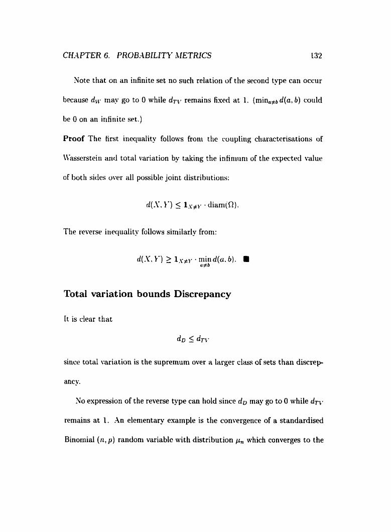
Note that on an irifinite set no such relation of the second type can occur

because ciLl. tnay go to O while dTv rernains fixecl at 1. (minatb d(a. b) could

be O on an infinite set.)

Proof The first iriecpality follows froni the îoupling characterisations of

\V;w;scrstein and total variation by taking the infiniilni of t lie expected \-due

of bot h sides over al1 possible joint distribtit ions:

The reverse incqiiality follows similarly Froni:

Total variation bounds Discrepancy

it is dear that

since total variation is the supremum over a larger class of sets then discrep

ancy.

No expression of the reverse type can hold since do may go to O while dTr

remaiiis at 1. An elenientary example is the convergence of a standardised

Binomial ( n , p ) random variable with distribution p , which converges to the

standard normal clistrihution, v, as n + m. For al1 n < r. dTC.(p,, V ) = 1.

whilc d&,, V ) O as n -t m. Another example is a ranclom rvalk on the

circle generated by irrational rotations (Su 1998).

1)iaconis (1988. pp. 30-34) describes an interestitig example that con-

verges botli iri total variation distance and in discrepuncy, but is kriorvn to

corivcrge at clifferent rates. The example is a simple riindoni salk witti a

raiidorriness tiiultiplier on the integers mod p where p is an odd riurnber. The

procrss is giveri by .Yo = O and Sn = 2S,-, +c, (rriod p) where the c, are ititie-

penclrnt arid icleritic;illy distributeci taking values O. i 1 cach witti probability

113. Ttw stationary distributiori for this process is uni for rn. Usiiig Fourier

ariülysis. Chiirig. Diaconis arid Graliarn (1987) stiow ttiat O(log, p log log, p)

steps arc sufficient to actiieve convergence in total vüriatiori distance. and are

neressary wtien p = U t - 1. for t a positive integer. Hoivever. as proveri in

Sii (1995. pp. 29-31), O(log p) steps are snfficicnt for corivergence in discrep

ancy. In these results. the proportioriality constants are known. SIoreover.

the convergence is qualitatively clifferent in the two nietrics: there is a cutoff

in total variation distance where its value drops quickly from near I to near

0. but not in discrepency.

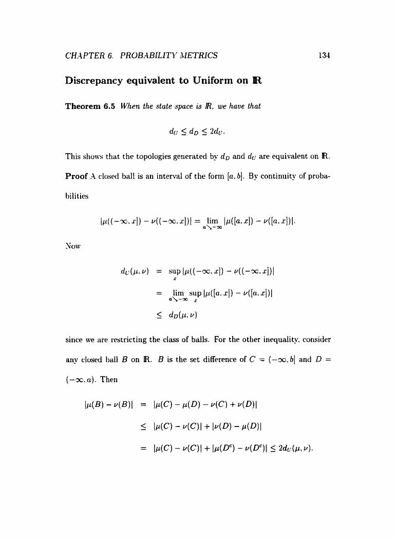
Discrepancy equivalent to Uniform on R

Theorem 6.5 CVlren the state space is R, -we have that

This sliows tliat the topologies generated by ciD and du are equivalent on R.

Proof h closcd bal1 is an interval of the form [a. b]. By contiiiuity of proba-

l~ilities

&(p . u ) = slip Ili((-=. r ] ) - v ( ( - m . r ] ) 1 f

since we are restrictiiig the class of balls. For the other inequality. consider

any closcd t1d1 B on IR. B is the set difference of C = (-30, b] and D =

(-ex. CL). Then

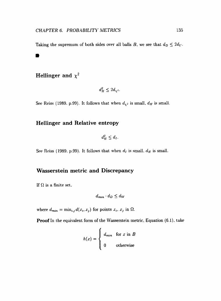
Taking the supremiim of both sides over al1 balls B. we see that d D 5 2dLi.

Hellinger and X'

d i 5 2d,L

Sec Reiss (1989. p.99). It follows tliat wheii d,r is sinall. dH is small.

Hellinger and Relative entropy

dJ, 5 (1,.

Sec Reiss ( 1989. p.99). It Follows that when di is sniall. drr is small.

Wasserstein rnetric and Discrepancy

If R is a finite set,

where d a i , = min,,, d(ral x,) for points r,! r, in R.

Proof In the equivalent form of the \Vaserstein metric, Equation (6. l ) , take

d,,,, for x in B

O otherwise

for B any closed ball. h ( x ) satisfies the Lipschitz condition. Then

aiitl taking B to be the ball thüt criasimises Ip(B) - v (B ) ( gives the result.

On rontinuous spaces, it is possible for div to go to O while d D rerriains

üt 1. For example. take delta nieasurcs d, coriverging on do.

6.4 Some Applications of Metrics

Of al1 t tic probabili ty metrics in wiclt! use. the total variation distance appcars

tu be the most common. Applications incliide bounding rates of convergcrice

of raiidom w l k s (For example Diaconis (1988). Su (1995), Rosenthal (1995a).

Diaconis and Stroock (1991)). and Slarkov chain >lorite Carlo algorithnis

(Tierney 1994. Gilks et al. 1996). Sliich of the success in achieving rates of

convergence in total variation distance has resultcd from its useful coupling

characterisation.

However. other metrics c m be useful because of their special properties.

For instance. the Hellinger metric is useful when wrking wit h convergence

of product nieasures because it factors nicely in terms of the convergence

of the cornponents. Reiss (1989) uses this fact and the relation between the

Heiliriger rnetric and total variation distance to obtain total vnriat ion bounds.

The Ht4liriger metric is also used iri t lie t heory of asymptotic efiiciency (see.

for exariiple. LeCarii (1986)) and niiriiniiini Hellinger distarice estimation (see,

for csartiple. Lindsay (199-1)).

Iri Sectiori 4.5 ive obtained a bound oii the rate of convergciicc of a hlarkov

chain Monte Cario algorithm in total v;iriation distance via its relationship

wit, ti t hr \\'userstein rnetric. Use of t lie coiipling ctiaracterisatioti for the

\\*asserst~in iiietric yielded a bouiid on the rute of convergerice t liat is bet-

ter tliari what !vas obtainecl directiy froni bouridirig total variation in Sec-

tion 3.2.2. The hct that the Wasserstcin nietric is a mininial distance of tcvo

riiricioni variables with fixed distributions has led to its use in the study of

distributions wi t h fixecl marginals (see. for example, Rüschendorf, Schweizer

and Taylor (1996)).

For continuous state spaces, total variation distance is not always suit-

able. Su (1998) examines a randoni walk on the circle generated by a single

irrational rotation, which proceeds as follocvs: fix an irrational a and at each

step rotate the current position by f cr with probability 112. This walk does

CHA PTER 6. PROB.4BILITk' METRICS

not converge in total variation because the k-th step probability distribution

is finitely supported. However this IV& does converge in the weak' topol-

ogy. The Prokhorov metric, which rnetrizes weak' convergence. is not easy to

boiintl. The discrepancy metric bounds weak' convergence when the lirniting

tiieasiire is uniforni. so Su (1998) obtains a rate of convergence in ciiscrep

;in(:- For ari elementary example wtiidi converges in the weak' topology.

hut for which total variation distarice is not suitable. consider a staridard-

isecl binomial randoni variable w hose dist ri bu tiori converges to t fie standard

riorriid. Because the binomial distribution is discretc. the total variation dis-

tarice stays at 1. while probability metrics t hat rnetrize weak' conwrgence

go to O.

Ii i Section 4.4. our hlarkov chairi lforite Carlo algorithm cloes cotivwge in

total variation distance. but coupling bolinds are difficult to apply sinre the

state space is continuous and one niust wait for random variables to coiiple

csactly On the other tiand, the LVasserstein metric has a coupling bound

which depends on the distance between two random variables; in this esample

it is enough to m i t for the random variables only to couple to withiri e .

Chapter 7

Conclusions

Iii t h thesis cve have derelopecl new precise iipper hourds on the cotiver-

gtbiicta t i rne of Gibbs sanipler algoritlims used in Bqesiari image restorat ion.

\\é tiaw considered meÿsuring convergence in total variation distance. which

is t h usual choice, and have achievecl additional success by considering con-

vergence in the CVasserstein metric. The computat ion of parameters required

by mir niethocls niay be intractable for more coniplex moclels and .\Iarkov

ctiain Monte Carlo ciynzmics. but ive disciiss how auxilinry simulation can

be used to provide useful approximate values. Also, oiir results can be a p

plied to the exact sampling algorithm of Propp and Wilson (1996) to achieve

bounds on the rurining t ime of coupling-from- t he-past .

CH.4 PTER 7. CONCL USIONS

The following list contains some ideas for future work and extensions of

t hc icleas and results in this t hesis.

a Rather than just approaching the convergence issue as finding the num-

ber OF iterations to ensure t h the total variation distance or Wasser-

steiri metric is below a specified tolerance, exploring thcl complete dis-

tribution of the coiipling time can provide guidance in the design of

an opt inial st rategy for the coupling-froni-the-put algorit h i . For ex-

ariiple. if t h e is only a sniall chancc of coupling quickly. it would be

wortliwtiile to start the algorithni at a time far in the p u t . Cncler-

stancliiig the coupling distribution ni- also generate icleas for how the

joint updating can be niodified to encourage fast coalesccrice.

a For chains for which thcrc esists no niaimal statc, the idea of a dorri-

iriating chain of Moller (1999) m. be useful. In our context. this may

be very worthwhile for single photon emission computld tornography

(SPECT) in which the pixel values are counts of gamma-rqs, which

are modellecl wi t h a Poisson distribution.

0 In Section 6.3 wve referred to an example of a random walk which con-

verges to its stations- distribution in bot h total variation distance and

discrepancy. but is known to converge at different rates. Other exam-

ples of this type, particularly eramples that converge at different rates

in total variation distance and the Wasserstein metric, will hel p dari.

the choice of metric* in assessing convergence.

Diaconis and Saloff-Coste (1993) develop inequülities that give bouncls

on the eigerivaliirs of a reversible hIarkov chain in terms of the eigenval-

ues of a seconcl rtiain. 'These results cari be applied to the çoniparison

of the convergence tinies of two blarkov chains. Future work could be

carried out to cict~rtriine if these OF similar ideas can be applied to the

results of this ttiesis. in order to achieve bounds on the convergence

tirrie of similar algoritlims.

a Generalising the hinary image mode1 of Chapter 3 to a finite number

of ordered colours with a Potts niodel prior (as used in Besag (1986))

is straightforward. Extension to models tliat do not maintain the par-

tial order in the state space for coupled Slarkov chains is not readiiy

availahle. This excludes us from considering, For example, models for

multiple unordered colours.

Bibliography

hldoiis. D. (1983). Raridoni \valks on firiite groups and rapiclly iiiixing Xlarkov

chains, in J . Azerna and 41. \or (eds). Séminaire de Pîababilitis .Y VII

1981/82, koi. 986 of Lecture notes in rnatherrrutics. Springer-\krlag,

Berlin: Yew York. pp. 2-43--297.

hlcloiis. D. and Diaconis. P. (1987). Strorig iiniforrii tinies and finite random

walks. Advances in Applied iChthematics 8: 69-97.

Besag, .J . (1986). On the statistical analysis of dirty pictures, with discussion.

Journal of the Royal Statistical Society B 48: 259-302.

Besag. J . and Green, P. J . (1993). Spatial statistics and Bayesian computa-

tion, Journal 01 the Rogal Statzstical Societg B 55: 25-37.

Besag, .J . . Green, P. J . . Higdon, D. and Mengersen. K . (1995). Bayesian

computat ion and stochastic systems. Statistical Science 10: 3-66.

142

Eillingsles P. (1986). Probabilzty and Meusure, second edn. .John Wiley and

Sons.

Brooks. S. P. and Roberts, G. 0. (1997). Assessing convergence of 3Iarkov

chairi Monte Carlo algorithrns. Statistics and Cornputing 8: 319-335.

Chung, F.. Diaconis. P. and Graham. R. L. (1987). Random walks arising in

raridoni number gerieration. The Annuls of Probubility 15: 1148-1 165.

Cipra. B. A. (1957). An introduction to the Ising modcl. rlmerican Matlie-

mat icul iZIorithly 94: 937 -959.

Corcoran. .J. N. ancl Tweedie. R. L. (1998). Perfect sai~iplirig of Harris recur-

rent hlarkov chains. Preprint.

Cowles. SI. K. (1999). XICLIC sarnpler convergence rates for hierarchical

normal linear models: A simulation approach. Preprint.

Cowles. II. K. and Carlin, B. (1996). SIarkov chain Monte Carlo convergence

diagnostics: a comparative review. Journal of the dinericari Statistical

,.lssociation 91: 883-904.

BIBLIOGRAPHE' 144

Cowles. M. K. and Roserithal, J . S. (1998). .A simiilation approach to con-

vergence rates of 'rlarkov chain Monte Carlo algorithms, Statistics and

Cornp~rting 8: 115-124.

Cowles. hl. K. . Roberts. G. 0. and Rosenthal. J . S. (1997). Possible bi-

ascs induced by 'cIChIC convergence diagnostics. Journal O/ Statistical

Coiriputing cmd Sinidution. To appear.

Diaronis. P. ( 1988). Grovp Represeritations in Prububility and Statistics.

Vol. 11 of Lecture Notes - klonograph Sen'es. Iiistitiite of Nat hematical

Statistics.

Diaconis. P. and Saloff-Coste. L. (1993). Coniparison tlicorcms for reversible

Slarkov cliains. The Annals of Applied Probubility 3: 696-730.

Diaconis. P. and Stroock, D. (1991). Geometric bounds for eigcnvalues of

Slarkov chains. The Annuls of Applied Probabditg 1: 36-61.

Diaconis, P. ancl Zübell, S. L. (1982). Updating subjective probabilit- Jour-

nal of the Amencan Statzsticol Association 77: 822430.

Dudley. R. JI. (1989). Real Analysis and Probability, Wadsworth Sr

Brooks/Cole. Belmont. CA.

Durret t. R. (1996). Probubility: Theory and Examples, second edn. Duxbury

Press, Belmont, California.

Fcller. \Y. (1968). An Introduction to Probability Theory and Its Applications.

Yd. 1. third e h . John Wiley and Sons.

Fiil. . J . -4. (1998). An interruptible algorithm for perfect sarnpling via XIarkov

chias. The Annuls of Applied Probabilitg 8: 131 - 162.

Fishiilan. G. S. (1996). iblonte Curlo. Concepts. .Iborith7n.s. <md Applica-

tions. Spriiiger-Cérlag, New York.

Foss. S. üiid Tweedie. R. (1998). Perfert simulatioti arid bückward coupling.

Stochastic Modeis 14: 187-203.

Friezc. A.. Karinnn. R. and Polson. N. (1994). Sarnplirig from log-concave

distributions. The dnnals of Applied Probabilàt~ 4: 812 -834.

Frigessi. A.. di Stefano. P.. Hwang, C.-R. and Sheu. S.-.J. (1993). Conver-

gence rates of the Gibbs sampler, the hIetropolis algorithm and other

single-site updating dynarnics, Journal of the Royal Statistical Society

B 55: 205-219.

Frigessi, A.. Slartiiielli. F. and Stander. J. (1997). Computational complexity

of hiarkov chah Monte Carlo methods for finite lLIarkov rancioni fields,

Biometrika 84: 1-18.

Gelfaxid. -4. E. aiid Smith, A. F. SI. (1990). Sampling-based approaches

to cnlcii1;itiiig niürginal densities. J o w n a l o/ the Arnerican Stntisticuf

..tssoclut ion 85: 395-409.

Genian. S. anci Gerriaii. D. ( 198-1). Stochastic relaxation. Gibbs distributions.

and the Biqrsian restoration of images, IEEE Transuctiorls on Pnttenr

.I nu1ysi.s und illachine Intelligence 6: 72 1-7-11.

Gilks. W. R.. Richardson. S. and Spiegelhalter. D. .J. (eds) (1996). hlnrkov

Chuin i h n l e Curlo in Practice. Chaprnan and Hall, London.

Green. P. .J . ( 1996). IICMC in image aiialysis. in W. R. Gilks, S. Ricliarclsori

and D. J. Spiegelhalter (eds). lblarkov Chain Monte Cwlo in Practice.

Chapman and Hall. London, pp. 381-400.

Green. P. .J. and Hari, S.-L. (1992). Metropolis methods. Gaussian propos-

ais, and antithetic variables, in P. Barone, ;\. Frigessi and hl. Piccioni

(ecls) , Stocliastic hlodels. Statisticul Methods. and Algonthms in Imuye

A nuiysis. Springer- Cérlag, Berlin Heidelberg.

Green. P. J. and Slurcloch. D. J. (1998). Exact sampling for Bayesian in-

ference: towards general purpose algori t tinis. in J. M. Bernardo, J. 0.

Berger. -4. P. Dawid and -1. F. hi. Smith (eds), Bayesian Stutistics 6:

Prucecdi.r~ys u j Ihr Skth Çblericiu Irrtenrutioriui Meetiny, Oxford Criiwr-

sity Press.

Guglielmi. A.. Holnicls. C. C. and CValker. S. C. (1999). Perfect siniiiiatioii

irivolving a coiitiriiious and unboundeci state space. Preprint.

Hastings, W. K. ( 1970). Monte Cario sanipling nie t ho& using hlarkov chuins

iiricl t heir applications. Biometrika 57: 97 109.

Huber. P. J . (1981). Robvst Statzstics. John \Vile? k Sons. New York.

Ingrassia. S. (1994). 011 the rate of convergence of the hIetropolis algoritlini

ancl Gibbs saniplcr by geometric bounds. The rlnnals of Applzed Prob-

abikity 4: 347 -389.

Jerrum. hl. and Sinclair. A. (1993). Poiynomial-time approximation algo-

rithms for the Ising niodel. SIAM Journal ori Cornputing 22: 1087- 11 16.

Kullbnck. S. (1967). -4 lower bound for discrimination in terms of variation,

IEEE Transactions on Infonriation Theory 4: 126-127.

LeCam, L. XI . (1969). Théorie Asymptotique de la Décision Statistique. Les

Presses de l'université de Montréal, h1ontréal.

LeCarri. L. 11. (1986). Asyntptotic Methods i n Stutistical Decision T h e o q .

Springer-Verlag. New York.

Ligget t . T. 11. (1985). Interacting Particle $ysteins. S pringer-C0erlag, New

York.

Lindsq. B. G. (1994). Efficiericy versus robustness: The case for mini-

rriuni Hellinger distance and relüted nict tiods. The ilrinuls of Stutistics

22: 1081-1114.

Linilvall, T. (1992). Lectures on the Cuupling Method. .John Wiley Sr Sons.

Yew York.

Liihy. hl.. Randdl. D. and Sinclair. -4. (1995). Slarkov chain algorithms for

pianar iattice structures (extendeci ubstract ) . 3cCh Annuul Syrnposivrrr

on Foundations of C o m p t e r Science. pp. 130-159.

.\ladras. N. and Piccioni. b1. (1999). Importance sanipling for families of

distributioris, The .-lnnais O/ Applied Probability 9: 1202-1225.

Uartinelli. F. (1997). Lectures on Glauber dynamics for discrete spin niodels,

Lectiirc Yotes. School in Probability Theory. Saint Flour.

Xlengerson. K. and Tweedie. R. (1996). Rates of convergence of the Hastings

aiicl lletropolis algorithnis, The Aririu1.s of Stati.stics 24: 101 - 121.

Mctropolis. N.. Rosenblutti, A. W.. Rosenbluth, M. X.. Telier. A. H. and

Tellw. E. ( 1953). Ecluation of state calciilations by fast compii tirig ma-

cliinrs. The Journal of Chernicd Phgsy'iics 21 : 1087- 1092.

Sleyn. S. P. aiid Tweedie. R. L. (1993). Xlarkov Chuins and Stocliustic Sta-

bility. Springer-Verlüg, Loncloii.

hloller. . J . ( 1999). Perfect simulation of roiiclitionally specified niodels. J u w

nul uf the Royul Stutzsticul Societg B 61: 251-64.

hloller. .J . ancl Yicholls. G. K. (1999). Perfect simulation for sarnple-basecl

inference. Preprint.

hliirdoch. D. .J. (1999). Esact sampling for Bayesian inference: Unbounded

state spaces, To appear in Proceeding of the Workshop on Monte Carlo

AIetiiods at the Fields Institute, October, 1998.

31urdocho D. J . aiid Green. P. J . (1998). Exact sairipling from a continuous

state space. Scandinauzan Journal of Statistics 25: 483-502.

Xeal. R. SI. (1999). Circuliirly-coiipled hlarkov chain sampliiig, Technical

Report 9910, Department of Statistics, University of Toronto.

Polsori. X. G . ( 1996). Convergence of Markov chain Conte Carlu algorithms.

in .J . 11. Bernardo, A. P. Dawid arid -4. F. h!. Smith (eds). Bayesiun

Statistics 5. Osford University Press.

Propp. .J. G. and Wilson, D. B. (1996). Exact snrripling with coupleci .\Iarkov

c h a h and appliratioris to statistical mechariics. Rundom Stnicturw und

rllgo~ithms 9: 223-252.

Propp. . J . G. and \Vilson. D. B. (1998). How to get ii perfectly randorn sample

from a generic Markov chain and generate a random spanning tree of a

clirected grapb. Jounrul of Algon'thnis 27: 170-2 17.

Rachev, S. T. (1984). The Monge-Iiantorovich mass transference problem

and its stochastic applications. Theonj of Probubility and its Appiicu-

tioris 29: 647-676.

Rücliev. S . T. (1991). Probabilzty Metn'cs and the Stability of Stochastic

Models. .John Wiley Sr Sons, Chichester, New York.

Reiss. R.-D. ('i989). Appron'mate Distributions of Order Statzstics. Springer-

Yerlag, New York.

Rol~erts. G. O. ancl Rosent hal. J . S. (19%). bIarkov chain Moiite Carlo: Soriie

pract i c d implications of t heoretical resul ts, with discussion. Cunadiurr

.Jounrcil of Statistics 26: 5 - 3 1.

Robcrts. Ci. 0. and Rosenthal. .J. S. (1999). Convergence of slicc sanipler

'\Iarkov chains. Jo,unuzl of the Royal Statisticul Societv B 61: 643-660.

Roserithal. . J . S. (1995a). Convergence ratcs of hlarkov chains. SIAM Review

37: 351-405.

Rosent h l . .J . S. (l99Eib). Minorization condition and convergence rates for

S larkou chain Monte Carlo, Journal of the Amencan Statistical Associ-

ation 90: 558-566.

Rosenthal. J . S. (1999). .A review of asymptotic convergence for general state

sparr Slarkov chains, Preprint.

Riiscliendort L.. Schweizer, B. aiitl Taylor, bI. D. (eds) (1996). Distributions

with F i d iClarginals and ReZuted Topics, Vol. 28 of Lecture Notes -

iClonogruph Series. Institute of Mathematical Statistics. Hayard. Cali-

fornia.

Sinclair. A. (1992). Iniproved bounds for niising rates of llarkov chahs

aiid multirorririiodity flow. Conibiiiiiton'cs. Probabdity and Corrrputing

1: ;35 l-:I'ïO.

Sitirlair. .A. aricl .Jerruni. M. (1989). Approsirnatc coiiriting, iiriiforni gcnera-

tion ancl rapidly niixing hlarkov cliains. Inforrr~ation WAJ Corrrpukhon

1 : 93 1X3.

Sniitti. -4. F. hl. aricl Roberts. G. 0. (1993). Bayesian computatiori via the

Gibbs sanipler and related hlarkov chain hIorite Carlo nietliocls. .Jourrial

of the Royal Stutistical Society B 55: 3-23.

Su. F . E. ( 1995). Methods for Quant i f@j Rates of Conuergence for Random

Walks o n Gt*oups. PhD thesis. Harvard University.

Su, F. E. (1998). Convergence of random walks on the circle generated by an

irrational rotation. Transactioris of the Amencan Il.lathematical Society

350: 3727-3741.

Szulga, A. (1982). On minimal metrics in the space of random variables.

Theonj of Probubilztg und i ts Applications 27: 124-430.

Thisted, R. A. (1988). Elenient.~ of Statistical Computing, Chaprnan and

Hall, New York.

Tierney. L. (1994). SIürkov ctiains for cxploriiig posterior distributions. witti

discussion. The rlrrnub of Statistics 22: 1701-1762.

Tierriey. L. (1996). Iritrodiiction to general state-space Markov c h i n theory.

in W. R. Gilks. S. Richardsori and D. . J . Spiegelhalter (eds), ibhrkou

Chain Montt. Curlo iri Pructice, Chapnian and Hall. London. pp. 59- 7-1.

Zolotarev. C'. SI. (1983). Probability niet ricis. Theory of Probubility and i ls

;Lpplicntians 28: 278-302.