Universita di Pisa

Dipartimento di Informatica

Technical Report

Krylov subspace methods forsolving linear systems

G. M. Del Corso O. Menchi F. Romani

LICENSE: Creative Commons: Attribution-Noncommercial - No Derivative Works

ADDRESS: Largo B. Pontecorvo 3, 56127 Pisa, Italy. TEL: +39 050 2212700 FAX: +39 050 2212726

Krylov subspace methods for solving linear systems

G. M. Del Corso O. Menchi F. Romani

1 Introduction

With respect to the influence on the development and practice of science and engineering in the20th century, Krylov subspace methods are considered as one of the most important classes ofnumerical methods [9].

Given a nonsingular matrix A ∈ RN×N and a vector b ∈ RN , consider the system

Ax = b (1)

and denote by x∗ the solution. When N is large and A does not enjoy particular structureproperties, iterative methods are required to solve (1). Most iterative methods start from aninitial guess x0 and compute a sequence xn which approximates x∗ moving in an affine subspacex0 +K ⊂ RN .

To identify suitable subspaces K, standard approaches can be followed. Denoting by rn =b − Axn the residual vector at the nth iteration step, we can impose orthogonality conditionson rn or minimize some norm of rn. In any case, we are interested in procedures that allow theconstruction of K exploiting only simple operations such as matrix-by-vector products. Usingthis kind of operations we can construct Krylov subspaces, an ideal setting where to developiterative methods. Actually, the iterative methods that are today applied for solving large-scalelinear systems are mostly Krylov subspace solvers. Classical iterative methods that do not belongto this class, like the successive overrelaxation (SOR) method, are no longer competitive.

The idea of Krylov subspaces iteration was established around the early 1950 by C. Lanczosand W. Arnoldi. Lanczos method, originally applied to the computation of eigenvalues, wasbased on two mutually orthogonal sequences of vectors and a three-term recurrence. In 1952 M.Hestenes and E. Stiefel gave their classical description of the conjugate gradient method (CG),presented as a direct method, rather than an iterative method. The method was related tothe Lanczos method, but reduced the two mutually orthogonal sequences to just one and thethree-term recurrence to a couple of two-term recurrences. At first the CG did not receive muchattention because of its intrinsic instability, but in 1971 J. Reid pointed out its effectiveness as aniterative method for symmetric positive definite systems. Since then, a considerable part of theresearch in numerical linear algebra has been devoted to generalizations of CG to nonsymmetricor indefinite systems.

The assumption we have made on the nonsingularity of A greatly simplifies the problem sinceif A is singular, Krylov subspaces methods can fail. Even if a solution x∗ of (1) exists, it maynot belong to a Krylov subspace.

2 Krylov subspaces

Alexei Krylov was a Russian mathematician who published a paper on the subject in 1931 [20].The basis for its subspaces can be found in the Cayley-Hamilton theorem, which says that theinverse of a matrix A is expressed in terms of a linear combination of powers of A. The Krylovsubspace methods share the feature that the matrix A needs only be known as an operator (forexample through a subroutine) which gives the matrix-by-vector product Av for any N -vectorv.

1

Given a vector v ∈ RN and an integer n ≤ N , a Krylov subspace is

Kn = Kn(A,v

)= span

(v, Av, A2 v, . . . , An−1 v

),

i.e. Kn is the subspace of all the vectors z of RN which can be written in the form

z = π(A)v, with π ∈ Pn−1,

where Pj is the set of all the polynomials of degree ≤ j.

Clearly, K1 ⊆ K2 ⊆ K3 . . ., and the dimension increases at most by one in each step. It isevident that the dimension cannot exceed N , but it can be much smaller. In fact, it is boundedby the degree of v with respect to A, i. e. the minimal degree ν of the polynomial π such thatπ(A)v = 0. Kν is invariant and cannot be further enlarged, hence

dimKn(A,v

)= min(n, ν).

The main question is: why a Krylov subspace is a suitable space where to look for an approx-imate solution of system (1)? The answer is that the solution of a linear system has a naturalrepresentation as a member of a Krylov subspace, and if the dimension of this space is small, thesolution can be found exactly (or well approximated) in a few iterations.

It is not easy to give a formal definition of Krylov space solvers that covers all relevant cases[16]: a (standard) Krylov subspace solver is an iterative method which starts from an initialapproximation x0 and the corresponding residual r0 = b − Ax0 and generates iterates xn suchthat

xn − x0 = πn−1(A) r0, i.e. xn ∈ x0 +Kn(A, r0), (2)

with πn−1 ∈ Pn−1, for all, or at least most n, until it possibly finds the exact solution of thesystem. For some n, xn may not exist or πn−1 may have lower degree. The residuals rn = b−Axnof a Krylov space solver satisfy

rn − r0 = ξn(A) r0 ∈ AKn(A, r0) ∈ Kn+1(A, r0),

where ξn ∈ Pn is related to polynomial πn−1 by

ξn(z) = 1− z πn−1(z), with ξn(0) = 1.

The vague expression “for all, or at least most n” used in the definition, is needed because insome widely used Krylov space solvers (e.g. BiCG ) there may exist exceptional situations, wherefor some n the iterate xn and the residual rn are not defined. There are also nonstandard Krylovsubspace methods where the space for xn − x0 is still a Krylov space but one that differs fromKn(A, r0).

3 The symmetric positive definite (SPD) case

Hence the idea behind Krylov subspace solvers is to generate sequences of approximate solutionsxn in a Krylov subspace converging to x∗. Here, convergence may also mean that after n stepsxn = x∗ and the process stops (finite termination). This is in particular true (in exact arithmetic)if the method ensures that the corresponding residuals are linearly independent.

All this holds in theory, but a first difficulty arises in practice: the vectors Aj v, j = 1, 2, . . .,usually become almost linear dependent in a few steps, hence methods relying on Krylov sub-spaces must involve some orthogonalization scheme to construct bases for the space. One suchmethod, frequently applied, is the Arnoldi orthogonalization algorithm, which implements aGram-Schmidt technique. This algorithm is suitable for general matrices, but here we describeit in the Lanczos version for symmetric matrices.

2

3.1 The Lanczos algorithm

Starting from a vector v such that ‖v‖2 = 1, the algorithm constructs an orthonormal basis forKn(A,v

)with n ≤ N .

Lanczos algorithm

w0 = 0w1 = vδ1 = 0for j = 1, . . . , n

h = Awj − δj wj−1

γj = hTwj

k = h− γj wj

δj+1 = ‖k‖2wj+1 = k/δj+1

end

In floating point arithmetic Lanczos algorithm can be unstable because cancellation errors mayoccur. In this case the orthogonality is lost. Stabilizing techniques like restarting, are suggestedor more stable algorithms, for example Householder algorithm, can be taken into consideration.

The stopping control δj+1 6= 0 must be added. If the condition δj+1 = 0 occurs for j < n,it means that v has degree j, hence Kj is invariant (this occurrence is called lucky breakdown).Otherwise in exact arithmetic an orthonormal basis Wn of Kn is obtained, with

Wn =[w1, . . . ,wn

]∈ RN×n, (hence WT

nWn = I).

Basically, Lanczos algorithm implements the three term recurrent relation

δj+1wj+1 = Awj − γjwj − δjwj−1,

which can be written in the form

AWn = Wn Tn + δn+1wn+1eTn , (3)

where Tn is the symmetric tridiagonal matrix

Tn =

γ1 δ2

δ2 γ2. . .

. . .. . . δnδn γn

. (4)

Because of the orthogonality of the vectors wj we have

WTn AWn = Tn. (5)

The eigenvalues θ(n)1 , . . . , θ

(n)n of Tn (called Ritz values of A) play an important role in the

study of the convergence of Krylov subspace methods. Using (5) it can be shown that when n

increases the eigenvalues θ(n)j approximate eigenvalues of A, starting from the largest ones, and

the corresponding eigenvectors t1, . . . , tn of Tn approximate eigenvectors Wnt1, . . . ,Wntn of A.

The characteristic polynomial of Tn

πn(λ) = det(λIn − Tn) =

n∏j=1

(λ− θ(n)j ) (6)

3

can be computed recursively using the following three term recursion

πj(λ) = (λ− γj)πj−1(λ)− δ2jπj−2(λ), π0(λ) = 1, π1(λ) = λ− γ1. (7)

The following property holds: if δj 6= 0 for j ≤ n+1, all the nonzero vectors of Kn+1(A,v) whichare orthogonal to Kn(A,v) can be written as απn(A)v for some α 6= 0.

3.2 Projections

Denote by < · , · >A the A-inner product in RN and by ‖ · ‖A the corresponding induced A-norm. Let Kn = Kn(A,v) be the Krylov subspace generated by a given vector v ∈ RN anddenote by Wn an orthonormal basis of Kn. The matrix

PA = Wn(WTn AWn)−1WT

n A

is the A-orthogonal projector onto Kn (in fact, P 2A = PA). For any y ∈ RN , the vector PAy is

the point of Kn which realizes the minimum A-distance from y, i.e.

‖y − PAy‖A = minz ∈ Kn

‖y − z‖A.

Let y = x∗ − x0, then the vector

PAy = Wn(WTn AWn)−1WT

n A(x∗ − x0) = Wn(WTn AWn)−1WT

n r0 (8)

minimizes the problem

minx ∈ x0 +Kn

φ(x), where φ(x) = 12 ‖x

∗ − x‖2A. (9)

This minimizer is assumed as the nth iterate of an orthogonal projection method, by settingxn − x0 = PA

(x∗ − x0

). Using (8) we express xn − x0 in terms of the basis Wn as

xn − x0 = Wncn, where cn = (WTn AWn)−1WT

n r0. (10)

We consider now the special Krylov subspace Kn = Kn(A, r0), whose orthonormal basis Wn canbe constructed by applying Lanczos algorithm with v = r0/‖r0‖2. The orthogonal projectionmethod whose nth iterate xn minimizes φ(x) onto the affine space x0 +Kn

(A, r0

), i.e.

‖x∗ − xn‖A = minx ∈ Kn

‖x∗ − x0 − x‖A,

is our Krylov subspace method [27]. Denoting by εn = x∗ − xn the nth error, we have

‖εn‖A = minπ ∈ Pn−1

‖ε0 − π(A) r0‖A = minπ ∈ Pn−1

‖ε0 −Aπ(A) ε0‖A

= minξ ∈ Pn, ξ(0) = 1

‖ξ(A) ε0‖A.(11)

The matrix PA does not have to be formed explicitly, since it is available as a by-product of thealgorithm.

Comparing (10) and (5) we get

xn − x0 = cn, where cn = T−1n WT

n r0. (12)

The columns of Wn are orthonormal, then

WTn r0 = WT

n ‖r0‖2v = ‖r0‖2 e1,

andWnTncn = WnW

Tn r0 = ‖r0‖2Wn e1 = ‖r0‖2 v = r0. (13)

4

From (10) and (3) we get

rn − r0 = A (x0 − xn) = −AWncn = −Wn Tncn − δn+1eTncnwn+1.

Using (13) we getrn = −δn+1 e

Tn cnwn+1, (14)

showing that the residuals rn are multiple of the wn+1, hence they are orthogonal.

The matrix Tn in (4) is SPD. By the Choleski factorization we can write Tn = LnLTn , where

Ln is a lower bidiagonal matrix. Denote by s1, . . . , sn the columns of the matrix Sn = WnL−Tn .

SinceSTnASn = L−1

n WTn AWnL

−Tn = L−1

n TnL−Tn = I,

the vectors sj are A-conjugate and Sn results an A-conjugate basis for Kn.

Due to the structure of L−Tn , the vector sn is given by a linear combination of wn and sn−1.From (12) we get

xn − x0 = Sn zn, where zn = L−1n ‖r0‖2 e1,

and analogouslyxn−1 − x0 = Sn−1 zn−1.

It is easy to verify that

zn =

[zn−1

ζn

]for a suitable ζn. Hence the following recursion holds

xn = xn−1 + ζn sn. (15)

3.3 Conjugate gradient algorithm (CG)

The conjugate gradient (CG) is due to Hestenes and Stiefel [19]. It is applied to symmetricpositive definite (SPD) matrices, and is still the method of choice for this case.

Relation (15), appropriately rewritten, gives the basis for CG. For n ≥ 1 let pn be a multipleof sn+1. Then pn+1 is given by a combination of pn and wn+1, which by (14) is a multiple ofrn. Then we set

pn+1 = rn+1 + βnpn, (16)

for suitable scalars βn. The vector pn is called the search direction. From (15) we can express

xn+1 = xn + αn pn, (17)

for suitable scalars αn. The corresponding residuals must satisfy

rn+1 = rn − αnApn. (18)

Requiring that rn+1 be orthogonal to rn and pn+1 be A-conjugate to pn we get

αn =< rn, rn >

< Apn, rn >, (19)

and

βn = − < rn+1, Apn >

< pn, Apn >. (20)

It is easy to prove by induction that

< ri, rn >= 0, < pi,pn >A= 0, for i 6= n,

5

(i.e. all the residuals are orthogonal and all the vectors pn are A-conjugate) and

< pi, rn >=

{0 for i ≤ n− 1,

‖ri‖22 for i ≥ n.(21)

Moreover< Apn, rn >=< Apn,pn − βn−1pn−1 >=< Apn,pn >,

giving the following alternative forms for αn

αn =< pn, rn >

< Apn,pn >.

Hence αn satisfies the minimum problem

φ(xn+1) = φ(xn + αn pn) = minα

φ(xn + αpn)

on the space x0 +Kn(A, r0), where φ is the function defined in (9). It follows that the sequence

φ(xn) = 12 ‖x

∗ − xn‖2A = 12

(x∗ − xn

)Trn, n = 0, 1, . . .

is nonincreasing. An alternative form for βn can be obtained by noticing that

< rn+1, rn+1 >=< rn+1, rn − αnApn >= −αn < rn+1, Apn >

= − < rn, rn >

< Apn,pn >< rn+1, Apn >= βn < rn, rn >,

hence

βn =< rn+1, rn+1 >

< rn, rn >.

CG algorithm

x0 a starting vector. Often x0 = 0r0 = b−Ax0

p0 = r0

for n = 0, 1, . . . until convergenceαn = ‖rn‖22/

(rTnApn

)xn+1 = xn + αn pnrn+1 = rn − αnApnβn = ‖rn+1‖22/‖rn‖22pn+1 = rn+1 + βnpn

end (a control on rTnApn 6= 0 must be provided).

In this code, the residual rn is computed according to recursion (18), but this formula is moreprone to instability than the definition rn = b−Axn. If (18) is used to keep low the computationalcost per iteration, a control on the orthogonality of the residuals should be performed now andthen.

A three term recurrence for rn is easily obtained:

rn+1 = rn − αnApn = (I − αnA)rn − αn βn−1Apn−1

=(τnI − αnA

)rn + (1− τn)rn−1,

(22)

where

τ0 = 1, τn = 1 +αnβn−1

αn−1for n ≥ 1.

6

An analogous recurrence holds for xn.

The coefficients γj and δj of the Lanczos algorithm can be easily derived from the coefficientsαj and βj of CG. In fact, exploiting the facts that the columns wj of Wn are normalized and thevectors pj are A-conjugate, it is possible to show that

γ1 =1

α0, γj+1 =

1

αj+

βj−1

αj−1, δj+1 =

√βj−1

αj−1, for j ≥ 1.

Using formulas (16) – (21) we get

xj − x0 =

j−1∑i=0

αipi = 2

j−1∑k=0

φ(xk)− φ(xj)

‖rk‖22rk.

In particular, if x0 = 0

‖xj‖22 = 2

j−1∑k=0

(φ(xk)− φ(xj)

)2‖rk‖22

.

Since φ(xk) ≥ φ(xj) for k < j and φ(xj) decreases with j, the terms in the sum increase with j.It follows that ‖xj‖2 increases monotonically with j.

In exact arithmetic, from the orthogonality of the residuals it follows that rn = 0 for an indexn ≤ N , i.e. CG is finite. In floating point arithmetic this is hardly true, so CG is applied as aniterative method, whose convergence is worth studying.

Since CG is an orthogonal projection method on the Krylov subspace Kn(A, r0), by (11) thenth iterate verifies

‖εn‖2A = ‖x∗ − xn‖2A = min ‖ξ(A)ε0‖2A, (23)

on the polynomials ξ of degree ≤ n such that ξ(0) = 1. Let λi, i = 1, . . . , N , be the eigenvaluesof A and ui the corresponding normalized eigenvectors. We can express ε0 in terms of this basisin the form

ε0 =∑i∈I

τi ui, (24)

where I is a suitable subset of {1, . . . , N}, then

‖ε0‖2A =∑i∈I

λiτ2i

and‖ξ(A)ε0‖2A = ‖

∑i∈I

ξ(λi)τi ui‖2A =∑i∈I

λiξ2(λi) τ

2i ≤ max

i∈Iξ2(λi) ‖ε0‖2A.

This bound involves only the eigenvectors that effectively appear in expression (24) of ε0. Actu-ally, in floating point arithmetic the eigenvalues which do not appear in (24) may be reintroducedby the accumulation of the round-off errors. Hence we will consider the set Λ of the eigenvaluesof the whole matrix A, hence

maxi∈I

ξ2(λi) ≤ maxλ∈Λ

ξ2(λ). (25)

From (25) it follows that

‖εn‖A = ‖x∗ − xn‖A = minξ∈Pn

maxλ∈Λ|ξ(λ)| ‖ε0‖A. (26)

Using the fact that the minimax polynomial of degree n which solves (26) is a shifted and scaledChebyshev polynomial of the first kind, we obtain the bound

‖εn‖A ≤ 2

(√κ− 1√κ+ 1

)n‖ε0‖A, (27)

7

where κ = λmax/λmin is the condition number of A.

In some situations it has been observed that during the iteration the rate of convergence tendsto increase, giving an almost superlinear convergence. This property follows from the convergenceof the Ritz values of A.

If N is large and A is ill-conditioned, the number of iterations necessary to achieve an accept-able approximation may be very large. If this is the case, one has to resort to preconditioning,that is to apply some modification to the original system to get an easier problem. Here “easier”means that the looked for solution can be approximated with a lower computational effort. Inthis paper we will not insist on this issue.

4 The nonsymmetric case

Thanks to the success of CG in the SPD case, much effort has been devoted to its generalizationsto the nonSPD case. A straightforward extension is to apply CG to one of the SPD systems

ATAx = AT b. (28)

andAATy = b, x = ATy. (29)

The system in (28) is referred as normal equations and the corresponding method is called CGNR.The second approach leads to a method called CGNE. The convergence rate of both algorithmsis generally unsatisfactory when A is ill-conditioned.

4.1 The CGNR algorithm

When applying CG to the normal equations (28) it is possible to avoid the explicit constructionof the matrix ATA using auxiliary vectors zj = Apj and qj = ATrj and noticing that

< ATApj ,pj >=< Apj , Apj >=< zj , zj > .

The following algorithm computes the residual qj = AT (b−Axj) relative to system (28) insteadof the residual rj = b − Axj relative to system (1). It does not compute explicitly rj , which ifrequired, must be computed directly.

The projection is performed onto the Krylov subspace Kn = Kn(ATA, q0) = Kn(ATA,ATr0).

CGNR algorithm

x0 a starting vectorq0 = AT

(b−Ax0

)p0 = q0

for j = 0, 1, . . . until convergencezj = Apj

αj = ‖qj‖22/‖zj‖22xj+1 = xj + αj pj

qj+1 = qj − αj AT zjβj = ‖qj+1‖22/‖qj‖22pj+1 = qj+1 + βjpj

end

8

Rewriting the properties of CG seen in Section 3.3 with the matrix A replaced by ATA, wesee that the vectors qj are orthogonal, the vectors pj are ATA-conjugate, hence also the vectorszj are orthogonal. At each step the difference xj − x0 minimizes the function

φ(x) = 12 |x∗ − x‖2ATA = 1

2 ‖A(x∗ − x)‖22 = 12 ‖b−Ax‖

22.

Hence xj − x0 is the point which realizes the minimal norm of the residual rj in Kj , givinga nonincreasing sequence of ‖rj‖2, j = 0, 1, . . . Moreover, as in the case of an SPD matrix, ifx0 = 0, the norms ‖xj‖2 increase monotonically with j.

For the convergence of CGNR, (27) now becomes

‖εn‖ATA = ‖rn‖2 ≤ 2

(√κ− 1√κ+ 1

)n‖r0‖2, where κ =

σ21

σ2n

,

the σj being the singular values of A. If A is ill-conditioned, the system of the normal equationsis much worse conditioned, since κ for ATA is the square of κ for A.

A reorganization of CG similar to the one used to get CGNR leads to CGNE. The methodworks in the affine space x0 +ATKn(AAT , r0), but

ATKn(AAT , r0) = Kn(ATA,ATr0),

hence the two methods essentially work in the same space. The difference is that CGNR achievesoptimality for the residuals, while CGNE achieves optimality for the errors.

4.2 Other CG-type algorithms

Due to the unsatisfactory convergence behavior of CGNR (and of CGNE for the same reason)when A is ill-conditioned, other CG-type algorithms have been proposed, with better convergenceproperties.

An extension of CG to the non SPD case should maintain at least one of its feature, eitherminimize the error function Φ(x) on the Krylov subspace, or satisfy some orthogonal conditionon the residuals. These two features, which in the SPD case are satisfied in the same time, in thegeneral case are not and must be addressed separately [14]. Hence there are two different waysto generalize CG :• Maintain the orthogonality of the projection by constructing either orthogonal residuals rnor ATA-orthogonal search directions. Then, the recursions involve all previously constructedresiduals or search directions and all previously constructed iterates.• Maintain short recurrence formulas for residuals, direction vectors and iterates. The resultingmethods are at best oblique projection methods. There is no minimality property of error orresiduals vectors.

Since Krylov subspace methods for solving nonsymmetric linear systems represent an activefield of research, new methods are continuously proposed. We give here a brief description ofthe most popular ones, taken from [1]. The common denominator of all these methods is toprovide acceptable solutions in a number of iterations much less than the order of A. Naturallythis number may vary much if preconditioning is applied. The different algorithms we considerrequire different preconditioners to become effective, so we will not go deeper into this subject.

4.2.1 Minimal Residual (MINRES) and Symmetric LQ (SYMMLQ)

The MINRES and SYMMLQ methods are variants of the Lanczos method suitable to symmetricindefinite systems. Since they avoid the factorization of the tridiagonal matrix, they do notsuffer from breakdowns. MINRES minimizes the residual in the 2-norm. SYMMLQ solves theprojected system, but does not minimize anything (it keeps the residual orthogonal to all previousones).

9

When A is symmetric but not positive definite, we can still construct an orthogonal basis forthe Krylov subspace by a three term recurrence relation of the form

Arj = rj+1tj+1,j + rjtj,j + rj−1tj−1,j ,

or, in the matrix form, ARn = Rn+1Tn, where Tn is an (n + 1) × n tridiagonal matrix. In thiscase < · , · >A no longer defines an inner product. However we can still try to minimize theresidual in the 2-norm by obtaining

xn ∈ Kn(A, r0), with xn = Rn y,

that minimizes‖Axn − b‖2 = ‖ARn y − b‖2 = ‖Rn+1Tn y − b‖2.

Now we exploit the fact that if Dn+1 =diag(‖r0‖2, . . . , ‖rn‖2), then Rn+1D−1n+1 is an orthonormal

transformation with respect to the current Krylov subspace, and

‖Axn − b‖2 = ‖Dn+1Tn y − ‖r0‖2e1‖2.

This final expression can simply be seen as a minimum norm least squares problem. By applyingGivens rotations we obtain an upper bidiagonal system that can simply be solved.

Another possibility is to solve the system Tny = ‖r0‖2e1, as in the CG method (Tn is theupper n× n part of Tn), but here we cannot rely on the existence of a Cholesky decomposition(since A is not SPD). Then we apply an LQ-decomposition. This again leads to simple recurrencesand the resulting method is known as SYMMLQ.

4.2.2 The Generalized Minimal Residual (GMRES) method

The Generalized Minimal Residual method is an extension of MINRES (which is only applica-ble to symmetric systems) to unsymmetric systems. Like MINRES, it generates a sequence oforthogonal vectors, but in the absence of symmetry this can no longer be done with short recur-rences; instead, all previously computed vectors in the orthogonal sequence have to be retained.For this reason, typically restarted versions of the method are used.

While in CG an orthogonal basis for span, (r0, Ar0, A2r0, . . .) is formed by the residuals, in

GMRES the basis is formed explicitly by applying Gram-Schmidt orthogonalization

wn = Avnfor j = 1, . . . , nwn = wn − (wn,vj)vjend

vn+1 = wn/‖wn‖2

Applied to the Krylov sequence, this orthogonalization is called Arnoldi method. The innerproduct coefficients (wn,vj) and ‖wn‖2 are stored in an upper Hessenberg matrix. The GMRESiterates are constructed as

xn = x0 + y1v1 + . . .+ ynvn,

where the coefficients have been chosen to minimize the residual norm ‖b−Axn‖2. The GMRESalgorithm has the property that this residual norm can be computed without the iterate havingbeen formed. Thus, the expensive action of forming the iterate is not required until the residualnorm becomes small enough.

The storage requirements are controlled by restarts. If no restart is performed, GMRES (likeany orthogonalizing Krylov subspace method) converges in no more than N steps (assumingexact arithmetic). Of course this is of no practical value when N is large; moreover, the storageand computational requirements in the absence of restarts are prohibitive. Indeed, the crucialelement for successful application of GMRES revolves around the decision of when to restart.

10

Unfortunately, there exist examples for which the method stagnates and convergence takes placeonly at the Nth step.

Several suggestions have been made to reduce the increase in memory and computationalcosts in GMRES. Besides the obvious one of restarting, other approaches include restricting theGMRES search to suitable subspaces of some higher-dimensional Krylov subspace. Methodsbased on this idea can be viewed as preconditioned GMRES methods. All these approaches haveadvantages for some problems, but it is not clear a priori which strategy is preferable in anygiven case.

4.2.3 The Biconjugate Gradient (BiCG) method

BiCG goes back to Lanczos [21], but was brought to its current, CG-like form later. CG is notsuitable for nonsymmetric systems because the residual vectors cannot be made orthogonal withshort recurrences. While GMRES retains orthogonality of the residuals by using long recurrenceswith a large storage demand, BiCG replaces the orthogonal sequence of residuals by two mutuallyorthogonal sequences with no minimization.

Together with the orthogonal residuals rn ∈ Kn+1(A, r0) of CG, BiCG constructs a secondset of residuals rn ∈ Kn+1(AT , r0), where the initial residual r0 can be chosen freely. So, BiCGrequires two matrix-by-vector products by A and by AT , but there are still short recurrencesfor xn, rn, and rn. The residuals rn and rn form biorthogonal bases for Kn+1(A, r0) andKn+1(AT , r0), i.e. rTi rj = 0 if i 6= j. The corresponding directions vn and vn form biconjugatebases for Kn+1(A, r0) and Kn+1(AT , r0), i.e. vTi Avj = 0 if i 6= j.

Few theoretical results are known about the convergence of BiCG. For symmetric positivedefinite systems the method would give the same results as CG at twice the cost per iteration.For nonsymmetric matrices it has been shown that in the phases of the process where there isa significant reduction of the norm of the residual, BiCG is comparable to GMRES (in terms ofnumbers of iterations). In practice this is often confirmed. The convergence behavior may bequite irregular, and the method may even break down. Look-ahead strategies can be applied tocope with such situations. Breakdowns can be satisfactorily avoided by restarts. Recent work hasfocused on avoiding breakdown, on avoiding the use of the transpose and on getting a smootherconvergence.

It is difficult to make a fair comparison between GMRES and BiCG. While GMRES minimizesa residual at the cost of increasing work for keeping all the residuals orthogonal and increasingdemands for memory space, BiCG does not minimize a residual, but often its accuracy is compa-rable to GMRES, at the cost of twice the amount of matrix-by-vector products per iteration step.However, the generation of the basis vectors is relatively cheap and the memory requirements aremodest. The following variants CGS and Bi-CGSTAB of BiCG have been proposed to increasethe effectiveness in certain circumstances.

4.2.4 The Conjugate Gradient Squared (CGS) method

CGS, proposed by Sonneveld [28], replaces the multiplication with AT in BiCG by a secondone with A. At each iteration step the dimension of the Krylov subspace is increased by two.Convergence is nearly twice as fast as for BiCG, but even more erratic. In circumstances wherethe computation with AT is impractical, CGS may be attractive.

4.2.5 BiConjugate Gradient Stabilized method (Bi-CGSTAB) method

Bi-CGSTAB was developed by Van der Vorst [29] to avoid the often irregular convergence ofCGS, by combining the CGS sequence with a steepest descent update, performing some localoptimization and smoothing. Bi-CGSTAB often converges about as fast as CGS, sometimesfaster and sometimes not. On the other hand, sometimes the Krylov subspace is not expandedand the method breaks down.

11

CGS and Bi-CGSTAB are often the most efficient solvers. They have short recurrences, theyare typically about twice as fast as BiCG , and they do not require AT . Unlike in GMRES, thememory needed does not increase with the iterations.

4.2.6 The Quasi-Minimal Residual (QMR) method

BiCG often displays rather irregular convergence behavior and breakdown due to the implicit de-composition of the reduced tridiagonal system. To overcome these problems, the Quasi-MinimalResidual method have been proposed by Freund and Nachtigal [13]. The main idea behind thisalgorithm is to solve the reduced tridiagonal system in a least squares sense, similar to the ap-proach followed by GMRES. Since the constructed basis for the Krylov subspace is bi-orthogonal,rather than orthogonal as in GMRES, the obtained solution is viewed as a quasi-minimal residualsolution, which explains the name. Look-ahead techniques to avoid breakdowns in the underlyingLanczos process, which makes QMR more robust than BiCG. The convergence behavior of QMRis much smoother than for BiCG. QMR is expected to converge about as fast as GMRES. WhenBiCG would make significant progress, QMR arrives at about the same approximation and whenBiCG would make no progress at all, QMR still shows slow convergence.

In addition to Bi-CGSTAB, other recent methods have been designed to smooth the conver-gence of CGS. One idea is to use the quasi-minimal residual (QMR) principle to obtain smoothediterates from the Krylov subspace generated by other product methods. Such a QMR versionof CGS, called TFQMR has been proposed. Numerical experiments show that TFQMR in mostcases retains the desirable convergence features of CGS while correcting its erratic behavior.The transpose free nature of TFQMR, its low computational cost and its smooth convergencebehavior make it an attractive alternative to CGS.

4.2.7 General remarks

In [1] the storage requirements for the previously described methods are listed, together with theircharacteristics. In general, the convergence properties of these methods are not well understood.This is particularly true for the transpose-free methods, that have more numerical problems thanthe corresponding methods which use AT .

Going into details, with GMRES restarts are necessary, resulting in a slower convergence.Then GMRES and related algorithms requires a very effective preconditioner, which in turnmight be expensive. On the contrary, the Lanczos-based methods require little work and storageper step, so that the importance of the preconditioners has decreased. But Lanczos scheme inthe nonsymmetric case may suffer breakdowns. Hence an algorithm relying on it requires somespecial look-ahead techniques, to prevent breakdowns.

At the present time we must conclude that there is no clear best overall Krylov subspacemethod. Each method is a winner in a specific problem class, and the main problem is toidentify these classes and to construct new methods for uncovered classes. Among the methodsoutlined above, there is a class of problems for which a given method is the winner and anotherone is the loser. Moreover, iterative methods will never reach the robustness of direct methods,nor will they beat direct methods for all the problems.

5 Applications: the regularization

When system (1) represents a discrete model describing an underlying continuous phenomenon,the right-hand side b may be contaminated by some kind of noise η, frequently to due to mea-surement errors and to the discretization process, i.e.

b = b∗ + η.

The vectors b∗ and x∗ such that Ax∗ = b∗ are considered the exact right-hand side and theexact solution of the system. If the matrix A is ill-conditioned, the solution x = A−1b may be a

12

poor approximation of the solution x∗, even if the magnitude of η is small, and the problem offinding a good approximation of x∗ turns out to be a discrete ill-posed problem [18].

To explain of the difficulty of the problem, we express x through the singular value decom-position (SVD) of A. Let A = UΣV T be the SVD of A, where U = [u1, . . . ,uN ] ∈ RN×N

and V = [v1, . . . ,vN ] ∈ RN×N have orthonormal columns, i.e. UTU = V TV = I, andΣ = diag(σ1, . . . , σN ), where σ1 ≥ σ2 ≥ . . . ≥ σN ≥ 0 are the singular values of A. Wehave assumed that σN > 0. As i increases, in the problems we are handling the σi graduallydecay to zero and settle to values of the same magnitude of the machine precision. Hence thecondition number of A, given by κ = σ1/σN is very large. At the same time the ui, vi becomemore and more oscillatory, i.e. tend to have more sign changes in their elements. From

A =

N∑i=1

σiui vTi and A−1 =

N∑i=1

1

σivi u

Ti ,

we get the expansion of x in the basis V

x = A−1b = V Σ−1UT b =

N∑i=1

xi vi, where xi =uTi b

σi. (30)

Because of the increasing sign changes, the vectors vi are associated to frequencies which increasewith i. The coefficient xi measures the contribution of vi to x, i.e. the amount of informationof the ith frequency. Generally the low-frequency components describe the overall features of xand the high-frequency ones represent its details. Let

η =

n∑i=1

ηi ui

be the expansion of η in the basis U . Then

x∗ = A−1b∗ =

N∑i=1

x∗i vi, where x∗i =uTi b

∗

σi,

and

x = x∗ +A−1η = x∗ +

N∑i=1

1

σiviu

Ti

N∑j=1

ηjuj = x∗ +

N∑i=1

ηiσivi

=N∑i=1

xi vi, where xi = x∗i +ηiσi.

(31)

The coefficients ηi are typically of the same order for all i. We assume that they are unbiased anduncorrelated with zero mean and variance σ2. If A has singular values σi much smaller than themagnitude of η, the quantities ηi/σi greatly increase with i. It follows that the low-frequencycomponents of x and x∗ do not differ much, while the high-frequency components of x aredisastrously dominated by the high-frequency components of the noise and x can be affected bya large error with respect to x∗. Hence the contribution of the high-frequency components of thenoise should be damped. This can be accomplished by using filtering methods which reconstructsolutions of the form

xreg =

N∑i=1

ϕi xi vi, (32)

where the coefficients ϕi, called filter factors, are close to 1 for small i (say i ≤ τ) and muchsmaller than 1 for large i (� τ). This threshold τ depends on the (in general not known)singular values of A and on the magnitude of the noise (which is assumed to be known in itsgeneral features). The determination of a suitable τ is not an easy task, because a too small τresults in an oversmoothed reconstruction, where the noise is filtered out together with precious

13

high-frequency components of x∗. On the contrary, a too large τ results in an undersmoothedreconstruction, where the high-frequency components of the noise contaminate the computedsolution. An acceptable approximation can be obtained only if the quantities |uTi b

∗| decay tozero with i faster than the corresponding σi (this condition is known as Picard discrete condition),at least until the numerical levelling of the singular values.

Any iterative method which enjoys the semi-convergence property, i.e. in presence of the noiseit reconstructs first the low-frequency components, can be employed as a regularizing method.The regularizing properties of CG applied to A in the SPD case or to normal equations in thenon SPD case, are well known [25].

5.1 Regularization with CG

Let r0 be the initial residual and Wn the orthonormal matrix obtained by applying Lanczosalgorithm to vector v = r0/‖r0‖2. The columns of Wn form an orthonormal basis of the Krylovsubspace Kn = Kn(A, r0). The matrix

Tn = WTn AWn

can be viewed as a representation of A projected onto Kn. We already know that the residualrn = A(x∗ − xn) is orthogonal to Kn. We have seen in Section 3.1 that rn = απn(A)r0, wherepn(λ) = det(λI −Tn) and α is a scalar 6= 0. From (23) it follows that the polynomial ξ(λ) whichrealizes the minimum is equal to πn(λ)/πn(0) where πn(λ) is defined in (7). Then

x∗ − xn = ρn(A)(x∗ − x0), where ρn(λ) =πn(λ)

πn(0)=

n∏j=1

(1− λ

θ(n)j

). (33)

From now on, we assume x0 = 0. Then rn = Aρn(A)x∗. From (22) we get the following threeterm recurrence for the polynomials ρj(λ)

ρj+1(λ) = (τj − αjλ)ρj(λ) + (1− τj)ρj−1(λ), with ρ−1(λ) = 0, ρ0(λ) = 1, (34)

where

τ0 = 1, τj = 1 +αjβj−1

αj−1for j ≥ 1,

(the same recurrence can be obtained from (7). Using (34) we can compute any value of ρn(λ),without computing explicitly the Ritz values of A.

From (30)

xn = (I − ρn(A))x∗ =

N∑i=1

uTi b

σi(I − ρn(A))vi,

and

ρn(A)vi =

n∏j=1

(I − A

θ(n)j

)vi =

n∏j=1

(I − σi

θ(n)j

)vi.

Hence

xn =

N∑i=1

ϕ(n)i

uTi b

σivi, where ϕ

(n)i = 1−

n∏j=1

(1− σi

θ(n)j

)= 1− ρn(σi). (35)

Comparing with (30) we see that these ϕ(n)i are the filter factors of CG at the nth iteration.

Thus the computation of the filters factors require the knowledge of the singular values of A.

As the iteration progresses, more Ritz values converge to the singular values of A, hence morefilter factors approach 1. It follows that the rate of convergence of CG greatly depends on theway the Ritz values evolve with respect to the singular values of A. What can be said is that

the filter factors ϕ(n)i corresponding to the largest σi approach 1 first, giving at the beginning

14

the low-frequency components of the solution. Higher-frequency components are reconstructedafterwards.

CG has in general a good convergence rate and finds quickly an optimal vector xopt whichminimizes the error with respect to x∗. This behavior can be a disadvantage in the regularizationcontext, because also the high-frequency components enter quickly the computed solution andthe error increases sharply after the optimal number kopt of steps. As a matter of fact, the deter-mination of kopt is very sensitive to the perturbation of the right-hand side. As a consequence,the regularizing efficiency of CG depends heavily on the effectiveness of the stopping rule em-ployed. A popular stopping procedure implements the Generalized Cross Validation rule (GCV),which has the advantage over other rules, of not requiring information on the noise magnitude.Its application with CG is analyzed in [11].

5.2 Statistical test of the regularizing behavior

Less attention has been paid, for what concerns regularization, to other Krylov subspace methods,which on the contrary should be taken into consideration because of the slowness of the CGNRconvergence in presence of severe ill-conditioning. The regularizing properties of GMRES havebeen analyzed in [5] from a theoretical point of view. The regularizing properties of BiCG andQMR methods have been tested in [6] on an experimental basis. In [4] tools have been proposedfor measuring the regularizing efficiency and the consistency with the discrepancy principle, whichis another widely used stopping technique, of different iterative methods of Krylov type.

From a theoretical point of view, the regularizing efficiency of a method should be measuredthrough some norm of the error between the expected solution and the computed solution. Butin practice this error cannot be exactly monitored and depends on the rule implemented to stopthe iteration. The discrepancy principle is often suggested as a stopping rule, as long as a realisticestimate of the magnitude of the data noise is available.

In [4] this aspect is analyzed statistically for some commonly used Krylov subspaces methodsapplied to test problems of two sets: the first ones arise from the discretization of Fredholm inte-gral equations of first kind and are taken from the collection [17], the second ones are stochasticand depend on parameters which control the conditioning of the matrix, the decay of its singularvalues and the compliance with the Picard condition, following the suggestions given in [18],Section 4.7.

CGNR and GMRES, in agreement with known theoretical results, show a good consistencybehavior. The other methods taken into consideration show a lower degree of consistency, per-forming differently on the two sets of problems. In particular, QMR performs better on theproblems of the first set in agreement with the results of [6], while CGS, BiCG and Bi-CGSTABperform better on the problems of the second set. The worst performances of the last three meth-ods can be attributed both to the behavior of the residual norm, whose monotonical decreaseis not guaranteed, and to the large convergence speed, which does not allow enough iterationsbefore the noise contaminates the computed solution. If the use of the discrepancy principle im-plies an overestimation on the number of iterations to be performed, too many iterations wouldcompletely alter the result.

Restricting our attention to CG, the stopping index can be estimated through the minimum ofthe GCV function, whose denominator requires the computation of the trace of the CG influencematrix. GCV has been shown to be very effective when applied to iterative methods whoseinfluence matrix does not depend on the noise, i.e. when the regularized solution depends linearlyon the right-hand side of the system. However, this is not the case of CG, and some techniqueshave been proposed to overcome this drawback. In order to approximate the denominator of theGCV function, in [11] a method which linearizes the dependence of the regularized solution onthe noise as suggested, approximating the required derivatives by finite differences. Our aim isto compare the effectiveness of this method with other ones proposed in the literature throughan extensive numerical experimentation both on 1D and on 2D test problems.

15

The effectiveness of GCV as a stopping rule for regularizing CG has been examined also in[12].

6 Applications: infinite linear systems

We consider here the case that the matrix A and the vector b of (1) have not a finite size but arefinitely expressed and bounded in a normed linear space S. Many different problems are modelledby infinite systems of linear equations, for examples partial differential problems discretized onunbounded domains. Typically the matrix A is sparse and we assume that A has at most ω > 0nonzero elements in each row and in each column. We assume also that the system has a solutionx∗, whose components satisfy lim

i→∞x∗i = 0 and that ‖x∗‖ is finite.

The standard approach for dealing with the infinite size is the one-shot scheme: a systemAy = b is solved, where A is a large-sized leading principal submatrix of A and b is the corre-sponding right-hand side. The solution y of this system, followed by infinite zeros, is taken asan approximation of x∗. The large size and the sparseness of the matrix A suggest the use ofan iterative method to compute y. Let y(i) be the vector computed at the ith iteration. Thestopping criterion usually implemented correlates the residual ‖b − Ay(i)‖ with a tolerance τ ,which should be estimated a priori. The choice of τ is critical.

To lower the computational cost and to individuate a right value for τ , in [10] an adaptivestrategy has been suggested, exploiting an inner-outer iterative scheme. For the outer iterations,an increasing sequence nk of integers determines a sequence of truncated systems of sizes nk

Aky = bk, k = 1, 2, . . . , (36)

where Ak is the leading nk × nk principal submatrix of A. We assume that Ak is nonsingularfor any k and approximate the solutions y∗k by an iterative inner method. We assume that thesequence of the infinite vectors, obtained by completing with zeros y∗k, converges in norm to x∗.

For example, the following hypotheses on A and b guarantee such a convergence and arealways satisfied by the stochastic problems:(a) A is columnwise diagonally dominant, with positive elements on the diagonal and nonpositiveelements outside,(b) the right hand-side b and the solution x∗ are nonnegative.

The idea on which this inner-outer scheme relies, is that the first components of x∗, whichare typically the largest ones, should be approximated first, when the cost of the iteration islower. At each outer step, the initial vector used for the inner iteration is set to the last valueobtained at the previous iteration. This requires that the used iterative method takes advantageof a starting point which is closer to the solution. The efficiency of the whole scheme dependson how much the iterative inner method benefits from a starting point closer to the solution.

In the paper [?] the authors use a Krylov subspace method as the inner method. The use ofKrylov subspace methods is not trivial, since for nonsymmetric systems they frequently show anirregular convergence behavior. In order to analyze how a Krylov subspace method is influencedby the closeness of the starting point to the solution, a proximity property is introduced toanswer the question: does a smaller initial ‖r(0)‖ always result in a smaller number of iterationsto achieve a fixed tolerance?

To answer this question, crucial for the effectiveness of the inner-outer scheme, we considera linear system Hz = c to be solved by an iterative method which starts with an initial pointz(0) and converges to the solution z∗. Let r(0) = c − Hz(0) be the starting residual. Let mbe the size of H. Let s be a random variable uniformly distributed on Rm with ‖s‖ = 1. Thestarting vector has the form z(0) = z∗ + ρ s/‖Hs‖, where ρ is a parameter. Then ‖r(0)‖ = ρ.Let fλ(z0) be the smallest number i of iterations required to obtain ‖r(i)‖/‖r0‖ ≤ λ, where r(i)

is the residual at the ith iteration. We say that the method enjoys the proximity property for thesystem Hz = c if for any λ < 1 the mean value µ

(fλ(z0)

)is independent from the parameter ρ.

16

In other words a method enjoys the proximity property if the mean number of iterationsrequired to achieve a fixed tolerance decreases when ρ decreases. We are interested in inves-tigating whether a Krylov subspace method enjoys the proximity property. For GMRES andQMR methods we expect a positive answer, since for a diagonalizable matrix H the relation‖r(i)‖2 / ‖r(0)‖2 ≤ qi(H) holds, where qi(H) is independent of the norm of r(0), but we cannotanticipate anything of other methods.

Using a statistical approach, some selected Krylov subspace methods have been applied toa set of large-sized test problems with different starting points, monitoring the reduction of theresiduals. When the method did not appear to converge or a breakdown occurred (this happenedin 5% of the cases for GMRES and QMR and in 25% of the cases for the other methods) theobservation was discarded. A nonparametric Kruskal-Wallis test confirmed that the consideredmethods enjoyed the proximity property, although for BiCG, Bi-CGSTAB and CGS there wasonly a limited set of observations accepted for certain problems.

The convergence of the inner iterative method is monitored through the local residual norm

`(i)k by the stopping condition

`(i)k = ‖bk −Ak y(i)

k ‖ ≤ τk, (37)

where τk is a suitable tolerance. A strictly decreasing sequence τk, chosen without taking into

account the characteristics of the problem, might not guarantee the convergence of y(i)k to y∗k.

In fact, a vector y(i)k satisfying (37) can differ from y∗k by an error which increases with k, since

‖y∗k−y(i)k ‖ ≤ ‖A

−1k ‖ `

(i)k . Indeed, when dealing with infinite size problems, a decreasing sequence

of residual norms can be associated with an increasing sequence of errors. To guarantee thata correct numerical approximation of x∗ can be achieved by controlling the residual norm, thesequence τk should verify limk→∞ ‖A−1

k ‖τk = 0.

An efficient practical stopping condition can be devised by exploiting the proximity property,requiring the vector y∗k to minimize in the least squares sense the initial residual norm for the(k + 1)th step, i. e.

y(0)k+1 =

[y∗k0

]= argminv∈Rm

∥∥∥∥ bk+1 −Ak+1

[v0

] ∥∥∥∥2

= argminv∈Rm

∥∥∥∥[ bk −Ak vck −Bk v

]∥∥∥∥2

,

where ck = b(nk + 1 : nk+1), Bk = A(nk + 1 : nk+1, 1 : nk) and m = nk. In this way y(0)k+1 would

be the closest starting point for the (k + 1)th system (36).

Vector y∗k solves the linear system

ATkAkv = ATk bk + η(v), where η(v) = BTk (ck −Bkv).

We can interpret η(v) as a noise vector and solve this system by applying the techniques usedwhen dealing with ill-posed problems. Thus we approximate y∗k by computing a regularizedsolution of the system ATkAkv = ATk bk by means of an iterative method which enjoys the semi-convergence property and using the so-called discrepancy principle as a stopping criterion, whichsuggests that the iteration should be terminated as soon as the residual computed at the ithiteration satisfies ‖ATk (bk − Akv(i))‖ ∼ ηi, where ηi = ‖η(v(i))‖. Unlike what happens in classi-cal reconstruction problems, where the norm of the noise remains constant during the iteration,here the quantity ηi depends on v(i). A practical stopping criterion can be derived by replacing

the vectors v(i) with the y(i)k computed at the kth outer step. If ηi is bounded from below, the

iteration should be stopped as soon as ηi levels off and

‖ATk (bk −Aky(i)k )‖ ≤ ‖η(y

(i)k )‖.

No look-ahead strategy is implemented in order to avoid the breakdowns due to the fact thatthe Krylov subspace cannot be expanded any further. For GMRES, this type of breakdown

17

signals that the exact solution has been found. For the other methods the literature suggestsrestarting when this happens. From this point of view the size increase in our outer schemeallows more flexibility since, whenever a breakdown occurs, an automatic restart is performed byenlarging the size. For comparative purposes only, CGNR is used to solve systems (36).

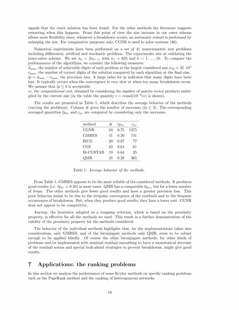
Numerical experiments have been performed on a set of 41 nonsymmetric test problemsincluding differential, artificial and stochastic problems. The experiments aim at validating theinner-outer scheme. We set nk = 2nk−1, with n1 = 625 and k = 1, . . . , 10. To compare theperformances of the algorithms, we consider the following measures:dmax, the number of achievable digits of each problem at the largest considered size n10 = 32 ·104

emax, the number of correct digits of the solution computed by each algorithm at the final size.lp = dmax − emax, the precision loss. A large value for lp indicates that many digits have beenlost. It typically occurs when the convergence is very slow or when too many breakdowns occur.We assume that lp ≤ 3 is acceptable.cc, the computational cost, obtained by considering the number of matrix-vector products multi-plied by the current size (in the table the quantity c = round(10−6cc) is shown).

The results are presented in Table 1, which describes the average behavior of the methods(varying the problems). Column # gives the number of successes (lp ≤ 3). The correspondingaveraged quantities lpav and cav are computed by considering only the successes.

method # lpav cav

CGNR 24 0.75 1275

GMRES 41 0.20 741

BiCG 20 0.67 77

CGS 23 0.64 61

Bi-CGSTAB 19 0.64 35

QMR 35 0.28 365

Table 1: Average behavior of the methods.

From Table 1, GMRES appears to be the most reliable of the considered methods. It producesgood results (i.e. lpav = 0.20) in most cases. QMR has a comparable lpav, but for a lower numberof items. The other methods give fewer good results and have a greater precision loss. Thispoor behavior seems to be due to the irregular convergence of the residuals and to the frequentoccurrences of breakdowns. But, when they produce good results, they have a lower cost. CGNRdoes not appear to be competitive.

Anyway, the heuristics adopted as a stopping criterion, which is based on the proximityproperty, is effective for all the methods we used. This result is a further demonstration of thevalidity of the proximity property for the methods considered.

The behavior of the individual methods highlights that, for the implementations taken intoconsideration, only GMRES, and of the biconjugate methods only QMR, seem to be robustenough to be applied blindly. Of course the other biconjugate methods, for other kinds ofproblems and/or implemented with minimal residual smoothing to force a monotonical decreaseof the residual norms and special look-ahead strategies to prevent breakdowns, might give goodresults.

7 Applications: the ranking problems

In this section we analyze the performance of some Krylov methods on specific ranking problemssuch as the PageRank method and the ranking of heterogeneous networks.

18

7.1 The PageRank computation

Link based ranking techniques view the Web as a directed graph (the Web Graph) G = (V,E),where each of the N pages is a node and each hyperlink is an arc. The problem of ranking webpages consists in assigning a rank of importance to every page based only on the link structure ofthe Web and not on the actual contents of the page. The intuition behind the PageRank algorithmis that a page is “important” if it is pointed by other pages which are in turn “important”. Thisdefinition suggests an iterative fixed-point computation for assigning a ranking score to eachpage in the Web. Formally, in the original model [23], the computation of the PageRank vectoris equivalent to the computation of zT = zTP , where P is a row stochastic matrix obtainedfrom the adjacency matrix of the Web graph G. See [22] for a more deep treatment on thecharacteristics of the model.

In [7] it is shown how the eigenproblem can be rewritten as a sparse linear system provingthat the PageRank vector z, can be obtained by solving a sparse linear system.

Once the problem is transformed into a sparse linear system we can apply numerous iterativesolvers comparing them with the Power method commonly used for computing PageRank. Thematrix involved is moreover an M -matrix hence the convergence of stationary methods is alwaysguaranteed. In [7] the most common methods for linear system solution such as Jacobi, Gauss-Seidel and Reverse Gauss-Seidel and the corresponding block methods are tested. These methodshave been combined with reordering techniques for increasing data-locality, sometime reducingalso the spectral radius of the iteration matrices, and hence increasing the rate of convergence ofthese stationary methods. In particular, schemes for reordering the matrix in block triangularform have been investigated and the performance of classical stationary methods has proven tobe highly improved by reordering techniques also when applying the classical Power method. Inparticular, the combination of reordering techniques and iterative (block or scalar) methods forthe solution of linear systems has proved to be very effective leading to a gain up to 90% in timeand to 60% in terms of Mflops.

In [15] the effectiveness of many iterative methods for linear systems on a parallel architecturehave been tested on the PageRank problem, showing also that the convergence is faster than thesimple Power method.

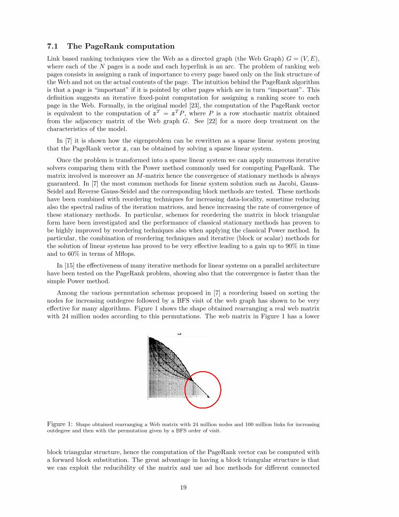
Among the various permutation schemas proposed in [7] a reordering based on sorting thenodes for increasing outdegree followed by a BFS visit of the web graph has shown to be veryeffective for many algorithms. Figure 1 shows the shape obtained rearranging a real web matrixwith 24 million nodes according to this permutations. The web matrix in Figure 1 has a lower

Figure 1: Shape obtained rearranging a Web matrix with 24 million nodes and 100 million links for increasingoutdegree and then with the permutation given by a BFS order of visit.

block triangular structure, hence the computation of the PageRank vector can be computed witha forward block substitution. The great advantage in having a block triangular structure is thatwe can exploit the reducibility of the matrix and use ad hoc methods for different connected

19

components of the matrix. We investigated this idea, using different iterative procedures forsolving the diagonal blocks of the block triangular system. The largest connected componentdiscovered with the BFS order visit of the web graph, is usually huge and for storage constraintswe believe that stationary methods are more adequate because they need just one or two vectorsfor approximating the solution.

The effectiveness of stationary methods is largely discussed in [7] showing that a ReverseGauss-Seidel technique can be very effective. However, for the tail of the matrix, which is thepart circled in Figure 1, we test the effectiveness of different Krylov subspaces iteration methodsversus the classical stationary methods such as Jacobi or Gauss-Seidel algorithms. The idea isthat we use faster methods on smaller problems where memory space is no more a crucial resource.Note that from previous studies [2] it seems that reordering techniques similar to that consideredin this paper can be very effective for improving the convergence of Krylov subspace methodsespecially when used in combination with incomplete factorization preconditioning techniques.

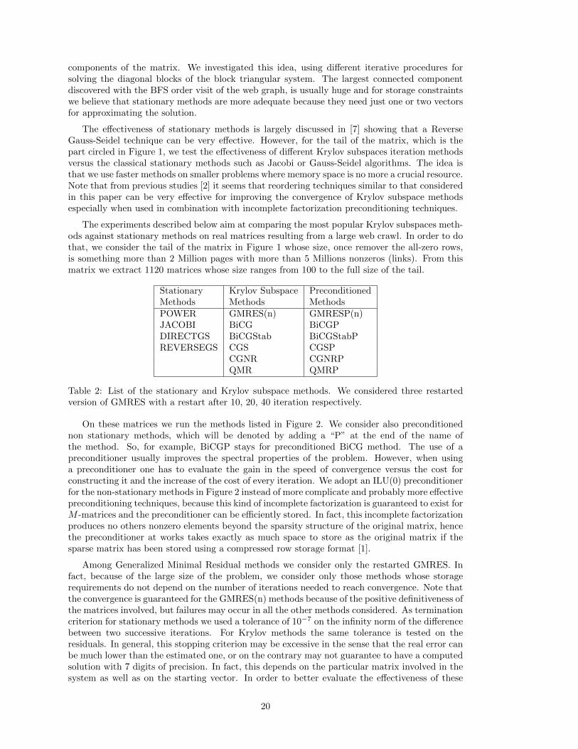
The experiments described below aim at comparing the most popular Krylov subspaces meth-ods against stationary methods on real matrices resulting from a large web crawl. In order to dothat, we consider the tail of the matrix in Figure 1 whose size, once remover the all-zero rows,is something more than 2 Million pages with more than 5 Millions nonzeros (links). From thismatrix we extract 1120 matrices whose size ranges from 100 to the full size of the tail.

Stationary Krylov Subspace PreconditionedMethods Methods MethodsPOWER GMRES(n) GMRESP(n)JACOBI BiCG BiCGPDIRECTGS BiCGStab BiCGStabPREVERSEGS CGS CGSP

CGNR CGNRPQMR QMRP

Table 2: List of the stationary and Krylov subspace methods. We considered three restartedversion of GMRES with a restart after 10, 20, 40 iteration respectively.

On these matrices we run the methods listed in Figure 2. We consider also preconditionednon stationary methods, which will be denoted by adding a “P” at the end of the name ofthe method. So, for example, BiCGP stays for preconditioned BiCG method. The use of apreconditioner usually improves the spectral properties of the problem. However, when usinga preconditioner one has to evaluate the gain in the speed of convergence versus the cost forconstructing it and the increase of the cost of every iteration. We adopt an ILU(0) preconditionerfor the non-stationary methods in Figure 2 instead of more complicate and probably more effectivepreconditioning techniques, because this kind of incomplete factorization is guaranteed to exist forM -matrices and the preconditioner can be efficiently stored. In fact, this incomplete factorizationproduces no others nonzero elements beyond the sparsity structure of the original matrix, hencethe preconditioner at works takes exactly as much space to store as the original matrix if thesparse matrix has been stored using a compressed row storage format [1].

Among Generalized Minimal Residual methods we consider only the restarted GMRES. Infact, because of the large size of the problem, we consider only those methods whose storagerequirements do not depend on the number of iterations needed to reach convergence. Note thatthe convergence is guaranteed for the GMRES(n) methods because of the positive definitiveness ofthe matrices involved, but failures may occur in all the other methods considered. As terminationcriterion for stationary methods we used a tolerance of 10−7 on the infinity norm of the differencebetween two successive iterations. For Krylov methods the same tolerance is tested on theresiduals. In general, this stopping criterion may be excessive in the sense that the real error canbe much lower than the estimated one, or on the contrary may not guarantee to have a computedsolution with 7 digits of precision. In fact, this depends on the particular matrix involved in thesystem as well as on the starting vector. In order to better evaluate the effectiveness of these

20

Methods α = 0.5 α = 0.75 α = 0.85 α = 0.95 α = 0.98

POWER 100 100 100 100 100JACOBI 100 100 100 100 99.7DIRECTGS 100 100 100 100 99.9REVERSEGS 100 100 100 100 100BiCG/BiCGP 42.3/100 10.4/99.5 5.9/98 5.7/87.6 5.6/78BiCGstab/BiCGstabP 99.1/100 80/100 61.2/100 37.8/100 24.0/100CGS/CGSP 59.8/100 25.9/100 7.0/99.3 3.1/92.3 2.9/82.1CGNR/CGNRP 100/100 83.3/99 45.0/96 23.5/65.3 22.5/65.2QMR/QMRP 97.4/100 93.2/99.9 88.9 /99.5 72.4/94.4 63.6/85.4GMRES(10)/GMRESP(10) 100/100 100/100 100/100 94.6/100 66.7/100GMRES(20)/GMRESP(20) 100/100 100/100 100/100 100/100 100/100GMRES(40)/GMRESP(40) 100/100 100/100 100/100 100 /100 100/100

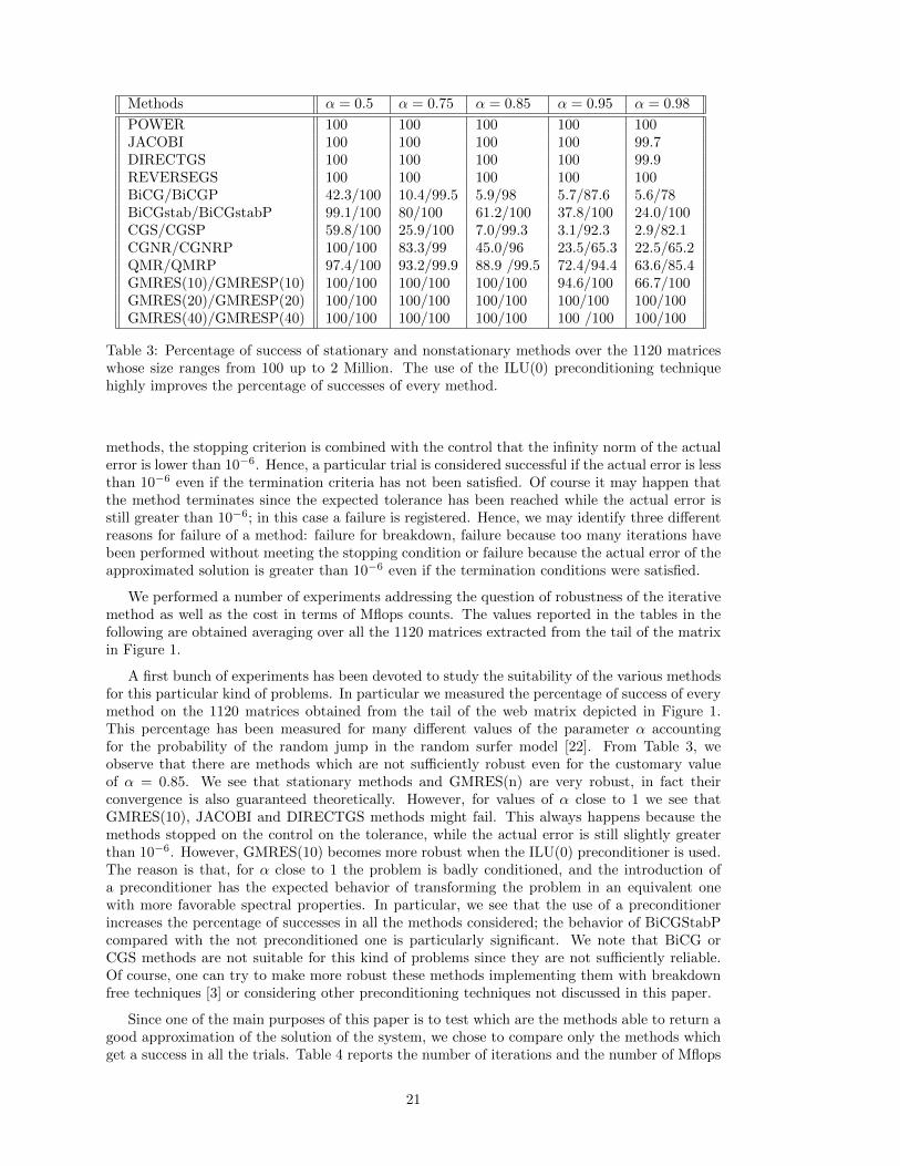
Table 3: Percentage of success of stationary and nonstationary methods over the 1120 matriceswhose size ranges from 100 up to 2 Million. The use of the ILU(0) preconditioning techniquehighly improves the percentage of successes of every method.

methods, the stopping criterion is combined with the control that the infinity norm of the actualerror is lower than 10−6. Hence, a particular trial is considered successful if the actual error is lessthan 10−6 even if the termination criteria has not been satisfied. Of course it may happen thatthe method terminates since the expected tolerance has been reached while the actual error isstill greater than 10−6; in this case a failure is registered. Hence, we may identify three differentreasons for failure of a method: failure for breakdown, failure because too many iterations havebeen performed without meeting the stopping condition or failure because the actual error of theapproximated solution is greater than 10−6 even if the termination conditions were satisfied.

We performed a number of experiments addressing the question of robustness of the iterativemethod as well as the cost in terms of Mflops counts. The values reported in the tables in thefollowing are obtained averaging over all the 1120 matrices extracted from the tail of the matrixin Figure 1.

A first bunch of experiments has been devoted to study the suitability of the various methodsfor this particular kind of problems. In particular we measured the percentage of success of everymethod on the 1120 matrices obtained from the tail of the web matrix depicted in Figure 1.This percentage has been measured for many different values of the parameter α accountingfor the probability of the random jump in the random surfer model [22]. From Table 3, weobserve that there are methods which are not sufficiently robust even for the customary valueof α = 0.85. We see that stationary methods and GMRES(n) are very robust, in fact theirconvergence is also guaranteed theoretically. However, for values of α close to 1 we see thatGMRES(10), JACOBI and DIRECTGS methods might fail. This always happens because themethods stopped on the control on the tolerance, while the actual error is still slightly greaterthan 10−6. However, GMRES(10) becomes more robust when the ILU(0) preconditioner is used.The reason is that, for α close to 1 the problem is badly conditioned, and the introduction ofa preconditioner has the expected behavior of transforming the problem in an equivalent onewith more favorable spectral properties. In particular, we see that the use of a preconditionerincreases the percentage of successes in all the methods considered; the behavior of BiCGStabPcompared with the not preconditioned one is particularly significant. We note that BiCG orCGS methods are not suitable for this kind of problems since they are not sufficiently reliable.Of course, one can try to make more robust these methods implementing them with breakdownfree techniques [3] or considering other preconditioning techniques not discussed in this paper.

Since one of the main purposes of this paper is to test which are the methods able to return agood approximation of the solution of the system, we chose to compare only the methods whichget a success in all the trials. Table 4 reports the number of iterations and the number of Mflops

21

Methods α = 0.5 α = 0.75 α = 0.85 α = 0.95 α = 0.98

POWER 32.05 9.82 73.28 23.01 125.47 41.03 370.97 127.59 807.40 247.64REVERSEGS 15.80 2.94 34.65 6.27 58.53 10.67 170.92 31.52 407.44 75.50BCGSTABP 4.00 5.27 7.08 9.25 9.67 13.24 16.64 23.79 24.68 37.13GMRES10P 8.80 7.08 14.50 12.43 19.47 17.76 34.57 36.51 54.82 66.88GMRES20 21.04 15.67 35.88 33.57 48.76 53.28 90.06 143.13 155.74 336.16GMRES20P 8.79 7.37 14.02 15.67 18.46 21.85 30.73 43.07 45.83 73.94GMRES40 20.77 21.59 33.97 50.15 44.54 81.70 72.15 205.90 105.58 465.92GMRES40P 8.79 7.37 14.01 16.85 18.20 28.68 28.89 57.82 41.01 94.77

Table 4: For every method and for different values of α we report the mean number of iterationsand the mean number of Mflops needed to meet the stopping criterion of 10−7. These valueshave been obtained averaging over the 1120 matrices of different size. For every value of α inboldface we highlight the best value in terms of average number of iterations and Mflops

50 100 150 200 250 300 350IT

10

20

30

40

50

Mflop

BiCGStabP

REVERSEGS

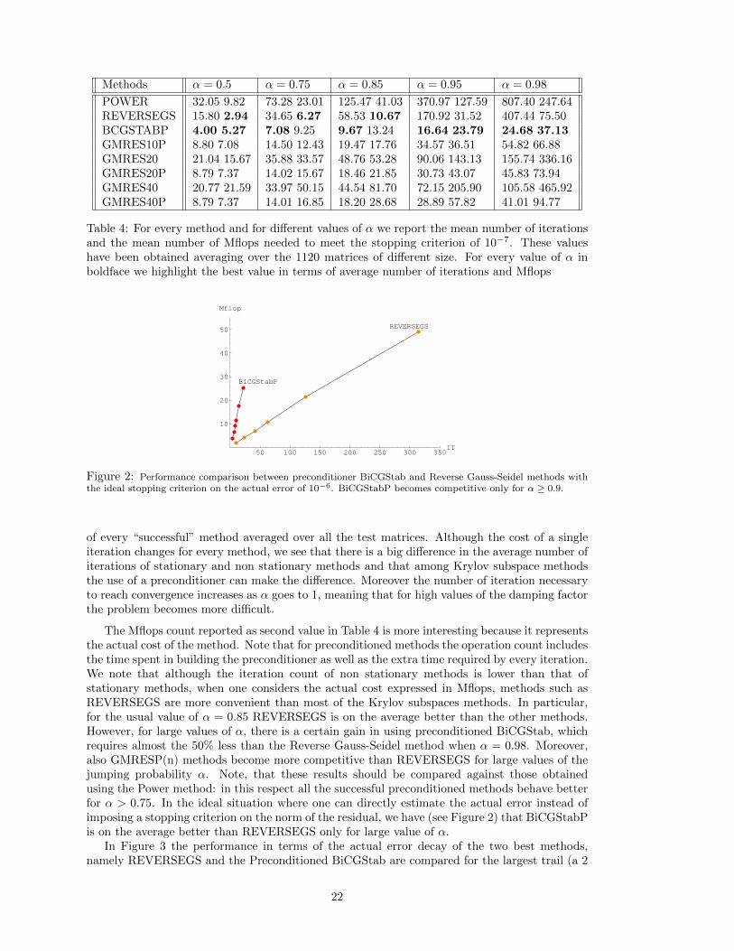
Figure 2: Performance comparison between preconditioner BiCGStab and Reverse Gauss-Seidel methods withthe ideal stopping criterion on the actual error of 10−6. BiCGStabP becomes competitive only for α ≥ 0.9.

of every “successful” method averaged over all the test matrices. Although the cost of a singleiteration changes for every method, we see that there is a big difference in the average number ofiterations of stationary and non stationary methods and that among Krylov subspace methodsthe use of a preconditioner can make the difference. Moreover the number of iteration necessaryto reach convergence increases as α goes to 1, meaning that for high values of the damping factorthe problem becomes more difficult.

The Mflops count reported as second value in Table 4 is more interesting because it representsthe actual cost of the method. Note that for preconditioned methods the operation count includesthe time spent in building the preconditioner as well as the extra time required by every iteration.We note that although the iteration count of non stationary methods is lower than that ofstationary methods, when one considers the actual cost expressed in Mflops, methods such asREVERSEGS are more convenient than most of the Krylov subspaces methods. In particular,for the usual value of α = 0.85 REVERSEGS is on the average better than the other methods.However, for large values of α, there is a certain gain in using preconditioned BiCGStab, whichrequires almost the 50% less than the Reverse Gauss-Seidel method when α = 0.98. Moreover,also GMRESP(n) methods become more competitive than REVERSEGS for large values of thejumping probability α. Note, that these results should be compared against those obtainedusing the Power method: in this respect all the successful preconditioned methods behave betterfor α > 0.75. In the ideal situation where one can directly estimate the actual error instead ofimposing a stopping criterion on the norm of the residual, we have (see Figure 2) that BiCGStabPis on the average better than REVERSEGS only for large value of α.

In Figure 3 the performance in terms of the actual error decay of the two best methods,namely REVERSEGS and the Preconditioned BiCGStab are compared for the largest trail (a 2

22

10 20 30 40 50 60It

-5

-4

-3

-2

-1

0Log Err

BiCGstabReverse GS

500 1000 1500 2000 2500Mflop

-5

-4

-3

-2

-1

0Log Err

BiCGstab

Reverse GS

Figure 3: Comparison between the best two methods on the largest trail with α = 0.85. In the first graphic itis plotted the behavior of the error as a function of the number of iterations. In the second graphic the error isplotted as a function of the Mflops.

Million size matrix) for α = 0.85. In the first figure we show the decay of the error as a functionof the number of iterations. We note that BiCGStab does not show a monotony decay while astheoretically predicted we have a linear decay for REVERSEGS. In the second part of Figure 3the error is plotted as a function of the number of operations necessary expressed in Mflops. Wesee that computationally REVERSEGS is more convenient than Krylov stationary methods forlarge matrices and values of α not too close to 1.

7.2 Ranking of heterogeneous networks

An heterogeneous network is described by a directed graph G = (V,E) and two mapping func-tions, one for the nodes τ : V → A and one for the edges φ : E → R. Each node v ∈ V belongs toa particular type τ(v) ∈ A and each edge e ∈ E belongs to a particular type of relation φ(e) ∈ R.Functions φ and τ are such that if e1 and e2 are two edges, e1 = (v1, v2) and e2 = (w1, w2), withφ(e1) = φ(e2), then τ(v1) = τ(w1) and τ(v2) = τ(w2). When |A| > 1 and |R| > 1 we say thatthe graph is a multigraph.

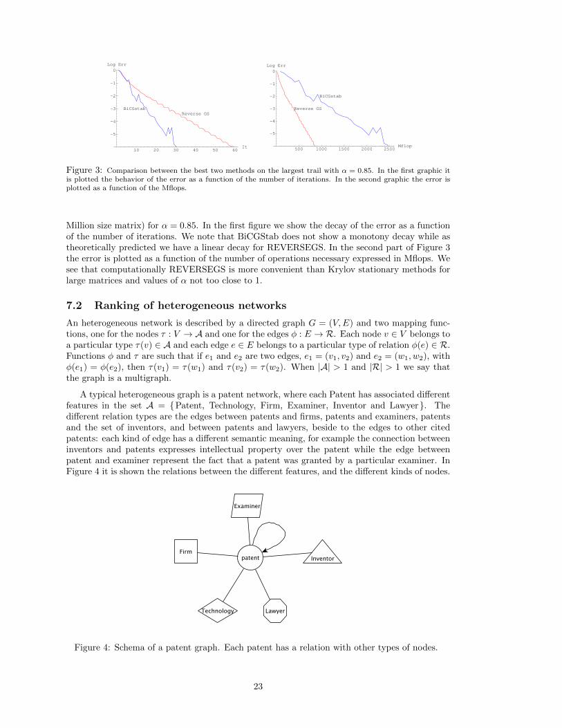
A typical heterogeneous graph is a patent network, where each Patent has associated differentfeatures in the set A = {Patent, Technology, Firm, Examiner, Inventor and Lawyer}. Thedifferent relation types are the edges between patents and firms, patents and examiners, patentsand the set of inventors, and between patents and lawyers, beside to the edges to other citedpatents: each kind of edge has a different semantic meaning, for example the connection betweeninventors and patents expresses intellectual property over the patent while the edge betweenpatent and examiner represent the fact that a patent was granted by a particular examiner. InFigure 4 it is shown the relations between the different features, and the different kinds of nodes.

Figure 4: Schema of a patent graph. Each patent has a relation with other types of nodes.

23

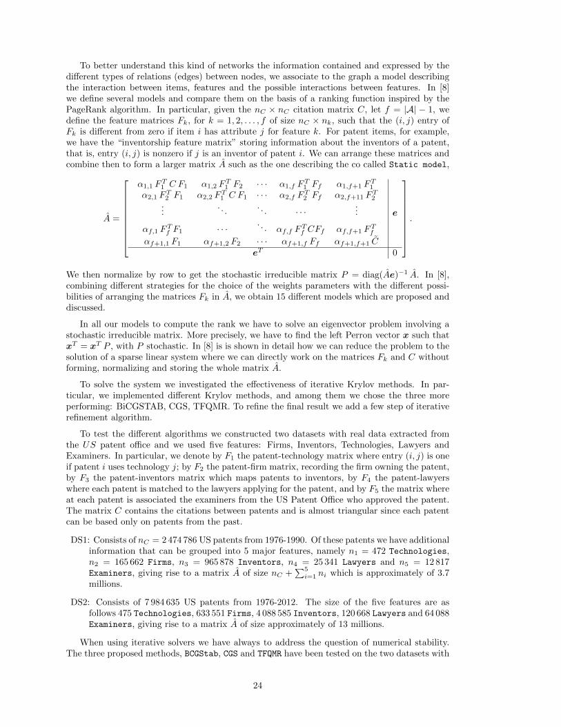
To better understand this kind of networks the information contained and expressed by thedifferent types of relations (edges) between nodes, we associate to the graph a model describingthe interaction between items, features and the possible interactions between features. In [8]we define several models and compare them on the basis of a ranking function inspired by thePageRank algorithm. In particular, given the nC × nC citation matrix C, let f = |A| − 1, wedefine the feature matrices Fk, for k = 1, 2, . . . , f of size nC × nk, such that the (i, j) entry ofFk is different from zero if item i has attribute j for feature k. For patent items, for example,we have the “inventorship feature matrix” storing information about the inventors of a patent,that is, entry (i, j) is nonzero if j is an inventor of patent i. We can arrange these matrices andcombine then to form a larger matrix A such as the one describing the co called Static model,

A =

α1,1 FT1 C F1 α1,2 F

T1 F2 · · · α1,f F

T1 Ff α1,f+1 F

T1

α2,1 FT2 F1 α2,2 F

T1 C F1 · · · α2,f F

T2 Ff α2,f+11 F

T2

.... . .

. . . · · ·...

αf,1 FTf F1 · · ·

. . . αf,f FTf CFf αf,f+1 F

Tf

αf+1,1 F1 αf+1,2 F2 · · · αf+1,f Ff αf+1,f+1 C

e

eT 0

.

We then normalize by row to get the stochastic irreducible matrix P = diag(Ae)−1 A. In [8],combining different strategies for the choice of the weights parameters with the different possi-bilities of arranging the matrices Fk in A, we obtain 15 different models which are proposed anddiscussed.

In all our models to compute the rank we have to solve an eigenvector problem involving astochastic irreducible matrix. More precisely, we have to find the left Perron vector x such thatxT = xT P , with P stochastic. In [8] is is shown in detail how we can reduce the problem to thesolution of a sparse linear system where we can directly work on the matrices Fk and C withoutforming, normalizing and storing the whole matrix A.

To solve the system we investigated the effectiveness of iterative Krylov methods. In par-ticular, we implemented different Krylov methods, and among them we chose the three moreperforming: BiCGSTAB, CGS, TFQMR. To refine the final result we add a few step of iterativerefinement algorithm.

To test the different algorithms we constructed two datasets with real data extracted fromthe US patent office and we used five features: Firms, Inventors, Technologies, Lawyers andExaminers. In particular, we denote by F1 the patent-technology matrix where entry (i, j) is oneif patent i uses technology j; by F2 the patent-firm matrix, recording the firm owning the patent,by F3 the patent-inventors matrix which maps patents to inventors, by F4 the patent-lawyerswhere each patent is matched to the lawyers applying for the patent, and by F5 the matrix whereat each patent is associated the examiners from the US Patent Office who approved the patent.The matrix C contains the citations between patents and is almost triangular since each patentcan be based only on patents from the past.

DS1: Consists of nC = 2 474 786 US patents from 1976-1990. Of these patents we have additionalinformation that can be grouped into 5 major features, namely n1 = 472 Technologies,n2 = 165 662 Firms, n3 = 965 878 Inventors, n4 = 25 341 Lawyers and n5 = 12 817Examiners, giving rise to a matrix A of size nC +

∑5i=1 ni which is approximately of 3.7

millions.

DS2: Consists of 7 984 635 US patents from 1976-2012. The size of the five features are asfollows 475 Technologies, 633 551 Firms, 4 088 585 Inventors, 120 668 Lawyers and 64 088Examiners, giving rise to a matrix A of size approximately of 13 millions.

When using iterative solvers we have always to address the question of numerical stability.The three proposed methods, BCGStab, CGS and TFQMR have been tested on the two datasets with

24

models BCGstab CGS TFQMR

it log10(res) it log10(res) it log10(res)

Stiff-U 18 -10.49 100 -7.71 21 -3.90Stiff-D 23 -11.77 100 -11.20 19 -4.75Static-U 35 -9.03 100 -6.25 40 -7.83Static-D 39 -11.13 100 -7.22 37 -9.60Static-DD 35 -12.33 100 -12.20 30 -11.99Heap-U 32 -9.86 100 -7.44 36 -8.59Heap-D 36 -11.26 100 -7.73 38 -9.74Heap-DD 41 -11.48 100 -9.46 33 -11.51Heap-H 36 -10.83 100 -6.46 30 -7.72Heap-HH 24 -9.85 100 -7.14 27 -8.38SHeap-U 32 -11.56 100 -8.00 29 -9.91SHeap-D 32 -11.72 100 -8.51 28 -9.85SHeap-DD 37 -11.43 100 -11.83 28 -11.97SHeap-H 28 -10.56 100 -8.33 25 -9.98SHeap-HH 29 -11.34 100 -6.75 24 -10.05

Table 5: Performance comparison between three Krylov methods on the 15 models on a problemof size 3.7 million.

models BCGstab TFQMR

it log10(res) it log10(res)

Stiff-U 14 -10.57 19 -3.83Stiff-D 21 -11.30 25 -3.71Static-U 37 -6.77 52 -3.09Static-D 52 -10.53 53 -7.89Static-DD 39 -11.38 43 -8.70Heap-U 36 -8.87 47 -7.58Heap-D 45 -6.47 51 -6.11Heap-DD 41 -9.40 41 -6.56Heap-H 40 -9.63 43 -7.31Heap-HH 35 -9.49 43 -7.52SHeap-U 40 -9.78 38 -7.48SHeap-D 38 -10.36 36 -8.10SHeap-DD 36 -11.75 34 -9.79SHeap-H 31 -7.90 35 -4.54SHeap-HH 35 -10.63 35 -5.91

Table 6: Performance comparison between two Krylov methods applied to the 15 models on theproblem of size 13 million.

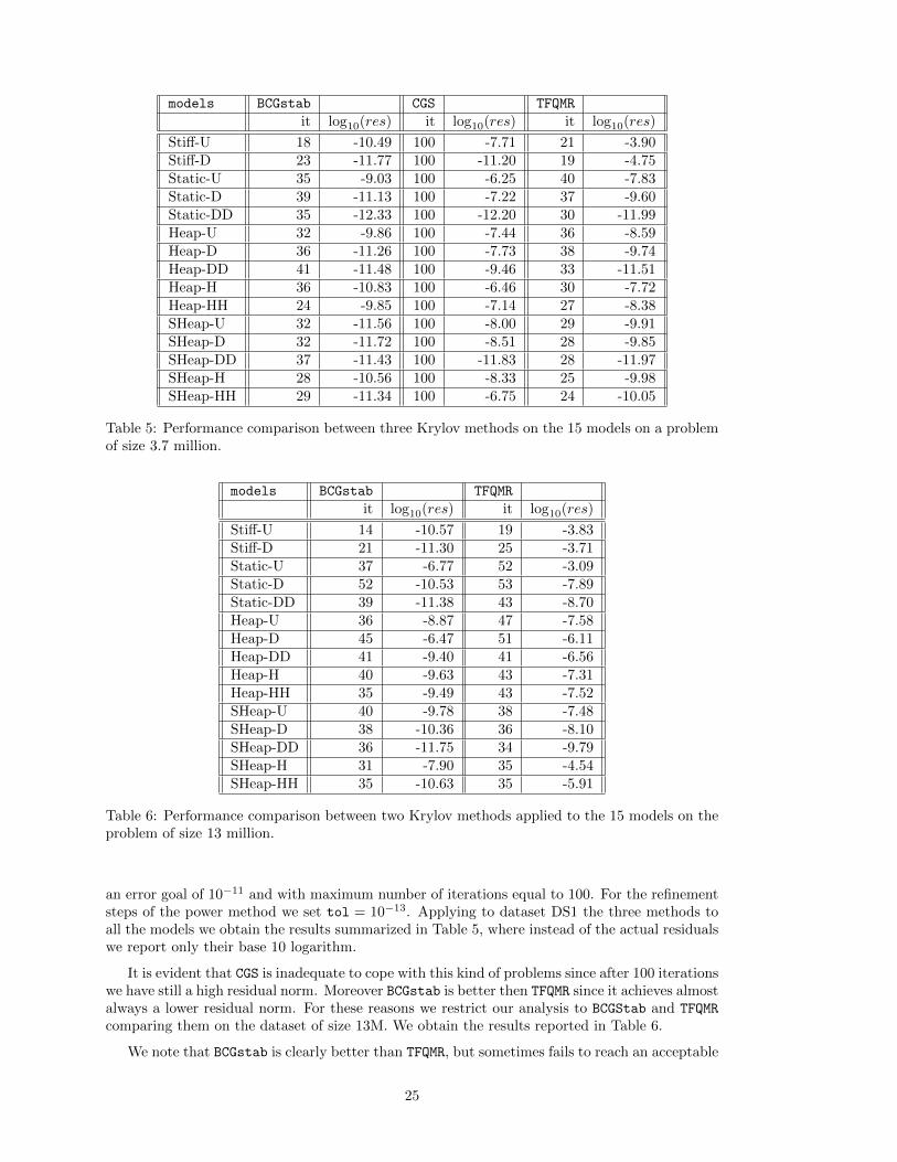
an error goal of 10−11 and with maximum number of iterations equal to 100. For the refinementsteps of the power method we set tol = 10−13. Applying to dataset DS1 the three methods toall the models we obtain the results summarized in Table 5, where instead of the actual residualswe report only their base 10 logarithm.

It is evident that CGS is inadequate to cope with this kind of problems since after 100 iterationswe have still a high residual norm. Moreover BCGstab is better then TFQMR since it achieves almostalways a lower residual norm. For these reasons we restrict our analysis to BCGStab and TFQMR

comparing them on the dataset of size 13M. We obtain the results reported in Table 6.

We note that BCGstab is clearly better than TFQMR, but sometimes fails to reach an acceptable

25

models DS1 size=3.7M DS2 size =13Mtime(sec.) log10(res) time(sec.) log10(res)

Stiff-U 237 -12.095 1078 -11.952Stiff-D 179 -12.762 1422 -12.1884

Static-U (*)239 -10.536 (*)2314 -9.0309Static-D 188 -11.740 2096 -10.536Static-DD 161 -13.002 1688 -11.7138

Heap-U 509 -11.138 (*)5992 -9.7579Heap-D 467 -11.740 (*)7509 -10.536Heap-DD 450 -12.535 (*)5849 -11.6019Heap-H 440 -11.138 (*)5978 -9.93399Heap-HH (*)403 -11.439 (*)4999 -10.235

SHeap-U 80 -11.740 (*)717 -11.1381SHeap-D 70 -11.439 661 -11.4391SHeap-DD 67 -13.107 604 -12.3703SHeap-H 86 -12.041 (*)662 -10.8371SHeap-HH 60 -11.689 595 -10.536

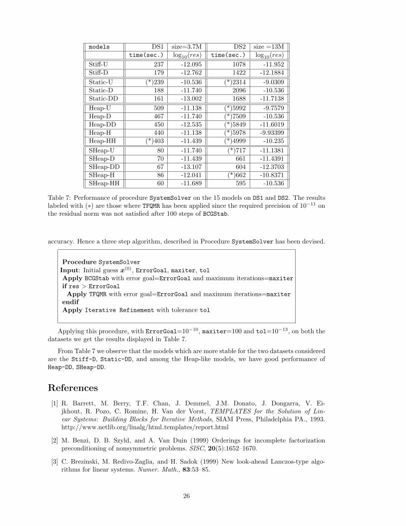
Table 7: Performance of procedure SystemSolver on the 15 models on DS1 and DS2. The resultslabeled with (∗) are those where TFQMR has been applied since the required precision of 10−11 onthe residual norm was not satisfied after 100 steps of BCGStab.

accuracy. Hence a three step algorithm, described in Procedure SystemSolver has been devised.

Procedure SystemSolver

Input: Initial guess x(0), ErrorGoal, maxiter, tolApply BCGStab with error goal=ErrorGoal and maximum iterations=maxiter

if res > ErrorGoal

Apply TFQMR with error goal=ErrorGoal and maximum iterations=maxiter

endifApply Iterative Refinement with tolerance tol

Applying this procedure, with ErrorGoal=10−10, maxiter=100 and tol=10−13, on both thedatasets we get the results displayed in Table 7.

From Table 7 we observe that the models which are more stable for the two datasets consideredare the Stiff-D, Static-DD, and among the Heap-like models, we have good performance ofHeap-DD, SHeap-DD.

References

[1] R. Barrett, M. Berry, T.F. Chan, J. Demmel, J.M. Donato, J. Dongarra, V. Ei-jkhout, R. Pozo, C. Romine, H. Van der Vorst, TEMPLATES for the Solution of Lin-ear Systems: Building Blocks for Iterative Methods, SIAM Press, Philadelphia PA., 1993.http://www.netlib.org/linalg/html templates/report.html

[2] M. Benzi, D. B. Szyld, and A. Van Duin (1999) Orderings for incomplete factorizationpreconditioning of nonsymmetric problems. SISC, 20(5):1652–1670.

[3] C. Brezinski, M. Redivo-Zaglia, and H. Sadok (1999) New look-ahead Lanczos-type algo-rithms for linear systems. Numer. Math., 83:53–85.

26

[4] P. Brianzi, P. Favati, O. Menchi, F. Romani (2006) A framework for studying the regularizingproperties of Krylov subspace methods, Inverse Problems, 22, 1007–1021.

[5] D. Calvetti, B. Lewis and L. Reichel (2002) On the regularizing properties of the GMRESmethod Numer. Math. 91, 605–625.

[6] D. Calvetti, B. Lewis and L. Reichel (2002) Krylov subspaces iterative methods for non-symmetric discrete ill-posed problems in image restoration Proc. Society of Photo-OpticalInstrumentation Engineers (SPIE) vol. 4474 (Bellingham, WA: The International Societyfor Optical Engineering) 224–33.

[7] G. M. Del Corso, A. Gullı, and F. Romani (2005) Fast PageRank computation via a sparselinear system. Internet Mathematics, 2(3), 251–273.

[8] G. M. Del Corso and F. Romani (2015) A multi-class approach for ranking graph nodes:models and experiments with incomplete data. arXiv:1504.07766.

[9] J. Dongarra and F. Sullivan. (2000) Guest editor: introduction to the top 10 algorithmsComputing in Science and Engineering, 2(1), 22–23.

[10] P. Favati, G. Lotti, O. Menchi, F. Romani (2007) Adaptive solution of infinite linear systemsby Krylov subspace methods, Journal of Computational and Applied Mathematics, 210, 191-199.

[11] P. Favati, G. Lotti, O. Menchi, F. Romani (2014) Generalized Cross-Validation applied toConjugate Gradient for discrete ill-posed problems, Applied Mathematics and Computation,243, 258–268.

[12] P. Favati, G. Lotti, O. Menchi, F. Romani (2014) An inner-outer regularizing method forill-posed problems, Inverse Problems and Imaging, 8, 409–420.

[13] R.W. Freund and N.M. Nachtigal (1991) QMR: a quasi-minimal residual method for non-Hermitian linear systems. Numer. Math., 60, 315–339.

[14] R.W. Freund, G.H.Golub and N.M. Nachtigal (1992) Iterative solution of linear systemsActa Numerica, 57–100.

[15] D. Gleich, L. Zhukov, and P. Berkhin (2004) Fast parallel PageRank: A linear systemapproach. Technical Report Yahoo!.

[16] M.H. Gutknecht (2005) A brief introduction to Krylov space methods for solving linearsystems, Frontiers of Computational Science – Proceedings of the International Symposiumon Frontiers of Computational Science (Y. Kaneda, H. Kawamura, and M. Sasai, eds.),53–62, Springer-Verlag, Berlin Heidelberg.

[17] P.C. Hansen (1994) Regularization tools: a Matlab package for analysis and solution ofdiscrete ill-posed problems Numerical Algorithms 6 1–35.

[18] P.C.Hansen (1998) Rank-Deficient and Discrete Ill-Posed Problems (Philadelphia: SIAMMonographs on Mathematical Modeling and Computation)

[19] R. Hestenes and E. Stiefel (1952) Methods of conjugate gradients for solving linear systemsJ. Res. Nat. Bureau Standards, 49, 409–435.

[20] A.N. Krylov. On the numerical solution of the equation by which in technical ques-tions frequencies of small oscillations of material systems are determined (in Russian).Izvestija AN SSSR (News of Academy of Sciences of the USSR), Otdel. mat. i estest. nauk,1931, VII, Nr.4, 491–539, cited by M. Botchev (2002) “A.N. Krylov, a short biography”http://www.staff.science.uu.nl/ vorst102/kryl.html

27

[21] C. Lanczos (1952) Solution of systems of linear equations by minimized iterations. J. Res.Nat. Bureau Standards, 49, 33–53.

[22] A. N. Langville and C. D. Meyer (2005) A survey of eigenvector methods of Web informationretrieval. SIAM Review, 47, 135–161.

[23] L. Page, S. Brin, R. Motwani, and T. Winograd (1998) The PageRank citation ranking:Bringing order to the Web. Technical report, Stanford.

[24] C. C. Paige and M. A. Saunders (1975) Solution of sparse indefinite systems of linear equa-tionsSIAM J. Numer. Anal., 12, 617–629.

[25] R. Plato (1990) Optimal algorithms for linear ill-posed problems yield regularization methodsNum. Funct. Anal. and Optimiz. 11, 111–118

[26] Y. Saad and M. H. Schultz (1985) Conjugate gradient-like algorithms for solving nonsym-metric linear systems. Math. Comp., 44, 417–424.

[27] Y. Saad (1996) Iterative methods for sparse linear systems. PWS Publishing Company,Boston.

[28] P. Sonneveld (1989) CGS, a fast Lanczos-type solver for nonsymmetric linear systems SIAMJ. Sci. Statist. Comput., 10, 36–52.

[29] H. A. van der Vorst (1992) Bi-CGSTAB: a fast and smoothly converging variant of BiCG forthe solution of nonsymmetric linear systems SIAM J. Sci. Statist. Comput., 13, 631–644.

28