Title:

Krylov subspace methods for computing hydrodynamic interactions in Brownian dynamics

simulations

By Tadashi Ando, Edmond Chow, Yousef Saad and Jeffrey Skolnick

Author affiliations:

Tadashi Ando

Center for the Study of Systems Biology, School of Biology, Georgia Institute of Technology,

250 14th Street NW, Atlanta, GA 30318-5304

Edmond Chow

School of Computational Science and Engineering, College of Computing, Georgia Institute

of Technology, 266 Ferst Drive, Atlanta, GA 30332-0765

Yousef Saad

Department of Computer Science and Engineering, University of Minnesota, 200 Union

Street SE, Minneapolis, MN 55455

1

Jeffrey Skolnick

Center for the Study of Systems Biology, School of Biology, Georgia Institute of Technology,

250 14th Street NW, Atlanta, GA 30318-5304

2

Abstract

Hydrodynamic interactions play an important role in the dynamics of macromolecules. The

most common way to take into account hydrodynamic effects in molecular simulations is in

the context of a Brownian dynamics simulation. However, the calculation of correlated

Brownian noise vectors in these simulations is computationally very demanding and

alternative methods are desirable. This paper studies methods based on Krylov subspaces for

computing Brownian noise vectors. These methods are related to Chebyshev polynomial

approximations, but do not require eigenvalue estimates. We show that only low accuracy is

required in the Brownian noise vectors to accurately compute values of dynamic and static

properties of polymer and monodisperse suspension models. With this level of accuracy, the

computational time of Krylov subspace methods scales very nearly as O(N2) for the number

of particles N up to 10,000, which was the limit tested. The performance of the Krylov

subspace methods, especially the “block” version, is slightly better than that of the

Chebyshev method, even without taking into account the additional cost of eigenvalue

estimates required by the latter. Furthermore, at N = 10,000, the Krylov subspace method is

13 times faster than the exact Cholesky method. Thus, Krylov subspace methods are

recommended for performing large-scale Brownian dynamics simulations with hydrodynamic

interactions.

3

I. INTRODUCTION

Brownian dynamics (BD) is a computational technique for simulating the motion of

macromolecules in a fluid environment.1 Globular molecules such as proteins may be treated

as coarse-grained particles, possibly of different sizes, while polymers such as DNA/RNA or

proteins may be treated, for example, by a bead-spring model. Interactions between particles

(or beads) with the solvent are modeled by random forces corresponding to particle collisions

with solvent molecules, as well as a Stokes drag force proportional to particle velocity.

The solvent also mediates interactions between the particles themselves. This gives

rise to so-called hydrodynamic interactions (HI), where the motion of one particle through the

fluid induces a force on all the other particles. If one is only interested in equilibrium

thermodynamic properties, HI do not play any role and can be neglected.1 On the other hand,

it is essential to include HI to correctly capture the dynamics of colloidal spheres,

macromolecules, and swimming bacteria at a low Reynolds number; in particular, their

collective, intermolecular motions can give rise to qualitatively different dynamic behavior.2-4

Hydrodynamic interactions are modeled by a configuration-dependent diffusion

matrix, D, of size 3N × 3N for a system of N particles. This matrix is dense, owing to the

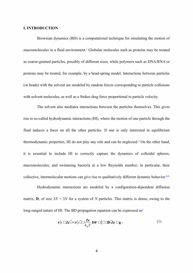
long-ranged nature of HI. The BD propagation equation can be expressed as1

( ) ( ) ( ) gDDFrr +∆⋅∇+∆+=∆+ tTk

tttt

B

, (1)

4

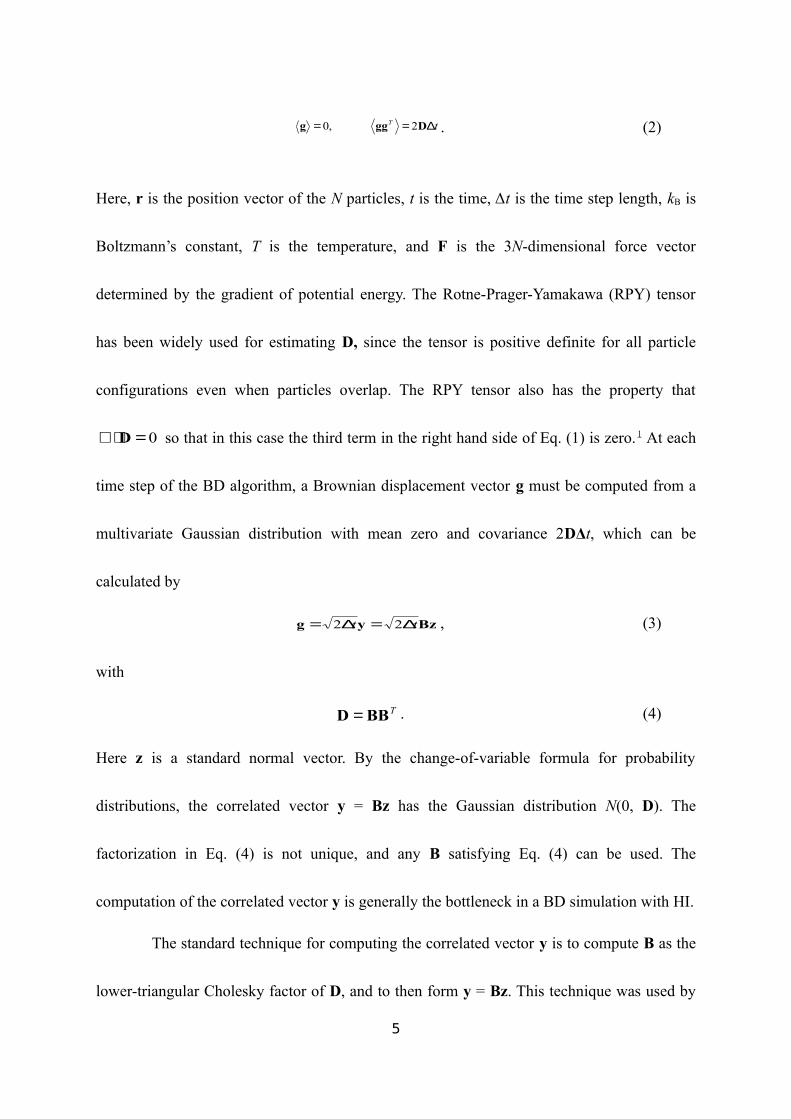
tT ∆== Dggg 2,0 . (2)

Here, r is the position vector of the N particles, t is the time, Δt is the time step length, kB is

Boltzmann’s constant, T is the temperature, and F is the 3N-dimensional force vector

determined by the gradient of potential energy. The Rotne-Prager-Yamakawa (RPY) tensor

has been widely used for estimating D, since the tensor is positive definite for all particle

configurations even when particles overlap. The RPY tensor also has the property that

0=⋅∇ D so that in this case the third term in the right hand side of Eq. (1) is zero. 1 At each

time step of the BD algorithm, a Brownian displacement vector g must be computed from a

multivariate Gaussian distribution with mean zero and covariance 2DΔt, which can be

calculated by

Bzyg tt ∆=∆= 22 , (3)

with

TBBD = . (4)

Here z is a standard normal vector. By the change-of-variable formula for probability

distributions, the correlated vector y = Bz has the Gaussian distribution N(0, D). The

factorization in Eq. (4) is not unique, and any B satisfying Eq. (4) can be used. The

computation of the correlated vector y is generally the bottleneck in a BD simulation with HI.

The standard technique for computing the correlated vector y is to compute B as the

lower-triangular Cholesky factor of D, and to then form y = Bz. This technique was used by

5

Ermak and McCammon in their original BD algorithm.1 The cost of computing the Cholesky

factorization is O(N3), although this cost in practice can be amortized over many time steps if

D changes slowly.

The other major technique used in BD with HI is the Chebyshev polynomial

approximation proposed by Fixman.7 In this approximation technique, an approximate

correlated vector is computed as p(D)z, where p(D) is a polynomial in D that approximates

the principal square root of D. This square root corresponds to the factorization in Eq. (4)

where B = BT. The technique is based on Chebyshev polynomials and requires estimates of

the extreme eigenvalues of D. The matrix p(D) itself is not necessary and is never formed

explicitly, and thus O(N3) matrix-matrix multiplications are avoided. The arithmetic

complexity is observed to grow as O(N2.25).

Recently, a new method called the truncated expansion approximation (TEA) was

proposed for calculating correlated vectors in BD.11 TEA assumes a particular form for these

correlated vectors and is particularly effective in cases where the correlations among all

particles are approximately equal and relatively weak. This method has spurred much

interest, attesting to the growing importance of fast methods for computing HI.12 TEA has

been found to work efficiently for bead-spring random polymers. However, when multiple

beads are assembled into compact structures, the TEA method does not show the correct

scaling of translational diffusivity with N.14

6

In this paper, we study Krylov subspace methods for computing correlated Brownian

displacements for use in BD. The methods are not new in the numerical analysis

community,15-17 but to the best of our knowledge, they appear to be unknown in the BD

literature. These methods have two major advantages over Chebyshev polynomial

approximations. First, estimates of the extreme eigenvalues of D, required in the Chebyshev

approximation, are not required in Krylov subspace methods. This is a great simplification

over Chebyshev approximations. Second, block versions of Krylov subspace methods

converge faster than Chebyshev approximations, and therefore require fewer computations

for the same level of accuracy. Block versions of Krylov subspace methods are applicable

when D changes slowly and can be reused for several consecutive time steps. Finally, in this

paper, we also study the accuracy required by Krylov subspace methods in BD simulations.

This is done for three different simulation models.

II. THEORY

A. Chebyshev Polynomial Approximations

The principal square root of a symmetric, positive definite matrix D may be

approximated by a polynomial, p(D), where p(λ) is small, when λ is an eigenvalue of D.

Fixman7 proposed an approximation to the Brownian correlated vector y ≈ p(D)z based on

Chebyshev polynomials. Such polynomial approximations of the square root of a matrix

7

times a vector (and in general, any function of a matrix times a vector) appeared soon

afterward in the numerical analysis literature,15-17 but these studies were unaware of Fixman's

contribution. An essential feature of these approximations is that p(D) is not needed and is

never computed explicitly; rather, only p(D)z is required, which can be computed much more

efficiently.

Chebyshev polynomials have the property that they are small in the interval [−1, 1].

To approximate f(D), where the function f in our case is the square root, and where the

spectrum of D lies in the interval [a, b], we approximate instead the function g(Ds), where

IDDab

ba

ab −+−

−= 2

s , (5)

which has eigenvalues in the interval [−1, 1]. The function g is then defined as

( )

++−= IDD

22 ss

baabfg (6)

where I in the above expressions denotes the identity matrix. In other words, we use

Chebyshev polynomials to approximate g(Ds), which is equal to f(D). Thus, the extreme

eigenvalues of D are required to perform the above change of variables. The more accurate

the estimates of these extreme eigenvalues, the faster is the convergence. Convergence can be

very poor if any eigenvalue of D lies outside these estimates. (The convergence rate is the

inverse of the degree of the polynomial required for a given level of accuracy.)

Beginning with Fixman, procedures have been developed for estimating the extreme

8

eigenvalues of D and also for updating these estimates as a BD simulation progresses. The

updates may be performed dynamically, according to measures of the accuracy of the

Chebyshev approximation. A recent comparison of these techniques found that the run time

may differ significantly with different approaches.13 As shown below, Krylov subspace

approximations employed in this paper do not require eigenvalue estimates.

The Chebyshev polynomial expansion up to degree L is

( ) ( )∑=

+=L

kkkL Tc

cp

1s

0s 2

DD , (7)

where ck denotes the expansion coefficients and Tk denotes the k-th Chebyshev polynomial.

The expansion coefficients are computed by interpolating the function g at L+1 points,

generally selected to be the Chebyshev nodes. Due to the discrete orthogonality property of

Chebyshev polynomials, the coefficients are easily computed.

B. Truncated Expansion Approximation

In the truncated expansion approximation (TEA) proposed by Geyer and Winter,11 the

correlated vector y is assumed to be of a specific form (an ansatz), namely y = STEAz, where

( ) ( )( ) 211TEA dd DDBDCS ⋅= − , (8)

where Dd is the matrix that is the diagonal part of D, the matrix B has diagonal entries 1 and

off-diagonal entries β, the “dot” operator represents an element-wise product, and C is a

9

diagonal matrix. TEA chooses the entries in C and the value of β so that

DSS ≈TTEATEA , (9)

which is the requirement that y approximately has covariance D. The value of β is chosen

based on the assumption that the off-diagonal couplings in D are small relative to the

diagonal of D; specifically, they are chosen by replacing the off-diagonal entries in D by their

average value. The entries in C are chosen such that the diagonal of STEASTEAT matches the

diagonal of D. The overall procedure is O(N2). The computational cost of the method is

somewhat more than that of three matrix-vector products with D: computing the entries in C,

computing β, and multiplying by D.

Details of this method are available elsewhere.11 What we have presented here is an

algebraic description of the method. The method has been shown to be very efficient and

effective, in particular, for bead-spring chain models.

C. Krylov Subspace Approximation

We now present Krylov subspace approximations for computing the correlated

vector y. Consider first the exact computation of y via the principal square root of D, which is

given by

zUUΛzD y T2121 == , (10)

where Λ is the 3N × 3N diagonal matrix whose elements are the eigenvalues of D, and U is

the 3N × 3N matrix whose columns are eigenvectors of D. Computing the correlated vector

10

directly this way requires an eigenvalue decomposition of D, which is O(N3) computations

and not any better than using the Cholesky factorization approach.

In the Krylov subspace approach, instead of the exact method, an approximation y~

to D1/2z is constructed from the Krylov subspace

( ) { }zDDzzzD 1,,,span, −= mmK , (11)

where m ≤ 3N. The approximation y~ can be observed to be a linear combination of vectors

of the form Diz, with 0 ≤ i ≤ m−1, and thus, such an approximation has the form pm−1(D)z,

where pm−1 is a polynomial of degree m−1 or less. Krylov subspace approximations are thus a

form of polynomial approximation. Like the Chebyshev approximation, the coefficients of

this polynomial are chosen by interpolating the square root function, although implicitly and

at different points than those used by the Chebyshev method.17 Thus, we expect Krylov

subspace approximations and Chebyshev polynomial approximations of similar degree to

have similar quality, although Krylov subspace approximations may be somewhat more

efficient because pm−1(λ) is designed to be small when λ is an eigenvalue of D, rather than

uniformly small over the entire interval from the smallest to largest eigenvalues of D, as in

the Chebyshev case.

An important advantage of the Krylov subspace approximation approach over the

Chebyshev approach is that estimates of the spectrum of D are not necessary.

Since D is symmetric, the Lanczos process can be used for constructing an

11

orthonormal basis for the Krylov subspace. The approximation y~ is then constructed in this

basis. Let a 3N × m matrix Vm = [v1, v2, …, vm] be an orthonormal basis for the Krylov

subspace. The optimal approximation, one that minimizes the 2-norm of the error from this

subspace, is

zDVVy 21* Tmm= , (12)

which is the orthogonal projection of the exact solution onto the Krylov subspace. Let us now

choose the basis Vm such that the first vector of this basis is v1 = z/||z||2. Here ||z||2 is the 2-

norm of vector z, which is the square root of the sum of squares of the entries of the vector.

Thus, z = ||z||2Vme1 with e1 being the first column of the m × m identity matrix. Then we can

write the optimal approximation as

121

2* eVDVVzy m

Tmm= . (13)

Now, we define the symmetric tridiagonal matrix mTmm DVVH = , which is automatically

calculated in the Lanczos process as shown below. After the matrix Hm is obtained, one can

easily compute its eigenvalue decomposition when m << 3N:

Tmmmm PΣPH = . (14)

Here Σm is the m × m diagonal matrix whose diagonal elements are eigenvalues of Hm and Pm

is the m × m matrix whose columns are eigenvectors of Hm. The eigenvalues of Hm are known

to approximate the extremal eigenvalues of D, and VmPm are the corresponding

12

approximations to the eigenvectors. Therefore, we approximate mTm VDV 21 as

( )( ) ( )

.21

21

21

2121

m

Tmmm

mT

mmmmmTm

mTT

mmTm

H

PΣP

VPVΣPVV

VUUΛVVDV

=

=

≈

=

(15)

Here, we used IVV =mTm . Thus, an approximation for Eq. (13) can be written as

121

2~ eHVzy mm≈ . (16)

The approximation is thus based on computing the matrix square root on a much smaller

subspace, where it is inexpensive to compute exactly, and then mapping the result to the

original space. Note that like the Chebyshev polynomial approximation, an approximation to

D1/2 is never computed explicitly.

1. Lanczos Process

The matrix D is symmetric and thus an orthonormal basis Vm for the Krylov

subspace can be computed using the Lanczos process. The matrix Hm is computed

automatically in this method. This is the same process used in the Lanczos method for

solving symmetric eigen-problems, where the spectrum of Hm approximates the spectrum of

D. The overall algorithm for computing the approximate correlated vector y~ with Gaussian

distribution N(0, D) is shown in Algorithm 1. In the algorithm, m is the number of Lanczos

steps.

13

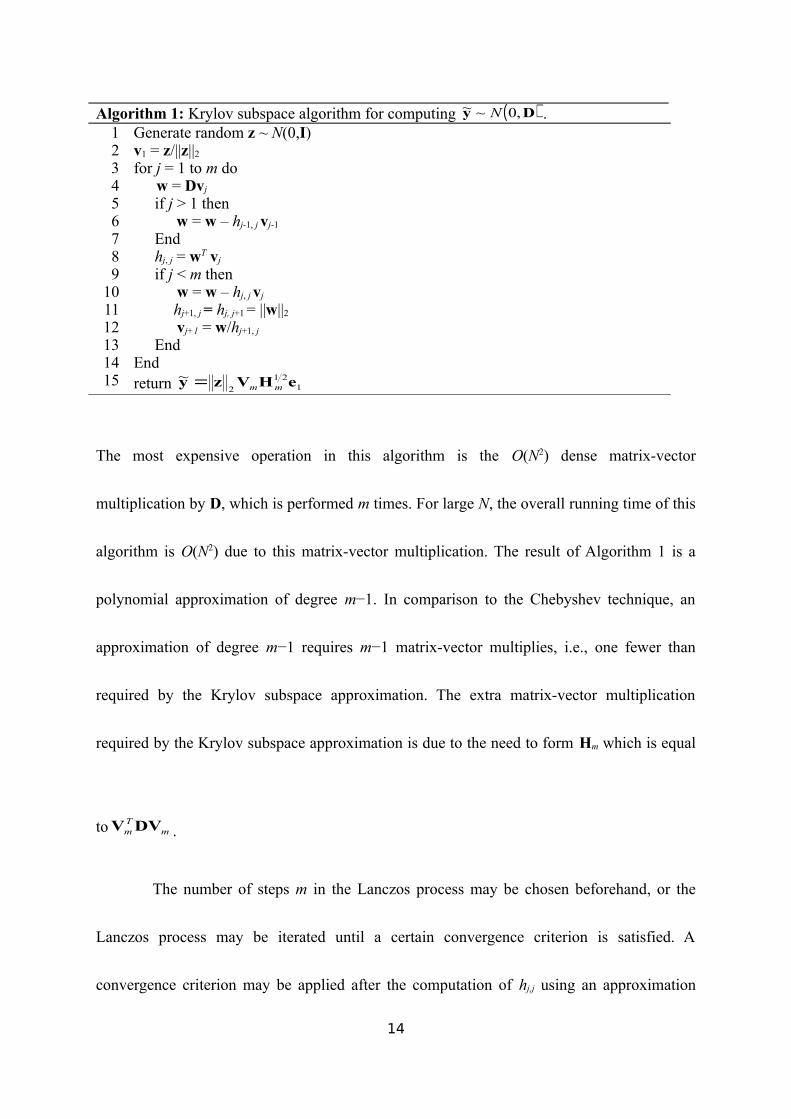
Algorithm 1: Krylov subspace algorithm for computing ( )Dy ,0~~ N .1 Generate random z ~ N(0,I)2 v1 = z/||z||23 for j = 1 to m do4 w = Dvj

5 if j > 1 then6 w = w – hj-1, j vj-1

7 End8 hj, j = wT vj

9 if j < m then10 w = w – hj, j vj

11 hj+1, j = hj, j+1 = ||w||212 vj+1 = w/hj+1, j

13 End14 End15 return 1

21

2~ eHVzy mm=

The most expensive operation in this algorithm is the O(N2) dense matrix-vector

multiplication by D, which is performed m times. For large N, the overall running time of this

algorithm is O(N2) due to this matrix-vector multiplication. The result of Algorithm 1 is a

polynomial approximation of degree m−1. In comparison to the Chebyshev technique, an

approximation of degree m−1 requires m−1 matrix-vector multiplies, i.e., one fewer than

required by the Krylov subspace approximation. The extra matrix-vector multiplication

required by the Krylov subspace approximation is due to the need to form Hm which is equal

to mTm DVV .

The number of steps m in the Lanczos process may be chosen beforehand, or the

Lanczos process may be iterated until a certain convergence criterion is satisfied. A

convergence criterion may be applied after the computation of hj,j using an approximation

14

ky~ computed at each Lanczos step, and using the basis vectors computed thus far. This

approximation is used in the convergence criterion to be described later.

2. Block-Lanczos Process for Multiple Vectors

In BD simulations, the covariance matrix generally changes slowly, making it possible to use

the same covariance matrix for several time steps. When the Cholesky factorization approach

is used, this avoids the need to compute the factorization at every time step. For further

computational efficiency, the correlated vectors for several time steps should be computed

simultaneously, as one block of vectors, rather than one vector at a time. The multiplication of

the Cholesky factor by a block of standard normal vectors should be carried out such that all

the multiplications are performed while traversing the elements of the Cholesky factor only

once. This reduces data movement which has relatively high cost compared to arithmetic

computations on modern processors.20 If the Chebyshev polynomial approach is used, it is

likewise advantageous to compute multiple vectors simultaneously because of the efficiency

of computing matrix-vector products with a block of vectors.

For the Lanczos approach, a block variant can also be used when multiple sample

vectors can be computed for the same covariance matrix. Like the above, computational

efficiency is gained by operating on a block of vectors simultaneously. However, there is an

additional important advantage: the solution for each vector can be sought in a larger

15

subspace (larger than in the single-vector case) for very little additional cost. Thus the

solutions converge much more quickly and require fewer matrix-vector multiplications in

total.

Consider the block-Lanczos process for a block of s independent standard normal

vectors, z1, …, zs. After m steps, the block-Lanczos process computes an orthonormal basis

Vms for the combined subspaces

( ) ( )smm KK zDzD ,, 1 ++ . (17)

Each step of the algorithm produces s basis vectors, one vector for each of the subspaces in

the “sum” above. The block-Lanczos process also computes the ms × ms banded matrix

msTmsms DVVH = .

Let Z = [z1, …, zs] denote a block of s standard normal vectors. Let Vj denote the j-th

block of s vectors computed and available at the beginning of step j of the block-Lanczos

process. An approximation to a block of correlated vectors with covariance D in the space

spanned by Vms is given by

ZDVVY 21* Tmsms= . (18)

Let Z = QR be the reduced QR factorization of Z and choose V1 = Q. Then

16

[ ]

=

0121* R

VVDVVY mTmsms , (19)

where the quantity in square brackets is Vms and where R is s × s. As in the single-vector case,

we now make the approximation

=

0~ 21 R

HVY msms. (20)

This procedure is embodied in the algorithm below. We use Hi,j to denote the (i, j) block (of

size s × s) of matrix Hms. Like Algorithm 1, the cost of the algorithm is dominated by the

matrix-vector multiplication by D.

Algorithm 2: Block-Krylov subspace algorithm for computing a block of s correlated

vectors, Y~ , each vector with distribution ( )D,0N .1 Generate a block of s vectors Z, each vector with distribution N(0,I)2 Compute reduced QR factorization V1R = Z3 for j = 1 to m do4 W = DVj

5 if j > 1 then

17

6 W = W –Vj-1Hj-1, j

7 end8 Hj, j = Vj

T W9 if j < m then

10 W = W –Vj Hj, j

11 Compute reduced QR factorization Vj+1Hj+1,j = W12 Hj, j+1 = Hj+1, j

13 end14 end15

return

=

0~ 21 R

HVY msms

III. MODELS AND SIMULATION METHODS

A. Random polymer chain model

Random polymer bead-spring models have been widely used not only for theoretical studies

of hydrodynamic interactions but also for evaluating simulation accuracy. The polymer

consists of N beads of radius a, each connected to their first neighbors by harmonic springs

with potential

( ) 2ss 2

2

1axkV −= . (21)

Here, ks is the spring constant and x is the distance between the beads. To prevent bead

overlap, a repulsive harmonic potential between beads i and j with | i – j | ≥ 2 is applied:

18

( )

≥

<−=

,2for 0

,2for 22

1 2r

r

ax

axaxkV (22)

where kr is the force constant. In this study, ks = kr = 125 kBT/a2 was used. Polymers with N =

10, 20, 40, 60, 80, 100, 200 were examined in BD simulations. For timing tests and to study

convergence of the Krylov subspace methods, we used much longer polymers. Five

independent initial configurations were generated for each chain length, where beads were

randomly placed without significant overlaps under the constraint of distances between beads

i and i+1 of 2a. These configurations were then subjected to short-time energy minimization.

This model does not have any attractive interactions between beads and thus corresponds to a

polymer in a good solvent.23

B. Collapsed chain model

For many applications of BD, especially for biological simulations, attractive interactions are

applied to particles or beads to analyze the dynamics of self-organization of molecules and

molecular associations.24-26 Therefore, testing a model with attractive interactions is quite

important. Here, we examine a simple chain model that collapses to a compact conformation.

This model corresponds to a polymer in a poor solvent.23

Adjacent beads are connected by the harmonic springs described by Eq. (21).

19

Between beads i and j with |i – j| ≥ 2, a Lennard-Jones 12-6 potential is applied:

−

=

6

LJ

12

LJLJLJ 2

xxV

σσε , (23)

where εLJ is the energy depth and σLJ is the distance at the energy minimum. In this study, εLJ

= 1 kBT and σLJ = 2a were used. Polymers of length N = 10, 20, 40, 60, 80, 100, 200 were

considered in BD simulations. Completely extended configurations were used as initial states

and five independent BD simulations were performed with different random number seeds.

To further study the convergence of the Krylov subspace methods, we used long polymers

with N = 1,000. For these long polymers, initial configurations were generated by the same

procedure as in the random polymer model, and then BD simulations with HI were performed

to obtain equilibrated states.

C. Monodisperse suspension model

Another model we used for evaluating simulation accuracy is a monodisperse suspension of

N particles of radius a. To help prevent bead overlap, a repulsive harmonic potential between

particles as described by Eq. (22) was used. Five different volume fractions Φ of 0.1, 0.2, 0.3,

0.4, and 0.5 were considered in periodic boxes. A value of N of 200 was used in BD

simulations. For convergence tests, N of 1,000 was also examined. Five independent initial

configurations were generated for each condition, where particles were randomly placed

20

without significant overlaps in simulation boxes and subjected to short-time energy

minimization. As described in the next section, we use the RPY tensor to account for HI in

the BD simulations. The RPY tensor represents only the far-field part of HI and the tensor is

not appropriate by itself for simulations at high volume fractions. For simulations at high

volume fractions, a more sophisticated formulation that also incorporates near-field HI is

necessary. In these formulations, the RPY tensor corresponding to high volume fraction is

utilized to represent the far-field part of HI (technically, it is the inverse of this RPY tensor

that is the far-field component of the covariance matrix).

D. Brownian dynamics simulation and analysis

The integration algorithm for BD described in Eq. (1) was used. In this work, we employ the

RPY tensor for estimating D:

( )

<≠

+

−

≥≠

−++

=

=

.2,ˆˆ32

3

32

91

6

,2,ˆˆ3

12ˆˆ

8

,6

B

2

2B

B

arjia

r

a

r

a

Tk

arjir

a

r

Tk

jia

Tk

ijijijijij

ijijij

ij

ijijij

ij

rrI

rrIrrI

I

D

π η

π η

π η

(24)

where i and j are the indices of particles, rij is ri – rj, rij is the length of rij, ijijij rrr =ˆ , and I is

the unit tensor. For periodic boundary conditions, since HI have a long-range nature similar to

21

electrostatic interactions, an Ewald summation of the RPY tensor to obtain D of the system is

necessary not only for accuracy but also for giving a positive definite matrix D. We used the

Ewald sum technique originally derived by Beenakker29 and modified by Zhou and Chen30 to

allow for particle overlap.

For the sake of simplicity, all quantities are expressed in dimensionless units. Length

is in units of the bead radii, a, and time is units of a2/D0, where D0 = kBT/6πηa is the diffusion

coefficient of a single bead in dilute solution. Simulations were performed for 5.0 × 10 6 steps

with a time step Δt of 0.002 for the random polymer chain and monodisperse suspension

models. For the following analysis of the random polymer and monodisperse suspension

models, the first 5.0 × 105 steps were discarded. For the collapsed chain model, at least 4.0 ×

106 steps were run after the chains collapsed into their compact structures with Δt of 0.001 in

the presence of HI and Δt of 0.0005 in the absence of HI.

Translational diffusion coefficients of the centers of masses, Dcm, were estimated by

( ) ( )( )2cmcmcm6 ttD rr −+= ττ , (25)

where the brackets indicate an average over configurations separated by a time difference τ

and rcm is the center of mass of the polymer. Translational diffusion coefficients of particles,

D, were calculated by the same equation where rcm is replaced by the position, ri, of particle i,

and the brackets indicate an average over configurations separated by a time difference τ and

over all particles.

22

IV. RESULTS AND DISCUSSION

A. Convergence

1. Convergence rate and error estimates

The Krylov subspace method iteratively improves the accuracy of the approximate correlated

vector. An estimate of the error of this correlated vector is desired. We define the relative

norm of the exact error of the k-th approximation as

2

212

21

exact

~

zD

zDy −=

k

kE , (26)

where z is the same standard normal vector used to compute y~ . This of course cannot be

computed in practice. We propose an approximation based on two consecutive iterates

21

21

~

~~

−

−−=

k

kkkE

y

yy. (27)

This estimate is natural when convergence is monotonic, which is generally the case. The

estimate is particularly good if convergence is rapid. In Figure 1A, convergence of the Krylov

method measured by Ekexact and Ek for a random polymer with N = 1,000 is shown as a

representative example. (In this and later figures, the iteration count on the x-axis is equal to

the polynomial degree less one of the Krylov subspace or Chebyshev approximation.) We

observe that Ek closely follows Ekexact. This result indicates that Ek may be used for monitoring

convergence in real simulations. We thus propose using Ek as the convergence criterion of the

23

Krylov subspace methods. When the estimate falls below a user-supplied threshold, then

convergence is assumed and the iterations are stopped.

Jendrejack et al.8 proposed the following quantity for monitoring the convergence of

the Chebyshev method,

Dzz

DzzyyT

TT

fE−

=~~

. (28)

If zDy 21~ = exactly, then Ef = 0. When Ef is large, then y~ is inaccurate. The quantity Ef can

thus be used to adaptively control the Chebyshev polynomial approximation as a simulation

progresses. For example, when Ef is large, this may indicate that the eigenvalue estimates are

no longer accurate and/or that the polynomial degree is not large enough. The extreme

eigenvalues are then recomputed and/or the polynomial degree is then adjusted and the

current time step is repeated. A threshold of 10−3 has been suggested to indicate sufficient

accuracy, although no strong justification has been given.

The quantity Ef, however, turns out to be inappropriate for monitoring the Krylov

subspace approximation, as this approximation always produces a result such that Ef = 0. This

is because the iterates produced by Krylov subspace methods are already scaled such that Ef =

0. To see this, we form

24

( )

( )

.

~~

11

2

2

11

2

2

11

2

2

12121

1

2

2

Dzz

Dvvz

eDVVez

eHez

eHVVHezyy

T

T

mTm

T

mT

mmTm

T

mTT

=

=

≈

=

=

(29)

In general, a small value of Ef does not always imply that y~ is accurate; any y~ can be

“improved” by a scaling so that Ef = 0.

It is also possible for the Chebyshev approximation to use the error estimate Eq.

(27). In this case, ky~ and 1~

−ky correspond to the degree k and degree k−1 polynomial

approximations, respectively. Convergence of the Chebyshev method as measured by Ekexact,

Ek, and Ef for the random polymer with N = 1,000 is shown in Figure 1B. We observe again

that Ek closely tracks Ekexact, suggesting that Ek may be useful for estimating the accuracy of

the Chebyshev approximation. The quantity Ef, on the other hand, does not appear monotonic

although the exact error decreases monotonically.

Comparing Figures 1A and 1B, we observe that the convergence rate of the Krylov

subspace approximation is somewhat faster than that of the Chebyshev polynomial

approximation.

2. Effect of block size on convergence

In Figure 2A, the effect of block size on the convergence of the block-Krylov method is

shown for the random polymer model with N = 1,000. The convergence rate increases with

25

block size as expected. The Ekexact and Ek estimates (for the first vector of the block of vectors)

during the block-Krylov iteration are shown in Figure 2B. We observe that Ek tracks Ekexact,

indicating that Ek would be again useful for checking convergence in practice.

Another effect of the block size is the improved computational performance when

matrix-vector products are performed with a block of vectors simultaneously, compared to

performing multiple matrix-vector products with single vectors. We will study this

computational efficiency of the block-Krylov method in Section IV-C.

3. Simulation model properties affecting convergence

Differences in convergence between the random and collapsed polymer models, and between

N = 200 and 1,000 are compared in Figure 3A. Convergence is slower for larger N and for

collapsed polymers. In Figure 3B, the dependence of convergence rate on volume fraction for

the monodisperse suspension model with N = 200 and 1,000 are shown. Slower convergence

for the higher volume fractions and the larger systems is observed. If convergence rates in the

Krylov subspace methods are strongly dependent on N, the algorithmic scaling is larger than

O(N2). However, the convergence is insensitive to N in the Krylov methods when Ek < ~0.01,

as seen later in Figure 7. Therefore, we might expect near O(N2) scaling for the Krylov

methods if low accuracy of Brownian noise vectors are sufficient for BD simulations. We will

discuss the accuracy of Brownian noise vectors and the scaling of the Krylov subspace

26

methods in the following sections.

B. BD simulations

In this section, we perform BD simulations with the three different models using Krylov

subspace methods and check if dynamic properties of the model systems obtained from the

simulations reproduce the results using the standard Cholesky factorization method.

Statistical errors in the translational diffusion coefficients Dcm and D are less than 5% on

average. We also evaluated the radius of gyration, Rg, as a static polymer property.

Conclusions obtained from analysis of Rg are essentially the same as those for Dcm. Therefore,

we show results only on Dcm for the polymer models in this text.

1. Update interval of diffusion tensor

In BD simulations, the diffusion matrix changes slowly, making it possible to use the same

matrix for several time steps, significantly reducing computational cost. This also allows us

to use block versions of Krylov subspace methods. In this section, we determine an

appropriate update interval, λRPY, for the RPY diffusion matrix in BD simulations. We use the

Cholesky factorization for computing correlated vectors in order to not confound these results

with further approximations.

Figure 4A shows a log-log plot of Dcm as a function of length N for random polymers

obtained from BD simulation using various values of λRPY. Theoretical scaling for this

27

property is ν−∝ NDcm . In a good solvent and in the presence of HI, as N → ∞, the scaling

exponent has a theoretical value of ν ≈ 0.588 from a perturbation analysis.31 Our simulation of

the random polymer model using λRPY = 1 gives ν = 0.57 for Dcm in the presence of HI, in

good agreement with the prediction. BD simulations with λRPY = 25 – 200 also provide Dcm of

random polymers close to those obtained from the simulation with λRPY = 1 for all chain

lengths examined in this study. For all conditions with λRPY = 25 – 200, the relative error is

less than 2% for Dcm. Even if λRPY = 800 was used, the error was less than 4%. These results

indicate that the random polymer model is quite insensitive to the update interval of the RPY

tensor.

Effects of λRPY on Dcm for the collapsed chain model are also shown in Figure 4A.

This model corresponds to polymers in poor solvent, where the scaling exponent of ν = 0.33

is predicted.23 BD simulations with λRPY = 1 provide ν = 0.35 for Dcm, which is also good

agreement with theory. Like the above, the relative errors in Dcm are small for all λRPY

conditions. The collapsed polymer model is thus also quite insensitive to the update interval

of the RPY tensor.

The diffusion coefficients of particles, D, obtained from BD simulations in a

monodisperse suspension at various volume fractions with various λRPY are shown in Figure

4B. Errors in D obtained with various λRPY relative to values of D with λRPY = 1 are listed in

Table I. In contrast to the single chain polymer models, D values are significantly affected by

28

λRPY in the monodisperse suspension model. With λRPY = 200, the errors are more than 10% at

volume fractions of 0.4 and 0.5, which exceeds the statistical error in our analysis. The errors

in the results with λRPY = 100 are less than 10% for all volume fractions. However, at

moderate to high volume fractions (Φ = 0.3 – 0.5), the errors are slightly higher than those at

low volume fractions but are still greater than 5%. With λRPY = 25 and 50, the errors are less

than 5% for all volume fractions. Compared with the polymer models, particles in the

monodisperse suspension model can move easily due to the lack of harmonic constraints. In

addition, attractive interactions between beads in the collapsed polymer model restrict the

motions of beads. Therefore, the diffusion tensor of the monodisperse suspension model may

change more rapidly than in the single chain polymer models.

2. Required accuracy of Brownian noise vectors

In this section, we study the accuracy of the correlated Brownian noise vectors required for

accurate simulation results. The use of an appropriate level of accuracy is critical for

obtaining maximum efficiency of approximate methods such as the Krylov subspace and

Chebyshev methods. We used the Krylov subspace method to generate correlated Brownian

noise vectors with accuracy controlled by values of Ek of 0.1, 0.01, and 0.001. The choice of

λRPY = 50 was adopted which was shown in the previous section to give results comparable to

those of λRPY = 1 for all models. We also performed BD simulations using the TEA method

29

for comparison.

The accuracy of Dcm for the random polymer chain model obtained from BD

simulations using the Krylov subspace method with various Ek as well as using the TEA

method are listed in Table II. All values of Ek examined here for the Krylov subspace method

matched the Cholesky results with relative errors in Dcm of less than 4%. The TEA method

results are within the average error of 8%, consistent with the results reported by Geyer and

Winter.11 Values of Rg obtained from BD simulations with the Krylov subspace method and

TEA were also close to the Cholesky results (data not shown).

Since the collapsed polymers are packed into compact structures, small noise in

Brownian noise vectors may cause significant clashes between beads. Therefore, the model

would be sensitive to the accuracy of correlated Brownian noise vectors. Errors in Dcm of the

collapsed polymer chains obtained from the BD simulations using the Krylov method with

various values of Ek as well as using the TEA method are listed in Table III. The results of the

Krylov method with Ek of 0.001 – 0.1 have a relative error less than 5%. For TEA, errors in

Dcm are about −16%, for all chain lengths. Geyer also reported the low estimation of Dcm by

the TEA method for spherical objects consisting of many small particles.14

We also evaluated the relaxation time τcorr for the autocorrelation function

ree t( ) ⋅ree 0( ) of the end-to-end vector ree for the polymer models, which may be sensitive

to the accuracy of Brownian noise vectors. Although the values of relaxation times obtained

30

from the BD simulations have large noise due to limited simulation length, the Krylov

subspace method even with Ek = 0.1 gave close values to the Cholesky results and qualitative

differences between them were not observed (data not shown). We also studied polymers

modeled using a finite extensible nonlinear elastic (FENE) potential with a soft-core

repulsive potential function. We performed the same analysis as above with this polymer

model and obtained the same conclusions (data not shown).

Diffusion coefficients of particles in the monodisperse suspension system at various

volume fractions obtained from the BD simulation using the Krylov subspace method with

various Ek as well as using the TEA method are listed in Table IV. For the monodisperse

suspension model, diffusivities of particles obtained from the Krylov subspace method with

three different Ek are within a 5% error for all volume fractions. On the other hand, results at

high volume fractions obtained by the TEA method significantly deviate from the Cholesky

results (27~50%). This defect in TEA is not surprising since an assumption in the TEA

method is that the hydrodynamic coupling is weak; at low volume fractions, this assumption

is correct, but at high volume fractions, the average distances between particles become

small, resulting in strong hydrodynamic coupling.

In this section, we estimated the required accuracy of Brownian noise vectors in the

Krylov subspace method. Results for the three different models show that a value of Ek of 0.1

would be practically adequate and a value of Ek of 0.01 would be sufficient to reproduce the

31

Cholesky results within statistical error. In this study, a λRPY of 50 was used for all models,

where the relative errors in diffusivities of all three models are less than 5%. However, as

shown in Figure 4 and Table I, much larger values of λRPY could be used for polymers at dilute

solution in good and poor solvents, resulting in great saving in computational time without a

significant loss of simulation accuracy.

3. Comparison of covariance matrix generated from Brownian noise vectors

In this section, we seek to understand why low levels of accuracy can be used in Krylov

subspace and Chebyshev polynomial approximations yet computed model properties from a

BD simulation are essentially unaffected.

Given a set of correlated vectors XY~ generated by a method X, its average XY

~

should be ~0 and a covariance matrix CX constructed from XY~ should be close to D,

( ) DCYY ≈= XXX ~,

~cov . (30)

The difference between CX and D can be quantified by the relative error

F

F

X

XED

DC −=1 . (31)

Here, ||·||F is the Frobenius norm, which is defined to be the square root of the sum of the

squares of the entries of a matrix. In this analysis, an identical set of uncorrelated Gaussian

noise vectors is used for all methods as input. The relative error when the Cholesky

32

factorization is used, E1Cholesky, is the lowest value of E1 that can be expected for a given

number of correlated vectors. The values of E1 for the Cholesky, Krylov subspace with Ek =

0.1, and TEA methods as a function of the number of correlated vectors up to 10,000 are

shown in Figure 5. In addition, we observed that E1Krylov with Ek = 0.01 and 0.001 always track

E1Cholesky for all models with N = 200 and 1,000 and they are indistinguishable from each other

for any number of input noise vectors (data not shown). Values of E1Krylov with Ek = 0.1

slightly deviate from E1Cholesky for the collapsed polymer model, although the differences are

smaller than 0.01. The average XY~

for all cases is close to zero (data not shown). We also

did the same analysis for the random polymer N = 10 with up to 107 input noise vectors for Ek

= 0.4, 0.1, and 0.01 to see converged E1 values, showing that E1 converged to 0.08, 0.02, and

0.003, respectively, which are much smaller than their Ek values in input vectors. These

results seem to suggest that using Ek = 0.01 in the Krylov subspace methods would be

sufficient to generate correlated Brownian noise vectors whose accuracy is indistinguishable

from that of the Cholesky method. Even for Ek = 0.1 in the Krylov subspace methods, the

error in the generated covariance matrix would have about 1%, which would be also

sufficient for BD simulations. For Chebyshev, results similar to the Krylov methods are

observed (data not shown).

The values of E1 for TEA are always larger than those of the Cholesky method for

the polymer and monodisperse suspension models. These results indicate that each correlated

33

vector calculated by TEA has small errors and these errors accumulate, resulting in

significant deviation from the exact covariance matrix. Geyer and Winter,11 and Schmidt et

al.13 reported that the TEA method could reproduce Cholesky results for random polymers in

a good solvent and a theta solvent. The polymers in these conditions are not closely packed.

Therefore, since the models may be insensitive to noise in the correlated Brownian vectors,

the TEA method might reproduce the Cholesky results for these models.

C. Computational time

Finally, we evaluate the computational efficiency of the Krylov subspace methods. For the

following timing tests, the random polymer model with N = 1,000 – 10,000 was used. Values

of Ek of 0.1 and 0.01 were used for the stopping criterion. Cholesky, Chebyshev, and TEA

methods are also examined for comparison. These tests were performed on a quad-core AMD

Opteron processor and the algorithms were parallelized by hand. The GOTO BLAS library32

was used for matrix factorization and matrix-matrix and matrix-vector multiplications in the

algorithms. It is important to note that the time for estimating eigenvalues is not included in

the Chebyshev results and the eigenvalues calculated by diagonalization are used in the

method.

For the block-Krylov subspace method, we expect good performance of the

algorithm due to enhanced convergence rate and computational efficiency. The effect of block

34

size in the block-Krylov subspace method on computational time is shown in Figure 6. At N

= 10,000, the time for generating 100 Brownian noise vectors simultaneously, i.e. a block size

of 100, with Ek = 0.1 and 0.01 is much lower than that for separately generating 100 vectors

by factors of 6.4 and 7.8, respectively.

The number of iterations required for convergence below pre-defined accuracy

thresholds Ek of 0.1 and 0.01 in the block-Krylov and Chebyshev methods are shown in

Figures 7A and 7B. Even at N = 10,000, both methods converge (with Ek = 0.01) within 14

iterations. Comparing different block sizes in the Krylov subspace method, using larger block

sizes accelerates the convergence rate in the case of Ek = 0.01. When Ek = 0.1 is used, this

effect of block size on convergence rate is not observed since only a very small number of

iterations is necessary for convergence. Comparing the Krylov and Chebyshev methods, the

number of iterations required for the former method is less than that for the latter. In addition,

the block-Krylov subspace method appears more insensitive to N than the Chebyshev

method.

In Figures 7C and 7D, the computational time required for generating 50 correlated

Brownian noise vectors by various methods is shown. The block-Krylov method scales very

nearly as O(N2) over the range of N tested, with both values of Ek tested. The Chebyshev

method also scales very nearly as O(N2), again when Ek of 0.1 and 0.01 are used. Such scaling

implies that the time is dominated by the cost of matrix-vector multiplications by D (as it

35

should be for large N), and that the number of iterations is essentially insensitive to N. This

latter fact holds for the values of N and Ek we tested; we do expect the number of iterations to

grow more noticeably with N when the stopping tolerance is more stringent.

The performance of the block-Krylov method is 1.2 and 1.5 times better than the

Chebyshev method (also computed using matrix multiplications with a block of vectors

simultaneously) at large N, with Ek of 0.1 and 0.01, respectively. The main reason for this

improvement is the reduced number of iterations required by the block-Krylov method. For

the Chebyshev method, additional computational cost is required to estimate the extreme

eigenvalues. Jendrejack et al. proposed a method where the eigenvalues are updated

dynamically using the Arnoldi method in O(N2) operations,33 according to measures of the

accuracy of the Chebyshev approximation.8 This cost may be amortized over several time

steps. Kroger et al. used twice the maximum and half the minimum eigenvalues coming from

a preaveraged HI tensor as upper and lower bounds, respectively, in the Chebyshev method

for entire simulations.34 We took eigenvalues averaged over five configurations instead of the

values of the preaveraged HI tensor in Kroger’s idea. For this case, additional 19% and 25%

computational costs were required on average over N = 1,000 – 10,000 for Ek = 0.1 and 0.01,

respectively, due to slow convergence caused by use of the wider spectrum range (data not

shown).

Compared to the Cholesky method, which scales as O(N3), the block-Krylov method

36

with Ek of 0.1 and 0.01 outperforms it by factors of 13 and 7, respectively, at large N. When it

is applicable, the TEA method shows the best performance among the four methods

examined here, which scales as O(N2) with a small constant, as observed in other reports.

V. CONCLUSIONS

This paper has studied a class of methods based on Krylov subspaces for computing

correlated Brownian noise vectors in BD simulations with HI. The existing methods that have

been used for this purpose in the past are Cholesky factorizations, Chebyshev polynomial

approximations, and the TEA method. For small numbers of particles, the Cholesky

factorization method is most efficient. For large numbers of particles, the main alternative in

the past has been Chebyshev approximations. The Krylov subspace methods studied here also

have their niche in large-scale problems. Indeed, Krylov subspace methods are also

polynomial approximations and have similar computational cost as Chebyshev

approximations for polynomials of the same degree. Krylov subspace methods, however,

have the potential to converge faster than Chebyshev approximations, and thus require lower-

degree approximations, especially for large problems or when high accuracy is required. This

was observed experimentally (see Figures 1, 6, 7A, and 7B). From the view point of memory

usage, the Krylov subspace methods as well as the Chebyshev method require half of the

memory size of the Cholesky method, which is essentially just for the diffusion matrix. This

37

also helps for large scale BD simulations.

There are, however, two much more important advantages of Krylov subspace

methods compared to Chebyshev approximations. First, Krylov subspace methods do not

require estimates of the extreme eigenvalues of D, making them very easy to use. In contrast,

Chebyshev approximations must intermittently update these estimates potentially at high

cost8 or suffer degraded convergence rates when conservative eigenvalue bounds are

estimated a priori and then used throughout the simulation. Overall, simulations with

Chebyshev approximations may lead to a longer time-to-solution than simulations with

Krylov subspace approximations.

The second major advantage of Krylov subspace methods over Chebyshev

approximations arises in the usual case when D changes sufficiently slowly and it is possible

to compute Brownian noise vectors for several time steps using the same D. In all methods, it

is much more computationally efficient to compute all vectors simultaneously (i.e., using

products of a matrix with a block of vectors) than to compute the vectors individually.

However, Krylov subspace methods with a block of vectors can be reformulated so that each

solution can exploit the Krylov subspace associated with other vectors. The result is faster

convergence compared to the single-vector case without a significant increase in cost. This

was observed experimentally (see Sections IV-A and IV-C). We thus expect that block

versions of Krylov subspace methods will become very useful for large or ill-conditioned D

38

(e.g., large volume fractions), where a large Krylov subspace dimension is required. In this

paper, we have studied the error in macroscopic quantities as a function of the update interval

of D, and thus the block size. The results are that surprisingly large update intervals (e.g., tens

to hundreds of time steps) can be tolerated with little impact on the computed macroscopic

quantities. Such large update intervals can make block-Krylov subspace methods very

effective.

In this paper, we have also studied how the accuracy of the Brownian noise vector

affects the accuracy of computed macroscopic quantities. We found that only low levels of

accuracy are required to match the diffusion rate Dcm and radius of gyration Rg as computed

by simulations using the full accuracy Cholesky factorization. These levels of accuracy are

lower than what has been proposed in the past.8 Such low levels of accuracy reduce the

effective cost of the approximate methods and make them more competitive with Cholesky

factorization on smaller problems. One reason why such low levels of accuracy in the Krylov

subspace methods are acceptable is that quality of the noise vectors generated by this method

and the Cholesky factorization might be indistinguishable even at these levels of accuracy

from the point of view of the effective covariance matrix (see Section IV-B-3 and Figure 5).

We believe that the same low levels of accuracy in Brownian noise vectors would be

sufficient also for much larger problems.

Our study of simulation accuracy also included the TEA method. This method is

39

very inexpensive, with a cost comparable to a polynomial approximation of degree 3. TEA is

a fixed approximation, without adjustable accuracy. For model systems where the

hydrodynamic interaction is weak (low volume fraction particle suspensions and polymers in

a good solvent), TEA is able to accurately compute macroscopic quantities. For other

systems, as shown in our results, and potentially for large systems, results from TEA are

much less accurate than results from Chebyshev and Krylov methods.

Concerning the computational efficiency for large systems, the computational time

for Krylov subspace methods scales very nearly as O(N2) for values of N up to 10,000 (which

was the limit we tested) using sufficient levels of accuracy for simulation purposes. This is in

contrast to reported computational time scaling of O(N2.5)11 and higher13 for entire simulations

using the Chebyshev method when eigenvalue estimates are computed adaptively based on

monitoring Ef. We note that a value for Ef of 10−3 corresponds to Ek of 10−5 ~ 10−4 for the

example shown in Figure 1. We believe this level of accuracy is not necessary for producing

accurate simulation results.

For large systems, the computational time scaling can be further reduced to O(N log

N) or O(N) by replacing the matrix-vector multiplications by fast approximations such as

particle-mesh Ewald35, generalized Ewald36, and potentially fast multipole methods. These

methods also avoid the O(N2) cost of forming and storing D, which may in some cases be

unavailable in explicit form. The Krylov subspace and Chebyshev approaches are especially

40

important and useful when combined with the above fast methods.

In conclusion, HI play important roles in the dynamics of a given system, whose

effects are well-studied in the fields of colloids and random polymers. On the other hand, the

understanding of their role in biological reactions is limited. The main reason for this is the

high complexity of biological systems. As is often the case, computational approaches that

can simulate large systems for long time scales are very desirable. The Krylov subspace

method is a simpler alternative to Chebyshev polynomial approximations that can help carry

out very large-scale simulations with HI.

ACKNOWLEDGEMENTS

This research was supported in part by NIH grant No. GM-37408 of the Division of General

Medical Sciences of the National Institutes of Health. Dr. Saad was supported by NSF grant

NSF/DMS-0810938.

41

Tables and Figures

TABLE I

TABLE I. Errors (%) in D obtained with various diffusion matrix update intervals, λRPY,

relative to results with λRPY = 1 for the monodisperse model at various volume fractions Φ

with N = 200.

Φ λRPY = 25 λRPY = 50 λRPY = 100 λRPY = 200 λRPY = 400 λRPY = 8000.1 −1.6 −3.8 −3.6 −4.2 −4.6 −10.0 0.2 −1.7 −1.5 −1.7 −7.2 −10.6 −14.10.3 −0.2 −1.6 −7.5 −7.3 −14.9 −23.6 0.4 −0.6 −0.7 −6.6 −12.3 −17.7 −25.7 0.5 −2.8 −3.1 −8.8 −16.7 −22.3 −31.9

<|Error|> 1.4 2.1 5.6 9.7 14.0 21.1

42

TABLE II

TABLE II. Errors (%) in Dcm obtained from the simulations using the Krylov method with

various levels of Brownian noise accuracies and the TEA method relative to results using the

Cholesky method with λRPY = 1 for various chain lengths for the random polymer model.

Krylov with λRPY = 50 TEA with

λRPY = 50N Ek = 0.001 Ek = 0.01 Ek = 0.1

10 1.3 1.3 1.0 −5.420 −0.8 −0.8 −1.2 −8.840 −2.7 −3.4 −3.8 −9.860 −0.4 −0.2 −1.3 −7.580 −1.1 −1.2 −2.2 −8.5100 1.3 1.0 −0.5 −5.7200 −2.0 −1.1 −3.9 −8.8

<|Error|> 1.4 1.3 2.0 7.8

43

TABLE III

TABLE III. Errors (%) in Dcm at equilibrated states obtained from the simulations using the

Krylov method with various Brownian noise accuracies and the TEA method relative to

results using the Cholesky method with λRPY = 1 for various chain lengths for the collapsed

polymer model.

Krylov with λRPY = 50 TEA with

λRPY = 50N Ek = 0.001 Ek = 0.01 Ek = 0.1

10 −2.1 −2.4 −3.0 −11.7 20 −2.8 −3.1 −4.9 −16.1 40 −1.5 −1.8 −4.2 −16.2 60 −1.0 −1.9 −1.9 −16.0 80 −0.2 −1.3 −1.5 −16.6 100 −2.1 −1.5 −3.2 −16.8 200 0.2 2.5 −2.0 −15.6

<|Error|> 1.4 2.1 2.9 15.6

44

TABLE IV

TABLE IV. Errors (%) in D obtained from the simulations using the Krylov method with

various Brownian noise accuracies and the TEA method relative to results using the Cholesky

method with λRPY = 1 for monodisperse model at various volume fractions Φ with number of

particles N = 200.

Krylov with λRPY = 50 TEA with

λRPY = 50Φ Ek = 0.001 Ek = 0.01 Ek = 0.1

0.1 −1.1 −3.0 −2.3 −4.4 0.2 0.8 −2.3 −2.2 −5.4 0.3 0.0 −1.9 −3.0 −14.2 0.4 1.5 −3.1 −1.6 −27.3 0.5 −4.7 −4.4 −3.4 −51.8

<|Error|

>

1.6 3.0 2.5 20.6

45

FIG. 1

FIG. 1. Convergence of (A) the Krylov subspace method and (B) the Chebyshev method

measured by various error estimates, Ekexact, Ek, and Ef. Diffusion matrices were constructed

from five configurations of random polymer chains with length N = 1,000 and the results

represent the average over the five configurations. Standard deviations for all data points are

so small that they are not displayed. Ek with k = 1 was set to 1.

46

FIG. 2

FIG. 2. (A) Effect of block size on convergence rate in the block Krylov subspace method.

The errors are computed for the first vector of the block of vectors. Results are averages of

the five random polymer chains with N = 1,000. (B) Comparison Ekexact and Ek in the block

Krylov subspace method. Results for polymers with N = 1,000 and block size = 50 are

shown. All results are the average over the five independent configurations. Standard

47

deviations for all data points are so small that they are not displayed. Ek with k = 1 was set to

1.

48

FIG. 3

FIG. 3. Effect of model, number of particles, and volume fraction on convergence of the

Krylov subspace method. (A) Convergence of the random and collapsed polymer models

with N = 200 and 1,000. (B) Convergence of the monodisperse suspension model at various

volume fractions Φ = 0.1, 0.2, 0.3, 0.4 and 0.5 with N = 200 and N = 1,000. For

monodisperse suspensions, convergence is slower for larger volume fractions and for larger

numbers of particles.

49

FIG. 4

FIG. 4. Effect of λRPY on dynamic properties for the random and collapsed polymers, and

monodisperse suspension model. (A) Dcm for the random and collapsed polymers with

various polymer lengths N obtained from BD simulation with various λRPY. Lines are fit to the

data for λRPY = 1 with ν−∝ NDcm and their exponents are shown. For both polymer models,

results with different λRPY are so close that their plots overlap and are almost indistinguishable

50

in the figure. (B) D for the monodisperse suspension model with number of particles of 200

at various volume fractions Φ obtained from BD simulations with various λRPY. The results

with λRPY = 1 are connected by a broken line to guide the eye. The Cholesky factorization

method was used in the BD simulations.

51

FIG. 5

FIG. 5. Values of E1 for the covariance matrices constructed from sets of Brownian noise

vectors generated by the Cholesky, Krylov subspace with Ek = 0.1, and TEA methods. Results

of the random polymer chain model (A, D), the collapsed polymer model (B, E), and the

monodisperse suspension model at volume fraction of 0.3 (C, F) are shown. Left subfigures

(A, B, C) are for N = 200 and right subfigures (D, E, F) are for N = 1,000. For the

monodisperse suspension model, results of the Cholesky (red lines) and Krylov subspace

with Ek = 0.1 (green lines) are so close that their lines overlap and are indistinguishable in the

52

figure. All results are the average over five independent configurations. Standard deviations

for all data points are so small that they are not displayed.

53

FIG. 6

FIG. 6. Computational time required for generating 100 correlated Brownian noise vectors by

the block-Krylov subspace method with different block sizes. Timings for (A) Ek = 0.1 and

(B) Ek = 0.01 are shown. The random polymer model with length N = 1,000 – 10,000 was

used for this timing test. For block size = 1, the DSYMV BLAS routine was employed for

matrix-vector multiplications. For other block sizes, the DSYMM BLAS routine was

54

employed for matrix-matrix multiplications. The latter routine is not optimized for matrix-

vector multiplications.

55

FIG. 7

FIG. 7. Scaling of number of iterations and computational time of the block-Krylov subspace

method with the number of particles. The random polymer model with length N = 1,000 –

10,000 was used for this timing test. Number of iterations required with thresholds (A) Ek =

0.1 and (B) Ek = 0.01 for the block-Krylov subspace and Cholesky methods. Computational

time required for generating 50 correlated Brownian noise vectors by the block-Krylov

subspace and Cholesky methods with (C) Ek = 0.1 and (D) Ek = 0.01. A block size of 50 was

used for the block-Krylov subspace method. Results for the Cholesky and TEA methods are

also shown for comparison (also computed in block fashion). Dashed lines are fitted linear

56

slopes for a range of N = 4,000 to 10,000. The values of slopes for these methods are shown

in inside the figures.

57

REFERENCES

58