Embed Size (px)
Citation preview

KRANNERT SCHOOL OF
MANAGEMENT
Purdue University
West Lafayette, Indiana
Refusal to Deal and
Investment in Product Quality
by
Stephen Martin
Paper No. 1275
Date: July 2013
Institute for Research in the
Behavioral, Economic, and
Management Sciences

Refusal to Deal and Investment in ProductQuality∗
Stephen MartinPurdue University
July 2013
Abstract
Comments welcome.Recent U.S. Supreme Court decisions have taken the views that
monopoly profit is “incentive to innovate”and that obliging a vertically-integrated antitrust monopolist to deal with downstream rivals “maylessen the incentive for the monopolist, the rival, or both to invest in ...economically beneficial facilities.” In a model of endogenous productquality, refusal to deal increases the payoff of the integrated firm andreduces equilibrium investment in quality, consumer surplus, and netsocial welfare if varieties are moderate or good substitutes. If varietiesare poor substitutes, the integrated firm maximizes its payoff settinga wholesale price that allows the downstream rival a small economicprofit.JEL categories: L13, L12, L22, L41.Keywords: refusal to deal, vertical exclusion, endogenous sunk
cost.RTDQ20130707.tex.
∗I am grateful for comments received at the April 2013 Midwest Economic Theorymeetings, East Lansing, MI. Responsibility for errors is my own.
1

Contents
1 Introduction 3
2 Literature review 4
3 Cost differences and investment in quality 53.1 Demand . . . . . . . . . . . . . . . . . . . . . . . . . . . . . . 53.2 Supply and quality . . . . . . . . . . . . . . . . . . . . . . . . 63.3 Equilibrium relationships . . . . . . . . . . . . . . . . . . . . . 7
4 Vertical relationships and investment in quality 94.1 Exclusion . . . . . . . . . . . . . . . . . . . . . . . . . . . . . 94.2 Downstream duopoly . . . . . . . . . . . . . . . . . . . . . . . 114.3 σ = 1/4 . . . . . . . . . . . . . . . . . . . . . . . . . . . . . . 124.4 σ = 1/2 . . . . . . . . . . . . . . . . . . . . . . . . . . . . . . 14
5 Conclusion 17
6 Appendix 196.1 Horizontal competition . . . . . . . . . . . . . . . . . . . . . . 19
6.1.1 Stage 2 . . . . . . . . . . . . . . . . . . . . . . . . . . . 196.1.2 Stage 1 . . . . . . . . . . . . . . . . . . . . . . . . . . . 206.1.3 Comparative statics . . . . . . . . . . . . . . . . . . . . 20
6.2 Vertical competition . . . . . . . . . . . . . . . . . . . . . . . 216.2.1 Quality . . . . . . . . . . . . . . . . . . . . . . . . . . 21
2

1 Introduction
U.S. antitrust policy long regarded competition as the essential mechanismfor promoting good market performance.1 In nuanced contrast to this princi-ple of competition, in upholding the right of a vertically-integrated firm thatcontrols an essential facility to refuse to deal with nonintegrated downstreamrivals,2 the U.S. Supreme Court has cast the role of monopoly profit in amarket system in a positive light:3
The mere possession of monopoly power, and the concomitantcharging of monopoly prices, is not only not unlawful; it is an im-portant element of the free-market system. The opportunity tocharge monopoly prices– at least for a short period– -is what at-tracts “business acumen”in the first place; it induces risk takingthat produces innovation and economic growth. . . .Firms may acquire monopoly power by establishing an in-
frastructure that renders them uniquely suited to serve their cus-tomers. Compelling such firms to share the source of their advan-tage is in some tension with the underlying purpose of antitrustlaw, since it may lessen the incentive for the monopolist, the rival,or both to invest in those economically beneficial facilities.
The two approaches to conduct-performance relationships need not beincompatible: one might argue that competition delivers good static mar-ket performance, while transient monopoly delivers good dynamic marketperformance. An issue implicit in such an argument, however, is that if re-fusal to deal is licit, monopoly may not be transient. Another issue, and thetopic of this paper, is that refusal to deal, which shields vertically-integrated
1Northern Securities Company v. U.S. 193 U.S. 197 (1904) at 337-338: “in the judgmentof Congress the public convenience and the general welfare will be best subserved when thenatural laws of competition are left undisturbed by those engaged in interstate commerce.”
2Under EU competition policy, for a dominant firm to refusal to deal or to engage in avertical price squeeze is an abuse of a dominant position (See Wanadoo (France TélécomSA v Commission Case C-202/07 P), Deutsche Telekom (Case C-280-08 P 14 October2010 (ECJ), TeliaSonera Case C-52/09 17 February 2011 (ECJ) (TeliaSonera), as wellas the European Commission’s 1988 Notice on the application of the competition rules toaccess agreements in the telecommunications sector OJ 98/C 265/02).
3Verizon Communications, Inc. v. Law Offi ces of Curtis V. Trinko, LLP 540 U.S. 398(2004) at 407-408. See also Pacific Bell Telephone Co. et al. v. Linkline Communications,Inc., et al. 555 U. S. 438 (2009).
3

firms from downstream competition, completely eliminates the possibilitythat downstream rivals invest in innovation at all, by excluding them fromthe market, and may reduce the incentive of vertically-integrated firms toinvest in innovation,4 so reducing consumer welfare by reducing both equi-librium product quality and horizontal product differentiation.In this paper, I use Sutton’s (1991, 1998) endogenous sunk cost frame-
work to model equilibrium investment in product quality by two firms, onethe vertically-integrated supplier of an essential input in the production of avariety of a differentiated final good, one a downstream supplier of a compet-ing variety of the final good. Depending on the degree of horizontal productdifferentiation, the vertically-integrated firm may find it most profitable toexclude the downstream firm entirely, or to set a wholesale price that per-mits the downstream firm at least a normal rate of return on investment.Equilibrium quality, consumer surplus, and net social welfare are reduced ifthe downstream firm is excluded from the market. If the downstream firmoperates, all these equilibrium characteristics fall as the wholesale price ofthe essential input rises.The paper is organized as follows. Section 2 places this paper in the
context of the literature. Section 3 outlines the model and explores theimpact of cost differences on market performance in horizontal duopoly withendogenous quality. Section 4 analyzes the impact of vertical integration andrefusal to deal on market performance. Section 5 concludes. The Appendixcontains an outline of proofs.5
2 Literature review
Economists as well as courts have reflected on the relative merits of com-petition and monopoly in promoting innovation and delivering good marketperformance. In The Theory of Economic Development (1934), which Win-ter (1984) calls Schumpeter Mark I, Joseph Schumpeter came down on theside of successive monopoly as the driver of innovation. This is the galeof creative destruction, and here the possibility of entry is a prerequisite fortechnological progress. In Capitalism, Socialism, and Democracy (1943),on the other hand – Schumpeter Mark II – Schumpeter saw persistently
4Following Hicks’(1935, p. 8), “The best of all monopoly profits is a quiet life.”5Full proofs are given in a separate appendix that is available on request from the
author.
4

dominant firms as the source of technological advance, and of technologicaladvance so great that it would overwhelm static welfare losses.It is perhaps to Villard (1958) that we owe the first formulation of a hy-
pothesized inverted-U relation between competition and innovation, amongthe most recent formalizations of which is Aghion et al. (2005).6 If there isan inverted-U relationship between competition and innovation across indus-tries, technological advance requires that incumbents not be able to blockentry and hold product-market competition below what would otherwise beits equilibrium level.The theoretical literature on product differentiation is surveyed by Neven
(1986) and Waterson (1989).7 Wauthy (1996) examines the choice of qualitylevels in duopoly in the Mussa-Rosen (1978) framework, if the selection ofquality levels is costless. Motta (1993) compares outcomes with Cournot andBertrand product-market competition and, alternatively, fixed and variablecosts of quality. But the work presented here is an adaptation of the lineardemand, quadratic cost-of-quality endogenous sunk cost model of Sutton(1991, 1998). Sutton’s purpose is to explain equilibrium market structurewhen technology and quality are related as specified in the model. Mypurpose is to examine the impact of vertical conduct on market performancein the same type of market.
3 Cost differences and investment in quality
3.1 Demand
I assume that at most two varieties are supplied to a downstream market.8
Inverse demand equations are
p1 = ρ1 −1
N
(ρ1q1 + σ
√ρ1ρ2q2
)(1)
6Aghion et al. emphasize, and find empirical support for, the inverted-U case. TheirProposition 2 identifies parameter ranges for which innovation rises continuously withcompetition, parameter ranges for which there is an inverted-U competition-innovationrelationship, and parameter ranges for which innovation falls continuously with competi-tion.
7See also Chapter 8 of Anderson, de Palma, and Thisse (1992).8By appropriate assumptions about the cost of quality scale parameter ε that is in-
troduced below, one can ensure that at most two firms will find it profitable to be in themarket.
5

p2 = ρ2 −1
N
(σ√ρ1ρ2q1 + ρ2q2
), (2)
where reservation prices ρ1 and ρ2 are measures of quality, the number ofconsumers N is a measure of market size, and σ, which lies between 0 and1, is a measure of horizontal product differentiation.Following Spence (1976), inverse demand equations of this form may be
derived from a representative consumer welfare function
U = H + ρ1q1 + ρ2q2 −1
2
1
N
(ρ1q
21 + 2σ
√ρ1ρ2q1q1 + ρ2q
22
), (3)
where H is a Hicksian composite good produced under conditions of constantreturns to scale by a perfectly competitive industry, the cost and price ofwhich is normalized to be 1. Consumer surplus in the differentiated varietysubmarket is then the excess of utility in the differentiated good submarketminus what consumers pay for the products,
S = (ρ1 − p1) q1 + (ρ2 − p2) q2 −1
2
1
N
(ρ1q
21 + 2σ
√ρ1ρ2q1q1 + ρ2q
22
). (4)
3.2 Supply and quality
In this first model, I consider the case of quantity competition between twofirms, each producing one variety of the product at marginal cost
ρici. (5)
Vertical relationships play no role in this version of model. In the secondmodel, to which we turn in Section 4, firm 1 produces an essential input, andci is firm i’s marginal cost, per unit of quality, of transforming one unit ofthe essential input into one unit of the final good.In stage 2 of the basic model, firms’product-market objective functions,
taking qualities as given, are
πi = (pi − ρici) qi, (6)
(here and below, for i = 1, 2).Noncooperative equilibrium product-market payoffs are9
π̂i (ρ1, ρ1, c1, c2) =ρiNq̂i (ρ1, ρ1, c1, c2)2 . (7)
9For notational compactness, in what follows I omit the list of arguments where it ispossible to do so without confusion.
6

That the stage 2 payoff is proportional to the square of equilibrium output(q̂) follows immediately from the first-order conditions, and is the usual resultfor linear demand, constant marginal cost Cournot oligopoly.
3.3 Equilibrium relationships
In stage 1, firms noncooperatively select qualities to maximize the excess ofthe product-market payoff over the quadratic cost of quality:
Πi =ρiNq̂2i −
1
2ερ2
i , (8)
where ε is a scale parameter for the cost of quality.The first-order conditions to maximize stage 1 objective functions (8)
with respect to own quality can be written
2 (1− c1)2 − σ√ρ2
ρ1
(1− c1) (1− c2)− (4− σ2)2
2Nερ1 = 0. (9)
2 (1− c2)2 − σ√ρ1
ρ2
(1− c1) (1− c2)− (4− σ2)2
2Nερ2 = 0. (10)
Using the first-order conditions, equilibrium payoffs are
Π̂1 =(1− c1)− σ
√ρ2ρ1
(1− c2)
4− σ2ρ1q̂1 (11)
Π̂2 =(1− c2)− σ
√ρ1ρ2
(1− c1)
4− σ2ρ2q̂2 (12)
(when evaluated at equilibrium quality levels).The conditions for both payoffs to be nonnegative are
1
σ≥ 1− c2
1− c1
√ρ2
ρ1
≥ σ. (13)
If the left-hand relationship holds with equality, Π1 = 0. If the right-handrelationship holds with equality, Π2 = 0.In general, the system of quality first-order conditions has no analytic
solution. As one would expect from Sutton’s work, for the identical-marginal
7

ρ2
ρ1
100
200
300
400
500
600
100 200 300 400 500 600
E0
1’s best response curve
2’s best responsecurve
......................................................................................................................................................................................................................................................................................................................................................................................................................................
.....................................................................................................................................................
............................................................................................................................................................
.......................................................................................................
..............
....................................
. . . . .. . . . .
. . . . .. . . . .
. . . . .. . . . .
. . . . ..
Π1 = 0
Π2 = 0
Figure 1: Quality best-response curves, c1 = c2 = 0, σ = 1/2, N = 1000,ε = 1.
cost case there is a unique equilibrium pair of qualities for which one canobtain the expression
ρ =2N
(2− σ) (2 + σ)2
(1− c)2
ε. (14)
To illustrate symmetric equilibrium quality choices, let ε = 1 and N =1000 (these are costless normalizations), and use a value of σ, 1/2, thatrepresents an intermediate degree of horizontal product differentiation. Fig-ure 1 shows zero-payoff lines and quality best-response lines for the casethat c1 = c2 = 0. Qualities are strategic substitutes in the neighborhoodof equilibrium. The straight lines Π1 = 0 and Π2 = 0 bound the regionwithin which both firms’participation constraints are satisfied. As marginalcosts increase, maintaining equality, equilibrium qualities retreat along the45-degree line toward the origin.One can establish the comparative static properties of the model if mar-
ginal costs differ:
Lemma 1 (a) As firm 2’s marginal cost increases, ρ̂1 rises and ρ̂2 falls, all
8

else equal:∂ρ̂1
∂c2
> 0∂ρ̂2
∂c2
< 0. (15)
(b) quality best-response curves are downward sloping:
dρ1
dρ2
∣∣∣∣1′s brf
< 0dρ1
dρ2
∣∣∣∣2′s brf
< 0, (16)
Proof: see Appendix.
If firm 2’s marginal cost is greater than firm 1’s marginal cost, bothboundary lines rotate in a counterclockwise direction, compared with theidentical marginal cost case. The higher marginal cost firm has lower equi-librium quality. If firm 2’s marginal cost is suffi ciently high,10 the two bestresponse lines intersect on the Π2 = 0 line, and firm 2 just breaks even. Thiscase is illustrated in Figure 2. For higher values of c2, firm 2’s participationconstraint is not satisfied.Lemma 1 is a harbinger of results from the vertical market model, when
changes in the wholesale price of the essential input change the marginal costof the nonintegrated firm.
4 Vertical relationships and investment in qual-ity
4.1 Exclusion
Keeping all other aspects of the specification unchanged, suppose now thatfirm 1 produces an essential input, one unit of which is required for productionof one unit of the final good. Marginal transformation costs per unit ofquality are c1 and c2, respectively. I assume that the input is produced atconstant marginal cost, which includes a normal rate of return on investment.For simplicity, normalize this marginal cost to be 0.We need exclusion values for comparison with outcomes if both varieties
have positive output in the downstream market. If firm 1 excludes firm 2, it
10To be precise, if c2 = 1− σ1/2(2− σ2
)1/4(1− c1).
9
ρ2
ρ1
200
400
600
800
100 200 300
E1
1’s best response curve
2’s best responsecurve
.................................................................................................................................................................................................................................................................................................................................................................................................................................................................................
.....................................................................................................................................................................................................................................................................................................
..................................................................
.......................................
. . . . . . . . . . . . . . . . . . . . . . . . . . . . . . . . . . .
Π1 = 0
Π2 = 0
Figure 2: Quality best-response curves, c1 = 0, c2 = 0.18671, σ = 1/2,N = 1000, ε = 1.
picks its quality, then sets output. The monopoly objective function in stage2 is
πm1 = (p1 − ρ1c1) q1 (17)
Monopoly output is
qm1 =N
2(1− c1) . (18)
The monopoly stage 2 payoff is
πm1 =ρ1
N(qm1 )2 (19)
When firm 1 sets quality, its objective function is
Πm1. =
N
4ρ1 (1− c1)2 − 1
2ερ2
1. (20)
It is straightforward to show that
Lemma 2 Exclusion equilibrium quality, monopoly profit, consumer surplus,and net social welfare are
ρm1 =N
4ε(1− c1)2 (21)
10

Πm1. =
N2
32ε(1− c1)4 (22)
Sm =N2
32ε(1− c1)4 . (23)
and
um = Πm1. + Sm =
N2
16ε(1− c1)4 , (24)
respectively.
4.2 Downstream duopoly
If firm 2 has positive output, stage 2 objective functions are
πdd1 = (p1 − ρ1c1) q1 + ωρ2q2 (25)
andπdd2 = [p2 − (c2 + ω) ρ2] q2, (26)
respectively, where the superscript dd denotes downstream duopoly, the casethat both firms are active in the final good market. ω is the wholesale priceof the essential input, set by firm 1 in what we call, for consistency with thebasic model, stage 0.Firm 1’s stage 2 first-order condition is unchanged from the basic model,
(32). The stage 2 first-order conditions yield explicit solutions for equilibriumoutputs, as functions of (among other parameters) ω.Firm 1’s stage 1 objective function is
Πdd1 =
1
Nρ1q̂
21 + ωρ2q̂2 −
1
2ερ2
1. (27)
Firm 2’s stage 1 objective function is (8), for i = 2. The two first-orderconditions are incapable of explicit solution, but implicitly determine stage1 equilibrium qualities ρ̂1 (c1, c2, ω) and ρ̂2 (c1, c2, ω). We can show
Lemma 3 As ω increases, ρ̂1 rises and ρ̂2 falls, all else equal:
∂ρ̂1
∂ω> 0
∂ρ̂2
∂ω< 0. (28)
The proof is similar to the proof of Lemma 1 (given in the Appendix), and isomitted.
11

Firm 1’s stage 0 problem is then (with some abuse of notation)
maxω
Πdd1 (ω) s.t. Πdd
2 (ω) ≥ 0. (29)
We analyze possible solutions by looking at the shapes of the payoff func-tions Πdd
1 (ω) and Πdd2 (ω).
Theorem 4 Higher wholesale prices reduce firm 2’s payoff,
dΠdd2
dω< 0; (30)
and provided that both firms have positive output for ω = 0, either(a) dΠdd
1
dω> 0 ∀Πdd
2 ≥ 0, so firm 1 excludes firm 2 from the downstream market;or(b) dΠdd
1
dω> 0 for ω = 0, declining in magnitude and achieving an internal
maximum at a value of ω that allows firm 2 nonnegative profit.Proof: See Appendix.
Numerical examples show that both cases may occur.
4.3 σ = 1/4
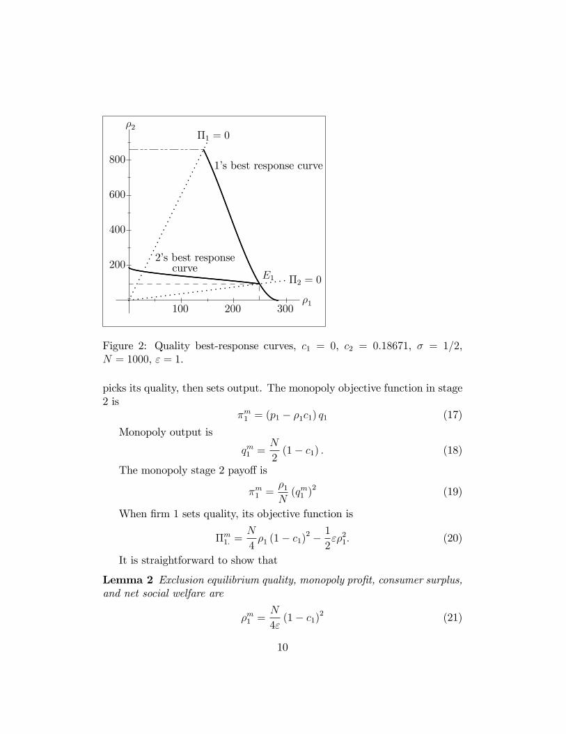
Figure 3 shows payoff functions for the parameter values of Figure 1, with theexception that σ = 1/4, so varieties are relatively poor horizontal substitutes.For ω = 0, the outcome is that of the basic model; the firms have identicalpayoffs. As ω rises, firm 2’s payoff falls. Firm 1’s payoff first rises, thenfalls, as a function of ω. Its payoff is maximized for a value of ω that allowsfirm 2 to operate with positive profit. Further, firm 1’s downstream duopolypayoff exceeds its exclusion payoff.Figure 4 shows the corresponding quality values. In downstream duopoly
equilibrium, ρ2 < ρ1 and ρ1 is less than firm 1’s exclusion quality. Despitethis, however, as shown in Figure 5, consumer surplus and net social welfareare both greater with both firms active in the downstream market than iffirm 1 excludes firm 2. Because variety 2 is a weak horizontal substitute forvariety 1, firm 1 finds it profitable to set ω so firm 1 stays in the market andpurchases a relatively large amount of the essential input. Because variety2 is a weak horizontal substitute for variety 1, firm 2’s sales do not much cutinto firm 1’s sales.
12

ω
ExclusionFirm 1
Firm 2
0.04 0.08 0.12 0.16 0.20 0.24 0.28 0.32 0.36 0.40 0.415
31250
33488
19111
0
...................................................................
.................................................
......................................................
..............................................................
..............................................................................
........................................................................................................................................
...............................................................................................................................................................................................................................................................................................................................................................
.................................................................................................................................................................................................................................................................................................................................................................................................................................................................................................................................................................................................................................................................................................................................................................................................................................
ω∗
Figure 3: Exclusion payoff, firm 1, and downstream duopoly payoffs, asfunctions of ω. ε = 1, σ = 1/4, N = 1000, c1 = c2 = 0. ω∗ indicates firm 1’sprofit-maximizing wholesale price.
13
ω
ρ
Exclusion
Firm 1
Firm 2
0.04 0.08 0.12 0.16 0.20 0.24 0.28 0.32 0.36 0.40 0.415
250
225.75237.42
0
...................................................................................................................................................................................................................................................................................................................................................................................................................................................................................................................................................................................................................................................................................................................................................................
...............................................................................................................................................................................................................................................................................................................................................................................................................................................................................................................................................................................................................................................................................................................................................................................................................
97.52
ω∗
Figure 4: Reservation prices, exclusion and downstream duopoly, as functionsof ω. ε = 1, σ = 1/4, N = 1000, c1 = c2 = 0. ω∗ indicates firm 1’s profit-maximizing wholesale price.
4.4 σ = 1/2
Now turn to the case that varieties are closer horizontal substitutes. Figure6 shows payoffs as functions of ω for the parameter values of Figure 1. Forω = 0, the outcome is that of the basic model; the firms have identicalpayoffs. As ω rises, Π1 increases and Π2 decreases, throughout the range forwhich Π2 ≥ 0; for higher values of ω, firm 2’s participation constraint wouldnot be met.But for the intermediate product differentiation level indicated by σ =
1/2, firm 1’s exclusion payoff exceeds its maximum duopoly payoff. Con-sumers’taste for variety is great enough for variety to maximize welfare, butthe two varieties are close enough substitutes that firm 1’s profit is greater ifit excludes firm 2 from the market.Figure 7 shows equilibrium quality levels for different wholesale prices,
for the parameter values of Figure 6. As we expect from Lemma 2, higherwholesale prices induce firm 1 to invest more in quality, and firm 2 less. Buteven for the value of ω for which firm 2’s participation constraint binds, firm1’s quality choice (242.31) is less than the quality it would choose (250) if itexcludes firm 2. If one measures market performance by quality, horizontal
14

ω
S, u
S: exclusion
u: exclusion
u
S
0.04 0.08 0.12 0.16 0.20 0.24 0.28 0.32 0.36 0.40 0.415
31250
62500
55741
93963
35517
71184
..........................................................................................................................................................................................................................................................................................................................................................................................................................................................................................................................................................................................................................................................................................................................................................................................
..................................................................................................................................................................................................................................................................................................................................................................................................................................................................................................................................................................................................................................................................................................................................................................................................
ω∗
Figure 5: Consumer surplus (S) and net social welfare (u), exclusion anddownstream duopoly, as functions of ω. ε = 1, σ = 1/4, N = 1000, c1 =c2 = 0. ω∗ indicates firm 1’s profit-maximizing wholesale price.
15

ω
Exclusion
Firm 1
Firm 2
0.02 0.04 0.06 0.08 0.10 0.12 0.14 0.16 0.18 0.20
31250
27270
11378
0
................................................................
.....................................................................
............................................................................
....................................................................................
................................................................................................
...................................................................................................................
.................................................................................................................................................
..............................................................................
....................................................................................................................................................................................................................................................................................................................................................................................................................................................................................................................................................................................................................................................................................................................................
Figure 6: Exclusion payoff, firm 1, and downstream duopoly payoffs, asfunctions of ω. ε = 1, σ = 1/2, N = 1000, c1 = c2 = 0.
exclusion is best.But neither economists nor antitrust authorities are wont to measure mar-
ket performance by quality alone. Rather, they focus on consumer surplus ornet social welfare, the sum of consumer surplus and firms’profits.11 Figure 8shows net social welfare (u) and consumer surplus (S) for the parameter val-ues of the second case. In this instance, there is no need to choose betweenconsumer surplus and net social welfare as measures of market performance;they yield the same result. Net social welfare and consumer surplus bothpeak for ω = 0 and fall steadily as ω rises. Further, net social welfare andconsumer surplus with two active firms are always greater than the corre-sponding exclusion values.The difference between the quality rankings of Figure 7 and the welfare
rankings of Figure 8 reflect the welfare gains from horizontal product dif-
11There is of course a debate whether consumer surplus or net social welfare is theappropriate index of market performance for policy purposes, but the terms of this debateare well known, and we do not enter into it here.
16

ω
ρ
ExclusionFirm 1
Firm 2
0.02 0.04 0.06 0.08 0.10 0.12 0.14 0.16 0.18 0.20
250
213.33
242.31
87.23
0
...........................................................................................................................................................................................................................................................................................................................................................................................................................................................................................................................................................................
.....................................................................................................................................
....................................................................................................................................................................................................................................................................................................................................................................................................................................................................................................................................................................................................................................................................................................................................
Figure 7: Reservation prices, exclusion and downstream duopoly, as functionsof ω. ε = 1, σ = 1/2, N = 1000, c1 = c2 = 0.
ferentiation if both varieties are present. For this set of parameter values,market performance is best, assuming production by firms, if both firms areactive and both firms have access to the essential input at its marginal costof production (which allows firm 1 to earn a normal rate of return on invest-ment).
5 Conclusion
In Trinko, the U.S. Supreme Court focused on quality competition – verticalproduct differentiation – as a driver of market performance. But, as thesaying goes, “variety is the spice of life,”and horizontal and vertical productdifferentiation both affect market performance. In the model explored here,if product varieties are weak horizontal substitutes, the vertically-integratedsupplier of an essential input will set the price of its intermediate good soits nonintegrated downstream competitor stays in the market. Because ofthe market power exercised by the vertically-integrated firm, the indepen-dent downstream firm will invest less in quality, but horizontal competitionincrease consumer surplus and net social welfare, compared with exclusion.If, on the other hand, varieties are close horizontal substitutes, the most prof-
17

ω
S, u
S: exclusion
u: exclusion
u
S
0.02 0.04 0.06 0.08 0.10 0.12 0.14 0.16 0.18 0.20
31250
62500
35914
63194
........................................................................................................................................................................................................................................................................................................................................................................................................................................................................................................................................................................................................................................................................................................................
...................................................................................................................................................................................................................................................................................................................................................................................................................................................................................................................................................................................................................................................................................................................
Figure 8: Consumer surplus (S) and net social welfare (u), exclusion anddownstream duopoly, as functions of ω. ε = 1, σ = 1/2, N = 1000, c1 =c2 = 0.
itable path for the vertically-integrated supplier is to refuse to deal with thenonintegrated downstream firm. The vertically-integrated firm’s monopolyquality is greater than its duopoly quality, if it were to price the intermediategood so the downstream rival just breaks even. But the loss of horizontalvariety entailed by exclusion again reduces consumer surplus and net socialwelfare.What is meant by the term “competition” in discussions of antitrust
policy is often unclear, encompassing competitive market structure, potentialcompetition, actual rivalry in the product market, and competitive marketperformance. The upshot of the analysis presented here is that it is actualrivalry in the development of high-quality substitute varieties that promotesconsumer welfare, and that such rivalry is ill-served by the exercise of marketpower in input markets and by the refusal of vertically-integrated upstreamfirms with their nonintegrated downstream rivals.
18

6 Appendix
6.1 Horizontal competition
6.1.1 Stage 2
Substituting the inverse demand equation (1) into the objective function (6),firm 1’s product-market objective function is
π1 = ρ1
[1− c1 −
1
N
(q1 + σ
√ρ2
ρ1
q2
)]q1 (31)
The first-order condition to maximize π1 is
1− c1 −1
N
(2q1 + σ
√ρ2
ρ1
q2
)= 0, (32)
from which we get (7).The first-order condition can be rewritten as
2q1 + σ
√ρ2
ρ1
q2 = N (1− c1) . (33)
In the same way, firm 2’s stage 2 first-order condition can be written
σ
√ρ1
ρ2
q1 + 2q2 = N (1− c2) . (34)
Solving the two first-order conditions, equilibrium outputs are
q̂1 = N2 (1− c1)− σ
√ρ2ρ1
(1− c2)
4− σ2(35)
q̂2 = N2 (1− c2)− σ
√ρ1ρ2
(1− c1)
4− σ2. (36)
(35) and (36) are substituted in (8) to obtain expressions for stage 1objective functions.From (35) and (36), the conditions for both outputs to be nonnegative
are2
σ≥ 1− c2
1− c1
√ρ2
ρ1
≥ σ
2, (37)
where the first inequality is the condition for q1 to be nonnegative and thesecond inequality is the condition for q2 to be nonnegative.
19

6.1.2 Stage 1
6.1.3 Comparative statics
We are interested in comparative statics with respect to c2. Differentiatingthe quality first-order conditions ∂Π1
∂ρ1≡ 0 and ∂Π2
∂ρ2≡ 0 with respect to c2
gives the system of equations ∂2Πdd1
∂ρ21
∂2Πdd1
∂ρ1∂ρ2∂2Πdd
2
∂ρ1∂ρ2
∂2Πdd2
∂ρ22
( ∂ρ1∂c2∂ρ2∂c2
)= −
(∂2Πdd
1
∂c2∂ρ1∂2Πdd
2
∂c2∂ρ2
). (38)
Assuming stability gives that the trace of the coeffi cient matrix on theleft is negative, and its determinant positive. Suffi cient conditions for thetrace to be negative are that the diagonal elements of the coeffi cient matrixbe negative, which we would have in any event from the assumption that thesecond-order condition is met.Tedious evaluation of the derivatives in (38) establishes the following sign
pattern if the equation is multiplied by the inverse of the coeffi cient matrixon the right: (
∂ρ1∂c2∂ρ2∂c2
)=
(− ++ −
)(−+
), (39)
Then the signs of the derivatives satisfy
∂ρ1
∂c2
= (−) (−) + (+) (+) > 0 (40)
and∂ρ2
∂c2
= (+) (−) + (−) (+) < 0, (41)
and this establishes the first part of Lemma 1. As c2 rises, equilibrium ρ1
rises and ρ2 falls.For the slope of the firm 1’s best-response equation, the first-order con-
dition can be written
∂Πdd1 (ρ1, ρ2)
∂ρ1
= 2N2 (1− c1)− σ
√ρ2ρ1
(1− c2)
4− σ2
1− c1
4− σ2− ερ1 = 0. (42)
20

Then∂2Πdd
1
∂ρ21
= Nσ (1− c1) (1− c2)
(4− σ2)2 ρ−3/21 ρ
1/22 − ε < 0, (43)
where the sign follows from the second-order condition, and
∂2Πdd1
∂ρ1∂ρ2
= −N σ (1− c1) (1− c2)
(4− σ2)2 ρ−1/21 ρ
−1/22 < 0 (44)
Differentiate the first-order condition to obtain the slope of the best-response function:
∂2Πdd1
∂ρ21
dρ1
dρ2
∣∣∣∣brf
+∂2Πdd
1
∂ρ1∂ρ2
= 0
dρ1
dρ2
∣∣∣∣brf
=
∂2Πdd1
∂ρ1∂ρ2
−∂2Πdd1
∂ρ21
< 0. (45)
This is the second part of Lemma 1.
6.2 Vertical competition
6.2.1 Quality
For the case that firm 1 is vertically integrated, stage 2 equilibrium outputsare
q̂1 = N2 (1− c1)− σ
√ρ2ρ1
(1− c2 − ω)
4− σ2(46)
and
q̂2 = N2 (1− c2 − ω)− σ
√ρ1ρ2
(1− c1)
4− σ2. (47)
These may be compared with (35) and (36). Substitution of these expressionsfor equilibrium outputs into (27) and into (8) (for i = 2) give the stage 1objective functions of firm 1 and firm 2, respectively.Theorem 4:
dΠdd2
dω=∂Πdd
2
∂ρ1
dρ1
dω+∂Πdd
2
∂ρ2
dρ2
dω+∂Πdd
2
∂ω
=∂Πdd
2
∂ρ1
dρ1
dω+∂Πdd
2
∂ω, (48)
21

since ∂Πdd2
∂ρ2= 0 (an application of the envelope theorem). From Lemma 3,
dρ1dω
> 0.Firm 2’s quality objective function is
Πdd2 =
1
Nρ̂2q
22 −
1
2ερ2
2, (49)
where output is given by (47). Then
∂Πdd2
∂ρ1
=2
Nρ2q2
∂q2
∂ρ1
< 0,
∂Πdd2
∂ω=
2
Nρ2q2
∂q2
∂ω< 0,
and for dΠdd2
dωwe have
signdΠdd
2
dω= (−) (+) + (−) < 0.
This is the first part of Theorem 4.For the second part of Theorem 4, again using the envelope theorem and
Lemma 3,dΠdd
1
dω=∂Πdd
1
∂ρ2
dρ2
dω+∂Πdd
1
∂ω=∂Πdd
1
∂ρ2
(−) +∂Πdd
1
∂ω.
From (27),∂Πdd
1
∂ρ2
=
2
Nρ1q1N
−12σρ
−1/21 ρ
−1/22 (1− c2 − ω)
4− σ2+ ω
(q2 + ρ2N
12σρ
1/21 ρ
−3/22 (1− c1)
4− σ2
)(and collecting terms in ω on the right)
= −q1σρ
1/21 ρ
−1/22 (1− c2)
4− σ2+ ω
{q2 +
[q1 +
1
2N
(1− c1)
4− σ2
]σρ
1/21 ρ
−1/22
4− σ2
}.
The coeffi cient of ω is positive. Hence
∂Πdd1
∂ρ2
< 0
22

for ω = 0, and ∂Πdd1
∂ρ2falls in magnitude as ω rises. This gives us
signdΠdd
1
dω=∂Πdd
1
∂ρ2
(−) +∂Πdd
1
∂ω= (−) (−) +
∂Πdd1
∂ω,
for ω near 0, so that the first term on the right is positive for ω = 0, eventuallyturning negative.Taking the derivative of (27) with respect to ω gives,
1
N
∂Πdd1
∂ω=
2σρ1/21 ρ
1/22 N
2 (1− c1)− σ (1− c2) ρ−1/21 ρ
1/22
(4− σ2)2 +ρ2N2 (1− c2)− σρ1/2
1 ρ−1/22 (1− c1)
4− σ2
− 2ωρ2
4− σ2
8− 3σ2
4− σ2.
The fractions on the right in the first two terms of the expression for ∂Πdd1
∂ω
are q1 (0) and q2 (0), respectively. If q2 > 0 for ω > 0, it is positive for ω = 0.If we assume as well q1 (0) ≥ 0, then
signdΠdd
1
dω= (−) (−) + (+)
for ω near 0, with the first term on the right positive for ω = 0, eventuallyturning negative. The slope of the profit function may be positive throughoutthe range of ω where firm 2’s participation constraint is satisfied, or it mayturn negative within this region. This is the second part of Theorem 4.
References
[1] Aghion, Phillippe, Bloom, Nick, Blundell, Richard, Griffi th, Rachel andHowitt, Peter (2005). “Competition and innovation: an inverted-U re-lationship.”Quarterly Journal of Economics 120:701—728.
[2] Anderson, Simon P., de Palma, André and Thisse, Jacques—François(1992). Discrete Choice Theory of Product Differentiation. Cambridge,Massachusetts: MIT Press.
23

[3] Hicks, J. R. (1935). “Annual survey of economic theory: the theory ofmonopoly.”Econometrica 3:1-20.
[4] Motta, Massimo (1993). “Endogenous quality choice: price vs. quantitycompetition.”Journal of Industrial Economics 41:113-131.
[5] Mussa, Michael and Rosen, Sherwin “Monopoly and product quality”(1978). Journal of Economic Theory 18:301—317.
[6] Neven, Damien (1986). “‘Address’models of differentiation,” in Nor-man, George, editor Spatial Pricing and Differentiated Markets. Lon-don: Pion Limited, 5—18.
[7] Schumpeter, Joseph A.(1934). The Theory of Economic Development.Cambridge, Massachusetts: Harvard University Press..
[8] – Capitalism, Socialism and Democracy. (1943). London: Allen & Un-win, 1943.
[9] Spence, A. Michael (1976). “Product differentiation and welfare,”Amer-ican Economic Review 66:407—414.
[10] Sutton, John (1991). Sunk costs and Market Structure. Cambridge,Massachusetts: MIT Press.
[11] – Technology and Market Structure. Cambridge, Massachusetts: MITPress, 1998.
[12] Villard, Henry H.(1958). “Competition, oligopoly, and research.”Jour-nal of Political Economy 66:483—497.
[13] Waterson, Michael (1989). “Models of product differentiation.”Bulletinof Economic Research 41: 1-27.
[14] Wauthy, Xavier (1996). “Quality choice in models of vertical differenti-ation.”Journal of Industrial Economics 44:345—353.
[15] Winter, Sidney G. (1984). “Schumpeterian competition in alternativetechnological regimes.”Journal of Economic Behavior and Organization5:287—320.
24