Embed Size (px)
Citation preview
Kosrae Utilities Authority
Cost of Service and Tariff Study
FinalReport
submitted to: Kosrae Utilities Authority (KUA)
submitted by: KEMA Inc.
1October 2012

Kosrae Utilities Authority Proprietary Cost of Service Study – Final Report 1 October 2012
2
FREEDOM OF INFORMATION ACT (FOIA) NOTICE: This document contains trade secrets
and/or proprietary, commercial, or financial information not generally available to the public. It is
considered privileged and proprietary to the Offeror, and is submitted by KEMA, Inc./KEMA-
XENERGY in confidence with the understanding that its contents are specifically exempted from
disclosure under the Freedom of Information Act [5 USC Section 552 (b) (4)] and shall not be
disclosed by the recipient [whether it be Government (local, state, federal, or foreign), private
industry, or non-profit organization] and shall not be duplicated, used, or disclosed, in whole or
in part, for any purpose except to the extent in which portions of the information contained in this
document are required to permit evaluation of this document, without the expressed written
consent of the Offeror. If a contract is awarded to this Offeror as a result of, or in connection
with, the submission of this data, the right to duplicate, use, or disclose the data is granted to
the extent provided in the contract.

Kosrae Utilities Authority Proprietary Cost of Service Study – Final Report 1 October 2012
3
Table of Contents
1 Introduction ......................................................................................................... 4
1.1 Project Background............................................................................................................ 4
1.2 Approach for this Study ...................................................................................................... 4
1.3 Report Outline ................................................................................................................... 5
2 KUA Financial Model ........................................................................................... 6
2.1 General overview of the model............................................................................................ 6
2.2 Model Assumptions............................................................................................................ 8
2.3 Financial Targets ............................................................................................................. 19
3 Analysis of KUA Tariff Levels ........................................................................... 22
3.1 Scenario 1: Existing Tariffs ............................................................................................... 22
3.2 Scenario 2: Tariff Increase for 10% ROC ........................................................................... 25
3.3 Scenario 3: Grant-funded Investment ................................................................................ 27
3.4 Summary of Scenario Results........................................................................................... 30
4 Analysis of KUA Tariff Structure ...................................................................... 32
4.1 Cost Allocation Analysis ................................................................................................... 32
4.2 Analysis of Existing KUA Tariffs ........................................................................................ 41
4.3 Development of Alternative Tariff Structure ........................................................................ 43
5 Conclusions and Recommendations................................................................ 50
5.1 Conclusions..................................................................................................................... 50
5.2 Recommendations ........................................................................................................... 51
Annex 1: Demand data used for deriving load profiles .......................................... 53
Annex 2: Cost of Capital ......................................................................................... 55
Kosrae Utilities Authority Proprietary Cost of Service Study – Final Report 1 October 2012
4
1 Introduction
1.1 Project Background
Kosrae Utilities Authority (KUA) is a vertically integrated utility that supplies electrical power to
the State of Kosrae, Micronesia. In the year 2011, KUA served 1,870 customers with a demand
of 5,248,361 kWh. The peak load in that year was 1.06 MW.
The company is heavily dependent on external financing (grants) for undertaking investments.
Most of the company’s assets have been funded by grants from the USA and other states.
KUA’s base tariff has not been reviewed and/or adjusted since 1991 and it is opportune to
review the tariff in the fore field of possible private sector participation in the electricity industry
in the Kosrae State. The review based on the findings will be required to provide
recommendations on an appropriate tariff structure and on mechanisms to adjust the tariffs.
In this context KUA has asked DNV KEMA through the Pacific Power Associated (PPA) to
undertake a study to review the current base tariff applied by KUA and recommend a tariff
structure that balances the interest of consumers and the utility.
This Final Report presents the results of the analysis conducted by DNV KEMA and presents
the possible options that KUA could consider to change the existing tariffs. The Draft version of
this report has been presented and discussed with KUA and other stakeholders in the week of
25 September 2012. Based on this the draft version was further refined resulting in this Final
Report.
1.2 Approach for this Study
During the Inception Phase of this project an assessment was made of the existing tariff policies
and procedures as well as of the available data and information. Based on this the following
approach was proposed and subsequently carried out after approval by the client:
Kosrae Utilities Authority Proprietary Cost of Service Study – Final Report 1 October 2012
5
1. Tariff Level Analysis: KUA’s financial performance has been modeled and evaluated to
evaluate the effectiveness of the existing tariff level. For this purpose KEMA has
developed a financial model in the form of a spreadsheet model, which has incorporated
capital and operational expenditures and income sources in order to identify financial
performance and robustness of the company. Using the model different options to
increase tariffs to assure sustainable financial performance of KUA have been
evaluated.
2. Tariff Structure Analysis: An analysis has been performed to evaluate the existing
tariff structure in use by KUA. This has provided insight into the extent to which the
existing tariffs can be considered in line with the true costs associated with each
customer group i.e. to what extent the tariffs for each customer reflect the true costs of
providing supply. From an economic point of view an alignment between costs and tariff
is desired as cost reflectiveness helps to promote efficiency. Based on this an alternative
tariff structure for KUA has been developed.
1.3 Report Outline
The remaining of this report is structured as follows:
• Section 2 presents an overview on the financial model that has been developed and sets
out the underlying modeling assumptions and data. In this chapter also the indicators
and targets for evaluating financial performance are presented.
• Section 3 presents the results of the financial analysis that were performed making use
of the model developed in Section 2. The gap in financial performance between current
and desired tariff levels is assessed and possible tariff increase scenarios discussed.
• Section 4 deals with the tariff structure. A cost allocation analysis is performed to
investigate the extent to which the current tariff structure is in line with the actual costs
allocated to each customer category. Also here alternative tariff structures are
investigated.
• Section 5 closes with the conclusions and presents the recommendations of this study.
Kosrae Utilities Authority Proprietary Cost of Service Study – Final Report 1 October 2012
6
2 KUA Rate Setting Model
2.1 General overview of the model
The KUA Rate Setting Model simulates revenues and costs and based on this, derives
forecasts for Profit and Loss (P&L), Balance Sheet (BS), and Cash Flow (CF) statements as
well as for key financial indicators. The format of these statements is kept the same as the
published financial accounts by KUA.
Financial data for the financial years 2009/10 and 2010/11 have been used as the model’s
starting point. These are inserted as hard data into the model. From there on the financial model
simulates the financial statements and indicators for the next 10 years i.e. until financial year
2021/22. This simulation can be performed under the assumption of different scenarios and
parameter settings.
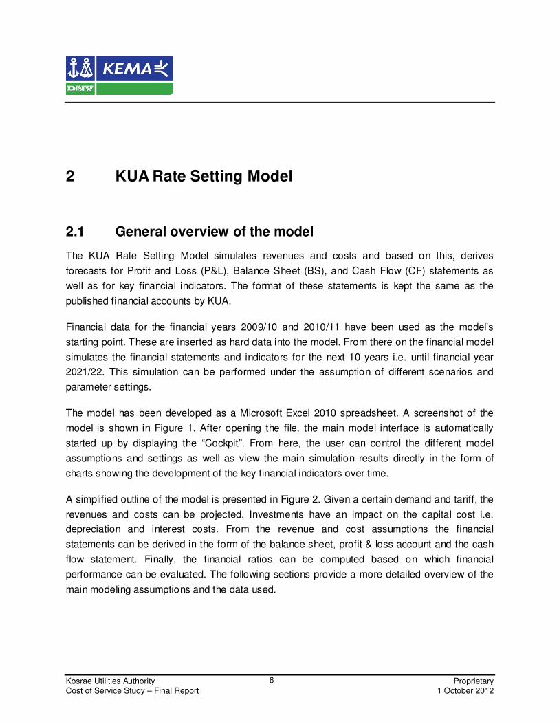
The model has been developed as a Microsoft Excel 2010 spreadsheet. A screenshot of the
model is shown in Figure 1. After opening the file, the main model interface is automatically
started up by displaying the “Cockpit”. From here, the user can control the different model
assumptions and settings as well as view the main simulation results directly in the form of
charts showing the development of the key financial indicators over time.
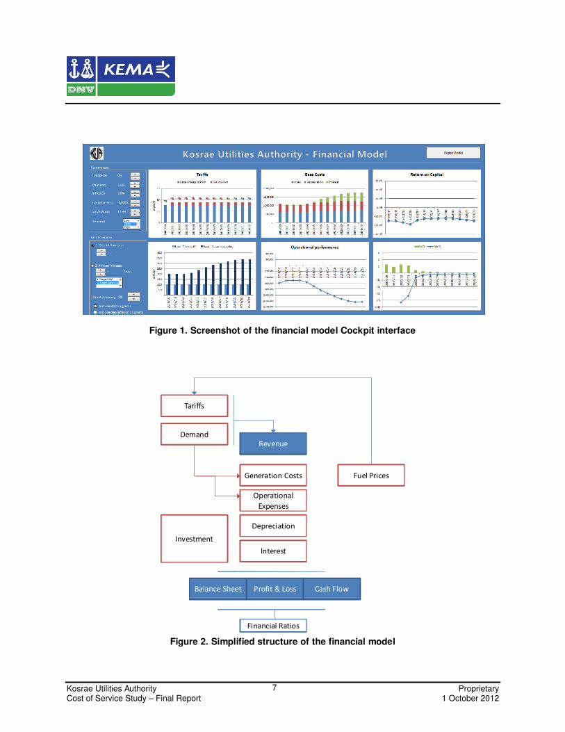
A simplified outline of the model is presented in Figure 2. Given a certain demand and tariff, the
revenues and costs can be projected. Investments have an impact on the capital cost i.e.
depreciation and interest costs. From the revenue and cost assumptions the financial
statements can be derived in the form of the balance sheet, profit & loss account and the cash
flow statement. Finally, the financial ratios can be computed based on which financial
performance can be evaluated. The following sections provide a more detailed overview of the
main modeling assumptions and the data used.
Kosrae Utilities Authority Proprietary Cost of Service Study – Final Report 1 October 2012
7
Figure 1. Screenshot of the financial model Cockpit interface
Figure 2. Simplified structure of the financial model
Demand
Generation Costs
Tariffs
Operational
Expenses
Balance Sheet
Depreciation
Interest
Profit & Loss Cash Flow
Revenue
Fuel Prices
Investment
Financial Ratios
Kosrae Utilities Authority Proprietary Cost of Service Study – Final Report 1 October 2012
8
2.2 Model Assumptions
2.2.1 Demand
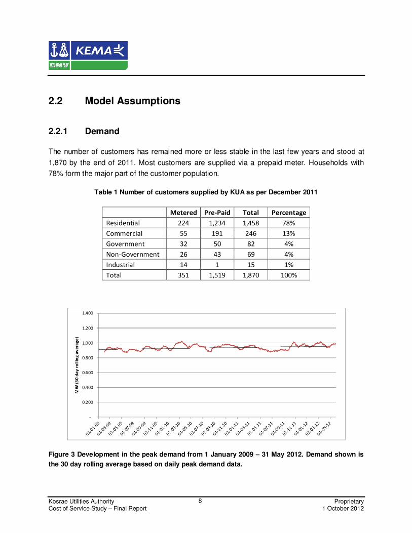
The number of customers has remained more or less stable in the last few years and stood at
1,870 by the end of 2011. Most customers are supplied via a prepaid meter. Households with
78% form the major part of the customer population.
Table 1 Number of customers supplied by KUA as per December 2011
Metered Pre-Paid Total Percentage
Residential 224 1,234 1,458 78%
Commercial 55 191 246 13%
Government 32 50 82 4%
Non-Government 26 43 69 4%
Industrial 14 1 15 1%
Total 351 1,519 1,870 100%
Figure 3 Development in the peak demand from 1 January 2009 – 31 May 2012. Demand shown is
the 30 day rolling average based on daily peak demand data.
-
0.200
0.400
0.600
0.800
1.000
1.200
1.400
MW
(3
0 d
ay
roll
ing
av
era
ge
)
Kosrae Utilities Authority Proprietary Cost of Service Study – Final Report 1 October 2012
9
The system peak load in 2011 was 1.22 MW and the average load factor is around 60%. Peak
demand has remained more or less flat in recent years as shown inFigure 3. For the future
some new projects on the island are envisaged which will tend to increase demand such as a
new hospital. For the immediate coming three years demand however demand will remain flat.
Demand forecast is set at zero-growth under the base case. During the analysis demand
variation will nevertheless be included by considering annual increase/decrease levels. For the
purpose of analysis a High and Low demand growth scenario have been assumed as well.
These correspond to respectively +2% and -2% demand growth.
2.2.2 Tariffs
KUA’s existing tariffs consist of two components:
• The Base Tariff, which is adjusted on an annual basis and is intended to cover the base
costs of the company including a part of the fuel costs;
• The Fuel Adjustment Charge (FAC), which is adjusted monthly and is intended to cover
the fuel costs in excess of the portion covered in the tariff rate.
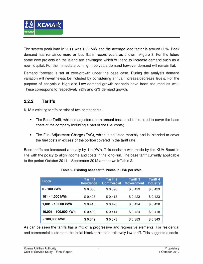
Base tariffs are increased annually by 1 ct/kWh. This decision was made by the KUA Board in
line with the policy to align income and costs in the long-run. The base tariff currently applicable
to the period October 2011 – September 2012 are shown inTable 2.
Table 2. Existing base tariff. Prices in USD per kWh.
Block Tariff 1
Residential Tariff 2
Commercial Tariff 3
Government Tariff 4
Industry
0 - 100 kWh $ 0.358 $ 0.398 $ 0.423 $ 0.423
101 - 1,000 kWh $ 0.403 $ 0.413 $ 0.423 $ 0.423
1,001 - 10,000 kWh $ 0.416 $ 0.423 $ 0.434 $ 0.428
10,001 - 100,000 kWh $ 0.409 $ 0.414 $ 0.424 $ 0.418
> 100,000 kWh $ 0.349 $ 0.373 $ 0.383 $ 0.343
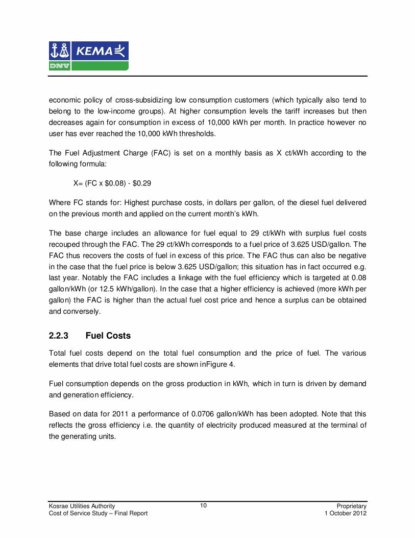
As can be seen the tariffs has a mix of a progressive and regressive elements. For residential
and commercial customers the initial block contains a relatively low tariff. This suggests a socio-
Kosrae Utilities Authority Proprietary Cost of Service Study – Final Report 1 October 2012
10
economic policy of cross-subsidizing low consumption customers (which typically also tend to
belong to the low-income groups). At higher consumption levels the tariff increases but then
decreases again for consumption in excess of 10,000 kWh per month. In practice however no
user has ever reached the 10,000 kWh thresholds.
The Fuel Adjustment Charge (FAC) is set on a monthly basis as X ct/kWh according to the
following formula:
X= (FC x $0.08) - $0.29
Where FC stands for: Highest purchase costs, in dollars per gallon, of the diesel fuel delivered
on the previous month and applied on the current month’s kWh.
The base charge includes an allowance for fuel equal to 29 ct/kWh with surplus fuel costs
recouped through the FAC. The 29 ct/kWh corresponds to a fuel price of 3.625 USD/gallon. The
FAC thus recovers the costs of fuel in excess of this price. The FAC thus can also be negative
in the case that the fuel price is below 3.625 USD/gallon; this situation has in fact occurred e.g.
last year. Notably the FAC includes a linkage with the fuel efficiency which is targeted at 0.08
gallon/kWh (or 12.5 kWh/gallon). In the case that a higher efficiency is achieved (more kWh per
gallon) the FAC is higher than the actual fuel cost price and hence a surplus can be obtained
and conversely.
2.2.3 Fuel Costs
Total fuel costs depend on the total fuel consumption and the price of fuel. The various
elements that drive total fuel costs are shown inFigure 4.
Fuel consumption depends on the gross production in kWh, which in turn is driven by demand
and generation efficiency.
Based on data for 2011 a performance of 0.0706 gallon/kWh has been adopted. Note that this
reflects the gross efficiency i.e. the quantity of electricity produced measured at the terminal of
the generating units.

Kosrae Utilities Authority Proprietary Cost of Service Study – Final Report 1 October 2012
11
Figure 4 Factors determining fuel costs
Demand follows automatically from the selected demand scenario. All parameters are modeled
as variables and can be adjusted in the model to investigate the impact of changes in the
production mix and fuel price on prices.
Losses consist of two parts namely station losses and distribution losses. Station losses relate
to the energy consumed by the power plant itself in producing the net energy output delivered to
the grid. Distribution losses consist of technical and non-technical losses. Technical losses are
the losses occurring in the various network assets due to thermal and magnetic phenomena
while non-technical losses relate to metering and billing errors. The base assumptions regarding
station and network losses together are 17.9% based on data for 2011. In the model it is
possible to project a reduced level of losses over time.
Fuel costs
Fuel consumption
(gallons)
Gross production
(kWh)
Demand (kWh) Losses (kWh)
Station losses (kWh)
Distribution losses (kWh)
Generation efficiency
(gallon/kWh)
Fuel price (USD/gallon)

Kosrae Utilities Authority Proprietary Cost of Service Study – Final Report 1 October 2012
12
Fuel prices for 2011 are taken as the average price incurred by KUA during the financial year
2011 (USD 4.34/gallon1). For each subsequent year prices are projected by selecting an oil
price scenario. Note further thatall fuel-related costs are included in this price (i.e. lubricants and
fuel conditioning). In the case of KUA these form about 2% of the total fuel costs. In the model
fuel prices are by default assumed to be fixed but can be increased or decreased as required.
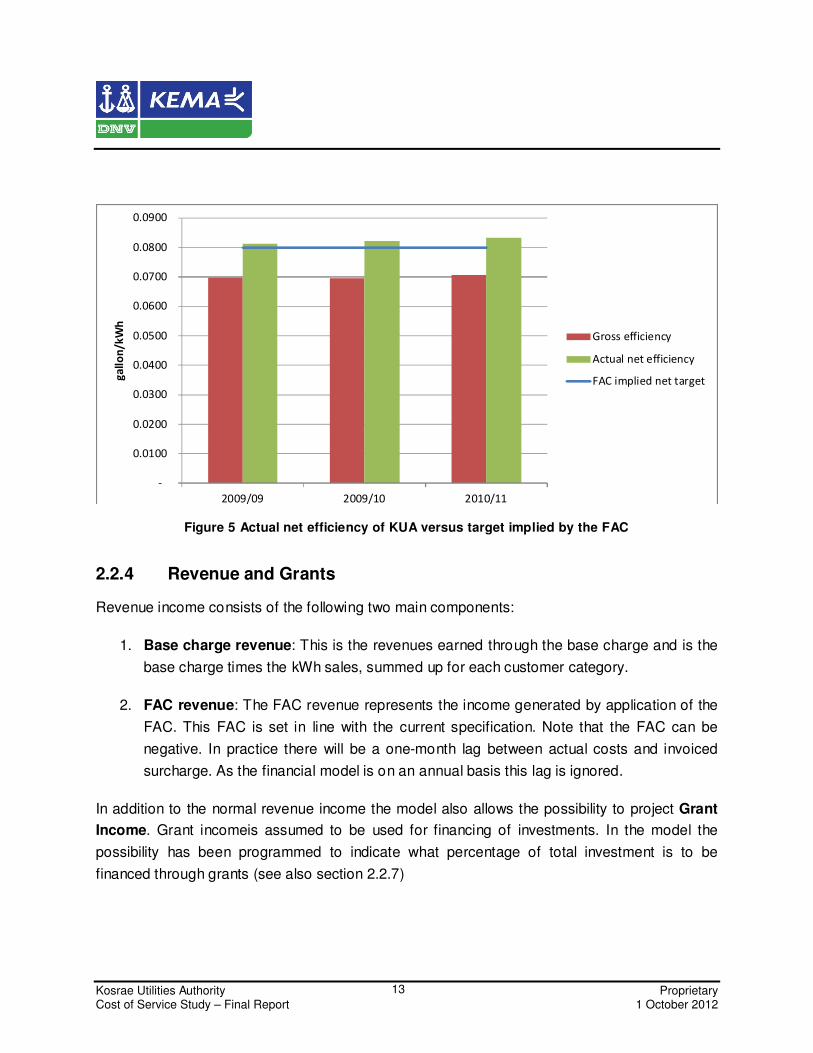
Note that the 0.08 gallon/kWh in the FAC formula considers the net efficiency i.e. the number of
gallons used to deliver 1 kWh to the final customer. This number thus includes the gross
efficiency (conversion of fuel into electricity at the power plant) and the losses (station and
distribution losses). As mentioned earlier the gross efficiency in KUA in 2011 was 0.0706
gallon/kWh. The actual net efficiency was 0.0832 gallon/kWh which is less than the target of
0.08 implied in the FAC formula. This suggests that KUA is making a loss on the FAC front.
Table 3. Fuel consumption versus gross production and sales. Gross efficiency is defined as fuel
consumption divided by gross production. Net efficiency is fuel consumption divided by sales.
.
1 Total fuel consumption was 436,894 gallons at a cost of USD 1,894,071. Note that these totals also include the
gallon consumption and cost for fuel used for vehicles as well as costs for lubricants and others.
2009/09 2009/10 2010/11
Fuel gallon 420,372 452,628 436,894
Gross Production kWh 6,022,171 6,504,201 6,188,752
Losses kWh 852,813 991,475 940,391
Sales kWh 5,169,358 5,512,726 5,248,361
Gross efficiency gallon/kWh 0.0698 0.0696 0.0706
Net efficiency gallon/kWh 0.0813 0.0821 0.0832
Kosrae Utilities Authority Proprietary Cost of Service Study – Final Report 1 October 2012
13
Figure 5 Actual net efficiency of KUA versus target implied by the FAC
2.2.4 Revenue and Grants
Revenue income consists of the following two main components:
1. Base charge revenue: This is the revenues earned through the base charge and is the
base charge times the kWh sales, summed up for each customer category.
2. FAC revenue: The FAC revenue represents the income generated by application of the
FAC. This FAC is set in line with the current specification. Note that the FAC can be
negative. In practice there will be a one-month lag between actual costs and invoiced
surcharge. As the financial model is on an annual basis this lag is ignored.
In addition to the normal revenue income the model also allows the possibility to project Grant
Income. Grant incomeis assumed to be used for financing of investments. In the model the
possibility has been programmed to indicate what percentage of total investment is to be
financed through grants (see also section 2.2.7)
-
0.0100
0.0200
0.0300
0.0400
0.0500
0.0600
0.0700
0.0800
0.0900
2009/09 2009/10 2010/11
ga
llo
n/k
Wh
Gross efficiency
Actual net efficiency
FAC implied net target

Kosrae Utilities Authority Proprietary Cost of Service Study – Final Report 1 October 2012
14
2.2.5 Operating Expenses
The starting point for operating expenses (excluding fuel and depreciation which are treated
separately) is the historical opex record as observed from the financial accounts. In order to
derive the forecast for opex, demand has been adopted as the main opex driver.
In developing opex forecasts one also needs to take into account the fact that opex levels are
affected by general inflation trends. Over time, the nominal prices of goods and services
procured by KUA will increase and this will have an upward effect on its opex. For inflation a
value of 3% has been adopted based on the latest available information for the year 2010.2
Operational Efficiency
Productivity improvement is modeled by an annual decrease in the required costs per kWh. The
increase in efficiency can come through two fundamental routes. First, productivity can be
increased up to the level of so-called best-practice performance. Initially, it is fair to assume that
KUA is not as efficient as the most efficient similar sized electric island utilities in the world.
These most efficient utilities would determine the so-called productivity frontier. The distance
between KUA’s actual productivity performance and the frontier is a measure of the efficiency
improvement potential that could be achieved. Second, over time, due to ongoing technological
improvements, the productivity frontier itself will also shift. That is, even the most efficient
utilities will become more efficient over time. This is also referred to as dynamic efficiency
improvement.
In order to establish the expected increase opex efficiency, one should take into account that
improvement is a continuous process over time rather than a one-off event. For the base case,
the assumption is that KUA has potential to improve its efficiency at a level of 1% per annum.
2 Source: World Bank, http://www.tradingeconomics.com/micronesia/inflation-gdp-deflator-annual-percent-wb-
data.html
Kosrae Utilities Authority Proprietary Cost of Service Study – Final Report 1 October 2012
15
The opex forecast is dependent on the choice of demand forecast with costs increasing more
under the high scenario and vice versa.
2.2.6 Investment and Depreciation
Based on projected capex, depreciation costs and net asset values (book values) for new
investments have been computed. The assumption is made that no disposals (capital exits) take
place. Investments forecasts have been obtained from KUA’s forecasts. A distinction is made
between (1) existing investment and (2) new investment.
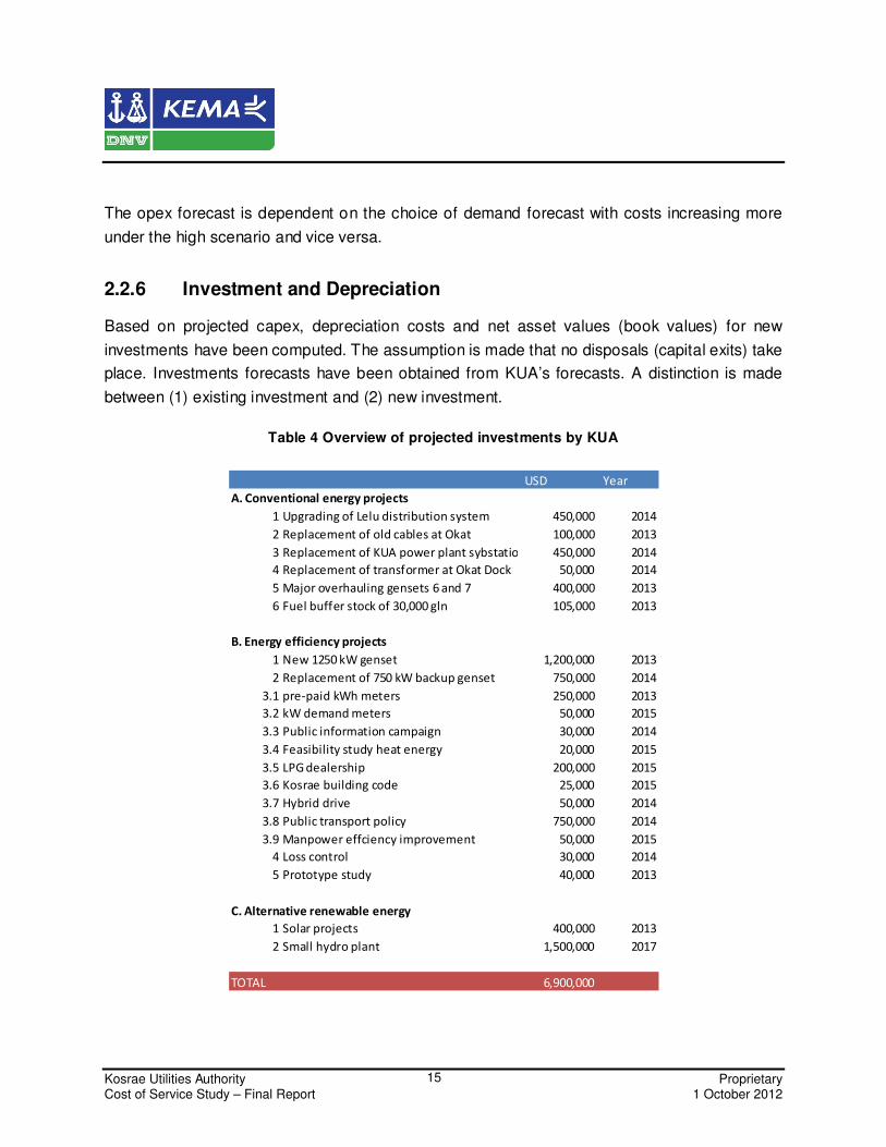
Table 4 Overview of projected investments by KUA
USD Year
A. Conventional energy projects
1 Upgrading of Lelu distribution system 450,000 2014
2 Replacement of old cables at Okat 100,000 2013
3 Replacement of KUA power plant sybstation 450,000 2014
4 Replacement of transformer at Okat Dock 50,000 2014
5 Major overhauling gensets 6 and 7 400,000 2013
6 Fuel buffer stock of 30,000 gln 105,000 2013
B. Energy efficiency projects
1 New 1250 kW genset 1,200,000 2013
2 Replacement of 750 kW backup genset 750,000 2014
3.1 pre-paid kWh meters 250,000 2013
3.2 kW demand meters 50,000 2015
3.3 Public information campaign 30,000 2014
3.4 Feasibility study heat energy 20,000 2015
3.5 LPG dealership 200,000 2015
3.6 Kosrae building code 25,000 2015
3.7 Hybrid drive 50,000 2014
3.8 Public transport policy 750,000 2014
3.9 Manpower effciency improvement 50,000 2015
4 Loss control 30,000 2014
5 Prototype study 40,000 2013
C. Alternative renewable energy
1 Solar projects 400,000 2013
2 Small hydro plant 1,500,000 2017
TOTAL 6,900,000
Kosrae Utilities Authority Proprietary Cost of Service Study – Final Report 1 October 2012
16
Existing investments are reflected in the balance sheet as per 30 September 2011. The
depreciation in 2010/11 is used as the starting point. Depreciation costs for existing investments
are projected to slightly decrease over time, reflecting the fact that some assets have been fully
depreciated and therefore removed from the net asset base.
New investments are those undertaken after 30 September 2011. New depreciation is derived
from the level of projected investments and is computed on the basis of straight-line
depreciation. An average depreciation period of 25 years is assumed based on the analysis of
depreciation periods and remaining asset lives in KUA’s existing asset base.
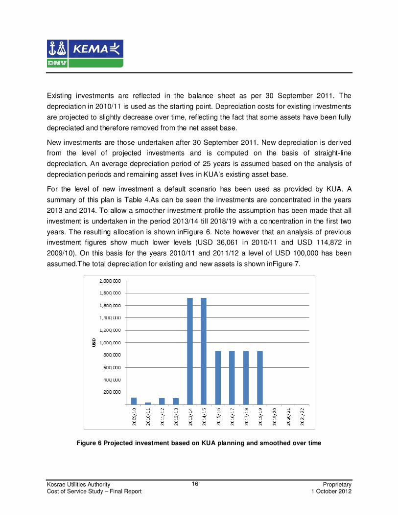
For the level of new investment a default scenario has been used as provided by KUA. A
summary of this plan is Table 4.As can be seen the investments are concentrated in the years
2013 and 2014. To allow a smoother investment profile the assumption has been made that all
investment is undertaken in the period 2013/14 till 2018/19 with a concentration in the first two
years. The resulting allocation is shown inFigure 6. Note however that an analysis of previous
investment figures show much lower levels (USD 36,061 in 2010/11 and USD 114,872 in
2009/10). On this basis for the years 2010/11 and 2011/12 a level of USD 100,000 has been
assumed.The total depreciation for existing and new assets is shown inFigure 7.
Figure 6 Projected investment based on KUA planning and smoothed over time

Kosrae Utilities Authority Proprietary Cost of Service Study – Final Report 1 October 2012
17
Figure 7 Projected depreciation for existing and new assets
2.2.7 Investment Funding
Financing of new investment is modeled in terms of two options, to be selected by the user.
Option 1: Own funding
Under this option financing of new investment is assumed to take place by KUA itself through a
mix of equity and long-term debt. A base case of 66% / 33% debt/equity allocation is assumed.
This allocation can be changed in the model. For the debt part (66%) an interest rate of 7.5%
and a repayment period of 10 years has been assumed. The remainder of the financing
requirement is assumed to come from equity (through cash reserves or alternatively short-term
loans).
Option 2: Grant funding
The second option is to have all investment financed through external grant funds. Under this
option the grant is treated as income under the profit & loss account and hence results in an

Kosrae Utilities Authority Proprietary Cost of Service Study – Final Report 1 October 2012
18
increase in net assets. The asset obtained through the grant is booked under the assets side of
the balance and depreciated annually.
2.2.8 Working Capital
With respect to working capital assumptions are made for the following balance sheet elements:
• Inventories change in proportion to the net asset value
• Receivables and payables change in proportion to tariff revenue
Current loans are used for the financing of working capital. In the modeling the assumption is
that changes in current loans are set equal to changes in working capital. Effectively the net
effect on the cash flow is thus zero.
2.2.9 Other assumptions
In addition to above some additional assumptions have been made:
• Cash: The assumption is that KUA targets to maintain a cash balance of USD 150,000.
This value can be changed in the model.
• Taxes: Corporate profits are not subject to income tax in the Federated States of
Micronesia. There is a gross receipt tax of 3% on revenues. KUA is however specifically
exempt from this tax or any other taxes such as taxes on property, operations, or
activities imposed by the Government.
• Exchangerate: All figures are nominated in United States Dollars.
2.2.10 Summary of Main Model Parameters
A summary of the default values for the main model parameters areshown inTable 5. All default
parameters can be adjusted as required in the model.
Kosrae Utilities Authority Proprietary Cost of Service Study – Final Report 1 October 2012
19
Table 5 Summary of main model parameters
Model parameter Default value
Demand growth Flat
Depreciation period 25 years
Loan interest 7.5%
Loan repayment 10 years
Financing 2/3 (66%) debt
Minimum cash 150,000 USD
Fuel prices Flat
Efficiency improvement 1% per year
Inflation 3% per year
Fuel efficiency 0.0706 gallon/kWh
Net + Station losses 17.9% of sales
2.3 Financial Targets
A sound financial performance should meet, at least, a revenue requirement enough to ensure
full recovery of supply costs and satisfy the basic financial objectives and covenants faced by of
the company. The revenue requirement (and therefore tariff requirements) will include the
operational and maintenance costs necessary to sustain a continuous supply to customers and
the capital costs related to the recovery and remuneration of investments.
Based on the financial performance, it is possible to evaluate and compare the effect of different
rate structures on the operational results and long-term sustainability of the company from the
financial perspective.
2.3.1 Return on Capital
The required rate of return of any business is the opportunity cost of capital, that is, the return
expected in alternative investments with similar risk. This requirement is usually measured in
relation to the returns obtained in financial capital markets. The Weighted Average Cost of
Capital, WACC, is the most common method used for calculating the minimum rate of return of
a business. The WACC is the average of the cost of each component of the capital structure of
Kosrae Utilities Authority Proprietary Cost of Service Study – Final Report 1 October 2012
20
the company, debt and equity, weighted by their share on total capital. It is therefore the
weighted average of the return required by lenders and shareholders of the company, who are
the providers of capital. An estimation of the WACC for KUA is carried out in Annex 2 of this
report and showed a rate of return of 10% to be appropriate.
2.3.2 Debt Service Coverage Ratio
Another indicator for the ability to borrow is the Debt Service Coverage Ratio (DSCR). The
DSCR gives an indication of an organization’s excess revenues over debt obligations. The
higher, the more funds the company has available to finance its debt obligations (interest and
principal payments). Consequently, the better the company is able to attract new debt.
It is computed as (net income + depreciation + interest) / (repayments + interest). Target values
are typically a minimum of 1.5 while the desirable level is above 2.0. A lower level implies that
there is a risk that excessive level of debt (and consequently high interest and principal
payments) can quickly consume any excess revenues.
2.3.3 Current Ratio
Liquidity is the ability of a company to satisfy its short-term obligations with current assets. In
contrast to viability, liquidity is a short-term element of financial health. The fact that a company
has substantial resources to operate over the long term (viability) could be irrelevant if it does
not have the cash or other resources easily convertible to cash to pay its bills in the coming
twelve months.
For measure liquidity the Current Ratio is typically used. This indicator is computed by dividing
total current assets by total current liabilities. This ratio provides a measure of a business’s
current assets in proportion to its current liabilities and indicates whether the organization has
sufficient cash or other easily convertible assets to cover its obligations due in the next twelve
months.
A ratio of less than 1.0 suggests that the firm’s liquid resources are insufficient to cover its short-
term payments. Moreover a ratio less than 1.0 indicates that fixed assets are being financed
partially with short-term debt. This is not considered to be a good management practice. Short-

Kosrae Utilities Authority Proprietary Cost of Service Study – Final Report 1 October 2012
21
term debts become due quicker than long-term debt, so there is greater risk of non-payment.In
practice, a current ratio of 1.2 is generally considered to be desired.
2.3.4 Summary Financial Targets
It should be emphasized that the financial ratios are functionally intertwined, reflecting the
logical relationships among the components of the balance sheet, income and cash flow
statements. So, for instance, the earnings generated by the company's operations are reflected
in the profit margin, return on assets and cash flows, which in turn reveal liquidity and solvency.
Therefore, it is convenient to consider the ratios as indicative of the financial position of the
company and in the context of their relationships.
Table 6. Expected range of financial indicators
Financial Indicator Expected Range
Return on Capital (post tax nominal) ≥10%
Debt Service Ratio (DSR) ≥ 1.5
Current Ratio ≥ 1.2
Kosrae Utilities Authority Proprietary Cost of Service Study – Final Report 1 October 2012
22
3 Analysis of KUA Tariff Levels
The financial model described in the previous section has been used to perform financial
analysis of KUA. A number of scenarios have been investigated and the results are now
presented. First an assessment is done of how financial performance will develop in the case of
the existing tariffs (Scenario 1). Second, it has been investigated what tariff adjustment would
be necessary to bring the financial performance of KUA in line with financial targets (Scenario
2). Finally the practical realities have been taken on board and the possibility of financing (part
of) investment through grants is also considered (Scenario 3).
3.1 Scenario 1: Existing Tariffs
As a start the situation has been analyzed where the existing tariffs would remain as they were.
The assumption is that all planned investments are undertaken and financed internally by KUA
with 66% of the funding from new loans. Furthermore no grants are assumed.
Kosrae Utilities Authority Proprietary Cost of Service Study – Final Report 1 October 2012
23
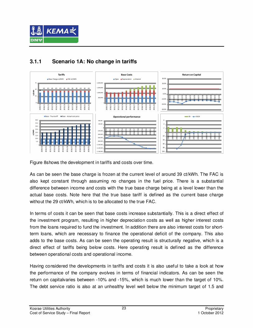
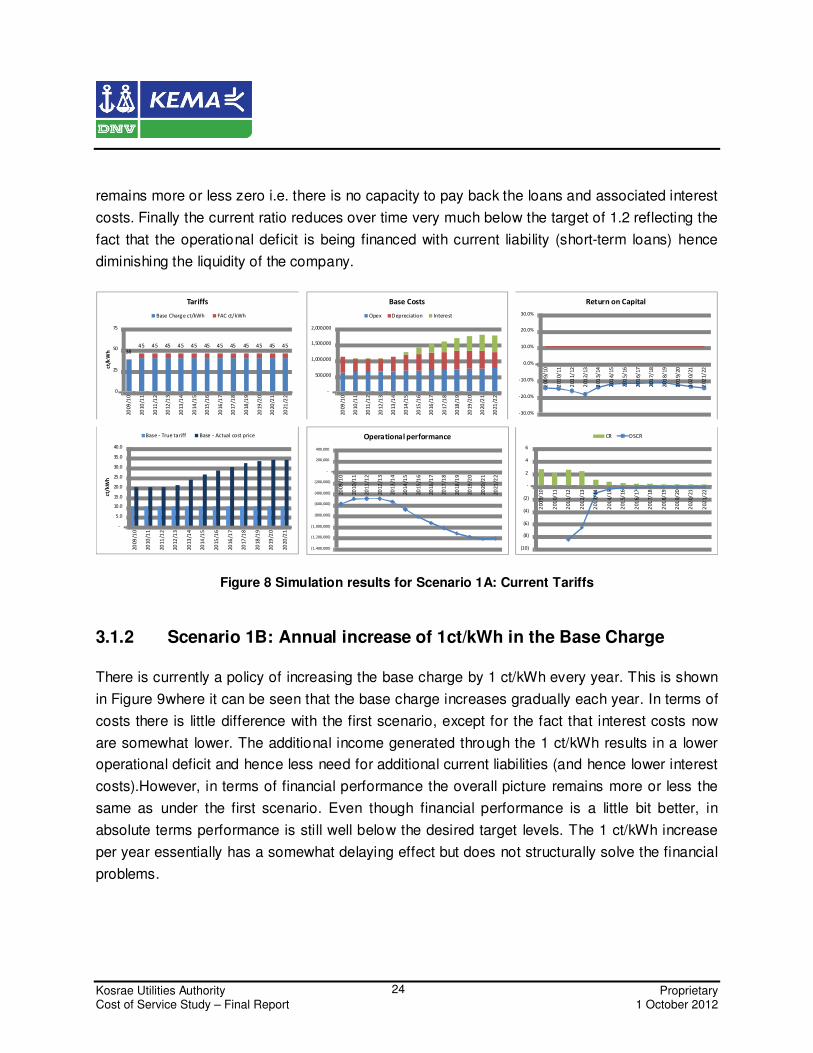
3.1.1 Scenario 1A: No change in tariffs
Figure 8shows the development in tariffs and costs over time.
As can be seen the base charge is frozen at the current level of around 39 ct/kWh. The FAC is
also kept constant through assuming no changes in the fuel price. There is a substantial
difference between income and costs with the true base charge being at a level lower than the
actual base costs. Note here that the true base tariff is defined as the current base charge
without the 29 ct/kWh, which is to be allocated to the true FAC.
In terms of costs it can be seen that base costs increase substantially. This is a direct effect of
the investment program, resulting in higher depreciation costs as well as higher interest costs
from the loans required to fund the investment. In addition there are also interest costs for short-
term loans, which are necessary to finance the operational deficit of the company. This also
adds to the base costs. As can be seen the operating result is structurally negative, which is a
direct effect of tariffs being below costs. Here operating result is defined as the difference
between operational costs and operational income.
Having considered the developments in tariffs and costs it is also useful to take a look at how
the performance of the company evolves in terms of financial indicators. As can be seen the
return on capitalvaries between -10% and -15%, which is much lower than the target of 10%.
The debt service ratio is also at an unhealthy level well below the minimum target of 1.5 and
(10)
(8)
(6)
(4)
(2)
-
2
4
6
20
09
/1
0
20
10
/1
1
20
11
/1
2
20
12
/1
3
20
13
/1
4
20
14
/1
5
20
15
/1
6
20
16
/1
7
20
17
/1
8
20
18
/1
9
20
19
/2
0
20
20
/2
1
20
21
/2
2
CR DSCR
-30.0%
-20.0%
-10.0%
0.0%
10.0%
20.0%
30.0%
20
09
/1
0
20
10
/1
1
20
11
/1
2
20
12
/1
3
20
13
/1
4
20
14
/1
5
20
15
/1
6
20
16
/1
7
20
17
/1
8
20
18
/1
9
20
19
/2
0
20
20
/2
1
20
21
/2
2
Return on Capital
(1,400,000)
(1,200,000)
(1,000,000)
(800,000)
(600,000)
(400,000)
(200,000)
-
200 ,000
400 ,000
20
09
/10
20
10
/11
20
11
/12
20
12
/13
20
13
/14
20
14
/15
20
15
/16
20
16
/17
20
17
/18
20
18
/19
20
19
/20
20
20
/21
20
21
/22
Operational performance
3845 45 45 45 45 45 45 45 45 45 45 45
0
25
50
75
20
09
/10
20
10
/11
20
11
/12
20
12
/13
20
13
/14
20
14
/15
20
15
/16
20
16
/17
20
17
/18
20
18
/19
20
19
/20
20
20
/21
20
21
/22
ct/k
Wh
Tariffs
Base Charge ct/kWh FAC ct/kWh
-
5.0
10.0
15.0
20.0
25.0
30.0
35.0
40.0
20
09
/10
20
10
/11
20
11
/12
20
12
/13
20
13
/14
20
14
/15
20
15
/16
20
16
/17
20
17
/18
20
18
/19
20
19
/20
20
20
/21
ct/
kW
h
Base - True tariff Base - Actual cost price
-
500,000
1,000,000
1,500,000
2,000,000
20
09
/10
20
10
/11
20
11
/12
20
12
/13
20
13
/14
20
14
/15
20
15
/16
20
16
/17
20
17
/18
20
18
/19
20
19
/20
20
20
/21
20
21
/22
Base Costs
Opex Depreciation Interest
Kosrae Utilities Authority Proprietary Cost of Service Study – Final Report 1 October 2012
24
remains more or less zero i.e. there is no capacity to pay back the loans and associated interest
costs. Finally the current ratio reduces over time very much below the target of 1.2 reflecting the
fact that the operational deficit is being financed with current liability (short-term loans) hence
diminishing the liquidity of the company.
Figure 8 Simulation results for Scenario 1A: Current Tariffs
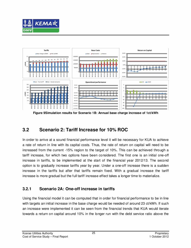
3.1.2 Scenario 1B: Annual increase of 1ct/kWh in the Base Charge
There is currently a policy of increasing the base charge by 1 ct/kWh every year. This is shown
in Figure 9where it can be seen that the base charge increases gradually each year. In terms of
costs there is little difference with the first scenario, except for the fact that interest costs now
are somewhat lower. The additional income generated through the 1 ct/kWh results in a lower
operational deficit and hence less need for additional current liabilities (and hence lower interest
costs).However, in terms of financial performance the overall picture remains more or less the
same as under the first scenario. Even though financial performance is a little bit better, in
absolute terms performance is still well below the desired target levels. The 1 ct/kWh increase
per year essentially has a somewhat delaying effect but does not structurally solve the financial
problems.
(10)
(8)
(6)
(4)
(2)
-
2
4
6
20
09
/1
0
20
10
/1
1
20
11
/1
2
20
12
/1
3
20
13
/1
4
20
14
/1
5
20
15
/1
6
20
16
/1
7
20
17
/1
8
20
18
/1
9
20
19
/2
0
20
20
/2
1
20
21
/2
2
CR DSCR
-30.0%
-20.0%
-10.0%
0.0%
10.0%
20.0%
30.0%
20
09
/1
0
20
10
/1
1
20
11
/1
2
20
12
/1
3
20
13
/1
4
20
14
/1
5
20
15
/1
6
20
16
/1
7
20
17
/1
8
20
18
/1
9
20
19
/2
0
20
20
/2
1
20
21
/2
2
Return on Capital
(1,400,000)
(1,200,000)
(1,000,000)
(800,000)
(600,000)
(400,000)
(200,000)
-
200 ,000
400 ,000
20
09
/10
20
10
/11
20
11
/12
20
12
/13
20
13
/14
20
14
/15
20
15
/16
20
16
/17
20
17
/18
20
18
/19
20
19
/20
20
20
/21
20
21
/22
Operational performance
3845 45 45 45 45 45 45 45 45 45 45 45
0
25
50
75
20
09
/10
20
10
/11
20
11
/12
20
12
/13
20
13
/14
20
14
/15
20
15
/16
20
16
/17
20
17
/18
20
18
/19
20
19
/20
20
20
/21
20
21
/22
ct/k
Wh
Tariffs
Base Charge ct/kWh FAC ct/kWh
-
5.0
10.0
15.0
20.0
25.0
30.0
35.0
40.0
20
09
/10
20
10
/11
20
11
/12
20
12
/13
20
13
/14
20
14
/15
20
15
/16
20
16
/17
20
17
/18
20
18
/19
20
19
/20
20
20
/21
ct/
kW
h
Base - True tariff Base - Actual cost price
-
500,000
1,000,000
1,500,000
2,000,000
20
09
/10
20
10
/11
20
11
/12
20
12
/13
20
13
/14
20
14
/15
20
15
/16
20
16
/17
20
17
/18
20
18
/19
20
19
/20
20
20
/21
20
21
/22
Base Costs
Opex Depreciation Interest
Kosrae Utilities Authority Proprietary Cost of Service Study – Final Report 1 October 2012
25
Figure 9Simulation results for Scenario 1B: Annual base charge increase of 1ct/kWh
3.2 Scenario 2: Tariff Increase for 10% ROC
In order to arrive at a sound financial performance level it will be necessary for KUA to achieve
a rate of return in line with its capital costs. Thus, the rate of return on capital will need to be
increased from the current -15% region to the target of 10%. This can be achieved through a
tariff increase, for which two options have been considered. The first one is an initial one-off
increase in tariffs, to be implemented at the start of the financial year 2012/13. The second
option is to gradually increase tariffs year by year. Under a one-off increase there is a sudden
increase in the tariffs but after that tariffs remain fixed. With a gradual increase the tariff
increase is more gradual but the full tariff increase effect takes a longer time to materialize.
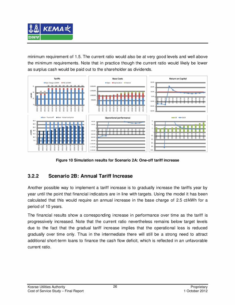
3.2.1 Scenario 2A: One-off increase in tariffs
Using the financial model it can be computed that in order for financial performance to be in line
with targets an initial increase in the base charge would be needed of around 23 ct/kWh. If such
an increase were implemented it can be seen from the financial trends that KUA would iterate
towards a return on capital around 10% in the longer run with the debt service ratio above the
(10)
(8)
(6)
(4)
(2)
-
2
4
6
20
09
/1
0
20
10
/1
1
20
11
/1
2
20
12
/1
3
20
13
/1
4
20
14
/1
5
20
15
/1
6
20
16
/1
7
20
17
/1
8
20
18
/1
9
20
19
/2
0
20
20
/2
1
20
21
/2
2
CR DSCR
-30.0%
-20.0%
-10.0%
0.0%
10.0%
20.0%
30.0%
20
09
/1
0
20
10
/1
1
20
11
/1
2
20
12
/1
3
20
13
/1
4
20
14
/1
5
20
15
/1
6
20
16
/1
7
20
17
/1
8
20
18
/1
9
20
19
/2
0
20
20
/2
1
20
21
/2
2
Return on Capital
(1,400,000)
(1,200,000)
(1,000,000)
(800,000)
(600,000)
(400,000)
(200,000)
-
200 ,000
400 ,000
20
09
/10
20
10
/11
20
11
/12
20
12
/13
20
13
/14
20
14
/15
20
15
/16
20
16
/17
20
17
/18
20
18
/19
20
19
/20
20
20
/21
20
21
/22
Operational performance
3845 45 46 47 48 49 50 51 52 53 54 55
0
25
50
75
20
09
/10
20
10
/11
20
11
/12
20
12
/13
20
13
/14
20
14
/15
20
15
/16
20
16
/17
20
17
/18
20
18
/19
20
19
/20
20
20
/21
20
21
/22
ct/k
Wh
Tariffs
Base Charge ct/kWh FAC ct/kWh
-
5.0
10.0
15.0
20.0
25.0
30.0
35.0
20
09
/10
20
10
/11
20
11
/12
20
12
/13
20
13
/14
20
14
/15
20
15
/16
20
16
/17
20
17
/18
20
18
/19
20
19
/20
20
20
/21
ct/
kW
h
Base - True tariff Base - Actual cost price
-
500,000
1,000,000
1,500,000
2,000,000
20
09
/10
20
10
/11
20
11
/12
20
12
/13
20
13
/14
20
14
/15
20
15
/16
20
16
/17
20
17
/18
20
18
/19
20
19
/20
20
20
/21
20
21
/22
Base Costs
Opex Depreciation Interest
Kosrae Utilities Authority Proprietary Cost of Service Study – Final Report 1 October 2012
26
minimum requirement of 1.5. The current ratio would also be at very good levels and well above
the minimum requirements. Note that in practice though the current ratio would likely be lower
as surplus cash would be paid out to the shareholder as dividends.
Figure 10 Simulation results for Scenario 2A: One-off tariff increase
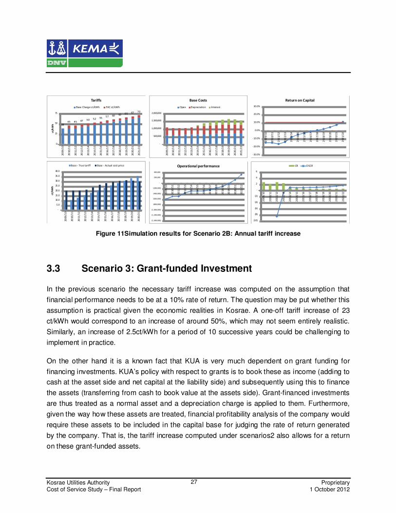
3.2.2 Scenario 2B: Annual Tariff Increase
Another possible way to implement a tariff increase is to gradually increase the tariffs year by
year until the point that financial indicators are in line with targets. Using the model it has been
calculated that this would require an annual increase in the base charge of 2.5 ct/kWh for a
period of 10 years.
The financial results show a corresponding increase in performance over time as the tariff is
progressively increased. Note that the current ratio nevertheless remains below target levels
due to the fact that the gradual tariff increase implies that the operational loss is reduced
gradually over time only. Thus in the intermediate there will still be a strong need to attract
additional short-term loans to finance the cash flow deficit, which is reflected in an unfavorable
current ratio.
(10)
(8)
(6)
(4)
(2)
-
2
4
6
20
09
/1
0
20
10
/1
1
20
11
/1
2
20
12
/1
3
20
13
/1
4
20
14
/1
5
20
15
/1
6
20
16
/1
7
20
17
/1
8
20
18
/1
9
20
19
/2
0
20
20
/2
1
20
21
/2
2
CR DSCR
-30.0%
-20.0%
-10.0%
0.0%
10.0%
20.0%
30.0%
20
09
/1
0
20
10
/1
1
20
11
/1
2
20
12
/1
3
20
13
/1
4
20
14
/1
5
20
15
/1
6
20
16
/1
7
20
17
/1
8
20
18
/1
9
20
19
/2
0
20
20
/2
1
20
21
/2
2
Return on Capital
(1,400,000)
(1,200,000)
(1,000,000)
(800,000)
(600,000)
(400,000)
(200,000)
-
200 ,000
400 ,000
20
09
/10
20
10
/11
20
11
/12
20
12
/13
20
13
/14
20
14
/15
20
15
/16
20
16
/17
20
17
/18
20
18
/19
20
19
/20
20
20
/21
20
21
/22
Operational performance
3845 45
68 68 68 68 68 68 68 68 68 68
0
25
50
75
20
09
/10
20
10
/11
20
11
/12
20
12
/13
20
13
/14
20
14
/15
20
15
/16
20
16
/17
20
17
/18
20
18
/19
20
19
/20
20
20
/21
20
21
/22
ct/k
Wh
Tariffs
Base Charge ct/kWh FAC ct/kWh
-
5.0
10.0
15.0
20.0
25.0
30.0
35.0
20
09
/10
20
10
/11
20
11
/12
20
12
/13
20
13
/14
20
14
/15
20
15
/16
20
16
/17
20
17
/18
20
18
/19
20
19
/20
20
20
/21
ct/
kW
h
Base - True tariff Base - Actual cost price
-
500,000
1,000,000
1,500,000
2,000,000
20
09
/10
20
10
/11
20
11
/12
20
12
/13
20
13
/14
20
14
/15
20
15
/16
20
16
/17
20
17
/18
20
18
/19
20
19
/20
20
20
/21
20
21
/22
Base Costs
Opex Depreciation Interest
Kosrae Utilities Authority Proprietary Cost of Service Study – Final Report 1 October 2012
27
Figure 11Simulation results for Scenario 2B: Annual tariff increase
3.3 Scenario 3: Grant-funded Investment
In the previous scenario the necessary tariff increase was computed on the assumption that
financial performance needs to be at a 10% rate of return. The question may be put whether this
assumption is practical given the economic realities in Kosrae. A one-off tariff increase of 23
ct/kWh would correspond to an increase of around 50%, which may not seem entirely realistic.
Similarly, an increase of 2.5ct/kWh for a period of 10 successive years could be challenging to
implement in practice.
On the other hand it is a known fact that KUA is very much dependent on grant funding for
financing investments. KUA’s policy with respect to grants is to book these as income (adding to
cash at the asset side and net capital at the liability side) and subsequently using this to finance
the assets (transferring from cash to book value at the assets side). Grant-financed investments
are thus treated as a normal asset and a depreciation charge is applied to them. Furthermore,
given the way how these assets are treated, financial profitability analysis of the company would
require these assets to be included in the capital base for judging the rate of return generated
by the company. That is, the tariff increase computed under scenarios2 also allows for a return
on these grant-funded assets.
(10)
(8)
(6)
(4)
(2)
-
2
4
6
20
09
/1
0
20
10
/1
1
20
11
/1
2
20
12
/1
3
20
13
/1
4
20
14
/1
5
20
15
/1
6
20
16
/1
7
20
17
/1
8
20
18
/1
9
20
19
/2
0
20
20
/2
1
20
21
/2
2
CR DSCR
-30.0%
-20.0%
-10.0%
0.0%
10.0%
20.0%
30.0%
20
09
/1
0
20
10
/1
1
20
11
/1
2
20
12
/1
3
20
13
/1
4
20
14
/1
5
20
15
/1
6
20
16
/1
7
20
17
/1
8
20
18
/1
9
20
19
/2
0
20
20
/2
1
20
21
/2
2
Return on Capital
(1,400,000)
(1,200,000)
(1,000,000)
(800,000)
(600,000)
(400,000)
(200,000)
-
200 ,000
400 ,000
20
09
/10
20
10
/11
20
11
/12
20
12
/13
20
13
/14
20
14
/15
20
15
/16
20
16
/17
20
17
/18
20
18
/19
20
19
/20
20
20
/21
20
21
/22
Operational performance
3845 45 47 50 52 55
57 60 62 65 67 70
0
25
50
75
20
09
/10
20
10
/11
20
11
/12
20
12
/13
20
13
/14
20
14
/15
20
15
/16
20
16
/17
20
17
/18
20
18
/19
20
19
/20
20
20
/21
20
21
/22
ct/k
Wh
Tariffs
Base Charge ct/kWh FAC ct/kWh
-
5.0
10.0
15.0
20.0
25.0
30.0
35.0
40.0
20
09
/10
20
10
/11
20
11
/12
20
12
/13
20
13
/14
20
14
/15
20
15
/16
20
16
/17
20
17
/18
20
18
/19
20
19
/20
20
20
/21
ct/
kW
h
Base - True tariff Base - Actual cost price
-
500,000
1,000,000
1,500,000
2,000,000
20
09
/10
20
10
/11
20
11
/12
20
12
/13
20
13
/14
20
14
/15
20
15
/16
20
16
/17
20
17
/18
20
18
/19
20
19
/20
20
20
/21
20
21
/22
Base Costs
Opex Depreciation Interest

Kosrae Utilities Authority Proprietary Cost of Service Study – Final Report 1 October 2012
28
Theoretically speaking such a return should be applied as it represents a return on the
company’s capital. Thus, the company could have used the grant alternatively and earned a
return on that investment. Not allowing for a return would thus imply opportunity costs. In
practice however the grant is most likely to be conditional on specific investments and
alternative applications of the grant amounts are typically not allowed. Then the grant becomes
sunk and making allowances for a return would no longer be justified.
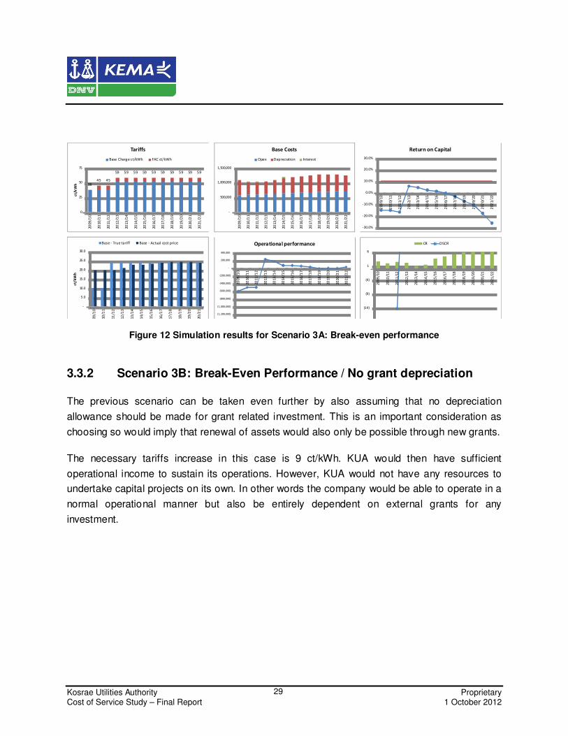
3.3.1 Scenario 3A: Break-Even Performance
In this light an alternative scenario has been analyzed where the assumption is that future
investment is funded through grants. Furthermore the assumption is that no return is expected
on these investments. This means that under this scenario KUA is expected to achieve a break-
even outcome with operational income at the same level as operational expenditures. There
would be no costs of capital as all capital is financed through grants.
Note that in the operational expenditures an allowance for depreciation on grant-funded assets
is included here. This assumes that KUA should make sufficient reservations to be able to
replace these assets at the end of their lifetime through own funds rather than being dependent
on grants again.
The break-even situation is expected to be achieved through a one-off increase of the tariff.This
increase is calculated to be 14 ct/kWh. Note that in the initial year there would be an operational
surplus but in subsequent years the tariffs and costs would align again with increasing costs
over time.
Kosrae Utilities Authority Proprietary Cost of Service Study – Final Report 1 October 2012
29
Figure 12 Simulation results for Scenario 3A: Break-even performance
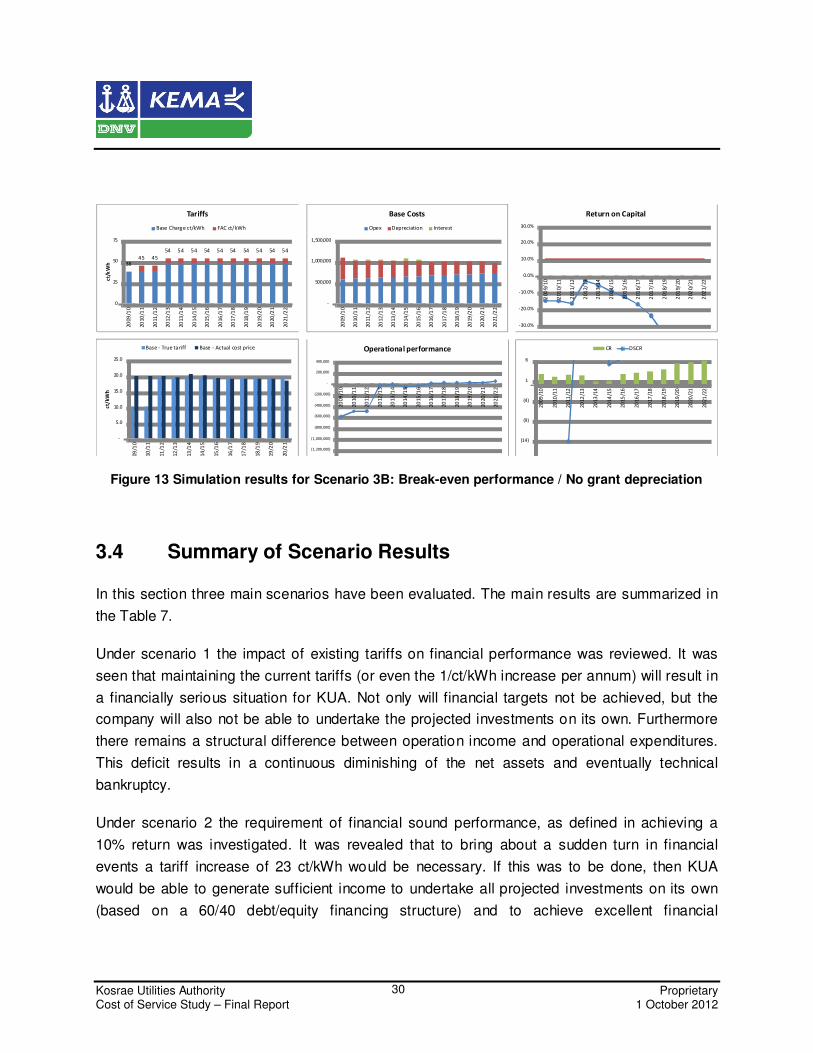
3.3.2 Scenario 3B: Break-Even Performance / No grant depreciation
The previous scenario can be taken even further by also assuming that no depreciation
allowance should be made for grant related investment. This is an important consideration as
choosing so would imply that renewal of assets would also only be possible through new grants.
The necessary tariffs increase in this case is 9 ct/kWh. KUA would then have sufficient
operational income to sustain its operations. However, KUA would not have any resources to
undertake capital projects on its own. In other words the company would be able to operate in a
normal operational manner but also be entirely dependent on external grants for any
investment.
(14)
(9)
(4)
1
6
20
09
/10
20
10
/11
20
11
/12
20
12
/13
20
13
/14
20
14
/15
20
15
/16
20
16
/17
20
17
/18
20
18
/19
20
19
/20
20
20
/21
20
21
/22
CR DSCR
-30.0%
-20.0%
-10.0%
0.0%
10.0%
20.0%
30.0%
20
09
/1
0
20
10
/1
1
20
11
/1
2
20
12
/1
3
20
13
/1
4
20
14
/1
5
20
15
/1
6
20
16
/1
7
20
17
/1
8
20
18
/1
9
20
19
/2
0
20
20
/2
1
20
21
/2
2
Return on Capital
(1,200,000)
(1,000,000)
(800,000)
(600,000)
(400,000)
(200,000)
-
200 ,000
400 ,000
20
09
/10
20
10
/11
20
11
/12
20
12
/13
20
13
/14
20
14
/15
20
15
/16
20
16
/17
20
17
/18
20
18
/19
20
19
/20
20
20
/21
20
21
/22
Operational performance
3845 45
59 59 59 59 59 59 59 59 59 59
0
25
50
75
20
09
/10
20
10
/11
20
11
/12
20
12
/13
20
13
/14
20
14
/15
20
15
/16
20
16
/17
20
17
/18
20
18
/19
20
19
/20
20
20
/21
20
21
/22
ct/k
Wh
Tariffs
Base Charge ct/kWh FAC ct/kWh
-
5.0
10.0
15.0
20.0
25.0
30.0
20
09
/10
20
10
/11
20
11
/12
20
12
/13
20
13
/14
20
14
/15
20
15
/16
20
16
/17
20
17
/18
20
18
/19
20
19
/20
20
20
/21
ct/
kW
h
Base - True tariff Base - Actual cost price
-
500,000
1,000,000
1,500,000
20
09
/10
20
10
/11
20
11
/12
20
12
/13
20
13
/14
20
14
/15
20
15
/16
20
16
/17
20
17
/18
20
18
/19
20
19
/20
20
20
/21
20
21
/22
Base Costs
Opex Depreciation Interest
Kosrae Utilities Authority Proprietary Cost of Service Study – Final Report 1 October 2012
30
Figure 13 Simulation results for Scenario 3B: Break-even performance / No grant depreciation
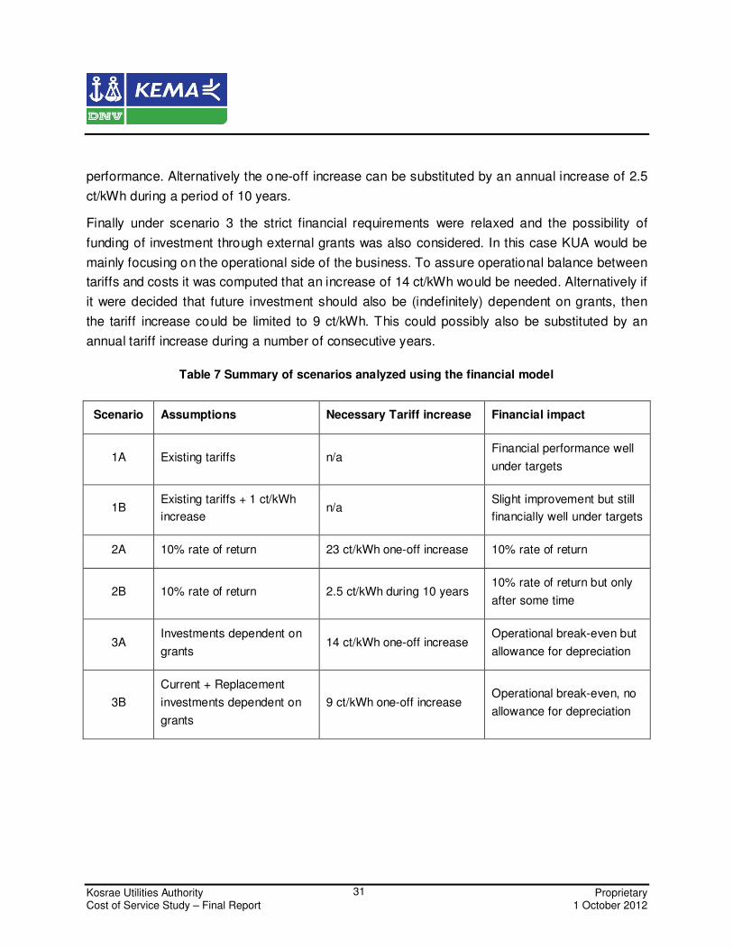
3.4 Summary of Scenario Results
In this section three main scenarios have been evaluated. The main results are summarized in
the Table 7.
Under scenario 1 the impact of existing tariffs on financial performance was reviewed. It was
seen that maintaining the current tariffs (or even the 1/ct/kWh increase per annum) will result in
a financially serious situation for KUA. Not only will financial targets not be achieved, but the
company will also not be able to undertake the projected investments on its own. Furthermore
there remains a structural difference between operation income and operational expenditures.
This deficit results in a continuous diminishing of the net assets and eventually technical
bankruptcy.
Under scenario 2 the requirement of financial sound performance, as defined in achieving a
10% return was investigated. It was revealed that to bring about a sudden turn in financial
events a tariff increase of 23 ct/kWh would be necessary. If this was to be done, then KUA
would be able to generate sufficient income to undertake all projected investments on its own
(based on a 60/40 debt/equity financing structure) and to achieve excellent financial
(14)
(9)
(4)
1
6
20
09
/10
20
10
/11
20
11
/12
20
12
/13
20
13
/14
20
14
/15
20
15
/16
20
16
/17
20
17
/18
20
18
/19
20
19
/20
20
20
/21
20
21
/22
CR DSCR
-30.0%
-20.0%
-10.0%
0.0%
10.0%
20.0%
30.0%
20
09
/1
0
20
10
/1
1
20
11
/1
2
20
12
/1
3
20
13
/1
4
20
14
/1
5
20
15
/1
6
20
16
/1
7
20
17
/1
8
20
18
/1
9
20
19
/2
0
20
20
/2
1
20
21
/2
2
Return on Capital
(1,200,000)
(1,000,000)
(800,000)
(600,000)
(400,000)
(200,000)
-
200 ,000
400 ,000
20
09
/10
20
10
/11
20
11
/12
20
12
/13
20
13
/14
20
14
/15
20
15
/16
20
16
/17
20
17
/18
20
18
/19
20
19
/20
20
20
/21
20
21
/22
Operational performance
3845 45
54 54 54 54 54 54 54 54 54 54
0
25
50
75
20
09
/10
20
10
/11
20
11
/12
20
12
/13
20
13
/14
20
14
/15
20
15
/16
20
16
/17
20
17
/18
20
18
/19
20
19
/20
20
20
/21
20
21
/22
ct/k
Wh
Tariffs
Base Charge ct/kWh FAC ct/kWh
-
5.0
10.0
15.0
20.0
25.0
20
09
/10
20
10
/11
20
11
/12
20
12
/13
20
13
/14
20
14
/15
20
15
/16
20
16
/17
20
17
/18
20
18
/19
20
19
/20
20
20
/21
ct/
kW
h
Base - True tariff Base - Actual cost price
-
500,000
1,000,000
1,500,000
20
09
/10
20
10
/11
20
11
/12
20
12
/13
20
13
/14
20
14
/15
20
15
/16
20
16
/17
20
17
/18
20
18
/19
20
19
/20
20
20
/21
20
21
/22
Base Costs
Opex Depreciation Interest
Kosrae Utilities Authority Proprietary Cost of Service Study – Final Report 1 October 2012
31
performance. Alternatively the one-off increase can be substituted by an annual increase of 2.5
ct/kWh during a period of 10 years.
Finally under scenario 3 the strict financial requirements were relaxed and the possibility of
funding of investment through external grants was also considered. In this case KUA would be
mainly focusing on the operational side of the business. To assure operational balance between
tariffs and costs it was computed that an increase of 14 ct/kWh would be needed. Alternatively if
it were decided that future investment should also be (indefinitely) dependent on grants, then
the tariff increase could be limited to 9 ct/kWh. This could possibly also be substituted by an
annual tariff increase during a number of consecutive years.
Table 7 Summary of scenarios analyzed using the financial model
Scenario Assumptions Necessary Tariff increase Financial impact
1A Existing tariffs n/a Financial performance well
under targets
1B Existing tariffs + 1 ct/kWh
increase n/a
Slight improvement but still
financially well under targets
2A 10% rate of return 23 ct/kWh one-off increase 10% rate of return
2B 10% rate of return 2.5 ct/kWh during 10 years 10% rate of return but only
after some time
3A Investments dependent on
grants 14 ct/kWh one-off increase
Operational break-even but
allowance for depreciation
3B
Current + Replacement
investments dependent on
grants
9 ct/kWh one-off increase Operational break-even, no
allowance for depreciation
Kosrae Utilities Authority Proprietary Cost of Service Study – Final Report 1 October 2012
32
4 Analysis of KUA Tariff Structure
4.1 Cost Allocation Analysis
4.1.1 Introduction
This chapter presents the results of the cost allocation analysis that was carried out for KUA.
The main purpose of this is to obtain information about the true costs per customer group as
compared to the currently implied costs by the existing tariff structure.
The purpose of the cost allocation analysis is to identify to what extent certain customer groups
contribute to the costs of KUA. From a theoretical economic point of view tariffs should be set at
a level such that they reflect the marginal cost of supply. That is, the price paid for each
additional unit of consumption should be equal to the additional costs incurred by the utility due
to the additional consumption. This results in an economically efficient income as customers are
provided with the right price signals.
In practice this marginal cost analysis approach however is not possible to be applied here due
lack of data (absence of demand growth) and the small size of KUA. Due to this it was agreed
that the cost allocation analysis would be based on the so-called embedded cost analysis. Here,
rather than marginal costs we consider the already incurred costs with the company, and try to
allocate these costs to the various customer groups.
In carrying out the cost allocation analysis three steps need to be carried out namely (1)
Functionalization, (2) Cost Classification, and (3) Allocation to Customers. These are discussed
in the following sections.

Kosrae Utilities Authority Proprietary Cost of Service Study – Final Report 1 October 2012
33
4.1.2 Functionalization
First the three main functions within the electricity supply chain need to be identified namely (1)
Generation, (2) Network, and (3) Supply:
• Generation costs are related to the function of producing the electricity; this would entail
the costs associated with the power plant (including station/auxiliary losses).
• Network costs are those costs incurred in the network system (note that KUA only has
distribution and no transmission) and would include the costs associated with the
investment and maintenance of these assets as well as the technical and non-technical
losses.
• Supply costs are those costs not associated with the technical product (electricity) but
the costs associated with metering and billing and service to customers.
For carrying out the cost functionalization use was made of cost data from KUA’s accounting
systems. In this system the costs are allocated to the following cost centers:
1. ADM: Administration
2. CSM: Customer service and metering
3. DST: Distribution
4. PRO: Production
5. P&E: Planning and engineering
The five cost centers have been rearranged into the three functions (Generation, Network,
Supply) based on the following criteria:
• Cost of DST and PRO are directly allocated to Network and Generation, respectively;
• Cost of CST has been allocated to Supply;
• Costs of ADM have been allocated to the three functions on a pro rata basis;
Kosrae Utilities Authority Proprietary Cost of Service Study – Final Report 1 October 2012
34
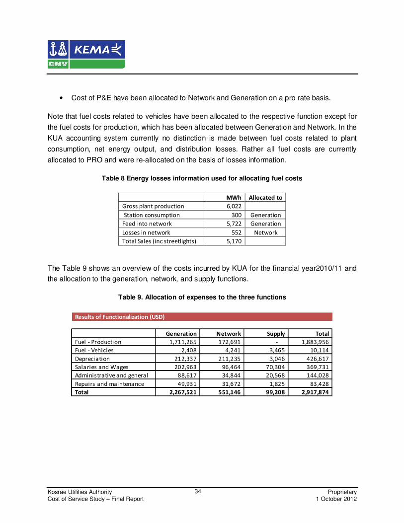
• Cost of P&E have been allocated to Network and Generation on a pro rate basis.
Note that fuel costs related to vehicles have been allocated to the respective function except for
the fuel costs for production, which has been allocated between Generation and Network. In the
KUA accounting system currently no distinction is made between fuel costs related to plant
consumption, net energy output, and distribution losses. Rather all fuel costs are currently
allocated to PRO and were re-allocated on the basis of losses information.
Table 8 Energy losses information used for allocating fuel costs
MWh Allocated to
Gross plant production 6,022
Station consumption 300 Generation
Feed into network 5,722 Generation
Losses in network 552 Network
Total Sales (inc streetlights) 5,170
The Table 9 shows an overview of the costs incurred by KUA for the financial year2010/11 and
the allocation to the generation, network, and supply functions.
Table 9. Allocation of expenses to the three functions
Results of Functionalization (USD)
Generation Network Supply Total
Fuel - Production 1,711,265 172,691 - 1,883,956
Fuel - Vehicles 2,408 4,241 3,465 10,114
Depreciation 212,337 211,235 3,046 426,617
Salaries and Wages 202,963 96,464 70,304 369,731
Administrative and general 88,617 34,844 20,568 144,028
Repairs and maintenance 49,931 31,672 1,825 83,428
Total 2,267,521 551,146 99,208 2,917,874

Kosrae Utilities Authority Proprietary Cost of Service Study – Final Report 1 October 2012
35
4.1.3 Classification
The next step is to classify the costs identified under the functionalization step into different cost
components. These represent the services supplied by KUA which, in principle, should also be
charged for as separate “products”:
• Capacity Component (kVA): These represent the costs incurred by KUA related to
provide a system capable of meeting all capacity requested by its customers. Simply
stated these are the costs of setting up and maintaining a system such that the potential
demand of all customers could be satisfied. These costs are fixed costs i.e. do not
change as a function of consumption (in the short-term at least).
• Energy Component (kWh): Energy costs vary directly with kWh production and are
mainly related to the fuel and associated costs. Notably these costs are not only driven
by consumption but also the level of losses i.e. the network losses and station
consumption.
• Connection Component: These costs vary as a function of the number customers and
include costs associated with providing the connection i.e. customer services, metering,
and billing.
For the allocation all fuel related costs have been allocated to the energy component while all
other costs are allocated to the demand component. For supply, all costs are allocated to the
customer component. The Table 10 shows the result of this allocation.
Table 10. Allocation of costs to demand, energy, and customer components
The interpretation of the classification table should be that KUA is incurring costs in three areas
(generation, network, supply) while providing three types of services (capacity, energy,
Results of Classification (USD)
Capacity Energy Connection Total
Generation 556,255 1,711,265 - 2,267,521
Network 378,455 172,691 - 551,146
Supply - - 99,208 99,208
Total 934,710 1,883,956 99,208 2,917,874

Kosrae Utilities Authority Proprietary Cost of Service Study – Final Report 1 October 2012
36
connection) to its customers. In principle each of these three services should be priced
separately with customers paying:
• A fee for capacity based on the size of their connection (kVA)
• A fee for energy based on their actual consumption (kWh)
• A fee for connection based on the number of connections (#)
4.1.4 Allocation
4.1.4.1 Determination of allocation factors
The final step is to allocate the costs identified above to the various customer categories. The
basis on which allocation is to take place per product isshown inTable 11.
Table 11. Allocation basis per customer category
Allocation of energy and connection costs can be done on the basis of energy sales and
number of customers, respectively. For the allocation of capacity costs the peak demand for the
particular customer group is generally used. In this case the non-coincidental peak has been
used. Demand information at the level of customer categories is currently not being collected
within KUA and therefore had to be synthesized. The process followed for this is explained next.
Allocation Factors
Allocation of: Capacity Energy Connection
Allocation basis:
Non-
Coincidental
Peak (kW)
Sales (kWh)Nr of
Customers
Residential 597 2,015,675 1,458
Commercial 245 1,424,550 246
Government 153 889,943 82
Non-Government 77 446,874 69
Industrial 54 311,349 15
Total 1,125 5,088,390 1,870
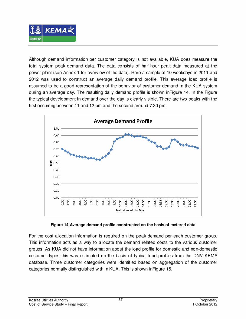
Kosrae Utilities Authority Proprietary Cost of Service Study – Final Report 1 October 2012
37
Although demand information per customer category is not available, KUA does measure the
total system peak demand data. The data consists of half-hour peak data measured at the
power plant (see Annex 1 for overview of the data). Here a sample of 10 weekdays in 2011 and
2012 was used to construct an average daily demand profile. This average load profile is
assumed to be a good representation of the behavior of customer demand in the KUA system
during an average day. The resulting daily demand profile is shown inFigure 14. In the Figure
the typical development in demand over the day is clearly visible. There are two peaks with the
first occurring between 11 and 12 pm and the second around 7:30 pm.
Figure 14 Average demand profile constructed on the basis of metered data
For the cost allocation information is required on the peak demand per each customer group.
This information acts as a way to allocate the demand related costs to the various customer
groups. As KUA did not have information about the load profile for domestic and non-domestic
customer types this was estimated on the basis of typical load profiles from the DNV KEMA
database. Three customer categories were identified based on aggregation of the customer
categories normally distinguished with in KUA. This is shown inFigure 15.

Kosrae Utilities Authority Proprietary Cost of Service Study – Final Report 1 October 2012
38
Figure 15 Allocation applied in estimation of demand profiles
The government, commercial and non-government categories were aggregated into a single
category (non-domestic) as it would not appear possible to derive accurate load curves for each
category separately. At the same time it seems that these categories tend to have more or less
the same demand pattern during the day which closely resembles a commercial demand profile.
For domestic and non-domestic typical load profiles from the DNV KEMA database were used
as a starting point. For yard lights the load profile used was based on the known information that
lights are turned on between 6 pm and 6 am i.e. a load factor of 50%.
The standard load profiles together with the yard light profile were aligned with the actual load
data in two steps. First by fine-tuning the standard load profiles to bring these in line with the
demand times as observed in the KUA system. This involved the horizontal shifting and
compression of the typical demand curves to match the normal times observed in Kosrae with
regard to sun-rise, sun-set, and working hours. The second step was to vertically align the
demand profiles to assure that total actual measured demand matches the synthesized demand
as much as possible. This was done through the minimization of the quadratic difference
between the actual demand curve and the synthesized demand curve.
Figure 16 shows the resulting match between the average load profile and the synthesized load
profile. As can be seen there are some differences due to errors in the estimation but generally
there is a good match between projected and actual profile the total deviation being slightly

Kosrae Utilities Authority Proprietary Cost of Service Study – Final Report 1 October 2012
39
more than 1%. From the load profile information the non-coincidental peak demand for each
customer class was finally derived, as shown in Table 11.
Figure 16. Match between the average demand profile based on metered data and the constructed
profile using the synthesized load profiles per customer class.
4.1.4.2 Allocation to Customer Categories
The information regarding sales and quantities can be used to perform the allocation from the
cost classification towards the customer classes. This computation isshown inTable 12. Here,
each cost category is allocated to each customer class whereby allocations are done on the
basis of the non-coincidental peak, total sales, and number of customers for respectively the
demand costs, energy costs, and customer costs.

Kosrae Utilities Authority Proprietary Cost of Service Study – Final Report 1 October 2012
40
Table 12. Cost allocation results
Finally the costs can be allocated to the various customer categories by summing up the
respective costs per generation, network, and supply components. The results areshown
inTable 13. As can be seen the costs of residential customers are around 65.5 ct/kWh, which is
about 25% higher than the other categories, whose costs are around 51 to 52 ct/kWh. This can
be explained by the less favorable demand profile for these customers. This is in line with what
is generally observed elsewhere. Note further that the costs for the other customer categories
are very similar. In larger power systems one would tend to notice more variation in costs. In the
KUA system however the customers are much more homogenous in terms of demand profile
and hence also tend to have similar costs per kWh.
Table 13. Final results
Demand Energy Customer
Generation Resi dential 295,167 677,887 -
Commerci al 121,044 479,087 -
Government 75,618 299,295 -
Non-Government 37,971 150,287 -
Industrial 26,455 104,709 -
Network Resi dential 200,820 68,408 -
Commerci al 82,354 48,347 -
Government 51,448 30,203 -
Non-Government 25,834 15,166 -
Industrial 17,999 10,567 -
Supply Resi dential - - 77,350
Commerci al - - 13,051
Government - - 4,350
Non-Government - - 3,661
Industrial - - 796
Result of Allocation (USD)
Demand Energy Customer Price (ct/kWh)
Residential 495,987 746,295 77,350 65.5
Commercial 203,397 527,434 13,051 52.2
Government 127,066 329,498 4,350 51.8
Non-Government 63,805 165,453 3,661 52.1
Industrial 44,454 115,276 796 51.6
Total 934,710 1,883,956 99,208
Final Results (USD)
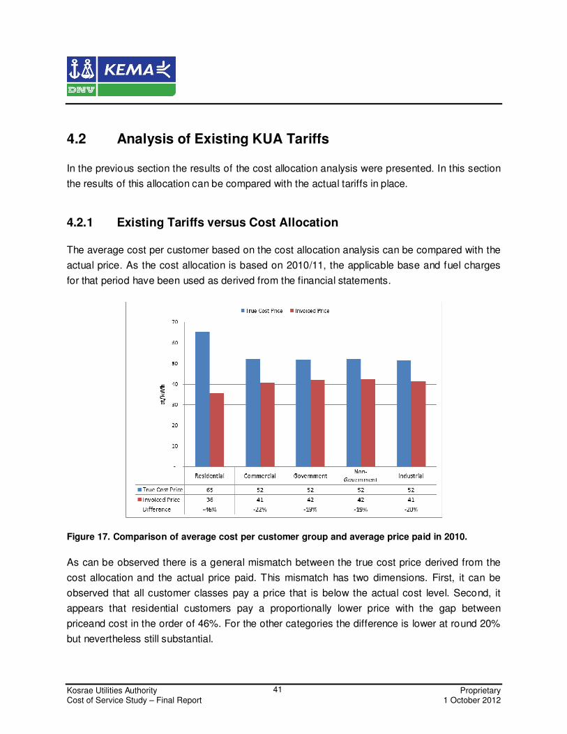
Kosrae Utilities Authority Proprietary Cost of Service Study – Final Report 1 October 2012
41
4.2 Analysis of Existing KUA Tariffs
In the previous section the results of the cost allocation analysis were presented. In this section
the results of this allocation can be compared with the actual tariffs in place.
4.2.1 Existing Tariffs versus Cost Allocation
The average cost per customer based on the cost allocation analysis can be compared with the
actual price. As the cost allocation is based on 2010/11, the applicable base and fuel charges
for that period have been used as derived from the financial statements.
Figure 17. Comparison of average cost per customer group and average price paid in 2010.
As can be observed there is a general mismatch between the true cost price derived from the
cost allocation and the actual price paid. This mismatch has two dimensions. First, it can be
observed that all customer classes pay a price that is below the actual cost level. Second, it
appears that residential customers pay a proportionally lower price with the gap between
priceand cost in the order of 46%. For the other categories the difference is lower at round 20%
but nevertheless still substantial.
Kosrae Utilities Authority Proprietary Cost of Service Study – Final Report 1 October 2012
42
4.2.2 Progressive structure of Tariffs
The cost allocation analysis shows that the existing tariff structure seems to have the intention
for domestic customers to be subsidized by the other groups. However, overall the price level is
well below the actual costs for all customer groups with all groups paying a price lower than it
should be from a cost perspective.
4.2.3 Absence of Demand Tariff
Another observation to be made is that the current tariff structure of KUA consists only of kWh
charges. That is, there are no fixed or demand fees e.g. in terms of a fixed amount per month or
per kVA of connected capacity. As was observedin the cost allocation analysis there are
considerable demand related costs, which are more or less fixed in the short term. Given that
KUA’s income only varies with kWh sales, this creates risks to KUA as there is a mismatch
between costs and income. Demand can be influenced by different factors but most importantly
by fluctuations in the fuel price. Higher fuel prices will tend to reduce demand and therefore
income for KUA. In particular taking into account the recent uncertainty regarding oil prices this
issue is very important to consider.
A more elaborate tariff structure containing fixed and demand related fees can help to deal with
this issue. At the same time, such a structure will also create reallocations in the average price
per customer. In particular for customers with relatively low consumption the introduction of a
fixed tariff will lead to a relatively high increase in the electricity bill. The trade-off between the
reduction in financial risks and possible adverse socio-economic aspects should therefore be
considered in the design of a new tariff structure.
4.2.4 Introduction of renewable sources
The issue of renewable (non-diesel) generating options is currently being considered by KUA. In
this light it should be noted that the current formulation of the FAC does not allow the integration
of non-diesel related production costs to be included into it. The FAC formula explicitly refers to
“diesel fuel price” and the price for such fuel, while it is true that the costs of alternative energy
sources i.e. renewables would not vary with the diesel fuel price. There would thus be a
Kosrae Utilities Authority Proprietary Cost of Service Study – Final Report 1 October 2012
43
discrepancy between the applicable FAC and the actual energy costs (being the sum of diesel
and non-diesel generation).
In the case that the costs of renewables would be below the costs of diesel, the FAC could
potentially act as a mechanism to offset the tariff deficit that KUA is currently facing. In this case,
the FAC would still be set on the basis of the diesel gallon price, but the actual underlying costs
would be lower. This approach however is not recommendable as it will not be transparent and
result in potential confusion at the side of customers. Furthermore the absence of a causal link
between tariffs and costs can lead to adverse effects in case that diesel prices increase or
decrease substantially.
The current formulation of the FAC does not allow renewable energy costs to be incorporated.
At the same time inclusion of (renewable) energy purchase costs is desired and these costs
should be reflected in the tariff structure. There are two main ways to do this depending on the
variability in costs. If the costs of purchased energy are more or less fixed and do not change
over time, this could be could be considered part of the base charge. The disadvantage of this
would be that if in future renewable costs were to be changed (either increased or decreased)
then this would need to be reflected in the base charge, which is less flexible to change as
opposed to the FAC.
If costs of purchased energy tend to fluctuate then they could be recouped through a separate
charge (e.g. Renewable Energy Charge). A more practical solution however is to combine the
costs of fuel and renewable energy into one single Energy Charge. In this case the energy
charge would vary periodically as a function of diesel prices but this change would be
dampened due to the inclusion of the renewable energy (purchase) costs.
4.3 Development of Alternative Tariff Structure
The previous analysis showed two main issues with the current KUA tariffs. First, the financial
analysis revealed that current tariff income levels are insufficient to allow KUA to achieve
financial adequate performance in either the sense of earning a return on investment as well as
to be operationally break even. Second, the cost analysis showed that there is a discrepancy
between the tariff level per customer group and the true costs that should be allocated to that
group.

Kosrae Utilities Authority Proprietary Cost of Service Study – Final Report 1 October 2012
44
4.3.1 Base Charge
The base charge reflects the operational costs of the company (i.e. excluding fuel and
renewable energy costs) and is fixed for a predefined period of time (e.g. 5 years).Base costs
are more or less fixed and are therefore to be recouped through a fixed charge i.e. a charge that
does not vary as a function of actual consumption. This amount should in principle be related to
the connected capacity of the customer (i.e. kVA based). Due to the small scale of the customer
base it would seem more practical however to introduce a fixed amount per month, defined in
absolute dollar terms rather than per installed kVA. Furthermore the customer costs, which are
also fixed, could be incorporated into the same charge.
Based on the findings from the cost allocation analysis presented in the previous section the
fixed component per customer category can be computed. The results areshown inTable 14.
Note that these numbers here are based on the base costs only and do not include an
allowance of 29 ct/kWh for fuel costs (as currently is the case).
Table 14 Derived fixed charges per month per customer category
Current
Tariffs Scenario 2A Scenario 3A Scenario 3B
0 ct/kWh
increase
23 ct/kWh
increase
14 ct/kWh
increase
9 ct/kWh
increase
Fixed Charge (USD/month)
Residential 16.96 55.22 40.25 31.93
Commercial 37.95 123.55 90.05 71.44
Government 69.12 225.04 164.03 130.13
Non-Government 42.17 137.30 100.07 79.39
Industrial 130.10 423.61 308.76 244.95
Kosrae Utilities Authority Proprietary Cost of Service Study – Final Report 1 October 2012
45
4.3.2 Energy charge
The energy charge is intended to cover the costs of fuel and renewable energy and would be
adjusted periodically (e.g. monthly) on the basis of actual costs. As discussed the current FAC
does not allow costs of renewable energy to be passed through in the tariffs in a clear way.
Therefore an Energy Charge is proposed, which would be able to accommodate a mix of diesel
produced electricity and renewable energy.Additional renewable energy costs would be added
as a lump sum and spread over the total sales to derive the energy charge. The relative share in
total production would be used as weighting factors.
The formulation for the Energy Charge would be as follows:
The Energy Charge is set as the weighted value of the FAC and the Renewable Energy
Purchase costs. Weighting takes place according to the share in the total electricity
production.
Under the energy charge any change in fuel prices (USD/gallon) would still be reflected in the
energy charge, but limited to the percentage of generation that was done using diesel
generation. In the extreme case where all energy is produced using renewables, the energy
charge would be independent from fuel price fluctuations i.e. remain flat over time.
The Energy Charge computation is contained in the rate setting model and can be used to
peridically compute the value.
4.3.3 Impact on monthly bill
The introduction of a fixed charge has the effect that the monthly bill for the base charge part
now becomes independent of actual consumption. Consumption levels would only have an
impact on the level of the energy charge. The difference between a situation without a fixed
charge (Table 15) and where a fixed charge is introduced (Table 16) have been compared in
terms of the impact on the monthly bill for a customer.
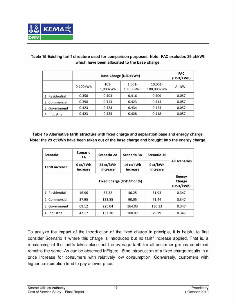
Kosrae Utilities Authority Proprietary Cost of Service Study – Final Report 1 October 2012
46
Table 15 Existing tariff structure used for comparison purposes. Note: FAC excludes 29 ct/kWh
which have been allocated to the base charge.
Base Charge (USD/kWh) FAC
(USD/kWh)
0-100kWh 101-
1,000kWh
1,001-
10,000kWh
10,001-
100,000kWh All kWh
1. Residential 0.358 0.403 0.416 0.409 0.057
2. Commercial 0.398 0.413 0.423 0.414 0.057
3. Government 0.423 0.423 0.434 0.424 0.057
4. Industrial 0.423 0.423 0.428 0.418 0.057
Table 16 Alternative tariff structure with fixed charge and separation base and energy charge.
Note: the 29 ct/kWh have been taken out of the base charge and brought into the energy charge.
Scenario: Scenario
1A Scenario 2A Scenario 3A Scenario 3B
All scenarios
Tariff increase: 0 ct/kWh
increase
23 ct/kWh
increase
14 ct/kWh
increase
9 ct/kWh
increase
Fixed Charge (USD/month)
Energy
Charge
(USD/kWh)
1. Residential 16.96 55.22 40.25 31.93 0.347
2. Commercial 37.95 123.55 90.05 71.44 0.347
3. Government 69.12 225.04 164.03 130.13 0.347
4. Industrial 42.17 137.30 100.07 79.39 0.347
To analyze the impact of the introduction of the fixed charge in principle, it is helpful to first
consider Scenario 1 where this charge is introduced but no tariff increase applied. That is, a
rebalancing of the tariffs takes place but the average tariff for all customer groups combined
remains the same. As can be observed inFigure 18the introduction of a fixed charge results in a
price increase for consumers with relatively low consumption. Conversely, customers with
higher consumption tend to pay a lower price.
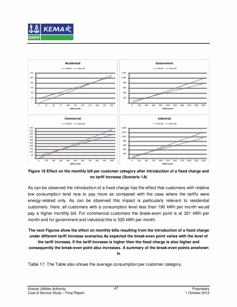
Kosrae Utilities Authority Proprietary Cost of Service Study – Final Report 1 October 2012
47
Figure 18 Effect on the monthly bill per customer category after introduction of a fixed charge and
no tariff increase (Scenario 1A)
As can be observed the introduction of a fixed charge has the effect that customers with relative
low consumption tend now to pay more as compared with the case where the tariffs were
energy-related only. As can be observed this impact is particularly relevant to residential
customers. Here, all customers with a consumption level less than 190 kWh per month would
pay a higher monthly bill. For commercial customers the break-even point is at 321 kWh per
month and for government and industrial this is 520 kWh per month.
The next Figures show the effect on monthly bills resulting from the introduction of a fixed charge
under different tariff increase scenarios.As expected the break-even point varies with the level of
the tariff increase. If the tariff increase is higher then the fixed charge is also higher and
consequently the break-even point also increases. A summary of the break-even points areshown
in
Table 17. The Table also shows the average consumption per customer category.
-
20
40
60
80
100
120
0 25 50 75 100 125 150 175 200 225 250
kWh/month
Residential
Old Bill New Bill
-
50
100
150
200
250
300
350
400
450
500
0 100 200 300 400 500 600 700 800 900 1000
kWh/month
Commercial
Old Bill New Bill
-
200
400
600
800
1,000
1,200
0 200 400 600 800 1000 1200 1400 1600 1800 2000
kWh/month
Government
Old Bill New Bill
-
200
400
600
800
1,000
1,200
1,400
0 250 500 750 1000 1250 1500 1750 2000 2250 2500
kWh/month
Industrial
Old Bill New Bill
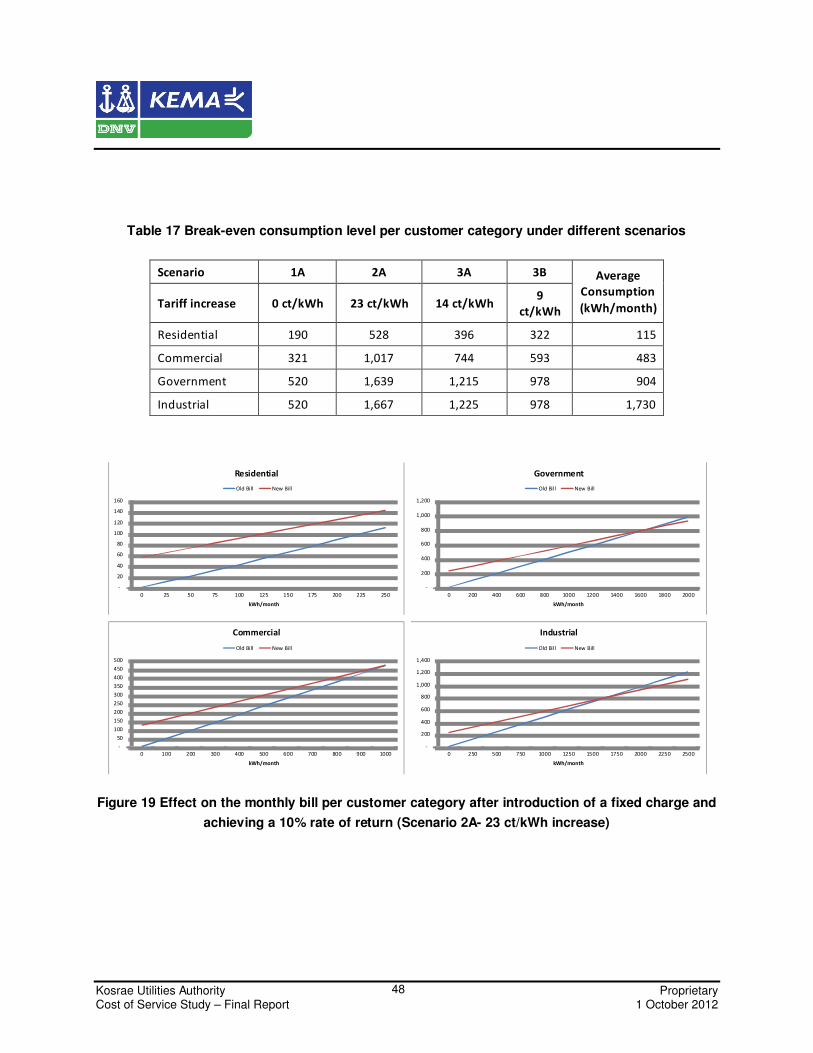
Kosrae Utilities Authority Proprietary Cost of Service Study – Final Report 1 October 2012
48
Table 17 Break-even consumption level per customer category under different scenarios
Scenario 1A 2A 3A 3B Average
Consumption
(kWh/month) Tariff increase 0 ct/kWh 23 ct/kWh 14 ct/kWh 9
ct/kWh
Residential 190 528 396 322 115
Commercial 321 1,017 744 593 483
Government 520 1,639 1,215 978 904
Industrial 520 1,667 1,225 978 1,730
Figure 19 Effect on the monthly bill per customer category after introduction of a fixed charge and
achieving a 10% rate of return (Scenario 2A- 23 ct/kWh increase)
-
20
40
60
80
100
120
140
160
0 25 50 75 100 125 150 175 200 225 250
kWh/month
Residential
Old Bi ll New Bill
-
50
100
150
200
250
300
350
400
450
500
0 100 200 300 400 500 600 700 800 900 1000
kWh/month
Commercial
Old Bi ll New Bill
-
200
400
600
800
1,000
1,200
0 200 400 600 800 1000 1200 1400 1600 1800 2000
kWh/month
Government
Old Bil l New Bill
-
200
400
600
800
1,000
1,200
1,400
0 250 500 750 1000 1250 1500 1750 2000 2250 2500
kWh/month
Industrial
Old Bil l New Bill
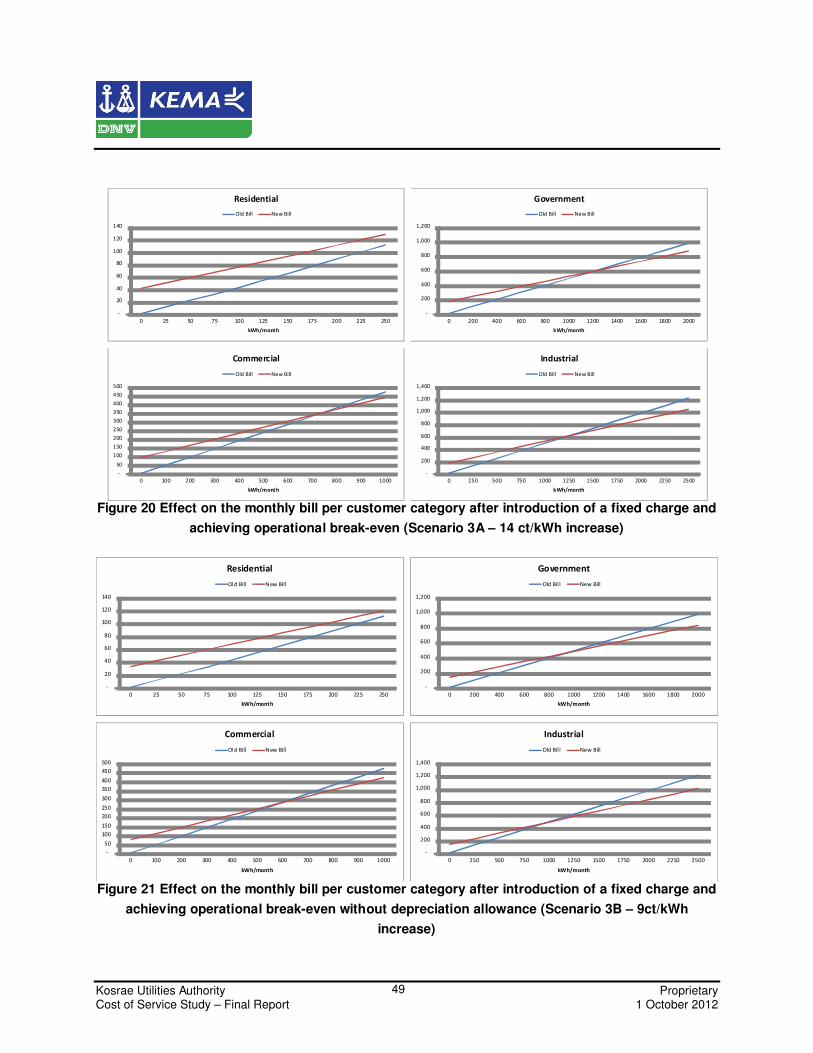
Kosrae Utilities Authority Proprietary Cost of Service Study – Final Report 1 October 2012
49
Figure 20 Effect on the monthly bill per customer category after introduction of a fixed charge and
achieving operational break-even (Scenario 3A – 14 ct/kWh increase)
Figure 21 Effect on the monthly bill per customer category after introduction of a fixed charge and
achieving operational break-even without depreciation allowance (Scenario 3B – 9ct/kWh
increase)
-
20
40
60
80
100
120
140
0 25 50 75 100 125 150 175 200 225 250
kWh/month
Residential
Old Bill New Bill
-
50
100
150
200
250
300
350
400
450
500
0 100 200 300 400 500 600 700 800 900 1000
kWh/month
Commercial
Old Bill New Bill
-
200
400
600
800
1,000
1,200
0 200 400 600 800 1000 1200 1400 1600 1800 2000
kWh/month
Government
Old Bill New Bill
-
200
400
600
800
1,000
1,200
1,400
0 250 500 750 1000 1250 1500 1750 2000 2250 2500
kWh/month
Industrial
Old Bill New Bill
-
20
40
60
80
100
120
140
0 25 50 75 100 125 150 175 200 225 250
kWh/month
Residential
Old Bill New Bill
-
50
100
150
200
250
300
350
400
450
500
0 100 200 300 400 500 600 700 800 900 1000
kWh/month
Commercial
Old Bill New Bill
-
200
400
600
800
1,000
1,200
0 200 400 600 800 1000 1200 1400 1600 1800 2000
kWh/month
Government
Old Bil l New Bill
-
200
400
600
800
1,000
1,200
1,400
0 250 500 750 1000 1250 1500 1750 2000 2250 2500
kWh/month
Industrial
Old Bil l New Bill

Kosrae Utilities Authority Proprietary Cost of Service Study – Final Report 1 October 2012
50
5 Conclusions and Recommendations
5.1 Conclusions
The purpose of this project was to perform a review of KUA’s tariffs and develop
recommendations on an appropriate tariff structure and on mechanisms to adjust the tariffs.
This task was approached from two main perspectives (1) the tariff level, and (2) the tariff
structure. The following conclusions can be drawn based on the analysis performed.
5.1.1 Tariff Level Analysis
KUA’s financial performance has been evaluated. For this purpose a financial model was
developed as described in Section 2. This model was applied in Section 3 to evaluate the
existing tariffs and to compute the necessary tariff adjustment under different scenarios.
Analysis showed that existing tariffs in use by KUA are below costs and if not increased will
result in (further) serious financial impact for KUA. After this it was computed what kind of tariff
increase would be necessary to bring financial performance to an adequate level. Here,
“adequate” can be interpreted in different ways, each resulting in a different necessary tariff
increase:
• If KUA were to be financially sound with a rate of return of 10% implying the company
having full ability to independently undertake all investment, then the necessary tariff
increase would be 23 ct/kWh.
• If KUA were to remain dependent on external grants for financing investment the criteria
would be assurance of a balance between operational income and expenses. In that
case the necessary tariff increase would be 14 ct/kWh (with ability to independently
renew these investments in future) or 9 ct/kWh (with future renewals also being
dependent on grants).
Kosrae Utilities Authority Proprietary Cost of Service Study – Final Report 1 October 2012
51
5.1.2 Tariff StructureAnalysis
In Section 4 the analysis of the existing tariff structure was undertaken. This analysis helped to
assess the degree of alignment between the true costs and the tariff paid per type of customer.
From an economic point of view an alignment between these two is desired as cost
reflectiveness helps to promote efficiency.
The costs per customer category within the KUA customer base was computed in three steps
namely functionalization, classification, and allocation. Using this method the costs incurred by
KUA for each group was computed. This was compared to the actual tariff paid by customers.
Comparisons showed that there is a misalignmentfor all customer groups. Overall customers
pay a price that is lower than actual costs (which is in line with the conclusions from the tariff
level analysis). The mismatch is particularly visible for domestic customers.
The misalignment can be taken away by introducing a fixed charge, which better aligns the
costs and tariff per customer group. The disadvantage of this however is that rebalancing in the
monthly bill will take place. Customers with low consumption will then be paying a higher bill and
vice versa.
5.2 Recommendations
The main conclusion from the analysis is that an adjustment in KUA’s tariffs will be necessary.
The issue therefore is not whether or not such an adjustment should take place, but rather the
way in which this should come. This ultimately will be a policy decision by KUA. In order to
accommodate this process the following decision trees can be useful.
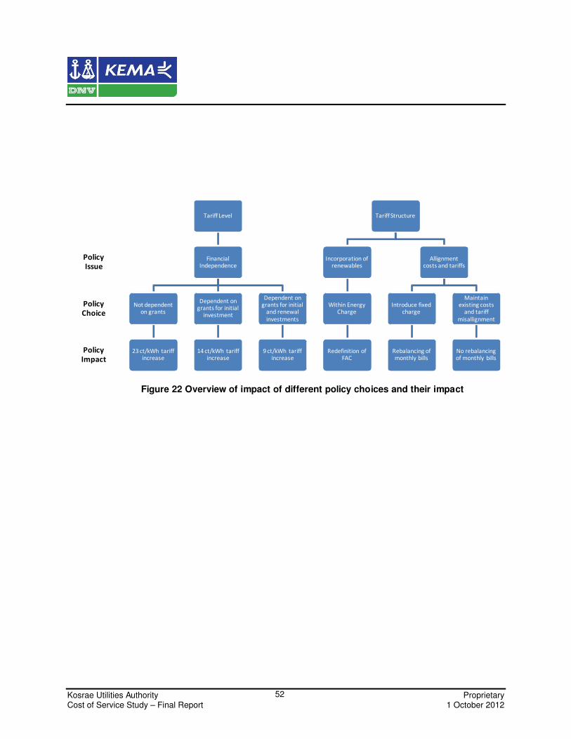
Kosrae Utilities Authority Proprietary Cost of Service Study – Final Report 1 October 2012
52
Figure 22 Overview of impact of different policy choices and their impact
Policy Issue
Policy Choice
Policy Impact
Tariff Level
Financial Independence
Not dependent on grants
23 ct/kWh tariff increase
Dependent on grants for initial
investment
14 ct/kWh tariff increase
Dependent on grants for initial
and renewal
investments
9 ct/kWh tariff increase
Tariff Structure
Incorporation of renewables
Within Energy Charge
Redefinition of FAC
Allignment costs and tariffs
Introduce fixed charge
Rebalancing of monthly bills
Maintain existing costs
and tariff
misallignment
No rebalancing of monthly bills
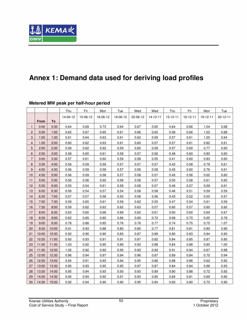
Kosrae Utilities Authority Proprietary Cost of Service Study – Final Report 1 October 2012
53
Annex 1: Demand data used for deriving load profiles
Metered MW peak per half-hour period
Thu Fri Mon Tue Wed Wed Thu Fri Mon Tue
From To
14-06-12 15-06-12 18-06-12 19-06-12 20-06-12 14-12-11 15-12-11 16-12-11 19-12-11 20-12-11
1 0:00 0:30 0.64 0.69 0.73 0.64 0.67 0.65 0.64 0.66 1.04 0.68
2 0:30 1:00 0.62 0.67 0.65 0.61 0.66 0.62 0.58 0.66 1.02 0.68
3 1:00 1:30 0.61 0.64 0.63 0.61 0.62 0.59 0.57 0.61 1.00 0.64
4 1:30 2:00 0.60 0.62 0.63 0.61 0.60 0.57 0.57 0.61 0.82 0.61
5 2:00 2:30 0.59 0.62 0.62 0.59 0.60 0.59 0.57 0.60 0.77 0.60
6 2:30 3:00 0.58 0.60 0.61 0.59 0.57 0.56 0.48 0.60 0.80 0.60
7 3:00 3:30 0.57 0.61 0.60 0.59 0.58 0.55 0.41 0.60 0.83 0.60
8 3:30 4:00 0.56 0.59 0.59 0.57 0.57 0.57 0.42 0.58 0.79 0.61
9 4:00 4:30 0.56 0.59 0.58 0.57 0.56 0.58 0.45 0.60 0.76 0.61
10 4:30 5:00 0.56 0.59 0.58 0.57 0.58 0.57 0.45 0.56 0.62 0.60
11 5:00 5:30 0.56 0.56 0.60 0.58 0.58 0.57 0.50 0.58 0.61 0.60
12 5:30 6:00 0.55 0.54 0.61 0.59 0.58 0.57 0.46 0.57 0.59 0.61
13 6:00 6:30 0.56 0.54 0.57 0.54 0.58 0.58 0.46 0.51 0.59 0.59
14 6:30 7:00 0.57 0.57 0.58 0.55 0.58 0.56 0.43 0.52 0.55 0.57
15 7:00 7:30 0.59 0.60 0.61 0.59 0.62 0.55 0.47 0.54 0.61 0.59
16 7:30 8:00 0.59 0.62 0.63 0.62 0.63 0.57 0.60 0.57 0.60 0.60
17 8:00 8:30 0.63 0.60 0.66 0.69 0.62 0.61 0.60 0.60 0.69 0.67
18 8:30 9:00 0.62 0.65 0.80 0.66 0.69 0.72 0.69 0.70 0.65 0.78
19 9:00 9:30 0.78 0.88 0.85 0.76 0.76 0.77 0.74 0.75 0.75 1.07
20 9:30 10:00 0.91 0.93 0.88 0.80 0.85 0.77 0.81 0.81 0.80 0.90
21 10:00 10:30 0.92 0.90 0.90 0.83 0.87 0.89 0.80 0.83 0.84 0.90
22 10:30 11:00 0.93 0.93 0.91 0.91 0.87 0.82 0.84 0.85 0.87 0.85
23 11:00 11:30 1.03 0.92 0.95 0.89 0.93 0.88 0.84 0.88 0.85 1.00
24 11:30 12:00 1.02 0.92 0.92 0.95 0.93 0.92 0.91 0.94 0.67 0.98
25 12:00 12:30 0.96 0.94 0.97 0.94 0.96 0.87 0.89 0.84 0.70 0.94
26 12:30 13:00 0.94 0.91 0.93 0.94 0.95 0.86 0.88 0.86 0.62 0.92
27 13:00 13:30 0.95 0.93 0.95 0.95 0.97 0.87 0.84 0.84 0.68 0.93
28 13:30 14:00 0.95 0.94 0.93 0.93 0.93 0.89 0.80 0.88 0.72 0.92
29 14:00 14:30 0.95 0.94 0.92 0.91 0.93 0.85 0.84 0.81 0.69 0.90
30 14:30 15:00 0.92 0.94 0.90 0.90 0.95 0.84 0.83 0.80 0.70 0.90
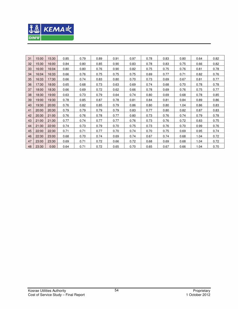
Kosrae Utilities Authority Proprietary Cost of Service Study – Final Report 1 October 2012
54
31 15:00 15:30 0.85 0.79 0.89 0.91 0.97 0.78 0.83 0.80 0.64 0.82
32 15:30 16:00 0.84 0.80 0.85 0.90 0.83 0.78 0.83 0.75 0.66 0.82
33 16:00 16:04 0.80 0.80 0.76 0.90 0.82 0.75 0.75 0.76 0.81 0.78
34 16:04 16:33 0.66 0.76 0.75 0.75 0.75 0.69 0.77 0.71 0.82 0.76
35 16:33 17:30 0.66 0.74 0.83 0.80 0.70 0.73 0.69 0.67 0.81 0.77
36 17:30 18:00 0.65 0.68 0.73 0.63 0.69 0.74 0.68 0.70 0.78 0.78
37 18:00 18:30 0.66 0.69 0.72 0.62 0.66 0.78 0.69 0.76 0.75 0.77
38 18:30 19:00 0.63 0.73 0.79 0.64 0.74 0.80 0.69 0.68 0.78 0.85
39 19:00 19:30 0.78 0.85 0.87 0.78 0.81 0.84 0.81 0.84 0.89 0.86
40 19:30 20:00 0.76 0.82 0.85 0.79 0.86 0.80 0.80 1.04 0.86 0.83
41 20:00 20:30 0.79 0.79 0.79 0.79 0.83 0.77 0.80 0.82 0.87 0.83
42 20:30 21:00 0.76 0.76 0.78 0.77 0.80 0.73 0.76 0.74 0.79 0.78
43 21:00 21:30 0.77 0.74 0.77 0.77 0.76 0.73 0.76 0.72 0.83 0.75
44 21:30 22:00 0.74 0.73 0.79 0.70 0.75 0.73 0.76 0.70 0.99 0.76
45 22:00 22:30 0.71 0.71 0.77 0.70 0.74 0.70 0.75 0.69 0.95 0.74
46 22:30 23:00 0.68 0.70 0.74 0.69 0.74 0.67 0.74 0.68 1.04 0.72
47 23:00 23:30 0.69 0.71 0.72 0.66 0.72 0.68 0.69 0.68 1.04 0.72
48 23:30 0:00 0.64 0.71 0.72 0.65 0.70 0.65 0.67 0.66 1.04 0.70
Kosrae Utilities Authority Proprietary Cost of Service Study – Final Report 1 October 2012
55
Annex 2: Cost of Capital
The standard methodology to determine the cost of capital of a business is the Weighted
Average Cost of Capital, WACC. The WACC is the average of the cost of debt and the cost of
equity, the two components of the capital structure of the company, weighted by their share on
total capital. It is, therefore, the weighted average return required by the lenders and
shareholders of the company, that is, by its providers of capital. The WACC is also used for
regulated businesses, since it allows the companies to earn the normal rate of return that is
expected in competitive markets.
In order to derive the WACC for a particular company, a significant amount of data is necessary.
For the specific case of KUA it should be noted that most of these data were not available, in
particular due to the absence of mature financial markets in Micronesia. Therefore a number of
assumptions had to be made in order to arrive at a reasonable estimation for the WACC.
WACC Formula
The general formulas used to calculate the WACC can be expressed as follows:
WACC = wd . kd + we . ke
wd= D/(D+E), we= E/(D+E)
Where:
• kd: cost of debt
• ke: cost of equity
• D: value of firm's debt
• E: value of firm's equity
This is the so-called nominal WACC since it is computed in nominal terms.Note that as
corporate taxes are not applicable to KUA no adjustments for this need to be made in the
WACC (i.e. the pre-tax and post-tax WACCs are the same).
Kosrae Utilities Authority Proprietary Cost of Service Study – Final Report 1 October 2012
56
For the purposes of this analysis, we will estimate KUA’s WACC in nominal terms and referred
to in USD dollars. The following sections describe the criteria and calculation of the different
components of the WACC.
Capital Structure and Cost of Debt
Most firms use both debt and equity to fund their business and the relationship between these
two sources of funds provides the firm’s capital structure ratios or gearing ratios or leverage
ratios. The analysis of a firm’s capital structure is essential to evaluate its long-term risk and
return prospects. Since debt carries fixed-interest and repayment commitments, a highly geared
firm (i.e. a firm with large fraction of debt in its invested capital) has greater chances of failing on
its financial commitments and being forced into bankruptcy. As such, highly leveraged firms are
more vulnerable to business downturns than those with lower debt to worth positions. Also, for
the same reason, the returns for equity shareholders (who are the residual claimants in the
company) become more volatile and risky as gearing increases. Finally, a high level of gearing
may also have implications for the extent to which a company may have access to additional
capital.
One indicator of the amount of leverage used by a business is the Gearing Ratio. This ratio
indicates the level of debt in proportion to total capital (debt + equity). A high gearing indicates
an extensive use of leverage i.e. a large proportion of financing provided by creditors. A low
gearing, on the other hand, indicates that the business is making little use of leverage.
Currently the level of long-term debt in KUA’s books is equal to zero. This implies a debt level of
0%, which would not be observed in normal circumstances. The present situation could be
explained by the fact that KUA currently is primarily dependent on grants for financing
investments. Furthermore it may seem that the current financial performance of the company
would make it more difficult to attract commercial loans.
At the same time the purpose of the WACC computation is to estimate KUA’s costs of capital
assuming a normal mode of business i.e. sufficiently high income to finance investments
through a considerable degree of own funding. Generally, a gearing of 2/3 is considered to be
appropriate. That is, 2/3 of the investment would be financed by external capital sources (loans)
Kosrae Utilities Authority Proprietary Cost of Service Study – Final Report 1 October 2012
57
and 1/3 through own funds (equity). For the purpose of WACC computation this number of 2/3
will therefore be assumed.
An evaluating of past interest payments and considering future expected developments the
average debt cost is estimated at 7.5%. Consequently a value of kd = 7.5% will be used as debt
cost for the present calculation.
Cost of Equity
There are several approaches to estimate the cost of equity. The most common method used in
the business and regulatory practice is based in the Capital Asset Pricing Model or CAPM. The
CAPM states that in efficient markets investors should be compensated for the systematic risk
they take, that is, the risk non diversifiable through portfolio diversification. In simple terms, the
risk-adjusted return is composed of a risk free rate of return and an equity risk premium. The
equity risk premium ERP can be higher or lower than the average market return, depending on
the correlation between the returns of the specific investment and the returns of the capital
market as a whole.
The general formula for the cost of equity according to the CAPM methodology is:
ke = Rf + β.[E(Rm) – Rf]
Where Rf: Risk-free rate of return
E(Rm): Expected rate of return of the market
β: beta, measure of systematic risk of the equity investment
E(Rm) – Rf: market risk premium
The Beta (β) parameter is a measure of the sensitivity of the business to the general economic
cycles, being positive when the business return moves in the same direction of the market and
negative if it moves in the opposite way. A Beta value equal to 1 indicates that the business
follows the cycles of the economic activity as reflected in the average market returns, and
should earn this same rate of return. Business with risk lower than the average have a Beta less
than 1 and require lower rates of return.
The calculations of ke depend on data availability and the specific conditions of the business.
For KUA, there is no market information available in the context of a national or regional
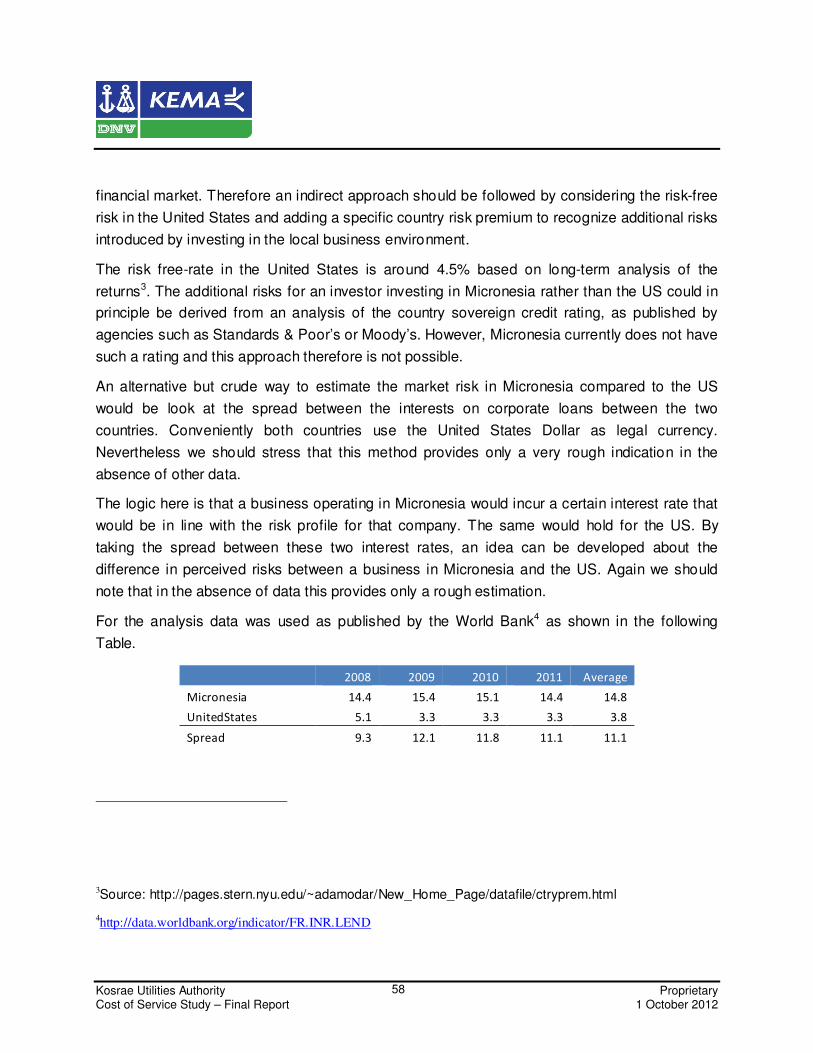
Kosrae Utilities Authority Proprietary Cost of Service Study – Final Report 1 October 2012
58
financial market. Therefore an indirect approach should be followed by considering the risk-free
risk in the United States and adding a specific country risk premium to recognize additional risks
introduced by investing in the local business environment.
The risk free-rate in the United States is around 4.5% based on long-term analysis of the
returns3. The additional risks for an investor investing in Micronesia rather than the US could in
principle be derived from an analysis of the country sovereign credit rating, as published by
agencies such as Standards & Poor’s or Moody’s. However, Micronesia currently does not have
such a rating and this approach therefore is not possible.
An alternative but crude way to estimate the market risk in Micronesia compared to the US
would be look at the spread between the interests on corporate loans between the two
countries. Conveniently both countries use the United States Dollar as legal currency.
Nevertheless we should stress that this method provides only a very rough indication in the
absence of other data.
The logic here is that a business operating in Micronesia would incur a certain interest rate that
would be in line with the risk profile for that company. The same would hold for the US. By
taking the spread between these two interest rates, an idea can be developed about the
difference in perceived risks between a business in Micronesia and the US. Again we should
note that in the absence of data this provides only a rough estimation.
For the analysis data was used as published by the World Bank4 as shown in the following
Table.
2008 2009 2010 2011 Average
Micronesia 14.4 15.4 15.1 14.4 14.8
UnitedStates 5.1 3.3 3.3 3.3 3.8
Spread 9.3 12.1 11.8 11.1 11.1
3Source: http://pages.stern.nyu.edu/~adamodar/New_Home_Page/datafile/ctryprem.html
4http://data.worldbank.org/indicator/FR.INR.LEND
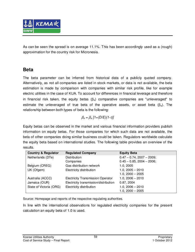
Kosrae Utilities Authority Proprietary Cost of Service Study – Final Report 1 October 2012
59
As can be seen the spread is on average 11.1%. This has been accordingly used as a (rough)
approximation for the country risk for Micronesia.
Beta
The beta parameter can be inferred from historical data of a publicly quoted company.
Alternatively, as not all companies are listed in stock markets, or data is not available, the beta
estimation is made by comparison with companies with similar risk profile, like for example
electric utilities in the case of KUA. To account for differences in financial leverage and therefore
in financial risk taken, the equity betas (βe) comparative companies are "unleveraged" to
estimate the unleveraged of true beta of the operative assets, or asset beta (βa). The
relationship between both types of beta is the following:
βe = βa [1+(D/E)(1-τ)]
Equity betas can be observed in the market and various financial information providers publish
information on equity betas. For those companies for which such data are not available, the
beta of other companies doing similar business could be taken. Regulators worldwide calculate
the equity beta based on international studies. The following table provides an overview of the
results.
Country & Regulator Regulated Company Equity Beta
Netherlands (DTe) Distribution
Companies
0.47 – 0.74, 2007 – 2009;
0.45 – 0.85, 2004 – 2006;
Belgium (CREG) Gas distribution network 1.0, 2005
UK (Ofgem) Electricity distribution 1.0, 2005 – 2010
1.0, 2000 – 2005
Australia (ACCC) Electricity Transmission Operator 1.0, 2006 – 2010
Jamaica (OUR) Electricity transmission/distribution 0.87, 2004
State of Victoria (ORG) Electricity distribution 1.0, 2006 – 2010
1.0, 2000 – 2005
Source: Homepage and reports of the respective regulating authorities.
In line with the international observations for regulated electricity companies for the present
calculation an equity beta of 1.0 is used.

Kosrae Utilities Authority Proprietary Cost of Service Study – Final Report 1 October 2012
60
WACC estimation
The application of the different parameters selected and the WACC calculations are
summarized in the following table. The estimated forward-looking WACC for KUA is estimated
at aound10%.
Parameter / Value Reference
Tax rate 0.0% Corporate tax rate
Debt Ratio, Wd 66.7% Assumed capital structure
Cost of Debt, kd 7.50% Company's financing cost
Post-tax Cost of Debt, Kd*(1-T) 7.50%
Equity Ratio, We 33.3% Assumed capital structure
Risk-free rate, Rf 4.5% US Government long-term bonds
Market risk premium, E(Rm) 11.2% Corporate interest spread
Equity Beta, Be 1.00 Leveraged beta
Cost of Equity, Ke 15.70% CAPM
WACC, post tax nominal 10.23%