Embed Size (px)
Citation preview
arX
iv:0
804.
1357
v2 [
hep-
th]
4 A
ug 2
008
Stationary ring solitons in field theory –
knots and vortons
Eugen Radu∗ and Mikhail S. Volkov†
Laboratoire de Mathematiques et Physique Theorique CNRS-UMR 6083,
Universite de Tours, Parc de Grandmont,
37200 Tours, FRANCE
We review the current status of the problem of constructing classical field theory
solutions describing stationary vortex rings in Minkowski space in 3 + 1 dimen-
sions. We describe the known up to date solutions of this type, such as the static
knot solitons stabilized by the topological Hopf charge, the attempts to gauge them,
the anomalous solitons stabilized by the Chern-Simons number, as well as the non-
Abelian monopole and sphaleron rings. Passing to the rotating solutions, we first
discuss the conditions insuring that they do not radiate, and then describe the spin-
ningQ-balls, their twisted and gauged generalizations reported here for the first time,
spinning skyrmions, and rotating monopole-antimonopole pairs. We then present the
first explicit construction of global vortons as solutions of the elliptic boundary value
problem, which demonstrates their non-radiating character. Finally, we describe the
analogs of vortons in the Bose-Einstein condensates, analogs of spinning Q-balls
in the non-linear optics, and also moving vortex rings in superfluid helium and in
ferromagnetics.
PACS numbers: 11.10.Lm, 11.27.+d, 98.80.Cq
to appear in Physics Reports
2
Contents
I. Introduction 3
II. Knot solitons 7
A. Faddeev-Skyrme model 7
B. Hopf charge 9
C. Topological bound and the N = 1, 2 hopfions 12
D. Unknots, links and knots 15
E. Conformally invariant knots 20
F. Can one gauge the knot solitons ? 21
G. Faddeev-Skyrme model versus semilocal Abelian Higgs model 22
H. Energy bound in the Abelian Higgs model 23
I. The issue of charge fixing 24
J. Searching for gauged knots 25
III. Knot solitons in gauge field theory 26
A. Anomalous solitons 26
B. Non-Abelian rings 29
1. Yang-Mills-Higgs theory 30
2. Monopole rings 30
3. Sphaleron rings 33
IV. Angular momentum and radiation in field systems 33
A. Angular momentum for stationary solitons 35
1. The case of manifest symmetries – no go results 36
2. The case of non-manifest symmetries 39
3. Spinning solitons as solutions of elliptic equations 40
V. Explicit examples of stationary spinning solitons 41
A. Q-balls 41
1. Non-spinning Q-balls 44
2. Spinning Q-balls 46
3. Twisted Q-balls 51

3
4. Spinning gauged Q-balls 52
5. Spinning interacting Q-balls 54
B. Skyrmions 55
1. Skyrme versus Faddeev-Skyrme 57
2. Spinning skyrmions 58
3. Spinning gauged skyrmions 60
C. Rotating monopole-antimonopole pairs 61
VI. Vortons 65
A. The Witten model 65
B. Vorton topology and boundary conditions 67
C. The sigma model limit 71
D. Explicit vorton solutions 72
VII. Ring solitons in non-relativistic systems 79
A. Vortons versus ‘skyrmions’ in Bose-Einstein condensates 80
B. Spinning rings in non-linear optics – Q-balls as light bullets 82
C. Moving vortex rings 84
1. Moving vortex rings in the superfluid helium 86
2. Moving magnetic rings 88
VIII. Concluding remarks 90
References 93
I. INTRODUCTION
Stationary vortex loops are often discussed in the literature in various contexts ranging
from the models of condensed matter physics [11], [12], [17], [41], [124], [137], [146], [147],
[149], to high energy physics and cosmology [29], [45], [46], [48], [165], [177]. Such objects
could be quite interesting physically and might be responsible for a plenty of important
physical phenomena, starting from the structure of quantum superfluids [54] and Bose-
Einstein condensed alkali gases [117] to the baryon asymmetry of the Universe, dark matter,
and the galaxy formation [165]. These intriguing physical aspects of vortex loops occupy

4
therefore most of the discussions in the literature, while much less attention is usually
payed to their mathematical existence. In most considerations the existence of such loops is
discussed only qualitatively, using plausibility arguments, and the problem of constructing
the corresponding field theory solutions is rarely addressed, such that almost no solutions
of this type are explicitly known.
The physical arguments usually invoked to justify the loop existence arise within the
effective macroscopic description of vortices [1], [129]. Viewed from large distances, their
internal structure can be neglected and the vortices can be effectively described as elastic
thin ropes or, if they carry currents, as thin wires [32], [33], [34], [35], [122]. This suggests
the following engineering procedure: to ‘cut out’ a finite piece of the vortex, then ‘twist’
it several times and finally ‘glue’ its ends. The resulting loop will be stabilized against
contraction by the potential energy of the twist deformation, that is by the positive pressure
contributed by the current and stresses [43], [42], [86], [130]. Equally, instead of twisting the
rope, one can first ‘make’ a loop and then ‘spin it up’ thus giving to it an angular momentum
to stabilize it against shrinking [47], [48]. Depending on whether they are spinning or not,
such loops are often called in the literature vortons and knots (also springs), respectively.
These macroscopic arguments are suggestive. However, they cannot guarantee the exis-
tence of loops as stationary field theory objects, since they do not take into account all the
field degrees of freedom that could be essential. Speaking more rigorously, one can prepare
twisted or spinning loop configurations as the initial data for the fields. However, nothing
guarantees that these data will evolve to non-trivial equilibrium field theory objects, since,
up to few exceptions, the typical field theory models under consideration do not have a
topological energy bound for static loop solitons. For spinning loops the situation can be
better, since the angular momentum can provide an additional stabilization of the system.
However, nothing excludes the possibility of radiative energy leakages from spinning loops.
Since there is typically a current circulating along them, which means an accelerated motion
of charges, it seems plausible that spinning loops should radiate, in which case they would
not be stationary but at best only quasistationary. In fact, loop formation is generically
observed in dynamical vortex network simulations (although for currentless vortices), and
these loops indeed radiate rapidly away all their energy (see e.g. [26]).
The lack of explicit solutions renders the situation even more controversial. In fact,
although there are explicit examples of loop solitons in global field theory, which means
5
containing only scalar fields with global internal symmetries, almost nothing is known about
such solutions in gauge field theory. Vortons, for example, were initially proposed more than
20 years ago in the context of the local U(1)×U(1) theory of superconducting cosmic strings
of Witten [177]. However, not a single field theory solution of this type has been obtained
up to now. Search for static knot solitons in the Ginzburg-Landau type gauge field theory
models has already 30 years of history, the result being always negative. All this casts some
doubts on the existence of stationary, non-radiating vortex loops in physically interesting
gauge field theory models. However, rigorous no-go arguments are not known either. As a
result, there are no solid arguments neither for nor against the existence of such solutions.
Interestingly, exact solutions describing ring-type objects are known in curved space.
These are black rings in the multidimensional generalizations of General Relativity – spinning
toroidal black holes (see [58] for a review). It seems therefore that Einstein’s field equations,
notoriously known for their complexity, are easier to solve than the non-linear equations
describing loops made of interacting gauge and scalar fields in Minkowski space.
It should be emphasized that the problem here is not related to the dynamical stability
of these loops. In order to be stable or unstable they should first of all exist as stationary
field theory solutions. The problem is related to the very existence of such solutions. One
should be able to decide whether they exist or not, which is a matter of principle, and
this is the main issue that we address in this paper. Therefore, when talking about loops
stabilized by some forces, we shall mean the force balance that makes possible their existence,
and not the stability of these loops with respect to all dynamical perturbations. If they
exist, their dynamical stability should be analyzed separately, but we shall call solitons all
localized, globally regular, finite energy field theory solutions, irrespectively of their stability
properties. It should also be stressed that we insist on the stationarity condition for the
solitons, which implies the absence of radiation. Quasistationary loops which radiate slowly
and live long enough could also be physically interesting, but we are only interested in loops
which could live infinitely longtime, at least in classical theory.
Trying to clarify the situation, we review in what follows the known field theory solu-
tions in Minkowski space in 3 + 1 dimensions describing stationary ring objects. We shall
divide them in two groups, depending on whether they do have or do not have an angular
momentum. Solutions without angular momentum are typically static, that is they do not
depend on time and also do not typically have an electric field. We start by describing
6
the static knot solitons stabilized by the Hopf charge in a global field theory model. Then
we review the attempts to generalize these solutions within gauge field theory, with the
conclusion that some additional constraints on the gauge field are necessary, since fixing
only the Hopf charge does not seem to be sufficient to stabilize the system in this case. We
then consider two known examples of static ring solitons in gauge field theory: the anoma-
lous solitons stabilized by the Chern-Simons number, and the non-Abelian monopole and
sphaleron rings.
Passing to the rotating solutions, we first of all discuss the issue of how the presence of
an angular momentum, associated to some internal motions in the system, can be reconciled
with the absence of radiation which is normally generated by these motions. One possibility
for this is to consider time-independent solitons in theories with local internal symmetries.
They will not radiate, but it can be shown for a number of important field theory models
that the angular momentum vanishes in this case. Another possibility arises in systems with
global symmetries, where one can consider non-manifestly stationary and axisymmetric fields
containing spinning phases. Such fields could have a non-zero angular momentum, but the
absence of radiation is not automatically guaranteed in this case. The general conclusion
is that the existence of non-radiating spinning solitons, although not impossible, seems to
be rather restricted. Such solutions seem to exist only in some quite special field theory
models, while generic spinning field systems should radiate.
Nevertheless, non-radiating spinning solitons in Minkowski space in 3+1 dimensions exist,
and we review below all known examples: these are the spinning Q-balls, their twisted and
gauged generalizations, spinning Skyrmions and rotating monopole-antimonopole pairs. In
addition, there are also vortons, and below we present for the first time numerical solutions
of elliptic equations describing vortons in the global field theory limit. Although global
vortons have been studied before by different methods, our construction shows that they
indeed exist as stationary, non-radiating field theory objects.
We also discuss stationary ring solitons in non-relativistic physics. Surprisingly, it turns
out that the relativistic vortons can be mapped to the ‘skyrmion’ solutions of the Gross-
Pitaevskii equation in the theory of Bose-Einstein condensation. In addition, it turns out
that Q-balls can describe light pulses in media with non-linear refraction – ‘light bullets’.
Finally, for the sake of completeness, we discuss also the moving vortex rings stabilized by
the Magnus force in continuous media theories, such as in the superfluid helium and in

7
ferromagnetics.
In our numerical calculations we use an elliptic PDE solver with which we have managed
to reproduce most of the solutions we describe, as well as obtain a number of new results
presented below for the first time. The latter include the explicit vorton solutions, spinning
twisted Q-balls, spinning gauged Q-balls, as well as the ‘Saturn’, ‘hoop’ and bi-ring solutions
for the interacting Q-balls. We put the main emphasise on describing how the solutions are
constructed and not to their physical applications, so that our approach is just the opposite
and therefore complementary to the one generally adopted in the existing literature. As
a result, we outline the current status of the ring soliton existence problem – within the
numerical approach. Giving mathematically rigorous existence proofs is an issue that should
be analyzed separately. It seems that our global vorton solutions could be generalized in
the context of gauge field theory. The natural problem to attack would then be to obtain
vortons in the electroweak sector of Standard Model.
In this text the signature of the Minkowski spacetime metric gµν is chosen to be
(+,−,−,−), the spacetime coordinates are denoted by xµ = (x0, xk) ≡ (t,x) with k = 1, 2, 3.
All physical quantities discussed below, including fields, coordinates, coupling constants and
conserved quantities are dimensionless.
II. KNOT SOLITONS
Let us first consider solutions with zero angular momentum stabilized by their intrinsic
deformations. We shall start by discussing the famous example of static knotted solitons in
a non-linear sigma model. Since this is the best known and also in some sense canonical
example of knot solitons, we shall describe it in some detail. We shall then review the status
of gauge field theory generalizations of these solutions.
A. Faddeev-Skyrme model
More than 30 years ago Faddeev introduced a field theory consisting of a non-linear O(3)
sigma model augmented by adding a Skyrme-type term [61], [62]. This theory can also be
obtained by a consistent truncation of the O(4) Skyrme model (see Sec.VB1 below). Its

8
dynamical variables are three scalar fields n ≡ na = (n1, n2, n3) constraint by the condition
n · n =3∑
a=1
nana = 1,
so that they span a two-sphere S2. The Lagrangian density of the theory is
L[n] =1
32π2(∂µn · ∂µn− FµνFµν) (2.1)
where
Fµν =1
2ǫabcn
a∂µnb∂νn
c ≡ 1
2n · (∂µn× ∂νn). (2.2)
The Lagrangian field equations read
∂µ∂µn + ∂µFµν(n× ∂νn) = (n · ∂µ∂µn)n . (2.3)
In the static limit the energy of the system is
E[n] =1
32π2
∫
R3
(
(∂kn)2 + (Fik)2
)
d3x ≡ E2 + E4. (2.4)
Under scale transformations, x→ Λx, one has E2 → ΛE2 and E4 → E4/Λ. The energy will
therefore be stationary for Λ = 1 if only the virial relation holds,
E2 = E4. (2.5)
This shows that the four derivative term E4 is necessary, since otherwise the virial relation
would require that E2 = 0, thus ruling out all non-trivial static solutions – in agreement
with the Hobart-Derrick theorem [92], [52].
Any static field n(x) defines a map R3 → S2. Since for finite energy configurations n
should approach a constant value for |x| → ∞, all points at infinity of R3 map to one point
on S2. Using the global O(3)-symmetry of the theory one can choose this point to be the
north pole of the S2,
lim|x|→∞
n(x) = n∞ = (0, 0, 1). (2.6)
Notice that this condition leaves a residual O(2) symmetry of global rotations around the
third axis in the internal space,
n1 + in2 → (n1 + in2)eiα, n3 → n3. (2.7)
The position of the field configuration described by n(x) can now be defined as the set of
points where the field is as far as possible from the vacuum value, that is the preimage of the

9
point −n∞ antipodal to the vacuum +n∞. This preimage forms a closed loop (or collection
of loops) called position curve. Solitons in the theory can therefore be viewed as string-like
objects, stabilized by their topological charge to be defined below.
At the intuitive level, these solitons can be viewed as closed loops made of twisted vortices.
Specifically, the theory admits solutions describing straight vortices that can be parametrized
in cylindrical coordinates ρ, z, ϕ as n3 = cos Θ(ρ), n1+in2 = sin Θ(ρ) eipz+inϕ, where n ∈ Z
is the vortex winding number [111]. The phase pz+nϕ thus changes both along and around
the vortex and the vector n rotates around the third internal direction as one moves along
the vortex, which can be interpreted as twisting of the vortex. It seems plausible that a loop
made of a piece of length L of such a twisted vortex, where pL = 2πm, could be stabilized
by the potential energy of the twist deformation. For such a twisted loop the phase increases
by 2πn after a revolution around the vortex core and by 2πm as one travels along the loop,
where m ∈ Z is the number of twists. If the loop is homeomorphic to a circle, then the
product nm gives the value of its topological invariant: the Hopf charge.
B. Hopf charge
The condition (2.6) allows one to view the infinity of R3 as one point, thus effectively
replacing R3 by its one-point compactification S3. Any smooth field configuration can
therefore be viewed as a map
n(x) : S3 → S2. (2.8)
Any such map can be characterized by the topological charge N [n] ∈ π3(S2) = Z known as
the Hopf invariant. This invariant has a simple interpretation. The preimage of a generic
point on the target S2 is a closed loop. If a field has Hopf number N then the two loops
consisting of preimages of two generic distinct points on S2 will be linked exactly N times
(see Fig.1).
Although there is no local formula for N [n] in terms of n, one can give a non-local
expression as follows. The 2-form F = 12Fikdxi ∧ dxk defined by Eq.(2.2) is closed, dF = 0,
and since the second cohomology group of S3 is trivial, H(S3) = 0, there globally exists a
vector potential A = Akdxk such that F = dA. The Hopf index can then be expressed as
N [n] =1
8π2
∫
ǫijkAiFjk d3x. (2.9)

10
S2
(x)
n
n
1
2
n ) −1
(
FIG. 1: Preimages of any two points n1 and n2 on the target space S2 are two loops. The number
of mutual linking of these two loops is the Hopf charge N [n] of the map n(x). Here the case of
N = 1 is schematically shown.
For any smooth, finite energy field configuration n(x) this integral is integer-valued [119].
It can be shown that the maximal symmetry of n(x) compatible with a non-vanishing
Hopf charge is O(2) [111]. It follows that spherically symmetric fields are topologically
trivial. However, axially symmetric fields can have any value of the Hopf charge. Using
cylindrical coordinates such fields can be parametrized as [111]
n1 + in2 = ei(mϕ−nψ) sin Θ, n3 = cos Θ (2.10)
where n,m ∈ Z and Θ, ψ are functions of ρ, z. Since n → n∞ asymptotically, Θ should
vanish for r =√
ρ2 + z2 → ∞. The regularity at the z-axis requires for m 6= 0 that Θ
should vanish also there. As a result, one has n = n∞ both at the z-axis and at infinity,
that is at the contour C shown in Fig.2. Next, one assumes that n = −n∞ on a circle
S around the z-axis which is linked to C as shown in Fig.2 (more generally, one can have
n = −n∞ on several circles around the z-axis). The phase function ψ is supposed to increase
by 2π after one revolution along C. Since cos Θ interpolates between −1 and 1 on every
trajectory from S to C, it follows that surfaces of constant Θ are homeomorphic to tori.
The preimage of the point −n∞ consists of m copies of the circle S. The preimage of n∞
consists of n copies of the contour C. These two preimages are therefore linked mn times.
One can also compute F = dA according to (2.2), from where one finds
A = n cos2 Θ
2dψ +m sin2 Θ
2dϕ (2.11)
so that A∧F = nm cos2 Θ2
sin Θ dψ ∧ dΘ∧ dϕ. Inserting this to (2.9) gives the Hopf charge
N [n] = mn. (2.12)
Following Ref.[158], we shall call the fields given by the ansatz (2.10) Amn.

11
x
z
y
R
C
S
FIG. 2: Knot topology: the complex phase of the field in Eq.(2.10) winds along two orthogonal
directions: along S and along the contour C consisting of the z-axis and a semi-circle whose radius
expands to infinity. A similar winding of phases is found for other systems to be discussed below:
for vortons, skyrmions, and twisted Q-balls.
Let us consider two explicit examples of the Amn field. Let us introduce toroidal coordi-
nates u, v, ϕ such that
ρ = (R/τ) sinh u, z = (R/τ) sin v, (2.13)
where τ = cosh u − cos v with u ∈ [0,∞), v = [0, 2π). The correct boundary conditions for
the field will then be achieved by choosing in the ansatz (2.10)
Θ = Θ(u), ψ = v, (2.14)
where Θ(0) = 0, Θ(∞) = π.
Another useful parametrization is achieved by expressing na in terms of its complex
stereographic projection coordinate
W =n1 + in2
1 + n3. (2.15)
The values W = 0,∞ correspond to the vacuum and to the position curve of the soliton,
respectively. Passing to spherical coordinates r, ϑ, ϕ one introduces
φ = cosχ(r) + i sinχ(r) cosϑ, σ = sinχ(r) sinϑeiϕ, (2.16)

12
such that |φ|2 + |χ|2 = 1, where χ(0) = π, χ(∞) = 0. A particular case of the field (2.10) is
then obtained by setting
W =(σ)m
(φ)n. (2.17)
C. Topological bound and the N = 1, 2 hopfions
The following inequality for the energy (2.4) and Hopf charge (2.9) has been established
by Vakulenko and Kapitanski [163],
E[n] ≥ c|N [n]|3/4, (2.18)
where c = (3/16)3/8 [111]. Its derivation is non-trivial and proceeds via considering a
sequence of Sobolev inequalities. It is worth noting that a fractional power of the topological
charge occurs in this topological bound, whose value is optimal [119]. On the other hand,
it seems that the value of c can be improved, that is increased. Ward conjectures [171] that
the bound holds for c = 1, which has not been proven but is compatible with all the data
available. The existence of this bound shows that smooth fields attaining it, if exist, describe
topologically stable solitons. Constructing them implies minimizing the energy (2.4) with
fixed Hopf charge (2.9). Such minimum energy configurations are sometimes called in the
literature Hopf solitons or hopfions, and we shall call them fundamental or ground state
hopfions if they have the least possible energy for a given N .
Hopfions have been constructed for the first time for the lowest two values of the Hopf
charge, N = 1, 2 by Gladikowski and Hellmund [79] and almost simultaneously (although
somewhat more qualitatively) by Faddeev and Niemi [64]. Gladikowski and Hellmund used
the axial ansatz (2.10) expressed in toroidal coordinates, with Θ = Θ(u, v) and ψ = v +
ψ0(u, v), where Θ(0, v) = 0, Θ(∞, v) = π. Assuming the functions Θ(u, v) and ψ0(u, v) to be
periodic in v, they discretized the variables u, v and numerically minimized the discretized
expression for the energy with respect to the lattice cite values of Θ, ψ0. They found a
smooth minimum energy configuration of the A11 type for N = 1, while for N = 2 they
obtained two solutions, A21 and A12, the latter being more energetic than the former.
We have verified the results of Gladikowski and Hellmund by integrating the field equa-
tions (2.3) in the static, axially symmetric sector. Using the axial ansatz (2.10), the az-
imuthal variable ϕ decouples, and the equations reduce to two coupled PDE’s for Θ(ρ, z),
13
ψ(ρ, z). Unfortunately, these equations are rather complicated and it is not possible to re-
duce them to ODE’s by further separating variables, via passing to toroidal coordinates, say.
In fact, we are unaware of any attempts to solve these differential equations. We applied
therefore our numerical method described below in Sec.VI to integrate them, and we have
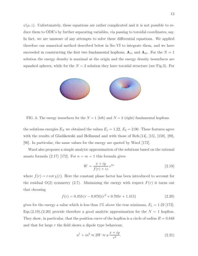
succeeded in constructing the first two fundamental hopfions, A11 and A21. For the N = 1
solution the energy density is maximal at the origin and the energy density isosurfaces are
squashed spheres, while for the N = 2 solution they have toroidal structure (see Fig.3). For
FIG. 3: The energy isosurfaces for the N = 1 (left) and N = 2 (right) fundamental hopfions.
the solutions energies EN we obtained the values E1 = 1.22, E2 = 2.00. These features agree
with the results of Gladikowski and Hellmund and with those of Refs.[14], [15], [158], [89],
[90]. In particular, the same values for the energy are quoted by Ward [172].
Ward also proposes a simple analytic approximation of the solutions based on the rational
ansatz formula (2.17) [172]. For n = m = 1 this formula gives
W =x+ iy
f(r) + izeiα (2.19)
where f(r) = r cotχ(r). Here the constant phase factor has been introduced to account for
the residual O(2) symmetry (2.7). Minimizing the energy with respect F (r) it turns out
that choosing
f(r) = 0.453 (r− 0.878)(r2 + 0.705r + 1.415) (2.20)
gives for the energy a value which is less than 1% above the true minimum, E1 = 1.22 [172].
Eqs.(2.19),(2.20) provide therefore a good analytic approximation for the N = 1 hopfion.
They show, in particular, that the position curve of the hopfion is a circle of radius R = 0.848
and that for large r the field shows a dipole type behaviour,
n1 + in2 ≈ 2W ≈ ax+ iy
r3. (2.21)

14
Ward also suggests the moduli space approximation in which the |N | = 1 hopfion is viewed as
an oriented circle (see Fig.4). There are six continuous moduli parameters: three coordinates
of the circle center, two angles determining the position of the circle axis, and also the overall
phase. Choosing arbitrarily a direction along the axis (shown by the vertical arrow in Fig.4),
there are two possible orientations corresponding to the sign of the Hopf charge, changing
which is achieved by W → W ∗. Although for one hopfion the phase is not important, the
relative phases of several hopfions determine their interactions.
Ward conjectures that well-separated hopfions interact as dipoles with the maximal at-
traction/repulsion when they are parallel/antiparallel, respectively, since the like charges
attract in a scalar field theory. He verifies this conjecture numerically, and then numerically
relaxes a field configuration corresponding to two mutually attracting hopfions. He discovers
two possible outcomes of this process. If the two hopfions are initially located in one plane
then they approach each other till the two circles merge to one thereby forming the A2,1
hopfion with N = 2. If they are initially oriented along the same line then they approach
each other but do not merge even in the energy minimum, where they remain separated by
a finite distance. This corresponds to the A1,2 hopfion, which is more energetic but locally
stable.
The A2,1 hopfion can be approximated by
W =(x+ iy)2eiα
f + i1.55 z r, f = 0.23(r − 1.27)(r + 0.44)(r + 0.16)(r2 − 2.15r + 5.09) (2.22)
whose energy is 1.5% above the true minimum, and there is also a similar approximation
for the A1,2 hopfion [172].
N=2N=−1N=1
2,1A A AA1,2−1,11,1
FIG. 4: Schematic representation of the hopfions as oriented circles

15
D. Unknots, links and knots
Similarly to the N = 1, 2 solutions, hopfions can be constructed within the axial ansatz
(2.10) also for higher values of n,m. However, for N > 2 they will not generically correspond
to the global energy minima. This can be understood if we remember that the Hopf charge
measures the amount of the twist deformation. Twisting an elastic rod shows that if it is
twisted too much then the loop made of it will not be planar, since it will find it energetically
favorable to bend toward the third direction. It is therefore expected that the ground state
hopfions for higher values of N will not be axially symmetric planar loops, but 3D loops,
generically without any symmetries.
The interest towards this issue was largely stirred by the work of Faddeev and Niemi [64],
[65], who conjectured that higher N hopfions should be not just closed lines but knotted
closed lines, with the degree of knotedness expressed in terms of the Hopf charge. In other
words, they conjectured that there could be a field theory realization of stable knots – the
idea that had been put forward by Lord Kelvin in the 19-th century [162] but never found
an actual realization. This knot conjecture of Faddeev and Niemi had a large resonance and
several groups had started large scale numerical simulations to look for knotted hopfions.
Such solutions have indeed been found, although not with quite the same properties as had
been originally predicted in Ref.[64], [65].
The first, really astonishing set of results has been reported by Battye and Sutcliffe [14],
[15], who managed to construct hopfions up to N = 8 and found the first non-trivial knot –
the trefoil knot – for N = 7. Similar analyses have been then independently carried out by
Hietarinta and Salo [89], [90] and also by Ward [171], [172], [176]. All groups performed the
full 3D energy minimization starting from an initial field configuration with a given N . Var-
ious initial configurations were used, as for example the ones given by the rational ansatz
(2.17), supplemented by non-axially symmetric perturbations to break the exact toroidal
symmetry. The value of N being constant during the relaxation, the numerical iterations
were found to converge to non-trivial energy minima, whose structure was sometimes com-
pletely different from that of the initial configuration (an online animation of the relaxation
process is available in [59]). Several local energy minima typically exist for a given N , some-
times with almost the same energy, so that it was not always easy to know whether the
minima obtained were local or global. Different initial configurations were therefore tried

16
to see if the minimum energy configurations could be reproduced in a different way. As a
result, it appears that the global energy minima have now been identified and cross-checked
up to N = 7 [90], [158], after which the analysis has been extended up to N = 16 [158]. The
properties of the solutions can be summarized as follows.
For N = 1, 2 these are the toroidal hopfions of Gladikowski and Hellmund [79], A11
and A21. Although initially obtained within the constrained, axially symmetric relaxation
scheme, they also correspond to the global minima of the full 3D energy functional. Axially
symmetric hopfions Am1 exist also for higher N = m [14], [15], but they no longer correspond
to global energy minima. For N = 3 the ground state hopfion is not planar and is called in
[158] A31, which can be viewed as deformed A31, with a pretzel-like position curve bent in
3D to brake the axial symmetry. However, for N = 4 the axial symmetry is restored again
in the ground state, A22, which seems to have a similar to the A12 two-ring structure [90],
[176]. The bent A41 also exists, but its energy it higher.
Up to now all hopfions have been the simplest knots topologically equivalent to a circle,
called unknots in the knot classification. A new phenomenon arises for N = 5, since the
fundamental hopfion in this case consists of two linked unknots. This has nothing to do
with the linking of preimages determining the value of N . This time the position curve itself
consists of two disjoint loops, corresponding to a charge 2 unknot linked to a charge 1 unknot.
The Hopf charge is not simply the sum of charges of each component, but contains in addition
the sum of their linking numbers due to their linking with the other components. It is worth
noting that the linking number of the oriented circles can be positive or negative, depending
on how they are linked [89] (see Fig.5). Using the notation of Ref.[158], the N = 5 hopfion
FIG. 5: Two possible ways to link N = 1 hopfions. Left: the total linking number is 2 = 1 + 1 and
the total charge if N = 1 + 1 + 2 = 4. Right: the total linking number is −2 = −1 − 1 and the
total charge is N = 1 + 1− 2 = 0. The numerical relaxation of these configurations gives therefore
completely different results [59].
can be called L1,11,2, where the subscripts label the Hopf charges of the unknot components of

17
the link, and the superscript above each subscript counts the extra linking number of that
component. The total Hopf charge is the sum of the subscripts plus superscripts. Similarly,
for N = 6 the ground state hopfion is a link of two charge 2 unknots, so that it can be called
L1,12,2.
For N = 7 the true knot appears at last: the ground state configuration corresponds in
this case to the simplest non-trivial torus knot: trefoil knot. Let us remind that a (p, q)
torus knot is formed by wrapping a circle around a torus p times in one direction and q times
in the other, where p and q are coprime integers, p > q. One can explicitly parametrize
it as ρ = R + cos (pϕ/q), z = sin (pϕ/q), where R > 1. A (p, q) torus knots can also be
obtained as the intersection of the unit three sphere S2 ∈ C2 defined by |φ|2 + |σ|2 = 1 with
the complex algebraic curve σp + φq = 0. The trefoil knot is the (3, 2) torus knot, and it
determines the profile of the position curve of the N = 7 fundamental hopfion denoted 7K3,2
in Ref.[158].
Sutcliffe [158] extends the energy minimization up to N = 16 specially looking for other
knots. For the input configurations in his numerical procedure he uses fields parametrized
by the rational map ansatz,
W =σaφb
σp + φq, (2.23)
where 0 < a ∈ Z, 0 ≤ b ∈ Z and W,φ, σ are defined by Eqs.(2.15),(2.16). The position
curve for such a field configuration coincides with the (p, q) torus knot, since the condition
W =∞ reproduces the knot equation. The parameters a, b determine the value of the Hopf
charge, N = aq+ bp [158]. If p, q are not coprime, then the denominator in (2.23) factorizes
and the whole expression describes a link. As a result, fixing a value of N one can construct
many different knot or link configurations compatible with this value. Numerically relaxing
these configurations, Sutcliffe finds many new energy minima, discovering new knots and
links [158]. He also obtains configurations that he calls χ whose position curve seems to self-
intersect and so it is not quite clear to what type they belong, unless the self-intersections
are only apparent and can be resolved by increasing the resolution.
The properties of all known hopfions, according to the results of Refs. [90], [158], [15],
are summarized in Table I and in Fig.6. Table I shows the Hopf charge, the type of the
solution, with the ground state configuration in each topological sector underlined, and also

18
TABLE I: Known Hopf solitons according to Refs. [90], [158], [15].
N 1 2 2 3 3 4 4 4 5
A1,1 A2,1 A1,2 A3,1 A3,1 A2,2 A4,1 A4,1 L1,11,2
E 1 0.97 0.98 1.00 1.01 1.01 1.03 1.06 1.02
N 5 5 6 6 6 7 7 8 8
A5,1 A5,1 L1,12,2 L
1,11,3 A6,1 K3,2 A7,1 L
1,13,3 K3,2
E 1.06 1.17 1.01 1.09 1.22 1.01 1.20 1.02 1.02
N 8 9 9 10 10 10 11 11 11
A8,1 L2,2,21,1,1 K3,2 L
2,2,21,1,2 L
2,23,3 K3,2 L
2,2,21,2,2 K5,2 L
2,23,4
E 1.40 1.02 1.02 1.02 1.02 1.03 1.02 1.03 1.04
N 11 12 12 12 12 13 13 13 13
K3,2 L2,2,22,2,2 K4,3 K5,2 L
2,24,4 K4,3 χ13 K5,2 L
3,33,4
E 1.05 1.01 1.01 1.04 1.04 1.00 1.03 1.04 1.05
N 14 14 14 15 15 15 16
K4,3 K5,3 K5,2 χ15 L4,4,41,1,1 K5,3 χ16
E 1.00 1.01 1.05 1.01 1.02 1.02 1.01
the relative energy E defined by the relation
EN/E1 = EN3/4, (2.24)
where E1 is the energy of the N = 1 hopfion. Of the two decimal places of values of E shown
in the table the second one is rounded. Different groups give slightly different values for the
energy, but one can expect the relative energy to be less sensitive to this. The values of E for
N ≤ 7 shown in the table correspond to the data of Hietarinta and Salo [90] and of Sutcliffe
[158], and it appears that for solutions described by both of these groups these values are
the same. The data for 8 ≤ N ≤ 16 are given by Sutcliffe [158], apart from those for the
AN,1 hopfions for N = 5, 6, 7, 8, which are found in the earlier work of Battye and Sutcliffe
[15]. Although AN,1 solutions seem to exist also for N > 8, no data are currently available
for this case. To obtain the energies from Eq.(2.24) one can use the value E1 = 1.22, which
is known to be accurate to the two decimal places [172].
As one can see, the hopfion energies follow closely the topological lower bound (2.18).

19
This suggests that the ground state hopfions actually attain this bound, so that they should
be topologically stable. According to the data in Table I one has infE = 0.97 for N ≤ 16,
and if this is true for all values of N then the optimal value for the constant in the bound
(2.18) is c = E1 infE = 1.18.
A rigorous existence proof for the hopfions was given by Lin and Yang [119], who demon-
strate the existence of a smooth least energy configuration in every topological sector whose
Hopf charge value belongs to an infinite (but unspecified) subset of Z. This shows that
ground state hopfions exist, although perhaps not for any N ∈ Z. As shown in Ref.[119],
their energy is bounded not only below but also above as
E < C|N |3/4, (2.25)
where C is an absolute constant. This implies that knotted solitons are energetically pre-
ferred over widely separated unknotted multisoliton configurations when N is sufficiently
large. Indeed, for a decay into charge one elementary hopfions the energy should grow at
least as N for large N , but it grows slower.
2A1,2
4A2,2
3A3,1
~
~4A
4,1
8L1,1
3,3
2,2,2
15L4,4,4
1,1,1
14K5,3
5,315K
9L1,1,1
2,2,2
10L1,1,2
2,2,2
11L1,2,2
12L2,2,2
2,2,2
13L3,4
3,3
10L
12L2,2
4,4
2,2
5L1,2
1,1
6L1,31,1
1,1
2,26L
3,3
7K3,2
8K3,2
9K3,2
11K
10K3,2
3,2
13K5,2
12K5,2
11K5,2
14K4,3
13K4,3
1A1,1
2A2,2
NAN,1
, N=3,4,..
FIG. 6: Schematic profiles of the position curves for the known hopfions (excepting the χ-solutions)
according to the results of Refs.[90],[158].
The position curves of the solutions, schematically shown in Fig.6, present an amazing
variety of shapes. It should be stressed though that other characteristics of the solutions, as
for example their energy density, do not necessarily show the same knotted pattern. Several
types of links and knots appear, and each particular type can appear several times, for
different values of the Hopf charge. Intuitively, one can view the position curves as wisps
20
made of two intertwined lines corresponding to preimages of two infinitely close to −n∞
points on the target space [158]. Increasing the twist of the wisp increases the Hopf charge,
without necessarily changing the topology of the position curve. A more detailed inspection
(see pictures in [158]) actually shows that configurations appearing several times in Fig.6, as
for example the trefoil knot K3,2, become more and more distorted by the internal twist as N
increases. Finally, for some critical value of N , the excess of the intrinsic deformation makes
it energetically favorable to change the knot/link type and pass to other, more complicated
knot/link configurations. Estimating the length of the position curves shows that it grows
as N3/4, so that the energy per unit length is approximately the same for all hopfions [158].
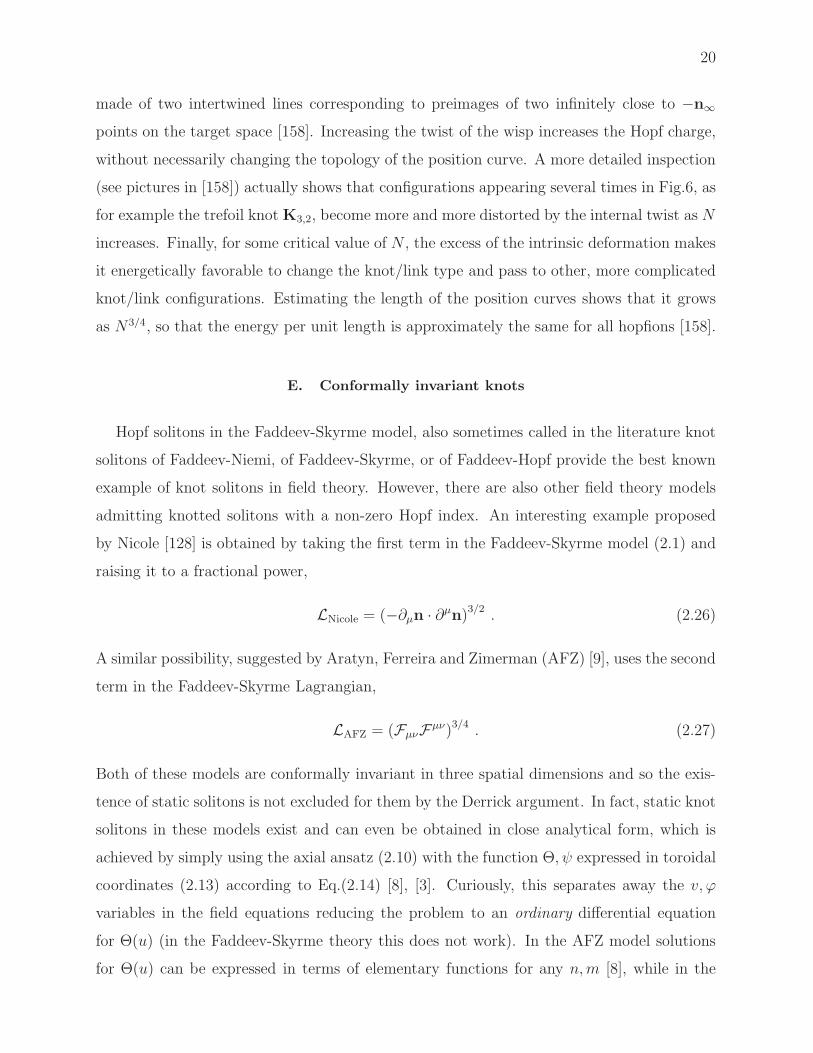
E. Conformally invariant knots
Hopf solitons in the Faddeev-Skyrme model, also sometimes called in the literature knot
solitons of Faddeev-Niemi, of Faddeev-Skyrme, or of Faddeev-Hopf provide the best known
example of knot solitons in field theory. However, there are also other field theory models
admitting knotted solitons with a non-zero Hopf index. An interesting example proposed
by Nicole [128] is obtained by taking the first term in the Faddeev-Skyrme model (2.1) and
raising it to a fractional power,
LNicole = (−∂µn · ∂µn)3/2 . (2.26)
A similar possibility, suggested by Aratyn, Ferreira and Zimerman (AFZ) [9], uses the second
term in the Faddeev-Skyrme Lagrangian,
LAFZ = (FµνFµν)3/4 . (2.27)
Both of these models are conformally invariant in three spatial dimensions and so the exis-
tence of static solitons is not excluded for them by the Derrick argument. In fact, static knot
solitons in these models exist and can even be obtained in close analytical form, which is
achieved by simply using the axial ansatz (2.10) with the function Θ, ψ expressed in toroidal
coordinates (2.13) according to Eq.(2.14) [8], [3]. Curiously, this separates away the v, ϕ
variables in the field equations reducing the problem to an ordinary differential equation
for Θ(u) (in the Faddeev-Skyrme theory this does not work). In the AFZ model solutions
for Θ(u) can be expressed in terms of elementary functions for any n,m [8], while in the

21
Nicole model they are obtained numerically [3], apart from the |n| = |m| = 1 case, where
the solution turns out to be the same in both models and is given by tan(Θ/2) = sinh u
[128], [9]. These results remain, however, interesting mainly from the purely mathematical
point of view at the time being, since it is difficult to justify physically the appearance of
the fractional powers in Eqs.(2.26),(2.27).
Other examples of solitons with a Hopf charge will be discussed below in Sec.VIC and
Sec.VIIC2.
F. Can one gauge the knot solitons ?
The Faddeev-Skyrme theory is a global field model, so that it cannot be a fundamental
physical theory like gauge field theory models, but perhaps can be viewed as an effective
theory. This suggests using the Faddeev-Skyrme knots for an effective description of some
physical objects, and so it has been conjectured by Faddeev and Niemi that they could be
used for an effective description of glueballs in the strongly coupled Yang-Mills theory [66],
[68], [153], [154], [53], [69]. This conjecture is very interesting, quite in the spirit of the
original Lord Kelvin’s idea to view atoms as knotted ether tubes [162], and perhaps it could
apply in some form. In fact, when describing the η(1440) meson, the Particle Data Group
says (see p.591 in Ref.[60]) that “the η(1440) is an excellent candidate for the 0−+ glueball
in the flux tube model [69]”.
Some other physical applications of the global field theory knot solitons could perhaps
be found. However, if they could be promoted to gauge field theory solutions, then they
would be much more interesting physically, since in this case they would find many inter-
esting applications, as for example in the theories of superconductivity and of Bose-Einstein
condensation [11], [12], in the theory of plasma [67], [63], in Standard Model [36], [70],
[130], or perhaps even in cosmology, where they could presumably describe knotted cosmic
strings [165]. For this reason it has been repeatedly conjectured in the literature that some
analogs of the Faddeev-Skyrme knot solitons could also exist as static solutions of the gauge
field theory equations of motion. This conjecture is essentially inspired by the fact that the
Faddeev-Skyrme theory already contains something like a gauge field: Fµν . Moreover, we
shall now see that changing the variables one can rewrite the theory in such a form that it
looks almost identical to a gauge field theory (or the other way round).

22
G. Faddeev-Skyrme model versus semilocal Abelian Higgs model
Let Φ be a doublet of complex scalar fields satisfying a constraint,
Φ =
φ
σ
, Φ†Φ = |φ|2 + |σ|2 = 1, (2.28)
such that Φ ∈ S3. Let us consider a field theory defined by the Lagrangian density
L[Φ] = −1
4FµνFµν + (DµΦ)†DµΦ (2.29)
with Fµν = ∂µAν − ∂νAµ and DµΦ = (∂µ − iAµ)Φ and with
Aµ = −iΦ†∂µΦ . (2.30)
In fact, this theory is again the Faddeev-Skyrme model but rewritten in different variables,
since upon the identification
na = Φ†τaΦ (2.31)
(τa being the Pauli matrices) the fields Aµ and Fµν coincide with those in (2.1) [141] and
the whole action (2.29) reduces (up to an overall factor) to (2.1) [65]. More precisely, (2.31)
is the Hopf projection from S3 parametrized by (φ, σ) to S2 parametrized by the complex
projective coordinate φ/σ. For example, the axially symmetric fields (2.10), (2.11) are
obtained in this way by choosing the CP 1 variables
φ = cosΘ
2einψ, σ = sin
Θ
2eimϕ, (2.32)
such that the phases of φ and σ wind, respectively, along the two orthogonal direction as
shown in Fig.2 and the Hopf charge is N = nm.
The fields in the static limit, Φ = Φ(x), can now be viewed as maps S3 → S3, but their
energy
E[Φ] =
∫(
|DkΦ|2 +1
4(Fik)2
)
d3x (2.33)
is still bounded from below as in Eq.(2.18). The topological charge N = N [Φ], still expressed
by Eq.(2.9), is now interpreted as the index of map S3 → S3, N ∈ π3(S3) = Z. The theory
therefore admits the same knot solitons as the original Faddeev-Skyrme model. However, in
the new parametrization the theory looks almost like a gauge field theory, in particular it
exhibits a local U(1) gauge invariance under Φ→ eiαΦ, Aµ → Aµ + ∂µα.

23
Let us now compare the model (2.29) to a genuine gauge field theory with the Lagrangian
density
L[Φ, Aµ] = −1
4FµνF
µν + (DµΦ)†DµΦ− λ
4(Φ†Φ− 1)2 . (2.34)
Here Φ is again a doublet of complex scalar fields, but this time without the normalization
condition (2.28), the condition (2.30) being also relaxed, so that Aµ is now an independent
field. One has Fµν = ∂µAν − ∂νAµ and DµΦ = (∂µ − iAµ)Φ. This semilocal [2] Abelian
Higgs model with the SU(2)global×U(1)local internal symmetry arises in different contexts,
in particular it can be viewed as the Weinberg-Salam model in the limit where the weak
mixing angle is π/2 and the SU(2) gauge field decouples. The non-relativistic limit of this
theory is the two-component Ginzburg-Landau model [77].
Let us now consider the limit λ → ∞. In this sigma model limit the constraint (2.28)
is enforced and the potential term in (2.34) vanishes. The theories (2.29) and (2.34) then
look identically the same, the only difference being that in the first case the vector field Aµis defined by Eq.(2.30) and so is composite, while in the second case Aµ in an independent
field.
H. Energy bound in the Abelian Higgs model
The question now arises: does the gauge field theory (2.34), at least in the limit where
Φ†Φ = 1, admit knot solitons analogues to those of the global model (2.29) ? If exist, such
solutions would correspond to minima of the energy in the theory (2.34) in static, purely
magnetic sector,
E[Φ, Ak] =
∫(
|DkΦ|2 +1
4(Fik)
2
)
d3x . (2.35)
At first thought, one may think that the answer to this question should be affirmative.
Indeed, the energy functionals (2.33) and (2.35) look identical. They have the same internal
symmetries and the same scaling behaviour under x→ Λx. The two theories also have the
same topology associated to the field Φ, since in both cases Φ(x) defines a mapping S3 → S3
with the topological index (2.9).
The gauged model (2.35) contains in fact even more charges than the global theory (2.33),
since it actually has two vector fields: the independent gauge field Ak and the composite
field Ak = i2(∂kΦ
†Φ− Φ†∂kΦ). It is convenient to introduce their difference Ck = Ak −Ak.

24
Defining the linking number between two vector fields,
I[A,B] =1
4π2
∫
ǫijkAi∂jBk d3x , (2.36)
one can construct three different charges,
N [Φ] ≡ I[A,A], L = I[C,A], NCS[A] ≡ I[A,A], (2.37)
which are, respectively, the topological charge (2.9), the linking number between Ak and Ck,
and the Chern-Simons number of the gauge field. The following inequality, established by
Protogenov and Verbus [137], holds:
E[Φ, Ak] ≥ c1|N |3/4(
1− |L||N |
)2
, (2.38)
where c1 is a positive constant. This can be considered as the generalization of the topological
bound (2.18) of Vakulenko-Kapitanski.
Given all these, one may believe that the local theory (2.35) admits topologically stable
knot solitons similar to those of the global theory (2.33).
I. The issue of charge fixing
The difficulty with implementing the Protogenov-Verbus bound (2.38) in practice is that
it contains two different charges, N and L, but without invoking additional physical assump-
tions there is no reason why L should be fixed while minimizing the energy.
Let us consider first the charge N = N [Φ]. Its variation vanishes identically, so that
it does not change under smooth deformations of Φ. It is therefore a genuine topological
charge whose value is completely determined by the boundary conditions, and so it should
be fixed when minimizing the energy.
Let us now consider the linking number L=I[C,A]. The analogs of this quantity have been
studied in the theory of fluids, where they are known to be integrals of motion [178]. In the
context of gauge field theory, this quantity is gauge invariant. However, it is not a topological
invariant, since its variation does not vanish identically and so it does change under arbitrary
smooth deformations of Ck = Ak − Ak. On cannot fix L using only continuity arguments,
because there are no topological conditions imposed on Ak, whose arbitrary deformations
are allowed. The only topological quantity associated to Ak could be a magnetic charge

25
related to a non-trivial U(1) bundle structure. However, since we are interested in globally
regular solutions, the bundle base space is R3 (or S3) without removed points, in which case
the bundle is trivial.
As a result, on continuity grounds only, one can fix N but not L. But then, as is obvious
from Eq.(2.38), there is no non-trivial lower bound for the energy, since one can always
choose L=N in which case the expression on the right in (2.38) vanishes. More precisely,
since there are no constraints for Ak, nothing prevents one from smoothly deforming it to
zero, after which one can scale away the rest of the configuration. Explicitly, given fields
Φ, Ak one can reduce E[Φ, Ak] to zero via a continues sequence of smooth field deformations
preserving the value of the topological charge N [Φ],
E[Φ(x), Ak(x)]→ E[Φ(Λx), γAk(x)] (2.39)
by taking first the limit γ → 0 and then Λ→∞ [74].
The conclusion is that without constraining Ak, with only N [Φ] fixed, the absolute min-
imum of E[Φ, Ak] is zero, so that there can be no absolutely stable knots. To have such
solutions, one would need to constraint somehow the vector field Ak, for example it would
be enough to insure that Ck = Ak −Ak be zero or small. Such a condition is often assumed
in the literature [12], [11], [36], [70], but usually simply ad hoc. Unfortunately, it cannot be
justified on continuity grounds only, without an additional physical input.
J. Searching for gauged knots
The above arguments do not rule out all solutions in the theory. Even though the global
minimum of the energy is zero, there could still be non-trivial local minima or saddle points.
The corresponding static solutions would be metastable or unstable. One can therefore
wonder whether such solutions exist. This question has actually a long history, being first
addressed by de Vega [49] and by Huang and Tipton [93] over 30 years ago, and being then
repeatedly reconsidered by different authors [109], [130], [74], [174], [95], [57], [55], [56].
However, the answer is still unknown. No solutions have been found up to now, neither has
it been shown that they do not exist.
Trying to find the answer, all the authors were minimizing the energy given by the sum
of E[Φ, Ak] and of a potential term that can be either of the form contained in (2.34) or

26
a more general one. A theory with two vector fields with a local U(1)×U(1) invariance –
Witten’s model of superconducting strings [177] – has also been considered in this context
[57], [55], [56]. The energy was minimized within classes of fields with a given topological
charge N and having profiles of a loop of radius R. The resulting minimal value of energy
was always found to be a monotonously growing function of R, thus always showing the
tendency of the loop to shrink thereby reducing its energy.
These results render the existence of solutions somewhat implausible. However, they do
not yet prove their absence. Indeed, local energy minima may be difficult to detect via energy
minimization, as this would require starting the numerical iterations in their close vicinity,
because otherwise the minimization procedure converges to the trivial global minimum. In
other words, one has to choose a good initial configuration. However, since ‘there is a lot of
room in function space’, chances to make the right choice are not high.
It should be mentioned that a positive result was once reported in Ref.[130], were the
energy was minimized in the N = 2 sector and an indication of a convergence to a non-trivial
minimum was observed. However, this result was not confirmed in an independent analysis
in Ref.[174], so that it is unclear whether it should be attributed to a lucky choice of the
initial configuration or to some numerical artifacts.
III. KNOT SOLITONS IN GAUGE FIELD THEORY
As we have seen, fixing only the topological charge does not guarantee the existence of
knot solitons in gauge field theory. In order to obtain such solutions one needs to constraint
the gauge field in order that it could not be deformed to zero. Below we describe two known
examples of such solutions.
A. Anomalous solitons
One possibility to constraint the gauge field is to fix its Chern-Simons number. An
example of how this can be done was suggested long ago by Rubakov and Tavkhelidze [143],
[142], who showed that the Chern-Simons number can be fixed by including fermions into
the system. They considered the Abelian Higgs model (2.34), but with a singlet and not
doublet Higgs field, augmented by including chiral fermions. In the weak coupling limit

27
at zero temperature this theory contains states with NF non-interacting fermions and with
the bosonic fields being in vacuum, Aµ = 0, Φ = 1. The energy of such states is E ∼ NF .
Rubakov and Tavkhelidze argued that this energy could be decreased via exciting the bosonic
fields in the following way.
Owing to the axial anomaly, when the gauge field Aµ varies, the fermion energy levels
can cross zero and dive into the Dirac see. The fermion number can therefore change, but
the difference NF − NCS is conserved. As a result, starting from a purely fermionic state
and increasing the gauge field, one can smoothly deform this state to a purely bosonic state,
whose Chern-Simon number will be fixed by the initial conditions,
NCS = NF . (3.40)
Now, the energy of this state,
E[Φ, Ak] =
∫(
|DkΦ|2 +1
4(Fik)
2 +λ
4(|Φ|2 − 1)2
)
d3x , (3.41)
can be shown to be bounded from above by E0(NCS)3/4 where E0 is a constant, and so for
large NF = NCS it grows slower than the energy of the original fermionic state, E ∼ NCS
[143], [142]. Therefore, for large enough NF , it is energetically favorable for the original
purely fermionic state to turn into a purely bosonic state. The latter is called anomalous
[143], [142]. The energy of this anomalous state can be obtained by minimizing the functional
(3.41) with the Chern-Simons number fixed by the condition (3.40).
Such an energy minimization was carried out in the recent work of Schmid and Shaposh-
nikov [151]. First of all, they established the following inequality,
E[Φ, Ak] ≥ c(NCS)3/4, (3.42)
which reminds very much of the Vakulenko-Kapitanski bound (2.18) for the Faddeev-Skyrme
model, but with the topological charge replaced by NCS. This gives a very good example of
how constraining the gauge field can stabilize the system: even though in the theory with a
singlet Higgs field there is no topological charge similar to the Hopf charge, its role can be
taken over by the Chern-Simons charge.
In order to numerically minimize the energy, Schmid and Shaposhnikov considered the
Euler-Lagrange equations for the functional
E[Φ, Ak] + µ
∫
ǫijkAi∂jAkd3x (3.43)

28
ρ
R
s
sφ
φ
=0
=1 Ak=0
Ak=0
x
z
FIG. 7: Spindle torus shape of the anomalous solitons for large NCS.
where E[Φ, Ak] is given by (3.41) and µ is the Lagrange multiplier. In the gauge where
Φ = Φ∗ ≡ φ these equations read (with ~A = Ak)
∆φ− ~A 2φ− λ
2(φ2 − 1)φ = 0, (3.44a)
~∇× (~∇× ~A) + 2µ~∇× ~A + 2φ2 ~A = 0, (3.44b)
where ~∇ and ∆ = (~∇)2 are the standard gradient and Laplace operators, respectively.
Multiplying Eq.(3.44b) by ~A and integrating gives the expression for the Lagrange multiplier,
µ =1
32π2NCS
∫(
(∇× ~A)2 + | ~A|2φ2
)
d3x. (3.45)
Solutions of the elliptic equations (3.44a),(3.44b) were studied in [151] in the axially sym-
metric sector, where φ = φ(ρ, z) and ~A = ~A(ρ, z), with the boundary conditions
φ = 1, ~A = 0 (3.46)
at infinity and
∂ρφ = ∂ρAz = 0, Aρ = Aϕ = 0 (3.47)
at the symmetry axis ρ = 0. The solutions obtained are quite interesting. They are very
strongly localized in a compact region, Ω, of the (ρ, z) plane centered around a point (ρs, 0).
Inside Ω the field Ak is non-zero, while φ is almost constant and very close to zero. As
one approaches the boundary of the region, ∂Ω, the field Ak tends to zero, while φ is still
almost zero. Finally, in a small neighborhood of ∂Ω whose thickness is of the order of the
Higgs boson wavelength, φ starts varying and quickly increases up to its asymptotic value.
Outside Ω one has everywhere φ ≈ 1 and Ak ≈ 0, such that the energy density is almost

29
zero. The energy for these solutions scales as (NCS)3/4. For large NCS the region Ω can be
described by the simple analytic formula,
(ρ− ρs)2 + z2 < R2s , (3.48)
where Rs > ρs. In other words, the 3D domain where the soliton energy is concentrated can
be obtained by rotating around the z-axis a disc centered at a point whose distance from the
z-axis is less than its radius (see Fig.7). Such a geometric figure is called spindle torus [151].
The solutions for large NCS are very well approximated by setting φ = 1 and Ak = 0 outside
the spindle torus, while inside it one has φ = 0 and Ak is obtained by solving the linear
equation (3.44b). The spindle torus approximation becomes better and better for large NCS,
in which limit Schmid and Shaposhnikov obtain the following asymptotic formulas for the
energy and parameters of the torus, which agree very well with their numerics,
E = 118λ1/4MW (NCS)3/4, ρs =
1.7
MW
(
NCS
λ
)1/4
, Rs = 1.49ρs , (3.49)
where MW is the vector field mass.
It is likely that these solution attain the lower energy bound (3.40), which means that
they should be topologically stable. It should, however, be emphasized that the anomalous
solitons require a rather exotic physical environment, since for them to be energetically
favoured as compared to the free fermion condensate, the density of the latter should attain
enormous values possible perhaps only in the core of neutron stars.
Summarizing, fixing the Chern-Simons number forbids deforming the gauge field to zero
and gives rise to stable knot solitons in gauge field theory, even if the Higgs field is topolog-
ically trivial. It is unclear whether this result can be generalized within the context of the
model (2.34) with two component Higgs field – since the Protogenov-Verbus formula (2.38)
contains not the Chern-Simons number but the linking number L.
B. Non-Abelian rings
Another interesting class of objects arises in the non-Abelian gauge field theory, where
one can have smooth, finite energy loops stabilized by the magnetic energy.
30
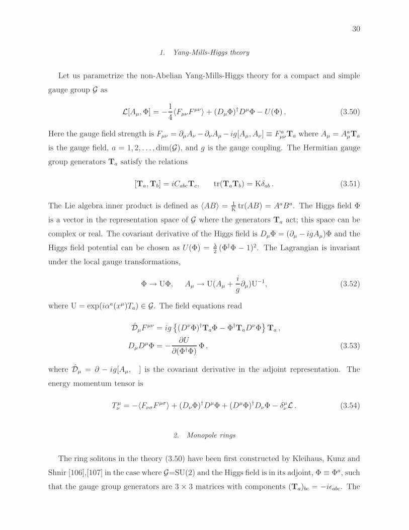
1. Yang-Mills-Higgs theory
Let us parametrize the non-Abelian Yang-Mills-Higgs theory for a compact and simple
gauge group G as
L[Aµ,Φ] = −1
4〈FµνF µν〉+ (DµΦ)†DµΦ− U(Φ) . (3.50)
Here the gauge field strength is Fµν = ∂µAν −∂νAµ− ig[Aµ, Aν ] ≡ F aµνTa where Aµ = AaµTa
is the gauge field, a = 1, 2, . . . , dim(G), and g is the gauge coupling. The Hermitian gauge
group generators Ta satisfy the relations
[Ta,Tb] = iCabcTc, tr(TaTb) = Kδab . (3.51)
The Lie algebra inner product is defined as 〈AB〉 = 1K
tr(AB) = AaBa. The Higgs field Φ
is a vector in the representation space of G where the generators Ta act; this space can be
complex or real. The covariant derivative of the Higgs field is DµΦ = (∂µ − igAµ)Φ and the
Higgs field potential can be chosen as U(Φ) = λ2
(Φ†Φ − 1)2. The Lagrangian is invariant
under the local gauge transformations,
Φ→ UΦ, Aµ → U(Aµ +i
g∂µ)U
−1, (3.52)
where U = exp(iαa(xµ)Ta) ∈ G. The field equations read
DµF µν = ig
(DνΦ)†TaΦ− Φ†TaDνΦ
Ta ,
DµDµΦ = − ∂U
∂(Φ†Φ)Φ , (3.53)
where Dµ = ∂ − ig[Aµ, ] is the covariant derivative in the adjoint representation. The
energy momentum tensor is
T µν = −〈FνσF µσ〉+ (DνΦ)†DµΦ + (DµΦ)†DνΦ− δµνL . (3.54)
2. Monopole rings
The ring solitons in the theory (3.50) have been first constructed by Kleihaus, Kunz and
Shnir [106],[107] in the case where G=SU(2) and the Higgs field is in its adjoint, Φ ≡ Φa, such
that the gauge group generators are 3 × 3 matrices with components (Ta)bc = −iǫabc. The

31
fundamental solutions in this theory are the magnetic monopoles of ’t Hooft and Polyakov
[160],[136], while the ring solitons are more general solutions. Specifically, in the static,
axially symmetric and purely magnetic case it is consistent to choose the following ansatz
for the fields in spherical coordinates:
Aµdxµ = (K1dr + (1−K2)dϑ)Tϕ +m(K3Tr + (1−K4)Tϑ) sinϑ dϕ,
TaΦa = φ1Tr + φ2Tϑ , (3.55)
where functions K1, K2, K3, K4, φ1, φ2 depend on r, ϑ and are subject of suitable boundary
conditions at the symmetry axis and at infinity [106],[107]. Here
Tr = sin(kϑ) cos(mϕ)T1 + sin(kϑ) sin(mϕ)T2 + cos(kϑ)T3,
Tϑ =1
k
∂
∂ϑTr , Tϕ =
1
m sin ϑ
∂
∂ϕTr , (3.56)
with k,m ∈ Z. Using the gauge invariant tensor
Fµν = ΦaF aµν − ǫabcΦaDµΦ
bDνΦc (3.57)
and its dual, Fµν = 12ǫµναβFαβ, one can define the electric and magnetic currents, respec-
tively, as
jµ = ∂αFαµ, jµ = ∂αFαµ . (3.58)
It turns out that the solutions depend crucially on values of k,m in (3.55). In particular,
their magnetic charge is given by
Q =m
2[1− (−1)k]. (3.59)
The following solutions are known in the limit of vanishing Higgs potential (for a generic
potential their structure is more complicated) [106],[107]:
k = 1, m = 1 – the spherically symmetric ’t Hooft-Polyakov monopole.
k = 1, m > 1 – multimonopoles.
k > 1, m = 1, 2 – monopole-antimonopole sequences.
k = 2l ≥ 2, m ≥ 3 – monopole vortex rings.
In the first three cases the Higgs field has discrete zeros located at the z-axis. Solutions of the
last type are especially interesting in the context of our discussion, since zeros of the Higgs
fields in this case are not discrete but continuously distributed along a circle (for k = 2)

32
0 0.1 0.2 0.3 0.4 0.5 0.6 0.7 0.8 0.9
0
3
6
9
12
15
ρ
-15-10
-5 0
5 10
15
z
0
0.25
0.5
0.75
|φ|
−P
j
Bj
BP
+P
FIG. 8: Left: Higgs field amplitude for the k = 2, m = 3 monopole ring solution in the limit
where the Higgs field potential is zero. |Φ| vanishes at a point in the (ρ, z) plane away from the
z-axis, which corresponds to a ring. Right: schematic shape of charge/current distribution for this
solution.
around the z-axis (see Fig.8). Solutions in this case can be visualized as stationary rings
stabilized by the magnetic energy. The mechanism of their stabilization is quite interesting
and can be elucidated as follows [155, 156]. If one studies the profiles of the currents (3.58)
for these solutions, it turns out that both the magnetic charge density j0 and the electric
current density jk have ring shape distributions, as qualitatively shown in Fig.8.
Although the total magnetic charge is zero, locally the charge density is non-vanishing
and the system can be visualized as a pair of magnetically charged rings with opposite charge
located at z = ±z0, accompanied by a circular electric current in the z = 0 plane. The two
magnetic rings create a magnetic field orthogonal to the z = 0 plane. This magnetic field
forces the electric charges in the plane to Larmore orbit, which creates a circular current.
The Biot-Savart magnetic field produced by this current acts, in its turn, on the magnetic
rings keeping them away from each other, so that the whole system is in a self-consistent
equilibrium [155] (assuming the magnetic rings to be rigid).
It is, however, unlikely that this sophisticated balance mechanism stabilizing the rings
against contraction could also guarantee their stability with respect to all possible deforma-
tions. In fact, the monopole-antimonopole solution is known to be unstable [161], while the
monopole rings can be viewed as generalizations of this solution. They are therefore likely
to be saddle points of the energy functional and so they should be unstable as well.

33
3. Sphaleron rings
Very recently, a similar ring construction was carried out by Kleihaus, Kunz and Leissner
[101] within the context of the Yang-Mills-Higgs theory (3.50) with G=SU(2) and with the
Higgs field in its fundamental complex doublet representation, where Ta = 12τa. This theory
can be viewed as the SU(2)×U(1) Weinberg-Salam theory in the limit where the weak mixing
angle vanishes and the U(1) gauge field decouples. Kleihaus, Kunz and Leissner used exactly
the same field ansatz (3.55), only modifying the Higgs field as
Φ = (φ1Tr + φ2Tϑ)Φ0 , (3.60)
where Φ0 is a constant 2-vector. As in the monopole case, in this case too the solutions
depend strongly on the choice of the integers k and m in Eq.(3.56). The fundamental
solutions in this case are the sphalerons – unstable saddle point configurations that can be
smoothly deformed to vacuum. They can be characterized by the Chern-Simons number,
given by the same formula as the magnetic charge in the monopole case, up to the factor
1/2, so that half-integer values are now allowed: Q = m[1− (−1)k]/4.
Setting k = m = 1 gives the Klinkhamer-Manton sphaleron [108], in which case the Higgs
field vanishes at one point. Choosing k = 1, m > 1 or k > 1, m = 1 gives multisphalerons or
sphaleron-antisphaleron solutions for which the Higgs field has several isolated zeros located
at the symmetry axis [101]. A new type of solution arises for k ≥ 2, m ≥ 3, in which case
the Higgs field vanishes on one or more rings centered around the symmetry axis. In this
respect these sphaleron rings are quite analogues to the monopole rings. It is unclear at the
moment whether their existence can be qualitatively explained by a mechanism similar to
that for the monopole rings, shown in Fig.8.
Since sphalerons are unstable objects, it is very likely that sphaleron rings are also un-
stable. However, similar to the sphalerons, they could perhaps be interesting physically as
mediators of baryon number violating processes [108].
IV. ANGULAR MOMENTUM AND RADIATION IN FIELD SYSTEMS
We are now passing to the spinning systems with the ultimate intention to discuss spin-
ning vortex loops stabilized by the centrifugal force – vortons. As was already said in the
Introduction, usually vortons are considered within a qualitative macroscopic description as

34
loops made of vortices and stabilized by rotation. This description is suggestive, but it does
not take into account the radiation damping. At the same time, the presence of the vorton
angular momentum requires some internal motions in the system (see Fig.9), as for example
circular currents, and these are likely to generate radiation carrying away both the energy
and angular momentum. It is therefore plausible that macroscopically constructed vortex
loops will not be stationary field theory objects, but at best only quasistationary, with a
finite lifetime determined by the radiation rate.
Pj
j P
J
supe
rcon
duct
ing
stri
ng
vorton
JRADIATION ?
Pvorton
j
FIG. 9: One can make a loop from a vortex carrying a current j and momentum P . It will have
an angular momentum, but it may be radiating.
The best way to decide whether vortons are truly stationary or only quasistationary is
to explicitly resolve the corresponding field theory equations. The current situation in this
direction is not, however, very suggestive. Within the original local U(1)×U(1) Witten’s
model of superconducting cosmic strings [177] vorton solutions have never been constructed.
To the best of our knowledge, the only explicit vorton solutions have been presented by
Lemperier and Shellard [118] within the global version of Witten’s model, and also by
Battye, Cooper and Sutcliffe [17] in a special limit of the same global model. In addition,
vortons in a 2 + 1 dimensional field theory toy model have been recently analyzed [19].
Lemperier and Shellard [118] considered the full hyperbolic evolution problem for the
fields, with the initial data corresponding to a vortex loop. Evolving dynamically this loop
in time, they saw it oscillate around a visibly stationary equilibrium position, and they could
follow these oscillations for several dozens characteristic periods of the system. This suggests
that vortons exist and are stable against perturbations. However, one cannot decide on these
grounds whether the equilibrium configurations are truly stationary or only quasistationary,
since the radiation damping could be non-zero but too small to be visible in their numerics.
In addition, Lemperier and Shellard did not actually consider precisely the global version

35
of Witten’s model (see Eq.(6.138) below), but, in order to improve the numerics, added to
it a Q-ball type interaction term of the form |φ|6|σ|2, where φ, σ are the two scalars in the
model.
Battye, Cooper and Sutcliffe [17] did not study Witten’s model but minimized the energy
of a non-relativistic Bose-Einstein condensate, which seems to be mathematically equivalent
to solving equations of Witten’s model in a special limit. They found non-trivial energy
minima saturated by configurations of vorton type, which again suggests that vortons exist,
at least in this limit. Moreover, this suggests that they are indeed non-radiative – since
being already in the energy minimum they cannot loose energy anymore. It would therefore
be interesting to construct these solutions in a different way, extending the analysis to the
full Witten’s model.
The method we shall employ below to study truly non-radiating vortons will be to con-
struct them as stationary solutions of the elliptic boundary value problem obtained by
separating the time variable. However, first of all we need to understand how in principle
a non-radiating field system can have a non-zero angular momentum. Both angular mo-
mentum and radiation are associated to some internal motions in the system, and it is not
completely clear how to reconcile the presence of the former with the absence of the latter.
A. Angular momentum for stationary solitons
In what follows we shall be considering field theory systems obeying the following four
conditions:
(1) stationarity
(2) finiteness of energy
(3) axial symmetry
(4) non-vanishing angular momentum
The angular momentum is defined as the Noether charge associated to the global space-
time symmetry generated by the axial Killing vector K = ∂/∂ϕ,
J =
∫
T 0ϕd
3x . (4.61)
Let us discuss the first three conditions.
(1) A system is stationary if its energy momentum tensor T µν does not depend on time.

36
According to the standard definition of symmetric fields [71], for stationary fields the action
of time translations can be compensated by internal symmetry transformations.
If all internal symmetries of the theory are local, then there is a gauge where the compen-
sating symmetry transformation is trivial, so that the stationary fields are time-independent.
We shall call them manifestly stationary. If the theory contain also global internal symme-
tries and if the compensating symmetry transformation is global, then its action cannot be
trivialized and so the action of time translations will be non-trivial. The fields will explicitly
depend on time in this case, typically via time-dependent phases, and we shall call them
non-manifestly stationary.
For example, in a system with two complex scalars coupled to a U(1) gauge field one
cannot gauge away simultaneously phases of both scalars. A non-manifestly stationary field
configuration will then be φ1(x), φ2(x)eiωt, Aµ(x). However, if there is only one scalar, then
it is always possible to gauge away its time-dependent phase.
(2) Even if T µν is time-independent, one can still have a constant radiation flow compen-
sated by the energy inflow from infinity. However, if the energy is finite, then the fields
fall-off fast enough at infinity to eliminate this possibility.
In principle, one can also have situations where T µν is time-dependent, but radiation is
nevertheless absent, as for the breathers in 1+1 dimensions [139]. However, such cases are
probably less typical and we shall not discuss them.
(3) It is intuitively clear that asymmetric spinning systems will more likely radiate than
symmetric ones. It is therefore most natural to assume spinning non-radiating solitons to
be axially symmetric. The axially symmetry can be manifest or non-manifest. In fact, it
appears that the axial symmetry condition can sometimes be relaxed, but such a possibility
seems to be more exotic and will be discussed below only very briefly in Sec.VC.
Let us now analyze possibilities for condition (4) to coexist with (1)–(3).
1. The case of manifest symmetries – no go results
In theories where all internal symmetries are local the stationary field are time-
independent. Can one have an angular momentum in this case ?
In fact, even without an explicit time dependence one can have a non-vanishing field
momentum expressed by the Poynting vector, ~E × ~B, and this could give a contribution to

37
the angular momentum,∫
~r × (~E × ~B) d3x . (4.62)
If the theory contains gauged scalars, they will give an additional contribution. If there exists
a stationary, globally regular, finite energy on-shell configuration for which the integral (4.61)
is non-zero, this would correspond to a rotating and non-radiating soliton. The existence of
such solutions is not a priori excluded. However, it turns out that for a number of physically
interesting cases they can be ruled out.
Specifically, since the time translations and spatial rotations commute, the system is not
only manifestly stationary but also manifestly axially symmetric [71]. It turns out that
the latter condition allows one to transform the volume integral in Eqs.(4.61) to a surface
integral, which is often enough to conclude that J = 0.
To me more precise, let us consider the Yang-Mills-Higgs theory (3.50). If the fields
(Aµ,Φ) are manifestly invariant under the action of a Killing symmetry generatorK = ∂/∂s,
then there is a gauge where they do not depend on the corresponding spacetime coordinate
s and their Lie derivatives along K vanish, LKAµ = LKΦ = 0. In some other gauge the
fields could depend on s, but only in such a way that [71]
LKAµ = DµW (K) , LKΦ = igW (K)Φ . (4.63)
Here W (K) takes its values in the Lie algebra of the gauge group and transforms as connec-
tion under gauge transformations. If K = ∂/∂ϕ is the axial Killing vector and Wϕ ≡W (K),
then in spherical coordinates these conditions reduce to
∂ϕAµ = DµWϕ , ∂ϕΦ = igWϕΦ . (4.64)
If these conditions are fulfilled, then it is straightforward to check with the field equations
(3.53) that the T 0ϕ component of the energy-momentum tensor (3.54) has a total derivative
structure [50], [169],
T 0ϕ = ∂k〈(Wϕ − Aϕ)F 0k〉 . (4.65)
Since both Aϕ and Wϕ transform as connections under gauge transformations, their differ-
ence is gauge covariant, so that this formula is gauge invariant. For globally regular solutions
the electric field Ek = F 0k is everywhere bounded, which allows one to transform the volume
integral of T 0ϕ to a surface integral over the boundary of R3 at infinity. This gives the surface

38
integral representation for the angular momentum
J =
∮
〈(Wϕ − Aϕ)~E〉 ~dS . (4.66)
This formula imposes rather strong restrictions on the existence of spinning solitons. For
example, it shows that if the electric field E decays at infinity faster than 1/r2, such that
the electric charge is zero, then J = 0. A non-zero electric charge is therefore necessary to
have a non-zero angular momentum [50]. Similarly, using the asymptotic conditions in the
far field zone, one can show that for a number of important cases the asymptotic behavior
of the fields does not allow for the surface integral to be non-zero.
FIG. 10: Do static solitons admit stationary, spinning generalizations ?
Specifically, one can consider any known static, spherically symmetric soliton, as for
example the ’t Hooft-Polyakov monopole, and ask if it admits stationary, spinning general-
izations (see Fig.10) ? For example, the static Schwarzschild black hole solution of Einstein’s
equation in General Relativity can be generalized to the manifestly stationary, spinning Kerr
black hole. One can wonder if similar generalizations are possible for solitons in non-linear
field theories in Minkowski space. If they exist, then in the far field zone their fields should
approach those of the original static soliton, so that they should be spherically symmetric,
up to small corrections which could contribute to the surface integral (4.66). Since the
corrections are small, their most general form can be determined from the linearized field
equations [169].
Surprisingly, one discovers in this way that none of the well known solitons in the gauge
field theory (3.50) with gauge group SU(2), as for example the magnetic monopoles of
’t Hooft-Polyakov [160], [136], dyons of Julia-Zee [98], and sphalerons of Klinkhamer-Manton

39
[108], admit spinning generalizations within the manifestly stationary and manifestly ax-
isymmetric sector [50], [51], [169]. The picture in Fig.10 thus does not apply for these
solitons. If the gauge symmetry is completely broken in the Higgs vacuum, as for the
sphalerons, then the fields approach their vacuum values exponentially fast and the surface
integral vanishes. For the monopoles and dyons there is a long-range field associated with
the unbroken U(1), so that some additional analysis is required to show that in the asymp-
totic region there are actually no field modes giving a non-zero contribution to the surface
integral [169].
As a result, the best known SU(2) solitons cannot spin in the manifestly stationary and
manifestly axisymmetric sector. This restricts rather strongly the existence of spinning soli-
tons with manifest symmetries, although does not rule them out completely. Such solutions
might exist in theories with other gauge groups. Their explicit examples in U(1) gauge field
theories will be presented below. Non-manifestly symmetric rotational excitations could
perhaps exist for the sphalerons, since only an SU(2) part of their U(2) internal symmetry is
gauged. A more exotic possibility to have stationary rotation without axial symmetry will
be briefly discussed in Sec.VC.
2. The case of non-manifest symmetries
More general possibilities to have spinning solitons arise in theories where not all internal
symmetries are local, since in this case the conditions (4.63) can be generalized as
LKAµ = DµW (K) , LKΦ = igW (K)Φ + iT (K)Φ , (4.67)
where T (K) is a function of the global symmetry generators. One can gauge away W (K)
but not T (K), so that the action of the Killing symmetry will always be non-trivial, since
Φ will depend explicitly on the corresponding spacetime coordinate s as
Φ(s) = eisT (K)Φ0 . (4.68)
This means that the s-dependence is equivalent to a sequence of internal symmetry trans-
formations, in which case the invariant objects like T µν will not depend on s at all. Such
a symmetry can be called non-manifest. Non-manifestly stationary and non-manifestly ax-
isymmetric fields would typically depend on t, ϕ via the complex phase factor
expi(ωt+mϕ), (4.69)
40
in which case one can say that it is the phase that spins. The angular momentum in this
case cannot be totally expressed by a surface integral and will contain a volume integral
contribution, in which case typically J ∼ ωm.
As a result, one can have J 6= 0. However, the absence of radiation is not yet guaranteed.
Separating the time variable makes the equations elliptic, but with the mass term(s) modified
as
M2 →M2 − ω2, (4.70)
where M2 collectively denotes masses of the field excitations in the asymptotic zone. Now,
if the equations admit globally regular solutions with
ω2 < M2 (4.71)
then these solutions will behave asymptotically as exp−√M2 − ω2 r and there will be
no radiation. On the other hand, if ω2 > M2 then solutions in the asymptotic region will
oscillate as exp±i√ω2 −M2 r thus showing the presence of the ingoing and outgoing
radiation, even though T µν is time-independent, so that the total energy will be infinite. As
a result, the no-radiation condition (4.71) becomes crucial in this case.
3. Spinning solitons as solutions of elliptic equations
Summarizing the above discussion, one can conclude that the existence of non-radiating
spinning solitons, although not forbidden, is not guaranteed either. Even for known static
solitons their spinning generalizations may or may not exist, and if they do exist, this should
be considered as something exceptional rather than the general rule. At first view, such a
conclusion may seem to contradict our experience, since normally one knows that compact
objects can spin. However, we are not saying that generic field theory solitons cannot spin.
They always can, but it seems that they should generically radiate at the same time. One can
always ‘give a kick’ to any static soliton, as for example to the magnetic monopole or to any
of the knotted solitons of Faddeev-Skyrme shown in Fig.6, so that they will start spinning.
However, at the same time they will start radiating away all the received energy and angular
momentum, till they relax back to the original static, non-spinning configuration. It seems
that ‘spinning and radiating’ represents the generic way the field systems behave, while
41
‘spinning without radiating’ should rather be considered as something exceptional, possible
only in some special field theory models.
Perhaps the best way to really establish the existence of spinning and non-radiating
solitons would be to construct them as solutions of the elliptic boundary value problem
obtained by separating the time variable. In gauge field theory, as for example in the local
U(1)×U(1) Witten’s model [177], one could look for manifestly stationary and axisymmetric
vortons, in which case there is no radiation. However, since the angular momentum in
this case can be expressed by the surface integral (4.66) and so is determined only by the
asymptotic behavior of the fields, there are higher chances that it could vanish. For global
field theories one could consider systems with non-manifest symmetries, in which cases there
are better chances to have a non-zero angular momentum, but also higher chances to have
radiation, unless the no-radiation condition (4.71) is fulfilled.
V. EXPLICIT EXAMPLES OF STATIONARY SPINNING SOLITONS
Before coming to vortons, one can wonder, in view of the above discussion, if there exist
at all any known examples of non-radiating spinning solitons. As we said, for the SU(2)
magnetic monopoles, dyons and sphalerons there are no spinning generalizations, at least in
the manifestly stationary and manifestly axisymmetric case. Nevertheless, explicit examples
of spinning solitons in Minkowski space in 3 + 1 dimensions exist and below we shall review
all known solutions of this type. These are the spinning Q-balls, spinning Skyrmions and
also rotating monopole-antimonopole pairs, apart from the vortons. Interestingly, it seems
that spinning solitons are in some sense more easily constructed in curved space, because the
spinning degrees of freedom can be naturally associated to the non-radiative dipole moment
of gravitational field. For this reason a number of articles cited below actually describe the
Minkowski space spinning solitons only as a special limit of the more general, self-gravitating
configurations.
A. Q-balls
This is an important for our discussion example which shares many features with the
vortons. At the same time, spinning Q-balls are simpler than vortons, and so they can be

42
used to introduce a number of notions to be applied later. We shall therefore discuss them
in some detail.
Q-balls have been introduced by Coleman [39]. These are non-topological solitons [116]
found in a theory with a single complex scalar field with the Lagrangian density
LQ[Φ] = ∂µΦ∗∂µΦ− U(|Φ|), (5.72)
the corresponding field equation being
∂µ∂µΦ +
∂U
∂|Φ|2 Φ = 0, (5.73)
while the energy-momentum tensor
Tµν = ∂µΦ∗∂νΦ + ∂νΦ
∗∂µΦ− gµνLQ. (5.74)
The potential U should have the absolute minimum, U(0) = 0, and should also satisfy the
condition
ω2− = min
f
U(f)
f 2< ω2
+ =1
2
d2U
df 2
∣
∣
∣
∣
f=0
, (5.75)
whose meaning will be explained below. The value of ω+ determines the mass of the field
quanta, M = ω+. For the condition (5.75) to be fulfilled U should (if it is even in |Φ|) contain
powers of |Φ| higher than four, which means that the theory cannot be renormalizable [39].
A convenient choice is
U = λ|Φ|2(|Φ|4 − a|Φ|2 + b), (5.76)
where λ, a, b are positive constants, so that ω2+ = λb and ω2
− = ω2+(1 − a2/4b). In our
numerics below we shall always choose λ = 1, a = 2, b = 1.1 [168], which is not a restriction
(for ω− 6= 0) since λ, a can be changed by rescaling the coordinates and field, while the
mass M =√λb enters the field equation (5.83) only in the combination M2−ω2 where ω is
another free parameter.
The global invariance of the theory under Φ → Φeiα implies the conservation of the
Noether charge
Q = i
∫
(∂tΦ∗Φ− Φ∗∂tΦ)d3x . (5.77)
The scaling argument of Derrick applies for the theory (5.72) and rules out all static solutions
with finite energy. Therefore, in order to circumvent this argument, solutions should depend
on time,
Φ = φ(x)eiωt, (5.78)

43
in which case the Noether charge is
Q = 2ω
∫
φ2d3x ≡ 2ωN . (5.79)
In what follows we shall assume ω to be positive. More explicitly, with
E2 =
∫
(∇φ)2d3x, E0 =
∫
Ud3x, (5.80)
the Lagrangian reads
L =
∫
LQ d3x = ω2N −E0 − E2. (5.81)
Under scale transformations x → Λx one has L → Λ3(ω2N − E0)− ΛE2 so that L will be
stationary for Λ = 1 if the virial relation is fulfilled,
3ω2N = 3E0 + E2, (5.82)
which is only possible (for E0 6= 0, E2 6= 0) if ω 6= 0.
Q-balls are finite energy solutions of the Lagrangian field equations for the ansatz (5.78),
(
∆ + ω2)
φ =∂U
∂|φ|2 φ. (5.83)
Even though Φ depends on time, Tµν is time independent – the system is non-manifestly
stationary. Equivalently, Q-balls can be obtained by minimizing the total energy
E =
∫
T 00 d
3x =
∫
(ω2|φ|2 + |∇φ|2 + U)d3x ≡ ω2N + E0 + E2 (5.84)
by keeping fixed the charge Q. Indeed, rewriting the energy as
E =Q2
4N + E0 + E2 (5.85)
shows that minimizing E with Q fixed is equivalent to extremizing L, since
δE = − Q2
4N 2δN + δ(E0 + E2) = −ω2δN + δ(E0 + E2) = −δL , (5.86)
so that the on-shell condition δL = 0 follows from δE = 0. It is also instructive to see how
the same thing comes about within the Lagrange multiplier method. Introducing
EQ =
∫
(ω2|φ|2 + |∇φ|2 + U)d3x + µ
(
2ω
∫
|φ|2d3x−Q)
, (5.87)
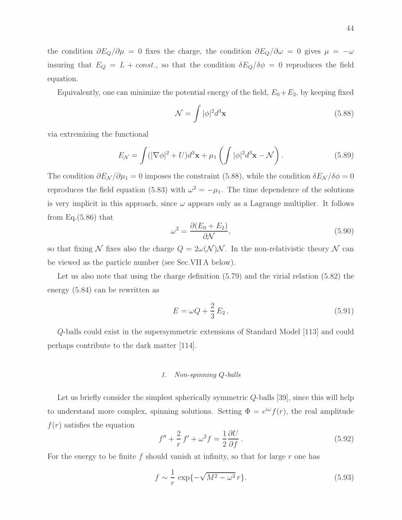
44
the condition ∂EQ/∂µ = 0 fixes the charge, the condition ∂EQ/∂ω = 0 gives µ = −ωinsuring that EQ = L + const., so that the condition δEQ/δφ = 0 reproduces the field
equation.
Equivalently, one can minimize the potential energy of the field, E0+E2, by keeping fixed
N =
∫
|φ|2d3x (5.88)
via extremizing the functional
EN =
∫
(|∇φ|2 + U)d3x + µ1
(∫
|φ|2d3x−N)
. (5.89)
The condition ∂EN /∂µ1 = 0 imposes the constraint (5.88), while the condition δEN/δφ = 0
reproduces the field equation (5.83) with ω2 = −µ1. The time dependence of the solutions
is very implicit in this approach, since ω appears only as a Lagrange multiplier. It follows
from Eq.(5.86) that
ω2 =∂(E0 + E2)
∂N , (5.90)
so that fixing N fixes also the charge Q = 2ω(N )N . In the non-relativistic theory N can
be viewed as the particle number (see Sec.VIIA below).
Let us also note that using the charge definition (5.79) and the virial relation (5.82) the
energy (5.84) can be rewritten as
E = ωQ+2
3E2 . (5.91)
Q-balls could exist in the supersymmetric extensions of Standard Model [113] and could
perhaps contribute to the dark matter [114].
1. Non-spinning Q-balls
Let us briefly consider the simplest spherically symmetric Q-balls [39], since this will help
to understand more complex, spinning solutions. Setting Φ = eiωf(r), the real amplitude
f(r) satisfies the equation
f ′′ +2
rf ′ + ω2f =
1
2
∂U
∂f. (5.92)
For the energy to be finite f should vanish at infinity, so that for large r one has
f ∼ 1
rexp−
√M2 − ω2 r. (5.93)
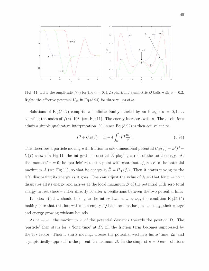
45
-0.5
0
0.5
1
0 5 10 15 20 25 30
r
n = 0n = 0
n = 1n = 1
n = 2n = 2
-0.2
-0.1
0
0.1
0.2
0.3
0.4
-1.5 -1 -0.5 0 0.5 1 1.5
f
f0
f∞ = 0
Ueff
A
BC
D
ω+
ω−
FIG. 11: Left: the amplitude f(r) for the n = 0, 1, 2 spherically symmetric Q-balls with ω = 0.2.
Right: the effective potential Ueff in Eq.(5.94) for three values of ω.
Solutions of Eq.(5.92) comprise an infinite family labeled by an integer n = 0, 1, . . .
counting the nodes of f(r) [168] (see Fig.11). The energy increases with n. These solutions
admit a simple qualitative interpretation [39], since Eq.(5.92) is then equivalent to
f ′2 + Ueff(f) = E − 4
∫ r
0
f ′2 dr
r. (5.94)
This describes a particle moving with friction in one-dimensional potential Ueff(f) = ω2f 2−U(f) shown in Fig.11, the integration constant E playing a role of the total energy. At
the ‘moment’ r = 0 the ‘particle’ rests at a point with coordinate f0 close to the potential
maximum A (see Fig.11), so that its energy is E = Ueff(f0). Then it starts moving to the
left, dissipating its energy as it goes. One can adjust the value of f0 so that for r → ∞ it
dissipates all its energy and arrives at the local maximum B of the potential with zero total
energy to rest there – either directly or after n oscillations between the two potential hills.
It follows that ω should belong to the interval ω− < ω < ω+, the condition Eq.(5.75)
making sure that this interval is non-empty. Q-balls become large as ω → ω±, their charge
and energy growing without bounds.
As ω → ω− the maximum A of the potential descends towards the position D. The
‘particle’ then stays for a ‘long time’ at D, till the friction term becomes suppressed by
the 1/r factor. Then it starts moving, crosses the potential well in a finite ‘time’ ∆r and
asymptotically approaches the potential maximum B. In the simplest n = 0 case solutions

46
in this limit can be described by a smoothed step-function,
f(r) ≈ f0Θ(R− r), (5.95)
where R→∞ as ω → ω− and f ′ ≈ f0/∆r in a region of a fixed size ∆r ≪ R around r = R.
This is sometimes called Q-balls in the thin wall approximation [39]. Their charge Q ∼ R3
while E2 ∼ R2 so that for large R one can neglect the second term in Eq.(5.91), which
gives for their energy E = ω−Q. The same value is obtained inserting (5.95) to Eq.(5.85),
neglecting the E2 term and minimizing with respect to R, f0.
When ω → ω+ the local minimum C of the potential approaches the local maximum B.
The potential in their vicinity becomes approximately Ueff ≈ f 2(f 2−M2ω) withM2
ω = ω2+−ω2.
Inserting this to Eq.(5.94) gives Q-balls in the thick wall approximation [112],
f(r) ≈√
2Mω y(Mωr), (5.96)
where y(x) fulfills y′′ + (2/x)y′ + (y2 − 1)y = 0. Solutions of this equation satisfy y(0) = yn
and y ∼ e−x for large x (one has y0 = 4.33). Although f ∼ Mω is small in this case, the
typical configuration radius R ∼ 1/Mω is large. The charge is also large, Q ∼ 1/Mω, while
E2 ∼ Mω, so that one can again neglect the second term in Eq.(5.91), which gives for the
energy E = ω+Q.
2. Spinning Q-balls
The spinning, axially symmetric generalizations for the spherically symmetric Q-balls
have been constructed by Volkov and Wohnert [168] and have been analysed also in Refs.[10],
[102], [103], [30]. These non-manifestly stationary and non-manifestly axisymmetric solu-
tions provide the first explicitly constructed example of stationary, spinning solitons in
Minkowski space in a relativistic field theory in 3 + 1 spacetime dimensions. They have the
typical ring structure, very similar to that for vortons, and they can also have the same
topology as vortons. They admit simple generalizations to the gauged case. Spinning Q-
balls thus provide a simple prototype example of vortons. Their analogs also exist in the
context of non-linear optics [125], where they describe spinning light pulses (see Sec.VIIB
below).

47
Spinning Q-balls have a spinning phase: the field being non-manifestly stationary and
non-manifestly axisymmetric,
Φ = ei(ωt+mϕ)f(r, ϑ). (5.97)
The real field amplitude f(r, ϑ) satisfies the equation
(
∆− m2
r2 sin2 ϑ+ ω2
)
f =1
2
∂U
∂f. (5.98)
For m 6= 0 the energy will be finite if only f vanishes at the symmetry axis, while at infinity
the asymptotic behavior (5.93) still applies. The energy momentum T µν depends only on r, ϑ
and the angular momentum is
J =
∫
T 0ϕ d
3x = 2mω
∫
f 2d3x = 2mωN , (5.99)
so that it is classically quantized as
J = mQ . (5.100)
In view of this relation, spinning Q-balls correspond to minima of energy with fixed angular
momentum. They could therefore be obtained by extremizing
E =J2
4m2∫
f 2 d3x+
∫(
(∇f)2 +m2f 2
r2 sin2 ϑ+ U
)
d3x (5.101)
with constant J,m, the corresponding extremum condition being given by Eq.(5.98). A
direct minimization of this functional carried out in Ref.[10] (although for a different choice
of the potential U) suggests that its extrema exist but seem to have negative directions.
One should therefore integrate the field equation to construct these solutions.
Taking into account the boundary conditions at the z-axis and at infinity, Eq.(5.98) with
m 6= 0 admits two different types of solutions determined by the behaviour of f under
z → −z [168].
For even-parity solutions, calledm+, the amplitude f(r, ϑ), energy-momentum and charge
densities are maximal in the equatorial plane and the energy is concentrated in a toroidal
region encircling the z-axis (see Fig.12).
For odd-parity solutions, called m−, the amplitude f(r, ϑ) vanishes in the equatorial
plane, while the energy-momentum and charge densities show two maxima located symmet-
rically with respect to the plane, so that the solutions exhibit in this case a double torus or
dumbbell-like structure (see Fig.13).
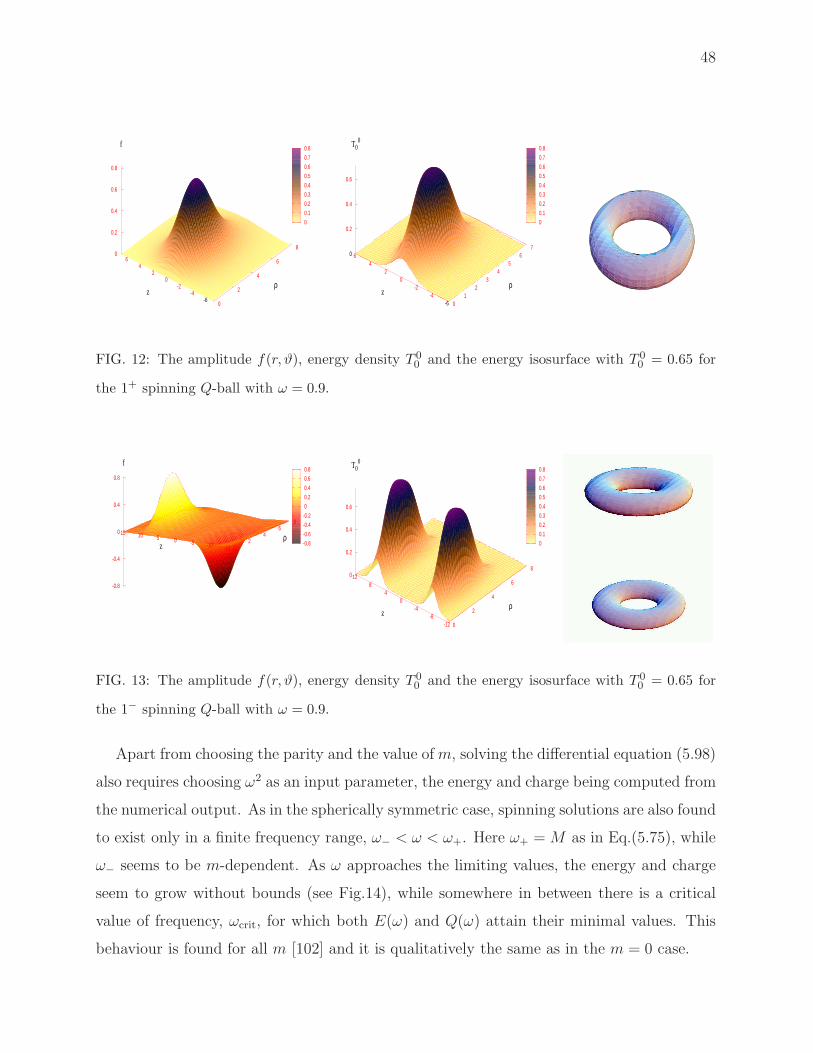
48
0
0.1
0.2
0.3
0.4
0.5
0.6
0.7
0.8
0
2
4
6
8
ρ-6
-4-2
0 2
4 6
z
0
0.2
0.4
0.6
0.8
f
0
0.1
0.2
0.3
0.4
0.5
0.6
0.7
0.8
0 1
2 3
4 5
6 7
ρ
-6-4
-2 0
2 4
6
z
0
0.2
0.4
0.6
T00
FIG. 12: The amplitude f(r, ϑ), energy density T 00 and the energy isosurface with T 0
0 = 0.65 for
the 1+ spinning Q-ball with ω = 0.9.
-0.8
-0.6
-0.4
-0.2
0
0.2
0.4
0.6
0.8
0 2
4 6
8
ρ-15-10-5 0 5 10 15
z
-0.8
-0.4
0
0.4
0.8
f
0
0.1
0.2
0.3
0.4
0.5
0.6
0.7
0.8
0
2
4
6
8
ρ
-12-8
-4 0
4 8
12
z
0
0.2
0.4
0.6
T00
FIG. 13: The amplitude f(r, ϑ), energy density T 00 and the energy isosurface with T 0
0 = 0.65 for
the 1− spinning Q-ball with ω = 0.9.
Apart from choosing the parity and the value ofm, solving the differential equation (5.98)
also requires choosing ω2 as an input parameter, the energy and charge being computed from
the numerical output. As in the spherically symmetric case, spinning solutions are also found
to exist only in a finite frequency range, ω− < ω < ω+. Here ω+ = M as in Eq.(5.75), while
ω− seems to be m-dependent. As ω approaches the limiting values, the energy and charge
seem to grow without bounds (see Fig.14), while somewhere in between there is a critical
value of frequency, ωcrit, for which both E(ω) and Q(ω) attain their minimal values. This
behaviour is found for all m [102] and it is qualitatively the same as in the m = 0 case.

49
The existence of a minimal value of the Q-ball charge implies that the angular momentum
(5.100) cannot be arbitrarily small. Q-balls cannot therefore rotate slowly. They show a
discrete spectrum of spinning excitations.
Although it is difficult to qualitatively analyse the behaviour of the m 6= 0 solutions,
there are some analogies with the m = 0 case. Specifically, Q-balls become large as ω → ω±.
For ω → ω− they can be viewed as squashed spheroids, homogeneously filled inside, which
reminds of the thin wall approximation. Unfortunately, an analog of the step function
solution (5.95) does not directly apply for m 6= 0, since the function f cannot be constant
inside the ball because it must vanish at the symmetry axis. Instead, f increases as one moves
away from the axis and reaches maximal values at the surface of the spheroids, after which
it rapidly goes to zero. The energy density is approximately constant inside the spheroid,
with a slight increase at its surface, and rapidly vanishes outside it. For ω → ω+ solutions
also become large spheroids, but this time they are hollow, with the maximal energy density
concentrated at the surface and being close to zero everywhere else. It seems that the thick
wall approximation (5.96) can be directly generalized to the axially symmetric case to give
f(r, θ) ≈√
2Mω y(Mωr, θ) where Mω → 0 and y(r, θ) fulfills (∆− m2
r2 sin2 θ+ y2 − 1)y = 0.
If one considers Q and not ω as the solution parameter then, using E(ω) and Q(ω) to
express E in terms of Q, one discovers that the function E(Q) is double-valued with a cusp,
as shown in Fig.14 [102]. For a given Q there are thus two different spinning Q-ball solutions
with different energies. Solutions from the less energetic branch correspond to the ω < ωcrit
parts of the E(ω), Q(ω) curves in Fig.14. As in the m = 0 case, the plots shown in Fig.14
demonstrate for large Q the linear dependence, E = ω±Q. This can again be explained by
the general relation (5.91), implying that for large Q one can neglect the gradient energy E2
as compared to Q.
The existence of two different solutions with the same Q suggests that the more energetic
of them is unstable. In fact, it follows from Eq.(5.91) that the energy-to-charge ratio for
Q-balls is E/Q = ω + 2E2/3Q. For the upper branch solutions one has ω → ω+ = M for
large Q, implying that E/Q = M + O(Q−2) where the subleading term can in principle
be positive or negative, depending on the details of the Q-ball potential. In the present
case it is positive, as can be seen in Fig.14, so that the upper branch Q-balls are unstable
with respect to decay into free particles. The same argument for the lower branch solutions
gives E/Q = ω− < M for large Q, so that they cannot decay into free particles. However,

50
0
200
400
600
800
0.5 0.6 0.7 0.8 0.9 1 1.1
ω
Q
E
m=1, λ=1, a=2, b=1.1 200
300
400
500
600
100 200 300 400 500 600 700 800
E
Q
λ=1, a=2, b=1.1
m=1
E=MQ
0.9
1
1.1
200 300 400 500 600
E/(QM)
FIG. 14: Energy and charge E(ω), Q(ω) (left) and E(Q) (right) for the 1+ spinning Q-balls. For
large Q one has E(Q) = ω−Q and E(Q) = ω+Q for the lower an upper branch, respectively. The
upper branch solutions are unstable, since E/(MQ) > 1, while the lower branch solutions are
stable for large enough Q.
there can be other decay modes, and so the stability analysis is needed. In fact, the m = 0
lower branch Q-balls are known to be stable [44]. The stability analysis of the even parity
solutions with m 6= 0 will be described below in Sec.VIIB. It seems that for |m| = 1 the
lower branch solutions are stable only for large enough Q, while already for |m| = 2 all of
them are unstable – they seem to decay by splitting into several non-spinning Q-balls.
It is plausible that spinning generalizations could also be constructed for the excited
spherically symmetric Q-balls with n > 0. The complete family of spinning Q-balls should
therefore contain not only m± solutions, but also the excited (n,m±) solutions with n =
1, 2, . . . for which the amplitude f(r, ϑ) exhibits nodes. More precisely, parametrizing the
(ρ, z) plane by a complex variable w = ρ + iz, one can expect the amplitude f(w) of
the (n,m+) and (n,m−) solutions to have the same zeros as, respectively, ℜ(F+n (w)) and
ℑ(F−n (w)), where
F±n (w) =
n∏
j=1
α±j (w − ρ±j ), (5.102)
with some suitably chosen α±j ∈ C and ρ±j > 0. However, very little is known about such
excited solutions at present.

51
3. Twisted Q-balls
Here and in the next subsection we briefly describe our new results on further general-
izations of the spinning Q-balls, not yet discussed in the literature. Let us consider again
the theory (5.72), but generalize the field ansatz to include an independent phase,
Φ = ei(ωt+mϕ−nψ(r,θ))f(r, θ) ≡ (X(r, ϑ) + iY (r, ϑ))ei(ωt+mϕ). (5.103)
We require the phase function ψ(r, ϑ) to increase by 2π after one revolution around the
contour C shown in Fig.2. The overall phase ωt + mϕ − nψ(r, θ) then winds around the
circle S and along the contour C, exactly as for the Faddeev-Hopf field Eq.(2.10). For regular
fields f(r, ϑ) vanishes at C and has n zeros inside C. The solutions are thus characterized by
two integers (n,m) giving rise to the ‘topological charge’ N = nm, although now this does
not represent a genuine topological invariant. We shall call Q-balls with N 6= 0 twisted,
by analogy with twisted loops in the Faddeev-Hopf theory, while those with N = n = 0
described above will be called simply spinning or ‘non-twisted’.
-0.8-0.6-0.4-0.2 0 0.2 0.4 0.6 0.8 1
0 4
8 12
ρ-8
0 8
z
-0.75
-0.5
-0.25
0
0.25
0.5
0.75
1
X
-0.8
-0.6
-0.4
-0.2
0
0.2
0.4
0.6
0.8
0 3
6 9
ρ-16-8 0 8 16
z
-0.75
-0.5
-0.25
0
0.25
0.5
0.75
Y
FIG. 15: Profiles of the (1, 1) twisted Q-ball with ω = 0.9.
The field equations read
(
∆− m2
r2 sin2 ϑ+ ω2
)
X =1
2
∂U(√X2 + Y 2)
∂X,
(
∆− m2
r2 sin2 ϑ+ ω2
)
Y =1
2
∂U(√X2 + Y 2)
∂Y, (5.104)
where one can require X, Y to be symmetric and antisymmetric, respectively, with respect to

52
reflections in the equatorial plane. The simplest twisted solutions are obtained for n = m = 1
and are shown in Fig.15.
3
6
9
12
15
ρ
-15-10
-5 0
5 10
15 20
z
0
0.25
0.5
0.75
1
T00
FIG. 16: Energy density for the (1, 1) twisted Q-ball with ω = 0.9 (left) and the isosurfaces of
constant energy density with T 00 = 0.3 (right).
The profiles of the energy density look spectacular; see Fig.16. It is unclear at present
whether these solutions are dynamically stable, but they certainly exist as solutions of the
elliptic system (5.104). The twisted Q-balls are much more heavy than the non-twisted ones.
For example, for ω = 0.9 we found for the twisted (1, 1) solution the energy E = 929.34, while
the non-twisted 1+ and 1− spinning Q-balls have, respectively, E = 169.27 and E = 338.66.
4. Spinning gauged Q-balls
Another possibility to generalize the spinning Q-balls is to couple them to a gauge field
within the theory
LgQ[Aµ,Φ] = −1
4FµνF
µν + LQ[Φ]. (5.105)
Here Fµν = ∂µAν − ∂νAµ while LQ[Φ] is the same Q-ball Lagrangian as in (5.72) but with
the derivatives of Φ replaced by the covariant derivatives, ∂µΦ → DµΦ = (∂µ − igAµ)Φ
where g is the gauge coupling constant. This theory is in fact the U(1) version of the general
gauge field model (3.50). The local gauge transformations (3.52) now read Φ → Φeigα,

53
Aµ → Aµ + ∂µα while the field equations (3.53) assume the form
∂µFµν = ig (DµΦ)∗Φ− Φ∗(DµΦ) ≡ gjν ,
DµDµΦ = − ∂U
∂|Φ|2 Φ. (5.106)
The conserved Noether charge analogues to the Q-ball charge Eq.(5.77) is
Q =
∫
j0 d3x =
1
g
∮
~Ed~S ≡ 4πQel
g, (5.107)
where Qel is the electric charge. Spherically symmetric solutions of this model were discussed
in Ref.[115].
We make the ansatz
Aµdxµ = A0(r, ϑ)dt+ Aϕ(r, ϑ) sin θdϕ, Φ = f(r, ϑ)ei(mϕ+ωt), (5.108)
with real f(r, ϑ), and require the gauge field to vanish at infinity, while at the z-axis Aϕ =
∂θA0 = 0. Although Φ depends on t, ϕ, this dependence can be gauged away, so that the
system is manifestly stationary and manifestly axially symmetric. Numerically solving the
field equations gives spinning Q-balls with a long range gauge field which behaves for large
r as (m being the magnetic dipole moment)
A0 =Qel
r+ . . . , Aϕ =
m sin θ
r2+ . . . . (5.109)
In the limit g → 0 they reduce to the non-gauged spinning Q-balls. It seems that solutions
exist if only g does not exceed a certain maximal value gmax(ω) (see Fig.17). This feature
can be understood qualitatively [115]: since Q-balls can be viewed as condensate states of
mutually attracting scalar particles, gauging them creates an electric repulsion that destroys
the condensate for large enough g.
Since the symmetries of the solutions are manifest, one can use the surface integral
formula (4.66) for the angular momentum. Applying the symmetry equations (4.64) to the
ansatz (5.108) gives Wϕ = m/g, inserting which to (4.66) and using (5.109) yields
J =
∮(
m
g− Aϕ
)
~E ~dS =4πQelm
g= Qm. (5.110)
This shows that spinning is possible in manifestly stationary and manifestly axially sym-
metric systems where all the spinning phases can be gauged away.

54
0.9
0.95
1
1.05
1.1
160 180 200 220 240
E/(
QM
)
Q
g=0
g=0.055
g=0.13
g=0.22 150
200
250
300
0.75 0.8 0.85 0.9 0.95 1 1.05 1.1
ω
E(ω)
200
400
600
800
1000
0 0.05 0.1 0.15 0.2 0.25
E
g
ω=1
ω=0.77
ω=0.67
180
190
200
0 0.05 0.1 0.15 0.2
ω=1
FIG. 17: Left: the energy E(ω) and E(Q)/(QM) for several values of g for the 1+ gauged Q-balls.
Right: the energy E(g) for several values of ω for the 1+ solutions. The plots of Q(ω) and Q(g)
look qualitatively similar.
As seen in Fig.17, the dependence of solutions on ω is similar to that in the ungauged
case: they exist for a limited range of ω. Expressing E in terms of Q gives again a two-
branch function E(Q), the solutions from the lower branch being stable for large enough Q
with respect to decay into free particles. E,Q cannot be arbitrarily large for g 6= 0, since the
electric and scalar field contributions to the energy grow as Q2el ∼ Q2 and Q, respectively,
and so for large Q the electric term dominates and destroys the soliton.
For small g solutions can be represented as Φ = Φ(0) + g2Φ(2) + . . . and Aµ = gA(1)µ + . . .
where Φ(0) is the non-gauged Q-ball. The energy is E(g) = E(0)+g2E(2)+. . . and calculating
E(2) reveals that it is not sign definite – due to the electric field contribution. The plots in
Fig.17 show that it can be both positive and negative, depending on the solution.
5. Spinning interacting Q-balls
Yet another way to generalize Q-balls is to couple to each other several copies of the the-
ory. This allows one to consider ‘non-linear superpositions’ of individual Q-balls. Although
this idea has already been considered in the literature [30], we have reconsidered it and
found some curious solutions which could be interesting in the context of our discussion. In
the simplest case one can choose
L[Φ1,Φ2] = LQ(Φ1) + LQ(Φ2)− γ|Φ1|2|Φ2|2, (5.111)

55
FIG. 18: Energy isosurfaces with T 00 = 0.1 for the m1 = 0, m2 = 3 ‘Saturn’ (left) and with
T 00 = 0.3 for the m1 = 1, m2 = 3 bi-ring (right) solutions in the theory (5.111).
where LQ(Φ1) and LQ(Φ2) are two copies of the Q-ball Lagrangian (5.72). Setting
Φ1 = ei(ω1t+m1ϕ)f1(r, θ), Φ2 = ei(ω2t+m2ϕ)f2(r, θ), (5.112)
it is interesting to consider solutions with m1 6= m2. Choosing ω1 = ω2 = 1, γ = 1 and
0 0.05 0.1 0.15 0.2 0.25 0.3 0.35 0.4 0.45
0 2 4 6 8 10 12 14 16
ρ
-10
-5
0
5
10
z
0
0.2
0.4
T00
FIG. 19: The energy density T 00 and the T 0
0 = 0.1 energy isosurface for the m1 = 0, m2 = 3 ‘hoop’
solution in the theory (5.111).
restricting to the even parity sector, we find solutions of the ‘Saturn type’, with a central
concentration of the energy density produced by the first scalar with m1 = 0 and surrounded
by a ring created by the second scalar with m2 > 0 (Fig.18), solutions for m2 > m1 > 0 with
bi-ring profiles (Fig.18), as well as solutions describing a superposition of a straight ‘Q-ball
vortex’ with m1 = 0 ‘hooped’ by a Q-ball ring with m2 > 0 (Fig.19).
B. Skyrmions
The first known example of topological solitons in 3+1 dimensions was suggested almost
50 years ago within the non-linear relativistic field theory model proposed by T.H.R. Skyrme

56
[157]. These solitons are now called skyrmions. Skyrme himself considered them as field
theoretic realizations of baryons. Nowadays the Skyrme model is regarded as an effective,
low energy approximation of QCD [5],[4]. In this approximation the static skyrmions are
promoted to spinning objects by making use of the effective rigid body approximation that
will be considered below. The masses of the spinning skyrmions obtained in this way are
then compared to the hadron masses.
The question of whether spinning skyrmions really exist as stationary field theory objects
was addressed only very recently in Ref.[18], whose authors constructed spinning skyrmions
by applying the same mechanism as for the Q-balls and arrived at conclusions which differ
considerably from those obtained within the rigid body approximation.
Since there exist excellent descriptions of the Skyrme model and its solutions in the
literature [120],[121], we shall very briefly summarize only the features essential for our
discussion. The fundamental field variables in the theory comprise an SU(2)-valued matrix
U(xµ) which satisfies field equations for the Lagrangian
LS[U ] = tr
(
1
2∂µU
†∂µU +1
8[∂µU
†, ∂νU ][∂µU †, ∂νU ]
)
. (5.113)
It is convenient to introduce a pure gauge SU(2) connection,
Aµ = iU †∂µU ≡ τaAaµ, ∂µAν − ∂νAµ = i[Aµ,Aν ], (5.114)
in terms of which the field equations read
∂µ(
Aµ −1
4[[Aµ,Aν ],A
ν ]
)
= 0. (5.115)
The energy for static fields is
E[U ] =
∫
tr
(
1
2(Ak)
2 − 1
8([Ai,Ak])
2
)
d3x . (5.116)
For the energy to be finite the field U(x) should approach a constant value at infinity, which
can be chosen to be the unit matrix, so that lim|x|→∞U(x) = 1. This allows one to replace
R3 by its one-point compactification S3. Since SU(2) is topologically also S3 it follows that
any finite energy field configuration can be viewed as a map, U(x) : S3 → S3, and can
therefore be characterized by the integer degree of map,
N [U ] =i
24π2
∫
tr (ǫijkAiAjAk) d3x . (5.117)

57
This topological charge is called in Skyrme theory ‘baryon number’. Fixing it the energy
obeys the Bogomol’nyi type inequality
E[U ] ≥ 12√
2π2|N [U ]|, (5.118)
which can be easily obtained by rearranging terms in the integrand in (5.116). The existence
of this lower bound suggests looking for energy minimizers in each topological sector.
It will be convenient for what follows to parametrize the matrix U in terms of two complex
scalar fields φ, σ subject to the normalization condition |φ|2 + |σ|2 = 1 as
U =
φ iσ∗
iσ φ∗
. (5.119)
Simplest skyrmions are spherically symmetric, U = exp(iχ(r)x · τ/r), hence
φ = cosχ(r) + i sinχ(r) cosϑ, σ = sinχ(r) sinϑeiϕ. (5.120)
Inserting this to Eqs.(5.115) the variables separate and the equations reduce to an ODE
for χ(r). This equation admits globally regular solutions with the boundary conditions
χ(0) = Nπ and χ(∞) = 0 for any value of the topological charge N . However, it seems that
only for N = ±1 these solutions correspond to the absolute energy minimum, while those
for |N | > 1 are local minima or saddle points. Global energy minima for |N | > 1 are not
spherically symmetric and can be obtained by directly minimizing the energy (5.116). For
|N | = 2 they are axially symmetric, with the constant baryon number isosurfaces having
toroidal shape, so they are somewhat similar to knots. However, higher charge skyrmions
do not resemble knots at all and look like polyhedral shells. Their detailed description can
be found in the monograph [121].
1. Skyrme versus Faddeev-Skyrme
It is worth emphasizing the similarity between the Skyrme and Faddeev-Skyrme models.
Both can be represented in the form (up to normalization)
L[φ] = ∂µφ · ∂µφ−1
4(∂µφ · ∂µφ)2 +
1
4(∂µφ · ∂νφ)(∂µφ · ∂νφ) (5.121)
where φ is a vector normalized by the condition φ · φ = 1. In the Faddeev-Skyrme case
one has φ = φa with a = 1, 2, 3 so that the target space is S2. In the Skyrme model

58
one has φ = (φ0, φa) with a = 1, 2, 3 so that the target space is S3, the Skyrme field being
U = φ0+iφaτa. One can also construct a generalized theory whose target space ‘interpolates’
between S2 and S3 and so it includes both models as special cases [175].
The Faddeev-Skyrme model can be regarded as a consistent truncation of the Skyrme
theory. Specifically, if n = na is a solution of the Faddeev-Skyrme model, then φ = (0, na)
solves the equations of the Skyrme model. As a result, knot solitons can be embedded into
the Skyrme model [123], [37], although their stability properties will then be different.
Another embedding of knot solitons into Skyrme theory is obtained by expressing the
fields Aµ and n in terms of the CP 1 coordinates φ, σ using Eqs.(2.28),(2.30),(2.31). The
Skyrme field U is then given by Eq.(5.119). Although this correspondence does not map
solutions to solutions, the advantage now is that the baryon number N [U ] is exactly equal
to the Hopf charge N [n]. This follows from the fact that A3µ = −Aµ and Fµν = 2(A1
µA2ν −
A1νA
2µ) due to Eq.(5.114). With this, the expression (5.117) for the baryon number exactly
reduces to the expression (2.9) for the Hopf charge. For example, using the parametrization
(2.32) for the CP 1 scalars φ, σ with the Hopf charge N [n] = nm gives with (5.119) the
Skyrme field U with N [U ] = nm.
The Hopf charge N [n] will determine in this case also the winding number of the pure
gauge field Ak = iU †∂kU . If n is an energy minimizer then the pure gauge Ak is maximally
abelian [164].
The correspondence can also be used in the opposite direction to construct n with a
given Hopf charge out of U with a given baryon number. If U is spherically symmetric,
then n is axially symmetric, as can be seen comparing Eq.(5.120) and Eq.(2.16). Using
approximations for U gives in this way approximate solutions for n [173].
2. Spinning skyrmions
Let us consider the N = 1 static, spherically symmetric skyrmion described by Eq.(5.120).
Its spinning analog in the rigid body approximation is obtained by simply replacing in
Eq.(5.120)
ϕ→ ϕ+ ωt , (5.122)
which gives a non-zero value to the angular momentum. It is in fact precisely this type of
approximation that is often implicitly assumed in the literature when talking about spinning

59
solitons. In this approximation spinning solitons do not change their shape and the radiation
effects are neglected, which are natural assumptions if the rotation is slow. However, if ω is
not small, then this description does not approximate the true spinning solutions any more
but simply gives field configurations with J 6= 0. If one uses them as initial data, then their
temporal evolutions will be certainly accompanied by radiation carrying J away, and it is
not clear if the system will finally relax to a state with J 6= 0.
In order to construct truly spinning skyrmions with N = 1, Battye, Krusch and Sut-
cliffe (BKS) [18] generalize the spherically symmetric ansatz (5.119),(5.120) to the axially
symmetric, non-manifestly stationary one, which can be parametrized as
φ = cosΘ
2eiψ, σ = sin
Θ
2ei(ϕ+ωt). (5.123)
It is instructive to compare this with the ansatz (2.32) for the axially symmetric hopfions
with m = n = 1. They also add to the Lagrangian (5.113) the mass term
M2 tr(U − 1). (5.124)
Instead of solving the field equations for Θ(r, ϑ), ψ(r, ϑ) they minimize the energy with fixed
J , whose expression is similar to the one in Eq.(5.101). The frequency ω for their solutions
is a parameter in the interval
0 ≤ ω2 < M2, (5.125)
both the energy and angular momentum increasing with ω. The latter feature is very
interesting – for spinning skyrmions J is a continuous parameter that can be arbitrarily
small, so that they can rotate slowly. To compare, Q-balls cannot rotate slowly. Although
BKS do not emphasize this, it seems that both E and J should blow up as ω2 → M2 since
the fields localized by the factor exp(−√M2 − ω2 r) become then long range.
Trying to adjust M2 and the energy scale to reproduce the pion and hadron masses and
their spins, BKS discover that this requires moving to the parameter region where deviations
of spinning skyrmions from spherical symmetry are large. They conclude that the rigid body
approximation does not provide an adequate description of spinning skyrmions.
The results of BKS have been confirmed by solving the field equations by Ioannidou,
Kleihaus and Kunz [94] (who studied in fact gravity-coupled skyrmions, but considered the
Minkowski space limit as well).
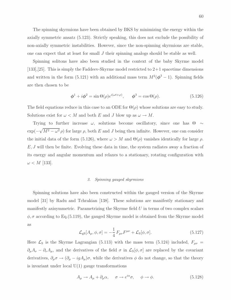
60
The spinning skyrmions have been obtained by BKS by minimizing the energy within the
axially symmetric ansatz (5.123). Strictly speaking, this does not exclude the possibility of
non-axially symmetric instabilities. However, since the non-spinning skyrmions are stable,
one can expect that at least for small J their spinning analogs should be stable as well.
Spinning solitons have also been studied in the context of the baby Skyrme model
[133],[25]. This is simply the Faddeev-Skyrme model restricted to 2+1 spacetime dimensions
and written in the form (5.121) with an additional mass term M2(φ3 − 1). Spinning fields
are then chosen to be
φ1 + iφ2 = sin Θ(ρ)ei(ωt+ϕ), φ3 = cos Θ(ρ). (5.126)
The field equations reduce in this case to an ODE for Θ(ρ) whose solutions are easy to study.
Solutions exist for ω < M and both E and J blow up as ω →M .
Trying to further increase ω, solutions become oscillatory, since one has Θ ∼exp(−
√M2 − ω2 ρ) for large ρ, both E and J being then infinite. However, one can consider
the initial data of the form (5.126), where ω > M and Θ(ρ) vanishes identically for large ρ.
E, J will then be finite. Evolving these data in time, the system radiates away a fraction of
its energy and angular momentum and relaxes to a stationary, rotating configuration with
ω < M [133].
3. Spinning gauged skyrmions
Spinning solutions have also been constructed within the gauged version of the Skyrme
model [31] by Radu and Tchrakian [138]. These solutions are manifestly stationary and
manifestly axisymmetric. Parametrizing the Skyrme field U in terms of two complex scalars
φ, σ according to Eq.(5.119), the gauged Skyrme model is obtained from the Skyrme model
as
LgS[Aµ, φ, σ] = −1
4FµνF
µν + LS[φ, σ]. (5.127)
Here LS is the Skyrme Lagrangian (5.113) with the mass term (5.124) included, Fµν =
∂µAν − ∂νAµ, and the derivatives of the field σ in LS[φ, σ] are replaced by the covariant
derivatives, ∂µσ → (∂µ − igAµ)σ, while the derivatives φ do not change, so that the theory
is invariant under local U(1) gauge transformations
Aµ → Aµ + ∂µα, σ → eiασ, φ→ φ. (5.128)

61
Radu and Tchrakian [138] generalize the ansatz (5.123) as
Aµdxµ = A0dt+ Aϕ sinϑ dϕ, φ = cos
Θ
2eiψ, σ = sin
Θ
2ei(mϕ+ωt), (5.129)
where A0, Aϕ,Θ, ψ depend on r, ϑ. This ansatz is manifestly stationary and manifestly
axially symmetric, since its t, ϕ-dependence can be removed by a gauge transformation.
The topological charge (5.117) is N = m. Integrating the field equations gives globally
regular solutions with finite energy and a longrange gauge field, which is at large r
A0 =Qel
r+ . . . , Aϕ =
m
r2sinϑ+ . . . , (5.130)
where Qel,m are the electric charge and dipole moment. This feature is similar to that for
the gauged Q-balls in Eq.(5.109). The angular momentum can be calculated in the same
way as in Eq.(5.110), with a similar result,
J =4πQelm
g. (5.131)
However, unlike for Q-balls, J can be arbitrarily small if ω is small. The dependence of
solutions on ω is qualitatively similar to that for the global skyrmions: they exist only for
a finite frequency range, both E and J growing with ω. For ω = 0 the solutions reduce to
the non-spinning gauged skyrmions found in Ref.[134].
The stability of spinning gauged skyrmions has not been studied. They probably have
less chance to be stable than their global counterparts – since gauging introduces additional
degrees of freedom that can produce instabilities.
C. Rotating monopole-antimonopole pairs
There are other known solutions with non-zero angular momentum. They are mani-
festly stationary and manifestly axisymmetric, but they describe rotations in multisoliton
systems and not spinning of a single soliton. Let us consider the already mentioned above
monopole-antimonopole solutions in the Yang-Mills-Higgs theory (3.50). Their existence was
demonstrated by Taubes [161] and they were explicitly constructed by Kleihaus and Kunz
[100] within the ansatz (3.55) with k = 2, m = 1. These solutions are static, purely mag-
netic and manifestly axisymmetric (since their ϕ-dependence can be gauged away) and with
vanishing magnetic charge. The Higgs field Φ shows two simple zeros at two spatial points

62
separated by a finite distance (see Fig.20). These two points correspond to the positions of
the monopole and antimonopole. The analysis of the charge and current distributions similar
to that described in Sec.III B shows that the system also contains a circular electric current,
as shown in Fig.20. The magnetic field created by this current acts against the Coulom-
bian attraction between the monopole and antimonopole, which presumably stabilizes the
system.
0 0.1 0.2 0.3 0.4 0.5 0.6 0.7 0.8 0.9
0
3
6
9
ρ
-10
-5
0
5
10
z
0.25
0.5
0.75
|φ| +P
−P
j
Bj
BP
FIG. 20: Left: the Higgs field amplitude for the monopole-antimonopole solution in the limit where
the Higgs field potential vanishes. It is shown only for a limited region around the origin, while at
infinity it approaches the unit value. Right: the charge and current distributions for this solution
exhibits essentially the same structure as for the monopole rings, shown in Fig.8.
Since there is no electric field for these solutions, their angular momentum (4.66) is zero.
However, in the limit where the Higgs potential vanishes, the Lagrangian (3.50) admits the
global symmetry [27],[40]
A0 → A0 cosh γ + Φ sinh γ, Φ→ Φ cosh γ + A0 sinh γ, Ak → Ak, (5.132)
and this allows one to produce solutions with an electric field starting from purely magnetic
solutions. As was noticed in [88], this transformation may also generate a non-zero angular
momentum
J ∼ sinh γ, (5.133)
provided that the original purely magnetic solution is not spherically symmetric and does not
satisfy the first order Bogomol’nyi equations [27]. The latter condition excludes from consid-
eration the (multi)monopole solutions of these equations. However, applying the symmetry
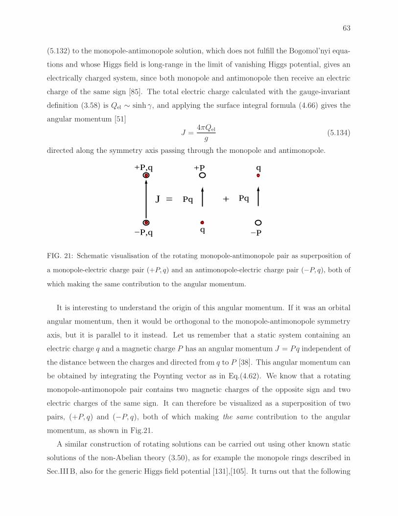
63
(5.132) to the monopole-antimonopole solution, which does not fulfill the Bogomol’nyi equa-
tions and whose Higgs field is long-range in the limit of vanishing Higgs potential, gives an
electrically charged system, since both monopole and antimonopole then receive an electric
charge of the same sign [85]. The total electric charge calculated with the gauge-invariant
definition (3.58) is Qel ∼ sinh γ, and applying the surface integral formula (4.66) gives the
angular momentum [51]
J =4πQel
g(5.134)
directed along the symmetry axis passing through the monopole and antimonopole.
J = +
+P,q
−P,q
+P
q
q
−P
Pq Pq
FIG. 21: Schematic visualisation of the rotating monopole-antimonopole pair as superposition of
a monopole-electric charge pair (+P, q) and an antimonopole-electric charge pair (−P, q), both of
which making the same contribution to the angular momentum.
It is interesting to understand the origin of this angular momentum. If it was an orbital
angular momentum, then it would be orthogonal to the monopole-antimonopole symmetry
axis, but it is parallel to it instead. Let us remember that a static system containing an
electric charge q and a magnetic charge P has an angular momentum J = Pq independent of
the distance between the charges and directed from q to P [38]. This angular momentum can
be obtained by integrating the Poynting vector as in Eq.(4.62). We know that a rotating
monopole-antimonopole pair contains two magnetic charges of the opposite sign and two
electric charges of the same sign. It can therefore be visualized as a superposition of two
pairs, (+P, q) and (−P, q), both of which making the same contribution to the angular
momentum, as shown in Fig.21.
A similar construction of rotating solutions can be carried out using other known static
solutions of the non-Abelian theory (3.50), as for example the monopole rings described in
Sec.III B, also for the generic Higgs field potential [131],[105]. It turns out that the following

64
general relation holds
J =2πmQel
g[1 + (−1)k] (5.135)
where m, k are the winding numbers in the ansatz (3.56) [131], [51], [105]. Therefore,
using Eq.(3.59), the angular momentum is zero in the presence of a nonvanishing magnetic
charge, even though T 0ϕ 6= 0 [105], while the relation (5.131) is still valid for solutions with
zero magnetic charge.
Since they are related to the monopole-antimonopole solution known to be unstable
[161], rotating monopole-antimonopole pairs are very probably unstable as well. However,
the mechanism of their rotation is interesting and suggests, in particular, a possibility to
have stationary, non-radiating spinning solitons without axial symmetry.
Specifically, in theories without radiation, as in classical mechanics, steadily rotating
bodies can be totally asymmetric. However, if they carry an electric charge distribution,
say, then their electric dipole momentum will depend on time, hence producing radiation,
unless they are axially symmetric. This suggests that non-radiating spinning field systems
should be axially symmetric – the assumption usually made when studying spinning solitons.
An interesting illustration of this has been found by Hen and Karliner [87], who analyze
situations where rapidly spinning systems can loose axial symmetry. A classical example
of this phenomenon is provided by the rotating Jacobi ellipsoids in Newtonian gravity – a
theory without radiation. Hen and Karliner study spinning baby skyrmions on a compact
(sphere or disk) 2D space, in which case there is no radiation, and find that the system
looses axial symmetry for large enough J . However, as was discussed above, in the limit of
infinite R2, when radiation can exist, spinning baby skyrmions remain axially symmetric for
any value of J [133] – since otherwise they would radiate.
Now, the rotating monopole-antimonopole pairs suggest a possibility to have non-
radiating, non-axially symmetric rotation even in theories with radiation. This can be
achieved by simply taking three or more dyons not aligned along one direction. Of course,
this should be realized by constructing a smooth, static, non-axially symmetric, finite energy
solutions in a non-Abelian gauge field theory. If they exist, they may have a non-zero J due
to the same mechanism as for the rotating monopole-antimonopole pairs.

65
VI. VORTONS
We are now ready to explicitly construct vortons as localized, finite energy solutions of
the elliptic field equations. By construction, they are stationary and non-radiating. Our
results can be viewed as complementary to those obtained by Battye, Cooper and Sutcliffe
[17] (although in a completely different context) and by Lemperier and Shellard [118].
A. The Witten model
Vortons were originally suggested [46], [48], [45], [47] in the context of Witten’s model
of superconducting cosmic strings [177]. This model contains two Abelian vectors A(a)µ
(a = 1, 2) interacting with two complex scalars φ and σ with the Lagrangian density
LW = −1
4
∑
a=1,2
F (a)µν F
(a)µν +Dµφ∗Dµφ+Dµσ
∗Dµσ − U. (6.136)
Here F(a)µν = ∂µA
(a)ν − ∂νA(a)
µ are the Abelian field strengths, the gauge covariant derivatives
of the scalars are Dµφ = (∂µ− ig1A(1)µ )φ and Dµσ = (∂µ− ig2A
(2)µ )σ where g1 and g2 are the
gauge coupling constants. The scalar field potential is
U =1
4λφ(|φ|2 − η2
φ)2 +
1
4λσ|σ|2(|σ|2 − 2η2
σ) + γ|φ|2|σ|2, (6.137)
where λφ, λσ , ηφ, ησ and γ are positive constants. This theory is invariant under local
U(1)×U(1) gauge transformations, so that there are two conserved Noether currents.
The theory admits stationary, cylindrically symmetric solutions of the vortex type, sup-
porting a constant non-zero value of one of the Noether currents [177], [13], [86], [91], [46],
[7], [132]. These are the superconducting cosmic strings. Vortons are supposed to be loops
made of these strings.
Within the full gauged model (6.136) explicit vorton constructions have never been at-
tempted – due to the complexity of the problem. However, the problem simplifies in the
global limit of this model, for g1 = g2 = 0. The gauge fields then decouple and the theory
reduces to
L = ∂µφ∗∂µφ+ ∂µσ
∗∂µσ − U (6.138)
so that the U(1)×U(1) internal symmetry becomes global. This global theory still keeps some
essential features of the original local model. In particular, it still admits superconducting
66
vortex solutions, even though the corresponding current is now global and not local. One
can therefore study global vortons made of these vortices, which was in fact the subject
of Refs.[17],[118]. Below we shall construct the global vortons as stationary solutions of
the field equations in the model (6.138), which has not been done before. The question of
whether these solutions can be generalized within the full gauged model (6.136) remains
open.
One can absorb ηφ in the definition of φ, σ in (6.138) to achieve ηφ = 1. Since the overall
normalization of the potential could be changed by rescaling the spacetime coordinates,
xµ → Λxµ, one can impose one more condition on the remaining four parameters λφ, λσ, ησ, γ,
although we do not use this option.
A minimal value of the potential is achieved for |φ| = ηφ = 1 and |σ| = 0, in which
case U = 0. This minimum is global if 4γ2 > λσλφ. The perturbative spectrum of field
excitations around this vacuum consists of two massless Goldstone particles, corresponding
to excitations of the phases of the fields, and of two Higgs bosons with the masses
Mφ =√
λφ, Mσ =
√
γ − 1
2λση2
σ. (6.139)
The global U(1)×U(1) symmetry of the theory, φ → φeiα1 , σ → σeiα2 , leads to the
conserved currents
jµ(φ) = 2ℜ(iφ∗∂µφ), jµ(σ) = 2ℜ(iσ∗∂µσ), (6.140)
with ∂µJµ(φ) = ∂µJ
µ(σ) = 0. The energy-momentum tensor is
Tµν = ∂µφ∗∂νφ+ ∂νφ
∗∂µφ+ ∂µσ∗∂νσ + ∂νσ
∗∂µσ − gµνL , (6.141)
where gµν is the spacetime metric.
The Lagrangian field equations in the theory (6.138) read
∂µ∂µφ+
∂U
∂|φ|2 φ = 0, ∂µ∂µσ +
∂U
∂|σ|2 σ = 0. (6.142)
Expressing the complex scalar fields in terms of their amplitudes and phases as
φ = f1 eiψ1 , σ = f2 e
iψ2 , (6.143)
equations (6.142) assume the form (a = 1, 2)
∂µ∂µfa = (∂µψa∂
µψ2)fa −1
2
∂U
∂fa, ∂µ(f
2a∂
µψa) = 0. (6.144)
67
These equations admit cylindrically symmetric vortex solutions discussed by several authors
(see e.g. [46], [118], [84]). For these solutions one has
φ = f1(ρ)einϕ, σ = f2(ρ)e
i(pz+ωt) , (6.145)
where n ∈ Z and p, ω ∈ R, with 0 ← f1(ρ) → 1 and f2(0) ← f2(ρ) → 0 as 0 ← ρ → ∞,
respectively. The field φ thus vanishes in the vortex core and approaches the finite vacuum
value at infinity, while σ develops a non-zero condensate value in the core and vanishes
at infinity. The fields φ, σ are sometimes referred to as vortex field and condensate field,
respectively. The phase of φ changes by 2πn after one revolution around the vortex, while
the phase of σ increases along the vortex. The z-dependence of the condensate field gives
rise to a non-zero momentum along the vortex, P =∫
T 0z d
3x ∼ p.
The qualitative vorton construction usually discussed in the literature suggests taking a
piece of length L of the vortex and identifying its extremities to form a loop. The momentum
along the vortex will then circulate along the loop, thus becoming an angular momentum,
and the centrifugal force which arises is supposed to be able to compensate the tension of
the loop, thereby producing an equilibrium configuration. The coordinate z along the vortex
then becomes periodic and can be replaced by the azimuthal angle ϕ, so that p will have to
assume discrete values, p = 2πm/L with m ∈ Z. The central axis of the vortex where the
field φ vanishes then becomes a circle of radius R = L/2π.
B. Vorton topology and boundary conditions
The above considerations suggest describing the vortons by the ansatz
φ = f1(ρ, z)eiψ1(ρ,z), σ = f2(ρ, z)e
imϕ+iωt. (6.146)
The phase of σ increases by 2πm after one revolution around the z-axis, so that f2(ρ, z)
should vanish at the axis for the field to be regular there. The phase ψ1 increases by 2πn
after one revolution around the boundary C of the (ρ, z) half-plane, which is the z-axis plus
the infinite semi-circle (see Fig.22). The regularity condition then implies that φ(ρ, z) must
have n zeros somewhere inside C. Therefore any vorton configuration can be characterized
by a pair of integers (n,m), which we shall call, respectively, vortex winding number and
azimuthal winding number.

68
z
ρ
C
R
a
FIG. 22: Vorton topology. The phase of φ increases by 2πn after one revolution around the
boundary C of the half-plane, φ then vanishing n times somewhere inside C. In the simplest n = 1
case the zero is located at a point (R, 0) corresponding to the vortex center. The vortex has a
characteristic thickness a.
It is instructive to compare these boundary conditions to those for the Faddeev-Hopf
knots in Eq.(2.32). They are the same – the phases of φ, σ wind, respectively, along the
orthogonal directions shown in Fig.2. The vortons and knots have therefore similar topology.
This suggests introducing the ‘topological charge’ analogues to the Hopf charge (2.12)
N = nm. (6.147)
Strictly speaking, this quantity will be topologically invariant, that is unchanged under
arbitrary continues field deformations, only in the sigma model limit defined by the condition
(6.168) below. However, we shall call it topological charge in all cases and shall require the
vortons to have N 6= 0.
Let us pass in (6.146) to spherical coordinates,
φ = f1(r, ϑ)eiψ1(r,ϑ), σ = f2(r, ϑ) exp[i(mϕ + ωt)]. (6.148)
Inserting this to Eqs.(6.144) gives
∆f1 −(
(∇ψ1)2 +
λφ2
(f 21 − 1) + γf 2
2
)
f1 = 0 ,
∆f2 −(
m2
r2 sin2 ϑ− ω2 +
λσ2
(f 22 − η2
σ) + γf 21
)
f2 = 0 ,
∇(f 21∇ψ1) = 0. (6.149)
69
At infinity the fields are required to approach the vacuum values, f1 → 1, f2 → 0. One finds
for large r
ψ1 =A cosϑ
r2+ . . . , f2 =
B
rexp(−
√
M2σ − ω2 r) + . . . ,
f1 = 1 +A2
r6(1 + 3 cos2 ϑ) + . . .+
C
rexp(−Mφ r) + . . . , (6.150)
where A,B,C are integration constants and the dots denote the subleading terms. These
asymptotic expansions show the presence of two massive Higgs modes and a long range
massless Goldstone mode. The second Goldstone field is not excited within the ansatz
(6.148). Introducing the notation
X = f1 cosψ1, Y = f1 sinψ1, Z = f2, (6.151)
the equations assume the form
∆X =
(
λφ2
(X2 + Y 2 − 1) + γZ2
)
X,
∆Y =
(
λφ2
(X2 + Y 2 − 1) + γZ2
)
Y,
∆Z =
(
m2
r2 sin2 ϑ− ω2 +
λσ2
(Z2 − η2σ) + γ(X2 + Y 2)
)
Z. (6.152)
Using (6.150), one has at large r
X = 1 +O(r−4), Y = O(r−2), Z ∼ 1
rexp(−
√
M2σ − ω2 r). (6.153)
Introducing
E2 =
∫
(|∇φ|2 + |∇σ|2)d3x , E0 =
∫
Ud3x, N =
∫
Z2d3x , (6.154)
the energy is
E =
∫
T 00 d
3x = ω2N + E2 + E0 , (6.155)
while the Lagrangian
L =
∫
L d3x = ω2N −E2 − E0 . (6.156)
One of the two Noether charges is non-vanishing,
Q =
∫
d3xJ0(σ) = 2ωN , (6.157)
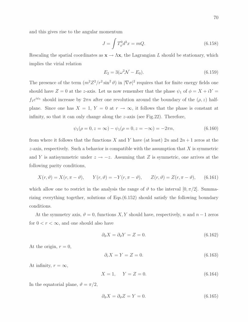
70
and this gives rise to the angular momentum
J =
∫
T 0ϕd
3x = mQ. (6.158)
Rescaling the spatial coordinates as x→ Λx, the Lagrangian L should be stationary, which
implies the virial relation
E2 = 3(ω2N −E0). (6.159)
The presence of the term (m2Z2/r2 sin2 ϑ) in |∇σ|2 requires that for finite energy fields one
should have Z = 0 at the z-axis. Let us now remember that the phase ψ1 of φ = X + iY =
f1eiψ1 should increase by 2πn after one revolution around the boundary of the (ρ, z) half-
plane. Since one has X = 1, Y = 0 at r → ∞, it follows that the phase is constant at
infinity, so that it can only change along the z-axis (see Fig.22). Therefore,
ψ1(ρ = 0, z =∞)− ψ1(ρ = 0, z = −∞) = −2πn, (6.160)
from where it follows that the functions X and Y have (at least) 2n and 2n+ 1 zeros at the
z-axis, respectively. Such a behavior is compatible with the assumption that X is symmetric
and Y is antisymmetric under z → −z. Assuming that Z is symmetric, one arrives at the
following parity conditions,
X(r, ϑ) = X(r, π − ϑ), Y (r, ϑ) = −Y (r, π − ϑ), Z(r, ϑ) = Z(r, π − ϑ), (6.161)
which allow one to restrict in the analysis the range of ϑ to the interval [0, π/2]. Summa-
rizing everything together, solutions of Eqs.(6.152) should satisfy the following boundary
conditions.
At the symmetry axis, ϑ = 0, functions X, Y should have, respectively, n and n− 1 zeros
for 0 < r <∞, and one should also have
∂ϑX = ∂ϑY = Z = 0. (6.162)
At the origin, r = 0,
∂rX = Y = Z = 0. (6.163)
At infinity, r =∞,
X = 1, Y = Z = 0. (6.164)
In the equatorial plane, ϑ = π/2,
∂ϑX = ∂ϑZ = Y = 0. (6.165)

71
C. The sigma model limit
We have succeeded for the first time to solve the equations in the special limit of the
theory obtained by choosing the parameters in the potential (6.137) as
λσ = λφ = β, ησ = 1, γ =1
2β + γ0, (6.166)
such that the potential becomes
U =β
4(|φ|2 + |σ|2 − 1)2 + γ0|φ|2|σ|2. (6.167)
Taking β →∞ enforces the constraint
|φ|2 + |σ|2 = 1 (6.168)
and the theory (6.138) becomes a sigma model,
L = ∂µφ∗∂µφ+ ∂µσ
∗∂µσ − γ0|φ|2|σ|2. (6.169)
This model is simpler than the full theory (6.138). It has less degrees of freedom and no free
parameters, since the value of γ0 can be changed by rescaling the spacetime coordinates.
The field mass Mσ determined by (6.139) reduces now to√γ0, while the mass Mφ becomes
infinite, which means that field degrees of freedom violating the constraint (6.168) are ex-
cluded from the dynamics. The theory therefore contains only one massive particle and two
Goldstone bosons in the spectrum. It is worth noting that N = mn now becomes genuinely
topological charge, invariant under arbitrary smooth field deformations.
It is convenient to use the Lagrange multiplier method by adding to the Lagrangian
(6.169) a term µ(1 − |φ|2 − |σ|2) and varying with respect to φ, σ and µ. Using the same
ansatz (6.148),(6.151) as before gives
∆X =(
γ0Z2 + µ
)
X,
∆Y =(
γ0Z2 + µ
)
Y,
∆Z =
(
m2
r2 sin2 ϑ− ω2 + γ0(X
2 + Y 2) + µ
)
Z. (6.170)
and also
X2 + Y 2 + Z2 − 1 = 0. (6.171)

72
Multiplying the three equations (6.170), respectively, by X, Y, Z and taking their sum and
using the constraint (6.171) one finds the expression for the Lagrange multiplier,
µ = X∆X + Y∆Y + Z∆Z − 2γ0(X2 + Y 2)Z2 − (
m2
r2 sin2 θ− ω2)Z2
− 1
2∆(X2 + Y 2 + Z2), (6.172)
where the second line has been added in order to cancel the second derivatives appearing in
the first line. Inserting this to (6.170), the constraint (6.171) will be imposed automatically
on the solutions, so that it can be excluded from considerations from now on.
The boundary conditions for Eqs.(6.170) are given by Eqs.(6.162)–(6.165). The regularity
condition Z|θ=0,π = 0 imposes the constraint X2 + Y 2 = 1 on the z-axis. In addition, since
at the origin one has Y = 0, the constraint requires that X2 = 1, and so one can choose
X|r=0 = −1 . (6.173)
Since one has X|r=∞ = +1, this will guarantee a non-zero value of n, which is the principal
advantage of the sigma model theory (6.169).
In fact, making sure that the phase of φ winds n 6= 0 times around the contour C is
not simple. This condition can be naturally implemented in toroidal coordinates (2.13),
but these coordinates are somewhat singular at infinity. Spherical or cylindrical coordinates
are better suited for numerics, but the field topology is then determined by zeros of the
X, Y amplitudes (see Eq.(6.160)), whose number cannot be generically prescribed, since
they are able to disappear during numerical iterations. Now, the condition (6.173) enforces
a non-trivial field topology at least in the n = 1 case.
We can now solve the problem. Starting from a field configuration satisfying the boundary
conditions (6.162)–(6.165), (6.173) we numerically iterate it until the convergence is achieved.
The resulting solutions are qualitatively very similar to the generic vortons described in detail
below, and they also agree with the ‘skyrmions’ in the theory of Bose-Einstein condensation
previously obtained in a completely different way by Battye, Cooper and Sutcliffe [17]. The
latter issue will be discussed below in more detail.
D. Explicit vorton solutions
Having obtained vortons in the sigma model limit, we can use them as the starting profiles
in order to iteratively descend from infinite to finite values of β in the potential (6.167), thus

73
relaxing the sigma model condition. After this, we can relax also the conditions (6.166),
thereby recovering vorton solutions within the full original theory (6.138).
In our numerics we use the program FIDISOL (written in Fortran), based on the iter-
ative Newton-Raphson method. A detailed presentation of the FIDISOL code is given in
[152],[150]. In this approach the field equations are discretized on a (r, ϑ) grid with Nr×Nϑ
points, and the resulting system is iterated until convergence is achieved. The grid spacing
in the r-direction is non-uniform, while the values of the grid points in the angular direction
are given by ϑk = (k − 1)π/(2(Nϑ − 1)). Instead of r, a new radial variable x is introduced
which maps the semi-infinite region [0,∞) to the finite interval [0, 1]. There are various
possibilities for such a mapping, a flexible enough choice being x = r/(c + r), where c is
a properly chosen constant. Typical grids for the n = 1 solutions have around 200 × 30
points. The typical numerical error for the solutions is estimated to be of order 10−3. In
addition, the virial relation (6.159) was also monitored. The deviation from unity of the
ratio E2/3(ω2N − E0) is less than 10−3 for most of the solutions we have considered.
0 2 4 6 8 10
-6
-4
-2
0
2
4
6
FIG. 23: Levels of constant amplitude |φ| (closed lines) and phase ψ1 (radial lines, red online)
on the ρ (horizontal direction)–z (vertical direction) plane for the vortex field φ = |φ| exp(iψ1)
corresponding to the vorton solution with n = 1, m = 2, ω = 0.85, λφ = 41.12, λσ = 40, ησ = 1,
γ = 22.3.
As a result, for given values of the parameters λφ, λσ, ησ and γ in the potential, we can
specify the azimuthal winding number m and the frequency ω and obtain a vorton solution.

74
The value of n, the charge Q and energy E are computed from the numerical output. A
complete analysis of the parameter space of solutions is a time consuming task that we
did not aim at. Instead, we analyzed in detail a few particular classes of solutions, which
hopefully reflects the essential properties of the general pattern.
We mainly considered the case where the function X vanishes once at the positive z semi-
axis, which corresponds to the vortex winding number n = 1. The amplitude of the scalar
field φ has in this case one zero located on a circle in the ϑ = π/2 plane. The corresponding
vorton topology can be illustrated by the diagram in Fig.23, where the level lines of the
complex vortex function φ = |φ| exp(iψ1) are shown. The levels of constant amplitude, |φ|,are closed lines encircling the center of the vortex where φ vanishes. Emanating from this
center there are lines of constant phase. The phase, ψ1, increases by 2π after one revolution
around the center.
-1-0.8-0.6-0.4-0.2 0 0.2 0.4 0.6 0.8 1
4
8
12
16
ρ-8
0
8
16
z
-1
-0.5
0
0.5
1
X
-1-0.8-0.6-0.4-0.2 0 0.2 0.4 0.6 0.8 1
3
6
9
ρ-8
0
8
16
z
-1
-0.5
0
0.5
1
Y
FIG. 24: The amplitudes X(ρ, z), Y (ρ, z) for the typical vorton solution; here n = 1, m = 2,
ω = 0.85, λφ = 41.12, λσ = 40, ησ = 1, γ = 22.3.
All vortons have toroidal distributions of the energy density and charge. It seems that
they do not exist for arbitrary values of the parameters of the model but only for some regions
in the parameter space. In Figs. 24, 25 the 3D plots of X, Y, Z and also of |φ| =√X2 + Y 2
for a typical solution with m = 2 are presented. One can see that these functions exhibit
a strong dependence both on ρ and z, with the zero of |φ| located in the z = 0 plane at
R ≃ 0.82.
In Fig. 26, 27 the 2D profiles of X, Y ,Z and |φ| for a typical m = 1 solution for several
values of ϑ are shown; these pictures remain qualitatively the same for higher values of m.

75
0
0.2
0.4
0.6
0.8
1
1.2
4
8
12
16
ρ-8
0
8
16
z
0
0.25
0.5
0.75
1
Z
0 0.1 0.2 0.3 0.4 0.5 0.6 0.7 0.8 0.9 1
4
8
12
16
ρ-8
0
8
16
z
0
0.2
0.4
0.6
0.8
1
|φ|
FIG. 25: The amplitudes Z(ρ, z) and |φ(ρ, z)| for the same solution as in Fig.24.
-1
-0.5
0
0.5
1
0 3 6 9 12 15
r
θ= 0
θ= π/8
θ= π/4
θ= π/2
-0.001
-0.0005
0
0.0005
0.001
4 4.5 5
θ= π/2
0
0.3
0.6
0.9
0 3 6 9 12 15
Y
r
θ= 0
θ= π/8
θ= π/4
θ= π/2
FIG. 26: Profiles of X(r, ϑ), Y (r, ϑ) for fixed ϑ for the n = m = 1 vorton solution with ω = 0.8,
λφ = 33.26, λσ = 32.4, ησ = 1, γ = 18.4.
As seen in these plots, the space can be partitioned into three regions. In the first region,
located near the origin, the functions X, Y, Z present a strong variation, with Y approaching
its extremum. The second region is located inside the vortex, where X stays very close to
zero, while the field Z is almost constant and close to its maximal value. As seen in the
insertion in the first plot, X crosses zero value with a non-zero first derivative, as it should,
since the degree of zero of φ at the vortex center should be one. In the third region, outside
the vortex ring, the fields approach the vacuum values. BothX and Z show strong variations
in a transition domain between second and third regions. We notice also that the value of
X at the origin, which was −1 in the sigma model limit, is now larger, although it stays
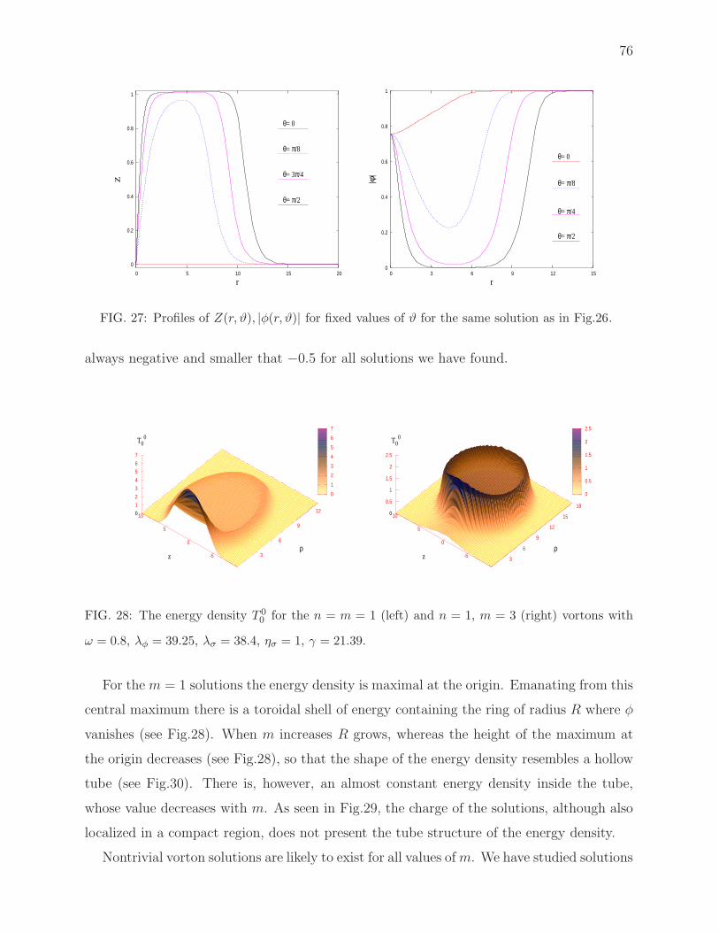
76
0
0.2
0.4
0.6
0.8
1
0 5 10 15 20
Z
r
θ= 0
θ= π/8
θ= 3π/4
θ= π/2
0
0.2
0.4
0.6
0.8
1
0 3 6 9 12 15
|φ|
r
θ= 0
θ= π/8
θ= π/4
θ= π/2
FIG. 27: Profiles of Z(r, ϑ), |φ(r, ϑ)| for fixed values of ϑ for the same solution as in Fig.26.
always negative and smaller that −0.5 for all solutions we have found.
0
1
2
3
4
5
6
7
3
6
9
12
ρ-5
0
5
10
z
0
1
2
3
4
5
6
7
T00
0
0.5
1
1.5
2
2.5
3
6
9
12
15
18
ρ-5
0
5
10
z
0
0.5
1
1.5
2
2.5
T00
FIG. 28: The energy density T 00 for the n = m = 1 (left) and n = 1, m = 3 (right) vortons with
ω = 0.8, λφ = 39.25, λσ = 38.4, ησ = 1, γ = 21.39.
For the m = 1 solutions the energy density is maximal at the origin. Emanating from this
central maximum there is a toroidal shell of energy containing the ring of radius R where φ
vanishes (see Fig.28). When m increases R grows, whereas the height of the maximum at
the origin decreases (see Fig.28), so that the shape of the energy density resembles a hollow
tube (see Fig.30). There is, however, an almost constant energy density inside the tube,
whose value decreases with m. As seen in Fig.29, the charge of the solutions, although also
localized in a compact region, does not present the tube structure of the energy density.
Nontrivial vorton solutions are likely to exist for all values ofm. We have studied solutions

77
0 0.1 0.2 0.3 0.4 0.5 0.6 0.7 0.8 0.9
2
4
6
8
10
12
ρ-5
0
5
10
z
0
0.2
0.4
0.6
0.8
j0(σ)
0 0.1 0.2 0.3 0.4 0.5 0.6 0.7 0.8 0.9
4
8
12
16
ρ-5
0
5
10
z
0
0.2
0.4
0.6
0.8
j0(σ)
FIG. 29: The charge density for the same solutions as in Fig.28.
2000
3000
4000
5000
6000
7000
8000
0.75 0.8 0.85 0.9 0.95 1
ω
E
Q
n=1 m=2
λφ=40.08, λσ=41.12, γ=22.3, ησ=1
FIG. 30: Left: the surface of constant (T 00 = 1.05) energy density for the same n = 1, m = 3 vorton
solution as in Fig.28. It has the structure of a torus containing inside another toroidal surface.
Right: the energy E(ω) and charge Q(ω) for the n = 1,m = 2 vorton solutions.
up to m = 5, but beyond this value the numerical accuracy of our procedure decreases
drastically. The energy of the solutions increases with m, and for solutions with the same
ω one has E(m) < mE(m = 1). All solutions we have found have the ratio R/a between
1 and 1.5, so that the radius of the vortex ring is almost the same as the thickness of the
vortex. The construction of vortons in the thin ring limit, for R ≫ a, remains a numerical
challenge.
Fig.30 (right) shows the energy E and charge Q as functions of the frequency ω for m = 2
vortons. These functions are actually quite similar to those found in the Q-ball case. As

78
one can see, solutions exist for a limited range of frequencies, ω− < ω < ω+. Unfortunately,
the numerical accuracy decreases considerably near the limits of this interval. However, it
seems that both Q(ω) and E(ω) diverge in these limits, as in the Q-ball case.
In analogy with Q-balls, the vortons become large as ω → ω±. However, it is not the
vorton radius R that becomes large, since it appears to be not very sensitive to ω and remains
finite and nonzero when ω approaches its limiting values. It appears that the torus thickness
increases for ω → ω± so that its volume grows, thereby increasing the energy and charge.
Both E and Q assume their minimal values at ω = ωcrit. The dependence E(Q) appears to
be double-valued, very similar to the one shown in Fig.14 for Q-balls, again exhibiting two
branches with a cusp. Solutions with ω < ωcrit are less energetic than those for ω > ωcrit
and with the same Q.
Using again the analogy with Q-balls, it seems likely that only solutions from the lower
branch can be stable, probably those for large enough charge. Stable vortons certainly
exist, perhaps not for all values of the parameters of the potentials, but at least for large
enough values, when the theory approaches the sigma model limit. Vortons in the sigma
model limit are stable, since, as will be discussed below, they can be obtained via 3D energy
minimization [17]. This suggests that they should remain stable at least when they are close
to this limit.
Although we did not study in detail the dependence of the solutions on the parameters
of the potential, one should mention that for ησ ≃ 1 and ω ≃ 0.85 (the values we mainly
considered) we could find solutions only for λφ & 22, while the ratio λφ/λσ was always close
to one. In other words, our vortons are not that far from the sigma model limit, which
suggests that they could be stable.
Vortons with n > 1 also exist, and we were able to construct them for n = 2. For these
solutions there are two concentric rings in the ϑ = π/2 plane where |φ| vanishes. All n = 2
solutions we have found have very large values of λφ, λσ, γ.
Finally, an interesting class of solutions of Eqs.(6.152) is obtained by setting Y = 0, which
means that the phase of φ is trivial and so n = 0. Such solutions have not been discussed
in the literature. Although m 6= 0 in this case, one has N = nm = 0, and so according to
our definition these solutions are not vortons, since they are ‘topologically trivial’. However,
they also have a ring structure, resembling somewhat spinning Q-balls. One can view them
as ‘φ-dressed’ Q-balls made of the complex σ field, the non-renormalizable |σ|6 term in the

79
Q-balls potential being replaced by the interaction with a real scalar field φ, as was first
suggested in Ref.[75].
VII. RING SOLITONS IN NON-RELATIVISTIC SYSTEMS
So far we have been considering relativistic ring solitons that could be relevant in models
of high energy physics. At the same time, similar objects also exist in non-relativistic physics,
and below we shall consider some of them which are most closely related to our previous
discussion.
A famous example of soliton-type toroidal systems is provided by the magnetically con-
fined plasma in the TOKAMAK’s. However, since considering this subject would lead us
far beyond the scope of our present discussion, we shall restrict ourselves to simply giving a
reference to a recent review [28]. In addition, since the external field is necessary to confine
the plasma in this case, this example does not quite fit in with our discussion, because we
are considering closed, self-interacting systems. Another example of plasma confinement,
although somewhat controversial, but which could perhaps be explained by some solitonic
structures, is provided by the phenomenon of ball lightning (see [82] for a bibliography). It
has in fact been conjectured that some analogs of Faddeev-Skyrme solitons in plasma might
be responsible for their existence [67],[63], although we are unaware of any confirmations of
this conjecture via constructing explicit solutions.
Field theory models of condensed matter physics are more closely related to our discus-
sion. As in the relativistic case, they can be either theories with local gauge invariance, as
for example the Ginzburg-Landau theory of superconductivity [77], or models with global
internal symmetries, as in the Gross-Pitaevskii [78], [135], [83] theory of Bose-Einstein con-
densation. It has been conjectured that some analogs of the Faddeev-Skyrme knot solitons
could exist in the multicomponent Ginzburg-Landau models [11]. However, we are again
unaware of any explicit solutions, and moreover, as was discussed above, their existence is
not very plausible, at least in the purely magnetic case. On the other hand, global models
of condensed matter physics do admit ring type solitons.

80
A. Vortons versus ‘skyrmions’ in Bose-Einstein condensates
Surprisingly, it turns out that the described above vortons in the global limit of Witten’s
model can also be considered as solutions of the Gross-Pitaevskii (GP) equation,
i∂Ψa
∂t=
(
−1
2∆ + V (x) +
1
2
∑
b
κab|Ψb|2)
Ψa . (7.174)
This equation, also called nonlinear Schrodinger equation, provides an effective description
of the Bose-Einstein condensates. Here Ψa are the condensate order parameters, V (x) is
the external trapping potential and κab describe interactions between different condensate
components. In the case of a two-component condensate the indices a, b assume values 1, 2.
Let
φ = φ(x), σ = σ(x)eiωt (7.175)
be a solution of the equations (6.142) of the global model of Witten (6.138) in the case where
the parameters in the potential (6.137) are related as
λφ = λση2σ. (7.176)
Then setting
Ψ1 = e−iλφ
4t φ(x), Ψ2 = e
−i“
λφ
4+ ω2
2
”
tσ(x) (7.177)
gives a solution of the GP equation (7.174) in the case where
V (x) = 0, κ11 =λφ2, κ22 =
λσ2, κ12 = κ21 = γ. (7.178)
It follows that any vorton solution satisfying the condition (7.176) (this condition is typically
not difficult to achieve numerically) provides a solutions to the Gross-Pitaevskii equation
and hence can be interpreted in terms of condensed matter physics.
In particular, the condition (7.176) is achieved in the sigma model limit (6.166),(6.168),
in which case one obtains solutions of the GP equation with
V (x) = κ11 = κ22 = 0, κ12 = κ21 = γ0 (7.179)
by setting Ψ1 = φ(x), Ψ2 = e−iω2
2t σ(x). Remarkably, solutions of the GP equation in this
case have been independently studied by Battye, Cooper and Sutcliffe (BCS) [17], so that
we can compare our results in Sec.VIC with theirs. They parametrize the fields as
φ(x) = cosΘ
2einψ , σ(x) = sin
Θ
2eimϕ , (7.180)

81
which exactly coincides with the parametrization (2.32) of the Faddeev-Hopf field. Instead
of directly solving the GP equation, BCS minimize the energy
E2 + E0 =
∫
(|∇φ|2 + |∇σ|2 + γ0|φ|2|σ|2)d3x (7.181)
in a given N sector by keeping fixed the particle number
N =
∫
|σ|2d3x . (7.182)
They call the resulting configurations φN (x), σN (x) ‘skyrmions’ – because Eq.(7.180) agrees
with the skyrmion parametrization (5.123). At first view it is not completely obvious how
these ‘skyrmions’ are related to our vortons φω(x), σω(x) obtained by solving Eqs.(6.170) for
a given ω. However, these are actually the same solutions. In particular, the profiles of the
vortons described in the previous sections, their energy density distributions, are similar to
those for the ‘skyrmions’ given in Ref.[17].
The two different ways to obtain the solutions, either by minimizing the energy or via
solving the equations, are actually equivalent1. This issue has in fact already been discussed
above in the Q-ball context. Q-balls can be obtained either by solving Eq.(5.83), which gives
φω(x), or via minimizing the truncated energy functional E0 + E2 (5.89) with the particle
number N (5.88) fixed, which gives φN (x). Once one knows the value ω = ω(N ), obtained
either with the formula (5.90) or from the virial relation (5.82), the two results can be related
to each other: φω(x) = φω(N )(x) = φN (x).
Similarly, the BCS skyrmions φN (x), σN (x) can be related to our vortons φω(x), σω(x)
by simply establishing the relation ω(N ). The knowledge of ω is important to make sure
that the no radiation condition
ω2 ≤M2σ = γ0 (7.183)
is fulfilled, which is the case for our solutions, while their profiles agree with the features
described by BCS in [17]. This provides an independent confirmation of our numerical
results described in Sec.VIC. Since they can be obtained by the 3D energy minimization,
these solutions are stable.
Apart from the work of BCS there have been other studies of ‘skyrmions’ in Bose-Einstein
condensates [149], [147], [144], [99], [124]. Such solutions have been constructed by numeri-
cally resolving the GP equation for more general choices of V (x) and κab and also for more
1 We thank Richard Battye for explaining this point to us.

82
than two condensate components. Possibilities for an experimental creation and observation
of such objects have also been discussed [146], [145]. In all studies the solutions are typically
presented for the winding numbers n = 1, with the exception of Ref.[144], where results for
n = 2 are reported, although without giving many details. In our language this corresponds
to the double vortons.
B. Spinning rings in non-linear optics – Q-balls as light bullets
Yet another application of the considered above ring solitons arises in the theory of light
propagating in media whose polarization vector ~P depends non-linearly on the electric field
~E . The sourceless Maxwell equations become in this case non-linear and in a number of
important cases they can be reduced to a non-linear Schrodinger (NLS) equation similar to
the Gross-Pitaevskii equation (7.174). For a Kerr medium, when the non-linear part of ~Pis cubic in ~E , the NLS equation has exactly the same structure as Eq.(7.174), but for more
general media it can have different non-linearities. Soliton solutions of this NLS equation
describe non-linear light pulses, sometimes called light bullets, which are very interesting
from the purely theoretical viewpoint and which can actually be observed, as for example in
the optical fibers. Unfortunately, discussing these issues in more detail would lead us away
from our subjects, and so we simply refer to a monograph [6] on optical solitons.
Most of the known solitons of the NLS equation describe plane waves or cylindrical beams
of light [6]. However, solutions describing solitons localized in all three dimensions are also
known, they have been studied by Mihalache et al [125]. These solutions describe spinning
rings, which is very interesting in the context of our discussion.
Mihalache et al consider light pulses travelling in the z direction with a group velocity
V in a medium with cubic and quintic non-linearities. After a suitable rescaling of the
coordinates and fields, the envelope of the pulse, Ψ, satisfies the equation [125]
i∂Ψ
∂z=
(
− ∂2
∂x2− ∂2
∂y2− ∂2
∂ζ2+ |Ψ|4 − |Ψ|2
)
Ψ (7.184)
where ζ = z− V t. Solutions of this equation, numerically constructed in Ref.[125], describe
‘spinning light bullets’. Interestingly, it turns out that these solitons correspond to the
spinning Q-balls already described above.
Specifically, let us rename the variables as z → t, ζ → z and set Ψ = expi(ω2−M2)tφ.

83
Eq.(7.184) then assumes the form
iφ = (−∆ + |φ|4 − |φ|2 +M2 − ω2)φ . (7.185)
Let us now consider Eq.(5.73) describing Q-balls with the potential (5.76). We notice that
rescaling the spacetime coordinates and the field as xµ → Λ1xµ, Φ → Λ2Φ is equivalent to
changing the values of the parameters λ, a in the potential. Therefore, as long as they do
not vanish, one can choose without any loss of generality λ = 1/3, a = 3/2. Setting then
Φ = eiωtφ, Eq.(5.73) assumes the form
− φ− 2iωφ = (−∆ + |φ|4 − |φ|2 +M2 − ω2)φ , (7.186)
with M2 = λb. We see that if φ = 0 then Eq.(7.185) and Eq.(7.186) become identical. They
have therefore the same solutions. We thus conclude that the Q-balls solutions discussed
above in Sec.VA can describe light pulses in non-linear media. The solutions found in
Ref.[125] correspond to the simplest m+, that is non-twisted, even parity Q-balls. Let us
remind that for a given m these solutions can be parametrized by the value of ω varying
within the range ω2−(m) < ω2 < ω2
+ = M2.
Mihalache et al also study the dynamical stability of the solutions by analysing their
small perturbations [125]. Perturbing in Eq.(7.185) the field as φ→ φ + δφ and linearizing
with respect to δφ gives
i ˙δφ = D[φ]δφ , (7.187)
where D[φ] is a linear differential operator. If the spectrum of this operator is known,
D[φ]ξλ = λξλ , (7.188)
then Eq.(7.187) is solved by setting δφ = expiλtξλ. It follows that if there are complex
eigenvalues λ with a negative imaginary part, then the perturbations grow for t → ∞ and
so the background is unstable. Mihalache et al study the spectral problem (7.188) and find
complex eigenvalues for all spinning solitons with m = 2. They also integrate Eq.(7.184) to
trace the full non-linear perturbation dynamics, and they observe that the spinning toroidal
soliton splits into three individual non-spinning spheroidal pieces [125]. However, they find
that the m = 0, 1 solitons can be stable, both at the linear and non-linear levels, if ω is
less than a certain value ω∗(m) < M but still within the domain of the solution existence,
ω−(m) < ω < ω∗(m). According to their results, for m = 0 one has ω∗ = ωcrit, which is the

84
value where E(ω), Q(ω) pass through the minimum (see Fig.14). For m = 1 the stability
region shrinks, since ω∗ < ωcrit, so that not all parts of the less energetic solution branch
(see Fig.14) correspond to stable solutions.
These results are very interesting, since they allow us to draw certain conclusions about
stability of the relativistic Q-balls. Linearizing Eq.(7.186) gives
− δφ− 2iω ˙δφ = D[φ]δφ , (7.189)
whose solution is δφ = expiγtξλ with γ = −ω ±√λ+ ω2. All eigenmodes with complex
λ therefore correspond to complex γ and so to unstable modes. In addition, there could
be unstable modes with real λ < −ω2, since γ would then be complex. As a result, the
relativistic Q-balls have the same unstable modes as their non-relativistic optical counter-
parts (although with different instability growth rates) and perhaps also some additional
instabilities.
It follows that the 2+ spinning Q-balls are unstable, while the 1+ ones, if they belong
to the lower solution branch and their charge is large enough, should be stable (unless they
have negative modes with λ < −ω2). The latter conclusion agrees with the results shown in
Fig.14.
As was said above, Q-balls corresponding to the lower solution branch in Fig.14 cannot
decay into free particles. As we now see, this property does not yet guarantee their stability,
since there can be other decay channels. Their non-relativistic optical counterparts can decay
into several solitonic constituents. In order to see if the same could be true for the relativistic
Q-balls, one should integrate the full time evolutions equation Eq.(7.186). The existence of
negative modes for spinning Q-balls is also suggested by the results of Ref.[10],[16].
The results of Ref.[125] have been generalized in Refs.[126],[127] to describe the case of
light pulses with two independent polarizations and also for more general non-linearities of
the medium.
C. Moving vortex rings
For the sake of completeness, we would also like to consider another well known type of
ring solitons: moving vortex rings in continuous media. Although they are stabilized by the
interaction with the medium and not by intrinsic forces, their structure can be quite similar
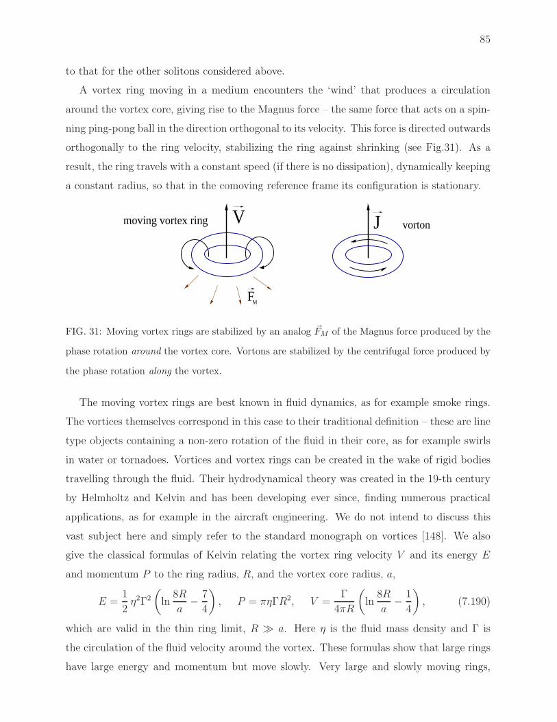
85
to that for the other solitons considered above.
A vortex ring moving in a medium encounters the ‘wind’ that produces a circulation
around the vortex core, giving rise to the Magnus force – the same force that acts on a spin-
ning ping-pong ball in the direction orthogonal to its velocity. This force is directed outwards
orthogonally to the ring velocity, stabilizing the ring against shrinking (see Fig.31). As a
result, the ring travels with a constant speed (if there is no dissipation), dynamically keeping
a constant radius, so that in the comoving reference frame its configuration is stationary.
V
FM
Jmoving vortex ring vorton
FIG. 31: Moving vortex rings are stabilized by an analog ~FM of the Magnus force produced by the
phase rotation around the vortex core. Vortons are stabilized by the centrifugal force produced by
the phase rotation along the vortex.
The moving vortex rings are best known in fluid dynamics, as for example smoke rings.
The vortices themselves correspond in this case to their traditional definition – these are line
type objects containing a non-zero rotation of the fluid in their core, as for example swirls
in water or tornadoes. Vortices and vortex rings can be created in the wake of rigid bodies
travelling through the fluid. Their hydrodynamical theory was created in the 19-th century
by Helmholtz and Kelvin and has been developing ever since, finding numerous practical
applications, as for example in the aircraft engineering. We do not intend to discuss this
vast subject here and simply refer to the standard monograph on vortices [148]. We also
give the classical formulas of Kelvin relating the vortex ring velocity V and its energy E
and momentum P to the ring radius, R, and the vortex core radius, a,
E =1
2η2Γ2
(
ln8R
a− 7
4
)
, P = πηΓR2, V =Γ
4πR
(
ln8R
a− 1
4
)
, (7.190)
which are valid in the thin ring limit, R ≫ a. Here η is the fluid mass density and Γ is
the circulation of the fluid velocity around the vortex. These formulas show that large rings
have large energy and momentum but move slowly. Very large and slowly moving rings,

86
which could perhaps be described by some version of hydrodynamics of magnetized plasma,
are observed in Sun’s atmosphere.
1. Moving vortex rings in the superfluid helium
Moving vortex rings exist also in the superfluid helium, where they are created by moving
impurities [140] (see [170] for a survey of defects in helium). It turns out that large rings
in helium can be well described by the classical hydrodynamics. However, in the generic
case their adequate description should be quantum. The superfluid helium can be approx-
imately modeled by a weakly interacting Bose-Einstein condensate (although in reality the
interactions in helium are not weak, see e.g. [23]), in which case vortices can be described
by solutions of the Gross-Pitaevskii equation (7.174). In the simplest case one can consider
the one-component version of this equation, which, upon setting V (x) = 0, κ11 = κ and
Ψ1 ≡ e−iκ2t Ψ reduces to
2i∂Ψ
∂t=(
−∆ + κ(|Ψ|2 − 1))
Ψ . (7.191)
Rescaling coordinates and time one can set κ = 1, if it is positive. Choosing Ψ = einϕf(ρ)
gives
f ′′ +1
ρf ′ − n2
ρ2f = (f 2 − 1)f , (7.192)
whose solution with the boundary conditions f(0) = 0 and f(∞) = 1 describes a global
vortex with n quanta of circulation [78].
Solutions of the GP equation (7.191) describing moving vortex rings and their various
properties have been comprehensively analyzed by P.H. Roberts and collaborators in a series
of articles written over the last 25 years, of which we only mention Refs.[81], [97], [24], [22],
[21]. The fundamental vortex ring solutions have been numerically obtained by Jones and
Roberts [97] by setting
Ψ = Ψ(ρ, z − V t), (7.193)
such that Ψ(ρ, z) satisfies the equation
− i2V ∂zΨ =(
−∆ + (|Ψ|2 − 1))
Ψ . (7.194)
They imposed the reflection condition Ψ(ρ, z) = Ψ(ρ,−z)∗ and also the asymptotic condi-
tions for large r,
ℜ(Ψ) = 1 +O(r−3), ℑ(Ψ) = O(r−2). (7.195)

87
Numerically integrating Eq.(7.194), they obtained a family of solutions labeled by V ∈(0, Vmax), where Vmax = 1/
√2 is the speed of sound in the dimensionless units chosen. For
small V the solutions have ring profiles: the function Ψ vanishes at a point (R, 0) in the
(ρ, z) plane while its phase increases by 2π after one revolution around this point, so that Ψ
has the ‘vorton topology’ (see Fig.22). When V is small, the radius of the ring, R, as well
as its energy and momentum,
E =1
2
∫(
|∇Ψ|2 +1
2(|Ψ|2 − 1)2
)
d3x ,
P3 = ℑ∫
(Ψ∗ − 1)∂zΨ d3x, (7.196)
are large, and in the leading order they agree with the classical Kelvin formulas (7.190) [81].
As V increases, E, P3 and R all decrease, and the following relation holds,
V =∂E
∂P3
. (7.197)
The ring radius R vanishes for V = V0 ≈ 0.62 and for V0 < V < Vmax solutions change their
character and describe acoustic excitations in helium, called in [97] rarefaction pulses, in
which case Ψ no longer has zeroes . The energy and momentum diverge when V approaches
0, Vmax, and they both assume their minimal values for some V = Vcrit ≈ 0.657. The
functions E(V ) and P3(V ) exhibit therefore qualitatively the same behaviour as E(ω) and
Q(ω) for the Q-balls (see Fig.14). The function E(P3) shows the two-branch structure with
a cusp, similarly to E(Q) in Fig.14. The moving rings belong to the lower branch, which
suggests that they could be stable. Their perturbative stability has been demonstrated by
Berloff and Roberts [24], who also studied the ring creation by solving the GP equation for
a superfluid flow around a moving solid sphere [22] and showed that rings are created in its
wake, provided that its velocity exceeds some critical value.
The moving ring solutions have been generalized for a non-zero trapping potential V (x)
in the GP equation (see [110] for a review) and for the two-component condensate case
[20]. An interesting solution of the GP equation describing a non-linear superposition of a
straight vortex and a vortex ring encircling it and moving along it, somewhat similar to the
‘hoop’ solution shown in Fig.19, has been presented by Berloff in [21].
One may also wonder whether the vortex ring solutions could be generalized within a
relativistic field theory (as is the case for the vortex solution of Eq.(7.192)). In fact, the

88
answer to this question is affirmative, since taking a solution Ψ(ρ, z) of Eq.(7.194) and setting
φ = eiV (z±t)Ψ(ρ, z) (7.198)
and also σ = 0 solves Eqs.(6.142) of Witten’s model for λφ = 2. However, since Ψ → 1 at
infinity, it follows that φ→ eiV (z±t) in this limit, which corresponds to a massless Goldstone
radiation. The relativistic analogs of the moving vortex rings are therefore radiative solutions
and their total energy is infinite.
2. Moving magnetic rings
An interesting example of moving ring solitons, found by Cooper [41] and studied also by
Sutcliffe [159], arises in ferromagnetic systems whose dynamics is described in the continuum
limit by the Landau-Lifshitz equation
∂na
∂t= ǫabcn
b∆nc. (7.199)
Here na is a unit three-vector, nana = 1, giving the local orientation of the magnetization.
The temporal evolution defined by the Landau-Lifshitz equation preserves the value of the
energy
E =1
4
∫
(∂kna)2d3x . (7.200)
In addition, it does not change the momentum,
Pi =1
2
∫
ǫijk(xjBk)d3x, (7.201)
where Bi = 12ǫijkFjk and Fjk is defined as in the Faddeev-Skyrme model by Eq.(2.2). The
number of spin flips,
N =1
2
∫
(1− n3)d3x, (7.202)
is also preserved by the evolution; for this number to be finite one should have n3 = 1 at
infinity. Since the theory contains a unit vector field, it can be characterized by the topo-
logical index of Hopf defined by the same equation (2.9) as in the Faddeev-Skyrme model.
An axially symmetric field configuration with a non-zero Hopf charge can be parametrized
exactly as in Eq.(2.10) (with n = 1),
n1 + in2 = sin Θ(ρ, z) expi[mϕ− ψ(ρ, z)], n3 = cos Θ(ρ, z). (7.203)

89
The energy density then has a ring structure and the Hopf charge is N = m. Using this to
calculate the momentum (7.201) shows that its z-component does not vanish,
Pz =1
4
∫
ρ(∂zΘ∂ρψ − ∂ρΘ∂zψ)d3x . (7.204)
This means that if one uses (7.203) as the initial data for the Landau-Lifshitz equation,
then this data set will have a non-zero initial momentum. To verify this assertion, Sutcliffe
[159] directly integrates the Landau-Lifshitz equation to reconstruct the temporal dynamics
of the ring. For largely arbitrary functions Θ(ρ, z), ψ(ρ, z) in (7.203) he then sees the whole
ring configuration drift with an almost constant velocity along the z-axis. He also observes
that the phase of n1 + in2 increases as a linear function of the distance travelled by the ring,
so that there are internal rotations in the ring as it moves.
These empirical features can be understood by making the following ansatz for the dy-
namical fields [41],
n1 + in2 = sin Θ(ρ, z−V t) expi[mϕ+ωt−ψ(ρ, z−V t)], n3 = cos Θ(ρ, z−V t), (7.205)
with constant V, ω. Inserting this ansatz to the Landau-Lifshitz equation (7.199), the t, ϕ
variables separate and the problem reduces to the two dimensional elliptic problem for
Θ(ρ, z), ψ(ρ, z),
∆Θ = (ω + V ∂zψ) sin Θ +
[
(∂ρψ)2 + (∂zψ)2) +m2
ρ2
]
sin Θ cosΘ,
sin Θ∆ψ = −V ∂zΘ− 2 cosΘ[∂ρΘ∂ρψ + ∂zΘ∂zψ]. (7.206)
This problem is in fact very much similar to that in the vorton case. This can be seen
by applying the same change of variables which was used to rewrite the Faddeev–Skyrme
model (2.1) in the CP 1 form (2.29), na = Φ†τaΦ , with Φ†Φ = 1. This parametrization of
the system allows one to write down a simple Lagrangian for the Landau-Lifshitz equation
(7.199),
L = iΦ†∂tΦ−1
4(∂kn
a)2 + µ(Φ†Φ− 1), (7.207)
where µ is the Lagrange multiplier. One can parametrize Φ exactly in the same way as in
the vorton case,
Φ =
X + iY
Zeiωt+imϕ
.

90
Inserting this to the Lagrangian (7.207) and varying with respect toX, Y, Z, µ gives equations
similar to Eqs.(6.170) for vortons in the sigma model limit. These equations can be solved
with the same boundary conditions (6.162)–(6.165) for X, Y, Z as for vortons. On the other
hand, setting X + iY = cos(Θ/2)eiψ and Z = sin(Θ/2), as in Eq.(7.180), gives again
Eqs.(7.206).
Fixing m one can solve the equations for suitable input values of ω, V . Having obtained
the solutions, one can calculate E(ω, V ), N (ω, V ) and P3(ω, V ). Alternatively, instead of
solving the equations, one can minimize the energy E with fixed N , P3. Having found the
minimal value E(N , P3), one can reconstruct ω, V as [41],[159]
ω =∂E
∂N , V =∂E
∂P3. (7.208)
Cooper [41] and Sutcliffe [159] choose the latter approach: they minimize the energy with
fixed N , P3 for several values of m = N . Their numerics converge to non-trivial configu-
rations Θ(ρ, z), ψ(ρ, z), inserting which to (7.205) gives dynamical rings travelling with a
constant velocity. Fixing all other parameters, the ring velocity decreases with growing m.
In fact, these rings also have an angular momentum, J = mN , but apparently this
feature is not so essential for their stabilization as it is for vortons, since solutions with
m = N = J = 0 also exist and do not exhibit any particular features as compared to the
solutions with m 6= 0 [159]. Similarly to the other moving ring solitons discussed above,
magnetic rings are stabilized by a Magnus-type force produced by the phase circulation
around the vortex core and directed outwards, orthogonally to the velocity (see Fig.31).
The magnetic rings are stable not only against shrinking but also with respect to all other
deformations – since they can be obtained via the 3D energy minimization [159].
VIII. CONCLUDING REMARKS
We have reviewed the known field theory solutions describing stationary vortex loops.
From the physical point of view, loops of magnetic flux would perhaps be the most in-
teresting. However, as we have seen, almost all explicit solutions describe vortex loops in
global field theories, which are effective theories with a relatively limited range of applica-
bility. Perspectives for generalizing these solutions in the context of gauge field theory do
not look very promising at the moment, at least as far as knot solitons are concerned. The

91
best known static knot solitons, Faddeev-Skyrme knots, do not seem to admit immediate
gauge field theory generalizations, unless one makes additional physical assumptions to fix
the charges in the Protogenov-Verbus formula. Such assumptions can be made, as shows
the example of Schmid and Shaposhnikov. However this requires a rather exotic physical
environment.
The non-Abelian monopole and sphaleron rings are very interesting theoretically, how-
ever, they are presumably unstable. It is therefore unclear whether they can find important
physical applications. Summarizing, the existence of knots – magnetic vortex loops sta-
bilized against shrinking by internal stresses – does not seem to be very plausible in the
context of physically interesting relativistic gauge field theories.
Perhaps gauged vortons have more chances to exist. As we have seen, their global coun-
terparts do exist as stationary, non-radiating field theory objects. Already for these global
vortons an additional analysis to study the structure of the parameter space is needed. A
natural problem to address would be their analysis in the thin ring limit, for large values of
the azimuthal winding number m, when the ring radius is much larger than the vortex core
thickness. One can expect that the field theory solutions in this limit should agree with the
effective macroscopic description. This limit, however, is difficult to explore numerically,
since the vorton fields are then almost everywhere constant, except for a narrow ring region
containing all the field gradients. It is difficult to properly adjust the grid in this case, so
that some other numerical methods are necessary, as perhaps the multi-domain spectral
method [80]. Is seems also that some other methods are necessary to study solutions with
n > 1.
Yet another interesting related problem would be to find vortons with three winding
numbers. We know that the phase of φ winds around the vortex core, while that of σ winds
along the ring, the corresponding winding numbers being n andm. However, nothing forbids
the phase of σ to wind both around the core and along the ring, as does the phase of the
twisted Q-balls, in which case one would need a third integer, k, counting the windings of σ
around the vortex core. Constructing vortons with k 6= 0 remains a challenge.
A very important open problem related to all vortons is their dynamical stability analysis.
This problem can be handled either by studying the spectrum of small field fluctuations
around the vorton background, or by looking for vorton negative modes within the energy
minimization method, or by reconstructing the full temporal evolution of the perturbed
92
vorton configuration. Stable vortons definitely exist, at least in the sigma model limit, but
in the generic case their stability should be studied.
Generalizing global vortons within gauge field theory does not seem to be impossible.
In theories where all the internal symmetries are gauged, as in Witten’s model (6.136), all
spinning phases of the fields can be gauged away, so that if the fields are stationary and
axisymmetric, these symmetries are manifest. In this case the surface integral formula (4.66)
for the angular momentum applies, providing higher chances for J to vanish due to the fast
asymptotic falloff of the fields. Although the example of spinning gauged Q-balls shows that
spinning is possible in local theories, it seems that vortons have better chances to exist in
models with both local and global internal symmetries. Such models contain gauge fields,
such that one can have magnetic vortices, but the gauge freedom is not enough to gauge
away all the phases of the scalars. The symmetries of the fields are therefore not manifest
and the surface integral formula does not apply, in which case the angular momentum should
normally be non-zero.
For example, it would be natural to analyze the existence of stationary vortons in a
half gauged version of Witten’s modes obtained by coupling the two scalars in Eq.(6.138)
to a U(1) gauge field. Such solutions could then perhaps be generalized within the fully
gauged U(1)×U(1) Witten’s modes to confirm the existence of stationary loops made of
superconducting cosmic strings – the idea first put forward more than 20 years ago.
However, a real challenge would be to construct stationary superconducting loops in
Standard Model. There are indications that this might be possible. The electroweak sector
of Standard Model contains stationary current carrying vortices – superconducting strings
[166]. Their stability has been studied so far only in the semilocal limit, where the SU(2)
gauge field decouples and the current becomes global [73],[72], and it has been found that
sufficiently short pieces of strings are perturbatively stable [76]. This suggests that small
loops made of these strings may also be stable. If such loops could be constructed for the
physical value of the weak mixing angle, this would give stable solitons in Standard Model.
For the sake of completeness, having in mind possible applications of vortex loops in
astrophysics and cosmology, it is also interesting to mention the effects of gravity on these
solutions. On general grounds, one expects all known ring solitons to admit self-gravitating
generalizations with essentially the same properties as in the zero gravity limit, at least for
small enough values of the gravitational coupling constant. However, the soliton structure
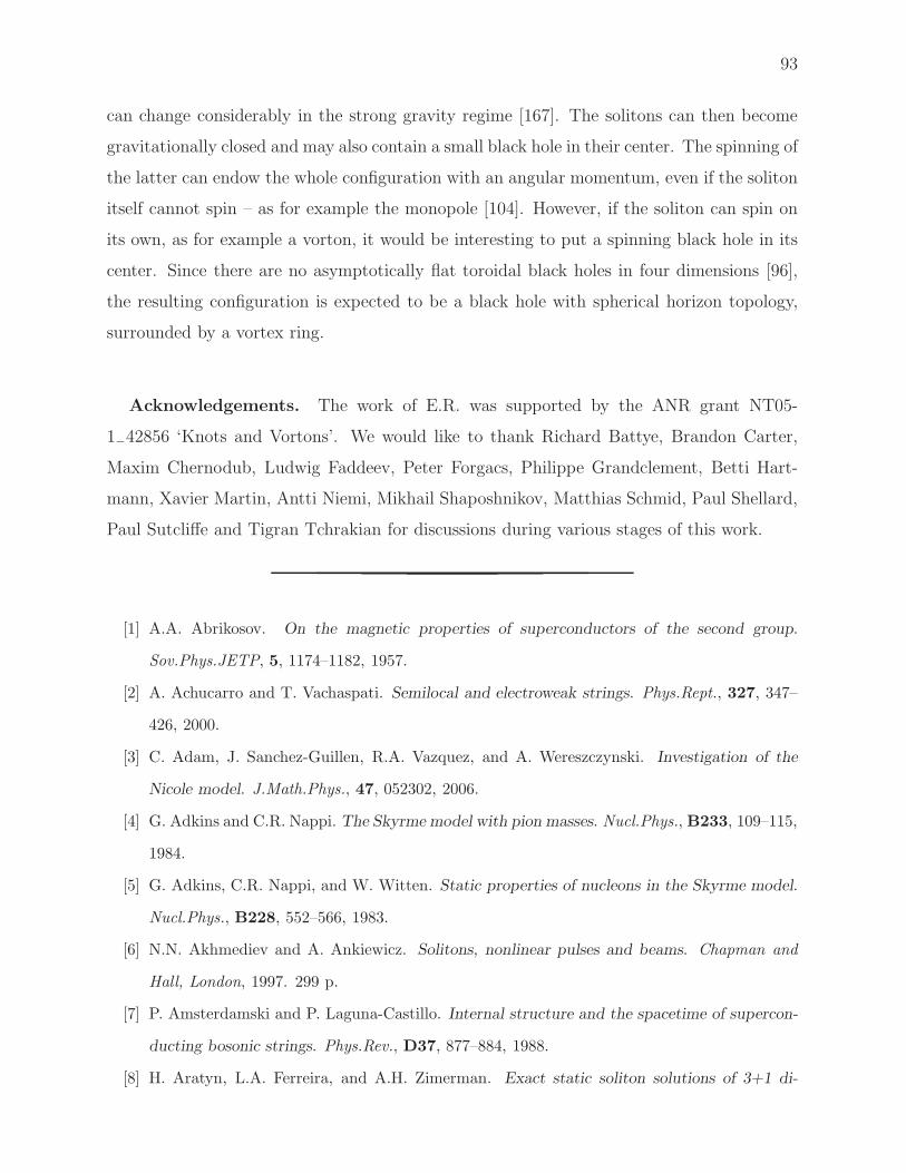
93
can change considerably in the strong gravity regime [167]. The solitons can then become
gravitationally closed and may also contain a small black hole in their center. The spinning of
the latter can endow the whole configuration with an angular momentum, even if the soliton
itself cannot spin – as for example the monopole [104]. However, if the soliton can spin on
its own, as for example a vorton, it would be interesting to put a spinning black hole in its
center. Since there are no asymptotically flat toroidal black holes in four dimensions [96],
the resulting configuration is expected to be a black hole with spherical horizon topology,
surrounded by a vortex ring.
Acknowledgements. The work of E.R. was supported by the ANR grant NT05-
1−42856 ‘Knots and Vortons’. We would like to thank Richard Battye, Brandon Carter,
Maxim Chernodub, Ludwig Faddeev, Peter Forgacs, Philippe Grandclement, Betti Hart-
mann, Xavier Martin, Antti Niemi, Mikhail Shaposhnikov, Matthias Schmid, Paul Shellard,
Paul Sutcliffe and Tigran Tchrakian for discussions during various stages of this work.
[1] A.A. Abrikosov. On the magnetic properties of superconductors of the second group.
Sov.Phys.JETP, 5, 1174–1182, 1957.
[2] A. Achucarro and T. Vachaspati. Semilocal and electroweak strings. Phys.Rept., 327, 347–
426, 2000.
[3] C. Adam, J. Sanchez-Guillen, R.A. Vazquez, and A. Wereszczynski. Investigation of the
Nicole model. J.Math.Phys., 47, 052302, 2006.
[4] G. Adkins and C.R. Nappi. The Skyrme model with pion masses. Nucl.Phys., B233, 109–115,
1984.
[5] G. Adkins, C.R. Nappi, and W. Witten. Static properties of nucleons in the Skyrme model.
Nucl.Phys., B228, 552–566, 1983.
[6] N.N. Akhmediev and A. Ankiewicz. Solitons, nonlinear pulses and beams. Chapman and
Hall, London, 1997. 299 p.
[7] P. Amsterdamski and P. Laguna-Castillo. Internal structure and the spacetime of supercon-
ducting bosonic strings. Phys.Rev., D37, 877–884, 1988.
[8] H. Aratyn, L.A. Ferreira, and A.H. Zimerman. Exact static soliton solutions of 3+1 di-
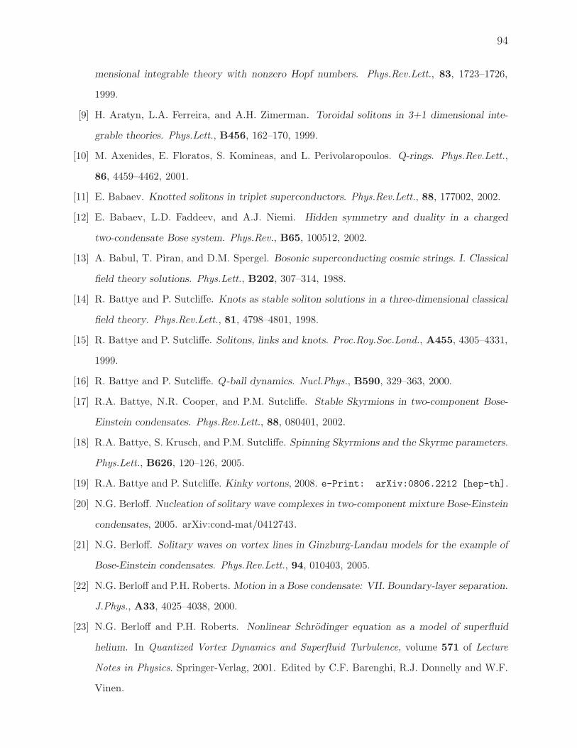
94
mensional integrable theory with nonzero Hopf numbers. Phys.Rev.Lett., 83, 1723–1726,
1999.
[9] H. Aratyn, L.A. Ferreira, and A.H. Zimerman. Toroidal solitons in 3+1 dimensional inte-
grable theories. Phys.Lett., B456, 162–170, 1999.
[10] M. Axenides, E. Floratos, S. Komineas, and L. Perivolaropoulos. Q-rings. Phys.Rev.Lett.,
86, 4459–4462, 2001.
[11] E. Babaev. Knotted solitons in triplet superconductors. Phys.Rev.Lett., 88, 177002, 2002.
[12] E. Babaev, L.D. Faddeev, and A.J. Niemi. Hidden symmetry and duality in a charged
two-condensate Bose system. Phys.Rev., B65, 100512, 2002.
[13] A. Babul, T. Piran, and D.M. Spergel. Bosonic superconducting cosmic strings. I. Classical
field theory solutions. Phys.Lett., B202, 307–314, 1988.
[14] R. Battye and P. Sutcliffe. Knots as stable soliton solutions in a three-dimensional classical
field theory. Phys.Rev.Lett., 81, 4798–4801, 1998.
[15] R. Battye and P. Sutcliffe. Solitons, links and knots. Proc.Roy.Soc.Lond., A455, 4305–4331,
1999.
[16] R. Battye and P. Sutcliffe. Q-ball dynamics. Nucl.Phys., B590, 329–363, 2000.
[17] R.A. Battye, N.R. Cooper, and P.M. Sutcliffe. Stable Skyrmions in two-component Bose-
Einstein condensates. Phys.Rev.Lett., 88, 080401, 2002.
[18] R.A. Battye, S. Krusch, and P.M. Sutcliffe. Spinning Skyrmions and the Skyrme parameters.
Phys.Lett., B626, 120–126, 2005.
[19] R.A. Battye and P. Sutcliffe. Kinky vortons, 2008. e-Print: arXiv:0806.2212 [hep-th].
[20] N.G. Berloff. Nucleation of solitary wave complexes in two-component mixture Bose-Einstein
condensates, 2005. arXiv:cond-mat/0412743.
[21] N.G. Berloff. Solitary waves on vortex lines in Ginzburg-Landau models for the example of
Bose-Einstein condensates. Phys.Rev.Lett., 94, 010403, 2005.
[22] N.G. Berloff and P.H. Roberts. Motion in a Bose condensate: VII. Boundary-layer separation.
J.Phys., A33, 4025–4038, 2000.
[23] N.G. Berloff and P.H. Roberts. Nonlinear Schrodinger equation as a model of superfluid
helium. In Quantized Vortex Dynamics and Superfluid Turbulence, volume 571 of Lecture
Notes in Physics. Springer-Verlag, 2001. Edited by C.F. Barenghi, R.J. Donnelly and W.F.
Vinen.
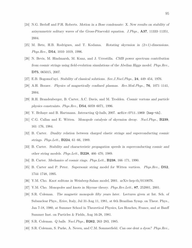
95
[24] N.G. Berloff and P.H. Roberts. Motion in a Bose condensate: X. New results on stability of
axisymmetric solitary waves of the Gross-Pitaevskii equation. J.Phys., A37, 11333–11351,
2004.
[25] M. Betz, H.B. Rodrigues, and T. Kodama. Rotating skyrmion in (2+1)-dimensions.
Phys.Rev., D54, 1010–1019, 1996.
[26] N. Bevis, M. Hindmarsh, M. Kunz, and J. Urrestilla. CMB power spectrum contribution
from cosmic strings using field-evolution simulations of the Abelian Higgs model. Phys.Rev.,
D75, 065015, 2007.
[27] E.B. Bogomol’nyi. Stability of classical solutions. Sov.J.Nucl.Phys., 24, 449–454, 1976.
[28] A.H. Boozer. Physics of magnetically confined plasmas. Rev.Mod.Phys., 76, 1071–1141,
2004.
[29] R.H. Brandenberger, B. Carter, A.C. Davis, and M. Trodden. Cosmic vortons and particle
physics constraints. Phys.Rev., D54, 6059–6071, 1996.
[30] Y. Brihaye and B. Hartmann. Interacting Q-balls, 2007. arXiv:0711.1969 [hep-th].
[31] C.G. Callan and E. Witten. Monopole catalysis of skyrmion decay. Nucl.Phys., B239,
161–176, 1984.
[32] B. Carter. Duality relation between charged elastic strings and superconducting cosmic
strings. Phys.Lett., B224, 61–66, 1989.
[33] B. Carter. Stability and characteristic propagation speeds in superconducting cosmic and
other string models. Phys.Lett., B228, 466–470, 1989.
[34] B. Carter. Mechanics of cosmic rings. Phys.Lett., B238, 166–171, 1990.
[35] B. Carter and P. Peter. Supersonic string model for Witten vortices. Phys.Rev., D52,
1744–1748, 1995.
[36] Y.M. Cho. Knot solitons in Weinberg-Salam model, 2001. arXiv:hep-th/0110076.
[37] Y.M. Cho. Monopoles and knots in Skyrme theory. Phys.Rev.Lett., 87, 252001, 2001.
[38] S.R. Coleman. The magnetic monopole fifty years later. Lectures given at Int. Sch. of
Subnuclear Phys., Erice, Italy, Jul 31-Aug 11, 1981, at 6th Brazilian Symp. on Theor. Phys.,
Jan 7-18, 1980, at Summer School in Theoretical Physics, Les Houches, France, and at Banff
Summer Inst. on Particles & Fields, Aug 16-28, 1981.
[39] S.R. Coleman. Q balls. Nucl.Phys., B262, 263–283, 1985.
[40] S.R. Coleman, S. Parke, A. Neveu, and C.M. Sommerfield. Can one dent a dyon? Phys.Rev.,

96
D15, 544–545, 1977.
[41] N.R. Cooper. Propagating magnetic vortex rings in ferromagnets. Phys.Rev.Lett., 82, 1554–
1557, 2001.
[42] E.J. Copeland, D. Haws, M. Hindmarsh, and N. Turok. Dynamics of and radiation from
superconducting strings and springs. Nucl.Phys., B306, 908–930, 1988.
[43] E.J. Copeland, M. Hindmarsh, and N. Turok. Dynamics of superconducting cosmic strings.
Phys.Rev.Lett., 58, 1910–1913, 1987.
[44] F. Paccetti Correia and M.G. Schmidt. Q balls: some analytical results. Eur.Phys.Journ.,
C21, 181–191, 2001.
[45] R.L. Davis. Semitopological solitons. Phys.Rev., D38, 3722–3730, 1988.
[46] R.L. Davis and E.P.S. Shellard. The physics of vortex superconductivity. Phys.Lett., B207,
404–410, 1988.
[47] R.L. Davis and E.P.S. Shellard. The physics of vortex superconductivity. 2. Phys.Lett.,
B209, 485–490, 1988.
[48] R.L. Davis and E.P.S. Shellard. Cosmic vortons. Nucl.Phys., B323, 209–224, 1989.
[49] H.J. de Vega. Closed vortices and the Hopf index in classical field theory. Phys.Rev., D18,
2945–2951, 1978.
[50] J.J. Van der Bij and E. Radu. On rotating regular nonabelian solutions. Int.J.Mod.Phys.,
A17, 1477–1490, 2002.
[51] J.J. Van der Bij and E. Radu. Magnetic charge, angular momentum and negative cosmological
constant. Int.J.Mod.Phys., A18, 2379–2393, 2003.
[52] G.H. Derrick. Comments on nonlinear wave equations as models for elementary particles.
J.Math.Phys., 5, 1252–1254, 1964.
[53] L. Dittmann, T. Heinzl, and A. Wipf. A lattice study of the Faddeev-Niemi action.
Nucl.Phys.Proc.Suppl., B106, 649–651, 2002.
[54] R.J. Donnelly. Quantized vortices in helium II. Cambridge University Press, 1991. 346 p.
[55] C.G. Doudoulakis. On vortices and rings in extended Abelian models. Physica, D234, 1–10,
2007.
[56] C.G. Doudoulakis. On vortices and solitons in Goldstone and Abelian-Higgs models, 2007.
arXiv:0709.3709 [hep-ph].
[57] C.G. Doudoulakis. Search of axially symmetric solitons. Physica, D228, 159–165, 2007.
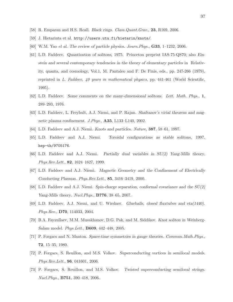
97
[58] R. Emparan and H.S. Reall. Black rings. Class.Quant.Grav., 23, R169, 2006.
[59] J. Hietarinta et al. http://users.utu.fi/hietarin/knots/.
[60] W.M. Yao et al. The review of particle physics. Journ.Phys., G33, 1–1232, 2006.
[61] L.D. Faddeev. Quantization of solitons, 1975. Princeton preprint IAS-75-QS70; also Ein-
stein and several contemporary tendencies in the theory of elementary particles in Relativ-
ity, quanta, and cosmology, Vol.1, M. Pantaleo and F. De Finis, eds., pp. 247-266 (1979),
reprinted in L. Faddeev, 40 years in mathematical physics, pp. 441-461 (World Scientific,
1995).
[62] L.D. Faddeev. Some comments on the many-dimensional solitons. Lett. Math. Phys., 1,
289–293, 1976.
[63] L.D. Faddeev, L. Freyhult, A.J. Niemi, and P. Rajan. Shafranov’s virial theorem and mag-
netic plasma confinement. J.Phys., A35, L133–L140, 2002.
[64] L.D. Faddeev and A.J. Niemi. Knots and particles. Nature, 387, 58–61, 1997.
[65] L.D. Faddeev and A.J. Niemi. Toroidal configurations as stable solitons, 1997.
hep-th/9705176.
[66] L.D. Faddeev and A.J. Niemi. Partially dual variables in SU(2) Yang-Mills theory.
Phys.Rev.Lett., 82, 1624–1627, 1999.
[67] L.D. Faddeev and A.J. Niemi. Magnetic Geometry and the Confinement of Electrically
Conducting Plasmas. Phys.Rev.Lett., 85, 3416–3419, 2000.
[68] L.D. Faddeev and A.J. Niemi. Spin-charge separation, conformal covariance and the SU(2)
Yang-Mills theory. Nucl.Phys., B776, 38–65, 2007.
[69] L.D. Faddeev, A.J. Niemi, and U. Wiedner. Glueballs, closed fluxtubes and eta(1440).
Phys.Rev., D70, 114033, 2004.
[70] B.A. Fayzullaev, M.M. Musakhanov, D.G. Pak, and M. Siddikov. Knot soliton in Weinberg-
Salam model. Phys.Lett., B609, 442–448, 2005.
[71] P. Forgacs and N. Manton. Space-time symmetries in gauge theories. Commun.Math.Phys.,
72, 15–35, 1980.
[72] P. Forgacs, S. Reuillon, and M.S. Volkov. Superconducting vortices in semilocal models.
Phys.Rev.Lett., 96, 041601, 2006.
[73] P. Forgacs, S. Reuillon, and M.S. Volkov. Twisted superconducting semilocal strings.
Nucl.Phys., B751, 390–418, 2006.

98
[74] P. Forgacs and M.S. Volkov. On the existence of knot solitons in gauge field theory, 2002.
unpublished.
[75] R. Friedberg, T.D. Lee, and A. Sirlin. A class of scalar-field soliton solutions in three space
dimensions. Phys.Rev., D13, 2739–2761, 1976.
[76] J. Garaud and M.S. Volkov. Stability analysis of the twisted superconducting electroweak
strings. Nucl.Phys., B799, 430–455, 2008.
[77] V.L. Ginzburg and L.D. Landau. On the theory of superconductivity. Zh.Eksp.Teor.Fiz.,
20, 1064, 1950.
[78] V.L. Ginzburg and L.P. Pitaevskii. On the theory of superfluidity. Sov.Phys.JETP, 34,
858–861, 1958.
[79] J. Gladikowski and M. Hellmund. Static solitons with non-zero Hopf number. Phys.Rev.,
D56, 5194–5199, 1997.
[80] P. Grandclement and J. Novak. Spectral methods for numerical relativity, 2007.
arXiv:0706.2286 [gr-qc].
[81] J. Grant and P.H. Roberts. Motion in a Bose condensate III. The structure and effective
masses of charged and uncharged impurities. J.Phys., A7, 260–279, 1974.
[82] B. Greenwood. Ball lightning bibliography. www.project1947.com/shg/bl−db.html.
[83] E.P. Gross. Structure of quantized vortex. Nuovo Cimento, 20, 454–477, 1961.
[84] B. Hartmann and B. Carter. The logarithmic equation of state for superconducting cosmic
strings, 2008. arXiv:0803.0266 [hep-th].
[85] B. Hartmann, B. Kleihaus, and J. Kunz. Dyons with axial symmetry. Mod.Phys.Lett., A15,
1003–1012, 2000.
[86] D. Haws, M. Hindmarsh, and N. Turok. Superconducting strings or springs ? Phys.Lett.,
B209, 255–261, 1988.
[87] I. Hen and M. Karliner. Spontaneous breaking of rotational symmetry in rotating solitons:
A toy model of excited nucleons with high angular momentum. Phys.Rev., D77, 116002,
2008.
[88] M. Heusler, N. Straumann, and M. Volkov. On rotational excitations and axial deformations
of BPS monopoles and Julia-Zee dyons. Phys.Rev., D58, 105021, 1998.
[89] J. Hietarinta and P. Salo. Faddeev-Hopf knots: Dynamics of linked un-knots. Phys.Lett.,
B451, 60–67, 1999.

99
[90] J. Hietarinta and P. Salo. Ground state in the Faddeev-Skyrme model. Phys.Rev., D62,
081701, 2000.
[91] C.T Hill, H.M. Hodges, and M.S. Turner. Bosonic superconducting cosmic strings. Phys.Rev.,
D37, 263–282, 1988.
[92] R.H. Hobart. On the instability of a class of unitary field model. Proc.Phys.Soc., 82, 201–203,
1963.
[93] K. Huang and R. Tipton. Vortex excitations in the Weinberg-Salam theory. Phys.Rev., D23,
3050–3057, 1981.
[94] T. Ioannidou, B. Kleihaus, and J. Kunz. Spinning gravitating skyrmions. Phys.Lett., B643,
213–220, 2006.
[95] J. Jaykka, J. Hietarinta, and P. Salo. Investigation of the stability of Hopfions in the two-
component Ginzburg-Landau model. Phys.Rev., B77, 094509, 2008.
[96] J.L.Friedman, K. Schliech, and D.M. Witt. Topological censorship. Phys.Rev.Lett., 71,
1486–1489, 1993.
[97] C.A. Jones and P.H. Roberts. Motion in a Bose condensate: IV. Axisymmetric solitary
waves. J.Phys., A15, 2599–2619, 1982.
[98] B. Julia and A. Zee. Poles with both magnetic and electric charges in nonabelian gauge
theory. Phys.Rev., D11, 2227–2232, 1975.
[99] Y. Kawaguchi, M. Nitta, and M. Ueda. Knots in a spinor Bose-Einstein condensate, 2008.
arXiv:0802.1968 [cond-mat.other].
[100] B. Kleihaus and J. Kunz. A monopole antimonopole solution of the SU(2) Yang-Mills- Higgs
model. Phys.Rev., D61, 025003, 2000.
[101] B. Kleihaus, J. Kunz, and M. Leissner. Sphalerons, antisphalerons and vortex rings, 2008.
arXiv:0802.3275 [hep-th].
[102] B. Kleihaus, J. Kunz, and M. List. Rotating boson stars and Q-balls. Phys.Rev., D72,
064002, 2005.
[103] B. Kleihaus, J. Kunz, M. List, and I. Schaffer. Rotating boson stars and Q-balls II: negative
parity and ergoregions, 2007. arXiv:0712.3742 [gr-qc].
[104] B. Kleihaus, J. Kunz, and F. Navarro-Lerida. Rotating black holes with monopole hair.
Phys.Lett., B599, 294–300, 2004.
[105] B. Kleihaus, J. Kunz, and U. Neemann. Gravitating stationary dyons and rotating vortex

100
rings. Phys.Lett., B623, 171–178, 2005.
[106] B. Kleihaus, J. Kunz, and Y. Shnir. Monopoles, antimonopoles and vortex rings. Phys.Rev.,
D68, 101701, 2003.
[107] B. Kleihaus, J. Kunz, and Y. Shnir. Monopole-antimonopole chains and vortex rings.
Phys.Rev., D70, 065010, 2004.
[108] F.R. Klinkhamer and N.S. Manton. A saddle point solution in the Weinberg-Salam theory.
Phys.Rev., D30, 2212–2220, 1984.
[109] Y. Koma, H. Suganuma, and H. Toki. Flux-tube ring and glueball properties in the dual
Ginzburg-Landau theory. Phys.Rev., D60, 074024, 1999.
[110] S. Komineas. Vortex rings and solitary waves in trapped Bose-Einstein condensates.
Eur.Phys.J. Special Topics, 147, 133–152, 2007.
[111] A. Kundu and Yu.P. Rybakov. Closed-vortex-type solitons with Hopf index. J.Phys., A15,
269–275, 1982.
[112] A. Kusenko. Small Q-balls. Phys.Lett., B404, 285–290, 1997.
[113] A. Kusenko. Solitons in the supersymmetric extensions of the standard model. Phys.Lett.,
B405, 108–113, 1997.
[114] A. Kusenko and M. Shaposhnikov. Supersymmetric Q-balls as dark matter. Phys.Lett.,
B418, 46–54, 1998.
[115] K. Lee, J.A. Stein-Schabes, R. Watkins, and L.M. Widrow. Gauged Q-balls. Phys.Rev.,
D39, 1665–1673, 1989.
[116] T. D. Lee and Y. Pang. Nontopological solitons. Phys.Rept., 221, 251–350, 1992.
[117] A.J. Leggett. Bose-Einstein condensation in the alkali gazes: Some fundamental concepts.
Rev.Mod.Phys., 73, 307–356, 2001.
[118] Y. Lemperiere and E. P. S. Shellard. Vorton existence and stability. Phys.Rev.Lett., 91,
141601, 2003.
[119] F. Lin and Y. Yang. Existence of energy minimizers as stable knotted solitons in the Faddeev
model. Comm.Math.Phys., 249, 273–303, 2004.
[120] V.G. Makhankov, Y.P. Rybakov, and V.I. Sanyuk. The Skyrme model, Fundamentals, Meth-
ods, Applications. Springer-Verlag, Berlin, 1993.
[121] N. Manton and P. Sutcliffe. Topological Solitons. Cambridge University Press, 2004. 493 p.
[122] C.J.A.P. Martins and E.P.S. Shellard. Vorton formation. Phys.Rev., D57, 7155–7176, 1998.

101
[123] U.G. Meissner. Toroidal solitons with unit Hopf charge. Phys.Lett., B154, 190–192, 1985.
[124] M. Metlitski and A.R. Zhitnitsky. Vortex Rings in two Component Bose-Einstein Conden-
sates. JHEP, 06, 017, 2004.
[125] D. Mihalache, D. Mazilu, L.C. Crasovan, I. Towers, A.V. Buryak, B.A. Malomed, L. Torner,
J.P. Torres, and F. Lederer. Stable spinning optical solitons in three dimensions.
Phys.Rev.Lett., 88, 073902, 2002.
[126] D. Mihalache, D. Mazilu, L.C. Crasovan, I. Towers, B.A. Malomed, A.V. Buryak, L. Torner,
and F. Lederer. Stable three-dimensional spinning optical solitons supported by competing
quadratic and cubic nonlinearities. Phys.Rev., E66, 016613, 2002.
[127] D. Mihalache, D. Mazilu, I. Towers, B.A. Malomed, and F. Lederer. Stable spatiotemporal
spinning solitons in a bimodal cubic-quintic medium. Phys.Rev., E67, 056608, 2003.
[128] A.D. Nicole. Solitons with non-vanishing Hopf index. J.Phys., 4, 1363–1369, 1978.
[129] H.B. Nielsen and P. Olesen. Vortex line models for dual strings. Nucl.Phys., B61, 45–61,
1973.
[130] A.J. Niemi, K. Palo, and S. Virtanen. (Meta)stable closed vortices in (3+1)+dimensional
gauge theories with an extended Higgs sector. Phys.Rev., D61, 085020, 2000.
[131] V. Paturyan, E. Radu, and D.H. Tchrakian. Rotating regular solutions in Einstein-Yang-
Mills-Higgs theory. Phys.Lett., B609, 360–366, 2005.
[132] P. Peter. Superconducting cosmic string: Equation of state for spacelike and timelike current
in the neutral limit. Phys.Rev., D45, 1091–1102, 1992.
[133] B.M.A.G. Piette, B.J. Schroers, and W. Zakrzewski. Dynamics of baby skyrmions.
Nucl.Phys., B439, 205–238, 1995.
[134] B.M.A.G. Piette and D.H. Tchrakian. Static solutions in the U(1) gauged Skyrme model.
Phys.Rev., D62, 025020, 2000.
[135] L.P. Pitaevskii. Vortex lines in an imperfect Bose gas. Sov.Phys.JETP, 13, 451–454, 1961.
[136] A.M. Polyakov. Particle spectrum in quantum field theory. JETP Lett., 20, 194–195, 1974.
[137] A.P. Protogenov and V.A. Verbus. Energy bounds of linked vortex states. JETP Lett., 76,
53–55, 2002.
[138] E. Radu and D.H. Tchrakian. Spinning U(1) gauged skyrmions. Phys.Lett., B632, 109–113,
2006.
[139] R. Rajaraman. Solitons and Instantons. North Holland, Amsterdam, 1982. 418 p.
102
[140] G.W. Rayfield and F. Reif. Quantized vortex rings in superfluid helium. Phys.Rev., A136,
1194–1208, 1964.
[141] J. Ren, R. Li, and Y. Duan. Inner topological structure of Hopf invariant. Journ.Math.Phys.,
48, 073502, 2007.
[142] V.A. Rubakov. On the electroweak theory at high fermion density. Prog.Theor.Phys., 75,
366–385, 1986.
[143] V.A. Rubakov and A.N. Tavkhelidze. Stable anomalous states of superdense matter in gauge
theories. Phys.Lett., B165, 109–112, 1985.
[144] J. Ruostekoski. Stable particlelike solitons with multiply-quantized vortex lines in Bose-
Einstein condensates. Phys.Rev., A70, 041601, 2004.
[145] J. Ruostekoski and Z. Dutton. Engineering vortex rings and systems for controlled studies
of vortex interactions in Bose-Einstein condensates. Phys.Rev., A72, 063626, 2005.
[146] J. Ruostekoski and J. R. J.R. Anglin. Creating vortex rings and three-dimensional skyrmions
in Bose-Einstein condensates. Phys.Rev.Lett., 86, 3934–3937, 2001.
[147] J. Ruostekoski and J. R. J.R. Anglin. Monopole core instability and Alice rings in spinor
Bose- Einstein condensates. Phys. Rev. Lett., 91, 190402, 2003.
[148] P.G. Saffman. Vortex dynamics. Cambridge University Press, 1992. 311 p.
[149] C.M. Savage and J. Ruostekoski. Energetically stable particle-like Skyrmions in a trapped
Bose-Einstein condensate. Phys.Rev.Lett., 91, 010403, 2003.
[150] M. Schauder, R. Weiß and W. Schonauer. The CADSOL Program Package, Universitat
Karlsruhe Interner Bericht Nr. 46/92 , 1992.
[151] M. Schmid and M. Shaposhnikov. Anomalous Abelian solitons. Nucl.Phys., B775, 365–389,
2007.
[152] W. Schonauer and R. Weiß. The Fidisol blackbox solver. J. Comput. Appl. Math., 27,
279–297, 1989.
[153] S.V. Shabanov. An effective action for monopoles and knot solitons in Yang-Mills theory.
Phys.Lett., B458, 322–330, 1999.
[154] S.V. Shabanov. Yang-Mills theory as an Abelian theory without gauge fixing. Phys.Lett.,
B463, 263–272, 1999.
[155] Y. Shnir. Electromagnetic interaction in the system of multimonopoles and vortex rings.
Phys.Rev., D72, 055016, 2005.

103
[156] Ya.M. Shnir. Magnetic monopoles. Springer-Verlag, Berlin-Heidelberg, 2005. 532 p.
[157] T.H.R. Skyrme. A nonlinear field theory. Proc.Roy.Soc.Lond., A260, 127–138, 1961.
[158] P. Sutcliffe. Knots in the Skyrme-Faddeev model, 2007. arXiv:0705.1468 [hep-th].
[159] P. Sutcliffe. Vortex rings in ferromagnets, 2007. arXiv:0707.1383 [cond-mat.mes-hall].
[160] G. ’t Hooft. Magnetic monopoles in unified gauge theories. Nucl.Phys., B79, 276–284, 1974.
[161] C.H. Taubes. The existence of a non-minimal solution to the SU(2) Yang-Mills-Higgs equa-
tions on R3. Commun.Math.Phys., 86, 257–298, 1982.
[162] W.H. Thomson. On vortex motion. Trans.R.Soc.Edin., 25, 217–260, 1867.
[163] A.F. Vakulenko and L.V. Kapitansky. Stability of solitons in S2 in the nonlinear σ-model.
Sov.Phys.Dokl., 24, 433–434, 1979.
[164] P. van Baal and A. Wipf. Classical gauge vacua as knots. Phys.Lett., B515, 181–184, 2001.
[165] A. Vilenkin and E.P.S. Shellard. Cosmic Strings and Other Topological Defects. Cambridge
University Press, 1994. 517 p.
[166] M.S. Volkov. Superconducting electroweak strings. Phys.Lett., B644, 203–207, 2007.
[167] M.S. Volkov and D.V. Gal’tsov. Gravitating non-Abelian solitons and black holes with Yang-
Mills fields. Phys.Rep., 319, 1–83, 1999.
[168] M.S. Volkov and E. Wohnert. Spinning Q-balls. Phys.Rev., D66, 085003, 2002.
[169] M.S. Volkov and E. Wohnert. On the existence of spinning solitons in gauge field theory.
Phys.Rev., D67, 105006, 2003.
[170] G.E. Volovik. The Universe in a helium droplet. Oxford University Press, 2003. 507 p.
[171] R.S. Ward. Hopf solitons on S3 and R3, 1998. hep-th/9811176.
[172] R.S. Ward. The interaction of two Hopf solitons. Phys.Lett., B473, 291–296, 2000.
[173] R.S. Ward. Hopf solitons from instanton holonomy, 2001. hep-th/0108082.
[174] R.S. Ward. Stabilizing textures with magnetic fields. Phys.Rev., D66, 041701, 2002.
[175] R.S. Ward. Skyrmions and Faddeev-Hopf solitons. Phys.Rev., D70, 061701, 2004.
[176] R.S. Ward. Hopf solitons on the lattice. J.Phys., A39, L105–L109, 2006.
[177] E. Witten. Superconducting strings. Nucl.Phys., B249, 557–592, 1985.
[178] V.A. Zakharov and E.A. Kuznetsov. Hamiltonian formalism for nonlinear waves. Phys.Usp.,
40, 1087–1116, 1997.