Knapsack

0/1 Knapsack algorithm comparisonJacek Dzikowski

Illinois Institute of Technologye-mail: [email protected]

Abstract:

The goal of this report was to implement compare four different 0/1 Knapsack algorithms (brute force,backtracking, best-first branch and bound, and dynamic programming) in terms of their performance on varioussets of data. All algorithms were first programmed using object-oriented programming language (C++) and thencarefully tested with specially generated data sets. The results that were gathered during these tests served as abasis for further analysis, discussion and drawing conclusions concerning the performance characteristics of allfour algorithms. Final discussion leads to the conclusion that backtracking method seems to be the best in certainconditions, while Brute Force is evidently the least efficient algorithm as expected.

J ACEK D Z I K O W S K I

www.iit.edu/~dzikjac e-mail: [email protected]

2

Introduction

The 0/1 Knapsack problem is an optimisation problem. The idea is to select an optimal (most valuable) subset ofthe set of all items (each characterised by its value and weight), knowing the maximum weight limit. Solutions tothis problem are widely used for example in loading/delivery applications.

There are several existing approaches/algorithms to this problem. Obviously, and it will be proved later, all ofthem led to the same result, but the methods used are different. In this report the focus will be on the followingfour 0/1 Knapsack algorithms:q Brute Force – find optimal result by trying all existing item combinations,q Backtracking – use a State Space concept – find optimal solution by traversing the State Space tree and

backtracking when a node is not promising,q Best-First Branch and Bound – use a State Space concept – expand the nodes with highest bound first (best-

first) to find the optimal solution,q Dynamic Programming – create and use the dynamic programming matrix to find the optimal solution.

Obviously, using a different method implies difference in performance (usually also range of application). 0/1Knapsack algorithms are no different. All four presented algorithmic approaches should be different both interms of run-time and resources consumption.

My approach to verify this statement and to find out which algorithm is the best (in given circumstances) was toprepare a computer program (using an object-oriented programming language) that allows to run all algorithmson a particular set of data and measure the algorithm performance.

This program would be run in order to collect necessary data (run-time, array sizes, queue sizes, etc.) which willbe further used to analyse the overall performance of 0/1 Knapsack algorithms.

Due to its nature, the Brute Force algorithm is expected to perform the worst [O(2number of items )]. On the other sidethe performance of Backtracking and Best-First Branch and Bound algorithms should be much better, howeverits performance is strongly dependant upon the input data set. Similar remark applies also to the DynamicProgramming approach, however here memory utilisation is predictable (more specific the matrix size ispredictable). Of course the cost of increased performance is in memory utilisation (recursive calls stack, queuesize or dynamic programming array).

Materials and methods

The implementation was prepared using Visual C++ object-oriented environment. Aside of four 0/1 Knapsackalgorithms it includes an easy to use menu, data set generation, performance measurement and file loadingmechanisms. The menu allows specifying whether the user wants to load a ready made data file or create a newone (by specifying number of items, range of weights, type of data and seed). Once a file is prepared (either justgenerated or already existing) another menu allows choosing an algorithm to use. Furthermore the number oftrials can be adjusted to eliminate zero-length run-times and increase the accuracy.

Algorithm implementation:q Brute Force – this algorithm checks all the possible combinations of items by means of a simple for loop

(from 1 to 2number of items ). It utilises the binary representation of every combination/number from 1 to 2number of

items (computed recursively) to calculate total profit and weight. At the same time total weight is being

verified whether it exceeds the Weight Limit or not. If so, total profit is 0. Once a better combination isdiscovered it is stored as a result.

q Backtracking – this algorithm utilises the idea of virtual State Space tree. Every branch in this treecorresponds to one combination. Each node is expanded only if it is promising (additional function isimplemented for this purpose) otherwise the algorithm backtracks. It is a recursive algorithm – recursivecalls are executed only if the node is promising. Total weight and profit is computed accordingly and theoptimal solution stored similarly like in Brute Force algorithm.

q Best-First Branch and Bound – another State Space tree algorithm, however its implementation and ideasare different. There is no recursion in my implementation of this algorithm. Instead it uses a priority queueto traverse along the State Space tree (and to keep several states in memory – unlike Brute Force andBacktracking algorithms, which keep only one state at the time). Here the nodes are enqueued into the queue



3

only if their bound (computed by means of additional function) is satisfactory/promising (highest bound isthe priority). The implementation utilises a simple while loop [while (Queue not empty)] to obtain the result.Optimal solution is computed similarly as in previous algorithms.

q Dynamic Programming – here a two-dimensional dynamic programming is used (of size number ofitems*weight limit). It stores solutions to all sub-problems that may constitute an optimal solution. Thealgorithm starts by filling first row and column with zeros and then filling it until it finds the optimalsolution as in other dynamic programming algorithms. Filling the array is realised by means of two nestedloops and two if statements. Optimal profit will be then the last (bottom right) entry in the array andcorresponding weight is then extracted by a single while loop.

The implementation of main functions representing these algorithms is presented in the appendices. Pseudo-codethat was a basis for the implementation of Backtracking and Best-First Branch and Bound algorithm can befound in [1].

ObjectsThe program defines several objects:q item – a structure for storing item information (value, weight, value/weight ratio). Items are further stored in

an Item_Array,q node – a class defining a State Space tree node for Backtracking and Best-First Branch and Bound

algorithms. It defines such variables as Profit, Weight, Level and Bound together with functions to set andextract these values. Additionally it defines overloading of relational operators for queueing purposes,

q test – main object containing the array of items and implementation of all four algorithms together with theirsupporting functions and other auxiliary functions (loading data, sorting, etc,).

q generator – a class defining the data set generator,q userInterface – a class defining the user interface (menus, timer).

SortingAlgorithms other than Brute Force require its input (item) array to be sorted according to the value/weight ratioof the item. I implemented Quick Sort algorithm for this task. Sorting is done before the run-time is computed,hence it does not influence the overall performance measurement.

Data sets:The generator mechanism that is included in the program generates a data file of the following format:

Number_Of_ItemsItem_Number Item_Value Item_Weight (one to a line)Weight_Limit10 1 12 43 2 8 48 3 62 46 4 2 11 5 7 48 6 87 97 7 27 5 8 77 59 9 24 85 10 60 6145

The generator allows specifying the size of the sample and the range of values. Additionally, data can eitherstrongly correlated or uncorrelated.

Measurements:All algorithms were tested using the same sets of data (generated with parameters: number of items n, range ofvalues 100, type of data 1/3, seed 300). Number of items (5, 10, 15, 20, 30, 40, 80, 160) and type of data(Uncorrelated/Strongly Correlated) - variable. I decided to expand the range of number of items due to the fact,that Brute Force algorithm was not working for inputs with n>30 (my decimal to binary algorithm was notworking with data structures better than long).

All tests (excluding Brute Force for n>10) were repeated 100 000 times to obtain better accuracy.



4

Metrics:q Run-time – calculated for every algorithm; measured in seconds using timer implemented in class

userInterafce (it stores the system time at the start and at the end of running the algorithm and then computesthe difference),

q Number of expanded nodes/combinations – a metric used to show how many nodes/combinations analgorithm has to check in order to find the right solution. Used with Backtracking, Best-First Branch andBound and Brute Force algorithms,

q Queue size – maximum priority queue size that was reached during the execution of the Best-First Branchand Bound algorithm. Memory utilisation metric,

q Number of recursive calls – maximum number of recursive calls that are not finished yet during theexecution of the Backtracking algorithm. Memory utilisation metric.

q Dynamic Programming array size – Memory utilisation metric.

Compiler and experimental environment:The program was compiled in Visual C++ 6.0 environment and was run under MS Windows 98 operatingsystem.

Results

Performance results:The performance results that I obtained after running tests for each algorithm with uncorrelated data are shownin Table 1. Additionally the solutions to the 0/1 Knapsack problem for the given uncorrelated data sets arepresented in Table 2.

Best run-time performance results are indicated in Table 1 with bold face.

No. of items 5 10 15 20 30 40 80 160

Brute Force 0.000017 0.000241 0.010288 0.940000 611.1500 N/A N/A N/ACombinations/recursive calls

2^5/5 2^10/10 2^15/15 2^20/20 2^30/30 N/A N/A N/A

Backtracking 0.000003 0.000004 0.000007 0.000008 0.000028 0.000049 0.000080 0.000094Expandednodes/maxrecursive calls

11/6 11/6 31/16 41/21 57/23 101/31 333/81 199/82

Best-FirstBranch andBound

0.000007 0.000007 0.000011 0.000012 0.000058 0.000071 0.000130 0.000220

Expandednodes/queuesize

11/1 11/1 31/1 41/1 101/3 57/5 333/11 199/3

DynamicProgramming

0.000012 0.000021 0.000046 0.000167 0.000170 0.005700 0.007700 0.022000

Array size 5*102 10*131 15*234 20 *307 30*442* 40*558 80*1112 160*2240

Table 1. Performance comparison of various 0/1 Knapsack algorithms (uncorrelated data).

No. of items 5 10 15 20 30 40 80 160

Profit 161 340 541 655 899 1179 2316 4863Weight 96 130 232 293 438 597 1109 2239

Table 2 . Optimal profit weight results for different number of items (uncorrelated data).

The graphical representation of the runtime results for uncorrelated data is shown on Figure 1. Since thedifferences are significant the graph is plotted in using semi-logarithmic scale.



5

Figure 1. Runtime results (uncorrelated data) – semi-logarithmic scale.

The performance results that I obtained after running tests for each algorithm with strongly correlated data areshown in Table 3. Additionally the solutions to the 0/1 Knapsack problem for the given strongly correlated datasets are presented in Table 4.

Best run-time performance results are indicated in Table 3 with bold face.

No. of items 5 10 15 20 30 40 80 160

Brute Force 0.000033 0.000249 0.105400 0.930000 621.9700 N/A N/A N/ACombinations/recursive calls

2^5/5 2^10/10 2^15/15 2^20/20 2^30/30 N/A N/A N/A

Backtracking 0.000008 0.000009 0.000014 0.000220 0.000600 0.000143 0.009120 0.011000Expandednodes/maxrecursive calls

45/6 61/11 117/16 739/21 2145/31 1925/41 1918155/81

124305/161

Best-FirstBranch andBound

0.000015 0.000019 0.000035 0.000248 0.060000 0.000538 0.868400 0.045600

Expandednodes/queuesize

45/4 61/6 117/10 739/30 2147/86 1925/24 1918155/13263

124305/612

DynamicProgramming

0.000012 0.000024 0.000043 0.000720 0.002200 0.00600 0.013200 0.000170

Array size 5*102 10*145 15*211 20*299 30*495 40*630 80*1183 160*2241

Table 3. Performance comparison of various 0/1 Knapsack algorithms (strongly correlated data).

No. of items 5 10 15 20 30 40 80 160

Profit 117 193 287 398 644 839 1602 3130Weight 87 143 207 298 494 629 1182 2240

Table 4. Optimal profit weight results for different number of items (strongly correlated data).

20 40 60 80 100 120 140 160

10-5

10-4

10-3

10-2

10-1

100

101

102

Number of items

Exe

cutio

n tim

e [s

]

Execution time = f(number of items) - Uncorrelated data

--- Brute Force- - Dynamic Programming-.- Best-First Branch and Bound... Backtracking



6

The graphical representation of the runtime results for strongly correlated data is shown on Figure 2. Since thedifferences are significant the graph is plotted in using semi-logarithmic scale.

Figure 2. Runtime results (strongly correlated data) – semi-logarithmic scale.

Uncorrelated data vs. Strongly correlated data – Run-time:The graphs below depict the difference (or lack of difference) in run-time performance for a particular algorithmwhen applying it too different types of data.

q Brute Force

Figure 3. Uncorrelated data vs. correlated data run-time (Brute Force).

20 40 60 80 100 120 140 16010

-5

10-4

10-3

10-2

10-1

100

101

102

Number of items

Exe

cutio

n tim

e [s

]Execution time = f(number of items) - Strongly correlated data


5 10 15 20 25 30

100

200

300

400

500

600

Number of items

Exe

cutio

n tim

e [s

] (so

lid -

unc

orre

late

d, d

ashe

d -

corr

elat

ed)

Normal scale

5 10 15 20 25 30

10-4

10-3

10-2

10-1

100

101

102

Number of items

Exe

cutio

n tim

e [s

] (so

lid -

unc

orre

late

d, d

ashe

d -

corr

elat

ed)

Semilog scale



7

q Backtracking

Figure 4. Uncorrelated data vs. correlated data run-time (Backtracking).

q Best-First Branch and Bound

Figure 5. Uncorrelated data vs. correlated data run-time (Best-First Branch and Bound).

20 40 60 80 100 120 140 160

1

2

3

4

5

6

7

8

9

10

11x 10

-3

Number of items

Exe

cutio

n tim

e [s

] (so

lid -

unc

orre

late

d, d

ashe

d -

corr

elat

ed)

Normal scale

20 40 60 80 100 120 140 160

10-5

10-4

10-3

10-2

Number of items

Exe

cutio

n tim

e [s

] (so

lid -

unc

orre

late

d, d

ashe

d -

corr

elat

ed)

Semilog scale

20 40 60 80 100 120 140 160

0.1

0.2

0.3

0.4

0.5

0.6

0.7

0.8

Number of items

Exe

cutio

n tim

e [s

] (so

lid -

unc

orre

late

d, d

ashe

d -

corr

elat

ed)

Normal scale

20 40 60 80 100 120 140 160

10-5

10-4

10-3

10-2

10-1

Number of items

Exe

cutio

n tim

e [s

] (so

lid -

unc

orre

late

d, d

ashe

d -

corr

elat

ed)

Semilog scale



8

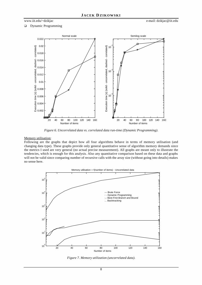
q Dynamic Programming

Figure 6. Uncorrelated data vs. correlated data run-time (Dynamic Programming).

Memory utilisation:Following are the graphs that depict how all four algorithms behave in terms of memory utilisation (andchanging data type). These graphs provide only general quantitative sense of algorithm memory demands sincethe metrics I used are very general (no actual precise measurement). All graphs are meant only to illustrate thetendencies, which is enough for this analysis. Also any quantitative comparison based on these data and graphswill not be valid since comparing number of recursive calls with the array size (without going into details) makesno sense here.

Figure 7. Memory utilization (uncorrelated data).

20 40 60 80 100 120 140 160

0.002

0.004

0.006

0.008

0.01

0.012

0.014

0.016

0.018

0.02

0.022

Number of items

Exe

cutio

n tim

e [s

] (so

lid -

unc

orre

late

d, d

ashe

d -

corr

elat

ed)

Normal scale

20 40 60 80 100 120 140 160

10- 4

10- 3

10- 2

Number of items

Exe

cutio

n tim

e [s

] (so

lid -

unc

orre

late

d, d

ashe

d -

corr

elat

ed)

Semilog scale

20 40 60 80 100 120 140 16010

0

101

102

103

104

105

Number of items

Memory utilisation = f(number of items) - Uncorrelated data




9

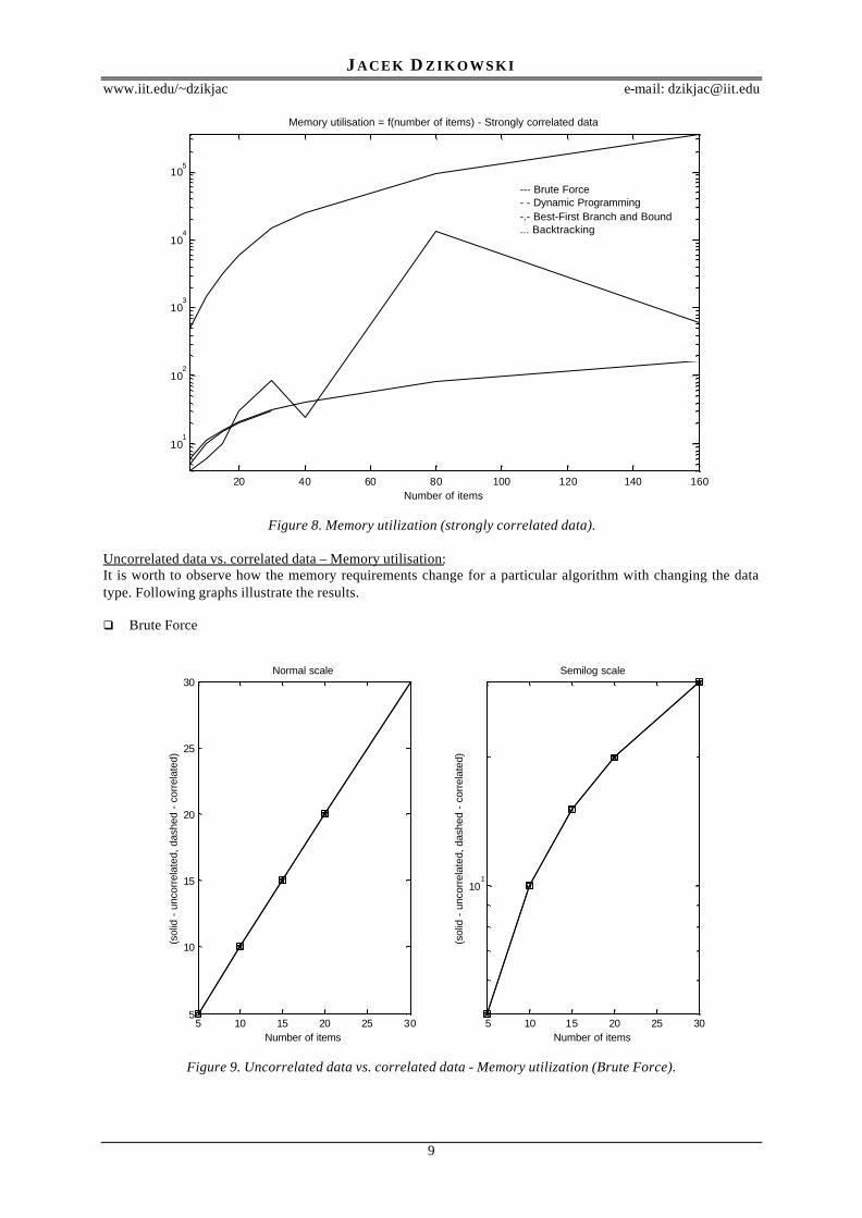
Figure 8. Memory utilization (strongly correlated data).

Uncorrelated data vs. correlated data – Memory utilisation:It is worth to observe how the memory requirements change for a particular algorithm with changing the datatype. Following graphs illustrate the results.

q Brute Force

Figure 9. Uncorrelated data vs. correlated data - Memory utilization (Brute Force).

20 40 60 80 100 120 140 160

101

102

103

104

105

Number of items

Memory utilisation = f(number of items) - Strongly correlated data


5 10 15 20 25 305

10

15

20

25

30

Number of items

(sol

id -

unc

orre

late

d, d

ashe

d -

corr

elat

ed)

Normal scale

5 10 15 20 25 30

101

Number of items

(sol

id -

unc

orre

late

d, d

ashe

d -

corr

elat

ed)

Semilog scale



10

Figure 10. Uncorrelated data vs. correlated data - Memory utilization (Backtracking).

Figure 11. Uncorrelated data vs. correlated data - Memory utilization (Best-First Branch and Bound).

20 40 60 80 100 120 140 160

20

40

60

80

100

120

140

160

Number of items

(sol

id -

unc

orre

late

d, d

ashe

d -

corr

elat

ed)

Normal scale

20 40 60 80 100 120 140 160

101

102

Number of items

(sol

id -

unc

orre

late

d, d

ashe

d -

corr

elat

ed)

Semilog scale

20 40 60 80 100 120 140 160

2000

4000

6000

8000

10000

12000

Number of items

(sol

id -

unc

orre

late

d, d

ashe

d -

corr

elat

ed)

Normal scale

20 40 60 80 100 120 140 16010

0

101

102

103

104

Number of items

(sol

id -

unc

orre

late

d, d

ashe

d -

corr

elat

ed)

Semilog scale



11

Figure 12. Uncorrelated data vs. correlated data - Memory utilization (Dynamic Programming).

Discussion

The first and obvious conclusion that appears when we look at the data in Tables 2 and 4 is that all algorithmsindeed provide the same exact solution to the 0/1 Knapsack problem. The differences are in performance andresources requirements.

Brute-Force – the worstIf we look at the run-time results, Brute Force is undoubtedly the worst choice. As expected it has an exponentialgrowth run-time (see Figures 1 and 2). However, for data sets of size less or equal to 10, using a Brute Forcealgorithm is not senseless. It is still the slowest of all, but the run-times are not that big. Furthermore thisalgorithm is least complex and its resources requirements are negligible (see Tables 1 and 2). Additionally bothits performance and resource requirements are independent of the data type and range (see Figures 3 and 9).

Backtracking – the best?The results stored in Tables 1 and 3 together with run-time graphs on Figures 1 and 2 suggest that Backtrackingis definitely the best in terms of execution time. It runs fast, the number of examined combinations is relativelysmall. However if we analyse results in Table 3 and Figure 2 (strongly correlated data) we will notice that itsperformance changes with changing the data set. Furthermore if we analyse this algorithm thoroughly we willdiscover that in worst case it may become as worse as Brute Force (simply by checking almost all combinations).It is just the question of the data set – its performance changes with every data set (number of expanded nodeschanges – see Tables 1 and 3) unlike Brute Force and Dynamic Programming algorithms (see Figures 3 and 6).Now let us have another look at Figure 2. It seems than, even though the data set is more correlated,Backtracking still does better than its counterparts. Anyway, a comparison of Table 3 and Figure 2 results willlead us to a conclusion that the performance of Backtracking gets closer to the Dynamic Programmingperformance. Now, the run-time of Dynamic Programming algorithm does not depend on the type of data (itdepends however on the Weight Limit – the higher the Weight Limit the bigger dynamic programming array is).Hence for a particular set of data (strongly correlated data with relatively small Weight Limit) DynamicProgramming will be better than Backtracking. While Backtracking will have to deal with the (more or less) thesame number of nodes to check as in case of higher Weight Limit, Dynamic Programming will work on a muchsmaller array (faster).

20 40 60 80 100 120 140 160

0.5

1

1.5

2

2.5

3

3.5x 10

5

Number of items

(sol

id -

unc

orre

late

d, d

ashe

d -

corr

elat

ed)

Normal scale

20 40 60 80 100 120 140 160

103

104

105

Number of items

(sol

id -

unc

orre

late

d, d

ashe

d -

corr

elat

ed)

Semilog scale



12

Dynamic Programming – very good?As it was stated before in some circumstances a Dynamic Programming Approach can become the best solution.Analysing Figures 1 and 2 suggests that both Backtracking and Best-First Branch and Bound algorithms can bebetter than Dynamic Programming algorithm. However, Dynamic Programming approach still provides a decentrun-time performance [O(number of items * Weight Limit)]. Additionally Dynamic Programming approach hasimportant advantages – similarly to Brute Force algorithm both its run-time performance and memoryrequirements are data set independent (see Figures 6 and 12). Furthermore its memory requirements arepredictable (meaning that we know the size of an array once we know the input), which is not the case ofBacktracking and Best-First Branch and Bound approach (only worst case scenario can be estimated). Hence itsperformance and requirements can be estimated for any valid set of data. Now, most of the real-worldapplications involve various sets of data – both uncorrelated and strongly correlated. This is the applicationwhere Dynamic Programming will perform very well, but the cost will be having a large amount of memoryallocated for the array.

Best-First Branch and Bound – weaker Backtracking?At a first glance (see Tables 1,3 and Figures 1,2) Best-First Branch and Bound behaves similarly to Backtrackingalgorithm. It is a little bit slower, but the number of nodes that is necessary to find the solution is comparable. Itdoes not use recurrence (while loop instead) and it involves using a priority queue. These are the reasons forpoorer performance. Anyway according to the results gathered by me these two algorithms can be perceived assimilar in terms of run-time performance (can approach 0(2N) in worst case). Both are better than Brute Forceand both can be better than Dynamic Programming in some circumstances (see Figures 1 and 2). Finally both aredependent on the input set in terms of run-time performance (see Figures 4 and 5). Where is the difference? Itcan be easily found when we look at Figures 10 and 11. Backtracking resource requirements are independent ofthe data type, while Best-First Branch and Bound algorithm requirements depend on the input data type. Why? Ifwe analyse the ideas behind these two algorithms we will find the answer. Best-First Branch and Bound has tokeep track of more than one state at the time, while Backtracking uses only one state at time.

SummaryDefinitely Brute Force algorithm is the worst among all four. It can find however some limited application (forsmall sized data sets). Both Backtracking and Best-First Branch and Bound algorithms are comparable in termsof performance, however Backtracking memory requirements are independent of the input type, which is anadvantage. Finally Dynamic Programming approach seems to be worse at the first glance then Backtracking andBest-First Branch and Bound, but on the average (various data type and range) it can be better (especially thanBest-First Branch and Bound). However this is by the expense of having a fixed large array in memory.

Acknowledgements

I would like to acknowledge Mr. David Pisinger for his generator code that I adapted and included in myprogram.

References

1. R. E. Neapolitan, K. Naimipour, “Foundations of algorithms using C++ pseudocode”, Jones and BartletPublishers.

2. T.H. Cormen, C.E. Leiserson, R.L. Rivest, “Introduction to algorithms”, McGraw-Hill 1990.

Appendices

Algorithm implementation:

q Brute Forcevoid knapsackBruteForce()//Main brute force 0/1 Knapsack routine{

//Initialize variablesint Optimal_Profit=0;int Optimal_Weight=0;

//Loop for checkin all 2^N possibilities



13

for(long i=1;i<knapsackBruteForce_TwoRaisedTo(Number_Of_Items);i++){

//Calculate Profit for a given combination of itemsknapsackBruteForce_CalculateProfit(i,0,0,0);//If obtained profit greater than the one so far...if(Result_Array[0]>Optimal_Profit){

//Remember itOptimal_Profit=Result_Array[0];Optimal_Weight=Result_Array[1];

}}//Store the final result in the Result ArrayResult_Array[0]=Optimal_Profit;Result_Array[1]=Optimal_Weight;return;

}

q Backtrackingvoid knapsackBackTracking(int Index,int Profit,int Weight)//Backtracking algorithm for 0/1 Knapsack problem{

//If the result matches requirements - store itif(Weight<=Weight_Limit && Profit>Result_Array[0]){

Result_Array[0]=Profit;Result_Array[1]=Weight;

}//If next Item is promising...if(knapsackBackTracking_Promising(Index,Profit,Weight)){

//...run recursive formulas for 1 (add)

knapsackBackTracking(Index+1,Profit+Item_Array[Index+1].Value,Weight+Item_Array[Index+1].Weight);

//...and 0 (don't add)knapsackBackTracking(Index+1,Profit,Weight);

}return;

}

q Best-First Branch and Boundvoid knapsackBestFirst()//Main 0/1 Knapsack Best-First Branch and Bound function{

//Initialize priority queue (STL) and temporary nodespriority_queue<node> My_Queue;node Node_U,

Node_V;//Initialize node VNode_V.setLevel(-1);Node_V.setProfit(0);Node_V.setWeight(0);Node_V.setBound(knapsackBound(Node_V));//Enqueue node VMy_Queue.push(Node_V);

//While My_Queue contains elementswhile(!My_Queue.empty()){



14

//if(My_Queue.size()>Info[0]) Info[0]=My_Queue.size();//Dequeue first item and store it in node VNode_V=My_Queue.top();My_Queue.pop();//If Bound is greater than the profit so farif(Node_V.returnBound()>Result_Array[0]){

//Reset node U (up a level, copy V's values)Node_U.setLevel(Node_V.returnLevel()+1);

Node_U.setWeight(Node_V.returnWeight()+Item_Array[Node_U.returnLevel()].Weight);Node_U.setProfit(Node_V.returnProfit()+Item_Array[Node_U.returnLevel()].Value);//If node U's weight and profit match requuirementsif(Node_U.returnWeight()<=Weight_Limit &&

Node_U.returnProfit()>Result_Array[0]){

//Store optimal (so far) valuesResult_Array[0]=Node_U.returnProfit();Result_Array[1]=Node_U.returnWeight();

}//Calculate new boundNode_U.setBound(knapsackBound(Node_U));//If new U's bound greater than profit so far...if(Node_U.returnBound()>Result_Array[0]){

//...enqueue UMy_Queue.push(Node_U);

}//Reset node UNode_U.setWeight(Node_V.returnWeight());Node_U.setProfit(Node_V.returnProfit());Node_U.setBound(knapsackBound(Node_U));//If new U's bound greater than profit so far...enqueue Uif(Node_U.returnBound()>Result_Array[0]) My_Queue.push(Node_U);

if(My_Queue.size()>Info[0]) Info[0]=My_Queue.size();}

}return;

}

q Dynamic Programmingvoid knapsackDynamicProgramming()//0/1 Knapsack - Dynamic Programming algorithm{

//Initialize variablesint w,i;item Temp_Item;int** DP_Array;

//Array sizeInfo[0]=Weight_Limit+1;Info[1]=Number_Of_Items;

//Initialize 2D array (Weight_Limit+1*Number_Of_Items)DP_Array=new int* [Number_Of_Items];for(i=0;i<Number_Of_Items;i++) DP_Array[i]=new int[Weight_Limit+1];for(i=0;i<Weight_Limit;i++) DP_Array[0][i]=0;for(i=1;i<Number_Of_Items;i++) DP_Array[i][0]=0;



15

//Main loopfor(i=1;i<Number_Of_Items;i++){

//Initialize Temp_ItemTemp_Item=Item_Array[i-1];for(w=0;w<Weight_Limit+1;w++){

//Search for the optimal solution...if(Temp_Item.Weight<=w){

//...by going through the arrayif(Temp_Item.Value+DP_Array[i-1][w-Temp_Item.Weight]>DP_Array[i-

1][w]){

DP_Array[i][w]=Temp_Item.Value+DP_Array[i-1][w-Temp_Item.Weight];

}else DP_Array[i][w]=DP_Array[i-1][w];

}else DP_Array[i][w]=DP_Array[i-1][w];

}}//Store obtained optimal profitResult_Array[0]=DP_Array[Number_Of_Items-1][Weight_Limit];

//Now, find optimal weighti=DP_Array[Number_Of_Items-1][Weight_Limit];w=Weight_Limit-1;

while(i==DP_Array[Number_Of_Items-1][w]) w--;//Store optimal weightResult_Array[1]=w+1;

//Delete 2D arrayfor(int j=0;j<Number_Of_Items;j++) delete [] DP_Array[j];delete [] DP_Array;

return;}

Documents

Knapsack