Klein model of the three-dimensional sphere and

dynamic construction of common perpendicular

Yoichi Maeda maeda@tokai-u.jp

Department of Mathematics

Tokai University

Japan

Abstract: In this paper, we introduce “Klein model” of the three-dimensional sphere derived from the stereographic

projection of the sphere (originally Klein model is one of models of hyperbolic geometry). In this model, geodesics look

like Euclidean lines instead of Euclidean circles in the stereographic projection. With this model, we study how to make

a right angle. For a pair of geodesics in the three-dimensional sphere, there are two common perpendiculars in

general. We propose a simple construction of the common perpendiculars. In addition, we mention that Klein model of

the three-dimensional sphere has a relation with Klein model of the three-dimensional hyperbolic space.

1. Introduction

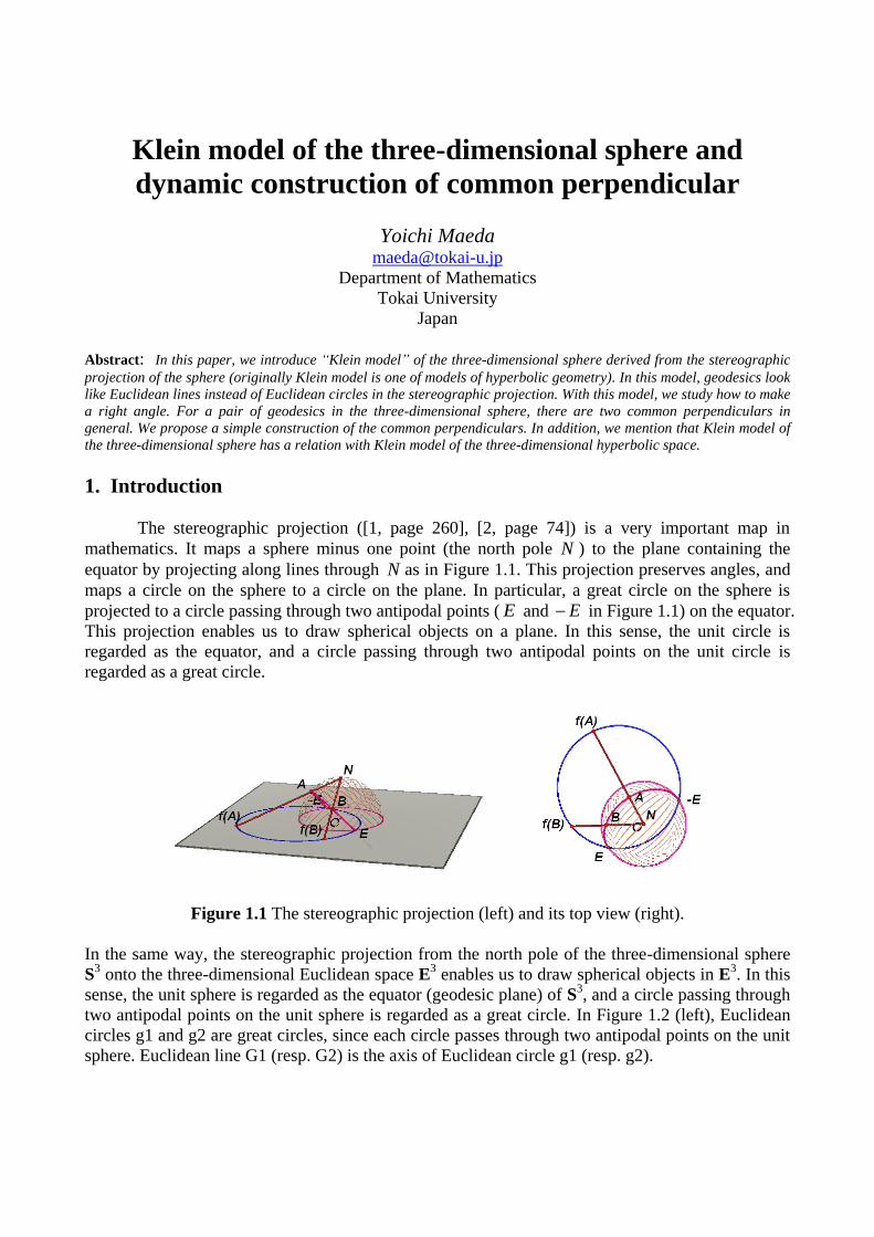
The stereographic projection ([1, page 260], [2, page 74]) is a very important map in

mathematics. It maps a sphere minus one point (the north pole N ) to the plane containing the

equator by projecting along lines through N as in Figure 1.1. This projection preserves angles, and

maps a circle on the sphere to a circle on the plane. In particular, a great circle on the sphere is

projected to a circle passing through two antipodal points ( E and E in Figure 1.1) on the equator.

This projection enables us to draw spherical objects on a plane. In this sense, the unit circle is

regarded as the equator, and a circle passing through two antipodal points on the unit circle is

regarded as a great circle.

Figure 1.1 The stereographic projection (left) and its top view (right).

In the same way, the stereographic projection from the north pole of the three-dimensional sphere

S3 onto the three-dimensional Euclidean space E

3 enables us to draw spherical objects in E

3. In this

sense, the unit sphere is regarded as the equator (geodesic plane) of S3, and a circle passing through

two antipodal points on the unit sphere is regarded as a great circle. In Figure 1.2 (left), Euclidean

circles g1 and g2 are great circles, since each circle passes through two antipodal points on the unit

sphere. Euclidean line G1 (resp. G2) is the axis of Euclidean circle g1 (resp. g2).

Figure 1.2 Stereographic projection (left) and Klein model (right).

There is a one-to-one correspondence between a great circle and its axis. In this paper, let us

propose “Klein” model in which we regard Euclidean lines G1 and G2 as the geodesics of the three

dimensional sphere as in Figure 1.2 (right). The following construction shows how to draw the

corresponding great circle g in the stereographic projection from a geodesic G in the Klein model.

Construction 1.1 (great circle g in stereographic projection from geodesic G in Klein model)

0. (Input) Euclidean line G.

1. Plane containing G and O (center of the unit sphere).

2. Line L perpendicular to through O.

3. Points E and –E, intersections of L and the unit sphere.

4. (Output) Euclidean circle g around G through E or –E.

Note that if g is a Euclidean line through O, then G is a line at infinity. Hence Klein model is

realized in three-dimensional projective space P3. One of the merits of this model is that it is easy to

make a right angle. To do this, we need conjugate geodesic. In Section 2, we will see the

construction of the conjugate geodesic. With conjugate geodesic, we will consider the construction

of the common perpendicular. In [3], we have already seen a dynamic construction of the common

perpendicular. In Section 3, we will introduce a simpler construction with the same idea. In

addition, we will see that the Klein model of the three-dimensional sphere has a close relation with

the Klein model of the three-dimensional hyperbolic space H3 in Section 4. All pictures in this

paper are created by dynamic geometry software Cabri II plus and Cabri 3D.

2. Conjugate Geodesic 2.1. Two intersecting geodesics

Figure 2.1 Two intersecting geodesics.

If two great circles g1 and g2 intersect, then these two great circles are contained in a great

sphere g1∪g2. The sphere g1∪g2 is centered at the intersection G1∩G2 of axes G1 and G2,

containing the great circle on the unit sphere passing through two pairs of antipodal points on g1

and g2 as in Figure 2.1. Hence g1 and g2 intersect in the stereographic projection, if and only if, G1

and G2 intersect in the Klein model. The next step is to create a right angle in this model. To do this,

we have to prepare the farthest geodesic called “conjugate geodesic”.

2.2. Conjugate geodesic

Figure 2.2 Conjugate geodesic in the stereographic projection.

Figure 2.2 is the stereographic projection of S3. For a great circle h (Euclidean line), h⊥ is far

from h with 90 degrees. h⊥ is the set of the farthest points from h which is called “conjugate

geodesic”. (Note that any great sphere containing h intersects with h⊥at a right angle, vice versa.)

In Figure 2.2, g is a great circle which intersects with h and also with h⊥. Then g intersects with h

at a right angle, and also g intersects with h⊥ at a right angle. This picture indicates how to make

right angle in the Klein model, i.e., if G intersects with H and H⊥, then G⊥H and G⊥H⊥. Now let

us see the construction of conjugate geodesic G⊥ from G in Figure 2.3.

Figure 2.3 Conjugate geodesic in Klein model.

Construction 2.1 (conjugate geodesic in Klein model)

0. (Input) Euclidean line G.

1. Point P1, intersection of G and the perpendicular plane from O to G.

2. Point P2, central symmetry of P1 through O.

3. Point P3, inversion with respect to the unit sphere.

4. (Output) Euclidean line G⊥ through P3 perpendicular to G.

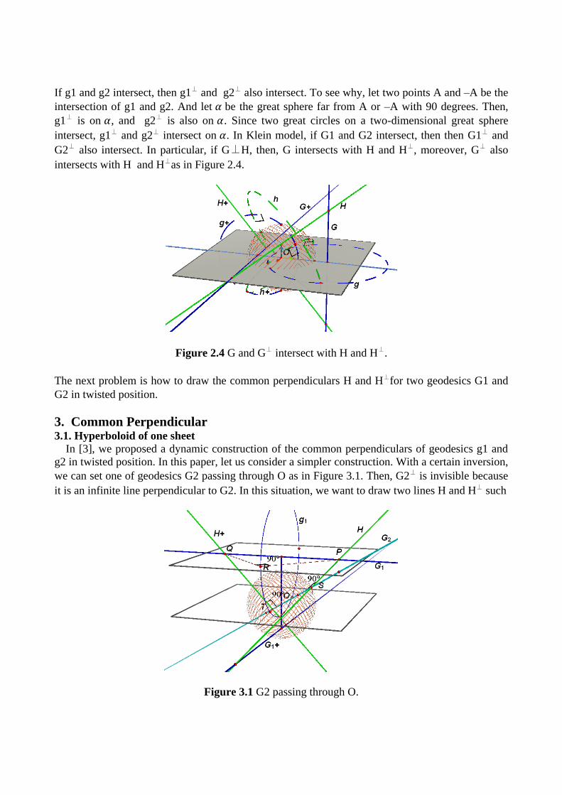
If g1 and g2 intersect, then g1⊥ and g2⊥ also intersect. To see why, let two points A and –A be the

intersection of g1 and g2. And let be the great sphere far from A or –A with 90 degrees. Then,

g1⊥ is on , and g2⊥ is also on . Since two great circles on a two-dimensional great sphere

intersect, g1⊥ and g2⊥ intersect on . In Klein model, if G1 and G2 intersect, then then G1⊥ and

G2⊥ also intersect. In particular, if G⊥H, then, G intersects with H and H⊥, moreover, G⊥ also

intersects with H and H⊥as in Figure 2.4.

Figure 2.4 G and G⊥ intersect with H and H⊥.

The next problem is how to draw the common perpendiculars H and H⊥for two geodesics G1 and

G2 in twisted position.

3. Common Perpendicular 3.1. Hyperboloid of one sheet In [3], we proposed a dynamic construction of the common perpendiculars of geodesics g1 and

g2 in twisted position. In this paper, let us consider a simpler construction. With a certain inversion,

we can set one of geodesics G2 passing through O as in Figure 3.1. Then, G2⊥ is invisible because

it is an infinite line perpendicular to G2. In this situation, we want to draw two lines H and H⊥ such

Figure 3.1 G2 passing through O.

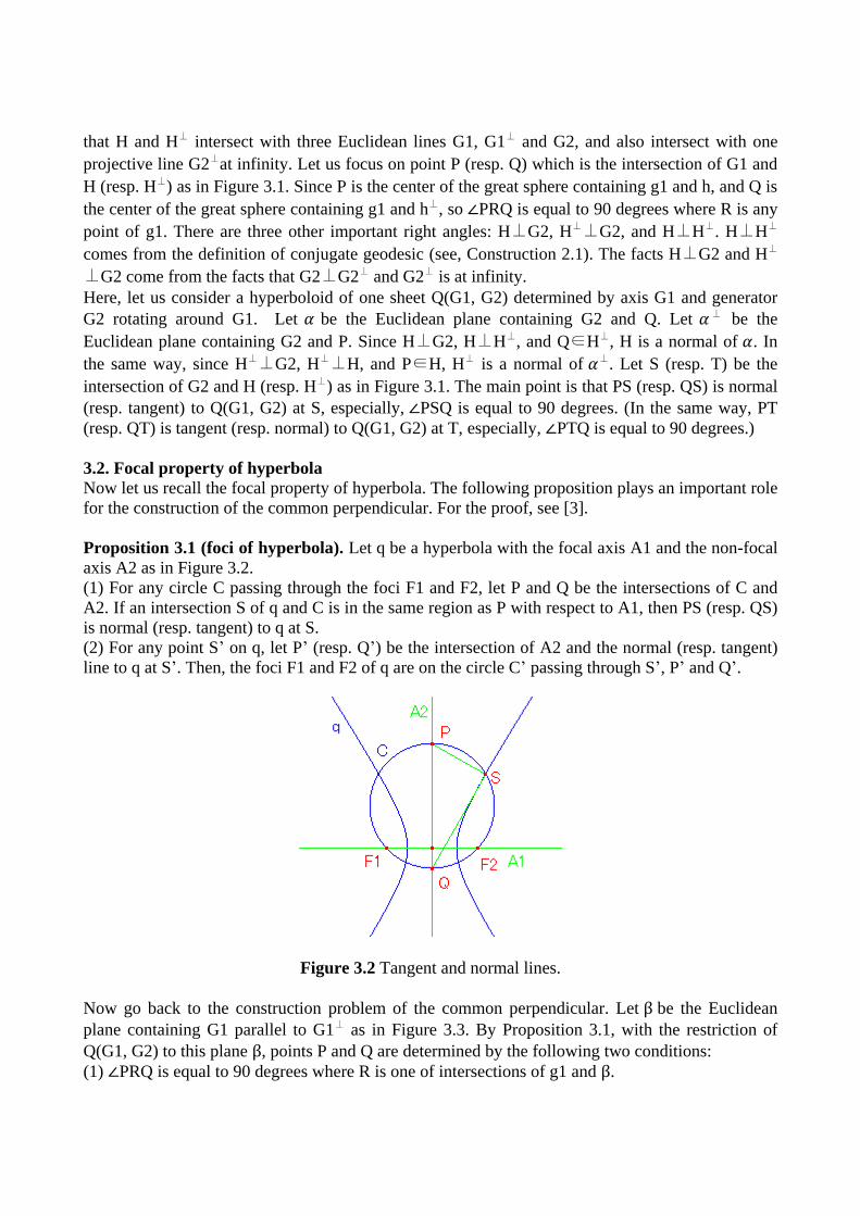
that H and H⊥ intersect with three Euclidean lines G1, G1⊥ and G2, and also intersect with one

projective line G2⊥at infinity. Let us focus on point P (resp. Q) which is the intersection of G1 and

H (resp. H⊥) as in Figure 3.1. Since P is the center of the great sphere containing g1 and h, and Q is

the center of the great sphere containing g1 and h⊥, so PRQ is equal to 90 degrees where R is any

point of g1. There are three other important right angles: H⊥G2, H⊥⊥G2, and H⊥H⊥. H⊥H⊥

comes from the definition of conjugate geodesic (see, Construction 2.1). The facts H⊥G2 and H⊥

⊥G2 come from the facts that G2⊥G2⊥ and G2⊥ is at infinity.

Here, let us consider a hyperboloid of one sheet Q(G1, G2) determined by axis G1 and generator

G2 rotating around G1. Let be the Euclidean plane containing G2 and Q. Let ⊥ be the

Euclidean plane containing G2 and P. Since H⊥G2, H⊥H⊥, and Q∈H⊥, H is a normal of . In

the same way, since H⊥⊥G2, H⊥⊥H, and P∈H, H⊥ is a normal of ⊥. Let S (resp. T) be the

intersection of G2 and H (resp. H⊥) as in Figure 3.1. The main point is that PS (resp. QS) is normal

(resp. tangent) to Q(G1, G2) at S, especially, PSQ is equal to 90 degrees. (In the same way, PT

(resp. QT) is tangent (resp. normal) to Q(G1, G2) at T, especially, PTQ is equal to 90 degrees.)

3.2. Focal property of hyperbola Now let us recall the focal property of hyperbola. The following proposition plays an important role

for the construction of the common perpendicular. For the proof, see [3].

Proposition 3.1 (foci of hyperbola). Let q be a hyperbola with the focal axis A1 and the non-focal

axis A2 as in Figure 3.2.

(1) For any circle C passing through the foci F1 and F2, let P and Q be the intersections of C and

A2. If an intersection S of q and C is in the same region as P with respect to A1, then PS (resp. QS)

is normal (resp. tangent) to q at S.

(2) For any point S’ on q, let P’ (resp. Q’) be the intersection of A2 and the normal (resp. tangent)

line to q at S’. Then, the foci F1 and F2 of q are on the circle C’ passing through S’, P’ and Q’.

Figure 3.2 Tangent and normal lines.

Now go back to the construction problem of the common perpendicular. Let be the Euclidean

plane containing G1 parallel to G1⊥ as in Figure 3.3. By Proposition 3.1, with the restriction of

Q(G1, G2) to this plane , points P and Q are determined by the following two conditions:

(1) PRQ is equal to 90 degrees where R is one of intersections of g1 and .

(2) PFQ is equal to 90 degrees where F is one of the foci of the hyperbola q(G1, G2) which is the

intersection of Q(G1, G2) and .

Figure 3.3 Hyperbola on the plane (left) and its top view (right).

Consequently, P and Q is the intersection of G1 and the circle passing through R, F1 and F2 as in

Figure 3.3. To find out the foci F1 and F2, we use the fact that G2 looks like a tangent of q(G1, G2)

at the intersection of G2 and as in Figure 3.3 (right).

3.3. Construction of the common perpendiculars Now let us propose a simple construction of the common perpendiculars as in Figure 3.4. The

former half of the following construction is to find out the foci of q(G1, G2).

Figure 3.4 The Construction of the common perpendiculars.

Construction 3.1 (common perpendiculars in the Klein model)

0. (Input) Three geodesics, G1, G1⊥, and G2 (G2 passes through O).

1. Plane containing G1 parallel to G1⊥.

2. Point P1, intersection of and G2.

3. Point P2, half turn of P1 around G1.

4. Point P3 on G1, pedal of the common perpendicular of G1 and G1⊥.

5. Circle C1 passing through P1, P2 and P3.

6. Point P4 on G1, pedal of the common perpendicular of G1 and G2 (center of q(G1, G2)).

7. Line L1 on perpendicular to G1 through P4.

8. Points F1 and F2, intersection of C and L1 (foci of q(G1, G2)).

9. Points P5 and P6, intersection of g1 and .

10. Circle C2 passing through F1, F2, P5, and P6.

11. Points P and Q, intersection of C2 and G1.

12. (Output) Lines H and H⊥, perpendicular lines to G2 through P and Q, respectively.

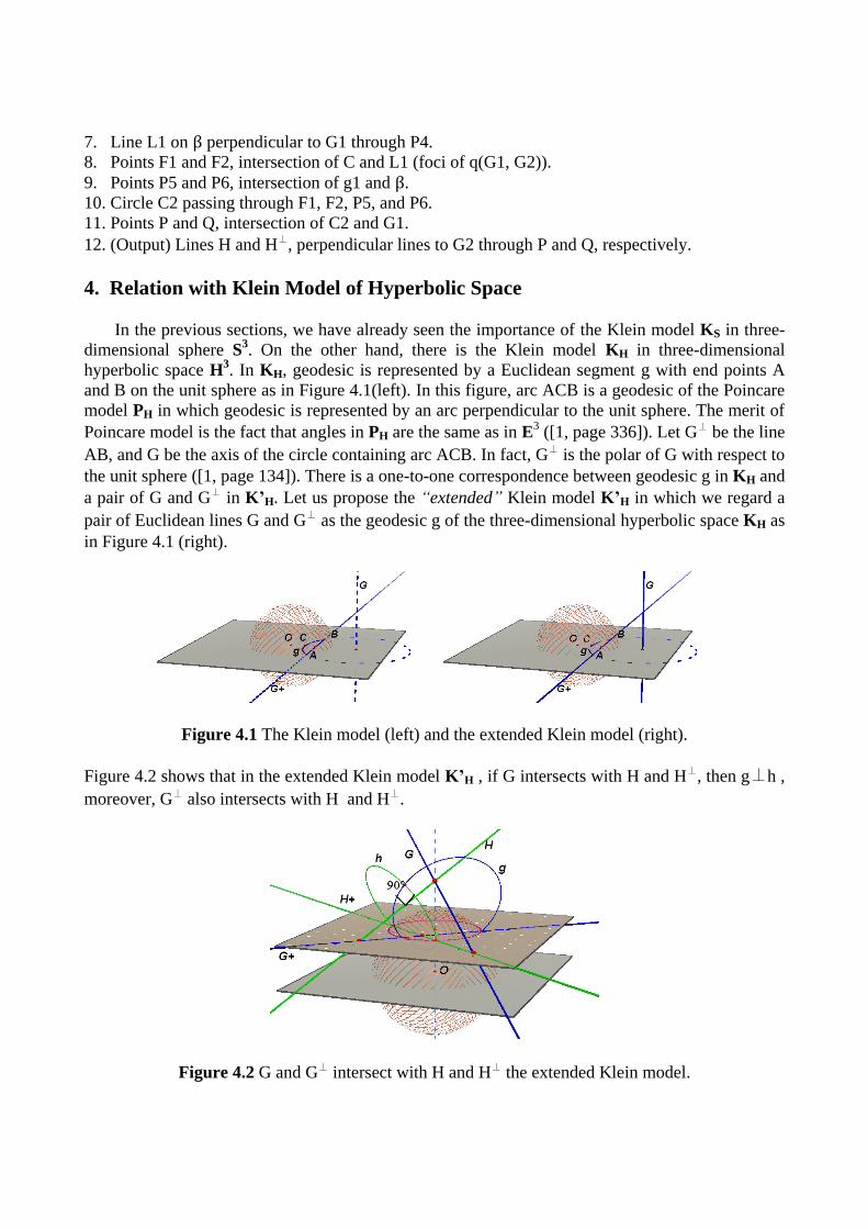
4. Relation with Klein Model of Hyperbolic Space

In the previous sections, we have already seen the importance of the Klein model KS in three-

dimensional sphere S3. On the other hand, there is the Klein model KH in three-dimensional

hyperbolic space H3. In KH, geodesic is represented by a Euclidean segment g with end points A

and B on the unit sphere as in Figure 4.1(left). In this figure, arc ACB is a geodesic of the Poincare

model PH in which geodesic is represented by an arc perpendicular to the unit sphere. The merit of

Poincare model is the fact that angles in PH are the same as in E3 ([1, page 336]). Let G⊥ be the line

AB, and G be the axis of the circle containing arc ACB. In fact, G⊥ is the polar of G with respect to

the unit sphere ([1, page 134]). There is a one-to-one correspondence between geodesic g in KH and

a pair of G and G⊥ in K’H. Let us propose the “extended” Klein model K’H in which we regard a

pair of Euclidean lines G and G⊥ as the geodesic g of the three-dimensional hyperbolic space KH as

in Figure 4.1 (right).

Figure 4.1 The Klein model (left) and the extended Klein model (right).

Figure 4.2 shows that in the extended Klein model K’H , if G intersects with H and H⊥, then g⊥h ,

moreover, G⊥ also intersects with H and H⊥.

Figure 4.2 G and G⊥ intersect with H and H⊥ the extended Klein model.

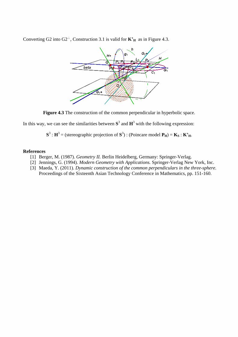
Converting G2 into G2⊥, Construction 3.1 is valid for K’H as in Figure 4.3.

Figure 4.3 The construction of the common perpendicular in hyperbolic space.

In this way, we can see the similarities between S3 and H

3 with the following expression:

S3 : H

3 = (stereographic projection of S

3) : (Poincare model PH) = KS : K’H.

References

[1] Berger, M. (1987). Geometry II. Berlin Heidelberg, Germany: Springer-Verlag.

[2] Jennings, G. (1994). Modern Geometry with Applications. Springer-Verlag New York, Inc.

[3] Maeda, Y. (2011). Dynamic construction of the common perpendiculars in the three-sphere.

Proceedings of the Sixteenth Asian Technology Conference in Mathematics, pp. 151-160.