Keynesian 01

8/10/2019 Keynesian 01

http://slidepdf.com/reader/full/keynesian-01 1/50

Keynesian System I : Role of Aggregate Demand

• The Problem of Unemployment: The Keynesian Economics

was developed against the background of the great

depression of 1930s.• The effect of depression on the US economy: unemployment

increases from 3.2% in 1929 to 25.2% in 1933.

• Real GNP decreased by 30%

• According to JM Keynes, high unemployment in GB and USand other economies was due to deficiency in aggregate

demand.

• Aggregate demand was low due to low investment demand.

• Keynes says, to remove unemployment, aggregate demandhas to increase, which need fiscal policy and govt. in the

form of spending on public work project.

Copyright © Dorling Kindersley India Pvt. Ltd.1






Keynesian System I : Role of Aggregate Demand

• Central notion in keynesian model in achieving an

equilibrium level of output requires, Output = Aggregate

demand.

• Aggregate demand = E = C + I + G

• C = HH consumption

• I = Desired business investment

• G = govt. sector demand for goods and services.

• GDP = GNP (closed economy)

• GDP = NDP (depreciation ignored)

• Aggregate price level is fixed

• Y = national income = C + S + T

• Income is either consumed, saved or paid out as taxes.




• Y = national product = C + Ir + G

• Ir = realised investment

• G = govt spending

• C = consumption

•Income = Expenditure

• C + S + T = Y = C + I + G

• S + T = I + G

• Product = Expenditure

• C + Ir + G = C + I + G• So, Ir = I




• So, the condtion for equilibrium in the model is• Y = C + I + G (1)

• S + T = I + G (2)

• Ir = I (3)










The Components of Aggregate Demand

• Consumption(C):

• Kenes Psychological law of consumption statesthat Consumer expenditure was a stable

function of disposable income.

• C = bYd

----- (4)

• Where, a>0 and 0< b <1

• b is the slope of the consumption function,

measures the increase in consumption due to

per unit increase in the disposable income;

• b = MPC = C/ Yd












The Components of Aggregate Demand

• Investment(I): Changes in the desired business

investment expenditure is one of the majorfactor that keynes thought responsible for

changes in income.

• Investment primarily responsible for instability

of income.

• Investment is determined by (i) interest rate

and (ii) business expectations.

• Govt. expenditures(G):are controlled by the

policy makers.




Determining the Equilibrium Level of Income

• E = Y = C + I + G

• Where, C = a + bYd = a + by – bT• (as Yd = Y – T)

• Y = a + bY – bT + I + G

• Or, Y – bY = a – bT + I + G

• Y (1 – b) = a – bT + I + G

• Or Y = 1 / (1 – b) [a – bT + I + G] ----------(5)







Determining the Equilibrium Level of Income

• Horizontal axis represents – Income

• Vertical axis represents – aggregate expenditure• 45 0 line indicates the all the points along this line,

aggregate income = aggregate expenditure

• E = Y = C + I + G

• We derive the aggregate expenditure (E) by adding I +G to C = a + bYd at each level of income.

• Because autonomous expenditure component does not

depend on the income and C + I + G curve lies above

the consumption function by a constant amount.






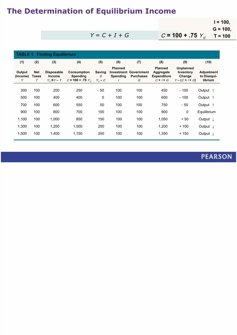
Y = C + I + G

TABLE 1 Finding Equilibrium

(1) (2) (3) (4) (5) (6) (7) (8) (9) (10)

Output

(Income)

Y

Net

Taxes

T

Disposable

Income

Y d ≡Y T

Consumption

Spending

C = 100 + .75 Y d

Saving

S

Y d – C

Planned

Investment

Spending

I

Government

Purchases

G

Planned

Aggregate

Expenditure

C + I + G

Unplanned

Inventory

Change

Y (C + I + G )

Adjustment

to Disequi-

librium

300 100 200 250 - 50 100 100 450 - 150 Output ↑

500 100 400 400 0 100 100 600 - 100 Output ↑

700 100 600 550 50 100 100 750 - 50 Output ↑

900 100 800 700 100 100 100 900 0 Equilibrium

1,100 100 1,000 850 150 100 100 1,050 + 50 Output ↓

1,300 100 1,200 1,000 200 100 100 1,200 + 100 Output ↓

1,500 100 1,400 1,150 250 100 100 1,350 + 150 Output ↓

The Determination of Equilibrium Income

C = 100 + .75 Y d

I = 100,

G = 100,

T = 100

D t i i th E ilib i L l f I



Determining the Equilibrium Level of Inco

• From the equation of determining the equilibrium

level of income, we have derived the E = a + bY – bT+ I + G

• In the above equation, the component a – bT + I + G

represents the autonomous components of

expenditure.

• The expenditure function shift every time these

expenditure components change.

• The slope of the expenditure function is thecoefficient of Y i.e. b (MPC)




Determining the Equilibrium Level ofIncome

• So, when the MPC decreases, theexpenditure function is flatter and when

MPC increases, the expenditure function is

steeper.• YE = (autonomous exp. Multiplier) x

(autonomous expenditure)

• YE = 1 / (1-b) [a – bT + G + I)





• The expenditure multiplier = k• The marginal propensity to consume = b

• So, when b = 0.5 k = 2

b = 0.8 k = 5b = 0.9 k = 10

The autonomous expenditure multiplier gives the

changes in the equilibrium level of output perunit change in the autonomous expenditure





•The autonomous expenditure are the expenditure that arelargely determined by factors other than current income.

• a = autonomous component of consumption expenditure

• bT = autonomous affect of tax collection on aggregate

demand and determined through marginal propensityto consume.

• (a – bT) determines the height of the consumption

function.

• I = autonomous investment• G = autonomous govt. expenditure




The Investment Multiplier



MPS S

Y

MPS I

Y

Because S must be equal to I for equilibrium to be restored, wecan substitute I for S and solve:

Therefore, Y I MPS

1

, or

Recall that the marginal propensity to save (MPS)is the fraction of a change in income that is

saved. It is defined as the change in S (∆S) overthe change in income (∆Y ):

The Investment Multiplier

MPS 1multiplier

MPC - 11multiplier It followsthat






TABLE 2 Finding Equilibrium after a Investment Increase of 50 (I Has Increased from 100 in Table 1

to 150 Here)

(1) (2) (3) (4) (5) (6) (7) (8) (9) (10)

Output

(Income)

Y

Net

Taxes

T

Disposable

Income

Y d ≡Y T

Consumption

Spending

C = 100 + .75 Y d

Saving

S

Y d – C

Planned

Investment

Spending

I

Government

Purchases

G

Planned

Aggregate

Expenditure

C + I + G

Unplanned

Inventory

Change

Y (C + I + G )

Adjustment

to

Disequilibrium

300 100 200 250 - 50 150 100 500 - 200 Output ↑

500 100 400 400 0 150 100 650 - 150 Output ↑

700 100 600 550 50 150 100 800 - 100 Output ↑

900 100 800 700 100 150 100 950 - 50 Output ↑

1,100 100 1,000 850 150 150 100 1,100 0 Equilibrium

1,300 100 1,200 1,000 200 150 100 1,250 + 50 Output ↓

Fiscal Policy at Work: Multiplier Effects





TABLE 24.2 Finding Equilibrium after a Government Spending Increase of 50 (G Has Increased from

100 in Table 9.1 to 150 Here)

(1) (2) (3) (4) (5) (6) (7) (8) (9) (10)

Output

(Income)

Y

Net

Taxes

T

Disposable

Income

Y d ≡Y T

Consumption

Spending

C = 100 + .75 Y d

Saving

S

Y d – C

Planned

Investment

Spending

I

Government

Purchases

G

Planned

Aggregate

Expenditure

C + I + G

Unplanned

Inventory

Change

Y (C + I + G )

Adjustment

to

Disequilibrium

300 100 200 250 - 50 100 150 500 - 200 Output ↑

500 100 400 400 0 100 150 650 - 150 Output ↑

700 100 600 550 50 100 150 800 - 100 Output ↑

900 100 800 700 100 100 150 950 - 50 Output ↑

1,100 100 1,000 850 150 100 150 1,100 0 Equilibrium

1,300 100 1,200 1,000 200 100 150 1,250 + 50 Output ↓


The Government Spending Multiplier



Increasing governmentspending by 50 shifts the

AE function up by 50.As Y rises in response,additional consumption is

generated.Overall, the equilibriumlevel of Y increases by200, from 900 to 1,100.

The Government Spending Multiplier



tax multiplier The ratio of change in the equilibrium level ofoutput to a change in taxes.

tax multiplier MPC

MPS

-

Y MPS

(initial increase in aggregate expenditure) 1

1( ) MPC Y T MPC T

MPS MPS - -

The Tax Multiplier

Because the initial change in aggregate expenditure caused by atax change of ∆T is (−∆T × MPC ), we can solve for the taxmultiplier by substitution:

Because a tax cut will cause an increase in consumptionexpenditures and output and a tax increase will cause a reduction in consumption expenditures and output, the tax multiplier is a

negative multiplier:










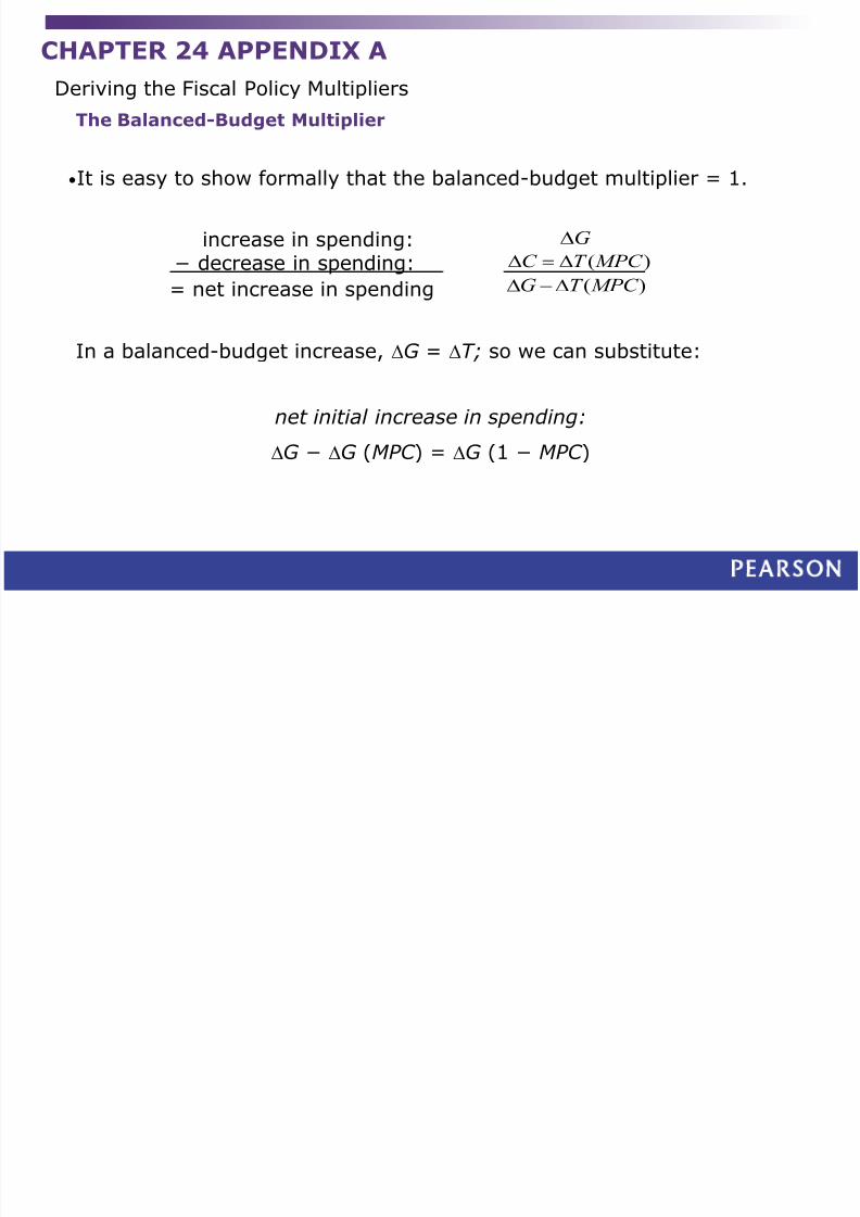
•It is easy to show formally that the balanced-budget multiplier = 1.

Gincrease in spending:( )C T MPC − decrease in spending:

( )G T MPC - = net increase in spending

In a balanced-budget increase, G = T; so we can substitute:

net initial increase in spending:

G −

G (MPC ) =

G (1 − MPC )

Deriving the Fiscal Policy Multipliers

The Balanced-Budget Multiplier



1( )Y G MPS G

MPS

Because MPS = (1 − MPC ), the net initial increase in spending is:

G (MPS)

We can now apply the expenditure multiplier to this net initialincrease in spending:

MPS

1



Thus, the final total increase in the equilibrium level of Y is just equalto the initial balanced increase in G and T .




TABLE 3 Finding Equilibrium after a Balanced-Budget Increase in G and T of 200 Each (Both G and

T Have Increased from 100 in Table 1 to 300 Here)

(1) (2) (3) (4) (5) (6) (7) (8) (9)

Output

(Income)

Y

Net

Taxes

T

Disposable

Income

Y d ≡Y T

Consumption

Spending

C = 100 + .75 Y d

Planned

Investment

Spending

I

Government

Purchases

G

Planned

Aggregate

Expenditure

C + I + G

Unplanned

Inventory

Change

Y (C + I + G )

Adjustment

to

Disequilibrium

500 300 200 250 100 300 650- 150 Output ↑

700 300 400 400 100 300 800 - 100 Output ↑

900 300 600 550 100 300 950 - 50 Output ↑

1,100 300 800 700 100 300 1,100 0 Equilibrium

1,300 300 1,000 850 100 300 1,250 + 50 Output ↓

1,500 300 1,200 1,000 100 300 1,400 + 100 Output ↓






TABLE 4 Summary of Fiscal Policy Multipliers

Policy Stimulus Multiplier

Final Impact on

Equilibrium Y

Government

spending

multiplier

Increase or decrease in the

level of government

purchases: ∆G

Tax multiplier Increase or decrease in the

level of net taxes: ∆T

Balanced-budget

multiplier

Simultaneous balanced-budget

increase or decrease in thelevel of government purchases

and net taxes: ∆G = ∆T

1

1

MPS

- MPC

MPS

1 G

MPS

MPC

T MPS

-

G





The Federal Budget



federal budget The budget of the federalgovernment.

The “budget” is really three different budgets:

It is a political document that dispenses favors to certain groups or regionsand places burdens on others.

It is a reflection of goals the government wants to achieve.

The budget may be an embodiment of some beliefs about how (if at all)the government should manage the macroeconomy.

The Federal Budget

The Federal Budget



TABLE 24.5 Federal Government Receipts and Expenditures, 2009 (Billions of Dollars)

Amount Percentage of Total

Current receipts

Personal income taxes 828.7 37.2

Excise taxes and customs duties 92.3 4.1

Corporate income taxes 231.0 10.4

Taxes from the rest of the world 12.3 0.6

Contributions for social insurance 949.1 42.7

Interest receipts and rents and royalties 48.2 2.2Current transfer receipts from business and persons 68.1 3.1

Current surplus of government enterprises − 4.9 − 0.2

Total 2,224.9 100.0

Current Expenditures

Consumption expenditures 986.4 28.6

Transfer payments to persons 1596.1 46.2

Transfer payments to the rest of the world 61.7 1.8

Grants-in-aid to state and local governments 476.6 13.8

Interest payments 272.3 7.9

Subsidies 58.2 1.7

Total 3,451.3 100.0

Net federal government saving—surplus (+) or deficit (−)

(Total current receipts − Total current expenditures) − 1,226.4

The Federal Budget

The Budget in 2009

The Federal Budget



federal surplus (+) or deficit (−) Federal government receiptsminus expenditures.

The Federal Budget

The Budget in 2009

CHAPTER 24 APPENDIX A



Y C I G

C a b Y T -( )

Y a b Y T I G - ( )

Y a bY bT I G -

Y bY a I G bT - -

Y b a I G bT ( )1- -

)(

1

1bT G I a

b Y -

-


The Government Spending and Tax Multipliers

We can derive the multiplier algebraically using our hypotheticalconsumption function:

The equilibrium condition is

By substituting for C , we get

This equation can be rearranged to yield

Now solve for Y by dividing through by (1 − b):

CHAPTER 24 APPENDIX A



•It is easy to show formally that the balanced-budget multiplier = 1.

Gincrease in spending:( )C T MPC − decrease in spending:

( )G T MPC - = net increase in spending

In a balanced-budget increase, G = T; so we can substitute:

net initial increase in spending:

G − G (MPC ) = G (1 − MPC )





CHAPTER 24 APPENDIX B



T Y Y d

-

)3/1200( Y Y Y d --

Y Y Y d

3/1200 -

d Y C 75.100

)3/1200(75.100 Y Y C -

FIGURE 24B.1 The Tax Function

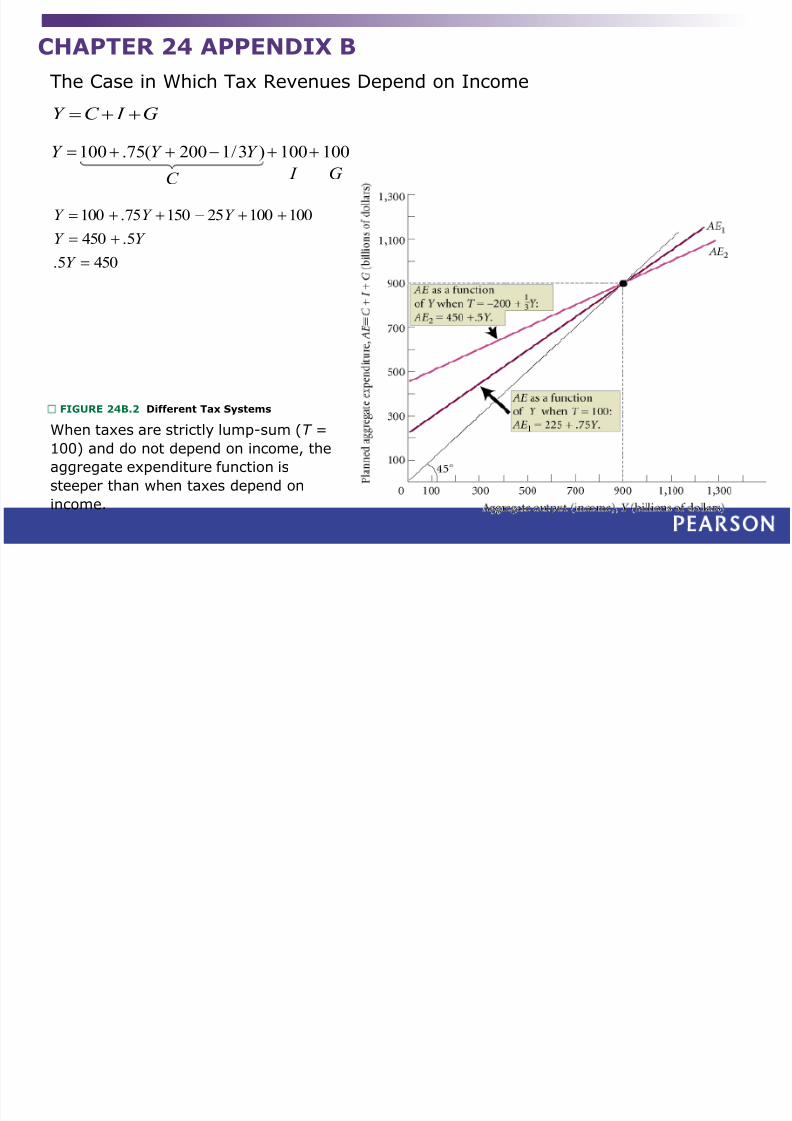
The Case in Which Tax Revenues Depend on Income

This graph shows net taxes

(taxes minus transfer payments)as a function of aggregateincome.




When taxes are strictly lump-sum (T =100) and do not depend on income, the

aggregate expenditure function is

steeper than when taxes depend on

income.

FIGURE 24B.2 Different Tax Systems

G I C Y

100 .75( 200 1/3 ) 100 100Y Y Y I GC

-

4505.

5.450

1001002515075.100

-

Y

Y Y

Y Y Y

The Case in Which Tax Revenues Depend on Income




C a b Y T -( )

0C a bY bT btY - -

0( )C a b Y T tY - -

0Y a bY bT btY I G

C

- -

Y b bt

a I G bT -

-1

1 0( )

The Government Spending and Tax Multipliers Algebraically

The Case in Which Tax Revenues Depend on Incomes

Through substitution we get

Solving for Y :




1

1 b bt -

The Government Spending and Tax Multipliers Algebraically

The Case in Which Tax Revenues Depend on Incomes

This means that a $1 increase in G or I (holding a and T 0 constant) willincrease the equilibrium level of Y by

Holding a, I , and G constant, a fixed or lump-sum tax cut (a cut in T 0)will increase the equilibrium level of income by

bt b

b

-1






Documents

Keynesian 01