Embed Size (px)
Citation preview

PROGRESS REPORT : NOVEMBER 1990 ■ JUNE 1991
KENYA - BELGIUM PROJECT IN MARINE SCIENCES "HIGHER INSTITUTE FOR MARINE SCIENCES"
VLIR - KMFRI PROJECT
&CEC PROJECT
"DYNAMICS AND ASSESSMENT OF KENYAN MANGROVE ECOSYSTEMS"
no TS2-0240-C (GDF)
COMPILED BY Dr. K. DELBEKE
NOT TO BE CITED WITHOUT PRIOR AUTHORIZATION FROM THE AUTHORS

PROGRESS REPORT : NOVEMBER 1990 - JUNE 1991
KENYA - BELGIUM PROJECT IN MARINE SCIENCES "HIGHER INSTITUTE FOR MARINE SCIENCES"
VLIR - KMFRI PROJECT
&
CEC PROJECT "DYNAMICS AND ASSESSMENT OF KENYAN
MANGROVE ECOSYSTEMS" no TS2-0240-C (GDF)
COMPILED BY Dr. K. DELBEKE
NOT TO BE CITED WITHOUT PRIOR AUTHORIZATION FROM THE AUTHORS

KENYA-BELGIUM PROJECT IN MARINE SCIENCE VLIR - KMFRI PROJECT
P.O.Box 81651 Mombasa, Kenya
Tel. Fax : 254/11/742215
Director Kenya - Belgium Project : Prof. Dr. P. Polk Director KMFRI : Dr. E. Okemwa
Residential Manager : Dr. K. Delbeke
&
CEC PROJECT "DYNAMICS AND ASSESSMENT OF KENYAN
MANGROVE ECOSYSTEMS" n° TS2-0240-C (GDF)
Participating laboratories :
Kenya :K.M.F.R.I. (Dr. Okemwa)
Nairobi University : Dept. Zoology (Dr. Ntiba)
Belgium :V.U.B. - ANCH (Dr. Dehairs)
V.U.B. - ECOL (Dr. Daro)R.U.G. - Marine Biology (Dr. Vincx)
R.U.G. - Botany (Dr. Coppejans)
The Netherlands :Delta institute for Hydrobiological Research (Dr. Hemminga)
Catholic University Nijmegen : Aquatic Ecology (Prof. den Hertog)
Coordinating laboratory :V.U.B.- ECOL : Prof. Polk
Vrije Universiteit Brussel,Pleinlaan 2, B-1050 Brussels, Belgium.
i

Acknowledgements
We hereby thank the Kenyan and Belgium Governments for giving us the financial support and facilities to continue with the research project. We also thank the "Flemish Interuniversity Council" (VLIR) for their scientific support. We thank also the Commission of the European Communities, Directorate- General XII for their financial support. We are furthermore grateful to the Belgium Embassy and Cooperation in Nairobi and to the Belgian Consulate in Mombasa for their kind cooperation. We also thank SAREC and ROSTA, for their financial support in providing a scholarship for a researcher. Last but not least we are grateful to VVOB and to the Ministry of Science and Technology for their support by creating a link between KBP - KMFRI and VVOB.
2

TABLE OF CONTENTS1. INTRODUCTION 52. VISITING RESEARCHERS AND ORGANIZATIONS 63. SAMPLING DONE 94. RESULTS ON ONGOING RESEARCH 224.1. RESEARCH IN THE FRAME OF THE VLIR AND CEC PROJECT 22
4.1.1. Primary production in Mangroves, using biomass increments and litterfall.By : P.Gwada and E.Siim 22
4.1.2. Relative importance of mangrove litter as nutrient sourceBy : A.F.Woitchik, J.Kazungu, R.G.Rao and F.Dehairs 29
4.1.3. Nutrient dynamics in a tropical Mangrove Ecosystem (Gazi Creek).By : J.M.Kazungu 32
4.1.4. Species composition and primary production of Phytoplankton at Gazi Creek.By : P.Wawiye 37
4.1.5. Zooplankton studies in a Mangrove Creek System, Gazi.By : E.Okemwa, J.Mwaluma and M.Osore 40
4.1.6. Fundamental and Applied bacteriology in tropical marine waters.By : J.Wijnant, S.Mwangi and M.Owili 49
4.1.7. The fish community in a mangrove ecosystem.4.1.7.1. Fish community and fisheries studies of Gazi
Creek.By : E.O.Wakwabi in collaboration with M.Ntiba B.Okoth, G.Mwatha and E.Kimani 62
4.1.7.2. The fish community in Gazi Creek.By : M.Ntiba, E.O.Wakwabi, B.Okoth, E.Kimani, and G.Matha 67
4.1.8. Substrate influence on the physical and chemical properties of mangrove soils.By : K.K.Kairu 72
4.2. RESEARCH IN THE FRAME OF THE VLIR PROJECT 754.2.1. The distribution, growth and economic importance of the
Agarophyte, Gracilaria (Gigartinale) on the Kenya Coast.By :. H.A.Oyieke 75
4.2.2. Seeweeds of Kenya; a general survey of their economic potential along the Coast.By : J.G.Wakibia 81
4.2.3. A comparative Study of growth and recruitment of selected coral species along the Kenya Coast.By : J.Mutere 83
4.2.4. Assessment of pollution in the coastal and marine environment around Mombasa. 884.2.4.1. Theoretical Assessment of the pollution sources
and loads of the creeks around Mombasa.By : J.Munga, K.Delbeke.S.Tsalwa, S.Mwaguni and J.Wijnant 88
3

4.2.4.2. Monitoring of pollution levels in the coastal and estuarine environments around Mombasa.By : J.Wijnant, K.Delbeke.J.Munga, S.Mwangiand M.Owili 98
4.2.4.3. Assessment of pollution impact on the MangroveOyster, Crassostra cucullata. 106By : K.Delbeke.O.Omolo, M.Umani & O.Anyango
4.2.5. A report on the culture of Siganus sutor in tanks.By : B.Okoth 112
4.3. RESEARCH DONE BY VISITING SCIENTISTS 1135. OTHER ACTIVITIES 1646. CONCLUSION 1657. APPENDIX 166
4

1.INTRODUCTION
This report aims to give an overview of the results obtained over the last year in the frame of the VLIR project and the cooperating EEC project "Dynamics and Assessment of Kenyan Mangrove Ecosystems" (CEC Project nr TS 2-0240-C (GDF)).The Mangrove ecosystem in Gazi has been intensively investigated. The researchers of the different subproject are most often working in a coordinated way. A comprehensive set of data is now available and presented in this report.The Kenyan coastal area has especially been investigated for species distribution and coverage of marine algae and corals at different sites along the Kenyan coast.Most recently a pollution project, supported by UNEP, in collaboration with Kenyan Government chemist, was started. The first information on pollution sources and pollution loads have been obtained. The first data on monitoring of the pollution levels and their environmental impact, for the area around Mombasa are presented in this report.The aquaculture department is still small, nevertheless preliminary research is being done with success on fish culturing. The Oysters Commercial cultivation has started, is it on a very small scale. All information is now available to start real oyster farming.The Kenya - Belgium project was furthermore involved in the organization of a symposium: "Status and future of Large MarineEcosystems", to be held in between 2nd and 7th August 1992.
5
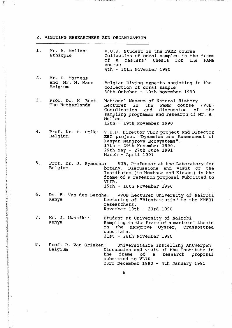
2. VISITING RESEARCHERS AND ORGANIZATION
Mr. A. Melles: Ethiopie
V .U .B . Student in the FAME course Collection of coral samples in the frame of a masters' thesis for the FAME course4th - 30th November 1990
Mr. D. Martens and Mr. M. Maes Belgium
Prof. Dr. M. Best The Netherlands
Prof. Dr. P. Polk: Belgium
Belgian Diving experts assisting in the collection of coral sample 30th October - 19th November 1990National Museum of Natural History Lecturer in the FAME course (VUB) Coordination and discussion of the sampling programme and research of Mr. A. Melles.12th - 19th November 1990V.U.B. Director VLIR project and Director EEC project "Dynamics and Assessment of Kenyan Mangrove Ecosystems".17th - 29th November 1990,29th May - 27th June 1991 March - April 1991
Prof. Dr. J. Symoensi VUB, Professor at the Laboratory for Belgium botany. Discussions and visit of the
Institutes (in Mombasa and Kisumu) in the frame of a research proposal submitted to VLIR.15th - 18th November 1'990
Dr. E. Van den Berghe: W O B Lecturer University of NairobiKenya Lecturing of "Biostatistis" to the KMFRI
researchers.November 19th - 23rd 1990
Mr. J. Mwaniki: Kenya
Student at University of Nairobi Sampling in the frame of a masters' thesis on the Mangrove Oyster, Crassostrea cucullata.21st - 28th November 1990
Prof. R. Van Grieken: Universitaire Instelling AntwerpenBelgium Discussion and visit of the Institute in
the frame of a research proposal submitted to VLIR23rd December 1990 - 4th January 1991
6

1 0 .
11.
12 .
13.
15.
16.
17.
Mrs. E. Burke: International center for OceanographicCanada Development (ICOD) - Canada
Discussion on possibilities for cooperation between KMFRI - VLIR and ICOD 24th February - 3rd March 1991
Mr. B. Demeulenaere: Belgium
M r . J . Tack : Belgium
V.U.B. Student in the FAME course Sampling in the frame of a masters' thesis on benthos, for the FAME course. 10th February - 9th March 1991V.U.B. PhD. student at the Laboratory for Ecology. Sampling in the frame of a PhD thesis on the Mangrove Oyster, Crassostrea cucullata.11th March - 31st March 1991
Mr. N. Dankers: Mr. D. Rjkeren Mr. 0. Klepper The Netherlands
Rijkssinstituut voor Naturbeheer (RIN) Netherlands.Discussion on possibilities for collaboration between KMFRI and RIN in the frame of coral reef management.13th March 1991
D r . I . Gordon : Kenya
Senior lecturer in Ecology - University of Nairobi. Exploratory visit in the frame of the research project on handedness of UCA.March 1991
Dr. T. Orekoya: Kenya
FAODiscussion and finalization of the UNEP programme "Assessment and Control of Pollution of the Kenyan Coastal and Marine Environment" . 2nd - 3rd April 1991
Mrs. A .F . Woitchick: V.U.B. Belgium representative ofBelgium EEC project
February - 4th March 1991 1st May - 27th July 1991
Mr. J. Githaiga: Kenya
PhD student at University of Nairobi. Sampling in the frame of a PhD programme on Mangrove Oysters 2nd - 3rd April 1991
7

18.
19.
20.
2 1 .
Dr. M. Ngoile : Tanzania
Director of Institute for Marine Sciences - Zanzibar Discussion on collaboration
with KMFRI13th - 19th May 1991
Dr. R. Getzinger: Mrs. A. Wilson Auerbacher USA
American Association for Advances in Sciences (AAAS) - USA
Discussion on possibilities for collaboration.18th May 1991
Dr. Z. Hussain: FAO mangrove ConsultantMr. G.M. Kinyanjui:Kenya Provincial Forest Officer - Kenya
Discussion, on management of Mangrove forest and p o s s i b i l i t i e s of collaboration. 21st May 1991
Mr. De Gregorio: FAO Agricultural division mappingItaly „consultant
FAO mapping consultant discussion of collaboration with EEC/ VLIR project 31st May 1991
8

3 . SAMPLING DONE
WORKPLAN: SAMPLING DONE IN THE MONTH OF NOVEMBER 1990
DATE TIDE DEP.TIHE AREA RES■OFFICER TRANSPORT ACTIVITY
Thu 1 HT : 15:07 8.00
Mon 5 LT:11:33 10.00
Makupa Kalru
KanamalKanamalKanamal
Oyleke Mutere Wakibya
Tub 6 LT:12:15 10.30 Vlplngo A.Melles
Thu 8 L T : 13:57 1 1.00 Nyalf WljnantLT : 13:57 10.00 N y a U Waklbya
t
Mon 12 HT : 12 : 57 11.00 Tudor Wynant
Tue 13 HT : 13 : 58 9.00 N.Coast Best et.al
Wed 14 LT: 08 : 37 8.00 KMFRI OmotoLT: 08:37 7.00 Gazi OhowaLT: 08 : 37 9.00 South
Coast Best et.al
Thu 15 HT : 15: 24 9.00 MaUndi Mutere &Best et.al
Car Coastal Erosion (VLIR)
Car Algae (VLIR)Corals (VLIR)Seaweed (KMFRI)
Car Corals (VLIR)
Car Bacteriology (VLIR)Car Seaweeds (VLIR)
Car/boat Bacteriology (VLIR)
Car/boat Corals (VLIR)
Sea urchin (KMFRI)Car N2 Fixation (EEC+VIIR)
Car/boat Corals (VLIR)
Car/boat Corals (VLIR)
Fr1 16 HT : 15 : 57 9.009.00
V1pingo Ma 11nd1
Oyleke Best et.al
CarCar
Marine Algae (VLIR) Corals (VLIR)
Sat 17 HT : 16:26
Sun 18 HT:16:52
Mon 19 to
Frl 23
18.00 Gazi Ntlba et.al. Car Fisheries (EEC)
15.00 Gazi Ntiba et.al. Car Fisheries (VLIR)
9.00 to 6.30 course statistics by Dr. Van den Berghe
Mon 26 HT : 18:55 15.00HT : 18: 55 9.00
Tue 27 HT:11:25 9.00
TudorSh1mon1
Gazi Gaz 1
WynantMwangl & Omondl
Shlmonl Waklbya
Wynant Waw1ye
carCar
Car
Bacteriology (VLIR)Art. & Sard. Fisheries (KMFR)Seaweed (KMFRI)
Bacteriology (VLIR/EEC) Phytoplankton (EEC/VLIR)
9

WORKPLAN: SAMPLING DONE IN THE MONTH OF DECEMBER 1990
PATE TIDE______ DEP.TIHE AREA________RES .OFFICER________TRANSPORT ACTIVITY
Mon
Tue
Wed
Fr1
HonThu
Fr I
Mon
Tue
Wed
Thu
Fri
3 HT : 16 : 58 12 . 0 0 Gaz 1 Gaz < Gaz 1
Kazungu Waw1ye W1Jnant
Car/boat Nutr1 ent/(EEC+VLIR)Phytoplankton/(EEC+VLIR) Bacter1ology/(EEC+VLIR)
4 HT:17.42 14.00 Gazi Okemwa et.alGazi Ngull & OnyangoGazi Sllm
Car/boat Zooplankton(EEC+VLIR) Hydrograpy(EEC) POM(EEC)
5 LT: 12. 11
LT:12. 11
7 LT : 13.02
10 HT : 10.03
13 HT : 14 . 19
14 HT : 15.05
9.00
9.00
11 . 0 0
9 . 00
9.00
9.00
Gazi Gaz 1 Gaz 1 Kwa le
VI pingo V 1 pingo
Tudor
Gaz 1 Gaz 1 Gaz 1
Gaz 1 Gaz 1
WakwablRuwaOhowaMunga et.al
Hutere Wak1bya
Wynant
Kazungu Waw1ye Wynant et.al
Okemwa et.aL Sl 1m
Car/boat F1sher1 es/(EEC+VLIR)Melobenthos(EEC)N2 F1xat1on(EEC+VLIR)
Car Pollution (VLIR)
Car Corals(VLIR)Seaweeds (VLIR)
Car/boat Bacteriology (VLIR)
Car/boat Nutr1ents(EEC+VLIR)Phytoplankton(EEC+VLIR) Bacter1ology(EEC+VLIR)
Car/boat Zooplankton(EEC+VLIR )POM (EEC)
L T : 8 . 5 7
17 LT : 10.36
18 LT : 11.01
19 LT : 11.34
8.00
8.00
10.00
Tudor
Kanamal
9.00 Mtwapa
K 1kambaI a T udo r
Munga et.al
Wak 1bya
Kazungu
Munga et.al Wakwabl
Car
Car
Car/boat
CarCar/boat
Pol lut 1 on(VLIR)
Seaweed (KMFRI)
Nutrients (VLIR)
• Pollution (VLIR) F‘ï sheri es (VLIR)
20 LT: 12.05 9.00 Gaz 1 Gaz 1 Gaz 1
WakwablRuwaOhowa
Car/boat Fisheries 'EEC+VLIR) Melobenthos (EEC)N2 Fixation (EEC+VLIR)
LT: 12.05
21 LT : 12.36
1 0 . 0 0
1 0 . 0 0
.Tudor
01an1/Msambwenl
Wynant
Munga et.al
Car/boat
Car/boat
Bacteriology (VLIR)
Pollution (VLIR)
LT: 12.36 10.00
D1an1
Mombasa
Waki bya
Klmanl Car
Seaweed (KMFRI)
Fish Biology (VLIR)
10

WORKPLAN: SAMPLING1 DONE IN THE MONTH OF JANUARY 1991
DATE TIDE DEP.TIME AREA RES.OFFICER TRANSPORT ACTIVITY
Mon 7 HT : 08 : 32 LT: 14 : 36
8.00 Tudor Wynant et at Car/boat Bacteriology (VLIR)
Tue 8 HT:09:21 LT:15:22
9.00 Gaz 1 Slim & Gwada Car Li tterfalI (EEC)
Thu 10 HT: 12: 19 LT:17:50
8.00 Gaz 1 Gaz 1
Okemwa et at Slim
Car/boat Zooplankton (EEC+VLIR) POM (EEC)
Fr1 11 HT : 13 : 54 LT: 07 : 49
Gaz 1 Gaz 1 Gaz 1
Kazungu Wawi yeWynant et at
Car/boat Nutrients (EEC+VLIR) Phytoplankton (EEC+VLIR) Bacteriology (EEC+VLIR)
Mon 14 HT:16:04 LT:09: 59
8.00 Tudor Wynant et at Car/boat Bacteriology (VLIR)
Tue 15 HT:16:34
LT: IO : 28
8.00
9 . 00
Mtwapa
Gaz 1
Mwacherla &KimaniSlim
Car/boatCar
Fisheries (KMFRI) Li tterfalI (EEC)
Wed 16 HT : 17 : 04 LT:10:57
Thu 17 HT:17:33 LT:11:23
8.008.30
Gaz i Tudor
SlimKazungu
Ca rCar/boat
Litterfall (EEC) Nutrients (VLIR)
Fri 18 HT:18:03 LT: 11: 50
9 .00 Gaz i Slim Car Litterfall (EEC)
Mon 2 1 HT:19:37 LT:13:16
8.00 Tudor Wynant et al Car Bacteriology (VLIR)
Tue 22 HT : 07 : 41 LT: 13:49
9.00 Gazi Gaz 1
Slim & Gwada Mwachirya & Kimani
Car/boat Litterfall (EEC)
Fisheries (KMFRI)
Thu 24 HT:08: 17 LT: 15 :12
14 .00 Tudor Mwatha Car/boat F1 sheries (VLIR)
Mon 28 HT : 15 : 22 LT :09: 10 ’
11 .00 Gazi Gaz 1 Gaz 1
Kazungu Wawi ye Wynant et al
Car/boat Nutrients (EEC+VLIR) Phytoplankton (EEC+VLIR) Bacteriology (EEC+VLIR)
11
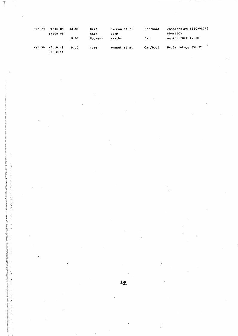
Tue 29 HT:16:09 13.00 Gazi Okemwa et al Car/boat Zooplankton (EEC+VLIR)LT :09:55 Gazi St1m POM(EEC)
9.00 Ngomenl Mwatha Car Aquaculture (VLIR)
Wed 30 HT:16:49 B.00 Tudor Wynant et al Car/boat Bacteriology (VLIR)LT:10:34
1*

WORKPLAN: SAMPLING SCHEOULE FOR THE MONTHS OF FEBRUARY & MARCH 1991
DATE TIDE
Fr1 1 LT : 11. 42
HT: 18.03
Sat 2 LT:12. 12 HT : 06 . 12
DEP.TIMË AREA
9.00 Gazi
Gazi Ha 11n d 1
Ma 11ndi
RES■OFFICER
Mwachlreya & K1man1 Omolo Kai ru
Ka 1 ru
TRANSPORT ACTIVITY
Car/boat F1sher1 es(KMFRI)
Echi noderms(KMFRI)Car Coastal erosion (VLIR)
Car Coastal eroslon(VLIR)
Mon 4 LT:13.16 11.00 Mtwapa OmoloHT:07.17 11.00 Tudor Omondi
Car Ech1noderms(KMFRI )Car/Boat Artisanal Fisheries
(KMFRI)
Tue 5 LT: 13.48 11.00 Gazi GwadaHT:07.48 Tudor Kazungu
Car/BoatCar/Boat
Litterfall (EEC) Nutrients (VLIR)
Wed 6 LT:14.22 13.00 Tudor Wynant et.al Car/BoatHT:08.23 12.00 Kanamal Waklbya Car
Bacter1ology(EEC/VLIR) Seaweed (EEC+VLIR)
Thu 7 LT: 15.01 14.00HT : 09.08
Fr 1 . 8 LT: 16.23 14.00HT: 10.38
Vipingo Oyleke Car Marine algae (VLIR)Vlplngo Omolo Echlnoderms (KMFRI)Gazi Wakwabl et.al. Car Fisheries (KMFRI)
KMFRI Omolo Car/Boat Echlnoderms (KMFRI)
Mon.11 LT: 09.15 13.00HT: 15.22
'' 9.15
Tue.12 LT: 09.46 13.00HT:15.52
8.00
Wed.13 LT : 10. 12 HT : 16. 13
8.00
9.009.0014.00
Gazi Gaz 1 Baha r1
Gaz 1 Gaz 1 Tudor
Gaz 1 Gaz i Gaz 1 Tudor Tudor K 1 1 1 n d 1 n1
WawiyeWynant et al Wak1bya
Osore Kazungu Omond i
Ka 1 ru Oy1 eke
Oe Meulenaere Wynant e I.al. Wynant Wakwabl
Car/Boat Phytoplankton (EEC +VLIR)Bacteriology (EEC+VLIR)
Car/boat Seaweed (VLIR)
Car/Boat Zooplankton (EEC+VLIR)Nutrients (EEC+VLIR)
Car/Boat Artisanat Fisheries (KMFRI)
Car/Boat Geology (EEC)Mar. Algae (VLIR)
Benthos (VLIR) Car/boat Bacteriology (VLIR)Car/Boat Bacteriology (VLIR)Car/boat Fisheries (VLIR)
Thu.14 L T : 10.37HT: 16.45
9.00 Fort Jesus OyiekeFort Jesus Omolo Engli shpointTudorTudor
De Meulenaere Wynant et.al. Wakwa^i
Car Marine algae (VLIR)Echinoderma (KMFRI)
Car/Boat , BenthosBacteriology (VLIR)
Car Fisheries (VLIR)
13

Fri . 15
Sun.17
Mon.18
Tue.19
Wed.20
Thu.21
Fr i . 22 4Sat. 23
Mon.25
Tue.26
Wed.27
Thu.28
Fr 1 , 1
LT:11.01 8.00 Port Reitz KairuHT: 17. 15 Ngomeni Wakibya
CarCar
Geology (VLIR) Seaweed (VLIR)
LT: 11.51 HT : 18. 10
9.00 Di ani Di ani
Ka i ru Omolo
Car Coastal erosion(VLIR) Echinoderma (KMFRI)
L T : 12.18 11.00HT: 18.38
1 1 . 00
LT:12.48 HT : 06.46
9.00
Tudor Tudor Di ani
Gaz 1
Gaz i Gazi
Wynant el.ol De Meulenaere Wak 1bya
Mwachi reya & Kimani GwadaDemeulenaere
Car/Boat Bacteriology (VLIR)Benthos (VLIR)
Car/boat Seaweed (VLIR)
Car/Boat Fisheries (KMFRI)Litterfall (EEC)
Benthos (VLIR)
11 . 00
LT: 13.13 11.00HT : 07. 19
1 0 . 0 0
LT: 13.54 11.00HT : 07.5 5 10.00
Tudor
KilifiKilifiShimoni
Kanama i Mambru i
Omond1 Kazungu
Oy i eke Omolo Waki bya
Omolo Wak 1bya
Car/Boat Art.Fisheries (KMFRI) Nutrients(VLIR)
Car Marine algae (VLIR)Echlnoderms (KMFRI)
Car/boat Seaweed (VLIR)
Car Echlnoderms (KMFRI)Car Seaweed (VLIR)
LT: 14.36 11.00 MalindiHT : 08.43 Lamu
Omolo Car Echlnoderms (KMFRI)
LT: 08.08 9.00HT:14.23 .
8.00
LT: 09.0 1 13.00HT: 15.15
GaziGazi
Tudor
Gaz i Gazi
Wawi yeWynant et. al.
Omond1
OsoreKazungu
Car/Boat Phytoplankton (EEC+VLIR)Bacteriology (EEC+VLIR)
Car/Boat Art. Fisheries (KMFRI)
Car/Boat Zooplanton (EEC+VLIR)Nutrients (EEC+VLIR)
LT : 09.42 HT: 15.56
LT:10. 16 HT:16.33
8.00
9.00
8.00
TudorTudorFloridaclub
L i koni
Demeulenaere Car/Boat Benthos (VLIR)Wakwabi et.al. Fisheries (VLIR)
Wakibya Car Seaweed (VLIR)
Oyieke Car Marine algae (VLIR)
LT: 10.47 HT:17.08
8.00 Gaz 1
Kanamal
Mwachi reya KimaniWakwabl et.al. Waki bya
Car/Boat Fisheries (KMFRI)
CarFisheries (EEC+VLIR) Seaweed (VLIR)
14

Mon. 4
Tue . 5
Wed. 6
Thu. 7
Fri .8
Mon. 1
Tue 1
Wed.
Thu. 1
Fri . 15
Mon. 18
LT:12.12 9.00 Tudor Wynant et al Car/Boat Bacteriology (VLIR)HT:18.36 Tudor Demeulenaere Benthos (VLIR)
LT: 12.41 HT:19.03
9.00
11.00
Gazi Gwada Car/Boat Litterfall (EEC)Gazi Omolo Echinoderms(KMFRI)Gazi Demeulenaere Benthos (VLIR)Tudor Omondl Car/Boat Art. Fisheries (KMFRI)Tudor Kazungu Nutr1ents(VLIR)
LT:13.09 12.00 Fort Jesus OmoloHT:19.31 Tudor Wakwabl et.al.
Car/Boat Echinoderma (KMFRI) Fisheries (VLIR)
LT:13.37 HT : 07.42
V 1 pingo V 1 pingo
Oyleke Omolo
Car Marine Algae(VLIR) Echinoderma (KMFRI)
LT:14 .06 HT : 20 . 44
Tudor Engl1sh po1 nt
Demeulenaere Benthos (VLIR)
I LT: 08.04 HT: 14. 18
9.00
8.00
! L T : 08.46 12.00HT : 14.15
9.00
Gazi Wawlye Car/Boat Phytoplankton (EEC+VLIR)Gazi Wynant et al Bacteriology (EEC+VLIR)Tudor Omondl Car/Boat Art.FIsher1 es (KMFRI)
Gazi Osore Car/Boat Zooplankton (EEC +VLIR)Gazi Kazungu Nutrients (EEC+VLIR)Mallndl Kairu Car Coastal eroslon(VLIR)
I LT:09.15 HT: 15.22
Mallndl Kairu CarK1l1nd1n1 Wakwabl et.al. Car/baot
Coastal erosion (VLIR) Fisheries (EEC+VLIR)
I LT: 09.41 8.00HT : 15.50
LT: 10.04 8.00
HT: 16.198.00
Tudor KMFRI D1 ani
Mtwapa
Wynant et.al.OmoloWaklbya
Mwachiraya t> K1man1 OmoloMtwapa
Port Reitz Kairu Floridaclub Waklbya
Car/Boat
Car/boat
Car/Boat
Car
Bacteriology (VLIR) Echinoderma (KMFRI) Fisheries (VLIR)
Fisheries (KMFRI) Echlnoderms (KMFRI)
Geology (VLIR)
Seaweed (VLIR)
L T : 11.22 9.00HT : 17 . 43
Tudor Wynant et al Car/Boat Bacteriology (VLIR)Omondl Art. Fisheries (KMFRI)
Sh1mon1 Waklbya Car/Boat Seaweed (VLIR)
15

Tue.19 LT.-11.53 9.00HT:18.14
Gazi Gwada " CarGazi Kairu
Litterfall (EEC) Geology (EEC)
Wed
Thu
Fr 1
Mon
T ue
Wed.
Thu.
.20 LT: 12.20 HT:18.41
. 21 LT:12.57 HT : 07.03
4 days Lamu Mambrul OylekeMai Indi Watamu Ngomenl K 1 11 f 1
CarOmolo Wakibya
Marine algae (VLIR) Echiroderms(KMFRI) Seaweed (VLIR)
.22 LT:13.35 HT : 07.42
1 0 . 0 0 Gaz 1 Wakwabl et.al. Car Fisheries (EEC+VLIR)
25 L T : 18.39 9.00HT : 12 . 48
T udo r Tudor
Wynant Omond1
Car/Boat Bacteriology (VLIR)Art. Fisheries (KMFRI)
26 LT: 07.48 HT : 14.06
27 LT: 08.37 HT:14.54
8.00 Bahar1 Wakibya Car Seaweed (VLIR)
28 L T : 09.15 10.00HT:15.35
8.00
29 LT: 09.49 11.00
HT : 16. 10 8.30
8.00
Gazi Wawlye Car/Boat Phytoplankton (EEC+VLIR)Gazi Wynant et.al. Bacteriology (EEC+VLIR)Gazi Wakwabi et.al. Car Fisheries (VLIR)
Gazi Osore Car/Boat Zooplankton (EEC+VLIR)Gazi Kazungu Nutrient (EEC+VLIR)D1an1 Kairu Car Coastal erosion (VLIR)D1an1 Omolo Echlnoderms (KMFRI)Tudor Wakwabl et.al. Car/Boat Flsheres (VLIR)

WORKPLAN
DATE
Tue. 2
Wed. 3
Thu . 4
F r 1 . 5
Mon. 8
Tue . 9
Wed. 10
Thu. 11
Fr1.12
Mon.15
Tue. 16
SAMPLING DONE IN THE MONTH OF APRIL 1991
TIDE DEPT. TIME AREA RES. OFFICER TRANSPORT ACTIVITY
LT:11:44 HT:18:04
9.00
9.00
LT:12.11 10.00HT : 18.29 9.00
LT: 12.39HT : 18.57 10.00
10.30
Gaz 1 Gaz 1 Gaz 1
Port R1 etz
VlpingoTudorTudor
Gaz 1
Kamama i
Gwada Car/boatWakwabl et al Mwachireya +K1man1
Kai ru Car
Waklbya CarWljnant et al Car/boat Kazungu
G1thaiga
Mutere
Car
Car
Litterfall (EEC) Fisheries (EEC+VLIR)
Fisheries (KMFRI)
Geology (VLIR)
Mar. algae (VLIR) Bacteriology (VLIR) Nutrients (VLIR)
Oyster (VLIR)
Corals (VLIR)
LT:13.07HT : 0 7.16 10.00 Gaz 1 G1thaiga Oyster (VLIR)
LT:16.24HT : 10 . 37 11.30 Gaz 1
Gaz 1Wakwabl et al Car Gwada
Fisheries (VLIR) Litterfall (EEC)
LT: 18.57HT : 13.04 10.00
LT: 0 7.48 10.00 HT : 13 . 59 7.00
Gaz i
Gaz 1 Makupa
Kazungu Car/boat
Car/boatWawiye Munga, Delbeke Wynant Car/boat
Nutrient(EEC+VLIR)
. Phytoplankton (EEC+VLIR)
Pollution(VLIR)
LT : 08 . 25 12.00HT: 14.37
Gaz 1 Gaz 1
OsoreKazungu
Car/boat Zooplankton (EEC+VLIR) Nutrients (KMFRI)
It. 08. 56 HT:15.11
8.008.00
NyaM Beach Oyleke CarTudor Omondl Car/boat
Mar. algae (VLIR)Art. fisheries (KMFRI)
LT: 10.24HT : 16.47 8.00 Vlpingo Waklbya Car Seaweed (VLIR)
LT:10.57 9.00 Gazi Gwanda Car Litterfall (EEC)8.00 KlUndlni Munga/Wynant
/Delbeke Car/boat Pollutlon(VLIR)HT : 17. 19 8.00 Tudor Omondl Art. fisheries (KMFRI)
17

Thu.IB
Fri. 19
Mon.22
Wed.23
Fri.26
Sat.27
Mon.29
Tue.30
Wed. 1/5
Thú.2/5
Fri.3/5
LT:12.OB HT:18.34
LT: 12.48 HT:19.17
1 1 . 0 0
1 1 . 0 0
7 .00
Kanaina 1 KanamalKanamalTudor
Sabakl
Oylaka Wakibya Mutere Kazungu
Ohowa
Car
Car/boat
Car
Mar. algae (VLIR) Seaweed'(VLIR) CoralsNutrient (VLIR)
Nutrients (KMFRI)
LT : 16.24 8.00 Tudor Omondl Art. fisheries (KMFRI)HT : 10.14
LT:07.04 9.30 Gazi Wawlye Car/boat Phytoplankton (EEC+VLIR)HT : 13.30
HT: 14.23 7.00 Baraki Munga, DelbekeWynant Car/boat Pollution (VLIR)
LT:08.42 8.00 Gazi Kazungu Car/boat Nutrients (EEC+VLIR)HT : 15.05 8.00
LT : 09.18 8.00 Gazi Wakwabl Car Fisheries (EEC+VLIR)8.42 Gazi Ntlba et al Fisheries (EEC)
(U.N.
LT : 10.21 9.00HT : 16.45 9.30
9.00
Gazi Kudoja (UN)Di an i Kairu CarKanamal Mutere Car
Nutrients (EEC)Coastal erosion (VLIR) Corals (VLIR)
LT : 10.51 9.00HT : 17. 12 9.00
Gaz 1 T udo r Tudor Tudor
Gwada Car Litterfall (EEC)Wakwabl et al Car/boat Fisheries (VLIR)Omondl Art. fisheries (KMFRI)Kazungu N1tr1ent (VLIR)
LT: 11.20 10.00
HT : 17.39 9.00
LT: 11.50 10.00
HT : 18.05 9.00
D1an1 01 ani
V 1 pingo V 1 pingo V1 pingo Gazi
Oy1 eke Wakibya
OylekeOmoloMutereGwada
Car
Car
Car/boat
Mar. Algae (VLIR) Seaweed (VLIR)
Mar. Algae (VLIR) Echlnoderms (KMFRI) Corals (VLIR) Nutrient (VLIR)
L T : 12.19 10.00HT : 18.36
MsambwenlGazi
OylekeGwada
CarCar
Mar. Algae (VLIR) Litterfall (EEC)
18

WORKPLAN: SAMPLING DONE IN IHE HONTH OF MAY 1991
DATE TIDE DEP.TIME AREA RES. OFFICE TRANSPORT ACTIVITY
Mon 6 LT : 14 : 20HT : 08 : 30 8.00 Tudor Oelbeke/Munga/
Wynant
Wed 8 LT: 17:25 2.00 Meeting pelagic systemLT : 11: 33
Car/boat Pollution (VLIR)
Fr 1 10 LT: 07 : 12 11.30 HT : 13:40
Gazi Okoth Car/boat Zooplankton (EEC+VLIR)
Tue 14 LT: 09:57 8.00
Wed 15 LT: 10 : 37HT:17:04 9.00
Thu 16 LT : 1 1 : 18HT: 17:46
Gaz 1 Gaz 1
Gaz 1 Tudor
Gaz 1
GwadaWakwabl et.al
KazunguMunga/Wynant
Osore
Car/boat
Car/boatCar/boat
Car/boat
Litterfall (EEC) F1sher1es/EEC/VLIR
Nutrients (EEC+VLIR) NUtrlent (VLIR)
Zooplankton (EEC+VLIR)
Fri 17 LT: 12:00 9.00HT : 18 : 29 10.00
Tudor Kazungu Car/boat Nutrient (VLIR)
Sat 18 LT:12:46 HT : 19: 19
8.30 Gaz 1 Nt1ba (U.N.) Car/baot Fisheries (EEC)
T u e .21 LT: 16: 13 11.30HT:10:09
Gaz 1 Wakwabl et.al Car/boaL F1sher1es(EEC/VLIR)
Wed 22 LT:17:47 9.00HT:11:29
Gaz 1 Kazungu Ca r/boat Nutrient (EEC)
Thu 23 LT:19:07 8.30
HT : 12 : 42 8.00
F r1 24 LT:07:13 12.00HT:13:42
Gazi Wawlye
Mombasa coast Munga/Wynant
Gaz 1 Gaz 1
OsoreKazungu
Car/boat Pbytoplankton(EEC+VLIR)
Car/boat Pollution (VLIR)
Car/boat Zooplankton(EEC+VLIR)Nutrient (EEC+VLIR)
Mon 27 LT:09:23 8.00 Tudor Wynant Car/boat Bacteriology (VLIR)HT:15:50 8.00 Gazi Wo1tch1ck Car N2 fladra
Tue 28 L T: 09:59 9.00 Gazi Gwada Car , Litterfall (EEC)HT:16:21 Gazi Wakwabl et.al Car/boat F1sher1es(EEC/VLIR)
Wed 29 LT:10:33 9.00 Port Reitz Kairu Car Geology (VLIR)
19

Thu
F r 1
Wed
t1cl Fri .
HT : 16 : 51 9.00 V 1 pingo V1pingo
Mutere Wakibya
CarCar
Vlpingo (VLIR) Seaweed (VLIR)
30 LT:11:04 HT: 17:20 9.00 Tudor Omond1 Car/boat Nutrient (VLIR)
31 LT: 11: 36 HT : 17 : 51
8.00 V1pingo V1 pingo
Wakibya Mutere
CarCar/boat
Seaweed (VLIR) Corals (VLIR)
29
31
24 hours cyclIng
Gaz 1 Gaz 1
Gaz 1
Kazungu Wawiye
Osore
Car/boat Nutrients (EEC+VLIR)Phytoplankton (EEC+VLIR)
Zooplankton (EEC+VLIR)
20

4. RESULTS ON ONGOING RESEARCH
4.1. RESEARCH IN THE FRAME OF THE VLIR AND EEC PROJECT "ASSESSMENT AND DYNAMICS OF KENYAN MANGROVE ECOSYSTEMS”
4.1.1. Primary production in Mangroves, usina biomass increments and litterfall By: P.Gwada and Slim F.J. with the field assistance of M. Rodjo
INTRODUCTIONIt has only recently been appreciated that the mangrove
forest is not an independent ecosystem isolated from the other littoral tropical ecosystems, but links the barrier reef, exposed shores and estuaries into a highly integrated network, whose complex structure we are only beginning to understand. In response to this, the EEC has sponsored an interdisciplinary project "Dynamics and Assessment of Kenyan Mangrove Ecosystem" at Gazi. The EEC project aims at the description and assessment of the mangrove ecosystem and estimation of the energy and matter flow through the system and its exchange with the ocean.
The aim of this research is to conduct a detailed study of the standing biomass of the mangroves in Gazi and the primary production. The products of this study should be incorporated in the total program of the E.E.C.
METHODOLOGYThe study site and a map detailing it (Gazi) have been
presented previously (First E.E.C report, E.Slim contribution) Based on the initial observations of a four-day ground survey of aerial photographs (I.T.C., Netherlands, taken'15 years ago!), two sampling plots were chosen (one in a Ceriops tagal stand and the other in a Rhizophora mucronata stand) for comparative studies.In these two sites intensive work on biomass estimation, productivity and litter fall is being done. These plots measure 20*20 meter and are enclosed by boundary ropes and also by marked edge trees. For C. tagal the plot is sub-divided into 16 subplots (squares) for replicate sampling within the plot.
Determination of primary production in the mangrove is being assessed from measurements of standing crop biomass increment. In a clip-test several parameters deemed to have a bearing on standing crop like: crown diameter, tree height, trunk circumference at 30, 75, 150 and 200 cm were computer tested in regression analy ' get the best regression coefficient forour stand biomass ssment in the 5*5 square. For C. tagal thecircumference at . and for R. mucronata the circumference at150 cm gave good ^lations.
2 2
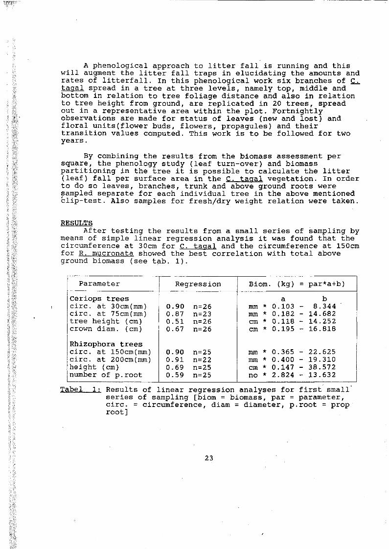
A phenological approach to litter fall is running and this will augment the litter fall traps in elucidating the amounts and rates of litterfall. In this phenological work six branches of C . tagal spread in a tree at three levels, namely top, middle and bottom in relation to tree foliage distance and also in relation to tree height from ground, are replicated in 20 trees, spread out in a representative area within the plot. Fortnightly observations are made for status of leaves (new and lost) and floral units(flower buds, flowers, propagules) and their transition values computed. This work is to be followed for two years.
By combining the results from the biomass assessment per square, the phenology study (leaf turn-over) and biomass partitioning in the tree it is possible to calculate the litter (leaf) fall per surface area in the C . tagal vegetation. In order to do so leaves, branches, trunk and above ground roots were sampled separate for each individual tree in the above mentioned clip-test. Also samples for fresh/dry weight relation were taken.
RESULTSAfter testing the results from a small series of sampling by
means of simple linear regression analysis it was found that the circumference at 30cm for C. tagal and the circumference at 150cm for R. mucronata showed the best correlation with total above ground biomass (see tab. 1).
Parameter Regression Biom (kg) = par*a+b)Ceriops trees circ. at 30cm(mm) 0.90 n=26 mm * a b
0.103 - 8.344circ. at 75cm(mm) 0.87 n=23 mm * 0.182 - 14.682tree height (cm) 0.51 n=26 cm * 0.118 - 14.252crown diam. (cm) 0.67 n=26 cm * 0.195 - 16.818Rhizophora treescirc. at 150cm(mm) 0.90 n=25 mm * 0.365 - 22.625circ. at 200cm(mm) 0.91 n=22 mm * 0.400 - 19.310height (cm) 0.69 n=25 cm * 0.147 - 38.572number of p.root 0.59 n=25 no * 2.824 - 13.632
Tabel 1: Results of linear regression analyses for first small' series of sampling [biom = biomass, par = parameter, circ. = circumference, diam = diameter, p.root = prop root]

For C. tagal the sampling series was enlarged up to 116 trees ranging from 15 nun to 511 mm in circumference. Enlarging of the sampling series for R. mucronata has still to be done. For the final analysis, as is common in literature, an LN LN relation was worked out for tree circumference versus tree biomass (see tab. 2 and fig. 1). For seedlings of C. tagal a relation was worked out between shoot length and total fresh weight (see tab. 2) in order to estimate the amount of biomass present in the plots as seedling.
Ceriops tagal treesLN(biomass in gram) = 2.31 * LN(circ. at 30cm in mm) - 3.02 range of circumference: 15 - 511 mm n = 116; R2 = 0.98
Ceriops tagal seedlingsLN(biomass in gram) = 1.49 * LN(length in cm) - 2.55 range of length: 20 - 99 cm n = 69; R2 = 0.93
Rhizophora mucronata treesLN(biomass in gram) = 2.25 * LN(circ. at 150cm in mm) - 8.03 range of circumference: 42 - 230 mm n = 25; R2 = 0.93
Tabel 2: Overview of final regression equations on biomassestimations for Ceriops tagal and Rhizophora mucronata.
biomoss fresh weight kgtoo
10
.0.1
0.0110 100 1000
circum ference of trunk at 3 0 or 150cm
° Ceriops togol Q Rhizophora m ucronata
Figure 1: Biomass fresh weight versus trunk c i rcuinf erence at 30cm far C. taual and at 150cm far R. mucronata.
24
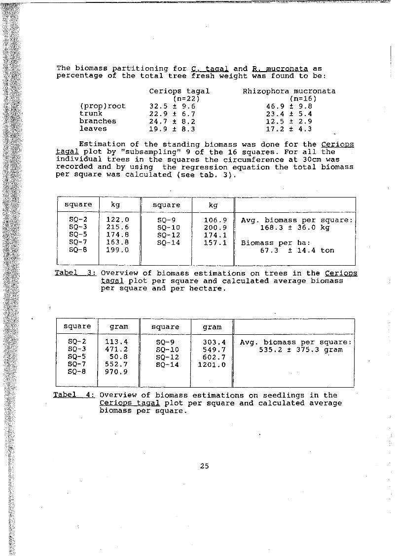
The biomass partitioning for C. tagal and R. mucronata as percentage of the total tree fresh weight was found to be:
(prop)root trunk branches leaves
Ceriops tagal (n=22)
32.5 ± 9.622.9 ± 6.7 24.7 ± 8.219.9 ± 8.3
Rhizophora mucronata (n=16)
46.9 ± 9.823.4 ± 5.412.5 ± 2.9 17.2 ± 4.3
Estimation of the standing biomass was done for the Ceriops tagal plot by "subsampling" 9 of the 16 squares. For all the individual trees in the squares the circumference at 30cm was recorded and by using the regression equation the total biomass per square was calculated (see tab. 3).
square kg square kgSQ-2SQ-3SQ-5SQ-7SQ-8
122.0215.6174.8163.8 199.0
SQ-9SQ-10SQ-12SQ-14
106 . 9 200.9 174.1 157 .1
Avg. biomass per square:168.3 ± 36.0 kg
Biomass per ha:67.3 + 1 4 . 4 ton
Tabel 3 : Overview of biomass estimations on trees in the Ceriops tagal plot per square and calculated average biomass per square and per hectare.
Í
square gram square gramSQ-2SQ-3SQ-5SQ-7SQ-8
113.4471.250.8
552.7970.9
SQ-9SQ-10SQ-12SQ-14
303 .4549.7602.7
1201.0
Avg. biomass per square: 535.2 ± 375.3 gram
Tabel 4: Overview of biomass estimations on seedlings in the Ceriops tagal plot per square and calculated average biomass per square.
25

LEAVES/BRANCH/WEEK0 .3
0.2
- 0.1
- 0.2
- 0 .3Dec 4 Dec 31 Jon 29 Feb 26 Mar 2 6 Apr 23 Moy 21 Jun 18
DATE
- © - n e w —S - LOST
Figure 2 ; Average number of lost and new formed leaves per branch for £e_rj.p p g_ t .a g a 1,.
The combination of biomass information and leaf phenological data are worked out to give litter fall rates and amounts in the C. tagal plot. The results and procedural information are as presented below.
From page 3 it is seen that 19.9% of the stand biomass is invested on leaves. So we can calculate the average biomass on leaves per square:
average biomass per square * 0.199 =average biomass on leaves per square
number of leaves/square =(biomass on leaves per square)/I.41a
From the phenology data it is possible to translate the number of fallen leaves per branch per week into fallen leaves per leaf present.
(lost leaves/branch/week) + avg. number of leaves/branch = lost leaves/leaf/week
26

As litterfall is normally presented in literature as dry weight per hectare per year some other factors should be added in the calculation:
litterfall [g dry]/square/week =(lost leaves/square/week) * 0.49b
[a: avg. fresh weight of individual leaf, b: avg. dry weight of individual leaf]
Biomass/square is between 132.2 and 204.3 kg (see table 3)1/br 1/br/w 1/1/w leaf biomass
per square (kg)DATE All lost lost min max
04-Dec 9.3 0.17 0.02 26.31 40.6517-Dec 10. 3 0.13 0.01 29.14 45.0231-Dec 10. 3 0.19 0.02 29.14 45 . 0215-Jan 10.3 0.16 0.02 29.14 45.0229-Jan 10.2 0.13 0.01 28.86 44.5812-Feb 10.0 0.15 0.02 28.30 43.7126-Feb 9.7 0.23 0 . 02 27.45 42.4012-Mar 9 . 2 0.11 0.01 26.03 40.2126-Mar 9.1 0.14 0.02 25.75 39.78
leaves lost leaves per litterfallper square square/week gram dry weig(number) (number) square/week
DATE min max min max min max04-Dec 18663 28830 341 527 167 25817-Dec 20670 31930 261 403 .128 19731-Dec 20670 31930 381 589 187 28915-Jan 20670 31930 321 496 157 24329-Jan 20469 31620 261 403 128 19712-Feb 20068 31000 301 465 147 22826-Feb 19465 30070 462 713 226 34912-Mar 18462 28520 221 341 108 16726-Mar 18261 28210 281 434 138 213Calculated out of the above tabel the average litterfall is
between the 154 and 238 gram dry weight per square per week. Onan annual basis this will be:
minimum 154 * 52 * 10000/25 = 3.20 ton/ha/yearmaximum 238 * 52 * 10000/25 = 4.95 ton/ha/year
27

DISCUSSIONOur use of measurements incorporating the two regression
equations of circ. 30 (C. tagal) and circ. 150 (R. mucronata) is consistent with what appears in literature for the use of dbh (diameter at breast height) and height in predicting stand biomass. Circ. 30 for C. tagal proves better on two grounds: for one it gives a high accuracy of prediction (R2 = 0.98 in In:In), and two the scrubby nature of the plot does not favor the use of dbh. Circ. 150 similarly gives a high accuracy (R2 = 0.93) and encompasses the majority of observations. The prop root development in the R. mucronata exclude the availability of stems at lower levels. Despite the good fit in circ. 200, it presents practical handicaps for its use and will in addition exclude several trees.
The biomass distribution in C. tagal seedling is so diverse (biomass per square = 0.54 ± 0.38 kg per square) that no conclusive remarks can be advanced now. Instead a call for
f further research in the line of seedling dispersal, growth and survival strategies is made.
From our phenological analysis for the period December 1990 to March 1991 the calculated dry weight of litterfall is in the region of 3.20 to 4.95 ton per hectare per year. This amount is some 6% of the dry weight stand biomass (52.9 to 81.7 ton/ha).Our estimate of 3.2 to 4.95 ton/ha/yr corresponds to what has been referred to as basin mangroves in related work by Twilley R.R et al.(1986) in the mangal wetlands of S.W. Florida. Indeed C. tagal has all the characteristics discussed for basin type mangroves. Basin mangroves have lower water turn-over, occupy inland sites that are less frequently inundated by tides and it is hypothesized that these sites have organic matter and nutrient cycles characteristic of more closed mangrove ecosystems. At a later stage it would be interesting to see if the values for R . mucronata also corresponds to the fringe and overwash type.
The links between primary productivity and storage and/or export forms another theme of this project which will give a good insight to the budget of the production. The stored component is to sustain the living system while the export component supports the off-shore productivity through nutrient enrichment (remineralization), detritus food chain, and DOM. Backed with this it is also possible to tell the health of a stand, whether progressing or dying.
28

4 6 '/ ó
4.1.2. Relative importance of mangrove litter as nutrient source: preliminary results.By: A.F.Woitchik(x), J .Kazungu(2), R.G.Rao(x) and
F. Dehairs Í1)(1) Lab. Analytical Chemistry, Vrije Universiteit Brussel,
Belgium(2) K.M.F.R.I., Mombasa, Kenya
INTRODUCTIONWithin the context of this EEC project we are studying the
relative importance of mangrove litter as energy source to secondary and tertiary producers. This subject is not well assessed presently, especially in East Africa. Our objectives are to investigate on the nutritive value of mangrove litter and its decomposition as potential source of nutrients in the ^ecosystem. The project focusses on the mangrove of Gazi Creek, Ÿsituated 50 km south of Mombasa.
Our first step to study the input of nutrients by litter decomposition was to analyze the C and N composition of leaves of the same physiological age of the main species of the mangrove leaves in situ and in the laboratory and its nitrogen enrichment by biological nitrogen fixation.
RESULTSC and N composition of mangrove leaves
In November 1990, fresh leaves of Ceriops tagal, Rhizophora mucronata, Bruguiera gymnorhiza, Avicennia marina and Xylocarpus
granatum were collected from Gazi Creek. To obtain leaves of the i same physiological age, we always took the second new leave on a
branch, and this for different trees of the saïne species. Leaves were dried at 80°C and brought back to Belgium for analysis of C and N with a Carlo Erba NA 1500 Nitrogen Analyzer.
The results are presented in the Table below:C/N atomic ratio
Species mean ± ff* NRhizophora 80 + 10 20Bruguiera 71 + 10 18Ceriops 69 + 5 20Xylocarpus 40 + 8 20Avicennia 28 + 6 20
N = number of leavesThe ratios of the main mangrove species of Gazi, Rhizophora,
Bruguiera and Ceriops, are higher than C/N ratios for surface29
4
I
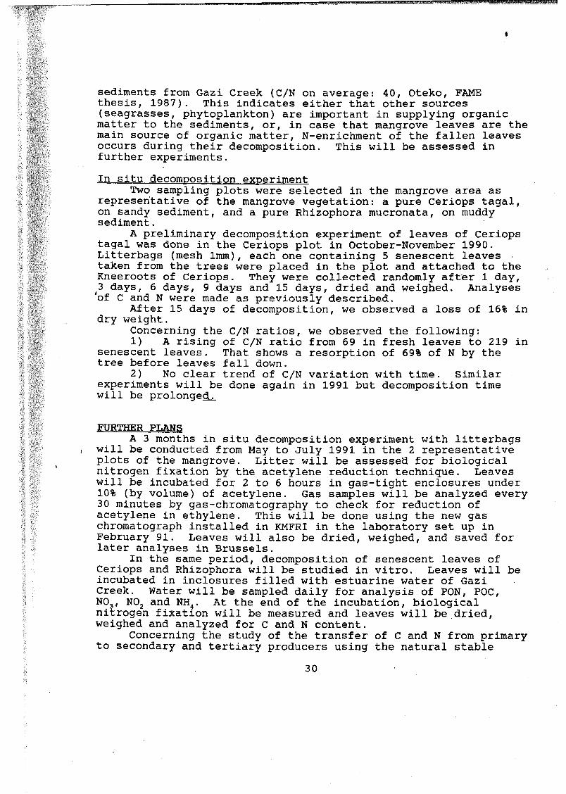
sediments from Gazi Creek (C/N on average: 40, Oteko, FAME thesis, 1987). This indicates either that other sources (seagrasses, phytoplankton) are important in supplying organic matter to the sediments, or, in case that mangrove leaves are the main source of organic matter, N-enrichment of the fallen leaves occurs during their decomposition. This will be assessed in further experiments.In situ decomposition experiment
Two sampling plots were selected in the mangrove area as representative of the mangrove vegetation: a pure Ceriops tagal, on sandy sediment, and a pure Rhizophora mucronata, on muddy sediment.
A preliminary decomposition experiment of leaves of Ceriops tagal was done in the Ceriops plot in October-November 1990. Litterbags (mesh 1mm), each one containing 5 senescent leaves taken from the trees were placed in the plot and attached to the Kneeroots of Ceriops. They were collected randomly after 1 day,3 days, 6 days, 9 days and 15 days, dried and weighed. Analyses 'of C and N were made as previously described.
After 15 days of decomposition, we observed a loss of 16% in dry weight.
Concerning the C/N ratios, we observed the following:1) A rising of C/N ratio from 69 in fresh leaves to 219 in
senescent leaves. That shows a resorption of 69% of N by the tree before leaves fall down.
2) No clear trend of C/N variation with time. Similar experiments will be done again in 1991 but decomposition time will be prolonged.
FURTHER PLANSA 3 months in situ decomposition experiment with litterbags
will be conducted from May to July 1991 in the 2 representative plots of the mangrove. Litter will be assessed for biological nitrogen fixation by the acetylene reduction technique. Leaves will be incubated for 2 to 6 hours in gas-tight enclosures under 10% (by volume) of acetylene. Gas samples will be analyzed every 30 minutes by gas-chromatography to check for reduction of acetylene in ethylene. This will be done using the new gas chromatograph installed in KMFRI in the laboratory set up in February 91. Leaves will also be dried, weighed, and saved for later analyses in Brussels.
In the same period, decomposition of senescent leaves of Ceriops and Rhizophora will be studied in vitro. Leaves will be incubated in inclosures filled with estuarine water of Gazi Creek. Water will be sampled daily for analysis of PON, POC,N03, N0Z and NH4. At the end of the incubation, biological nitrogen fixation will be measured and leaves will be dried, weighed and analyzed for C and N content.
Concerning the study of the transfer of C and N from primary to secondary and tertiary producers using the natural stable
30

isotope ratios, we are presently installing at the V.U.B. the new trapping box, linking the C and N analyzer to the mass spectrometer (Delta E, Finnigan Mat). J. Kazungu, senior scientist at K.M.F.R.I. will spend 3 months in our laboratory to learn the technique of mass spectometric analyses and to perform the first measurements of stable isotope ratios in different levels of the food chain in the mangrove ecosystem.
31

/ 4 6 7 b4.1.3. Nutrient dynamics in a tropical Mangrove Ecosystem
(Gazi Creek)By: J.M.Kazungu
INTRODUCTIONIn order to understand the productivity of any marine or
freshwater ecosystem, a study of nutrients availability and dynamics is of paramount importance.
Gazi Creek which is situated about 50 km South of Mombasa Island is essentially a mangrove swamp ecosystem. Mangrove species of the type: Avicennia marina, Rhizophora Mucronata,Xylocarpus granatum, Ceriops tagal and Bruguieria gymnorrhiza make up about 90% of the vegetation in the region. During low tides most parts of the creek are completely exposed and receive water only during high tides.
To the north, the creek is fed by River Kidogoweni which has been established as a seasonal river. River Mkurumuji which is located to the south of the creek empties its load to the open waters next the creeks entrance. However, theory has it that some of this load is ultimately washed into Gazi creek during high tide. If this were true, then the nutrients dynamics of Gazi Creek would actually be controlled by three sources, namely; River Kidogoweni, River Mkurumuji and the endogenic contribution mainly from bacterial decomposition of mangrove litter and seagrasses.
The present study which is still in its preliminary stages will focus on understanding and accessing the mangrove nutrient contribution to the ecosystem.
MATERIAL AND METHODSTo start with it was very important to know the distribution
of carbon and nitrogen contents in various fresh mangrove leaf species. For this, mangrove leaf species of Ceriops tagal, Xylocarpus granatum, Rhizophora mucronata, Avicennia Marina and Bruguieria gymnorrhiza were sampled and analyzed for carbon and nitrogen content. Samples were collected taking into consideration different physiological ages of the leaves.
As from January 1991. Sampling has been going on to establish nutrient levels within the water column of Gazi creek. Four stations G1-G4 (fig. 1) were established longitudinally across the creek.
32

RESULTS AND DISCUSSIONS:For the mangrove leaf samples, it was established
preliminary that there is no significant differences in carbon contents of leaves of specific species regardless of physiological age differences. However, older leaves were found to have less nitrogen contents (ref. earlier report).
Figure 2 gives a general picture of the nutrients profile in Gazi creek during the dry period. Generally, there seems to be an increase in nutrients from station 1 to station 4. If we assume that all this water is from the open sea which only fills in during high tide, then the nutrient levels are supposed to be uniform. The relatively high levels noticed in the inner part could only mean that there is an additional source of nutrients in the inner part of the creek. The higher nutrient levels could be attributed to River Kidogoweni being the only river in the northern part. This will have to be confirmed during the rainy season which have just started. The low nutrient levels between St.2 and G3 could be due to relatively higher consumption of nutrients by phytoplankton.
Figure 3 gives change of nutrients levels with time at St.G3. Sampling was started at low tide (February) and samples taken every two hours till high tide. Low tide was at 10.00am while high tide was at 3pm. At low tide when there was no influence of open sea water in the creek, relatively high nitrate, nitrite and ammonia values and low values of silicate and phosphates were observed. At high tide, the reverse was noticed. This implies that during high tide, water rich in phosphates and silicates and poor in nitrogen compounds is supplied into the creek.
FURTHER RESEARCH:Sampling will be done across the mouth of the creek
(transect between Chale Island and River Mkurumu'ji entrance) to establish how much organic matter and nutrients get into the creek during low tide. Longitudinal transects will also be made deeper into the inner parts of Rivers Mkurumnji and Kidogoweni and also across their openings into the Gazi creek to establish their seasonal input into the creek. Mangrove nutrient contribution will be assessed by following the decomposition rates of different mangrove leaf species and also changes in natural Isotopic (15N/14N) changes.
33

VG2
¡
I
'"■•«•Hud lend of a rv t/lj 3? Hinyrov« «S lol t r i Idai ftol vil h tttg r ijs (<30% )
1 * Mainland t Sublldal ItsgrtM l’ O* W0V.1 ÔJ1Î Wtrlidal fiai
Figure I Sampling Stations (GI -G4) in Gazi Creek.
34

sto
\
l/kON-N»®M$ó
BÖ 0-
10 - o
1/Ê0N-N ÖÖ
o*— o
1/ !S gu?Ös
<>5
ôR 20
-0 óóT*“» o
I/d jH-btt
0-60
0-50 5ö g
ód»c-JCi
tbT—Ó
ol/?HN-N»e-ß«Ö
pi gCMd>o«M» o
|/3Buj ^ S Öin oç>
••/.s £ R R o o
35
Figure 2.
General
picture
of the
nutrient
profiles
in Gaz
i Cre
ek during
dry period
(February
1991)*

oo«jri
.O Vi
oo
OO
Om o
1/-0N-N § O5 oo o o«M
oo o o
oo
o
36
Fig.
3 Changes
of nutrient levels against
time
at station
3. Low
tid
e was
at
10.00
A.K
while
high
tide
was at
3.00
EE.
(February
1991)
,

4 C 7 'f
4.1.4. Species composition and primary production of Phytoplankton at Gazi Creek B y : P . Wawiye
INTRODUCTIONThree representative station have been established along the
creek at the mouth (Oceanic), fish landing point and the head (inner mangrove). At each of the three stations measurements are carried out for primary production using the Winkler method. Measurements for biomass are also carried out using chlorophyll estimations. In addition other physico-chemical parameters like salinity, temperature and transparency were taken simultaneously. Samples for species composition and diversity were also collected through point sampling. This report includes a note so far w.r.t. productivity and the abiotic parameters.The average productivity of the three stations have been computed #to represent the creek productivity.
RESULTSIn the present study both the highest and the lowest
productivity occurred during the SE monsoon period, the lowest productivity occurring just after the long rains during the month of April 1990 (28.01 mg c/m /hr), while the highest productivity occurred well into the SE monsoon during the month of June 1990. (27 2.24 mg c/m /hr). It must be noted however that there were no values for the month of May. The average productivity of the Creek during the study period was found to be 129.02 mg c/m /hr.
The SE monsoon period was found to have a slightly higher average productivity (136.23 mg c/m /hr) than the NE monsoon period (109.44 mg c/m /hr).
The average water temperature during the SE monsoon was only slightly lower (29.1 C) than that recorded dufing the NE monsoon period (30.7 C).
Measurement of salinity recorded only a minor change in average salinity during the SE (35% ) as compared to the NE (36%) monsoon period.
Rainfall was high in March 1990, October 1990 and December 1990. In November 1990 their was a fall in Rainfall and the month of February 1991 was very dry. This showed some inverse relationship to the productivity which was low during the March - April 1990 (40.35 mg C/m /hr) and Sept. - Oct. 1990 (95.34 mg C/m /hr) period. In November 1990 their was a slight peak in productivity (156.17 mg C/m /hr) which fell until January 1991 (57.14 mg C/m2 /hr) to rise again in February 1991 (127.06mg C/M2/hr)
37
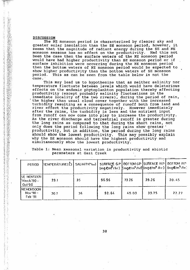
DISCUSSIONThe NE monsoon period is characterized by clearer sky and
greater solar insolation than the SE monsoon period, however, it seems that the magnitude of radiant energy during the SE and NE monsoon seasons has no effect on the productivity. Had this not been the case then the surface waters of the NE monsoon period would have had higher productivity than SE monsoon period or if surface inhibition were occurring during the NE monsoon period then the bottom waters of NE monsoon period would be expected to show higher productivity than the bottom waters of SE monsoon period. This as can be seen from the table below is not the case.
This may lead us to hypothesize that as neither salinity nor temperature fluctuate between levels which would have deleterious effects on the endemic phytoplankton population thereby affecting productivity (except probably salinity fluctuations in the immediate locality of the two rivers), during the period of rain, the higher than usual cloud cover together with the increased turbidity resulting as a consequence of runoff both from land and river effect the productivity negatively. However immediately after the rains, the turbidity is less and the nutrient input from runoff can now come into play to increase the productivity. As the river discharge and terrestrial runoff is greater during the long rains as compared to that during the short rains, not only does the period following the long rains show greater * productivity, but in addition, the period during the long rains should show the lowest productivity. This may possibly explain why the SE monsoon should have the highest productivity and simultaneously show the lowest productivity.Table 1: Mean xeasonal variation in productivity and abiotic
parameters at Gazi Creek
PERIOD TEMPERAT URE (C) S A IIN IÎY P /..} SURFACE G P(mg t /fT ? /h r )
BOTTOM GP(mgC/rrr’ /hrT
SURFACE N P (m g c /m 5 /hr )
BOTTOM N P (mgC/m*/hr;
SE MONSOON 'M.irch'90 - Oct’90
291 39 96.96H
73.26 39.26 20.45
NE MONSOON Nov ’90 - feb'91
307 36 92.6/. 49.03 39 75 22.77
38

PROD
UC
TIVI
TY(m
gC/m
2 /h
r)Figure 1.: Monthly variation in gross and net primary production
at Gazi
KEY
■o Gross productivity
■* Net productivity
300-
200-
. 100-
Mar Apr May Jun Jul Aug
1990 K 0 N.TH 5Period in which no sampling was done is shown using dotted line
Sep Oct Nov Dec Jan Feb Mar Apr1991
39

4.1.5. Zooplankton studies in a Mangrove Creek System. Gazi By: E.Okemwa, J.Mwaluma and M.Osore
OBJECTIVESTo examine the species composition of the Zooplankton community in the mangrove creek of GaziTo determine the geographical and temporal abundance and distribution of different Zooplankton groupsTo measure hydrographic parameters of pH, salinity, temperature, turbidity and dissolved oxygen and relate their effects on Zooplankton population
STRATEGYSampling stations are located at the creek mouth (stn 1), in the inner creek (stn 3) and intermediate (stn 2). Sampling is done twice a month; it starts from station 1 through stn 2 up to stn ÎÎ. A 335 um mesh size net is towed in near surface water for 5 minutes and the sample preserved in 5% formaldehyde. At the same time the hydrographic parameters are measured. Laboratory analysis of the sample involves sorting out the Zooplankton into taxa and counting under the Wild Heerbrugg M3C microscope.
RESULTSHydrological Features :Temperature - Maximum surface water temperature of 32.3°c was attained in March. The minimum 25.5°c occurred in August. Station 3 recorded the highest temperature and stn 1 the lowest. The annual temperature fluctuation was low, typical of tropical
. waters. Temperature was high between December and March (Fig.. D. -Dissolved oxygen - This varies within the range of 3.87 and 6.90 mg/L. stn 2 maintained somewhat a higher D.O. than stn 1. The lowest D.O. levels are recorded after the rains in June and January (Fig. 2).Salinity - It is fairly constant at about 35% except in the rainy season (April and December) when it decreased (Fig. 3).pH - Fluctuation was within the range of 7.50 and 8.63. Similar patterns existed between the pH of the 3 stations. Generally, the pH drops during the rainy season (Fig. 4).
40

Biological Features :Total Zooplankton - The Zooplankton is rich and abundant at Gazi and about 40 taxa have been recorded (see Table 1). Monthly average abundance varies between 25 and 425 organisms/m . The copepoda group is the most important constituent of the Zooplankton, it forms 31% to 98% of the total monthly Zooplankton population (Table 2(a) - (c)). Other abundant taxa include brachyuran zoea, chaetognatha, amphipoda and appendicularia.Each station displays peak Zooplankton abundance of varying magnitudes (Fig. 5). Stn 1 displays a major peak in June and another smaller one in December. Stn 2 has a major peak in March and a smaller one in May. Stn 3 has two major peaks in March and January and a series of smaller ones in May, July and October.Diversity of Zooplankton community - On the Margalef Index, the diversity ranged between 2.00 and 4.53 units. The highest diversity (4.53) was observed at stn 1 in August. On average, s'tn 3 had the lowest diversity of Zooplankton (Fig 6).
DISCUSSIONGazi Creek supports a diverse Zooplankton community which is largely dominated by copepods. Other dominant crustaceans include brachyuran zoea, chaetognatha, amphipoda and appendicularia. Abundance is higher during and just after the rains (March-April-May and November-December) and low during the dry season (August).Occasionally, there is an inverse relation between Zooplankton diversity and abundance, suggesting either a dominance by few species or an influx of many species. This phenomenon occurs in
r different stations independently. Since the hydrography between stations along Gazi Creek does not vary significantly, it is evident that water quality does not affect the distribution and composition of the Zooplankton community; at least not in the dry season when there is no surface run-off. The determining factor may be that the organisms actively choose their environment using their body shapes.At low tide, little water remains in small pools along the creek (much so in stn 3). Organisms that can resist (due to their body shapes or otherwise) the pull of the currents, will remain in these pools (or even in the sediments) till the next high tide. The organism will therefore tend to be localized in that station in large numbers or will consistently appear in each sample. The dominant taxa during such occasions; brachyuran zoea, Oithona spp. and Acartia spp. (stn 1) and Pseudodiaptomus spp., Oithona spp. and Acartia spp. (stn 3) could be possessing a common special ability. Investigations continue.
41

APPENDIXTABLE 1 Zooplankton taxa recorded at Gazi
TAXA STN 1 STN 2 STNAnnelida
Polychaete larvae XX X XXPolychaetes XX X XX
AmphipodaHyperia XXX XX Xunidentified XX X X
AppendiculariaOikopleura XX X Xunidentified X X X
BrachiopodaCladocera X X X
Chaetognatha Sagitta spp.X XX X Xunidentified X X X
Cirripediacirripedia nauplii XX X X
Cnidariasiphonophora XX XX XHydromedusae X X X
Cumaceacumacea XX XX XX
Copepodacalanoida XXX XXX XXXcopepodid XXX XXX XXXcyclopoida XXX XX XXHarpacticoida X X XXMonstrilloida X X X
Decapodapenaeidae X X Xsergestidae X X X
Decapod larvaeAnomuran Zoea X X XBrachyuran Zoea XXX XX XBrachyuran Megalopa XX X XCaridean larvae XX X X
Insecta X X XIsopoda
Paragnatha XX XX XXunidentified X X X
MolluscaBivalve larvae XX XX XXXGastropod larvae X X XXPteropoda X X XXHeteropoda X XX X
42

TAXA STN 1 STN 2 STN 3Mysidacea
Mysids X X XXNematoda X X XXOstracoda XX XX XXPisces
Fish eggs XXX XX XXFish larvae XX XX XX
Stomatopoda X X X
XXX = abundant XX = common X = rare
43

670
8-45
820
7-95
7-70
7-45 * STN io STN 2 • STN3
34
30
00 Pig X
'STN 2
STN1
I i----- 1----Mi»f Apr Ma^ -Jun c\ o
Au
Figure 1,2,3,4: Monthly variation of temperature, dissolved oxygen,salinity and pH at Gazi between March 1990 and February 199 1.

1 1 1 1 1.0 f v IY- r-4 m H 1-4 1-1 N F-- rt f v rH
1 D 1 - c I t !"••• -1 i n 1 0 0-4 C '1 l i i i n N i n m m r-4 1 1 ( N t v I N O ' LO IOi a i i r- » » » » r » » » » » » » » » » ». r ' ». »
i u . i 1 ! t i
t o ot v
N ' 4 o fH to C -I o 0 ' •O ' o • 0 O ' O ' O ' o o o O ’
i <i i i i t o o P 'l 1 0 IO to l > Í ’ • IO
r_ tto O ’ o . A t i *N
1 C 1I «TÎ I
'■%! 1 4 O ’ O c-t -t o 1—4 i o o * N I D r*4 • t o * o I N O ' o o * c o i . ' ;
1 ' “ i 1 1*4 ¡ N o O o o o r o CO • o 1-4 o r-4 o o o CN o o o o 1—4
1 1 1 1
r v 1-4
1 1 1 1 t v o 0 1 > o i p (ƒ ' ■rH 'D l > - , 0 3 q p 0 3 o 1—4 t-4 'w ' - , 0
I N1 U 1 r t o 0 3 -.-4 N C 1 r-J H 1—4 O'* o 1—4 o o * o o i H r—4 O ' o CN
• i a i i » » ». » » r ». ». » » ». » ». » » » » ». ». ». » ».—4 i a i e o O O ' O ' o * 0 œ i^ i o * o * o •0» o O ’ O '
0o
C ' o O 'i ii i
IDL_
P1 1 i i
m i i rt 0 IO 0 t o ! > to N | > i > f v m 1-4 0 ' N 1 0 i o «'A 0 ' A ( A
i +-' i IO t l ! •’» IO t-4 tN » 4 r - t a - r-4 o * r-4 - t m o > r i 1-4 1-4 ’•J ' o *c 1 U ! »• » ». ». ». » r . » » ». » ». » » » » » » ». ». ». »H 1 O 1
i t0 o
fvto - 0 r * j o o t o o o * O ' o O ' o 0 O ' o O '
mi i 1 1
» ••
c 1 1o 1 1 O O 1-1 1-4 1*4 r-4 - - Í T—4 r-4 o * 1—4 1—A u o 1—4 I—! —4 O ' o 1-4
-P ! D 1 CO o -1 ■0 o * LO 1.0 i n O ' O ' LO IO o t o o O ' C ' I O o O ' o IO•X i a i i ». • ». r- ». ». ». ». ». » » ». ». ». » ». ». » ». ». ». ». ».
C 1 i n ! ■r -1 '.,1 ( 4 1-4 O T* o * 1—4 -r-4 o - o * o i n o * T-! •0 ' A 1,C ' O ' o
a i i i to N r-4— 1 i io i in i i I—I O IO N 0-1 'O 1-4 I D 1-4 o » r o l i o O ' IO 1-4 I- “*» N O 0 * o : '0 1 O ' 1 I -- O • * t-4 a - K * t v »-4 IO O ’ o t t - I.B O ' 1—4 1-1 0 * r :> c * o C ' O 'u 1 - i 1 »• »• ». »• »• r- ». ». ». ». ». ». » ». » » ». ». ». »- ». ». ».
! ‘ X 1 f \ «'j i i-4 í n » - j O ' 1.0 -r-4 r o T—4 O ’ r-4 o * l “ *' 0 » !■*% o o r-4 O O ' O 'p i ic i irçi i *P 1 ! Ul o r ' t t o C« r_. i t - 0 0 O ' l ' - ' t-'l to o O ' A r ,-3 O ' O ' o * oL ! —4 1 1-4 O ' V)1 ( 0 fv.. IO i--! f-*r => D ' O ' D ' •43 o N . O ' O ’ O ' 0 ’ O ' O ' O '(3 ! ! » •r- » . ». ». »• ».
a 1 ! -H C ' r - - *•*; •.“ I* i r . i O ’ O ' O ' O ' t—A c » -r-4 O ’ o * O ’ o r-4 o ■A
E 1 ! t'-H ! !
i t
f -I I1 i n o IO Í.0 r • ; ! 0 r o 0 o hO O ' r o to o o O ' o o O ' o o
0 i r I i n o 0 4 IN V i t-A I.--4 1-4 0 3 O ' 1-4 1 0 t—4 t-4 o O ’ C ' o o * o * 0 ' O '! 5 1 »• ». »• » ». » ». ». ». » ». ».
c 1 ' - I 1 i N o — i O ' O O C-4 C ' O ' 1-4 0 * O ' o » o O ’ 0 « o * C ' 0 ' C » A t o *0•H
1 1 1 1
pr-4 1 1 » 4 "■'I ' 0 •—A r ’ t i - i o * N IO 1 r o 1—4 r-4 C ' 1-4 1-4 to C ’ O ' C 'm 1 > , 1 5 ó to l l ' l i n i* "A ó .•H o r o 1 0 IO r - l -D Ö 1—4 1-4 0 ' •J3 1-4 o O ' C -’0 1 a i I » *• *• r » *•■ ** •- JT ^ - T * ' I 'u I it '. I m o - t o to O ' O ' '0 ' o * O 1 O ' O ’ I N o o * o O ' O ' o O ' O 'gn
i Ii i
| v 1-1i.JU
i iI 1I I 0 c -I •o* -,-4 ,—1 K-'l
- 0 '0 ' O '- o * ■ 0 T—4 C;4 1— 1 o * O ' 0 3 r F 0 ' 0 * O ' NP 1 L ! ‘ 3 o * IO ■0 ■ 0 J-J\ 1 0 ' L-s O ' 1-4 IO c * O ’ '43 C ' O ' 133 O ' O ' O ' O 'C ¡ Ü 1 »• »■ ». »• » »- » »• ». ». » . V. ». W. »
PJ 1 - 1 1 i:o t * fv o o'* o ro o ■N to o t-4 O ’ O O ’ r-4 1-4 O * 0 ’ 0' r-4u i i inI !ai i io i 1 - 4 ro -t io in rv rt o o o io o -o to o o tv o o o o o oi t_ i to-io o to tv n io to o to to -< co o o o o o o o o rt
— 4 1 T. 1 o i i o o 1—4 .—i1-4O £. .'"■i »A Qc 1 1-p 1 1c 1 1 m a¡D 1 1 •r4 • r4 oSI 1 1 ai • r4 0 ai1 1 ní .c ai ai a¡ r-4 ( ■ 4 t ai1 1 a» -p m r—4 ai n a 05 Ô a¡•• 1 1 Í3 ni »a > a¡ Ji4-’ m 0 ai Xi »rn JO ai T3tf 1 1 a* l'-i c D ai r •o u ai a> a ITl 05 a? a •r4
*v 1 1 C3 m O' 0 U »15• r4 0 •rl aí ai CP 05 0 TI Z X. 0 tn •p1 tn 1 0 a* • ai 0 11 in i—4 •H a -o £. TJ ai ai •»4 • c 3 m maí 1 O 1 a in n a -p »a 2i r-4 r-1 C u 0 u ai ai • c 0 ai air-4 » J 1 aí 2» u •1-4 ai t r-4JZ O. .c ai □. .c a; e aí u c c cp aiD 1 0 1 G- n fTj f »a p r—4 m 3 a. 0. r-4 0 Ul e 0 c r_ a¡ a a rnj 1 Í. t 0 aí f Tl .n in 0 «-4 tí e Q 0 tti ■r4 3 +5 ai •r4 r 3 ait- I ra 1 1 fj jr ÜJ u u o 51 Z <x <L Ö. »—i Ll a CB ü_ rj i£ LO UJ co O
45

1I IO c T-l 0 0 C-4 fv r-. '0 •0 B -0 en O ro O -0 t-4 j
D 1 K C ■0 IO IO « C-4 r-4 0 0- Ü3 IO IO IO r-4 rji O' LO t-4 jai i
il I Ii
r- ct'-
l'i C-4 '-‘, C-4 ' Í t—4 t—4 o O o C' o t—4 1
11i fv 0 fr- 0- o- l> tr- o- 0- Q rx t-! ••*-. D- 1
c 1 ■—» C’ ri ■0 fr B O 43 fv K> •0 B o c o fr »U» o o o 03 1Oj 1 w r r r r w r r- 1
- I 1 tv o O K-“| o o* C-4 K' t i C-4 r i O* C' Q t—4 O o o fr 111
■-■0 tr—I
11 f r O fri f r fr ' t IO * ï B rv ■4 ■0 •fr o B O fr o o œ i
l.l 1 0 o ci fv rv fr n rv Cr- rt- r-- f-- • 0 C-4 »■“*1 ' t O' rv o o a- i• 0' 1
r-4 a i ! V O (r o .••■•, ■Ji C-4 o o t-4 o ■1 t—4 •0 t-4 I-*-, H o o o O o t—4 fI 0
C ii
in i C-4 o ro ■0 C-4 r> t—4 K* -r-4 CD C-4 C-4 IO N r4 N K |v C-4 £> iV r-j i1 n:i o 0 (B 03 o n- r4 O t—4 œ CD O Ul B m C-4 C-4 03 o O 10 !
c IJ 1 r » w r r r w V »N r w r. r rt r » w r r- r r- j■ri i
ifv O t-4 O t—4 t-4 ■H i- 4 C-4 O t-4 o t—4
i.n ic i0 i fv C* 0 !> >> r> a ül IO ÜO o l> Cr- o o tï- o o O i*“*» rx ip D 1 i> 6 o •0 -43 B •43 o* C' O* B -0 üO o* O O o ■43 O o r“*! ■0 Iùi m iÍZ • j:i i r i O io o o O* CJ r-4 C4 'C* o O* Ch 'w' Q o* o O o o O •'«.• iOi i '0 r-4
•■H in. iD i fv C' H o .41 I1.T 0' ' t •43 '0 C' -0 fv t> rv O O' o fv iV c* o* r*3 10 a ' i i J O 1-4 -43 i D -43 O O IO i”;. C-4 fv r-3 •fr O o* c* rv o o o O* IN ::¡ ! ■- r. r w. w IF. V r>. r- 9. rs rs tr. r *• r- }
i l I \o o r-4 C-4 O o ■»—4 o t—4 C-4 o C-4 —4 O o o o O Q. ’w* o Cr' 1•P i rv r-4r: ia» ip I i .» '•—* fv .■•••'i rv «> t-H fv -0 - t C' 13 ï> ro 03 c* o 03 O' £, O’ O' IL —« t O o 03 i-J -43 fr r-4 ir- •'i* r? rt •■•fr ro fr fr o o o O C' i-“;. J0 ' j 1 »• » w r- r. r- r- V. w- w. r- r- r. rs *• rs rs r. r- r- 1a '■'i 1 O fr IO r“-« rv o t—4 t-4 r -4 t-4 .;3 C-4 o Q o o* O o O o o ie 1
1-b r-4
•1-11 fv C' m O 0- O j o c , r-- O O ry- O o ,;■••, C- 1
o c: i r-4 LO fr IO 0- o fr o (ñ ' t IO ü"i o- ï> cr- C' o IO ÜO '■J? C' O I::¡ 1 r- *' r- r- r- tr- r. r- r- rs r- r. r- r- r f
c i O t-4 O1 c» o ro o o C-4 • » O 0 ’ O o c* o o O' O* o iCl
—1iI
I/O
■p I■ r~i ! fv O fr- r-4 fv o 03 r -1 O C-4 œ ixi Iv o o o O' to œ O O1 o im >. I r-4 fV p'5 ••43 io •■J? rv t—4 io o cr- t-4 t-4 Q3 o o •D C' r-3 •H i'V o O Io as i r- r r~ r- r. r- r. r- rs w- rs r. r- r. rs [□ r . i o i> f-4 t—4 o O1 'w O* r-4 O o O' O* o* o O C' O' o iE i IO t 30 iU i
i I/O o r-.i O r-4 fv O 4' O o r-3 O C’ et' •p» I> i4' !. I 0 o ••3 O 03 ro C' C-4 ÜO 03 o l'.Jf C-4 o C' 0' c-4 o O o o O* iC n i _••• -r ' *- J- - ** r- _•■• ■- *•• / * 1RI <r i 0 O 0- O o o o o* o* 'Z.' ;w' o* •-J’ O •-J' o o o •ij' o •!J' •O IUt ii 03
S iD. i f r !> i n d' •H 1X1 (X 04 t—4 03 p •fr t-l o o •!**’• £• o C 4 1
s. 1 a- K» fv K' ui o K» O •* t—1 C-4 o t—4 ■H ro o O' o o O o o O »>, ai i w- »• W r- r. r- r. r- w- W- r- r- r- V. rt r- «V •H r« r> rs r> r. 1-h m i IO O o o o o O O o O1 O* o* C' o O •3» o o O .V, O w* o iC i i>4-’ iC i aî 0)o i • r-4 r-4 o.
i ai S. •r4 0 aíi m c ai aí ai r—4 —1 r aii a? 4-’ ai r-4 05 T3 a a« 0 ai
•• i 0 05 aî > H3 n +J m 0 ai a» JZ aî •oX) i aí M C "D n5 r "O u ai a« a aí aî QJ a ■ r*4 • Ht-4 i u 0i a> n U ai -1-4 0 • H «a aí en aí 0 T3 z i : 0 tn -P
w i 0 ai . ai 0 u m r-l ■ f-4 a x j r xi ai ai +> •r4 • c d m m iai n i o, tn c 03 4> rtf Z3 r—4 •r» c u 0 u ai ai * c 0 a» ai r ir-i Zi i ai z> u r-4 ai r H JC O. r ai X a c ai E aî r u c c en ai rn 0 I O. t ) 0» f ai -p r-4 m Zi a a r~4 0 tn B 0 c L ai a D. t c t<15 - i. i o i ' 1 ai c in 0 ■m ai e a 0 m t*4 3 41 ai •M r •ri “1 ai p ri - ID I U £ ÍÜ u f j O H IL 2. <x <L LL »—4 IL u tn IL U Cù 03 tu 03 O 1
46

IOt:Plíl
wcD
c:ff;
(JDN
•Pc:«n5.o(jp•»-ocÜ
Í-1eoupcf!!b(0'ü—icpco
uCi
D0.1
I I
Cni
t iaid
Dai03
G«”1<C
>.fî:
Cl'1
mnIjO<*h
N o N K* ül m £, r-v r-7 O N ui o O K Ki 103 o 07 ^ r-J r-4 IO o I4“l/•7 t-4 io IO ro r-i o o O K.I r-, c« —i !» »• » » » r » r- » » ». » » » r r » 1r*4o - C' O •- ■' t—4 C' —4 o C' o ° o o ° o o r-4 I
c, IO -0 -0 N -rH K -0 t-4 rt 'i" et 0- o o t-4 I.-i o ■0 IO 0* C-4 O 03 C-4 t-4 i"i » 4 t—4 c* c î' o c* o CI Iw ». ». » r » » »• » » » » 1r“-i-t c> •47 C' *-3 O o c» c c, c* c« t—4 C c« 1
N T-1
IO o et O -0 K< -0 03 O C7 o Ul '43 O '41 O o c, 0 Ii"i o > :c. f> *t S- «i r-4 G' ■+ ro N K' ro o O1et Q' o o o r-v i» » »• r ». » r- 9, r- 9- » » ». » » ». » » » » r jIOf'v o -*-4 O O 43 ’H o o r-4 C-4 r-i t—4 C' o o o o o r-i i
»7' f 7 k •47 t-'l 47 Ki m r ;» 03 «t O '0 O f-o 1—( i1 1£* • “'i t'”*to C' i»! O t-- t—4 C' o t—4 o t-4 O o o o C' o o» » ». r r 9 r r r W- f- » ». » ». ». »• » » » » »• I03 Cy »'“*> o o •"¡iI'“-» o »■“*« O i"1! l‘*'lo o o o o j*>
lO o 0- et O «d: r-4 «t 0- “t o «t 0" Q o o o o o m i■0 c- -0 0" C”'a t—4l> -0 0- o •> ■J3 C' o o o o f"™'1t'-’«o *33 1» »• » f» 9 » r ». » » 9- » » ». jo Kl Q ;-•, T—1O K* «•"•i O Ki r”i O O • c* ••“■•io r—4 J
'• r-4
n c ri IO fi ■43 '43 Ul -43 C* 1'“'f t-4 et O Jr:» ° vr 1-4 io O 03 ° ?*'••C! ° 03 Ci il et O c» o ¡> ° o o O jK'n ° n c-i t-4 r*7 ° K t-4 C* ° •r-4 t-" r-4 o o ° ° «c
° i
et IO 1-7 03 T* 03 r-4 r-4 n 03 O 03 O fit ai r*-t 1j o rr - t 07 -0 0' h. —' »t *t t-4 ■ 14 i iT-4 |._t“4r-i C1r ■! c» Ir » »■ »• ». «F. ». r. ». ». ». » » r ». ». » » » » » » }
'i C ' O I-'7 ,— i o t-7 O1O* C* O c O r-i C' Ci C' O O1o c» c» c* i33
..o Ci Ci • -4 O 1.0 o C4 rj- r-4 r-4 Ul r-j o C- '■->o C1 -, 1> o IO 0 IO o r*"*»o O* 5 o ui '43 o IO O o o* o i». » ». w ». ». ». » » ». 9- i0 o O f-4 O C' C-4 o O Í-4 o r-4 00 c» O C' o o c* c i•t—4
0 07 K 07 <rt-ri 03 43 rn 0' o l> r :, O et o ro o 1
o 07 •0 1-7 et b 03 ef i 43 13 iJCl o -43 C' O O o* O et o '43 C’c* j» »• r • »• ■r- r. r- r- — r- ». ». ». r- V. -■ » 9- » ». » ». ». (a C' l-J "t r-4 o 'T o o ’O O T—4 O 1—1o o o 'wT O o r-4 o t*-, j7
/N O* C»11-7 03 M 03 't t—4 -0 ..—1C' C1c* io o N •c c« T—4 1t-4 t-4 C- O 43 C-4 iô K» '-t Kl O Ul o o c» o c* 1-4 C' o Ul i
». r- »• »• r- ». »• .. » » »■ ». r- ». ». » »• » » » ». »s 1"lO ¡■••j C* .—îO r-j o C-4 o r-7 ■H O O o o c T—1 C' o c* C' c ir-4
"io n r-i i-4 «-J-r-4 N 03 r -4 o et ro 0 —i Mt o i t-j. o - t—4 i—im t—4 t‘‘tC' o O o o o o o o■4o O O o o O -43 o o C' o o o o o o C’o o in t—4
ai ai■r4 -i a.ai t 0<li c ai a¡ aí r—1 »—4 r aiai -p n.i r-l ai TJ d. ai ô a»0 aí a¡ > ai 3 -p in 0 fli 3 ca r fl5 off? M c •o ai t TJ U ai en a aî ai ai a »4 •»4D ai ai a u ai * rW 0 rf m a: en ai o TJ z s: 0 m P0 aí . ai 0 u m t—* ■9* a -a JZ T! ai ai -p »4 • c 3 tn m iD. 1.0 c -o -P ai 3 r—•-i c u 0 u ai ai ■ r 0 Ti ai t 1a» U -i ai t r-4 r . O. r ai 0. r a e ai i- u x: .c O' ai i0. T1 ai î- ai P r-4 m “i a o. f—) 0 m E 0 c i- ai Ü. a e X. i0 ai L as -C l/l 0 •w aí E d 0 m H 3, -t-' ai •m 5_ »4 ai p* iJ j r uii u o O j: i . ~2L <x a. Cl f-» li U 03 X U tü w lu 03 o I
47

No
/D
iv
er
si
ty
(S
i
STN 1510
350
2-70
* STN Îo STN 2 • STN3
350
300
250
2001 5 0
,100
50
Jan Feb 1991
Nov DecMar Apr 1990 M o nth
Figure 5 Average monthly variation in zôoplankton population (nr/m3) and diversity of taxa at Gàzi between Mardh 1990 and February 1991.
48
4.1.6. Fundamental and Applied bacteriology in tropical marine waters.By: J.Wijnant,S.Mwangi and M.Owili
INTRODUCTIONThe study of the bacterial population,its activity and the pool of organic matter in the ecosystem is extremely important from a pollution and a public health view point»specially in regions with increasing tourist industries.Growing evidence show the quantitative importance of planktonic bacterial heterotrophic activity in the carbon cycle in marine ecosystems.Although it has often been assumed in the past that most of the produced organic matter flows through the zooplankton-fish tropic chain,it now becomes evident that planktonic bacterial activity constitutes,at least in some marine environments,a very important bypass.Therefore it is important in ecological research to have some knowledge of the basic relationships between organic matter and bacterial heterotrophic activity.Bacteriological research should emphasize two fields:l*the enumeration of marine pathogenic microbial populations 2*organic matter and activity of the microbial populations.
1.Infectious organismsAt this point we cannot discuss whether treatment plants,from an economic point of view,are effective in destroying infectious organisms,or whether other means of sterilization might be applied.Since it is desirable to keep the sea coasts hygienically clean as recreational beaches,the removal of communicable
i organisms from effluents in coastal areas is often more important than the reduction of the organic effluent load'.Particularly strict bacteriological requirements must be met in those areas where there are shellfish cultures in the vicinity of effluent drain pipes.Mussels and oysters filter bacteria out of seawater and often store them without the vitality of the bacteria suffering.Disease-causing organisms can only be found in bodies of water if prevalent in the human population.Escherichia Coli is under normal circumstances a non-pathogenic bacterium living in the intestine of man of warm-blooded animals»occurring in the faeces and therefore used as an index organism,along with some other faecal microorganisms.Faecal coliform germs are used to monitor sewage pollution and to asses health risks from drinking water,from food stuff,and from bathing.Escherichia Coli is always present in excrement and fecal effluents.Naturally,the presence of E .Coli in a body of water does not indicate anything beyond the fact that fecal effluents
49
are present in a diluted form.Civil health authorities in many countries of the world consider a ban on swimming if concentrations of Escherichia Coli higher than 100-1000 per 100ml are found in freshwater.Bacteria-eating unicellular organisms are in all likelihood hardly specialized in intestinal bacteria.However,they contribute among other influences to the elimination of Escherichia Coli because,under normal conditions,this intestinal bacterium cannot multiply in marine environment(Enzinger and Cooper 1976).When, however, seawater contains more than 100mg/l of organic substance, E.Coli grows and holds its own against marine bacteria.
TechniqueThe membrane filtration technique is now used as the best method for the enumeration of different pathogenic bacteria (method:see Wijnant et al.VLIR July 1990).
2.Biodegradable Organic SubstancesMan,like all animals,consumes organic foodstuff and leaves undigested organic remains behind in the faeces.In the preparation of his food organic substances are also left over as garbage,whether in the commercial processing of foodstuffs or as household waste.In natural environments,decomposers exists : organisms which specialize in the breaking-down of a dead organic substance.More precisely,they are organisms which satisfy their energy needs from dead organic substance.For the most part,they are bacteria and micro-fungi.Under ideal conditions,the cycle of carbon and oxygen is balanced in nature.When effluents from a city are introduced into a body of water,this means an additional supply of dead organic
i substances,and the question is whether or not it can be absorbed by nature.The number of bacteria in bodies of water can respond to the amount of available organic substance.However,bacteria consume oxygen in their respiration process.To serve as a rule of thumb,the Population-Equivalent Unit has been created;one unit represents the amount of oxygen that is consumed to break down during a 5 days experiment the readily degradable fraction of the faeces and garbage produced by 1 person per day.This figure is called Biochemical Oxygen Demand (BOD5).The term BOD describes either a quantity of organic wastes,or it refers to water quality(mg02/l).To identify the BOD of a water sample,first the oxygen concentration is analyzed,then the sample is maintained for 5 days at a temperature of 20 C in a closed bottle,and the oxygen concentration is again measured.From the difference between the two measurements one calculates the amount of free dissolved oxygen which has disappeared,the BOD.Within 5 days a reasonable fraction of the degradable organic matter in the sample is degraded by water bacteria.What is left
50

over are organic substances which are difficult to degrade;they could be analyzed by chemical methods(COD,Chemical Oxygen Demand).
3 .Ultrafiltration and carbohydratesWe can also study the relationship between organic matter and heterotrophic activity in aquatic ecosystems by determining their in situ concentrations and utilization rates of "directly usable low molecular weight molecules".Because in the most ecological methods it is assumed that heterotrophic activity is directly proportional to the "total organic load"determined as "biological oxygen demand(BOD)",chemical oxygen demand(COD) or total organic carbon,most of the organic load in sea water is known to exist as "dissolved organic matter"(such as sugars and amino acids). Dissolved organic matter can occur by phytoplankton and Zooplankton excretion and detritus hydrolysis by exoenzymes. However organic matter in seawater consists of macromolecules with molecular weight higher than 400 or 500 Daltons.The penetration of an organic molecule across a bacterial wall is an active process occurring with the intervention of specific enzymes called permeases.Only low molecular,weight organic molecules (monomers or small polymers)can therefore be taken up,the oxidation of the DOM happens through oxidants like oxygen and nitrates.Only through the production of exoenzymes,for example exoamylase,exoprotease,particles of H.M.W. molecules can be ultimately absorbed by bacteria.Phagocytosis of particles is not developed by bacteria.Therefore the pool of directly usable organic matter is the pool of L.M.W. molecules.So ultrafiltration of different samples on different membranes of
i different sizes will give us an idea about the concentration of carbohydrates in the different fractions of molecular weight
RESULTS AND DISCUSSION1.Results for the BOD 5 days and Dissolved oxygen The results are obtained by using the Winkler method.The method gives information about the total rate of oxygen consumption by the plankton community.So the results give us an idea of the nutrient mineralization in 5 days.The method is based on the calculation of the oxygen concentration(method:see Wijnant et al;VLIR JULY 1990)
51

1.1 BOD5 values TUDORThe values mostly ranged between 120-500 mgC/m3 in the four sampling points.However there were high peaks in Oct.90 and Feb 91 where the values were as follows: stl:60 mgc/m3 in Oct 90
788 600
st2:600 555
S t 3 : 60 st4:60
645
Feb 91 May 91 Oct 90 Feb 91 Feb 91 Sep 90 Feb 91
(See graph 1,2,3,4,5)
1.2. Dissolved oxvqen - TUDORAmong the four sampling points in Tudor creek there was no marked variation in dissolved oxygen as given per sampling date (see graph 6)In all the stations,the amount of dissolved oxygen was between 5,00 and 7,00 mg02/l except in very few occasions where the values were higher (10,24 mg02/l in station 1 ;8,32 mg02/l instation 2 ;8,96 mg02/l in station 3 ; 7,68 mg02/l in station 4"November" and 8,48 mg02/l "Feb 91)In general ,the average dissolved oxygen values were not very high but there were notable high peaks in November 90 and in December 90.There is also a small peak in February 91.(see graph 1,2,3,4,5)
Conclusion for Tudor: the concentration of biologically oxidizable organic matter present in Tudor creek is quite the i same in the four stations and if we compare the results with those taken in the North Sea (640 mgC/m3) a couple of years ago we can conclude that the amount of biologically oxidizable organic matter is low.From the data available,it is difficult to draw comprehensive conclusions on the relationship between dissolved oxygen and B0D5.Currently,the biomass of total heterotrophic bacteria is being determined in the sampling points in function of time.This will avail more information that will be useful in establishing a general trend in the creek.
52

1.3.BOD5 values GAZIThe values for B0D5 range between 120-500 mgC/m3 with some exceptions where the values are higher than 500 mgC/m3.In general station 1 (deep in the mangroves) reflected comparatively higher activity (see graph 7,11).Like in Tudor creek it is difficult to draw comprehensive conclusions on the relationship between dissolved oxygen and BOD5.As in Tudor creek the determination of the biomass of the heterotrophic bacteria is being carried out.
1.4. Dissolved oxygen - GAZIThe amount of dissolved oxygen ranged between 4,00-7,00 mg02/l in the four sampling points except for june where the values are slightly higher than 7,00 mg02/l and December where the values were higher than 8,00 mg02/l.In general,the average value of dissolved oxygen was about 6,00 mg02/l except for a small peek in October and a higher one in December (see graph 12)Stations 1 and 4 (both in the mangroves)registered comparatively higher values than the other stations 2 and 3.
2. CarbohydratesThe mean value for the concentration of carbohydrates in Tudor creek is 5000 mgC/m3 (5)The following are the mean values : station 1 6000 mgC/m3
station 2 4000 mgC/m3station 3 4500 mgC/m3station 4 4000 mgC/m3
The mean value for the concentration of carbohydrates in Gazi creek is 4500 mgC/m3 (4)The following are the mean values : station 1 6000 mgC/m3
station 2 6000 mgC/m3station 3 3000 mgC/m3station 4 3000 mgC/m3
These values are quite high when compared with the B0D5 values.This suggests that most of the dissolved carbohydrates are long chain molecules which are not easily acted on by bacteria. Further investigations will be carried out through ultrafiltration technique so as to determine the concentration of the easily degradable low molecular carbohydrates.
53

3. Pathogenic bacteriaThe mean values for the number of Escherichia Coli in Tudor creek are:station 1 21/100 ml (10)
station 2 10/100 ml (9)station 3 37/100 ml (10)station 4 12/100 ml (10)
The mean values for the number of Escherichia Coli in Gazi creek are:station 1 7/100 ml (4)
station 2 6/100 ml (4)station 3 7/100 ml (4)station 4 6/100 ml (4)
The world Health Organization (WHO,67)states that no water sample should contain more than 1000 total coliform group (TC)/100 ml and the EEC guideline (council of the EEC 75) says that no more than 500 TC or 1900 faecal streptococcal group per 100 ml
Conclusion:The number of E .Coli in Tudor is about 4 times higher than the number of E .Coli in Gazi creek.The existence of the few E .Coli observed in Gazi creek is due to relatively lower human activity as compared to Tudor which receives a lot of effluents from Mombasa town.In Tudor creek,a higher E .Coli count was observed in station 3 as compared to other stations.This could be due to possible discharge of sewage by the Coast General Hospital.
f
54

B0
0(m
grC
/m3
).0
2(m
g/m
3>
3
0C
(mg
rC/m
3).
02
(mg
/m3
),3
íom
as
s(-
1 OO
C)
(Tho
usan
d s)
(Th
ou
san
ds)
TUDOR STATION 1B O D 5,02 ,B lom os9 m a rin e b a d versu s Ilm a
0,9 -
0,0 -
0 ,7 -
0.6 -
0 .5 -
0 .4 -
0 ,3 -
0.2 -
J u l-9 1A pr—91J a n —91O ct—9 0Ju n—9 0
DAYS□ B 0 D 5 + oxygon O b io m ass m a rin e b a c t
TUDOR STATION 2B 0 D 5 .0 2 versu s tim e
0 .9 -
0,8 -
0 ,7 -
0,6 -
0 ,5 -
0 .4 -
0 ,3 -
0.2 -
0 ---Jun—SO O ct-S O Jan —91 Jul-91
0 BODS +■ Oxygen 0 Biomass m arine boct
55

BO
0<
mg
rC/n
fi3
).O
2<
mg
/m3
).2
[om
aa
s<
«1
00
0)
BO
0<
mg
rC/m
3).
O2
(mg
/m3
).B
tom
as
s(-
ia0
a)
(Th
ou
sa
nd
s)
TUDOR STATION 0B 0 D 5 ,0 2 ,S o m o s s m arin a b o e l versus DAYS
0 ,9 -
0,8 -
0 ,7 -
0,6 -
0 ,5 -
0 ,4 -
0 ,3 -
0,2 -
3 3 ,0 5 3 3 ,1 5 3 3 .2 5 3 3 ,3 5 3 3 ,4 5(T ho usands)
□ B 0 D 5 4- Oxygen O B iom ass m arin e b o c l
TUDOR STATION 4B 0 D 5 .0 2 ,B io m a s s m a rin a bo c l,v e rsu s lim e
9 0 0
8 0 0 -
7 0 0 -
6 0 0 -
6 0 0 -
4 0 0 -
3 0 0
200 -
Jun—9 0 Oct—9 0 -Ian—91 Apr—91 O ul-91
□ B 0 D 5 +■ O xygen 0 B iom ass m a rin e b o c l
56

BO
O(m
gC/m
.3)
02
(mg
/rr0
* 10
)
TUDOR STATION 1 ,2 ,3 ,40 2 Tudor s ta tio ns versus lim e
8 0 0
700 -
6 0 0 -
5 0 0 -
400 -<
3 0 0
200 -
to o -
Oct- 9 0 Jan—91 J u l-9 1
D s t l + »12 O s t3 A s l4
TUDOR STATION 1 ,2 ,3 ,4BOD Tudor stations versus tima
8 0 0
7 0 0 -
6 0 0 -
6 0 0 -
400 -
3 0 0 -
200 -
100 -
J u l-9 1Apr—91Oct—90J u n —9 0
a »11 + »12 * »13 A »14

80
03
(mg
C/m
3),
02
(nn
g0
2/m
3“1
0),B
tom
(»10
0C)
3(m
gC
/m3
).0
Z(m
g0
2/n
n3
”1 0
).E
tom
(“1 O
OO
)(T
hous
ands
) (T
ho
usa
nd
s)
GAZI STATION IB0D5,0 2 ,Biomass marine bact.versus Mme
0 ,9 -
o.e -
0,7 -
0,6 -
0 ,5 -
0 ,4 -
0 ,3 -
0,2 -
Ju l M S e p —9 0 O c t—9 0 Nov— 9 0 J a n —91 Feb—91 M ar—91 Mcy—91 Ju n —91
O B 0 D 5 + OXYGEN 9 b io m ass ( * 1 0 0 0 )
GAZI STATION 2B 0 D 5 ,0 2 ,B iom ass m a rin e b a c t.v e rsu s tim e
0 ,9 -
0,8 -
0 .7 -
0,6 -
0 .5 -
0.4 -
0,3 -
0,1 -
Ju l-90 Sep-90 Oct—90 Nov-90 Jon-91 Feb-91 M ar-91 . Mcy-91 Jun-91
□ B0D5 +■ OXYGEN 0 b io moss ( *1 0 0 0 )

BO
O3
(mg
C/m
3).
O2
(mg
C2
/m.3
»1
0)
B0
D2
(mg
C/m
3).
02
(mg
02
/m3
"1 O
).B
tom
(-IO
OO
)(T
hou
san
ds)
G A Z I S T A T I O N 3B0D5,02,Biomass morir» bocl,versus lime
0 ,9
0.80 .7
0.6
0 ,5
0 .4
0 ,3
0,2
J u l - 9 0 S e p - 9 0 D e l—9 0 N o v -9 0 J o n -9 1 F e b -9 1 M o r -9 1 M a y -9 1 J u n -9 1
□ B 0 D 5 + oxygen O b io m ass m a rin e b o c l
GAZI STATION 4B 0 D 5 ,0 2 ,ve rsu s lim e
9 0 0
8 0 0 -
7 0 0 -
6 0 0 -
5 0 0 -
40Û -
3 0 0
200 -
100 -
J u l - 9 0 S e p -9 0 O ct—9 0 N o v -9 0 J o n -9 1 F e b -9 1 M o r-9 1 M a y - 9 1 J u n -9 1
D B0D5 + 02

C2
(mg
O2
/m3
-10
) B
C0
5<
mg
C/m
49
(T
ho
us
an
ds
)
' 'GAZI STATION 1,2,3 ,4
B 0 D 5 Gozl s ta tio ns ve rs u s tim e9 0 0
8 0 0 -
7 0 0 -
6 0 0 -
4 0 0 -
3 0 0 -
200 -
100 -
J u l - 9 0 S e p - 9 0 O c t—9 0 N ov--9 0 J a n -9 1 F e b -9 1 M o r -9 1 M c y -9 1 J u n -9 1
□ stl + 9(2 O 9(3 A 9(4
GAZI STATION 1 ,2 ,3 ,40 2 G a il s ta tio n s ve rs u s lim e
0 ,9
0.8
0 .7
0,6
0,6
0 .4
Out—9 0 S e p —9 0 O ct- 9 0 N o v -9 0 J o n -9 1 F e b -9 1 M a r -9 1 M a y -9 1 J u n -9 1
D s t l + s t2 O s t3 A s t4
60

EXAM
PLE
OF
A ST
AND
ARD
FO
R C
AR
BO
HY
DR
ATE
S
Ï
o
oCO
Ulcoo
-4Jc0)1_aí
OCN
Ocn co N (û in ^ cl cm (NOO O O o o o o o o o o
UJU 0^9 uoipujpo
6 I
volume
ín glucoseftt)
R Squared
0,982093 7

4.1.7. The Fish community in a mangrove ecosystem4.1.7.1. Fish Community and Fisheries studies of Gazi Creeks
By E.O. Wakwabi, in collaboration with M.Ntiba,B.Okoth, G.Mwatha and E.Kimani.
SUMMARYThe fish community of Gazi creek is studied by beach seining method.A sieve net, about 50 m long, 1 cm mesh size and 2 m deep is used in the shallow shoreline water of the creek during low tide.Most samples are limited to low spring tides with isolated samples during neap tides. Low tides are preferred to high tides as they have enhanced catch rates, and offer larger operational ground a long the beaches.Much interest is cast on the fish species composition, size composition, and the nature of food and feeding habits of a selected species. The occupance of young fish whose adult population is hardly met within the creek is noted with interest. Especially for Caranx ignobilis whose adults are usually associated with open (oceanic) waters.
Note: This report covers only the months of May and June 1990.The rest of 1990 was not adequately sampled and the part of 1991 is reported in Mwatha, G. K. and Kimani, E.
INTRODUCTIONGazi creek experiences strong tidal fluxes especially during the
i spring tides. The abiotic and biotic environment in the creek is therefore subject to oceanic influence. During" low tide, most of the creek water is fluxed out of the creek. On high (flood) tide, oceanic waters flow into the creek in a more or less stream like manner. Norconsult (1975) used floating drogues to show that tidal currents contribute to the overall distribution of floatable into and out of the Mombasa creeks. This mechanism has been shown to play a vital role in the transportation of fish and crustacean eggs and Larvae between the offshore marine waters and the inshore creek waters, and hence important in serving nursery grounds (Garcia & Le Reste, 1981; Motoh, 1981; Staples, 1985; Subrahimanyam, 1965; and Wakwabi, 1988).Many species of mangrove fish move into mangrove areas at a particular stage in their life history (usually as larvae, post larvae, juveniles or spawners) and only associate with these areas during the stage. Others move in and out periodically (periodicity of tide etc) to feed. Such that, the success of many tropical fisheries depend on the health of the mangrove
62

swamps which mostly serve as nursery grounds and hiding (protection) grounds from predation e.g. Snappers, Jacks,Mullets, Sardines etc.To understand the ways in which human activities affect mangrove swamps, one must understand the influence man has on the environment. Man affects mangrove environment through e.g. fishery collections, mangrove harvesting, mangrove clearing for mariculture or agriculture purposes, indiscriminate discharge of untreated sewage, agro-chemicals etc.The studies on Gazi Creek will provide data and information on the utility of this creek by different fish species during any stage in their life history. Such information, together with the basic Oceanographic, Hydrographic, and Biological data may help in formulating management strategies relevant to the creeks ecosystem and useful for the establishment of overall management strategies for many more other ecosystems that share the same environmental, biological and fishery tenets.
RESULTSAs shown in the appended list, (Table 1) a total of 23 families of fish represented by 31 species was recorded. 18 of these species were represented by less than 10 specimens (got them represented by only 1 specimen). Goves oyena was the most prevalent, making up to over 46% of the total (748) number caught.Studies on the food and feeding habits are going on. Initial analysis show evidence that most of the fish caught during this sampling are juveniles whose adults are landed by the local fishermen fishing on the reef far out towards the open sea. The diets of those fishes varied a lot though it was clear that most of the species are feeding on the epibenthic fáuna, some on Zooplankton and only the siganids were found to feed solely on plant material mostly seaweeds (Table 2).
63

DISCUSSIONThe data displayed is very small and only represented in four samples dates. It's therefore not conclusive but may be seen as indicative of what the outcome of this study will provide.
TABLE 1FISHES OF GAZI CREEK
FAMILY1. APOGONIDAE
(Cardinal fish)2. BELONIDAE
(Carfish)3. BLENIDAE
(Belennies)4. CARANDIDAE
(Jacks)5. CLUPEIDAE6. FISTULARIIDAE7. GERREIDAE8. GOBIIDAE9. HEMERHAMPHIDAE10. LETHRINIDAE11. LUTJANIDAE12. MONACANTHIDAE13. MUGILIDAE14. MULLIDAE
, 15. PLATACIDAE16. PLATICEPHALIDAE17. SCARIDAE18. SIGANIDAE19. SCORPAENIDAE20. SHYREANIDAE21. SYNGNATHIDAE22. SYNODONTIDAE23. TERAPONIDAE
SPECIES Apogon sp.Archama lineolata Tylosurus leiurusPetroscirtes mitratus Omabranchus straitus Caranx ignobilisC. sexfassciatusHirklothychthis quadrimaculatus Fistularia petimba Gerres Oyena Gobius nebulosus Gobius spp. Heemirhampus far Lethrinus spp. Lutjanus fulviflamma L. johni Paramonacanthus barnardiPleromugil diadema Upeneus bensasi Upeneus sp.Platax pinnatus Platiaphalus grandidiers ?Siganus canaliculatusS . sutorScorpaena mossambica Shyraena jello Syngnathoides biaculeatus Saurida undosquamis Terapon jarbua T. theraps
NO. SIZE RANGE 112 2.5 - 7.421 3.1 - 8.44 36.5 - 45.56 3.6 — 5.71 6.1
22 6.2 - 9.77 6.8 - 10.72 5.7 — 2.62 15.5 - 17.2
348 1.7 - 10.56 4.4 - 7.5
64 2.5 - 6.55 5.7 - 35.5
45 1.7 - 5 . 72.4 - 8.4
34 ' 2.5 - 7.71 5.7!
1 14.31 7.91 8.91 4.61 6.41 5.8
26 3.1 - 6.61 2.3
23 3.7 — 7.315 6.8 - 29.57 7.1 — 11. 04 5.9 17.5
39 2.7 - 13.533 3.3 - 7.0
64

t VatM
I l i S l i !••
Ë K I K- • i<11>d)
H t )QiP s i l l a r : u
o c¡ ¡ ¡ l l l l l •H (0
1 i > r jV» T>
S K P -d) <t u
|®b |||C ' •H rHf Ë P l l i 1- f i m
I k .•*“4> vnUm
f ll§ |É fv n• 3
I V m r oo> o :i i
U i
I l l l l t l ^ >r i u»o o o■ri f i* > ¿1
•ü *Hr ; « jO HV t !
. r ; « nu o *A3r * • " !o H4 i P r jt o u i r-t
o«N
O.P.
U (Ul•üû) »-7O i< ui U01 0>r l r-0» Pi* r'M t/)|
(d»T»c n> MÄ
h %OA! HU. to
ynMSíoPiuic«
s*-«
O
fȔ1*1H
SfiM
S*J su
S!nM3MPig;(UIO
c «1a: M : j
. r•ü |J i ,o Al Alo
u< :»IO n C,' i o
m r : »■-i nr j VI « m At
oi P c i lfli « i AI ai
r-H U IO U I «JQ Û)»0 o
{H m *H C i
H
m3E]em Al
ri r 1c; <4 i<0 •HT* il4J •—(3 3•J «ii
VI•rl
«i: .rAl o»! cAS A3U •r
¿5

rrt A <Mi-i O «t OA r» A ri —« vo rs| 40R f B I 1 l i l i9 t ?*. r \ 3 ri fi m n h
Mh o r»(D -* m nB i i t 9 ri
m^inininor- t-. fj ri on n n *o »--< o ^ o\ m n m
r4 n r** • -f m «n rj■®r o o w*
i r- r- h «t Ci w Wh-'O.'fi 9t n r« ,o> eo f'* i m rj (j3p.rNHNN'*‘ w®iocoNy5Cor''ûn i n m•rf VC «) N ^ H ,\ß « N H H I
rnioco' m -f 09 rj ■• -r oI -H Os h* in
t- o t ch r gn ?"n o io nF" o fi o> fb- •+ *-• r*>
n n ori «i on n o ri m o
in to m er» »n 09tn M •“* |N •-♦ 1/1 'O Ul ’f m M r
M —■u AA As: U»0 A-1 V)3A O'T3 uA CA A Wy E c 73A 0A •—» ■H <0A — Ai >to t>4 —* -r.._ E c3 ü> 73IO w •—> 0 cA A E 0 A4_>Ai W tfl A>. s ü) <1)73 *■».C -C 7J 73 Oa o. O o tj 73o o d- r. a ci« ij m u h oÜ u D. *-» >*«J --• O W «)T. X u H O TO
i f vi »i -r ui 'O
A w> —fu — A (D — JC tf\
w w a — e o■~. Q) M ~* JC A LO H
W0 'O W O 73 9 O. C —< M O — a >* o o « j: u co
0)a*>ao<73GA
w- m
1)!2 a m 5 ® > M a ï S o -* u «M <0 » 5a~> -« o,—
« U M O O Di tl V 9 <h O « Ot M * M C >*jS «D 0U H ï w h o
« -S73 9 tfl C «3 ±J<0 mw G »— A 73a oe S o, a 9
0.82 9
c-w«tt A U A .Ou
9A»
n9O4i9A
t* WS O .C 73 a oO aíÖ g
o _ us »M « O ^ 9 73
ö ® s ç & 2 o V 9ï r; -S P .® g tj m m _ o51 ? 2 » & « e u r> ~ >•S S M p î « = .ho ®
— —. c— o>A 9 0« Ä 0Ai A (H A>•0 U JC O o O. A « 73 O aí » C
' » n ô 11 m >ü I a *9 " O ® S h u O A A a-as.ODomoawsusffl s: u 3 u *« * m
A A■*-> C— otfl N_ A A aí A M •«* > A C u a (71 A w O U W 0) W *i O M73 A 73
V) 0 •*- O 7373 W Œ O. 0 a> c—i .O Ai A A A OM A A O.— E SS M U O A A A
0)
73AC .r: cO 073A 4J «iA •_« Uw > 9 A cD. U tT» c: Ct»E A 0 A 0•-« “i ü n. 0F* 0) ■— AJC tfi 4i ti i»tfl 73 U) ww 0 •H73 0. •CJA U a 0 C E C*■» A 73 A A O ■*- 73 0a x: C D,— i 5* u cO Ü A 0 A A JZ A Á»7 Q r-n tj h m to to m
4 M fi l/l \o h1 ^ f< n 7 «/i «c r* r i »»i -r m \n
d)t)t:A1i
D 0)O UM •rltflXiW•r|M 1 RU fl)73 ttA 4-1 .rl4) F* roUA A-IA Ptfl RA•M tflOtnn•4JQA.riCn Hfi *—1r| -«H73 GA AA r».,h.73CA73OOTu
3
Ma:n
uMw
A94.)A»H9w U9 •r|a rHA An r:•H Atfl O
mfN
OHIO
SQMS5OMH
AOAMAXÍ
H
gQ
9 • C <3-i
Jf51
SOwm£Oitfl
AGm<i»u>.cotfl
í¿

4 6 8 'i
4.1.7.2. The fish community in Gazi CreekBy: N.Ntiba, Wakwabi, Okoth, Kimani, Mwatha
INTRODUCTIONThis study is a part of the EEC - VLIR - KMFRI mangrove
ecosystem project 1990 - 1993. The major aims of this study include
1) Study of the fish assemblage and the residence status ofeach species and for those fish that migrate from coralreefs, try to find when the migration occurs.
2) To study the feeding habits of these fish to elucidate food chain relationships within the mangrove ecosystem.
3) To study the importance of these creeks as a nursery habitatespecially for economically important fishes.
4) To study the physiological adaptations of these mangrovefauna.
MATERIALS AND METHODSBeach seining has been done at ebbing tide, flooding and low
tide to obtain samples for analysis. This has been done continuously from November 1990 to date.
The fish is collected in polythene bags and labeled indicating date and location of sampling along the creek. The sample is preserved for further analysis is the lab where it is weighed, sorted according to species. For large catches a
, representative sample is taken using the Dutch-Shuffle-method. Individual body weight, total length, standard length are recorded. The fish is then opened up for food analysis and gonad examination.
67

RESULTSDuring this study forty-six species of fish belonging to 28
families have been encountered (Table 1).Table 1. List of species and families of fish. Gazi Creek
November 1990 to April 1991.Family
1 Gerridae2 Sphyraenidae3 Tylosuridae4 Mullidae
5 Carangidae6 Clupeidae
'l Siganidae
8 Scaridae
9 Cephalocanthidae 10 Lethrinidae
11 Ostraciontidae12 Synodontidae
, 13 Anthrimidae14 Chaetodontidae15 Tetraodontidae16 Fistularidae17 Acanthuridae18 Monodactyndae19 Bothidae20 Gobidae21 Apogonidae22 Apogonidae23 Lutjanidae24 Pomacentridae sp.25 Anguillidae sp.26 Engraulidae sp.28 Sillaginidae28 Theraponidae
Species Gerres oyena G. punctatus Sphyraena jello Tylosulus acus Parupeneus barberinus Parupeneus macronema Caranx ignobilis Sadinella s p .Sadinella sidensis Herklotsichthys punctatus Siganus oramin Siganus sutor Siganus stellatus Leptoscarus vaigiensis Scarus iapanesis Scarus persicus Dactylopena orientalis Lethrinus harak Lethrinus nebulosa Lethrinus semicinctus Lactoria cornuta Paramonacanthus baranardi Saurida tumbil Saurida gracilis Preresus pinguis - Heniochus acuminatus Chelonodon laticeps Fistulania petimba Acanthurus lineolatus Ctenochaetus stigosus Monodactylus argenteus Bothus mancus Gibius keiensis Taenoides iacussoni Apogonichtys sulvensis Apogon hyalosoma Lutianus fluviflamma
Sillago sihama Therapon jarbua Therapon therops68
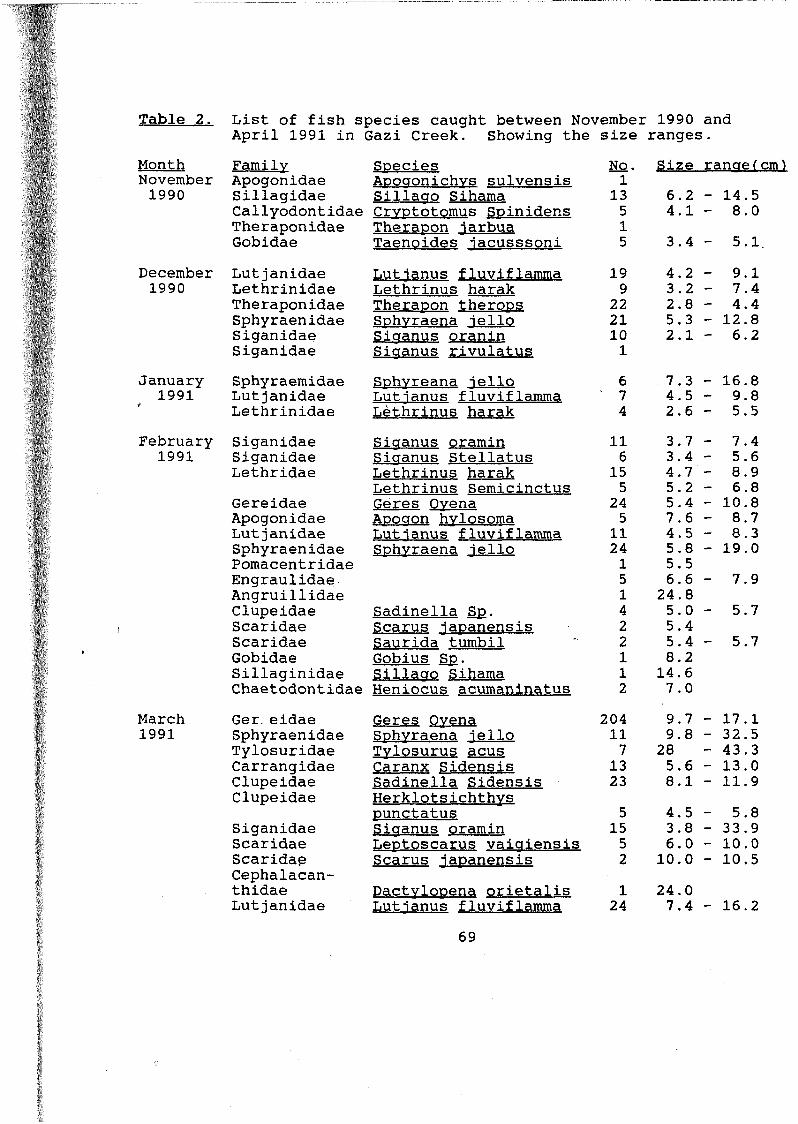
Table 2. List of fish species caught between November 1990 and April 1991 in Gazi Creek. Showing the size ranges.
Month Family Species No. Size ranae(November Apogonidae Aooaonichvs sulvensis 11990 Sillagidae Sillacro Sihama 13 6.2 - 14.5
Callyodontidae Cryptotomus Spinidens 5 4.1 - 8.0Theraponidae Therapon iarbua 1Gobidae Taenoides iacusssoni 5 3.4 — 5.1
December Lutjanidae Lutianus fluviflamma 19 4.2 - 9.11990 Lethrinidae Lethrinus harak 9 3.2 - 7.4
Theraponidae Therapon therops 22 2.8 - 4.4Sphyraenidae Sphyraena iello 21 5.3 - 12.8Siganidae Sicranus oranin 10 2.1 - 6.2Siganidae Siaanus rivulatus 1
January Sphyraemidae Sphvreana jello 6 - 7.3 - 16.81991 Lutjanidae Lutianus fluviflamma ’ 7 4.5 — 9.8
Lethrinidae Lethrinus harak 4 2.6 — 5.5February Siganidae Siaanus oramin 11 3.7 - 7.4
1991 Siganidae Siaanus Stellatus 6 3.4 - 5.6Lethridae Lethrinus harak 15 4.7 - 8.9
Lethrinus Semicinctus 5 5.2 - 6.8Gereidae Geres Oyena 24 5.4 - 10.8Apogonidae Apoaon hylosoma 5 7.6 - 8.7Lutjanidae Lutianus fluviflamma 11 4.5 — 8.3Sphyraenidae Sphyraena iello 24 5.8 - 19.0Pomacentridae 1 5.5Engraulidae 5 6.6 - 7.9Angruillidae 1 24.8Clupeidae Sadinella Sp. 4 5.0 _ 5.7Scaridae Scarus japanensis 2 5.4Scaridae Saurida tumbil 2 5.4 - 5.7Gobidae Gobius Sp. 1 8.2Sillaginidae Sillaao Sihama 1 14.6Chaetodontidae Heniocus acumaninatus 2 7.0
March Ger. eidae Geres Oyena 204 9.7 - 17.11991 Sphyraenidae Sphyraena iello 11 9.8 - 32.5
Tylosuridae Tylosurus acus 7 28 _ 43.3Carrangidae Caranx Sidensis 13 5.6 — 13.0Clupeidae Sadinella Sidensis 23 8.1 - 11.9Clupeidae Herklotsichthys
punctatus 5 4.5 — 5.8Siganidae Siaanus oramin 15 3.8 - 33.9Scaridae Leptoscarus vaiaiensis 5 6.0 - 10.0Scaridae Scarus japanensis 2 10.0 - 10.5Cephalacan-thidae Dactvlooena orietalis 1 24.0Lutjanidae Lutianus fluviflamma 24 7.4 - 16.2
69

Month
APRIL1991
Family Species N o . Size ranae(cm iLethrinidae Lethrinus harak 10 3.7 - 9.0Lethrinidae Lethrinus nebulosus 8 6.0 - 8.6Mullidae Parupeneus macronema 1 7.3Mullidae Parupeneus barberinus 3 17.4Ostraciotidae Lactoria cornuta 1 7.1 - 20.5Synodontidae Saurida tumbil 1 11.5Anthrinidae Preresus penauis 120 7.4 - 12.9Ostraciotidae Paramonacanthus
baranardi 1 3.6Chaetodontidae Chelonodon laticeps 1Fistularidae Fistularia petimba 1 37.1Siganidae Siaanus sutor 5 4.3 - 5.8Acanthuridae Acanthulus lineolatus 1 5.9Monodactylidae Monodaectylus araentus 5 7.4 - 12.4Siganidae Siaanus sutor 6 5.0 - 32.0Siganidae Siaanus stellatus 5 5.4 - 13.3Lethrinidae Lethrinus harak 36 5.7 - 11.8Lethrinidae Lethrinus semicinctus 18 5.7Tylosuridae Tylosurus acus 12 17.3 - 44.1Sphyraenidae Sphyraena iello 12 10.8 - 29.4Gerreidae Geres Oyena 359 ' 5.8 - 16.6Gerreidae Geres punctatus 2 14.6 - 16.8Acanthuridae Ctenochaetus striaosus 4 4.6 - 7.4Lutjanidae Lutianus fluviflamma 4 6.7 - 17.0Theraponidae Theraoon iarbua 8 4.8 - 9.4
Therapon therops 2 7.3Synodontidae Saurida aracilis 1 11.6Scaridae Liptoscanis vaiaienis 1 6.8Bothidae Bothus maneus 2 14.6Gobidae Gobius Keiensis 1 5.6
70
DISCUSSIONThe fish community in Gazi creek is diverse dominated by
members of a few families including the Gerridae, Theraponidae, Lutjanidae, Sphyraenidae, Siganidae, Lethrinidae, Scaridae and Mullidae. Occationally, migratory fish like the Anthrinidae and the Clupeidae School to breed or feed and dominated the catch. (Table 1).
Generally the fish size is small ranging between 5 to 10cm in length (Table 2). This is a clear indication that the creek fish community is dominated by juvenile fish since mature fish of the same species are hardly caught in the creek.
From the work done to date it can be observed that the number of teleost fish species is considerably less compared to other creeks in Kenya. Reay et al (1987) got a total of eighty three species while working in Tudor Creek. However work is still at the initial stages and no scientific conclusions can be made yet.
For our future work the sampling procedure has been altered. Thus from June 1990 sampling will be done in three definite stations (ie end of creek, mid-creek and creek month near the open sea) during spring low tide for three days every month.This alteration has been found necessary in order to a consistent and comparative set of data in order to achieve the objective set for this project.

4.1.8. SUBSTRATE INFLUENCE ON THE PHYSICAL AND CHEMICALPROPERTIES OF MANGROVE SOILS By: K.K.Kairu
INTRODUCTIONThe mangrove ecology is influenced by many aspects which
includes among others, the tidal cycle, seepage and altitude in relation to sea level. In non Mangrove areas, strong evidence of influence of soil salinity by soil type and water table have been documented. It is therefore of interest to investigate how the soil type influences salinity in mangrove areas, especially in regard to vegetation structure. To achieve this, areas with known different soil types were selected for the study.
The Gazi mangrove environment occupies a raised beach terrace ontop of which an alternating layer of sand and peat is observed. In Port Reitz, the creek cuts through Jurassic shales which have weathered to a thick clay horizon intercalated with peat in some areas adjacent to the channel.
METHODOLOGYIn each of the study areas fig.l, transects were selected
perpendicular to the main creek. Using a hollow plastic tube soil samples were collected, on the surface and a depth of 0.3- 0.5m at low tide.
In the laboratory, the water retention capacity was determined by drying to constant weight, samples of known weight. The clorinity was then determined by mixing equal weight of each sample with 20 ML of distilled water and centrifuging. This procedure was repeated twice. To determine how the levels of chlorinity in pore waters or films in the soil samples vary, it was assumed that the chlorinity recorded in the samples was .available in the liquid or solid phase in the wet sample.
SUBSTRATE CLASSIFICATIONThe collected soil samples were classified of the basis of
their texture and mineralogy into clays sandy clays sand or peat.OBSERVATIONS
Their is a strong relationship between, the substrate, water retention, clorinity and Mangrove structure (fig.2). Larger fluctuations are observed in the Gazi area. The clay and peat content appears to reduce clorinity extremes in both areas their is therefore an indication that their must be a significant relationship between the vegetation structure and the nature of substrate.The study is in progress and at the end of the rain season, it will be Interesting to investigate how precipitation affects the clorinity levels in the different areas.
72
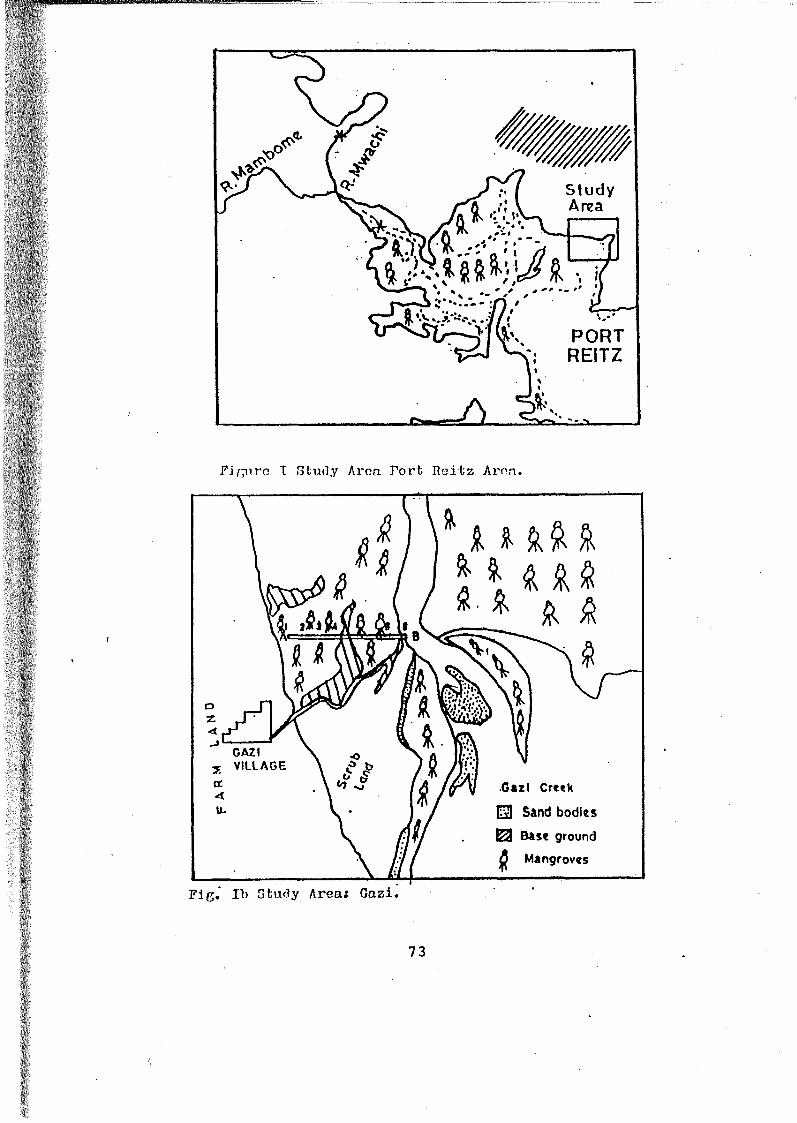
StudyArea
PORTREITZ
.— A
Fi/'Tiirc T Study Arca Tort Reitz Arca.
a. & &
ö \ * * *» s
»
-J G azi Creek
E l Sand bodies
EZ3 Base ground
jjj Mangroves
Fiß. Ib Study Area; Gazi.
73

PE
RC
EN
T W
ATER
C
ON
TEN
T P
ER
CE
NT
WAT
ER
CO
NT
EN
T
60Water c o n te n t Vs Ch lo r ide c o n te n t
GAZI
50 -
40 -
3 0
20 -
10
7 \
\ ' / 1\
/ / / ' zl
y//
6,7
4 NzsJ
4 ,2
\\
Ni
4,5
\
hN\\ |\
z\
2 8 ,9
\
K\ i\,KN ’ \
\ |\
h\\yV .
/ Z N
44,1
2 8 ,5
y— / *k N
/ \
51,1
\
/ n
2 2 ,9
Ii2 5 ,8
z7
/ ' X s
g
31 , I
2 5 ,7
z \7 7/ \
És tn 1 /s f b tm s tn 2 /s f b tm s tn 3 /s f b tm s tn 4 /s f b tm s tn 5 /s f b tm s tn 6 /s f b tm
STATIONS[7 /'i % WATER CONTENT \ \ l C l—/ K g S ubstra t«
<77
5 0
o Water c o n te n t Vs C h lo r ide c o n te n tPORT REITZ
40 -
35 -
3 0
25
20
15
10
I1 1,3
K /x//\xjv \\7//I\7
' /' 17► v
/ / /
4 :747
9,1
S
44,6
\ \ \ '
X, \7
V
V\
\ N
i
22,6
\ \7z
14
\ |
S.N
7 7
PC/
z
iz71
1,64
VN / /
16 ,9
\7 V
V '
V7
14,5
Z \ \ i
Z
s tn l / s f b tm
1/ /\ Ü «VATER CONTENT
s tn 2 /s f b tm s tn 3 /s f b tm
STATIONS
s tn 4 /s f
\ M C l—/ K g S ubstra te
b tm

4.2. RESEARCH IN THE FRAME OF THE VLIR PROJECT4.2.1. The distribution, growth and economic importance of the
Aqarophvte. Gracilaria (Gigartinales on the kenya coast. By: H.A. Oyieke
INTRODUCTIONAs stated in the last report this work is part of my Ph.D Thesis to be submitted to the University of Nairobi as soon as the work is completed. This study was divided into three major sections:
(i) The Ecology and Taxonomy of the genus(ii) Seasonality and growth studies
(iii) Agar Extraction and AnalysisV
RESULTS AND DISCUSSION i ■ The Ecology and TaxonomyThis section has more or less been completed though the voucher specimens of the species studied still need to be compared with those of other herbariums. Arrangements are underway to send them to Dr. Coppejans of the University of Ghent for confirmation of their identities. The ecology of the seven Gracilaria species, i.e. G. edulis, G. corticata, G. crassa. G. fergusoni.G. millardetii and G. verrucosa is now known. Different species were recorded growing in different habitats such as rocky pools, sandy pools, lagoons, muddy shores, rocky platforms, sandy channels and reef edges. The surveys revealed that there are no
, large expanses of Gracilaria beds at any one of the stations sampled that could be compared to those of the temperate regions. Most of the populations were found in discrete patches while some occurred as isolated thallus.Of the seven Gracilaria species reported only £. millardetii and (L_ edulis are strictly eulittoral whereas G . verrucosa is the only strictly sublittoral species. The rest of the species had some percentage of growth recorded in the eulittoral and partly in the sublittoral. Though greater percentage of crassa was observed in the eulittoral zone it would be in order to note that they were observed in pools under hidden crevices at reef edges thus indicating that they are exposed to direct insolation at any one time of the day. The temperatures in these pools were generally cooler than in the surrounding pools that were exposed at low tides. The fact that £. crassa pools were mostly situated at reef edges means that they were never exposed for long hours during low tides. Likewise GL_ corticata species that were observed in the eulittoral zone were found growing near the edge of the reef in pools that were never exposed for long hours
75

during low tides. In addition to this they were growing as epiphytes on lower parts of Thalassodendron ciliata thus being sheltered from direct insolation. The rest of the species were observed in the eulittoral zone where they were quite exposed to direct insolation during low tide. However, it was noted thatthe sublittoral population of Gj_ salicornia had more robustgrowth than the eulittoral population.ii. Seasonality and Growth StudiesThe results obtained in this study clearly show that the algal cover for both the £. corticata population at Gazi and at McKenzie was at maximum during the period covering September to March, while that for (L_ salicornia ranged from August to January. The maximum cover period for (¿. millardetii was July to January while that for (3¿_ crassa was July to December. The general trend in this study therefore, shows the period for maximum Gracilaria cover as that period covering the end of the South-East Monsoon season and the first half of the North-East Monsoon season.V
Figures 1-4 show the seasonality phenomenon observed in this study.iii. Agar extraction has been done on five different species namely £. corticata. G. crassa. G . fergusoni. G. salicornia and G . millardetii. These were the only species found in quantities large enough for extraction. In addition to that the harvesting for extraction was only possible during those months when they were in season.From the extractions done it is evident that SL. corticata had the highest agar yield followed by (L_ crassaf G. millardetii. (L_ fergusonii and GL. salicornia in that order. The results
, indicated a marked seasonality in the agar yield. At the moment arrangements are underway to carry out physical"and chemical analysis of the extracts before any report is given on the quality of the agar extracts.

PERC
ENTA
GE
ALGA
L CO
VER
FOR
G.
CO
RTI
CAT
A
LU
00- Ebo Wo oo o<0 ooCOoo»
(50tí3AOO TVO“IV
77
MON
THMC
KENZ
IE
POPU
LATIO
N +
GAZI
POPU
LATI
ON

PERC
ENTA
GE
ALGA
L CO
VER
FOR
G.
CR
ASSA
1
ooo> o o«0 oIO o'l- oCN o8 ott>
(S¿)tí3AOO TVOIV
78
SEP8
9 OC
T NO
V DE
C JA
N90
FEB
MAR
APR
MAY
JUN
JUL
AUG
SEP

PERC
ENTA
GE
ALGA
L CO
VER
FOR
G.S
ALIC
OR
NIA
oen
7 Ü4
O)oo
<D00O
C «)a 3 A o o iv o n vni ?
MO
NTH
MCKE
NZIE
PO
PULA
TION
+ GA
ZÎ PO
PULA
TION

ti
oútou .
D tU J>OO
<o<UJo<
2 !UJOQ tUla . r
o(Ooo oO) oIO o oIO oM o o
(5¿)HHAOO t v d i v
80
SEP8
9 OC
T NO
V DE
C JA
N90
FE3
MAR
APR
MAY
JUN
JUL
AUC
SEP

/ 4 6 8 4
4.2.2. Seaweeds of Kenva: a general survey of their economic potential alona the Coa .By : J . 6. Wakibia
INTRODUCTIONSeaweeds are of direct importance to man as dietary
supplement,food additives source of industrial feedstock and as a base of synthesis of a wide range of chemical products.Indirectly they are contributors to the natural food chain and habitats.
Kenya requires phytocolloids in the food industries,medicinal industries and agricultural practices.Kenya coast has a wealth of algae but meets its seaweed product demands through direct importation.These products era extracted from seaweeds,some of which are found on the kenyan coast.The lack of seaweed exploitation may be probably due to lack of information on the seaweeds of economic importance,their distribution and quantitative ecology.This study would try to give some cfuantitative and qualitative information on those seaweeds of high economic importance in kenya by studying their standing crop and front height.This information would be applicable for possible exploitation of the seaweeds by assessing and evaluating the present status of the stocks of economically important species of seaweeds.lt could also be used as a basis for formulation of resource management scheme to maintain and enhance the production of algae resources in kenya.
OBJECTIVESTo identify seaweeds of economic importance»measure their standing crop,percentage cover and front heights and documentation on their current uses in kenya.
METHOD.Thirteen(13) stations are used to represent the whole kenya coast.Abundance will be measured using the transect-quadrant method.A 50 by 50cm quadrant will be used for measuring the standing crops and percentage cover of the species of economic importance.The seaweeds harvested from each belt will be sorted,weighed to give wet weight and dried to in an oven for three days(3) at 105°C to give dry weight.
81

SUMMARYPreliminary surveys have to be conducted in Shimoni,Likoni,English Point,Kanamai,Vipingo, and Nyali. The positioning of permanent line transect is being carried out.Most of the common seaweeds in these stations have been collected, identified and herbaria prepared.The following observations have been made :Kanamai,Vipingo and Nyali are very rich in marine angiosperm vegetation notably Thalassia hemprichii.being dominant in the lagoons and Thalassodedron ciliatum near the reef edge.Others include Halodule wrightii and Halodule universi.Seaweeds especially the brown and red ones are partially distributed with Sargassum spp. and Turbinaria spp. within the coral region.and some Ulva spp. near the platform.
English point and Shimoni regions are rich in seaweed diversity and abundance.The most abundant species are Sargasssum spp..Ulva spp..Gracilaria Cystoseira Myrica,Laurencia pappilosa.Within the establishment of permanent line transect the quantitative survey will start using the permanent quadrant niethod.
82

/ 4 6 8 b
4.2.3. A comparative Study of growth and recruitment of selected coral species alona the Kenya Coast.By : J. Mutere
INTRODUCTIONThis project is being carried out at three study sites namely Malindi Marine Park, Vipingo and Kanamai. Malindi represents coral reefs that are protected whereas Vipingo and Kanamai represent unprotected reefs. Percent cover of living and dead coral studies at the study sites were carried out to determine the coral population structure. This is to form the baseline information from which recruitment and growth studies can be made.
METHODSStudies of the percentage living and dead coral done using the vline transect method. This was done during the low neap and spring tides and transect of 25m length were laid parallel to the beach. Data collected was represented by graphs (Appendices 1,2, and 3). Corals were collected for the institute reference collection, for from each study site. This was done by random swimming and collecting the corals by use of hammer and chisel, as each new species was encountered. Corals collected were bleached in a solution of fresh water and household bleach and then sun-dried and packed in labelled polythene bags for storage.
RESULTSThe Malindi study site has the highest percent cover of living coral followed by Vipingo then Kanamai. At Malindi percent living coral cover ranges from 8.6% to 58.86%^ at Vipingo, 6% to 24.2%% and at Kanamai, 2.86% to 16.4%. For pe'rcent dead standing coral cover, it ranges from 18.46% to 79.86%% at Malindi, 14% to 55.9% at Vipingo and 3% to 17.4% at Kanamai.The highest to lowest coral species diversity at each site was in the same order as for percent cover of living coral. Acropora sp appears to be the dominant genus at Malindi study site, Whereas Palauastrea sp is the dominant genus at Vipingo and Porites sp at Kanamai.Several coral genera are common to all the three sites namely Favia. Galaxea. Pocillopore. and Porites. However, the Malindi and Vipingo study areas appear to have more genera in common than with Kanamai, namely Acropora. Echinopora Favia. Fungia. Galaxea. Goniastre, Hydnophora. Leptoria. Pocillopora. Porites and Montipora.

DISCUSSIONThe variation seen at the three study sites in terms of species diversity and percent living and dead standing coral cover may be due to certain factors. One such factor is the differences in reef structures whereby at Malindi, the area under study is a patch reef but that of Vipingo and Kanamai sites are fringing reefs. The differences in wave energy and local currents are also other factors to be considered. The depths and differences in levels of exposure at low tide are also important in determining the community structure.The levels of human exploitation at the three sites varies in that Malindi is in protected marine waters and therefore not exploited for fishing and coral collection as the other two sites.All the aforementioned are factors that should be investigated more closely to give a better idea as to the factors governing coral community structure on the reef flats and lagoons of the Kenyan reefs.
ÇE.NU ?, U S.T
GENUS Hal Indi Vipingo Kanamaí
Acropora +AstreoporaCosclnareaCyphastreaEchinopora 4
Favia 4 4 4
FavitesFunqla 4
Galaxea 4 4 4
Goniastrea 4
Hydnophora 4
Leptoria 4
LeotoserlsLoboohvH laOxyporaPavona 4 4
PoclIlooora 4 4 4
Porites Es ammocora
; 4 4 4
Hontloorq 4
•Tubipora 4 4
ElatyqyraSeriatopora 4 4
GonioporaStylophoraH e rp o lith a 9 4
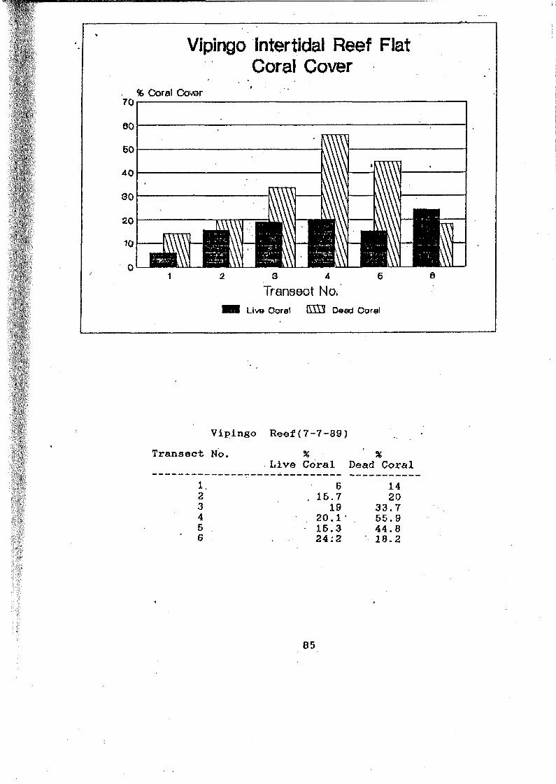
Vipingo Intertidal Reef Flat Coral Cover
% Coral Cover7 0 i----------------------------- --------------------------------------------------------------------------------------------------
00
1 2 3 4 6 0
Transect No.U v a Corel ( U \ l Dead Coral
Vipingo Reef(7-7-89)Transect No. % %
Live Coral Dead Coral1, 6 142 , 15.7 203 19 33.74 20.1' 55.95 15.3 44.86 24:2 18.2
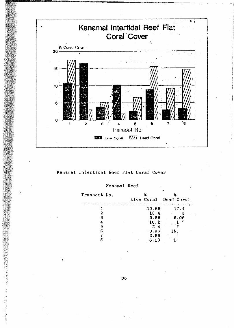
Kanamai Intertidal Reef Flat Coral Cover
20% Coral Cover
4 5
Transect No,U va Coral IM Y l Dead Coral
Kanamai Intertidal Reef Flat Coral Cover
Kanamai ReefTransect No. % %
Live Coral Dead Coral1 10.66 17.42 16.4 .33 3.86 6.064 10.2 1 "6 2.4 C6 8.86 16.7 2.86 . i8 3.13 I-
.86

JU
Malindi Coral Garden Coral Cover
% Coral Cover100|--------------------------------------------
Transeot No.Live Coral l i W i Dead Coral
M ndl ReefTransect No. % %
Live Coral Dead Coral1 38.33 18.462 8.6 64.23 14.53 24.66A 58.86. 39.46
48.73 35.8625.46 54.73
15 79.8624.66 67
87

/ 4 6 8 64.2.4. Assessment of pollution in the coastal and marine
environment around Mombasa4.2.4.1. Theoretical Assessment of the pollution sources and
loads of the Creeks around Mombasa By: J.Munga, K.Delbeke, S.Tsalwa, S.Mwaguni and J.Wijnant
INTRODUCTIONAs very little information is available on the state of
the Marine environment of Kenya a research programme "Assessment and control of pollution in the Kenyan Coastal and marine environment " was started. The programme is conducted as a collaboration between KMFRI, Kenya Government Chemist and KBP.It consists of different subprojects :-
1. Theoretical assessment of the pollution sources and loads.
2. Monitoring of pollution levels in the coastal and estuaries environments.
3. Assessment of the importance of pollution on the mangrove oyster, crassostrea cucullata.
For the theoretical assessment useful
RESULTS1.Domestic Sewage Disposal
The Mombasa municipality has separate sewerage systems for domestic sewage and storm drainage (fig. 2). The sewerage system for domestic sewage serves about 11% of the population of Mombasa. There are two treatment plants, for sewage disposal, (located in the island at Kizingo and the west mainland at Kipevu. The Kizingo plant is capable of carrying out primary treatment of sewage before discharge into the Tudor creek, and covers about 20% of the island. The Kipevu plant was designed for sewage treatment to the secondary stage, and discharges into the Kilindini creek. An estimated 72% of the population use pit latrines, and the rest (17%) use septic tanks and soakage pits for sewage and waste water disposal. Sludge from septic tanks is usually disposed off at the Kibarani dumpsite in the vicinity of the Makupa creek.
Data on the sewage strength at the outfalls from the treatment plants (GOK, 1974) and information on average sewage strength from septic tanks and pit latrines (Iwugo, 1990) was used to estimate the daily organic and inorganic pollution loads due to domestic sewage disposal, into the creeks around Mombasa (table 1).
88

TABLE 1: Waste from domestic sources
Disposal Pop. WV BOD,.b SS N P
System (103p) m3/cd103m3/d g / cdtn/d g/ cdtn/d g/cdtn/d g/dctn/d
Sewerage (a) Island 42 0 .0 7 a.. 11 4 4 .0 1 .8 5 280 11 .76 40 1 .6 8 10 0 .4 2
(b) West Mainland 13 0 .1 3 1 .7 0 4 7 .7 0 .6 2 90 1 .1 7 20 0 .2 6 10 0.10
PitLatrines 376 .32 20 7 .5 3 - - - -
Septic tanks/ soakagepits 89 .5 4 - - 30 2 .6 9 - - i
Pop = population WV = waste volume SS = suspended solids N = nitrogen compounds P = phosphorus compounds Units p = persons, tn = tonnes, cd = capita day (-) = no data available.
Although the sewage treatment works serve only about 11% of the' population, the effluent from the treatment plants has a considerable contribution to the pollution load. The level of treatment of the sewage thus needs to be seriously reviewed and appropriate improvements incorporated.2. Storm Water Runoff
There are 3 storm water drains discharging into the Tudor creek, and 3 other drains discharging into the Kilindini creek from the island and west mainland areas (fig. 3). The rest of the Mombasa area provides non-point sources of storm water into the creeks. For the purpose of estimating the contribution of storm water runoff to the pollution load, a runoff coefficient of 0.75 was assumed (table 2). The total surface area and mean rainfall were, 210 m2 and 1038 mm/year, respectively.
89

Tabic 21 Contribution of slora »ater runoff to pollution loadsRuno Í f
10Jm3/ km d
Vo 1 une
10V /d B/J m d
BODj
103kg/d
SS
g / kg /d m d
N
g/ kg/d m d
r
g/ Ad m d
2.13 4 4 7.3 140 62.62 430 201.3 5 2.24 3 1.34
The storm water runoff thus contributes significantly to the pollution load of the study area.3. Industrial Wastes
All Mombasa industries are considered as potential sources of pollution. The types of pollutants produced are organic degradable materials, suspended solids, nutrients, oils, heavy metals, detergent, etc.
Most industries also use septic tanks and soakage pits for disposal of domestic sewage and industrial sullage. Likewise, sludge from septic tanks is disposed off at the Kibarani dumpsite. Industrial liquid waste, that is most probable contaminated with toxic chemical is often allowed to discharge
' into the storm water drain and eventually into the creeks; for example, the Kenya oil Refinery. Some industrial establishments are however allowed to discharge waste into vertical drains that end on the water table. During flood tide, however, the drains sometimes overflow with unpleasant effects. Vertical drains are a potential source of toxic wastes which may seep unneutralized into the marine environment.
Pollution loads from some major industries have, so far, been considered. (table 3). The nature, quality and quantity of contribution to the pollution load varies according to the industrial processes carried out. The more extensive investigation of the pollution loads from all industries is being shore and data will be available soon.
laki« It {«atrlkitl*« «f Indaitrlil ictivltlti t« pallatlan 1»*il
Induatry Unit Inp/d Prod/d eooj kg/un 11 kg/d
d
SSkg/untt kg/d
d
Oilkg/unit kg/d
d
Phanal* - kg/unit kg/d
d
R ( tkg/unit kg/d
d
S RR kg/unit kg/d kg/unit k
d d
IRt tnlUI 71.0 - 6.1 072.0 S.S 001.3 - - - m •
U l * 3baar - 121.0 10.0 2,319.0 7.3 901.0 - - - -
StaalTuba* tn - 23.î 2.2 S I.2 2.32 S O.1 - - F 10.02 0.07 2nt0.007 1
FatO.19 ' Crtl.llS
tabra- uork» tn . < 1.0 0.0 0.1 01.1 00.0 • - - -
I0*‘ 103tn M l - I.SS 3.SS 0.67 3.07 0.16 0.02 0.1 o.ss - 1.0 S .00 Crit.09
Inp/d • Input/day. *r«d/< - praductlan/day, KX • haavy ««tali, I « - liv* uatght «f a n l n l i klllad,IRC • lanya Raat Canniailan «la«ghtar-houie, U l • lanya Iravarla* ltd. kaar nanafacturaa, IO* » lanya Oil latinaría*. • Data froa IO* to ba ravlauad.
90
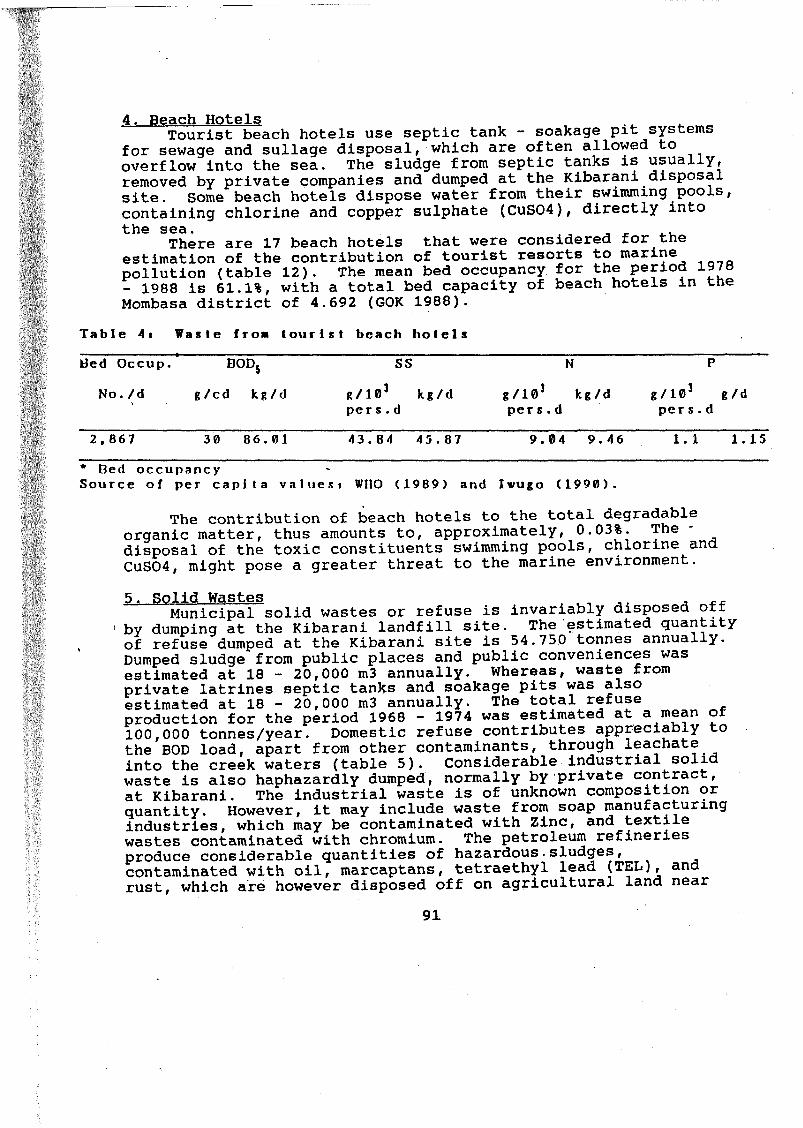
4. Beach Hotels .Tourist beach hotels use septic tank - soakage pit systems for sewage and sullage disposal, which are often allowed to overflow into the sea. The sludge from septic tanks is usually, removed by private companies and dumped at the Kibarani disposal site. Some beach hotels dispose water from their swimming pools, containing chlorine and copper sulphate (CuS04), directly into the sea.There are 17 beach hotels that were considered for the estimation of the contribution of tourist resorts to marine pollution (table 12). The mean bed occupancy for the period 197Ö - 1988 is 61.1%, with a total bed capacity of beach hotels in tne Mombasa district of 4.692 (GOK 1988).
Table 4. Waste froa tourist beach hotels
Bed Occup. BODj SS N P
No. /d g/cd kg/d g/103 kg/d pe r s . d
g/103 kg/d per s.d
g/103 per s.d
g/d
2 . 867 30 86.01 43.84 45.87 9.04 9.46 1.1 1.15
* Bed occupancySource of per capita valuesi WHO (1989) and Iwugo (1990).
The contribution of beach hotels to the total degradable organic matter, thus amounts to, approximately, 0.03%. The disposal of the toxic constituents swimming pools, chlorine and CuS04, might pose a greater threat to the marine environment.
5. Solid WastesMunicipal solid wastes or refuse is invariably disposed ori ' by dumping at the Kibarani landfill site. The estimated quantity of refuse dumped at the Kibarani site is 54.750 tonnes annually. Dumped sludge from public places and public conveniences was estimated at 18 - 20,000 m3 annually. Whereas, waste from private latrines septic tanks and soakage pits was also estimated at 18 - 20,000 m3 annually. The total refuse production for the period 1968 - 1974 was estimated at a mean of 100,000 tonnes/year. Domestic refuse contributes appreciably to the BOD load, apart from other contaminants, through leachate into the creek waters (table 5). Considerable industrial solid waste is also haphazardly dumped, normally by private contract, at Kibarani. The industrial waste is of unknown composition or quantity. However, it may include waste from soap manufacturing industries, which may be contaminated with Zinc, and textile wastes contaminated with chromium. The petroleum refineries produce considerable quantities of hazardous.sludges, contaminated with oil, marcaptans, tetraethyl lead (TEL), and rust, which are however disposed off on agricultural land near
91
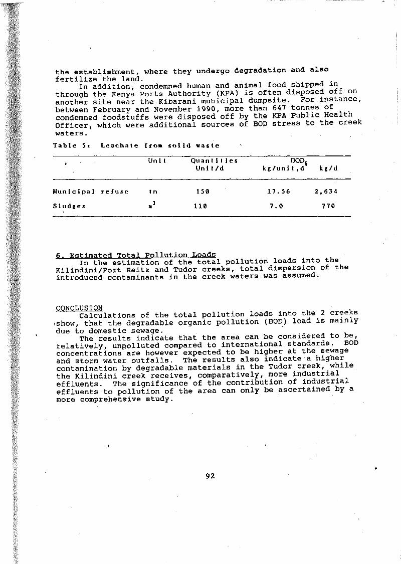
the establishment, where they undergo degradation and also fertilize the land. .In addition, condemned human and animal food shipped through the Kenya Ports Authority (KPA) is often disposed off on another site near the Kibarani municipal dumpsite. For instance, between February and November 1990, more than 647 tonnes of condemned foodstuffs were disposed off by the KPA Public Health Officer, which were additional sources of BOD stress to the creek waters.Table 5t Leachate ( t o m solid vaste
1 Uni 1 Qu a n t i 1 i e s Uni t/d
BODj kg/uni t,d kg/d
Municipal refuse t n 150 17.56 2,634
Sludges n.3 110 7.0 770
6. Estimated Total Pollution LoadsIn the estimation of the total pollution loads into the Kilindini/Port Reitz and Tudor creeks, total dispersion of the introduced contaminants in the creek waters was assumed.
CONCLUSION ^ ,Calculations of the total pollution loads into the 2 creeks ishow, that the degradable organic pollution (BOD) load is mainlydue to domestic sewage.The results indicate that the area can be considered to be, relatively, unpolluted compared to international standards. BOD concentrations are however expected to be higher at the sewage and storm water outfalls. The results also indicate a higher contamination by degradable materials in the Tudor creek, while the Kilindini creek receives, comparatively, more industrial effluents. The significance of the contribution of industrial effluents to pollution of the area can only be ascertained by a more comprehensive study.
92
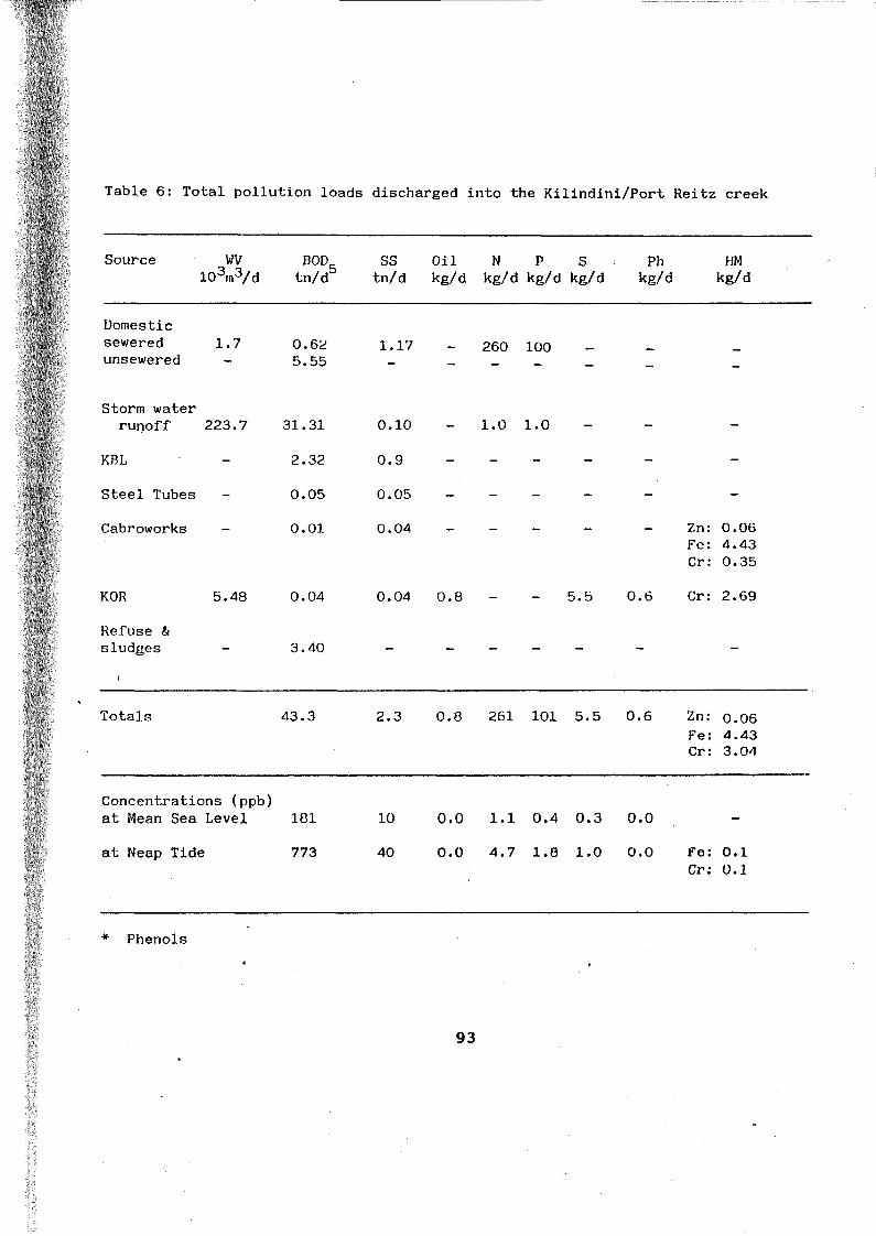
Table 6: Total pollution loads discharged into the Kilindini/Port Reitz creek
Source WV103rn3/d
BODtn/d
SStn/d
Oil kg/d
N P S kg/d kg/d kg/d
Ph kg/d
HM kg/d
Domestic sewered 1.7 unsewered -
0.625.55
1.17 - 260 100 - - -
Storm waterrunoff 223.7 31.31 0.10 _ 1.0 1.0 — — -
KBL 2.32 0.9 - - - - - -
Steel Tubes 0.05 0.05 - - - - - -
Cabroworks - 0.01 0.04 — — — — — Zn: 0.06 Fe: 4.43 Cr: 0.35
KOR 5.48 0.04 0.04 0.8 - - 5.5 0.6 Cr: 2.69
Refuse & sludges - 3.40 - - - - - - -
Totals 43.3 2.3 0.8 261 101 5.5 0.6 Zn: 0.06 Fe: 4.43 Cr: 3.04
Concentrations (ppb) at Mean Sea Level 181 10 0.0 1.1 0.4 0.3 0.0 —
at Neap Tide 773 40 0.0 4.7 1.8 1.0 0.0 Fe: 0.1 Cr: 0.1
* Phenols
93

Table 7: Total pollution loads discharged into the Tudor creek
Source WV 10 m3/d
BODtn/d
SStn/d
Oilskg/d
Nkg/d
Pkg/d
Domestic sewered 25.92 unsewered -
3.115.55
11.76 - 1.680 420
Storm water runoff 223.7 31.31 0.1 - 1.0 1.0
KMC slaughterhouse — 0.47 0.44 170 - -
Totals 39.18 12.3 170 1.681 421
Concentrations (ppb) at Mean Sea Level 455 140 2.0 19.5 4.9
at Neap Tide 1633 510 7.1 70.0 17.5
r
ReferencesGovernment of Kenya (GOK) (1988). Tourism market 1987/88.
Ministry of Tourism and Wildlife. 45p.GOK (1977). Mombasa water pollution and waste disposal study.
Marine Investigations VI. Ministry of Local Government. Norconsult A.S.
GOK (1974). Mombasa water pollution and waste disposal study. Draft Report. Ministry of Local Government. Norconsult
A.S.Iwugo K. 0. (1990). Basic concepts of environmental quality
control in relation to baseline studies on land-based sources of pollution. Introductory lecture. 30p.
WHO (1989). Management and control of the environment. World Health Organization. 153p.
94

KEyî*.im|«|lnjj sUDoni Mflngrov« »wump Conil n«f I Cotiü« way In 0 u 9 trliil a r ta
/rfy/n itihlMl!••• r/>i
IOMBASA
p|««.rn I. Ot II,n „tmly »rm,, »l.owl„w „nmp|,„„
95
*

Septic Tank Soakage PitsPit Latrines (No marks)
WEST MAINLAND
® aCre a ,med
ChangamweKipevu
it- CHANGAMWE TREATMENT
PLANT %
\
Kibarani
T U O O R C R E E K
Mahupa J.■yMTONGWE
LlkonlI»«Perry NORTH MAINLAND
momoasISLAND
TREATMENT PLANT
2 Km
Figuro 2s Sewage disposal systems sourcet GOK (1974)
96

Drained Area•ViiV\vll\W
WEST MAINLAND•o
I-:--.- ,-j/■ % • a * * ■-Í »14 hg*^w«
/'.'•V" • *N»t• • ; .i I. • . 'A
I
Q
NORTH MAINLAND
SOUTH MAINLAND
NYALI
2 Km
Figure 3»< Existing storm er drainage souront GOK (19/ I
drainage areas
97

/ 4 6 8 74.2.4.2. Monitoring Qf Pollution levels in the coastal and
estuarine environment around MombasaBy : J.Wijnant, K.Delbeke, J.Munga, S.Mwangi, M.Owili. With technical assistance of M.Umani,J.Othoto, N.Marocco and P. Mathendu
INTRODUCTIONThe study is done in collaboration with the Kenyan Government
Chemistry Department and is supported by UNEP, in the frame of the EAF/6 program "Assessment and Control of pollution of the Kenyan Marine environment".The theoretical investigation of the pollution loads in the creeks around Mombasa (see previous chapter) indicated that Tudor Creek receives essentially biodegradable organic pollutants from municipal sewage andstormwater drain outfalls. Kilindini/Port Reitz creeks receives less pollution from municipal sewage but is also polluted, to an unknown extent, by industrial pollution and leakage from the Municipal dumpsite.The pollution monitoring part of the program will allow one to obtain a set of baseline data to be compared with the obtained results from the theoretical investigation and to be used as a reference for further pollution monitoring.At present, basic environmental parameters are being investigated ¡Salinity, Temperature, PH, Dissolved oxygen, Nutrients, Particulate organic carbon, BOD5 , petroleum hydrocarbons, heterotroph and pathogenic bacterial counts and phytoplankton biomasslevels. The data will allow us to have a first general evaluation of the state of the marine environment. In a later stage, environmentally toxic and stable pollutants such as
i organochlorine residues and heavy metals, will be investigated. This report deals with the first set of data obtained in the Mombasa Creeks.MATERIALS AND METHODSWater (surface and bottom) and sediment samples were taken on board of the RV Maumba with respectively Niskin bottles and a Van Veen grab sampler. The samples were collected at different stations in Kilindini/Port Reitz Creek, Tudor Creek and Gazi (reference site)(Fig.1) between 10th April and 17.th May 1991. At the connection between Makupa end Kilindini (oilspill and municipal dumpsite) and at Mbaraki (stormwater drainage outfall) samples were taken at different time intervals during one tidal cycle.Salinity, temperature, PH and water depth were measured immediately, using the respective meters. Water (1 liter) was filtered immediately on board for measurements of chlorophyll and POC. The filters were preserved through freezing before analyses on a spectrophotometer, according to Parson and Strickland. Nu
98

trients are preserved with chloroform before freezing and analyzed with a nutrient analyzing system. Petroleum hydrocarbons were extracted on board and analyzed with a UV spectrophotometer. Oxygen and BOD5 values are obtained using the Winkler Method. The method used for heterotrophic and pathogenic bacterial counts are described in Wijnant et. al .. 1991. All samples are taken in duplicate, except for bacterial countings, BOD measurements and oxygen levels, which are taken in triplicate or more.
RESULTS AND DISCUSSIONTable 1 gives an overview of the results obtained sofar. The data on POC, nutrients and petroleum hydrocarbons are being processed and will be available soon.The differences noted in temperature between the different station are a reflection of the onset of the rainy season during the sampling period. No clear differences in water temperature were noted between the different station within one transect, nor within one tidal cycle (for Makupa and Mbaraki sites).Pfr values range usually range between 7.7 and 8.5 between. The lowest value was recorded in Gazi (7.3), the highest pH in Makupa(9.4). Surface sea water has a characteristic pH range between 8 and 8.3. A change in pH due to photosynthetic uptake of carbondioxide by phytoplankton to 9.5 and a decrease to 7.3 at night are still to be considered as normal for biological active Marine tropical waters. The pH values therefore do not seem to cause any hazard to the marine environment.Low oxygen values are sometimes note. Oxygen values range between 4.5 and 9 mg/1. Values below 5mg/l were recorded for the deeper water layer during outgoing tide for the Makupa site and for the whole water column, at the Kenyan meat factory .Relatively high BOD5 ,heterotrophic biomass and Ecoli numbers are recorded for the Makupa area and Tudor Creek (Coast General),
i When considering the WHO (1967) guidelines of lOOO/lOOml for total coliform group and the EEC guidelines (1975) of 500 total coliform and/or 100 faecal coliform/lOOml, than one can note that all levels are under the guidelines.When considering the data on oxygen, B0D5, bacterial numbers and chlorophyll levels in some more details (Fig 2 - 4), one observes for the surface water in Kilindini Creek a decrease in oxygen and an increase in chlorophyll levels and B0D5 levels going inward in the creek, (fig 2). A decrease in oxygen level and an increase in chlorophyll, BOD* levels and heterotrophic bacterial numbers was observed with outgoing tide, compared to incoming tide, for the surface waters of the makupa site (fig 3). One must therefore consider Makupa creek as an important source of organic pollution for Kilindini creek, due to the Kibarani dumpsite and the remains of the oilspill.The deeper water samples from Kilindini Creek show a similar decrease in oxygen levels as surface waters, however with sometimes lower BOD levels and heterotrophic bacterial numbers in
99

the Makupa area (fig. 2). The bottom water samples from Makupa show lower levels of oxygen, BOD, and heterotrophic bacterial numbers at outgoing tide,compared to incoming tide (fig 3). The decrease in oxygen as well as in heterotrophic bacterial numbers and biomass levels for the bottom samples compared to the surface water samples in the Makupa area should be investigated more deeply.The samples taken at Mbaraki only show small changes in oxygen, B0D5 and heterotrophic bacterial numbers over one tidal cycle (fig 3). Mbaraki is therefore, at present, not considered as a major pollution site for Kilindini Creek.In Tudor Creek, a lower oxygen and higher B0D5, chlorophyll and bacterial levels are observed for the inner creek, at the Kenyan meat factory compared to the open sea station (fig 4 ). The samples from the hospital are contradictory, showing either normal or elevated levels for BOD, and heterotrophic bacteria (fig 4) as well as for E coli (table 1).When comparing the data with the ones obtained for Gazi, similar environmental data are observed. The measured BOD5 values are however much higher then predicted from the preliminary theoretical investigation (Table 2) . More replicas are however needed and a remeasurement of the contamination levels (data from 1975) at the sewage and water drainage outfalls seems necessary and is being undertaken .
CONCLUSIONThe monitoring of pollution levels in the creeks around Mombasa has started, the first data are available. The first results, although preliminary, are higher than the ones obtained in the 'theoretical investigation. The area shows a minor pollution by organic degradable compounds. The area around Makupa is probably to be considered as the most important pollution source for the area. The area around the Coast general hospital also surely- needs further investigations. Further data collections will allow one to obtain a reliable database, including variations due to tidal water movements and seasons. The results on other basic parameters and on important toxic com pounds wii1 allow us to make real conclusions.
Table 2 : BOD5 values obtained through the theoretical investigation and the monitoring study(mg 02 /m3) Area BOD5 calculated BOD5 measured
Mean Max Mean MaxKilindini 181 773 1200 1720Tudor 455 1633 973 1600

6 E C C e e c c
o o © o n oo o o o© d e e c c
0 o<t d d ©1 io oM © -• d
4JC<UM(1)<WMH•H
0)xi*P
id■H s«J Xn Idsr— 1m4-1 cC •rH<u secO -HM N•r- 10t> ÜcdJ C•HT»(U TJM C3 10m•d 100) wB <0m BO oSd)tr>TJG Ciid 0« oM• • IÜrH (0d)rXrH (DXi d)10 MEh ü
DOOo
©©<co
©E
©OO
o oo oo <1 o o o o-4 1 o o <J ot O Cl ci -4 Mo © 1 1 1 t© *-* o o o o
o o© CD
O_ <t O © o 4 ©4 4 I ©I I o •O O 4 0
o o© © o od d O o o ©t 1o o ci d Cl d 1 1t !© o o o o o-» M ci d © Cl
O O o o-4 4 © O4 4 ~4 (D
Od O0 *«H ©1 IO oO 4 © ©
0 o ® 4 ©1 iO O © O n n
0 oh* © © ©1 io o © © o n
d ci r~
4 d ©© © i t© M N CT M -#
O © © ©
O o0 ©© 41 (O o o o © «o
o o0 od ©1 t (M © 4 ©
O O4 © © d « I O O .o ©d H
o©M
0 © ©1Oo©
N <* on o © n © © o o Cl © o\ © © 1 1 © Nt t N C- © © N © c- © O!E Cl © Cl -• h- © © -d 1 1 O) © 1 1© o f
oMo IO © © © © © © © © 4 © ©
m o o o © © —i 0) o o • o
« a « c* »«4 -1 <i 4 0) © © <1 c- d •-4d d d d Ci ci d d d 1
• d d© © o o o © o o 1 l«lo © o*J 0> 0) o ^ © 4 O Cl N o
< N N d d Cl N d d d d N
d 4 n ci ci ci d d d ci 4 © •40) m © <T> © © © © © © © © ©O »-4 *4 M *■» «-4 ¿ o © O c. © <1
E ?H © © © © © © © © N © N N N
© o © © 4 © 4 o Ci o o o ©< -4 O 0> © •■4 «-4 © N © © © © ©r»î d d N CI d d d d d ci d d d
© d N © N © ci © © © © © ©0,jr o o © © a) © © © © © N N NioH d d N d ci d d d d d d d d
XH © o © o © O © o © û © o ©n.td Ho J
* B© M ©
M ■>4*> 4->
c M c _ Mz •*4 •>4 C •V4 M — Co H n. © ••4 V
a m c B c u t. B1- 3 u *p4 O «4 o O 0 w>4< .* 4 •— O M © © 0 Mf- 4 £> •*4 c m4 3 3 C Bin n C •#4 M f- J f- -4 O
101
200-
1000

iVr:rs/,T« «for
Sam pling stations * M an g ro ve sw am p f i Coral He® I C ous« w ay Industrial area m m
Mmm an oce*H»Me
0MBA5ASlAND 3TORT REITZ
%>
figure 1« Map of the study area, showing sampling stations
102

oM
«J
ILJEa KI*.O
+
oO0
o
K mo md O
ü O e m
(spuosnoMx)»x’woie'zoooe(epuDsnom)
»xnoie'zo'aoe
oK>oI)oo.o o o o o o
EE.e =5 _2® 2 g o 5 ?3 N — i " ° M
2c•*a«•
1
aiai§
ï~ «n o
r—irH 4J>4 CJC CUa »-c0 CUm 440 44•H -<4 • •JC x)u en
01'4J 4Jid •d
en■h eneu M tn> eu C(D XI -H —H H gdlJl 3 OiCn C Ë H (Ö I
inQO«
CO UD I* • vû
Cnn•H Mp4eucu
c:■r4
(d •H U, -CU en 4->H O d) (d> XI cu
r“t U•H
C XI Ul T)cu a — c tr> o -H>4 M ,X r-4X -P CU -Ho o ai «M M d) CJ - 4-1 tH CU -Hen x: C a -hO H - d•h «d c:4J 4-1 --H (d O h eo ■H 4J -H tH
M « rd T}> C G M (d *H •HM Ul Ul C rH C ’Heu cu o t } m > -m c3 CU 4-> H tn »—i <d 1—i •H 4J -HPm (d w ui
enent-HII
(spuDsriOi<j)H K 'G O O l .u J v « M » ;â * ( o i 4 ç- i u / 6 u i ) j o * ( Î « ^ / O ^ K O O G lo 3
(■puosnoqj.)i“Voooi .ujujoiano i ,rLu/6m)2o:(rul/o6lJJ>saoQ

e—' x^ a
oM© o*o'o ©* e e O«e n«3c»o»o r»o oo e
(»»■»oineui)♦ o y . , u » .* J ‘5 | f l : ( o i * ç u i * / 6 u # ) 2 O i< C ü ' / D f t ^u ) 9 O O 0
(ipUOin«l|¿) ftfti (pv'.'.'Â.'iOifl'.ÎOl ,çi.ti /fty
CD S^ 3
«« K « n o
h 9
(•pueanetij.)®X‘f1O10‘2O*OOO («puovnoMi)»x'itoin'so'oos
I OL(
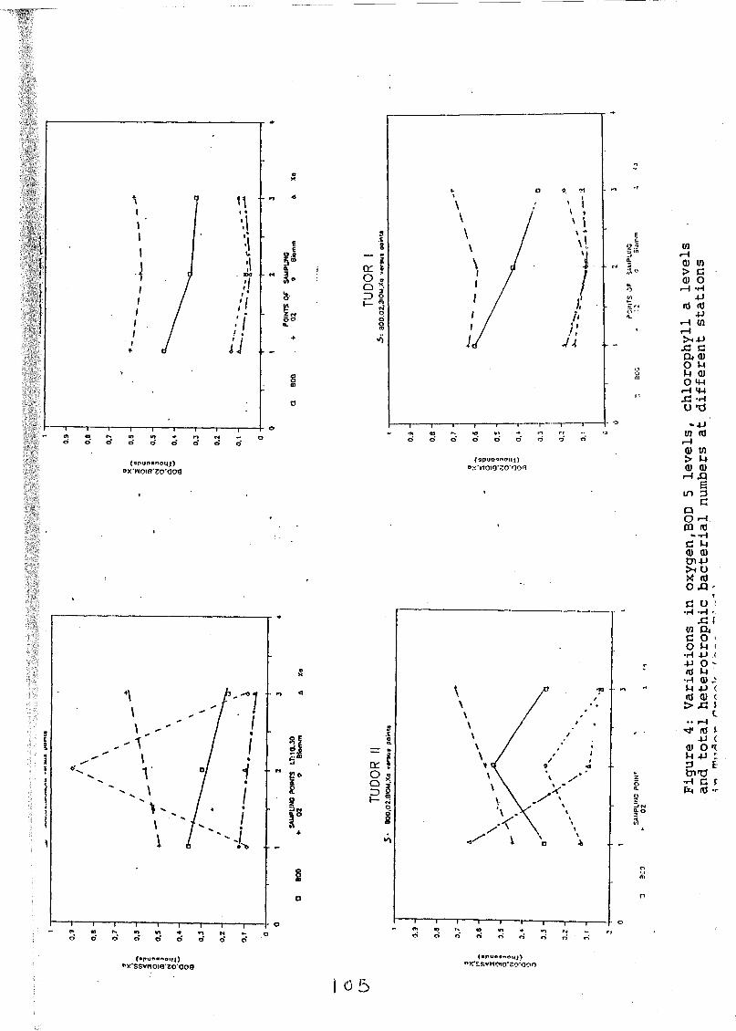
t
r«*om
(spuf»«not|_t)©X'WO!0'£O*OO0
(spuonnotix)ox'wotg'o'no«?
sc%
I
>i\
0 0 ry O
O E2eSíg-6*s
s?? «
s.Eoa.«i>
Q 5O s f- °1-“ Noo8
fh 0 0 r*
{•pua«noi||)î>X‘SSV«OIQ2O'OO0
i 0 5
(•pueinotij)nX*£RVHO»0‘no‘OOO
mi—id) ín> c0) o
»—I -HP(d (d■M
•H Ulf—(>14J
43 Ca, <uO MM d)O 4-1
.-H 4-143 -hU 13
-pui (d1—1d) Ul> Md) <u-H -Q
Bin ¡3
CQO iCD (d
— -rid Md) d)tnptu oX idO 43 *
td o I•H *H
X fUl cud o (O M (•H 4-> (-U o *-(d M•H d) 1U P 7(d d) (> 43 *
C•* f—1
rd i.44 cd) o a
M Pd ttPT)•h d cfrr rd •r

/ 4 6 8 84.2.4.3. Assessment of pollution impact on the Mangrove Oyster,
ment of the impact of pollution on the Mangrove oyster.Crassostrea cucullata By: K.Delbeke, O.Omolo, M.Umani & O.Anyango
INTRODUCTIONThe pollution impact study is part of a collaboration programme "Assessment and control of pollution in the Kenyan coastal and marine environment". The programme is conducted as a collaboration between KMFRI,Government chemistry and KBP. It consists of different subprojects:(1) A theoretical investigation of the pollution sources and pollution loads from municipal, industrial and agricultural wastes (see previous chapter).(2) Monitoring of pollution levels and establishment of baseline contamination levels for the area(see previous chapter).(3) Assessment of the effects of the pollution on the marine
venvironment(this study).It is aimed, in the frame of the third subproject, to investigate the biological condition of the Mangrove oysterf Crassostrea cucullata. from the potentially more polluted area (Mombasa), in comparison with an "unpolluted" site (Gazi). The Mangrove oyster,was chosen as indicator organism, due to the known usefulness of bivalves as indicator organisms (e.g.Phillips,1980; Bayne et.al.,1982; MAP,1987;), due to the importance of the oysters for human consumption and due to available knowledge of the oysters' biology and ecology (Ruwa 1984 and 1990; Tack et.al., 1990).The study consists of three parts :- study of the basic biological characteristics (size frequency
i distributions, condition and sexual maturity)'.- study of the biochemical characteristics (lipid and protein content, enzyme activities)- study of the physiological characteristics (metabolic and grazing rates, scope for growth)This report only deals with the first part of the study.
MATERIALS AND METHODSBetween 20th and 30th March 1990 (pre-spawning and spawning period), oysters were collected respectively in Gazi Creek (40 km south of Mombasa), Mtongwe ( Kilindini creek) and Port Reitz (Fig.l). Due to the known impact of the population density on the substrate and of the tidal height of the oysters1 site on the growth of the oysters, only individuals being characterized by less than 70% cover on the substrate and situated at a tidal height around 60-95 cm above datum were collected. The collected oysters were immediately transported to the laboratory and frozen alive. The shell sizes, sexual maturity of the females ( size of
106

gonads and ripeness of the ova) and the dry weight of the oysters were recorded.
RESULTSThe results on the oysters' shell size (length and width) and the oysters' dry weight (Table 1 and Figs. 2 & 3) show that the oysters from Gazi are smaller than the oysters from Kilindini (Mtongwe) and Port Reitz. The noted differences for shell length and dry weight measurements are significant (P 0.01 in a students t test).When comparing the oysters' ratio : dry weight oyster/shell length, being an indication for the oysters' condition, one observes the highest condition index in Mtongwe. The oysters from Gazi have the lowest condition index. The noted differences are statistically significant (P 0.01 in a students t test).The observed differences in shell sizes, body dry weight and condition index are not to be understood by differences in maturity stages between the 3 populations (table 1) nor by 'differences in population densities or tidal height (see materials and methods).The comparison of the condition index also excludes possible differences in oysters size due to collection of the oysters (essentially the bigger ones) for human consumption.
DISCUSSIONThis first preliminary investigation could not detect any adverse effect of pollution from the Mombasa district on the considered oysters' growth. The area around Mombasa is essentially characterized by pollution by biodegradable organic compounds from municipal discharges and some additional industrial pollution of yet unknown magnitude (see previous chapter). It therefore seems possible that the increased load of organic matter might enhances the oysters' growth, directly (uptake of DOM or POM by oysters) or indirectly (through eutrophication). The results are nevertheless to be interpreted with care. More data on population sizes, and condition index (as internal shell volume) are needed. The study of the biochemical and physiological characteristics of the oysters as well as the analyses of contaminants in the oysters' tissues will allow us to draw conclusions on the oysters condition and its value for human consumption.
107
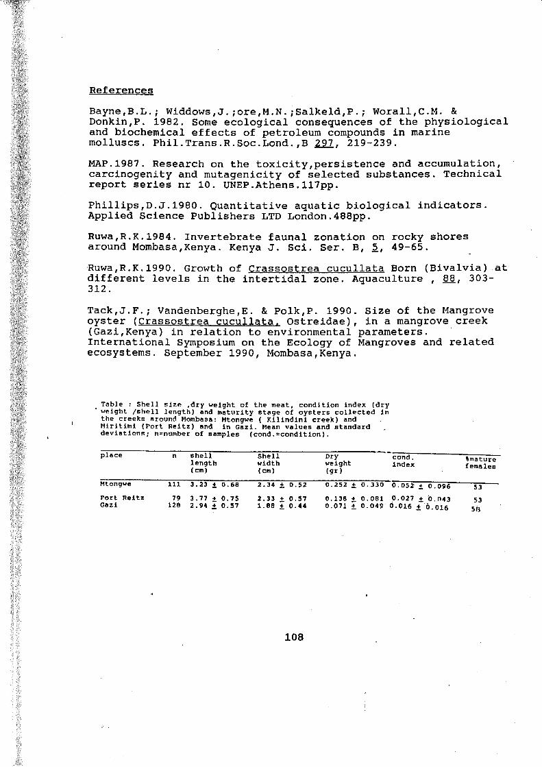
ReferencesBayne,B.L.; Widdows,J .; ore,M.N .;Salkeld,P.; Worall,C.M. &Donkin,P. 1982. Some ecological consequences of the physiological and biochemical effects of petroleum compounds in marine molluscs. Phil.Trans.R.Soc.Lond..B 297. 219-239.MAP.1987. Research on the toxicitypersistence and accumulation, carcinogenity and mutagenicity of selected substances. Technical report series nr 10. UNEP.Athens.117pp.Phillips,D .J.1980. Quantitative aquatic biological indicators. Applied Science Publishers LTD London.488pp.Ruwa,R.K.1984. Invertebrate faunal zonation on rocky shores around Mombasa,Kenya. Kenya J. Sei. Ser. B, 5, 49-65.Ruwa,R.K.1990. Growth of Crassostrea cucullata Born (Bivalvia) at different levels in the intertidal zone. Aquaculture , 88, 303- 312.Tack,J.F.; Vandenberghe,E. & Polk,P. 1990. Size of the Mangrove oyster (Crassostrea cucullata. Ostreidae), in a mangrove creek (Gazi,Kenya) in relation to environmental parameters. International Symposium on the Ecology of Mangroves and related ecosystems. September 1990, Mombasa,Kenya.
Table : Shell size ,dry weight of the meat, condition Index (dry weight /shell length) and maturity stage of oysters collected In the creeks around Mombasa: Mtongwe ( Kilindini creek) and Mlrltiml (Port Reitz) and in Gazi. Mean values and standard deviations; n=number of samples (cond.»condition).
place n shelllength(cm)
Shellwidth(cm)
Dryweight(gr)
cond. index %mature
females
Mtongwe 111 3.23 ¿ 0.68 2.34 ± 0.52 0.252 ± 0. 330 0.052 4 0.096 53Port Reitz 79 3.77 + 0.75 2.33 + 0.57 0.138 + 0.081 0.027 4 0.04 3 53Gazi 128 2.94 ± 0.57 1.88 4 0.44 0.071 4 0.049 0.016 4 Ö.016 50
108

Sam pling stations # M angrove sw am p jR
Industrial arca
Mlw*p* /nido'
mmIHWM* OCCAM» 30 C * 30 'S
^T'Orne
5 MOMBASA rPORT REITZ tí ISLAND
‘V ’ is
Figuro 1: Map of the study area, showing sampling stations
109

Ni.
4035-3025-
20-
15-
10-5-
0
MTONGWE
N11
05 0-10 0
—j j ^Ü~Ô20 0-25 0 30 035 0 40 0 4 5 0 50 0 55 0-60 0 65 0-70 0-75 dfy weighKgr)
25
2015-
10
5-1
M I R IT I NI
P P O UN 8 ° e; k
50
40-130
20-
10-
p p p 2 p ° p p èsSfi.Q O i I O W U ldry weight (gr)
G A Z I
P8J í h r >) p p p p op p p £ l > p £> p A ç> 1§ tí « 55 iá tà g g g æ £ dry weight (gr)
Figure 1: Frequency distribution of the dry weight of oysters collected in respectively Mtongwe, Miritimi and Gazi.
110

N
Figure
35
3 0 i
25
20 15
10-
5 -
0
MTONGWE
-n— r- t=J-MIRIT IN1
25
20 15 H
10
5
0N
50
4 5 -
4 0 -
35 -
3 0 -
2 5 -
20 15
10 S
0
- i r r -
GAZI
0 5 1 0 15 2 0 25 3 0 3 5 4 0 4 5 5 0 5 5 Shell length (c m).
2: Frequency distribution of'the shell length of oysters collected in respectively Mtongwe, Miritimi and Gazi.
Ill4

4 6 8 94.2.5. A report on the culture of Siganus sutor in tanks.
B y : B .Okoth
AIM.1 The aim of this project is to try different Culture techniques so that these fish can be can be successfully
Cultured here in Kenya; as they are very popular and their market value is within the reach of the common man.
2 To try and formulate cheap and adequate diets formulated using local Ingredients growth and good body Composition.
3 To try and Induce these fish to spawn in captivity as theavailability of seed is of a major constraint in agriculture. So far no such research is going on in Kenya(for Marine fish) and it is important that it is done so as to promote aquaculture given the vast area of sea that Kenya has.
V
METHODOLOGYFish are normally brought in live from Gazi, where they are
caught during low tide by beach Seining. The fish caught are then packet in polythene bags containing little sea water and thebag is then filled with oxygen and lied.
These fish are then transported to the lab where they are kept in 1 ton concrete tanks. In the 1st week the fish are fed on algae collected from the sea and in the second when the fish are used to tank conditions they are trained to eat pellets.
Different types of pellets have been composed so far, and experiments are going on to find the suitability of these proteins. Experiment are also being carried out to find the optimum protein and fat requirement of these fish so as to help
, in compounding pellets that meet the nutritional requirement of the fish.
This work is still in the early stages.
CONSTRAINT1 The biggest constraint has been the availability of sea
water but this now has been rectified by the acquisition of a new pump.
2 Lack of aquariums is also another problem. These are required for larval rearing we need 20 30L plastic aquariums for stocking larvae. The experiments have to be done under different environmental conditions as well as different feeding regimes.
112
4.3. RESEARCH DONE BY VISITING SCIENTISTS
Report study trip to Mombasa - Kenya. November 12 - 18, 1990.Dr. Maya Borel BestNat. Mus. Nat. Hist. LeidenPostbus 95172300 RA Leiden, the Netherlands.
Purpose: One week orientation on possibilities of coral reef research projects in Mombasa - Kenya.
Introduction.As teacher of the coral reef ecology course (FAME) in the VUBrussels, I was asked to supervise the MSc student Amanuel Melles from Asmara-Ethiopia. Coral reefs are worldwide threatened by overexploitation and landerosion. The research proposal of A.Melles is therefor orientated towards "the influence of terrigenous sediments on health and growth of coral reefs off the Kenyan coast".Because I was not as yet familiar with the coral reefs off Kenya or with the practical circumstances to carry out a project there, I was asked by Prof. P. Polk to do some orientating fieldwork in Kenya with A.Melles in November 1990. One week work with some fieldtrips should be enough for orientation in view of my twenty years experience with coral reef research in the Indo-Pacific (mainly Indonesia) region.
KMFRI = Kenyan Marine Fisheries and Research Institute - Mombasa.' The research station is well situated along the sea side in Mombasa, but has to contend with many reorganisation problems. The director Dr. E. Oktmwa was very helpful and hospitable and promised the reef team, consisting of A. Melles, J. Mutere, two Belgium divers (M.Maas and D.Martens) and myself, to supply the transport (jeep and boat) necessary for fieldwork.The technical services and material of car and boat, as well as available diving equipment were not adequate for this kind of research. The main problems concerned the diving equipment and boat (dingy). For safety reasons a well functioning compressor and regular tested SCUBA-tanks are essential. This was not the case however, so diving with borrowed tanks and bad air was the result. Most work therefor was done by snorkling.The boat transport was not sufficient either, the motor broke down and the light boat tipped over with a little swell on our way to the reef at Gazi. In conclusion I can state that the KMFRI equipment for reef research is not adequate as yet . Good reliable diving equipment and’ a heavier motor boat is necessary for further coastal reef research.
KMFRI Guesthouse. FAME project.Under the guidance of Prof. P. Polk the KMFRI guesthouse is operating well. Scientists and students are invited to participate in marine and fresh water projects.As a consequence of the in 1988 started theoretical reefcourse "Coral Reef Ecology" as given in Brussels for FAME students, the plan has risen to start fieldwork possibilities for the students in Mombasa and eventually to give the FAME course also here. 1 1 3

Kenyan reefs.Coral reefs are complex ecosystems characterized by a state of dynamic equilibrium comprising innumerable invertebrate fauna and flora. Healthy reefs are important for a rich marine life and for protection of the coast. The equilibrium is subjected to the impact of sediment flow. Currents and fresh water imputs from rivers deliver sediments which have an important controlling effect on the reefs. The Kenyan coastline extends over 450 km along East Africa. The continental shelf is narrow and supports fringing reefs and patch reefs which lie o.5 - 2 km offshore.During the excursions made to reefs north of Mombasa, Malindi and Gazi, the general condition of the reefstructure and the diversity of the coral species (main reef builders) composition, was studied.In the lagoon and innerreef algae and seagrass beds dominated first to be taken over by low diversity reef patches. Approximately 60 coral species belonging to 22 genera were counted. An inventarisation was made and a reference collection was started.Striking was the absence of coral species that indicate healthy and rich reef biotopes. Also the large colonies of Porites (up to 4 m diameter) were, for a large part dead and showed only living parts at the outsides, the toppart was covered by sediment and dead.It was my conclusion that these inner reefs along the coast of Kenya are strongly influenced by land erosion (sediment - fresh water), but also by the effects of too heavy touristic pressure.This will be tested by the work of Amanuel Melles of which the practical part has started in November 1990 and will be worked out during the next six months in the i» tía* Netherlands under my guidance (see Research Project Proposal A. Melles Oktober, 1990)
Conclusions.'To start a coral reef research programme in Mombasa for- East Africa the practical infrastructure in the KMFRI has to be installed.Because the inner reefs along the coast of Kenya are strongly deteriorating a reef programme should be set up, that is orientated towards reef protection. The most important destructing factors (probably sediment, river outlet, tourism) should be studied in order to advise the Kenyan governe- ment of the necessary steps to be taken to save the coastal reefs from complete destruction. Because the reef construction and diversity of the outer reefs are far more solid and rich, the recolonisation of reef building organisms at the inner reef might take place in the future when the destructive factors are reduced as far as possible.
114

REPORT OF M.Sc. DATA COLLECTION FIELD WORK ALONG THE KENYAN COAST
Amanuel Melles M.F.A.M.E. Lab Ecol VUB BrusselsTowards the partial fulfillment of my M.Sc. I did my field work along the Kenyan coast during-November 1990. The field work was carried out at several sites on the Kenyan coast. Preliminary survey of the following sites was made: Kenyatta Beach, Bamburi,Nyali, Malindi and Gazi. The survey of the latter site ended in failure due to a boat accident. Most of the preliminary surveys were done by snorkeling and covered the first week of November. After the selection of sites, corals were collected for taxonomic, isotopic and radiographic studies. The depth regimes éovered during collection ranged from 2m up to 23 m.Preparation of coral samples for studies (cleaning, labelling, etc.) was done at the KMFRI guest house. For isotopic and radiographic studies coral cores and slabs are needed: in the absence of a corer, every attempt to improvise at the KMFRI’s workshop did not bear fruits. Corals slabs were roughly prepared with the help of stone disc cutting machine at a local workshop in Mombasa. Precision cutting will be done in Amsterdam.Spot X.rays of some coral species were taken.Apart from coral collection, line transects were laid at Malindi and quadrants at Nyali and Bamburi. By this method coral species coverage was estimated.In order top aid in the identification and characterization of
, coral species and bottom topography, slide pictures were taken using a Nikonos underwater camera.For a possible long term monitoring of coral reef, permanent site wás established comprising three depth regimes (12-17m).During my field work, I was assisted by my advisor Dr. Best.Dirk Martens, Mare Maes and Erik Slim, to whom I am grateful, have joined me during my diving sessions and helped considerably in underwater sampling tasks.I had encountered some logistic problems and inconveniences. Against all my expectations, cooperation with M s . J. Mutere proved: difficult, if not impossible. My passport has been withhold for two weeks by the Malindi Wildlife Service Warden because the presumed papers of permission were either delayed of missing.On Nov. 14 1990, I had an accident while I was out at sea near Chale Island, Gazi Dr. Best, J. Mutere and Erik Slim and the boat skipper were with me. The accident occurred when the engine of
115

the boat stopped functioning, and moments later we were overturned by big waves. I have lost an NC-11 diving computer, a Nikonos compact camera and a pair of glasses, J. Mutere lost one of her fins. Local fishermen helped in towing us towards the coast. Although such accidents can happen, the KMFRI's boat was not sea-worthy at all, especially in the outer reef.In accomplishing my task, my work was facilitated by the help of Prof Polk and Dr. K. Delbeke. I extend my thank to both Erik Slim, apart from joining me in the later and deeper dives, had assisted with transportation. My special thank to him whenever possible, I took the opportunity if my stay in Mombasa doing a literature reach through RECOSCIX WIO . Mr. P. Pissierssens was helpful in thin regard.My field work was made possible by the financial assistance provided be Sarec, Roata and VLIR and efforts of FAME. I am grateful to all. KMFRI Cooperation is also acknowledgedMy field work was made possible by the financial assistance provided by SAREC, ROSTA and the VLIR project and efforts of F.A.M.E. I am grateful to all KMFRI's cooperation is also acknowledged.
liu

fiterim ifytat HarpGctbúiéa
4691Kenya-Belgium Project in Marine Sciences
"Higher Institute for Marine Sciences" KMFRI - VLIR project
Marine phytal Harpacticoida from Kenyaw ith emphasis on seagrass dwelling species
by Bruno Demeulenaere
Introduction.
In the framework of the Kenya-Belgium project in Marine Sciences and the KMFRI - VLIR project, a prelim inary study of the phytal harpacticoids of the Kenyan coast was undertaken.
The aim of this work is, in firs t instance, to provide an introduction to tlie species of phytal harpacticoids from the region as well as to present data on abundance and diversity of this particularly interesting component of the meiofauna. The animals were obtained from seagrasses and algae but the emphasis is put on seagrass (Thalassodendron sp.) dwelling species.> To (re)evaluate the hypothesis that harpacticoids can be used as a “fine tool” in pollution monitoring (see also Heip, I960), the diversity of harpacticoids from two places along the Kenyan coast w ill be compared among each other and also w ith the respective nematode/copepod ratio's (further refered to as N/C ratio) of the two sites. The N/C ratio is widely accepted as being a reflection of the condition of a system w ith regard to pollution stress, although it is designed to be used for sediment dwelling species.
A brief discussion about the usefulness of d ifferent diversity indices, by evaluation of the present results and comparison w itti earlier (and more extensive) studies of this kind is presented.
On the species lists also a TWINSPAN analysis is performed to gain some additional knowledge on the respective assemblages of harpacticoids. ,
Next to tile diversity analysis, harpacticoid abundance w ill be determined.
A second part of the present work is dedicated to taxonomy. Results are too prelim inary to give an account of them in this report.
117

M a r im p b jta l H a rp rx th ú i6a
M aterial and methods.
The study area
In order to estimate the abundance and diversity of harpacticoids on seagrasses and to evaluate their possible use as a fine tool in pollution monitoring, samples were taken at two locations along the Kenyan coast English point (ref. “pollution") and Gazi (ref. “no pollution").
English point, the site that is considered to be under some environmental stress, is situated a t the mouth of Tudor Creek north of Mombasa Island. The samples are in fact not taken a t English point itself bu t in fron t of the little beach next to the Kenyan Marine and Fisheries Research Institute and very near to the actual point.
Gazi is a small fishing village some 50 km south of Mombasa. The samples that were taken there are considered to be representative for a nondisturbed site.
Material and methods
Only the leaves of the seagrass Thalassodendron sp. were considered. They were collected by gently sliding a transparent plastic core over one or (where possible) more leaves at a time .and then closing the core at both sides. The total content of the core is transfered to a plastic bag. One sample consists
■ of leaves taken from one plant or from plants in the near vicinity.A t English point 2 x 2 replicas were collected a t low tide (outgoing, 1 to
1/2 h before lowest tide). A t Gazi, 2 replicas were taken in the main tidal channel and 3 in the artific ia l channel facing the oyster racks ( see Fig. C ); also a t low tide (outgoing, 1 to 1/2 h before lowest tide).
In tlie field, MgC'l2 (IOS) was added to the leaves in the plastic bag which was then shaken thoroughly. MgCl2 serves to stun the harpacticoids present on the leaves. In the lab, the content of the plastic bags was poured over a 63 um sieve. Subsequently, the leaves were washed w ith a j% formaldehyde solution.
In order to have an idea of the effectiveness of the technique used to remove the animals, 5 leaves were picked out a t random to check them under tlie binocular (Wild). No harpacticoids were found on the rinsed seagrass leaves.
118
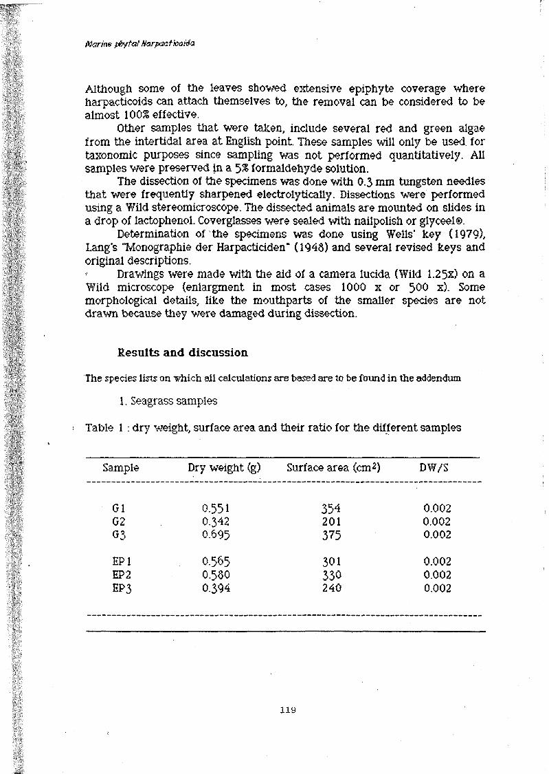
Marïm tfrftai Narp/Sütieoiéa
Although some of the leaves showed extensive epiphyte coverage where harpacticoids can attach themselves to, the removal can be considered to be almost 100$ effective.
Other samples that were taken, include several red and green algae from the intertidal area at English point. These samples w ill only be used, for taxonomic purposes since sampling was not performed quantitatively. A ll samples were preserved in a 5% formaldehyde solution.
The dissection of the specimens was done w ith 0.3 mm tungsten needles tha t were frequently sharpened electrolytically. Dissections were performed using a Wild stereomicroscope. The dissected animals are mounted on slides in a drop of lactophenol. Coverglasses were sealed w ith nailpolish or glyceel®.
Determination of the specimens was done using Wells' key ( 1979), Lang's "Monographie der Harpacticiden" (1948) and several revised keys and original descriptions.
Drawings were made w ith tlie aid of a camera lucida (Wild 1.25x) on a W ild microscope (enlargment in most cases 1000 x or 500 x). Some morphological details, like the mouthparts of the smaller species are not drawn because they were damaged during dissection.
Results and discussion
The species lists on 'yhich all calculations are based are to be found in the addendum
1. Seagrass samples
f Table 1 : dry weight, surface area and their ratio for the different samples
Sample Dry wTeight (g) Surface area (cm2) DW/S
G1 O.5 5 I 354 0.002G2 O.342 201 0.002G3 0.695 375 0.002
EP1 0.565 301 0.002EP2 0.580 330 0.002EP3 O.394 240 0.002
119

fifarim pbftal tiarpaGthoiéa
The equality of the DW/S ratio for all samples indicates that no big differences in epiphytic coverage occur. Differences in the number of species w ill most probably not be due to this factor.
2 Abundance and N/C ratio
Table 2 : numbers of Harpacticoida and Nematoda and their ratio
Sample Harpacticoida (ind./cm2) Nematoda (ind./cm2) N/C
G1 1.85 1.75 0.946G2 2.98 2.38 0.799G3 0.88 0.92 1.045
EP1 2.62 2.90 1.107EP2 2.69 2.83 1.052EP3 2.15 2.65 I .230
The fluctuating values for harpacticoid abundance in tlie Gazi samples are probably a reflection of differences in microspatial distribution patterns. Some leaves support much more harpacticoids than others. For example sample G2 w ith a surface area of 201 cm2 contained 2.98 ind./cm2 whereas
i sample G3, where the leaves have a surface area of 375 cm2- contains 'only' 0.88 ind./cm2. Note that these figures are nothing but a reflection of the abundance at tlie time the samples were taken. Abundance can change drastically over short periods of time.
The values for the N/C ratio are a good reflection of the fact that this ratio was designed to be applied on sediment samples (w ith different organic load) and is not suited for phytal assemblages.
3 Diversity
3.1 The figures
In Gazi Bay, 14 families (and 1 Fam. inc. which is not counted), 29 genera and 42 species are found. English point samples revealed 10 families,23 genera, and 29 species.
1 2 0

Marim ifytct! MrpüctKQiéa
From these data we could conclude that on all taxonomic levels considered, and especially on the species level, the harpacticoid community of Gazi Bay is more diverse than tlie community of English point.
Table 3 : division among the three taxanomic levels considered
Gazi English point
families 14 10
genera 29 23
species 42 29
In total 53 different taxa have been found. Of those, 19 could, w ith certainty,be determined to species level. Of 5 species some doubt remained and hence they are quoted as "cf.sp."
Table 4 : % of species in common between samples of the same site.
Samples % in common
EP1-EP2 4Ô.0EP1-EP3 40.7EP1-EP4 42.9EP2-EP3 43.0EP2-EP4 47.4EP3-EP4 52.4
G1-G2 39.2G1-G3 30.0G2-G3 39.4
G4-G5 53$
1 2 1

frtenm iryfcJ Narfxxt'Koiéo
The differences in species composition between samples of the same locality are quite big (Table 4) so one could argue that if more samples would have been analysed., another species richness would have been found. Species richness is an index that is clearly affected by sampling intensity. Kernpton ( 1979) showed that species richness may be biased even if a complete species lis t is available. This is caused by fluctuations due to reproduction cycle characteristics. In general, Kernpton found that the measures best in discriminating between two sites are most sensitive to sample size.
If more samples would have been investigated., tire number of species would increase at both sites on an equal basis, thus confirming the observed diversity, differences. I t is also not excluded that tire number of species found in the extra samples would not, be greater in Gazi (having in mind the big differences that already exist w ith tins lim ited number of samples).
Table 5 : Family composition of the sites {% of total species)
Gazi English point
Thalestridae 19.0 20.7Diosaccidae 19.0 17.2Tisbidae 11.9 6.9Porcelidiidae 9.5 6.9Laophontidae 7.1 20.7Harpacticidae 4.Ô 6:9Ectinosomatidae 4.5 6.9Ameiridae 2.4 3-4Ambunguipedidae 0.0 6.9Ancorabolidae 2.4 0.0Longipediidae 2.4 0.0Tegastidae 2.4 3-4Louriniidae 2.4 0.0Cylindropsillidae 2.4 0.0Metidae 2.4 0.0
Note : it must be mentioned that Metis ignea , although not found in the present samples ,has also been reported from Tudor in plankton samples (James Mvaluma KMERI. pers. comm.)
1 2 2

Manm pfytat fiarpsntini-iifa
As can be seen from Table 5, tlie typical phytal families (as pointed out by Hicks, 1977) are clearly dominant in Gazi whereas in English point this feature is not so pronounced. This could be an indication of 'forced resource partitioning', which diminishes the portion of true phytal species, due to a higher environmental stress posed upon tlie English point community. This is of coarse all very speculative.
The differences in species richness (Table 3 ), which point out Gazi Bay as having more species (more diverse?) than English point (Tudor?), together w ith the fact that pollution in Tudor is not very intensive, could make one conclude that the diversity of Harpacticoida is a good instrument in the monitoring of (beginning or 'subtle') environmental stress. But if one does not consider the raw data (Table 3) but the diversity indices calculated from these data, it w ill be clear that care has to be taken when drawing firm conclusions. In tlie following paragraphs, several diversity indices w ill be evaluated and some of the points where one has to aware of before drawing any conclusions, w ill be mentioned.
3.2 The indices
.3.2.1 Gazi Bay
Samples from the artificial channel (G1, G2 and G3) : physical stress fluctuates more over a certain period than it does in the main tidal channel. Current speed is also higher than for the samples taken in the main channel.
Samples from the main channel (G4 and G3) correspond better w ith the English point samples as far as physical stress is concerned.
123
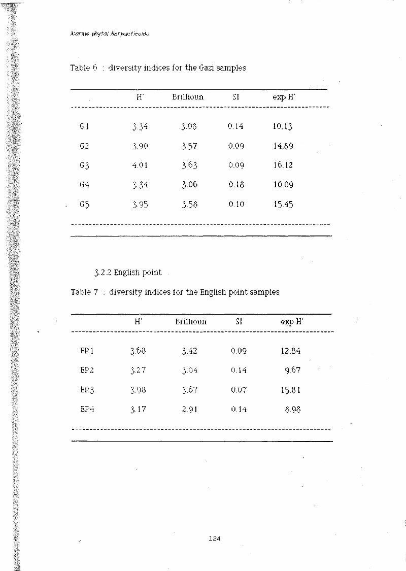
Marmç iryta'
Table 6 : diversity ind ices for the Gazi samples
H' Brillioun SI exp H'
G 1 G. 3 4 3.06 0.14 10.13
G2 3.90 357 0.09 14.69
G G 4 01 3-63 0.09 16.12
G 4 3.34 3-06 0.1Ô 10.09
G 5 3-95 3-5Ô 0.10 15.45
? T.J ia
Table 7 :
.2 English point
diversity indices for the English point samples
H' Brillioun SI ésp H'
EPI 'i c-. 0 .i. V1 O 3.42 0.09 12.54
EP2 'i “* *7. f. ¿j t 3.04 0.14 9.67
EP.3 395 3-67 0.07 15-61
EP4 .3.17 2.91 0.14 595
124

Man)if if/yta! da
Only by looking at the values of H’ for the different samples, one can see that these data, fluctuate w ithin the locality and that these fluctuations are comparable to inter-site fluctuation. I t is not very usefull to try to find out if differences between the two localities are significant or not. on this level. Although H‘ is widely used, it does not appear to be a good choise here.
Bearing in mind the above stated reasoning as well as tire richness data of Table 3 • it is obvious that H'. although widely used, is useless as a discriminator m this contest.
The fact that H' is not very usefull here can be due to the fact that the species lis t was not exhaustive, in other words, that the exact number of species occurring on Thalassodendron sp. is not known. Presence of all species is one of the assumptions made when calculating H'.
The calculation of H' is also dependent of for example, reproductive cycles and of "patchiness" (which can also be a consequense of the reproduction cycle of the species in question). This patchy occurrence is frequently encountered in the samples :
For example Picssccus cf. haœeJtoni is very abundant, in G3 (26 individuals out of IS 1) whereas it. is absent from G1 and only two individuals are found in G2. The same can be said of Dactylopusia tisboides {33 out of 1S2 in GS) and especially Esola hirsuta (61 out of 1S6 in G4). A number of other species exhibit minor "patchiness".
In tlie case of Esola h irsute , the reproductive cycle almost certainly plays an important role.
A clear cut case of how the reproduction cycle could influence the calculation of H' is the one of Eudactylopus fasciatus This species has been recorded in some cases and not in others. Samples from the same place, but taken w ith an interval of six months, showed a marked difference in abundance (no absolute values are known for the July '90 samples but thorough examination of quite large samples revealed very few animals in some while in others the species was not present at all (pers. obs.)).
I t can be expected that such is the case for lots of other species as well. The data obtained can be regarded as a reflection of these inherent problems.
The Brillioun index shows the same pattern as the H' values, confirming the findings of Heip et al. ( 19ÔÔ) that this index is not suited for meiobenthic assemblages. Though Pielou (1975) states that this index is better than H' for small populations.
For the Simpson index the same thing can be said.The exp H' is clearly the best discriminator thusfar (this has also been
demonstrated by Kempton (1979)). On the fam ily level a difference of 2 units is observed. Although this is not a very spectacular difference, i t does confirm the general trend found in the data of Table 3-
125

Marm ityta! Harpxt¡conia
For tlie average values of exp H' on species level of botli localities (summation of all species and their respective abundances for Gazi and English point) the following values were found :
exp H’ Gazi = 20.ôb
exp H 'English point = 14.95
On the species level the differences in exp H' for both localities are more clear cut than on the farnilv level.
3 .2.3 Margalef 's index
Comparison of the two sites as evalufced by Margalef’s index, an index based (unlike the indices mentioned above) on species richness alone :
Dm* = (S -l)/lnN
The following values were found for the separate samples
Table d : Margalefs index of diversity
Sample Dttlé
Gl 3.375G 2 4.143G 3 4.365G4 3.951G5 4.379EPI 3.157EP 2 .3.772EP 3 3.623EP 4 2.314
126

Marim ir.yfa'
vVhen one considers the total number of species and their abundance per site the following values are found :
t W dasi = b . 3 17
Dtu¿ English Point = 4.406
These values are also a good reflection of the (evident, see Table 3) difference in species richness. The values for G1 (3-375) and EP4 (2.314) can be regarded as exeptions to the general trend that the values for Gazi Bay are are always higher than those for English Point. This cannot be said of the H’ values for both sites.
So, concluding one can say that exp H' is toe best discriminator followed by species richness (as expressed by Margalef's index), H', Simpsons index and the Brilliou.n index are not suited. The fact that exp H' has toe best, discriminating abilities and not Dttlé as found by Kempton (1979) can be due to the relative important, dependence on sample size of the latter.
The differences in physical stress (which are inevitably present), together w ith toe (not proven) pollution stress may account for toe differences in species richness found between English point and Gazi Bay. Tudor Creek and tire tidal channel can hardly be called highly polluted sites (although there is no heavy industry since the harbour and associated industry are at the other side of Mombasa Island, there may be influence from the sewage of Mombasa and from the hospital and the meat factory discharges). Concluding that toe observed differences are entirely due to human induced stress factors is too rash. Monthly investigations of toe composition of the harpaeticoid community
f are necessary to evaluate this problem on a more solid basis.The differences in species richness on the other hand, are too large to be
neglected. One could argue that at least twelve species occur at English point that don't, occur at Gazi, but. the other way around, twenty eight species are confined to Gazi alone.
Already at the fam ily level, there is a difference of 4 units, and as Herman & Heip (19Ô6) point out, one really doesn't, have to perform the time consuming dissections (to arive at toe species level) to come to a conclusion in all cases. This is also illustrated by the diversity analysis performed on the fam ily data of Table 5 :
127

iVanm- irs/ta? Martxzütjcdióa
Table 9 : Family level diversity
Gazi English point
H' 333 3.04Brillioun index 3.O0 2.95Simpson index Ö. 13 0.14exp H’ 10.07 Ô.23
I t is clear that exp H‘ is the best discriminator.
Considering further the M/C ratios, which don't show a very convincing difference when applied to phytal assemblages, the use of the phytal harpaeticoid community and the measure of its diversity by means of the simple species richness data, must at least be kept in mind as a cheap and quite practical alternative for other methods.
But w ithout certainty about pollution (is there polution and if so of what kind and to what extend), and w ithout data on the (possible) effects on the macrofauna of this pollution (Rafiaëlli & Mason, 1961 ), this conclusion is a b it
1 premature. I t is then of course also the question if any differences in macrofaunal composition are not caused by other (e.g. physical) factors than pollution. The simplest conclusion, judging from tire above mentioned data, is that the phytal harpaeticoid "community" of Gazi bay is more diverse (in the literal meaning of the word i.e. having more species than ...) than the English point (Tudor) "community". About the reasons for this difference, be it pollution or intrinsic properties of the ecosystem, nothing firm can be concluded.

íVírr'rif í yta i .Va
6. Twinspan analysis.
TWIN SPAN (TWo-way INdicator Species ANaiysis) is a FORTRAN program in which species as well as samples are classified. The indicator analysis is not the real basis of the method so the name TWINSPAN can be confusing. A better name is "dichotomized ordination analysis". So the basic method used in this program is the division of ordinations.
This analysis is dealt w ith separately because in se it has nothing to see with the use of harpaeticoid diversity to separate the two locations.
The output (see addendum) contains all information in a very compact manner.
The dendrogram resulting from this analysis and showing graphically the separation of the different, samples (stations) looks like this :
G1G2
G4G5
G3 EP1EP2
EP3 EP4
The two locations are nicely separated although a few irregularities occur. There are a lo t of species w ith a high 'cut level' (weight for the abundance of a species) that are common to both localities. The species that caused this 'smooth' separation are present, in lower numbers when compared to those common species.
129

Thus, the grouping can be interpreted as being the result oí a specific assemblage of species occurring exclusively and w ith few representatives in one of the two localities.
Fsola longicauda, Bradyellopsis sp, Paralaophonte sp., Amphiascus cf. parvus and Diarthrodes sp. B are all species w ith a high cut level for English point and occur in very low numbers or not at all in Gazi Bay.
For Gazi Bay, Bsola hirsuta, Liosaccus ham iltoni, Eudactylopus andrewi t Porcellidium clavigerum and M etis ignea are the dominant species. Of those, only Porcellidium clavigerum is found (at very low numbers) at. English point.
The separation of G 3 from G1 and G 2 (all tírese samples come from the artificial channel) can be due to tire abundance of Diosaccus ham iltoni (cut level 5 in G 3, 2 in G2 and 0 in Gl). Bobertaonia propinqua , Tisbintra nankaurica and Scuttelidium sp. B are species that are present in G 3 only (cut level 2). This toghether w ith the lach of Motis ignea in G3 and its abundance in G 2 and Gl could be an explanation for the fact that. G 3 is separated from the samples G4 and G5 from the main channel.
The separation of EP1 and EP2 from the two other samples is a consequence of, like demonstrated above, the inequal species distribution. In this case mostly Amphiascus cl. parvus , Bradyellopsis sp and Paralaophonte sp are responsible.
This TWINSPAN analysis confirms tire separation of Gazi Bay and English point, harpaeticoid assemblages as evaluated by means of diversity analysis. A ll this can thus be seen as a 'confirmation1 or a justification of the previously used methods to detect differences in the two species assemblages considered.
Bearing all the above mentioned statements in mind, one could say that, in this context of evaluating tire use of Harpacticoida in pollution monitoring through diversity- and TWINSPAN analysis, it can be sufficient to focus on one particular taxonomic group instead of considering tire complete meiobentlricspectrum.
A li figures, species lists and TWINSPAN printout are to be found in tire addendum.
130

References
- Help i960. Meiobenthos as a tool in the assessment of marine environmental quality. In A.D. McIntyre and J.B. Pearce (eds.), Rapport et Frocés-verbaux des Reunions Conseils International pour l'exploration de laMer 179 : 152-107
- Herman P.M.J and C. Heip, 19ÔÔ. On the Use of Meiofauna in Ecological Monitoring : Who Needs Taxonomy? M ar PoJJvtion Bull, 19 , n° 12 : 665-660.
- Hemrninga M .A. and F.J. Slim. Nutrient fluxes between mangroves, seagrass meadows and coral reefs as viewed from a seagrass perspective.JJydrohioJogia (in press).
- Hicks G.R.F., 1977. Species composition and zoogeography of marine phytal harpaeticoid copepoda from Cook Strait, and their contribution to total phytal meiofauna. N I. Journ Mar. andFroshw. Res., 1 1 (.3) : 441-69.
- Lang K., 1946. Monographie dor Harpacijcidon. Hakan Ohlosson, Lund, 2 vol. : 1-1662.
- Pielou E.C., 197b. Ecological Biversity. Wiley, New York.
- Raffaelli D.G. and C.F. Mason, 1961. Pollution monitoring with meiofauna using the ratio of nematodes to copepods. Mar. Pollution Bull, 12(b) : 15Ô-63- * -
- Wells J.B.J., 1979. Roy fo in Ule identification o f marino harpaeticoid copepoda. Amendment bulletin N. 2. Zool. Publ. Victoria Univ.Wellington. 7.1 *
131
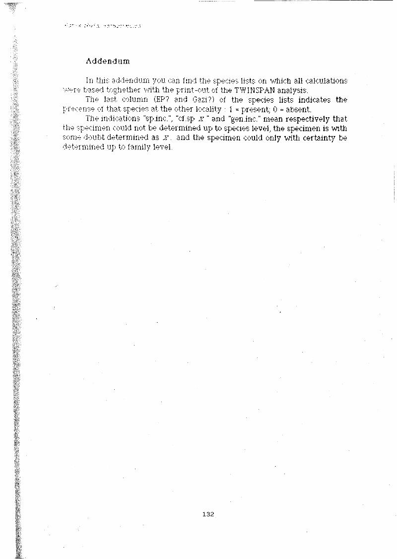
’ ’ .'I.- '? T v. v . . t* - . ’
A d d e n d u m
In this addendum you can iind the species lists on which all calculations were based toghether w ith the print-out oí the TWINSPAN analysis.
The last column (EP? and Gazi?) oí the species lists indicates the precense oí that species at the other locality : 1 = present; 0 = absent.
The indications "sp.inc.". “cf.sp w " and "gen.inc." mean respectively that the specimen could not be determined up to species level, the specimen is w ith some doubt determined as x . and the specimen could only w ith certainty be determined up to family level.
132
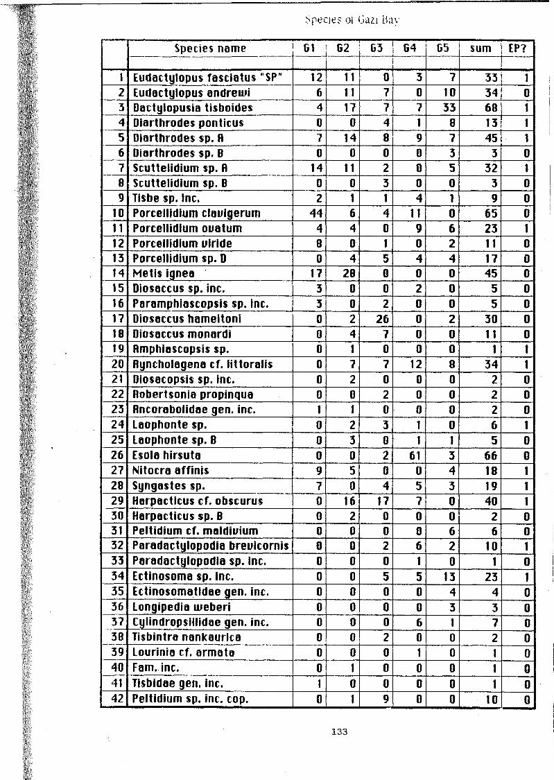
Specie? oí Gazi Bay
Species name Gl G2 G3 G4 G5 sum EP?
1 Eudactylopus fasciatus "SP" 12 11 0 3 7 33 12 Eudactylopus andrewi 6 11 7 0 10 34 03 Dactylopusia tisboides 4 17 7 7 33 68 14 Diarthrodes ponticus 0 0 4 1 8 13 15 Diarthrodes sp. B 7 14 8 9 7 45 16 Diarthrodes sp. B 0 0 0 0 3 3 07 Scuttelidium sp. fl 14 11 2 0 5 32 18 Scuttelidium sp. B 0 0 3 0 0 3 09 Tisbe sp. inc. 2 1 1 4 1 9 0
10 Porcellidium claulgerum 44 6 4 11 0 65 011 Porcellidium ouatum 4 4 0 9 6 23 112 Porcellidium uiride 8 0 1 0 2 11 013 Porcellidium sp. D 0 4 5 4 4 17 014 Metis ignea 17 28 0 0 0 45 015 Diosaccus sp. inc. 3 0 0 2 0 5 016 Paramphiascopsis sp. inc. 3 0 2 0 0 5 017 Diosaccus hameltoni 0 2 26 0 2 30 018 Diosaccus monardi 0 4 7 0 0 11 019 Amphiascopsis sp. 0 1 0 0 0 1 120 Ryncholagena cf. littoralis 0 7 7 12 8 34 121 Diosacopsis sp. inc. 0 2 0 0 0 2 022 Robertsonia propinqua 0 0 2 0 0 2 023 Rncoraboiidae gen. inc. 1 1 0 0 0 2 024 Laophonte sp. 0 2 3 1 0 6 125 Laophonte sp. B 0 3 0 1 1 5 026 Esola hirsuta 0 0 2 61 3 66 027 Nitocra affinis 9 5 0 0 4 18 128 Syngastes sp. 7 0 4 5 3 19 129 Harpacticus cf. obscurus 0 16 17 7 0 40 130 Harpacticus sp. B 0 2 0 0 0 2 031 Peltidium cf. maldiuium 0 0 0 0 6 6 032 Paradactylopodia brevicornis 0 0 2 6 2 10 133 Paradactylopodia sp. inc. 0 0 0 1 0 1 034 Ectinosoma sp. inc. 0 0 5 5 13 23 135 Ectinosomatidae gen. inc. 0 0 0 0 4 4 036 Longipedia weberi 0 0 0 0 3 3 037 Cylindropsillidae gen. inc. 0 0 0 6 1 7 038 Tisbintra nankaurica 0 0 2 0 0 2 039 Lourinia cf. armata 0 0 0 1 0 1 040 Fam. inc. 0 1 0 0 0 1 041 Tisbidae gen. inc. 1 0 0 0 0 1 042 Peltidium sp. inc. cop. 0 1 9 0 0 10 0
133

Species ot English point
Species name EP1 EP2 EP3 EP4 sum Gazi?»
1 Dactylopusia tisboides 21 40 14 7 82 12 Diarthrodes sp. ñ 13 1 0 0 14 13 Diarthrodes sp. B 0 ? 11 0 18 14 Diarthrodes ponticus 16 13 14 3 46 15 Paradactylopodia breuicornis 6 19 4 2 31 16 Eudactylopus fasciatus "S" 0 1 2 0 3 1? Eudactylopus fasciatus "SP" 0 0 3 4 7 18 Rmbunguipes rufocincta 1 0 0 0 1 09 Rmbungulpes similis 0 1 0 0 1 0
10 Teissierella sp. inc. 3 6 2 8 19 011 Amphiascopsis sp. 9 3 0 0 12 112 Ryncholagena cf. littoralis 23 27 22 32 104 113 Amphiascus cf. paruus 0 0 12 0 12 014 Paraidya sp. inc. 0 2 9 0 11 015 Scuttelidium sp. R 4 2 8 4 18 116 Laophonte sp. 13 12 6 7 38 117 Heterolaophonte strdmi 2 0 0 0 2 018 Paralaophonte sp. inc. 7 12 0 0 19 019 Esola longicauda 0 3 11 5 19 020 Esola sp. inc. 0 0 3 0 3 021 Laophontidae gen. inc. 0 0 2 0 2 022 Porcellidium clauigerum 0 0 1 0 1 123 Porcellidium ouatum 1 0 3 0 4 124 Syngastes sp. 1 0 0 0 1 125 Harpacticella sp. inc. 1 0 0 0 1 026 Harpacticus cf. obscurus 15 6 9 12 42 127 Nitocra affinis 7 0 9 16 32 128 Ectinosoma sp. inc. 16 0 9 0 25 129 Bradyellopsis sp. inc. 0 0 0 12 12 0
134

F\Y INSPAN print out
568971234
18 Para s inc - - 1 ------- 00000031 Pelt ma Id --------3 -------------- 00000034 Ecte ginc --------2------ 00000035 Long webe --------2------ 00000036 Cyl i ginc — 31------ 00000038 Lour arma — 1------- 00000026 Eso 1 hirs — 522---- 00000113 Pore sped - 2223---- 0000108 Scut speb -----------2----- 000011
16 Dios hame -2-25---- 000011Robe prop -----------2----- 000011
37 Ti sb nank ---- 2----- 00001128 Syng spec 3-3221--- 0001017 Dios mona -2 — 3---- 0001141 Pelt s ico - 1 — 3---- 000119 Ti sb si nc 21211---- 001000
15 Dios s i nc 2-2------- 00100125 Laop speb -21 1 ------ 0010012 Euda andr 34-43---- 001010
10 Pore c lav 534-2— 1- 00101012 Pore vi ri 3 — 21---- 00101014 Met i i gne 45-------- 00101121 Dioc s i nc -2-------- 00101123 Anco ginc 11-------- 00101130 Harp speb - 2 -------- 00101139 Fami ince -i-------- 00101140 Ti sb ginc 1---------- 0010115 Diar spea 3433341— 0011
1 1 Pore ovat 2233-1-2- 00111 Euda fase 4423— 132 0107 Scut spea 4423-2232 010
33 Ect i spec — 3434-3- 0113 Dact t i sb 243535543 1000
27 Ni to af f i 33-2-3-34 100129 Harp obsc -43-44334 100120 Rync lito -34335555 10132 Para brev — 3223422 1014 Diar pont — 1324442 110
24 Laop spec -21-24433 11052 Brad s inc ----------4 1110044 Teis s inc ------2323 1110149 Eso 1 long ------- 243 1110119 Amph spec -1--- 32 — 11110042 Ambu simi ------ 1 — 11110043 Ambu rufo ----- 1---- 11110047 Hete stro ------2---- 11110048 Parí s inc ------34 — 11110051 Hart sinc ----- 1---- 11110045 Amph parv -------- 4- lilloi46 Pard sinc ------- 23- lilloi50 Laop ginc ----- - 2 - lilloi53 Eso 1 sinc -------- 2- l i l l o i6 Diar speb --- 2 — 34- 11111
000001111001110001
001001
135

Visit to K.M.F.R.I., Mombasa
Name: J.F. TackAddress: Free University of Brussels
Laboratory of Ecology and Systematics'Pleinlaan 2 B-1050 Brussels 5 Belgium
Period: 10th March 1991 - 1st April 1991Aims: A. Preliminary research "Comparative physiological ecology of
the oyster Crassostrea cucullata "B. Commercial Oyster Culture - Kenya: Financial Analysis
A. Preliminary research "Comparative physiological ecology of the oyster Crassostrea cucullata "
The oyster Crassostrea cucullata is a suspension feeder. Three methods have been commonly used to study particle filtration by bivalves.
The first method involves channeling water into and from shell cavities with devices which collect all water flowing through the gills. This method has been criticized because oysters may not behave normally when subjected to the stress of the collecting device.
The second method involves measurements of rates at which undisturbed bivalves clear particles in standing water. Objections to studies in standing water are that previously filtered material may be resuspended and refiltered (recycled) and also that particle concentrations will change with time.
The third method makes use of chambers of flowing water. This method makes it possible to measure differences in numbers of particles, amounts of Particulate Organic Carbon (P.O.C.), and amounts of chlorophyll
136

entering and leaving the system. Differences are attributed to filtration by the animals. Water flowed continuously over the oysters under conditions approaching those of the natural environment. This also served to avoid recycling.
In the study "Comparative physiological ecology of the oyster Crassostrea cucullata " we will make use of the third method. The main purpose during our visit to Mombasa was testing this method making use of the chambers we were using in a similar study ""Comparative physiological ecology of the oysters Crassostrea gigas and Ostrea edulis "
The experiments were conducted at the K.M.F.R.I. (Kenya Marine and Fisheries Research Institute) - Mombasa, Kenya. Water for all studies was pumped from a source 0,5 m above the bottom, in the Tudor Creek, to a constantly overflowing overhead trough in the laboratory. Water flow was ± 1 l/min (in each chamber).
Several difficulties arose during the experiments:- The small amounts of P.O.C. and chlorophyll in the water
made it very difficult to measure the differences between the inflow and the outflow of P.O.C. and chlorophyll.
- The silicone used became mouldy after a period of six days.
At the moment we are building new chambers. The new chambers will allow us to measure P.O.C., chlorophyll, and other variables more exactly. These chambers will be finished in the early part of the year 1992.
B. Commercial Oyster Culture - Kenya: Financial Analysis
You can find the results of this study in the annex
137
/ 4 6 9 2
COMMERCIAL OYSTER CULTURE - KENYA:
FINANCIAL ANALYSIS
J.F. Tack, M. Sc.Free University of BrusselsLaboratory of Ecology &SystematicsPleinlaan 2B-1050 Brussels 5Belgium
138

Summary and conclusion
Collecting big oysters of the species Crassostrea cucullata at the current rate will lead to the overexploitation of this species in Kenya. Moreover, the method which local gatherers use to collect the oysters results in damage to the mangrove trees.A commercial oyster culture would solve both problems and financially it seems to be an interesting investment.There would be an internal rate of return of 22,8% on a yearly basis. The Benefit-Cost ratio is 1,69. This means that costs can rise by 69%. The Net Present Worth is 51,750,000 KES after 25 years (investment: 10,041,000 KES).
139

A. Introduction
Six years ago the Kenyan Government requested the Belgian Government’s collaboration in the field of Marine Sciences. The Free University of Brussels and the Laboratory of Ecology and Systematics under the direction of Prof. Dr. P. Polk in particular, accepted the challenge. After 6 years it has become obvious that this collaboration has borne fruit and continues to generate useful results.
In the past several projects like the Kenyan Belgian Project in Marine Sciences failed because the linkage between research, education and equipment was lacking. What can a specialist do without facilities? What use is equipment without expertise and teaching? The importance of the simultaneous development of these three components cannot be overestimated. The teaming-up of Kenyan and Belgian experts was a guarantee for the scientific value of the work.
Originally the project was a collaboration between the K.M.F.R.I. (Kenyan Marine and Fisheries Research Institute) and the Free University of Brussels. In the meanwhile, experts of the universities of Ghent, Antwerp, Limburg, Leuven and Liège became involved. The Institute for Marine Sciences (IZWO) is collaborating for Scientific Literature Search. Kenyan
' Scientists got specialized training in different universities and institutes in Belgium. Belgian experts and students carried out research in Kenya. The exchange of information, know-how and experience proved to be very successful.
The EEC Research Project "Dynamics and Assessment of Kenyan Mangrove Ecosystems" has integrated the famous Delta Institute (The Netherlands), the University of Nijmegen (The Netherlands), Kenyatta University (Kenya) and Nairobi University (Kenya) into the existing group.
The Kenyan Belgian Cooperation in Marine Sciences, which started as an agreement between the Kenyan and Belgian Governments, continued to extend its contacts. Donors now include the Belgian National Science Foundation, the Flemish Interuniversity Council, the European Economic Community, IOC-UNESCO and UNEP.
140

The documentation centre of the project has in the meantime developed into an independent offshoot of the project, known as the IOC- UNESCO-RECOSCIX project (director: P. Pissiersens).
While fundamental research is developing at an accelerated speed, applied research can give practical results immediately and throughout the next decade.
In 1986, the director of the Kenyan Belgian Cooperation in Marine Sciences was asked by the Minister for Development Cooperation to initiate scientific activities which might result in profit; up to then the activities had been purely scientific.
Kenyan officials view commercial oyster culture favourably because the Kenyans are obviously keen to participate in ventures which generate funds and create employment.
A commercial oyster culture would also conserve the mangrove ecosystem in the short term and benefit the whole of the marine ecosystem in the long term.
B. Kenya Today
Government and Economy
President Daniel arap Moi holds executive power assisted by a Vice President and Cabinet chosen from the legislature, the National Assembly. This body consists of 158 members elected by universal suffrage, 12 Presidential nominees, the Speaker and the Attorney-General. The Assembly's term is for five years unless it is dissolved by the President or its own majority "no confidence" vote.
141

The process of government in Kenya is essentially democratic, but there is only one political party, the Kenya African National Union (KANU).
Kenya is an independent republic, a member of the Organisation of African Unity (OAU), the Commonwealth and the United Nations.
The country's record of stability and sound government, as well as its development performance since Independence in 1963, have placed it among the most prosperous nations in Black Africa. It is a major recipient in Africa of international development aid.
On its own account, Kenya is among the world's leading exporters of quality coffee, teas, and pineapples. Other primary exports are horticultural produce, pyrethrum, sisal and other cash crops. Tourism is an important source of foreign revenue, with further substantial income resulting from Kenya’s position as the regional center for communication, insurance and general commerce.
Geography
Kenya is an independent republic with an area of 582,644 sq km, including approximately 13,600 sq km of inland water. It is bounded in the north by the deserts of Somalia, Ethiopia and the Sudan; to the east by Somalia and the Indian Ocean; and to the south and west by Tanzania and Uganda.
The country is roughly bisected by the equator, extending as it dies between latitudes five degrees north and 4.40 degrees south. Mean longitude is 40 degrees east, which is three hours ahead of GMT.
Broadly, the country may be divided into four main physiographic regions:
142

- The Rift Valley and Central Highlands:Fertile, mountainous, lake-studded, and the most developed region economically and in terms of human settlement.
- Western Kenya:Low plateau farmland east of Lake Victoria.
- Northern and Eastern Kenya:A vast T-shaped expanse of country from west of Lake Turkana (Rudolf) across the north to the Somalia border and to the Tanzania border in the south. This is mainly semi-arid rangeland for nomadic pastoralists and wildlife.
- The Coastal Belt:480 km of Indian Ocean littoral, including coral reefs, beaches, mangroves, and a narrow fertile strip where sub-tropical agriculture is practiced and which gives way to bush and semi-desert.
Climate
With an altitude that ranges from sea level to 5,200 m, the temperature, rainfall, and humidity variations are extreme.
In relation to the four physiographic zones, the climate and land-types can be characterized as follows:
- The Rift Valley and Central Highlands:This highland region of Kenya generally experiences invigorating, fairly cool conditions, rather like a Swiss summer. The climate ranges from temperate in the Central Rift Valley to arctic on the Mount Kenya peaks.
143

The land here is the most productive in Kenya. In the uplands, between 1,500 - 2,000 m, the greater part of Kenya’s agricultural output is produced. In the Rift itself, production is mixed * crops, dairy and livestock.The central massif of Mt. Kenya and the high Aberdares form the country’s main water catchment area, with rainfall of up to 3,000 mm per year on the mountains, producing run-offs to the main Rift lakes.
- Western Kenya:Hot, moist, with the rains spread fairly evenly through the year. Most of the rain falls in the early evening.
- Northern and Eastern KenyaThe land ranges from lava desert around Lake Turkana (Rudolf), where west of the lake rainfall averages below 225 mm per year and temperatures rise to 39°C; through sand desert at the Chalbi in the north, arid bush supporting pastoral activities, vast dry grass and acacia rangeland, down to the soda lake of Magadi in the south, where again temperatures can be as high as 38°C.
- The Coastal Belt:The coral beaches are hot with about 70° humidity but tempered by breezes. Then comes a narrow coastal plain, suitable for agriculture (fruits, nuts, cotton, dairy) but this soon gives way to thorn scrub and semi-desert.
C. Location of the oyster culture
Geography
480 km of Indian Ocean littoral, including coral reefs, beaches and mangroves, and a narrow fertile strip where sub-tropical agriculture is practiced.
144

Kenya possesses 22 extensive mangrove creeks, with a total surface area of 52,000 hectares.
C lim ate
The coral beaches are hot with about 70° humidity but tempered by breezes. Then comes a narrow coastal plain, suitable for agriculture (fruits, nuts, cotton, dairy) but this soon gives way to thorn scrub and semi-desert.
The climate of Mombasa can be considered to be representative:- Altitude: 17 m- Rainfall: Average minimum 20 mm (February) to maximum
240 mm (May) average annual 1,000 -1 ,250 mm- Sunshine: Averaging a maximum of nine hours per day in
March and a minimum of seven hours in May- Temperature: Mean annual minimum: 22° C
Mean annual maximum: 30° C.
Location
The oyster culture will be spread out along the whole length of the Kenyan coast (in different mangrove creeks). Thus we are able to minimize the risks (oil pollution, bacterial pollution, etc...) and the distances between oyster culture and consumer.
145

D. Oyster Culture
The mangrove oyster Crassostrea cucullata
The scientific name of the oyster is Crassostrea cucullata. This species is extremely abundant in the mangrove creeks present in the Kenyan coastal area, where it grows on the extensive air-roots of the mangrove trees. They live so closely together, however, competing for space and food, that the majority never reach the size necessary for human consumption. In fact, most of these oysters are only 2 to 4 centimeters in size.
As far as taste and appearance are concerned, the Kenyan oyster compares favourably with its European counterpart; a rich creamy yellow color and a stronger flavour are characteristic features.
Present situation
About 40,000 oysters are , presently, being cultured in Gazi, 48 kilometers away from Mombasa.
Gazi is linked to Mombasa by an asphalt road in good condition. There is a river to be crossed by pontoon, however, making it a trip of approximatively one hour by motor vehicle.
The village of Gazi lies next to the road and about two km from the mangrove creek where the experimental oyster plot is located. The path leading to the site necessitates a four-wheel drive vehicle.
The villagers and the village headman are very enthusiastic about the culture; they were hired and paid to collect the wild oysters, erect, clean and maintain the racks, etc... As a consequence, they look after the site to protect their interest in it.
146

Local and international Market
The local market:
Kenya has a well developed tourist industry; a number of high-class restaurants are found in and around the touristic cities (Nairobi, Mombasa).Several restaurants in Mombasa and Nairobi presently serve fresh oysters on ice. While still smaller than the European variety, these oysters reach the size that can be attained after two to three years of culturing.At present, the restaurants buy the oysters from local gatherers who search extensive areas to find such big specimens. The method which local gatherers use to collect the oysters results in damage to the mangrove trees.Collecting big oysters in the wild is leading to the virtually complete removal of these specimens. This is followed by a substantial increase in price, since more extensive areas will have to be searched. In these conditions, moreover, the restaurants cannot be guaranteed freshness. At the moment restaurant owners pay 1 to 2 KES for each oyster, but this includes a majority of smaller specimens. Moreover, some refuse is always présent. Tamarind restaurant (one of the biggest restaurants in Mombasa) is willing to pay 6 KES/oyster (400,000/year ; starting in 1995).The sale of cultured oysters to Kenyan restaurants will generate local and foreign currency.
The International Market:
Kenyan oysters can be exported to generate foreign currency:- the price of the Kenyan cultured oysters is far below that of
the European ones.- there exists an excellent transportation network linking
Mombasa to the rest of the world.It is difficult to predict at this stage which countries would be the best targets for export. Many restaurants in Europe are interested to serve Kenyan oysters as a speciality. The sizeable expatriate
147

communities in other African countries and in the Middle East could also be targeted.
Land Use
90% of the tidal area of the mangroves is property of the Kenyan Government. It would be possible to rent this area for a period of 99 years. Because the project will generate foreign currency while at the same time protecting the mangrove ecosystem, the rent would be a nominal amount.
Social aspects
The implantation of the oyster culture does not affect other activities of the local population.
As far as possible, personnel will be hired and material bought in the villages in the immediate proximity of the oyster culture. As a consequence, the local population will look after the site to protect their interest in it.
Development of the oyster culture
Prior to initiating business operations in Kenya, we need to obtain a number of approvals and registrations, some general and others applying to specific activities only. To expedite the processing of these applications, we will make use of the services of the Investment Facilitation Committee at the Investment Promotion Centre (IPC). The Centre assists investors by helping them to complete an "Investment Proposal Form" that contains nearly all the information required, thus transforming the investment application procedures into a "one-step" process.
148

We will entrust the development of the oyster culture to a specialized firm for a period of three years. This firm will also be responsible for the education of the local personnel and of a future local manager, the delivery of the necessary know-how and the creation of a national and international distribution network. The advantage of involving a specialized firm is the low cost compared with the wages of several expatriate experts. This firm is called "the expert" in the financial analysis below.
Export Processing Zone incentives (Kenya)
- duty and VAT exemption on imported machinery, equipment, tools, spare parts and raw materials
- 10 years tax holiday and thereafter a flat tax rate of 25% on profits for the next 10 years
- no withholding tax on dividends- exemption from exchange control- operations in foreign currencies permitted- 100% foreign ownership permitted- exemption from VAT on locally procured goods- one single licence for all manufacturing activities- competitive lease/rental fee- available infrastructure and utilities at cost
Number of oysters
Two hundred racks will be built every year. Those racks can carry720,000 oysters.
149
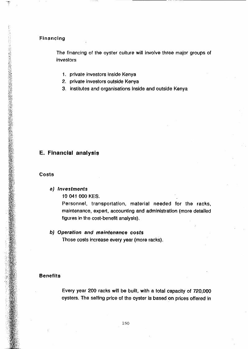
Financing
The financing of the oyster culture will involve three major groups of investors
1. private investors inside Kenya2. private investors outside Kenya3. institutes and organisations inside and outside Kenya
E. Financial analysis
Costs
a) Investments10 041 000 KES.Personnel, transportation, material needed for the racks, maintenance, expert, accounting and administration (more detailed figures in the cost-benefit analysis).
b) Operation and maintenance costsThose costs increase every year (more racks).
Benefits
Every year 200 racks will be built, with a total capacity of 720,000 oysters. The selling price of the oyster is based on prices offered in
150

1991 for oyslers delivered in 1995 (more detailed figures in the cost-benefit analysis).
Cost-benefit analysis
Definitions:
Present worth:
If someone is earning 1,000 $/year for a period of five years, the last1,000 $ has not the same value as the first 1,000 $.The process of finding the present worth of a future value is called "discounting". The interest rate assumed for discounting is the "discount rate". The interest rate used for compounding assumes a viewpoint from here to the future, whereas discounting looks backward from the future to the present.Generally the discount rate is a number between 8% and 12%. We will base our cost-benefit analysis on a figure of 12% (a worst-case assumption).
Benefit-Cost Ratio
This is the ratio obtained when the present worth of the benefit stream is divided by the present worth of the cost stream.If the benefit-cost ratio is less than 1, then the present worth of the costs at this discount rate exceeds the present worth of the benefits, and we will not recover our initial expenditure plus the return on our investment from the project.Note that the absolute value of the benefit-cost ratio will vary depending on the interest rate chosen. The higher the interest rate, the lower the resultant benefit-cost ratio, and, if a high enough rate is chosen, the benefit-cost ratio will end up below 1.One convenient aspect of the benefit-cost ratio is that it can be used directly to find out by how much costs could rise without making the
151

project economically unattractive. E.g., a Benefit-Cost Ratio = 1.69 means that costs can rise by 69% before the benefit-cost ratio would reach the critical value of 1.In practice, it is common to compare the present worth of the net benefit with the present worth of the investment cost plus the operation and maintenance costs.
Net Present Worth:
The most straightforward discounted cash flow measure of project worth is the net present worth (often abbreviated as NPW). This is simply the present worth of the incremental net benefit or incremental cash flow stream. The net present worth may also be computed by finding the difference between the present worth of the benefit stream less the present worth of the cost stream.A project is financially interesting when the NPW is positive.
Internal Rate of Return:
This is the discount rate that makes the net present worth of the incremental net benefit stream or incremental cash .flow equal zero. This discount rate is called the internal rate of return. It is the maximum interest that a project could pay for the resources used if the project is to recover its investment and operating costs and still break even. It is the "rate of return on capital outstanding per period while it is invested in the project".The internal rate of return is a very useful measure of project worth. It is the measure the World Bank uses for practically all its economic and financial analyses of projects and the measure used by most other international financing agencies.
152

Cost-Benefit Analysis (x 1,000 KES)
Remark: During the period of investment we increased the costs with10% on a yearly basis. During the period with a positive cash flow we did not increase the costs. Here the increase of the costs would be followed by an increase of the benefits.
153

Cos
t-Ben
efit
anal
ysis
(x
1,000
K
ES)
toCLXUi
O O O O O O O O O O O O Q O O O O O O O O ' o t o o o o o o o o o o o o o o o o o o o o ^ Of * t<0<0(0(0<0(0<0<0(0(0(0(0(0(0(0(0<0(0(0<C\l r r
oatocra
O O O t - T ~ T ~ T — T— t— T - T — T - T — T - t — T * T — r — r - r ” T ~ T - T - ’ ^ - T ~ *O O t-CNJCMC\ÍC\1C\ICSJC\JC\JOJC\JCNJC\I(MCNÍCNJC\IC\IC\JCMC\JC\JC\IT j- V - >r— t — r - T— T“ * T— T“ T” ▼— T- T— r— ^ T— T"~ T“ T “ V “ T “ T“ T “ T“
tooraDC
tT O C O O O O O O O O O O O O O O O O O O O O O O OCM^tNrrrrrrrrrr-rrrrrrT-rrrrr
ras
3o.Ora
o o o o o o o o o o o o o o o o o o o o o o o o oCON^T-COlOCMaXOnOSTTr-OÖinWOXOraON^r-flOCMr-CVir5COrJ-|JOlO<0N.C0OOO>OOT-CSJCNJO,» tm iO (0 f^ r^
to
ra
toccotow .toa.
OCDOOOOjTiCÛCOOCMrKOf lÛOW^tDOOOCM^COOOOCJ■r-r-t->T--*f-C\JCMCMCVjCMrOCOCOCOCOTj-Tt-TtTfTfL0lOLO
^ w O O O O O O O O O O O O O O O O O O O O O O O O O° h O O O O O O O O O O O O O O O O O O O O O Ototo w*2 >* E O3
_ _ _ > o o o o o o o o o o o o o o o o o o o O O O O O O O O O O O O O O O O O O O O O O O O O O O O O O O O O O O O O O O O O O O O CMCM^t-«t(0(0OCOOOC\JOJ^^t(0(0OOOOOOCNJC\J NSTr<tT-r-COOO(D(OnOOONS^^WCMO>0> *r~T-O4CMCVJCMCOCOrfrtLOLOlOinC0(0h*<r N.h-
ra♦<o
Jr « SJ jd Xi u¡81°wo
o o o o o o o o o o o o o o o o o o o o o o o o oo o o o o o o o o o o o o o o o o o o o o o o o oTfID(OONTt(£)COOCMTf(OeOOCM'i(OeOOWit(DOOO(MT-T-i-T-T-fMwtMoiNonnnnTtTt'^^Tt-inin
na>>-
T-cviO'it t o i c s c o m o Mf)^io(DS®0)OT-wn^in 1 — r-t-T-T-T-T-T-CMCMCMCVJCMCvl
(1)
2500
KS
h/mon
th
gros
s

Cos
t-Ben
efit
anal
ysis
(x
1,000
K
ES)
~ inSZ 9) 0> XC w « * ' S3 .** $ ® O
i-oNo>BT-N(<)0)ino>in(on^OT-wo)(oœco^T-N innu)T-®0)©(CoooeootDOfflONO)Nois»MS S2E't|« ,i{'iot-w<ttoios(ooosa>so(Or-o>wo wnOr-^mmoioinoonioisoiffiwNitnooiooNW • - ■ CM CM CM CM CM CM CO CO
mT—COCOCOCO
szm«9a
*o
Uic?o
•COSOïtO LO CO lí) r- O) CO O r- co CO CO CO CO Z.,-.COo>u> N-coCDIOT“ r COo> in T — h-COO LOCDCOCO T “* O CO IOIOCMCMC7>o> to M"COT“COr*cm o T—COo>h- CO M in CO M-CMCOT~o>O)coCOh-COo o 0000CMCMCDCDo OJ—T- T-* CMCMCMCMCMCMCOCOCOCOTf Tf
toCOoo>■«t
Ui
a>ca>sz
o o o o o o o o o o o o o o o o o o o o o o o o oWW't^tOtOCOCOOOCMCM^TiiOCOWCOOOCMC^COCOCDlD0>OiCMCMCOCOO>O>CMCMininCOOOCMCMininTí cococ\íc\jf r T-T~inmooTí-Ttoocococor**KT-i-i-r-CMCNjCMOjCOCOCOCOCOCO t' tTj-Tf
CMoC'en
COo
Ui++Uioo
COo
^OSi-in0)<0NrU)0>C0Nr-U)0)nSi-tn0)C0Sr*in h- U)COinO(M^NO>CMii(C)0)t-^iDOOT-CO(OCOOP)U)COO oCO Oi -N O î î -O lO C O O C M ' tN O > r -C O tO C O O C V J U )SO )T -^onocMCMOncoco^ttTi-^^wioiniotototoiDcosN LOS)
o*«55COOOCDCOGOCOCOOOCOCOCOOOCOCDCOCOCOCOOOCOCOaOCDCOCOO C C C M Ô Ô O Ô O Ô Ô O C n O O O O O O O O Ô O O O O( O C D N N N N N N N N N N N S N N N N N N N S N N N
.2cËT3«XJic'55coooo<
UiocCOccu4-E‘co
OOOOCVKOO^OOCVtOO^COWCOO^tOOCNJCOO^COCMCO©COT-C^CMf^coCO^OittOWT-tOT-NCMCOOCO^frOo^<ONO>ocMnin«5ooot-o^(ONO>ocsinioíOT-f-T-t-T-T-CsJCMCMCMCMCMCMCOCOCOOCO
COa>
>-
■CMco-M-intoh-coo>o OJCO^U)(ONCOO)Oi-WO^U) •t-t- t-t— t- t- t- t-CMCMCMCMCMCM<t -oH
From
the
tenth
ye
ar,
taxe
s ha
ve
to be
paid

Cos
t-Ben
efit
anal
ysis
(x
1,000
KE
S)
m
ow
r-<iM))OnOWO)T-NSC\IO®OtDN^T-®T-U50)nTíT~Tf(Ma)cooooocncDoo->-ojTfcr5rft co'tT-ocj'tCMa>3t2*;SHc>f'.r'.of CMCMc»in©’«*oweoo>(£>r^,í,íT-T-coCOCMCM,- CM CM CO CO CM CO CO CO CO CO CM CM CM CM CM CM CM CM r-oIOr-r*in
0>ca>x>0>z
t - T f N O ) o c o o c o o ) i - ^ ( ö c o o c o o u ) c o i n o ) o « ) T “ C g i o co ín l ! T ^ C M 0 ) C 0 0 0 C 0 0 > t 0 n 0 ) < 0 O 0 ) U ) 0 > C 0 O 0 0 T - W C 0 < 0 ( 0 to¿2 : g ; M ; C M o h * . h - c o r ^ c M C M N . c o c D c o K O i n r >> * c o c o o o < r > < o c o _T5 CO OsJ C\J T - CM CM CO CO t }- CO CO r f CO CO CO CO CO CO CO CM CM CM I j
• « •5O
O
V)
OOOf^OOLOtOCO^OT-COCOCOOLOCMCOCOtOintOtOCO^^■COOCOMOlOin^r^W-rOO^rCOQíOON^COOïCVKOUÏ^lOOîCONCDt^OOOlOr-i-OOCMCM'M-COm'O-in inM-LOM-'M-’M-'t’M-'M'COCOCOCOCMCM0>COCMO)
4>Ca>CO
IDinrH
T3a>c3Oo«
T-Ttr^N-COCO'M-CO0>CMin<tOOslinCOO>CQCOCOlOCO^tCOC0Tfr^r-inO)CvlU)NO(NJU)OOi-^NT-lOOlOOin^NC3M M - C M N i O l O l O T f C O C O C N J r - O O O C O a D N S C D t O t n i O M - M -CÓCMCMt-r'f-,T-r-r’T“ T-T-r*i"
rinoCO
V)oo
CM
©4«rac3ooV)
C0h'CMt0f l CM'<tT-CMr h-CniiJC0C0C0O«0’tC0C0' C0050)CDr-n(COLnO(OtMOOIflCMOOOtD^Oi-OOlOON(Oint O N N f f l l f l l O ' i ^ O n W N W W r - r - r - T - r - T - O q O O Od d d d d d d d d d d d d d d d d d d d d d d o d
raV>•T*CMCO'^in<Oh'eOO>OT-CMCO'tlOCDh-COO)0-i-CMiO'<tlO
t- t- t- t- t- it- t- t- t- t-»CMCMCMCMCMCM OI-

Results Cost-Benefit analysis:
Net Present Worth (NPW): 51 750 000 KES Internal Rate of Return: 22,8%Benefit-Cost Ratio: 1,69
157

Cash
-flow
(x
1,000
KE
S)
Tota
l nu
mbe
r of
oyst
ers
Enclosure: Graphs Cost-Benefit analysis
8000000----------------
6000000 -
4000000 -
2000000 -
o -I— i— >— ’1 2 3 4 5 6 7 8 9 10 11 12 13 14 15 16 17 18 19 20 21 22 23 24 25
Year
50000
40000
30000
20000
10000
0
-100001 2 3 4 5 6 7 8 9 10 11 12 13 14 15 16 17 18 19 20 21 22 23 24 25
Year
158

Net
bene
fit
disc
ount
ed
(x 1.0
00
KES)
Ne
t be
nefit
(x
1,000
K
ES)
m
40000
30000 -
20000
10000
-10000 -f '--- '--- ■--- '--- 1--- '--- '--- 1--- ' r— r r 1— i i ■ i 1--- 1--- 1--- 1--- 1--- ■ r-1 2 3 4 5 6 7 8 9 10 11 12 13 14 15 16 17 18 19 20 21 22 23 24 25
Year
6000
4000 -
2000 -
-2000
-4000 “T-— i 1--- 1--- 1--- 1 r 1--- 1 r— -i t r r- i i 1 r T t i 1---1----1 " i
1 2 3 4 5 6 7 8 9 10 11 12 13 14 15 16 17 18 19 20 21 22 23 24 25
Y ear
159

PROJECT PROGRESS REPORTMANE : JOSECK. DAVID MWANIKI
UNIVERSITY OF NAIROBI
CLASS: BSC. III
PROJECT; RELATIONSHIP BETWEEN SHELL LENGTH AND LIVE BIOMASS
OF MANGROVE OYSTER. CRASSOSTREA CUCULLATA
From 21st to 27th November,1990, I carried out the preliminarypart of the above project which involves determination of therelationship between shell length and live biomass of mangroveoyster Crassostrea c u c u 1 lata Born (Bivalvia). The project which is being supervised by Dr. E. Vanden Berghe, is a part of my undergratuate Bachelor of Science degree course. Within those seven days in the field, I managed to carry out the following:-1. Determination of sampling stations in Gazi Bay mangrove
forest area which is my data collection area.2. Determination of the method to use in determining the
height above datum level along the sampling stations. I found that the best method to use is the bottle top method which involves fixing bottle tops on a mangrove stem atclose heights and recording the time the tide reaches at a particular height. From this, the height above datum can easily be calculated.
3. Determination of mangrove species on which the oystersgrow. The biggest oysters generally grow on Rhizophrora mucronata which is the commonest mangrove species on the zone of optimal oyster growth. However, I also managed to identify the other mangrove species.
4. I also familiarised myself with the various aspects of the parameters I intend to measure when I collect the sample. These parameters include;
a) The mangrove species on which the oysters grow
b) The height of oyster growth above ground. Optimum growth of the oysters occur at heights of about 20cm to 80cm above ground.
*
c) The diameter of the substrate (mangrove stem or br n m i> ) cu which the oysters are growing.
d) The orientation of the oysters in relation to the iln ■of wave approach (either parallel or perpedicular).

5- I also collected and tested the first pilot sample. Imanaged to collect 130 oysters, measured their shell length and wet and dry biomass. However, when I computed the data, there was insignificant relationship between shell length and live biomass. This could have resulted from collecting the oysters at a low height (<20 cm above ground). I intend to rectify this in my second sample. I also intend to measure the weights of shells in my second sample and relate it to the shell length and/or biomass.
161

TITLK\
ASPECTS OF ECOHORPHOLOGY OF TUB MANGROVE OYSTER, CRASSOSTREA»
CUCULLATA, BORN (BIVALVIA)
BY
JOSECK, DAVID MWANIKI
UNIVERSITY OF NAIROBI
ZOOLOGY DEPARTMENT
A dissertation presented in partial fulfilment for an award
for the degree of Bachelor of Science (B.Sc.).
MAY 1991
1GÜ
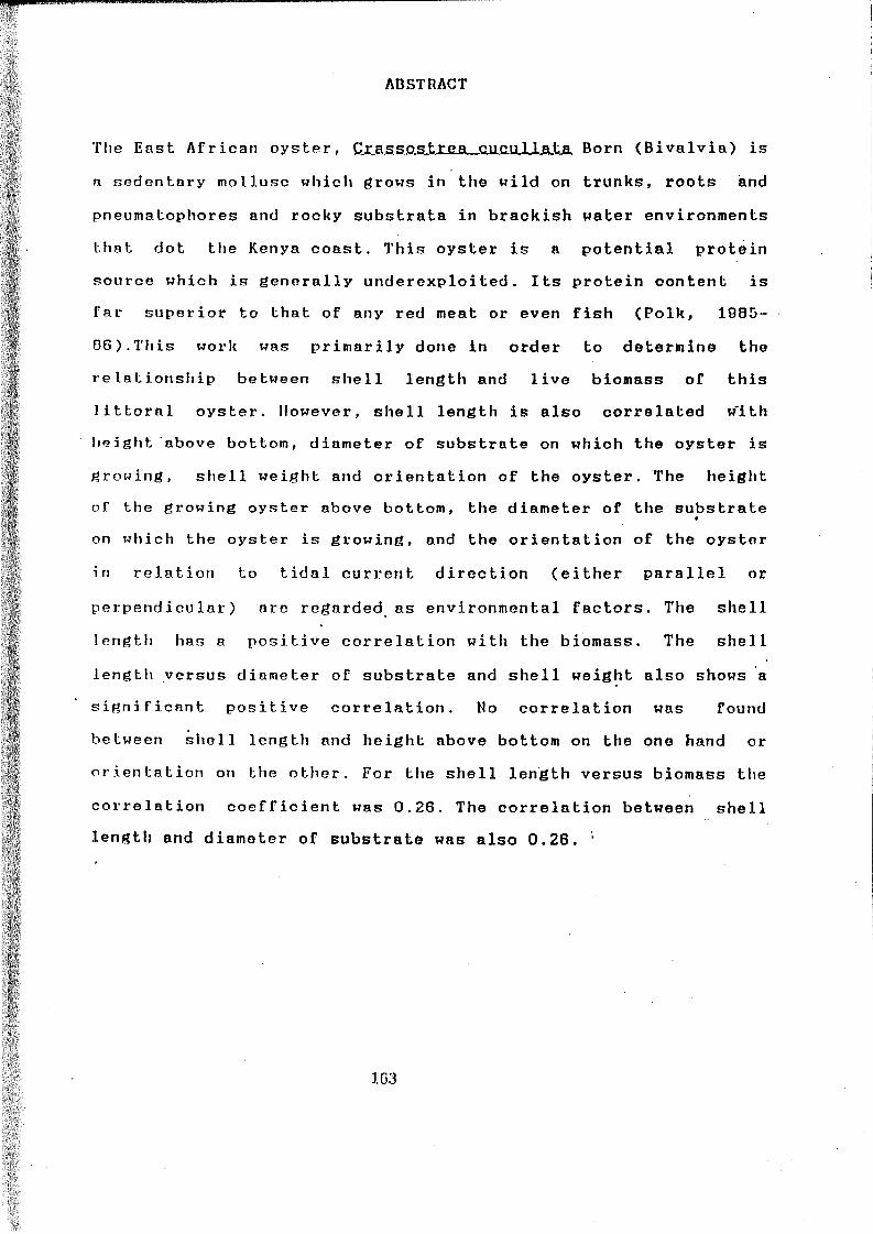
ABSTRACT
The East African oyster, Crassostrea cucullata Born (Bivalvia) is
a sedentary mollusc which grows in the wild on trunks, roots and
pneumatophores and rocky substrata in brackish water environments
that dot the Kenya coast. This oyster is a potential protein
source which is generally underexploited. Its protein content is
far superior to that of any red meat or even fish (Polk, 1985-
06).This work was primarily done in order to determine the
relationship between shell length and live biomass of this
littoral oyster. However, shell length is also correlated w'ith
height above bottom, diameter of substrate on which the oyster is
growing, shell weight and orientation of the oyster. The height
of the growing oyster above bottom, the diameter of the substrate«
on which the oyster is growing, and the orientation of the oyster
in relation to tidal current direction (either parallel or
perpendicular) are regarded as environmental factors. The shell
length has a positive correlation with the biomass. The shell
lengtli versus diameter of substrate and shell weight also shows a
significant positive correlation. No correlation was found
between shell length and height above bottom on the one hand or
orientation on the other. For the shell length versus biomass the
correlation coefficient was 0.26. The correlation between shell
.length and diameter of substrate was also 0.26. 1
103

5. OTHER ACTIVITIES
The project is actively participating in the organization of an International symposium and workshop " Status and future of Large Marine Ecosystems (LME) of the Indian Ocean.The project has also been further involved in the start, although on a very small scale of a commercial oyster farming at Gazi: different new racks have been build and the oysters are settling naturally on the substrata. It is planned to start a large scale oyster farm in the very near future ( see report J.Tack)The set up of an aquaculture section is aimed. At present fish are being raised in the fish ponds of the Institute (see report on aquaculture). One of the researchers is seriously interested in doing research on prawn culturing.
164

6. CONCLUSION
The research is proceeding very well. The sampling are being done on a regular basis and the necessary analyzing equipment is available.When overviewing the research results from the past year, one can note some important achievements.The results from the research on the Mangrove ecosystem in Gazi allowed one to obtain a better understanding of some important ecological compartments: Mangrove trees, phytoplankton, Zooplankton, fish, bacteria and nutrients. Data are available on mangrove biomass levels, biomass increments, litterfall, littercomposition and litterdecomposition. Within the pelagic creek ecosystem, information has been obtained on community composition and species diversity for Zooplankton, phytoplankton and fish.Biomass levels and/or activities of the pelagic compartments (phytoplankton, Zooplankton, fish, bacteria) were evaluated over a one year cycle and compared to the environmental abiotic factors (temperature, salinity, oxygen, nutrients) simultaneously measured. The benthic community at Gazi was also studied ; data are available on the distribution and cover of benthic algae and on the abundance and diversity of marine Harbacticoids. More results on zoobenthos will be available soon in the frame of a Masters' thesis at the State University of Ghent. Although it is too early for a synthesis of the ecological functioning of the Kenyan Mangrove ecosystem, it seems obvious that at least part of the ecological puzzle is being unravelled.The results on the diversity and cover of marine algae and corals along the Kenyan coast are very important from a conservation and economic viewpoint. More data on coral species diversity, growth and age will be available soon, in the frame of. a Masters' thesisfor the FAME course.The assessment of the pollution impact in the area around Mombasa has started; the first basic data on landbased pollution sources and loads have been compiled. A set of data on degradable organic materials and microbial pollution, is available for Tudor creek, covering a one years cycle. These and other environmental parameters ( Temperature, pH, Oxygen, POC, ...) have been, orwill be measured soon, in the creeks around Mombasa and in theMombasa coastal area.The positive evolution of the projects (VLIR and EEC) is furthermore being reflected in the increasing number of organizations and researchers visiting the projects at the Kenya Marine and Fisheries Research Institute.
165

7.APPENDIX
List of main addresses :
Delta Institute for Hydrobioiogical ResearchVierstraat 28, 4401, EA Yerseke, The Netherlands
Phone: 31/1131/1920 Fax : 31/1131/3616
Catholic University of NijmegenLaboratory of Aquatic Ecology
Tooernooiveld, 6525 ED Nijmegen, The Netherlands Phone : 31/80/652493
Fax : 31/80/553450
Kenya Marine and Fisheries Research InstituteP.O.Box 81651, Mombasa, Kenya
Phone : 254/11/472270 Fax : 254/11/472270
Nairobi UniversityZoology Department
P.O.Box 30197 Nairobi, Kenya
Phone : 254.2.43720
Rijksuniversiteit GentLedeganckstraat 35 B-900 Gent, Belgium
Sektie Mariene Biologie Phone : 32/91/645210
Fax : 32/91/205083 Sektie Plantkunde
Phone : 32/91/645058 Fax : 32/91/205083
Vrije Universiteit BrusselPleinlaan 2, B-1050 Brussels, Belgium
Dienst ECOL Phone : 32/2/641.34.09 or 641.34.04
Fax : 32/2/641.34.03 Dienst ANCH
Phone : 32/2/641.32.63 Fax : 32/2.641.34.03
166