Embed Size (px)
Citation preview

KAUNAS UNIVERSITY OF TECHNOLOGY
FACULTY OF ELECTRICAL AND ELECTRONICS ENGINEERING
Harsh Patel
OPTIMAL POWER SHARING IN MICROGRID
Master’s Degree Final Project
Supervisor
Prof. Dr. Saulius Gudžius
KAUNAS, 2017
KAUNAS UNIVERSITY OF TECHNOLOGY
FACULTY OF ELECTRICAL AND ELECTRONICS ENGINEERING
DEPARTMENT OF ELECTRIC POWER SYSTEMS
OPTIMAL POWER SHARING IN MICROGRID
Master’s Degree Final Project
Electrical Energy Engineering (Code 621H63003)
Supervisor
Prof. dr. Saulius Gudžius
05/06/2017
Reviewer
Assoc. prof. Gytis Svinkūnas
05/06/2017
Project made by
Harsh Patel
KAUNAS, 2017
KAUNAS UNIVERSITY OF TECHNOLOGY
Electrical and Electronics Engineering
(Faculty)
Harsh Patel
(Student's name, surname)
Electrical Power Engineering - 621H63003
(Title and code of study programme)
"Optimal Power Sharing in Microgrid"
DECLARATION OF ACADEMIC INTEGRITY
26
May
2017
Kaunas
I confirm that the final project of mine, Harsh Patel, on the subject “Optimal Power Sharing
in Microgrid” is written completely by myself; all the provided data and research results are correct
and have been obtained honestly. None of the parts of this thesis has been plagiarised from any
printed, Internet-based or otherwise recorded sources. All direct and indirect quotations from
external resources are indicated in the list of references. No monetary funds (unless required by
law) have been paid to anyone for any contribution to this thesis.
I fully and completely understand that any discovery of any manifestations/case/facts of
dishonesty inevitably results in me incurring a penalty according to the procedure(s) effective at
Kaunas University of Technology.
(name and surname filled in by hand) (signature)
Harsh Patel. OPTIMAL POWER SHARING IN MICROGRID: Master‘s thesis in
Electrical Power Engineering/supervisor Prof. Dr Saulius Gudzius. Kaunas University of
Technology, Faculty of Electrical and Electronics Engineering, Department of Electrical Power
Engineering.
Research area and field: Electrical and Electronics Engineering, Technological Sciences
Keywords: Microgrid, Power sharing, optimal load, Demand side response, Load sharing
Kaunas, 2017. 61 p.
SUMMARY
Internationally, power demand is booming so, renewable energy based distributed generator and
Microgrid spider network will increasingly play a decisive role in electricity production,
distribution and most advantageous level power sharing. A Microgrid comprises of various sort
of load and disseminated generators that work as a solitary controllable framework. Presently a
day, control gadgets are on edge about wellbeing when the utility network associated with
Microgrid or other inexhaustible assets at interconnected or islanded mode.
The main goal of this thesis is to inspect and propose using a multi-input DC-DC power
converter for grid connected hybrid Microgrid system to reduce the cost and share the power at
optimal level. In the system, it consists of the multi-input DC-DC converter and full-bridge DC-
AC IGBT inverter. If the fluctuation is more in the output of renewable energy resources than
maximum power point tracking algorithm is used by input sources of PV and the wind. The
integration of DC bus and Hybrid Microgrid renewable power supply system implemented and
simulated using MATLAB/SIMULINK as compared to use directly AC bus. Methods that have
been used to control stability in Microgrid by load sharing are analysed in this thesis. Also in this
thesis, a price-based demand response is proposed using to share power in Microgrid. By utilizing
this technique it is less demanding to keep up security amongst request and era. It is an imperative
about dynamic and receptive power control in the power framework, particularly when the diverse
sort of Microgrid sustainable power source assets associated with the utility network. As a result,
how the modelling of the power grid infrastructure with Microgrid connected renewable energy
resources are controlled and discussed here and the result of controlling load, frequency, voltage
and current are achieved here. On the basis of parameters results the power sharing is possible at
optimal level with system balancing and reduce the cost.

Harsh Patel. OPTIMALUS GALIOS PASKIRSTYMAS MIKROTINKLE.
Elektros energetikos inžinerijos magistro baigiamasis projektas / vadovas prof. dr. Saulius
Gudžius; Kauno technologijos universitetas, Elektros ir elektronikos fakultetas, Elektros
energetikos sistemų katedra.
Mokslo kryptis ir sritis: Elektros ir elektronikos inžinerija, Technologiniai mokslai
Reikšminiai žodžiai: Mikro tinklelio, valdžios pasidalijimo, optimalus krūvis, paklausos
atsakymas, keliamoji dalijimasis.
Kaunas, 2017. 61 p.
SANTRAUKA
Didėjant energijos paklausai pasauliniu mastu, atsinaujinančiąja energetika paremtos paskirstytųjų
generatorių ir mikrotinklų sistemos vaidina vis svarbesnį vaidmenį elektros energijos gamyboje ir
optimaliam paskirstyme. Mikrotinklas susideda iš įvairios rūšies apkrovų ir paskirstytųjų
generatorių, kurie veikia kaip viena valdoma sistema. Dabartiniu metu iškyla galios elektronikos
įrenginių apsaugos problemos, kai skirstomieji tinklai sujungiami su mikrotinklais,
atsinaujinančiaisiais šaltiniais arba autonominiais tinklais.
Šio darbo tikslas yra ištirti ir pasiūlyti naudoti daugelio įėjimų NS-NS keitiklį prie
tinklo prijungtai hibridinio mikrotinklo sistemai, sumažinantį išlaidas ir optimaliai paskirstanti
energiją. Sistemą sudaro daugelio įėjimų NS-NS keitiklis ir tiltelinis NS-KS IGBT inverteris. Jei
nuokrypiai yra ryškesni atsinaujinančių šaltinių energijos gamyboje, maksimalios galios sekimo
algoritmą taiko fotovoltinių ir vėjo maitinimo šaltiniai. Sistemos modelis sudarytas
MATLAB/SIMULINK programoje. Modeliuojant yra naudojamas maksimalios galios sekimo
algoritmas tokiems šaltiniams kaip: saulės elementai ar vėjo generatoriai, kai jų laidumo
svyravimai yra dideli. Darbe yra apžvelgti ir išanalizuoti mikrotinklo stabilumo valdymo metodai
paskirstant apkrovą. Darbe taip pat siūlomas kaininis elektros energijos paklausos valdymas,
paskirstant energiją mikrotinkle. Naudojant šį metodą yra paprasčiau palaikyti stabilumą tarp
vartojimo ir generavimo. Kaip rezultatas, kaip iš elektros tinklo infrastruktūrą su Microgrid
modeliavimas prijungtas atsinaujinantys energijos ištekliai yra valdomi ir čia aptariama ir
kontroliuoti krovinio, dažnio, įtampos ir srovės rezultatas pasiekiamas čia. Dėl parametrus
rezultatų pagrindu valdžios pasidalijimo yra įmanoma optimalaus lygio su sistemos balansavimo
ir sumažinti išlaidas.
CONTENTS
LIST OF FIGURES………………………………………………………………………………8
LIST OF TABLES……………………………………………………………………….…….....9
LIST OF GRAPHS……………………………………………………………………………….9
ABBREVIATION AND SYMBOLS INTERPRETATION DICTIONARY…………………...10
ABSTRACT…………………………………………………………….………………….……12
INTRODUCTION……………………………………………………………………………….13
1 Overview of Microgrid........................................................................................................... 15
1.1 Microgrid model used for demonstrations – represent DOD facility (department of
defence) ...................................................................................................................................... 15
1.2 Working of Microgrid ..................................................................................................... 16
1.3 Microgrid as spider network ........................................................................................... 16
1.4 Spider network of Microgrid and utility interconnected ................................................ 19
1.5 How the power sharing in the grid? ................................................................................ 23
1.6 What is the load shedding? ............................................................................................. 23
2 Concept of power sharing based on load demand .................................................................. 24
2.1 Power sharing technique in grid ..................................................................................... 25
2.2 Overview of Microgrid controls and modes ................................................................... 26
2.2.1 Grid connected mode ............................................................................................... 27
2.2.2 Islanded mode .......................................................................................................... 27
2.2.3 Seamless transfer ..................................................................................................... 27
2.3 Droop control .................................................................................................................. 27
2.4 Power sharing for a Microgrid with MDG ..................................................................... 28
3 Microgrid concept .................................................................................................................. 29
3.1 Frequency stabilisation in power sharing ....................................................................... 29
3.2 Difficulties for power sharing in Microgrid ................................................................... 30
3.3 How does Microgrid connect to main grid? ................................................................... 31
3.3.1 Why would everybody choose to connect to Microgrids? ...................................... 31
3.3.2 How much can a Microgrid power? ........................................................................ 32
4 Energy demand side management .......................................................................................... 33
4.1 Demand response ............................................................................................................ 33
4.2 Load side response .......................................................................................................... 34
4.2.1 Power Generation .................................................................................................... 34
4.2.2 Electricity distribution ............................................................................................. 34
4.3 Operating principles of load management ...................................................................... 34
4.4 Advantages of Deregulation ........................................................................................... 35
4.5 Power factor improvement and penalty factor ................................................................ 36
4.5.1 Why should improve the power factor? .................................................................. 36
4.5.2 Reduces loading on transformers ............................................................................ 37
4.5.3 Power factor improvement methods ........................................................................ 37
4.5.4 Disadvantages of lower power factor ...................................................................... 37
5 Availability based tariff - ABT .............................................................................................. 38
5.1 Working operation of ABT ............................................................................................. 39
5.2 ABT feature .................................................................................................................... 39
5.3 How ABT actively encourage trading? .......................................................................... 39
5.4 Unscheduled Interchange (U.I) ....................................................................................... 40
5.5 Category for open access [53] ........................................................................................ 41
5.5.1 Research and development about Microgrid ........................................................... 41
6 The Wind and photovoltaic resources connected to MI CUK DC to DC converter
technology in microgrid ................................................................................................................ 42
6.1 Working principle ........................................................................................................... 42
7 Demand-side energy management ......................................................................................... 48
7.1 Algorithm of automatic demand response ...................................................................... 50
7.2 Price based demand response.......................................................................................... 52
7.2.1 Methodology and proposed algorithms ................................................................... 52
7.3 Simulation results ........................................................................................................... 53
7.4 Overall results ................................................................................................................. 54
8 Internal stability margin and frequency ramp rates in Microgrid. ......................................... 55
8.1 Impact on transformer due to PV in Microgrid .............................................................. 57
8.2 Load frequency control on generation side ..................................................................... 58
9 Conclusions ............................................................................................................................ 61
10 References .......................................................................................................................... 62
11 APPENDIXES .................................................................................................................... 66
11.1 APPENDIX - 1 Converter structure and graphical data ................................................. 66
11.2 APPENDIX – 2 Programming and readings .................................................................. 75
LIST OF FIGURES
Figure 1.1 Microgrid DOD model [5] ........................................................................................... 15
Figure 1.2 Local (Public) grid connected with Microgrid [12] ..................................................... 18
Figure 1.3 Microgrid connected with utility grid spider network [5] ........................................... 19
Figure 1.4 Results of fuel consumption Vs load [5] ...................................................................... 19
Figure 1.5 Utility power cable with Microgrid location [5] .......................................................... 20
Figure 1.6 Utility grid operation behaviour with Microgrid [5] .................................................... 21
Figure 1.7 Standalone system for power sharing and standby usage [44] .................................... 23
Figure 2.1 System structure of load shading [45] .......................................................................... 24
Figure 2.2 Standby and load sharing technique ............................................................................. 26
Figure 2.3 Active power and frequency drop characteristics ........................................................ 28
Figure 3.1 Basic block diagram of Microgrid [47] ........................................................................ 29
Figure 3.2 Meter of frequency stability limit [48] ......................................................................... 30
Figure 3.3 Microgrid with interconnected - decentralising open power market [46].................... 31
Figure 3.4 Example of Microgrid at "SANTA RITA JAIL - CALIFORNIA" [49] ...................... 32
Figure 4.1 Effect of demand side management system due to load [28]....................................... 34
Figure 4.2 Difference between regulation and deregulation [51] .................................................. 35
Figure 4.3 Power factor triangle [55] ............................................................................................ 36
Figure 5.1 Generation availability layout / 15-minute power block lockdown system [52] ......... 38
Figure 5.2 Open access model [53] ............................................................................................... 41
Figure 6.1 Microgrid with MI CUK converter and utility ............................................................. 42
Figure 7.1 Demand responds control flow .................................................................................... 48
Figure 7.2 Algorithms of automatic demand respond [22] ........................................................... 50
Figure 7.3 Types of demand response [13] ................................................................................... 52
Figure 7.4 Priority control flow chart [13] .................................................................................... 53
Figure 7.5 Simulation diagram and appliance priority table [13].................................................. 53
Figure 8.1 Ice landed Microgrid - frequency deviation [4] ........................................................... 55
Figure 8.2 Proposed model of standalone PV Microgrid with utility ........................................... 57
Figure 8.3 Load frequency control mechanism [54] ..................................................................... 59
Figure 11.1Basic CUK converter circuit ....................................................................................... 66
Figure 11.2 Ideal switching operation ........................................................................................... 67
Figure 11.3 Converter circuit from model ..................................................................................... 67
Figure 11.4 Schematic diagram of CUK converter ....................................................................... 68
Figure 11.5 Similarity of cascaded boost and buck converter ....................................................... 69
Figure 11.6 Similarity with CUK converter .................................................................................. 69
Figure 11.7 Voltage and current waveform analysis ..................................................................... 71
Figure 11.8 Power exchange data for ABT and U.I - 28/05/2017................................................. 76
LIST OF TABLES
Table 1.1 Types of Microgrid [13] ................................................................................................ 22
Table 2.1 Parameters required in Microgrid for power sharing .................................................... 25
Table 7.1 Data of six buses and three generator system for 24 hours [22] ................................... 51
Table 7.2 Allotted start hour for various loads [22] ...................................................................... 52
Table 7.3 Old and new load curve data for six buses. [22] ........................................................... 52
Table 11.1 Rated parameters of model .......................................................................................... 74
Table 11.2 U.I rate with frequency ................................................................................................ 75
LIST OF GRAPHS
Graph 6.1 Voltage comparison (without-with) ............................................................................. 43
Graph 6.2 Current comparison (without-with) .............................................................................. 44
Graph 6.3 Converter output voltage, AC side supply voltage and DC bus voltage ...................... 45
Graph 6.4 Current of battery and charge controller on bus ........................................................... 45
Graph 6.5 Three phase voltage and current ................................................................................... 45
Graph 6.6 Active and reactive power ............................................................................................ 46
Graph 6.7 Active and Reactive power development [3] ............................................................... 47
Graph 7.1 Six buses and three generator system measurement ..................................................... 51
Graph 7.2 Results of load profile [13] ........................................................................................... 54
Graph 8.1 Solar irradiance ramps [4] ............................................................................................ 55
Graph 8.2 Ramp rates frequency decay and magnitude [4] .......................................................... 56
Graph 8.3 Frequency ramp rates and system inertia [4] ................................................................ 56
Graph 8.4 Consumption of solar and grid of 12 house within 24 hours ....................................... 58
Graph 8.5 Comparison between without LFC and with LFC ....................................................... 60
Graph 11.1 Battery current with charge controller – (before-after) .............................................. 71
Graph 11.2 PV – voltage with converter - (before-after) .............................................................. 72
Graph 11.3 Wind technical data output after PMSG - (before-after) ............................................ 72
Graph 11.4 Wind generator terminal voltage after rectifier - (before-after) ................................. 72
Graph 11.5 Battery voltage, current and SOC% ........................................................................... 73
Graph 11.6 Battery discharging characteristics and generator terminal FFT analysis .................. 73

10
ABBREVIATION AND SYMBOLS INTERPRETATION DICTIONARY
ABBREVIATIONS
OPF: Optimal power flow
DG: Distributed generator
UPC: Unit power flow
FCC: Feeder flow control
PCC: Point of common coupling
DOD: Department of defence
SPIDERS: Smart power infrastructure demonstration and energy reliability and security
DERS: Distributed energy resources
STATCOM: Static synchronous compensator
STS: Static Transfer Switch
CHP: Combined heat and power
PV: Photovoltaic
VSC: Voltage source converter
FC: Fuel cells
CERTS: Consortium for electric reliability technology solutions
EFA: Electricity forward agreement
DISCOMS: Distribution companies
PPA: Power purchase agreement
EPA: Energy purchase agreement
ABT: Availability best tariff
CERC: Central electricity regulatory commission
SLDC: State load dispatch centre
RLDC: Regional load dispatch centre
IEGC: Indian electricity grid code
SEB: State electricity board
UI: Unscheduled Interchange
LFC: Load frequency control
AGC: Automatic generation control
FMGO: Free governor mode of operation
DR: Demand response
TOU: Time of unit
RMU: Ring main unit

11
SYMBOLS
R = Regulating contestant
Te = Output electrical torque
Tm = Mechanical input torque
f = Frequency
(∆𝑃𝑟𝑒𝑓) = Negative slop difference
t = Time
DLt = Dispatchable Load at hour t
TLt = Sum of load at hour t
fc = Fuel cost
Pgmin, Pgmax = Generator limit minimum and maximum
∝ 𝑖, 𝛽𝑖, 𝛾𝑖 = Arbitery constant
Pgi = Cost of power produced at generator i
∑ 𝑃𝑔𝑖𝑘𝑛 = Total power received by load
𝜔 ∗ = Active power
e* = Reactive power
m,n = Slopes

12
ABSTRACT
Internationally, power demand is booming so, renewable energy based distributed generator and
Microgrid spider network will increasingly play a significant role in electricity production,
distribution and most advantageous level power sharing. A Microgrid consists of different kind of
load and distributed generators that operate as a single controllable system. Now a day, power
electronics devices are anxious about safety when the utility grid connected with Microgrid or
other renewable resources at interconnected or islanded mode.
The main goal of this thesis is to inspect and propose using a multi-input DC-DC power
converter for grid connected hybrid Microgrid system to reduce the cost and share the power at
optimal level. In the system, it consists of the multi-input DC-DC converter and full-bridge DC-
AC IGBT inverter. If the fluctuation is more in the output of renewable energy resources than
maximum power point tracking algorithm is used by input sources of PV and the wind.
Generally, in the interconnected power system especially when the renewable energy
resources are connected with utility it is most important to maintain active and reactive power
because the renewable sources depend on nature. So that for precaution, here in the model there is
battery storage unit is deployed nearest to DC bus, which helps in the poor voltage condition. It is
also possible to control reactive power by main utility grid DGs, but the first priority is from
Microgrid sources. This makes the system efficient and reliable. So in the graphs, it is clearly
shown that when the Microgrid output is not constant then the battery storage unit and DGs are
controlled the active and reactive power in the system. The DC-DC CUK converter gives the
benefits to boost up the voltage on DC bus. Also, there is a difference between without and with
the converter is showing in the graph.
Here in the model, we proposed to use SPIDER network because it helps to make a system
more reliable and efficient. General interconnected network was totally affected when the grid
goes down, but if different renewable sources are connected together and make an Autonomous
Microgrid network which is helpful to give support to another system in an emergency condition
or to maintain the frequency stabilisation also. Collecting power from Microgrid first to DC bus
also gives advantages because when the different sources are injecting AC to the grid directly it is
a huge impact on utility grid network like stress and overloaded sometimes. If there is a change in
input on DC bus, but with the help of special VSCs the output of AC is constant and reduce the
losses and improve the voltage regulation to make the grid in the discipline.
13
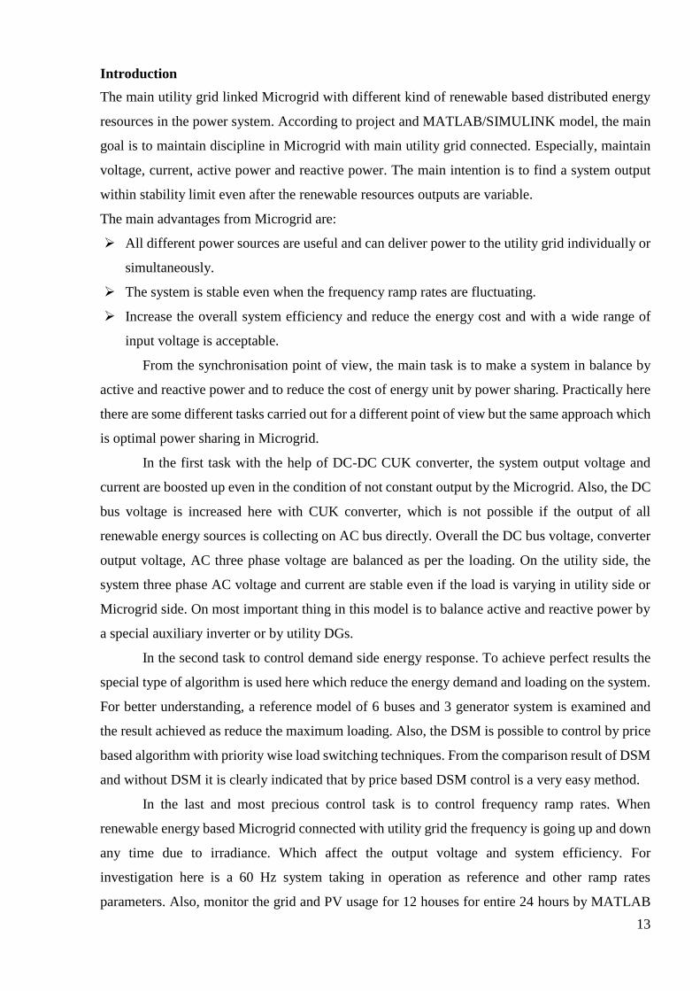
Introduction
The main utility grid linked Microgrid with different kind of renewable based distributed energy
resources in the power system. According to project and MATLAB/SIMULINK model, the main
goal is to maintain discipline in Microgrid with main utility grid connected. Especially, maintain
voltage, current, active power and reactive power. The main intention is to find a system output
within stability limit even after the renewable resources outputs are variable.
The main advantages from Microgrid are:
All different power sources are useful and can deliver power to the utility grid individually or
simultaneously.
The system is stable even when the frequency ramp rates are fluctuating.
Increase the overall system efficiency and reduce the energy cost and with a wide range of
input voltage is acceptable.
From the synchronisation point of view, the main task is to make a system in balance by
active and reactive power and to reduce the cost of energy unit by power sharing. Practically here
there are some different tasks carried out for a different point of view but the same approach which
is optimal power sharing in Microgrid.
In the first task with the help of DC-DC CUK converter, the system output voltage and
current are boosted up even in the condition of not constant output by the Microgrid. Also, the DC
bus voltage is increased here with CUK converter, which is not possible if the output of all
renewable energy sources is collecting on AC bus directly. Overall the DC bus voltage, converter
output voltage, AC three phase voltage are balanced as per the loading. On the utility side, the
system three phase AC voltage and current are stable even if the load is varying in utility side or
Microgrid side. On most important thing in this model is to balance active and reactive power by
a special auxiliary inverter or by utility DGs.
In the second task to control demand side energy response. To achieve perfect results the
special type of algorithm is used here which reduce the energy demand and loading on the system.
For better understanding, a reference model of 6 buses and 3 generator system is examined and
the result achieved as reduce the maximum loading. Also, the DSM is possible to control by price
based algorithm with priority wise load switching techniques. From the comparison result of DSM
and without DSM it is clearly indicated that by price based DSM control is a very easy method.
In the last and most precious control task is to control frequency ramp rates. When
renewable energy based Microgrid connected with utility grid the frequency is going up and down
any time due to irradiance. Which affect the output voltage and system efficiency. For
investigation here is a 60 Hz system taking in operation as reference and other ramp rates
parameters. Also, monitor the grid and PV usage for 12 houses for entire 24 hours by MATLAB

14
programming. From the graph, it gives an idea of usage of utility and Microgrid and to control
frequency ramp rates timing. To solve that problem we proposed to use LFC system here. This is
done by feedback control loop in Microgrid with utility power system. From the graph, by load
frequency control system the frequency fluctuation is controlled in a short time and avoids the
system collapse and cascade tripping.

15
1 Overview of Microgrid
What is Microgrid?
“A various group of distributed energy resources which are interconnected and it clearly specifies
an electrical border limits and acts as a single controllable entity with respect to the grid is defined
as Microgrid”. It is capable of linking and disconnect from the main grid and operates either grid
connected or island mode. It is a local energy grid which gives main advantages to detach from
the main grid and run as an entity [40].
What is power sharing?
It is an electrical event, which can divide the power between two separate systems when it should
be required or any repair, maintenance or power outage condition. It also helps to mitigate the
demand of suddenly increased load in a peak time. Power sharing depends on different methods
and different types with bulk amount of electricity. Power is coming from different kind of power
station and substation which includes conventional and non-conventional sources [40].
Overview of power grid & transmission sharing
What is a “Grid”?
An Interconnected power system which covers a major portion of a country’s territory or state is
called a Grid. Different states grid might be interconnected and to make a central grid.
What is an “Interconnection” network?
Two or more generating stations are interconnected by tie lines to form an interconnection.
Interconnection provides the best use of power resources and ensures greater security of supply
and maintenance.
1.1 Microgrid model used for demonstrations – represent DOD facility (department of
defence)
Figure 1.1 Microgrid DOD model [5]

16
As for showing in above model that each premise has been connected to common grid line network
and with an isolated switch so that it operates by its own power substation. If there is a problem
occurring anywhere in a grid network, then other peak load station take over that load and continue
the operation. Moreover, when the fault occurred then it isolated by self and operated the isolated
grid. There is one important thing in Microgrid is that every power generation sources have a
storage unit that helps it to start up in blackout condition or ignition power to another grid for start-
up [5].
Difference between smart grid and Microgrid
A variety of manifold loads and circulated energy resources are operated in parallel with the
periphery of utility grid or any independent power system that is Microgrid. It increases the
reliability with distributed generation, increases efficiency with reduced transmission length, and
easier integration of alternative energy sources. On another side, the brilliant matrix is entirely
unexpected, as a result of the exceptionally current development. It is turning out to the electrical
network and uses correspondence innovation and data as a specialist organisation. It is given and
checking the data like load conduct, productivity, unwavering quality, financial aspects, generation
and conveyance [41].
1.2 Working of Microgrid
All structures are associated by utility lattice to focal power sources, which enable us to utilise any
sort of apparatus. However, without interconnected implies that when some portion of the matrix
should be repaired so around then everybody is influenced because of it. In this out of order time,
Microgrid provides a support to the network. In this out of request time, Microgrid gives a support
to the system. A Microgrid can be controlled by disseminated generators, batteries, and
inexhaustible assets like sun oriented boards relying upon how it is fuelled and its accessibility
and how its necessities.
1.3 Microgrid as spider network
The Smart Power Infrastructure Demonstration and Energy Reliability and Security (SPIDERS)
technology are to maintain operational surety through trusted, reliable, and resilient electric power
generation and distribution on military installations. SPIDERS are standardisation of the design
structure and network which is supporting in Microgrid for future applications [4] [5].
The project will promote adoption of Microgrid technology for the energy surety Microgrid design
process that focuses on:
Energy dependability for significant missions
High readiness and immediately deployable technologies
Cybersecurity for the control systems
17
Local control of Microgrid resources enables smart grid functionality, including:
Demand response - shutting down high energy use appliances such as air conditioners for
few hours during the high peak time of electricity.
The distributed energy resources interconnection and integration including generators, PV
panels, and small wind turbines.
Net metering - Microgrid is capable of selling power to utility give back or else in the main
utility bills they give back money rebate.
Two primary points of interest about a run of the mill Microgrid arrangement:
ESM Microgrid configuration permits the Microgrid to be matrix tied worked in
conjunction with, and notwithstanding expanding, the primary network with Microgrid-
produced power; or else to be islanded worked totally autonomous of the principle control
lattice.
Computer demonstrating that uses broad examination capacities to decide the most
productive, most savvy, most secure and most secure blend of circulated vitality assets
(DERs) inside the Microgrid.
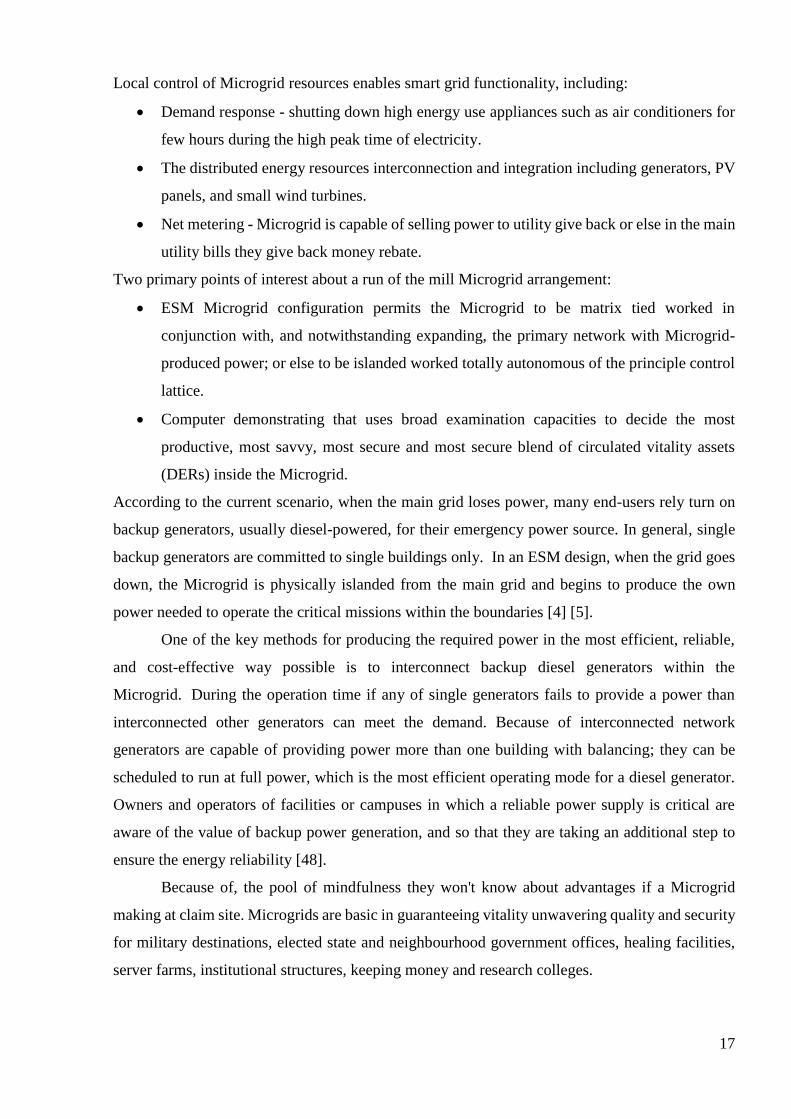
According to the current scenario, when the main grid loses power, many end-users rely turn on
backup generators, usually diesel-powered, for their emergency power source. In general, single
backup generators are committed to single buildings only. In an ESM design, when the grid goes
down, the Microgrid is physically islanded from the main grid and begins to produce the own
power needed to operate the critical missions within the boundaries [4] [5].
One of the key methods for producing the required power in the most efficient, reliable,
and cost-effective way possible is to interconnect backup diesel generators within the
Microgrid. During the operation time if any of single generators fails to provide a power than
interconnected other generators can meet the demand. Because of interconnected network
generators are capable of providing power more than one building with balancing; they can be
scheduled to run at full power, which is the most efficient operating mode for a diesel generator.
Owners and operators of facilities or campuses in which a reliable power supply is critical are
aware of the value of backup power generation, and so that they are taking an additional step to
ensure the energy reliability [48].
Because of, the pool of mindfulness they won't know about advantages if a Microgrid
making at claim site. Microgrids are basic in guaranteeing vitality unwavering quality and security
for military destinations, elected state and neighbourhood government offices, healing facilities,
server farms, institutional structures, keeping money and research colleges.

18
Figure 1.2 Local (Public) grid connected with Microgrid [12]
General straightforward and single-site reinforcement era to consolidate appropriated era,
stack administration, and dynamic communication with the utility, Microgrids serves to
associations to keep up vitality framework, enhance unwavering quality, and secure against
expansive disturbances on the fundamental lattice. [12].
Official definition of Microgrid
“A different bunch of interconnected loads and distributed energy resources within particular
electrical limits that perform as a single controllable unit with respect to the grid and can also
connect and disconnect from the grid to enable it to operate in both way grid-connected or island
mode.”
Common features
Decoupling of generators from loads
Flawless transitions to/from utility
Common benefits:
Operators awareness
Combination of renewable energy resources
Multiple modes of operation
Assessment process:
Recognise all sources of power and which one to be served
To find critical situation of each load and capabilities of each resource
Requirements of interconnection for utility
Distribution system:
Identify points of common coupling with utility
Find out if seamless transition is required
Calculate of system components dynamic situation

19
Control system:
Estimate existing control system’s capabilities
Establish new control and data points
Resolve cyber security risks
1.4 Spider network of Microgrid and utility interconnected
Reduce diesel fuel consumption and increased reliability.
Any power sources become a SPIDERS generator.
Distribution control matching with generator load.
Dynamic electrical topology responds to system events.
The Microgrid relates to the utility grid in a spider network as shown below the network.
Figure 1.3 Microgrid connected with utility grid spider network [5]
Figure 1.4 Results of fuel consumption Vs load [5]
As it can see above example of spider Microgrid network with the utility grid, we reduce the fuel
consumption and increased the reliability. There are so many different types of benefits from the
spider network Microgrid. Now a day the government is supporting a project about Microgrid at
military base and defence organisation because they all are high demanding consumer and various
20
time base consumers of different loads so it is better to know and get perfect results of Microgrid
from them.
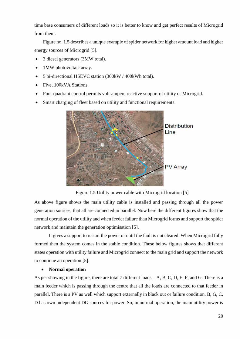
Figure no. 1.5 describes a unique example of spider network for higher amount load and higher
energy sources of Microgrid [5].
3 diesel generators (3MW total).
1MW photovoltaic array.
5 bi-directional HSEVC station (300kW / 400kWh total).
Five, 100kVA Stations.
Four quadrant control permits volt-ampere reactive support of utility or Microgrid.
Smart charging of fleet based on utility and functional requirements.
Figure 1.5 Utility power cable with Microgrid location [5]
As above figure shows the main utility cable is installed and passing through all the power
generation sources, that all are connected in parallel. Now here the different figures show that the
normal operation of the utility and when feeder failure than Microgrid forms and support the spider
network and maintain the generation optimisation [5].
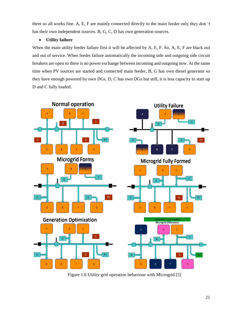
It gives a support to restart the power or until the fault is not cleared. When Microgrid fully
formed then the system comes in the stable condition. These below figures shows that different
states operation with utility failure and Microgrid connect to the main grid and support the network
to continue an operation [5].
Normal operation
As per showing in the figure, there are total 7 different loads – A, B, C, D, E, F, and G. There is a
main feeder which is passing through the centre that all the loads are connected to that feeder in
parallel. There is a PV as well which support externally in black out or failure condition. B, G, C,
D has own independent DG sources for power. So, in normal operation, the main utility power is
21
there so all works fine. A, E, F are mainly connected directly to the main feeder only they don ‘t
has their own independent sources. B, G, C, D has own generation sources.
Utility failure
When the main utility feeder failure first it will be affected by A, E, F. So, A, E, F are black out
and out of service. When feeder failure automatically the incoming side and outgoing side circuit
breakers are open so there is no power exchange between incoming and outgoing now. At the same
time when PV sources are started and connected main feeder, B, G has own diesel generator so
they have enough powered by own DGs. D, C has own DGs but still, it is less capacity to start up
D and C fully loaded.
Figure 1.6 Utility grid operation behaviour with Microgrid [5]
22
Microgrid forms
B and G operated by their own DGs on full power for their own purpose. Now generator D is
connected bidirectionally so D gives power to main load and utility feeder as well. But in this
condition, we can start up step by step all the loads not together all of them. So slowly increasing
generation and PV also support the feeder so now A, E and F are in operation.
Fully formed
Next step C is also connected and shared power bi-directional. So now all the loads are fully
worked and support to each other to balance a network. But in a meantime, we can focus on
operational cost and DG fuel because our main goal is to optimal power sharing. So, when do not
require unnecessary all the loads are disconnected from the main load and when the network is
stable and enough power than we disconnected first generator G. Still after disconnecting due to
spider network the system is stable.
Generator optimization
Now B & D is only bidirectional connected and PV increased the generation. So next generator C
also disconnected, because we can support an optimal way to power sharing and reduce overall
cost. Still, the system is stable in power spider network.
Microgrid differences
As mentioned before A, E, F is directly connected to main utility feeder only. C and D have own
DGs but not enough power. B and G have own enough capacity of DGs. So overall the figure
shows the differences what happened and affected when the Microgrid sources and renewable are
connected to Microgrid or without Microgrid. So, in this network with support by DGs and
renewable PV in spider network helps to B, C, D and G only. A, E, F are shut down totally when
feeder failure. These are the main benefits if A, E, F are also connected to spider network like
Microgrid self-independent sources or DGs than they have their own quick start up without losing
power.
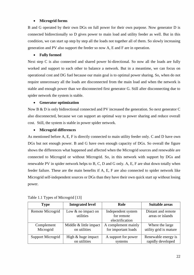
Table 1.1 Types of Microgrid [13]
Type Integrated level Role Suitable areas
Remote Microgrid Low & no impact on
utilities
Independent system
for remote
electrification
Distant and remote
areas or islands
Complement
Microgrid
Middle & little impact
on utilities
A complement mainly
for important loads
Where the large
utility grid is mature
Support Microgrid High & huge impact
on utilities
A support for power
systems
Renewable energy is
rapidly developed
23
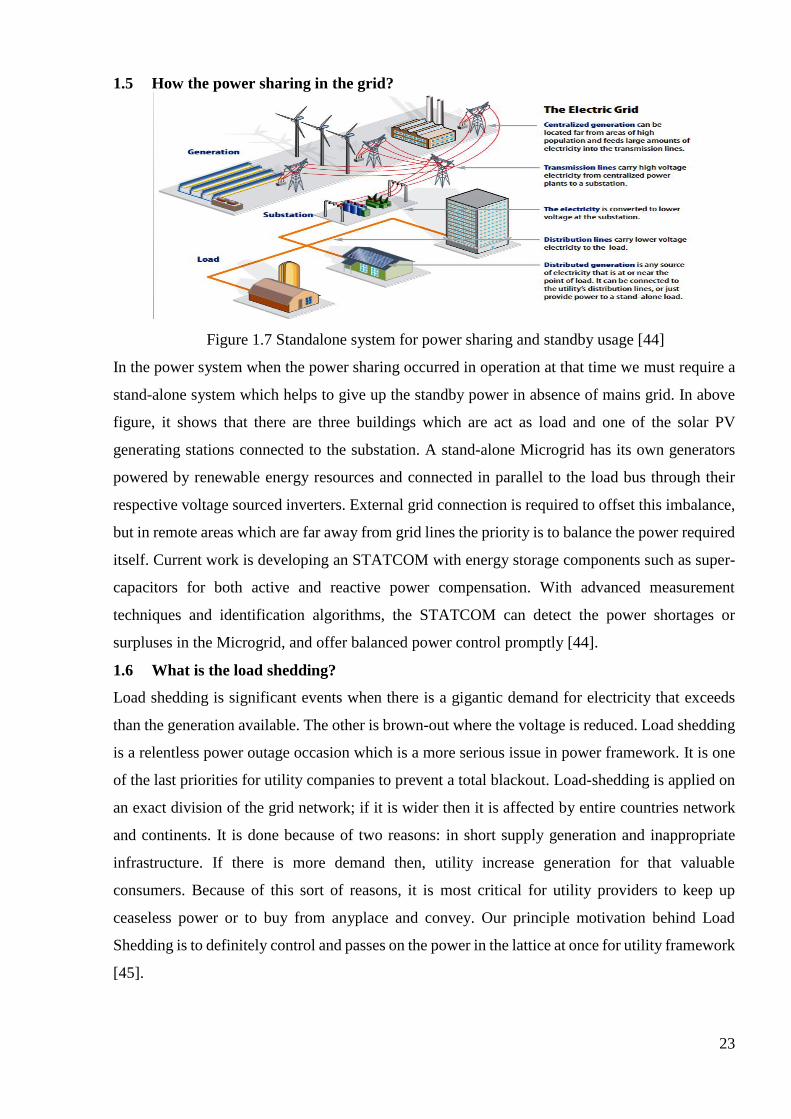
1.5 How the power sharing in the grid?
Figure 1.7 Standalone system for power sharing and standby usage [44]
In the power system when the power sharing occurred in operation at that time we must require a
stand-alone system which helps to give up the standby power in absence of mains grid. In above
figure, it shows that there are three buildings which are act as load and one of the solar PV
generating stations connected to the substation. A stand-alone Microgrid has its own generators
powered by renewable energy resources and connected in parallel to the load bus through their
respective voltage sourced inverters. External grid connection is required to offset this imbalance,
but in remote areas which are far away from grid lines the priority is to balance the power required
itself. Current work is developing an STATCOM with energy storage components such as super-
capacitors for both active and reactive power compensation. With advanced measurement
techniques and identification algorithms, the STATCOM can detect the power shortages or
surpluses in the Microgrid, and offer balanced power control promptly [44].
1.6 What is the load shedding?
Load shedding is significant events when there is a gigantic demand for electricity that exceeds
than the generation available. The other is brown-out where the voltage is reduced. Load shedding
is a relentless power outage occasion which is a more serious issue in power framework. It is one
of the last priorities for utility companies to prevent a total blackout. Load-shedding is applied on
an exact division of the grid network; if it is wider then it is affected by entire countries network
and continents. It is done because of two reasons: in short supply generation and inappropriate
infrastructure. If there is more demand then, utility increase generation for that valuable
consumers. Because of this sort of reasons, it is most critical for utility providers to keep up
ceaseless power or to buy from anyplace and convey. Our principle motivation behind Load
Shedding is to definitely control and passes on the power in the lattice at once for utility framework
[45].

24
2 Concept of power sharing based on load demand
Figure 2.1 System structure of load shading [45] According to figure 2.1 single diagram of a network that shows several chances for a load shedding
system to prevent a system collapse. As per the system diagram, buses D, E, F, and G are healthy
with grid tied (represented by A, B and C) for an islanding condition to occur. If the buses D, E,
F, and G are drawing power from the rest of the system then its loading impact is too heavy for
this time. Now assume lines A-D and B-D are on a common transmission tower and if a single
event like a tower failure took both lines out of service [45].
At the same time the heavy loading on system and two line loss. Now, line C-E is
overloaded, and that voltage in the system has emaciated. This loading is some extent. Assume,
generator E is little and not fit for neighbourhood stacking and that generator E tries to bolster
voltage and its field started to supply VARs past its long haul limit. System operators see the event
from a remote location where lines A-D and B-D were lost, and if the system was surviving but
less voltage. Then again, following few moments tap changers increment the voltage and
framework stack begin to increment. Two minutes after the occasion the field excitation limiter at
generator D compels the field to down and the voltage at the heaps falls again [45].
Then after one-minute tap changers start to raise load voltage again and load again rises.
Operators might see the heavy loading online C-E and become concerned but decided to accept
the condition. If they could monitor the generation and realise that the excitation limiters had
kicked in, they might even be more concerned. The protective relaying on the heavily overloaded
line C-E trips due to load violation that looks like a zone 3 distance fault. The system consisting
of buses D, E, F, and G has islanded with insufficient generation to support its load, several
minutes after the initial event. So in this critical situation frequency based load shedding is helpful
[45].
These conditions may system from unusually higher than forecasted demands that may be due to
the following:-
25
Unusual occasional changes,
Special occasions that may bring about loss of assorted qualities, and
Failure or overload of some elements in the facilities making up the supply system.
In the event that the supply transport has less voltage then, disengaging feeders for some brief
timeframe on the preset calendar. That is called as a "brownout" [45]. As a less than dependable
rule this two techniques connected together or well ordered and even after if the condition is wild
then, whole sub stations might be removed from administration incidentally or closed down. On
the off chance that it is over-burden and wild then a whole range may require a shutdown of the
framework included, an operation alluded to as "power outage” [45].
Brownouts have the potential to cause annoying occurrences such as erratic appliance
behaviour but can also cause serious damage to valuable electronics. Brownout is basically the
inverse as power surges. Additionally, rather than the voltage surging, the voltage hangs. Be that
as it may, brownouts are now and again critical for the service organisations for the power surges,
and by one means or another to avoid over-burdens, halting a potential power outage [45].
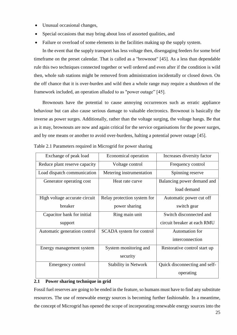
Table 2.1 Parameters required in Microgrid for power sharing
Exchange of peak load Economical operation Increases diversity factor
Reduce plant reserve capacity Voltage control Frequency control
Load dispatch communication Metering instrumentation Spinning reserve
Generator operating cost Heat rate curve Balancing power demand and
load demand
High voltage accurate circuit
breaker
Relay protection system for
power sharing
Automatic power cut off
switch gear
Capacitor bank for initial
support
Ring main unit Switch disconnected and
circuit breaker at each RMU
Automatic generation control SCADA system for control Automation for
interconnection
Energy management system System monitoring and
security
Restorative control start up
Emergency control Stability in Network Quick disconnecting and self-
operating
2.1 Power sharing technique in grid
Fossil fuel reserves are going to be ended in the feature, so humans must have to find any substitute
resources. The use of renewable energy sources is becoming further fashionable. In a meantime,
the concept of Microgrid has opened the scope of incorporating renewable energy sources into the
26
conventional grid, without a direct coupling with the conventional grid components. This is
possible due to the unique feature of a Microgrid, which allows both synchronised grid connected
operation and islanded operation in case of instabilities or power outages in the main grid or
blackout situation.
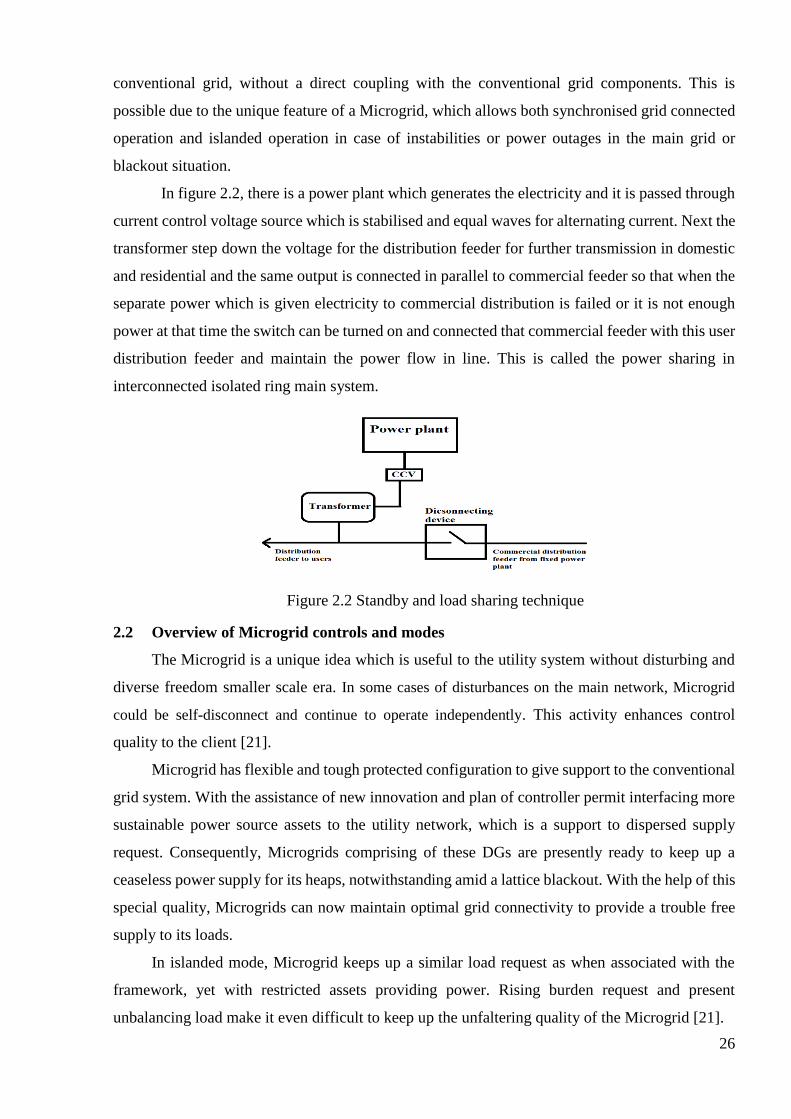
In figure 2.2, there is a power plant which generates the electricity and it is passed through
current control voltage source which is stabilised and equal waves for alternating current. Next the
transformer step down the voltage for the distribution feeder for further transmission in domestic
and residential and the same output is connected in parallel to commercial feeder so that when the
separate power which is given electricity to commercial distribution is failed or it is not enough
power at that time the switch can be turned on and connected that commercial feeder with this user
distribution feeder and maintain the power flow in line. This is called the power sharing in
interconnected isolated ring main system.
Figure 2.2 Standby and load sharing technique
2.2 Overview of Microgrid controls and modes
The Microgrid is a unique idea which is useful to the utility system without disturbing and
diverse freedom smaller scale era. In some cases of disturbances on the main network, Microgrid
could be self-disconnect and continue to operate independently. This activity enhances control
quality to the client [21].
Microgrid has flexible and tough protected configuration to give support to the conventional
grid system. With the assistance of new innovation and plan of controller permit interfacing more
sustainable power source assets to the utility network, which is a support to dispersed supply
request. Consequently, Microgrids comprising of these DGs are presently ready to keep up a
ceaseless power supply for its heaps, notwithstanding amid a lattice blackout. With the help of this
special quality, Microgrids can now maintain optimal grid connectivity to provide a trouble free
supply to its loads.
In islanded mode, Microgrid keeps up a similar load request as when associated with the
framework, yet with restricted assets providing power. Rising burden request and present
unbalancing load make it even difficult to keep up the unfaltering quality of the Microgrid [21].
27
2.2.1 Grid connected mode
In this mode, Microgrid frequency necessity is synchronised with utility frequency. The DG units
supply their rated active and reactive power at rated frequency and voltage. When the load requisite
is less than the rated capacity of the DGs, the excess power flows to the utility. On the other hand,
when the loading constraint is greater than the rated capacity of the DGs, extra power would be
imported from the utility [21].
2.2.2 Islanded mode
In this mode, the Microgrid is detaching from the principle matrix with the assistance of STS; the
aggregate power request of the heap is provided by the DGs. On the off chance that any heap
changes in the framework, every DG direct their recurrence and voltage greatness at yield as per
load necessity in preset hang trademark. [21].
2.2.3 Seamless transfer
This mode goes about as a smooth move and fast operation. At the point when network
shortcomings happen, it is vital to shield control gadgets and a few burdens which are finished by
STS. In an interim operation, DGs should in a split second increment their era and power blackout
to providing uninterruptible energy to loads. Then again, when the freedom of shortcomings
happens, the voltage at AC common bus should track that of the grid, in terms of frequency,
magnitude and phase, to achieve smooth and fast resynchronization [21].
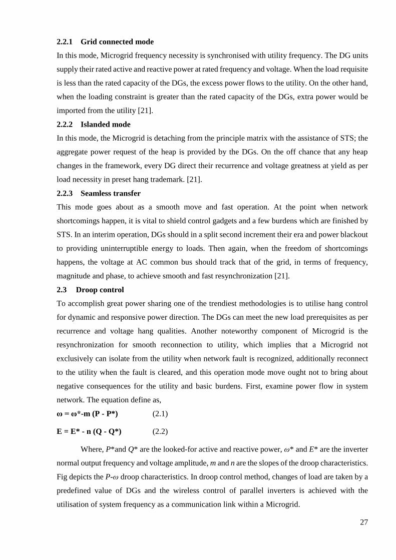
2.3 Droop control
To accomplish great power sharing one of the trendiest methodologies is to utilise hang control
for dynamic and responsive power direction. The DGs can meet the new load prerequisites as per
recurrence and voltage hang qualities. Another noteworthy component of Microgrid is the
resynchronization for smooth reconnection to utility, which implies that a Microgrid not
exclusively can isolate from the utility when network fault is recognized, additionally reconnect
to the utility when the fault is cleared, and this operation mode move ought not to bring about
negative consequences for the utility and basic burdens. First, examine power flow in system
network. The equation define as,
ω = ω*-m (P - P*) (2.1)
E = E* - n (Q - Q*) (2.2)
Where, P*and Q* are the looked-for active and reactive power, ω* and E* are the inverter
normal output frequency and voltage amplitude, m and n are the slopes of the droop characteristics.
Fig depicts the P-ω droop characteristics. In droop control method, changes of load are taken by a
predefined value of DGs and the wireless control of parallel inverters is achieved with the
utilisation of system frequency as a communication link within a Microgrid.

28
Overall Microgrid Network helps to protect the total breakdown or cascade tripping and to give
up the power in vital condition and keep the reliability of power line system in the grid. Also, it
helps to bring back in an emergency condition or faulty condition to protect those areas isolated
from the faulty area.
Figure 2.3 Active power and frequency drop characteristics 2.4 Power sharing for a Microgrid with MDG
Nowadays, the most important challenges considering noticeably growing load, less available fuel
sources, load shedding. But normally, there is a major part of losses by transmission and
distribution. These standards make the power system more complex. If power system is shifted on
renewable energy resources then, it is helpful to reduce the cost and attract customers also. The
most important thing is that DG is installed close to the customer so overall it is inexpensive as
compared to the central system [47].
Basically, a Microgrid performs in two operating states. If it is contacted to the power grid
at the point of common coupling then it is operating in grid-tied mode. In case if there exists any
breakdown occurs in Microgrid, it will switch over to island mode automatically which exhibits
that there is no possibility of power supply interruption to the end users. If it is standalone from
power grid then it is operating in island mode [47].
The Microgrid works on two power control modes like unit power output control (UPC) and
feeder flow control (FFC). These control modes gain its importance in the view of suitable power-
sharing along with DG units. UPC is planned for active power sharing with manifold DGs. In this
mode, the DG output power is maintained steady in accordance to the power reference while in
FFC mode; the DG power output is controlled to maintain the feeder flow steady [47].

29
3 Microgrid concept
A microgrid is a tiny network which is working autonomously and to provide a power for the small
region which contains different micro-sources, loads and some storage devices. There are two
different types of micro sources: DC sources and AC sources.
Figure 3.1 Basic block diagram of Microgrid [47]
In the power system static transfer switch automatically island the Microgrid from utility
due to disturbances, IEEE 1547 (power quality issues). If there is no longer present fault in the
system then Microgrid is reconnected and synchronises with frequency and voltage. Distributed
generations are small in size and power generation so it installed close to the customers [47].
Overall generation capacity range from kW to MW level.
Always generation at 11 kW or below.
Grid interconnection at distribution line side.
Inter-connected to a local grid, or fully off-grid system.
3.1 Frequency stabilisation in power sharing
In power system, the frequency is main parameters, which is maintained accurately in the range of
between 48.5 Hz to 50.5 Hz as per (IES). But now a day’s electricity regulatory revised a limit
from 49.05 to 50.02 Hz.
So that in the electrical power system, whenever the load side demand is suddenly
increased than the loading, is occurred on the generator and the frequency goes to drop down so it
will mandatory to maintain in between the range of frequency. If the load side demand is less and
the generation is more than the generator output is increased than required and the frequency goes
higher, in this condition important to maintain the frequency in the limits. Due to this problem in
frequency goes up and down anytime, the solution is to establish power sharing in between the
Microgrid and utility grid.
30
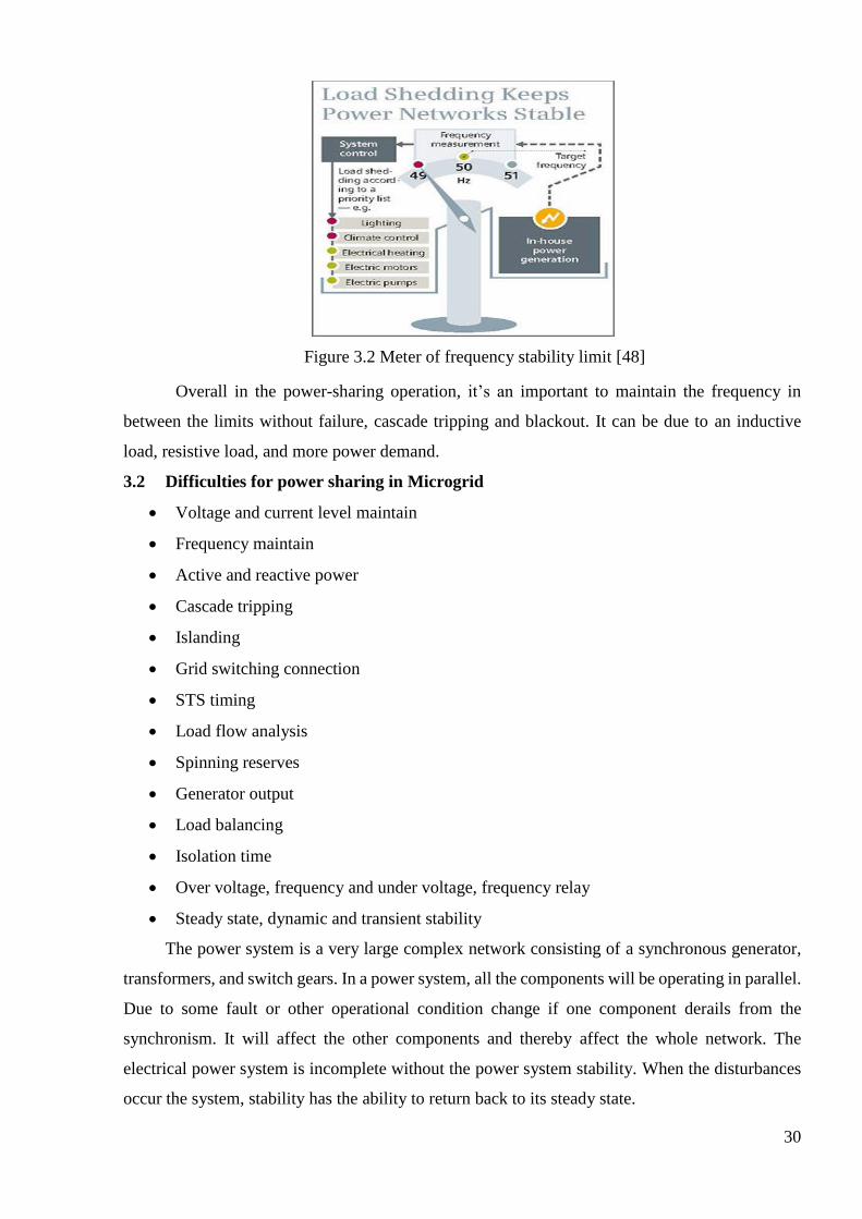
Figure 3.2 Meter of frequency stability limit [48]
Overall in the power-sharing operation, it’s an important to maintain the frequency in
between the limits without failure, cascade tripping and blackout. It can be due to an inductive
load, resistive load, and more power demand.
3.2 Difficulties for power sharing in Microgrid
Voltage and current level maintain
Frequency maintain
Active and reactive power
Cascade tripping
Islanding
Grid switching connection
STS timing
Load flow analysis
Spinning reserves
Generator output
Load balancing
Isolation time
Over voltage, frequency and under voltage, frequency relay
Steady state, dynamic and transient stability
The power system is a very large complex network consisting of a synchronous generator,
transformers, and switch gears. In a power system, all the components will be operating in parallel.
Due to some fault or other operational condition change if one component derails from the
synchronism. It will affect the other components and thereby affect the whole network. The
electrical power system is incomplete without the power system stability. When the disturbances
occur the system, stability has the ability to return back to its steady state.
31
3.3 How does Microgrid connect to main grid?
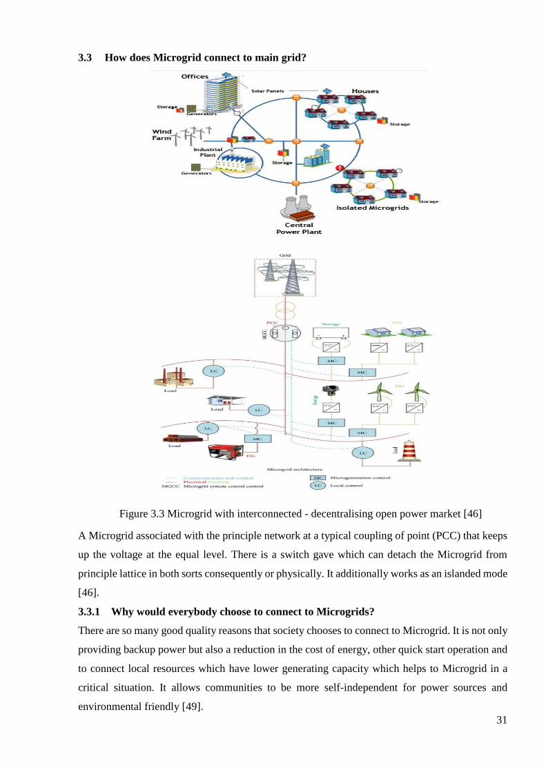
Figure 3.3 Microgrid with interconnected - decentralising open power market [46]
A Microgrid associated with the principle network at a typical coupling of point (PCC) that keeps
up the voltage at the equal level. There is a switch gave which can detach the Microgrid from
principle lattice in both sorts consequently or physically. It additionally works as an islanded mode
[46].
3.3.1 Why would everybody choose to connect to Microgrids?
There are so many good quality reasons that society chooses to connect to Microgrid. It is not only
providing backup power but also a reduction in the cost of energy, other quick start operation and
to connect local resources which have lower generating capacity which helps to Microgrid in a
critical situation. It allows communities to be more self-independent for power sources and
environmental friendly [49].

32
3.3.2 How much can a Microgrid power?
A Microgrid comes in open market with altered designs and sizes. As showing in the photos below
as an example of Microgrid can power a single facility like the small area in Santa Rita jail [49].
In today’s era when the technologies are more booming in Microgrid but not everywhere “Santa
Rita Jail” is the site of one of the best location for Microgrid model in the world.
Figure 3.4 Example of Microgrid at "SANTA RITA JAIL - CALIFORNIA" [49]
The jail has total approximately electrical Microgrid generation support are 1.5 MW of
photovoltaic, 1.0 MW molten carbonate fuel cell, back-up diesel generators can function grid
connected or islanded using a 2 MW and 4 MWh Lithium Ion battery as the only balancing
resource. The load demand is 3 MW more or less in peak time. So according to demand, the
electrical Microgrid sources are enough to maintain a peak load and system balancing. [49]
33
4 Energy demand side management
Problems
Some people are not agreed with demand-side management for the reason that it resulted in higher
utility costs for consumers and a lesser amount of amount of profit for utility.
For the demand side management system has a main goal whatever the price to consumers
that is true price of energy at that time. If the consumer’s usage not as much of in peak off hours
and high in peak time hours then automatically the fewer price charges attract to consumers to use
only that time energy than the goal is to be successfully achieved by DSM. One of the most
significant trouble in DSM is privacy that consumer is must be confirmed the personal information
and usage to the utility for demand side management [24] [28] [29].
4.1 Demand response
Demand response is a unique type of protocol that customer power consumption demand is
matched with a supply of utility. It is difficult to store power, so most utilities have by custom
coordinated to request and supply by quickening the creation rate of their energy plants, taking
producing units on or disconnected, periodically bringing in power from different utilities. There
are a few confinements what can be accomplished on the supply side in view of some of producing
units can set aside a long opportunity to come up in operation, some are extremely costly to work,
and another side request is higher than the limit so all power plants set up together in operation
[28]. Demand response is very difficult to adjust the demand for power instead of adjusting the
supply. If customers preferred lowest price for energy than utility postponed some task for
electrical power generation, so they shift their load on alternative sources like on-site diesel
generators [29].
Current scenario for current demand response schemes is applied for large, small and
residential customers, which all use their heavy loads in a particular time frame which is decided
the price for that time of energy and the same time their own on-site generation support to the grid
for demand management in balanced. So overall the cost is decreasing. In the event that the power
supply is tight than request reaction can essentially diminish the pinnacle cost and, all in all, power
value unpredictability [28].
Generally, the electrical transmission and distribution are related to peak demand, so if the
peak demand is less than overall the cost is going down for maintaining T & D. That’s why the
demand respond management to encourage the storage system which is on-site support in peak
time so overall price for energy goes down because of nearest location of power provider and
fewer losses [28].
34
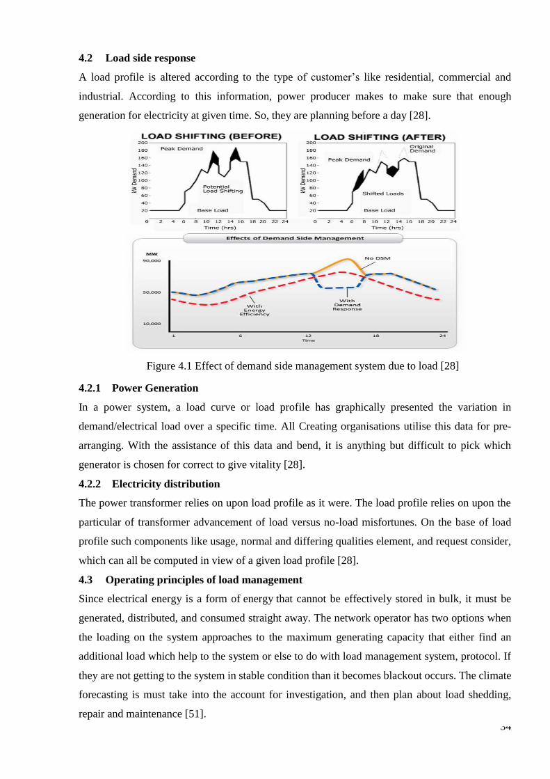
4.2 Load side response
A load profile is altered according to the type of customer’s like residential, commercial and
industrial. According to this information, power producer makes to make sure that enough
generation for electricity at given time. So, they are planning before a day [28].
Figure 4.1 Effect of demand side management system due to load [28]
4.2.1 Power Generation
In a power system, a load curve or load profile has graphically presented the variation in
demand/electrical load over a specific time. All Creating organisations utilise this data for pre-
arranging. With the assistance of this data and bend, it is anything but difficult to pick which
generator is chosen for correct to give vitality [28].
4.2.2 Electricity distribution
The power transformer relies on upon load profile as it were. The load profile relies on upon the
particular of transformer advancement of load versus no-load misfortunes. On the base of load
profile such components like usage, normal and differing qualities element, and request consider,
which can all be computed in view of a given load profile [28].
4.3 Operating principles of load management
Since electrical energy is a form of energy that cannot be effectively stored in bulk, it must be
generated, distributed, and consumed straight away. The network operator has two options when
the loading on the system approaches to the maximum generating capacity that either find an
additional load which help to the system or else to do with load management system, protocol. If
they are not getting to the system in stable condition than it becomes blackout occurs. The climate
forecasting is must take into the account for investigation, and then plan about load shedding,
repair and maintenance [51].

35
For the power plant, the capacity factor is most essential, so the utilisation of load
management system can help to plant to achieve the decisive goal. The output of power plant
compared to maximum output it could be produced that is called capacity factor. It is defined as
the ratio of average load to capacity or to peak load time limit. If the load factor is higher than it
benefits because due to that power plant should keep maintain efficiency less at low load factor
and if it is high than fixed costs are spread over more kWh of output which means larger total
output. The generator has to be adjusted when the power load factor is affected by non-availability
of fuel, maintenance, shut down, or reduced demand as consumption pattern fluctuate throughout
the day since grid energy storage is often prohibitively expensive [51].
Power costs are dependably crested in the mid-year. The cost to supply power changes
minute-by-moment. For the most part 90% buyers pay rates in light of the occasional cost of
power. In summer costs are constantly higher in light of the fact that request is lifted and era is not
adequate to give stack request so more expensive era is added to take care of the expanded demand.
Power costs change by sort of client [51]. Power costs are typically most noteworthy for private
and business shoppers since it costs more to disperse power to them. Modern buyers utilise
additional power and can get it at higher voltages, so it is further effective and less costly to supply
power to these clients when contrasted with the private or local load. The cost of electrical power
for modern clients is by and large near the discount cost of power due to a mass measure of
purchasing and substantial load [51].
4.4 Advantages of Deregulation
DISCOMS are divided into different companies for each individual function.
An open market for all – Privatisation.
Dropdown cost and customer’s service improvement.
Power generation and retail sales are competitive, monopoly franchise business.
Regulation
Regulation means that the Government has set down laws
and rules that put limits on and define how a particular
industry or company can operate.
Deregulation
Deregulation in power industry is a restructuring of the rules and economic incentives that government set up to control and drive electric power industry.
Figure 4.2 Difference between regulation and deregulation [51]

36
4.5 Power factor improvement and penalty factor
To measure of how effectively you're any electrical equipment converts electric power into useful
power output that is called power factor. In a technical point of view, it is the ratio of Active
Power (KW) to the Apparent Power (KVA) of an electrical installation [55].
KW is operational Power (Actual Power or Active Power or Real Power). It is the power that
actual power required by equipment for working only.
KVAR is Reactive Power. The magnetic equipment required to produce the magnetising flux
like transformer, motor and relays.
KVA is Apparent Power. It is the “Vectorial addition” of KVAR and KW.
The higher rate of percentage of KVAR, the lower your ratio of KW to KVA. So, the lower your
power factor. If your KVAR is lower, and ratio from KW to KVA is higher it means your KVAR
approaches zero, your power factor approaches 1.0.
Figure 4.3 Power factor triangle [55]
4.5.1 Why should improve the power factor?
Lower the Utility bill
In an electrical power system, all an inductive load requires reactive power; which reduces your
power factor. So, the requirement of more KVAR in the system reacts as required more KVA in
the system. Overall, extra power required from the utility. This means it is must amplify the
generation and transmission by the utility in the terms of handle this extra demand. In another side,
higher your power factor which using less KVAR. This results in less KW, which equates to
savings from the utility demand and saving your bill [55].
Increased overall system capacity and reduced losses
By adding capacitors KVAR generators to the system, the power factor is improved (<0.9) and the
KW capacity of the system is greater than before. Diminish I2R losses in cables [55].
Increased voltage level and cooling, more efficient motors (inductive load)
If power factor is not to be corrected than losses are more in the distribution system. So with
growing power losses more voltage drops. Extreme voltage drops can cause overheating and
unnecessary failure of motors and other inductive equipment which is heavy loaded. By raising
power factor, lessen the voltage drop in the feeder. If it is inductive load as a motor, motors will

37
run cooler and further efficient, with a fairly increase in capacity and starting torque. If it is 10%
terminal voltage drop have an effect on, [55]
It will shrink the Induction motor torque by approx. 19%,
Amplify full load current by approx. 11%,
Trim down overload capacity.
4.5.2 Reduces loading on transformers
Here introduced a typical transformer example, a 1,000 KVA transformer with an 80% power
factor provides 800 KW (600 KVAR) of power to the main bus.
(1000 KVA) 2 = (800 KW) 2 + (? KVAR) 2
KVAR = 600
By increasing the power factor to 90%, more KW can be supplied for the same amount of KVA.
(1000 KVA) 2 = (900 KW) 2 + (? KVAR) 2
KVAR = 436
The KW capacity of the system increased up to 900 KW and the utility supplies only 436 KVAR.
4.5.3 Power factor improvement methods
Static VAR Compensator(SVC)
Fixed Capacitors
Switched Capacitors
Synchronous Condensers
Static Synchronous Compensator(STATCOM)
Modulated power filter capacitor compensator
4.5.4 Disadvantages of lower power factor
Increases heating losses in the transformers and distribution equipment.
Overall Plant ageing effect goes down.
Voltage level unstable every stage.
Electrical power losses increase.
Higher cost for equipment up gradation.
Energy efficiency decreasing.
Power factor surcharges, increase electricity unit cost.
38
5 Availability based tariff - ABT
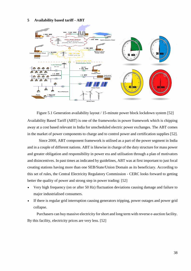
Figure 5.1 Generation availability layout / 15-minute power block lockdown system [52]
Availability Based Tariff (ABT) is one of the frameworks in power framework which is chipping
away at a cost based relevant in India for unscheduled electric power exchanges. The ABT comes
in the market of power components to charge and to control power and certification supplies [52].
Since 2000, ABT component framework is utilised as a part of the power segment in India
and in a couple of different nations. ABT is likewise in charge of the duty structure for mass power
and greater obligation and responsibility in power era and utilisation through a plan of motivators
and disincentives. In past times as indicated by guidelines, ABT was at first important to just focal
creating stations having more than one SEB/State/Union Domain as its beneficiary. According to
this set of rules, the Central Electricity Regulatory Commission - CERC looks forward to getting
better the quality of power and strong step in power trading: [52]
Very high frequency (on or after 50 Hz) fluctuation deviations causing damage and failure to
major industrialised consumers.
If there is regular grid interruption causing generators tripping, power outages and power grid
collapse.
Purchasers can buy massive electricity for short and long term with reverse e-auction facility.
By this facility, electricity prices are very less. [52]
39
5.1 Working operation of ABT
Each day of 24 hrs starting from 00.00 hours to be divided into 96-time blocks of 15 minutes
each. All generating station is to make press forward affirmation of its capacity for a generation
in terms of MWh delivery ex-bus for each time block of the next day. Even if there is a hydro
station also declare the daytime generation. While declaring the capability, the generator must
be ensuring that the capability during peak hours is not less than that during other hours. The
Scheduling is according with operating procedures [52].
After the beneficiaries give the conformation for generation schedules, then the RLDC is
prepared the generation and drawl schedules for each time block.
The schedule of actual generation shall be bulky on the ex-bus basis, whereas for beneficiaries,
scheduled drawls shall be quantified at their respective receiving points.
The transmission losses are considered and equally separated as per the drawl schedules and
that how much they can.
If any forced outage of a unit, or in the case of any transmission blocker, RLDC will revise the
schedules. The revised schedules will become effective from the 4th time block and counting,
but the revision is advised by 1st time only. It is also allowing for the generators and the
beneficiaries to revise schedules in a daytime only [52].
5.2 ABT feature
To maintain grid discipline and resolve grid disturbance issues.
Transparency of prices and increasing efficiency.
Requirements special meters with accurate time.
5.3 How ABT actively encourage trading?
A generating aptitude of a coal-fired power plant is 1000 MW. The plant has three beneficiaries’
states - A1, B1 and C1 with different load allocation 30%, 30% and 40 % correspondingly. If the
plant announces planned generating a capacity of 900 MW to the RLDC, the states then get 270,
270 and 360 MW electricity generations load correspondingly. Imagine, states A1 and B1 request
for entire share during the next 24 hrs and C1 output is 360 MW only during day time and 200
MW during the night, the generator has three options:
Totally shut down the entire station or
Find a buyer for the above off-peak surplus electricity. Existing buyers A1, B1 and C1 and the
new buyer. If the energy sale rate is higher than the fuel coast per kWh of the station, it would
be financial benefits for the station to enter such a deal. It would be helpful to reduce the shutting
down the entire station and improve station’s efficiency. If it’s more time allow, the Central
generating station may look around to find a party which would pay the highest rate and
maximise its profit.
40
As per the mutual agreement, the station accepts the schedule by RLDC instead of selling the
off-peak surplus power, but generates power to its full capability of 900 MW even during off-
peak hours. The result would be an over-supply of 160 MW as higher than schedule, for which
the station would get paid from the regional UI rate. So, at the end of the result, it would be a
sale to the regional pool, which gives benefits until the UI rate is higher than per kWh fuel cost
[52] [53].
Trading opportunity for state C
As per the requirement hold the power from the station.
Request to run on the full power of 360 MW from the central station for the entire 24-hour
period, find a buyer for the off-peak surplus power and to do agreement for power selling
bilaterally. Then after the sale rate per kWh is more than the energy charge rate of the central
station.
If drawing power as per requirement on full load next 24 hrs, the state would charge the present
UI rates. If the grid frequency is less than UI rates than the state shall profit from
underdrawing. In another case the frequency rises and the UI rates fall below the energy
charges, the state should reduce its requisition and stop underdrawing. The state has to make
sure that the UI charges during the off-peak hours remain higher than the energy charges of the
central generating station every time [52] [53].
5.4 Unscheduled Interchange (U.I)
Unscheduled Interchange is the under Drawl/Over drawl or under injection/over injection charges
against the scheduled power. Such as PAP is the power producer and INS is the customer to whom
it wants to sell power (say 200MW of power) [53].
As they don't have the direct transmission line, PAP will supply power to grid and grid will
supply the power to customer INS. Now, the catch is in power industry, PAP can’t supply exactly
200 MW and grid can’t supply exactly 200 MW to INS. There may be some variation, say PAP
supplied 205 MW. In this case, PAP will bill to INS for 200mw as per the price agreed with
customer and PAP will bill grid for 5 MW as per price set by the grid. This kind of billing which
attached with the grid is called UI billing. Similarly, the power supplied by PAP may be less say,
190mw. Again, in the same way, the grid also do the transaction with the customer INS. Point out
that, there are different factors that affect the billing that is frequency, time slots, capping charges
for over drawl/ under drawl, over/under injection, transmission losses, etc. They all must be
considered [51] [52] [53].
Open access always allows large users which have the capacity of at least 1MW or above to
buy cheaper electricity from the open market. This idea helpful to the customers to choose different
kind of power companies rather than only one [53].
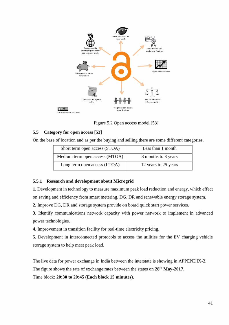
41
Figure 5.2 Open access model [53]
5.5 Category for open access [53]
On the base of location and as per the buying and selling there are some different categories.
Short term open access (STOA) Less than 1 month
Medium term open access (MTOA) 3 months to 3 years
Long term open access (LTOA) 12 years to 25 years
5.5.1 Research and development about Microgrid
1. Development in technology to measure maximum peak load reduction and energy, which effect
on saving and efficiency from smart metering, DG, DR and renewable energy storage system.
2. Improve DG, DR and storage system provide on board quick start power services.
3. Identify communications network capacity with power network to implement in advanced
power technologies.
4. Improvement in transition facility for real-time electricity pricing.
5. Development in interconnected protocols to access the utilities for the EV charging vehicle
storage system to help meet peak load.
The live data for power exchange in India between the interstate is showing in APPENDIX-2.
The figure shows the rate of exchange rates between the states on 28th May-2017.
Time block: 20:30 to 20:45 (Each block 15 minutes).
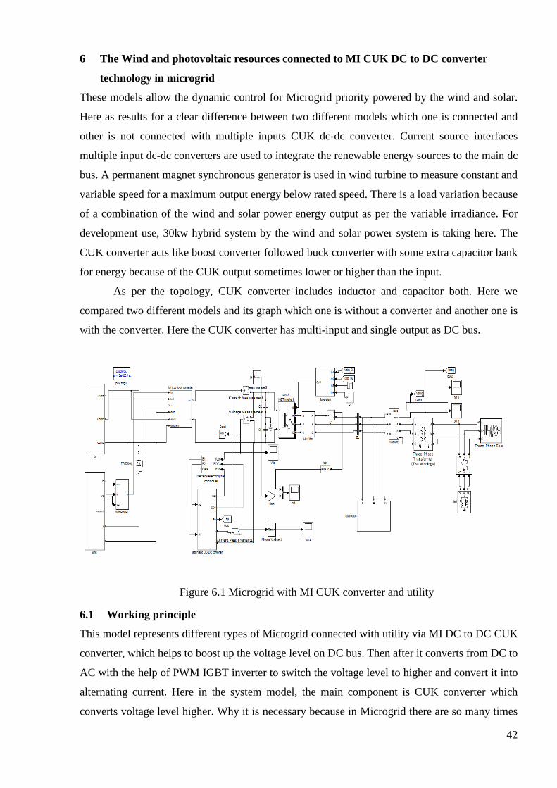
42
6 The Wind and photovoltaic resources connected to MI CUK DC to DC converter
technology in microgrid
These models allow the dynamic control for Microgrid priority powered by the wind and solar.
Here as results for a clear difference between two different models which one is connected and
other is not connected with multiple inputs CUK dc-dc converter. Current source interfaces
multiple input dc-dc converters are used to integrate the renewable energy sources to the main dc
bus. A permanent magnet synchronous generator is used in wind turbine to measure constant and
variable speed for a maximum output energy below rated speed. There is a load variation because
of a combination of the wind and solar power energy output as per the variable irradiance. For
development use, 30kw hybrid system by the wind and solar power system is taking here. The
CUK converter acts like boost converter followed buck converter with some extra capacitor bank
for energy because of the CUK output sometimes lower or higher than the input.
As per the topology, CUK converter includes inductor and capacitor both. Here we
compared two different models and its graph which one is without a converter and another one is
with the converter. Here the CUK converter has multi-input and single output as DC bus.
Figure 6.1 Microgrid with MI CUK converter and utility
6.1 Working principle
This model represents different types of Microgrid connected with utility via MI DC to DC CUK
converter, which helps to boost up the voltage level on DC bus. Then after it converts from DC to
AC with the help of PWM IGBT inverter to switch the voltage level to higher and convert it into
alternating current. Here in the system model, the main component is CUK converter which
converts voltage level higher. Why it is necessary because in Microgrid there are so many times

43
frequency deviation and ramp rates in PV and wind so whenever the renewable energy resources
are available at stable irradiance than CUK converter boost the voltage which helps to reduce the
loading and usage of the utility grid. If the irradiance varying than it should be affected by overall
system frequency which is going up and down due to ramp rates.
There is a battery storage unit which helps to maintain reactive power in the system when
the supply voltage from Microgrid of each different source goes down than specific limits. Here
as per the model, there is a local load and some 3 phase other loads are there. When the Microgrid
like PV or wind generate the electrical power with the help of MPPT to reach a point of maximum
output then it passes through the CUK converter which boosts up the voltage and then by inverter
it converts into AC. So, overall as per the load's requirement those amount of power which is
generated by renewable energy Microgrid which runs the loads and if there is not enough power
than the remaining amount of power taken by the utility grid. There is also battery storage unit in
Microgrid which helps to maintain stability in the network when required active power and more
voltage. The working operation is explained by the graph.
As in the voltage output graph of wind and PV before converter and after converter there
is a drastic different. In the voltage graph of wind the highest peak value is 23.4 V and then slightly
decreasing and in the PV it’s changing because of different irradiance but in the second graph after
converter which boosts up the voltage up to 175 V of the system which is Vdc on bus voltage.
Graph 6.1 Voltage comparison (without-with)
As in the current also there is a little bit different point of view than voltage. The PV current
is increasing and decreasing which is not so stable. Before converter output current from the wind
is very high but after converter, it is comparing with filter and on main bus current. The graph
shows that after converter output current is gradually boosted up to limits as per the system but
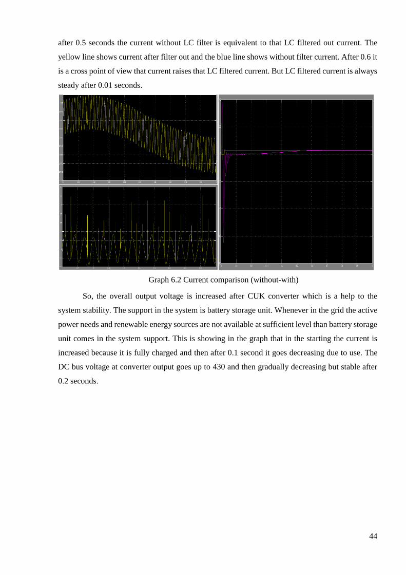
44
after 0.5 seconds the current without LC filter is equivalent to that LC filtered out current. The
yellow line shows current after filter out and the blue line shows without filter current. After 0.6 it
is a cross point of view that current raises that LC filtered current. But LC filtered current is always
steady after 0.01 seconds.
Graph 6.2 Current comparison (without-with)
So, the overall output voltage is increased after CUK converter which is a help to the
system stability. The support in the system is battery storage unit. Whenever in the grid the active
power needs and renewable energy sources are not available at sufficient level than battery storage
unit comes in the system support. This is showing in the graph that in the starting the current is
increased because it is fully charged and then after 0.1 second it goes decreasing due to use. The
DC bus voltage at converter output goes up to 430 and then gradually decreasing but stable after
0.2 seconds.
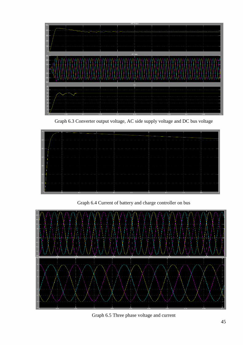
45
Graph 6.3 Converter output voltage, AC side supply voltage and DC bus voltage
Graph 6.4 Current of battery and charge controller on bus
Graph 6.5 Three phase voltage and current

46
Graph 6.6 Active and reactive power
As for showing in above graph the reactive power control support to active power at 0.005
seconds. So, in the system when the utility grid usage goes down than a still generation is more or
if the demand is more than generation reactive power is control to active power and the results are
achieved here. It is also affected by Microgrid of renewable energy resources because those are
different power injection in the grid. PV and the wind are generating active and reactive power
respectively so, it is affected by the utility grid network if it is not in balance.
Numerous same frameworks in control components yet two of them as of now exists. For
instance, network associated PMSG WTs required stable DC connect voltage and to guarantee that
a settlement is kept up by dynamic power stream. Regularly, dynamic and responsive power
control from both sides is balanced out DC voltage. At the point when, the DC voltage higher than
the reference esteem, the converter naturally infuses dynamic power in the matrix to diminish the
DC connect voltage. If there is a fault occurs in the grid or restoration of voltage then, reactive
power support control is on higher preferences as compared to active power balance. When the
voltage fluctuation is more, converter control allows reducing active power generated by the
system.
Another side in PV for DC, electrical power is the result of voltage and current. In AC side
the power and heading of current and voltage change on general premise. In the private grid, both
current and voltage have a sinusoidal waveform with frequency 50or 60 Hz and both are in phase
so; the output is average positive which is pure active power. In the event that voltage and current
are moved against each other then the yield is substituting positive and negative and the outcome
is immaculate receptive power. Most probably when the voltage is zero, current reaches maximum
point and vice versa. The result is pure reactive power, the positive and negative sign completely
neutralise to each other.
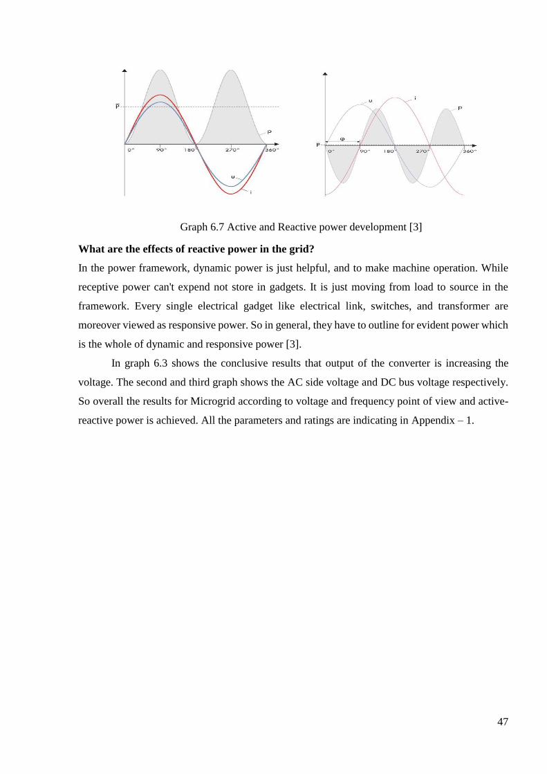
47
Graph 6.7 Active and Reactive power development [3] What are the effects of reactive power in the grid?
In the power framework, dynamic power is just helpful, and to make machine operation. While
receptive power can't expend not store in gadgets. It is just moving from load to source in the
framework. Every single electrical gadget like electrical link, switches, and transformer are
moreover viewed as responsive power. So in general, they have to outline for evident power which
is the whole of dynamic and responsive power [3].
In graph 6.3 shows the conclusive results that output of the converter is increasing the
voltage. The second and third graph shows the AC side voltage and DC bus voltage respectively.
So overall the results for Microgrid according to voltage and frequency point of view and active-
reactive power is achieved. All the parameters and ratings are indicating in Appendix – 1.
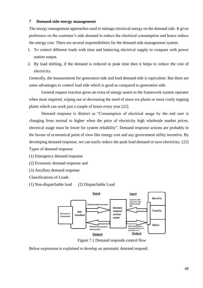
48
7 Demand-side energy management
The energy management approaches used to ménage electrical energy on the demand side. It gives
preference on the customer’s side demand to reduce the electrical consumption and hence reduce
the energy cost. There are several responsibilities for the demand side management system.
1. To control different loads with time and balancing electrical supply to compare with power
station output.
2. By load shifting, if the demand is reduced in peak time then it helps to reduce the cost of
electricity.
Generally, the measurement for generation side and load demand side is equivalent. But there are
some advantages to control load side which is good as compared to generation side.
General request reaction gives an extra of energy assets to the framework system operator
when most required, wiping out or decreasing the need of more era plants or most costly topping
plants which can work just a couple of hours every year [22].
Demand response is distinct as “Consumption of electrical usage by the end user is
changing from normal to higher when the price of electricity high wholesale market prices,
electrical usage must be lower for system reliability”. Demand response actions are probably in
the favour of economical point of view like energy cost and any government utility incentive. By
developing demand response, we can easily reduce the peak load demand or save electricity. [22]
Types of demand response
(1) Emergency demand response
(2) Economic demand response and
(3) Ancillary demand response
Classifications of Loads
(1) Non-dispatchable load (2) Dispatchable Load
Figure 7.1 Demand responds control flow
Below expression is explained to develop an automatic demand respond.
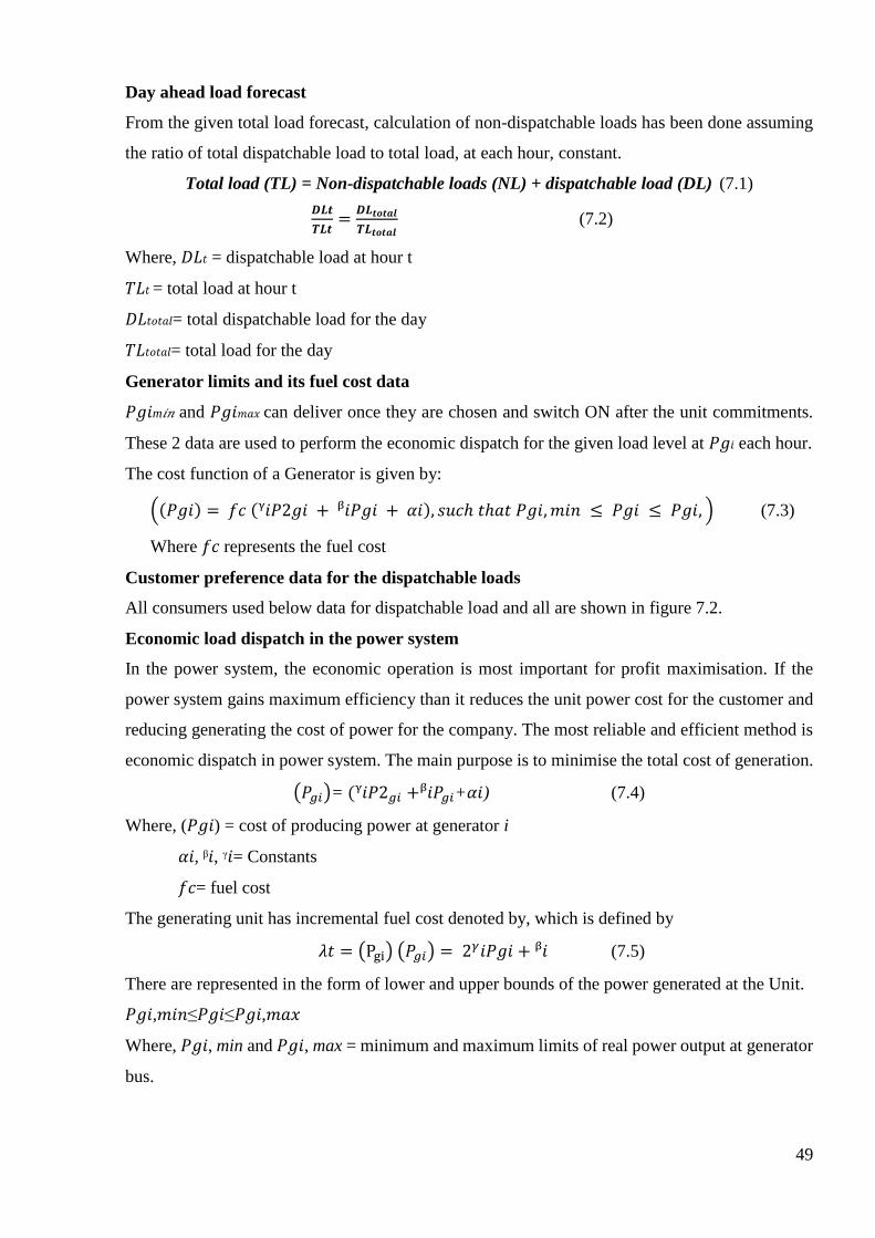
49
Day ahead load forecast
From the given total load forecast, calculation of non-dispatchable loads has been done assuming
the ratio of total dispatchable load to total load, at each hour, constant.
Total load (TL) = Non-dispatchable loads (NL) + dispatchable load (DL) (7.1)
𝑫𝑳𝒕
𝑻𝑳𝒕=
𝑫𝑳𝒕𝒐𝒕𝒂𝒍
𝑻𝑳𝒕𝒐𝒕𝒂𝒍
(7.2)
Where, 𝐷𝐿𝑡 = dispatchable load at hour t
𝑇𝐿𝑡 = total load at hour t
𝐷𝐿𝑡𝑜𝑡𝑎𝑙= total dispatchable load for the day
𝑇𝐿𝑡𝑜𝑡𝑎𝑙= total load for the day
Generator limits and its fuel cost data
𝑃𝑔𝑖m𝑖𝑛 and 𝑃𝑔𝑖𝑚𝑎𝑥 can deliver once they are chosen and switch ON after the unit commitments.
These 2 data are used to perform the economic dispatch for the given load level at 𝑃𝑔𝑖 each hour.
The cost function of a Generator is given by:
((𝑃𝑔𝑖) = 𝑓𝑐 (ᵞ𝑖𝑃2𝑔𝑖 + ᵝ𝑖𝑃𝑔𝑖 + 𝛼𝑖), 𝑠𝑢𝑐ℎ 𝑡ℎ𝑎𝑡 𝑃𝑔𝑖, 𝑚𝑖𝑛 ≤ 𝑃𝑔𝑖 ≤ 𝑃𝑔𝑖, ) (7.3)
Where 𝑓𝑐 represents the fuel cost
Customer preference data for the dispatchable loads
All consumers used below data for dispatchable load and all are shown in figure 7.2.
Economic load dispatch in the power system
In the power system, the economic operation is most important for profit maximisation. If the
power system gains maximum efficiency than it reduces the unit power cost for the customer and
reducing generating the cost of power for the company. The most reliable and efficient method is
economic dispatch in power system. The main purpose is to minimise the total cost of generation.
(𝑃𝑔𝑖)= (ᵞ𝑖𝑃2𝑔𝑖 +ᵝ𝑖𝑃𝑔𝑖+𝛼𝑖) (7.4)
Where, (𝑃𝑔𝑖) = cost of producing power at generator i
𝛼𝑖, ᵝ𝑖, ᵞ𝑖= Constants
𝑓𝑐= fuel cost
The generating unit has incremental fuel cost denoted by, which is defined by
𝜆𝑡 = (Pgi) (𝑃𝑔𝑖) = 2𝛾𝑖𝑃𝑔𝑖 + ᵝ𝑖 (7.5)
There are represented in the form of lower and upper bounds of the power generated at the Unit.
𝑃𝑔𝑖,𝑚𝑖𝑛≤𝑃𝑔𝑖≤𝑃𝑔𝑖,𝑚𝑎𝑥
Where, 𝑃𝑔𝑖, min and 𝑃𝑔𝑖, max = minimum and maximum limits of real power output at generator
bus.
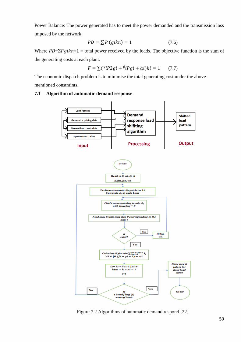
50
Power Balance: The power generated has to meet the power demanded and the transmission loss
imposed by the network.
𝑃𝐷 = ∑ 𝑃 (𝑔𝑖𝑘𝑛) = 1 (7.6)
Where 𝑃𝐷=Σ𝑃𝑔𝑖𝑘𝑛=1 = total power received by the loads. The objective function is the sum of
the generating costs at each plant.
𝐹 = ∑( ᵞ𝑖𝑃2𝑔𝑖 + ᵝ𝑖𝑃𝑔𝑖 + 𝛼𝑖)𝑘𝑖 = 1 (7.7)
The economic dispatch problem is to minimise the total generating cost under the above-
mentioned constraints.
7.1 Algorithm of automatic demand response
Figure 7.2 Algorithms of automatic demand respond [22]
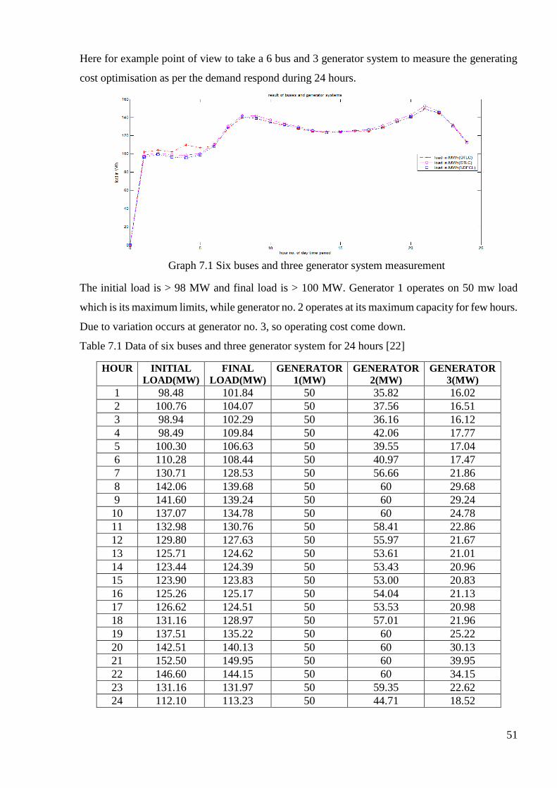
51
Here for example point of view to take a 6 bus and 3 generator system to measure the generating
cost optimisation as per the demand respond during 24 hours.
Graph 7.1 Six buses and three generator system measurement
The initial load is > 98 MW and final load is > 100 MW. Generator 1 operates on 50 mw load
which is its maximum limits, while generator no. 2 operates at its maximum capacity for few hours.
Due to variation occurs at generator no. 3, so operating cost come down.
Table 7.1 Data of six buses and three generator system for 24 hours [22]
HOUR INITIAL
LOAD(MW)
FINAL
LOAD(MW)
GENERATOR
1(MW)
GENERATOR
2(MW)
GENERATOR
3(MW)
1 98.48 101.84 50 35.82 16.02
2 100.76 104.07 50 37.56 16.51
3 98.94 102.29 50 36.16 16.12
4 98.49 109.84 50 42.06 17.77
5 100.30 106.63 50 39.55 17.04
6 110.28 108.44 50 40.97 17.47
7 130.71 128.53 50 56.66 21.86
8 142.06 139.68 50 60 29.68
9 141.60 139.24 50 60 29.24
10 137.07 134.78 50 60 24.78
11 132.98 130.76 50 58.41 22.86
12 129.80 127.63 50 55.97 21.67
13 125.71 124.62 50 53.61 21.01
14 123.44 124.39 50 53.43 20.96
15 123.90 123.83 50 53.00 20.83
16 125.26 125.17 50 54.04 21.13
17 126.62 124.51 50 53.53 20.98
18 131.16 128.97 50 57.01 21.96
19 137.51 135.22 50 60 25.22
20 142.51 140.13 50 60 30.13
21 152.50 149.95 50 60 39.95
22 146.60 144.15 50 60 34.15
23 131.16 131.97 50 59.35 22.62
24 112.10 113.23 50 44.71 18.52

52
Table 7.2 Allotted start hour for various loads [22]
Load
number
Load value,
𝒍𝒊 (*10 W)
Uptime 𝒖𝒊 Downtime
𝒇𝒊 Duration
𝒓𝒊 (hours)
Allotted
star
hours
1 5 1 10 4 1
2 8 2 12 2 4
3 3 10 24 2 23
4 2 12 20 3 14
5 1 8 16 2 13
Table 7.3 Old and new load curve data for six buses. [22]
Maximum
load(MW)
Minimum
Load(MW)
Hour for
Maximum
load
Hour for
Minimum
load
Average
Load(MW)
Std
devn.
Load
Factor
Six bus
(new)
149.95 101.86 21 1 125.00 13.88 0.83
Six bus
(old)
152.50 98.5 21 4 125.00 16.5 0.82
By using automatic demand response, we fit the load curve by shift the demand with the
help of load shifting algorithm. We make the load curve more stable than the old one, as well as
we improve the efficiency of the system and improve the load factor. Hence, we can manage the
power by using automatic demand response.
Future work
By using demand response, we can manage the load or we can shift the load and make load curve
stable. To improve the efficiency of the system this can be used in smart meters’ controller.
7.2 Price based demand response
Characterization of demand response programme
Figure 7.3 Types of demand response [13]
7.2.1 Methodology and proposed algorithms
Here there are two different scenarios; in the first case time of use (TOU tariff) is applied
during off-peak periods. The rate of TOU tariff will be lower than peak period. Indirect control

53
customers encouraged to shift their energy use to off-peak times keeping a good level of comfort
but with a little change in life. It means to give a control of electricity to customers themselves.
In the second case the flat tariff is applied where the customers pay the same rate of electricity
consumed and through direct control as home and big buildings energy management process of
shedding the loads as per the priority level and adjust the maximum power threshold at high level
without any compromising the people’s comfort and flow chart which showing in algorithm. [13]
Figure 7.4 Priority control flow chart [13]
Here is a model from MATLAB/SIMULINK representing how the demand side
management control management and for simulation purpose time 1 second as 1 hour in the real
life. This model is not a real model to run it is a reference model just for showing that how to
connect different sources to loads with the algorithm.
7.3 Simulation results
The reference model of MATLAB/SIMULINK shows that there is a significant decrease in energy
and cost in the first scenario while in the second scenario the decrease in energy and cost was
lower than in the first scenario as shown in the graph 7.2 [13]
Figure 7.5 Simulation diagram and appliance priority table [13]

54
Graph 7.2 Results of load profile [13]
7.4 Overall results
The demand responds programs gives benefits to the customers and try to change their use of
appliances and routine lifestyle and comfort changes in operating procedures. Some of the changes
are allowed only if the customers have a stake in the process either through financial compensation
by electricity bill reduction and incentive payments as a cost of being flexible in terms of accepting
a wider comfort zone or through improved reliability of power supply.
In our case study, it was obvious that the second scenario didn’t save a remarkable
percentage of either the energy this is because the very high level of comfort that was given as the
threshold of the maximum power was set to 10.1 KW while in the first scenario there were a wide
area of flexibility by changing the lifestyle but keeping a good level of comfort leading to
magnificent both energy saving.
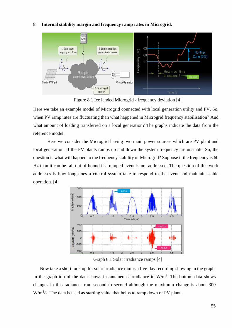
55
8 Internal stability margin and frequency ramp rates in Microgrid.
Figure 8.1 Ice landed Microgrid - frequency deviation [4]
Here we take an example model of Microgrid connected with local generation utility and PV. So,
when PV ramp rates are fluctuating than what happened in Microgrid frequency stabilisation? And
what amount of loading transferred on a local generation? The graphs indicate the data from the
reference model.
Here we consider the Microgrid having two main power sources which are PV plant and
local generation. If the PV plants ramps up and down the system frequency are unstable. So, the
question is what will happen to the frequency stability of Microgrid? Suppose if the frequency is 60
Hz than it can be fall out of bound if a ramped event is not addressed. The question of this work
addresses is how long does a control system take to respond to the event and maintain stable
operation. [4]
Graph 8.1 Solar irradiance ramps [4]
Now take a short look up for solar irradiance ramps a five-day recording showing in the graph.
In the graph top of the data shows instantaneous irradiance in W/m2. The bottom data shows
changes in this radiance from second to second although the maximum change is about 300
W/m2/s. The data is used as starting value that helps to ramp down of PV plant.

56
Graph 8.2 Ramp rates frequency decay and magnitude [4]
This chart shows the impact of ramp rates on frequency decay. The first chart shows ramp
rates varying from -10 MWs to +10 MWs. Another chart shows hours the frequency is expected to
change if there is no action control taken. So, the ramp rate magnitude has an important effect on
how much time there is to respond to the event.
Graph 8.3 Frequency ramp rates and system inertia [4]
Another important factor is Microgrid inertia constant because frequency varies inversely
proportional to the inertia constant. If suppose here the system capacity of 10 MVA. The deviation
value must be defined by some bounded values and it can be adjusted from control setting.
|∆𝒇𝒑𝒖| < 0.05
5% of nominal (+/-3 Hz); Frequency deviation in (Pu-Hz)
Here the chart shows pictorial representation that if you have 3 KW hours if stored energy
in your spinning generation under a ramp event of 2 MW per second than you would have
approximately between 0.8 to 1 second time to respond. If you have 4 KW storage systems than
time is little increasing up to 1.2 seconds. The amount of energy stored in the rotor is directly
proportional to the system inertia constant and system power capacity.
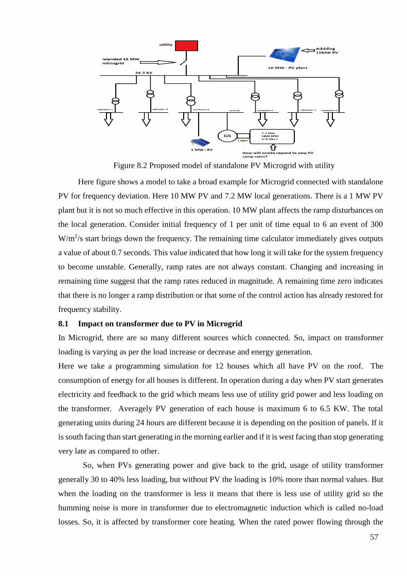
57
Figure 8.2 Proposed model of standalone PV Microgrid with utility
Here figure shows a model to take a broad example for Microgrid connected with standalone
PV for frequency deviation. Here 10 MW PV and 7.2 MW local generations. There is a 1 MW PV
plant but it is not so much effective in this operation. 10 MW plant affects the ramp disturbances on
the local generation. Consider initial frequency of 1 per unit of time equal to 6 an event of 300
W/m2/s start brings down the frequency. The remaining time calculator immediately gives outputs
a value of about 0.7 seconds. This value indicated that how long it will take for the system frequency
to become unstable. Generally, ramp rates are not always constant. Changing and increasing in
remaining time suggest that the ramp rates reduced in magnitude. A remaining time zero indicates
that there is no longer a ramp distribution or that some of the control action has already restored for
frequency stability.
8.1 Impact on transformer due to PV in Microgrid
In Microgrid, there are so many different sources which connected. So, impact on transformer
loading is varying as per the load increase or decrease and energy generation.
Here we take a programming simulation for 12 houses which all have PV on the roof. The
consumption of energy for all houses is different. In operation during a day when PV start generates
electricity and feedback to the grid which means less use of utility grid power and less loading on
the transformer. Averagely PV generation of each house is maximum 6 to 6.5 KW. The total
generating units during 24 hours are different because it is depending on the position of panels. If it
is south facing than start generating in the morning earlier and if it is west facing than stop generating
very late as compared to other.
So, when PVs generating power and give back to the grid, usage of utility transformer
generally 30 to 40% less loading, but without PV the loading is 10% more than normal values. But
when the loading on the transformer is less it means that there is less use of utility grid so the
humming noise is more in transformer due to electromagnetic induction which is called no-load
losses. So, it is affected by transformer core heating. When the rated power flowing through the
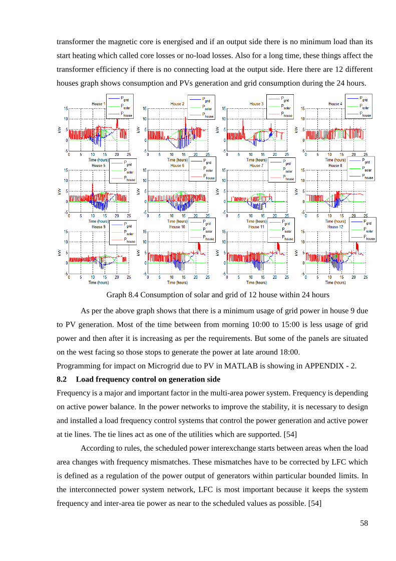
58
transformer the magnetic core is energised and if an output side there is no minimum load than its
start heating which called core losses or no-load losses. Also for a long time, these things affect the
transformer efficiency if there is no connecting load at the output side. Here there are 12 different
houses graph shows consumption and PVs generation and grid consumption during the 24 hours.
Graph 8.4 Consumption of solar and grid of 12 house within 24 hours
As per the above graph shows that there is a minimum usage of grid power in house 9 due
to PV generation. Most of the time between from morning 10:00 to 15:00 is less usage of grid
power and then after it is increasing as per the requirements. But some of the panels are situated
on the west facing so those stops to generate the power at late around 18:00.
Programming for impact on Microgrid due to PV in MATLAB is showing in APPENDIX - 2.
8.2 Load frequency control on generation side
Frequency is a major and important factor in the multi-area power system. Frequency is depending
on active power balance. In the power networks to improve the stability, it is necessary to design
and installed a load frequency control systems that control the power generation and active power
at tie lines. The tie lines act as one of the utilities which are supported. [54]
According to rules, the scheduled power interexchange starts between areas when the load
area changes with frequency mismatches. These mismatches have to be corrected by LFC which
is defined as a regulation of the power output of generators within particular bounded limits. In
the interconnected power system network, LFC is most important because it keeps the system
frequency and inter-area tie power as near to the scheduled values as possible. [54]

59
Input mechanical power to the generator is used to control the frequency of the output as electrical
power and to maintain the power exchange between two points as scheduled. If the design of LFC
is perfect than it matched with a change of load and system disturbances to maintaining both
voltage and frequency within sustainable limits.
Electrical power is generated by mechanical energy converting into electrical energy. The
rotor weight which contains turbine and generator units stores kinetic energy due to the rotation.
Due to this stored kinetic energy, there is a sudden impact on load increase. For mathematical
expression, mechanical torque input denoted by Tm and the output electrical torque denoted by
Te. When the difference between two elements is zero, rotational losses are negligible. For here
the accelerating torque is zero. [54]
𝑻𝒂 = 𝑻𝒎 − 𝑻𝒆
Whenever the electrical power demand rises, suddenly at same time electrical torque rises.
Because of the feedback control loop, Tm is remaining at constant and due to rotor mass
accelerating torque is negative. The rotor releases kinetic energy and supply to boost up load.
During that time the system frequency goes down. When Tm < Te the frequency goes drop down
and rises when Tm > Te. The relation of steady state power is showing in fig.9.7. In this figure,
the slope of the ΔPref line is negative and is given by
−𝑹 = ∆𝒇/∆𝑷𝒎 (R = regulating constant)
Figure 8.3 Load frequency control mechanism [54]
The LFC method is performed by an ISO based parameter which is defined by generating
units. It included utility generators and independent power producers. Under load frequency
control, independent power producers may not participate in the LFC control. Here figure shows
SIMULINK model of the isolated uncontrolled power system.

60
Graph 8.5 Comparison between without LFC and with LFC
As per the graph in first there is no LFC control so the frequency is not in the stable region
as it is a starting point. In the second graph, there is LFC control so as per the overall system output
the feedback control loop gives feedback signal to input block so the frequency is coming back in
original steady state value after 10 or 12 seconds.
From the graph comparison both responses equivalent with each other, also the steady-
state frequency deviation ∆f (steady state) is zero and frequency return to its steady value in
approximately 12 seconds. (After 10 second). This result displayed stable frequency. Tie line
power, frequency deviations and dual mode controller are effectively controlled if the rated
parameters are perfect. Due to disturbances in the power system, the frequency is deviated.

61
9 Conclusions
The investigation of the model of Microgrid linked utility at optimal power sharing and the results
are achieved here and explain in the earlier chapters. Traditional approaches are to integrating
distributed energy resources into distribution network and minimising the consequence for
protection and involve SPIDER network Microgrid to operate grid connected and islanded mode.
The performance of the system is cost effective which is achieved by this project examination.
1. After experimented from MATLAB/SIMULINK model for the first task, it is concluded that
if the strong design and perfect algorithm architecture for DC-DC CUK converter are done
then the control for optimal power sharing is very easy. From the results, it is clear effect
shows that without multi-input CUK converter output is far less than proposed a model. All
the parameters for the grid like voltage, current, active and reactive power is controlled and
stable. The priority of active and reactive power control is done by first from renewable energy
resources and then after utility grid. The result is achieved here as an efficient and optimal
level power sharing even if the load is varying.
2. DC-DC CUK converter interfaces the renewable energy resource, optimal power sharing is
achieved by an auxiliary inverter and droop control P, Q characteristics with lower frequency
deviation.
3. For the demand side, management control is done by the special design algorithm and price-
based system. Recently it is on development stage and little difficult for the consumer but the
result is achieved here from the reference 6 buses and 3 generator system and it should be
effective and easy too.
4. In the final task, the frequency margin is achieved in minimum time at 0.12 second as per the
LFC connected system graph. If the fluctuation is more and out of limits, then the control
theory feedback protection system helps to improve the frequency quickly. Because the time
is important for stability margin to come back system in steady state condition. The result is
showing here in the graph when suddenly; loading increased the deviation of frequency is
controlled by LFC and it comes back in steady state condition after 0.12 seconds.
5. System response and power quality distribution are achieved by LC filter and load balancing
technique and reactive power compensation during real power supply.
Overall the conclusion for the whole project is to connect various renewable energy resources with
utility grid and to make a system stress free. Power sharing is a useful method to balance the system
network with Microgrid. Forecasting equation is modified and improves more reliable operation.
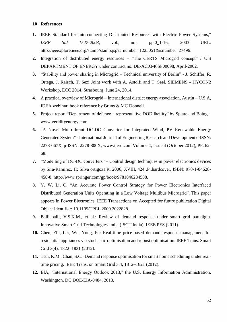
62
10 References
1. IEEE Standard for Interconnecting Distributed Resources with Electric Power Systems,"
IEEE Std 1547-2003, vol., no., pp.0_1-16, 2003 URL:
http://ieeexplore.ieee.org/stamp/stamp.jsp?arnumber=1225051&isnumber=27496.
2. Integration of distributed energy resources – “The CERTS Microgrid concept” / U.S
DEPARTMENT OF ENERGY under contract no. DE-AC03-I6SF00098, April-2002.
3. “Stability and power sharing in Microgrid – Technical university of Berlin” - J. Schiffer, R.
Ortega, J. Raisch, T. Sezi Joint work with A. Astolfi and T. Seel, SIEMENS - HYCON2
Workshop, ECC 2014, Strasbourg, June 24, 2014.
4. A practical overview of Microgrid – International district energy association, Austin – U.S.A,
IDEA webinar, book reference by Bruns & MC Donnell.
5. Project report “Department of defence – representative DOD facility” by Spiare and Boing –
www.veridityenergy.com
6. “A Novel Multi Input DC-DC Converter for Integrated Wind, PV Renewable Energy
Generated System” - International Journal of Engineering Research and Development e-ISSN:
2278-067X, p-ISSN: 2278-800X, www.ijerd.com Volume 4, Issue 4 (October 2012), PP. 62-
68.
7. “Modelling of DC-DC converters” – Control design techniques in power electronics devices
by Sira-Ramirez. H: Silva ortigoza.R. 2006, XVIII, 424 .P.,hardcover, ISBN: 978-1-84628-
458-8. http://www.springer.com/gp/book/9781846284588.
8. Y. W. Li, C. “An Accurate Power Control Strategy for Power Electronics Interfaced
Distributed Generation Units Operating in a Low Voltage Multibus Microgrid”. This paper
appears in Power Electronics, IEEE Transactions on Accepted for future publication Digital
Object Identifier: 10.1109/TPEL.2009.2022828.
9. Balijepalli, V.S.K.M., et al.: Review of demand response under smart grid paradigm.
Innovative Smart Grid Technologies-India (ISGT India), IEEE PES (2011).
10. Chen, Zhi, Lei, Wu, Yong, Fu: Real-time price-based demand response management for
residential appliances via stochastic optimisation and robust optimisation. IEEE Trans. Smart
Grid 3(4), 1822–1831 (2012).
11. Tsui, K.M., Chan, S.C.: Demand response optimisation for smart home scheduling under real-
time pricing. IEEE Trans. on Smart Grid 3.4, 1812–1821 (2012).
12. EIA, "International Energy Outlook 2013," the U.S. Energy Information Administration,
Washington, DC DOE/EIA-0484, 2013.

63
13. Power Sharing Method for a Grid-connected Microgrid with Multiple Distributed Generators
- Journal of Electrical Engineering & Technology Vol. 7, No. 4, pp. 459~467, 2012
http://dx.doi.org/10.5370/JEET.2012.7.4.459459
14. A. Rifat BOYNUEGRI, B. YAGCITEKIN, M. BAYSAL, A. KARAKAS and M.
UZUNOGLU, "Energy Management Algorithm for Smart Home with Renewable Energy
Sources," in 4th International Conference on Power Engineering, Energy and Electrical
Drives, Istanbul, Turkey, 13-17 May 2013.
15. Mahnoosh Alizadeh, Zhifang Wang and Anna Scaglione, "Demand Side Management Trends
in the Power Grid," in 4th IEEE International Workshop on Computational Advances in Multi-
Sensor Adaptive Processing (CAMSAP), 2011.
16. J. Torriti, M. G. Hassan and M. Leach, “Demand Response Experience in Europe: Policies,
Programmes and Implementation,” Energy, Vol. 35, No. 4, 2009, pp. 1575-1583. doi:
10.1016/j.energy.2009.05.021.
17. M. H. Albadi and E. F. El-Saadany, "A summary of demand response in electricity markets,"
Electric Power Systems Research, vol. 78, pp. 1989-1996, 2008.
18. SA, "AS5711-2013: Smart grid vocabulary," ed. Australia, 2013.
19. N. D. Hatziargyriou, “Special issue on Microgrids and energy management,” European
Transactions on Electrical Power, vol.21, no. 2, pp. 1139–1141, 2011.
20. F. A. Mohamed andH. N. Koivo, “System modelling and online optimal management of
Microgrid with battery storage,” in Proceedings of the International Conference on
Renewable Energies and Power Quality (ICREPQ ’07), EA4EPQ, Universidad de Sevilla,
Sevilla, Spain, March 2007.
21. D. E. Olivares, A.Mehrizi-Sani, A. H. Etemadi et al., “Trends in Microgrid control,” IEEE
Transactions on Smart Grid, vol. 5, no.4, pp. 1905–1919, 2014.
22. “AUTOMATIC DEMAND RESPONSE WITH LOAD SHIFTING ALGORITHM USING
MATLAB SOFTWARE” - International Journal of Advances in Engineering & Technology,
June 2015. ©IJAET ISSN: 22311963
23. Effects of high penetration levels of photovoltaic generation
Observations from field data - Dr. F. M. Uriarte - Center for Electromechanics, The University
of Texas at Austin - https://sites.google.com/site/fabianuriarte/home.
24. VOLTAGE CONTROL AND STABILITY ANALYSIS FOR AN AUTONOMOUS AC
MICROGRID - Scientific Journal of Impact Factor (SJIF): 4.14 e-ISSN (O): 2348-4470 p-
ISSN (P): 2348-6406. International Journal of Advance Engineering and Research
Development Volume 3, Issue 9, September -2016.
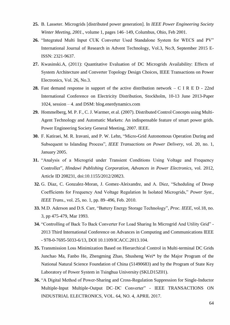
64
25. B. Lasseter. Microgrids [distributed power generation]. In IEEE Power Engineering Society
Winter Meeting, 2001., volume 1, pages 146–149, Columbus, Ohio, Feb 2001. 26. “Integrated Multi Input CUK Converter Used Standalone System for WECS and PV”
International Journal of Research in Advent Technology, Vol.3, No.9, September 2015 E-
ISSN: 2321-9637. 27. Kwasinski.A, (2011): Quantitative Evaluation of DC Microgrids Availability: Effects of
System Architecture and Converter Topology Design Choices, IEEE Transactions on Power
Electronics, Vol. 26, No.3. 28. Fast demand response in support of the active distribution network – C I R E D - 22nd
International Conference on Electricity Distribution, Stockholm, 10-13 June 2013-Paper
1024, session – 4. and DSM: blog.enerdynamics.com 29. Hommelberg, M. P. F., C. J. Warmer, et al. (2007). Distributed Control Concepts using Multi-
Agent Technology and Automatic Markets: An indispensable feature of smart power grids.
Power Engineering Society General Meeting, 2007. IEEE. 30. F. Katiraei, M. R. Iravani, and P. W. Lehn, “Micro-Grid Autonomous Operation During and
Subsequent to Islanding Process”, IEEE Transactions on Power Delivery, vol. 20, no. 1,
January 2005. 31. “Analysis of a Microgrid under Transient Conditions Using Voltage and Frequency
Controller”, Hindawi Publishing Corporation, Advances in Power Electronics, vol. 2012,
Article ID 208231, doi:10.1155/2012/20823. 32. G. Diaz, C. Gonzalez-Moran, J. Gomez-Aleixandre, and A. Diez, “Scheduling of Droop
Coefficients for Frequency And Voltage Regulation In Isolated Microgrids,” Power Syst.,
IEEE Trans., vol. 25, no. 1, pp. 89–496, Feb. 2010.
33. M.D. Aderson and D.S. Carr, “Battery Energy Storage Technology”, Proc. IEEE, vol.18, no.
3, pp 475-479, Mar 1993. 34. “Controlling of Back To Back Converter For Load Sharing In Microgrid And Utility Grid” -
2013 Third International Conference on Advances in Computing and Communications IEEE
- 978-0-7695-5033-6/13, DOI 10.1109/ICACC.2013.104. 35. Transmission Loss Minimization Based on Hierarchical Control in Multi-terminal DC Grids
Junchao Ma, Fanbo He, Zhengming Zhao, Shusheng Wei* by the Major Program of the
National Natural Science Foundation of China (51490683) and by the Program of State Key
Laboratory of Power System in Tsinghua University (SKLD15Z01). 36. “A Digital Method of Power-Sharing and Cross-Regulation Suppression for Single-Inductor
Multiple-Input Multiple-Output DC–DC Converter” - IEEE TRANSACTIONS ON
INDUSTRIAL ELECTRONICS, VOL. 64, NO. 4, APRIL 2017.
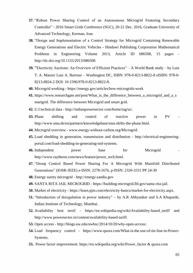
65
37. “Robust Power Sharing Control of an Autonomous Microgrid Featuring Secondary
Controller” - 2016 Smart Grids Conference (SGC), 20-21 Dec. 2016, Graduate University of
Advanced Technology, Kerman, Iran.
38. “Design and Implementation of a Control Strategy for Microgrid Containing Renewable
Energy Generations and Electric Vehicles - Hindawi Publishing Corporation Mathematical
Problems in Engineering Volume 2013, Article ID 686508, 15 pages -
http://dx.doi.org/10.1155/2013/686508.
39. “Electricity Auctions: An Overview of Efficient Practices” – A World Bank study – by Luiz
T. A. Maurer Luiz A. Barroso – Washington DC, ISBN: 978-0-8213-8822-8 eISBN: 978-0-
8213-8824-2 DOI: 10.1596/978-0-8213-8822-8.
40. Microgrid working - https://energy.gov/articles/how-microgrids-work
41. https://www.researchgate.net/post/What_is_the_difference_between_a_microgrid_and_a_s
martgrid. The difference between Microgrid and smart grid.
42. U.I technical data - http://indianpowersector.com/home/tag/ui/.
43. Phase shifting and control of reactive power in PV -
http://www.sma.de/en/partners/knowledgebase/sma-shifts-the-phase.html.
44. Microgrid overview - www.energy-without-carbon.org/Microgrid.
45. Load shedding in generation, transmission and distribution - http://electrical-engineering-
portal.com/load-shedding-in-generating-tnd-systems.
46. Independent power base for Microgrid -
http://www.raytheon.com/news/feature/power_tech.html.
47. “Droop Control Based Power Sharing For A Microgrid With Manifold Distributed
Generations” (IOSR-JEEE) e-ISSN: 2278-1676, p-ISSN: 2320-3331 PP 24-30
48. Energy surety microgrid - http://energy.sandia.gov
49. SANTA RITA JAIL MICROGRID - https://building-microgrid.lbl.gov/santa-rita-jail.
50. Market of electricity - https://learn.pjm.com/electricity-basics/market-for-electricity.aspx.
51. “Introduction of deregulation in power industry” – by A.R Abhyanker and S.A Khaparde,
Indian Institute of Technology, Mumbai.
52. Availability best terrif - https://en.wikipedia.org/wiki/Availability-based_tariff and
http://www.powersector.in/content/availability-based-tariff.
53. Open access - http://blogs.uw.edu/uwbsc/2014/10/20/why-open-access/.
54. Load frequency control - https://www.quora.com/What-is-the-use-of-tie-line-in-Power-
Systems.
55. Power factor improvement: https://en.wikipedia.org/wiki/Power_factor & quora.com
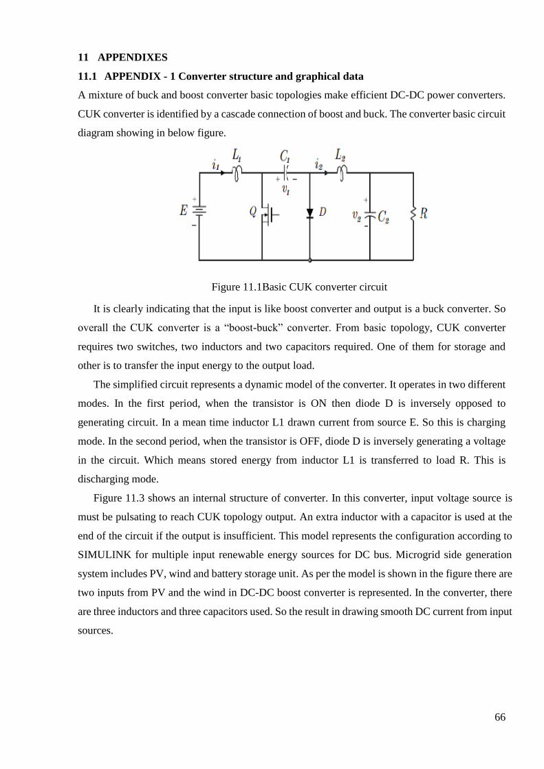
66
11 APPENDIXES
11.1 APPENDIX - 1 Converter structure and graphical data
A mixture of buck and boost converter basic topologies make efficient DC-DC power converters.
CUK converter is identified by a cascade connection of boost and buck. The converter basic circuit
diagram showing in below figure.
Figure 11.1Basic CUK converter circuit
It is clearly indicating that the input is like boost converter and output is a buck converter. So
overall the CUK converter is a “boost-buck” converter. From basic topology, CUK converter
requires two switches, two inductors and two capacitors required. One of them for storage and
other is to transfer the input energy to the output load.
The simplified circuit represents a dynamic model of the converter. It operates in two different
modes. In the first period, when the transistor is ON then diode D is inversely opposed to
generating circuit. In a mean time inductor L1 drawn current from source E. So this is charging
mode. In the second period, when the transistor is OFF, diode D is inversely generating a voltage
in the circuit. Which means stored energy from inductor L1 is transferred to load R. This is
discharging mode.
Figure 11.3 shows an internal structure of converter. In this converter, input voltage source is
must be pulsating to reach CUK topology output. An extra inductor with a capacitor is used at the
end of the circuit if the output is insufficient. This model represents the configuration according to
SIMULINK for multiple input renewable energy sources for DC bus. Microgrid side generation
system includes PV, wind and battery storage unit. As per the model is shown in the figure there are
two inputs from PV and the wind in DC-DC boost converter is represented. In the converter, there
are three inductors and three capacitors used. So the result in drawing smooth DC current from input
sources.
67
Figure 11.2 Ideal switching operation
Figure 11.3 Converter circuit from model
Model of converter
When u = 1,
𝐿1𝑑𝑖1
𝑑𝑡= 𝐸
𝐿2𝑑𝑖2
𝑑𝑡= −𝑣1 − 𝑣2 (11.1)
Capacitor voltage,
𝐶1𝑑𝑣1
𝑑𝑡= 𝑖2
𝐶2𝑑𝑣2
𝑑𝑡= 𝑖2 −
𝑣2
𝑅 (11.2)
When u=0
𝐿1𝑑𝑖1
𝑑𝑡= −𝑣1 + 𝐸
𝐿2𝑑𝑖2
𝑑𝑡= −𝑣2 (11.3)

68
Capacitor voltage v1 and v2 indicate by,
𝐶1𝑑𝑣1
𝑑𝑡= 𝑖1
𝐶2𝑑𝑣2
𝑑𝑡= 𝑖2 −
𝑣2
𝑅 (11.4)
Reference model partial equation,
𝐿1𝑑𝑖1
𝑑𝑡= −(1 − 𝑢)𝑣1 + 𝐸
𝐶1𝑑𝑣1
𝑑𝑡= (1 − 𝑢)𝑖1 + 𝑣𝑖2
𝐿2𝑑𝑖2
𝑑𝑡= −𝑢𝑣1 − 𝑣2
𝐶2𝑑𝑣1
𝑑𝑡= 𝑖2 −
𝑣2
𝑅 (11.5)
From figure 12.2, u1 and i1 are voltage and current across C1 and L1 respectively. Other u2
across the capacitor C2 and load R and i2 across inductor L2. The voltage source E is constant.
Steady state analysis of CUK converter
Voltage (current) step-up and step-down capability, controlled by duty ratio D.
Combines goof characteristics of buck and boost converters (input and output voltage filtering).
Coupling capacitor
Figure 11.4 Schematic diagram of CUK converter
Power transfer through the coupling capacitor Cc.
Cc is assumed large enough to approximate its voltage to be constant DC in steady state.
It is not larger then output capacitor and ripple in the voltage is higher.
Voltage polarity in steady state is as shown in the schematic diagram.
Inductor on both input and output side ensures that current are not pulsating.
Switch on interval
As per the equivalent circuit, the switch S1 is on and diode D1 is in reverse bias. Because of the
large voltage of Vcc when the switch S1 is on and the path has short-circuited the current in the
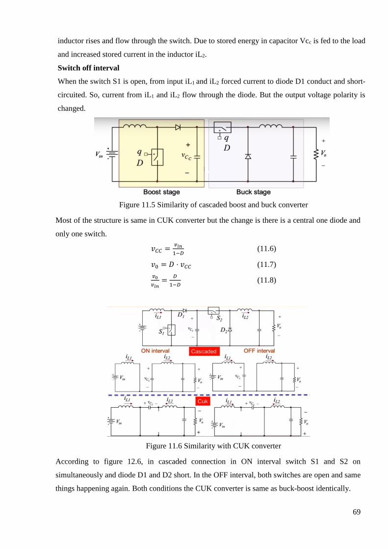
69
inductor rises and flow through the switch. Due to stored energy in capacitor Vcc is fed to the load
and increased stored current in the inductor iL2.
Switch off interval
When the switch S1 is open, from input iL1 and iL2 forced current to diode D1 conduct and short-
circuited. So, current from iL1 and iL2 flow through the diode. But the output voltage polarity is
changed.
Figure 11.5 Similarity of cascaded boost and buck converter
Most of the structure is same in CUK converter but the change is there is a central one diode and
only one switch.
𝑣𝐶𝐶 =𝑣𝑖𝑛
1−𝐷 (11.6)
𝑣0 = 𝐷 ⋅ 𝑣𝐶𝐶 (11.7)
𝑣0
𝑣𝑖𝑛=
𝐷
1−𝐷 (11.8)
Figure 11.6 Similarity with CUK converter
According to figure 12.6, in cascaded connection in ON interval switch S1 and S2 on
simultaneously and diode D1 and D2 short. In the OFF interval, both switches are open and same
things happening again. Both conditions the CUK converter is same as buck-boost identically.
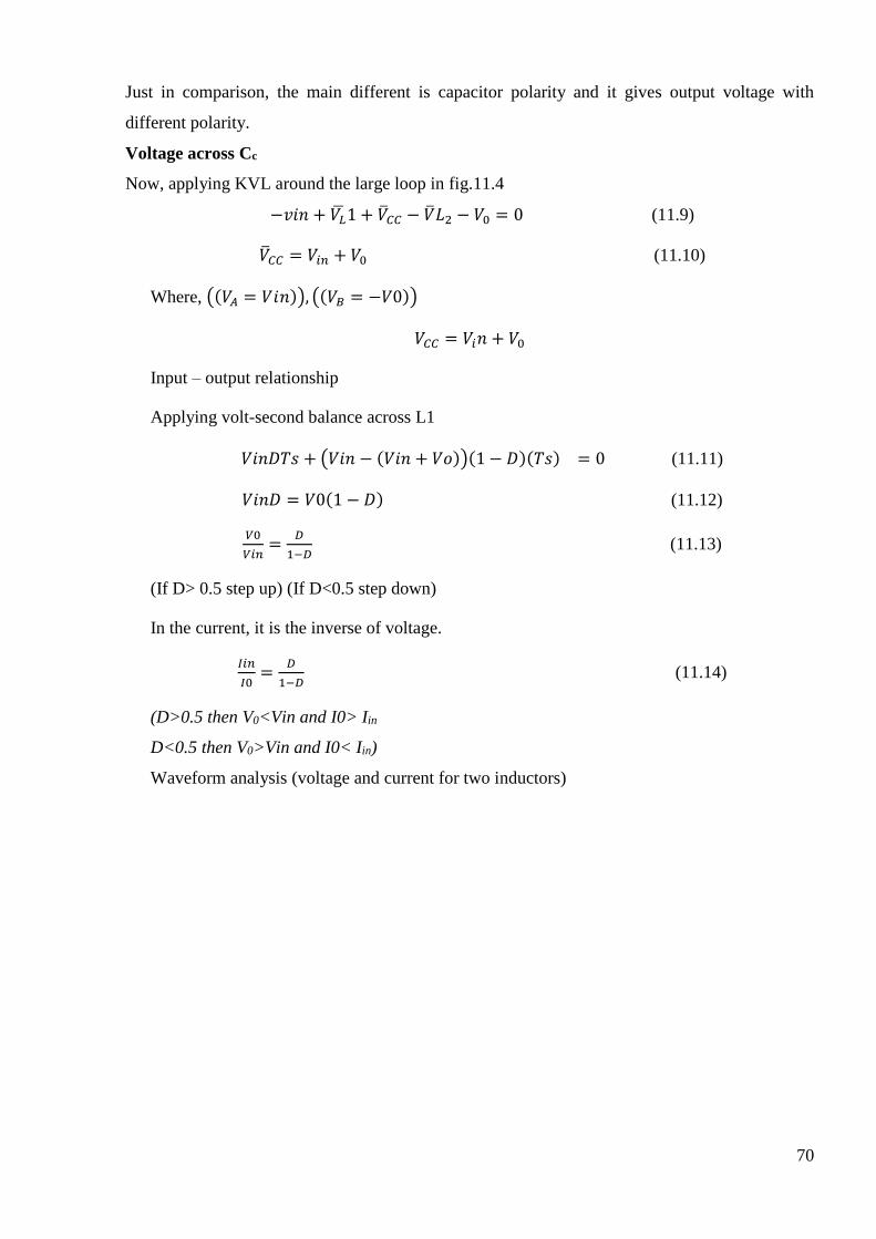
70
Just in comparison, the main different is capacitor polarity and it gives output voltage with
different polarity.
Voltage across Cc
Now, applying KVL around the large loop in fig.11.4
−𝑣𝑖𝑛 + 𝑉�̅�1 + �̅�𝐶𝐶 − �̅�𝐿2 − 𝑉0 = 0 (11.9)
�̅�𝐶𝐶 = 𝑉𝑖𝑛 + 𝑉0 (11.10)
Where, ((𝑉𝐴 = 𝑉𝑖𝑛)), ((𝑉𝐵 = −𝑉0))
𝑉𝐶𝐶 = 𝑉𝑖𝑛 + 𝑉0
Input – output relationship
Applying volt-second balance across L1
𝑉𝑖𝑛𝐷𝑇𝑠 + (𝑉𝑖𝑛 − (𝑉𝑖𝑛 + 𝑉𝑜))(1 − 𝐷)(𝑇𝑠) = 0 (11.11)
𝑉𝑖𝑛𝐷 = 𝑉0(1 − 𝐷) (11.12)
𝑉0
𝑉𝑖𝑛=
𝐷
1−𝐷 (11.13)
(If D> 0.5 step up) (If D<0.5 step down)
In the current, it is the inverse of voltage.
𝐼𝑖𝑛
𝐼0=
𝐷
1−𝐷 (11.14)
(D>0.5 then V0<Vin and I0> Iin
D<0.5 then V0>Vin and I0< Iin)
Waveform analysis (voltage and current for two inductors)

71
Figure 11.7 Voltage and current waveform analysis
−𝐼𝑜𝐷𝑇𝑆 + 𝐼𝑖𝑛(1 − 𝐷)𝑇𝑠 = 0 (11.15)
𝐼 𝑖(1 − 𝐷) = 𝐼𝑜𝐷 (11.16)
𝐼𝑖𝑛
𝐼0=
𝐷
1−𝐷 (11.17)
Graphical represents results from SIMULINK with and without converter
As per the simulation results here there are some different parameters readings which are showing
the difference without a converter and with converter, what effect is showing on the system.
Graph 11.1 Battery current with charge controller – (before-after)
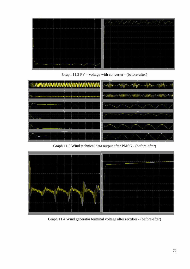
72
Graph 11.2 PV – voltage with converter - (before-after)
Graph 11.3 Wind technical data output after PMSG - (before-after)
Graph 11.4 Wind generator terminal voltage after rectifier - (before-after)

73
Graph 11.5 Battery voltage, current and SOC%
Graph 11.6 Battery discharging characteristics and generator terminal FFT analysis
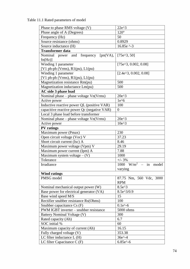
74
Table 11.1 Rated parameters of model
Phase to phase RMS voltage (V) 22e^3
Phase angle of A (Degrees) 120°
Frequency (Hz) 50
Source resistance (ohms) 0.8929
Source inductance (H) 16.85e ^-3
Transformer data
Nominal power and frequency [pn(VA),
fn(Hz)]
[75e^3, 50]
Winding 1 parameter
[V1 ph-ph (Vrms), R1(pu), L1(pu)
[75e^3, 0.002, 0.08]
Winding 1 parameter
[V1 ph-ph (Vrms), R1(pu), L1(pu)
[2.4e^3, 0.002, 0.08]
Magnetization resistance Rm(pu) 500
Magnetization inductance Lm(pu) 500
AC side 3 phase load
Nominal phase – phase voltage Vn(Vrms) 20e^3
Active power 1e^6
Inductive reactive power QL (positive VAR) 100
capacitive reactive power Qc (negative VAR) 0
Local 3 phase load before transformer
Nominal phase – phase voltage Vn(Vrms) 20e^3
Active power 10e^3
PV ratings
Maximum power (Pmax) 230
Open circuit voltage (Voc) V 37.23
Short circuit current (Isc) A 8.46
Maximum power voltage (Vpm) V 29.19
Maximum power current (Ipm) A 7.88
Maximum system voltage – (V) 1000
Tolerance +/- 3%
Irradiance 1000 W/m2 – in model
varying
Wind ratings
PMSG model 87.75 Nm, 560 Vdc, 3000
RPM
Nominal mechanical output power (W) 8.5e^3
Base power for electrical generator (VA) 8.5e^3/0.9
Base wind speed M/S 15
Rectifier snubber resistance Rs(Ohms) 100
Snubber capacitance Cs (F) 0.1e^-6
PWM IGBT inverter – snubber resistance 5000 ohms
Battery Nominal Voltage (V) 300
Rated capacity (Ah) 6.7
SOC initial % 60
Maximum capacity of current (Ah) 16.15
Fully charged voltage (V) 353.38
LC filter inductance L (H) 36e^-4
LC filter Capacitance C (F) 6.85e^-6

75
11.2 APPENDIX – 2 Programming and readings
The table shows the data of U.I rate according to frequency up and down.
These readings are taken by SLDC from India.
Table 11.2 U.I rate with frequency
Average fq of time
block in (Hz)
U.I rate - (Paisa PER KW)
50.05 0
50.04 35.69
50.03 71.28
50.02 106.87
50.01 142.46
50 178
49.99 198.80
49.98 219.63
49.97 240.98
49.96 261.39
49.95 282.20
49.94 303.04
49.93 323.89
49.92 344.75
49.91 365.58
49.90 386.40
49.89 407.83
49.88 428.10
49.87 448.90
49.86 469.78
49.85 490.61
49.84 511.45
49.83 532.28
49.82 553.14
49.81 573.91
49.80 594.80
49.79 615.65
49.78 634.48
49.77 657.30
49.76 678.18
49.75 699
49.74 719.85
49.73 740.67
49.72 761.52
49.71 782.36
49.70 803.20
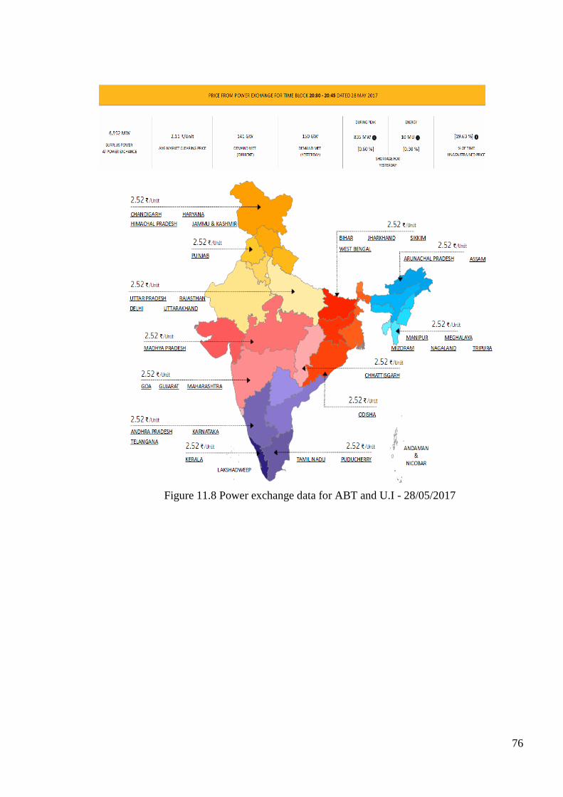
76
Figure 11.8 Power exchange data for ABT and U.I - 28/05/2017

77
Programming for impact on Microgrid due to PV in MATLAB/SIMULINK for graph 8.4
% 26-04-2017 % Harsh Patel % This script loads home consumption data from % .CSV files. At the end, the consumption of each house % is available in the workspace (e.g., 'house01.mat'). % The column headers in the .CSV file are: % ----------------------------------------------------------- % Date & Time Use [kW] Gen [kW] Grid [kW] Solar [kW] % (col 1 col2 col3 col4 col5) % ----------------------------------------------------------- % col 1 = date and time stamp in '26/04/2017 02;31' format % col 2 = house power usage (Phouse, kW) % col 3 = (same as col 5) % col 4 = net power consumption as seen from the grid (Pgrid, kW) % col 5 = power generated by solar panel (Psolar, kW) % Power balance relation: % Pgrid + Psolar = Phouse % where: % Pgrid = see col 4 % Psolar = see col 5 % Phouse = see col 2 clc close all clear % Create a figure in the maximized position hFigure = figure('Position', get(0,'ScreenSize')); % Load data for 12 homes for i=1:12 % Prefix variable 'i' with a '0' % to get i=01,02,03... instead of i=1,2,3 zeroPrefix = '0'; if (i>=10) zeroPrefix = ''; % do not prefix numbers >=10 end % Create a home's variable name % (e.g., 'house01') houseName = ['house' zeroPrefix num2str(i)];
% Create the .CSV file name % (e.g., 'house01.csv') fileName = [houseName '.csv'];
% Read the house data from the .CSV file % (parameters 1,1 = imports .CSV data % starting at row 1, col 1) houseData = csvread(fileName, 1,1);
% Extract individual columns % (['] converts a column to a row) phouse = houseData(:,1)'; % col 2 in .CSV file pgrid = houseData(:,3)'; % col 4 in .CSV file psolar = houseData(:,4)'; % col 5 in .CSV file % Create a time array in seconds numPoints = length(phouse); dt = 60; % time increment = 60 s timeInSeconds = dt*(0:numPoints-1);

78
% Create time array in hours % (used to show hours on X axis of the plots) timeInHours = timeInSeconds./3600;
% Plot the house data hFigure = subplot(3,4,i); % create a 3 x 4 figure hold on plot(timeInHours, pgrid, 'b'); % plot power seen from grid plot(timeInHours, psolar, 'g'); % plot power generator from PV plot(timeInHours, phouse, 'r'); % plot house consumption
% Add plot labels grid on; legend({'P_{grid}','P_{solar}','P_{house}'}); title(['House ', num2str(i)]); xlabel('Time (hours)'); ylabel('kW'); axis([0, 25, -5, 15])
% Save the house data to the workspace. This data is % used by Simulink during the simulation. % Simulink requires that the time be in seconds and in column 1. % col 1: time in seconds % col 2: grid power (Pgrid). % % The following command creates a structure in the workspace with % the two aforementioned columns. eval([houseName ' = [timeInSeconds'' pgrid''];']); end % Clean up temp variables clear phouse clear pgrid clear psolar clear timeInHours clear houseName clear houseData clear i clear numPoints clear timeInSeconds clear zeroPrefix clear dt clear fileName