Embed Size (px)
Citation preview
This is an electronic reprint of the original article.This reprint may differ from the original in pagination and typographic detail.
Powered by TCPDF (www.tcpdf.org)
This material is protected by copyright and other intellectual property rights, and duplication or sale of all or part of any of the repository collections is not permitted, except that material may be duplicated by you for your research use or educational purposes in electronic or print form. You must obtain permission for any other use. Electronic or print copies may not be offered, whether for sale or otherwise to anyone who is not an authorised user.
Karak, Bidya Binay; Rheinhardt, Matthias; Brandenburg, Axel; Käpylä, Petri; Käpylä, Maarit J.
Quenching and anisotropy of hydromagnetic turbulent transport
Published in:Astrophysical Journal
DOI:10.1088/0004-637X/795/1/16
Published: 01/01/2014
Document VersionPublisher's PDF, also known as Version of record
Please cite the original version:Karak, B. B., Rheinhardt, M., Brandenburg, A., Käpylä, P. J., & Käpylä, M. J. (2014). Quenching and anisotropyof hydromagnetic turbulent transport. Astrophysical Journal, 795(1). https://doi.org/10.1088/0004-637X/795/1/16

The Astrophysical Journal, 795:16 (16pp), 2014 November 1 doi:10.1088/0004-637X/795/1/16C© 2014. The American Astronomical Society. All rights reserved. Printed in the U.S.A.
QUENCHING AND ANISOTROPY OF HYDROMAGNETIC TURBULENT TRANSPORT
Bidya Binay Karak1, Matthias Rheinhardt2, Axel Brandenburg1,3, Petri J. Kapyla2,4, and Maarit J. Kapyla41 Nordita, KTH Royal Institute of Technology and Stockholm University, Roslagstullsbacken 23, SE-10691 Stockholm, Sweden
2 Department of Physics, Gustaf Hallstromin katu 2a, P.O. Box 64, FI-00014 University of Helsinki, Finland3 Department of Astronomy, AlbaNova University Center, Stockholm University, SE-10691 Stockholm, Sweden
4 ReSoLVE Centre of Excellence, Department of Information and Computer Science, Aalto University, P.O. Box 15400, FI-00076 Aalto, FinlandReceived 2014 June 17; accepted 2014 August 20; published 2014 October 9
ABSTRACT
Hydromagnetic turbulence affects the evolution of large-scale magnetic fields through mean-field effects liketurbulent diffusion and the α effect. For stronger fields, these effects are usually suppressed or quenched, andadditional anisotropies are introduced. Using different variants of the test-field method, we determine the quenchingof the turbulent transport coefficients for the forced Roberts flow, isotropically forced non-helical turbulence, androtating thermal convection. We see significant quenching only when the mean magnetic field is larger than theequipartition value of the turbulence. Expressing the magnetic field in terms of the equipartition value of thequenched flows, we obtain for the quenching exponents of the turbulent magnetic diffusivity about 1.3, 1.1, and 1.3for Roberts flow, forced turbulence, and convection, respectively. However, when the magnetic field is expressed interms of the equipartition value of the unquenched flows, these quenching exponents become about 4, 1.5, and 2.3,respectively. For the α effect, the exponent is about 1.3 for the Roberts flow and 2 for convection in the first case,but 4 and 3, respectively, in the second. In convection, the quenching of turbulent pumping follows the same powerlaw as turbulent diffusion, while for the coefficient describing the Ω × J effect nearly the same quenching exponentis obtained as for α. For forced turbulence, turbulent diffusion proportional to the second derivative along the meanmagnetic field is quenched much less, especially for larger values of the magnetic Reynolds number. However, wefind that in corresponding axisymmetric mean-field dynamos with dominant toroidal field the quenched diffusioncoefficients are the same for the poloidal and toroidal field constituents.
Key words: convection – diffusion – dynamo – magnetic fields – magnetohydrodynamics (MHD) – turbulence
Online-only material: color figures
1. INTRODUCTION
Many astrophysical objects possess turbulent convection,and the dynamo mechanisms based on it are believed to beresponsible for the generation and maintenance of the observedmagnetic fields. The study of the dynamo mechanism in thesolar convection zone using simulations of turbulent convectionin spherical shells began in the 1980s with the works of Gilman& Miller (1981), Gilman (1983), and Glatzmaier (1985), andhas recently been pursued further by many more authors (Brunet al. 2004; Racine et al. 2011; Kapyla et al. 2012, 2013; Karaket al. 2014). However, under stellar conditions the dimensionlessparameters governing magnetohydrodynamics attain extremevalues, which are far from being accessible through numericalmodels. So we do not know to what extent feasible models attemperate parameter regimes reflect properties of convectionand dynamos in real stars. An alternative approach to studyingthe dynamo problem is mean-field theory, which began withthe pioneering works of Parker (1955), Braginsky (1964), andSteenbeck et al. (1966). This approach is computationallyless expensive because one does not need to resolve thefull dynamical range of the small-scale turbulence, whichis instead parameterized. In recent years, there have beensignificant achievements of mean-field MHD in reproducingvarious aspects of magnetic and flow fields in the Sun (e.g.,Chatterjee et al. 2004; Rempel 2006; Kapyla et al. 2006;Choudhuri & Karak 2009, 2012; Karak 2010; Charbonneau2010; Pipin & Kosovichev 2011).
In this context, an important task is to determine the meanelectromotive force E , which results from the correlation be-
tween the fluctuating constituents of velocity and magnetic field,in terms of the mean field B. There is no accurate theory toaccomplish this task from first principles, except for some lim-iting cases, in particular those of small Strouhal and magneticReynolds number, Rm. Therefore, suitable assumptions are re-quired in determining E . When B varies slowly in space andtime, we may write
E i = αijBj + βijk
∂Bj
∂xk
. (1)
The diagonal components of αij are usually the most importantterms for dynamo action, but in the presence of shear, the Ω × J(Krause & Radler 1980) and shear-current (Rogachevskii &Kleeorin 2003) effects, both covered by βijk , can also enable it.Many components of βijk , however, describe dissipative effects.
Doubts can be raised regarding the explanatory and predictivepower of mean-field dynamo models given that the tensorsαij and βijk are often chosen to some extent arbitrarily orare even tuned to obtain results resembling features of theSun. Therefore, methods to measure these coefficients fromsimulations have been developed. At present the most accuratemethod is the so-called test-field method (Schrinner et al. 2005,2007; Brandenburg et al. 2008b, 2013). In this method, oneselects an adequate number of independent mean fields, the “testfields,” and solves for each of them the corresponding equationfor the fluctuating magnetic field (in addition to the mainsimulation). Finally, via computing the mean electromotiveforce, the transport coefficients are calculated.
There are different variants of the test-field method. The bestestablished one is based on the average over two spatial (the
1

The Astrophysical Journal, 795:16 (16pp), 2014 November 1 Karak et al.
“horizontal”) coordinates. This method has been applied to alarge variety of setups, e.g., isotropic homogeneous turbulence(Sur et al. 2008; Brandenburg et al. 2008b), homogeneous shearflow turbulence (Brandenburg et al. 2008a), with and withouthelicity (Mitra et al. 2009), turbulent convection (Kapyla et al.2009a), and supernova-driven interstellar turbulence (Gresselet al. 2013). Another variant is based on Fourier-weighted hor-izontal averages and allows us to determine also the coeffi-cients that multiply horizontal derivatives of the mean field.This method has been applied to forced turbulence (Brandenburget al. 2012) and to cosmic-ray-driven turbulence (Rogachevskiiet al. 2012; Bykov et al. 2013).
In dynamo models based on thin flux tubes, forming themajor alternative to distributed turbulent dynamos, the magneticfield strength in the deep parts of the solar convection zoneis believed to exceed its value at equipartition with velocity(Choudhuri & Gilman 1987; D’Silva & Choudhuri 1993; Weberet al. 2011). On the other hand, it is well known that turbulenttransport becomes less efficient when the mean magnetic field’sstrength is comparable to or larger than the equipartition value.Therefore, precise knowledge of this “quenching” is needed.Mean-field dynamo models of the αΩ type often employ an“ad hoc” algebraic or dynamical α-quenching (Jepps 1975;Covas et al. 1998), while largely ignoring the quenching of theturbulent diffusivity ηt despite its importance in determiningthe cycle frequency. Indeed, in the absence of quenching, thestandard estimate of ηt for the Sun (∼1012–1013 cm2 s−1) yieldsa rather short cycle period of 2–3 yr (Kohler 1973). However, byconsidering the quenching of ηt , a reasonable value of the cycleperiod can easily be obtained (Rudiger et al. 1994; Guerreroet al. 2009; Munoz-Jaramillo et al. 2011). In fact, measuring thecycle frequency in a simulation has been one way of determiningthe quenching of ηt (Kapyla & Brandenburg 2009).
Early work by Moffatt (1972) and Rudiger (1974) showed thatunder the Second Order Correlation Approximation (SOCA),α is quenched inversely proportional to the third power ofthe magnetic field. Following Vainshtein & Cattaneo (1992),several investigations have suggested that α is beginning to bequenched noticeably when the mean field becomes comparableto R−1
m times the equipartition value (Cattaneo & Hughes1996), i.e., for extremely weak magnetic fields. This behavioris also called “catastrophic quenching.” However, it is nowunderstood as an artifact of having defined volume-averagedmean fields (Brandenburg 2001; Brandenburg et al. 2008b)combined with the usage of perfectly conducting or periodicboundary conditions and is not expected to be important inastrophysical bodies where magnetic helicity fluxes can alleviatecatastrophic quenching (e.g., Kleeorin et al. 2000; Del Sordoet al. 2013). The actual value of α shows a much weakerdependence on Rm even when B is comparable with theequipartition value (Brandenburg et al. 2008b). This work alsoshows that the Rm dependence of α and ηt is such that ina saturated state their contributions to the growth rate nearlybalance, with a residual matching the microscopic resistiveterm. Consequently, the saturated mean electromotive forceis proportional to R−1
m , which is sometimes misinterpreted ascatastrophic quenching.
Once catastrophic quenching is alleviated, the magnetic fieldcan grow to equipartition field strengths, when other quenchingmechanisms that are not Rm dependent might become importantand can therefore be studied already for smaller values of Rm.
Sur et al. (2007) found that α is quenched proportional to 1/B2
and 1/B3
for time-dependent and steady flows, respectively.Their latter result was based on analytic theory and appeared tobe confirmed by numerical simulations using a steady forcingproportional to the ABC-flow. However, subsequent work byRheinhardt & Brandenburg (2010) demonstrated quenching
proportional to B−4
for a steady forcing proportional to theflow I of Roberts (1972), hereafter referred to as Roberts flow.They also noted that for ABC-flow forcing the quenching isindeed better described when setting the power also to 4 insteadof 3. More recently, in supernova-driven turbulent dynamosimulations, Gressel et al. (2013) find α ∼ (B/Beq)−2, whereBeq is the local equipartition value.
For the turbulent diffusivity, Kitchatinov et al. (1994) andRogachevskii & Kleeorin (2000) obtained that ηt is quenchedinversely proportional to B. In the two-dimensional case,Cattaneo & Vainshtein (1991) have found catastrophic quench-ing of ηt . However, this is a special situation connected withthe fact that in two dimensions the mean square vector poten-tial is a conserved quantity. This is no longer the case in threedimensions. Quenching similar to Kitchatinov et al. (1994) hasbeen confirmed by simulations (Brandenburg 2001; Blackman& Brandenburg 2002; Gressel et al. 2013). In particular, makingthe ansatz ηt ∼ 1/
(1 + p(B/Beq)q
), Gressel et al. (2013) find
q ≈ 1 in supernova-driven simulations of the turbulent interstel-lar medium. On the other hand, Yousef et al. (2003) find q ≈ 2in simulations of forced turbulence with a decaying large-scalemagnetic field. However, Kapyla & Brandenburg (2009) foundthat their results depend on the strength of shear with q ≈ 1 forweak shear while q ≈ 2 for strong shear.
In the present work we measure the quenching of thesetransport coefficients as a function of the mean magnetic fieldstrength for three different background simulations: (1) forcedRoberts flow, (2) forced turbulence in a triply periodic box, and(3) convection in a bounded box. In all these simulations, weimpose a uniform and constant external mean field. However,this induces a preferred direction that causes the statisticalproperties of the turbulence to be axisymmetric with respectto the direction of the magnetic field. In the following, we referto such flows as axisymmetric turbulence, for which the numberof independent components of the α and η tensors is reducedto only nine, simplifying also their determination (Brandenburget al. 2012).
2. CONCEPT OF TURBULENT TRANSPORT INMEAN-FIELD DYNAMO
The evolution of the magnetic field B in an electricallyconducting fluid is governed by the induction equation
∂ B∂t
= ∇ × (U × B − η J), (2)
where U is the fluid velocity. Here, η is the microphysicalmagnetic diffusivity, while the magnetic permeability of thefluid has been set to unity. Thus, the current density J is givenby J = ∇ × B. In mean-field MHD, we consider the fields assums of “averaged” and small-scale “fluctuating” fields, with theassumption that the averaging satisfies (at least approximately)the Reynolds rules. Denoting averaged fields by overbars andfluctuating ones by lowercase letters, we write the equation forthe mean magnetic field B as
∂ B∂t
= ∇ × (U × B + E − η J
), (3)
2

The Astrophysical Journal, 795:16 (16pp), 2014 November 1 Karak et al.
where E = u × b is the aforementioned mean electromotiveforce, which captures the correlation of the fluctuating fields uand b. The ultimate goal of mean-field MHD is to express E interms of B itself. There are several procedures for doing that.When the mean magnetic field varies slowly in space and timewe can write E in the form of Equation (1). Our primary goal isto measure the transport coefficients αij and βijk in the presenceof an imposed uniform magnetic field Bext and, in particular, tomeasure the degree of their quenching and anisotropy.
Let us consider turbulence that is anisotropic and exhibitingonly one preferred direction e, referring to an external magneticfield, rotation axis, or the direction of gravity. Then followingBrandenburg et al. (2012), the general representation of E isgiven by
E = α⊥ B + (α‖ − α⊥)(e · B)e + γ e × B
− η⊥ J − (η‖ − η⊥)(e · J)e − δ e × J
− κ⊥ K − (κ‖ − κ⊥)(e · K )e − μe × K (4)
with nine coefficients α⊥, α‖, . . ., μ. While J is given by theantisymmetric part of the gradient tensor ∇B, K is defined byK = e · (∇B)S, with (∇B)S being the symmetric part of ∇B.For homogeneous isotropic turbulence, α‖ = α⊥, η‖ = η⊥, andthe other coefficients vanish. We note that our sign conventionfor α⊥, α‖, and γ follows that commonly used, but it differsfrom that used in Brandenburg et al. (2012).
The μ term corresponds to a modification of turbulentdiffusion along the preferred direction. To understand this,let us assume that only η⊥, η‖, and μ are non-vanishingand independent of position. By introducing the quantitiesηT ≡ ηt + η, with ηt ≡ η⊥ − μ/2, and ε ≡ η‖ − η⊥ + μ/2, wehave
∂ B∂t
= ηT ∇2 B + μ∇2‖ B + ε
(∇2
⊥ B⊥ + ∇⊥∇‖B‖), (5)
which shows that positive values of μ correspond to an en-hancement of turbulent diffusion along the preferred direction.As Equation (5) reveals, η‖ and η⊥ do not characterize the dif-fusion parallel and perpendicular to the preferred direction, astheir symbols might suggest.
An anisotropy similar to that of Equation (5) has beenconsidered in connection with the turbulent decay of sunspotmagnetic fields (Rudiger & Kitchatinov 2000), where the meanmagnetic field defines the preferred direction. It has not yetbeen used in mean-field dynamo models, where, however,anisotropies of the turbulent diffusivity due to the simultaneousinfluence of rotation and stratification have been taken intoaccount (Rudiger & Brandenburg 1995; Pipin & Kosovichev2014).
3. THE MODEL SETUP
We distinguish two basically different schemes of establish-ing the background flow: by a prescribed forcing or by theconvective instability. In the first case, both laminar and turbu-lent (artificially forced) flows will be considered. With respect tothe fluid, we generally think of an ideal gas with state variablesdensity ρ, pressure p, and temperature T, adopting, however,different effective equations of state for the two schemes.
The continuity and induction equations are shared by bothschemes and take the form
D ln ρ
Dt= −∇ · U, (6)
∂ A∂t
= U × B + η∇2 A. (7)
Here D/Dt = ∂/∂t + U ·∇ is the advective time derivative andA is the magnetic vector potential. The magnetic field includesthe imposed field, i.e., B = Bext + ∇ × A, and the microscopicdiffusivity η is constant.
3.1. Forced Flows
In these models, we assume the fluid to be isothermal, whichimplies for its equation of state p = c2
s ρ, with the constantsound speed cs. Hence, we solve Equations (6) and (7) togetherwith the momentum equation,
DUDt
= −c2s ∇ ln ρ + ρ−1( J × B + ∇·2ρνS) + f . (8)
Here ν = const is the kinematic viscosity, and f is a forcingfunction to be specified below. The traceless rate of strain tensorS is given by
Sij = 12 (Ui,j + Uj,i) − 1
3δij∇ · U, (9)
where the commas denote partial differentiation with respect tothe coordinate j or i.
The simulation domain for this model is periodic in alldirections with dimension Lx × Ly × Lz. In the following wealways use Lx = Ly ≡ L and express lengths in units of theinverse of the wavenumber k1 = 2π/L.
3.1.1. Roberts Forcing
First, we use a laminar forcing to maintain one of the flowsfor which Roberts (1972) had demonstrated dynamo action,namely, his flow I. It is incompressible, independent of z, andall second-rank tensors obtained from it by xy averaging aresymmetric about the z-axis (Radler et al. 2002). The flow isdefined by
u0 = −z × ∇ψ + kf ψ z , (10)
where
ψ = (u0/k0) cos k0x cos k0y , kf =√
2 k0 , (11)
with constant u0 and k0. Note that this flow is maximally helical,i.e., ∇ × u0 = kf u0. We define the forcing f such that forB = 0, the flow (10) with ρ = ρ0 = const is an exact solutionof Equation (8):
f = νk20 u0 + u0 · ∇u0
(=νk20 u0 + 1
2∇u20
). (12)
We perform several simulations with different strengths of theexternal magnetic field Bext with this forcing.
3.1.2. Forced Turbulence
Here we employ for f a random forcing function, namely,a linearly polarized wave with wavevector and phase beingchanged randomly between integration timesteps (Brandenburg2001). The driven flow is non-helical and known to lack an αeffect (Brandenburg et al. 2008a). The averaged modulus of thewavevector is denoted by kf , and the ratio kf /k1 is referred toas the scale separation ratio. To achieve sufficiently large scaleseparation, we would need to keep kf /k1 large. However, inthis case Rm = urms/ηkf becomes small. Therefore, we usekf /k1 � 5 as a compromise.
3

The Astrophysical Journal, 795:16 (16pp), 2014 November 1 Karak et al.
3.2. Convection
In this model the background flow is generated by convectionand consequently we employ p = (cp − cv)ρT for the equationof state of the fluid, where cp and cv are the specific heats atconstant pressure and volume, respectively. Our model is similarto many earlier studies in the literature (e.g., Brandenburg et al.1996; Ossendrijver et al. 2001; Kapyla et al. 2008; Kapyla et al.2009a, 2009b). Its computational domain is a rectangular boxconsisting of three layers: the lower part (−0.85 � z/d < 0) is aconvectively stable overshoot layer, the middle part (0 � z/d �1) is convectively unstable, and the upper part (1 < z/d � 1.15)is an almost isothermal cooling layer. The overshoot layer wasmade comparatively thick to guarantee that the overshooting isnot affected by the lower boundary. The box dimensions are(Lx,Ly, Lz) = (5, 5, 2)d, where d is the depth of the unstablelayer. Gravity is acting in the downward direction (i.e., alongthe negative z direction). By including rotation about the z-axis,we can consider the simulation box as a small portion of a starlocated at one of its poles. The mass conservation and inductionequations (6) and (7) are now complemented by a modifiedmomentum equation and an equation for the internal energy perunit mass (Brandenburg et al. 1996)
DUDt
= −∇p
ρ+ g − 2Ω × U +
1
ρ( J × B + ∇ · 2νρS),
De
Dt= −p
ρ∇· U +
1
ρcv
∇·K(z)∇e + 2νS2 +ημ0
ρJ2 − e−e0
τ (z).
(13)
Here, g = −g z, with g > 0, is the gravitational acceleration;Ω = Ω0(− sin θ, 0, cos θ ) is the rotation vector, with θ its angleagainst the z direction; and K is the heat conductivity with apiecewise constant z profile to be specified below. The specificinternal energy is related to the temperature via e = cvT . Inthe energy equation (13), the last term is of relaxation typeand regulates the internal energy to settle on average close toe0 = const. As there is permanent heat input from the lowerboundary and from viscous heating, it effectively acts as acooling. The relaxation rate τ (z)−1 has a value of 75
√g/d within
the cooling layer and drops smoothly to zero within the unstablelayer over a transition zone of width 0.025d.
The vertical boundary conditions for the velocity are chosento be impenetrable and stress free, i.e.,
Ux,z = Uy,z = Uz = 0, (14)
while for the magnetic field we use the vertical field boundarycondition Bx = By = 0. A steady influx of heat F0 =−(K∂ze)(x, y,−0.85d)/cv at the bottom of the box and aconstant temperature, i.e., constant internal energy, at its topare maintained, where the latter is specified to be just equal toe0 occurring in the relaxation term. The x and y directions areperiodic for all fields.
The input parameters are now determined in the followingsomewhat indirect way: Instead of prescribing K, it is assumedthat the hydrostatic reference solution coincides in the overshootand unstable layers with a polytrope, the index m of which isprescribed. Here we choose m = 3 and m = 1, respectively.As for a polytrope de/dz = −g/(m + 1)(γ − 1), γ = cp/cv ,and at each z we have F0 = −(K/cv)de/dz = const, the heatconductivity is obtained as K = cv(m + 1)(γ −1)F0/g, i.e., it isalso piecewise constant (for a physical motivation, see Hurlburtet al. 1986). For simplicity it is assumed that in the cooling
layer, for which no polytrope exists, K has the same valueas in the unstable one. Within the ranges of the other controlparameters covered by our simulations, it is then guaranteed thatthe relaxation to the quasi-isothermal state is dominated by theterm −e/τ .
The convection problem is governed by a set of dimensionlesscontrol parameters comprising the Prandtl, Taylor, and Rayleighnumbers
Pr = ν
χ (zm), Ta = 4Ω2d4
ν2, (15)
Ra = gd4
νχ (zm)Hp(zm)Δ∇(zm), (16)
along with the dimensionless pressure scale height at the top
ξ0 = (γ − 1)e0/gd. (17)
For the calculation of the Prandtl and Rayleigh numbers, thevalues of the thermal diffusivity χ = K/ρcp, the superadiabaticgradient Δ∇ = d(s/cP )/d ln p and the pressure scale height Hpof the associated hydrostatic equilibrium solution are taken fromthe middle of the convective layer at zm = d/2. The densitycontrast within the unstable layer is
ρ(0)
ρ(d)= 1 +
gd
2(γ − 1)e0= 1 +
1
2ξ0. (18)
Hence, the parameter ξ0 controls the density stratification inour domain. We use ξ0 = 3/25 in all the simulations, whichresults in a (hydrostatic) density contrast of 31/6; γ was fixedto 5/3 throughout, and the different models have the same initialdensity at z = zm.
Equation (18) assumes that e = e0 at the top of the convectivelayer, which cannot be exactly true. In the simulations this erroris increased by the fact that the effect of the cooling reachessomewhat below z/d = 1. This leads to a higher density contrast(≈8) in the actual hydrostatic solution.
3.3. Diagnostics
As diagnostics we use the fluid and magnetic Reynoldsnumbers
Re = urms
νkf
, Rm = urms
ηkf
, (19)
where for the convection setup kf = 2π/d is an estimate ofthe wavenumber of the largest energy-carrying eddies. urms =〈u2〉1/2 is the rms value of the velocity, with 〈·〉 denoting theaverage over the whole box or, for the convection setup, overthe unstable layer only, i.e., 0 � z/d � 1. The urms valuesfor Bext = 0, i.e., for the unquenched state, are marked bythe subscript 0. For Rm we quote both the unquenched value,denoted by Rm0, and the quenched value for the run with thestrongest field.
All simulations are performed using the Pencil Code,5 whichuses sixth-order finite differences in space and a third-order-accurate explicit time stepping method.
5 http://pencil-code.googlecode.com
4

The Astrophysical Journal, 795:16 (16pp), 2014 November 1 Karak et al.
3.4. Test-field Methods
The goal of the test-field method is to measure the turbulenttransport coefficients completely from given flow fields U ,which can either be prescribed explicitly or produced by anumerical simulation, called the main run. To accomplish this,the equation for the fluctuating fields
∂aT
∂t= U × bT + u × B
T+ (u × bT )′ + η∇2aT (20)
is solved for a set of prescribed test fields BT. Here bT = ∇×aT
and the prime denotes the operation of extracting the fluctuationof a quantity. Each aT results in a mean electromotive force
E T = u × bT , (21)
and if the test fields are independent and their number isadjusted to that of the desired components in αij and βijk ,they can be obtained unambiguously from the system (21).For the truncated ansatz (1), test fields that depend linearlyon position are suitable. However, when truncation is to beovercome, Equation (1) can be considered as the Fourier spacerepresentation of the most general E–B relationship. Then αij
and βijk are functions of wavevector k and angular frequencyω of the Fourier transform and it is natural to specify the testfields to be harmonic in space (Brandenburg et al. 2008c) andtime (Hubbard & Brandenburg 2009). By varying their k and ω,arbitrarily close approximations to the general E–B relationshipcan be obtained (see, e.g., Rheinhardt & Brandenburg 2012;Radler 2014).
3.4.1. Test-field Method for Horizontal (z-dependent) Averages
We will employ two different flavors of the test-field method.For the first one we define mean quantities by averaging overall x and y. Then, necessarily, Bz = const and for homogeneousturbulence it is sufficient to consider horizontal mean fieldsB = (
Bx(z, t), By(z, t), 0)
only. When restricting ourselves tothe limit of stationarity, our k-dependent test fields have thefollowing form:
B1c = B0(cos kz, 0, 0), B
2c = B0(0, cos kz, 0),
B1s = B0(sin kz, 0, 0), B
2s = B0(0, sin kz, 0), (22)
where k = kz and in most of the simulations we use k = k1.The z component of E does not influence B; thus, only its x andy components matter and we have
E i = αijBj − ηijJ j , (23)
with i, j = 1, 2 and ηi1 = βi23 and ηi2 = −βi13. That is,we can derive eight coefficients (four α and four η) using theabove test fields. Our main interest is to compute the diagonalcomponents of αij and ηij . However, in some cases we alsostudy the off-diagonal components. Since the resulting turbulenttransport coefficients depend only on z (in addition to t), we callthis variant of the test-field method TFZ. It is implemented inthe Pencil Code and discussed in detail by Brandenburg et al.(2008a).
It is convenient to discuss the results in terms of the quantities
α = 1
2(α11+α22), γ = 1
2(α21−α12),
ηt = 1
2(η11+η22), δ = 1
2(η21−η12), (24)
which cover an important subset of the eight coefficients.
3.4.2. Test-field Method for Axisymmetric Turbulence
Next, we turn to another variant of the test-field method thatallows us to calculate all nine coefficients in Equation (4) underthe restriction of axisymmetric turbulence. It is then necessary toconsider mean fields that depend on more than one dimension, asotherwise the gradient tensor ∇B can be expressed completelyby the components of J and the coefficients κ⊥, κ‖, and μcannot be separated from η⊥, η‖, and δ. Hence, we now admitmean fields depending on all three spatial coordinates and definethe mean by spectral filtering. We specify it such that onlyfield constituents whose components ∼ ∑
j cj (z) exp ikj · x⊥contribute to the mean. Here x⊥ = (x, y) is the position vectorin horizontal planes and the sum is over all two-dimensionalwavevectors kj of the form (±kx,±ky) with fixed kx, ky > 0.So averaging means here to perform the operation
f (x, y, z) = 1
A
∑j
∫A
f (x ′, y ′, z)eikj ·(x⊥−x′⊥)dx ′dy ′, (25)
where A is the horizontal cross-section of the box. We call thisvariant of the test-field method for axisymmetric turbulence TFAand refer for further details to Brandenburg et al. (2012). In ourcase, the preferred direction is given by that of the externallyimposed magnetic field.
As we will apply this method only with horizontally isotropicperiodic boxes with Lx = Ly = L, we may choose kx = ky =k1 = 2π/L. In general, it does not make much sense to choosekx or ky different from these smallest possible values for thecorresponding extents of a given box. Otherwise, possible fieldconstituents with smaller wavenumbers would be counted to the“fluctuations,” which is hardly desirable. Even for our choicekx, ky = k1 this could be a problem, namely, with respect toconstituents with horizontal wavenumber kx or ky equal to zero,so their occurrence should be avoided. As we apply TFA only tohomogeneous turbulence (fully periodic boxes), this is granted.
Spectral filtering, being clearly useful for comparisons withobservations, is known to violate in general the Reynolds rule
Fg = 0. However, if in the k spectrum of the quantity G = G+gthere are “gaps” at kx, ky = 2k1 (for our choice) with vanishingspectral amplitudes, this rule is granted.6 Such gaps, albeitonly in the form of amplitude depressions, can emerge in thesaturated stage of a turbulent dynamo; see Brandenburg (2001)for examples, where this phenomenon was characterized as“self-cleaning.” In the kinematic stage, on the other hand, gapscannot be expected and it remains unclear to what extent amean-field approach, based on spectral filtering, can then beuseful.
In this method, we use four test fields defined by
B1c = (B0 cx cy cz, 0, 0), B
1s = (B0 cx cy sz, 0, 0),
B2c = (0, 0, B0 cx cy cz), B
2s = (0, 0, B0 cx cy sz), (26)
where B0 is a constant and we have used the abbreviations
cx = cos kxx, cy = cos kyy,
cz = cos kzz, sz = sin kzz. (27)
Note the different roles of the wavenumbers: while kx and ky
are defining the mean, by kz a specific mean field out of the
6 To let Equation (20) hold, we need also U = 0, otherwise a term (U × B)′would show up.
5

The Astrophysical Journal, 795:16 (16pp), 2014 November 1 Karak et al.
Table 1Summary of the Runs
Set Description Bext TFM Rm0 Rminm Pm Beq0 pα pγ pη pδ qα qγ qη qδ
RF1 Forced Roberts flow x TFZ 0.88 0.0002 1.0 0.010 0.59 . . . 0.59 . . . 1.3 . . . 1.3 . . .
RF2 Forced Roberts flow x TFZ 0.707 0.10 1.0 1.000 0.3 . . . 0.4 . . . 1.3 . . . 1.3 . . .
TBx Forced turbulence (kf = 5k1) x TFZ 0.87 0.71 1.0 0.045 . . . . . . 0.38 . . . . . . . . . 1.1 . . .
TBz Forced turbulence (kf = 5k1) z TFZ 0.87 0.71 1.0 0.045 . . . . . . 0.21 . . . . . . . . . 1.1 . . .
AT1 Forced turbulence (kf = 27k1) z TFA 2.23 1.67 1.0 0.060 . . . . . . 0.66 . . . . . . . . . 1.2 . . .
AT2 Forced turbulence (kf = 27k1) z TFA 18.2 15.8 1.0 0.100 . . . . . . 2.50 . . . . . . . . . 1.0 . . .
AT3 Forced turbulence (kf = 27k1), z TFA 0.08 1.0 0.022 . . . . . . . . . . . . . . . . . . . . . . . .
Bext/Beq ≈ 4.3 fixed – 537a – 0.116b
CR0 Non-rotating convection z TFZ 3.91 0.5 0.8 0.087 . . . 0.34 0.34 . . . . . . 1.2 1.2 . . .
CR1 Rotating convection x TFZ 3.85 0.7 0.8 0.087 0.11 0.12 0.20 0.02 1.8 1.4 1.3 2.0CR2 Rotating convection x TFZ 11.7 0.2 5.0 0.054 0.14 0.11 0.10 0.06 1.8 1.3 1.3 1.8CR3 Rotating convection x TFZ 20.2 6.0 3.0 0.090 0.25 0.24 0.65 0.06 2.0 1.3 1.3 2.0CR4 Rotating convection x TFZ 29.1 3.3 5.0 0.065 0.17 0.15 0.16 0.07 2.0 1.3 1.3 1.8CR5 Rotating convection x TFZ 89.5 19.2 5.0 0.082 0.24 0.23 0.37 0.12 1.8 1.24 1.26 1.7CR1Bz As CR1 z TFZ 3.85 0.13 0.8 0.088 0.65 0.12 0.41 1.0 1.3 1.3 1.3 1.8CR3Bz As CR3 z TFZ 28.6 0.08 5.0 0.065 0.59 0.21 0.41 0.25 1.3 1.4 1.3 2.0CR6 As CR1, uniform test fields x TFZ 3.85 0.70 0.8 0.087 0.16 0.11 . . . . . . 2.0 1.4 . . . . . .
CR7 As CR2, uniform test fields x TFZ 29.1 3.2 5.0 0.065 0.16 0.16 . . . . . . 2.0 1.3 . . . . . .
Notes. Data given for the stationary (Sets RF1 and RF2) or statistically saturated state, respectively. qα , qγ , qη , and qδ are the quenching exponents for α,γ , ηt , and δ, respectively, according to Equation (32). For RF1: u0 = 0.01cs , η = 0.008cs/k1, RF2: u0 = 1.0cs , η = cs/k1, CR0: Ra, Pr = 3 × 10⁵, 3.95, CR1:Ta, Ra, Pr = 5.6×10³, 3×10⁵, 3.95, CR2: Ta, Ra, Pr = 6.4×10⁵, 3×10⁵, 4.94, CR3: Ta, Ra, Pr = 1.0×10⁴, 4×10⁵, 2.93, CR4: Ta, Ra, Pr = 2.6×10⁶, 5×10⁵, 2.44,CR5: Ta, Ra, Pr = 1.6 × 10⁷, 1 × 10⁶, 0.97. Resolutions used are RF1: 963, RF2: 1443, TBx, TBz: 2563, AT1: 1283, AT2: 3603, AT3: 723 to 6723 CR0-CR7: 1283.Rmin
m – minimal, i.e., maximally quenched Rm within a Set.a Not the minimum, but the range of values of the individual runs.b Beq instead of Beq0.
infinitude of possible ones is selected.7 Other than what couldbe expected, three test fields are in general not sufficient tocalculate the wanted nine coefficients, as the linear systemfrom which they are obtained suffers from a rank defect. Forhomogeneous turbulence, however, exploiting the orthogonalityof the harmonic functions, even only two test fields weresufficient.
3.4.3. Computing Transport Coefficients via Resetting
At large Rm, we often find the solutions aT of the test prob-lems (20) to grow rapidly due to the occurrence of unstableeigenmodes of the test problems’ homogeneous parts. There-fore, similar to earlier studies (Sur et al. 2008; Mitra et al. 2009;Kapyla et al. 2009a; Hubbard et al. 2009), we reset aT to zeroafter a certain time interval to prevent the unstable eigenmodesfrom dominating and thus contaminating the coefficients. If thegrowth rates are not too high, after an initial transient phase,“plateaus” can be identified in the time series of the coef-ficients, during which they are essentially determined by thebounded solutions of the (inhomogeneous) problems (20). Evenfor monotonically growing aT, sufficiently long plateaus occuras the averaging in the determination of E T (Equation (21)) iscapable of eliminating the unstable eigenmodes. Typically weuse data from 10 such plateaus to compute the temporal aver-ages of the transport coefficients and ensure by spot checks thatthe results do not depend on the length of the resetting interval.
7 Horizontal averaging with TFZ is equivalent to spectral filtering with TFAusing kx = ky = 0. In that special case, all Reynolds rules are obeyed. InBrandenburg et al. (2012), cx and cy were replaced by sin kxx and sin kyy,respectively. This is equivalent to the former, except that then TFZ cannot berecovered for kx = ky = 0.
4. RESULTS
4.1. Roberts Flow
We describe here results for Roberts flow forcing for twodifferent parameter combinations (Sets RF1 and RF2 in Table 1).For RF1 we choose u0 = 0.01cs and η = ν = 0.008cs/k1,whereas for RF2 u0 = cs and η = ν = cs/k1, usingk0 = k1 for both. With a vertical field, Bext = Bext z, we have∇ × (u0 × Bext) = Bext · ∇u0 = 0. Hence, there is no tanglingof the field and consequently no effect of Bext on the flow, thatis, no quenching. (Should, however, the flow have undergone abifurcation and thus deviate from Equation (10), this need nolonger be true. Yet, for the fluid Reynolds numbers consideredin this paper we have not noticed any bifurcations.) Therefore,we choose a horizontal field Bext = Bext x. We apply the TFZprocedure with test-field wavenumber k = k1 and normalize theresulting αij and ηij by the corresponding SOCA results in thelimit of k → 0:
α0 = −u20/(2ηkf ) , ηt0 = u2
0/(2ηk2f ) , (28)
see Rheinhardt et al. (2014).We compute Beq0 = urms0〈ρ〉1/2 from a simulation without
external magnetic field or by virtue of Equation (12) directlyfrom the forcing amplitude. In Figure 1 we show the diagonalcomponents of αij and ηij for Set RF1 as functions of Bext/Beq0and also of Bext/Beq, where Beq is derived from the actual urmsand hence dependent on Bext. The off-diagonal components arezero to high accuracy while α11 and α22 as well as η11 and η22 arevery close to each other (to four digits). This apparent isotropyof the quenched flow is somewhat surprising as the imposed fieldis in general capable of introducing a new preferred direction.So let us consider the second-order change in the flow, u(2), for
6

The Astrophysical Journal, 795:16 (16pp), 2014 November 1 Karak et al.
Figure 1. Results of Set RF1, Rm0 = 0.88: Variations of η11, η22 (left) and α11,α22 (right) with the external magnetic field in the x direction. Top: dependenceson Bext/Beq0 with fit (31). Bottom: dependences on Bext/Beq with fit (32). Fitsdashed.
(A color version of this figure is available in the online journal.)
small Bext. From Equation (7) we get for the first-order magneticfluctuation in the stationary case and with Rm � 1
b(1) = Bext
ηk0(v0 sx sy, v0 cx cy,−w0 sx cy), (29)
and from this the solenoidal part of the second-order Lorentzforce
Bext ·∇b(1) = B2ext
η(v0 cx sy,−v0 sx cy,−w0 cx cy) ∼ u0.
(30)A quadratic contribution from b(1) is not present as the Beltramiproperty ∇×b(1) ∼ b(1) holds. That is, if the Reynolds numbers(here � 0.88) as well as the modification of the pressure (andthus density) by the magnetic contribution b(1) · Bext is small,i.e., if the corresponding plasma beta is large, the flow geometryis not changed by its second-order correction. This implies thatour argument continues to hold up to arbitrary orders in Bext,if only the u · ∇u and ∇ × (u × b)′ terms can be neglectedand the pressure modification is small at any order. So for ourvalues of Rm and Re the quenched flow differs from the originalone mainly in amplitude and preserves essentially its horizontalisotropy.
The condition for Re can be relaxed when rewriting theadvective terms in the second-order momentum equation inthe form
(∇ × u(2)
) × u0 + (∇ × u0) × u(2) + ∇(u(2) · u0
).
A solution u(2) ∼ u0 can already exist (approximately), if thesum of magnetic and dynamical pressure, b(1) · Bext +ρ0u(2) · u0,is negligible compared to p0 = c2
s ρ0, more precisely and lessrestricting, if the non-constant part of this sum is negligible. Athigher orders there is an increasing number of contributions tobe taken into account.
Therefore, following the definition (24), we have α ≈ α11 ≈α22 and ηt ≈ η11 ≈ η22. The transport coefficients start to bequenched when Bext exceeds Beq0 or Beq and seem to follow apower law for strong fields. To compare with earlier works, it is
useful to consider the dependences on Bext/Beq0. Calculating thequenched coefficients under SOCA by a power series expansionwith respect to Bext, only the even powers occur. Accordingly,we find that our data fit remarkably well with
σ = σ0
1 + pσ1(Bext/Beq0)2 + pσ2(Bext/Beq0)4, (31)
where σ stands for α or ηt and pσ1 = 0.51 and pσ2 = 0.12; seeupper panels of Figure 1. Therefore, our results are consistentwith those of Sur et al. (2007) and Rheinhardt & Brandenburg(2010), who found asymptotically the power 4 for steadyforcing.8
Alternatively, we may consider the dependences on Bext/Beq,which are weaker, because the actual Beq is itself quenched. Wefind as an adequate model
σ = σ0
1 + pσ (Bext/Beq)qσ(for σ = α or ηt ) (32)
with qα ≈ qη ≈ 1.3 and pα ≈ pη ≈ 0.59; see lower panels ofFigure 1. From now onward we shall consider the dependenceson Bext/Beq and stick to the fitting formula (32). We haveperformed another set of simulations with different parameters(RF2 in Table 1) and also at different wavenumbers of the testfields. In all the cases we get the same quenching behavior.
The obtained isotropy of the quenched coefficients seems tobe in conflict with the results of Rheinhardt & Brandenburg(2010), who detected strong anisotropy in αij for Robertsforcing. However, the analytic consideration above makes clear,that this was a consequence of their use of a simplifiedmomentum equation lacking the pressure term. Thus, theingredient just necessary to allow the flow keeping its geometrywhile being influenced by the imposed field, was missing. Onemay speculate, though, that for more compressive flows theanisotropy may become visible.
4.2. Stochastically Forced Turbulence
Previous work using stochastically forced turbulence hasmainly focused on α using the imposed-field method(Brandenburg et al. 1990; Cattaneo & Hughes 1996; Hubbardet al. 2009). An exception is the work of Brandenburg et al.(2008b), where α and ηt have been determined simultaneouslyusing TFZ for super-equipartition magnetic fields resultingfrom saturated dynamo simulations in a triply periodic domain.Here we employ the non-helical stochastic forcing described inSection 3.1.2 with a strength adjusted such that the flow re-mains subsonic (Mach number ≈ 0.1). We have performedseveral simulations with different values of Rm0 and with dif-ferent orientations of Bext. Both TFZ and TFA are applied tomeasure the turbulent transport coefficients. For the latter weconsidered the requirement of gaps in the spectra of the fields(see Section 3.4.2) by choosing a high forcing wavenumber,kf = 27k1.
Due to the imperfectness of isotropy and homogeneity causedby finite scale separation of the forcing, the coefficients showfluctuations in both space and time. We usually remove them byaveraging over the whole box and sufficiently long times. Anexception are the coefficients α⊥ and α‖ that vanish on averageowing to the lack of helicity, but whose fluctuations are still of
8 In Sur et al. (2007) a leading power of 3 is quoted, but the data in theirFigure 2 are actually closer to a power of 4 as was already pointed out inSection 4.2.1 of Rheinhardt & Brandenburg (2010).
7
The Astrophysical Journal, 795:16 (16pp), 2014 November 1 Karak et al.
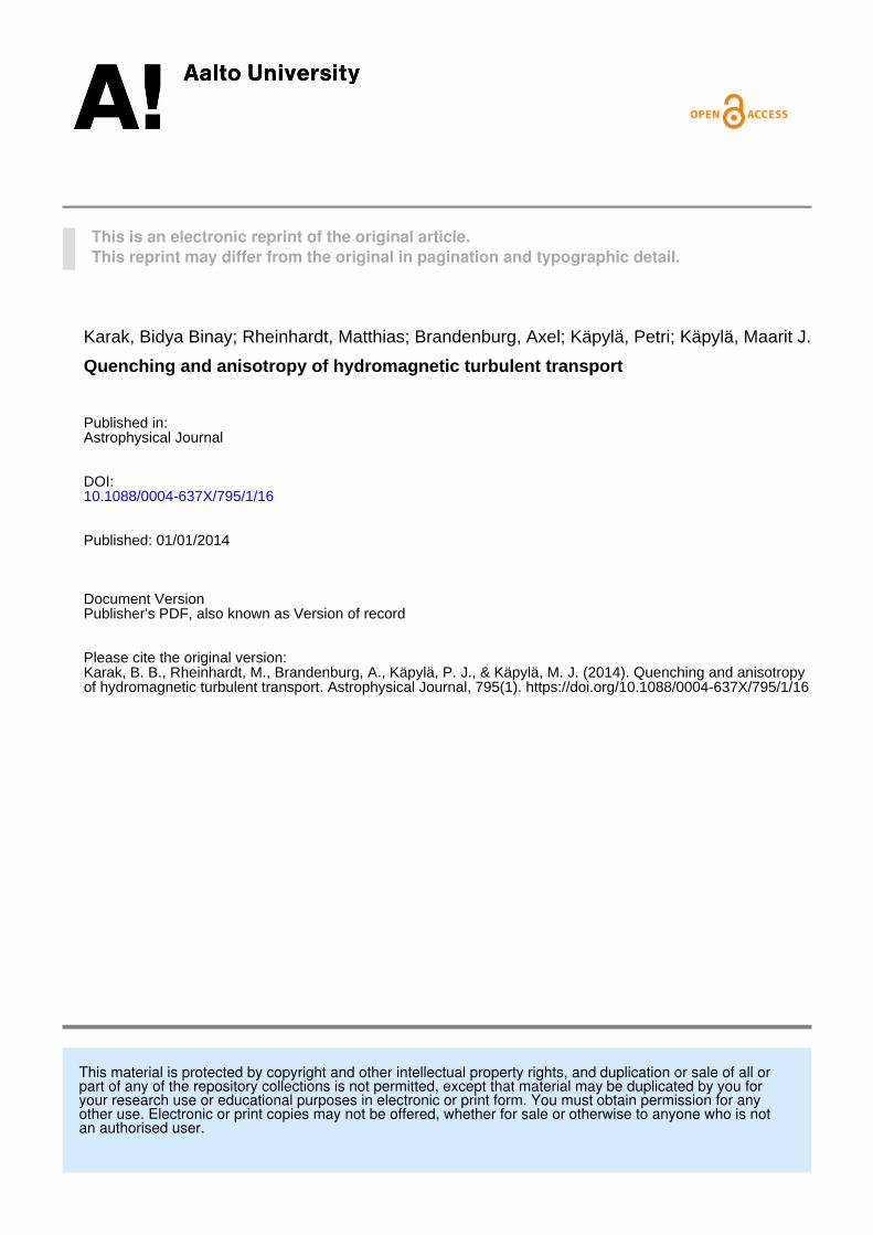
Figure 2. Dependence of η11 and η22 on the imposed field for forced turbulence;Rm0 = 0.87. Left: Set TBx with Bext ‖ x; right: Set TBz with Bext ‖ z.Dashed lines: fits from Equation (32) with exponents qη; dotted lines: fits fromEquation (34).
(A color version of this figure is available in the online journal.)
interest; see Section 4.2.4. As expected, and in agreement withearlier work (Brandenburg et al. 2012), γ and δ also vanish onaverage and are not shown here.
The time spans for temporal averaging should ideally be solong that the averages become stationary. How close we cameto this is in several cases indicated by error bars showing thelargest deviation of the average over any one-third of the timeseries from the overall average.
It is convenient to normalize the results using the unquenchedand hence isotropic expression for ηt as obtained in SOCA inthe high conductivity limit, i.e.,
ηt0 = 13urms0k
−1f . (33)
When we determine the fluctuations of α, we use α0 = urms0/3for normalization, which would be the expected value in fullyhelically forced isotropic turbulence. First, we present thetransport coefficients measured using TFZ, but restrict ourselvesto η11 and η22.
4.2.1. TFZ: Horizontal and Vertical Fields
Figure 2 shows the results for both horizontal and verticalexternal fields, Bext = Bext x (Set TBx) and Bext = Bext z (SetTBz); see Table 1. For these runs we have adopted kf /k1 = 5and η = ν = 0.01 cs/k1, which yields Rm0 = 0.87. Notethat in both cases η11 is almost identical to η22, which isnatural for the vertical field, but unexpected for the horizontalone, because ηij , being an axisymmetric rank-2 tensor whose
preferred direction is given by B ‖ Bext, must have the general
form ηij = η0δij +η1BiBj with B-dependent coefficients η0 andη1. This has indeed been confirmed previously for a dynamo-generated B of Beltrami type (Brandenburg et al. 2008b). Forhorizontal Bext we have thus η11 = η0 + η1, but η22 = η0. Thereason for the apparent vanishing of η1 is currently unclear,but might be connected with the fact that here the field is auniform one.
Indeed, considering a forcing, simplified such that only asingle transverse (frozen) wave is supported instead of switchingrapidly between waves with random wavevector and phase,one finds that a uniform imposed field of arbitrary strengthdoes not change the geometry of that wave, but merely itsamplitude, see the Appendix. Hence, for a statistical ensemble,generated by random choices of wave and polarization vectors,ηij from averaging over this ensemble must remain isotropic,that is, η1 needs to vanish. The only condition for that tohold is the negligibility of the pressure variations caused bythe imposed field, compared to the pressure in the field-free
case. This finding looks similar to that obtained for the Robertsforcing case, although the mathematical reason is here thetransversality of the wave flow and not its Beltrami property.Returning to the actually used delta-correlated random-waveforcing, one would conclude, that approximate isotropy couldoccur as long as the waves are damped quickly enough forletting their mutual interactions be subdominant. Of course, ifat all, this can only happen for small Re and Rm as those in SetsTBx and TBz (Re0 = Rm0 = 0.87). With increasing Reynoldsnumbers, anisotropy should gradually emerge, and indeed, forRe0 = Rm0 ≈ 14 we find η11 being by ≈9% bigger than η22when the imposed field is as weak as Bext/Beq = 0.66.
Unlike the Roberts flow case, the behavior for Bext > Beqcannot be described by a single asymptotic power law. Insteadwe observe a possible transition from one power law to anotherone with lower power at Bext � 20Beq. Accordingly, the fittingformula (32), with quenching exponents qη = 1.1 for both casesmatches well only up to this value. Nevertheless in Figure 2 wesee that the quenching is not exactly the same for the two fielddirections, namely, slightly weaker for the vertical field as wefind pη = 0.21 for the latter, but pη = 0.38 for the horizontalfield.
A satisfactory overall fit can be obtained by employing anansatz of the form
η11,22(Bext) = η11,22(0)1 + pn(Bext/Beq)q
1 + pd (Bext/Beq)q(34)
with q = 1.36 and 1.31 for horizontal and vertical field,respectively; see the red dotted lines in Figure 2. This can betaken as an indication of asymptotic independence of η11,22 onBext, which makes sense as the turbulence should asymptoticallybecome two-dimensional with Bext · ∇u = 0. Note that we donot observe this in the Roberts forcing case because there, asdemonstrated above, the flow has no freedom to adjust to thiscondition, at least for not too high Rm.
If we normalize Bext in Equation (32) by Beq0, the scalingchanges and the exponent qη becomes 1.5 and 1.4 for horizontaland vertical external fields, respectively. These values are higherthan the result of Kitchatinov et al. (1994) and Rogachevskii &Kleeorin (2001), who found unity.
When comparing the two panels of Figure 2 one might askwhy the quenching characteristics of η22 for horizontal andvertical Bext are not identical although this coefficient is inboth cases correlating components of E and J perpendicular tothe preferred direction. This apparent ambiguity can be resolvedwith a view to Equation (5): Provided that ε ≈ 0 (which will bedemonstrated in the next section), we have for vertical externalfield ∇ = ∇‖ ez, hence ηt and μ sum up, while for horizontalBext of course ∇‖ = 0, so η11(= η22) should differ in the twocases roughly by μ. That is, the anisotropy of the turbulencedoes manifest in the diffusive behavior, but not by causing ananisotropic ηij .
4.2.2. TFA: Determining Anisotropy
To measure the anisotropy of turbulent diffusion, we haveapplied TFA for axisymmetric turbulence whose preferreddirection is defined by the imposed field. Hence, we considerthe case Bext = Bext z. We measure all the relevant transportcoefficients described in Equation (4). Here we only show η⊥,η‖, and μ. It turns out that κ⊥ and κ‖ are negative (around −0.01in units of ηt0) for our largest field strengths, but zero withinerror bars for weaker fields and hence not shown. All other
8
The Astrophysical Journal, 795:16 (16pp), 2014 November 1 Karak et al.
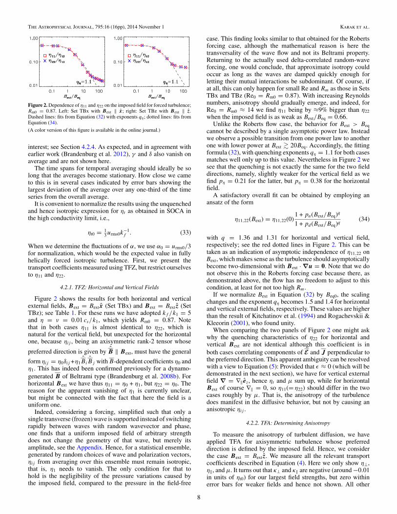
Figure 3. Results of Set AT1, Rm0 = 2.23. Variation of η‖ (crosses), η⊥(triangles), μ (diamonds, dotted), and η⊥ − μ/2 (squares), all normalized byηt0, with the imposed field Bext/Beq; dashed and dash-dotted: fits to η‖ and η⊥,respectively, from Equation (32). Dashed line in inset: linear fit with slope 0.2.
(A color version of this figure is available in the online journal.)
Figure 4. As Figure 3, but for Set AT2, Rm0 = 18.2 and the linear fit (dashedline in inset) has slope 0.6 here.
(A color version of this figure is available in the online journal.)
coefficients are at least about 10 times smaller and fluctuatingabout zero; see Section 4.2.4 for some discussion about thosefluctuations. We denote this set of simulations by AT1 and showits results in Figure 3; see also Table 1. It turns out that η⊥ is lessstrongly quenched than η‖. According to the fitting formula (32),we have q‖ = 1.2, but q⊥ = 0.85. The coefficient μ is increasingwith Bext until a maximum at Bext/Beq ≈ 2. Interestingly,we have η‖ ≈ η⊥ − μ/2; see red squares in Figure 3. Ifwe apply this finding in Equation (5) we see that because ofε ≈ 0 the mean-field induction equation takes the simple form∂t B = (
(η + η⊥ − μ/2)∇2 + μ∇2‖)B. We may redefine the
preferred direction to coincide now with x and assume at thesame time, that all mean quantities depend solely on z, hence∇‖ = 0. In this way we can make contact with the results ofTFZ for horizontal fields arriving at η11 = η22 = η⊥ − μ/2. So
Figure 5. Rm dependence of the turbulent diffusivity in axisymmetric turbulencewith a fixed Bext/Beq ≈ 4.3 (Set AT3). Squares: η⊥−μ/2; crosses: η‖; trianglesη⊥; diamonds: μ, all normalized by ηt0.
(A color version of this figure is available in the online journal.)
Figure 6. Small portion of the time series of z-averaged η⊥ and η‖ for thehighest Rm = 537 (from Set AT3) with imposed field Bext/Beq ≈ 4.3. Timeis normalized by the turnover time (urmskf )−1. Dashed lines: averages over theresetting intervals. We take the average of many (�10) such intervals.
(A color version of this figure is available in the online journal.)
the somewhat surprising isotropy of ηij obtained with TFZ isconfirmed with TFA in spite of η⊥ �= η‖.
4.2.3. Rm Dependence
To study the influence of Rm, we performed simulations withthe higher value Rm0 = 18.2; see Set AT2 in Table 1. Figure 4shows that for this set the quenching exponents of η⊥ and η‖are reduced mildly. The μ increases more rapidly with Bextcompared to Set AT1 and seems to saturate at large fields.Moreover, we have performed simulations with a fixed valueof Bext/Beq ≈ 4.3, but Rm increasing from 0.07 to 537; seeFigure 5. For the largest values of Rm, the resetting of the testsolutions (see Section 3.4) is most critical, but it turns out thatthe resulting values of η⊥ and η‖ show clear plateaus wherestatistically stable averages can be taken; see Figure 6 for anexample.
At low Rm we do not see much anisotropy, but for Rm > 1,η⊥ becomes significantly larger than η‖. Interestingly, at aboutRm = 10, η‖ reaches a maximum, whereas η⊥ increases even atthe largest Rm, as does μ. We find again that η⊥ −μ/2 is almostidentical to η‖.
It has been reported earlier that in forced hydrodynamicturbulence ηt increases linearly with Rm at smaller values andsaturates beyond Rm ≈ 10 (Sur et al. 2008). However this
9

The Astrophysical Journal, 795:16 (16pp), 2014 November 1 Karak et al.
Figure 7. As Figure 5, but showing the fluctuations of α as functions of Rm.Crosses: αrms
‖ ; triangles: αrms⊥ .
(A color version of this figure is available in the online journal.)
is not so in our hydromagnetic turbulence. Unfortunately, theinstability of the test problems for high Rm prevents us fromlooking further for a possible saturation.
4.2.4. Incoherent α Effect
For non-helical isotropic forcing, the α tensor vanishes onaverage when rotation or stratification is absent. As emphasizedby Brandenburg et al. (2008a), however, its fluctuations, alsoreferred to as “incoherent α effect,” may in general haverelevance for dynamo processes, especially if they interact withlarge-scale shear (Vishniac & Brandenburg 1997; Heinemannet al. 2011; Mitra & Brandenburg 2012). In our simulationsthey are too weak to lead to self-excitation though. In Figure 7we show the volume-averaged temporal fluctuations of α⊥ andα‖ as functions of Rm in terms of their rms values, defined as〈α2
⊥〉1/2t and 〈α2
‖〉1/2t , respectively, where the subscript t refers to
time averaging. While αrms⊥ increases with Rm, αrms
‖ increasesonly slightly at moderate Rm, but decreases beyond Rm ≈ 5.Fluctuations in z could also be important and would increasethe rms values of α⊥ and α‖ but have been ignored here.
4.3. Stratified Convection
Finally, we turn to convection, in which already in the absenceof a magnetic field a preferred direction is set by gravity and thusdensity stratification. All the relevant transport coefficients aremeasured using TFZ with wavenumber k = k1, except that inone case we also consider k = 0. As in the case of homogeneousforced turbulence, we present time-averaged results, but owingto the intrinsic inhomogeneity of the setup, no z averaging isperformed by default. Error bars are generated as described forforced turbulence.
In deriving quenching characteristics for an inhomogeneousturbulence from numerical experiments with an imposed (uni-form) field, one has to remember that the actually quenchingmean field needs not coincide with the imposed one. In general,as a consequence of Equation (1), a mean electromotive forceis caused by Bext, which in turn can give rise to an additionalconstituent of B. This could of course not happen in our setupswith forcing, as there the generated E is uniform. For convection,however, the transport coefficients are at least z dependent (forTFZ) and the x and y components of E will result in B �= Bextdue to the generation of one or even two components orthogonalto Bext. For horizontal Bext the imposed component itself is alsomodified.
Figure 8. Dependences of γ (left) and ηt (right) on the vertical coordinatez for different Bext/Beq (Set CR0). Hatched areas: errors (not shown forBext/Beq = 16.8 as indistinguishable from the mean). Dotted lines at z = 0, 1:boundaries of the convectively unstable region.
(A color version of this figure is available in the online journal.)
4.3.1. Non-rotating Convection
First, we present results for the simplest situation withoutrotation or large-scale shear (Set CR0, listed in Table 1). No(coherent) α effect is expected, but turbulent pumping, i.e., aγ effect, should occur due to the inhomogeneities caused bystratification and boundaries. Figure 8 presents profiles of γand ηt for four different values of the imposed magnetic fieldBext from zero to ≈17Beq. We see that the unquenched profilesof γ and ηt are similar to what has been found by Kapylaet al. (2009a) and that even when Bext/Beq � 1, at least ηt isnot quenched much. However, for Bext/Beq > 2, both γ andηt are suppressed significantly, and γ is even changing sign.Moreover, the level of fluctuations is markedly reduced at thehighest Bext/Beq and the convection itself is suppressed to theextent that it only shows elongated cells; see Table 1 for thereduction of urms (cf. Rm). This is a consequence of our choiceof using relatively small values of Rm and Re, with the effectthat the convection is only mildly supercritical and thereforemore vulnerable to quenching.
For weak and moderately strong fields, negative (positive)values of γ are seen in the upper (lower) part of the domain,which corresponds to downward (upward) pumping, i.e., towardthe middle of the convection zone. These directions are justopposite to what analytic theory predicts for uniform meanfields, namely, that the pumping is directed away from themaximum of the turbulence intensity. The obtained behavioragrees, however, with the findings of Kapyla et al. (2009a) forharmonic test fields with k = k1 which are also employed in thissection. For stronger fields the sign is reversed, as expected formagnetic buoyancy (Kitchatinov & Pipin 1993). In Section 4.3.3we will show results for uniform test fields (k = 0) and comparethem with the theoretical prediction.
The coefficients are intrinsically z dependent, but for thesake of clarity in presenting their dependences on Bext, wecalculate the averages of η11,22 and |γ | over a certain z extent,typically 0.2 � z/d � 0.9. Other intervals or even thedegenerate case of fixed values of z, however, yield very similarquenching behaviors. In Figure 9, we present η11,22 and γ ,averaged in this way, in dependence on Bext. Fitting the datawith the formula (32), we find qγ,η = 1.2, which is veryclose to our earlier results for the Roberts flow, but slightlylarger than those found in forced turbulence. Finding the samequenching dependence of γ and ηt seems sensible in light ofthe result of the linear theory of Roberts & Soward (1975),γ = −∂zηt/2. When we normalize Bext with Beq0 we find forthe exponents qγ,η ≈ 2.2. The value of qγ disagrees with the
10

The Astrophysical Journal, 795:16 (16pp), 2014 November 1 Karak et al.
Figure 9. Results from Set CR0: Dependences of 〈η11〉z (squares) 〈η22〉z(crosses) and 〈|γ |〉z (diamonds) on Bext/Beq. Dashed lines: fits fromformula (32) with exponents qη,γ = 1.2.
(A color version of this figure is available in the online journal.)
analytical result of Rogachevskii & Kleeorin (2006). However,this was derived for turbulent pumping being caused by thedensity gradient, which can hardly be dominant here because ofweak density stratification. Therefore, our result is closer to theexponent 2 that is found when pumping is caused by a gradientin the turbulence intensity instead (see Section 4.3.3 for thevalidation).
4.3.2. Rotating Convection
Next we consider rotating convection with the rotation axisaligned along the z direction (θ = 0), whereas the magneticfield is along the x direction. We expect an α-effect becauseg · Ω �= 0. Figure 10 shows the profiles of the measuredtransport coefficients at different strengths of the external fieldwith αij normalized to the isotropic value for maximum helicityα0 = urms0/3 and ηij normalized to ηt0 (see Eq. (33)). The maindiagonal elements of both tensors are for Bext �= 0 not equalbecause the external field is applied along the x direction. Forvanishing and weak Bext, both α11 and α22 change sign, albeit notat exactly the same position; they are then positive in (roughly)the upper half of the convective zone and negative in the lowerone, again consistent with earlier findings of Ossendrijver et al.(2001) and Kapyla et al. (2009a). Importantly, α11 decreasesrapidly with increasing Bext. However, α22 increases at first andonly later decreases.
The components η11,22 have very similar profiles not onlyfor vanishing, but also for very strong magnetic field, differinga bit more for intermediate field strengths. The off-diagonalcomponents of the η tensor are here of interest mainly in thecombination δ = (η21 − η12)/2, which characterizes the Ω × Jeffect. In agreement with earlier work for rotating convection(Kapyla et al. 2009a), the sign of δ is mainly positive, whilefor rotating forced turbulence, Brandenburg et al. (2008a, 2012)found it to be negative. It is also remarkable that δ is onlymildly quenched unless the magnetic field becomes very strong.We further see that η21 + η12 is not small. This quantity wouldvanish in the absence of a magnetic field, but it is apparentlyquite sensitive even to weak fields.
The lowermost panels in Figure 10 show the mean kinetic andcurrent helicity as defined by hk = ω · u with ω = ∇ × u, andhc = j · b, respectively. For weak fields, the kinetic helicityis positive in the lower third and negative in the upper twothirds of the unstable layer, while the current helicity changes
Figure 10. Results from Set CR1: variations of αij , ηij , γ , δ, and the mean kineticand current helicity, hk and hc , respectively, along the vertical coordinate z atdifferent field strengths. hk and hc are normalized by 〈u2〉V kf and ρ〈u2〉V kf ,respectively, where 〈·〉V indicates volume averaging. Dotted lines at z/d = 0, 1:boundaries of the convectively unstable region.
(A color version of this figure is available in the online journal.)
from positive to negative only at z ≈ 0.6d. So the expectationof sign equality of the helicities, nourished by ideas of αquenching originating from closure approaches (Pouquet et al.1976; Kleeorin & Ruzmaikin 1982), is only very roughly met.For strong fields, however, both helicities show only one sign,opposite to each other, over almost the entire domain. Thecurrent helicity increases first rapidly with the imposed field,but for the strongest fields both helicities begin to be quenched.
In Figure 11, showing the absolute values of the transportcoefficients averaged over 0.2 � z/d � 0.9, we find 〈|α11|〉zbeing quenched according to Equation (32) with qα11 = 1.8. Bycontrast, 〈|α22|〉z is growing until Bext/Beq ≈ 6, where it reachesroughly eight times its unquenched value, and is falling then, butwith a lower power than 〈|α11|〉z, namely, qα22 ≈ 1. Similarly tothe α quenching for Roberts forcing, we find that the quenchingexponents are larger when normalizing by Beq0: about 3 for〈|α11|〉z and asymptotically perhaps about 2 for 〈|α22|〉z. Thepower 3 agrees with earlier analytic results of Moffatt (1972),Rudiger (1974), and Rudiger & Kitchatinov (1993), while the
11

The Astrophysical Journal, 795:16 (16pp), 2014 November 1 Karak et al.
Figure 11. Results from Set CR1: variations of (a) 〈|α11,22|〉z, (b) 〈|α12,21|〉z,〈|γ ]〉z, (c) 〈η11,22〉z, and (d) 〈|δ|〉z with the external field. Dashed lines: fits fromEquation (32).
(A color version of this figure is available in the online journal.)
power 2 agrees with the exponent found by Rogachevskii &Kleeorin (2000), who all normalized by Beq0.
The quantities 〈ηt 〉z and 〈|γ |〉z show also systematic quench-ing with exponents very similar to those found earlier in non-rotating convection (q = 1.2) and in fact identical to the resultsfor Roberts forcing (q = 1.3). As we have rotation, another rel-evant quantity is δ, defined in Equation (24), which is essentialfor the Ω × J dynamo in non-helical turbulence with shear, cf.Equation (4). For a recent application to stellar dynamos seePipin & Seehafer (2009). Figure 11 shows the variation of 〈|δ|〉zwith Bext, and we find strong quenching with qδ = 2.
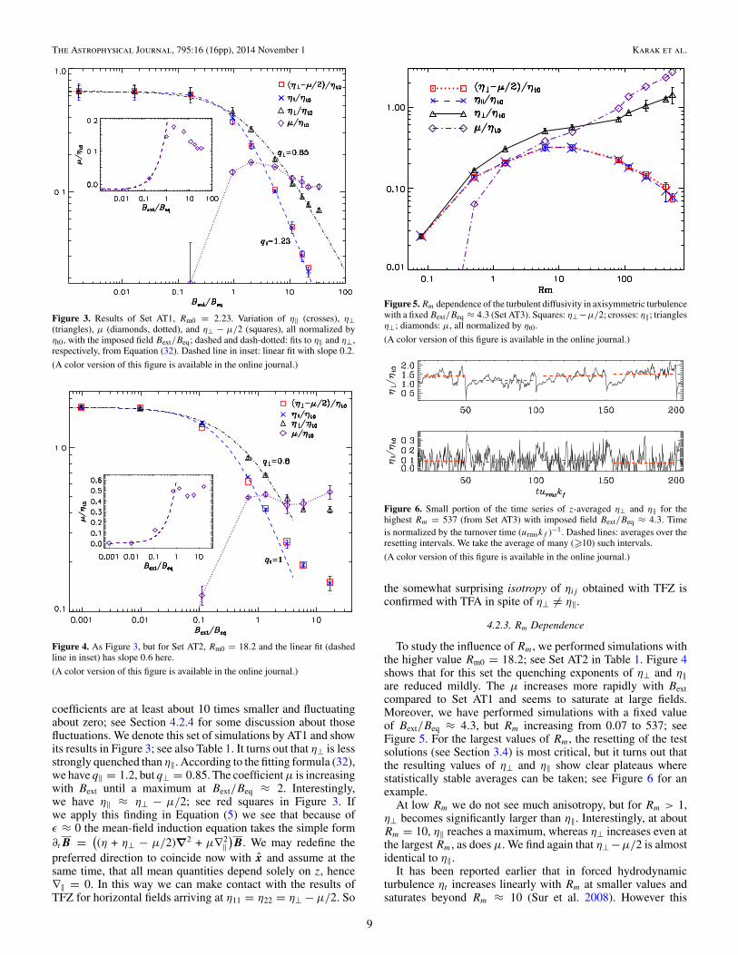
As mentioned above, for the inhomogeneous turbulence inconvection we must take into account that B �= Bext. Therefore,we show in Figure 12 for Set CR1 (cf. Figure 11), how thetransport coefficients are quenched with the local B(z)/Beq(z).For comparison, the fit to the z averaged quantities fromEquation (32) is shown by the dashed lines. A more appropriaterepresentation is obtained by considering the turbulent transportcoefficients as functions of both the local B(z) and Rm0(z), asthey should also depend on the intrinsic (unquenched) localstrength of the turbulence. This view is provided in Figure 13,where the arguments in the (B/Beq, Rm0) plane were formedby taking both quantities from the same set of z positionswithin the convection zone for eight different values of Bext. Theshown surface was then obtained by linear interpolation over aDelaunay triangulation of the irregularly spaced arguments. Inη11,22 we see for fixed Rm0 the common power-law quenchingbehavior, while the dependence on Rm0 for fixed B/Beq growsuntil saturation for small B/Beq � 5, but falling beyond. |α11|shows a similar power-law behavior with B/Beq for fixed Rm0,but there is in general a sign change of α11 for B/Beq between1 and 10. At best, a very narrow Rm0 interval exists withoutsign change. As already indicated by Figure 11, the behavior of|α22| is different in that it is first growing with B/Beq reaching amaximum at ≈5 for all values of Rm0. As a remarkable featurewe see a sign change only up to B/Beq � 3. Beyond, the Rm0dependence is becoming weak with a flat maximum.
It remains open, whether the transport coefficients are re-ally local functions of the two quantities employed, or whetherthere is also a generic dependence on the local mean cur-rent density. In addition, non-locality of turbulent transport has
Figure 12. As Figure 11 from Set CR1, but all coefficients are computed locallyat 14 equidistant z positions, 0.2 d � z � 0.9 d, in the convective zone andare plotted against the local value of B(z)/Beq(z). Each curve, limited by filledand open circles, corresponds to one of the values of Bext/〈Beq0(z)〉z out of0.21, 0.83, 2.1, 4.1, 10.3, 20.7, 31.0, and 41.3, in the order of increasing B/Beq-positions of filled circles (but not necessarily of open circles). Filled and opencircles refer to z/d = 0.2 and z/d = 0.9, respectively, thus z is the curveparameter. Dashed lines: fits to the z averaged quantities from Equation (32).Red/dash-dotted curve sections in (b), (c), and (d) indicate negative γ , α11,22and δ.
(A color version of this figure is available in the online journal.)
been ignored throughout, which is only permissible at largeenough scale separation; see Rheinhardt & Brandenburg (2012).Note that the dependences on B/Beq and Rm0 were entan-gled in the result of Brandenburg et al. (2008b) as there B,being dynamo generated, could not be varied independentlyof Rm0.
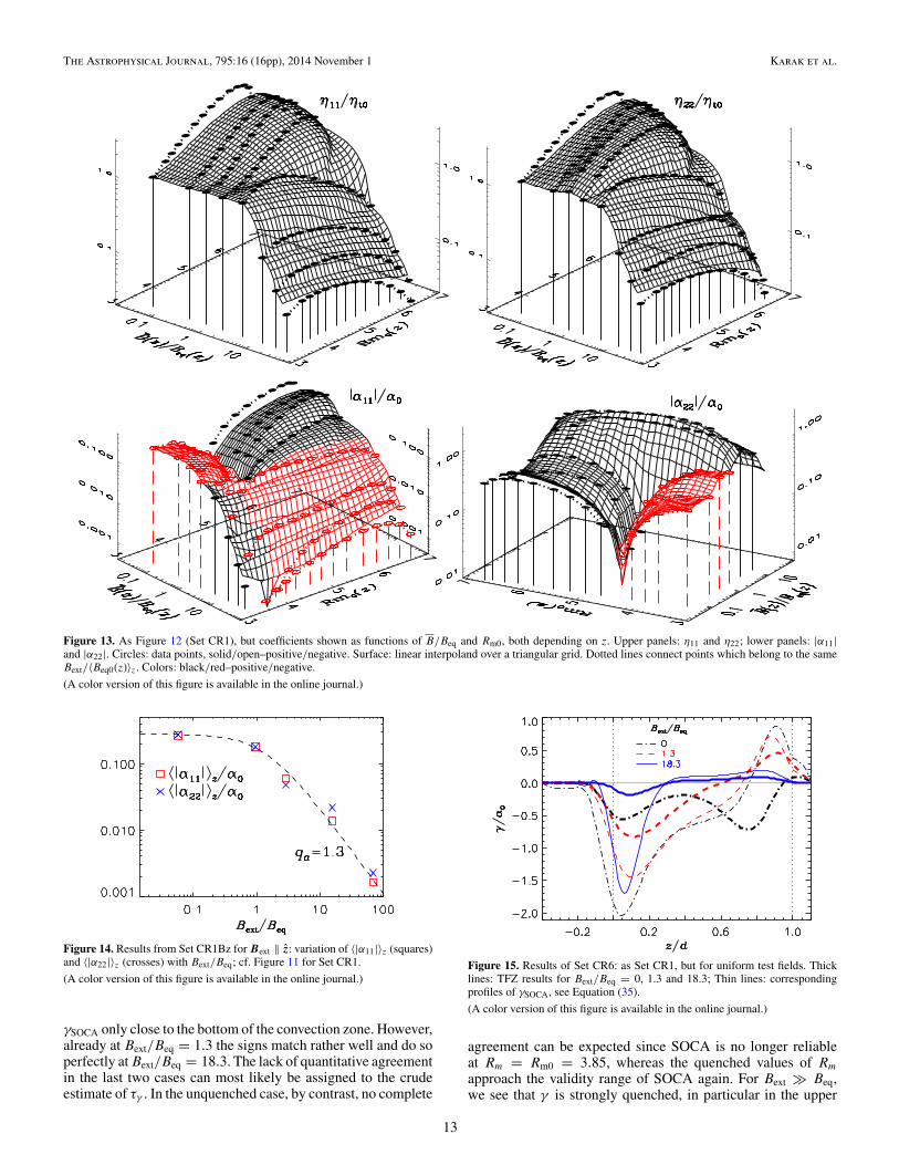
In another set of simulations, the external field is applied alongthe vertical direction; see Set CR1Bz in Table 1. Figure 14 showsthe dependences of 〈|α11,22|〉z on the external field. We see that〈|α11|〉z is very close to 〈|α22|〉z, but now both are quenchedwith the exponent qα = 1.3, which is smaller than the one of〈|α11|〉z for horizontal external field; see Set CR1. Unlike inthat case, 〈|α22|〉z shows no “anti-quenching”; cf. Figure 11. For〈ηt 〉z and 〈|γ |〉z, the quenching exponents are equal to those forthe horizontal field case, but for 〈|δ|〉z we get qδ = 1.8 instead of2. To confirm these findings, we have repeated the simulationsat higher Ra and Rm and find similar results; see Set CR3Bz inTable 1.
4.3.3. Turbulent Pumping for Uniform Test Fields
According to analytic SOCA theory, developed for uniform(or linear) mean fields, turbulent pumping is related to theinhomogeneity of the turbulence through (Krause & Radler1980)
γSOCA = −(τγ /2)∂zu2z , τγ ≈ τ corr. (35)
Hence, we now employ TFZ with uniform test fields (k = 0)in the sets CR6 and CR7 having horizontal imposed field, seeTable 1. Figure 15 shows the z profiles of γ for different values ofBext together with those of γSOCA where τ corr has been set to the(z dependent) mixing-length estimate Hp/〈u2〉1/2
t . Comparisonreveals that for Bext = 0 there is sign agreement of γ and
12
The Astrophysical Journal, 795:16 (16pp), 2014 November 1 Karak et al.
Figure 13. As Figure 12 (Set CR1), but coefficients shown as functions of B/Beq and Rm0, both depending on z. Upper panels: η11 and η22; lower panels: |α11|and |α22|. Circles: data points, solid/open–positive/negative. Surface: linear interpoland over a triangular grid. Dotted lines connect points which belong to the sameBext/〈Beq0(z)〉z. Colors: black/red–positive/negative.
(A color version of this figure is available in the online journal.)
Figure 14. Results from Set CR1Bz for Bext ‖ z: variation of 〈|α11|〉z (squares)and 〈|α22|〉z (crosses) with Bext/Beq; cf. Figure 11 for Set CR1.
(A color version of this figure is available in the online journal.)
γSOCA only close to the bottom of the convection zone. However,already at Bext/Beq = 1.3 the signs match rather well and do soperfectly at Bext/Beq = 18.3. The lack of quantitative agreementin the last two cases can most likely be assigned to the crudeestimate of τγ . In the unquenched case, by contrast, no complete
Figure 15. Results of Set CR6: as Set CR1, but for uniform test fields. Thicklines: TFZ results for Bext/Beq = 0, 1.3 and 18.3; Thin lines: correspondingprofiles of γSOCA, see Equation (35).
(A color version of this figure is available in the online journal.)
agreement can be expected since SOCA is no longer reliableat Rm = Rm0 = 3.85, whereas the quenched values of Rm
approach the validity range of SOCA again. For Bext � Beq,we see that γ is strongly quenched, in particular in the upper
13
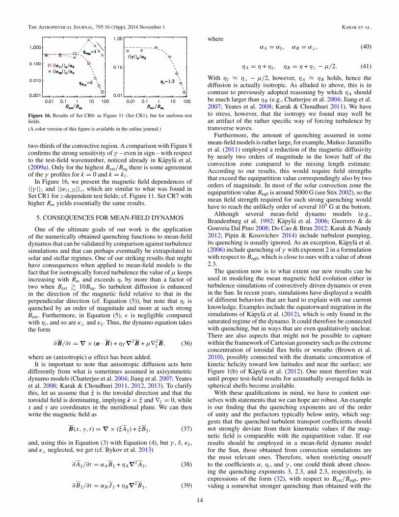
The Astrophysical Journal, 795:16 (16pp), 2014 November 1 Karak et al.
Figure 16. Results of Set CR6: as Figure 11 (Set CR1), but for uniform testfields.
(A color version of this figure is available in the online journal.)
two-thirds of the convective region. A comparison with Figure 8confirms the strong sensitivity of γ – even in sign – with respectto the test-field wavenumber, noticed already in Kapyla et al.(2009a). Only for the highest Bext/Beq there is some agreementof the γ profiles for k = 0 and k = k1.
In Figure 16, we present the magnetic field dependences of〈|γ |〉z and 〈|α11,22|〉z, which are similar to what was found inSet CR1 for z-dependent test fields; cf. Figure 11. Set CR7 withhigher Rm yields essentially the same results.
5. CONSEQUENCES FOR MEAN-FIELD DYNAMOS
One of the ultimate goals of our work is the applicationof the numerically obtained quenching functions to mean-fielddynamos that can be validated by comparison against turbulencesimulations and that can perhaps eventually be extrapolated tosolar and stellar regimes. One of our striking results that mighthave consequences when applied to mean-field models is thefact that for isotropically forced turbulence the value of μ keepsincreasing with Rm and exceeds ηt by more than a factor oftwo when Bext � 10Beq. So turbulent diffusion is enhancedin the direction of the magnetic field relative to that in theperpendicular direction (cf. Equation (5)), but note that ηt isquenched by an order of magnitude and more at such strongBext. Furthermore, in Equation (5), ε is negligible comparedwith ηt , and so are κ⊥ and κ‖. Thus, the dynamo equation takesthe form
∂ B/∂t = ∇ × (α · B) + ηT ∇2 B + μ∇2‖ B, (36)
where an (anisotropic) α effect has been added.It is important to note that anisotropic diffusion acts here
differently from what is sometimes assumed in axisymmetricdynamo models (Chatterjee et al. 2004; Jiang et al. 2007; Yeateset al. 2008; Karak & Choudhuri 2011, 2012, 2013). To clarifythis, let us assume that z is the toroidal direction and that thetoroidal field is dominating, implying e = z and ∇‖ = 0, whilex and y are coordinates in the meridional plane. We can thenwrite the magnetic field as
B(x, y, t) = ∇ × ( zA‖) + zB‖, (37)
and, using this in Equation (3) with Equation (4), but γ , δ, κ‖,and κ⊥ neglected, we get (cf. Bykov et al. 2013)
∂A‖/∂t = αAB‖ + ηA∇2A‖, (38)
∂B‖/∂t = αBJ ‖ + ηB∇2B‖, (39)
whereαA = α‖, αB = α⊥, (40)
ηA = η + η‖, ηB = η + η⊥ − μ/2. (41)
With η‖ ≈ η⊥ − μ/2, however, ηA ≈ ηB holds, hence thediffusion is actually isotropic. As alluded to above, this is incontrast to previously adopted reasoning by which ηA shouldbe much larger than ηB (e.g., Chatterjee et al. 2004; Jiang et al.2007; Yeates et al. 2008; Karak & Choudhuri 2011). We haveto stress, however, that the isotropy we found may well bean artifact of the rather specific way of forcing turbulence bytransverse waves.
Furthermore, the amount of quenching assumed in somemean-field models is rather large, for example, Munoz-Jaramilloet al. (2011) employed a reduction of the magnetic diffusivityby nearly two orders of magnitude in the lower half of theconvection zone compared to the mixing length estimate.According to our results, this would require field strengthsthat exceed the equipartition value correspondingly also by twoorders of magnitude. In most of the solar convection zone theequipartition value Beq0 is around 5000 G (see Stix 2002), so themean field strength required for such strong quenching wouldhave to reach the unlikely order of several 105 G at the bottom.
Although several mean-field dynamo models (e.g.,Brandenburg et al. 1992; Kapyla et al. 2006; Guerrero & deGouveia Dal Pino 2008; Do Cao & Brun 2012; Karak & Nandy2012; Pipin & Kosovichev 2014) include turbulent pumping,its quenching is usually ignored. As an exception, Kapyla et al.(2006) include quenching of γ with exponent 2 in a formulationwith respect to Beq0, which is close to ours with a value of about2.3.
The question now is to what extent our new results can beused in modeling the mean magnetic field evolution either inturbulence simulations of convectively driven dynamos or evenin the Sun. In recent years, simulations have displayed a wealthof different behaviors that are hard to explain with our currentknowledge. Examples include the equatorward migration in thesimulations of Kapyla et al. (2012), which is only found in thesaturated regime of the dynamo. It could therefore be connectedwith quenching, but in ways that are even qualitatively unclear.There are also aspects that might not be possible to capturewithin the framework of Cartesian geometry such as the extremeconcentration of toroidal flux belts or wreaths (Brown et al.2010), possibly connected with the dramatic concentration ofkinetic helicity toward low latitudes and near the surface; seeFigure 1(b) of Kapyla et al. (2012). One must therefore waituntil proper test-field results for azimuthally averaged fields inspherical shells become available.
With these qualifications in mind, we have to content our-selves with statements that we can hope are robust. An exampleis our finding that the quenching exponents are of the orderof unity and the prefactors typically below unity, which sug-gests that the quenched turbulent transport coefficients shouldnot strongly deviate from their kinematic values if the mag-netic field is comparable with the equipartition value. If ourresults should be employed in a mean-field dynamo modelfor the Sun, those obtained from convection simulations arethe most relevant ones. Therefore, when restricting oneselfto the coefficients α, ηt , and γ , one could think about choos-ing the quenching exponents 3, 2.3, and 2.3, respectively, inexpressions of the form (32), with respect to Bext/Beq0, pro-viding a somewhat stronger quenching than obtained with the
14

The Astrophysical Journal, 795:16 (16pp), 2014 November 1 Karak et al.
usually adopted exponent 2. However, given that dynamo fieldsare non-uniform, more elaborated models for the dependence ofthe transport coefficients on both the local B and the local Beq0,perhaps even also including a dependence on the local J , needto be developed.
6. CONCLUSIONS
We have measured the quenching of the turbulent transportcoefficients appearing in the mean-field dynamo equation, inparticular αij , γ , ηij , δ, and μ, by test-field methods. Forthis, we have considered three different background flows onwhich uniform external magnetic fields with various directionswere imposed. This is of course quite different from the realsituation where quenching occurs due to dynamo-generatedmean fields; see Brandenburg et al. (2008b) for a measurementof α and ηt at large values of Rm in such a case. Anotheraspect to keep in mind is that the magnetic and fluid Reynoldsnumbers of our simulations are far too small in comparison withastrophysical situations. Extrapolation to Rm → ∞ is feasibleonce an asymptotic regime is detected, but we emphasize that,in agreement with the results of Brandenburg et al. (2008b), ourmaximum value of Rm � 600 is not yet sufficient. Nevertheless,the obtained results indicate clear trends that may well apply tomore realistic settings and parameter regimes.
In the setup with Roberts forcing, we have found as a strikingproperty of the quenching behavior its dependence on whetherone normalizes the external field with the actual or the original(unquenched) value of the equipartition field strength, Beq orBeq0, respectively. In the former case, the quenching exponentfor turbulent diffusivity and α effect is significantly smallerand closer to that found for forced turbulence and convection(around 1.3). In the latter case, on the other hand, we recover theexponent 4, found earlier for α quenching in the Roberts flow(Rheinhardt & Brandenburg 2010). Somewhat surprisingly, wefind the quenched αij and ηij to be still isotropic in the xy plane,in contrast to that paper. However, it is now clear that this is aconsequence of their use of a simplified momentum equationand that the obtained isotropy is physically sensible.
For isotropically forced turbulence, the differences betweenthe two normalizations of Bext are not so large and the exponentbased on Beq0 is only around 1.5, which is higher than whathas been found analytically in Kitchatinov et al. (1994) andRogachevskii & Kleeorin (2000), while the exponent based onBeq is around 1.1, which is similar to that found by Gressel et al.(2013).
Finally we have considered rotating stratified convection.Along with α and ηt , we have studied turbulent pumping (γ )and the Ω × J effect (δ). We find that ηt and γ show similarquenching dependences on Bext/Beq (with quenching exponentq ≈ 1.3), while q is about 2 for α and δ. However, when Bextis normalized with Beq0 the exponent becomes 3, which is inagreement with Rudiger & Kitchatinov (1993). In non-rotatingconvection, the quenching of γ and ηt is only slightly weakercompared to the rotating case.
We have not studied the simultaneous quenching of turbulenttransport by magnetic field and rotation, which is particularlyimportant in rapidly rotating stars. Furthermore, we have notyet applied TFA for convection, which is a subject of ourongoing work. It is unclear, however, how useful it wouldbe to consider quenching with this method, because only onepreferred direction is possible. More general methods would beneeded in the presence of a strong horizontal magnetic field.
We thank an anonymous referee for suggestions that improvedthe presentation. This work was supported in part by theEuropean Research Council under the AstroDyn ResearchProject No. 227952, and the Swedish Research Council GrantsNo. 621-2011-5076 and 2012-5797, as well as the ResearchCouncil of Norway under the FRINATEK grant 231444. Weacknowledge the allocation of computing resources providedby the Swedish National Allocations Committee at the Centerfor Parallel Computers at the Royal Institute of Technologyin Stockholm and the National Supercomputer Centers inLinkoping, the High Performance Computing Center North inUmeå, and the Nordic High Performance Computing Center inReykjavik.
APPENDIX
QUENCHING FOR A SINGLE WAVE FLOW
Assume the forcing in Equation (8) to be a single transverse(frozen) wave with time-dependent amplitude,
f = f (t) a cos ψ, ψ = k · x + φ,
a = k × e|k × e| , e � ‖ k − an arbitrary vector. (A1)
Then, in the absence of Bext
u(0) = a cos ψ
∫ t
−∞exp
(νk2(t ′ − t)
)f (t ′)dt ′ = u(0)(t) a cos ψ,
p(0) = const, ρ(0) = const, (A2)
is an exact solution of Equations (6) and (8) for arbitrary Re as,being a transverse wave, it obeys u(0) · ∇u(0) = 0, ∇ · u(0) = 0and ∇2u(0) = −k2u(0). Further,
b(1) = −Bextkx a sin ψ
∫ t
−∞exp
(ηk2(t ′ − t)
)u(0)(t ′)dt ′
= −β(1)(t)Bextkx a sin ψ (A3)
is an exact solution of the first-order induction equation withhorizontal Bext for arbitrary Rm, again as a consequence oftransversality and solenoidality of u(0). Likewise,
u(2) ≈ −B2extk
2x a cos ψ
∫ t
−∞exp
(νk2(t ′ − t)
)β(1)(t ′)dt ′/ρ(0),
p(2) ≈ −b(1)2/2 − b(1) · Bext, (A4)
is an approximate solution of the second-order momentumequation as long as p(2) � p(0), thus ρ ≈ ρ(0). As u(2) ∼ u(0)
(with a time-dependent factor) the argument continues to hold inarbitrary orders in Bext. The relation u(2) ∼ u(0) would even holdfor the less restricting condition that only the non-constant partof p(2) needs to be negligible. We conclude that the imposed fielddoes not change the geometry of the flow, but only its amplitude.Considering an ensemble of such flows with randomly chosen kand e, the transport coefficients obtained by ensemble averagingwould have to be isotropic, even when quenched, as long as thedensity remains close to uniform.
15
The Astrophysical Journal, 795:16 (16pp), 2014 November 1 Karak et al.
REFERENCES
Blackman, E. G., & Brandenburg, A. 2002, ApJ, 579, 359Braginsky, S. I. 1964, Ge&Ae, 4, 572Brandenburg, A. 2001, ApJ, 550, 824Brandenburg, A., Gressel, O., Kapyla, P. J., et al. 2013, ApJ, 762, 127Brandenburg, A., Jennings, R. L., Nordlund, Å., et al. 1996, JFM, 306, 325Brandenburg, A., Moss, D., & Tuominen, I. 1992, in ASP Conf. Ser. 27, The
Solar Cycle, ed. K. L. Harvey (San Francisco, CA: ASP), 536Brandenburg, A., Nordlund, Å., Pulkkinen, P., Stein, R. F., & Tuominen, I. 1990,
A&A, 232, 277Brandenburg, A., Radler, K.-H., & Kemel, K. 2012, A&A, 539, A35Brandenburg, A., Radler, K.-H., Rheinhardt, M., & Kapyla, P. J. 2008a, ApJ,
676, 740Brandenburg, A., Radler, K.-H., Rheinhardt, M., & Subramanian, K.
2008b, ApJL, 687, L49Brandenburg, A., Radler, K.-H., & Schrinner, M. 2008c, A&A, 482, 739Brown, B. P., Browning, M. K., Brun, A. S., Miesch, M. S., & Toomre, J.
2010, ApJ, 711, 424Brun, A. S., Miesch, M. S., & Toomre, J. 2004, ApJ, 614, 1073Bykov, A. M., Brandenburg, A., Malkov, M. A., & Osipov, S. M. 2013, SSRv,
178, 201Cattaneo, F., & Hughes, D. W. 1996, PhRvE, 54, R4532Cattaneo, F., & Vainshtein, S. I. 1991, ApJL, 376, L21Charbonneau, P. 2010, LRSP, 7, 3Chatterjee, P., Nandy, D., & Choudhuri, A. R. 2004, A&A, 427, 1019Choudhuri, A. R., & Gilman, P. A. 1987, ApJ, 316, 788Choudhuri, A. R., & Karak, B. B. 2009, RAA, 9, 953Choudhuri, A. R., & Karak, B. B. 2012, PhRvL, 109, 171103Covas, E., Tavakol, R., Tworkowski., A., & Brandenburg, A. 1998, A&A, 329,
350Del Sordo, F., Guerrero, G., & Brandenburg, A. 2013, MNRAS, 429, 1686Do Cao, O., & Brun, A. S. 2012, AN, 332, 907D’Silva, S., & Choudhuri, A. R. 1993, A&A, 272, 621Gilman, P. A. 1983, ApJS, 53, 243Gilman, P. A., & Miller, J. 1981, ApJ, 46, 211Glatzmaier, G. A. 1985, ApJ, 291, 300Gressel, O., Bendre, A., & Elstner, D. 2013, MNRAS, 429, 967Guerrero, G., & de Gouveia Dal Pino, E. M. 2008, ApJ, 485, 267Guerrero, G., Dikpati, M., & de Gouveia Dal Pino, E. M. 2009, ApJ, 701, 725Heinemann, T., McWilliams, J. C., & Schekochihin, A. A. 2011, PhRvL, 107,
255004Hubbard, A., & Brandenburg, A. 2009, ApJ, 706, 712Hubbard, A., Del Sordo, F., Kapyla, P. J., & Brandenburg, A. 2009, MNRAS,
398, 1891Hurlburt, N. E., Toomre, J., & Massaguer, J. M. 1986, ApJ, 311, 563Jepps, S. A. 1975, JFM, 67, 625Jiang, J., Chatterjee, P., & Choudhuri, A. R. 2007, MNRAS, 381, 1527Kapyla, P. J., & Brandenburg, A. 2009, ApJ, 699, 1059Kapyla, P. J., Korpi, M. J., & Brandenburg, A. 2008, A&A, 491, 353Kapyla, P. J., Korpi, M. J., & Brandenburg, A. 2009a, A&A, 500, 633Kapyla, P. J., Korpi, M. J., & Brandenburg, A. 2009b, ApJ, 697, 1153Kapyla, P. J., Korpi, M. J., & Tuominen, I. 2006, AN, 327, 884Kapyla, P. J., Mantere, M. J., & Brandenburg, A. 2012, ApJ, 755, 22Kapyla, P. J., Mantere, M. J., Cole, E., Warnecke, J., & Brandenburg, A.
2013, ApJ, 778, 41Karak, B. B. 2010, ApJ, 724, 1021Karak, B. B., & Choudhuri, A. R. 2011, MNRAS, 410, 1503
Karak, B. B., & Choudhuri, A. R. 2012, SoPh, 278, 137Karak, B. B., & Choudhuri, A. R. 2013, RAA, 13, 1339Karak, B. B, & Kapyla, P. J., Kapyla, M. J., & Brandenburg, A. 2014, A&A, in
press (arXiv:1407.0984)Karak, B. B, & Nandy, D. 2012, ApJL, 761, L13Kitchatinov, L. L., & Pipin, V. V. 1993, A&A, 274, 647Kitchatinov, L. L., Pipin, V. V., & Rudiger, G. 1994, AN, 315, 157Kleeorin, N., Moss, D., Rogachevskii, I., & Sokoloff, D. 2000, A&A, 361, L5Kleeorin, N. I., & Ruzmaikin, A. A. 1982, MHD, 18, 116Kohler, H. 1973, A&A, 25, 467Krause, F., & Radler, K.-H. 1980, Mean-Field Magnetohydrodynamics and
Dynamo Theory (Berlin: Akademie; Oxford: Pergamon)Mitra, D., & Brandenburg, A. 2012, MNRAS, 420, 2170Mitra, D., Kapyla, P. J., Tavakol, R., & Brandenburg, A. 2009, A&A, 495, 1Moffatt, H. K. 1972, JFM, 53, 385Munoz-Jaramillo, A., Nandy, D., & Martens, P. C. H. 2011, ApJL, 727, L23Ossendrijver, M., Stix, M., & Brandenburg, A. 2001, A&A, 376, 713Parker, E. N. 1955, ApJ, 122, 293Pipin, V. V., & Kosovichev, A. G. 2011, ApJL, 727, L45Pipin, V. V., & Kosovichev, A. G. 2014, ApJ, 785, 49Pipin, V. V., & Seehafer, N. 2009, A&A, 493, 819Pouquet, A., Frisch, U., & Leorat, J. 1976, JFM, 77, 321Racine, E., Charbonneau, P., Ghizaru, M., Bouchat, A., & Smolarkiewicz, P. K.
2011, ApJ, 735, 46Radler, K.-H. 2014, AN, 335, 459Radler, K.-H., Rheinhardt, M., Apstein, E., & Fuchs, H. 2002, MHD, 38, 41Rempel, M. 2006, ApJ, 647, 662Rheinhardt, M., & Brandenburg, A. 2010, A&A, 520, 28Rheinhardt, M., & Brandenburg, A. 2012, AN, 333, 71Rheinhardt, M., Devlen, E., Radler, K.-H., & Brandenburg, A. 2014, MNRAS,
441, 116Roberts, G. O. 1972, RSPTA, 271, 411Roberts, P. H., & Soward, A. M. 1975, AN, 296, 49Rogachevskii, I., & Kleeorin, N. 2000, PhRvE, 61, 5202Rogachevskii, I., & Kleeorin, N. 2001, PhRvE, 64, 056307Rogachevskii, I., & Kleeorin, N. 2003, PhRvE, 68, 036301Rogachevskii, I., & Kleeorin, N. 2006, GApFD, 100, 243Rogachevskii, I., Kleeorin, N., Brandenburg, A., & Eichler, D. 2012, ApJ,
753, 6Rudiger, G. 1974, AN, 295, 275Rudiger, G., & Brandenburg, A. 1995, A&A, 296, 557Rudiger, G., & Kitchatinov, L. L. 1993, AN, 269, 581Rudiger, G., & Kitchatinov, L. L. 2000, AN, 321, 75Rudiger, G., Kitchatinov, L. L., Kuker, M., & Schultz, M. 1994, GApFD, 78,
247Schrinner, M., Radler, K.-H., Schmitt, D., Rheinhardt, M., & Christensen, U.
2005, AN, 326, 245Schrinner, M., Radler, K.-H., Schmitt, D., Rheinhardt, M., & Christensen, U. R.
2007, GApFD, 101, 81Steenbeck, M., Krause, F., & Radler, K.-H. 1966, ZNatA, 21, 369Stix, M. 2002, The Sun: An Introduction (Berlin: Springer)Sur, S., Brandenburg, A., & Subramanian, K. 2008, MNRAS, 385, L15Sur, S., Subramanian, K., & Brandenburg, A. 2007, MNRAS, 376, 1238Vainshtein, S. I., & Cattaneo, F. 1992, ApJ, 393, 165Vishniac, E. T., & Brandenburg, A. 1997, ApJ, 475, 263Weber, M., Fan, Y., & Miesch, M. S. 2011, ApJ, 741, 11Yeates, A. R., Nandy, D., & Mackay, D. H. 2008, ApJ, 673, 544Yousef, T. A., Brandenburg, A., & Rudiger, G. 2003, A&A, 411, 321
16


![Tueurs de karak kadrin [8e edition]](https://img.dokumen.tips/doc/110x75/568c541b1a28ab4916bd7fcd/tueurs-de-karak-kadrin-8e-edition.jpg)