Embed Size (px)
Citation preview


Kandlikar I044527-Prelims.tex 31/10/2005 17: 30 Page i
HEAT TRANSFER AND FLUIDFLOW IN MINICHANNELSAND MICROCHANNELS

Kandlikar I044527-Prelims.tex 31/10/2005 17: 30 Page ii
Elsevier Internet Homepage
http://www.elsevier.com
Consult the Elsevier homepage for full catalogue information on all books, journals and electronic productsand services
Elsevier Titles of Related Interest
INGHAM AND POPTransport Phenomena in Porous Media III2005; ISBN: 0080444903www.elsevier.com/locate/isbn/0080449031
HARTNETT et al.Advances in Heat Transfer Volume 382004; ISBN: 0120200384www.elsevier.com/locate/isbn/0120200384
W. RODI AND M. MULASEngineering Turbulence Modelling and Experiments 62005; ISBN: 0080445446www.elsevier.com/locate/isbn/0080445446
DONGQING LIElectrokinetics in Microfluidics2004; ISBN: 0120884445www.elsevier.com/locate/isbn/0120884445
Related JournalsThe following titles can all be found at: http://www.sciencedirect.com
Applied Thermal EngineeringExperimental Thermal and Fluid ScienceFluid Abstracts: Process EngineeringFluid Dynamics ResearchInternational Communications in Heat and Mass TransferInternational Journal of Heat and Fluid FlowInternational Journal of Heat and Mass TransferInternational Journal of Multiphase FlowInternational Journal of RefrigerationInternational Journal of Thermal Sciences
To Contact the PublisherElsevier welcomes enquiries concerning publishing proposals: books, journal special issues, conference,proceedings, etc. All formats and media can be considered. Should you have a publishing proposal youwish to discuss, please contact, without obligation, the publishing editor responsible for Elsevier’sMechanical Engineering publishing programme:
Arno SchouwenburgSenior Publishing EditorMaterials Science & EngineeringElsevier LimitedThe Boulevard, Langford LaneKidlington, OxfordOX5 1GB, UKTel.: +44 1865 84 3879Fax: +44 1865 84 3987E-mail: [email protected]
General enquiries including placing orders, should be directed to Elsevier’s Regional Sales Offices – pleaseaccess the Elsevier internet homepage for full contact details.
Kandlikar I044527-Prelims.tex 31/10/2005 17: 30 Page iii
HEAT TRANSFER AND FLUIDFLOW IN MINICHANNELSAND MICROCHANNELS
Contributing Authors
Satish G. Kandlikar
(Editor and Contributing Author)Mechanical Engineering Department
Rochester Institute of Technology, NY, USA
Srinivas Garimella
George W. Woodruff School of Mechanical EngineeringGeorgia Institute of Technology, Atlanta, USA
Dongqing Li
Department of Mechanical and Industrial EngineeringUniversity of Toronto, Ontario, Canada
Stéphane Colin
Department of General MechanicNational Institute of Applied Sciences of Toulouse
Toulouse cedex, France
Michael R. King
Departments of Biomedical Engineering,Chemical Engineering and SurgeryUniversity of Rochester, NY, USA
AMSTERDAM BOSTON HEIDELBERG LONDON NEW YORKOXFORD PARIS SAN DIEGO SINGAPORE SYDNEY TOKYO

Kandlikar I044527-Prelims.tex 31/10/2005 17: 30 Page iv
ELSEVIER B.V. ELSEVIER Inc. ELSEVIER Ltd ELSEVIER LtdRadarweg 29 525 B Street, Suite 1900 The Boulevard, Langford Lane 84 Theobalds RoadP.O. Box 211, 1000 AE San Diego, Kidlington, Oxford LondonAmsterdam, The Netherlands CA 92101-4495, USA OX5 1GB, UK WC1X 8RR, UK
© 2006 Elsevier Ltd. All rights reserved.
This work is protected under copyright by Elsevier Ltd., and the following terms and conditions apply to its use:
PhotocopyingSingle photocopies of single chapters may be made for personal use as allowed by national copyright laws. Permissionof the Publisher and payment of a fee is required for all other photocopying, including multiple or systematiccopying, copying for advertising or promotional purposes, resale, and all forms of document delivery. Special rates areavailable for educational institutions that wish to make photocopies for non-profit educational classroom use.
Permissions may be sought directly from Elsevier’s Rights Department in Oxford, UK: phone (+44) 1865 843830,fax (+44) 1865 853333, e-mail: [email protected]. Requests may also be completed on-line via the Elsevierhomepage (http://www.elsevier.com/locate/permissions).
In the USA, users may clear permissions and make payments through the Copyright Clearance Center, Inc., 222Rosewood Drive, Danvers, MA 01923, USA; phone: (+1) (978) 7508400, fax: (+1) (978) 7504744, and in the UKthrough the Copyright Licensing Agency Rapid Clearance Service (CLARCS), 90 Tottenham Court Road, LondonW1P 0LP, UK; phone: (+44) 20 7631 5555; fax: (+44) 20 7631 5500. Other countries may have a local reprographicrights agency for payments.
Derivative WorksTables of contents may be reproduced for internal circulation, but permission of the Publisher is required for externalresale or distribution of such material. Permission of the Publisher is required for all other derivative works, includingcompilations and translations.
Electronic Storage or UsagePermission of the Publisher is required to store or use electronically any material contained in this work, including anychapter or part of a chapter.
Except as outlined above, no part of this work may be reproduced, stored in a retrieval system or transmitted in anyform or by any means, electronic, mechanical, photocopying, recording or otherwise, without prior written permissionof the Publisher.
Address permissions requests to: Elsevier’s Rights Department, at the fax and e-mail addresses noted above.
NoticeNo responsibility is assumed by the Publisher for any injury and/or damage to persons or property as a matter ofproducts liability, negligence or otherwise, or from any use or operation of any methods, products, instructions or ideascontained in the material herein. Because of rapid advances in the medical sciences, in particular, independentverification of diagnoses and drug dosages should be made.
First edition 2006
ISBN: 0-0804-4527-6
Typeset by Charon Tec Pvt. Ltd., Chennai, Indiawww.charontec.com
Printed in Great Britain

Kandlikar I044527-Prelims.tex 31/10/2005 17: 30 Page v
CONTENTS
About the Authors . . . . . . . . . . . . . . . . . . . . . . . . . . . . . . . . . . . . . . . . . . . . . . . . . . . . . . . . vi
Preface . . . . . . . . . . . . . . . . . . . . . . . . . . . . . . . . . . . . . . . . . . . . . . . . . . . . . . . . . . . . . . . . . viii
Nomenclature . . . . . . . . . . . . . . . . . . . . . . . . . . . . . . . . . . . . . . . . . . . . . . . . . . . . . . . . . . . . x
Chapter 1. Introduction . . . . . . . . . . . . . . . . . . . . . . . . . . . . . . . . . . . . . . . . . . . . . . . 1Satish G. Kandlikar and Michael R. King
Chapter 2. Single-phase gas flow in microchannels . . . . . . . . . . . . . . . . . . . . . . 9Stéphane Colin
Chapter 3. Single-phase liquid flow in minichannels and microchannels . . 87Satish G. Kandlikar
Chapter 4. Single-phase electrokinetic flow in microchannels . . . . . . . . . . . . 137Dongqing Li
Chapter 5. Flow boiling in minichannels and microchannels . . . . . . . . . . . . . 175Satish G. Kandlikar
Chapter 6. Condensation in minichannels and microchannels . . . . . . . . . . . . 227Srinivas Garimella
Chapter 7. Biomedical applications of microchannel flows . . . . . . . . . . . . . . . 409Michael R. King
Subject Index . . . . . . . . . . . . . . . . . . . . . . . . . . . . . . . . . . . . . . . . . . . . . . . . . . . . . . . . . . . . 443
v

Kandlikar I044527-Prelims.tex 31/10/2005 17: 30 Page vi
ABOUT THE AUTHORS
Satish KandlikarDr. Satish Kandlikar is the Gleason Professor of Mechanical Engineering at RochesterInstitute of Technology. He obtained his B.E. degree from Marathawada University andM.Tech. and Ph.D. degrees from I.I.T. Bombay. His research focuses on flow boiling andsingle phase heat transfer and fluid flow in microchannels, high flux cooling, and fun-damentals of interfacial phenomena. He has published over 130 conference and journalpapers, presented over 25 invited and keynote papers, has written contributed chapters inseveral handbooks, and has been editor-in-chief of a handbook on boiling and condensa-tion. He is the recipient of the IBM Faculty award for the past three consecutive years. Hereceived the Eisenhart Outstanding TeachingAward at RIT in 1997. He is anAssociate Edi-tor of several journals, including the Journal of Heat Transfer, Heat Transfer Engineering,Journal of Microfluidics and Nanofluidics, International Journal of Heat and Technology,and Microscale Thermophysical Engineering. He is a Fellow member of ASME.
Srinivas GarimellaDr. Srinivas Garimella is an Associate Professor and Director of the Sustainable ThermalSystems Laboratory at Georgia Institute of Technology. He was previously a ResearchScientist at Battelle Memorial Institute, Senior Engineer at General Motors, AssociateProfessor at Western Michigan University, and William and Virginia Binger AssociateProfessor at Iowa State University. Dr. Garimella received M.S. and Ph.D. degrees fromThe Ohio State University, and a Bachelors degree from the Indian Institute of Technology,Kanpur. He is Associate Editor of the ASME Journal of Energy Resources Technologyand the International Journal of HVAC&R Research, and is Chair of the Advanced EnergySystems Division of ASME. He conducts research in the areas of vapor-compression andabsorption heat pumps, phase-change in microchannels, heat and mass transfer in binaryfluids, and supercritical heat transfer in natural refrigerants and blends. He has authoredover 85 refereed journal and conference papers and several invited short courses, lecturesand book chapters, and holds four patents. He received the NSF CAREER Award, theASHRAE New Investigator Award, and the SAE Teetor Award for Engineering Educators.
Dongqing LiDr. Dongqing Li obtained his BA and MSc. degrees in Thermophysics Engineering inChina, and his Ph.D. degree in Thermodynamics from the University of Toronto, Canada,in 1991. He was a professor at the University of Alberta and later in the University ofToronto from 1993 to 2005. Currently, Dr. Li is the H. Fort Flowers professor of MechanicalEngineering, Vanderbilt University. His research is in the areas of microfluidics and lab-on-a-chip. Dr. Li has published one book, 11 book chapters, and over 160 journal papers.He is the Editor-in-Chief of an international journal Microfluidics and Nanofluidics.
vi

Kandlikar I044527-Prelims.tex 31/10/2005 17: 30 Page vii
About the Authors vii
Stéphane ColinDr. Stéphane Colin is a Professor of Mechanical Engineering at the National Institute ofApplied Sciences (INSA) of Toulouse, France. He obtained his Engineering degree in1987 and received his Ph.D. degree in Fluid Mechanics from the Polytechnic NationalInstitute ofToulouse in 1992. In 1999, he created the Microfluidics Group of the Hydrotech-nic Society of France, and he currently leads this group. He is the Assistant Directorof the Mechanical Engineering Laboratory of Toulouse. His research is in the area ofmicrofluidics. Dr. Colin is editor of the book Microfluidique, published by Hermes SciencePublications.
Michael KingDr. Michael King is an Assistant Professor of Biomedical Engineering and ChemicalEngineering at the University of Rochester. He received a B.S. degree from the Universityof Rochester and a Ph.D. from the University of Notre Dame, both in chemical engineering.At the University of Pennsylvania, King received an Individual National Research ServiceAward from the NIH. King is a Whitaker Investigator, a James D. Watson Investigator ofNew York State, and is a recipient of the NSF CAREER Award. He is editor of the bookPrinciples of Cellular Engineering: Understanding the Biomolecular Interface, publishedby Academic Press. His research interests include biofluid mechanics and cell adhesion.

Kandlikar I044527-Prelims.tex 31/10/2005 17: 30 Page viii
PREFACE
In the last few decades, new frontiers have been opened up by advances in our ability toproduce microscale devices and systems. The numerous advantages that can be realized byconstructing devices with microscale features have, in many cases, been exploited without acomplete understanding of the way the miniaturized geometry alters the physical processes.The augmentation of transport processes due to microscale dimensions is taken advantageof in nature by all biological systems. In the engineered systems that are the focus of thisbook, the challenge is to understand and quantify how utilizing microscale passages altersthe fluid flow patterns and the resulting, momentum, heat, and mass transfer processes tomaximize device performance while minimizing cost, size, and energy requirements.
In this book, we are concerned with flow through passages with hydraulic diametersfrom about 1 µm to 3 mm, covering the range of microchannels and minichannels. Dif-ferent phenomena are affected differently as we approach microscales depending on fluidproperties and flow conditions; hence, classification schemes that identify a channel asmacro, mini, or micro should be considered merely as guidelines.
The main topics covered in this book are single-phase gas flow and heat transfer; single-phase liquid flow and heat transfer; electrokinetic effects on liquid flow; flow patterns,pressure drop, and heat transfer in convective boiling; flow patterns, pressure drop, and heattransfer during convective condensation, and finally biological applications. The coverageis intended to reflect the status of our current understanding in these areas.
In each chapter, the fundamental physical phenomena related to the specific processesare introduced first. Then, the engineering analyses and quantitative methods derivedfrom theoretical and experimental work conducted worldwide are presented. Areas requir-ing further research are clearly identified throughout as well as summarized within eachchapter.
There are two intended audiences for this book. First, it is intended as a basic textbook forgraduate students in various engineering applications. The students will find the necessaryfoundation for the relevant transport processes in microchannels as well as summaries ofthe key models, results, and correlations that represent the state-of-the-art. To facilitatethe development of the ability to use the new information presented, each chapter containsseveral solved example problems that are carefully selected to provide practical guidancefor students as well as practitioners. Second, this book is also expected to serve as asource book for component and system designers and researchers. Wherever possible,the range of applicability and uncertainty of the analyses presented is provided so thatanalyzing new devices and configurations can be done with known levels of confidence. Thecomprehensive summary of the literature included in each chapter will also help the readersidentify valuable source material relevant to their specific problem for further investigation.
The authors would like to express appreciation toward the students and coworkers whohave contributed significantly in their research and publication efforts in this field. The
viii

Kandlikar I044527-Prelims.tex 31/10/2005 17: 30 Page ix
Preface ix
first author would like to thank Nathan English in particular for his efforts in editing theentire manuscript and preparing the master nomenclature.
The authors are thankful to the scientific community for their efforts in exploringmicroscale phenomena in microchannels and minichannels. We look forward to receivinginformation on continued developments in this field and feedback from the readers as westrive to improve this book in the future. We also recognize that in our zest to prepare thismanuscript in a rapidly developing field, we may have inadvertently made errors or omis-sions. We humbly seek your forgiveness and request that you forward us any correctionsor suggestions.
Satish G. KandlikarSrinivas Garimella
Dongqing LiStéphane Colin
Michael King
Kandlikar I044527-Prelims.tex 31/10/2005 17: 30 Page x
NOMENCLATURE
A Section area, m2 (Chapters 2 and 6).A,B,C,D,F Equation coefficients and exponents (Chapters 3 and 7).A1 First-order slip coefficient, dimensionless (Chapter 2).A2 Second-order slip coefficient, dimensionless (Chapter 2).A3 High-order slip coefficient, dimensionless (Chapter 2).Ac Cross-sectional area, m2 (Chapter 3).Ap Total plenum cross-sectional area, m2 (Chapter 3).AT Total heat transfer surface area (Chapter 5).a Speed of sound, m/s (Chapter 2); channel width, m (Chapter 3) equation
constant in Eqs. (6.71), (6.83) and (6.87) (Chapter 6); coefficient inentrance length equations, dimensionless (Chapter 7).
a∗ Aspect ratio of rectangular sections, dimensionless, a∗ = h/b (Chapter 2).a1, a2, a3 Coefficients for the mass flow rate in a rectangular microchannel,
dimensionless (Chapter 2).a1 . . . a5 Coefficients in Eq. (6.107) (Chapter 6).B Parameter used in Eqs. (6.9) and (6.41) (Chapter 6).BB Parameter used in Eq. (6.21) (Chapter 6).Bn Coefficient in cell surface oxygen concentration equation (Chapter 7).b Half-channel width, m (Chapter 2); channel height, m (Chapter 3);
constant in Eqs. (6.71), (6.83) and (6.87) (Chapter 6).Bo Boiling number, dimensionless, Bo = q′′/(GhLV) (Chapter 5).Bo Bond number, dimensionless, Bo = (ρL − ρV)gD2
h/σ (Chapter 5);Bo = g(ρL − ρG)((d/2)2/σ) (Chapter 6).
C, C Constant, dimensionless (Chapter 1); coefficient in a Nusselt numbercorrelation (Chapter 3); concentration, mol/m3 (Chapters 4 and 7);Chisholm’s parameter, dimensionless (Chapter 5); constant used inEqs. (6.39), (6.40) and (6.157) (Chapter 6).
C Reference concentration, mol/m3 (Chapter 4).C∗ Ratio of experimental and theoretical apparent friction factors,
dimensionless, C∗ = fapp,ex/fapp,th, (Chapter 3); non-dimensionalizedconcentration, C∗ = C(x, y)/Cin (Chapter 7).
C0 Oxygen concentration at the lower channel wall, mol/m3 (Chapter 7).C1, C2 Empirically derived constants in Eq. (6.35) (Chapter 6); parameter,
used in Eq. (6.54) (Chapter 6).CC Coefficient of contraction, dimensionless (Chapter 6).Cin Non-dimensionalized gas phase oxygen concentration, Cin = Cg/Cg
(Chapter 7).Cf Friction factor, dimensionless (Chapter 2).
x

Kandlikar I044527-Prelims.tex 31/10/2005 17: 30 Page xi
Nomenclature xi
Co Convection number, dimensionless, Co = [(1 − x)/x]0.9[ρV/ρL]0.5
(Chapter 5).
Co Confinement number, dimensionless, Co =√σ/g(ρl−ρv)
Dh(Chapter 6).
Co Contraction coefficient, dimensionless (Chapter 5); distributionparameter in drift flux model, dimensionless, Co = 〈α j〉/(〈α〉〈 j〉)(Chapter 6).
Cp Specific heat capacity at a constant pressure, J/kg K (Chapter 6).CS Saturation oxygen concentration, mol/m3 (Chapter 7).c Mean-square molecular speed, m/s (Chapter 2); constant in the
thermal entry length equation, dimensionless (Chapter 3); constant inEq. (6.57) (Chapter 6).
c′ Molecular thermal velocity vector m/s (Chapter 2).c′ Mean thermal velocity, m/s (Chapter 2).c1, c2 Coefficients used in Eq. (6.133) (Chapter 6).cp Specific heat at a constant pressure, J/kg K (Chapters 2, 3 and 5).cv Specific heat at a constant volume, J/kg K (Chapter 2).Ca Capillary number, dimensionless, Ca =µV /σ (Chapter 5).CHF Critical heat flux, W/m2 (Chapter 5).D Diameter, m (Chapters 1, 3, 5 and 6).D, D+, D− Diffusion coefficient, diffusivity, m2/s (Chapters 2 and 4).Dcf Diameter constricted by channel roughness, m, Dcf = D − 2ε
(Chapter 3).Dh, DH Hydraulic diameter, m (Chapters 1–5).Dle Laminar equivalent diameter, m (Chapter 3).d Mean molecular diameter, m (Chapter 2); diameter, m (Chapter 6).dB Departure bubble diameter, m (Chapter 5).E Applied electrical field strength, V/m (Chapter 4); total energy
per unit volume, J/m3 (Chapter 2); diode efficiency, dimensionless,(Chapter 2); parameter used in Eq. (6.141) (Chapter 6).
E1, E2 Parameter used in Eq. (6.22) (Chapter 6).Ex Electric field strength, V/m (Chapter 4).e Internal specific energy, J/kg (Chapter 2); charge of a proton,
e = 1.602 × 10⁻¹⁹ C (Chapter 4).Eo, Eö Eötvös number, dimensionless, Eo = g (ρL − ρV) L2/σ in case of
liquid gas contact (Chapters 5 and 6).F, F Non-dimensional constant accounting for an electrokinetic body force
(Chapter 4); general periodic function of unit magnitude (Chapter 4);force, N (Chapters 5 and 6); modified Froude number, dimensionless,
F =√
ρg
ρl−ρg
UGS√Dg
(Chapter 6); stress ratio, dimensionless, F = τw/
(ρLgδ) (Chapter 6); parameter used in Eq. (6.141) (Chapter 6);external force acting on a spherical cell, N (Chapter 7).
F External force per unit mass vector, N/kg (Chapter 2).F ′
M Interfacial force created by evaporation momentum, N (Chapter 5).F ′
S Interfacial force created by surface tension, N (Chapter 5).

Kandlikar I044527-Prelims.tex 31/10/2005 17: 30 Page xii
xii Nomenclature
FFl Fluid-surface parameter accounting for the nucleation characteristicsof different fluid surface combinations, dimensionless (Chapter 5).
Fg Function of the liquid volume fraction and the vapor Reynoldsnumber, used in Eq. (6.128) (Chapter 6).
FT Dimensionless parameter of Eq. (6.112) (Chapter 6).Fx Electrical force per unit volume of the liquid, N/m3 (Chapter 4).f Volume force vector, N/m3 (Chapter 2).f Fanning friction factor, dimensionless (Chapters 1, 3 and 5); single-phase
friction factor, dimensionless (Chapter 6).fapp Apparent friction factor accounting for developing flows, dimensionless
(Chapter 3).f Frequency, Hz (Chapter 2); velocity distribution function (Chapter 2).fls Superficial liquid phase friction factor, dimensionless (Chapter 6).Fp Floor distance to mean line in roughness elements, m (Chapter 3).
Frl Liquid Froude number, dimensionless, Fr2l = V
2l /gδ (Chapter 6).
Frm Modified Froude number, dimensionless (Chapter 6).Frso Soliman modified Froude number, dimensionless (Chapter 6).
Ft Froude rate, dimensionless Ft =[
G2x3
(1−x)ρ2ggD
]0.5(Chapter 6).
G Mass flux, kg/m2s (Chapters 1, 5 and 6).Geq Equivalent mass flux, kg/m2s, Geq = Gl + G′
l (Chapter 6).G′
l Mass flux that produces the same interfacial shear stress as a vapor core,
kg/m2-s, G′l = Gv
√ρlρv
√fvfl
(Chapter 6).
Gt Total mass flux, kg/m2 s (Chapter 6).g Acceleration due to gravity, m/s2 (Chapters 5 and 6).Gal Liquid Galileo number, dimensionless, Gal = gD3/ν2
l (Chapter 6).H Maximum height, m (Chapter 4); distance between parallel plates or height, m
(Chapter 7); parameter used in Eq. (6.141) (Chapter 6).h Heat transfer coefficient, W/m2-K (Chapters 1, 3, 5 and 6); channel half-depth, m
(Chapter 2); specific enthalpy, J/kg (Chapters 2 and 5); wave height, m(Chapter 7).
h Average heat transfer coefficient, W/m2 K (Chapters 3 and 6).hc Film heat transfer coefficient, W/m2 K (Chapter 6).hfg Latent heat of vaporization, J/kg (Chapter 6).hG Gas-phase height in channel, m, hG ≤ π
4
√σ
ρg(1− π4 )
(Chapter 6).
hLV Latent heat of vaporization at pL, J/kg (Chapter 5).hlv Specific enthalpy of vaporization, J/kg (Chapter 6).h′
lv Modified specific enthalpy of vaporization, J/kg (Chapter 6).I Unit tensor, dimensionless (Chapter 2).I Current, A (Chapter 3).i Enthalpy, J/kg (Chapter 5).J Mass flux vector, kg/m2 s (Chapter 2).J Electrical current, A (Chapter 4).j Superficial velocity, m/s (Chapters 5 and 6).
Kandlikar I044527-Prelims.tex 31/10/2005 17: 30 Page xiii
Nomenclature xiii
j∗g , j∗G Wallis dimensionless gas velocity, j∗g = Gtx√Dgρv(ρl−ρv)
(Chapter 6).
Ja Jakob number, dimensionless, Ja = ρLρV
cp,L ThLV
(Chapter 5).
Jal Liquid Jakob number, dimensionless, Jal = cpL (Tsat−Ts)hlv
(Chapter 6).
K Non-dimensional double layer thickness, K = Dhκ (Chapter 4); constantin Eqs. (6.56) and (6.95) (Chapter 6).
K(x) Incremental pressure defect, dimensionless (Chapter 3).K(∞) Hagenbach’s factor, dimensionless, K(x) when x > Lh (Chapter 3).K1 Ratio of evaporation momentum to inertia forces at the liquid–vapor
interface, dimensionless, K1 =(
q′′G hLV
)2ρLρV
(Chapter 5).
K2 Ratio of evaporation momentum to surface tension forces at the
liquid–vapor interface, dimensionless, K2 =(
q′′hLV
)2D
ρV σ(Chapter 5).
K90 Loss coefficient at a 90◦ bend, dimensionless (Chapter 3).Kc Contraction loss coefficient due to an area change,
dimensionless (Chapter 3).Ke Expansion loss coefficient due to an area change, dimensionless
(Chapter 3).Km Michaelis constant, mol/m3 (Chapter 7).k Thermal conductivity, W/mK (Chapters 1–3, 5 and 6); constant,
dimensionless (Chapter 7).k1 Coefficient in the collision rate expression, dimensionless
(Chapter 2).k2 Coefficient in the mean free path expression, dimensionless
(Chapter 2).kB, κb Boltzmann constant, kB = 1.38065 J/K (Chapters 2 and 4).Kn Knudsen number, Kn= λ/L, dimensionless (Chapters 1 and 2).Kn′ Minimal representative length Knudsen number, Kn′ = λ/Lmin
(Chapter 2).Ku Kutateladze number, dimensionless Ku = CpT /hfg (Chapter 6).L Length or characteristic length in a given system, m (Chapters 1–3
and 5–7); Laplace constant, m, L =√
σg(ρl−ρv) (Chapter 6).
LG, LL Gas and liquid slug lengths in the slug flow regime, m (Chapter 6).Lent, Lh, Lhd Hydrodynamically developing entrance length, m, Lent = aHRe
(Chapters 2, 3 and 7).Lt Thermally developing entrance length, m, Lt = cRePrDh (Chapter 3).Leq Total pipette length, m (Chapter 7).l Microchannel length, m (Chapter 2).lSV Characteristic length of a sampling volume, m (Chapter 2).lx,y,z Channel half height, m (Chapter 4).LHS Left hand side (Chapter 7).M Molecular weight, kg/mol (Chapter 2).M Ratio of the electrical force to frictional force per unit volume,
dimensionless, M = 2n∞zeζD2h/µUL (Chapter 4).

Kandlikar I044527-Prelims.tex 31/10/2005 17: 30 Page xiv
xiv Nomenclature
M, N Equation exponents, dimensionless (Chapter 3).MW Molecular weight, g/mol (Chapter 7).m Molecular mass, kg (Chapter 2); liquid volume fraction,
dimensionless (Chapter 6); dimensionless constant in Eq. (6.57)(Chapter 6).
m Mass flow rate, kg/s (Chapters 2, 3 and 5).m∗ Mass flow rate, m/mns, dimensionless (Chapter 2).mns Mass flow rate for a no-slip flow, kg/s (Chapter 2).Ma Mach number, dimensionless, Ma = u/a (Chapter 2).N Avogadro’s number, 6.022137 · 1023 mol−1 (Chapter 2).N Molecular flux, s−1 (Chapter 2).N+ Non-dimensional positive species concentration (Chapter 4).N− Non-dimensional negative species concentration (Chapter 4).
Nconf Confinement number, dimensionless, Nconf =√σ/(g(ρl−ρv))
Dh(Chapter 6).
N0 Cellular uptake rate, mol/m2 s (Chapter 7).n Number density, m−3 (Chapter 2); number or number of channels,
dimensionless (Chapter 3); number of channels (Chapter 5);constant in Eqs. (6.41) and (6.57) (Chapter 6); number (Chapter 7).
n1, n2, n3 Constant in Eq. (6.21) (Chapter 6).ni Number concentration of type-i ion (Chapter 4).nio Bulk ionic concentration of type-i ions (Chapter 4).nx Normal vector in the x direction (Chapter 4).Nu Nusselt number, dimensionless, Nu = hDh/k , (Chapters 1–3, 5 and 6).NuH Nusselt number under a constant heat flux boundary condition,
dimensionless (Chapter 3).Nui Nusselt number for high interfacial shear condensation, dimensionless
(Chapter 6).NuL Average Nusselt number along a plate of length L, dimensionless
(Chapter 6).Nuo Nusselt number for quiescent vapor condensation, dimensionless
Nuo = [(Nun1
L ) + (Nun1T )]1/n1 (Chapter 6).
NuT Nusselt number for a turbulent film, dimensionless (Chapter 6).NuT Nusselt number under a constant wall temperature boundary condition,
dimensionless (Chapter 3).
Nux Combined Nusselt number, dimensionless, Nux = [(Nun2
o ) + (Nun2i )]1/n2
(Chapter 6).ONB Onset of nucleate boiling (Chapter 5).P Wetted perimeter, m (Chapter 2); dimensionless pressure (Chapter 4);
heated perimeter, m (Chapter 5); pressure, Pa (Chapter 6).Pw Wetted perimeter, m (Chapter 3).p Pressure, Pa (Chapters 1–3 and 5–7).pR Reduced pressure, dimensionless (Chapter 6).Pe Peclét number, dimensionless, Pe = UH/D (Chapter 7).PeF Peclét number of fluid, dimensionless (Chapter 4).

Kandlikar I044527-Prelims.tex 31/10/2005 17: 30 Page xv
Nomenclature xv
Po Poiseuille number, dimensionless, Po = f Re (Chapters 2 and 3).Pr, Pr Prandtl number, dimensionless, Pr =µcp/k (Chapters 2, 3, 5 and 6).Q Heat load, W (Chapter 3).Q Volumetric flow rate, m3/s (Chapters 2, 3 and 7).q Heat flux vector, W/m2 (Chapter 2).q Heat flux, W/m2, Chap. 2; dissipated power, W (Chapter 3); constant in
Eq. (6.60) (Chapter 6).q Volumetric flow rate per unit width, m2/s (Chapter 7).q Oxygen uptake rate on a per-cell basis, mol/s (Chapter 7).q′′ Heat flux, W/m2 (Chapters 5 and 6).q′′
CHF Critical heat flux, W/m2 (Chapter 5).R Gas constant (Chapter 1); upstream to downstream flow resistance,
dimensionless (Chapter 5).R Specific gas constant, J/kgK, R = cp − cv, (Chapter 2); radius, m (Chapter 6).R Universal gas constant, 8.314511 J/molK (Chapter 2).R+ Dimensionless pipe radius (Chapter 6).R1, R2 Radii of curvature of fluid–liquid interface, m.Rp Mean profile peak height (Chapter 3); Pipette radius, m (Chapter 7).Rp,i Maximum profile peak height of individual roughness elements, m (Chapter 3).Rpm Average maximum profile peak height of roughness elements, m (Chapter 3).r Distance between two molecular centers, m (Chapter 2); radial coordinate,
radius, radius of cavity, m (Chapters 2 and 4–7); constant in Eq. (6.60)(Chapter 6).
rb Bubble radius, m (Chapter 5).rc Cavity radius, m (Chapter 5).r1 Inner radius of an annular microtube, m (Chapter 2).r2 Outer radius of annular microtube or a circular microtube radius,
m (Chapter 2).Ra Average surface roughness, m (Chapter 3).Re, Re Reynolds number, dimensionless, Re = GD/µ (Chapters 1–5 and 7).Re∗ Laminar equivalent Reynolds number, dimensionless, Re∗ = ρumDle/µ
(Chapter 3).Re+ Friction Reynolds number, dimensionless (Chapter 6).ReDh Reynolds number based on hydraulic diameter, dimensionless (Chapter 6).Reg,si Reynolds number, based on superficial gas velocity at the inlet,
dimensionless (Chapter 6).Rel,si Reynolds number, based on superficial liquid velocity at the inlet,
dimensionless (Chapter 6).Rel Liquid film Reynolds number, dimensionless, Rel = G(1 − x)D/µl (Chapter 6).Rem Mixture Reynolds number, dimensionless, Rem = GD/µm (Chapter 6).Ret Transitional Reynolds number, dimensionless (Chapter 3).RSm Mean spacing of profile irregularities in roughness elements, m (Chapter 3).S Slip ratio, dimensionless, S = UG/UL (Chapter 6).s Fin width or distance between channels, m (Chapter 3); constant in
Eq. (6.60) (Chapter 6).

Kandlikar I044527-Prelims.tex 31/10/2005 17: 30 Page xvi
xvi Nomenclature
Sc Schmidt number, dimensionless, Sc =µ/(ρD) (Chapter 2).Sh Sherwood number, dimensionless, Sh =αH/D (Chapter 7).Sm Distance between two roughness element peaks, m (Chapter 3).St Stanton number, dimensionless, St = h/cpG (Chapter 3).T Temperature, K or ◦C (Chapters 1–6).Ts Liquid surface temperature, K or ◦C (Chapters 3 and 5); surface
temperature of tube wall, K or ◦C (Chapter 6).Tsat Saturation temperature, K or ◦C (Chapters 5 and 6).TSat Wall superheat, K, TSat = TW − TSat (Chapter 5).TSub Liquid subcooling, K, TSub = TSat − TB (Chapter 5).T+δ Dimensionless temperature in condensate film (Chapter 6).
t Time, s (Chapters 2 and 7).U Uncertainty (Chapter 3); reference velocity, m/s (Chapter 4); potential,
such as gravity (Chapter 7); average velocity, m/s (Chapter 7).USL, VL,S Superficial liquid velocity, m/s (Chapter 6).UGj, VGj Drift velocity in drift flux model, m/s, vG = jG/α= Coj + VGj (Chapter 6).UGS,VG,S Superficial gas velocity, m/s (Chapter 6).u Velocity, m/s (Chapters 2–4, 6 and 7).u Velocity vector, m/s (Chapter 2).uave Average electroosmotic velocity, m/s (Chapter 4).uz Mean axial velocity, m/s (Chapter 2).u∗
z Mean axial velocity, u∗z = uz/uz0, dimensionless (Chapter 2).
u∗ Friction velocity, m/s, u∗ = √τi/ρl (Chapter 6).
um Mean flow velocity, m/s (Chapters 3 and 5).ur Relative velocity between a large gas bubble and liquid in the slug flow
regime, m/s, ur = uS − (jG + jL) (Chapter 6).uS Velocity of large gas bubble in slug flow regime, m/s (Chapter 6).uz0 Maximum axial velocity with no-slip conditions, m/s (Chapter 2).UA Overall heat transfer conductance, W/K (Chapter 6).V Voltage, V, (Chapter 3); velocity, m/s (Chapters 5 and 6).V Non-dimensional velocity, V = v/v0 (Chapter 4).Vl Average velocity of a liquid film, m/s (Chapter 6).Vm Zeroth-order uptake of oxygen by the hepatocytes (Chapter 7).v Velocity, m/s (Chapter 4).v Specific volume, v = 1/ρ, m3/kg (Chapters 2 and 5); velocity, m/s
(Chapters 6 and 7).v0 Reference velocity, m/s (Chapter 4).vLV Difference between the specific volumes of the vapor and liquid phases,
m3/kg, vLG = vG − vL (Chapter 5).W Maximum width, m (Chapters 3 and 4).w Velocity, m/s (Chapter 7).We Weber number, dimensionless, We = LG2/ρσ (Chapter 5).We Weber number, dimensionless, We = ρV 2
S D/σ (Chapter 6).X Cell density (Chapter 7).
Kandlikar I044527-Prelims.tex 31/10/2005 17: 30 Page xvii
Nomenclature xvii
X Martinelli parameter, dimensionless, X = {(dp/dz)L/(dp/dz)G}1/2
(Chapters 5 and 6).X , Y , Z Coordinate axes (Chapter 4).Xtt Martinelli parameter for turbulent flow in the gas and liquid phases,
dimensionless (Chapter 6).x Mass quality, dimensionless (Chapters 5 and 6).x Position vector, m (Chapter 2).x, y, z Coordinate axes (Chapters 2–7); length (Chapter 6).x∗, y∗ Cross-sectional coordinates, dimensionless (Chapter 2).x∗ Dimensionless version of x, x∗ = x/RePrDh (Chapter 3).x+ Dimensionless version of x, x+ = x/Dh
Re (Chapter 3).
Y Chisholm parameter, dimensionless, y =[
(dPF/dz)GO(dPF/dz)LO
](Chapter 6).
y Dimensionless parameter in Eq. 6.22 (Chapter 6).yb Bubble height, m (Chapter 5).ys Distance to bubble stagnation point from heated wall, m (Chapter 5).Z Ohnesorge number, dimensionless, Z = µ/(ρLσ)1/2 (Chapter 5).z Heated length from the channel entrance, m (Chapter 5).z∗ Axial coordinate, dimensionless (Chapter 2).zi Valence of type-i ions (Chapter 4).
Greek Symbols
α Convection heat transfer coefficient, W/m2K (Chapter 2); coefficient inthe VSS molecular model, dimensionless (Chapter 2); aspect ratio,dimensionless (Chapter 6); void fraction, dimensionless (Chapter 6).
α1;α2;α3 Coefficients for the pressure distribution along a plane microchannel,dimensionless (Chapter 2).
αc Channel aspect ratio, dimensionless, αc = a/b (Chapter 3).αi Eigenvalues for the velocity distribution in a rectangular microchannel,
dimensionless (Chapter 2).
αr Radial void fraction, dimensionless, αr = 0.8372 +[
1 −(
rrw
)7.316]
(Chapter 6).β Coefficient in the VSS molecular model, dimensionless (Chapter 2); fin
spacing ratio, dimensionless, β= s/a (Chapter 3); angle with horizontal(Chapter 5); homogeneous void fraction, dimensionless (Chapter 6);velocity ratio, dimensionless (Chapter 6); multiplier to transition line,dimensionless, β(F, X ) = constant, used by Sardesai et al. (1981)(Chapter 6).
β1,β2,β3 Coefficients for the pressure distribution along a circular microtube,dimensionless (Chapter 2).
βA,βB Empirically derived transition points for the Kariyasaki et al. voidfraction correlation (Chapter 6).
� Euler or gamma function (Chapter 2).

Kandlikar I044527-Prelims.tex 31/10/2005 17: 30 Page xviii
xviii Nomenclature
γ Area ratio, dimensionless (Chapter 6); dimensionless length ratio,γ = L/H (Chapter 7); Specific heat ratio, dimensionless,γ = cp/cv (Chapter 2).
P Pressure drop, Pa (Chapter 6).P2/P1 Ratio of differential pressure between two system conditions
(Chapter 6).p Pressure drop, pressure difference, Pa (Chapters 1–3, 5 and 7).T Temperature difference, K (Chapter 6).TSat Wall superheat, K, TSub = TSat − TB (Chapter 5).TSub Liquid subcooling, K, TSat = TW − TSat (Chapter 5).t Elapsed time, s (Chapter 4).x Quality change, dimensionless (Chapter 6).δ Mean molecular spacing, m (Chapter 2); film thickness, m (Chapter 6).δ+ Non-dimensional film thickness (Chapter 6).δt Thermal boundary layer thickness, m (Chapter 5).ε Average roughness, m (Chapter 3).ε Dielectric constant of a solution (Chapter 4).ε Dimensionless gap spacing (Chapter 7).εh Turbulent thermal diffusivity, m2/s (Chapter 6).εm Momentum eddy diffusivity, m2/s (Chapter 6).εw Electrical permittivity of the solution (Chapter 4).ζ Zeta potential (Chapter 4).ζ Dimensionless zeta potential, ζ= zeζ/kbT (Chapter 4).ζ Second coefficient of viscosity or Lamé coefficient, kg/m s, (Chapter 2).ς Temperature jump distance, m (Chapter 2).ς∗ Temperature jump distance, dimensionless (Chapter 2).η Exponent in the inverse power law model, dimensionless (Chapter 2).η′ Exponent in the Lennard-Jones potential, dimensionless (Chapter 2).ηf Fin efficiency, dimensionless (Chapter 3).� Dimensionless surface charge density (Chapter 4); angle, degrees
(Chapter 6).θ Dimensionless time (Chapter 4).θr Receding contact angle, degrees (Chapter 5).κ Dimensionless Michaelis constant, κ= Km/C∗ (Chapter 7).κ Debye-Huckel parameter, m−1, κ = (2n∞z2e2/εε0kbT )1/2 (Chapter 4).κ Constant in the inverse power law model, N mη (Chapter 2).κ′ Constant in the Lennard-Jones potential, dimensionless (Chapter 2).λ Wavelength, m (Chapter 7); mean free path, m (Chapters 1 and 2);
dimensionless parameter, λ=µ2L/(ρLσDh) (Chapter 6).
λb Bulk conductivity (Chapter 4).λn Roots of the transcendental equation tan (λn) = Sh/λn (Chapter 7).λn Eigenvalues (Chapter 4).µ Dynamic viscosity, kg/ms (Chapters 1–7).µ Mobility (Chapter 4).µn Eigenvalues (Chapter 4).

Kandlikar I044527-Prelims.tex 31/10/2005 17: 30 Page xix
Nomenclature xix
µH Homogeneous dynamic viscosity, kg/ms, µH =βµG + (1 − β)µL(Chapter 6).
µm Mixture dynamic viscosity, kg/ms, 1/µm = x/µG + (1 − x)/µL(Chapter 6).
ν Collision rate, s (Chapter 2).ξ Coefficient of slip, m (Chapter 2).ξ∗ Coefficient of slip, dimensionless (Chapter 2).� Inlet over outlet pressures ratio, dimensionless (Chapter 2).ρ Density, kg/m3 (Chapters 1–7).ρe Local net charge density per unit volume (Chapter 4).ρm Mixture density, kg/m3, 1/ρm = (1/ρl(1 − x) + (1/ρv)x) (Chapter 6).
ρTP Two-phase mixture density, kg/m3, ρTP =[
xρG
+ 1−xρL
]−1(Chapter 6).
σ Viscous stress tensor, Pa (Chapter 2); Area ratio, dimensionless (Chapter 3);surface charge density (Chapter 4); surface tension, N/m (Chapter 5);fractional saturation, s = C/C∗ (Chapter 7); cell membrane permeabilityto oxygen (Chapter 7).
σ Tangential momentum accommodation coefficient, dimensionless (Chapter 2);surface tension, N/m (Chapter 6).
σ′ Stress tensor, Pa (Chapter 2).sc Contraction area ratio (header to channel, >1), dimensionless (Chapter 5).se Expansion area ratio (channel to header, <1), dimensionless (Chapter 5).σT Thermal accommodation coefficient, dimensionless (Chapter 2).σt Total collision cross-section, m2 (Chapter 2).τ Dimensionless time (Chapter 4); shear stress, Pa (Chapters 6 and 7); time scale, s
(Chapter 7).τ Characteristic time for QGD and QHD equations, s (Chapter 2).τi Shear stress at vapor–liquid interface, Pa (Chapter 6).τ∗
i Dimensionless shear stress, Pa (Chapter 6).τm Shear stress due to momentum change, Pa (Chapter 6).τW Frictional wall shear stress, Pa (Chapters 2, 3 and 6).τw Average wall shear, Pa (Chapter 2).φ Intermolecular potential, J (Chapter 2); ratio of the characteristic diffusion
time to the characteristic cellular oxygen uptake time, dimensionless(Chapter 7); velocity potential, m (Chapter 7).
φm Angle, degrees (Chapter 6).� Dimensionless electric field strength (Chapter 4).ϕi Eigenvalues for the velocity distribution in a rectangular microchannel,
dimensionless (Chapter 2).φL Two-phase friction multiplier, dimensionless, φ2
L =pf ,TP/pf ,L, ratio oftwo-phase frictional pressure drop against frictional pressure drop of liquidflow (Chapters 5 and 6).
ψ Electrical potential (Chapter 4); dimensionless parameter,
ψ = (σw/σ)[µL/µW(ρW/ρL)2
]1/3(Chapter 6).
ψh Two-phase homogeneous flow multiplier, dimensionless (Chapter 5).

Kandlikar I044527-Prelims.tex 31/10/2005 17: 30 Page xx
xx Nomenclature
ψj Eigenvalues for the velocity distribution in a rectangular microchannel,dimensionless (Chapter 2).
ψs,ψS Two-phase separated flow multiplier, dimensionless (Chapters 5 and 6).� Dimensionless double layer potential (Chapter 4).� Dimensionless frequency (Chapter 4). Correction parameter used in
Eqs. (6.52) and (6.53) (Chapter 6).ω Angular speed or vorticity, rad/s (Chapter 7); frequency, Hz (Chapter 4);
temperature exponent of the coefficient of viscosity, dimensionless(Chapter 2).
Subscripts
0 Lowest boundary condition (Chapters 4 and 7).1-ph Single phase (Chapter 5).a Air, acceleration, ambient (Chapter 5); air (Chapter 6).AB Augmented Burnett equations (Chapter 2).an Annular (Chapter 6).annu Flow in an annular microduct (Chapter 2).app Apparent (Chapter 3).av Average (Chapter 4).avg Average (Chapters 5 and 7).B Bulk (Chapter 5); gas bubble (Chapter 6).B Burnett equations, (Chapter 2).b Bubble (Chapter 5); bulk (Chapter 3).BGKB Bhatnagar-Gross-Krook-Burnett equations (Chapter 2).c, cr, crit Critical condition (Chapters 3, 5 and 6).c Channel or in a single channel (Chapter 3); cavity mouth (Chapter 5);
entrance contraction (Chapter 5).cf Calculated based on a flow diameter constricted by roughness elements
(Dcf ) (Chapter 3).CBD Convective boiling dominant (Chapter 5).CHF Critical heat flux (Chapter 5).circ Flow in a circular microtube (Chapter 2).const Constant (Chapter 4).cp Constant property (Chapter 3).crit Critical (Chapter 5).cst Constant (Chapter 7).E Euler equations (Chapter 2).e Outlet expansion, exit (Chapter 5).eo Electroosmostic (Chapter 4).ep Electrophoretic (Chapter 4).EQ Set of equations (Chapter 2).eq Equivalent (Chapter 6).ex Experimental (Chapter 3).F Frictional (Chapter 5).

Kandlikar I044527-Prelims.tex 31/10/2005 17: 30 Page xxi
Nomenclature xxi
f Fluid (Chapter 3).f Fluid (Chapters 1, 3 and 4); frictional (Chapters 5 and 6); flooded
(Chapter 6).F/B Film-bubble region (Chapter 6).f/d Film-bubble region (Chapter 6).fd Fully developed (Chapter 3).G Gas (Chapter 6).g Gas (Chapters 6 and 7).g Gravitational (Chapters 5 and 6).GHS Generalized hard sphere (Chapter 2).Gn Refers to Gnielinski’s correlation (Chapter 3).H Homogeneous (Chapter 6).h Hydraulic (Chapter 6).H1 Boundary condition with constant circumferential wall temperature and
axial heat flux (Chapter 3).H2 Boundary condition with constant wall heat flux, both circumferentially
and axially (Chapter 3).hetero Heterogeneous solution (Chapter 4).homo Homogeneous solution (Chapter 4).HS Hard spheres (Chapter 2).i Species number (Chapters 4 and 7); vapor–liquid interface (Chapter 6).in, i Inlet (Chapters 2, 3, 5 and 7).L Liquid (Chapters 5 and 6).l Liquid (Chapter 6).LG Gas-superficial (Chapter 6).LS Liquid-superficial (Chapter 6).LO Entire flow as liquid (Chapters 5 and 6).lv Liquid-vapor (Chapter 6).M Momentum (Chapter 5).M Maxwell model (Chapter 2).m Mean (Chapter 3).max Maximum (Chapters 4 and 5).min Minimum (Chapter 5).MM Maxwell molecules (Chapter 2).n Normal direction (Chapter 2).NBD Nucleate boiling dominant (Chapter 5).NS Navier-Stokes equations (Chapter 2).ns No-slip (Chapter 2).o Out, outlet (Chapters 2 and 3).ONB Onset of nucleate boiling (Chapter 5).plan Flow between plane parallel plates (Chapter 2).QGD Quasi-gasodynamic equations (Chapter 2).QHD Quasi-hydrodynamic equations (Chapter 2).r Radial coordinate, radius, m (Chapter 4).rect Flow in a rectangular Microchannel (Chapter 2).

Kandlikar I044527-Prelims.tex 31/10/2005 17: 30 Page xxii
xxii Nomenclature
S Surface tension (Chapter 5).S Stagnation (Chapter 5); superficial (Chapter 6); liquid slug (Chapter 6).s Surface (Chapter 3); spherical (Chapter 7).s Tangential direction (Chapter 2).Sat, sat Saturation at system or local pressure (Chapters 5 and 6).sh Shear (Chapter 6).st Surface tension (Chapter 6).str Stratified (Chapter 6).Sub Subcooled, subcooling (Chapter 5).SV Sampling volume (Chapter 2).T Two-phase mixture (Chapter 6).t Total (Chapter 3); turbulent (Chapter 6).th Theoretical (Chapter 3).TP Two-phase (Chapter 5).tp Two-phase (Chapter 5).tr Transition regime (Chapter 6).u Unflooded (Chapter 6).UC Unit cell (Chapter 6).V Vapor (Chapter 5).v Vapor phase (Chapter 6).VHS Variable hard spheres (Chapter 2).VSS Variable soft spheres (Chapter 2).W, w Wall, heated surface (Chapter 5).w Fluid at the wall (Chapter 2); at the wall (Chapter 3); wall (Chapter 6).wall Wall (Chapter 2).x, y, z Local value at a location or as a function of the co-ordinates
(Chapters 3, 5 and 7).x, y Cross-sectional coordinates (Chapter 2).z Axial coordinate (Chapter 2).0 Standard conditions (Chapter 2); reference value (Chapter 2).1 First-order boundary conditions (Chapter 2).2 Second-order boundary conditions (Chapter 2).∞ Infinity (Chapter 4).
Superscripts
+, − Charge designation (Chapter 4).+ Dimensionless parameters (Chapter 6).∗ Dimensionless parameters (Chapters 2–4, 6 and 7).
Operators
∇ Nabla function (Chapter 2).∇ Dimensionless gradient operator (Chapter 4).〈〉 Averaged quantities (Chapter 7).

Kandlikar I044527-Ch01.tex 29/10/2005 9: 20 Page 1
Chapter 1
INTRODUCTION
Satish G. Kandlikar
Mechanical Engineering Department, Rochester Institute of Technology, Rochester, NY, USA
Michael R. King
Departments of Biomedical Engineering, Chemical Engineering and Surgery, University of Rochester,Rochester, NY, USA
1.1. Need for smaller flow passages
Fluid flow inside channels is at the heart of many natural and man-made systems. Heat andmass transfer is accomplished across the channel walls in biological systems, such as thebrain, lungs, kidneys, intestines, blood vessels, etc., as well as in many man-made systems,such as heat exchangers, nuclear reactors, desalination units, air separation units, etc.In general, the transport processes occur across the channel walls, whereas the bulk flowtakes place through the cross-sectional area of the channel. The channel cross-section thusserves as a conduit to transport fluid to and away from the channel walls.
A channel serves to accomplish two objectives: (i) bring a fluid into intimate contactwith the channel walls and (ii) bring fresh fluid to the walls and remove fluid away from thewalls as the transport process is accomplished. The rate of the transport process dependson the surface area, which varies with the diameter D for a circular tube, whereas theflow rate depends on the cross-sectional area, which varies linearly with D2. Thus, thetube surface area to volume ratio varies as 1/D. Clearly, as the diameter decreases, surfacearea to volume ratio increases. In the human body, two of the most efficient heat and masstransfer processes occur inside the lung and the kidney, with the flow channels approachingcapillary dimensions of around 4 µm.
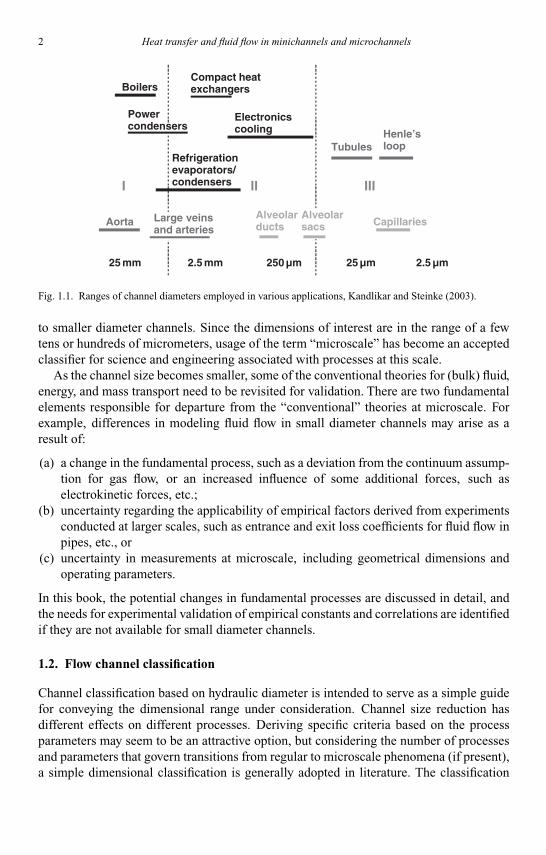
Figure 1.1 shows the ranges of channel dimensions employed in various systems.Interestingly, the biological systems with mass transport processes employ much smallerdimensions, whereas larger channels are used for fluid transportation. From an engineeringstandpoint, there has been a steady shift from larger diameters, on the order of 10–20 mm,
E-mail: [email protected]; [email protected]
1
Kandlikar I044527-Ch01.tex 29/10/2005 9: 20 Page 2
2 Heat transfer and fluid flow in minichannels and microchannels
25 mm 2.5 mm 250 µm 25 µm 2.5 µm
Boilers
Powercondensers
Compact heatexchangers
Refrigerationevaporators/condensers
Capillaries
Electronicscooling
Aorta
Henle’sloopTubules
I II III
Alveolarsacs
Alveolarducts
Large veinsand arteries
Fig. 1.1. Ranges of channel diameters employed in various applications, Kandlikar and Steinke (2003).
to smaller diameter channels. Since the dimensions of interest are in the range of a fewtens or hundreds of micrometers, usage of the term “microscale” has become an acceptedclassifier for science and engineering associated with processes at this scale.
As the channel size becomes smaller, some of the conventional theories for (bulk) fluid,energy, and mass transport need to be revisited for validation. There are two fundamentalelements responsible for departure from the “conventional” theories at microscale. Forexample, differences in modeling fluid flow in small diameter channels may arise as aresult of:
(a) a change in the fundamental process, such as a deviation from the continuum assump-tion for gas flow, or an increased influence of some additional forces, such aselectrokinetic forces, etc.;
(b) uncertainty regarding the applicability of empirical factors derived from experimentsconducted at larger scales, such as entrance and exit loss coefficients for fluid flow inpipes, etc., or
(c) uncertainty in measurements at microscale, including geometrical dimensions andoperating parameters.
In this book, the potential changes in fundamental processes are discussed in detail, andthe needs for experimental validation of empirical constants and correlations are identifiedif they are not available for small diameter channels.
1.2. Flow channel classification
Channel classification based on hydraulic diameter is intended to serve as a simple guidefor conveying the dimensional range under consideration. Channel size reduction hasdifferent effects on different processes. Deriving specific criteria based on the processparameters may seem to be an attractive option, but considering the number of processesand parameters that govern transitions from regular to microscale phenomena (if present),a simple dimensional classification is generally adopted in literature. The classification

Kandlikar I044527-Ch01.tex 29/10/2005 9: 20 Page 3
Chapter 1. Introduction 3
Table 1.1Channel dimensions for different types of flow for gases at one atmospheric pressure.
Channel dimensions (µm)
Continuum Transition Free molecularGas flow Slip flow flow flow
Air >67 0.67–67 0.0067–0.67 <0.0067Helium >194 1.94–194 0.0194–1.94 <0.0194Hydrogen >123 1.23–123 0.0123–1.23 <0.0123
Table 1.2Channel classification scheme.
Conventional channels >3 mm
Minichannels 3 mm ≥ D> 200 µmMicrochannels 200 µm ≥ D> 10 µmTransitional Microchannels 10 µm ≥ D> 1 µmTransitional Nanochannels 1 µm ≥ D> 0.1 µm
Nanochannels 0.1 µm ≥ D
D: smallest channel dimension
proposed by Mehendale et al. (2000) divided the range from 1 to 100 µm as microchannels,100 µm to 1 mm as meso-channels, 1 to 6 mm as compact passages, and greater than 6 mmas conventional passages.
Kandlikar and Grande (2003) considered the rarefaction effect of common gases atatmospheric pressure. Table 1.1 shows the ranges of channel dimensions that would fallunder different flow types.
In biological systems, the flow in capillaries occurs at very low Reynolds numbers. Adifferent modeling approach is needed in such cases. Also, the influence of electrokineticforces begins to play an important role. Two-phase flow in channels below 10 µm remainsunexplored. The earlier channel classification scheme of Kandlikar and Grande (2003) isslightly modified, and a more general scheme based on the smallest channel dimension ispresented in Table 1.2.
In Table 1.2, D is the channel diameter. In the case of non-circular channels, it is recom-mended that the minimum channel dimension; for example, the short side of a rectangularcross-section should be used in place of the diameter D. We will use the above classifi-cation scheme for defining minichannels and microchannels. This classification schemeis essentially employed for ease in terminology; the applicability of continuum theory orslip flow conditions for gas flow needs to be checked for the actual operating conditionsin any channel.
1.3. Basic heat transfer and pressure drop considerations
The effect of hydraulic diameter on heat transfer and pressure drop is illustrated in Figs. 1.2and 1.3 for water and air flowing in a square channel under constant heat flux and fully

Kandlikar I044527-Ch01.tex 29/10/2005 9: 20 Page 4
4 Heat transfer and fluid flow in minichannels and microchannels
10
100
1000
10,000
100,000
1,000,000
10 100 1000 10,000Hydraulic diameter (�side) of a square channel (µm)
Hea
t tr
ansf
er c
oeffi
cien
t (W
/m2
-k)
Air
Water
Fig. 1.2. Variation of the heat transfer coefficient with channel size for fully developed laminar flow of airand water.
developed laminar flow conditions. The heat transfer coefficient h is unaffected by the flowReynolds number (Re) in the fully developed laminar region. It is given by:
h = Nuk
Dh(1.1)
where k is the thermal conductivity of the fluid and Dh is the hydraulic diameter of thechannel. The Nusselt number (Nu) for fully developed laminar flow in a square channelunder constant heat flux conditions is 3.61. Figure 1.2 shows the variation of h for flowof water and air with channel hydraulic diameter under these conditions. The dramaticenhancement in h with a reduction in channel size is clearly demonstrated.
On the other hand, the friction factor f varies inversely with Re, since the product f · Reremains constant during fully developed laminar flow. The frictional pressure drop per unitlength for the flow of an incompressible fluid is given by:
pf
L= 2 fG2
ρD(1.2)
where pf /L is the frictional pressure gradient, f is the Fanning friction factor, G is themass flux, and ρ is the fluid density. For fully developed laminar flow, we can write:
f · Re = C (1.3)
where Re is the Reynolds number, Re = GDh/µ, and C is a constant, C = 14.23 for a squarechannel.
Figure 1.3 shows the variation of pressure gradient with the channel size for a squarechannel with G = 200 kg/m2 s, and for air and water assuming incompressible flow condi-tions. These plots are for illustrative purposes only, as the above assumptions may not be

Kandlikar I044527-Ch01.tex 29/10/2005 9: 20 Page 5
Chapter 1. Introduction 5
1.00E�01
1.00E�02
1.00E�03
1.00E�04
1.00E�05
1.00E�06
1.00E�07
1.00E�08
10 100 1000 10,000Hydraulic diameter (�side) of a square channel (µm)
Pre
ssur
e gr
adie
nt (
Pa/
m)
Air
Water
Fig. 1.3. Variation of pressure gradient with channel size for fully developed laminar flow of air and water.
valid for the flow of air, especially in smaller diameter channels. It is seen from Fig. 1.3that the pressure gradient increases dramatically with a reduction in the channel size.
The balance between the heat transfer rate and pressure drop becomes an importantissue in designing the coolant flow passages for the high-flux heat removal encounteredin microprocessor chip cooling. These issues are addressed in detail in Chapter 3 undersingle-phase liquid cooling.
1.4. Special demands of microscale biological applications
The use of minichannels, microchannels, and microfluidics in general is becoming increas-ingly important to the biomedical community. However, the transport and manipulation ofliving cells and biological macromolecules place increasingly critical demands on main-taining system conditions within acceptable ranges. For instance, human cells require anenvironment of 37◦C and a pH = 7.4 to ensure their continued viability. If these parametervalues stray more than 10% then cell death will result. All protein molecules themselveshave preferred pH environments, and large variations from this can cause (sometimesirreversible) denaturation and loss of biological activity due to unfolding.
High temperatures can also cause irreversible protein denaturation. However, in a poly-merase chain reaction, or PCR, the rapid cycling (∼1 min/cycle) of temperature between94◦C and 54◦C for 30–40 cycles is necessary to induce repeated denaturation and anneal-ing of DNA chains. Here, the microchannel geometry can be exploited due to the easeof changing the temperature of small liquid volumes, and in fact thermally driven naturalconvection can be used to achieve such temperature cycles (Krishnan et al., 2002).
Additionally, the concentrations of solutes, such as dissolved gases, nutrients, andmetabolic products, must be maintained within specified tolerances to ensure cell pro-liferation in microchannel bioreactors. Finally, local shear stresses can be critical insuspensions of biological particles. For instance, many cell types such as blood platelets

Kandlikar I044527-Ch01.tex 29/10/2005 9: 20 Page 6
6 Heat transfer and fluid flow in minichannels and microchannels
become activated to a highly adhesive state upon exposure to elevated shear stresses above10 dynes/cm2. Endothelial cells, which line the cardiovascular system, require a certainlevel of laminar shear stress on their luminal surface (≥0.5 dynes/cm2) or else they will notalign themselves properly and can express surface receptor molecules which induce chronicinflammation. At much higher shear stresses such as 1500 dynes/cm2, as can be producedaround sharp corners for very high liquid flow rates, red blood cells are known to “lyse”or rupture. This is especially critical when designing artificial blood pumps or implantablereplacement valves. All of these concerns must be separately addressed when develop-ing new microscale flow applications for the transport and manipulation of biologicalmaterials.
1.5. Summary
Microchannels are found in many biological systems where extremely efficient heat andmass transfer processes occur, such as lungs and kidneys. The channel size classificationis based on observations of many different processes, but its use is mainly in arrivingat a common terminology. The heat and mass transfer rates in small diameter channelsare also associated with a high pressure drop penalty for fluid flow. The fundamentals ofmicrochannels and minichannels in various applications are presented in this book.
1.6. Practice problems
Problem 1.1 Calculate the heat and mass transfer coefficients for airflow in a humanlung at various branches. Assume fully developed laminar flow conditions. Comment onthe differences between this idealized case and the realistic flow conditions.
Hint: Consult a basic anatomy book for the dimensions of the airflow passages and flowrates, and a heat and mass transfer book for laminar fully developed Nusselt numberand Sherwood number in a circular tube.
Problem 1.2 Calculate the Knudsen number for flow of helium flowing at a pressure of1 millitorr (1 torr = 1 mmHg) in 0.1-, 1-, 10-, and 100-mm diameter tubes. What type offlow model is applicable for each case?
Hint: Knudsen number is given by Kn = λ/Dh, and the mean free path λ is given byλ= (µ
√π/ρ
√2RT ), whereµ is the fluid viscosity, ρ is the fluid density, T is the absolute
temperature, and R is the gas constant.
Problem 1.3 Calculate the pressure drop for flow of water in a 15-mm long 100-µmcircular microchannel flowing at a temperature of 300 K and with a flow Reynolds numberof (a) 10, (b) 100, and (c) 1000. Also calculate the corresponding water flow rates in kg/sand ml/min.

Kandlikar I044527-Ch01.tex 29/10/2005 9: 20 Page 7
Chapter 1. Introduction 7
References
Kandlikar, S. G. and Grande, W. J., 2003, Evolution of microchannel flow passages – thermohydraulicperformance and fabrication technology, Heat Transfer Eng., 24(1), 3–17, 2003.
Kandlikar, S. G. and Steinke, M. E., 2003, Examples of microchannel mass transfer pro-cesses in biological systems, Proceedings of 1st International Conference on Minichannels andMicrochannels, Rochester, NY, April 24–25, Paper ICMM2003-1124. ASME, pp. 933–943.
Krishnan, M., Ugaz, V. M., and Burns, M. A., PCR in a Rayleigh–Benard convection cell, Science,298, 793.
Mehendale, S. S., Jacobi, A. M., and Shah, R. K., Fluid flow and heat transfer at micro- andmeso-scales with applications to heat exchanger design, Appl. Mech. Rev., 53, 175–193.

This page intentionally left blank
Kandlikar I044527-Ch02.tex 26/10/2005 18: 8 Page 9
Chapter 2
SINGLE-PHASE GAS FLOW IN MICROCHANNELS
Stéphane Colin
Department of Mechanical Engineering, National Institute of Applied Sciences of Toulouse,31077 Toulouse, France
Microfluidics is a rather young research field, born in the early eighties. Its older relativefluidics was in fashion in the sixties to seventies. Fluidics seems to have started in USSR in1958, then developed in USA and Europe first for military purposes with civil applicationsappearing later. At that time, fluidics was mainly concerned with inner gas flows in devicesinvolving millimetric or sub-millimetric sizes. These devices were designed to performthe same actions (amplification, logic operations, diode effects, etc.) as their electriccounterparts. The idea was to design pneumatically, in place of electrically, suppliedcomputers. The main applications were the concern of the spatial domain, for whichelectric power overload was indeed an issue due to the electric components of the time thatgenerated excessive magnetic fields and dissipated too much thermal energy to be safein a confined space. Most of the fluidic devices were etched in a substrate, by means ofconventional machining techniques, or by insolation techniques applied on specific resinswhere masks protected the parts to preserve. The rapid development of microelectronicsput a sudden end to pneumatic computers, but these two decades were particularly usefulto enhance our knowledge about gas flows in minichannels or mini pneumatic devices.
As microfluidics concerns smaller sizes – the inner sizes of Micro-Electro-Mechanical-Systems (MEMS) – new issues have to be considered in order to accurately model gasmicroflows. These issues are mainly due to rarefaction effects, which typically must betaken into account when characteristic lengths are of the order of 1 µm, under usualtemperature and pressure conditions.
In this chapter, the role of rarefaction is explained and its consequences on the behav-ior of gas flows in microchannels are detailed. The main theoretical and experimentalresults from the literature about pressure-driven, steady or pulsed gas microflows are sum-marized. Heat transfer in microchannels and thermally driven gas microflows are alsodescribed. They are particularly interesting for vacuum generation, using microsystemswithout moving parts.
E-mail: [email protected]
9
Kandlikar I044527-Ch02.tex 26/10/2005 18: 8 Page 10
10 Heat transfer and fluid flow in minichannels and microchannels
2.1. Rarefaction and wall effects in microflows
In microfluidics, theoretical knowledge for gas flows is currently more advanced thanthat for liquid flows (Colin, 2004). Concerning the gases, the issues are actually moreclearly identified: the main micro-effect that results from shrinking down the devices sizeis rarefaction. This allows us to exploit the strong, although not complete analogy betweenmicroflows and low pressure flows that has been extensively studied for more than 50 yearsand particularly for aerospace applications.
2.1.1. Gas at the molecular level
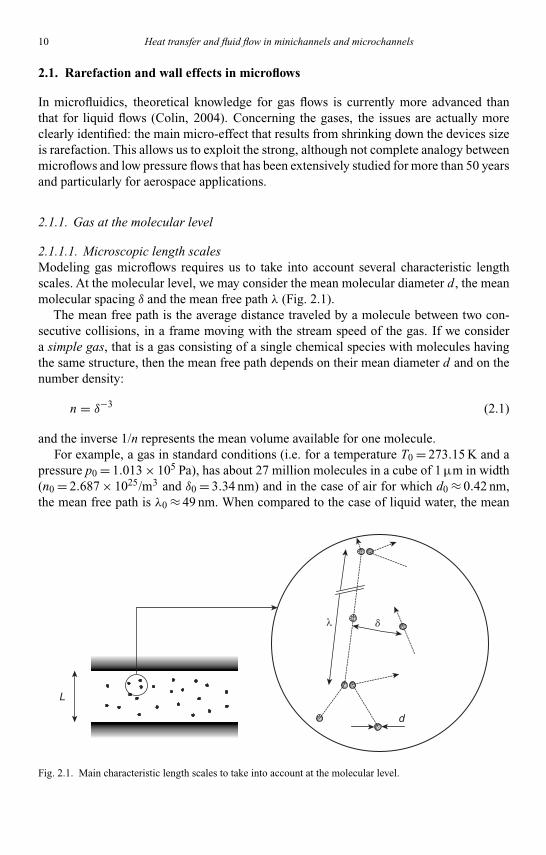
2.1.1.1. Microscopic length scalesModeling gas microflows requires us to take into account several characteristic lengthscales. At the molecular level, we may consider the mean molecular diameter d, the meanmolecular spacing δ and the mean free path λ (Fig. 2.1).
The mean free path is the average distance traveled by a molecule between two con-secutive collisions, in a frame moving with the stream speed of the gas. If we considera simple gas, that is a gas consisting of a single chemical species with molecules havingthe same structure, then the mean free path depends on their mean diameter d and on thenumber density:
n = δ−3 (2.1)
and the inverse 1/n represents the mean volume available for one molecule.For example, a gas in standard conditions (i.e. for a temperature T0 = 273.15 K and a
pressure p0 = 1.013 × 10⁵ Pa), has about 27 million molecules in a cube of 1 µm in width(n0 = 2.687 × 1025/m3 and δ0 = 3.34 nm) and in the case of air for which d0 ≈ 0.42 nm,the mean free path is λ0 ≈ 49 nm. When compared to the case of liquid water, the mean
L
dλ
d
Fig. 2.1. Main characteristic length scales to take into account at the molecular level.

Kandlikar I044527-Ch02.tex 26/10/2005 18: 8 Page 11
Chapter 2. Single-phase gas flow in microchannels 11
molecular diameter of each are nearly equal, but the mean molecular spacing is about10 times smaller and the mean free path is 105 times smaller than air!
2.1.1.2. Binary intermolecular collisions in dilute simple gasesGases that satisfy
d
δ 1 (2.2)
are said to be dilute gases. In that case, most of the intermolecular interactions are binarycollisions. Conversely, if Eq. (2.2) is not verified, the gas is said to be a dense gas. Thedilute gas approximation, along with the equipartition of energy principle, leads to theclassic kinetic theory and the Boltzmann transport equation.
With this approximation, the mean free path of the molecules may be expressed as theratio of the mean thermal velocity c′ to the collision rate ν:
λ = c′ν
=√
8RT /π
ν(2.3)
The thermal velocity c′ of a molecule is the difference between its total velocity c andthe local macroscopic velocity u of the flow (cf. Section 2.1.2), and its mean valuec′ = √
8RT /π, which depends on the temperature T and on the specific gas constant R,is calculated from the Boltzmann equation. The estimation of the collision rate and con-sequently of the mean free path depends on the model chosen for describing the elasticbinary collision between two molecules. Such a model also allows estimation of the totalcollision cross-section
σt = πd2 (2.4)
in the collision plane and the mean molecular diameter d (Fig. 2.2), as well as the dynamicviscosity µ as a function of the temperature.
A collision model generally requires the definition of the force F exerted between thetwo considered molecules. This force is actually repulsive at short distances and weaklyattractive at large distances. Different approximated models are proposed to describe thisforce. The more classic one is the so-called inverse power law (IPL) model or point center
d
st � pd2
Fig. 2.2. Total collision cross-section in the collision plane.

Kandlikar I044527-Ch02.tex 26/10/2005 18: 8 Page 12
12 Heat transfer and fluid flow in minichannels and microchannels
of repulsion model (Bird, 1998). It only takes into account the repulsive part of the forceand assumes that
F = |F| = κ
rη(2.5)
This derives from an intermolecular potential
φ = κ
(η− 1)rη−1 (2.6)
where κ, as well as the exponent η have a constant value and r denotes the distance betweenthe two molecules centers. Using the Chapman–Enskog theory, this model leads to a lawof viscosity in the form
µ = µ0
(T
T0
)ω(2.7)
with
ω = η+ 3
2(η− 1)(2.8)
The collision rate may be deduced as (Lengrand and Elizarova, 2004)
ν = 4(
5
2− ω
)ω− 12
�
(5
2− ω
)nσt0
(T
T0
) 12 −ω√RT
π(2.9)
where �( j) = ∫∞0 x j−1 exp (−x)dx is the Euler, or gamma function and T0 is a reference
temperature for which the total collision cross-section σt0 is calculated. From Eq. (2.3),we can see that the mean free path
λ = 1√
2( 5
2 − ω)ω− 1
2 �( 5
2 − ω)nσt0
(T
T0
)ω− 12
(2.10)
is proportional to Tω− 12 and inversely proportional to the number density n.
The simplest collision model is the hard sphere (HS) model, which assumes that thetotal collision cross-section σt is constant and for which the viscosity is proportional tothe square root of the temperature. Actually, the HS model may be described from the IPLwith the exponent η→ ∞ and ω= 1/2.
Bird, who proposed the variable hard sphere (VHS) model for applications to the MonteCarlo method (DSMC, cf. Section 2.2.4.2), has improved the HS model. The VHS modelmay be considered as a HS model with a diameter d that is a function of the relative velocitybetween the two colliding molecules. The Chapman–Enskog method leads to a viscosity
µVHS = 15 m√πRT
8( 5
2 − ω)ω− 1
2 �( 9
2 − ω)σt0
(T
T0
)ω− 12
(2.11)
Kandlikar I044527-Ch02.tex 26/10/2005 18: 8 Page 13
Chapter 2. Single-phase gas flow in microchannels 13
which verifies Eq. (2.7) and where m is the molecular mass. By eliminating σt0 betweenEqs. (2.9) or (2.10) and (2.11) and noting that �( j + 1) = j�( j), the mean free path andthe collision rate for a VHS model may be expressed as functions of the viscosity and thetemperature:
νVHS = ρRT
µ
30(7 − 2ω)(5 − 2ω)
(2.12)
and
λVHS = µ
ρ√
2πRT
2(7 − 2ω)(5 − 2ω)
15(2.13)
with ρ= mn as the local density.Another classic model is the Maxwell molecules (MM) model. It is a special case of the
IPL model withη= 5 andω= 1. Actually, the HS and the MM models may be considered asthe limits of the more realistic VHS model, since real molecules generally have a behaviorwhich corresponds to an intermediate value 1/2 ≤ω≤ 1. Another expression is frequentlyencountered in the literature: for example, Karniadakis and Beskok (2002) or Nguyenand Wereley (2002) use the formula λM = √
π/2µ/(ρ√
RT ) proposed by Maxwell in 1879(Eq. (2.57)).
Other binary collision models based on the IPL assumption are described in the litera-ture. Koura and Matsumoto (1991; 1992) introduced the variable soft sphere (VSS) model,which differs from the VHS model by a different expression of the deflection angle takenby the molecule after a collision. The VSS model leads to a correction of the mean freepath and the collision rate values:
λVSS = βλVHS νVSS = νVHS
β(2.14)
where β= 6α/[(α+ 1)(α+ 2)] and the value of α is generally between 1 and 2 (Bird, 1998).Thus, the correction introduced by the VSS model in the mean free path and in the collisionrate remains limited, less than 3%. For α= 1, the VSS model reduces to the VHS model.
Finally, some models can take into account the long-range attractive part of the forcebetween two molecules by adding a uniform attractive potential (square-well model), oran IPL attractive component (Sutherland, Hassé and Cook or Lennard–Jones potentialmodels) to the HS model. For example, the Lennard–Jones potential is
φ = κ
(η− 1)rη−1 − κ′
(η′ − 1)rη′−1(2.15)
and the widely used Lennard–Jones 12-6 model corresponds to η= 13 and η′ = 7. Thegeneralized hard sphere (GHS) model (Hassan and Hash, 1993) is a generalized modelthat combines the computational simplicity of the VHS model and the accuracy of compli-cated attractive–repulsive interaction potentials. More recently, the variable sphere (VS)molecular model proposed by Matsumoto (2002) provides consistency for diffusion andviscosity coefficients with those of any realistic intermolecular potential.

Kandlikar I044527-Ch02.tex 26/10/2005 18: 8 Page 14
14 Heat transfer and fluid flow in minichannels and microchannels
Table 2.1Mean free path, dynamic viscosity, and collision rate for classic IPL collision models.
F = κ
rηµ∝ Tω ν= k1
ρRT
µλ= k2
µ
ρ√
RTModel η ω k1 k2
HS ∞ 1
2
5
4
16
5√
2π≈ 1.277
VHS η ω= η+ 3
2(η− 1)
30
(7 − 2ω)(5 − 2ω)
2(7 − 2ω)(5 − 2ω)
15√
2π
MM 5 1 2
√2
π≈ 0.798
VSS η ω= η+ 3
2(η− 1)
5(α+ 1)(α+ 2)
α(7 − 2ω)(5 − 2ω)
4α(7 − 2ω)(5 − 2ω)
5(α+ 1)(α+ 2)√
2π
Table 2.1 resumes the relationships between the collision rate, the mean free path, theviscosity, the density and the temperature for classic IPL collision models. As the meanfree path λ is an important parameter for the simulation of gas microflows (cf. Section2.1.2), we should be careful when comparing some theoretical results from the literatureand verify from which model λ has been calculated. Note that for the formula of Maxwell,k2,M = √
π/2 is 2% lower than the value k2,HS = 16/(5√
2π) obtained from a HS model.Equation (2.11) is also interesting because it allows estimation of the mean molecular
diameter d from viscosity data and a VHS model. Table 2.2 gives the value of d fordifferent gases under standard conditions, obtained by Bird (1998), from a VHS or a VSShypothesis. The ratio δ0/d is calculated for the mean value d of dVHS and dVSS. For anygas, we can see that the condition (2.2) is roughly verified and the different gases canreasonably be considered as dilute gases under standard conditions. However, the dilutegas approximation will be better for He than for SO2.
2.1.2. Continuum assumption and thermodynamic equilibrium
When applicable, the continuum assumption is very convenient since it erases the moleculardiscontinuities, by averaging the microscopic quantities on a small sampling volume. Allmacroscopic quantities of interest in classic fluid mechanics (densityρ, velocity u, pressurep, temperature T , etc.) are assumed to vary continuously from point to point within the flow.
For example, if we consider an air flow in a duct, for which the macroscopic velocityvaries from 0 to 1 m/s and is parallel to the axis of the duct, the velocity of a molecule isof the order of 1 km/s and may take any direction. Similar considerations also concern theother mechanical and thermodynamic quantities.
In order to respect the continuum assumption, the microscopic fluctuations shouldnot generate significant fluctuations of the averaged quantities. Consequently, the size of arepresentative sampling volume must be large enough to erase the microscopic fluctuations,but it must also be small enough to point out the macroscopic variations, such as velocity or

Kandlikar I044527-Ch02.tex 26/10/2005 18: 8 Page 15
Chapter 2. Single-phase gas flow in microchannels 15
Table 2.2Molecular weight, dynamic viscosity and mean molecular diameters under standard conditions (p0 = 1.013 ×10⁵ Pa and T0 = 273.15 K) estimated from a VHS or a VSS model (data from Bird (1998)) with correspondingvalues of the ratio δ0/d.
M × 103 µ0 × 107
Gas (kg/mol) (N-s/m2) ω dVHS (pm) α dVSS (pm) δ0/d
Sea level air 28.97 171.9 0.77 419 – – 7.97Ar 39.948 211.7 0.81 417 1.40 411 8.06CH4 16.043 102.4 0.84 483 1.60 478 6.95Cl2 70.905 123.3 1.01 698 – – 4.78CO 28.010 163.5 0.73 419 1.49 412 8.04CO2 44.010 138.0 0.93 562 1.61 554 5.98H2 2.0159 84.5 0.67 292 1.35 288 11.51HCl 36.461 132.8 1.00 576 1.59 559 5.88He 4.0026 186.5 0.66 233 1.26 230 14.42Kr 83.80 232.8 0.80 476 1.32 470 7.06N2 28.013 165.6 0.74 417 1.36 411 8.06N2O 44.013 135.1 0.94 571 – – 5.85Ne 20.180 297.5 0.66 277 1.31 272 12.16NH3 17.031 92.3 1.10 594 – – 5.62NO 30.006 177.4 0.79 420 – – 7.95O2 31.999 191.9 0.77 407 1.40 401 8.26SO2 64.065 116.4 1.05 716 – – 4.66Xe 131.29 210.7 0.85 574 1.44 565 5.86
Microscopic fluctuations
Macroscopic variations
Macroscopicquantity
Samplingvolume
Representativesampling volume
Controlvolume
Fig. 2.3. The existence of a representative sampling volume (shaded area) is necessary for the continuumassumption to be valid.
pressure gradients of interest in the control volume (Fig. 2.3). If the shaded area on Fig. 2.3does not exist, the sampling volume is not representative and the continuum assumptionis not valid.
It may be considered that sampling a volume containing 10,000 molecules leads to1% statistical fluctuations in the macroscopic quantities (Karniadakis and Beskok, 2002).Such a fluctuation level needs a sampling volume which characteristic length lSV verifies
Kandlikar I044527-Ch02.tex 26/10/2005 18: 8 Page 16
16 Heat transfer and fluid flow in minichannels and microchannels
lSV/δ= 104/3 ≈ 22. Consequently, the control volume must have a much higher character-istic length L, that is
L
δ� 104/3 (2.16)
so that the statistical fluctuations can be neglected. For example, for air at standard con-ditions, the value of lSV corresponding to 1% statistical fluctuations is 72 nm. This iscomparable to the value of the mean free path λ0 = 49 nm.
Moreover, the continuum approach requires that the sampling volume is in thermo-dynamic equilibrium. For the thermodynamic equilibrium to be respected, the frequency ofthe intermolecular collisions inside the sampling volume must be high enough. This impliesthat the mean free path λ= c′/ν must be small compared with the characteristic length lSVof the sampling volume, itself being small compared with the characteristic length L ofthe control volume. As a consequence, the thermodynamic equilibrium requires that
λ
L 1 (2.17)
This ratio
Kn = λ
L(2.18)
is called the Knudsen number and it plays a very important role in gaseous microflows(see Section 2.1.3). If λ is obtained from an IPL collision model,
λ = k2µ/ρ√
RT (2.19)
with k2 given by Table 2.1, and the Knudsen number can be related to the Reynolds number
Re = ρuL
µ(2.20)
and the Mach number
Ma = u
a(2.21)
by the relationship
Kn = k2√γ
Ma
Re(2.22)
Here, γ is the ratio of the specific heats of the gas and a, the local speed of sound, witha = √
γRT for an ideal gas (Anderson, 1990), which is verified for a dilute gas (cf. Sec-tion 2.2.1). Equation (2.22) shows the link between rarefaction (characterized by Kn) andcompressibility (characterized by Ma) effects, the latter having to be taken into accountif Ma> 0.3.

Kandlikar I044527-Ch02.tex 26/10/2005 18: 8 Page 17
Chapter 2. Single-phase gas flow in microchannels 17
The limits that correspond to Eqs. (2.2), (2.16) and (2.17), with the indicative values(δ/d = 7, L/δ= 100 and λ/L = 0.1) proposed by Bird (Bird, 1998), are shown in Fig. 2.4. Inthis figure, the mean free path has been estimated with an HS model, for which Eq. (2.10)can be written using Eq. (2.4) and ω= 1/2, in the form
λHS = δ3
√2πd2
(2.23)
Thus λ/L = (δ/d)3(d/L)(1/√
2π) and the thermodynamic equilibrium limit λ/L = 0.1 isa straight line with a slope equal to –3 in the log–log plot of Fig. 2.4.
2.1.3. Rarefaction and Knudsen analogy
It is now clear that the similitude between low pressure and confined flows is not complete,since the Knudsen number is not the only parameter to take into account (cf. Fig. 2.4.).
107
106
105
104
103
102
101
100
100101102
Dense gasDilute gas
Thermodynamicdisequilibrium
Significantstatistical
fluctuations
Negligiblestatistical
fluctuations
Thermodynamicequilibrium
L/d � 100
d/d
� 7
d/d
L/d
l/L � 0.1
Fig. 2.4. Limits of the main approximations for the modeling of gas microflows (from Bird (1998)).

Kandlikar I044527-Ch02.tex 26/10/2005 18: 8 Page 18
18 Heat transfer and fluid flow in minichannels and microchannels
However, it is convenient to differentiate the flow regimes in function of Kn, and thefollowing classification, although tinged with empiricism, is usually accepted:
● For Kn< 10−3, the flow is a continuum flow (C) and it is accurately modeled by thecompressible Navier–Stokes equations with classical no-slip boundary conditions.
● For 10−3 <Kn< 10−1, the flow is a slip flow (S) and the Navier–Stokes equations remainapplicable, provided a velocity slip and a temperature jump are taken into account atthe walls. These new boundary conditions point out that rarefaction effects becomesensitive at the wall first.
● For 10−1 <Kn< 10, the flow is a transition flow (T) and the continuum approach ofthe Navier–Stokes equations is no longer valid. However, the intermolecular collisionsare not yet negligible and should be taken into account.
● For Kn> 10, the flow is a free molecular flow (M) and the occurrence of intermolecularcollisions is negligible compared with the one of collisions between the gas moleculesand the walls.
These different regimes will be detailed in the following sections. Their limits areonly indicative and could vary from one case to another, partly because the choice of thecharacteristic length L is rarely unique. For flows in channels, L is generally the hydraulicdiameter or the depth of the channel. In complex geometrical configurations, it is generallypreferable to define L from local gradients (e.g. of the density ρ: L = 1/|∇ρ/ρ|) ratherthan from simple geometrical considerations (Gad-el-Hak, 1999); the Knudsen numberbased on this characteristic length is the so-called local rarefaction number (Lengrand andElizarova, 2004). Figure 2.5 locates these different regimes for air in standard conditions.For comparison, the cases or helium and sulphur dioxide are also represented. For SO2,the dilute gas assumption is less valid than for air and He, and the binary intermolecularcollision models described in Section 2.1.1.2 could be inaccurate. The shaded area roughlyrepresents the domain of validity for classic gas flow models (C).
The relationship with the characteristic length L expressed in micrometers is illustratedin Fig. 2.6, which shows the typical ranges covered by fluidic microsystems describedin the literature. Typically, most of the microsystems which use gases work in the slipflow regime, or in the early transition regime. In simple configurations, such flows canbe analytically or semi-analytically modeled. The core of the transition regime relatesto more specific flows that involve lengths under 100 nanometers, as it is the case for aCouette flow between a hard disk and a read–write head. In that regime, the only theoreticalmodels are molecular models that require numerical simulations. Finally, under the effectof both low pressures and small dimensions, more rarefied regimes can occur, notablyinside microsystems dedicated to vacuum generation.
2.1.4. Wall effects
We have seen that initial deviations from the classic continuum models appear when weshrink down the characteristic length L of the flow with respect to the boundary conditions.It is logical that the first sources of thermodynamic disequilibria appear on the boundarybecause at the wall there are fewer interactions between the gas molecules than in the coreof the flow.

Kandlikar I044527-Ch02.tex 26/10/2005 18: 8 Page 19
Chapter 2. Single-phase gas flow in microchannels 19
Standard conditions for He air SO2
(C)
(S)
(T)
(M)
107
106
105
104
103
102
101
100
100101102d/d
Kn � 10 �
3
Kn � 10 �
1
Kn � 10 �
1
d/d
� 7
L/d
Fig. 2.5. Gas flow regimes as a function of the Knudsen number.
Kn
L (µm)
102
101
100
10�1
10�2
10�3
10�4
10�2 10�1 100 101 102
Free molecular flow (M)
Transitional flow (T)
Slip flow (S)
Continuum flow (C)
Microvalves
Micronozzles
Microflowsensors
Microchannelsmicropumps
Hard disk drives
Fig. 2.6. Gas flow regimes for usual microsystems (from Karniadakis and Beskok (2002)).

Kandlikar I044527-Ch02.tex 26/10/2005 18: 8 Page 20
20 Heat transfer and fluid flow in minichannels and microchannels
Actually, the walls play a crucial role in gas microflows. First, shrinking system sizesresults in an increase of surface over volume effects. It is interesting for heat transferenhancement, but it also requires an excellent knowledge of the velocity, as well as thetemperature and boundary conditions. The velocity slip and the temperature jump observedat the wall in the slip flow regime strongly depend on the nature and on the state of thewall, in relation to the nature of the gas. Thus, the roughness of the wall and the chemicalaffinity between the wall and the gas, although often not properly known, could highlyaffect the fluid flow and the heat transfer.
2.2. Gas flow regimes in microchannels
Usually, the regime of gas flow in a macrochannel refers to viscous and compressibilityeffects, respectively quantified by the Reynolds number Re and the Mach number Ma.For low Reynolds numbers (typically for Re< 2000), the flow is laminar and it becomesturbulent for higher values of Re. For Ma< 1, the flow is subsonic and for Ma> 1, it issupersonic. Typically, if Ma> 0.3, compressibility effects should be taken into account.
In microchannels on the other hand, the main effects are rarefaction effects, essen-tially quantified by the Knudsen number Kn. Consequently, the regime usually refers tothese effects, according to the classification given in Section 2.1.3, and flows are con-sidered as microflows for Kn> 10−3. Actually, Eq. (2.22) shows that for a dilute gas,Re = k2
√γ Ma/Kn, where k2
√γ is of the order of unity, which implies that for subsonic
microflows, viscous effects are predominant and the flows are laminar.The models used to describe gas flows in microchannels depend on the rarefaction
regime. The main models are presented in Fig. 2.7, with the rough values of Kn for which
Eul
er e
quat
ions
Kn
1010�3 10�10
Navier–Stokes equationswith no-slip BC
Navier–Stokes equationswith first-order slip BC
QGD or QHD equationswith first-order slip BC
orNavier–Stokes equationswith second-order slip BC
Burnett equationswith slip BC
DSMC or lattice Boltzmann
Fig. 2.7. Gas flow regimes and main models according to the Knudsen number. BC: boundary condition.

Kandlikar I044527-Ch02.tex 26/10/2005 18: 8 Page 21
Chapter 2. Single-phase gas flow in microchannels 21
each of them is applicable, that is valid and really interesting to use. The limits are indicativeand may vary according to the considered configurations.
These models are described in the following sections. Among the three main rarefiedregimes (slip flow, transition flow and molecular flow), the slip flow regime is more speciallydetailed, since it is the most frequently encountered (cf. Fig. 2.6) and it allows analytic orsemi-analytic developments. Moreover, the gas is considered as a dilute gas, which makesvalid the ideal gas assumption.
2.2.1. Ideal gas model
The classic equation of state for an ideal gas,
p = ρRT = nkBT (2.24)
is also called the Boyle–Mariotte’s law. Here, p is the pressure and ρ= mn isthe density, kB = R/N = (M/N )(R/M ) = mR = 1.38065 J/K is the Boltzmann constant,R = 8.314511 J/mol/K being the universal gas constant, N = 6.022137 × 10²³ mol−1, theAvogadro’s number and M, the molecular weight. Equation (2.24) may be obtained from amolecular analysis, assuming that the gas is a dilute gas in thermodynamic equilibrium.
If the thermodynamic equilibrium is not verified, Eq. (2.24) remains valid, providingthe thermodynamic temperature T is replaced with the translational kinetic temperatureTtr , which measures the mean translational kinetic energy of the molecules. The specificideal gas constant
R = cp − cv (2.25)
is the difference between the specific heats
cp = ∂h
∂T
∣∣∣∣p
(2.26)
and
cv = ∂e
∂T
∣∣∣∣v
(2.27)
where e is the internal specific energy, v = 1/ρ is the specific volume and h is the specificenthalpy. For an ideal gas, the specific heats are constant and their ratio is the index
γ = cp
cv(2.28)
Therefore, for an ideal gas,
cv = 1
γ − 1R cp = γ
γ − 1R (2.29)

Kandlikar I044527-Ch02.tex 26/10/2005 18: 8 Page 22
22 Heat transfer and fluid flow in minichannels and microchannels
The specific heat ratio is constant for a monatomic gas (γ = 5/3) but it is dependent of thetemperature for a diatomic gas, with a value close to 7/5 near atmospheric conditions.
Finally, we can note that for an ideal gas and an IPL collision model, the Knudsennumber can be written as:
Kn = k2µ(T )
ρ√
RT L= k2µ(T )
√RT
pL(2.30)
with the value of k2 given in Table 2.1.
2.2.2. Continuum flow regime
The classic continuum flow regime (which corresponds to the shaded area in Fig. 2.5) maybe accurately modeled by the compressible Navier–Stokes equations, the ideal gas equationof state, and classic boundary conditions that express the continuity of temperature andvelocity between the fluid and the wall.
2.2.2.1. Compressible Navier–Stokes equationsThe compressible Navier–Stokes equations are the governing conservation laws for mass,momentum and energy. These laws are written assuming that the fluid is Newtonian, sothat the stress tensor
σ′ = −p I + σ (2.31)
is a linear function of the velocity gradients. Thus, the viscous stress tensor has the formσ =µ[∇ ⊗ u + (∇ ⊗ u)T ] + ζ(∇ · u)I, where u is the velocity vector, I is the unit tensor,µ is the dynamic viscosity and ζ is the second coefficient of viscosity, or Lamé coefficient.With Stokes’ hypothesis, 2µ+ 3ζ= 0, which expresses that the changes of volume do notinvolve viscosity, the viscous stress tensor may be written as σ =µ[∇ ⊗ u + (∇ ⊗ u)T −(2/3)(∇ · u)I]. The validity of this assumption is discussed in Gad-el-Hak (1995).
The Navier–Stokes equations also assume that the fluid follows the Fourier law ofdiffusion. Thus, the heat flux vector q is related to the temperature gradient by q = −k∇T ,where the thermal conductivity k is a function of the temperature.
With the above relations, the compressible Navier–Stokes equations may be written as:
∂ρ
∂t+ ∇ · (ρu) = 0 (2.32)
∂(ρu)
∂t+ ∇ ·
(ρu ⊗ u − µ
[∇ ⊗ u + (∇ ⊗ u)T − 2
3(∇ · u)I
])+ ∇p = f (2.33)
∂E
∂t+ ∇ ·
((E + p)u − µ
[∇ ⊗ u + (∇ ⊗ u)T − 2
3(∇ · u)I
]· u − k∇T
)= f · u (2.34)

Kandlikar I044527-Ch02.tex 26/10/2005 18: 8 Page 23
Chapter 2. Single-phase gas flow in microchannels 23
These conservation equations are respectively the continuity (2.32), the momentum(2.33) and the energy (2.34) equations. The total energy per unit volume
E = ρ
(1
2u · u + e
)(2.35)
is a function of the internal specific energy e that may be written for an ideal gas, usingEqs. (2.24)–(2.26) and (2.28):
e = p
ρ(γ − 1)(2.36)
The external volume forces f (gravitational forces, magnetic forces, etc.) are generallynegligible in gas flow. It is even more the case in gas microflows, since the volume oversurface ratio decreases with the characteristic length L and consequently, in microscalegeometries, volume effects may be neglected when compared to surface effects.
2.2.2.2. Classic boundary conditionsThe previous set of Eqs. (2.24) and (2.32)–(2.34) must be completed with appropriateboundary conditions. In the continuum flow regime, they express the continuity of thevelocity,
u|w = uwall (2.37)
and of the temperature,
T |w = Twall (2.38)
at the wall, the subscripts “wall” relating to the wall itself, and “w” to the conditions inthe fluid at the wall.
2.2.3. Slip flow regime
Actually, whatever the Knudsen number (even for very low values of Kn), there is in theneighborhood of the wall a domain in which the gas is out of equilibrium. This domain iscalled the Knudsen layer and has a thickness in the order of the mean free path. For verylow Knudsen numbers (in the continuum flow regime), the effect of the Knudsen layeris negligible. In the slip flow regime, which is roughly in the range 10−3 < Kn< 10−1,the Knudsen layer must be taken into account. Actually, the flow in the Knudsen layercannot be analyzed from continuum by use of the Navier–Stokes equations, for example.But for Kn< 10−1, its thickness is small enough and the Knudsen layer can be neglected,providing the boundary conditions (2.37)–(2.38) are modified and express a velocity slip,as well as a temperature jump at the wall (Section 2.2.3.2).
Thus, the Navier–Stokes equations remain applicable, but it could also be convenientto replace them by another set of conservation equations, such as the quasi-hydrodynamic(QHD) equations or the quasi-gasdynamic (QGD) equations (see Section 2.2.3.1).

Kandlikar I044527-Ch02.tex 26/10/2005 18: 8 Page 24
24 Heat transfer and fluid flow in minichannels and microchannels
2.2.3.1. Continuum NS–QGD–QHD equationsIn a generic form, the conservation equations may be written in the following way:
∂ρ
∂t+ ∇ · JEQ = 0 (2.39)
for the continuity equation,
∂(ρu)
∂t+ ∇ · (JEQ ⊗ u − σEQ) + ∇p = 0 (2.40)
for the momentum equation and
∂E
∂t+ ∇ ·
(E + p
ρJEQ − σEQ · u + qEQ
)= 0 (2.41)
for the energy equation. In these equations, JEQ is the mass flux vector, σEQ, the vis-cous stress tensor and qEQ, the heat flux vector. The external volume forces f have beenneglected.
In the case of the Navier–Stokes equations (EQ ≡ NS) these variables have the form:
JNS = ρu (2.42)
σNS = µ[∇⊗u+(∇⊗u)T ]+ζ(∇·u)I = µ
[∇ ⊗ u + (∇ ⊗ u)T − 2
3(∇ · u)I
](2.43)
qNS = −k ∇T (2.44)
These lead to the previous Eqs. (2.32)–(2.34). In the Navier–Stokes equations, the densityρ, the pressure p and the velocity u correspond to space averaged instantaneous quantities.
From spatiotemporal considerations, the QGD and the QHD equations may be obtained(Lengrand and Elizarova, 2004). They are based on the same governing conservation laws(2.39)–(2.41), but these laws are closed with a different definition of JEQ, σEQ and qEQ.Dissipative terms are added, which involve a parameter τ. This parameter
τ = γµ
Sc ρ a2 (2.45)
is a time characteristic of the temporal averaging. Here, Sc =µ/(ρD) is the Schmidt num-ber, which represents the ratio of the diffusive mass over the diffusive momentum fluxes.In the expression of Sc, D is the diffusion coefficient, which can be expressed as a functionof α and ω for a VSS molecule. Thus, for a VSS molecule,
Sc = 5(2 + α)
3(7 − 2ω)α(2.46)
which reduces to 5/6 for a HS model. For an ideal gas, a2 = γRT and τ may be written as:
τ = 1
Sc
µ
p(2.47)
Kandlikar I044527-Ch02.tex 26/10/2005 18: 8 Page 25
Chapter 2. Single-phase gas flow in microchannels 25
The QGD equations are appropriate for dilute gases. For these equations (EQ ≡ QGD):
JQGD = JNS − τ[∇ · (ρu ⊗ u) + ∇p] (2.48)
σQGD = σNS + τ[u ⊗ (ρu · (∇ ⊗ u) + ∇p) + I(u · ∇p + γp∇ · u)] (2.49)
qQGD = qNS − τρu[u · ∇e + pu · ∇(1/ρ)] (2.50)
From Eqs. (2.18), (2.19), (2.24) and (2.47), we can deduce that for a dilute gas and an IPLcollision model,
τ = Kn
Sc
1
k2
L√RT
(2.51)
Therefore, [τ∇](Kn→0) → 0, which shows that the above QGD equations degenerate intothe classic NS equations when rarefaction is negligible.
Another set of equations, the QHD equations, are appropriate to dense gases. In thatcase (EQ ≡ QHD):
JQHD = JNS − τ[ρu · (∇ ⊗ u) + ∇p] (2.52)
σQHD = σNS + τu ⊗ (ρu · (∇ ⊗ u) + ∇p) (2.53)
qQHD = qNS (2.54)
They also bring additional terms to the NS equations, which are proportional to theparameter τ.
2.2.3.2. First-order slip boundary conditionsFrom a series of experiments at low pressures performed in 1875, Kundt and Warburgwere probably the first who pointed out that for a flow of rarefied gas, slipping occurs atthe walls (Kennard, 1938). For a gas flowing in the direction s parallel to the wall, the slipvelocity may be written as:
uslip = us − uwall = ξ∂us
∂n
∣∣∣∣w
(2.55)
where ξ is a length commonly called the coefficient of slip and n is the normal direction,exiting the wall. With appropriate assumptions, it is possible to calculate the magnitude ofthe coefficient of slip from the kinetic theory of gases.
Following a paper initially dealing with stresses in rarefied gases due to temperaturegradients (Maxwell, 1879), Maxwell added an appendix on the advise of a referee, withthe aim of expressing the conditions which must be satisfied by a gas in contact with asolid body. Maxwell treated the surface as something intermediate between a perfectlyreflecting and a perfectly absorbing surface. Therefore, he assumed that for every unit

Kandlikar I044527-Ch02.tex 26/10/2005 18: 8 Page 26
26 Heat transfer and fluid flow in minichannels and microchannels
n
s
(a) (b)
Fig. 2.8. Maxwell hypothesis. (a) Perfect (specular) reflection of a fraction 1 − σ of the molecules.(b) Absorption and diffuse reemission of a fraction σ of the molecules.
of area, a fraction σ of the molecules is absorbed by the surface (due to the roughnessof the wall, or to a condensation–evaporation process (Kennard, 1938)) and is afterwardsreemitted with velocities corresponding to those in still gas at the temperature of thewall. The other fraction, 1 − σ, of the molecules is perfectly reflected by the wall (Fig.2.8). The dimensionless coefficient σ is called the tangential momentum accommodationcoefficient. When σ = 0, the tangential momentum of the incident molecules equals thatof the reflected molecules and no momentum is transmitted to the wall, as if the flow wasinviscid. This kind of reflection is called specular reflection. Conversely, when σ = 1, thegas molecules transmit all their tangential momentum to the wall and the reflection is adiffuse reflection.
From a momentum balance at the wall, Maxwell finally demonstrated that there is aslip at the wall, which takes the form:
uslip = us − uwall = 2 − σ
σλM
[∂us
∂n− 3
2
µ
ρT
∂2T
∂s ∂n
]w
+ 3
4
[µ
ρT
∂T
∂s
]w
(2.56)
with
λM =√π
2
µ√pρ
=√π
2
µ
ρ√
RT(2.57)
which is very close to the value of the mean free path λHS deduced from an HS model.The equation of Maxwell is generally cited in the literature with the form
uslip = us − uwall = 2 − σ
σλ∂us
∂n
∣∣∣∣w
+ 3
4
µ
ρT
∂T
∂s
∣∣∣∣w
= 2 − σ
σλ∂us
∂n
∣∣∣∣w
+ 3
4
λ
k2
√R
T
∂T
∂s
∣∣∣∣w
(2.58)
which omits the second term on the right-hand side of Eq. (2.56).

Kandlikar I044527-Ch02.tex 26/10/2005 18: 8 Page 27
Chapter 2. Single-phase gas flow in microchannels 27
After non-dimensionalization with the characteristic length L, a reference velocity u0and a reference temperature T0, Eq. (2.58) is written as follows:
u∗s − u∗
wall = 2 − σ
σKn
∂u∗s
∂n∗
∣∣∣∣w
+ 3
4γk22
Kn2 Re0
Ma20
∂T ∗
∂s∗
∣∣∣∣w
(2.59)
where u∗s = us/u0, T ∗ = T /T0, n∗ = n/L and s∗ = s/L. Note that this non-dimensionalization
is valid only if the reference lengths are the same in the s and n directions, which is generallynot the case for a flow in a microchannel. In that case, it is preferable to keep the dimensionalform of Eq. (2.58). The second term on the right-hand side, which is proportional to thesquare of the Knudsen number Kn = λ/L, involves the Reynolds number Re0 = ρu0L/µ andthe Mach number Ma0 = u0/
√γRT0 defined at the reference conditions. The coefficient
k2 depends on the intermolecular collision model and its value is given in Table 2.1.This second term is associated with the thermal creep, or transpiration phenomenon. Itshows that a flow can be caused in the sole presence of a tangential temperature gradient,without any pressure gradient. In that case, the gas experiences a slip velocity and movesfrom the colder toward the warmer region. This can also result in pressure variation in amicrochannel only submitted to tangential temperature gradients.
The non-dimensional form of Eq. (2.59) clearly shows that slip is negligible for verylow Knudsen numbers, but should be taken into account when Kn is no longer small,typically as soon as it becomes higher than 10−3.
In analogy with the slip phenomenon, Poisson suggested that there might also be atemperature jump at the wall, which could be described by an equation equivalent to
T − Twall = ς∂T
∂n
∣∣∣∣w
(2.60)
where ς is called the temperature jump distance. Smoluchowski experimentally confirmedthis hypothesis (Smoluchowski, 1898) and showed that ς was proportional to the meanfree path λ. As for the slip, it can be assumed that a fraction σT of the molecules have a longcontact with the wall and that the wall adjusts their mean thermal energy. Therefore, thesemolecules are reemitted as if they were issuing from a gas at the temperature of the wall. Theother fraction, 1 − σT, is reflected keeping its incident thermal energy. The dimensionlesscoefficient σT is called the energy accommodation coefficient. From an energy balance atthe wall, it can be shown that (Kennard, 1938):
T − Twall = 2 − σT
σT
2γ
γ + 1
k
µcvλ∂T
∂n
∣∣∣∣w
(2.61)
After non-dimensionalization with the characteristic length L and the referencetemperature T0, Eq. (2.61) is written as follows:
T ∗ − T ∗wall = 2 − σT
σT
2 γ
γ + 1
Kn
Pr
∂T ∗
∂n∗
∣∣∣∣w
(2.62)

Kandlikar I044527-Ch02.tex 26/10/2005 18: 8 Page 28
28 Heat transfer and fluid flow in minichannels and microchannels
where
Pr = νρcp
k= µcp
k(2.63)
is the Prandtl number.In the absence of tangential temperature gradients (∂T ∗/∂s∗ = 0), the boundary condi-
tions (2.59) and (2.62) are called first-order (i.e. ϑ(Kn)) boundary conditions. The velocityslip (respectively the temperature jump) is then proportional to the transverse velocity(respectively temperature) gradient and to the Knudsen number Kn. These boundary con-ditions are classically associated with the Navier–Stokes equations, but they can also leadto interesting results when used with the QGD or QHD equations.
2.2.3.3. Higher-order slip boundary conditionsFrom a theoretical point of view, the slip flow regime is particularly interesting becauseit generally leads to analytical or semi-analytical models (cf. Section 2.3). For example,these analytical models allow us to calculate velocities and flow rates for isothermal andlocally fully developed microflows between plane plates or in cylindrical ducts with simplesections: circular (Kennard, 1938), annular (Ebert and Sparrow, 1965), rectangular (Ebertand Sparrow, 1965; Morini and Spiga, 1998) … These models proved to be quite precisefor moderate Knudsen numbers, typically up to about 0.1 (Harley et al., 1995; Liu et al.,1995; Shih et al., 1996; Arkilic et al., 2001).
For Kn> 0.1, experimental studies (Sreekanth, 1969) or numerical studies (Piekos andBreuer, 1996) with the direct simulation Monte Carlo (DSMC) method show significantdeviations with models based on first-order boundary conditions. Therefore, since 1947,several authors have proposed second-order boundary conditions, hoping to extend thevalidity of the slip flow regime to higher Knudsen numbers. Second-order boundary con-ditions take more or less complicated forms, which are difficult to group together in a soleequation. Actually, according to the assumptions, the second-order terms (ϑ(Kn2)) maybe dependent of σ (Chapman and Cowling, 1952; Karniadakis and Beskok, 2002) andinvolve tangential second derivatives ∂2u∗/∂s∗2 (Deissler, 1964). In the simple case of adeveloped flow between plane plates, the tangential second derivatives are zero and onemay compare most of the second-order models that take the generic form
u∗s − u∗
wall = A1Kn∂u∗
s
∂n∗ + A2Kn2 ∂2u∗
s
∂n∗2 (2.64)
In the particular case of a fully diffuse reflection (σ= 1), the coefficients A1 and A2proposed in the literature are compared in Table 2.3. We note significant differences, essen-tially for the second-order term. Moreover, some models based on a simple mathematicalextension of Maxwell’s condition predict a decrease of the slip compared to the first-order model, while other models predict an increase of the slip. This point is discussed inSection 2.3.
The implementation of the boundary conditions (2.64) with the Navier–Stokes equationsis not always easy and can lead to computational difficulties. The obvious interest in using

Kandlikar I044527-Ch02.tex 26/10/2005 18: 8 Page 29
Chapter 2. Single-phase gas flow in microchannels 29
Table 2.3Coefficients of the main models of second-order boundary conditions proposed in theliterature, for σ= 1.
Author, year (reference) A1 A2
Maxwell (Maxwell, 1879) 1 0Schamberg, 1947 (Karniadakis and Beskok, 2002) 1 −5π/12Chapman and Cooling (Chapman and Cowling, 1952) κ0 (≈1) κ2
0/2 (≈1/2)Deissler (Deissler, 1964) 1 −9/8Cercignani, 1964 (Sreekanth, 1969) 1.1466 −0.9756Hsia et Domoto (Hsia and Domoto, 1983) 1 −1/2Mitsuya (Mitsuya, 1993) 1 −2/9Karniadakis et Beskok (Karniadakis and Beskok, 2002) 1 1/2
higher-order boundary conditions led some authors to propose new conditions, which maybe more appropriate for a treatment with the Navier–Stokes equations. Thus, Beskok andKarniadakis (1999) suggested a high-order form
u∗s − u∗
wall = 2 − σ
σ
Kn
1 − A3Kn
∂u∗s
∂n∗ (2.65)
that involves the sole first derivative of the velocity and an empirical parameter A3(Kn).As for Xue and Fan (2000), they proposed
u∗s − u∗
wall = 2 − σ
σtanh(Kn)
∂u∗s
∂n∗ (2.66)
that leads to results close to that calculated by the DSCM method, up to high Knudsennumbers, of the order of 3. Other hybrid boundary conditions, such as
u∗s − u∗
wall = 2 − σ
σ
[Kn
∂u∗s
∂n∗ + Kn
2
(Re
∂p∗
∂s∗
)](2.67)
Jie et al. (2000), were also proposed in order to allow a more stable numerical solution,while giving results comparable to that from Eq. (2.65) for the cases that were tested.
2.2.3.4. Accommodation coefficientsThe accommodation coefficients depend on various parameters that affect surface interac-tion, such as the magnitude and the direction of the velocity. Fortunately, it seems that these
Kandlikar I044527-Ch02.tex 26/10/2005 18: 8 Page 30
30 Heat transfer and fluid flow in minichannels and microchannels
coefficients are reasonably constant for a given gas and surface combination (Schaaf, 1963).Many measurements of σT and σ have been made, most of them from indirect macroscopicmeasurements, while a few of them are from direct measurements using molecular beamtechniques. Schaaf (1963) reported values of σ ranging from 0.60 to 1.00, most of thembeing between 0.85 and 1.00. Recently, good correlations for microchannel flows werefound in the slip flow regime, with values of σ between 0.80 and 1.00 (Section 2.3.5.2).Schaaf also reported values of σT in a wide range, from 0.0109 to 0.990.
2.2.4. Transition flow and free molecular flow
Typically, for Knudsen numbers higher than unity, the continuum Navier–Stokes orQGD/QHD equations become invalid. However, in the early transition regime (for Kn ∼ 1),a slip-flow model may still be used providing the continuum model is corrected by replac-ing the Navier–Stokes equations with the Burnett equations. For higher Knudsen numbers,in the full transition and in the free molecular regimes, the Boltzmann equation mustbe directly treated by appropriate numerical techniques such as the DSMC or the latticeBoltzmann methods (LBM).
2.2.4.1. Burnett equationsHigher-order fluid dynamic models, also called extended hydrodynamic equations (EHE),may be obtained from the conservation equations (2.39)–(2.41), deriving the form of theviscous stress tensor σEQ and of the heat flux vector qEQ from a molecular approach andthe Boltzmann equation.
In a molecular description with the assumption of molecular chaos, a flow is entirelydescribed if, for each time t and each position x, we know the number density n, thevelocity and the internal energy distribution functions (Lengrand and Elizarova, 2004).For example, if we consider a monatomic gas, the velocity distribution function f (t, x, u)represents the number of particles in the six-dimensional phase space dx du at time t. Itverifies the Boltzmann equation
∂f
∂t+ u · ∂f
∂x+ F · ∂f
∂u= Q( f , f ∗) (2.68)
which is valid in the entire Knudsen regime, that is for 0 ≤ Kn<∞, since it does notrequire a local thermodynamic equilibrium hypothesis. In Eq. (2.68), F is an externalbody force per unit mass and Q( f , f ∗) represents the intermolecular collisions. From aChapman–Enskog expansion of the Boltzmann equation with the Knudsen number as asmall parameter (i.e. f = f0 + Kn f1 + Kn2f2 + · · ·), the form of the viscous stress tensorand of the heat flux vector may be obtained as follows:
σEQ = σ(0)EQ + σ
(1)EQ + σ
(2)EQ + σ
(3)EQ + · · · + σ
(i)EQ + ϑ(Kni+1) (2.69)

Kandlikar I044527-Ch02.tex 26/10/2005 18: 8 Page 31
Chapter 2. Single-phase gas flow in microchannels 31
qEQ = q(0)EQ + q(1)
EQ + q(2)EQ + q(3)
EQ + · · · + q(i)EQ + ϑ(Kni+1) (2.70)
In the EHE, the mass flux vector JEQ = JNS = ρu is the same as for the Navier–Stokesequations, but according to the number of terms kept in Eqs. (2.69) and (2.70), we obtainthe Euler, Navier–Stokes, Burnett or super-Burnett equations.
Keeping only the first term in Eqs. (2.69) and (2.70), we obtain the zeroth-orderapproximation (i = 0) which results in the Euler (E) equations, with
σE = σ(0)EQ = 0 (2.71)
qE = q(0)EQ = 0 (2.72)
The Euler equations correspond to an inviscid flow (µ= 0) for which heat losses by thermaldiffusion are neglected (k = 0). This system of equations is a hyperbolic system that candescribe subsonic or supersonic flows, with the transition for Ma = 1 being modelized by ashock wave, which represents a discontinuity of the flow variables. The Euler equations arewidely used for high speed flows in macrosystems such as nozzles and ejectors (Anderson,1990).
With the second terms in Eqs. (2.69) and (2.70), that is for a first-order approximation,we obtain the compressible NS equations, with
σNS = σ(0)EQ + σ
(1)EQ = 0 + µ
[∇ ⊗ u + (∇ ⊗ u)T − 2
3(∇ · u)I
](2.73)
qNS = q(0)EQ + q(1)
EQ = 0 − k∇T (2.74)
These classic equations are detailed in Section 2.2.2.1. According to the associated bound-ary conditions, they can be valid up to Knudsen numbers in the order of 10−1 or 1 (cf. Fig.2.7). In the case of a plane flow in the (x, y) plane, Eq. (2.73) yields
σ(1)xx = µ
(δ1∂ux
∂x+ δ2
∂uy
∂y
)
σ(1)xy = σ
(1)yx = µ
(∂ux
∂y+ ∂uy
∂x
)
σ(1)yy = µ
(δ1∂uy
∂y+ δ2
∂ux
∂x
)(2.75)
with δ1 = 4/3 and δ2 = −2/3.

Kandlikar I044527-Ch02.tex 26/10/2005 18: 8 Page 32
32 Heat transfer and fluid flow in minichannels and microchannels
As the Knudsen number becomes higher, additional higher-order terms from Eqs. (2.69)and (2.70) are required. The Burnett (B) equations correspond to a second-order approxi-mation, with
σB = σ(0)EQ + σ
(1)EQ + σ
(2)EQ (2.76)
qB = q(0)EQ + q(1)
EQ + q(2)EQ (2.77)
These new expressions for stress and heat-flux terms dramatically complicate the EHEsystems. Yun et al. (1998) provide the expressions of these terms in the case of a planeflow:
σ(2)xx = µ2
p
[α1
(∂ux
∂x
)2
+ α2∂ux
∂x
∂uy
∂y+ α3
(∂uy
∂y
)2
+ α4∂ux
∂y
∂uy
∂x+ α5
(∂ux
∂y
)2
+α6
(∂uy
∂x
)2
+ α7R∂2T
∂x2 + α8R∂2T
∂y2 + α9RT
ρ
∂2ρ
∂x2 + α10RT
ρ
∂2ρ
∂y2
+α11RT
ρ2
(∂ρ
∂x
)2
+ α12R
ρ
∂T
∂x
∂ρ
∂x+ α13
R
T
(∂T
∂x
)2
+ α14RT
ρ2
(∂ρ
∂y
)2
+α15R
ρ
∂T
∂y
∂ρ
∂y+ α16
R
T
(∂T
∂y
)2]
σ(2)yy = µ2
p
[α1
(∂uy
∂y
)2
+ α2∂ux
∂x
∂uy
∂y+ α3
(∂ux
∂x
)2
+ α4∂ux
∂y
∂uy
∂x+ α5
(∂uy
∂x
)2
+α6
(∂ux
∂y
)2
+ α7R∂2T
∂y2 + α8R∂2T
∂x2 + α9RT
ρ
∂2ρ
∂y2 + α10RT
ρ
∂2ρ
∂x2 (2.78)
+α11RT
ρ2
(∂ρ
∂y
)2
+ α12R
ρ
∂T
∂y
∂ρ
∂y+ α13
R
T
(∂T
∂y
)2
+ α14RT
ρ2
(∂ρ
∂x
)2
+α15R
ρ
∂T
∂x
∂ρ
∂x+ α16
R
T
(∂T
∂x
)2]
σ(2)xy = σ(2)
yx = µ2
p
[β1
(∂ux
∂x
∂ux
∂y+ ∂uy
∂x
∂uy
∂y
)+ β2
(∂ux
∂y
∂uy
∂y+ ∂ux
∂x
∂uy
∂x
)
+β3R∂2T
∂x∂y+ β4
RT
ρ
∂2ρ
∂x∂y+ β5
R
T
∂T
∂x
∂T
∂y+ β6
RT
ρ2
∂ρ
∂x
∂ρ
∂y
+β7R
ρ
(∂T
∂x
∂ρ
∂y+ ∂T
∂y
∂ρ
∂x
)]

Kandlikar I044527-Ch02.tex 26/10/2005 18: 8 Page 33
Chapter 2. Single-phase gas flow in microchannels 33
q(2)x = µ2
ρ
[γ1
1
T
∂T
∂x
∂ux
∂x+ γ2
1
T
∂T
∂x
∂uy
∂y+ γ3
∂2ux
∂x2 + γ4∂2ux
∂y2 + γ5∂2uy
∂x∂y+ γ6
1
T
∂T
∂y
∂uy
∂x
+ γ71
T
∂T
∂y
∂ux
∂y+ γ8
1
ρ
∂ρ
∂x
∂ux
∂x+ γ9
1
ρ
∂ρ
∂x
∂uy
∂y+ γ10
1
ρ
∂ρ
∂y
∂ux
∂y+ γ11
1
ρ
∂ρ
∂y
∂uy
∂x
]
q(2)y = µ2
ρ
[γ1
1
T
∂T
∂y
∂uy
∂y+ γ2
1
T
∂T
∂y
∂ux
∂x+ γ3
∂2uy
∂y2 + γ4∂2uy
∂x2 + γ5∂2ux
∂x∂y+ γ6
1
T
∂T
∂x
∂ux
∂y
+ γ71
T
∂T
∂x
∂uy
∂x+ γ8
1
ρ
∂ρ
∂y
∂uy
∂y+ γ9
1
ρ
∂ρ
∂y
∂ux
∂x+ γ10
1
ρ
∂ρ
∂x
∂uy
∂x+ γ11
1
ρ
∂ρ
∂x
∂ux
∂y
](2.79)
Unfortunately, these Burnett equations experience stability problems for very fine com-putational grids. Zhong proposed in 1991 to add linear third-order terms from thesuper-Burnett equations (which corresponds to i = 3) in order to stabilize the conven-tional Burnett equations and maintain second-order accuracy for the stress and heat fluxterms (Agarwal et al., 2001). This set of equations is called the augmented Burnett (AB)equations. Moreover, Welder et al. (1993) have shown that a linear stability analysis isnot sufficient to explain the instability of the Burnett equations. This instability couldbe due to the fact that the conventional Burnett equations can violate the second law ofthermodynamics at high Knudsen numbers (Comeaux et al., 1995). To overcome thisdifficulty, Balakrishnan and Agarwal have proposed another set of equations termed theBhatnagar–Gross–Krook–Burnett or BGK–Burnett (BGKB) equations, which are con-sistent with the second principle and unconditionally stable for both monatomic andpolyatomic gases. The BGKB equations also use third-order terms but the second-orderterms {α1, . . . ,α16,β1, . . . ,β7, γ1, . . . , γ11} are different than the ones of the conventionalBurnett or AB equations, as well as the first-order terms (δ1 = −1.6 and δ2 = −0.4 forγ = 1.4). The additional terms for the AB equations are
σ(a)xx = µ3
p2 RT
[α17
(∂3ux
∂x3 + ∂3ux
∂x∂y2
)+ α18
(∂3uy
∂y3 + ∂3uy
∂y∂x2
)]
σ(a)yy = µ3
p2 RT
[α17
(∂3uy
∂y3 + ∂3uy
∂y∂x2
)+ α18
(∂3ux
∂x3 + ∂3ux
∂x∂y2
)](2.80)
σ(a)xy = σ(a)
yx = µ3
p2 RTβ8
(∂3ux
∂y3 + ∂3uy
∂x3 + ∂3ux
∂y∂x2 + ∂3uy
∂x∂y2
)
q(a)x = µ3
pρR
[γ12
(∂3T
∂x3 + ∂3T
∂x∂y2
)+ γ13
T
ρ
(∂3ρ
∂x3 + ∂3ρ
∂x∂y2
)](2.81)
q(a)y = µ3
pρR
[γ12
(∂3T
∂y3 + ∂3T
∂y∂x2
)+ γ13
T
ρ
(∂3ρ
∂y3 + ∂3ρ
∂y∂x2
)]
Kandlikar I044527-Ch02.tex 26/10/2005 18: 8 Page 34
34 Heat transfer and fluid flow in minichannels and microchannels
and for the BGK–Burnett equations:
σ(B)xx = µ3
p2 RT
[θ1∂3ux
∂x3 + θ2∂3ux
∂x∂y2 + θ3∂3uy
∂x2∂y+ θ4
∂3uy
∂y3
]
− µ3
p2
RT
ρ
[∂ρ
∂x
(θ1∂2ux
∂x2 + θ5∂2uy
∂x∂y+ θ6
∂2ux
∂y2
)
+ ∂ρ
∂y
(θ7∂2uy
∂x2 + θ8∂2ux
∂x∂y+ θ4
∂2uy
∂y2
)]
+ µ3
p2
[θ9
(∂ux
∂x
)3
+ θ10
{3(∂ux
∂x
)2 ∂uy
∂y+(∂uy
∂y
)3}
+ θ11∂ux
∂x
(∂uy
∂y
)2
−(θ4∂ux
∂x+ θ12
∂uy
∂y
) {(∂ux
∂y
)2
+ 2∂ux
∂y
∂uy
∂x+(∂uy
∂x
)2}]
+ µ3
p2 R
[(θ13
∂ux
∂x+ θ14
∂uy
∂y
)(∂2T
∂x2 + ∂2T
∂y2
)]
σ(B)yy = µ3
p2 RT
[θ1∂3uy
∂y3 + θ2∂3uy
∂y∂x2 + θ3∂3ux
∂y2∂x+ θ4
∂3ux
∂x3
]
− µ3
p2
RT
ρ
[∂ρ
∂y
(θ1∂2uy
∂y2 + θ5∂2ux
∂x∂y+ θ6
∂2uy
∂x2
)
+ ∂ρ
∂x
(θ7∂2ux
∂y2 + θ8∂2uy
∂x∂y+ θ4
∂2ux
∂x2
)](2.82)
+µ3
p2
[θ9
(∂uy
∂y
)3
+ θ10
{3(∂uy
∂y
)2∂ux
∂x+(∂ux
∂x
)3}
+ θ11∂uy
∂y
(∂ux
∂x
)2
−(θ4∂uy
∂y+ θ12
∂ux
∂x
) {(∂uy
∂x
)2
+ 2∂ux
∂y
∂uy
∂x+(∂ux
∂y
)2}]
+ µ3
p2 R
[(θ13
∂uy
∂y+ θ14
∂ux
∂x
)(∂2T
∂x2 + ∂2T
∂y2
)]
σ(B)xy = µ3
p2 RT
[θ15
(∂3ux
∂y∂x2 + ∂3uy
∂y2∂x
)+ ∂3ux
∂y3 + ∂3uy
∂x3
]
− µ3
p2
RT
ρ
[∂ρ
∂y
(θ6∂2ux
∂x2 + θ16∂2uy
∂x∂y+ ∂2ux
∂y2
)+ ∂ρ
∂x
(∂2uy
∂x2 + θ16∂2ux
∂x∂y+ θ6
∂2uy
∂y2
)]
− µ3
p2
(∂ux
∂y+ ∂uy
∂x
)[θ4
{(∂ux
∂x
)2
+(∂uy
∂y
)2}
+ 2θ12∂ux
∂x
∂uy
∂y+ θ7
{(∂uy
∂x
)2
+2∂ux
∂y
∂uy
∂x+(∂ux
∂y
)2}]
+ µ3
p2 R
[θ17
(∂ux
∂y+ ∂uy
∂x
)(∂2T
∂x2 + ∂2T
∂y2
)]

Kandlikar I044527-Ch02.tex 26/10/2005 18: 8 Page 35
Chapter 2. Single-phase gas flow in microchannels 35
q(B)x = µ3
pρRθ18
[∂3T
∂x3 + ∂3T
∂y2∂x− 1
ρ
∂ρ
∂x
(∂2T
∂x2 + ∂2T
∂y2
)]
+ µ3
pρ
[∂ux
∂x
(θ19
∂2ux
∂x2 + θ20∂2uy
∂x∂y+ θ6
∂2ux
∂y2
)
+ ∂uy
∂y
(θ21
∂2ux
∂x2 + θ22∂2uy
∂x∂y+ θ7
∂2ux
∂y2
)
+(∂ux
∂y+ ∂uy
∂x
) (θ23
∂2uy
∂x2 + θ24∂2ux
∂x∂y+ θ6
∂2uy
∂y2
)]
− µ3
pρ
(1
ρ
∂ρ
∂x+ 1
T
∂T
∂x
)[θ13
{(∂ux
∂x
)2
+(∂uy
∂y
)2}
+ 2θ14∂ux
∂x
∂uy
∂y+ θ17
{2∂ux
∂y
∂uy
∂x+(∂ux
∂y
)2
+(∂uy
∂x
)2}]
+ µ3
pρ
R
T
∂T
∂xθ18
(∂2T
∂x2 + ∂2T
∂y2
)(2.83)
q(B)y = µ3
pρRθ18
[∂3T
∂y3
∂3T
∂x2∂y− 1
ρ
∂ρ
∂y
(∂2T
∂x2 + ∂2T
∂y2
)]
+ µ3
pρ
[∂uy
∂y
(θ19
∂2uy
∂y2 + θ20∂2ux
∂x∂y+ θ6
∂2uy
∂x2
)
+ ∂ux
∂x
(θ21
∂2uy
∂y2 + θ22∂2ux
∂x∂y+ θ7
∂2uy
∂x2
)
+(∂ux
∂y+ ∂uy
∂x
)(θ23
∂2ux
∂y2 + θ24∂2uy
∂x∂y+ θ6
∂2ux
∂x2
)]
−µ3
pρ
(1
ρ
∂ρ
∂y+ 1
T
∂T
∂y
)[θ13
{(∂ux
∂x
)2
+(∂uy
∂y
)2}
+ 2θ14∂ux
∂x
∂uy
∂y+ θ17
{2∂ux
∂y
∂uy
∂x+(∂ux
∂y
)2
+(∂uy
∂x
)2}]
+ µ3
pρ
R
T
∂T
∂yθ18
(∂2T
∂x2 + ∂2T
∂y2
)
The different coefficients for the above equations are given in Table 2.4.

Kandlikar I044527-Ch02.tex 26/10/2005 18: 8 Page 36
36 Heat transfer and fluid flow in minichannels and microchannels
Table 2.4Coefficients for AB and BGKB equations (from Yun et al. (1998)); the coefficients for AB equationscorrespond to an HS collision model, and the coefficients for BGKB equations correspond to γ = 1.4.
α1 α2 α3 α4 α5 α6 α7 α8 α9 α10
AB 1.199 0.153 −0.600 −0.115 1.295 −0.733 0.260 −0.130 −1.352 0.676BGKB −2.24 −0.48 0.56 −1.2 0.0 0.0 −19.6 −5.6 −1.6 0.4
α11 α12 α13 α14 α15 α16 α17 α18 β1 β2
AB 1.352 −0.898 0.600 −0.676 0.449 −0.300 0.2222 −0.1111 −0.115 1.913BGKB 1.6 −19.6 −18.0 −0.4 −5.6 −6.9 – – −1.4 −1.4
β3 β4 β5 β6 β7 β8 γ1 γ2 γ3 γ4
AB 0.390 −2.028 0.900 2.028 −0.676 0.1667 10.830 0.407 −2.269 1.209BGKB 0.0 −2.0 2.0 2.0 0.0 – −25.241 −0.2 −1.071 −2.0
γ5 γ6 γ7 γ8 γ9 γ10 γ11 γ12 γ13
AB −3.478 −0.611 11.033 −2.060 1.030 −1.545 −1.545 0.6875 −0.625BGKB −2.8 −7.5 −11.0 −1.271 1.0 −3.0 −3.0 – –
θ1 θ2 θ3 θ4 θ5 θ6 θ7 θ8 θ9 θ10
BGKB 2.56 1.36 0.56 −0.64 0.96 1.6 −0.4 −0.24 1.024 −0.256
θ11 θ12 θ13 θ14 θ15 θ16 θ17 θ18 θ19 θ20
BGKB 1.152 0.16 2.24 −0.56 3.6 0.6 1.4 4.9 7.04 −0.16
θ21 θ22 θ23 θ24 δ1 δ2
BGKB −1.76 4.24 3.8 3.4 −1.6 −0.4
2.2.4.2. DSMC methodFor high Knudsen numbers, the continuum approach (NS, QGD, QHD or B equations) isno longer valid, even with slip boundary conditions. A molecular approach is then requiredand the flow may be described from the Boltzmann equation (2.68).
However, the integral formulation of Q( f , f ∗), which represents the binary intermolec-ular collisions, is complex in the general case due to non-linearities and a great number ofindependent variables (Karniadakis and Beskok, 2002). Therefore, the numerical resolu-tion of the Boltzmann equation is reserved to problems with a simple geometry or problemsfor which the rarefaction level allows simplifications. Thus, Q( f , f ∗) is zero in the freemolecular regime when Kn → ∞. Also, when Kn → 0, a semi-analytical resolution of theBoltzmann equation can be obtained using the method of moments of Grad, for which thedistribution function is represented by a series of orthogonal Hermite polynomials (Grad,1949) or the Chapman–Enskog method (Chapman and Cowling, 1952), for which the dis-tribution function is expanded into a perturbation series with the Knudsen number beingthe small parameter (cf. Section 2.2.4.1). In the transition regime on the other hand, thenumerical resolution of the Boltzmann equation requires approximate methods based onthe simplification of Q( f , f ∗). Sharipov and Selenev (1998) describe the different avail-able methods – BGK equation (Bhatnagar et al., 1954), linearized Boltzmann equation(Cercignani et al., 1994)… – with their conditions of validity.

Kandlikar I044527-Ch02.tex 26/10/2005 18: 8 Page 37
Chapter 2. Single-phase gas flow in microchannels 37
The Direct Simulation Monte Carlo (DSMC) method is actually better suited to thetransition regime. This method was developed by Bird (1978; 1998). Initially widely usedfor the simulation of low-pressure rarefied flows (Muntz, 1989; Cheng and Emmanuel,1995), it is now often used for microfluidic applications (Stefanov and Cercignani, 1994;Piekos and Breuer, 1996; Mavriplis et al., 1997; Chen et al., 1998; Oran et al., 1998;Hudson and Bartel, 1999; Pan et al., 1999; Pan et al., 2000; Pan et al., 2001; Wu andTseng, 2001; Wang and Li, 2004).
As for the classical kinetic theory, the DSMC method assumes a molecular chaos and adilute gas. The technique is equivalent to solving the Boltzmann equation for a monatomicgas with binary collisions. The DSMC technique consists in spitting off the simulations ofthe intermolecular collisions and of the molecular motion, with a time step smaller than themean collision time 1/ν. The simulation is performed using a limited number of molecules,with each simulated molecule representing a great number W of real molecules. The controlvolume is divided into cells, whose size is of the order of λ/3, in order to correctly treatlarge gradient regions. The simulation involves four main steps (Oran et al., 1998):
(1) Moving simulated molecules and modeling molecule–surface interactions, applyingconservation laws.
(2) Indexing and tracking molecules.(3) Simulating collisions with a probabilistic process, generally with a VHS model.(4) Sampling the macroscopic flow properties at the geometric center of the cells.
The statistical error of the DSMC solution is inversely proportional to the square rootof the total number of simulated molecules. The technique being explicit and time-marching, the simulation is unsteady. The solution of an unsteady problem is obtainedfrom averaging an ensemble of many independent computations, to reduce statistical errors.For a steady problem, each independent computation is proceeded until a steady flow isestablished (Fig. 2.9).
2.2.4.3. Lattice Boltzmann methodThe lattice Boltzmann method (LBM) is appropriate for complex geometries and seemsparticularly effective for the simulation of flows in microsystems, where both mesoscopicdynamics and microscopic statistics are important (Karniadakis and Beskok, 2002). Themethod, whose detailed description is proposed by Chen and Doolen (1998), solves a sim-plified Boltzmann equation on a discrete lattice. The use of LBM for the simulation of gasmicroflows is recent, but LBM is destined to be more widely used for such applications inthe future. For example, Nie et al. (2002) demonstrated that the LBM can capture the fun-damental behaviors in microchannel flows, including velocity slip, nonlinear pressure dropalong the channel and mass flow rate variation with Knudsen number. The numerical resultsfound by Lim et al. (2002) are also in good agreement with the data obtained analyticallyand experimentally for a two-dimensional isothermal pressure-driven microchannel flow.
2.3. Pressure-driven steady slip flows in microchannels
In this section, we consider the flow of an ideal gas through different microchannels inthe slip-flow regime. The flow is steady, isothermal and the volume forces are neglected.

Kandlikar I044527-Ch02.tex 26/10/2005 18: 8 Page 38
38 Heat transfer and fluid flow in minichannels and microchannels
No
No
Steady flow : average samplesafter establishing steady flow
Initialize moleculesand boundaries
Read data
Set constants
Reset molecular indexing
Compute collisions
Interval � �t ?
Sample flow properties
Time � ttotal?
Unsteady flow : average runs
Print final results
Move molecules within �tcompute interactions
with boundaries
Start
Stop
Unsteady flow : repeat untilrequired sample obtained
Fig. 2.9. DSMC flowchart (from Oran et al. (1998)).
The flow is also assumed to be locally fully developed: the velocity profile in a section isthe same as the one obtained for a fully developed incompressible flow, but the density isrecalculated in each cross-section and depends on the pressure and the temperature via theequation of state (2.24). This assumption is no longer valid if the Mach number is greater

Kandlikar I044527-Ch02.tex 26/10/2005 18: 8 Page 39
Chapter 2. Single-phase gas flow in microchannels 39
yy
r1
r2
er
e�
�b �b
�b
(a) (b) (c)�b
�h
�h
�h
�h
x xO O
Fig. 2.10. Different microchannel sections. (a) Plane channel limited by parallel plates (b � h); (b) circular orannular duct; (c) rectangular channel.
than 0.3 (Harley et al., 1995; Guo and Wu, 1998). The main sections of interest are therectangular and the circular cross-sections. Microchannels with rectangular cross-sectionsare easily etched in silicon wafers, for example by reactive ion etching (RIE) or by deepreactive ion etching (DRIE). If the aspect ratio of the microchannel is small enough, theflow may be considered as a plane flow between parallel plates and the modeling is muchsimpler. Gas flows in circular microtubes are also frequently encountered, for example inchromatography applications. Fused silica microtubes are proposed by different supplierswith a variety of internal diameters, from one micrometer to hundreds of micrometers.Due to their low cost, they are an interesting solution as connecting lines for a number ofmicrofluidics devices or prototypes.
The axial coordinate is z and the cross-section is in the (x, y) plane. The different sectionsconsidered in this section are represented in Fig. 2.10.
Two different Knudsen numbers are usually defined for microchannel flows.
Kn = λ
DH= λ
4A/P(2.84)
is defined from the hydraulic diameter as a reference length. The section area is noted Aand the wetted perimeter is noted P.
Kn′ = λ
Lmin(2.85)
is defined from the minimal representative length of the section.
2.3.1. Plane flow between parallel plates
Here, h/b → 0 and the velocity only depends on the transverse coordinate y. With theprevious assumptions, the momentum equation (2.33) reduces to
d2uz
dy2 = 1
µ
dp
dz(2.86)
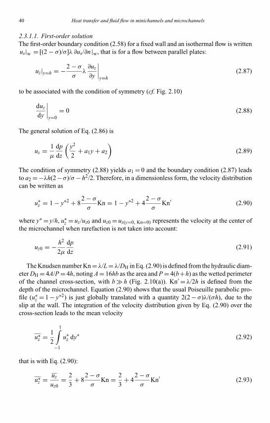
Kandlikar I044527-Ch02.tex 26/10/2005 18: 8 Page 40
40 Heat transfer and fluid flow in minichannels and microchannels
2.3.1.1. First-order solutionThe first-order boundary condition (2.58) for a fixed wall and an isothermal flow is writtenus|w = [(2 − σ)/σ]λ ∂us/∂n |w, that is for a flow between parallel plates:
uz|y=h = −2 − σ
σλ∂uz
∂y
∣∣∣∣y=h
(2.87)
to be associated with the condition of symmetry (cf. Fig. 2.10)
duz
dy
∣∣∣∣y=0
= 0 (2.88)
The general solution of Eq. (2.86) is
uz = 1
µ
dp
dz
(y2
2+ a1y + a2
)(2.89)
The condition of symmetry (2.88) yields a1 = 0 and the boundary condition (2.87) leadsto a2 = −λh(2−σ)/σ− h2/2. Therefore, in a dimensionless form, the velocity distributioncan be written as
u∗z = 1 − y∗2 + 8
2 − σ
σKn = 1 − y∗2 + 4
2 − σ
σKn′ (2.90)
where y∗ = y/h, u∗z = uz/uz0 and uz0 = uz(y=0, Kn=0) represents the velocity at the center of
the microchannel when rarefaction is not taken into account:
uz0 = − h2
2µ
dp
dz(2.91)
The Knudsen number Kn = λ/L = λ/DH in Eq. (2.90) is defined from the hydraulic diam-eter DH = 4A/P = 4h, noting A = 16hb as the area and P = 4(b+h) as the wetted perimeterof the channel cross-section, with b � h (Fig. 2.10(a)). Kn′ = λ/2h is defined from thedepth of the microchannel. Equation (2.90) shows that the usual Poiseuille parabolic pro-file (u∗
z = 1 − y∗2) is just globally translated with a quantity 2(2 − σ)λ/(σh), due to theslip at the wall. The integration of the velocity distribution given by Eq. (2.90) over thecross-section leads to the mean velocity
u∗z = 1
2
1∫−1
u∗z dy∗ (2.92)
that is with Eq. (2.90):
u∗z = uz
uz0= 2
3+ 8
2 − σ
σKn = 2
3+ 4
2 − σ
σKn′ (2.93)

Kandlikar I044527-Ch02.tex 26/10/2005 18: 8 Page 41
Chapter 2. Single-phase gas flow in microchannels 41
We can now calculate the Poiseuille number Po, defined as:
Po = Cf Re (2.94)
where
Cf = τw12ρuz
2(2.95)
is the friction factor that represents a dimensionless value of the average wall shear τw and
Re = ρuzDH
µ(2.96)
is the Reynolds number. The average wall shear is obtained from the force balance
τwP dz = −A dp (2.97)
on a control volume that spans the channel and has an axial extension dz. Therefore,
τw = −DH
4
dp
dz(2.98)
and
Po = −D2H
2µ
dp
dz
1
uz(2.99)
which leads with Eqs. (2.91) and (2.93) to:
PoNS1,plan = 24
1 + 12 2−σσ
Kn= 24
1 + 6 2−σσ
Kn′ (2.100)
Equation (2.100) shows that the Poiseuille number is less than its usual value of 24 for aPoiseuille flow between parallel plates (Shah, 1975), as soon as the Knudsen number isno longer negligible. This result shows that slip at the wall logically reduces friction andconsequently, for a given pressure gradient, the flow rate is increased.
Considering a long microchannel of length l with a pressure pi at the inlet and a pressurepo at the outlet and neglecting the entrance effects, we can deduce from Eq. (2.93) themass flow rate m = ρuz A = puzA/RT , which is independent of z. According to Eq. (2.30),the quantity (Kn p) is constant for an isothermal flow and it can be written as a functionof the outlet conditions: Kn p = Kno po. Therefore, the integration of Eq. (2.93) yields
po∫pi
(2
3p + 8
2 − σ
σKno po
)dp = −2µmRTl
h2A(2.101)

Kandlikar I044527-Ch02.tex 26/10/2005 18: 8 Page 42
42 Heat transfer and fluid flow in minichannels and microchannels
which leads to
mNS1,plan = 2bh3p2o
µRTl
[�2 − 1
3+ 8
2 − σ
σKno(�− 1)
](2.102)
where�= pi/po is the ratio of the inlet over outlet pressures and Kno is the outlet Knudsennumber. The subscript NS1 refers to the Navier–Stokes equations with first-order slip flowboundary conditions. In dimensionless form that compares the actual mass flow rate mwith the mass flow rate mns obtained from a no-slip hypothesis, Eq. (2.102) becomes:
m∗NS1,plan = mNS1,plan
mns,plan= 1 + 24
2 − σ
σ
Kno
�+ 1= 1 + 12
2 − σ
σ
Kn′o
�+ 1(2.103)
The pressure distribution along the z-axis can be found by expressing the conservationof mass flow rate through the channel:
mNS1,plan = 2bh3 p2o
µRTl
[�2 − 1
3+ 8
2 − σ
σKno(�− 1)
]
= 2bh3 p2o
µRT (l − z)
[(p/po)2 − 1
3+ 8
2 − σ
σKno(p/po − 1)
](2.104)
Equation (2.104) shows that the pressure p∗ = p/po is the solution of the polynomial
p∗2 + α1p∗ + α2 + α3z∗ = 0 (2.105)
where z∗ = z/l and
α1 = 242 − σ
σKno α2 = −�(�+ α1) α3 = (�− 1)(�+ 1 + α1) (2.106)
Equation (2.105) is plotted in Fig. 2.11, for an inlet over outlet pressure ratio �= 2.This figure shows that rarefaction and compressibility have opposite effects on the pressuredistribution. Rarefaction effects (characterized by Kn) reduce the curvature in pressuredistribution due to compressibility effects (characterized by Ma).
The first-order mass-flow relation (2.102) accurately predicts the experimental dataavailable in the literature, for moderate outlet Knudsen numbers and typically forKno < 0.03. For higher values of Kno, some deviations appear (cf. Section 2.3.5).
2.3.1.2. Second-order solutionsTherefore, the previous model can be improved to remain accurate for higher Knudsen num-bers. For this purpose, second-order – ϑ(Kn2) – models, based on second-order boundaryconditions or the QHD equations, may be used.
The use of second-order boundary conditions
uz|y=h = −2 − σ
σλ∂uz
∂y
∣∣∣∣y=h
+ A2λ2 ∂
2uz
∂y2
∣∣∣∣y=h
(2.107)

Kandlikar I044527-Ch02.tex 26/10/2005 18: 8 Page 43
Chapter 2. Single-phase gas flow in microchannels 43
1
1.2
1.4
1.6
1.8
2
0 0.2 0.4 0.6 0.8 1z*
p*
Fig. 2.11. Pressure distribution along a plane microchannel. : incompressible flow; �: Kno = 0;+: Kno = 0.05; �: Kno = 0.1.
leads to a velocity distribution
u∗z = 1 − y∗2 + 8
2 − σ
σKn − 32A2 Kn2 = 1 − y∗2 + 4
2 − σ
σKn′ − 8A2 Kn′2 (2.108)
and to a Poiseuille number
PoNS2,plan = 24
1 + 12 2−σσ
Kn − 48 A2 Kn2= 24
1 + 6 2−σσ
Kn′ − 12 A2 Kn′2 (2.109)
It is easy to verify that the mass flow rate is consequently corrected as:
m∗NS2,plan = mNS2,plan
mns,plan= 1 + 24
2 − σ
σ
Kno
�+ 1− 96 A2Kn2
oln�
�2 − 1
= 1 + 122 − σ
σ
Kn′o
�+ 1− 24 A2Kn′2
oln�
�2 − 1(2.110)
It is interesting to note that a close result can also be found keeping the first-orderboundary conditions, but using the QHD equations in place of the NS equations (Elizarovaand Sheretov, 2003). The solution of the momentum equation (2.40), with the expression

Kandlikar I044527-Ch02.tex 26/10/2005 18: 8 Page 44
44 Heat transfer and fluid flow in minichannels and microchannels
(2.53) of the viscous stress tensor and the boundary condition (2.87) yields
m∗QHD1,plan = mQHD1,plan
mns,plan= 1 + 24
2 − σ
σ
Kno
�+ 1+ 96
k22 Sc
Kn2o
ln�
�2 − 1
= 1 + 122 − σ
σ
Kn′o
�+ 1+ 24
k22 Sc
Kn′2o
ln�
�2 − 1(2.111)
Equations (2.110) and (2.111) only differ with their last term. For example, if weconsider the second-order boundary conditions of Deissler, A2 = −9/8 and −96 A2 = 108.This value must be compared with 96/(k2
2 Sc). For an HS model, k2 = 16/5√
2π andSc = 5/6. Therefore, 96/k2
2 Sc = 70, 7. The deviation on the second-order term between thetwo models is then around 42%. But, if we consider the more accurate VSS model, withω= 0.74 for nitrogen under standard conditions (cf. Table 2.2), k2 = 1.064, Sc = 0.746 and96/k2
2 Sc = 114, which corresponds to a deviation of about 5% between the second-orderterms of NS2 and QDH1 models. Of course, this deviation is a function of the gas, thetemperature, the choice of the second-order boundary condition and of the IPL model.
2.3.2. Gas flow in circular microtubes
With the general assumptions of this section, the momentum equation (2.33) in polarcoordinates reduces to
1
r
d
dr
(r
duz
dr
)= 1
µ
dp
dz(2.112)
2.3.2.1. First-order solutionThe first-order boundary condition (2.58) for a non-moving wall and an isothermal flowis now:
uz|r=r2= −2 − σ
σλ∂uz
∂r
∣∣∣∣r=r2
(2.113)
The general solution of Eq. (2.112) is
uz = 1
µ
dp
dz
(r2
4+ c1 ln r + c2
)(2.114)
where c1 = 0 since the velocity has a finite value in r = 0. Using the boundary condition(2.113), we find
c2 = −2 − σ
σλ
r2
2− r2
2
4(2.115)
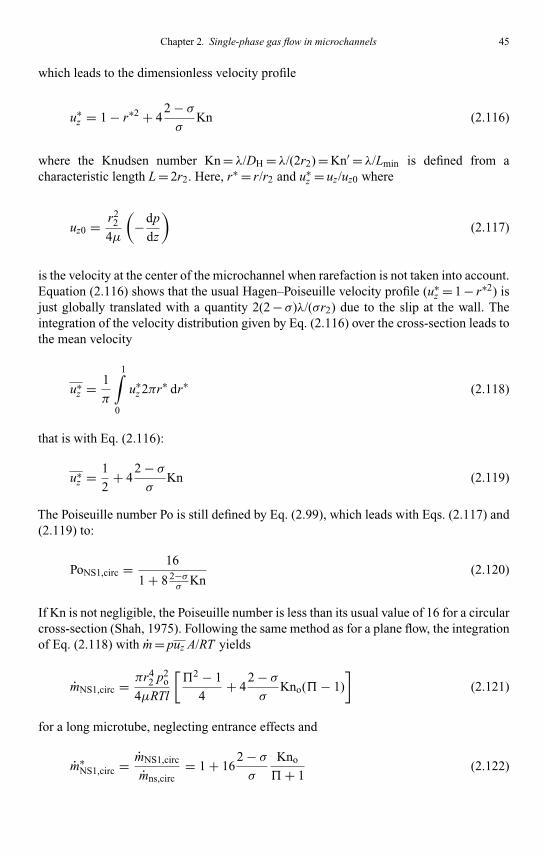
Kandlikar I044527-Ch02.tex 26/10/2005 18: 8 Page 45
Chapter 2. Single-phase gas flow in microchannels 45
which leads to the dimensionless velocity profile
u∗z = 1 − r∗2 + 4
2 − σ
σKn (2.116)
where the Knudsen number Kn = λ/DH = λ/(2r2) = Kn′ = λ/Lmin is defined from acharacteristic length L = 2r2. Here, r∗ = r/r2 and u∗
z = uz/uz0 where
uz0 = r22
4µ
(−dp
dz
)(2.117)
is the velocity at the center of the microchannel when rarefaction is not taken into account.Equation (2.116) shows that the usual Hagen–Poiseuille velocity profile (u∗
z = 1 − r∗2) isjust globally translated with a quantity 2(2 − σ)λ/(σr2) due to the slip at the wall. Theintegration of the velocity distribution given by Eq. (2.116) over the cross-section leads tothe mean velocity
u∗z = 1
π
1∫0
u∗z 2πr∗ dr∗ (2.118)
that is with Eq. (2.116):
u∗z = 1
2+ 4
2 − σ
σKn (2.119)
The Poiseuille number Po is still defined by Eq. (2.99), which leads with Eqs. (2.117) and(2.119) to:
PoNS1,circ = 16
1 + 8 2−σσ
Kn(2.120)
If Kn is not negligible, the Poiseuille number is less than its usual value of 16 for a circularcross-section (Shah, 1975). Following the same method as for a plane flow, the integrationof Eq. (2.118) with m = puz A/RT yields
mNS1,circ = πr42 p2
o
4µRTl
[�2 − 1
4+ 4
2 − σ
σKno(�− 1)
](2.121)
for a long microtube, neglecting entrance effects and
m∗NS1,circ = mNS1,circ
mns,circ= 1 + 16
2 − σ
σ
Kno
�+ 1(2.122)

Kandlikar I044527-Ch02.tex 26/10/2005 18: 8 Page 46
46 Heat transfer and fluid flow in minichannels and microchannels
The pressure distribution p∗ = p/po along the microtube is the solution of the polynomial
p∗2 + β1p∗ + β2 + β3z∗ = 0 (2.123)
where z∗ = z/l and
β1 = 162 − σ
σKno β3 = (�− 1) (�+ 1 + β1) β2 = −1 − β1 − β3 (2.124)
which qualitatively leads to the same conclusions as for a plane flow.
2.3.2.2. Second-order solutionThe first-order solution can easily be extended to second-order boundary conditions,following the same reasoning as in Section 2.3.1.2. We find
u∗z = 1
2+ 4
2 − σ
σKn − 8 A2 Kn2 (2.125)
PoNS2,circ = 16
1 + 8 2−σσ
Kn − 16 A2 Kn2(2.126)
and
m∗NS2,circ = mNS2,circ
mns,circ= 1 + 16
2 − σ
σ
Kno
�+ 1− 32 A2 Kn2
oln�
�2 − 1(2.127)
The problem can also be solved from the QHD equations with first-order boundaryconditions. Lengrand et al. (2004) showed that
m∗QHD1,circ = mQHD1,circ
mns,circ= 1 + 16
2 − σ
σ
Kno
�+ 1+ 32
k22 Sc
Kn2o
ln�
�2 − 1(2.128)
The deviation between the QHD1 and the NS2 models with respect to the second-orderterms are exactly the same as in the case of a plane flow (Section 2.3.1.2).
2.3.3. Gas flow in annular ducts
The solution for the slip-flow of a gas in a circular microduct is easily extensible to thecase of an annular duct (Ebert and Sparrow, 1965). The inner radius r1 and the outer radiusr2 are not necessarily small, but the distance r2 − r1 = DH/2 must be small enough so thatthe flow between the two cylinders is rarefied. The first-order boundary conditions are
uz = 2 − σ
σλ∂uz
∂r
∣∣∣∣r=r1
uz = −2 − σ
σλ∂uz
∂r
∣∣∣∣r=r2
(2.129)

Kandlikar I044527-Ch02.tex 26/10/2005 18: 8 Page 47
Chapter 2. Single-phase gas flow in microchannels 47
The integration of Eq. (2.112) leads to the velocity distribution
u∗z = 1 − r∗2 + 4(1 − r∗
1 )2 − σ
σKn
+ r∗1 (1 − r∗2
1 )(1 + 4 2−σ
σKn) [
2(1 − r∗1 ) 2−σ
σKn − ln r∗
1
]r∗
1 ln r∗1 − 2(1 − r∗2
1 ) 2−σσ
Kn(2.130)
with Kn = Kn′/2 = λ/(2(r2 − r1)) and to its mean value
u∗z = 1
2
[1 + r∗2
1 + 8(1 − r∗1 + r∗2
1 )2 − σ
σKn
+ r∗1 (1 − r∗2
1 )(1 + 4 2−σσ
Kn)2
r∗1 ln r∗
1 − 2(1 − r∗21 ) 2−σ
σKn
](2.131)
Thus, the Poiseuille number takes the form
PoNS1,annu = 16(1 − r∗1 )2
1 + r∗21 + 8(1 − r∗
1 + r∗21 ) 2−σ
σKn + r∗
1 (1−r∗21 )(1+4 2−σ
σKn)2
r∗1 ln r∗
1−2(1−r∗21 ) 2−σ
σKn
(2.132)
which generalizes the expression (2.120) obtained for a circular microtube.
2.3.4. Gas Flow in rectangular microchannels
With the rectangular cross-section defined in Fig. 2.10(c) and the general assumptions ofSection 2.3, the momentum equation takes the form
d2uz
dx2 + d2uz
dy2 = 1
µ
dp
dz(2.133)
In a dimensionless form, the momentum equation can be written
a∗2 d2u∗z
dx∗2 + d2u∗z
dy∗2 = −1 (2.134)
with
x∗ = x
by∗ = y
hu∗
z = uz
− h2
µdpdz
(2.135)
and a∗ = h/b is the aspect ratio of the section with 0< a∗ ≤ 1, if we assume h ≤ b.

Kandlikar I044527-Ch02.tex 26/10/2005 18: 8 Page 48
48 Heat transfer and fluid flow in minichannels and microchannels
2.3.4.1. First-order solutionThe first-order boundary conditions are
u∗z
∣∣y∗=1 = −2 − σ
σ2Kn′ ∂u∗
z
∂y∗
∣∣∣∣y∗=1
(2.136)
u∗z
∣∣x∗=1 = −2 − σ
σ2a∗Kn′ ∂u∗
z
∂x∗
∣∣∣∣x∗=1
(2.137)
with Kn′ = λ/(2h) and the conditions of symmetry
du∗z
dy∗
∣∣∣∣y∗=0
= 0 (2.138)
du∗z
dx∗
∣∣∣∣x∗=0
= 0 (2.139)
Ebert and Sparrow (1965) proposed a solution for the velocity distribution, compatiblewith the condition of symmetry (2.138):
u∗z = −
∞∑i=1
�i(x∗) cos (αiy∗) (2.140)
The eigenvalues αi must verify
αi tan αi = σ
2 − σ
1
2Kn′ (2.141)
in order to be compatible with the boundary condition (2.136) without leading to a trivialvelocity solution. The x∗-dependent �i functions are found by expanding the right-handside of Eq. (2.134), that is unity, in terms of the orthogonal functions cos (αiy∗):
−1 = −∞∑
i=1
�i cos (αiy∗) = −
∞∑i=1
2 sin αi
αi + sin αi cosαicos (αiy
∗) (2.142)
Therefore, to verify the momentum equation (2.134), the functions �i must obey
d2�i
dx∗2 −(αi
a∗)2�i − �i
a∗2 = 0 (2.143)
The solution of Eq. (2.143), with the conditions (2.137)–(2.139) and using Eq. (2.141), is
�i = −�i
α2i
1 −
cosh(αix∗a∗)
cosh(αia∗)+ 2Kn′ 2−σ
σαi sinh
(αia∗) (2.144)

Kandlikar I044527-Ch02.tex 26/10/2005 18: 8 Page 49
Chapter 2. Single-phase gas flow in microchannels 49
Consequently, the velocity distribution is given by Eq. (2.140). This solution is givenas a function of a Knudsen number Kn′ = λ/(2h) based on the channel depth, but it canalso be expressed as a function of the previous Knudsen number Kn = λ/DH based on thehydraulic diameter by using the relation
2Kn = Kn′(1 + a∗) (2.145)
In the special case of a square section, for which a∗ = 1, both Knudsen numbers Knand Kn′ are identical.
2.3.4.2. Second-order solutionThe above solution from Ebert et Sparrow was improved by Aubert and Colin (2001),in order to be more accurate for higher Knudsen numbers. This model is based on thesecond-order boundary conditions proposed by Deissler (1964):
uz|y=h = −2 − σ
σλ∂uz
∂y
∣∣∣∣y=h
− 9
16λ2
(2∂2uz
∂y2
∣∣∣∣y=h
+ ∂2uz
∂x2
∣∣∣∣y=h
+ ∂2uz
∂z2
∣∣∣∣y=h
)(2.146)
and
uz|x=b = −2 − σ
σλ∂uz
∂x
∣∣∣∣x=b
− 9
16λ2(
2∂2uz
∂x2
∣∣∣∣x=b
+ ∂2uz
∂y2
∣∣∣∣x=b
+ ∂2uz
∂z2
∣∣∣∣x=b
)(2.147)
This choice of Deissler boundary conditions, rather than other second-order formula-tions such as the ones proposed in Section 2.2.3.3, is due to the physical approach proposedby Deissler. The above equations are obtained from a three dimensional local momentumbalance at the wall and the shear stress satisfies the definition of a Newtonian fluid used inthe Navier–Stokes equations.
In Eqs. (2.146) and (2.147), the term ∂2uz/∂z2 vanishes according to the continuityequation, which reduces to ∂uz/∂z = 0 for a locally fully developed flow. Finally, using themomentum equation (2.134), these equations may be written in a non-dimensional formas follows:
u∗z
∣∣y∗=1 = −2 − σ
σ2Kn′ ∂u∗
z
∂y∗
∣∣∣∣y∗=1
− 9
4Kn′2
(∂2u∗
z
∂y∗2
∣∣∣∣y∗=1
− 1
)(2.148)
and
u∗z
∣∣x∗=1 = −2 − σ
σ2a∗Kn′ ∂u∗
z
∂x∗
∣∣∣∣x∗=1
− 9
4Kn′2
(a∗2 ∂
2u∗z
∂x∗2
∣∣∣∣x∗=1
− 1)
(2.149)
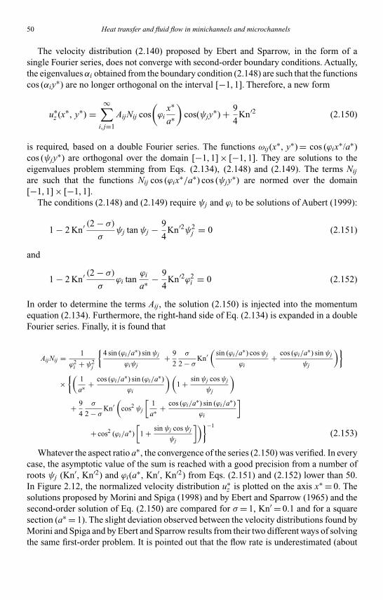
Kandlikar I044527-Ch02.tex 26/10/2005 18: 8 Page 50
50 Heat transfer and fluid flow in minichannels and microchannels
The velocity distribution (2.140) proposed by Ebert and Sparrow, in the form of asingle Fourier series, does not converge with second-order boundary conditions. Actually,the eigenvalues αi obtained from the boundary condition (2.148) are such that the functionscos (αiy∗) are no longer orthogonal on the interval [−1, 1]. Therefore, a new form
u∗z (x∗, y∗) =
∞∑i, j=1
AijNij cos(ϕi
x∗
a∗
)cos(ψjy
∗) + 9
4Kn′2 (2.150)
is required, based on a double Fourier series. The functions ωij(x∗, y∗) = cos (ϕix∗/a∗)cos (ψjy∗) are orthogonal over the domain [−1, 1] × [−1, 1]. They are solutions to theeigenvalues problem stemming from Eqs. (2.134), (2.148) and (2.149). The terms Nij
are such that the functions Nij cos (ϕix∗/a∗) cos (ψjy∗) are normed over the domain[−1, 1] × [−1, 1].
The conditions (2.148) and (2.149) require ψj and ϕi to be solutions of Aubert (1999):
1 − 2 Kn′ (2 − σ)
σψj tanψj − 9
4Kn′2ψ2
j = 0 (2.151)
and
1 − 2 Kn′ (2 − σ)
σϕi tan
ϕi
a∗ − 9
4Kn′2ϕ2
i = 0 (2.152)
In order to determine the terms Aij , the solution (2.150) is injected into the momentumequation (2.134). Furthermore, the right-hand side of Eq. (2.134) is expanded in a doubleFourier series. Finally, it is found that
AijNij = 1
ϕ2i + ψ2
j
{4 sin (ϕi/a∗) sinψj
ϕiψj+ 9
2
σ
2 − σKn′
(sin (ϕi/a∗) cosψj
ϕi+ cos (ϕi/a∗) sinψj
ψj
)}
×{(
1
a∗ + cos (ϕi/a∗) sin (ϕi/a∗)
ϕi
)(1 + sinψj cosψj
ψj
)
+ 9
4
σ
2 − σKn′
(cos2 ψj
[1
a∗ + cos (ϕi/a∗) sin (ϕi/a∗)
ϕi
]
+ cos2 (ϕi/a∗)[
1 + sinψj cosψj
ψj
])}−1
(2.153)
Whatever the aspect ratio a∗, the convergence of the series (2.150) was verified. In everycase, the asymptotic value of the sum is reached with a good precision from a number ofroots ψj (Kn′, Kn′2) and ϕi(a∗, Kn′, Kn′2) from Eqs. (2.151) and (2.152) lower than 50.In Figure 2.12, the normalized velocity distribution u∗
z is plotted on the axis x∗ = 0. Thesolutions proposed by Morini and Spiga (1998) and by Ebert and Sparrow (1965) and thesecond-order solution of Eq. (2.150) are compared for σ= 1, Kn′ = 0.1 and for a squaresection (a∗ = 1). The slight deviation observed between the velocity distributions found byMorini and Spiga and by Ebert and Sparrow results from their two different ways of solvingthe same first-order problem. It is pointed out that the flow rate is underestimated (about

Kandlikar I044527-Ch02.tex 26/10/2005 18: 8 Page 51
Chapter 2. Single-phase gas flow in microchannels 51
0
0.1
0.2
0.3
0.4
0.5
0 0.2 0.4 0.6 0.8 1
12
3
y ∗
u z∗
Fig. 2.12. Normalized velocity distribution in a square cross-section with diffuse reflection at the wall forKn′ = 0.1. 1: second-order model; 2: first-order model (Ebert and Sparrow, 1965); 3: first-order model (Moriniand Spiga, 1998).
10% in the case of Fig. 2.12) when the second-order terms are not taken into account.Moreover, it is verified that the velocity distribution obtained with a second-order modelcannot be deduced from a simple translation of the first-order velocity distribution.
The mass flow rate through the cross-section (�) is m = ∫∫(�)
ρuz dx dy, that is with
Eqs. (2.135) and (2.150):
mNS2,rect = −ρh2
µ
dp
dz
4h2
a∗
∞∑
i, j=1
AijNija∗ sin (ϕi/a∗) sinψj
ϕiψj+ 9
4Kn′2
(2.154)
In order to obtain m as a function of the inlet pressure pi and the outlet pressure poof a long rectangular microchannel of length l, Eq. (2.154) must be integrated alongthe microchannel. For an isothermal flow and known geometric dimensions, the Knud-sen number only depends on the pressure p(z). Therefore, the solutions ϕi and ψj ofEqs. (2.151) and (2.152) depend on the position along the z-axis. The bracketed term ofEq. (2.154) can be precisely fitted by a polynomial function a1 + a2Kn′ + a3Kn′2, wherea1, a2 and a3 are coefficients depending on the aspect ratio a∗ of the cross-section and onthe momentum accommodation coefficient σ for a2 and a3. Thus,
mNS2,rect = − 4ph4
a∗RTµ
dp
dz[a1 + a2Kn′ + a3Kn′2] (2.155)
Some numerical values of the coefficients a1, a2 and a3, obtained with a least squaresfitting method from values calculated using Eq. (2.154) for Kn′ ∈ [0; 1], are given in
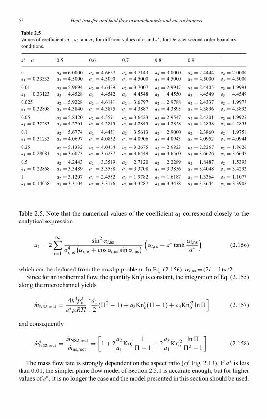
Kandlikar I044527-Ch02.tex 26/10/2005 18: 8 Page 52
52 Heat transfer and fluid flow in minichannels and microchannels
Table 2.5Values of coefficients a1, a2 and a3 for different values of σ and a∗, for Deissler second-order boundaryconditions.
a∗ σ 0.5 0.6 0.7 0.8 0.9 1
0 a2 = 6.0000 a2 = 4.6667 a2 = 3.7143 a2 = 3.0000 a2 = 2.4444 a2 = 2.0000a1 = 0.33333 a3 = 4.5000 a3 = 4.5000 a3 = 4.5000 a3 = 4.5000 a3 = 4.5000 a3 = 4.5000
0.01 a2 = 5.9694 a2 = 4.6459 a2 = 3.7007 a2 = 2.9917 a2 = 2.4405 a2 = 1.9993a1 = 0.33123 a3 = 4.4528 a3 = 4.4542 a3 = 4.4548 a3 = 4.4550 a3 = 4.4549 a3 = 4.4549
0.025 a2 = 5.9228 a2 = 4.6141 a2 = 3.6797 a2 = 2.9788 a2 = 2.4337 a2 = 1.9977a1 = 0.32808 a3 = 4.3840 a3 = 4.3875 a3 = 4.3887 a3 = 4.3895 a3 = 4.3896 a3 = 4.3892
0.05 a2 = 5.8420 a2 = 4.5591 a2 = 3.6423 a2 = 2.9547 a2 = 2.4201 a2 = 1.9925a1 = 0.32283 a3 = 4.2761 a3 = 4.2813 a3 = 4.2843 a3 = 4.2858 a3 = 4.2858 a3 = 4.2853
0.1 a2 = 5.6774 a2 = 4.4431 a2 = 3.5613 a2 = 2.9000 a2 = 2.3860 a2 = 1.9751a1 = 0.31233 a3 = 4.0697 a3 = 4.0832 a3 = 4.0906 a3 = 4.0943 a3 = 4.0952 a3 = 4.0944
0.25 a2 = 5.1332 a2 = 4.0464 a2 = 3.2675 a2 = 2.6823 a2 = 2.2267 a2 = 1.8626a1 = 0.28081 a3 = 3.6073 a3 = 3.6287 a3 = 3.6449 a3 = 3.6560 a3 = 3.6626 a3 = 3.6647
0.5 a2 = 4.2443 a2 = 3.3519 a2 = 2.7120 a2 = 2.2289 a2 = 1.8487 a2 = 1.5395a1 = 0.22868 a3 = 3.3489 a3 = 3.3588 a3 = 3.3708 a3 = 3.3856 a3 = 3.4048 a3 = 3.4292
1 a2 = 3.1207 a2 = 2.4552 a2 = 1.9782 a2 = 1.6187 a2 = 1.3364 a2 = 1.1077a1 = 0.14058 a3 = 3.3104 a3 = 3.3176 a3 = 3.3287 a3 = 3.3438 a3 = 3.3644 a3 = 3.3908
Table 2.5. Note that the numerical values of the coefficient a1 correspond closely to theanalytical expression
a1 = 2∞∑
i=1
sin2 αi,ns
α4i,ns
(αi,ns + cosαi,ns sin αi,ns
) (αi,ns − a∗ tanhαi,ns
a∗)
(2.156)
which can be deduced from the no-slip problem. In Eq. (2.156), αi,ns = (2i − 1)π/2.Since for an isothermal flow, the quantity Kn′p is constant, the integration of Eq. (2.155)
along the microchannel yields
mNS2,rect = 4h4p2o
a∗µRTl
[a1
2(�2 − 1) + a2Kn′
o(�− 1) + a3Kn′2o ln�
](2.157)
and consequently
m∗NS2,rect = mNS2,rect
mns,rect=[
1 + 2a2
a1Kn′
o1
�+ 1+ 2
a3
a1Kn′2
oln�
�2 − 1
](2.158)
The mass flow rate is strongly dependent on the aspect ratio (cf. Fig. 2.13). If a∗ is lessthan 0.01, the simpler plane flow model of Section 2.3.1 is accurate enough, but for highervalues of a∗, it is no longer the case and the model presented in this section should be used.
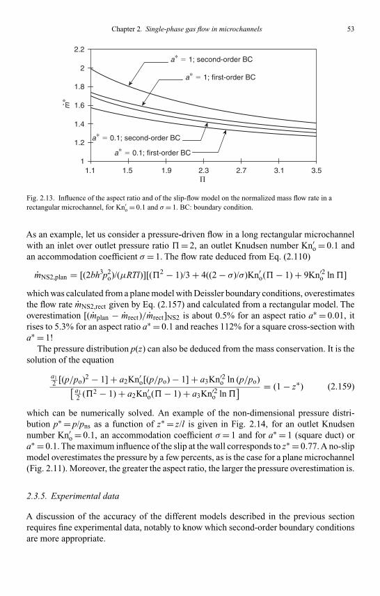
Kandlikar I044527-Ch02.tex 26/10/2005 18: 8 Page 53
Chapter 2. Single-phase gas flow in microchannels 53
1
1.2
1.4
1.6
1.8
2
2.2
1.1 1.5 1.9 2.3 2.7 3.1 3.5
m∗
�
a∗ � 1; second-order BC
a∗ � 0.1; second-order BC
a∗ � 1; first-order BC
a∗ � 0.1; first-order BC
Fig. 2.13. Influence of the aspect ratio and of the slip-flow model on the normalized mass flow rate in arectangular microchannel, for Kn′
o = 0.1 and σ= 1. BC: boundary condition.
As an example, let us consider a pressure-driven flow in a long rectangular microchannelwith an inlet over outlet pressure ratio �= 2, an outlet Knudsen number Kn′
o = 0.1 andan accommodation coefficient σ= 1. The flow rate deduced from Eq. (2.110)
mNS2,plan = [(2bh3p2o)/(µRTl)][(�2 − 1)/3 + 4((2 − σ)/σ)Kn′
o(�− 1) + 9Kn′2o ln�]
which was calculated from a plane model with Deissler boundary conditions, overestimatesthe flow rate mNS2,rect given by Eq. (2.157) and calculated from a rectangular model. Theoverestimation [(mplan − mrect)/mrect]NS2 is about 0.5% for an aspect ratio a∗ = 0.01, itrises to 5.3% for an aspect ratio a∗ = 0.1 and reaches 112% for a square cross-section witha∗ = 1!
The pressure distribution p(z) can also be deduced from the mass conservation. It is thesolution of the equation
a12 [(p/po)2 − 1] + a2Kn′
o[(p/po) − 1] + a3Kn′2o ln (p/po)[ a1
2 (�2 − 1) + a2Kn′o(�− 1) + a3Kn′2
o ln�] = (1 − z∗) (2.159)
which can be numerically solved. An example of the non-dimensional pressure distri-bution p∗ = p/pns as a function of z∗ = z/l is given in Fig. 2.14, for an outlet Knudsennumber Kn′
o = 0.1, an accommodation coefficient σ= 1 and for a∗ = 1 (square duct) ora∗ = 0.1. The maximum influence of the slip at the wall corresponds to z∗ = 0.77. A no-slipmodel overestimates the pressure by a few percents, as is the case for a plane microchannel(Fig. 2.11). Moreover, the greater the aspect ratio, the larger the pressure overestimation is.
2.3.5. Experimental data
A discussion of the accuracy of the different models described in the previous sectionrequires fine experimental data, notably to know which second-order boundary conditionsare more appropriate.

Kandlikar I044527-Ch02.tex 26/10/2005 18: 8 Page 54
54 Heat transfer and fluid flow in minichannels and microchannels
0.95
0.96
0.97
0.98
0.99
1
0
p∗
0.2 0.4 0.6 0.8 1z ∗
a∗ � 0.1; second-order BC
a∗ � 1; second-order BC
a∗ � 0.1; first-order BC
a∗ � 1; first-order BC
Fig. 2.14. Influence of the aspect ratio and of the slip-flow model on the normalized pressure distribution alonga rectangular microchannel, for Kn′
o = 0.1 and σ= 1. BC: boundary condition.
2.3.5.1. Experimental setups for flow rate measurementsFew experimental setups are described in the literature. The first techniques used to pro-vide experimental data of gas flow rates in a microchannel were proposed by Arkilic et al.(1994) or by Pong et al. (1994). They both used accumulation techniques: the gas flowingthrough the microchannel accumulates in a reservoir, resulting in either a change in pres-sure (constant-volume technique) or a change in volume (constant-pressure technique).Actually, this method is limited because the tiny mass flows are very difficult to measureaccurately using a single tank. In particular very small changes in temperature can over-whelm the mass flow measurement due to thermal expansion of the gas. To overcome thisdifficulty, a differential technique was used afterwards (Arkilic et al., 1998). The systemis schematically represented in Fig. 2.15. Gas flows through the test microchannel andinto the accumulation tank A. The mass flow through the system can be inferred from ameasurement of the differential pressure between the accumulation tank A and a refer-ence tank B. This arrangement is very insensitive to temperature fluctuations and allowsaccurate measurements of mass flow rates, with a sensitivity announced to be as low as7 × 10−5 kg/s.
Another experimental setup was designed by Lalonde (2001) for the measurement ofgaseous microflow rates under controlled temperature and pressure conditions, in the range10−7 to 10−13 m3/s. Its principle is based on the tracking of a drop meniscus in a calibratedpipette connected in series with the microchannel. Its main advantage, compared to othersimilar setups presented in the literature (Shih et al., 1996; Zohar et al., 2002; Maurer et al.,2003), is the simultaneous measurement of the flow rate both upstream and downstream ofthe microchannel (Fig. 2.16). The inlet and the outlet pressures can both be independentlytuned. The volume flow rate is measured by means of opto-electronical sensors that detectthe passage of the two menisci of a liquid drop injected into the calibrated pipettes connectedupstream and downstream of the microchannel.
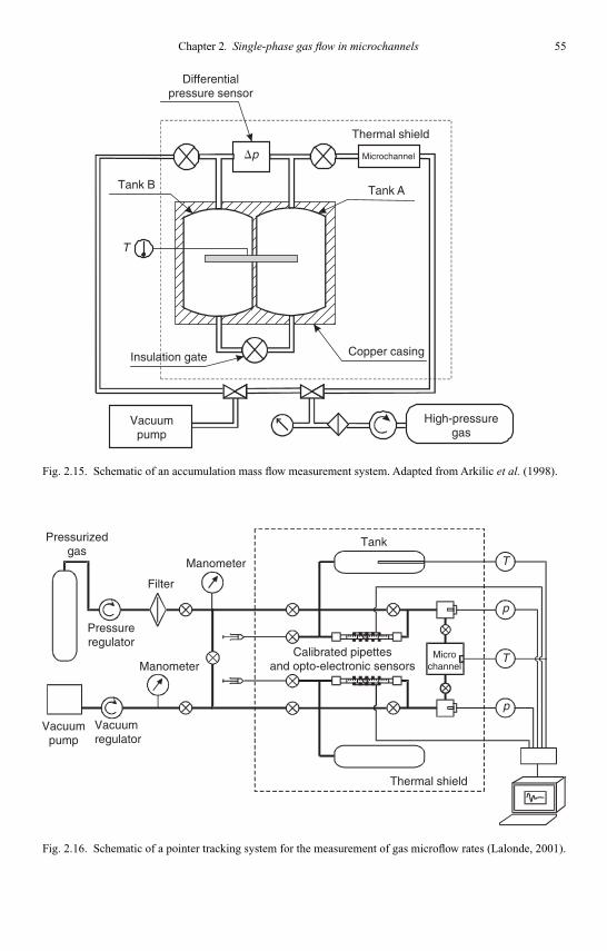
Kandlikar I044527-Ch02.tex 26/10/2005 18: 8 Page 55
Chapter 2. Single-phase gas flow in microchannels 55
Microchannel�p
Vacuumpump
Copper casing
T
Differentialpressure sensor
Insulation gate
High-pressuregas
Tank B Tank A
Thermal shield
Fig. 2.15. Schematic of an accumulation mass flow measurement system. Adapted from Arkilic et al. (1998).
Calibrated pipettesand opto-electronic sensors
Tank
Manometer
Manometer
Pressurizedgas
Pressureregulator
Filter
Vacuumregulator
Vacuumpump
T
T
p
p
Thermal shield
Microchannel
Fig. 2.16. Schematic of a pointer tracking system for the measurement of gas microflow rates (Lalonde, 2001).
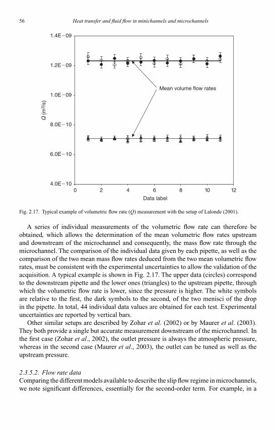
Kandlikar I044527-Ch02.tex 26/10/2005 18: 8 Page 56
56 Heat transfer and fluid flow in minichannels and microchannels
4.0E�10
6.0E�10
8.0E�10
1.0E�09
1.2E�09
1.4E�09
0 2 4 6 8 10 12
Data label
Q (
m3 /
s)
Mean volume flow rates
Fig. 2.17. Typical example of volumetric flow rate (Q) measurement with the setup of Lalonde (2001).
A series of individual measurements of the volumetric flow rate can therefore beobtained, which allows the determination of the mean volumetric flow rates upstreamand downstream of the microchannel and consequently, the mass flow rate through themicrochannel. The comparison of the individual data given by each pipette, as well as thecomparison of the two mean mass flow rates deduced from the two mean volumetric flowrates, must be consistent with the experimental uncertainties to allow the validation of theacquisition. A typical example is shown in Fig. 2.17. The upper data (circles) correspondto the downstream pipette and the lower ones (triangles) to the upstream pipette, throughwhich the volumetric flow rate is lower, since the pressure is higher. The white symbolsare relative to the first, the dark symbols to the second, of the two menisci of the dropin the pipette. In total, 44 individual data values are obtained for each test. Experimentaluncertainties are reported by vertical bars.
Other similar setups are described by Zohar et al. (2002) or by Maurer et al. (2003).They both provide a single but accurate measurement downstream of the microchannel. Inthe first case (Zohar et al., 2002), the outlet pressure is always the atmospheric pressure,whereas in the second case (Maurer et al., 2003), the outlet can be tuned as well as theupstream pressure.
2.3.5.2. Flow rate dataComparing the different models available to describe the slip flow regime in microchannels,we note significant differences, essentially for the second-order term. For example, in a

Kandlikar I044527-Ch02.tex 26/10/2005 18: 8 Page 57
Chapter 2. Single-phase gas flow in microchannels 57
plane flow between parallel plates, the mass flow rate predicted by Eq. (2.110) depends onthe choice of the second-order boundary condition. According to the value of the coefficientA2 (see Table 2.3), the calculated mass flow rate may vary significantly. Moreover, somemodels generally based on a simple mathematical extension of Maxwell’s condition (2.58)and for which A2 > 0 predict a decrease of the slip compared to the first-order model. Whileother models, for which A2 < 0, predict an increase of the slip. It is also interesting to testthe accuracy of a QHD model, which does not involve second-order boundary conditions,but is second-order Knudsen number dependent (cf. Eq. (2.111)).
The increase of the slip due to second-order terms was first confirmed by Lalonde(2001), who measured the flow rate of helium and nitrogen in rectangular microchannelsand showed that for outlet Knudsen numbers Kn′
o,M higher than 0.05, a first-order modelunderestimates the slip. For the comparison of the experimental flow rate data with thepredictions from the different models presented above, the sources of error or uncertaintymust be considered. They can globally be divided into three classes:
(1) The uncertainties inherent to the fluid properties (density, viscosity, dissolved air, etc.)and to their dependence toward the experimental parameters (temperature, pressure).One can also note that some properties such as the momentum accommodationcoefficient, σ, depend both on the fluid and the wall.
(2) The uncertainties relative to the microchannel geometrical characteristics (dimensionsof the section, roughness, etc.) and to their dispersion.
(3) The uncertainties due to the flow rate measurement (metrology, leakage, operatingconditions, etc.).
Most of these uncertainties can be limited within an acceptable precision. This is gen-erally not the case for the measurement of the cross-section dimensions. When thesedimensions are of the order of 1 µm, the measures obtained by different means (profilome-ter, optical microscope, SEM) that require preliminary calibration can differ notably: up toabout 5% for the width and about 10% for the depth (Anduze, 2000). Therefore, the data arehardly exploitable, since the hydraulic diameter plays a part to the power of 4 in the calcu-lation of the flow rate. Also, an inaccuracy of only 10 nm when measuring a depth of 1 µmleads to an error of 4% in the estimation of the flow rate. The second parameter that can posea problem is the accommodation coefficient σ, the value of which is not usually well known.
In order to avoid interpretation errors due to these two mains sources of uncertainty,the idea is to compare among themselves data measured on a same microchannel, in aKnudsen number range that covers at least two of the following regimes:
(1) In the little rarefied regime, differences between the flow rates predicted by the no-slip(ns), the NS1 and the NS2 models are negligible, of the order of the experimentaluncertainties. The value of σ consequently does not play any significant role.
(2) In the lightly rarefied regime, the difference between NS1 and NS2 models remainsnegligible, but the difference with the ns model is now significant. The influence of theaccommodation coefficientσ may also become significant for the higher values of Kn′
o.(3) In the moderately rarefied regime, the ns, NS1 and NS2 models predict significantly
different flow rates, and σ is now a very sensitive parameter.

Kandlikar I044527-Ch02.tex 26/10/2005 18: 8 Page 58
58 Heat transfer and fluid flow in minichannels and microchannels
2h � 0.545 µmMicrochannel no.4
a∗ � 0.011
2h � 1.16 µmMicrochannel no.3
a∗ � 0.055
2h � 1.88 µmMicrochannel no.2
a∗ � 0.089
Littl
e ra
refie
d
Ligh
tly r
aref
ied
Mod
erat
ely
rare
fied
2h � 4.48 µmMicrochannel no.1
a∗ � 0.087
0.001 0.01 0.1Kn�o,VSS
1
Fig. 2.18. Knudsen number ranges covered by a series of rectangular microchannels tested by Lalonde (2001),the right part of the rectangles corresponds to the outlet Knudsen number values.
Figure 2.18 represents these regimes with a series of microchannels experimentallystudied by Lalonde (Colin et al., 2004).
The microchannel no.1, with a measured depth 2h = 4.48 µm, allows a check of thetransition from ns to NS1 models. First, the flow rate is measured for low values of the outletKnudsen number Kn′
o, that is for high values of Po. For Kn′o,VSS = 0.007, the differences
between the flow rates predicted from the NS1 and NS2 models are negligible, whatever thevalue of the accommodation coefficient σ and the deviation with the ns model remains ofthe order of the experimental uncertainties. The depth 2h kept for the simulation is adjustedto 4.48 µm – exactly the measured value in that case – for a good correlation between theexperimental data and the NS1 or NS2 model. Then, rarefaction is increased, by decreasingthe outlet pressure; the difference between ns and NS1 or NS2 models becomes significantand the experimental data are in very good agreement with the slip flow models. Theinfluence of σ is still negligible as is the deviation between NS1 and NS2 models.
The microchannels nos.3 and 4 allow a check of the transition from NS1 to NS2 mod-els. As an illustration, Fig. 2.19 shows some flow rate data relative to the microchannelno.3, whose measured depth is 2h = 1.15 µm. The depth for the simulation is adjusted to1.16 µm, that is 0.01 µm more than the measured value, from data at low values of Kn′
o,for which both NS1 and NS2 models accurately predict the experimental flow rates. Anincrease of the rarefaction leads to a deviation between these two models. The agreementbetween the experimental data and the NS2 model is good, whatever the gas – nitrogen(Fig. 2.19(b)) or helium (Fig. 2.19(c)) – with σ= 0.93. The rarefaction is increased evenmore and the difference between NS1 and NS2 models becomes very significant (Fig.2.19(d)). The experiment shows the validity of the second-order slip flow model withKnudsen numbers higher than 0.2. This observation is confirmed with the microchannelno.4, up to Knudsen numbers around 0.25.

Kandlikar I044527-Ch02.tex 26/10/2005 18: 8 Page 59
Chapter 2. Single-phase gas flow in microchannels 59
0
4E�12
8E�12
1.2E�11
1.6E�11
2E�11
1.1 1.2 1.3 1.4 1.5 1.6 1.7 1.8 1.9
�
�
NS1 and NS2 (s � 1)
NS2 (s � 1)
NS1 (s � 1)
NS2 (s � 0.93)
NS2 (s � 0.93)
ns
m (
kg/s
)m
(kg
/s)
(a)
5.0E�13
1.0E�12
1.5E�12
2.0E�12
2.5E�12
3.0E�12
3.5E�12
1.3 1.4 1.5 1.6 1.7 1.8 1.9 2.0
ns
(b)
Fig. 2.19. Theoretical and experimental flow rates for a rectangular microchannel. 2 h = 1.16 µm,2b = 21 µm, l = 5000 µm, T = 294.2 K. (a) Gas: N2, po = 1.9 × 10⁵ Pa, Kn′
o,VSS = 2.5 × 10⁻²; (b) gas: N2,po = 0.65 × 10⁵Pa, Kn′
o,VSS = 7.3 × 10⁻².
For nitrogen and helium flows, an attempt to summarize the results obtained with themicrochannels nos.2, 3 and 4 is shown in Fig. 2.20. The dimensionless flow rate 1/m∗,little sensitive to the aspect ratio a∗, is plotted in function of Kn′
o,M, for an inlet over outletpressure ratio �= 1.8. Up to Kn′
o,M = 0.05, the first-order (NS1) and the second-order(NS2) slip flow models predict the same flow rate. For higher values of Kn′
o, the deviationis significant and the experimental data are in very good agreement with the NS2 model,
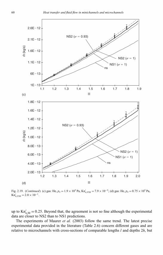
Kandlikar I044527-Ch02.tex 26/10/2005 18: 8 Page 60
60 Heat transfer and fluid flow in minichannels and microchannels
1E�13
6E�13
1.1E�12
1.6E�12
2.1E�12
2.6E�12
1.1 1.2 1.3 1.4 1.5 1.6 1.7 1.8 1.9
ns
ns
(c)
2.0E�13
4.0E�13
6.0E�13
8.0E�13
1.0E�12
1.2E�12
1.4E�12
1.6E�12
1.8E�12
1.2 1.3 1.4 1.5 1.6 1.7 1.8 1.9 2.0
m (
kg/s
)m
(kg
/s)
(d)
NS2 (s � 0.93)
NS2 (s � 0.93)
NS2 (s � 1)
NS1 (s � 1)
NS2 (s � 1)
NS1 (s � 1)
�
�
Fig. 2.19. (Continued) (c) gas: He, po = 1.9 × 10⁵ Pa, Kn′o,VSS = 7.9 × 10⁻²; (d) gas: He, po = 0.75 × 10⁵ Pa,
Kn′o,VSS = 2.0 × 10⁻¹.
up to Kn′o,M = 0.25. Beyond that, the agreement is not so fine although the experimental
data are closer to NS2 than to NS1 predictions.The experiments of Maurer et al. (2003) follow the same trend. The latest precise
experimental data provided in the literature (Table 2.6) concern different gases and arerelative to microchannels with cross-sections of comparable lengths l and depths 2h, but
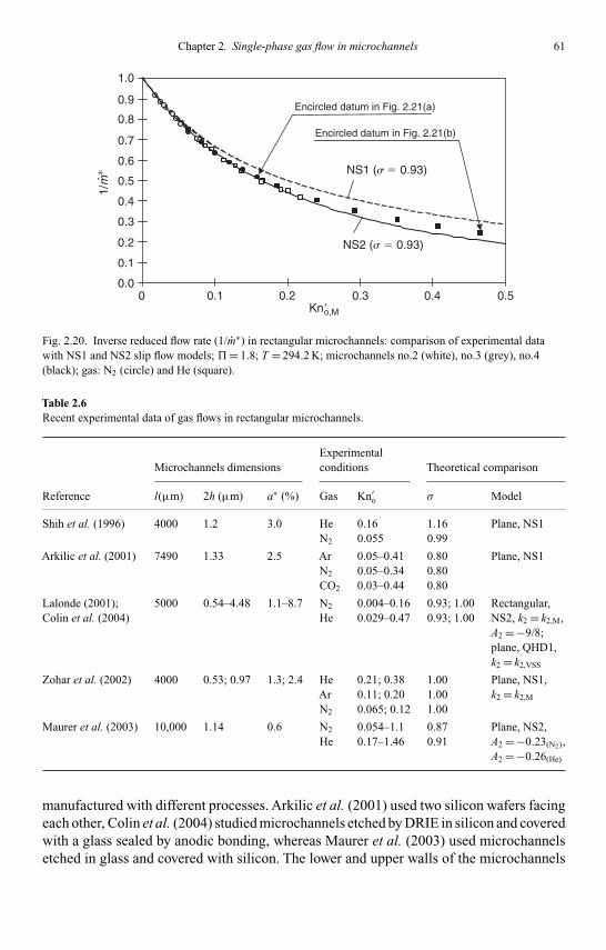
Kandlikar I044527-Ch02.tex 26/10/2005 18: 8 Page 61
Chapter 2. Single-phase gas flow in microchannels 61
1.0
Encircled datum in Fig. 2.21(a)
Encircled datum in Fig. 2.21(b)
0.9
0.8
0.7
0.6
0.5
0.4
0.3
0.2
0.1
0.00 0.1 0.2 0.3 0.4 0.5
NS1 (s � 0.93)
NS2 (s � 0.93)
Kn�o,M
1/m
∗
Fig. 2.20. Inverse reduced flow rate (1/m∗) in rectangular microchannels: comparison of experimental datawith NS1 and NS2 slip flow models; �= 1.8; T = 294.2 K; microchannels no.2 (white), no.3 (grey), no.4(black); gas: N2 (circle) and He (square).
Table 2.6Recent experimental data of gas flows in rectangular microchannels.
ExperimentalMicrochannels dimensions conditions Theoretical comparison
Reference l(µm) 2h (µm) a∗ (%) Gas Kn′o σ Model
Shih et al. (1996) 4000 1.2 3.0 He 0.16 1.16 Plane, NS1N2 0.055 0.99
Arkilic et al. (2001) 7490 1.33 2.5 Ar 0.05–0.41 0.80 Plane, NS1N2 0.05–0.34 0.80CO2 0.03–0.44 0.80
Lalonde (2001); 5000 0.54–4.48 1.1–8.7 N2 0.004–0.16 0.93; 1.00 Rectangular,Colin et al. (2004) He 0.029–0.47 0.93; 1.00 NS2, k2 = k2,M,
A2 = −9/8;plane, QHD1,k2 = k2,VSS
Zohar et al. (2002) 4000 0.53; 0.97 1.3; 2.4 He 0.21; 0.38 1.00 Plane, NS1,Ar 0.11; 0.20 1.00 k2 = k2,M
N2 0.065; 0.12 1.00
Maurer et al. (2003) 10,000 1.14 0.6 N2 0.054–1.1 0.87 Plane, NS2,He 0.17–1.46 0.91 A2 = −0.23(N2),
A2 = −0.26(He)
manufactured with different processes. Arkilic et al. (2001) used two silicon wafers facingeach other, Colin et al. (2004) studied microchannels etched by DRIE in silicon and coveredwith a glass sealed by anodic bonding, whereas Maurer et al. (2003) used microchannelsetched in glass and covered with silicon. The lower and upper walls of the microchannels

Kandlikar I044527-Ch02.tex 26/10/2005 18: 8 Page 62
62 Heat transfer and fluid flow in minichannels and microchannels
fabricated by Zohar et al. (2002) were obtained by deposition of low-stress silicon nitridelayers on a silicon wafer.
A smart comparison of the data provided by these authors is also tricky, since the aspectratios a∗ of the sections are different from one study to another. The two latter studies(Maurer et al., 2003; Colin et al., 2004) confirm that an adequate slip flow model based onsecond-order boundary conditions can be precise for high Knudsen numbers that usuallyapply to the transition regime.
The experimental data from Lalonde have also been compared (Colin et al., 2003) to themass flow predicted by a QHD model with first-order boundary conditions (QHD1). For themicrochannel no.4, with a low aspect ratio a∗ = 0.011, the plane assumption is acceptableand Eq. (2.111) is valid. Figure 2.21 shows that the QHD1 model could be accuratefor Knudsen numbers higher than the NS2 model, but with a different accommodationcoefficient, σ= 1, both for nitrogen and helium. Actually, the analysis of this result shouldbe qualified. For this comparison, the mean free path was calculated using the formulagiven by Maxwell (k2,M = √
π/2) for the NS2 as well as for the QHD1 simulations, butthe Schmidt value (0.74 for nitrogen and 0.77 for helium) used for the QHD1 simulationis very close to the one obtained from a VSS model, that is given by Eq. (2.46). Anothercomparison of the QHD1 model with the data of Lalonde is proposed in Elizarova andSheretov (2003), using k2,VSS calculated from the VSS model (cf. Table 2.1). In this case,the better fit is found for σ= 1 for helium and σ= 0.93 for nitrogen.
To conclude, it is clear that the NS2 or QHD1 models improve the accuracy of the NS1model, but further studies that include smart experimental data are necessary to dissociatethe roles of the accommodation coefficient, the collision model and the slip flow model.
2.3.5.3. Pressure dataPressure measurements along a microchannel have been successfully performed by differ-ent groups (Liu et al., 1995; Lee et al., 2002; Zohar et al., 2002; Jang and Wereley, 2004),using integrated pressure microsensors connected to the microchannels via capillary con-nections (Fig. 2.22). These experiments confirm the theoretical pressure distribution shownin Fig. 2.11.
2.3.5.4. Flow visualizationAlthough micro-particle image velocimetry (micro-PIV) has been widely used to visu-alize liquid microflows for several years (Wereley et al., 1998), this technique has notbeen successfully applied to gaseous microflows as yet due to seeding and inertia issues(Wereley et al., 2002; Sinton, 2004). The molecular tagging velocimetry (MTV) couldbe an alternative and interesting technique for gas microflows visualization. This methodwas used to obtain the velocity profile of water in microtubes 705 µm in diameter, with aspatial resolution lower than 4% (Webb and Maynes, 1999). Recently, the technique wasadapted to the analysis of gaseous subsonic or supersonic microjets generated by a 1 mmdiameter nozzle. The gas was nitrogen, seeded with acetone and the spatial resolution wasaround 10 µm, with a maximal uncertainty of 5% for a Knudsen number between 0.002and 0.035, that is in the slip flow regime.
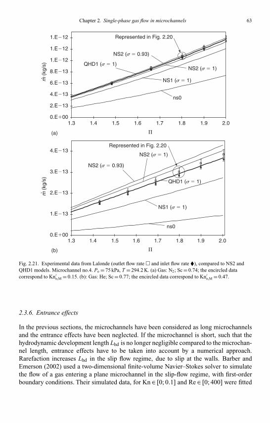
Kandlikar I044527-Ch02.tex 26/10/2005 18: 8 Page 63
Chapter 2. Single-phase gas flow in microchannels 63
0.E�00
2.E�13
4.E�13
6.E�13
8.E�13
1.E�12
1.E�12
1.E�12
1.3 1.4 1.5 1.6 1.7 1.8 1.9 2.0
Represented in Fig. 2.20
Represented in Fig. 2.20
(a)
0.E�00
1.E�13
2.E�13
3.E�13
4.E�13
1.3 1.4 1.5 1.6 1.7 1.8 1.9 2.0
(b)
NS2 (s � 0.93)
NS2 (s � 0.93)
ns0
ns0
NS2 (s � 1)
NS2 (s � 1)
NS1 (s � 1)
NS1 (s � 1)
QHD1 (s � 1)
QHD1 (s � 1)
m (
kg/s
)m
(kg
/s)
�
�
Fig. 2.21. Experimental data from Lalonde (outlet flow rate � and inlet flow rate �), compared to NS2 andQHD1 models. Microchannel no.4. Po = 75 kPa, T = 294.2 K. (a) Gas: N2; Sc = 0.74; the encircled datacorrespond to Kn′
o,M = 0.15. (b): Gas: He; Sc = 0.77; the encircled data correspond to Kn′o,M = 0.47.
2.3.6. Entrance effects
In the previous sections, the microchannels have been considered as long microchannelsand the entrance effects have been neglected. If the microchannel is short, such that thehydrodynamic development length Lhd is no longer negligible compared to the microchan-nel length, entrance effects have to be taken into account by a numerical approach.Rarefaction increases Lhd in the slip flow regime, due to slip at the walls. Barber andEmerson (2002) used a two-dimensional finite-volume Navier–Stokes solver to simulatethe flow of a gas entering a plane microchannel in the slip-flow regime, with first-orderboundary conditions. Their simulated data, for Kn ∈ [0; 0.1] and Re ∈ [0; 400] were fitted

Kandlikar I044527-Ch02.tex 26/10/2005 18: 8 Page 64
64 Heat transfer and fluid flow in minichannels and microchannels
Straight microchannel
Metal inter-connectsInlet/outlet Inlet/outlet
Integral pressure sensor
Metalinterconnects
Nitridemembrane
Piezoresistiveelements
Pressure sensor
Etching hole
Capillary connectionMicrochannel
(a)
(b)
Fig. 2.22. Microchannel with integrated pressure sensors (Zohar et al., 2002). (a) Microchannel with inlet andoutlet; (b) close-up of the pressure sensor and its capillary connection with the microchannel.
by a least-squares technique and led to the following expression for the hydrodynamicdevelopment length:
Lhd
DH= 0.332
0.0271 Re + 1+ 0.011 Re
1 + 14.78 Kn
1 + 9.78 Kn(2.160)
which generalizes the expression Lhd/DH = 0.315/(0.0175 Re + 1) + 0.011Re found byChen (1973) for a no-slip flow with a slight modification of the non-rarefied part of theequation. In Eq. (2.160), the Knudsen number Kn = λ/DH and the Reynolds numberRe = ρuzDH/µ are based on the hydraulic diameter DH = 4h of the microchannel, 2h indepth. The hydrodynamic development length is arbitrarily defined as the longitudinaldistance required for the centerline velocity to reach 99% of its fully developed value.Equation (2.160) shows that for Kn = 0.1 and Re = 400, slip at the wall increases theentrance length of about 25%.

Kandlikar I044527-Ch02.tex 26/10/2005 18: 8 Page 65
Chapter 2. Single-phase gas flow in microchannels 65
0
0.1
0.2
0.3
0.4
0.5
0.6
0.7
0.8
0.9
1
0 20,000 40,000 60,000 80,000 100,000f (Hz)
1
2
3
3�
2�
1�p∗
1
1�
2
3
2h � 4.14 µm
2h � 2.07 µm
2h � 1.03 µm
Fig. 2.23. Influence of microchannel depth 2h on the gain p∗ for a square microchannel closed at its outlet.l = 100 µm, T = 293 K, p = 0.11 MPa. 1, 2, 3: slip flow; 1′, 2′, 3′: no-slip flow.
2.4. Pulsed gas flows in microchannels
Rarefaction affects steady microflows and modifies the behavior of unsteady microflows.The case of pulsed flows is of particular interest because such flows are encounteredin many applications. For example, micropump actuators often generate sinusoidal pres-sure fluctuations inside a chamber in order to induce a flow in microchannels throughmicrovalves or microdiodes.
Detailed models for pulsed gaseous flows in the slip flow regime can be found in Caenet al. (1996) for circular microtubes or in Colin et al. (1998a) for rectangular microchannels.They are based on the Navier–Stokes equations with first-order slip and temperature jumpconditions at the walls. If we consider a microchannel of length l, whose inlet is submitted toa sinusoidal pressure fluctuation with a small amplitude, the gainp∗ of the microchannel,that is the ratio of the outlet po over inlet pi fluctuating pressures amplitudes, can becalculated. For example, in the simple case of a microchannel closed at its outlet, this gaintakes the form
p∗ =∣∣∣∣po
pi
∣∣∣∣ =∣∣∣∣ 1
cosh(βl)
∣∣∣∣ (2.161)
where β( f , Kn) ≈√f �(Kn) depends on the square root of the frequency f and on theKnudsen number. It can be shown that the band pass of the microchannel is underestimatedwhen slip at the walls is not taken into account (Fig. 2.23).
Obtaining experimental data to discuss these theoretical results is very hard, due tothe very small size of the pressure sensors required for these experiments. However,

Kandlikar I044527-Ch02.tex 26/10/2005 18: 8 Page 66
66 Heat transfer and fluid flow in minichannels and microchannels
i o
2b2 2b32b1
2b1 2b2 2b3
l1 l2 l3
i o
(a)
(b)
Fig. 2.24. Two layouts of a microdiode placed in a microchannel.
experimental data were obtained for microtubes down to 50 µm in diameter, using a com-mercially available pressure microsensor placed in a minichannel connected in series toone or several parallel microtubes (Colin et al., 1998b). The behavior of the micro- andminichannels association was simulated and compared to these data. The agreement wasgood, both for the gain and the phase of the association.
The model for pulsed flows in constant-section microchannels can be easily extendedto microchannels with slowly varying cross-sections (Aubert et al., 1998). It allows anunderstanding of the behavior of microdiffusers subjected to sinusoidal pressure fluctua-tions and to test the diode effect of a microdiffuser/nozzle placed in a microchannel thatis subjected to sinusoidal pressure fluctuations. In Fig. 2.24, two layouts (a) and (b) areconsidered.
In layout (a), the tested element is a microdiffuser, with an increasing section from inletto outlet. In layout (b), the same element is used as a nozzle with a decreasing section frominlet to outlet. To obtain an exploitable comparison between the two layouts, the widths(2b1, 2b2, 2b3) and the lengths (l1, l2, l3) are the same in layouts (a) and (b). The angle 2αis also the same for the diffuser or the nozzle.
An analysis of the frequency behavior for each layout shows significant differences,which is characteristic of a dynamic diode effect. Therefore, in order to characterize thedissymmetry of the transmission of the pressure fluctuations, an efficiency E of the diodeis introduced. This efficiency
E = p∗(a)
p∗(b)
= |po/pi|(a)
|po/pi|(b)(2.162)
defined as the ratio of the fluctuating pressure gain in layout (a) over the fluctuating pres-sure gain in layout (b), can be studied as a function of the frequency f . Some resultsare shown in Fig. 2.25, for different values of the depth 2 h with l1 = l2 = l3 = 3 mm,2b1 = 2b3 = 467 µm, 2b2 = 100 µm and α= 3.5◦.

Kandlikar I044527-Ch02.tex 26/10/2005 18: 8 Page 67
Chapter 2. Single-phase gas flow in microchannels 67
0.7
0.75
0.8
0.85
0.9
0.95
1
1.05
0 5000 10000 15000
E
f (Hz)
1 3
2
Fig. 2.25. Diode efficiency for different values of the depth. 1: 2h = 100 µm; 2: 2h = 62 µm, 3:2h = 6 µm.
Figure 2.25 points out that with a microdiffuser (2h = 6 µm), E appears to be less thanunity below a critical frequency. This denotes a reversed diode effect compared to the caseof a diffuser with sub-millimetric dimensions (2h = 100 µm), for which E is less than unitybeyond a critical frequency. Note also that the influence of slip (taken into account in Fig.2.25) is not negligible when 2h = 6 µm. However, slip has little influence on the valuesof characteristic frequencies (i.e. the frequencies for which E is an extremum or equal tounity).
Pulsed gaseous flows are also of great interest in short microchannels, or micro-orifices,for example in synthetic microjets. The synthetic microjet is a low power, highly compactmicrofluidic device that has potential for application in boundary layer control (Lee et al.,2003). The oscillation of an actuated membrane at the bottom of a cavity generates apulsed flow through a micro-slit or orifice (Fig. 2.26). It results in a zero net-mass flux,but in a non-zero mean momentum flux. A series of such microjets can be used to controlseparation or transition in the boundary layer of the flow on a wing in order to reduce drag,to increase lift or to limit noise generated by the air flow.
2.5. Thermally driven gas microflows and vacuum generation
Generating vacuum by means of microsystems concerns various applications such asthe taking of biological or chemical samples, or the control of the vacuum level in theneighborhood of some specific microsystems during working.
The properties of rarefied flows (due to both low pressure and small dimensions) allowunusual pumping techniques. For high Knudsen numbers, the flow may be generatedwithout any moving mechanical component by only using thermal actuation, which is notpossible with classical macropumps.
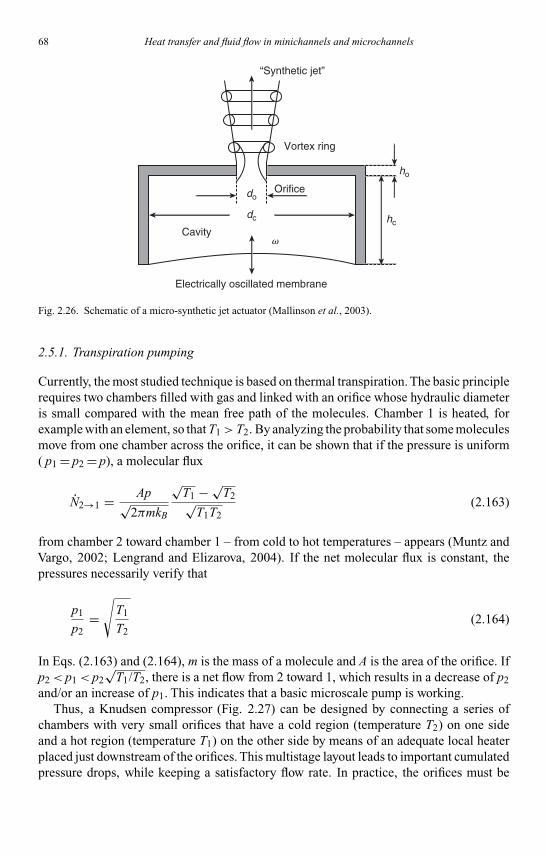
Kandlikar I044527-Ch02.tex 26/10/2005 18: 8 Page 68
68 Heat transfer and fluid flow in minichannels and microchannels
Electrically oscillated membrane
Cavity
Vortex ring
“Synthetic jet”
Orifice
v
dc
do
ho
hc
Fig. 2.26. Schematic of a micro-synthetic jet actuator (Mallinson et al., 2003).
2.5.1. Transpiration pumping
Currently, the most studied technique is based on thermal transpiration. The basic principlerequires two chambers filled with gas and linked with an orifice whose hydraulic diameteris small compared with the mean free path of the molecules. Chamber 1 is heated, forexample with an element, so that T1 >T2. By analyzing the probability that some moleculesmove from one chamber across the orifice, it can be shown that if the pressure is uniform( p1 = p2 = p), a molecular flux
N2→1 = Ap√2πmkB
√T1 − √
T2√T1T2
(2.163)
from chamber 2 toward chamber 1 – from cold to hot temperatures – appears (Muntz andVargo, 2002; Lengrand and Elizarova, 2004). If the net molecular flux is constant, thepressures necessarily verify that
p1
p2=√
T1
T2(2.164)
In Eqs. (2.163) and (2.164), m is the mass of a molecule and A is the area of the orifice. Ifp2 < p1 < p2
√T1/T2, there is a net flow from 2 toward 1, which results in a decrease of p2
and/or an increase of p1. This indicates that a basic microscale pump is working.Thus, a Knudsen compressor (Fig. 2.27) can be designed by connecting a series of
chambers with very small orifices that have a cold region (temperature T2) on one sideand a hot region (temperature T1) on the other side by means of an adequate local heaterplaced just downstream of the orifices. This multistage layout leads to important cumulatedpressure drops, while keeping a satisfactory flow rate. In practice, the orifices must be
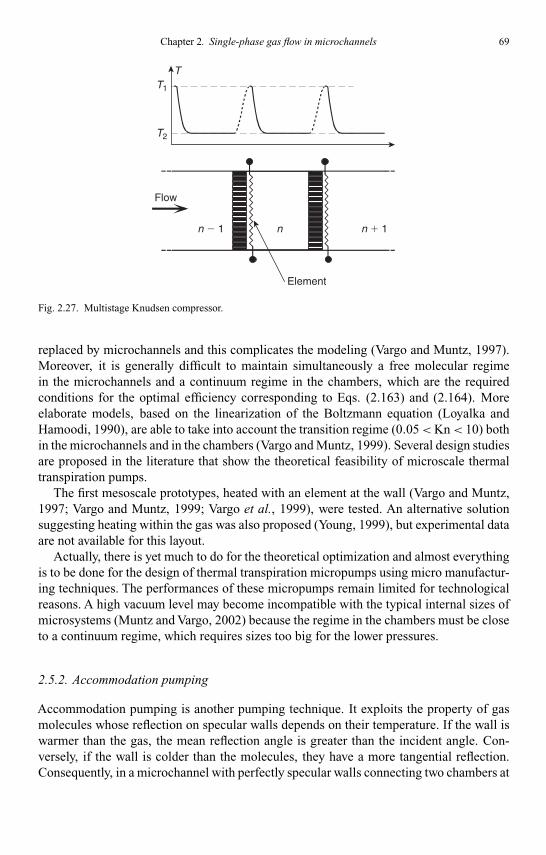
Kandlikar I044527-Ch02.tex 26/10/2005 18: 8 Page 69
Chapter 2. Single-phase gas flow in microchannels 69
n � 1 n � 1n
TT1
T2
Flow
Element
Fig. 2.27. Multistage Knudsen compressor.
replaced by microchannels and this complicates the modeling (Vargo and Muntz, 1997).Moreover, it is generally difficult to maintain simultaneously a free molecular regimein the microchannels and a continuum regime in the chambers, which are the requiredconditions for the optimal efficiency corresponding to Eqs. (2.163) and (2.164). Moreelaborate models, based on the linearization of the Boltzmann equation (Loyalka andHamoodi, 1990), are able to take into account the transition regime (0.05<Kn< 10) bothin the microchannels and in the chambers (Vargo and Muntz, 1999). Several design studiesare proposed in the literature that show the theoretical feasibility of microscale thermaltranspiration pumps.
The first mesoscale prototypes, heated with an element at the wall (Vargo and Muntz,1997; Vargo and Muntz, 1999; Vargo et al., 1999), were tested. An alternative solutionsuggesting heating within the gas was also proposed (Young, 1999), but experimental dataare not available for this layout.
Actually, there is yet much to do for the theoretical optimization and almost everythingis to be done for the design of thermal transpiration micropumps using micro manufactur-ing techniques. The performances of these micropumps remain limited for technologicalreasons. A high vacuum level may become incompatible with the typical internal sizes ofmicrosystems (Muntz and Vargo, 2002) because the regime in the chambers must be closeto a continuum regime, which requires sizes too big for the lower pressures.
2.5.2. Accommodation pumping
Accommodation pumping is another pumping technique. It exploits the property of gasmolecules whose reflection on specular walls depends on their temperature. If the wall iswarmer than the gas, the mean reflection angle is greater than the incident angle. Con-versely, if the wall is colder than the molecules, they have a more tangential reflection.Consequently, in a microchannel with perfectly specular walls connecting two chambers at

Kandlikar I044527-Ch02.tex 26/10/2005 18: 8 Page 70
70 Heat transfer and fluid flow in minichannels and microchannels
T3 � T1 T1
T2
1
2
3
Fig. 2.28. One stage of an accommodation micropump.
different temperatures, a flow takes place from the hot toward the cold chambers (Hobson,1970). If the walls of the microchannel give a diffuse reflection, this effect disappears.This property was confirmed with numerical simulations by the DSMC method (Hudsonand Bartel, 1999). By linking two warm chambers (1 and 3) to a cold chamber (2) on oneside with a smooth microchannel (1–2) and on the other side with a rough microchannel(3–2), a difference of pressure ( p1 < p3) appears between the two chambers at the sametemperature (Fig. 2.28).
Connecting in series several stages of that type, the pressure drops relative to eachstage can be cumulated and allow the setup to reach high vacuum levels. The advantage ofthe accommodation pump is that it is operational without theoretical limitations concern-ing low pressures and contrary to the thermal transpiration pumping, the accommodationpumping does not require chambers with high dimensions. To compensate, the accom-modation pump requires more stages to reach the same final pressure ratio. A pressureratio �= 100 requires 125 stages, whereas only 10 stages are enough for a transpirationpump with comparable temperatures. Lastly, no operational prototype was described in theliterature so far, although the concept seems attractive. The highest-performance designwas proposed by Hobson (1971; 1972); it requires a cold temperature T2 = 77 K for anatmospheric temperature T1 = T3 = 290 K.
2.6. Heat transfer in microchannels
In the slip flow regime, heat transfer can be treated as well as mass transfer, providing theenergy equation (2.41) and the temperature boundary conditions (2.61) are solved with themomentum equation and the slip-flow boundary conditions. Such heat transfer problemshave an analytical solution only in the simplest cases. For example, if the compressibilityof the flow can be neglected, the energy and the momentum equations are no longer
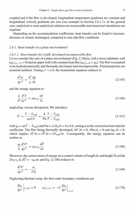
Kandlikar I044527-Ch02.tex 26/10/2005 18: 8 Page 71
Chapter 2. Single-phase gas flow in microchannels 71
coupled and if the flow is developed, longitudinal temperature gradients are constant andlongitudinal velocity gradients are zero (see example in Section 2.6.1.1). In the generalcase, analytical or semi-analytical solutions are not possible and numerical simulations arerequired.
Depending on the accommodation coefficients, heat transfer can be found to increase,decrease or remain unchanged, compared to non-slip-flow conditions.
2.6.1. Heat transfer in a plane microchannel
2.6.1.1. Heat transfer for a fully developed incompressible flowLet us consider the case of a plane microchannel (Fig. 2.10(a)), with a lower adiabatic wall(qw|y=−h = 0) and an upper wall with constant heat flux (qw|y=h = qh). The flow is assumedto be hydrodynamically and thermally developed and incompressible. Fluid properties areassumed uniform. Noting y∗ = y/h, the momentum equation reduces to
d2uz
dy∗2 = h2
µ
dp
dz(2.165)
and the energy equation to
k
h2
∂2T
∂y∗2 = ρuzcp∂T
∂z(2.166)
neglecting viscous dissipation. We introduce
θ∗ = T − Twall
qhh/k= 4
Nu
T − Twall
T − Twall(2.167)
with qh =α(T − Twall) and Nu =αDH/k = 4α h/k , noting α as the convection heat transfercoefficient. The flow being thermally developed, ∂θ∗/∂z = 0, ∂Nu/∂z = 0 and ∂qh/∂z = 0,which implies ∂T /∂z = ∂T /∂z = ∂Twall/∂z. Consequently, the energy equation can bewritten as
qh
h
d2θ∗
dy∗2 = ρuzcpdT
dz(2.168)
Moreover, the conservation of energy on a control volume of length dz and height 2h yields2h ρ cp uz dT = −qh dz and Eq. (2.168) reduces to
d2θ∗
dy∗2 = − uz
2 uz(2.169)
Neglecting thermal creep, the first-order boundary conditions are
duz
dy∗
∣∣∣∣y∗=0 = 0 uz|y∗=1 = −ξ∗ duz
dy∗
∣∣∣∣y∗=1
(2.170)

Kandlikar I044527-Ch02.tex 26/10/2005 18: 8 Page 72
72 Heat transfer and fluid flow in minichannels and microchannels
dθ∗
dy∗
∣∣∣∣y∗=−1
= 0 θ∗|y∗=1 = −ς∗ dθ∗
dy∗
∣∣∣∣y∗=1
(2.171)
with a dimensionless coefficient of slip ξ∗ = ξ/h = (λ/h)(2 − σ)/σ= 4 Kn(2 − σ)/σ anda dimensionless temperature jump distance ς∗ = ς/h = (λ/h)[(2 − σT )/σT ][2γ/(γ + 1)]/Pr = 8 [(2 − σT )/σT ][γ/(γ + 1)][Kn/Pr], where Pr is the Prandtl number. The resolutionof this set of equations gives the velocity distribution
uz = − h2
2µ
dp
dz(1 − y∗2 + 2 ξ∗) (2.172)
and, with
uz = 1
2
∫ 1
−1uz dy∗
uz
uz= 3(−y∗2 + 1 + 2 ξ∗)
2(1 + 3 ξ∗)(2.173)
The integration of Eq. (2.169) with the boundary conditions (2.171) yields
θ∗ = ς∗ + 1
1 + 3 ξ∗
[1
16y∗4 − 3
8y∗2(1 + 2 ξ∗) − 1
2y∗(1 + 3 ξ∗)
+(
13
16+ 9
4ξ∗)]
(2.174)
T and T = (1/2)∫ 1−1 (uz/uz)T dy∗ are calculated and the Nusselt number is deduced as
Nu−1 = ς∗
4+ 26 + 147 ξ∗ + 210 ξ∗2
140 (1 + 3 ξ∗)2(2.175)
Equation (2.175) shows that heat transfer depends both on the dimensionless coefficientof slip ξ∗ and on the dimensionless temperature jump distance ς∗, that is it depends onthe two accommodation coefficients σ and σT as well as on the Knudsen number Kn. Forclassical values of the accommodation coefficients, the effect of the temperature jump isgreater than the effect of velocity slip and the heat transfer decreases when rarefactionincreases. The Nusselt number reduces to the classic value 70/13 (Rohsenow, 1998) whenKn = 0.
Zhu et al. (2000) extended this solution to the problem of asymmetrically heated walls(0 �= q0 �= qh) by combining the solutions of two sub-problems similar to the above problem.
Inman (Karniadakis and Beskok, 2002) first studied the solution for a constantsymmetric heat flux at the two walls.

Kandlikar I044527-Ch02.tex 26/10/2005 18: 8 Page 73
Chapter 2. Single-phase gas flow in microchannels 73
The problem with constant wall temperature was treated by Hadjiconstantinou andSimek (2002), who extended the study to the transition regime, using DSMC. They showedthat the slip flow prediction (with first-order boundary conditions) is in good agreementwith the DSMC results for Kn ≤ 0.2 and remains a good approximation beyond its expectedrange of applicability.
2.6.1.2. Heat transfer for a developing compressible flowThis problem was studied by Kavehpour et al. (1997), using the same first-order slip flowand temperature jump boundary conditions as in Section 2.6.1.1. The flow was developingboth hydrodynamically and thermally and two cases were considered: uniform wall tem-perature or uniform wall heat flux. Viscous dissipation was neglected, but compressibilitywas taken into account. The numerical methodology was based on the control volumefinite difference scheme. It was found that the Nusselt number was substantially reducedfor slip flow compared with continuum flow.
2.6.2. Heat transfer in a circular microtube
Heat transfer in circular microtubes was simulated by Ameel et al. (1997), who consid-ered a hydrodynamically fully developed incompressible flow, thermally developing withconstant heat flux at the wall. Viscous dissipation and thermal creep were neglected andfirst-order velocity slip and temperature jump conditions were used, with accommodationcoefficients taken equal to unity.
They found the thermally fully developed solution
Nu−1 = 24χ2 − 16χ+ 3
48(2χ− 1)2
(1 + 24γ(χ− 1)(2χ− 1)2
(24χ2 − 16χ+ 3)(γ + 1) Pr
)(2.176)
with χ= 1 + 4 Kn. Equation (2.176) reduces to the no-slip value Nu = 48/11 when Kn = 0.A semi-analytical solution is also given in Ameel et al. (1997) for the entrance region. Fora Knudsen number Kn = 0.04, it is found that the Nusselt number for the fully developedflow is reduced 14% over that obtained with a no-slip boundary condition, with γ = 1.4and Pr = 0.7.
Larrodé et al. (2000) treated the case of constant temperature at the wall.
2.6.3. Heat transfer in a rectangular microchannel
Yu and Ameel (2001) studied the heat transfer problem for a thermally developing flowin a rectangular microchannel. The flow was assumed to be incompressible and hydro-dynamically fully developed, and a constant temperature was imposed at the walls. Thevelocity distribution was developed in series as discussed in Section 2.3.4.1 and the energyequation was solved by a modified generalized integral transform method. A competitionbetween ξ and ς was pointed out, with a transition value βc of β= ξ/ς that depends on theaspect ratio a∗ (Table 2.7).

Kandlikar I044527-Ch02.tex 26/10/2005 18: 8 Page 74
74 Heat transfer and fluid flow in minichannels and microchannels
Table 2.7Transition values of β= ξ/ς as a function of the aspect ratio, (from Yu and Ameel(2001)).
a∗−1 1 2 3 4 5 6 8 10 ∞
βc 0.67 0.50 0.38 0.32 0.29 0.28 0.27 0.25 0.20
For β<βc, heat transfer is enhanced in comparison with the no-slip flow and if β>βc,heat transfer is reduced. Moreover, for β<βc, heat transfer increases with increasing ξ∗and it decreases if β<βc. According to the values available in the literature, it should benoted that β may vary in a wide range from unity to 100 or more, for actual wall surfaceconditions. However, the value β= 1.67, which corresponds to a diffuse reflection (σ= 1)and a total thermal accommodation (σT = 1) for air (γ = 1.4; Pr = 0.7) is a representativevalue for many engineering applications. In this typical case, rarefaction effects result ina decrease of heat transfer, which can be as much as 40%.
2.7. Future research needs
Theoretical knowledge is currently well advanced for gas flows in microchannels. How-ever, there is yet a need for accurate experimental data, both for steady or unsteady gasmicroflows, with or without heat transfer. For example, in order to definitely validate thechoice of the best boundary conditions in the slip flow regime, we need to isolate the influ-ence of the accommodation coefficients, as it remains an open issue. Relationships betweentheir values, the nature of the substrate and the micro-fabrication processes involved arecurrently not available. Theoretical investigations relative to unsteady or thermally drivenmicroflows would also need to be supported by smart experiments.
2.8. Solved examples
Example 2.1
A microchannel with constant rectangular cross-section is submitted to a pressure-drivenflow of argon. The inlet and the outlet pressures are pi = 0.2 MPa and po = 25 kParespectively. The geometry is given in Fig. 2.10(c), with a width 2b = 20 µm, a depth2h = 1 µm and a length l = 5 mm.
Assume a uniform temperature T = 350 K.
(i) Calculate the Knudsen numbers Kn and Kn′ at the inlet and at the outlet of themicrochannel, assuming that the intermolecular collisions are accurately describedby a variable soft spheres model.
(ii) Compare with the values obtained from a hard spheres model.(iii) Assuming a diffuse reflection at the wall, calculate the mass flow rate through the
microchannel.

Kandlikar I044527-Ch02.tex 26/10/2005 18: 8 Page 75
Chapter 2. Single-phase gas flow in microchannels 75
(iv) Calculate the mass flow rate increase (in %) due to slip at the wall.(v) What would be the underestimation (in %) of the mass flow rate given by a no-slip
model, in the same conditions but with an inlet pressure pi = 0.1 MPa?
Solution:(i) Inlet and outlet Knudsen numbers with aVSS model (Answer: Kn′
i = 3.48 × 10⁻²;Kni = 1.83 × 10⁻²; Kn′
o = 2.78 × 10⁻¹; Kno = 1.46 × 10⁻¹)From Table 2.2, the temperature exponent of the coefficient of viscosity for argon (Ar) isω= 0.81, the exponent for the VSS model is α= 1.40 and the dynamic viscosity understandard conditions is µ0 = 211.7 × 10⁻⁷ Pa s.
From Eq. (2.7), the viscosity at T = 350 K is:
µ(T ) = µ0(T /T0)ω = 2.117 × 10⁻⁵(350/273.15)0.81 = 2.588 × 10⁻⁵ Pa s.
The molecular weight of argon is given in Table 2.2: M = 39.948 × 10⁻³ kg/mol and itsgas constant is R = R/M = 8.314511/39.948 × 10−3 = 2.08 × 10² J/kg/K.
The mean free path is given by Table 2.1: λ= k2µ(T )√
RT /p,with
k2,VSS = 4α(7 − 2ω)(5 − 2ω)
5(α+ 1)(α+ 2)√
2π= 0.996.
At the inlet,
λi,VSS = k2µ(T )√
RT /pi = 0.996 × 2.588 × 10−5 ×√
2.08 × 102 × 350/2 × 105
= 34.8 nm
and at the outlet,
λo,VSS = k2µ(T )√
RT /po = 0.996 × 2.588 × 10−5 ×√
2.08 × 102 × 350/2.5 × 104
= 278 nm.
The Knudsen number based on the hydraulic diameter
DH = 4bh/(b + h) = 4 × 10 × 10−6 × 0.5 × 10−6/((10 + 0.5) × 10−6) = 1.905 µm
is Kn = λ/DH, that is
Kni = λi/DH = 3.48 × 10⁻⁸/1.905 × 10−6 = 1.83 × 10⁻² at the inlet and
Kno = λo/DH = 2.78 × 10⁻⁷/1.905 × 10−6 = 1.46 × 10⁻¹at the outlet.
The Knudsen number based on the microchannel depth is Kn′ = λ/(2h), that is
Kn′i = λi/(2 h) = 3.48 × 10⁻⁸/1 × 10−6 = 3.48 × 10⁻² at the inlet and

Kandlikar I044527-Ch02.tex 26/10/2005 18: 8 Page 76
76 Heat transfer and fluid flow in minichannels and microchannels
Kn′o = λo/(2h) = 2.78 × 10⁻⁷/1 × 10−6 = 2.78 × 10⁻¹at the outlet.
(ii) Inlet and outlet Knudsen numbers with a HS model (Answer: Kn′i,HS = 4.13 × 10⁻²;
Kni,HS = 2.17 × 10⁻²; Kn′o,HS = 3.30 × 10⁻¹; Kno,HS = 1.73 × 10⁻¹)
With a HS model, ω= 0.5 and the viscosity
µ(T ) = µ0(T/T0)0.5 = 2.117 × 10⁻⁵(350/273.15)0.5
= 2.396 × 10⁻⁵ Pa s is underestimated of 7.4%.
The coefficient k2,HS = 16/(5√
2π) = 1.277 (cf. Table 2.1).Consequently,
λi,HS = k2,HS µ(T )√
RT /pi = 1.277 × 2.588 × 10−5 ×√
2.08 × 102 × 350/2 × 105
= 41.3 nm
and
λo,HS = k2,HS µ(T )√
RT /po = 1.277 × 2.588 × 10−5 ×√
2.08 × 102 × 350/2.5 × 104
= 330 nm
which leads to:
Kni,HS = λi,HS/DH = 4.13 × 10⁻⁸/1.905 × 10−6 = 2.17 × 10⁻²
Kno,HS = λo,HS/DH = 3.30 × 10⁻⁷/1.905 × 10−6 = 1.73 × 10⁻¹
Kn′i,HS = λi,HS/(2 h) = 4.13 × 10⁻⁸/1 × 10−6 = 4.13 × 10⁻²
Kn′o,HS = λo,HS/(2 h) = 3.30 × 10⁻⁷/1 × 10−6 = 3.30 × 10⁻¹
The overestimation of the Knudsen number calculated from an HS model, comparedwith the more accurate solution obtained with a VSS model, is 28.2%, which correspondsto the ratio (k2,HS − k2,VSS)/k2,VSS = 0.282.
(iii) Mass flow rate (Answer: m = 4.89 × 10⁻¹² kg/s)The rectangular cross-section has a non-negligible aspect ratio a∗ = h/b = 1/20 = 0.05>0.01. Therefore, a rectangular model should be used. Due to the range covered by theKnudsen numbers, a second-order model (NS2) is required (cf. Fig. 2.7).
The mass flow rate is obtained from Eq. (2.157):
mNS2, rect = 4 h4p2o
a∗µRTl
[a1
2(�2 − 1) + a2 Kn′
o(�− 1) + a3Kn′2o ln�
]

Kandlikar I044527-Ch02.tex 26/10/2005 18: 8 Page 77
Chapter 2. Single-phase gas flow in microchannels 77
with a1 = 0.32283, a2 = 1.9925 and a3 = 4.2853 given by Table 2.5 for a diffuse reflection(σ= 1). �= pi/po = 200/25 = 8 and
mNS2, rect = 4(10−6)4(2.5 × 10⁻⁴)2/(0.05 × 2.588 × 10−5 × 2.08 × 102 × 350
× 5 × 10−3)× [0.32283(82 − 1)/2 + 1.9925 × 2.78 × 10−1(8 − 1)
+ 4.2853 × (2.78 × 10−1)2ln8] = 4.89 × 10⁻¹² kg/s
(iv) Mass flow rate increase (Answer: 44.9%)From Eq. (2.158),
m∗NS2, rect = mNS2, rect
mns, rect=[
1 + 2a2
a1Kn′
o1
�+ 1+ 2
a3
a1Kn′2
oln�
�2 − 1
]
= 1 + 21.9925
0.322832.78 × 10−1 1
8 + 1+ 2
4.2853
0.32283(2.78×10⁻¹)2 ln 8
82 − 1= 1.449
which means that slip at the wall increases the flow rate of 44.9%.
(v) Underestimation of the mass flow rate (Answer: 46.7%)If the inlet pressure is decreased to pi = 0.1 MPa, the pressure ratio is �= 4 and
m∗NS2, rect = 1+2
1.9925
0.322832.78×10−1 1
4 + 1+ 2
4.2853
0.32283(2.78 × 10⁻¹)2 ln 4
42 − 1= 1.877.
Therefore, although the outlet Knudsen number is unchanged, the inlet pressure numberis increased and rarefaction effects are enhanced. Slip at the wall now increases the flowrate of 87.7%. In others words, the underestimation of the mass flow rate with a no-slipmodel is 46.7%, since (mNS2 − mns)/mNS2 = 1 − 1/m∗
NS2 = 1 − 1/1.877 = 0.467.
Example 2.2
In a hard disk drive, the flow of gas between the hard disk and the read–write head canlocally be comparable to a fully developed micro-Couette flow between parallel planeplates. The shield of the hard disk drive is sealed and the gas inside is pure nitrogen. Thedistance between the two plates is 2h = 0.2 µm, the read-write head is at r = 3 cm from thecenter of the disk, whose speed of rotation is ω= 7200 rpm. One of the plates (y = −h) isfixed and the other (y = h) moves with a constant velocity U in the z-direction.
Assume a uniform temperature T = 300 K, a uniform pressure p = 90 kPa and anaccommodation coefficient σ= 0.9.
(i) Write the velocity distribution as a function of the Knudsen number.(ii) Calculate the mass flow rate per unit width and compare it to the case of a no-slip
Couette flow.(iii) Calculate the friction factor and compare its value to the one obtained with a no-slip
assumption.
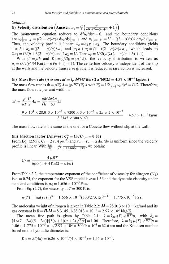
Kandlikar I044527-Ch02.tex 26/10/2005 18: 8 Page 78
78 Heat transfer and fluid flow in minichannels and microchannels
Solution(i) Velocity distribution
(Answer: uz = U
2
(y∗
4 Kn(2−σ)/σ + 1 + 1))
The momentum equation reduces to d2uz/dy2 = 0, and the boundary conditionsare uz
∣∣y=−h = ((2 − σ)/σ)λ duz/dy∣∣y=−h and uz
∣∣y=+h = U − ((2 − σ)/σ)λ duz/dy∣∣y=+h.
Thus, the velocity profile is linear: uz = a1 y + a2. The boundary conditions yields−a1 h + a2 = ((2 − σ)/σ)λ a1 and a1 h + a2 = U − ((2 − σ)/σ)λ a1, which leads to2 a1 = U /(h + λ(2 − σ)/σ) and 2 a2 = U . Then uz = U /2(y/(λ(2 − σ)/σ+ h) + 1).
With y∗ = y/h and Kn = y/DH = y/(4 h), the velocity distribution is written asuz = U /2(y∗/(4 Kn(2 − σ)/σ+ 1) + 1). The centerline velocity is independent of the slipat the walls and the velocity transverse gradient is reduced as rarefaction is increased.
(ii) Mass flow rate (Answer: m′ = (p M/RT )(ω r 2 π/60)2h = 4.57 × 10⁻⁶ kg/s/m)The mass flow rate is m = ρ uz A = (p/RT ) uz A with uz = 1/2
∫ 1−1 uz dy∗ = U /2. Therefore,
the mass flow rate per unit width is:
m′ = p
RT
U
24h = pM
RT
ωr2π
602h
= 9 × 104 × 28.013 × 10−3 × 7200 × 3 × 10−2 × 2π × 2 × 10−7
8.3145 × 300 × 60= 4.57 × 10⁻⁶ kg/m
The mass flow rate is the same as the one for a Couette flow without slip at the wall.
(iii) Friction factor (Answer: C∗f = Cf/Cf ,ns = 0.57)
From Eq. (2.95), Cf = 2 τw/(ρuz2) and τw = τw =µ duz/dy is uniform since the velocity
profile is linear. With duzdy = U
2 h1
1 + 4 Kn(2 − σ)/σ , we obtain:
Cf = 4µRT
hpU (1 + 4 Kn(2 − σ)/σ)
From Table 2.2, the temperature exponent of the coefficient of viscosity for nitrogen (N2)is ω= 0.74, the exponent for the VSS model is α= 1.36 and the dynamic viscosity understandard conditions is µ0 = 1.656 × 10⁻⁵ Pa s.
From Eq. (2.7), the viscosity at T = 300 K is:
µ(T ) = µ0(T /T0)ω = 1.656 × 10⁻⁵(300/273.15)0.74 = 1.775×10⁻⁵ Pa s.
The molecular weight of nitrogen is given in Table 2.2: M = 28.013 × 10⁻³ kg/mol and itsgas constant is R = R/M = 8.314511/28.013 × 10−3 = 2.97 × 10² J/kg/K.
The mean free path is given by Table 2.1: λ= k2µ(T )√
RT /p, with k2 =[4α(7 − 2ω)(5 − 2ω)]/[5(α+ 1)(α+ 2)
√2π] = 1.06. Therefore, λ= k2 µ(T )
√RT /p =
1.06 × 1.775 × 10−5 × √2.97 × 102 × 300/9 × 104 = 62.6 nm and the Knudsen number
based on the hydraulic diameter is:
Kn = λ/(4h) = 6.26 × 10⁻⁸/(4 × 10−7) = 1.56 × 10⁻¹.
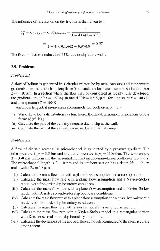
Kandlikar I044527-Ch02.tex 26/10/2005 18: 8 Page 79
Chapter 2. Single-phase gas flow in microchannels 79
The influence of rarefaction on the friction is then given by:
C∗f = Cf Cf ,ns = Cf /Cf (Kn=0) = 1
1 + 4Kn(2 − σ)/σ
= 1
1 + 4 × 0.156(2 − 0.9)/0.9= 0.57
The friction factor is reduced of 43%, due to slip at the walls.
2.9. Problems
Problem 2.1
A flow of helium is generated in a circular microtube by axial pressure and temperaturegradients. The microtube has a length l = 5 mm and a uniform cross-section with a diameter2 r2 = 10 µm. In a section where the flow may be considered as locally fully developed,the gradients are dp/dz = −5 Pa/µm and dT /dz = 0.5 K/µm, for a pressure p = 100 kPaand a temperature T = 400 K.
Assume a tangential momentum accommodation coefficient σ= 0.9.
(i) Write the velocity distribution as a function of the Knudsen number, in a dimensionlessform: u∗
z (r∗, Kn).(ii) Calculate the part of the velocity increase due to slip at the wall.
(iii) Calculate the part of the velocity increase due to thermal creep.
Problem 2.2
A flow of air in a rectangular microchannel is generated by a pressure gradient. Theinlet pressure is pi = 3.5 bar and the outlet pressure is po = 150 mbar. The temperatureT = 350 K is uniform and the tangential momentum accommodation coefficient is σ= 0.8.The microchannel length is l = 10 mm and its uniform section has a depth 2h = 1.2 µmand a width 2b = 4.8 µm.
(i) Calculate the mass flow rate with a plane flow assumption and a no-slip model.(ii) Calculate the mass flow rate with a plane flow assumption and a Navier–Stokes
model with first-order slip boundary conditions.(iii) Calculate the mass flow rate with a plane flow assumption and a Navier–Stokes
model with Deissler second-order slip boundary conditions.(iv) Calculate the mass flow rate with a plane flow assumption and a quasi-hydrodynamic
model with first-order slip boundary conditions.(v) Calculate the mass flow rate with a no-slip model in a rectangular section.
(vi) Calculate the mass flow rate with a Navier–Stokes model in a rectangular sectionwith Deissler second-order slip boundary conditions.
(vii) Calculate the deviations of the above different models, compared to the most accurateamong them.

Kandlikar I044527-Ch02.tex 26/10/2005 18: 8 Page 80
80 Heat transfer and fluid flow in minichannels and microchannels
Problem 2.3
Consider a microchannel with a uniform cross-section whose width is very large comparedwith its depth 2h = 5 µm. A pressure-driven flow of helium is generated, the lower wall(y = −h) is adiabatic and the upper wall (y = h) has a constant heat flux qh = −200 W/cm2.Consider a section far from the inlet, such that the flow in this section is thermally andhydrodynamically developed. The flow conditions in this section are such that the Knudsennumber based on the hydraulic diameter is Kn = 2 × 10⁻² and the accommodation coef-ficients are σ= 0.9 and σT = 0.6. The wall temperature Twall = 400 K is measured with amicro-sensor.
(i) Calculate the mean temperature T of the gas in the section.(ii) Calculate the temperature T0 at the center of the section (y = 0).
(iii) Compare with the case of a similar non rarefied flow.
Problem 2.4
Consider a microchannel, with a length l = 5 mm and whose uniform rectangular cross-section has a low aspect ratio: its width is 2b = 200 µm and its depth is 2h = 1.5 µm. Aflow of nitrogen is generated with a pressure gradient. The inlet pressure is pi = 3 × 10⁵ Paand the outlet pressure is po = 1 × 10⁵ Pa. The temperature T = 300 K is uniform and thetangential momentum accommodation coefficient is σ= 0.95.
(i) Calculate the mean velocity in a cross-section of the microchannel, as a function ofthe local pressure gradient and Knudsen number.
(ii) Calculate the mass flow rate.(iii) Calculate the pressure value at the middle of the microchannel (at z = l/2) and compare
it to the no-slip value.(iv) Calculate the maximal velocity reached in the microchannel outside the entrance
region.(v) Calculate the maximal Mach number and justify the locally fully developed
assumption.
Problem 2.5
A multistage Knudsen compressor is designed to locally tune the pressure level or airinside a microsystem. The geometry of this Knudsen compressor is given in Fig. 2.27.Ten chambers are connected via 9 series of 100 short microchannels. These microchannelshave rectangular cross-sections with a depth 2h = 0.5 µm and a width 2b = 20 µm. Eachchamber is assumed large enough for the flow inside to be considered as a continuumflow. The temperature in these chambers is T2 = 300 K and each element is able to risethe temperature at the outlet of the microchannels to the value T1 = 600 K. Chamber 10 isconnected to a region, whose pressure p10 = 10 mbar is maintained constant by means of aprimary pump. The initial temperature Tt=0 = T2 = 300 K is uniform before the elementsheating. The initial pressure in each chamber is also uniform and is equal to the pressure

Kandlikar I044527-Ch02.tex 26/10/2005 18: 8 Page 81
Chapter 2. Single-phase gas flow in microchannels 81
in chamber 10: pt=0 = p10 = 10 mbar. For t > 0, heating of the elements can be regulatedin order to tune the pressure in chamber 1 in the range 1 to 10 mbar.
(i) Calculate the possible range covered by the Knudsen number in the microchannelsduring the pumping process and check that the free molecular regime assumption inthe microchannel is valid.
(ii) Calculate the maximal value of the mass flow rate between two adjacent chambers atthe beginning of the pumping progress.
(iii) Give the different reasons why the real initial mass flow rate is lower than the valuecalculated in (ii).
(iv) Calculate the minimal pressure value that can be reached in chamber 1 at the end ofthe pumping process.
Problem 2.6
Consider a pressure-driven flow of different gases (He, O2 or SO2), through a microtubewith rough walls, such that the accommodation coefficient can reasonably be assumedequal to unity. The microtube length is l = 3 mm and its inner diameter is 2 r2 = 1.2 µm.The inlet pressure is pi = 2 bar and the outlet pressure is po = 1 bar.
Assume that the intermolecular collisions are accurately described by a VSS model.
(i) Calculate the mass flow rate through this microtube for the three different gases usinga QHD1 model.
(ii) Calculate the mass flow rate through this microtube for the different gases using aNS2 model with Deissler boundary conditions.
(iii) Calculate the mass flow rate through this microtube for the different gases using aNS2 model with Chapman and Cooling boundary conditions.
(iv) Calculate the mass flow rate through this microtube for the different gases using aNS2 model with Mitsuya boundary conditions.
(v) Compare and comment on these different results.(vi) Propose an experimental protocol in order to check the more appropriate among the
above models.
References
Agarwal, R. K., Yun, K.-Y., and Balakrishnan, R., Beyond Navier–Stokes: Burnett equations forflows in the continuum–transition regime, Phys. Fluids, 13(10), 3061–3085, 2001.
Ameel, T. A., Wang, X., Barron, R. F., and Warrington, R. O. J., Laminar forced convection ina circular tube with constant heat flux and slip flow, Microscale Therm. Eng., 1(4), 303–320,1997.
Anderson, J. D., Modern Compressible Flow, 2 edn., New York: Mac Graw-Hill InternationalEditions, 1990.
Anduze, M., Etude expérimentale et numérique de microécoulements liquides dans les microsys-tèmes fluidiques, PhD Thesis, Toulouse: Institut National des Sciences Appliquées de Toulouse,2000.

Kandlikar I044527-Ch02.tex 26/10/2005 18: 8 Page 82
82 Heat transfer and fluid flow in minichannels and microchannels
Arkilic, E. B., Breuer, K. S., and Schmidt, M. A., Gaseous flow in microchannels, in Application ofMicrofabrication to Fluid Mechanics, Vol. FED-197. New York: ASME, pp. 57–66, 1994.
Arkilic, E. B., Schmidt, M. A., and Breuer, K. S., Sub-nanomol per second flow measurement nearatmospheric pressure, Exp. Fluid, 25(1), 37–41, 1998.
Arkilic, E. B., Breuer, K. S., and Schmidt, M. A., Mass flow and tangential momentumaccommodation in silicon micromachined channels, J. Fluid Mech., 437, 29–43, 2001.
Aubert, C., Ecoulements compressibles de gaz dans les microcanaux: effets de raréfaction, effetsinstationnaires, PhD Thesis, Toulouse: Université Paul Sabatier, 1999.
Aubert, C. and Colin, S., High-order boundary conditions for gaseous flows in rectangularmicrochannels, Microscale Therm. Eng., 5(1), 41–54, 2001.
Aubert, C., Colin, S., and Caen, R., Unsteady gaseous flows in tapered microchannels, in FirstInternational Conference on Modeling and Simulation of Microsystems, Semiconductors, Sensorsand Actuators (MSM’98), Vol. 1. Santa Clara Marriot: Computational Publications, pp. 486–491,1998.
Barber, R. W. and Emerson, D. R., The influence of Knudsen number on the hydrodynamicdevelopment length within parallel plate micro-channels, in Advances in Fluid Mechanics IV,M. Rahman, R. Verhoeven, and C. A. Brebbia, Eds., Southampton: WIT Press, pp. 207–216,2002.
Beskok, A. and Karniadakis, G. E., A model for flows in channels, pipes, and ducts at micro andnano scales, Microscale Therm. Eng., 3(1), 43–77, 1999.
Bhatnagar, P., Gross, E., and Krook, K., A model for collision processes in gasses, Phys. Rev., 94,511–524, 1954.
Bird, G., Monte Carlo simulation of gas flows, Annu. Rev. Fluid Mech., 10, 11–31, 1978.Bird, G. A., Molecular Gas Dynamics and the Direct Simulation of Gas Flows. Oxford: Clarendon
Press, 1998.Caen, R., Mas, I., and Colin, S., Ecoulements non permanents dans les microcanaux: réponse
fréquentielle des microtubes pneumatiques, C. R. Acad. Sci., Sér. II b, 323(12), 805–812,1996.
Cercignani, C., Illner, R., and Pulvirenti, M., The Mathematical Theory of Dilute Gases, Vol. 106.New York: Springer-Verlag, 1994.
Chapman, S. and Cowling, T. G., The Mathematical Theory of Non-uniform Gases. Cambridge:University Press, 1952.
Chen, C. S., Lee, S. M., and Sheu, J. D., Numerical analysis of gas flow in microchannels, Numer.Heat Transf., A, 33, 749–762, 1998.
Chen, R.-Y., Flow in the entrance region at low Reynolds numbers, J. Fluid. Eng., 95, 153–158,1973.
Chen, S. and Doolen, G., Lattice Boltzmann method for fluid flows, Annu. Rev. Fluid Mech., 30,329–364, 1998.
Cheng, H. and Emmanuel, G., Perspectives on hypersonic nonequilibrium flow, AIAA Journal, 33,385–400 1995.
Colin, S., Microfluidique. Paris: Lavoisier – Hermès Science Publications, 2004.Colin, S., Aubert, C., and Caen, R., Unsteady gaseous flows in rectangular microchannels: frequency
response of one or two pneumatic lines connected in series, Eur. J. Mech. B, Fluid, 17(1), 79–104,1998a.
Colin, S., Anduze, M., and Caen, R., A pneumatic frequency generator for experimental analysisof unsteady microflows, in Micro-Electro-Mechanical Systems (MEMS) – 1998, Vol. DSC-66,F. K. F. Liwei Lin, Narayan. R. Aluru, Xiang Zhang, Eds., NewYork: ASME, pp. 231–239, 1998b.
Colin, S., Elizarova, T. G., Sheretov, Y. V., Lengrand, J.-C., and Camon, H., Micro-écoulementsgazeux: validation expérimentale de modèles QHD et de Navier–Stokes avec conditions aux
Kandlikar I044527-Ch02.tex 26/10/2005 18: 8 Page 83
Chapter 2. Single-phase gas flow in microchannels 83
limites de glissement, in 16ème Congrès Français de Mécanique, Proceedings on CDROM,Nice, 2003.
Colin, S., Lalonde, P., and Caen, R., Validation of a second-order slip flow model in rectangularmicrochannels, Heat Transfer Eng., 25(3), 23–30, 2004.
Comeaux, K. A., Chapman, D. R., and MacCormack, R. W., An analysis of the Burnett equationsbased in the second law of thermodynamics, AIAA Paper, no. 95-0415, 1995.
Deissler, R. G., An analysis of second-order slip flow and temperature-jump boundary conditionsfor rarefied gases, Int. J. Heat Mass Transfer, 7, 681–694, 1964.
Ebert, W. A. and Sparrow, E. M., Slip flow in rectangular and annular ducts, J. Basic Eng., 87,1018–1024, 1965.
Elizarova, T. G. and Sheretov, Y. V., Analyse du problème de l’écoulement gazeux dans lesmicrocanaux par les équations quasi hydrodynamiques, La Houille Blanche, 5, 66–72, 2003.
Gad-el-Hak, M., Stokes’ hypothesis for a newtonian, isotropic fluid, J. Fluids Eng., 117, 3–5, 1995.Gad-el-Hak, M., The fluid mechanics of microdevices – The Freeman Scholar Lecture, J. Fluids
Eng., Vol. 121, pp. 5–33, 1999.Grad, H., On the kinetic theory of rarefied gases, Comm. Pure Appl. Math., 2, 331–407, 1949.Guo, Z. Y. and Wu, X. B., Further study on compressibility effects on the gas flow and heat transfer
in a microtube, Microscale Therm. Eng., 2(2), 111–120, 1998.Hadjiconstantinou, N. G. and Simek, O., Constant-wall-temperature Nusselt number in micro and
nano-channels, J. Heat Transf., 124, 356–364, 2002.Harley, J. C., Huang, Y., Bau, H. H., and Zemel, J. N., Gas flow in micro-channels, J. Fluid Mech.,
284, 257–274, 1995.Hassan, H. A. and Hash, D. B., A generalized hard-sphere model for Monte Carlo simulation, Phys.
Fluids A, 5(3), 738–744, 1993.Hobson, J. P., Accommodation pumping – A new principle for low pressure, J. Vac. Sci. Technol.,
7(2), 301–357, 1970.Hobson, J. P., Analysis of accommodation pumps, J. Vac. Sci. Technol., 8(1), 290–293, 1971.Hobson, J. P., Physical factors influencing accommodation pumps, J. Vac. Sci. Technol., 9(1), 252–
256, 1972.Hsia, Y.-T. and Domoto, G. A., An experimental investigation of molecular rarefaction effects in gas
lubricated bearings at ultra-low clearances, J. Lubr. Technol., 105, 120–130, 1983.Hudson, M. L. and Bartel, T. J., DSMC simulation of thermal transpiration and accommodation
pumps, in Rarefied Gas Dynamics, Vol. 1, R. Brun, R. Campargue, R. Gatignol, and J.-C.Lengrand, Eds., Cépaduès Editions, Toulouse, France pp. 719–726, 1999.
Jang, J. and Wereley, S. T., Pressure distributions of gaseous slip flow in straight and uniformrectangular microchannels, Microfluidic. Nanofluidic., 1(1), 41–51, 2004.
Jie, D., Diao, X., Cheong, K. B., and Yong, L. K., Navier–Stokes simulations of gas flow in microdevices, J. Micromech. Microeng., 10(3), 372–379, 2000.
Karniadakis, G. E. and Beskok, A., Microflows: Fundamentals and Simulation. NewYork: Springer-Verlag, 2002.
Kavehpour, H. P., Faghri, M., and Asako, Y., Effects of compressibility and rarefaction on gaseousflows in microchannels, Numer. Heat Transf., A, 32, 677–696, 1997.
Kennard, E. H., Kinetic Theory of Gases, 1st ed., New York: McGraw-Hill Book Company, 1938.Koura, K. and Matsumoto, H., Variable soft sphere molecular model for inverse-power-law or
Lennard–Jones potential, Phys. Fluid. A, 3(10), 2459–2465, 1991.Koura, K. and Matsumoto, H., Variable soft sphere molecular model for air species, Phys. Fluid. A,
4(5), 1083–1085, 1992.Lalonde, P., Etude expérimentale d’écoulements gazeux dans les microsystèmes à fluides, PhD
Thesis, Toulouse: Institut National des Sciences Appliquées de Toulouse, 2001.

Kandlikar I044527-Ch02.tex 26/10/2005 18: 8 Page 84
84 Heat transfer and fluid flow in minichannels and microchannels
Larrodé, F. E., Housiadas, C., and Drossinos, Y., Slip-flow heat transfer in circular tubes, Int. J. HeatMass Transfer, 43(15), 2669–2680, 2000.
Lee, W. Y., Wong, M., and Zohar, Y., Microchannels in series connected via a contraction/expansionsection, J. Fluid Mech., 459, 187–206, 2002.
Lee, C., Hong, G., Ha, Q. P., and Mallinson, S. G., A piezoelectrically actuated micro synthetic jetfor active flow control, Sens. Actuators, A Phys., 108(1–3), 168–174, 2003.
Lengrand, J.-C. and Elizarova, T. G., Chapter 2: Microécoulements gazeux, in Microfluidique,S. Colin, ed., Hermès Science Publications, Paris, France 2004.
Lengrand, J.-C., Elizarova, T. G., and Shirokov, I. A., Calcul de l’écoulement visqueux compresibled’un gaz dans un microcanal, in Actes sur CDROM du 2ème Congrès Français de Microfluidique(µFlu’04). Toulouse: SHF, 2004.
Lim, C.Y., Shu, C., Niu, X. D., and Chew, Y. T., Application of lattice Boltzmann method to simulatemicrochannel flows, Phys. Fluid., 14(7), 2299–2308, 2002.
Liu, J., Tai, Y.-C., and Ho, C.-M., MEMS for pressure distribution studies of gaseous flows inmicrochannels, in 8th Annual International Workshop on Micro-Electro-Mechanical Systems(MEMS’95), An Investigation of Micro Structures, Sensors, Actuators, Machines, and Systems.Amsterdam: IEEE, pp. 209–215, 1995.
Loyalka, S. K. and Hamoodi, S. A., Poiseuille flow of a rarefied gas in a cylindrical tube: solutionof linearized Boltzmann equation, Phys. Fluid. A, 2(11), 2061–2065, 1990.
Mallinson, S. G., Kwok, C. Y., and Reizes, J. A., Numerical simulation of micro-fabricated zeromass-flux jet actuators, Sens. Actuator. A Phys., 105(3), 229–236, 2003.
Matsumoto, H., Variable sphere molecular model for inverse power law and Lennard–Jones potentialsin Monte Carlo simulations, Phys. Fluid., 14(12), 4256–4265, 2002.
Maurer, J., Tabeling, P., Joseph, P., and Willaime, H., Second-order slip laws in microchannels forhelium and nitrogen, Phys. Fluid., 15(9), 2613–2621, 2003.
Mavriplis, C., Ahn, J. C., and Goulard, R., Heat transfer and flowfields in short microchannels usingdirect simulation Monte Carlo, J. Thermophys. Heat Transf., 11(4), 489–496, 1997.
Maxwell, J. C., On stresses in rarefied gases arising from inequalities of temperature, Philos. Trans.Royal Soc., 170, 231–256, 1879.
Mitsuya, Y., Modified Reynolds equation for ultra-thin film gas lubrication using 1,5-order slip-flowmodel and considering surface accommodation coefficient, J. Tribol., 115, 289–294, 1993.
Morini, G. L. and Spiga, M., Slip flow in rectangular microtubes, Microscale Therm. Eng., 2(4),273–282, 1998.
Muntz, E. P., Rarefied gas dynamics, Annu. Rev. Fluid Mech., 21, 387–417, 1989.Muntz, E. P. and Vargo, S. E., Microscale vacuum pumps, in The MEMS Handbook, M. Gad-el-Hak,
ed., New York: CRC Press, pp. 29.1–29.28, 2002.Nguyen, N.-T. and Wereley, S. T., Fundamentals and Applications of Microfluidics, Boston: Artech
House, 2002.Nie, X., Doolen, G. D., and Chen, S., Lattice Boltzmann simulations of fluid flows in MEMS, J.
Stat. Phys., 107(1–2), 279–289, 2002.Oran, E. S., Oh, C. K., and Cybyk, B. Z., Direct Simulation Monte Carlo: recent advances and
applications, Annu. Rev. Fluid Mech., 30, 403–441, 1998.Pan, L. S., Liu, G. R., and Lam, K. Y., Determination of slip coefficient for rarefied gas flows using
direct simulation Monte Carlo, J. Micromech. Microeng., 9(1), 89–96, 1999.Pan, L. S., Liu, G. R., Khoo, B. C., and Song, B., A modified direct simulation Monte Carlo method
for low-speed microflows, J. Micromech. Microeng., 10(1), 21–27, 2000.Pan, L. S., Ng, T. Y., Xu, D., and Lam, K. Y., Molecular block model direct simulation Monte Carlo
method for low velocity microgas flows, J. Micromech. Microeng., 11(3), 181–188, 2001.

Kandlikar I044527-Ch02.tex 26/10/2005 18: 8 Page 85
Chapter 2. Single-phase gas flow in microchannels 85
Piekos, E. S. and Breuer, K. S., Numerical modeling of micromechanical devices using the directsimulation Monte Carlo method, J. Fluid. Eng., 118, 464–469, 1996.
Pong, K.-C., Ho, C.-M., Liu, J., and Tai, Y.-C., Non-linear pressure distribution in uniformmicrochannels, in Application of Microfabrication to f luid Mechanics, Vol. FED-197, ASMEWinter Annual Meeting, Chicago, P. R. Bandyopadhyay, K. S. Breuer, and C. J. Blechinger, eds.New York: ASME, pp. 51–56, 1994.
Rohsenow, W. M., Hartnett, J. P., and Cho, Y. I., Handbook of Heat Transfer, 3rd edn., McGraw-Hill,1998.
Schaaf, S. A., Mechanics of rarefied gases, in Encyclopedia of Physics, Vol. Fluid Dynamics II,VII/2, Berlin, pp. 591–624, 1963.
Shah, R. K., Laminar flow friction and forced convection heat transfer in ducts of arbitrary geometry,Int. J. Heat Mass Transfer, 18, 849–862, 1975.
Sharipov, F. and Seleznev, V., Data on internal rarefied gas flows, J. Phys. Chem. Ref. Data, 27(3),657–706, 1998.
Shih, J. C., Ho, C.-M., Liu, J., and Tai, Y.-C., Monatomic and polyatomic gas flow through uniformmicrochannels, Vol. DSC-59. New York: ASME, pp. 197–203, 1996.
Sinton, D., Microscale flow visualization, Microfluidic. Nanofluidic., 1(1), 2–21, 2004.Smoluchowski, M., Ueber wärmeleitung in verdünnten gasen, Annalen der Physik und Chemie, 64,
101–130, 1898.Sreekanth, A. K., Slip flow through long circular tubes, in 6th International Symposium on Rarefied
Gas Dynamics, L. Trilling and H. Y. Wachman, eds., New York: Academic Press, pp. 667–680,1969.
Stefanov, S. and Cercignani, C., Monte Carlo simulation of a channel flow of a rarefied gas, Eur. J.Mech., B/Fluids, 13(1), 93–114, 1994.
Vargo, S. E. and Muntz, E. P., An evaluation of a multiple-stage micromechanical Knudsen com-pressor and vacuum pump, in Proceedings of the 20th International Symposium on Rarefied GasDynamics, C. Shen, ed. Beijing: Peking University Press, pp. 995–1000, 1997.
Vargo, S. E. and Muntz, E. P., Comparison of experiment and prediction for transitional flow in asingle-stage micromechanical Knudsen compressor, in Rarefied Gas Dynamics, Vol. 1, R. Brun,R. Campargue, R. Gatignol, and J.-C. Lengrand, eds., Cépaduès Editions, Toulouse, Francepp. 711–718, 1999.
Vargo, S. E., Muntz, E. P., Shiflett, G. R., and Tang, W. C., Knudsen compressor as a micro-and macroscale vacuum pump without moving parts or fluids, J. Vac. Sci. Technol. A, 17(4),2308–2313, 1999.
Wang, M. and Li, Z., Simulations for gas flows in microgeometries using the direct simulation MonteCarlo method, Int. J. Heat Fluid Flow, 25(6), 975–985, 2004.
Webb, A. R. and Maynes, D., Velocity profile measurements in microtubes, in 30th AIAA FluidDynamics Conference. Norfolk, VA, USA: AIAA, no. 99-3803/1-10, 1999.
Welder, W. T., Chapman, D. R., and MacCormack, R. W., Evaluation of various forms of the Burnettequations, AIAA Paper, no. 93-3094, 1993.
Wereley, S.T., Meinhart, C. D., Santiago, J. G., andAdrian, R. J., Velocimetry for MEMS applications,in ASME Annual Meeting, Vol. DSC 66. Anaheim, pp. 453–459, 1998.
Wereley, S. T., Gui, L., and Meinhart, C. D., Advanced algorithms for microscale particle imagevelocimetry, AIAAJ, 40(6), 1047–1055, 2002.
Wu, J.-S. and Tseng, K.-C., Analysis of micro-scale gas flows with pressure boundaries using directsimulation Monte Carlo method, Comput. Fluid., 30(6), 711–735, 2001.
Xue, H. and Fan, Q., A new analytic solution of the Navier–Stokes equations for microchannel flow,Microscale Therm. Eng., 4(2), 125–143, 2000.

Kandlikar I044527-Ch02.tex 26/10/2005 18: 8 Page 86
86 Heat transfer and fluid flow in minichannels and microchannels
Young, R. M., Analysis of a micromachine based vacuum pump on a chip actuated by the thermaltranspiration effect, J. Vac. Sci. Technol. B, 17(2), 280–287, 1999.
Yu, S. and Ameel, T. A., Slip-flow heat transfer in rectangular microchannels, Int. J. Heat MassTransfer, 44(22), 4225–4234, 2001.
Yun, K.Y., Agarwal, R. K., and Balakrishnan, R., Augmented Burnett and Bhatnagar–Gross–Krook–Burnett equations for hypersonic flow, J. Therm. Heat Transf., 12(3), 328–335, 1998.
Zhu, X., Xin, M. D., and Liao, Q., An analysis for heat transfer between two unsymmetricallyheated parallel plates with micro spacing in slip flow regime, in Proceedings of the InternationalConference on Heat Transfer and Transport Phenomena in Microscale, G. P. Celata, ed. Banff,Canada, pp. 114–120, 2000.
Zohar, Y., Lee, S. Y. K., Lee, Y. L., Jiang, L., and Tong, P., Subsonic gas flow in a straight anduniform microchannel, J. Fluid Mech., 472, 125–151, 2002.
Kandlikar I044527-Ch03.tex 29/10/2005 9: 28 Page 87
Chapter 3
SINGLE-PHASE LIQUID FLOW IN MINICHANNELSAND MICROCHANNELS
Satish G. Kandlikar
Mechanical Engineering Department, Rochester Institute of Technology, Rochester, NY, USA
3.1. Introduction
3.1.1. Fundamental issues in liquid flow at microscale
Microchannels are used in a variety of devices incorporating single-phase liquid flow. Theearly applications involved micromachined devices such as micropumps, microvalves,and microsensors. This was followed by a thrust in the biological and life sciences witha need for analyzing biological materials, such as proteins, DNA, cells, embryos, andchemical reagents. The field of micromixers further received attention with developmentsin microreactors, where two chemical species are mixed prior to introducing them into areaction chamber. The high flux heat dissipation from high-speed microprocessors providedthe impetus for studies on heat transfer in microchannels.
The developments in the microelectromechanical devices naturally require heat removalsystems that are equally small. Cooling of mirrors employed in high-power laser sys-tems involves cooling systems that cover very small footprints. Advances in biomedicaland genetic engineering require controlled fluid transport and its precise thermal con-trol in passages of several micrometer dimensions. A proper understanding of fluid flowand heat transfer in these microscale systems is therefore essential for their design andoperation.
In dealing with liquid flows in minichannels and microchannels in the absence of anywall surface effects, such as the electrokinetic or electroosmotic forces that are covered inChapter 4, the flow is not expected to experience any fundamental changes from the con-tinuum approximation employed in macrofluidic applications. Gad-el-Hak (1999) arguedthat liquids such as water should be treated as continuous media with the results obtained
E-mail: [email protected]
87

Kandlikar I044527-Ch03.tex 29/10/2005 9: 28 Page 88
88 Heat transfer and fluid flow in minichannels and microchannels
from classical theory being applicable in channels larger than 1 µm. However, there remaina number of unresolved issues that require further study. The main areas of current researchare summarized below:
(a) Experimental validation of the laminar and turbulent flow transport equations – thelaminar flow friction factor and heat transfer equations derived from theoreticalconsiderations are expected to hold in microchannel applications in the absence ofany changes in the transport processes or any new physical phenomenon. Althoughexplicit equations and experiments for mass transfer are not covered, the conclusionsreached for the momentum and heat transfer are expected to be applicable to masstransport processes as well.
(b) Verification of the laminar-to-turbulent flow transition at microscale – experimentalevidence in this regard needs to be critically evaluated.
(c) The effect of large relative roughness values on the flow – large values of relative rough-ness are more commonly encountered in microchannels. Their effect on the laminar-to-turbulent transition, friction factors, and heat transfer needs to be investigated.
(d) Verification of empirical constants derived from macroscale experiments – a numberof constants (such as for the losses due to flow area changes, bends, etc.), whose valuesare derived from macroscale fluid flow experiments need to be verified for microscaleapplications.
This chapter will be devoted to answering the above questions on the basis of the evidenceavailable in literature.
3.1.2. Need for smaller flow passages
The flow passage dimensions in convective heat transfer applications have been shiftingtowards smaller dimensions for the following three main reasons:
(a) Heat transfer enhancement.(b) Increased heat flux dissipation in microelectronic devices.(c) Emergence of microscale devices that require cooling.
Employing smaller channel dimensions results in higher heat transfer performance,although it is accompanied by a higher pressure drop per unit length. The higher vol-umetric heat transfer densities require advanced manufacturing techniques and lead tomore complex manifold designs. An optimum balance for each application leads to dif-ferent channel dimensions. For example, in the refrigeration industry, the use of microfintubes of 6–8 mm diameter have replaced the plain tubes of larger diameters. In automo-tive applications, the passage dimensions for radiators and evaporators have approacheda 1 mm threshold as a balance between the pumping power, heat transfer, and cleanlinessconstraints imposed by the overall system.
Microelectronic devices, which include a variety of applications such as PCs, servers,laser diodes, and RF devices, are constantly pushing the heat flux density requirements tohigher levels. What seemed to be an impossibly high limit of 200 W/cm2 of heat dissipationin 1993 now seems to be a feasible target. The new challenge for the coming decade is on the

Kandlikar I044527-Ch03.tex 29/10/2005 9: 28 Page 89
Chapter 3. Single-phase liquid flow in microchannels and minichannels 89
High heat fluxchips cooled with
microchannelheat sinks
Cooling water from buildingHVAC system
Water-to-waterHX
In-linefilter
Pump
Auxiliary localizedair cooling HX
Water cooledcold plate
Fig. 3.1. Schematic of a cluster of servers with high heat flux chips cooled with microchannel heat sinks, coldplates, and localized air cooling integrated with a secondary chilled water loop from the building HVACsystem, Kandlikar (2005).
order of 600–1000 W/cm2. The available temperature differences are becoming smaller,in some cases as low as only a few ◦C with external copper heat sinks. These high levelsof heat dissipation require a dramatic reduction in the channel dimensions, matched withsuitable coolant loop systems to facilitate the fluid movement away from the heat source.
A cooling system for a microscale device might require cooling channels of a few tens ofmicrometers as compared to more conventional sized channels with 1–3 mm flow passagedimensions. In addition, several such units may be clustered together and a secondarycooling loop may be employed to remove the heat with a conventional cooling system.Figure 3.1 shows a schematic of a microchannel cooling system configuration for coolinga server application. The combination of the microchannel heat exchangers, mounteddirectly on the chip or in the heat sink that is bonded to the chip, water cooled cold plateswith minichannel or microchannel flow passages, and auxiliary localized cooling systemswill be able to address the complex cooling needs of the high send servers. The coolingsystem is integrated with the building HVAC system as described by Kandlikar (2005).
A schematic of direct liquid cooling of a multichip module or a heat sink is shown inFig. 3.2. The liquid flows through the cold plates that are attached to a substrate cap. Inadvanced designs, direct cooling of chips is accomplished by circulating water, a water-antifreeze mixture, oil, or a dielectric fluid, such as FC-72, FC-77 or FC-87 throughmicrochannels that are fabricated on the chip surface. Copper heat sinks with integratedmicrochannels and minichannels are expected to dominate heat sink applications.

Kandlikar I044527-Ch03.tex 29/10/2005 9: 28 Page 90
90 Heat transfer and fluid flow in minichannels and microchannels
Alternate supplyand returnmanifoldsseparated byheader bars
Microchannels
Fig. 3.2. Schematic of a microchannel cooling arrangement on a chip or a heat sink with alternate supply andreturn manifolds created by header bars, design originally proposed by Tuckerman (1984).
3.2. Pressure drop in single-phase liquid flow
3.2.1. Basic pressure drop relations
One-dimensional flow of an incompressible fluid in a smooth circular pipe forms thebasis for the pressure drop analysis in internal flows. The following equations are readilyderived based on the continuum assumption for Newtonian liquid flows in minichannelsand microchannels.
Considering the equilibrium of a fluid element of length dx in a pipe of diameter D, theforce due to pressure difference dp is balanced by the frictional force due to shear stressτw at the wall.(π
4D2)
dp = (πD dx)τw (3.1)
The pressure gradient and the wall shear stress are thus related by the following equation:
dp
dx= 4τw
D(3.2)
For Newtonian fluids, the wall shear stress τw is expressed in terms of the velocitygradient at the wall:
τw = µdu
dy
∣∣∣∣w
(3.3)
where µ is the dynamic viscosity. The Fanning friction factor f is used in heat transferliterature because of its ability to represent the momentum transfer process of fluid flow

Kandlikar I044527-Ch03.tex 29/10/2005 9: 28 Page 91
Chapter 3. Single-phase liquid flow in microchannels and minichannels 91
in a manner consistent with the heat and mass transfer process representations:
f = τw
(1/2)ρu2m
(3.4)
where um is the mean flow velocity in the channel.The frictional pressure drop p over a length L is obtained from Eqs. (3.2) and (3.4)
respectively:
p = 2fρu2mL
D(3.5)
The Fanning friction factor f in Eq. (3.5) depends on the flow conditions, the channelwall geometry and surface conditions:
(a) laminar or turbulent flow,(b) flow-channel geometry,(c) fully developed or developing flow,(d) smooth or rough walls.
For non-circular flow channels, the D in Eq. (3.5) is replaced by the hydraulic diameterDh represented by the following equation.
Dh = 4Ac
Pw(3.6)
where Ac is the flow-channel cross-sectional area and Pw is the wetted perimeter. For arectangular channel of sides a and b, Dh is given by
Dh = 4ab
2(a + b)= 2ab
(a + b)(3.7)
3.2.2. Fully developed laminar flow
The velocity gradient at the channel wall can be readily calculated from the well-knownHagen–Poiseuille parabolic velocity profile for the fully developed laminar flow in a cir-cular pipe. Using this velocity profile, τw and f are obtained from Eqs. (3.3) and (3.4). Theresult for friction factor f is presented in the following form:
f = Po
Re(3.8)
where Po is the Poiseuille number, (Po = f Re), which depends on the flow-channel geome-try. Table 3.1 gives the f Re product and the constant Nusselt number in the fully developedlaminar flow region for different duct shapes as derived from Kakac et al. (1987).
It can be seen that for a circular pipe,
Po = f Re = 16 (3.9)
Shah and London (1978) provide the following equation for a rectangular channel withshort side a and long side b, and a channel aspect ratio defined as αc = a/b.

Kandlikar I044527-Ch03.tex 29/10/2005 9: 28 Page 92
92 Heat transfer and fluid flow in minichannels and microchannels
Table 3.1Fanning friction factor and Nusselt number for fully developed laminar flow in ducts,derived from Kakac et al. (1987).
Duct shape NuH NuT Po = f Re
Circular 4.36 3.66 16
b Flat channel 8.24 7.54 24
1 3.61 2.98 14.23
b
a Rectangular,
2 4.13 3.39 15.55
aspect ratio, b/a =3 4.79 3.96 17.094 5.33 4.44 18.236 6.05 5.14 19.708 6.49 5.60 20.58∞ 8.24 7.54 24.00
Hexagon 4.00 3.34 15.05
10◦ 2.45 1.61 12.47
u Isosceles Triangle,30◦ 2.91 2.26 13.07
Apex angle θ = 60◦ 3.11 2.47 13.3390◦ 2.98 2.34 13.15
120◦ 2.68 2.00 12.74
Ellipse,Major/Minor axis a/b = 1 4.36 3.66 16.00
a
b
2 4.56 3.74 16.824 4.88 3.79 18.248 5.09 3.72 19.15
16 5.18 3.65 19.54
Nu = hDh/k; Re = ρumDh/µ; NuH – Nu under a constant heat flux boundary condition, constantaxial heat flux, and uniform circumferential temperature; NuT – Nu under a constant walltemperature boundary condition; f – friction factor.
Po = f Re = 24(1 − 1.3553αc + 1.9467α2c − 1.7012α3
c
+ 0.9564α4c − 0.2537α5
c) (3.10)
3.2.3. Developing laminar flow
As flow enters a duct, the velocity profile begins to develop along its length, ulti-mately reaching the fully developed Hagen–Poiseuille velocity profile. Almost all theanalyses available in literature consider a uniform velocity condition at the inlet. The
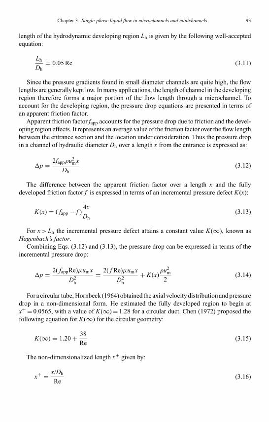
Kandlikar I044527-Ch03.tex 29/10/2005 9: 28 Page 93
Chapter 3. Single-phase liquid flow in microchannels and minichannels 93
length of the hydrodynamic developing region Lh is given by the following well-acceptedequation:
Lh
Dh= 0.05 Re (3.11)
Since the pressure gradients found in small diameter channels are quite high, the flowlengths are generally kept low. In many applications, the length of channel in the developingregion therefore forms a major portion of the flow length through a microchannel. Toaccount for the developing region, the pressure drop equations are presented in terms ofan apparent friction factor.
Apparent friction factor fapp accounts for the pressure drop due to friction and the devel-oping region effects. It represents an average value of the friction factor over the flow lengthbetween the entrance section and the location under consideration. Thus the pressure dropin a channel of hydraulic diameter Dh over a length x from the entrance is expressed as:
p = 2fappρu2mx
Dh(3.12)
The difference between the apparent friction factor over a length x and the fullydeveloped friction factor f is expressed in terms of an incremental pressure defect K(x):
K(x) = ( fapp − f )4x
Dh(3.13)
For x>Lh the incremental pressure defect attains a constant value K(∞), known asHagenbach’s factor.
Combining Eqs. (3.12) and (3.13), the pressure drop can be expressed in terms of theincremental pressure drop:
p = 2( fappRe)µumx
D2h
= 2( f Re)µumx
D2h
+ K(x)ρu2
m
2(3.14)
For a circular tube, Hornbeck (1964) obtained the axial velocity distribution and pressuredrop in a non-dimensional form. He estimated the fully developed region to begin atx+ = 0.0565, with a value of K(∞) = 1.28 for a circular duct. Chen (1972) proposed thefollowing equation for K(∞) for the circular geometry:
K(∞) = 1.20 + 38
Re(3.15)
The non-dimensionalized length x+ given by:
x+ = x/Dh
Re(3.16)

Kandlikar I044527-Ch03.tex 29/10/2005 9: 28 Page 94
94 Heat transfer and fluid flow in minichannels and microchannels
ac � 0.5
ac � 1.0
100101
x� � (x/Dh)/Re102103
101
102
f app
Re
ac � 0.2
ac 0.1
Fig. 3.3. Apparent friction factors for rectangular ducts in the developing region for different aspect ratios(α= 1/αc), Phillips (1987).
Shah and London (1978) showed that the frictional pressure drop in the developingregion of a circular duct obtained by Hornbeck (1964) can be accurately described by thefollowing equation:
p
(1/2)ρu2m
= 13.74(x+)1/2 + 1.25 + 64x+ − 13.74(x+)1/2
1 + 0.00021(x+)−2 (3.17)
Rectangular geometries are of particular interest in microfluidics applications. Shahand London (1978) and Kakac et al. (1987) present comprehensive summaries of theavailable literature. Phillips (1987) reviewed the available information, including that byCurr et al. (1972) and compiled the results for the apparent friction factor in a rectangularduct as shown in Fig. 3.3. It can be seen that fully developed flow is attained at different x+values, with low aspect ratio ducts reaching it earlier. The constant in Eq. (3.11) is around1 (x+ = 100) for rectangular ducts as seen from Fig. 3.3. Table 3.2 derived from Phillips(1987) gives the values of the apparent friction factor in a tabular form.
For other channel aspect ratios, a linear interpolation is suggested. Alternatively, usethe curve-fit equations provided in Appendix A.
The results for the fully developed friction factors and Hagenbach’s factors in trapezoidalchannels are reported by Kakac et al. (1987). By considering the rectangular channels as asubset of the trapezoidal geometry, Steinke and Kandlikar (2005a) obtained the followingcurve-fit equation for the Hagenbach’s factor for rectangular channels:
K(∞) = 0.6796 + 1.2197αc + 3.3089α2c − 9.5921α3
c
+ 8.9089α4c − 2.9959α5
c (3.18)

Kandlikar I044527-Ch03.tex 29/10/2005 9: 28 Page 95
Chapter 3. Single-phase liquid flow in microchannels and minichannels 95
Table 3.2Laminar flow friction factor in the entrance region of rectangular ducts.
fappRe
αc ≤ 0.1x+ = (x/Dh)/Re αc = 1.0 αc = 0.5 αc = 0.2 αc ≥ 10
0 142.0 142.0 142.0 287.00.001 111.0 111.0 111.0 112.00.003 66.0 66.0 66.1 67.50.005 51.8 51.8 52.5 53.00.007 44.6 44.6 45.3 46.20.009 39.9 40.0 40.6 42.10.01 38.0 38.2 38.9 40.40.015 32.1 32.5 33.3 35.60.02 28.6 29.1 30.2 32.40.03 24.6 25.3 26.7 29.70.04 22.4 23.2 24.9 28.20.05 21.0 21.8 23.7 27.40.06 20.0 20.8 22.9 26.80.07 19.3 20.1 22.4 26.40.08 18.7 19.6 22.0 26.10.09 18.2 19.1 21.7 25.80.10 17.8 18.8 21.4 25.60.20 15.8 17.0 20.1 24.7>1.0 14.2 15.5 19.1 24.0
For intermediate values use the curve-fit equations provided in Appendix A atthe end of the chapter.
The analysis presented in this section assumes a uniform velocity profile at the entranceof the channel. In many microfluidic applications, the channels have the manifold surfacesflush with the two opposing channel surfaces. The effect of such an arrangement was inves-tigated numerically by Gamrat et al. (2004). They showed that the resulting apparent fric-tion factors in the entrance region could be up to 50% lower than the theoretical predictions.
3.2.4. Fully developed and developing turbulent flow
A number of correlations with comparable accuracies are available in literature for fullydeveloped turbulent flow in smooth channels. The following equation by Blasius is usedextensively:
f = 0.0791 Re−0.25 (3.19)
A more accurate equation was presented by Phillips (1987) to cover both the developingand fully developed flow regions. He presented the fanning friction factor for a circulartube in terms of the following equation:
fapp = AReB (3.20)
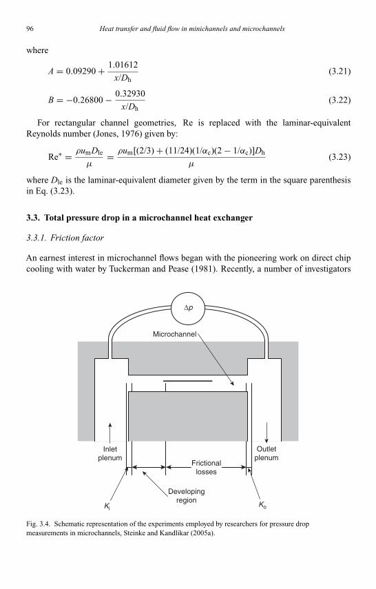
Kandlikar I044527-Ch03.tex 29/10/2005 9: 28 Page 96
96 Heat transfer and fluid flow in minichannels and microchannels
where
A = 0.09290 + 1.01612
x/Dh(3.21)
B = −0.26800 − 0.32930
x/Dh(3.22)
For rectangular channel geometries, Re is replaced with the laminar-equivalentReynolds number (Jones, 1976) given by:
Re∗ = ρumDle
µ= ρum[(2/3) + (11/24)(1/αc)(2 − 1/αc)]Dh
µ(3.23)
where Dle is the laminar-equivalent diameter given by the term in the square parenthesisin Eq. (3.23).
3.3. Total pressure drop in a microchannel heat exchanger
3.3.1. Friction factor
An earnest interest in microchannel flows began with the pioneering work on direct chipcooling with water by Tuckerman and Pease (1981). Recently, a number of investigators
KiKo
Developingregion
Inletplenum
Outletplenum
Microchannel
∆p
Frictionallosses
Fig. 3.4. Schematic representation of the experiments employed by researchers for pressure dropmeasurements in microchannels, Steinke and Kandlikar (2005a).

Kandlikar I044527-Ch03.tex 29/10/2005 9: 28 Page 97
Chapter 3. Single-phase liquid flow in microchannels and minichannels 97
including Li et al. (2000), Celata et al. (2002) and Steinke and Kandlikar (2005a) criticallyevaluated the available literature and presented explanations for the large deviations fromthe classical theory reported by some of the researchers.
A schematic representation of the pressure drop experiments conducted by theresearchers is shown in Fig. 3.4. Since measuring the local pressure along the flow isdifficult in microchannels, researchers have generally measured the pressure drop acrossthe inlet and outlet manifolds. The resulting pressure drop measurement represents thecombined effect of the losses in the bends, entrance and exit losses, developing regioneffects, and the core frictional losses. Thus, the measured pressure drop is the sum of thesecomponents (Phillips, 1987):
p = ρu2m
2
[(Ac/Ap)2(2K90) + (Kc + Ke) + 4fappL
Dh
](3.24)
where Ac and Ap are the total channel area and the total plenum cross-sectional area, K90is the loss coefficient at the 90 degree bends, Kc and Ke represent the contraction andexpansion loss coefficients due to area changes, and fapp includes the combined effects offrictional losses and the additional losses in the developing flow region. Phillips (1987)studied these losses and recommends K90 to be approximately 1.2. The contraction and exitlosses can be read from Fig. 3.5 derived from Kays and London (1984) and Phillips (1990).
1.31.21.11.00.90.80.70.60.50.40.30.20.10.0
0.0 0.1 0.2 0.3 0.4 0.5 0.6 0.7 0.8Area ratio, s
Kc
and
Ke
Kc
and
Ke
(a)0.9 1.0
�0.1�0.2�0.3�0.4�0.5�0.6�0.7�0.8
1.31.21.11.00.90.80.70.60.50.40.30.20.10.0
0.0 0.1 0.2 0.3 0.4 0.5 0.6 0.7 0.8Area ratio, s(b)
0.9 1.0
�0.1�0.2�0.3�0.4�0.5�0.6�0.7�0.8
4(L /D)/Re � � 0.20 � 0.10 � 0.05
4(L/D)/Re � 0.05 � 0.10 � 0.20
Re � 10,000 5000 3000
Re � 3000 5000 10,000
Re � 2000 10,000 ∞
KeRe � 10,0002000
Laminar
KcLaminar
KcLaminar
KcTurbulent
KeTurbulent
Ke Laminar
Fig. 3.5. Contraction and expansion loss coefficients for flow between inlet and outlet manifolds and themicrochannels, Kays and London (1984).

Kandlikar I044527-Ch03.tex 29/10/2005 9: 28 Page 98
98 Heat transfer and fluid flow in minichannels and microchannels
0.5
1.0
1.5
2.0
2.5
3.0
3.5
4.0
0 200 400 600 800Reynolds number, Re
C∗
UncorrectedCorrectedC∗ � 1.0
app
Fig. 3.6. Variation of C∗app = fapp,ex/fapp,th for a 200 µm square microchannel array after correcting for entrance
and exit losses.
Figure 3.5(a) is applicable to the low aspect ratio channels, αc < 0.1 and Fig. 3.5(b) is for0.1 ≤αc ≤ 1.0.
Equation (3.24) can also be written in terms of the fully developed friction factor f andthe pressure drop defect K(x):
p = ρu2m
2
[(Ac/Ap)2(2K90) + (Kc + Ke) + 4 f L
Dh+ K(x)
](3.25)
For L>Lh, K(x) is replaced by the Hagenbach’s factor K(∞) as discussed earlier inSection 3.2.3. Steinke and Kandlikar (2005a) conducted experiments on square siliconmicrochannels with 200 µm sides and 10 mm in length, and analyzed the data in detail. Aparameter C∗ is introduced to represent the ratio of the experimental and theoretical appar-ent friction factors. Figure 3.6 shows the data before and after applying the correctionsin C∗ = fapp,ex/fapp,th, where the subscripts ex and th refer to experimental and theoreticalvalues respectively. The uncorrected data converges to within 30% of the theoretical pre-dictions after all corrections are applied. It is suspected that the high errors are due to slightvariations in the channel cross-sectional area over its length, different entrance conditions,and errors associated with interpolations during data reduction.
Figure 3.7 shows the excellent agreement between the laminar flow theory and experi-mental results obtained by Judy et al. (2002) in 15–150 µm round and square microchannelsmade of fused silica and stainless steel with distilled water, methanol and isopropanol.Similar agreement is seen in Fig. 3.8 by Bucci et al. (2004) in 172, 290 and 520 µmdiameter stainless steel circular tubes with water in the fully developed laminar flowregion.

Kandlikar I044527-Ch03.tex 29/10/2005 9: 28 Page 99
Chapter 3. Single-phase liquid flow in microchannels and minichannels 99
D � 30.5 �m, L /D � 2019f Re � 64
D � 51.9 �m, L /D � 2192D � 97.9 �m, L /D � 2983f Re � 64
0 400 800 1200 1600 2000
0 200 400 600 800
Re
f Re
40
50
60
70
60
50
40
70
D � 77.6 �m, L /D � 3926D � 148.6 �m, L /D � 2030
D � 21.7 �m, L /D � 2341D � 40.1 �m, L /D � 2532
Fig. 3.7. Comparison between theory and experimental data of Judy et al. (2002) in 50–150 µm circular andsquare microchannels in the fully developed laminar region. (Note: f in this figure represents the Darcy frictionfactor, which is four times the Fanning friction factor used elsewhere in this text.)
1
0.1
f [�
]
100 1000
Re[�]
D � 172 �mD � 290 �mD � 520 �m64/Re
Fig. 3.8. Comparison between theory and experimental data of Bucci et al. (2004) in 171–520 µm diametercircular tubes in the fully developed laminar region. (Note: f in this figure represents the Darcy friction factor,which is four times the Fanning friction factor used elsewhere in this text.)
Niklas and Favre-Marinet (2003) analyzed the flow of water in a network of triangularmicrochannels with Dh = 110 µm. The contributions due to various losses were carefullyanalyzed in both their numerical as well as experimental work. They concluded that theclassical theory is applicable to modeling the flow through the entire system.

Kandlikar I044527-Ch03.tex 29/10/2005 9: 28 Page 100
100 Heat transfer and fluid flow in minichannels and microchannels
Another point that needs to be emphasized is the large errors that are associatedwith microscale experiments as pointed out by Judy et al. (2002). A detailed analysis wasconducted by Steinke and Kandlikar (2005a) for rectangular microchannels using actualmeasured parameters. Their final expression for uncertainty in estimating the product f Refor rectangular channels is given by:
Uf Re
f Re=[
2(
Uρ
ρ
)2
+(
Uµ
µ
)2
+(
Up
p
)2
+(
UL
L
)2
+ 3(
UQ
Q
)2
+ 5(
Ua
a
)2
+ 5(
Ub
b
)2
+ 2(
Ua
a + b
)2
+ 2(
Ub
a + b
)2]1/2
(3.26)
The details of the derivation are given by Steinke (2005). Note that the uncertainties inthe height a and width b measurements have a major influence on the overall uncertainty,followed by the uncertainties in the density and volumetric flow rate measurements. Thelow flow Reynolds number data in Fig. 3.6 exhibits extremely large uncertainties due tothe errors associated with the flow rate measurement. The large discrepancy reported inliterature by some of the earlier investigators is the result of the uncertainties in channeldimensions and flow rate measurements, entrance and exit losses, and the developingregion effects.
Figure 3.9 shows a picture of a microchannel cross-section obtained with a scanningelectron microscope by Steinke and Kandlikar (2005a). Note that the actual channel profile
G01-008a � 200 �mb � 250 �ms � 100 �m
54.3 �m33.9 �m
20 �m EHT � 20.00 kVWD � 6 mm
l Probe � 50 pAStage at T � 90.0°
Mag � 670 x
� 85.1 Deg
Date: 1 Apr 2005 Time: 17:02:39File Name � G01-008_003.tif
193.6 �m 93.9 �m
244.2 �m
Fig. 3.9. Cross-sectional view of a rectangular microchannels etched in silicon showing distortion in channelgeometry from ideal rectangular profile, Steinke and Kandlikar (2005a).

Kandlikar I044527-Ch03.tex 29/10/2005 9: 28 Page 101
Chapter 3. Single-phase liquid flow in microchannels and minichannels 101
deviates significantly from the intended rectangular profile. The side walls are undercut byabout 20 µm and the corners are rounded. This illustrates the need to accurately measurethe flow area and the for estimating the pressure drop characteristics of microchannels.
Similar conclusions were reached by other investigators, for example, Li et al. (2000),Celata (2002), Judy et al. (2002), Baviere et al. (2004), and Tu and Hrnjak (2003). Theincreasing deviations from the theoretical values at higher Reynolds numbers in manydata sets reported in literature is believed to be due to the increased length of the devel-oping region. Baviere and Ayela (2004) measured the local pressures along the flow in amicrochannel of height 7.5 µm. The range of Reynolds numbers considered was between0.1 and 15. Their results were found to agree with the classical theory. They also identifiedthe errors associated with the channel height measurement as being the largest source ofuncertainty.
Baviere et al. (2004) conducted experiments with bronze, altuglas, and silicon coatedmicrochannels with channel heights between 7.1 and 300 µm and channel widths between1 and 25 mm. Their results were also in excellent agreement with the classical theory.
Other effects that may influence the flow in microchannels are (i) high viscous dissi-pation causing a change in the fluid viscosity at the wall, and (ii) electrokinetic effects,which are covered in Chapter 4. The effect of viscous dissipation is reviewed by Shenet al. (2004). Xu et al. (2000) modeled this effect and found that the velocity profile wasmodified due to the viscous dissipation. The resulting friction factors were predicted to belower due to a reduction in the viscosity at higher liquid temperatures. The viscous effectwas studied experimentally by Judy et al. (2002). Their pressure drop data correlated wellwith the theory when they used the average of the inlet and outlet fluid temperatures fromtheir stainless steel microtubes, which were 15–100 µm in diameter. Koo and Kleinstreuer(2004) concluded that viscous dissipation effects increase rapidly with a decrease in thechannel dimensions and hence should be considered along with the imposed heat sourcesat the channel walls.
Figure 3.10 shows a plot of the friction factor versus Reynolds number using the exper-imental data points reported in literature as compiled by Steinke and Kandlikar (2005a).The lines represent the theoretical values for different channel aspect ratios. These datapoints were screened to eliminate the data that were obtained with large uncertainties andthose which did not account for the entrance and exit losses. It is seen that the generaltrends are followed, though the errors are still quite large mainly due to the uncertaintiesassociated with channel size measurement.
3.3.2. Laminar-to-turbulent transition
The laminar-to-turbulent flow transition is another topic that was analyzed by a number ofinvestigators. The laminar-to-turbulent transition in abrupt entrance rectangular ducts wasfound to occur at a transition Reynolds number of Ret = 2200 for αc = 1 and at Ret = 2500(Hartnett et al., 1962) for parallel plates with αc = 0. For other aspect ratios, a linearinterpolation between these two values is recommended.
Some of the initial studies indicated an early transition to turbulent flow in microchan-nels. However, a number of recent studies showed that the laminar-to-turbulent transition

Kandlikar I044527-Ch03.tex 29/10/2005 9: 28 Page 102
102 Heat transfer and fluid flow in minichannels and microchannels
1E�04
1E�03
1E�02
1E�01
1E�00
1E�01
1E�02
1E�03
1E�04
1E�05
1E�03 1E�01 1E�01 1E�03 1E�05Reynolds number, Re
Fric
tion
fact
or,
f
f Re � 24 f Re � 16f Re � 14Data
Fig. 3.10. Comparison of friction factors reported in literature with the theoretical values for differentmicrochannel geometries. Entrance and exit losses and the developing region at the entrance were notaccounted for in a number of data sets reviewed by Steinke and Kandlikar (2005a).
remains unchanged. Figure 3.8 by Bucci et al. (2004) shows that the transition occurredaround Ret = 2000 for circular microtubes 171–520 µm in diameter. The results of Baviereet al. (2004) also indicate that the laminar-to-turbulent transition in smooth microchannelsis not influenced by the channel dimensions and occurs around 2300. Similar results werereported by a number of investigators, including Bucci et al. (2004), Schmitt and Kandlikar(2005), Kandlikar et al. (2005) for minichannels with Dh < 1 mm; and Li et al. (2000) for80 µm ≤ Dh ≤ 166.3 µm.
The transition from the laminar-to-turbulent region is influenced by the channel surfaceroughness. Further details of this effect are discussed in the next section on roughness.
3.4. Roughness effects
3.4.1. Roughness representation
Darcy (1857) investigated the effects of surface roughness on the turbulent flow of water inrough pipes made of cast iron, lead, wrought iron, and asphalt-covered cast iron. The pipeswere 12 to 500 mm in diameter and 100 m long. Fanning (1886) proposed a correlation forthe pressure drop as a function of roughness. Mises (1914) is credited with introducing theterm relative roughness, which was originally defined as the ratio of absolute roughnessto the pipe radius (we now use pipe diameter to normalize roughness parameters, suchas average roughness Ra). Nikuradse (1933) presented a comprehensive review of theliterature covering uniform roughness and roughness structures such as corrugations, and
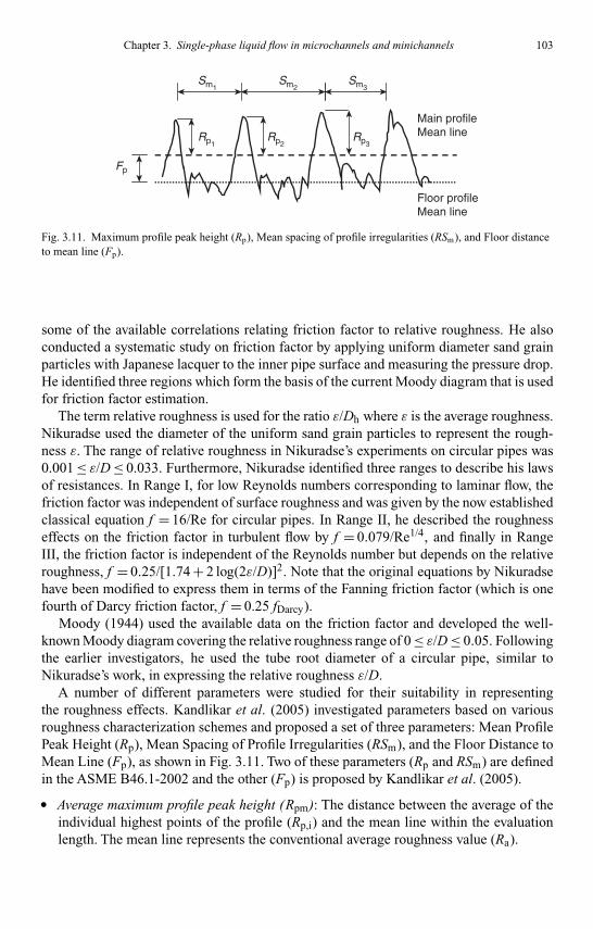
Kandlikar I044527-Ch03.tex 29/10/2005 9: 28 Page 103
Chapter 3. Single-phase liquid flow in microchannels and minichannels 103
Floor profileMean line
Fp
Main profileMean line
Sm1
Rp1Rp2
Rp3
Sm2Sm3
Fig. 3.11. Maximum profile peak height (Rp), Mean spacing of profile irregularities (RSm), and Floor distanceto mean line (Fp).
some of the available correlations relating friction factor to relative roughness. He alsoconducted a systematic study on friction factor by applying uniform diameter sand grainparticles with Japanese lacquer to the inner pipe surface and measuring the pressure drop.He identified three regions which form the basis of the current Moody diagram that is usedfor friction factor estimation.
The term relative roughness is used for the ratio ε/Dh where ε is the average roughness.Nikuradse used the diameter of the uniform sand grain particles to represent the rough-ness ε. The range of relative roughness in Nikuradse’s experiments on circular pipes was0.001 ≤ ε/D ≤ 0.033. Furthermore, Nikuradse identified three ranges to describe his lawsof resistances. In Range I, for low Reynolds numbers corresponding to laminar flow, thefriction factor was independent of surface roughness and was given by the now establishedclassical equation f = 16/Re for circular pipes. In Range II, he described the roughnesseffects on the friction factor in turbulent flow by f = 0.079/Re1/4, and finally in RangeIII, the friction factor is independent of the Reynolds number but depends on the relativeroughness, f = 0.25/[1.74 + 2 log(2ε/D)]2. Note that the original equations by Nikuradsehave been modified to express them in terms of the Fanning friction factor (which is onefourth of Darcy friction factor, f = 0.25 fDarcy).
Moody (1944) used the available data on the friction factor and developed the well-known Moody diagram covering the relative roughness range of 0 ≤ ε/D ≤ 0.05. Followingthe earlier investigators, he used the tube root diameter of a circular pipe, similar toNikuradse’s work, in expressing the relative roughness ε/D.
A number of different parameters were studied for their suitability in representingthe roughness effects. Kandlikar et al. (2005) investigated parameters based on variousroughness characterization schemes and proposed a set of three parameters: Mean ProfilePeak Height (Rp), Mean Spacing of Profile Irregularities (RSm), and the Floor Distance toMean Line (Fp), as shown in Fig. 3.11. Two of these parameters (Rp and RSm) are definedin the ASME B46.1-2002 and the other (Fp) is proposed by Kandlikar et al. (2005).
● Average maximum profile peak height (Rpm): The distance between the average of theindividual highest points of the profile (Rp,i) and the mean line within the evaluationlength. The mean line represents the conventional average roughness value (Ra).

Kandlikar I044527-Ch03.tex 29/10/2005 9: 28 Page 104
104 Heat transfer and fluid flow in minichannels and microchannels
● Mean spacing of profile irregularities ( RSm): Consists of the mean value of the spacingbetween profile irregularities within the evaluation length. The irregularities of interestare the peaks, so this is equivalent to the Pitch.
RSm = 1
n
n∑i=1
Smi (3.27)
● Floor distance to mean line (Fp): Consists of the distance between the main profilemean line (determined by Ra) and the floor profile mean line. The floor profile is theportion of the main profile that lies below the main profile mean line.
The three parameters described above allow the characterization of the peak height,peak spacing and the distance from the floor to the mean line. These parameters will definethe characteristics of the surface roughness that influence the location and shape of thefluid flow streamlines (as described by Webb et al., 1971 and Kandlikar et al., 2005)and, consequently, the size of the recirculation flow zones between roughness elements.From the above parameters, the equivalent roughness ε can be estimated by the followingrelationship:
ε = Rpm + Fp (3.28)
For the sand grain roughness employed by Nikuradse, the new definition of roughnessε yields the same value, and hence no correction is needed for any of the friction factorcorrelations and charts. The use of mean spacing between profile irregularities is expectedto represent the structured roughness surfaces. Such surfaces may be designed in the futureto obtain specific pressure drop and heat transfer performance characteristics.
3.4.2. Roughness effect on friction factor
For microchannels, the relative roughness values are expected to be higher than the limitof 0.05 used in the Moody diagram. Kandlikar et al. (2005) considered the effect of cross-sectional area reduction due to protruding roughness elements and recommended usingthe constricted flow area in calculating the friction factor. Using a constricted diameterDcf = D − 2ε, a modified Moody diagram was presented as shown in Fig. 3.12. In theturbulent region, it was found that such a representation yielded a constant value of frictionfactor above ε/Dcf > 0.03.
In the turbulent fully rough region, 0.03 ≤ ε/Dcf ≤ 0.05, the friction factor based on theconstricted flow diameter is given by:
f Darcy,cf = 0.042 (3.29a)
In terms of the Fanning friction factor, we get:
fcf = fDarcy,cf /4 = 0.042/4 = 0.0105 (3.29b)
Since experimental data is not available beyond ε/Dcf > 0.05, using Eq. (3.29) for higherrelative roughness values than 0.05 is not recommended. Note that the friction factor and

Kandlikar I044527-Ch03.tex 29/10/2005 9: 28 Page 105
Chapter 3. Single-phase liquid flow in microchannels and minichannels 105
0.01
0.10
1E�02 1E�03 1E�04 1E�05 1E�06 1E�07 1E�08
Reynolds number based upon constricted flow, Recf
Fric
tion
fact
or b
ased
on
cons
tric
ted
flow
, fD
arcy
,cf
Lam
inar
flow
f cf =
64/
Re c
f
Tra
nsiti
onzo
ne
Smooth pipe0.00025
0.0005
0.001
0.002
0.0040.0060.0080.0100.0140.020
Rel
ativ
e ro
ughn
ess,
ε/D
cf
0.02
0.03
0.04
0.05
0.06
0.07
0.080.09
Plateau
0.030
Fig. 3.12. Darcy friction factor plot based on a constricted flow diameter, Kandlikar et al. (2005).
the geometrical and flow parameters are based on the constricted flow diameter as givenby the following equations:
Dcf = D − 2ε (3.30)
p = 2fcfρu2m,cf L
Dh,cf(3.31)
um,cf = m/Acf (3.32)
Recf = ρum,cf Dh,cf
µ(3.33)
In the fully developed laminar flow region, the constricted friction factor is given bythe following equation, Kandlikar et al. (2005):
Laminar region, 0 ≤ ε/Dh,cf ≤ 0.15;
fcf = Po
Recf(3.34)
where the Poiseuille number Po is given by either Eq. (3.9) or (3.10) depending on the chan-nel geometry. In the turbulent region, use the modified Miller equation as recommendedby Kandlikar et al. (2005).
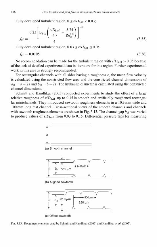
Kandlikar I044527-Ch03.tex 29/10/2005 9: 28 Page 106
106 Heat transfer and fluid flow in minichannels and microchannels
Fully developed turbulent region, 0 ≤ ε/Dh,cf < 0.03;
fcf =0.25
[log10
(ε/Dh,cf
3.7+ 5.74
Re0.9cf
)]
4
−2
(3.35)
Fully developed turbulent region, 0.03 ≤ ε/Dh,cf ≤ 0.05
fcf = 0.0105 (3.36)
No recommendation can be made for the turbulent region with ε/Dh,cf > 0.05 becauseof the lack of detailed experimental data in literature for this region. Further experimentalwork in this area is strongly recommended.
For rectangular channels with all sides having a roughness ε, the mean flow velocityis calculated using the constricted flow area and the constricted channel dimensions ofacf = a − 2ε and bcf = b − 2ε. The hydraulic diameter is calculated using the constrictedchannel dimensions.
Schmitt and Kandlikar (2005) conducted experiments to study the effect of a largerelative roughness of ε/Dh,cf up to 0.15 in smooth and artificially roughened rectangu-lar minichannels. They introduced sawtooth roughness elements in a 10.3 mm wide and100 mm long test channel. Cross-sectional views of the smooth channels and channelswith sawtooth roughness elements are shown in Fig. 3.13. The channel gap bcf was variedto produce values of ε/Dh,cf from 0.03 to 0.15. Differential pressure taps for measuring
(a) Smooth channel
(b) Aligned sawtooth
72.9 �m
72.9 �m
(c) Offset sawtooth
250 �m
b
b
b
500 �m
500 �m
bcf
bcf
Fig. 3.13. Roughness elements used by Schmitt and Kandlikar (2005) and Kandlikar et al. (2005).

Kandlikar I044527-Ch03.tex 29/10/2005 9: 28 Page 107
Chapter 3. Single-phase liquid flow in microchannels and minichannels 107
the local pressure drops were located at several locations along the flow length in the fullydeveloped region.
The smooth channel results reported by Kandlikar et al. (2005) closely follow the clas-sical laminar flow theory for friction factor. The experimental data from the two sawtoothstructures are represented in Fig. 3.14 for flow of water with b = 500 µm, resulting ina Dh of 953 µm. This plot uses the height b in calculating Dh and Re. The dashed linerepresents the f Re = Constant line corresponding to the channel aspect ratio αc = a/b. Itis seen that the agreement in the low Reynolds number region corresponding to laminarflow is considerably off.
Figure 3.15 shows the same data used in Fig. 3.14, but plotted with the constrictedflow areas and using the constricted flow parameters given by Eqs. (3.30)–(3.33). The
0.01
0.10
1.00
100 1000 10,000Re
f
Lam., theory Turb., theory-extendedAligned sawtooth Offset sawtooth
Fig. 3.14. Fully developed friction factor versus Reynolds number, both based on hydraulic diameter for waterflow. Dh = 953 µm, b = 500 µm, bcf = 354 µm, w= 10.03 mm, ε/Dh = 0.0735, Kandlikar et al. (2005).
0.001
0.010
0.100
1.000
100 1000 10,000Recf
f cf
Lam., theory Turb., theory-extendedConstricted aligned sawtooth Constricted offset sawtooth
Fig. 3.15. Fully developed friction factor versus Reynolds number, both based on constricted flow hydraulicdiameter; water flow. Dh,cf = 684 µm, b = 500 µm, bcf = 354 µm, w= 10.03 mm, ε/Dh,cf = 0.1108, Kandlikaret al. (2005).

Kandlikar I044527-Ch03.tex 29/10/2005 9: 28 Page 108
108 Heat transfer and fluid flow in minichannels and microchannels
results shown in Fig. 3.15 in the laminar region show good agreement with the acceptedlaminar flow theory ( fcf Recf = Constant). Similar results were obtained for different gapsizes (yielding different relative roughness values) for both the offset sawtooth and alignedsawtooth geometries.
3.4.3. Roughness effect on the laminar-to-turbulent flow transition
The transition from laminar-to-turbulent flow has been reported to occur in microchannelsat Reynolds numbers considerably below 2300. In many experiments, the transition hasbeen mistakenly identified to occur early based on experimental data uncorrected forthe developing length (Steinke and Kandlikar, 2005a). Kandlikar et al. (2003) conductedexperiments with stainless steel tubes and noted that early transition occurred for a 0.62 mmID stainless steel tube with a surface roughness ε/Dh of 0.355%. Schmitt and Kandlikar(2005) conducted careful experiments with plain and sawtooth roughened channels withair and water. Their results for smooth rectangular channels showed a transition Reynoldsnumber between 2000 and 2300, but for increasing relative roughness values there wasa decreasing transition Reynolds numbers as seen in Figs. 3.14 and 3.15. Figure 3.16shows the transition Reynolds number as a function of the relative roughness (based on theconstricted hydraulic diameter). The following equations are used to describe the roughnesseffects based on their experimental data.
Laminar-to-turbulent transition criteria:
For 0 < ε/Dh,cf ≤ 0.08: Ret,cf = 2300 − 18,750(ε/Dh,cf ) (3.37)
For 0.08 < ε/Dh,cf ≤ 0.15: Ret,cf = 800 − 3270(ε/Dh,cf − 0.08) (3.38)
0
500
1000
1500
2000
2500
0 0.05 0.1 0.15ε/Dh,cf
Re c
f
AirWater
Fig. 3.16. Transition Reynolds number variation with relative roughness based on constricted flow diameter,Equations (3.37) and (3.38) plotted along with data from Schmitt and Kandlikar (2005).
Kandlikar I044527-Ch03.tex 29/10/2005 9: 28 Page 109
Chapter 3. Single-phase liquid flow in microchannels and minichannels 109
Friction factor in the transition region for rough tubes with ε/Dh,cf ≤ 0.05 at a givenRecf can be obtained by a linear interpolation of (i) the laminar friction factor obtainedfrom Eq. (3.34) at the transition Reynolds number, and (ii) the turbulent friction fac-tor at Recf = 2300 given by Eq. (3.35) or (3.36) depending on the value of ε/Dh,cf . Forε/Dh,cf > 0.05 in the transition region, additional experimental data is needed before anyrecommendations can be made.
3.4.4. Developing flow in rough tubes
Developing flow in rough tubes has not been explored in literature. As a preliminaryestimate, the methods described in Section 3.2.3 for smooth tubes are recommended byintroducing the constricted flow diameter in calculating the flow velocity, Reynolds numberand friction factor. Further research in this area is needed.
3.5. Heat transfer in microchannels
3.5.1. Fully developed laminar flow
The Nusselt number in fully developed laminar flow is expected to be constant as predictedby the classical theory. However, there are a number of investigations reported in literaturethat show a trend increasing with Reynolds number in this range. This results from theexperimental uncertainties as discussed in Section 3.5.3.
The Nusselt number in the fully developed laminar flow is constant and depends onthe channel geometry and the wall heat transfer boundary condition. Table 3.1 presentsthe Nusselt numbers for commonly used geometries under constant heat flux and constantwall temperature boundary conditions.
For a rectangular channel, the Nusselt number depends on the channel aspect ratioαc = a/b, and the wall boundary conditions. Three boundary conditions are identified inliterature and the Nusselt number for each one is given below.
Constant wall temperature, T-boundary condition:
NuT = 7.541(1 − 2.610αc + 4.970α2c − 5.119α3
c + 2.702α4c − 0.548α5
c) (3.39)
Constant circumferential wall temperature, uniform axial heat flux, H1 boundarycondition:
NuH1 = 8.235(1 − 2.0421αc + 3.0853α2c − 2.4765α3
c
+ 1.0578α4c − 0.1861α5
c) (3.40)
Constant wall heat flux, both circumferentially and axially:
NuH2 = 8.235(1 − 10.6044αc + 61.1755α2c − 155.1803α3
c
+ 176.9203α4c − 72.9236α5
c) (3.41)

Kandlikar I044527-Ch03.tex 29/10/2005 9: 28 Page 110
110 Heat transfer and fluid flow in minichannels and microchannels
Table 3.3Fully developed laminar flow Nusselt numbers.
αc = a/b Nufd,3 Nufd,4
0 8.235 8.2350.10 6.939 6.7000.20 6.072 5.7040.30 5.393 4.9690.40 4.885 4.4570.50 4.505 4.1110.70 3.991 3.7401.00 3.556 3.5991.43 3.195 3.7402.00 3.146 4.1112.50 3.169 4.4573.33 3.306 4.9695.00 3.636 5.70410.00 4.252 6.700>10.00 5.385 8.235
a – unheated side in three-side heated case.For intermediate values, use the curve-fit equations provided inAppendix A at the end of the chapter.
In reality, all practical situations fall somewhere in the middle of these three bound-ary conditions. This becomes an especially important issue in the case of microchannelsbecause of the difficulty in identifying a correct boundary condition with discretly spacedheat sources, and two-dimensional effects in the base and the fins.
The heating in microchannel geometries generally comes from three sides, as a coverof glass or some other material is bonded on top of the microchannels to form the flowpassages. The fully developed Nusselt numbers for both three- and four-side heated ductshave been compiled from various sources, including Wibulswas (1966), and Phillips (1987)and are given inTable 3.3. Note that the side with dimension a is not heated, and the channelaspect ratio is defined as αc = a/b.
3.5.2. Thermally developing flow
The thermal entry length is expressed by the following form for flow in ducts:
Lt
Dh= c Re Pr (3.42)
For circular channels, the leading constant c in Eq. (3.42) is found to be 0.05, while forrectangular channels, the plots presented by Phillips (1987) suggest c = 0.1.
The local heat transfer in the developing region of a circular tube is given by the followingequations (Shah and London, 1978):
Nux = 4.363 + 8.68(103 x∗)−0.506e−41x∗(3.43)

Kandlikar I044527-Ch03.tex 29/10/2005 9: 28 Page 111
Chapter 3. Single-phase liquid flow in microchannels and minichannels 111
Table 3.4Thermal entry region Nusselt numbers.
Nux,4
x* αc ≤ 0.1* αc = 0.25 αc = 0.333 αc = 0.5 αc = 1.0 αc ≥ 10**
0.0001 31.4 26.7 27.0 23.7 25.2 31.60.0025 11.9 10.4 9.9 9.2 8.9 11.20.005 10 8.44 8.02 7.46 7.1 9.00.00556 9.8 8.18 7.76 7.23 6.86 8.80.00625 9.5 7.92 7.5 6.96 6.6 8.50.00714 9.3 7.63 7.22 6.68 6.32 8.20.00833 9.1 7.32 6.92 6.37 6.02 7.90.01 8.8 7 6.57 6.05 5.69 7.490.0125 8.6 6.63 6.21 5.7 5.33 7.20.0167 8.5 6.26 5.82 5.28 4.91 6.70.025 8.4 5.87 5.39 4.84 4.45 6.20.033 8.3 5.77 5.17 4.61 4.18 5.90.05 8.25 5.62 5.00 4.38 3.91 5.550.1 8.24 5.45 4.85 4.22 3.71 5.41 8.23 5.35 4.77 4.11 3.6 5.38
x∗ = x/(Re PrDh); * – parallel plates, both sides heated; ** – parallel plates, one side heated.For intermediate values, use the curve-fit equations provided in Appendix A.
x∗ = x/Dh
Re Pr(3.44)
For rectangular channels with the four-side heating configuration, Nusselt numbers inthe thermally developing region presented in Table 3.4 are derived from Phillips’ (1987)work. For the three-side heating configuration the following scheme is suggested by Phillips(1990).
Three-side heating, αc ≤ 0.1 and αc ≥ 10, use four-side heating table without anymodification.
Three-side heating, 0.1<αc < 10:
Nux,3(x∗,αc) = Nux,4(x∗,αc)Nufd,3(x∗ = x∗
fd,αc)
Nufd,4(x∗ = x∗fd,αc)
(3.45)
The subscripts x, 3 and x, 4 refer to the location at a distance x in the heated length forthe three-sided and four-sided heating cases respectively. The Nusselt numbers in the fullydeveloped region for both heating configurations are obtained from Table 3.3, and in thedeveloping region Nusselt numbers for the four-sided heating are obtained from Table 3.4.
The use of fully developed hydrodynamic conditions in heat transfer analysis isreasonable for water. Garimella and Singhal (2004) noted that assuming fully developedhydrodynamic conditions and thermally developing conditions resulted in a satisfactoryagreement with their data for microchannels.

Kandlikar I044527-Ch03.tex 29/10/2005 9: 28 Page 112
112 Heat transfer and fluid flow in minichannels and microchannels
3.5.3. Agreement between theory and available experimental data onlaminar flow heat transfer
Laminar flow heat transfer in microchannels has been studied by a number of researchers.Agreement with the classical laminar flow theory is expected to hold, but the reported datashow significant scatter due to difficulties encountered in making accurate local heat fluxand temperature measurements. Steinke and Kandlikar (2005b) reviewed the availabledata and presented a comprehensive table showing the range of parameters employed.The laminar flow heat transfer in the fully developed region is expected to be constant, butthe data taken from literature show a generally linear increase in Nusselt number with flowReynolds number as seen in Fig. 3.17.
The main reasons for this discrepancy have been attributed to the following factors:
(i) Entrance region effects: The researchers have used the fully developed theoreticalvalues for Nusselt numbers in their comparison with the experimental data. Due tothe relatively short lengths employed in microchannels, the influence of the entranceregion cannot be neglected. The entrance region effects become more significant athigher Reynolds numbers, in part explaining the increasing Nusselt number trend withReynolds number as seen in Fig. 3.17.
(ii) Uncertainties in experimental measurements: The uncertainties in heat transfer mea-surements have been analyzed by a number of investigators, including Judy et al.(2002) and Steinke and Kandlikar (2005b). The following equation for the uncer-tainty in the Nusselt number calculation from the uncertainties in the experimentalmeasurements is presented by Steinke and Kandlikar for a rectangular channel of base
1E�01
1E�00
1E�01
1E�02
1E�03
1E�04
1E�00 1E�01 1E�02 1E�03 1E�04 1E�05Reynolds number, Re
Nus
selt
num
ber,
Nu
Fig. 3.17. Selected experimental data for single-phase liquid flow in microchannels and minichannels,Dh = 50 µm to 600 µm.

Kandlikar I044527-Ch03.tex 29/10/2005 9: 28 Page 113
Chapter 3. Single-phase liquid flow in microchannels and minichannels 113
width a and height b:
UNu = Nu ·[(
Ukf
kf
)2
+(
UI
I
)2
+(
UV
V
)2
+ 4(
UTs
Ts
)2
+ 2(
UTi
Ti
)2
+ 2(
UTo
To
)2
+ 3(
UL
L
)2
+ 4(
Ua
a
)2
+ 5(
Ub
b
)2
+ 2(
Uηf
ηf
)2]1/2
(3.46)
where I – current, V – voltage, Ts – surface temperature, Ti – fluid inlet temperature,To – fluid outlet temperature, L – flow length, a and b – cross-section dimensions, andηf – fin efficiency. The uncertainties in the measurement of the surface temperature andflow channel dimensions play a critical role in the overall uncertainty. The importanceof accurate geometrical measurements was emphasized in the friction factor estimationas well. Accurate surface temperature measurement poses a significant challenge dueto the small dimensions of the test section. Use of silicon chips with integrated circuitsto measure the temperatures is recommended.
Another factor that makes the temperature measurements critical in the overalluncertainty is the small temperature difference between the surface and the fluid atthe outlet. Since the heat transfer coefficients are very high in microchannels, and theflow is relatively low (low Reynolds number), the outlet temperature in many exper-iments approaches the surface temperature. Proper experiments need to be designedto account for this effect.
(iii) Ambiguity in the determination of the thermal boundary condition: Several exper-iments reported in literature were conducted with microchannels or minichannelsfabricated on copper or silicon substrates. The actual boundary conditions for thesetest sections are difficult to ascertain as they fall in between the constant temperatureand constant heat flux boundary conditions. Furthermore, in many cases the heatingis three-sided with the side walls acting as fins. The fin efficiency effects also alter theheat flux and temperature distributions. A clear comparison is only possible after theconjugate heat transfer effects are incorporated into a detailed numerical simulationof the test section.
3.5.4. Roughness effects on laminar flow heat transfer
Kandlikar et al. (2003) studied the heat transfer and pressure drop of laminar flow insmooth and rough stainless steel tubes of 1.067 and 0.62 mm ID. The surface roughnessof the inner tube wall was changed by treating it with two different acid mixtures. Thesurface roughness actually went down after the acid treatment as the protruding peaks inthe surface profile were smoothed out. The effect of changes in the relative roughnesson pressure drop was minimal, but the heat transfer in the entry region showed a distinctdependence on roughness. Figure 3.18 shows the local Nusselt number at a location 52 mmfrom the start of the heated length. The flow was hydrodynamically fully developed priorto entering the heated section.

Kandlikar I044527-Ch03.tex 29/10/2005 9: 28 Page 114
114 Heat transfer and fluid flow in minichannels and microchannels
02468
101214161820
0 500 1000 1500 2000 2500 3000Re
Nu
Nu(Twmid, e/d � 0.00355)
Nu(Twmid, e/d � 0.0029)
Nu(Twmid, e/d � 0.00161)
Fig. 3.18. The effect of roughness in the entrance region (x = 52 mm) of a 0.62 mm inner diameter tube with afully developed velocity profile and a developing temperature profile, Kandlikar et al. (2003).
It is seen from Fig. 3.18 that the Nusselt number increases even for a modest increase inthe relative roughness from 0.161% to 0.355%. Also note that the location where the heattransfer measurements were taken was preceded by a tube length longer than the hydraulicentry length, which was 380 mm at Re = 2300. A number of researchers did not correctlyidentify the developing region and have mistakenly reported the increasing trend in the Nuversus Re plot as being in the fully developed region.
It is not possible to present any equations for heat transfer enhancement with roughnessbecause of the lack of systematic data covering the entire region. Further research inthis area is strongly recommended. With structured roughness surfaces, the enhancementresults from the combined effects of area enhancement and that due to the flow modificationcaused by the roughness elements.
3.5.5. Heat transfer in the transition and turbulent flow regions
A detailed discussion was presented earlier on the critical Reynolds number for the laminar-to-turbulent transition. For smooth channels, the well-established criterion of Rec = 2300is expected to hold. The effect of roughness is described by Eqs. (3.32) and (3.33). Since thetransition region is encountered in many minichannel and microchannel heat exchangers,there is a need for generating accurate experimental data for both smooth and rough tubesin this region.
Phillips (1990) suggests using the following equations in the developing turbu-lent region. For larger values of x, the influence of the term [1 + (Dh/x)2/3] reducesasymptotically to 1:
For 0.5 < Pr < 1.5: Nu = 0.0214[1.0 + (Dh/x)2/3] [Re0.8 − 100]Pr0.4 (3.47)
For 1.5 < Pr < 500: Nu = 0.012[1.0 + (Dh/x)2/3] [Re0.87 − 280]Pr0.4 (3.48)
Further validation of these equations in microchannels is warranted. Adams et al.(1997) conducted experimental work in the turbulent region with flow of water in 0.76 and
Kandlikar I044527-Ch03.tex 29/10/2005 9: 28 Page 115
Chapter 3. Single-phase liquid flow in microchannels and minichannels 115
0.109 mm diameter circular channels. Based on their data, they proposed the followingequation that also matches the data by Yu et al. (1995) within ±18.6%:
Nu = NuGn(1 + F) (3.49)
where
NuGn = ( f /8)(Re − 1000)Pr
1 + 12.7( f /8)1/2(Pr2/3 − 1)(3.50)
f = (1.82 log(Re) − 1.64)−2 (3.51)
F = CRe(1 − (D/Do)2) (3.52)
NuGn represents the Nusselt number predicted by Gnielinski (1976) correlation. Theleast-squares fit to all the data sets studied byAdams et al. (1997) resulted in C = 7.6 × 10⁻⁵
and Do = 1.164 mm.Heat transfer coefficients in microchannels are very high due to their small hydraulic
diameters. The high pressure gradients have led researchers to employ low flow rates.However, with the reduced flow rate, the ability of the fluid stream to carry the heat awayfor a given temperature rise becomes limited. In order to improve the overall coolingperformance, the following two options are available.
(a) Reduce the flow length of the channels.(b) Increase the liquid flow rate.
As a result, employing multiple streams with short paths in a microchannel heatexchanger is recommended, similar to a split flow arrangement providing two streamsas will be discussed in Section 3.7. The reduced flow length will then enable the designerto employ higher flow rates under a given pressure drop limit. This scheme offers severaladvantages over a single-pass arrangement where the fluid traverses the entire length ofthe heat exchanger:
(i) The reduced flow length reduces the pressure drop: The short flow length effectivelyreduces the overall pressure drop.
(ii) Larger developing region: The multiple inlets result in a larger channel area beingunder developing conditions where the heat transfer is higher.
(iii) Higher flow velocities: Some of the pressure drop reduction could be used to increasethe flow velocity of individual streams. The possibility of employing turbulent flowshould also be explored as the heat transfer coefficient is higher in this region.
3.5.6. Variable property effects
The property ratio method is usually recommended in accounting for the property variationsdue to temperature changes in the heat exchanger flow passages. The following equationsare recommended for liquids:
f /fcp = [µw/µb]M (3.53)

Kandlikar I044527-Ch03.tex 29/10/2005 9: 28 Page 116
116 Heat transfer and fluid flow in minichannels and microchannels
Nu/Nucp = [µw/µb]N (3.54)
where the subscript cp refers to the constant property solution obtained from appropriateequations or correlations. For laminar flow, M = 0.58 and N = −0.14, and for turbulentflow, M = 0.25 and N = −0.11 (Kays and London, 1984).
3.6. Microchannel and minichannel geometry optimization
The first practical implementation of microchannels in silicon devices was demonstratedby Tuckerman and Pease (1981). They were able to dissipate 7.9 MW/m2 with a maxi-mum substrate temperature rise of 71◦C and a pressure drop of 186 kPa. The allowabletemperature differences and the pressure drops for cooling today’s microprocessor chipshave become significantly smaller, and many investigators have been working towardsoptimization of the channel geometrical configuration.
The application of microchannels to electronics cooling imposes severe design con-straints on the system design. For a given heat dissipation rate, the flow rate, pressuredrop, fluid temperature rise, and fluid inlet to surface temperature difference requirementsnecessitate optimization of the channel geometry. A number of investigators studied thegeometrical optimization of microchannel heat exchangers, For example, Phillips (1987),Harpole and Eninger (1991), Knight et al. (1992), Ryu et al. (2002), Bergles et al. (2003),and Kandlikar and Upadhye (2005). The results found by Kandlikar and Upadhye arepresented below.
Kandlikar and Upadhye (2005) considered a microchannel system as shown in Fig. 3.19.For a chip of width W = 10 mm and length L = 10 mm, they presented an analysis schemefor heat transfer and pressure drop by incorporating the entrance region effects. The numberof channels was used as a parameter in developing the optimization scheme. The maximumchip temperature was set at 360 K while the fluid inlet temperature was set equal to 300 K.The channel depth was assumed to be 200 µm.
Figures 3.20 and 3.21 show the parametric plots resulting from the optimization pro-gram. The fin spacing ratio, defined as β= s/a, is plotted as a function of the number ofchannels on a 10 mm wide chip with pressure drop, water flow rate and fin thickness asparameters. A lower limiting value of approximately 40 µm was considered achievable for
W
Cover plate
b
s La
Fig. 3.19. Microchannel geometry used in microprocessor heat sink channel size optimization, Kandlikar andUpadhye (2005).

Kandlikar I044527-Ch03.tex 29/10/2005 9: 28 Page 117
Chapter 3. Single-phase liquid flow in microchannels and minichannels 117
fin thickness using silicon microfabrication techniques. For a given pressure drop limit, theoptimal number of channels and other channel geometrical parameters can be determinedfrom this plot. Such plots could be generated for other system configurations as well.
The effect of introducing offset strip-fins in the microchannel flow passages and a splitflow arrangement, as shown in Figs. 3.22 and 3.23 respectively, was also analyzed by
50 600.2
0.3
0.4
0.5
0.6
1
0.9
0.8
0.7
70 80
40
30
30
50
6070
70
80
80
60
3025
30
45
3535
25
405055
45
4540
40
35
90 100Number of channels
Fin
spa
cing
rat
io
40
50
Fig. 3.20. Contour plot of fin spacing ratio β versus the number of channels with pressure drop across themin kPa (dash-dot lines) and fin thickness in µm (solid lines) as parameters for water flow in plain rectangularmicrochannels in a single-pass arrangement at a heat flux of 3 MW/m2, Kandlikar and Upadhye (2005).
1
0.9
0.8
0.7
Fin
spa
cing
rat
io
0.6
70
70
60
60
60
50
50
50
40
40
30
30
0.5
0.4
0.3
0.250 60 70 80
Number of channels90 100
1.75
1.75
2
2
3
1.25
1.25
1.1
1.0
1.25
1.75
1.5
1.5
2.5
2.5
80
Fig. 3.21. Contour plot of fin spacing ratio β versus the number of channels with water flow rate in 10−3 kg/s(dash-dot lines) and fin thickness in µm (solid lines) as parameters for water flow in plain rectangularmicrochannels in a single-pass arrangement at a heat flux of 3 MW/m2, Kandlikar and Upadhye (2005).

Kandlikar I044527-Ch03.tex 29/10/2005 9: 28 Page 118
118 Heat transfer and fluid flow in minichannels and microchannels
Fins with length l
Fig. 3.22. Offset strip-fins shown in the top view, with individual fin length l along the flow length, Kandlikarand Upadhye (2005).
(a) Single-pass arrangement
(b) Split-flow arrangement
Fig. 3.23. Schematics of single-pass and split-flow arrangements for fluid flow through microchannels,Kandlikar and Upadhye (2005).
Kandlikar and Upadhye (2005). The resulting pressure drop versus the dissipated heat fluxis shown in Fig. 3.24. It can be seen that the pressure drop is reduced considerably in thesplit flow arrangement.
3.7. Enhanced microchannels
The use of enhanced microchannels was proposed by Kishimoto and Sasaki (1987). Theneed for higher heat transfer coefficients than those attainable with plain microchannelswas identified by Kandlikar and Grande (2004), and some specific enhancement geometrieswere suggested by Steinke and Kandlikar (2004). Kandlikar and Upadhye (2005) analyzedthe enhanced offset strip-fin geometry and the results were presented in the previous section.
Colgan et al. (2005) presented detailed experimental results comparing various offsetfin geometries. A three-dimensional rendition is shown in Fig. 3.25. There are several inletand outlet manifolds, with short flow lengths through the enhanced structures.
The apparent friction factors and Nusselt numbers for plain and several enhanced con-figurations are shown in Figs. 3.26 and 3.27. A plot of fapp versus Stanton number isshown in Fig. 3.28. The relationship deviates somewhat from a linear behavior becausethe manifold effects are included in the data.
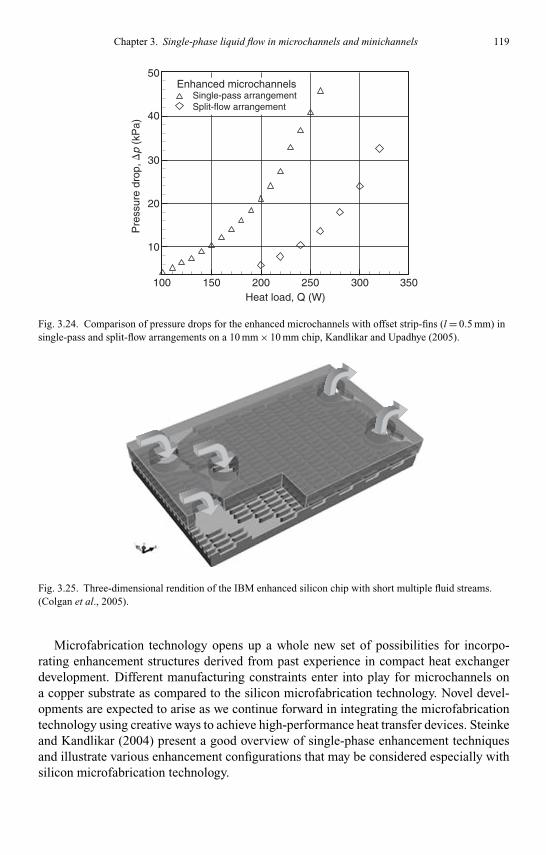
Kandlikar I044527-Ch03.tex 29/10/2005 9: 28 Page 119
Chapter 3. Single-phase liquid flow in microchannels and minichannels 119
40
30
Pre
ssur
e dr
op, �
p (k
Pa)
20
10
100 150 200 250 300Heat load, Q (W)
350
50Enhanced microchannels
Single-pass arrangementSplit-flow arrangement
Fig. 3.24. Comparison of pressure drops for the enhanced microchannels with offset strip-fins (l = 0.5 mm) insingle-pass and split-flow arrangements on a 10 mm × 10 mm chip, Kandlikar and Upadhye (2005).
Fig. 3.25. Three-dimensional rendition of the IBM enhanced silicon chip with short multiple fluid streams.(Colgan et al., 2005).
Microfabrication technology opens up a whole new set of possibilities for incorpo-rating enhancement structures derived from past experience in compact heat exchangerdevelopment. Different manufacturing constraints enter into play for microchannels ona copper substrate as compared to the silicon microfabrication technology. Novel devel-opments are expected to arise as we continue forward in integrating the microfabricationtechnology using creative ways to achieve high-performance heat transfer devices. Steinkeand Kandlikar (2004) present a good overview of single-phase enhancement techniquesand illustrate various enhancement configurations that may be considered especially withsilicon microfabrication technology.

Kandlikar I044527-Ch03.tex 29/10/2005 9: 28 Page 120
120 Heat transfer and fluid flow in minichannels and microchannels
0.5 100.6 0.70.8 0.9 1 2 3 4 5 6 7 9
Re∗(Dh /L)
30
150
40
50
60
70
80
90
100
Continuous 60 �m pitch (2)Stag., 100 �m pitch, wide chan. and no gap (5)Stag., 100 �m pitch, wide chan. and 40 �m gap (3)Stag., 100 �m pitch, narrow chan. and no gap (2)Stag., 100 �m pitch, narrow chan. and 40 �m gap (3)Model, y � 6.3x � 32.3
f∗ app
Re
Fig. 3.26. Apparent friction factor comparison of a plain and five enhanced microchannel configurations,Colgan et al. (2005).
4 805 6 7 8 10 20 30 40 50 60 70Re Pr Dh/L
2.5
30
5
6789
10
20
4
3
Nu
Continuous 75 �m pitchContinuous 60 �m pitch (2)
Stag., 100 �m pitch, wide chan. and no gap (5)
Stag., 100 �m pitch, wide chan. and 40 �m gap (3)Stag., 100 �m pitch, narrow chan. and no gap (2)Stag., 100 �m pitch, narrow chan. and 40 �m gap (3)laminar flow, theory (aspect ratio � 3)Model, y � 2.97(x^0.50)
Fig. 3.27. Nusselt number comparison of a plain and five enhanced microchannel configurations, Colganet al. (2005).
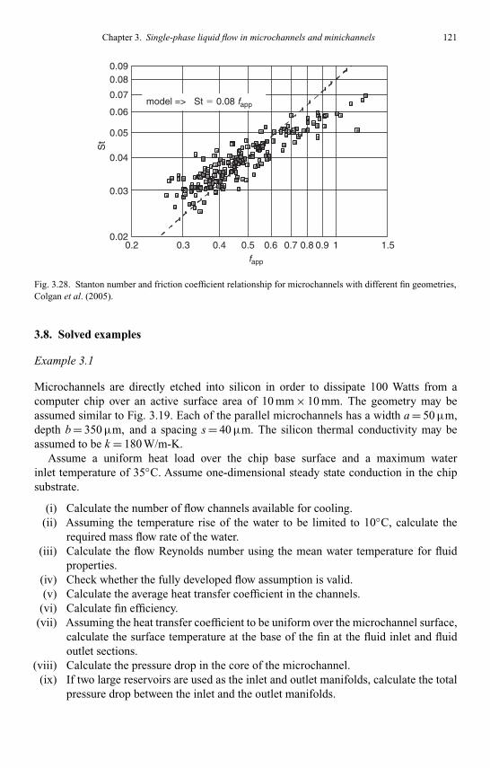
Kandlikar I044527-Ch03.tex 29/10/2005 9: 28 Page 121
Chapter 3. Single-phase liquid flow in microchannels and minichannels 121
0.2 0.3 0.4 0.5 0.6 0.7 0.8 0.9 1 1.5fapp
0.02
0.09
0.03
0.04
0.05
0.06
0.07
0.08
St
model => St � 0.08 fapp
Fig. 3.28. Stanton number and friction coefficient relationship for microchannels with different fin geometries,Colgan et al. (2005).
3.8. Solved examples
Example 3.1
Microchannels are directly etched into silicon in order to dissipate 100 Watts from acomputer chip over an active surface area of 10 mm × 10 mm. The geometry may beassumed similar to Fig. 3.19. Each of the parallel microchannels has a width a = 50 µm,depth b = 350 µm, and a spacing s = 40 µm. The silicon thermal conductivity may beassumed to be k = 180 W/m-K.
Assume a uniform heat load over the chip base surface and a maximum waterinlet temperature of 35◦C. Assume one-dimensional steady state conduction in the chipsubstrate.
(i) Calculate the number of flow channels available for cooling.(ii) Assuming the temperature rise of the water to be limited to 10◦C, calculate the
required mass flow rate of the water.(iii) Calculate the flow Reynolds number using the mean water temperature for fluid
properties.(iv) Check whether the fully developed flow assumption is valid.(v) Calculate the average heat transfer coefficient in the channels.
(vi) Calculate fin efficiency.(vii) Assuming the heat transfer coefficient to be uniform over the microchannel surface,
calculate the surface temperature at the base of the fin at the fluid inlet and fluidoutlet sections.
(viii) Calculate the pressure drop in the core of the microchannel.(ix) If two large reservoirs are used as the inlet and outlet manifolds, calculate the total
pressure drop between the inlet and the outlet manifolds.

Kandlikar I044527-Ch03.tex 29/10/2005 9: 28 Page 122
122 Heat transfer and fluid flow in minichannels and microchannels
SolutionProperties: Water at 40◦C (Incropera and DeWitt (2002))ρ= 991.8 kg/m3;µ= 655 × 10−6 N-s/m2; cp = 4179 J/kg-K; k = 0.632 W/m-K; Pr = 4.33
(i) Number of flow channels (Answer: 111 channels)Assumptions(1) The first and the last channels are half the channel width from the chip edge.
The remaining width left for channels is: 10 mm – 50 µm = 0.00995 m.The pitch is: 50 µm + 40 µm = 90 µm = 90 × 10−6 m.Assumption 1 requires that the pitch repeat up to the last channel, but not include the last
channel.Therefore, the number of channels is found by: (0.00995 m – 50 × 10−6 m)/(90 × 10−6 m) =
110 channels.But recall that that the above calculation was for a repeating pitch up to but not including
the last channel so the number of channels available for cooling is n = 111.
(ii) Required flow rate of water (Answer: 0.00239 kg/s or 143.6 ml/min, total)The inlet water temperature is given as 35◦C, and the stated assumption is that the watertemperature rise is limited to 10◦C.The mass flow rate can be calculated using the propertiesof water at the average temperature of 40◦C by using the equation q = mcpT where q isthe power dissipated from the chip, cp is the specific heat of water at constant pressure andT is the temperature change of the water. The total mass flow rate is
mt = q
cpT= 100 W/(4179 J/kg-K)(10 K) = 0.00239 kg/s = 143.6 ml/min,
and the mass flow rate in one channel is given by
mc = q
ncpT= 21.6 × 10⁻⁶ kg/s = 1.3 ml/min
(iii) Flow Reynolds number (Answer: Re = 164.7)The flow Reynolds number using the mean water temperature (40◦C) for fluid propertiescan be found using the hydraulic diameter Dh given by Eq. (3.7)
Dh = 2ab
(a + b)= 2(50 × 10−6 m)(350 × 10−6 m)/(50 × 10−6 m + 350 × 10−6 m)
= 87.5 × 10⁻⁶ m
in the Reynolds number equation given by
Re = ρumDh
µ= ρumAcDh
Acµ= mcDh
Acµ
= (21.6 × 10⁻⁶ kg/s)(87.5 × 10−6 m)
(17.5 × 10⁻⁹ m2)(655 × 10−6 N-s/m2)= 164.7
This low Reynolds number clearly indicates laminar flow regime.

Kandlikar I044527-Ch03.tex 29/10/2005 9: 28 Page 123
Chapter 3. Single-phase liquid flow in microchannels and minichannels 123
(iv) Fully developed assumption (Answer: fully developed assumption is valid –hydrodynamic entrance length = 0.72 mm and thermal entrance length = 6.25 mm)The fully developed flow assumption is valid if the thermal and hydrodynamic entrancelengths are less than the channel length. For laminar flow, the hydrodynamic entrancelength is given by Eq. (3.11) as
Lh = 0.05 Re Dh = 0.05(164.7)(87.5 × 10⁻⁶ m) = 720 × 10−6 m= 0.72 mm,
and the thermal entrance length is given by Eq. (3.42) as
Lt = 0.1Re Pr Dh = 0.1(164.7)(4.33)(87.5 × 10⁻⁶ m) = 6.24 × 10⁻³ m= 6.24 mm
Since the thermal and hydrodynamic entrance lengths are less than the channel length, thefully developed flow assumption is valid.
(v) Average heat transfer coefficient (Answer: 47.4 × 10³ W/m2-K)Assumptions(1) Constant heat flux boundary condition.(2) Three-sided heating condition.
The Nusselt number using the thermal conductivity of water at the average temperature(40◦C) is given by Nu = h Dh/k . A value for the fully developed Nusselt number can beobtained from Table 3.3 using the aspect ratio of the channel αc = a/b = 1/7. By linearinterpolation, the Nusselt number is Nufd,3 = 6.567.
The average heat transfer coefficient is
h = kNu
Dh= (0.632 W/m-K)(6.567)/87.5 × 10−6 m = 47.4 × 10³W/m2-K
(vi) Fin efficiency (Answer: 67%)Assumptions(1) Adiabatic tip condition.
For an adiabatic tip, the fin efficiency equation is given by ηf = tanh(mb)/mb where b isthe fin height
(350 × 10−6 m) and m is defined as m = (hP/kAc)1/2
In the above equation, k is thermal conductivity of the fin material (given as k =180 W/m-K), Ac is the cross-sectional area of the fin L × s = (0.01 m)(40 × 10−6 m), andP is the perimeter of the fin which can be defined as 2L since the width of the fin is muchsmaller than its length. The term mb can be written as
mb =(
h2L
ksL
)1/2
b =(
2h
ks
)1/2
b
=(
2(47.4 × 10³ W/m2-K)
(180 W/m-K)(40 × 10−6 m)
)1/2
(350 × 10−6 m) = 1.270

Kandlikar I044527-Ch03.tex 29/10/2005 9: 28 Page 124
124 Heat transfer and fluid flow in minichannels and microchannels
Therefore, the fin efficiency can be calculated as ηf = tanh(1.270)/1.270 = 0.672 = 67%.
(vii) Inlet and outlet surface temperatures at the base of the fin (Answer:T s,i = 36.3◦Cand T s,o = 48.6◦C)Assumptions(1) The heat flux is constant over the chip surface.
The surface heat flux considering the fin efficiency is given by
q′′ = q/(2bηf + a)nL
= 100 W[2(350 × 10−6 m)(0.672) + 50 × 10−6 m
](111)(0.01 m)
= 173 × 103 W/m2
The relationship between heat flux, heat transfer and temperature difference is given byq′′ = h(Ts − Tf ) where the subscripts s and f refer to the surface and fluid, respectively. Thelocal heat transfer coefficients at the inlet and outlet of the microchannels are needed inorder to compute the surface temperatures. Since the flow is developing at the entrance ofthe microchannel, Tables 3.3 and 3.4 are used with the channel aspect ratio and x* for theinlet, where x* is defined by Eq. (3.44). The entrance of the channel is assumed to beginat x = 0.1 mm from the edge of the chip so x* is
x∗in = 0.1 × 10⁻³ m
(87.5 × 10⁻⁶ m)(164.7)(4.33)= 1.603 × 10⁻³
Using linear interpolation in Table 3.3, the fully developed Nusselt numbers for three-sided and four-sided heating are found to be 6.567 and 6.273, respectively. The thermalentry region Nusselt number for four-sided heating is found using Table 3.4 to be 18.42for the inlet. Equation (3.45) is used to obtain the local Nusselt number at the entrance as
Nux,3(x∗,αc) = 18.426.567
6.273= 19.28
Alternatively, equations given in Appendix A may be used for interpolating values fromTables 3.2 to 3.4.
Using the thermal conductivity of water at the given inlet temperature (35◦C), the localheat transfer coefficient at the inlet is found to be
h = kNu
Dh= (0.625 W/m-K)(19.28)/87.5 × 10−6 m = 137.7 × 10³ W/m2-K
Since the flow is fully developed at the outlet, the three-sided Nusselt number fromTable 3.3is used with the thermal conductivity of water at the outlet temperature (45◦C). The localheat transfer coefficient at the exit is found to be
h = kNu
Dh= (0.638 W/m-K)(6.567)/87.5 × 10−6 m = 47.9 × 10³ W/m2-K

Kandlikar I044527-Ch03.tex 29/10/2005 9: 28 Page 125
Chapter 3. Single-phase liquid flow in microchannels and minichannels 125
Using the value of the heat flux obtained above, the local heat transfer coefficients, andthe given inlet and outlet water temperatures, the surface temperatures at the base of thefin at the fluid inlet and outlet are
Ts = q′′
h+ Tf => Ts,i = 36.3◦C and Ts,o = 48.6◦C
(viii) Pressure drop in microchannel core (Answer: 43.6 kPa)Assumptions
(1) The core of the microchannel includes pressure drop due to only frictional losses in thefully developed region and the loss due to the developing region.
Since the flow is fully developed at the exit, the pressure drop is defined by
p = 2( f Re)µumL
D2h
+ K(∞)ρu2
m
2
where K(∞) is the Hagenbach factor, which is defined by Eq. (3.18) as
K(∞) = 0.6796 + 1.2197αc + 3.3089α2c − 9.5921α3
c + 8.9089α4c − 2.9959α5
c
= 0.8969
The f Re term is given by Eq. (3.10) as
f Re = 24(1 − 1.3553αc + 1.9467α2c − 1.7012α3
c + 0.9564α4c − 0.2537α5
c)
= 20.2
The pressure drop in the core of the microchannel is given by Eq. (3.14) as
p = 2(20.2)(655 × 10−6 N-s/m2)(1.24 m/s)(0.01 m)
(87.5 × 10⁻⁶m)2
+ (0.8969)(991.8 kg/m3)(1.24 m/s)2
2= 43.6 kPa
(ix) Total pressure drop (Answer: 45.0 kPa)Assumptions(1) Reservoirs are large so the Area of the reservoir >> the Area of microchannel.
The total pressure drop between the inlet an outlet manifolds would include the pressuredrop calculated above (43.6 kPa) plus the minor losses at the entrance and exit.
The minor loss is defined by p = K(ρu2m/2) where K is a loss coefficient related to
area changes at the entrance or exit. Taking the area ratio as zero, based on Assumption 1,for a laminar flow regime, the contraction and expansion loss coefficients Kc and Ke canbe obtained from Fig. 3.5(b) as Kc = 0.8 and Ke = 1.0.
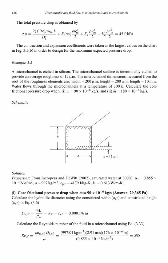
Kandlikar I044527-Ch03.tex 29/10/2005 9: 28 Page 126
126 Heat transfer and fluid flow in minichannels and microchannels
The total pressure drop is obtained by
p = 2( f Re)µum L
D2h
+ K(∞)ρu2
m
2+ Kc
ρu2m
2+ Ke
ρu2m
2= 45.0 kPa
The contraction and expansion coefficients were taken as the largest values on the chartin Fig. 3.5(b) in order to design for the maximum expected pressure drop.
Example 3.2
A microchannel is etched in silicon. The microchannel surface is intentionally etched toprovide an average roughness of 12 µm. The microchannel dimensions measured from theroot of the roughness elements are: width – 200 µm, height – 200 µm, length – 10 mm.Water flows through the microchannels at a temperature of 300 K. Calculate the corefrictional pressure drop when, (i) m = 90 × 10−6 kg/s, and (ii) m = 180 × 10−6 kg/s.
Schematic
b
e = 12 �ma
SolutionProperties: From Incropera and DeWitt (2002), saturated water at 300 K: µf = 0.855 ×10⁻³ N-s/m2, ρ= 997 kg/m3, cp,f = 4179 J/kg-K, kf = 0.613 W/m-K.
(i) Core frictional pressure drop when m = 90 × 10−6 kg/s (Answer: 29,365 Pa)Calculate the hydraulic diameter using the constricted width (acf ) and constricted height(bcf ) in Eq. (3.6)
Dh,cf = 4Ac
Pw= acf = bcf = 0.000176 m
Calculate the Reynolds number of the fluid in a microchannel using Eq. (3.33)
Recf = ρum,cf Dh,cf
µ= (997.01 kg/m3)(2.91 m/s)(176 × 10−6 m)
(0.855 × 10⁻³ Ns/m2)= 598

Kandlikar I044527-Ch03.tex 29/10/2005 9: 28 Page 127
Chapter 3. Single-phase liquid flow in microchannels and minichannels 127
For fully developed laminar flow, the hydrodynamic entry length may be obtained usingEq. (3.11)
Lh,cf = 0.05 Recf Dh,cf = 0.05(598)(0.176 mm) = 5.26 mm
Since L>Lh,cf , the fully developed flow assumption is valid.The f Re term can be obtained using Eq. (3.10)
f Re = 24(1 − 1.3553αc + 1.9467α2c − 1.7012α3
c + 0.9564α4c − 0.2537α5
c)
= 14.23
The core frictional pressure drop can be calculated using Eq. (3.14)
p = 2( f Re)µm,cf L
D2h,cf
+ K(∞)ρu2
m,cf
where K(∞) is given by Eq. (3.18)
K(∞) = (0.6796 + 1.2197αc + 3.3089α2c − 9.5921α3
c + 8.9089α4c − 2.9959α5
c)
= 1.53
Hence
p = 2(14.23)(0.855 × 10⁻³ Ns/m2)(2.91 m/s)(0.01 m)
(176 × 10−6 m)2
+ (1.53)(997.01 kg/m3)(2.91 m/s)2
2= 29,365 Pa
(ii) Core frictional pressure drop when m = 180 × 10−6 kg/s (Answer: 68,694 Pa)Calculate the Reynolds number of the fluid in a microchannel using Eq. (3.33)
Recf = ρum,cf Dh,cf
µ= (997.01 kg/m3)(5.83 m/s)(176 × 10−6 m)
(0.855 × 10⁻³ Ns/m2)= 1200
For fully developed laminar flow, the hydrodynamic entry length may be obtained usingEq. (3.11)
Lh,cf = 0.05 Recf Dh,cf = 0.05(1200)(0.176 mm) = 10.5 mm
Since L<Lh,cf , the fully developed flow assumption is not valid.Calculate the core frictional pressure drop with the developing laminar flow assumption.
The apparent friction factor can be obtained from Table 3.2 using x+ calculated fromEq. 3.16
x+ = x/Dh
Recf= 0.01 m
(176 × 10−6 m)(1200)= 0.0475

Kandlikar I044527-Ch03.tex 29/10/2005 9: 28 Page 128
128 Heat transfer and fluid flow in minichannels and microchannels
From Table 3.2 fapp Re = 21.35 so the core frictional pressure drop can be calculated usingthe following equation
p = 2( fappRe)µm,cf L
D2h,cf
= 2(21.35)(0.855 × 10⁻³ Ns/m2)(5.83 m/s)(0.01 m)
(176 × 10−6 m)2 = 68,694 Pa
Comments(1) The total frictional pressure drop has to consider the minor losses because the actual
p is higher than the core frictional pressure drop.
Example 3.3
Consider a copper minichannel heat sink with an area of 30 mm × 30 mm, and relevantdimensions in Fig. 3.14 with a = 1 mm, b = 3 mm, and s = 1.5 mm. The heat dissipationis 100 W and the water inlet temperature is 30◦C. The maximum surface temperature inthe heat sink is limited to 80◦C. Calculate the water flow rate under these conditions.Also calculate the frictional pressure drop in the core. Assume a constant heat transfercoefficient corresponding to fully developed conditions and take the thermal conductivityof copper to be 400 W/m-K.
AssumptionsLaminar flow, constant heat flux equally distributed over the surface area, one-dimensionalsteady state conduction, and three-sided heated condition with an adiabatic tip for finefficiency
a = 1 mm = 10−3 m, b = 3 mm = 3 × 10⁻³ m, s = 1.5 mm = 1.5 × 10⁻³ m, w= L = 30 ×10−3 m, Tf ,i = 30◦C, Ts,o = 80◦C, q =100 W, kCu = 400 W/m-K, Ac = a×b = 3 × 10⁻⁶ m2,αc = a/b = 1/3
b
a s
SolutionEquation 3.7 gives the hydraulic diameter,
Dh = 2ab
(a + b)= 2(10−3)(3 × 10⁻³)
(10−3 + 3 × 10⁻³)= 1.5 × 10⁻³ m

Kandlikar I044527-Ch03.tex 29/10/2005 9: 28 Page 129
Chapter 3. Single-phase liquid flow in microchannels and minichannels 129
The Nusselt number can be obtained using Table 3.3 for a three-sided heated channel.Through interpolation this gives,
Nu = Nufd,3 = 5.224
For calculating water properties, let’s assume the water exit temperature is equal to themaximum surface temperature of the heat sink. Then, the average water temperature is,
Tavg = (30◦C + 80◦C)/2 = 55◦C
Properties of water at 55◦C (from Incropera and DeWitt, 2002):
ρ = 985 kg/m3, cp = 4.183 kJ/kg-K, µ = 505 × 10−6 kg/m-s,
k = 648 × 10−3 W/m-K
The average heat transfer coefficient is calculated using the Nusselt number which isrearranged to give,
h = kNu
Dh= (0.648)(5.224)
(1.5 × 10⁻³)= 2.26 × 10³ W/m2-K
By relating the conductive and convective heat transfer for a constant heat flux, theaverage temperature difference between the surface and the fluid is given as
T = q
h(2bηf + a)nL
The number of channels is, n = overall width
channel + fin= w
a + s= 0.030
0.001 + 0.0015= 12
The fin efficiency is, ηf = tanh(mb)
mb
mb =√
2h
kCusb =
√2(2.26 × 10³)
(400)(1.5 × 10−3)× (3 × 10−3) = 0.260
ηf = tanh(0.260)
(0.260)= 0.978
T(x)
x
T s,o
T f,o
Tf,i
Ts,i
hq �
∆T �
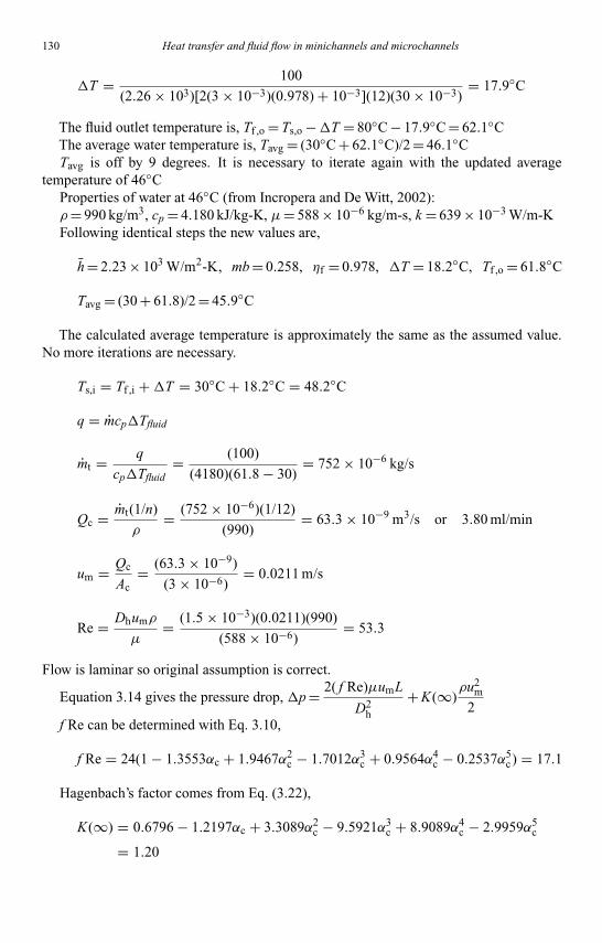
Kandlikar I044527-Ch03.tex 29/10/2005 9: 28 Page 130
130 Heat transfer and fluid flow in minichannels and microchannels
T = 100
(2.26 × 10³)[2(3 × 10⁻³)(0.978) + 10−3](12)(30 × 10−3)= 17.9◦C
The fluid outlet temperature is, Tf ,o = Ts,o −T = 80◦C − 17.9◦C = 62.1◦CThe average water temperature is, Tavg = (30◦C + 62.1◦C)/2 = 46.1◦CTavg is off by 9 degrees. It is necessary to iterate again with the updated average
temperature of 46◦CProperties of water at 46◦C (from Incropera and De Witt, 2002):ρ= 990 kg/m3, cp = 4.180 kJ/kg-K, µ= 588 × 10−6 kg/m-s, k = 639 × 10−3 W/m-KFollowing identical steps the new values are,
h = 2.23 × 10³ W/m2-K, mb = 0.258, ηf = 0.978, T = 18.2◦C, Tf ,o = 61.8◦C
Tavg = (30 + 61.8)/2 = 45.9◦C
The calculated average temperature is approximately the same as the assumed value.No more iterations are necessary.
Ts,i = Tf ,i +T = 30◦C + 18.2◦C = 48.2◦C
q = mcpTfluid
mt = q
cpTfluid= (100)
(4180)(61.8 − 30)= 752 × 10−6 kg/s
Qc = mt(1/n)
ρ= (752 × 10−6)(1/12)
(990)= 63.3 × 10⁻⁹ m3/s or 3.80 ml/min
um = Qc
Ac= (63.3 × 10⁻⁹)
(3 × 10⁻⁶)= 0.0211 m/s
Re = Dhumρ
µ= (1.5 × 10⁻³)(0.0211)(990)
(588 × 10−6)= 53.3
Flow is laminar so original assumption is correct.
Equation 3.14 gives the pressure drop, p = 2( f Re)µumL
D2h
+ K(∞)ρu2
m
2f Re can be determined with Eq. 3.10,
f Re = 24(1 − 1.3553αc + 1.9467α2c − 1.7012α3
c + 0.9564α4c − 0.2537α5
c) = 17.1
Hagenbach’s factor comes from Eq. (3.22),
K(∞) = 0.6796 − 1.2197αc + 3.3089α2c − 9.5921α3
c + 8.9089α4c − 2.9959α5
c
= 1.20
Kandlikar I044527-Ch03.tex 29/10/2005 9: 28 Page 131
Chapter 3. Single-phase liquid flow in microchannels and minichannels 131
The pressure drop in the core is therefore,
p = 2(17.1)(588 × 10−6)(0.0211)(30 × 10−3)
(1.5 × 10⁻³)2 + (1.20)(990)(0.0211)2
2= 5.92 Pa
We need to calculate the hydrodynamic and thermal entrance lengths to justify fullydeveloped conditions.
Using Eq. (3.11) we have, Lh = 0.05 Dh Re = 0.05(1.5 × 10⁻³)(53.3) = 0.00400 m =4.00 mm
Similarly Eq. (3.42) gives, Lt = 0.05 Dh Re Pr = 0.05(1.5 × 10⁻³)(53.3)(3.85) =0.0154 m = 15.4 mm
This validates the fully developed assumption as given in the problem statement.
CommentsIf the heat dissipation is increased to 200 W the flow rate will be 18.4 ml/min. This increasesthe pressure drop to 38.8 Pa. This illustrates the performance hit for increased heat dis-sipation and the need to develop microchannel cooling under turbulent conditions wherethe heat transfer coefficient will be larger. For turbulent flow more heat can be dissipatedwith minimal performance loss in pressure drop.
3.9. Practice problems
Problem 3.1 Solve Example 1 with the substrate as copper, with a thermal conductivityof 380 W/m-K.
Problem 3.2 For Example 3.1, plot the outlet surface temperature and pressure drop asa function of the channel depth b over a range of 200 to 600 µm.
Problem 3.3 For Example 3.1, plot the outlet surface temperature and pressure drop asa function of the channel width a over a range of 50 to 200 µm.
Problem 3.4 Solve Example 3.1 with a split flow arrangement. Neglect the areareduction caused by the central manifold.
Problem 3.5 Solve Example 3.1 with copper substrate and a split flow arrangement.Assume the channel width to be 100 µm and a depth of 800 µm. Neglect the area reductioncaused by the central manifold.
Problem 3.6 For Example 3.3 with copper, plot the outlet surface temperature and thepressure drop as a function of the channel depth over a range of 200 to 2000 µm.
Problem 3.7 In Example 3.3, redesign the heat sink if the design heat load increases to500 W. You may have to rework the channel geometry and flow arrangements.
Problem 3.8 Design a microchannel heat exchanger to dissipate 800 Watts from a copperheat sink of 20 mm × 20 mm heated surface area. The inlet water temperature is 40◦C, and
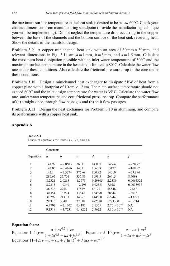
Kandlikar I044527-Ch03.tex 29/10/2005 9: 28 Page 132
132 Heat transfer and fluid flow in minichannels and microchannels
the maximum surface temperature in the heat sink is desired to be below 60◦C. Check yourchannel dimensions from manufacturing standpoint (provide the manufacturing techniqueyou will be implementing). Do not neglect the temperature drop occurring in the copperbetween the base of the channels and the bottom surface of the heat sink receiving heat.Show the details of the manifold design.
Problem 3.9 A copper minichannel heat sink with an area of 30 mm × 30 mm, andrelevant dimensions in Fig. 3.14 are a = 1 mm, b = 3 mm, and s = 1.5 mm. Calculatethe maximum heat dissipation possible with an inlet water temperature of 30◦C and themaximum surface temperature in the heat sink is limited to 80◦C. Calculate the water flowrate under these conditions. Also calculate the frictional pressure drop in the core underthese conditions.
Problem 3.10 Design a minichannel heat exchanger to dissipate 5 kW of heat from acopper plate with a footprint of 10 cm × 12 cm. The plate surface temperature should notexceed 60◦C and the inlet design temperature for water is 35◦C. Calculate the water flowrate, outlet water temperature, and core frictional pressure drop. Compare the performanceof (a) straight once-through flow passages and (b) split flow passages.
Problem 3.11 Design the heat exchanger for Problem 3.10 in aluminum, and compareits performance with a copper heat sink.
Appendix A
Table A.1Curve-fit equations for Tables 3.2, 3.3, and 3.4
Constants
Equations a b c d e f
1 141.97 −7.0603 2603 1431.7 14364 −220.772 142.05 −5.4166 1481 1067.8 13177 −108.523 142.1 −7.3374 376.69 800.92 14010 −33.8944 286.65 25.701 337.81 1091.5 26415 8.40985 8.2321 2.0263 1.2771 0.29805 2.2389 0.00653226 8.2313 1.9349 −2.295 0.92381 7.928 0.00339377 36.736 2254 17559 66172 555480 1212.68 30.354 1875.4 13842 154970 783440 −8015.19 31.297 2131.3 14867 144550 622440 −13297
10 28.315 3049 27038 472520 1783300 −3571411 6.7702 −3.1702 0.4187 2.1555 2.76 × 10⁻⁶ NA12 9.1319 −3.7531 0.48222 2.5622 5.16 × 10⁻⁶ NA
Equation form:
Equations 1–4: y = a + cx0.5 + ex
1 + bx0.5 + dx + fx1.5 ; Equations 5–10: y = a + cx + ex2
1 + bx + dx2 + fx3
Equations 11–12: y = a + bx + c(ln x)2 + d ln x + ex−1.5

Kandlikar I044527-Ch03.tex 29/10/2005 9: 28 Page 133
Chapter 3. Single-phase liquid flow in microchannels and minichannels 133
Equation variablesLaminar flow friction factor in entrance region of rectangular ducts, Table 3.2:
y-variable – friction factorx-variable – Equation 1: αc = 1.0
Equation 2: αc = 0.5Equation 3: αc = 0.2Equation 4: 0.1 =αc = 10
Fully developed Nusselt number for three-side heating, Table 3.3:
y-variable – Nusselt number for three-sided heatingx-variable – Equation 5: αc
Fully developed Nusselt number for four-side heating, Table 3.3:
y-variable – Nusselt number for four-sided heatingx-variable – Equation 6: αc
Thermal entry region Nusselt numbers for four-sided heating, Table 3.4:
y-variable – Nusselt number for four-sided heating in the entry regionx-variable – Equation 7: αc = 0.1
Equation 8: αc = 0.25Equation 9: αc = 0.333Equation 10: αc = 0.5Equation 11: αc = 1.0Equation 12: αc = 10
References
Adams, T. M., Abdel-Khalik, S. I., Jeter, M., and Qureshi, Z. H., An experimental investigation ofsingle-phase forced convection in microchannels, Int. J. Heat. Mass Trans., 41(6–7), 851–857,1997.
ASME Standard B46.1-2002, Surface Texture (Surface Roughness, Waviness, and Lay), The Amer-ican Society of Mechanical Engineers, An American National Standard, (ASME B46.1-2002),1–98.
Baviere, R. and Ayela, F., First local measurement in microchannels with integrated micromachinedstrain gauges, Paper No. ICMM2004-2406, Second International Conference on Microchannelsand Minichannels, Rochester, NY USA, June 17–19, 221–228, 2004.
Baviere, R., Ayela, F., Le Person, S., and Favre-Marinet, M., 2004, An experimental study ofwater flow in smooth and rough rectangular microchannels, Paper No. ICMM2004-2338, SecondInternational Conference on Microchannels and Minichannels, Rochester, NY USA, June 17–19,221–228, 2004.
Bergles, A. E., Lienhard, J. H., V, Kendall, G. E., and Griffith, P., Boiling and condensation in smalldiameter channels, Heat Transfer Eng., 24, 18–40, 2003.
Bucci, A., Celata, G. P., Cumo, M., Serra, E., and Zummo, G., Water single-phase fluidflow and heat transfer in capillary tubes, Paper No. ICMM2004-2406, Second InternationalConference on Microchannels and Minichannels, Rochester, NY USA, June 17–19, 221–228,

Kandlikar I044527-Ch03.tex 29/10/2005 9: 28 Page 134
134 Heat transfer and fluid flow in minichannels and microchannels
2004. International Conference on Microchannels and Minichannels. Paper # 1037, ASME,319–326.
Celata, G. P., Cumo, M., Guglielmi, M., and Zummo, G., Experimental investigation of hydraulic andsingle phase heat transfer in 0.130 mm capillary tube, Microscale Thermophys. Eng., 6, 85–97,2002.
Chen, R.Y., Flow in the entrance region at low Reynolds numbers, J. Fluid. Eng., 95, 153–158, 1972.Colgan, E. G., Furman, B., Gaynes, M., Graham, W., LaBianca, N., Magerlein, J. H., Polastre, R. J.,
Rothwell, M. B., Bezama, R. J., Choudhary, R., Martson, K., Toy, H., Wakil, J., Zitz, J., andSchmidt, R., A practical implementation of silicon microchannel coolers for high power chips,Invited Paper presented at IEEE-Semi-Therm 21, San Jose, March 15–17, 2005.
Curr, R. M., Sharma, D., and Tatchell, D. G., Numerical predictions of some three-dimensionalboundary layers in ducts, Comput. Method. Appl. Mech. Eng., 1, 143–158, 1972.
Darcy, H., Recherches experimentales relatives au movement de L’Eau dans lesTuyaux, Paris, France:Mallet-Bachelier, 1857.
Fanning, J. T., A practical treatise on hydraulic and water supply engineering, New York: VanNostrand, 1886 (revised edition of 1877).
Gad-el-Hak, M., The fluid mechanics of microdevices, J. Fluid. Eng., 121, 7–33, 1999.Gamrat, G., Favre-Marinet, M., and Asendrych, D., Numerical modeling of heat transfer in rectan-
gular microchannels, Paper No. ICMM2004-2336, ASME, Second International Conference onMicrochannels and Minichannels, June 16–18, Rochester, NY, 205–212, 2004.
Garimella, S. V., and Singhal, V., Single-phase flow and heat transport and pumping considerationsin microchannel heat sinks, Heat Trans. Eng., 25(1), 15–25, 2004.
Gnielinski, V., New equations for heat and mass transfer in turbulent pipe and channel flow, Int.Chem. Eng., 16, 359–368, 1976.
Harpole, G. and Eninger, J. E., Micro-channel heat exchanger optimization, Proceedings – IEEESemiconductor Thermal and Temperature Measurement Symposium, 59–63, Feb, 1991.
Hartnett, J. P., Koh, J. C. Y., and McComas, S. T., A comparison of predicted and measured frictionfactors for turbulent flow through rectangular ducts, J. Heat Trans., 84, 82–88, 1962.
Hornbeck, R. W., Laminar flow in the entrance region of a pipe, Appl. Sci. Res., 13, 224–232, 1964.Jones Jr., O. C., An improvement in the calculation of turbulent friction in rectangular ducts, J. Fluid.
Eng., 98, 173–181, 1976.Judy, J., Maynes, D., and Webb, B. W., Characterization of frictional pressure drop for liquid flows
through microchannels, Int. J. Heat Mass Trans, 45, 3477–3489, 2002.Kakac, S., Shah, R. K., and Aung, W., Handbook of Single-Phase Convective Heat Transfer, New
York: John Wiley and Sons, Inc., 1987.Kandlikar, S. G. High heat flux removal with microchannels – A roadmap of challenges and
opportunities, Heat Trans. Eng., 26(8), 2005.Kandlikar, S. G. and Grande, W. J., Evaluation of single-phase flow in microchannels for high
flux chip cooling – thermohydraulic performance enhancement and fabrication technology, HeatTrans. Eng., 25(8), 5–16, 2004.
Kandlikar, S. G., Joshi, S., and Tian, S., Effect of surface roughness on heat transfer and fluid flowcharacteristics at low Reynolds numbers in small diameter tubes, Heat Trans. Eng., 24(3), 4–16,2003.
Kandlikar, S. G. and Upadhye, H. R., Extending the heat flux limit with enhanced microchannels indirect single-phase cooling of computer chips, Invited Paper presented at IEEE-Semi-Therm 21,San Jose, March 15–17, 2005.
Kandlikar, S.G., Schmitt, D., Carrano, A. L., and Taylor, J. B., Characterization of surface rough-ness effects on pressure drop in single-phase flow in minichannels, Phys. Fluid., 17, 2005(accepted).

Kandlikar I044527-Ch03.tex 29/10/2005 9: 28 Page 135
Chapter 3. Single-phase liquid flow in microchannels and minichannels 135
Kays, W. M. and London, A. L., Compact Heat Exchangers, New York, NY: McGraw-Hill, 1984.Kishimoto, T. and Sasaki, S., Cooling characteristics of diamond-shaped interrupted cooling fins for
high power LSI devices, Electron. Letter., 23(9), 456–457, 1987.Knight, R. W., Hall, D. J., Goodling, J. S., and Jaeger, R. C., Heat sink optimization with application
to microchannels, IEEE Transactions on Components, Hybrids, and Manufacturing Technology,15(5), 832–842, 1992.
Koo, J. and Kleinstreuer, C., Analyses of liquid flow in micro-conduits, Paper No. ICMM2004-2334,ASME, Second International Conference on Microchannels and Minichannels, Rochester, NY,June 17–19, 191–198, 2004.
Li, Z. X., Du, D. X., and Guo, Z. Y., Experimental study on flow characteristics of liquid incircular microtubes, Proceeding of the International Conference on Heat Transfer and TransportPhenomena in Microscale, Banff, Canada, October 15–20, 162–167, 2000.
Mises, R. v., Elemente der Technischen Hydrodynamik, Leipzig, B. G. Teubner, 1914.Moody, L. F., Friction factors for pipe flow, ASME Transactions, 66, 671–683, 1944.Niklas, M. and Favre-Marinet, M., Pressure losses in a network of triangular minichannels, ASME,
Paper No. ICMM2003-1039, First International Conference on Microchannels and Minichannels,April 24–25, 335–350, 2003.
Nikuradse, J., Strommungsgesetze in Rauen Rohren, VDI-Forschungsheft 361, Belige zu Forschungauf dem Gebiete des Ingenieurwesens Ausage B Band 4, July/August 1933. English TranslationLaws of flow in rough pipes, NACA Tech. Mem. 1292, 1937.
Phillips, R. J., Forced convection, liquid cooled, microchannel heat sinks, MS Thesis, Departmentof Mechanical Engineering, Massachusetts Institute of Technology, Cambridge, MA, 1987.
Phillips, R. J., Microchannel heat sinks, Advances in Thermal Modeling of Electronic Componentsand Systems, New York, NY: Hemisphere Publishing Corporation, 1990, Chapter 3.
Ryu, J. H., Choi, D. H., and Kim, S. J., Numerical optimization of the thermal performance of amicrochannel heat sink, Int. J. Heat Mass Trans., 45, 2823–2827, 2002.
Schmitt, D. J. and Kandlikar, S. G., Effects of repeating microstructures on pressure drop in rect-angular minichannels, Paper No. ICMM2005-75111, ASME, Third International Conference onMicrochannels and Minichannels, Toronto, Canada, June 13–15, 2005.
Shah, R. K. and London, A. L., Laminar Flow Forced Convection in Ducts, Supplement 1 toAdvancesin Heat Transfer, New York: Academic Press, 1978.
Shen, P., Aliabadi, S. K., and Abedi, J., A review of single-phase liquid flow and heat trans-fer in microchannels, Paper ICMM2004-2337, ASME, Second International Conference onMicrochannels and Minichannels, June 17–19, 213–220, 2004.
Steinke, M. E., Characterization of single-phase fluid flow and heat transfer in plain and enhanced sil-icon microchannels, PhD Thesis, Rochester, NY: Microsystems Engineering, Rochester Instituteof Technology, 2005.
Steinke, M. E. and Kandlikar, S. G., Single-phase enhancement techniques in microchannel flows,Paper No. ICMM2004-2328, ASME, Second International Conference on Microchannels andMinichannels, Rochester, NY, June 17–19, 2004.
Steinke, M. E. and Kandlikar, S. G., Single-phase liquid friction factors in microchannels, Paper No.ICMM2005-75112, ASME, Third International Conference on Microchannels and Minichannels,Toronto, Canada, June 13–15, 2005a.
Steinke, M. E. and Kandlikar, S. G., Review of single-phase liquid heat transfer in microchannels,Paper No. ICMM2005-75114, ASME, Third International Conference on Microchannels andMinichannels, Toronto, Canada, June 13–15, 2005b.
Steinke, M. E. and Kandlikar, S. G., Development of an experimental facility for investigating single-phase liquid flow in microchannels, Paper No. ICMM2005-75070, ASME, Third InternationalConference on Microchannels and Minichannels, Toronto, Canada, June 13–15, 2005c.

Kandlikar I044527-Ch03.tex 29/10/2005 9: 28 Page 136
136 Heat transfer and fluid flow in minichannels and microchannels
Tu, X. and Hrnjak, P., Experimental investigation of single-phase flow and pressure dropthrough rectangular microchannels, ASME, ICMM2003-1028, First International Conferenceon Microchannels and Minichannels, April 24–25, 257–267, 2003.
Tuckerman, D. B. and Pease, R. F. W., High performance heat sink for VLSI, IEEE Electron Dev.Lett., EDL-2, (5), 126–129, 1981.
Tuckerman, D.B., Heat transfer microstructures for integrated circuits, PhD Thesis, Stanford, CA,Stanford University, 1984.
Webb, R. L., Eckert, E. R. G., and Goldstein, R. J., Heat transfer and friction in tubes with repeated-ribroughness, Int. J. Heat and Mass Trans., 14, 601–617, 1971.
Wibulswas, P., Laminar flow heat transfer in non-circular ducts, PhD Thesis, London, UK, LondonUniversity, 1966.
Xu, B., Ooi, K. T., Wong, N. T., and Choi, W. K., Experimental investigation of flow friction forliquid flow in microchannels, Int. Com. Heat Mass Trans., 27(8), 1165–1176, 2000.
Yu, D., Warrington, R., Barron, R., and Ameel, T., An experimental investigation of fluid flow andheat transfer in microtubes, Proceedings of the ASME/JSME Thermal Engineering Conference,1, ASME, 523–530, 1995.

Kandlikar I044527-Ch04.tex 28/10/2005 16: 47 Page 137
Chapter 4
SINGLE PHASE ELECTROKINETIC FLOW INMICROCHANNELS
Dongqing Li
Department of Mechanical Engineering, Vanderbilt University, Nashville, TN, USA
4.1. Introduction
It is important to understand electrokinetic-driven liquid flow in microchannels whendesigning and controlling lab-on-a-chip devices. Lab-on-a-chip devices are miniaturizedbio-medical or chemistry laboratories on a small glass or plastic chip. Generally, a lab-on-a-chip device has a network of microchannels, electrodes, sensors and electrical circuits.Electrodes are placed at strategic locations on the chip. Applying electrical fields alongmicrochannels controls the liquid flow and other operations in the chip. These labs on a chipcan duplicate the specialized functions as their room-sized counterparts, such as clinicaldiagnostics, DNA scanning and electrophoretic separation. The advantages of these labson a chip include dramatically reduced sample size, much shorter reaction and analysistime, high throughput, automation and portability.
The key microfluidic functions required in various lab-on-a-chip devices includepumping, mixing, thermal cycling, dispensing and separating. Most of these processesare electrokinetic processes. Basic understanding, modeling and controlling of these keymicrofluidic functions/processes are essential to systematic design and operational con-trol of the lab-on-a-chip systems. Because all solid–liquid (aqueous solutions) interfacescarry electrostatic charge, there is an electrical double layer (EDL) field in the regionclose to the solid–liquid interface on the liquid side. Such an EDL field is responsible forat least two basic electrokinetic phenomena: electroosmosis and electrophoresis. Briefly,electroosmosis is the liquid motion in a microchannel caused by the interaction betweenthe EDL at the liquid-channel wall interface with an electrical field applied tangentiallyto the wall. Electrophoresis is the motion of a charged particle relative to the surroundingliquid under an applied electrical field. Essentially all on-chip microfluidic processes arerealized by using these two phenomena. This chapter will review basics of the EDL field,
E-mail: [email protected]
137

Kandlikar I044527-Ch04.tex 28/10/2005 16: 47 Page 138
138 Heat transfer and fluid flow in minichannels and microchannels
and discuss some key on-chip microfluidic processes. A more comprehensive review ofthe electrokinetic-based microfluidic processes for lab-on-a-chip applications can be foundelsewhere (Li, 2004).
4.2. EDL field
It is well-known that most solid surfaces obtain a surface electric charge when they arebrought into contact with a polar medium (e.g. aqueous solutions). This may be due toionization, ion adsorption or ion dissolution. If the liquid contains a certain amount of ions(for instance, an electrolyte solution or a liquid with impurities), the electrostatic chargeson the solid surface will attract the counterions in the liquid. The rearrangement of thecharges on the solid surface and the balancing charges in the liquid is called the EDL(Hunter, 1981; Lyklema, 1995). Immediately next to the solid surface, there is a layer ofions that are strongly attracted to the solid surface and are immobile. This layer is calledthe compact layer, normally about several Angstroms thick. Because of the electrostaticattraction, the counterions concentration near the solid surface is higher than that in the bulkliquid far away from the solid surface. The coions concentration near the surface, however,is lower than that in the bulk liquid far away from the solid surface, due to the electricalrepulsion. So there is a net charge in the region close to the surface. From the compact layerto the uniform bulk liquid, the net charge density gradually reduces to zero. Ions in thisregion are affected less by the electrostatic interaction and are mobile. This region is calledthe diffuse layer of the EDL. The thickness of the diffuse layer is dependent on the bulkionic concentration and electrical properties of the liquid, usually ranging from severalnanometers for high ionic concentration solutions up to several microns for pure waterand pure organic liquids. The boundary between the compact layer and the diffuse layeris usually referred to as the shear plane. The electrical potential at the solid–liquid surfaceis difficult to measure directly. The electrical potential at the shear plane is called the zetapotential ζ and can be measured experimentally (Hunter, 1981; Lyklema, 1995). In practice,the zeta potential is used as an approximation to the potential at the solid–liquid interface.
The ion and electrical potential distributions in the EDL can be determined by solvingthe Poisson–Boltzmann equation (Hunter, 1981; Lyklema, 1995). According to the theoryof electrostatics, the relationship between the electrical potentialψ and the local net chargedensity per unit volume ρe at any point in the solution is described by the Poisson equation:
∇2ψ = −ρe
ε(4.1)
where ε is the dielectric constant of the solution. Assuming the equilibrium Boltzmanndistribution equation is applicable, which implies uniform dielectric constant, the numberconcentration of the type-i ion is of the form
ni = nio exp(
− zieψ
kbT
)(4.2)
where nio and zi are the bulk ionic concentration and the valence of type-i ions, respectively,e is the charge of a proton, kb is the Boltzmann constant, and T is the absolute temperature.
Kandlikar I044527-Ch04.tex 28/10/2005 16: 47 Page 139
Chapter 4. Single phase electrokinetic flow in microchannels 139
For a symmetric electrolyte (z− = z+ = z) solution, the net volume charge density ρe isproportional to the concentration difference between symmetric cations and anions, via.:
ρe = ze(n+ − n−) = −2zeno sinh(
zeψ
kbT
)(4.3)
Substituting Eq. (4.3) into the Poisson equation leads to the well-known Poisson–Boltzmann equation:
∇2ψ = 2zeno
εsinh
(zeψ
kbT
)(4.4)
Solving the Poisson–Boltzmann equation with proper boundary conditions will deter-mine the local EDL potential field ψ and hence, via Eq. (4.3), the local net charge densitydistribution.
4.3. Electroosmotic flow in microchannels
Consider a microchannel filled with an aqueous solution. There is an EDL field near theinterface of the channel wall and the liquid. If an electric field is applied along the lengthof the channel, an electrical body force is exerted on the ions in the diffuse layer. In thediffuse layer of the EDL field, the net charge density, ρe is not zero. The net transport ofions is the excess counterions. If the solid surface is negatively charged, the counterionsare the positive ions. These excess counterions will move under the influence of the appliedelectrical field, pulling the liquid with them and resulting in electroosmotic flow. The liquidmovement is carried through to the rest of the liquid in the channel by viscous forces. Thiselectrokinetic process is called electroosmosis and was first introduced by Reuss in 1809(Reuss, 1809).
In most lab-on-a-chip applications, electroosmotic flow is preferred over the pressure-driven flow. One of the reasons is the plug-like velocity profile of electroosmotic flow.This means that fluid samples can be transported without dispersion caused by flow shear.Generally, pumping a liquid through a small microchannel requires applying very largepressure difference depending on the flow rate. This is often impossible because of thelimitations of the size and the mechanical strength of the microfluidic devices. Electroos-motic flow can generate the required flow rate even in very small microchannels withoutany applied pressure difference across the channel. Additionally, using electroosmotic flowto transport liquids in complicated microchannel networks does not require any externalmechanical pump or moving parts, it can be easily realized by controlling the electricalfields via electrodes. Although high voltages are often required in electroosmotic flow,the required electrical power is very small due to the very low current involved, and it isgenerally safe. However, the heat produced in electroosmotic flow often presents problemsto many applications where solutions of high electrolyte concentrations and long operationtime are required.
Most channels in modern microfluidic devices and micro-electro-mechanical systems(MEMS) are made by micromachining technologies. The cross-section of these channels

Kandlikar I044527-Ch04.tex 28/10/2005 16: 47 Page 140
140 Heat transfer and fluid flow in minichannels and microchannels
x
y
z L
2W
2H
Fig. 4.1. Geometry of microchannel. The shaded region indicates the computational domain.
is close to a rectangular shape. In such a situation, the EDL field is two-dimensionaland will affect the two-dimensional flow field in the rectangular microchannel. In order tocontrol electroosmotic pumping as a means of transporting liquids in microstructures, wemust understand the characteristics of electroosmotic flow in rectangular microchannels.In the following, we will review the modeling and the numerical simulation results ofelectroosmotic flow in rectangular microchannels (Arulanandam and Li, 2000a). The EDLfield, the flow field and the volumetric flow rate will be studied as functions of the zetapotential, the liquid properties, the channel geometry and the applied electrical field.
Consider a rectangular microchannel of width 2W , height 2H and length L, as illustratedin Fig. 4.1. Because of the symmetry in the potential and velocity fields, the solution domaincan be reduced to a quarter section of the channel (as shown by the shaded area in Fig. 4.1).
The 2D EDL field can be described by the Poisson–Boltzmann equation:
∂2ψ
∂y2 + ∂2ψ
∂z2 = 2n∞ze
εε0sinh
(− zeψ
kbT
)
Along the planes of symmetry, the following symmetry boundary conditions apply:
at y = 0∂ψ
∂y= 0 at z = 0
∂ψ
∂z= 0
Along the surfaces of the solution domain, the potential is the zeta potential:
at y = H ψ = ζ at z = W ψ = ζ
The Poisson–Boltzmann equation and the boundary conditions can be transformed intonon-dimensional equations by introducing the following dimensionless variables:
y∗ = y
Dhz∗ = z
Dhψ∗ = zeψ
kbTDh = 4Across-sectional
Pwetted=(
4HW
H + W
)
The non-dimensional form of the Poisson–Boltzmann equation is given by:
∂2ψ∗
∂y∗2 + ∂2ψ∗
∂z∗2 = (κDh)2 sinhψ∗ (4.5)

Kandlikar I044527-Ch04.tex 28/10/2005 16: 47 Page 141
Chapter 4. Single phase electrokinetic flow in microchannels 141
where κ, the Debye–Huckle parameter, is defined as follows:
κ =(
2n∞z2e2
εε0kbT
)1/2
(4.6)
and 1/κ is the characteristic thickness of the EDL. The non-dimensional parameter κDh isa measure of the relative channel diameter, compared to the EDL thickness. κDh is oftenreferred to as the electrokinetic diameter. The corresponding non-dimensional boundaryconditions as follows:
at y∗ = 0∂ψ∗
∂y∗ = 0 at z∗ = 0∂ψ∗
∂z∗ = 0
at y∗ = H
Dhψ∗ = ζ∗ = zeζ
kbTat z∗ = W
Dhψ∗ = ζ∗ = zeζ
kbT
If we consider that the flow is steady, two-dimensional, and fully developed, and thereis no pressure gradient in the microchannel, the general equation of motion is given bya balance between the viscous or shear stresses in the fluid and the externally imposedelectrical field force:
µ
(∂2u
∂y2 + ∂2u
∂z2
)= Fx
where Fx is the electrical force per unit volume of the liquid, which is related to the electricfield strength Ex and the local net charge density as follows:
Fx = ρeEx
Therefore, the equation for the electroosmotic flow can be written as:
µ
(∂2u
∂y2 + ∂2u
∂z2
)=(
2n∞ze
εε0sinhψ
)Ex (4.7)
The following boundary conditions apply along the planes of symmetry:
at y = 0∂u
∂y= 0 at z = 0
∂u
∂z= 0
Along the surface of shear (the surface of the solution domain), the velocity boundaryconditions are given by:
at y = H u = 0 at z = W u = 0
The equation of motion can be non-dimensionalized using the following additionaltransformations:
u∗ = u
UE∗
x = ExL
ζ
Kandlikar I044527-Ch04.tex 28/10/2005 16: 47 Page 142
142 Heat transfer and fluid flow in minichannels and microchannels
where U is a reference velocity and L is the distance between the two electrodes. Thenon-dimensionalized equation of motion becomes:
∂2u∗
∂y∗2 + ∂2u∗
∂z∗2 = ME∗x sinhψ∗ (4.8)
M is a new dimensionless group, which is a ratio of the electrical force to the frictionalforce per unit volume, given by:
M = 2n∞zeζD2h
µUL
The corresponding non-dimensional boundary conditions are given by:
at y∗ = 0∂u∗
∂y∗ = 0 at z∗ = 0∂u∗
∂z∗ = 0
at y∗ = H
Dhu∗ = 0 at z∗ = W
Dhu∗ = 0
Numerically solving Eqs. (4.5) and (4.8) with the boundary conditions will allow usto determine the EDL field and the electroosmotic flow field in such a rectangularmicrochannel. As an example, Let’s consider a KCl aqueous solution. At a concentra-tion of 1 × 10⁻⁶ M, ε= 80 and µ= 0.90 × 10⁻³ kg/ms. An arbitrary reference velocityof U = 1 mm/s was used to non-dimensionalize the velocity. According to experimentalresults (Mala et al., 1997), zeta potential values changes from 100 to 200 mV, correspond-ing to three concentrations of the KCl solution, 1 × 10⁻⁶, 1 × 10⁻⁵ and 1 × 10⁻⁴ M. Thehydraulic diameter of the channel varied from 12 to 250 µm, while the aspect ratio (H /W )varied from 1:4 to 1:1. Finally, the applied voltage difference ranged from 10V to 10 kV.
The EDL potential distribution in the diffuse double layer region is shown in Fig. 4.2.The non-dimensional EDL potential profile across a quarter section of the rectangularchannel exhibits characteristic behavior. The potential field drops off sharply very close tothe wall. The region where the net charge density is not zero is limited to a small regionclose to the channel surface. Figure 4.3 shows the non-dimensional electroosmotic velocityfield for an applied potential difference of 1 kV/cm. The velocity field exhibits a profilesimilar to plug flow, however, in electroosmotic flow, the velocity increases rapidly fromzero at the wall (shear plane) to a maximum velocity near the wall, and then gradually dropsoff to a slightly lower constant velocity that is maintained through most of the channel.This unique profile can be attributed to the fact that the externally imposed electrical fieldis driving the flow. In the mobile part of the EDL region very close to the wall, the largerelectrical field force exerts a greater driving force on the fluid because of the presence ofthe net charge in the EDL region.
Variation of Dh affects the following non-dimensional parameters: the electrokineticdiameter, and the strength of the viscous forces in the ratio of electrical to viscous forces.

Kandlikar I044527-Ch04.tex 28/10/2005 16: 47 Page 143
Chapter 4. Single phase electrokinetic flow in microchannels 143
8
6
4
Non
-dim
ensi
onal
ED
L po
tent
ial
Non
-dim
ensi
onal
wid
th (z
/W)2
0
0.0
0.2
0.4
0.6
0.8
1.0
Non-dimensional height (y/H )
0.9 0.8 0.7 0.6 0.5 0.4 0.3 0.2 0.1 0.0
Fig. 4.2. Non-dimensional EDL potential profile in a quarter section of a rectangular microchannel withκDh = 79, ζ∗ = 8 and H :W = 2:3.
16
14
12
10
8
2
4
6
0 0.9 0.8 0.7 0.6 0.5 0.4 0.3 0.2 0.1 0.0 0.0
0.2
0.4
0.6
0.8 1.0
Non
-dim
ensi
onal
vel
ocity
(u/U
)
Non-dimensio
nal width (z
/W)
Non-dimensional height (y/H )
Fig. 4.3. Non-dimensional velocity field in a quarter section of a rectangular microchannel with κDh = 79,ζ∗ = 8, H /W = 2/3, E∗
x = 5000 and M = 2.22.

Kandlikar I044527-Ch04.tex 28/10/2005 16: 47 Page 144
144 Heat transfer and fluid flow in minichannels and microchannels
50 C � 10�6 M, z � 0.200 V
C � 10�5 M, z � 0.150 V
C � 10�4 M, z � 0.100 V
Hydraulic diameter (�m)
45
40
35
30
25
20
Vol
umet
ric fl
ow r
ate
(�l/m
in)
15
10
5
10050 150 200 2500
0
55
Fig. 4.4. Variation of volumetric flow rate with hydraulic diameter for three different combinations ofconcentration and zeta potential, with H /W = 2/3, and Ex = 1 kV/cm.
The volumetric flow rate increased with approximately D2h as seen in Fig. 4.4. This is
expected, since the cross-sectional area of the channel also increases proportionatelyto D2
h. When larger pumping flow rates are desired, larger diameter channels would seemto be a better choice. However, there is no corresponding increase in the average velocitywith increased hydraulic diameter. This is because the nature of electroosmotic flow – theflow is generated by the motion of the net charge in the EDL region driven by an appliedelectrical field. When the double layer thickness (1/κ) is small, an analytical solution ofthe electroosmotic velocity can be derived from an one-dimensional channel system suchas a cylindrical capillary with a circular cross-section, given by
vav = −Ezεrε0ζ
µ(4.9)
Equation (4.9) indicates that the electroosmotic flow velocity is linearly proportional to theapplied electrical field strength and linearly proportional to the zeta potential. The negativesign indicates the flow direction and has to do with the sign of the ζ potential. If ζ potentialis negative (i.e. a negatively charged wall surface), the excess counterions in the diffuselayer are positive, therefore the electroosmotic flow in the microchannel is towards thenegative electrode.
With a rectangular microchannel not only the hydraulic diameter but also the channelshape will influence the velocity profile. This is because of the impact of the channel

Kandlikar I044527-Ch04.tex 28/10/2005 16: 47 Page 145
Chapter 4. Single phase electrokinetic flow in microchannels 145
Aspect ratio (H/W )
Vol
umet
ric fl
ow r
ate
(�l/m
in)
0.75
0.60
0.45
0.30
0.15
0.000.0 0.2 0.4 0.6 0.8 1.0
C � 10�6 M, z � 0.200 V
C � 10�5 M, z � 0.150 V
C � 10�4 M, z � 0.100 V
Fig. 4.5. Variation of volumetric flow rate with aspect ratio for three different combinations of concentrationand zeta potential, with Dh = 24 µm and Ex = 1 kV/cm. In this case, z/W = 1.0 represents the channel wall, andz/W = 0 represents the center of the channel.
geometry on the EDL. Figure 4.5 shows the relationship between the aspect ratio (H /W )and the volumetric flow rate for a fixed hydraulic diameter. As the ratio of H :W approaches1:1 (for a square channel), the flow rate decreases. This is because of the larger role thatcorner effects have on the development of the EDL and the velocity profile in squarechannels.
From Eq. (4.6), it is clear that increasing the bulk ion concentration in the liquid resultsin an increase in κ or a decrease in the EDL thickness 1/κ. Correspondingly, the EDLpotential field falls off to zero more rapidly with distance, that is, the region influencedby the EDL is smaller. The ionic concentration effect on the velocity or the flow rate canbe understood as follows. Since ionic concentration influences the zeta potential, as theionic concentration is increased, the zeta potential decreases in value. As the zeta potentialdecreases, so does the electroosmotic flow velocity (Eq. (4.9)) and the volumetric flow rate.
4.4. Experimental techniques for studying electroosmotic flow
In most electroosmotic flows in microchannels, the flow rates are very small (e.g.0.1 µL/min) and the size of the microchannels is very small (e.g. 10–100 µm), it isextremely difficult to measure directly the flow rate or velocity of the electroosmotic flowin microchannels. To study liquid flow in microchannels, various microflow visualizationmethods have evolved. Micro particle image velocimetry (microPIV) is a method that was

Kandlikar I044527-Ch04.tex 28/10/2005 16: 47 Page 146
146 Heat transfer and fluid flow in minichannels and microchannels
adapted from well-developed PIV techniques for flows in macro-sized systems (Talyor andYeung, 1993; Herr et al., 2000; Wereley and Meinhart, 2001; Singh et al., 2001; Selva-ganapathy et al., 2002). In the microPIV technique, the fluid motion is inferred from themotion of sub-micron tracer particles. To eliminate the effect of Brownian motion, tem-poral or spatial averaging must be employed. Particle affinities for other particles, channelwalls, and free surfaces must also be considered. In electrokinetic flows, the electrophoreticmotion of the tracer particles (relative to the bulk flow) is an additional consideration thatmust be taken. These are the disadvantages of the microPIV technique.
Dye-based microflow visualization methods have also evolved from their macro-sizedcounterparts. However, traditional mechanical dye injection techniques are difficult toapply to the microchannel flow systems. Specialized caged fluorescent dyes have beenemployed to facilitate the dye injection using selective light exposure (i.e. the photo-injection of the dye). The photo-injection is accomplished by exposing an initially non-fluorescent solution seeded with caged fluorescent dye to a beam or a sheet of ultraviolet(UV) light. As a result of the UV exposure, caging groups are broken and fluorescent dyeis released. Since the caged fluorescent dye method was first employed for flow taggingvelocimetry in macro-sized flows in 1995 (Lempert et al., 1995), this technique has sincebeen used to study a variety of liquid flow phenomena in microstructures (Dahm et al.,1992; Paul et al., 1998; Herr et al., 2000; Johnson et al., 2001; Molho et al., 2001; Sintonet al., 2002; 2003a; Sinton and Li, 2003a, b). The disadvantages of this technique are thatit requires expensive specialized caged dye, and extensive infrastructure to facilitate thephoto-injection.
Recently, Sinton and Li (Sinton and Li, 2003a) developed a microchannel flow visu-alization system and complimentary analysis technique by using caged fluorescent dyes.Both pressure-driven and electrokinetically driven velocity profiles determined by thistechnique compare well with analytical results and those of previous experimental studies.Particularly, this method achieved a high degree of near-wall resolution. Generally, in theexperiment, a caged fluorescent dye is dissolved in an aqueous solution in a capillary ormicrochannel. It should be noted that the caged dye cannot emit fluorescent light at thisstage. The UV laser light is focused into a sheet crossing the capillary (perpendicular to theflow direction). The caged fluorescent dye molecules exposed to the UV light are uncagedand thus are able to shine. The resulting fluorescent dye is continuously excited by an argonlaser and the emission light is transmitted through a laser-powered epi-illumination micro-scope. Full frame images of the dye transport are recorded by a progressive scan CCDcamera and saved automatically on the computer. In the numerical analysis, the imagesare processed and cross-stream velocity profiles are calculated based on tracking the dyeconcentration maxima through a sequence of several consecutive images. Several sequen-tial images are used to improve the signal to noise ratio. Points of concentration maximamake convenient velocimetry markers as they are resistant to diffusion. In many ways, thepresence of clearly definable, zero-concentration-gradient markers is a luxury afforded bythe photo-injection process. The details of this technique can be found elsewhere (Sintonand Li, 2003a, b).
In an experimental study (Sinton and Li, 2003a), the CMNB-caged fluorescein with thesodium carbonate buffer and 102 µm i.d. glass capillaries were used. Images of the uncageddye transport in four different electroosmotic flows are displayed in vertical sequence in

Kandlikar I044527-Ch04.tex 28/10/2005 16: 47 Page 147
Chapter 4. Single phase electrokinetic flow in microchannels 147
(a) (b) (c) (d)
Fig. 4.6. Images of the uncaged dye in electroosmotic flows through a 102 µm i.d. capillary at 133 msintervals with applied electric field strength: (a) 0V/0.14 m; (b) 1000V/0.14 m; (c) 1500V/0.14 m; and(d) 2000V/0.14 m.
Fig. 4.6. The dye diffused symmetrically as shown in Fig. 4.6(a). Image sequences givenin Fig. 4.6(b–d) were taken with voltages of 1000V, 1500V, and 2000V, respectively(over the 14 cm length of capillary). The field was applied with the positive electrodeat left and the negative electrode at right. The resulting plug-like motion of the dye ischaracteristic of electroosmotic flow in the presence of a negatively charged surface at highionic concentration. The cup-shape of the dye profile was observed in cases Fig. 4.6(b–d)within the first 50 ms following the UV light exposure. This period corresponded to theuncaging time scale in which the most significant rise in uncaged dye concentration occurs.Although the exact reason for the formation of this shape is unknown, it is likely that itwas an artifact of the uncaging process in the presence of the electric field. Fortunately,however, the method is relatively insensitive to the shape of the dye concentration profile.Once formed, it is the transport of the maximum concentration profile that provides thevelocity data. This also makes the method relatively insensitive to beam geometry andpower intensity distribution.
Figure 4.7 shows velocity data for the four flows corresponding to the image sequences inFig. 4.6. Each velocity profile was calculated using an 8-image sequence and the numericalanalysis technique described in reference (Sinton and Li, 2003a). The velocity profileresulting from no applied field, Fig. 4.6(a), corresponds closely to stagnation as expected.This run also serves to illustrate that, despite significant transport of dye due to diffusion,the analysis method is able to recover the underlying stagnant flow velocity. Althoughthe other velocity profiles resemble that of classical electroosmotic flow (Wereley andMeinhart, 2001), a slight parabolic velocity deficit of approximately 4% was detected inall three flows. This was caused by a small back-pressure induced by the electroosmoticfluid motion (e.g. caused by the not-perfectly leveled capillary along the length direction).
In additional to these PIV and dye-based techniques, the electroosmotic flow velocitycan be estimated indirectly by monitoring the electrical current change while one solution isreplaced by another similar solution during electroosmosis (Arulanandam and Li, 2000b;Ren et al., 2002; Sinton et al., 2002). In this method, a capillary tube is filled with anelectrolyte solution, then brought into contact with another solution of the same electrolyte

Kandlikar I044527-Ch04.tex 28/10/2005 16: 47 Page 148
148 Heat transfer and fluid flow in minichannels and microchannels
0 0.2 0.4
Velocity (mm/s)
0.6 0.8 1�50
0
50
R (
�m
)
Fig. 4.7. Plots of velocity data from four electroosmotic flow experiments through a 102 µm i.d. capillary withapplied electric field strengths of 0V/0.14 m; 1000V/0.14 m; 1500V/0.14 m and 2000V/0.14 m (from left toright).
but with a slightly different ionic concentration. Once the two solutions are in contact,an electrical field is applied along the capillary in such a way that the second solutionis pumped into the capillary and the 1st solution flows out of the capillary from the otherend. As more and more of the second solution is pumped into the capillary and the firstsolution flows out of the capillary, the overall liquid conductivity in the capillary is changed,hence the electrical current through the capillary is changed. When the second solutioncompletely replaces the first solution, the current will reach a constant value. Knowingthe time required for this current change and the length of the capillary tube, the averageelectroosmotic flow velocity can be calculated by:
uav,exp = L
t(4.10)
where L is the length of the capillary and t is the time required for the higher (orlower) concentration electrolyte solution to completely displace the lower (or higher)concentration electrolyte solution in the capillary tube.
Figure 4.8 shows an example of the measured current–time relationship in a 10-cm-longglass capillary of 100 µm in diameter with a KCl solution under an applied electrical fieldof 350V/cm. An example of measured electroosmotic velocity as a function of the appliedelectrical field is given in Fig. 4.9. As seen in this figure, a linear relationship between theapplied voltage and the average velocity is evident. In addition, it is clear that the averagevelocity is independent of the diameter of the capillary tubes.
However, in these experiments it is often difficult to determine the exact time requiredfor one solution completely replacing another solution. This is because the gradual chang-ing of the current with time and the small current fluctuations exist at both the beginning
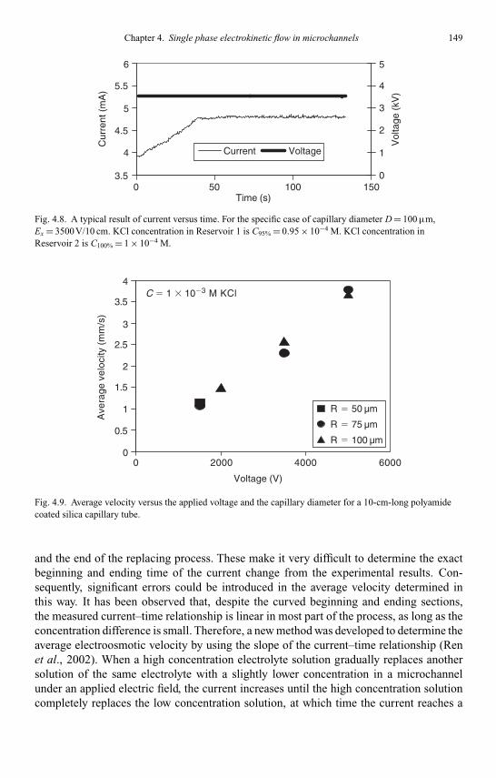
Kandlikar I044527-Ch04.tex 28/10/2005 16: 47 Page 149
Chapter 4. Single phase electrokinetic flow in microchannels 149
3.5
4
4.5
5
5.5
6
0 50 100 150Time (s)
Cur
rent
(m
A)
0
1
2
3
4
5
Vol
tage
(kV
)
Current Voltage
Fig. 4.8. A typical result of current versus time. For the specific case of capillary diameter D = 100 µm,Ex = 3500V/10 cm. KCl concentration in Reservoir 1 is C95% = 0.95 × 10⁻⁴ M. KCl concentration inReservoir 2 is C100% = 1 × 10⁻⁴ M.
Voltage (V)
Ave
rage
vel
ocity
(m
m/s
)
0
0.5
1
1.5
2
2.5
3
3.5
0 2000 4000 6000
4C � 1 10�3 M KCl
R � 50 µm
R � 75 µm
R � 100 µm
Fig. 4.9. Average velocity versus the applied voltage and the capillary diameter for a 10-cm-long polyamidecoated silica capillary tube.
and the end of the replacing process. These make it very difficult to determine the exactbeginning and ending time of the current change from the experimental results. Con-sequently, significant errors could be introduced in the average velocity determined inthis way. It has been observed that, despite the curved beginning and ending sections,the measured current–time relationship is linear in most part of the process, as long as theconcentration difference is small. Therefore, a new method was developed to determine theaverage electroosmotic velocity by using the slope of the current–time relationship (Renet al., 2002). When a high concentration electrolyte solution gradually replaces anothersolution of the same electrolyte with a slightly lower concentration in a microchannelunder an applied electric field, the current increases until the high concentration solutioncompletely replaces the low concentration solution, at which time the current reaches a
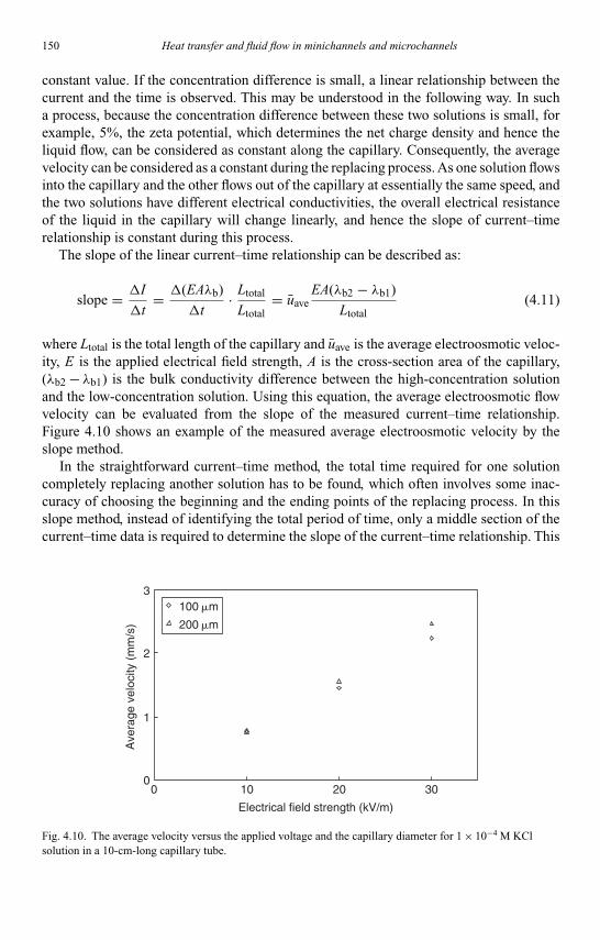
Kandlikar I044527-Ch04.tex 28/10/2005 16: 47 Page 150
150 Heat transfer and fluid flow in minichannels and microchannels
constant value. If the concentration difference is small, a linear relationship between thecurrent and the time is observed. This may be understood in the following way. In sucha process, because the concentration difference between these two solutions is small, forexample, 5%, the zeta potential, which determines the net charge density and hence theliquid flow, can be considered as constant along the capillary. Consequently, the averagevelocity can be considered as a constant during the replacing process. As one solution flowsinto the capillary and the other flows out of the capillary at essentially the same speed, andthe two solutions have different electrical conductivities, the overall electrical resistanceof the liquid in the capillary will change linearly, and hence the slope of current–timerelationship is constant during this process.
The slope of the linear current–time relationship can be described as:
slope = I
t= (EAλb)
t· Ltotal
Ltotal= uave
EA(λb2 − λb1)
Ltotal(4.11)
where Ltotal is the total length of the capillary and uave is the average electroosmotic veloc-ity, E is the applied electrical field strength, A is the cross-section area of the capillary,(λb2 − λb1) is the bulk conductivity difference between the high-concentration solutionand the low-concentration solution. Using this equation, the average electroosmotic flowvelocity can be evaluated from the slope of the measured current–time relationship.Figure 4.10 shows an example of the measured average electroosmotic velocity by theslope method.
In the straightforward current–time method, the total time required for one solutioncompletely replacing another solution has to be found, which often involves some inac-curacy of choosing the beginning and the ending points of the replacing process. In thisslope method, instead of identifying the total period of time, only a middle section of thecurrent–time data is required to determine the slope of the current–time relationship. This
0
1
2
3
0 10 20 30
Electrical field strength (kV/m)
Ave
rage
vel
ocity
(m
m/s
)
100 �m
200 �m
Fig. 4.10. The average velocity versus the applied voltage and the capillary diameter for 1 × 10⁻⁴ M KClsolution in a 10-cm-long capillary tube.
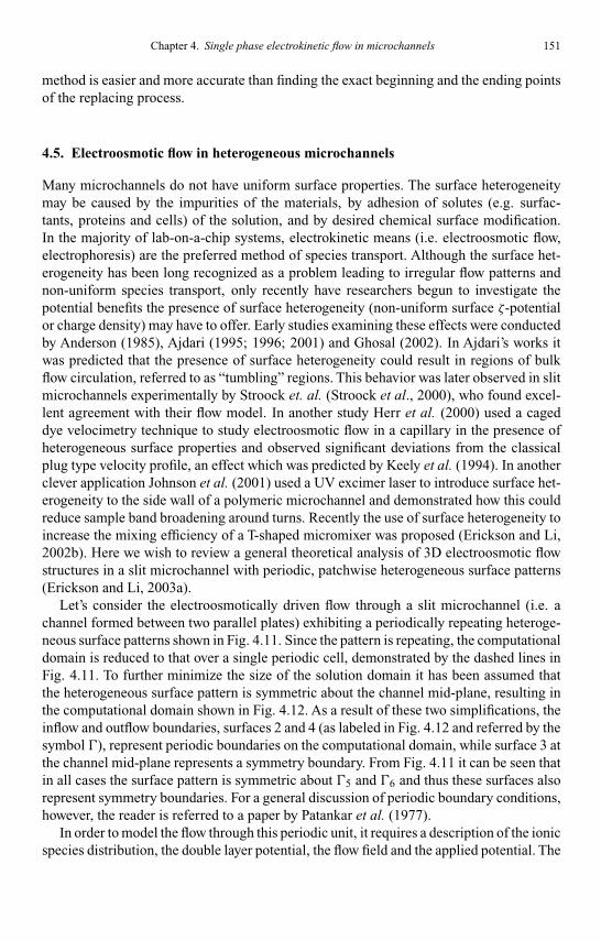
Kandlikar I044527-Ch04.tex 28/10/2005 16: 47 Page 151
Chapter 4. Single phase electrokinetic flow in microchannels 151
method is easier and more accurate than finding the exact beginning and the ending pointsof the replacing process.
4.5. Electroosmotic flow in heterogeneous microchannels
Many microchannels do not have uniform surface properties. The surface heterogeneitymay be caused by the impurities of the materials, by adhesion of solutes (e.g. surfac-tants, proteins and cells) of the solution, and by desired chemical surface modification.In the majority of lab-on-a-chip systems, electrokinetic means (i.e. electroosmotic flow,electrophoresis) are the preferred method of species transport. Although the surface het-erogeneity has been long recognized as a problem leading to irregular flow patterns andnon-uniform species transport, only recently have researchers begun to investigate thepotential benefits the presence of surface heterogeneity (non-uniform surface ζ-potentialor charge density) may have to offer. Early studies examining these effects were conductedby Anderson (1985), Ajdari (1995; 1996; 2001) and Ghosal (2002). In Ajdari’s works itwas predicted that the presence of surface heterogeneity could result in regions of bulkflow circulation, referred to as “tumbling” regions. This behavior was later observed in slitmicrochannels experimentally by Stroock et. al. (Stroock et al., 2000), who found excel-lent agreement with their flow model. In another study Herr et al. (2000) used a cageddye velocimetry technique to study electroosmotic flow in a capillary in the presence ofheterogeneous surface properties and observed significant deviations from the classicalplug type velocity profile, an effect which was predicted by Keely et al. (1994). In anotherclever application Johnson et al. (2001) used a UV excimer laser to introduce surface het-erogeneity to the side wall of a polymeric microchannel and demonstrated how this couldreduce sample band broadening around turns. Recently the use of surface heterogeneity toincrease the mixing efficiency of a T-shaped micromixer was proposed (Erickson and Li,2002b). Here we wish to review a general theoretical analysis of 3D electroosmotic flowstructures in a slit microchannel with periodic, patchwise heterogeneous surface patterns(Erickson and Li, 2003a).
Let’s consider the electroosmotically driven flow through a slit microchannel (i.e. achannel formed between two parallel plates) exhibiting a periodically repeating heteroge-neous surface patterns shown in Fig. 4.11. Since the pattern is repeating, the computationaldomain is reduced to that over a single periodic cell, demonstrated by the dashed lines inFig. 4.11. To further minimize the size of the solution domain it has been assumed thatthe heterogeneous surface pattern is symmetric about the channel mid-plane, resulting inthe computational domain shown in Fig. 4.12. As a result of these two simplifications, theinflow and outflow boundaries, surfaces 2 and 4 (as labeled in Fig. 4.12 and referred by thesymbol �), represent periodic boundaries on the computational domain, while surface 3 atthe channel mid-plane represents a symmetry boundary. From Fig. 4.11 it can be seen thatin all cases the surface pattern is symmetric about �5 and �6 and thus these surfaces alsorepresent symmetry boundaries. For a general discussion of periodic boundary conditions,however, the reader is referred to a paper by Patankar et al. (1977).
In order to model the flow through this periodic unit, it requires a description of the ionicspecies distribution, the double layer potential, the flow field and the applied potential. The
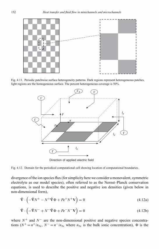
Kandlikar I044527-Ch04.tex 28/10/2005 16: 47 Page 152
152 Heat transfer and fluid flow in minichannels and microchannels
Fig. 4.11. Periodic patchwise surface heterogeneity patterns. Dark regions represent heterogeneous patches,light regions are the homogeneous surface. The percent heterogeneous coverage is 50%.
Direction of applied electric field
Iz
Iy
Ix
�
�
�
�
��3
y
x
z
Fig. 4.12. Domain for the periodical computational cell showing location of computational boundaries.
divergence of the ion species flux (for simplicity here we consider a monovalent, symmetricelectrolyte as our model species), often referred to as the Nernst–Planck conservationequations, is used to describe the positive and negative ion densities (given below innon-dimensional form),
∇ ·(−∇N+ − N+∇�+ Pe+N+V
)= 0 (4.12a)
∇ ·(−∇N− + N−∇�+ Pe−N−V
)= 0 (4.12b)
where N+ and N− are the non-dimensional positive and negative species concentra-tions (N+ = n+/n∞, N− = n−/n∞ where n∞ is the bulk ionic concentration), � is the

Kandlikar I044527-Ch04.tex 28/10/2005 16: 47 Page 153
Chapter 4. Single phase electrokinetic flow in microchannels 153
non-dimensional electric field strength (�= eφ/kbT where e is the elemental charge, kbis the Boltzmann constant and T is the temperature in Kelvin), V is the non-dimensionalvelocity (V = v/vo where vo is a reference velocity) and the ∼ sign signifies that thegradient operator has been non-dimensionalised with respect to the channel half height(ly in Fig. 4.12). The Peclet number for the two species are given by Pe+ = voly/D+ andPe− = voly/D− where D+ and D− are the diffusion coefficients for the positively chargedand negatively charged species respectively.
Along the heterogeneous surface (�1 in Fig. 4.12) and symmetry boundaries of thecomputational domain (�3, �5 and �6), zero flux boundary conditions are applied to bothEqs. (4.12a) and (b) (see reference (Erickson and Li, 2002a, b) for explicit equations). Asmentioned earlier, along faces �2 and �4, periodic conditions are applied which take theform shown below:
N+2 = N+
4 , on �2,�4, N−2 = N−
4 , on �2,�4
The velocity field is described by the Navier–Stokes equations for momentum, modifiedto account for the electrokinetic body force, and the continuity equation as shown below:
Re(V · ∇V) = −∇P + ∇2V − F(N+ − N−)∇� (4.13a)
∇ · V = 0 (4.13b)
where F is a non-dimensional constant (F = n∞lykbT /µvo) which accounts for the elec-trokinetic body force, Re is the Reynolds Number (Re = ρvoly/µ, where ρ is the fluiddensity and µ is the viscosity) and P is the non-dimensional pressure. Along the het-erogeneous surface, �1, a no-slip boundary condition is applied. At the upper symmetrysurface, �3, we enforce a zero penetration condition for the y-component of velocity andzero gradient conditions for the x and z terms, respectively. Similarly a zero penetrationcondition for the z-component of velocity is applied along �5 and �6 while zero gradientconditions are enforced for the x and y components. As with the Nernst–Planck equations,periodic boundary conditions are applied along �2 and �4.
For the potential field, we choose to separate, without loss of generality, the totalnon-dimensional electric field strength, �, into two components
�(X , Y , Z) = �(X , Y , Z) + E(X ) (4.14)
where the first component, �(X , Y , Z), describes the EDL field and the second componentE(X ) represents the applied electric field. In this case the gradient of E(X ) is of similarorder of magnitude to the gradient of�(X , Y , Z) and thus cannot be decoupled to simplifythe solution to the Poisson equation. As a result for this case the Poisson equation has theform shown below:
∇2� + d2E/ d X 2 + K2(N+ − N−) = 0 (4.15a)
where K is the non-dimensional double layer thickness (K2 = κ2l2y /2 where κ=
(2n∞e2/εwkbT )1/2 is the Debye–Huckel parameter). Two boundary conditions commonly

Kandlikar I044527-Ch04.tex 28/10/2005 16: 47 Page 154
154 Heat transfer and fluid flow in minichannels and microchannels
applied along the solid surface for the above equation are either an enforced potential gra-dient proportional to the surface charge density, or a fixed potential condition equivalentto the surface ζ-potential. In this case we choose the former resulting in the followingboundary condition applied along the heterogeneous surface
∂�/∂Y = −�(X , Z) on �1 (4.15b)
where � is the non-dimensional surface charge density (�= σlye/εwkbT , where σ is thesurface charge density). Along the upper and side boundaries of the computational domain,�3, �5 and �6, symmetry conditions are applied while periodic conditions are again areapplied at the inlet and outlet, �2 and �4.
In order to determine the applied electric field, E(X ), we enforce a constant currentcondition at each cross-section along the x-axis as below:
Jconst =Zmax∫0
Ymax∫0
[J +(X , Y , Z) − J −(X , Y , Z)]nx dY dZ (4.16a)
where nx in the above is a normal vector in the x-direction and J + and J − are the non-dimensional positive and negative current densities. Assuming monovalent ions for bothpositive and negative species (as was discussed earlier) and using the ionic species fluxterms from Eqs. (4.12a) and (b), condition 4.16(a) reduces to the following:
Jconst =Zmax∫0
Ymax∫0
(−[∂N+
∂X− Pe+
Pe−∂N−
∂X
]−[
N+ + Pe+
Pe− N−]∂(� + E)
∂X
)dY dZ
+Zmax∫0
Ymax∫0
[Pe+(N+ − N−)Vx]dY dZ (4.16b)
which is a balance between the conduction (term 2) and convection (term 3) currentswith an additional term to account for any induced current due to concentration gradients.Solving Eq. (4.16b) for the applied potential gradient yields:
dE
dX=
Zmax∫0
Ymax∫0
(−[∂N+∂X − Pe+
Pe−∂N−∂X
]−[N+ + Pe+
Pe− N−]∂�∂X
)dY dZ
Zmax∫0
Ymax∫0
(N+ + Pe+
Pe− N−)
dY dZ
+
Zmax∫0
Ymax∫0
[Pe+ (N+ − N−)Vx
]dY dZ − Jconst
Zmax∫0
Ymax∫0
(N+ + Pe+
Pe− N−)
dY dZ
(4.16c)

Kandlikar I044527-Ch04.tex 28/10/2005 16: 47 Page 155
Chapter 4. Single phase electrokinetic flow in microchannels 155
As an example, let us consider a lx = 50 µm, ly = lz = 25 µm computational domain,as shown in Fig. 4.12, containing a 10−5 M KCl solution and with an applied drivingvoltage of 500V/cm and a σhomo = −4 × 10⁻⁴ C/m2. The numerical simulations of theabove described model revealed three distinct flow patterns, depending on the degree ofsurface heterogeneity, as shown in Fig. 4.13. The grey scales in these figures representthe magnitude of the velocity perpendicular to the direction of the applied electric field(v2 = v2
y + v2z ) scaled by the maximum velocity in a homogeneous channel, which in this
example is 1.7 mm/s.At low degrees of surface heterogeneity (σhetero = −2 × 10⁻⁴ C/m2) the streamline pat-
tern shown in Fig. 4.13(a) was obtained. As can be seen a net counter-clockwise flowperpendicular to the applied electric field is present at the first transition plane (i.e. atthe initial discontinuity in the heterogeneous surface pattern) and a clockwise flow at thesecond transition plane. This flow circulation is a pressure-induced effect. It results fromthe transition from the higher local fluid velocity (particularly in the double layer) regionover the homogeneous surface on the right-hand side at the entrance to the left-hand sideafter the first transition plane (and vice versa at the second transition plane). To satisfycontinuity then there must be a net flow from right to left at this point, which in this casetakes the form of the circulation discussed above. The relatively straight streamlines par-allel with the applied electric field indicate that at this level the heterogeneity is too weakto significantly disrupt the main flow.
While a similar circulation pattern at the transition planes was observed as the degreeof surface heterogeneity was increased into the intermediate range (−2 × 10⁻⁴ C/m2 =σhetero = +2 × 10⁻⁴ C/m2), it is apparent from the darker contours shown in Fig. 4.13(b)that the strength of the flow perpendicular to the applied electric field is significantlystronger reaching nearly 50% of the velocity in the homogeneous channel. Unlike in theprevious case it is now apparent that the streamlines parallel with the applied electric fieldare significantly distorted due to the much slower or even oppositely directed velocity overthe heterogeneous patch.
At even higher degrees of heterogeneity (+2 × 10⁻⁴ C/m2 = σhetero = +4 × 10⁻⁴ C/m2)a third flow structure is observed in which a dominant circulatory flow pattern exists alongall three coordinate axes, as shown in Fig. 4.13(c). This results in a negligible, or even non-existent, bulk flow in the direction of the applied electric field (which is to be expected sincethe average surface charge density for these cases is very near zero). As indicated by thegrey scales, the velocity perpendicular to the flow axis has again increased in magnitude,reaching a maximum at the edge of the double layer near the symmetry planes at thelocation where a step change in the surface charge density has been imposed.
It is also shown (Erickson and Li, 2003a) that the induced 3D flow patterns are limited toa layer near the surface with a thickness equivalent to the length scale of the heterogeneouspatch. Additionally, the effect becomes smaller in magnitude and more localized as theaverage size of the heterogeneous region decreases. Moreover, it was demonstrated thatwhile convective effects are small, the electrophoretic influence of the applied electric fieldcould distort the net charge density field near the surface, resulting in a significant deviationfrom the traditional Poisson–Boltzmann double layer distribution. That is the reason whythe Nernst–Planck conservation equations, instead of the Boltzmann distribution equation,were used in this study.
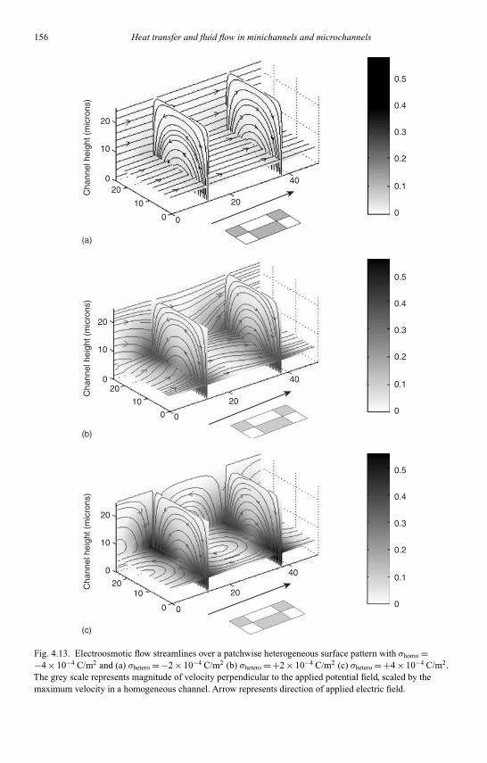
Kandlikar I044527-Ch04.tex 28/10/2005 16: 47 Page 156
156 Heat transfer and fluid flow in minichannels and microchannels
(a)
(b)
(c)
20
Cha
nnel
hei
ght (
mic
rons
)
2020
40
10
10
0
0 0
20
Cha
nnel
hei
ght (
mic
rons
)
20
20
10
10
0
0 0
20
0
0.1
0.2
0.3
0.4
0.5
0
0.1
0.2
0.3
0.4
0.5
0
0.1
0.2
0.3
0.4
0.5
Cha
nnel
hei
ght (
mic
rons
)
2020
40
40
10
10
0
0 0
Fig. 4.13. Electroosmotic flow streamlines over a patchwise heterogeneous surface pattern with σhomo =−4 × 10⁻⁴ C/m2 and (a) σhetero = −2 × 10⁻⁴ C/m2 (b) σhetero = +2 × 10⁻⁴ C/m2 (c) σhetero = +4 × 10⁻⁴ C/m2.The grey scale represents magnitude of velocity perpendicular to the applied potential field, scaled by themaximum velocity in a homogeneous channel. Arrow represents direction of applied electric field.

Kandlikar I044527-Ch04.tex 28/10/2005 16: 47 Page 157
Chapter 4. Single phase electrokinetic flow in microchannels 157
4.6. AC electroosmotic flow
Electroosmotic flow induced by unsteady applied electric fields or electroosmotic flowunder an alternating electrical (AC) field has its unique features and applications. Oddyet al. (2001) proposed and experimentally demonstrated a series of schemes for enhancedspecies mixing in microfluidic devices using AC electric fields. In addition Oddy et al.(2001) also presented an analytical flow field model, based on a surface slip conditionapproach, for an axially applied (i.e. along the flow axis) AC electric field in an infinitelywide microchannel. Comprehensive models for such a slit channel have also been pre-sented by Dutta and Beskok (2001), who developed an analytical model for an appliedsinusoidal electric field, and Söderman and Jönsson (1996), who examined the transientflow field caused by a series of different pulse designs. As an alternative to traditional DCelectroosmosis, a series of novel techniques have been developed to generate bulk flowusing AC fields. For example Green et al. (2000) experimentally observed peak flow veloc-ities on the order of hundreds of micrometers per second near a set of parallel electrodessubject to two AC fields, 180◦ out-of-phase with each other. The effect was subsequentlymodeled using a linear double layer analysis by Gonzàlez et al. (2000). Using a similarprincipal, both Brown et al. (2002) and Studer et al. (2002) presented microfluidic devicesthat incorporated arrays of non-uniformly sized embedded electrodes which, when subjectto an AC field, were able to generate a bulk fluid motion. Also using embedded electrodes,Selvaganapathy et al. (2002) demonstrated what they termed fr-EOF or bubble-free elec-troosmotic flow in which a creative periodic waveform was used to yield a net bulk flowwhile electrolytic bubble formation was theoretically eliminated.
Recently, Erickson and Li presented a combined theoretical and numerical approach toinvestigate the time periodic electroosmotic flow in a rectangular microchannel (Ericksonand Li, 2003b). This work considers the time-periodic electroosmotic flow in a straight,rectangular microchannel. Assuming a fully developed flow field and considering thegeometric symmetry, the analytical domain can be reduced to the upper left-hand quadrantof the channel cross-section as shown in Fig. 4.14. For pure electroosmotic flows (i.e. absent
ly
lx
X
Y
Analyticaldomain
O
z1
z2
Fig. 4.14. Illustration of the analytical domain in AC electroosmotic flow in a rectangular microchannel.

Kandlikar I044527-Ch04.tex 28/10/2005 16: 47 Page 158
158 Heat transfer and fluid flow in minichannels and microchannels
of any pressure gradients) of incompressible liquids, the Navier–Stokes equations may takethe following form:
ρf∂v
∂t= µ∇2v + ρeE(ωt) (4.17)
where v is the flow velocity, t is time, ρf is the fluid density, ρe is the net charge density,µ is the fluid viscosity and E(ωt) is a general time-periodic function with a frequencyω= 2πf and describes the applied electric field strength. To solve this flow equation, wemust know the local net charge density ρe. This requires solving the EDL field. Intro-ducing the non-dimensional double layer potential, �= zeψ/kbT , and non-dimensionaldouble layer thickness K = Dhκ (where Dh is the hydraulic diameter of the channel,Dh = 4lxly/2(lx + ly), and κ is the Deybe–Hückel parameter). We obtain the non-linearPoisson–Boltzmann distribution equation:
∇2� − K2 sinh� = 0 (4.18)
where the ∼ signifies that the spatial variables in the gradient operator have been non-dimensionalized with respect to Dh (i.e. X = x/Dh, Y = y/Dh). Eq. (4.18) is subject to thesymmetry conditions along the channel center axes, that is,
∂�/∂X = 0 at X = 0 ∂�/∂Y = 0 at Y = 0,
and the appropriate conditions at the channel walls,
� = Z1 at X = Lx/2 � = Z2 at Y = Ly/2
where Z1,2 = zeζ1,2/kbT , Lx = lx/Dh and Ly = ly/Dh.Generally, for multi-dimensional space and complex geometry Eq. (4.18) must be solved
numerically. However, under the condition that the double layer potential, �= zeψ/kbT ,is small, Eq. (4.18) can be linearized (the so-called the Deybe–Hückel approximation),yielding,
∇2� − K2� = 0 (4.19)
The Deybe–Hückel approximation is considered valid only when |zeζ|< kbT , which inprincipal is limited to cases where |ζ| ≤ 25 mV at room temperature. For the rectan-gular geometry shown in Fig. 4.14 an analytical solution to Eq. (4.19), subject to theaforementioned boundary conditions, can be obtained using a separation of variablestechnique:
�(X , Y ) =∞∑
n=1
4(−1)n+1
π(2n − 1)
[Z1 cos(λnX )
cosh([λ2n + K2]1/2Y )
cosh([λ2n + K2]1/2LY )
]
+∞∑
n=1
4(−1)n+1
π(2n − 1)
[Z2 cos(µnY )
cosh([µ2n + K2]1/2X )
cosh([µ2n + K2]1/2LX )
](4.20)
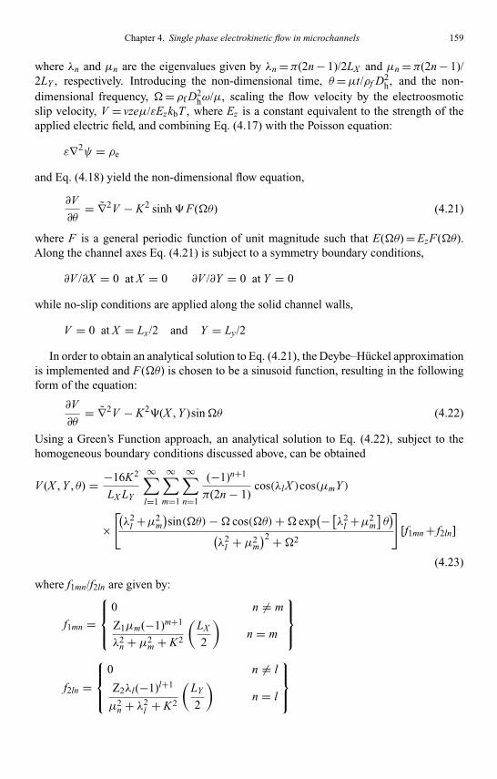
Kandlikar I044527-Ch04.tex 28/10/2005 16: 47 Page 159
Chapter 4. Single phase electrokinetic flow in microchannels 159
where λn and µn are the eigenvalues given by λn =π(2n − 1)/2LX and µn =π(2n − 1)/2LY , respectively. Introducing the non-dimensional time, θ=µt/ρf D2
h, and the non-dimensional frequency, �= ρf D2
hω/µ, scaling the flow velocity by the electroosmoticslip velocity, V = vzeµ/εEzkbT , where Ez is a constant equivalent to the strength of theapplied electric field, and combining Eq. (4.17) with the Poisson equation:
ε∇2ψ = ρe
and Eq. (4.18) yield the non-dimensional flow equation,
∂V
∂θ= ∇2V − K2 sinh�F(�θ) (4.21)
where F is a general periodic function of unit magnitude such that E(�θ) = EzF(�θ).Along the channel axes Eq. (4.21) is subject to a symmetry boundary conditions,
∂V /∂X = 0 at X = 0 ∂V /∂Y = 0 at Y = 0
while no-slip conditions are applied along the solid channel walls,
V = 0 at X = Lx/2 and Y = Ly/2
In order to obtain an analytical solution to Eq. (4.21), the Deybe–Hückel approximationis implemented and F(�θ) is chosen to be a sinusoid function, resulting in the followingform of the equation:
∂V
∂θ= ∇2V − K2�(X , Y )sin�θ (4.22)
Using a Green’s Function approach, an analytical solution to Eq. (4.22), subject to thehomogeneous boundary conditions discussed above, can be obtained
V (X , Y , θ) = −16K2
LX LY
∞∑l=1
∞∑m=1
∞∑n=1
(−1)n+1
π(2n − 1)cos(λlX )cos(µmY )
×[(λ2
l +µ2m
)sin(�θ)−� cos(�θ)+� exp
(− [λ2l +µ2
m
]θ)
(λ2
l + µ2m
)2 +�2
][f1mn + f2ln]
(4.23)
where f1mn/f2ln are given by:
f1mn =
0 n �= m
Z1µm(−1)m+1
λ2n + µ2
m + K2
(LX
2
)n = m
f2ln =
0 n �= l
Z2λl(−1)l+1
µ2n + λ2
l + K2
(LY
2
)n = l

Kandlikar I044527-Ch04.tex 28/10/2005 16: 47 Page 160
160 Heat transfer and fluid flow in minichannels and microchannels
Equation (4.23) represents the full solution to the transient flow problem. The equationcan be somewhat simplified in cases where the quasi-steady state time periodic solution(i.e. after the influence of the initial conditions has dissipated) is of interest. As these initialeffects are represented by the exponential term in Eq. (4.23), the quasi-steady state timeperiodic solution has the form shown below:
V (X , Y , θ) = −16K2
LX LY
∞∑l=1
∞∑m=1
∞∑n=1
(−1)n+1
π(2n − 1)cos(λlX )cos(µmY )
×[(λ2
l + µ2m
)sin(�θ)−� cos(�θ)(
λ2l + µ2
m
)2 +�2
][ f1mn + f2ln] (4.24)
In the above analytical description of the uniaxial electroosmotic flow in a rectangu-lar microchannel, the governing parameter is � which represents the ratio of the diffusiontime scale (tdiff = ρf D2
h/µ) to the period of the applied electric field (tE = 1/ω). Figure 4.15compares the time-periodic velocity profiles (as computed from Eq. (4.24)) in the upperleft-hand quadrant of a square channel for two cases: (a) �= 31 and (b) �= 625. Thesetwo � values correspond to frequencies of 500 Hz and 10 kHz in a 100 µm square chan-nel or equivalently a 100 µm and a 450 µm square channel at 500 Hz. To illustrate theessential features of the velocity profile a relatively large double layer thickness has beenused, κ= 3 × 10⁶ m−1 (corresponding to a bulk ionic concentration n∞ = 10−6 M), and auniform surface potential of ζ= −25 mV was selected (within the bounds imposed by theDeybe–Hückel linearization).
From Fig. 4.15, it is apparent that the application of the electrical body force results in arapid acceleration of the fluid within the double layer. In the case where the diffusion timescale is much greater than the oscillation period (high �, Fig. 4.15(b)) there is insufficienttime for fluid momentum to diffuse far into the bulk flow and thus while the fluid within thedouble layer oscillates rapidly the bulk fluid remains almost stationary. At �= 31 there ismore time for momentum diffusion from the double layer, however the bulk fluid still lagsbehind the flow in the double layer (this out-of-phase behavior will be discussed shortly).Extrapolating from these results, when �< 1, such that momentum diffusion is fasterthan the period of oscillation, the plug type velocity profile characteristic of steady stateelectroosmotic flow would be expected at all times.
Another interesting feature of the velocity profiles shown in Fig. 4.15 is the local velocitymaximum observed near the corner (most clearly visible in the �= 625 case at t =π/2ωand t =π/ω). The intersection of the two walls results in a region of double layer overlapand thus an increased net charge density over that region in the double layer. This peak in thenet charge density corresponds to a larger electrical body force and hence a local maximumelectroosmotic flow velocity, it also increases the ratio of the electrical body force to the vis-cous retardation allowing it to respond more rapidly to changes in the applied electric field.
The finite time required for momentum diffusion will inevitably result in some degreeof phase shift between the applied electric field and the flow response in the channel.From Fig. 4.15, however, it is apparent that within the limit of �> 1, this phase shift issignificantly different in the double layer region than in the bulk flow. It is apparent thatthe response of the fluid within the double layer to the AC field is essentially immediate,

Kandlikar I044527-Ch04.tex 28/10/2005 16: 47 Page 161
Chapter 4. Single phase electrokinetic flow in microchannels 161
(a) (b)
1
0.5
Non
-dim
ensi
onal
vel
ocity
0.4
0.2
Y X
Y X Y X
Y X Y X
Y X Y X
Y X
0.2
0.4
0 0
0
�0.5
�1
1
0.5
Non
-dim
ensi
onal
vel
ocity
0.4
0.20.2
0.4
0 0
0
�0.5
�1
1
0.5
Non
-dim
ensi
onal
vel
ocity
0.4
0.20.2
0.4
0 0
0
�0.5
�1
1
0.5
Non
-dim
ensi
onal
vel
ocity
0.4
0.20.2
0.4
0 0
0
�0.5
�1
1
0.5
Non
-dim
ensi
onal
vel
ocity
0.4
0.20.2
0.4
0 0
0
�0.5
�1
1
0.5
Non
-dim
ensi
onal
vel
ocity
0.4
0.20.2
0.4
0 0
0
�0.5
�1
1
0.5
Non
-dim
ensi
onal
vel
ocity
0.4
0.20.2
0.4
0 0
0
�0.5
�1
1
0.5
Non
-dim
ensi
onal
vel
ocity
0.4
0.20.2
0.4
0 0
0
�0.5
�1
t � p/2v
t � pv
t � 2pv
t � 3p/2v
Fig. 4.15. Steady-state time periodic electroosmotic velocity profiles in a square microchannel at (a) �= 30and (b) �= 625 (equivalent to an applied electric field frequency of (a) 500 Hz and (b) 10 kHz in a 100 µmsquare channel).
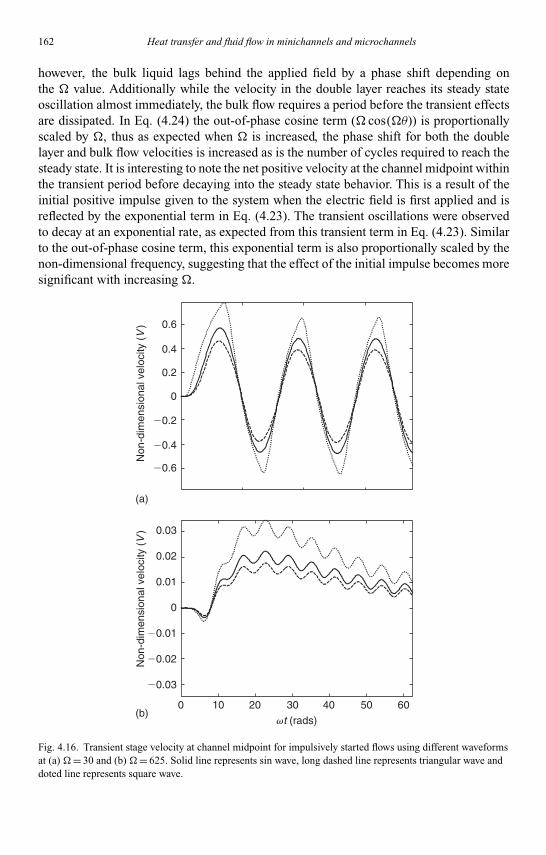
Kandlikar I044527-Ch04.tex 28/10/2005 16: 47 Page 162
162 Heat transfer and fluid flow in minichannels and microchannels
however, the bulk liquid lags behind the applied field by a phase shift depending onthe � value. Additionally while the velocity in the double layer reaches its steady stateoscillation almost immediately, the bulk flow requires a period before the transient effectsare dissipated. In Eq. (4.24) the out-of-phase cosine term (� cos(�θ)) is proportionallyscaled by �, thus as expected when � is increased, the phase shift for both the doublelayer and bulk flow velocities is increased as is the number of cycles required to reach thesteady state. It is interesting to note the net positive velocity at the channel midpoint withinthe transient period before decaying into the steady state behavior. This is a result of theinitial positive impulse given to the system when the electric field is first applied and isreflected by the exponential term in Eq. (4.23). The transient oscillations were observedto decay at an exponential rate, as expected from this transient term in Eq. (4.23). Similarto the out-of-phase cosine term, this exponential term is also proportionally scaled by thenon-dimensional frequency, suggesting that the effect of the initial impulse becomes moresignificant with increasing �.
0.4
0.6
0.2
0
Non
-dim
ensi
onal
vel
ocity
(V
)N
on-d
imen
sion
al v
eloc
ity (
V)
�0.2
�0.4
�0.6
(a)
(b)
0.03
0.02
0.01
0
0 10 20 30 40 50 60
�0.01
�0.02
�0.03
vt (rads)
Fig. 4.16. Transient stage velocity at channel midpoint for impulsively started flows using different waveformsat (a) �= 30 and (b) �= 625. Solid line represents sin wave, long dashed line represents triangular wave anddoted line represents square wave.
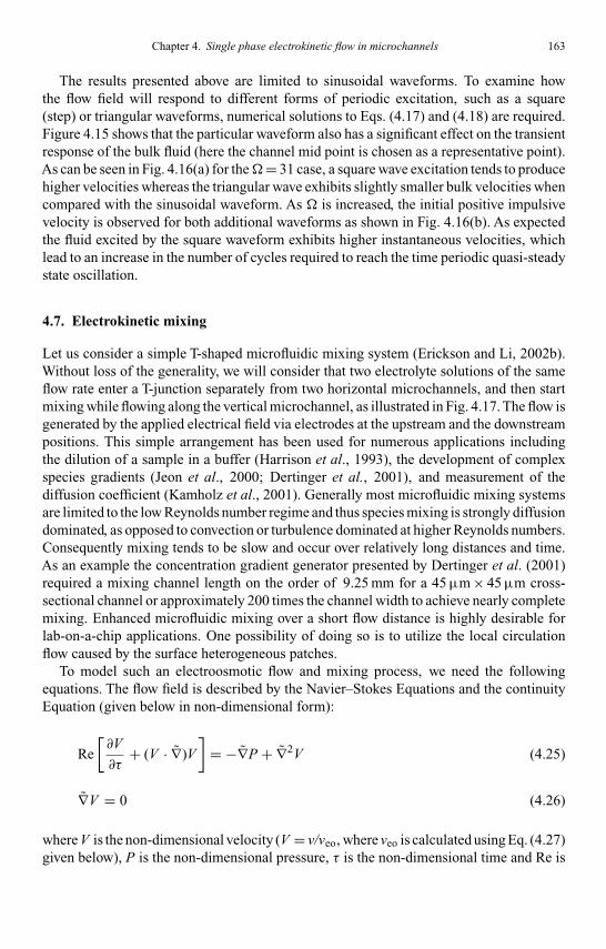
Kandlikar I044527-Ch04.tex 28/10/2005 16: 47 Page 163
Chapter 4. Single phase electrokinetic flow in microchannels 163
The results presented above are limited to sinusoidal waveforms. To examine howthe flow field will respond to different forms of periodic excitation, such as a square(step) or triangular waveforms, numerical solutions to Eqs. (4.17) and (4.18) are required.Figure 4.15 shows that the particular waveform also has a significant effect on the transientresponse of the bulk fluid (here the channel mid point is chosen as a representative point).As can be seen in Fig. 4.16(a) for the�= 31 case, a square wave excitation tends to producehigher velocities whereas the triangular wave exhibits slightly smaller bulk velocities whencompared with the sinusoidal waveform. As � is increased, the initial positive impulsivevelocity is observed for both additional waveforms as shown in Fig. 4.16(b). As expectedthe fluid excited by the square waveform exhibits higher instantaneous velocities, whichlead to an increase in the number of cycles required to reach the time periodic quasi-steadystate oscillation.
4.7. Electrokinetic mixing
Let us consider a simple T-shaped microfluidic mixing system (Erickson and Li, 2002b).Without loss of the generality, we will consider that two electrolyte solutions of the sameflow rate enter a T-junction separately from two horizontal microchannels, and then startmixing while flowing along the vertical microchannel, as illustrated in Fig. 4.17. The flow isgenerated by the applied electrical field via electrodes at the upstream and the downstreampositions. This simple arrangement has been used for numerous applications includingthe dilution of a sample in a buffer (Harrison et al., 1993), the development of complexspecies gradients (Jeon et al., 2000; Dertinger et al., 2001), and measurement of thediffusion coefficient (Kamholz et al., 2001). Generally most microfluidic mixing systemsare limited to the low Reynolds number regime and thus species mixing is strongly diffusiondominated, as opposed to convection or turbulence dominated at higher Reynolds numbers.Consequently mixing tends to be slow and occur over relatively long distances and time.As an example the concentration gradient generator presented by Dertinger et al. (2001)required a mixing channel length on the order of 9.25 mm for a 45 µm × 45 µm cross-sectional channel or approximately 200 times the channel width to achieve nearly completemixing. Enhanced microfluidic mixing over a short flow distance is highly desirable forlab-on-a-chip applications. One possibility of doing so is to utilize the local circulationflow caused by the surface heterogeneous patches.
To model such an electroosmotic flow and mixing process, we need the followingequations. The flow field is described by the Navier–Stokes Equations and the continuityEquation (given below in non-dimensional form):
Re[∂V
∂τ+ (V · ∇)V
]= −∇P + ∇2V (4.25)
∇V = 0 (4.26)
where V is the non-dimensional velocity (V = v/veo, where veo is calculated using Eq. (4.27)given below), P is the non-dimensional pressure, τ is the non-dimensional time and Re is

Kandlikar I044527-Ch04.tex 28/10/2005 16: 47 Page 164
164 Heat transfer and fluid flow in minichannels and microchannels
Inlet stream 2
Mixed stream
Inlet stream 1
Mixing channel
w
Larm
Lmix
w
X
Y
Fig. 4.17. T-Shaped micromixer formed by the intersection of two microchannels, showing a schematic of themixing or dilution process.
the Reynolds number given by Re = ρveoL/ηwhere L is a length scale taken as the channelwidth (w from Fig. 4.17) in this case. The ∼ symbol over the ∇ operator indicates thegradient with respect to the non-dimensional coordinates (X = x/w, Y = y/w and Z = z/w).
It should be noted that in order to simplify the numerical solution to the problem, wehave treated the electroosmotic flow in the thin EDL as a slip flow velocity boundarycondition, given by:
veo = µeo∇φ =(εwζ
µ
)∇φ (4.27)
where µeo = (εwζ/µ) is the electroosmotic mobility, εw is the electrical permittivity of thesolution, µ is the viscosity, ζ is the zeta potential of the channel wall, and φ is the appliedelectric field strength.
In general the high voltage requirements limit most practical electroosmotically drivenflows in microchannels to small Reynolds numbers, therefore to simplify Eq. (4.25) weignore transient and convective terms and limit ourselves to cases where Re< 0.1.
We consider the mixing of equal portions of two buffer solutions, one of which containsa species of interest at a concentration, co. Species transport by electrokinetic means isaccomplished by three mechanisms: convection, diffusion and electrophoresis, and can bedescribed by:
Pe[∂C
∂τ+ ∇ · (C(V + Vep))
]= ∇2C (4.28)

Kandlikar I044527-Ch04.tex 28/10/2005 16: 47 Page 165
Chapter 4. Single phase electrokinetic flow in microchannels 165
0
100
200
Dow
nstr
eam
dis
tanc
e (m
icro
ns)
(a) (b)
300
400
500
0
100
200
Dow
nstr
eam
dis
tanc
e (m
icro
ns)
300
400
500
Fig. 4.18. Electroosmotic streamlines at the mid-plane of a 50 µm T-shaped micromixer for the(a) homogeneous case with ζ= −42 mV, (b) heterogeneous case with six offset patches on the left-and right-channel walls. All heterogeneous patches are represented by the crosshatched regions andhave a ζ= + 42 mV. The applied voltage is φapp = 500V/cm.
where C is the non-dimensional species concentration (C = c/co, where co is originalconcentration of the interested species in the buffer solution.), Pe is the Péclet num-ber (Pe = veow/D, where D is the diffusion coefficient), and Vep is the non-dimensionalelectrophoretic velocity equal to vep/veo where vep is given by:
vep = µep∇φ (4.29)
and µep = (εwζp/η) is the electrophoretic mobility (εw is the electrical permittivity of thesolution, µ is the viscosity, ζp is the zeta potential of the to-be-mixed charged moleculesor particles) (Hunter, 1981). As we are interested in the steady state solution, the transientterm in Eq. (4.28) can be ignored.
The above described model was solved numerically to investigate the formation of elec-troosmotically induced flow circulation regions near surface heterogeneities in a T-shapedmicromixer and to determine the influence of these regions on the mixing effectiveness.In Fig. 4.18 we compare the mid-plane flow field near the T-intersection of a homoge-neous mixing channel with that of a mixing channel having a series of 6 asymmetrically

Kandlikar I044527-Ch04.tex 28/10/2005 16: 47 Page 166
166 Heat transfer and fluid flow in minichannels and microchannels
(a) (b)
Fig. 4.19. 3D species concentration field for a 50 µm × 50 µm T-shaped micromixer resulting from the flowfields shown in Fig. 4.23. (a) homogeneous case and (b) heterogeneous case with offset patches. Speciesdiffusivity is 3 × 10⁻¹⁰ m2/s and zero electrophoretic mobility are assumed.
distributed heterogeneous patches on the left- and right-channel walls. For clarity the het-erogeneous regions are marked as the crosshatched regions in this figure. The homogeneouschannel surface has a ζ potential of −42 mV. A ζ-potential of ζ= +42 mV was assumedfor the heterogeneous patches. Apparently, the channel with heterogeneous patches gener-ates local flow circulations near the patches. These flow circulation zones are expected toenhance the mixing of the two streams.
Figure 4.19 compares the 3D concentration fields of the homogeneous and hetero-geneous mixing channel shown in Fig. 4.18. In these figures a neutral mixing species(i.e. µep = 0, thereby ignoring any electrophoretic transport) with a diffusion coefficientD = 3 × 10⁻¹⁰ m2/s is considered. While mixing in the homogeneous case is purely dif-fusive in nature, the presence of the asymmetric circulation regions, Fig. 4.19(b), enablesenhanced mixing by convection.
Recently a passive electrokinetic micromixer based on the use of surface charge hetero-geneity was developed (Biddiss et al., 2004). The micromixer is a T-shaped microchannelstructure (200 µm in width and approximately 8 µm in depth) made from Polydimethyl-siloxane (PDMS) and is sealed with a glass slide. Microchannels were fabricated using arapid prototyping/soft-lithography technique. The glass surface was covered by a PDMSmask with the desired heterogeneous pattern, then treated with a Polybrene solution. Afterremoving the mask, the glass surface will have selective regions of positive surface chargewhile leaving the majority of the glass slide with its native negative charge (Biddiss et al.,2004). Finally the PDMS plate (with the microchannel structure) will be bonded to theglass slide to form the sealed, T-shaped microchannel with heterogeneous patches on themixing channel surface.
A micromixer consisting of 6 offset staggered patches (in the mixing channel) spanning1.8 mm downstream and offset 10 µm from the channel centerline with a width of 90 µm

Kandlikar I044527-Ch04.tex 28/10/2005 16: 47 Page 167
Chapter 4. Single phase electrokinetic flow in microchannels 167
(a) (b)
Fig. 4.20. Images of steady-state species concentration fields under an applied potential of 280V/cm for(a) the homogeneous microchannel and (b) the heterogeneous microchannel with six offset staggered patches.
and a length of 300 µm, was analyzed experimentally. Mixing experiments were conductedat applied voltage potentials ranging between 70 and 555V/cm and the correspondingReynolds numbers range from 0.08 to 0.7 and Péclet numbers from 190 to 1500. The liquidis a 25 mM sodium carbonate/bicarbonate buffer. To visualize the mixing effects, 100 µMfluorescein was introduced through one inlet channel. As an example, Fig. 4.20 shows theexperimental images of the steady state flow for the homogenous and heterogeneous casesat 280V/cm. The enhanced mixing effect is obvious.
This experimental study shows that the passive electrokinetic micromixer with an opti-mized arrangement of surface charge heterogeneities can increase flow narrowing andcirculation, thereby increasing the diffusive flux and introducing an advective componentof mixing. Mixing efficiencies were improved by 22–68% for voltages ranging from 70to 555V/cm. For producing a 95% mixture, this technology can reduce the required mix-ing channel length of up to 88% for flows with Péclet numbers between 190 and 1500,and Reynolds numbers between 0.08 and 0.7. In terms of required channel lengths, at280V/cm, a homogeneous microchannel would require a channel mixing length of 22 mmfor reaching a 95% mixture. By implementing the developed micromixer, an 88% reduc-tion in required channel length to 2.6 mm was experimentally demonstrated. Practicalapplications of reductions in required channel lengths include improvements in portabilityand shorter retention times, both of which are valuable advancements applicable to manymicrofluidic devices.

Kandlikar I044527-Ch04.tex 28/10/2005 16: 47 Page 168
168 Heat transfer and fluid flow in minichannels and microchannels
4.8. Electrokinetic sample dispensing
An important component of many bio- or chemical lab-chips is the microfluidic dispenser,which employs electroosmotic flow to dispense minute quantities (e.g. 300 pico-liters) ofsamples for chemical and biomedical analysis. The precise control of the dispensed samplein microfluidic dispensers is key to the performance of these lab-on-a-chip devices.
Let us consider a microfluidic dispenser formed by two crossing microchannels asshown in Fig. 4.21 (Ren and Li, 2002). The depth and the width of all the channels arechosen to be 20 µm and 50 µm, respectively. There are four reservoirs connected to thefour ends of the microchannels. Electrodes are inserted into these reservoirs to set upthe electrical field across the channels. Initially, a sample solution (a buffer solution withsample species) is filled in Reservoir 1, the other reservoirs and the microchannels arefilled with the pure buffer solution. When the chosen electrical potentials are applied to thefour reservoirs, the sample solution in Reservoir 1 will be driven to flow toward Reservoir3 passing through the intersection of the cross channels. This is the so-called loadingprocess. After the loading process reaches a steady state, the sample solution loaded inthe intersection will be “cut” or dispensed into the dispensing channel by the dispensingsolution flowing from Reservoir 2 to 4. This can be realized by adjusting the electricalpotentials applied to these four reservoirs. This is the so called the dispensing process.The volume and the concentration of the dispensed sample are the key parameters of thisdispensing process, and they depend on the applied electrical field, the flow field and theconcentration field during the loading and the dispensing processes.
To model such a dispensing process, we must model the applied electrical field, the flowfield and the concentration field. To simplify the analysis, we consider this as a 2D problem,
x
y
z
Wy
Wx
Reservoir 1 Reservoir 3
Reservoir 2
Reservoir 4
Fig. 4.21. The schematic diagram of a crossing microchannel dispenser. Wx and Wy indicate the width of themicrochannels.

Kandlikar I044527-Ch04.tex 28/10/2005 16: 47 Page 169
Chapter 4. Single phase electrokinetic flow in microchannels 169
that is, ignoring the variation in the z-direction. The 2D applied electrical potential in theliquid can be described by:
∂2φ∗
∂x∗2 + ∂2φ∗
∂y∗2 = 0
Here the non-dimensional parameters are defined by:
φ∗ = φ
�, x∗ = x
h, y∗ = y
h
where � is a reference electrical potential and h is the channel width chosen as 50 µm.Boundary conditions are required to solve this equation. We impose the insulation conditionto all the walls of microchannels, and the specific non-dimensional potential values to allthe reservoirs. Once the electrical field in the dispenser is known, the local electric fieldstrength can be calculated by
�E = −�∇�The electroosmotic flow field reaches steady state in milli-seconds, much shorter thanthe characteristic time scales of the sample loading and sample dispensing. Therefore, theelectroosmotic flow here is approximated as steady state. Furthermore, we consider athin EDL, and use the slip flow boundary condition to represent the electroosmotic flow.The liquid flow field can thus be described by the following non-dimensional momentumequation and the continuity equation:
u∗eo∂u∗
eo
∂x∗ + v∗eo∂u∗
eo
∂y∗ = −∂P∗
∂x∗ + ∂2u∗eo
∂x∗2 + ∂2u∗eo
∂y∗2
u∗eo∂v∗
eo
∂x∗ + v∗eo∂v∗
eo
∂y∗ = −∂P∗
∂y∗ + ∂2v∗eo
∂x∗2 + ∂2v∗eo
∂y∗2
∂u∗eo
∂x∗ + ∂v∗eo
∂y∗ = 0
where ueo, veo are the electroosmotic velocity component in x- and y-direction, respectively,and non-dimensionalized as follows:
P∗ = P − Pa
ρ(v/h)2 , u∗eo = ueoh
v, v∗
eo = veoh
v
The slip velocity conditions are applied to the walls of the microchannels, the fully devel-oped velocity profile is applied to all the interfaces between the microchannels and thereservoirs, and the pressures in the four reservoirs are assumed to be the atmosphericpressure.
The distribution of the sample concentration can be described by the conservation lawof mass, taking the following form:
∂C∗i
∂τ+(
u∗eo + u∗
ep
) ∂C∗i
∂x∗ +(
v∗eo + v∗
ep
) ∂C∗i
∂y∗ = Di
v
(∂2C∗
i
∂x∗2 + ∂2C∗i
∂y∗2
)

Kandlikar I044527-Ch04.tex 28/10/2005 16: 47 Page 170
170 Heat transfer and fluid flow in minichannels and microchannels
0.28
25
0.281
0.282
0.283
0.284
0.285
0.287
0.2895
0.291
0.2825
X (mm)
Y (
mm
)
2.45 2.5 2.55 2.69.95
10
10.05
10.1
R1
R4
R3
R2
X (mm)
Y (
mm
)
2.45 2.5 2.55 2.69.95
10
10.05
10.1
R1
R4
R3
R2
X (mm)
Y (
mm
)
2.45 2.5 2.55 2.69.95
10
10.05
10.1
R1
R4
R3
R2
0.48
5
0.49
0.47
4
0.47
6
0.47
8
0.48
0.46
5
0.47
X (mm)
Y (
mm
)
2.45 2.5 2.55 2.6
10
10.05
10.1R4
R1 R3
R29.95
Fig. 4.22. Examples of the applied electrical field (left) and the flow field (right) at the intersection of themicrochannels in a loading process (top) and in a dispensing process (bottom).
where Ci is the concentration of the ith species, ueo and veo are the components of theelectroosmotic velocity of the ith species, Di is the diffusion coefficient of the ith species,and uepi and vepi are the components of the electrophoretic velocity of the ith speciesgiven by uepi = Eµepi, where µepi is the electrophoretic mobility. The non-dimensionalparameters in the above equation are defined by C∗ = C/�C, and τ= t/(h2/v), where �C is areference concentration.
Figure 4.22 shows the typical electrical field and flow field (computer simulated) for theloading and dispensing process, respectively. In this figure, the non-dimensional appliedelectrical potentials are: φ∗(1) = 1.0, φ∗(2) = 1.0,φ∗(3) = 0.0,φ∗(4) =1.0 for the loadingprocess, and φ∗(1) = 0.2,φ∗(2) = 2.0,φ∗(3) = 0.2,φ∗(4) = 0.0 for the dispensing process,where φ∗(i) represents the non-dimensional applied electrical potential to ith reservoir.For this specific case, the electrical field and the flow field for the loading process aresymmetric to the middle line of the horizontal channel, and the electrical field and the flowfield for the dispensing process are symmetric to the middle line of the vertical channel.

Kandlikar I044527-Ch04.tex 28/10/2005 16: 47 Page 171
Chapter 4. Single phase electrokinetic flow in microchannels 171
(b)
(c)
(a)
Loading(steady state)
1 4
3
dispensing
Fig. 4.23. The loading and dispensing of a focused fluorescein sample: (a) Processed images;(b) iso-concentration profiles at 0.1Co, 0.3Co, 0.5Co, 0.7Co, and 0.9Co, calculated from the images and(c) corresponding iso-concentration profiles calculated through numerical simulation.
The electrokinetic dispensing processes of fluorescent dye samples were investigatedexperimentally (Sinton et al., 2003b, c, d). The measurements were conducted by usinga fluorescent dye-based microfluidic visualization system. Fig. 4.23 shows a sample dis-pensing process and the comparison of the dispensed sample concentration profile withthe numerically simulated results. Both the theoretical studies and the experimental stud-ies have demonstrated that the loading and dispensing of sub-nanolitre samples using amicrofluidic crossing microchannel chip can be controlled electrokinetically. The abilityto inject and transport large axial extent, concentration-dense samples was demonstrated.Both experimental and numerical results indicate the shape, cross-stream uniformity, andaxial extent of the samples were very sensitive to changes in the electric fields applied inthe loading channel. In the dispensing process, larger samples were shown to disperse lessthan focused samples, maintaining more solution with the original sample concentration.
4.9. Practice problems
1. Model and simulate 1D steady state electroosmotic flow in a circular capillary under anapplied DC field. Plot and discuss the EDL field and flow field, effects of zeta potential,bulk ionic concentration, applied voltage and diameter.
2. Model and simulate a 1D steady state electroosmotic flow in a microchannel under anapplied DC field and a small externally applied pressure difference along the channel.Plot and discuss the flow field in terms of the value and the direction of the appliedpressure gradient, zeta potential and the applied electrical field.

Kandlikar I044527-Ch04.tex 28/10/2005 16: 47 Page 172
172 Heat transfer and fluid flow in minichannels and microchannels
3. Model and simulate 1D electroosmotic flow in a circular capillary under an appliedAC field. Plot and discuss the flow field, effects of the zeta potential, the bulk ionicconcentration, the AC voltage and frequency, and diameter of the capillary.
4. Model and simulate a steady state electroosmotic flow in a microchannel with a 90degree turn under an applied DC field. Plot and discuss the flow field in terms of thezeta potential, the channel size and the applied electrical field.
5. Model and simulate electroosmotic flow in a converging–diverging circular microcapil-lary with a constant zeta potential, Plot the flow field (streamlines and velocity) and theinduced pressure field, and discuss the effects of the applied field strength, dimensionsof the converging–diverging microchannel, and the zeta potentials.
6. Model and simulate electroosmotic mixing of two aqueous solutions in a homogeneousT-shaped microchannel. Plot the flow field (streamlines and velocity) and the concen-tration field in the mixing channel, and discuss the effects of the applied field strengthsat the two inlets, the zeta potential and dimensions of the microchannel on the mixinglength (i.e. the length required to have 99% of mixing).
References
Ajdari, A., Elctroosmosis on inhomogeneously charged surfaces, Phys. Rev. Lett., 75, 755–758,1995.
Ajdari, A., Generation of transverse fluid currents and forces by an electric field: electro-osmosis oncharge-modulated and undulated surfaces, Phys. Rev. E., 53, 4996–5005, 1996.
Ajdari, A., Transverse electrokinetic and microfluidic effects in micropatterned channels: lubricationanalysis for slab geometries, Phys. Rev. E., 65, 016301, 2001.
Anderson, J. L., Effect of nonuniform zeta potential on particle movement in electricfields, J. ColloidInterface Sci., 105, 45–54, 1985.
Arulanandam, S. and Li, D., Liquid transport in rectangular microchannels by electroosmoticpumping, Colloid Surface A, 161, 89–102, 2000a.
Arulanandam, S. and Li, D., Evaluation of zeta potential and surface conductance by measuringelectro-osmotic current, J. Colloid Interface Sci., 225, 421–428, 2000b.
Biddiss, E., Erickson, D., and Li, D., Heterogeneous surface charge enhanced micro-mixing forelectrokinetic flows, Anal. Chem., 76, 3208–3213, 2004.
Brown, A. B. D., Smith, C. G., and Rennie, A. R., Pumping of water with an AC electric field appliedto asymmetric pairs of microelectrodes, Phys. Rev. E., 63, 016305 1–8, 2002.
Dahm, W. J. A., Su, L. K., and Southerland, K. B., A scalar imaging velocimetry technique for fullyresolved four-dimensional vector velocity field measurement in turbulent flows, Phys. fluid A, 4,2191–2206, 1992.
Dertinger, S. K. W., Chiu, D. T., Jeon, N. L., and Whitesides, G. M., Generation of gradients havingcomplex shapes using microfluidic networks, Anal. Chem., 73, 1240–1246, 2001.
Dutta, P. and Beskok, A., Analytical solution of time periodic electroosmotic flows: analogies tostokes second problem, Anal. Chem., 73, 5097–5102, 2001.
Erickson, D. and Li, D., Influence of surface heterogeneity on electrokinetically driven microfluidicmixing, Langmuir, 18, 8949–8959, 2002a.
Erickson, D. and Li, D., Microchannel flow with patch-wise and periodic surface heterogeneity,Langmuir, 18, 1883–1892, 2002b.
Erickson, D. and Li, D., Three dimensional structure of electroosmotic flows over periodicallyheterogeneous surface patterns, J. Phys. Chem. B., 107, 12212–12220, 2003a.

Kandlikar I044527-Ch04.tex 28/10/2005 16: 47 Page 173
Chapter 4. Single phase electrokinetic flow in microchannels 173
Erickson, D. and Li, D., Analysis of AC electroosmotic flows in a rectangular microchannel,Langmuir, 19, 5421–5430, 2003b.
Ghosal, S., Lubrication theory for electro-osmotic flow in a micrflouidic channel of slowly varyingcross-section and wall charge, J. Fluid. Mech., 459, 103–128, 2002.
Gonzàlez, A., Ramos, A., Green, N. G., Castellanos, A., and Morgan, H., Fluid flow induced by non-uniform AC electric fields in electrolytes on microelectrodes II: A linear double layer analysis,Phys. Rev. E., 61, 4019–4028, 2000.
Green, N. G., Ramos, A., Gonzàlez, A., Morgan, H., and Castellanos, A., Fluid flow induced bynon-uniform AC electric fields in electrolytes on microelectrodes I: experimental measurements,Phys. Rev. E., 61, 4011–4018, 2000.
Harrison, J. D., Fluri, K., Seiler, K., Fan, Z., Effenhauser, C., and Manz, A., Micromachining aminiaturized capillary electrophoresis-based chemical analysis system on a chip, Science, 261,895–897, 1993.
Herr, A. E., Molho, J. I., Santiago, J. G., Mungal, M. G., Kenny, T. W., and Garguilo, M. G.,Electroosmotic capillary flow with nonuniform zeta potential, Anal. Chem., 72, 1053–1057,2000.
Hunter, R. J., Zeta potential in colloid science: principle and applications, Academic Press, London:1981.
Jeon, N. L., Dertinger, S. K. W., Chiu, D. T., Choi, I. S., Stroock, A. D., and Whitesides, G.M.,Generation of solution and surface gradients using microfluidic systems, Langmuir, 16, 8311–8316, 2000.
Johnson, T. J., Ross, D., Gaitan, M., and Locascio, L. E., Laser modification of preformed polymermicrochannels: application to reduce band broadening around turns subject to electrokinetic flow,Anal. Chem., 73, 3656–3661, 2001.
Kamholz, A. E., Schilling, E. A., and Yager, P., Optical measurement of transverse moleculardiffusion in a microchannel, Biophys. J., 80, 1967–1972, 2001.
Keely, C. A., van de Goor, T. A. A., and McManigill, D., Modeling flow profiles and disper-sion in capillary electrophoresis with nonuniform zeta potential, Anal. Chem., 66, 4236–4242,1994.
Lempert, W. R., Magee, K., Ronney, P., Gee, K. R., and Haugland, R. P., Low tagging velocime-try in incompressible flow using photo-activated nonintrusive tracking of molecular motion(PHANTOMM), Exp. Fluids, 18, 249–257, 1995.
Li, D., Electrokinetics in microfluidics, Academic Press, London: 2004.Lyklema, J., Fundamentals of interface and colloid science, Vol. II, Solid–Liquid Interfaces,
Academic Press, London: 1995.Mala, G. M., Li, D., Werner, C., Jacobasch, H. J., and Ning, Y. B., Flow characteristics of water
through a microchannel between two parallel plates with electrokinetic effects, Int. J. Heat FluidFlow, 18, 489–496, 1997.
Meinhart, C. D., Wereley, S. T., and Santiago, J. D., PIV measurements of a microchannel flow, Exp.Fluid., 27, 414–419, 1999.
Molho, J. L., Herr, A. E., Mosier, B. P., Santiago, J. G., Kenny, T. W., Breenen, R. A., Gordon, G. B.,and Mohammadi, B., Optimization of turn geometries for microchip electrophoresis, Anal. Chem.,73, 1350–1360, 2001.
Oddy, M. H., Santiago, J. G., and Mikkelsen, J. C., Electrokinetic instability micromixing, Anal.Chem., 73, 5822–5832, 2001.
Patankar, S., Liu, C., and Sparrow, E., Fully developed flow and heat transfer in ducts havingstreamwise-periodic variation of cross-sectional area, J. Heat Trans., 99, 180–186, 1977.
Paul, P. H., Garguilo, M. G., and Rakestraw, D. J., Imaging of pressure- and electrokinetically drivenflows through open capillaries, Anal. Chem., 70, 2459–2467, 1998.

Kandlikar I044527-Ch04.tex 28/10/2005 16: 47 Page 174
174 Heat transfer and fluid flow in minichannels and microchannels
Ren, L. and Li, D., Theoretical studies of microfluidic dispensing processes, J. Colloid InterfaceSci., 254, 384–395, 2002.
Ren, L., Escobedo, C., and Li, D., Electro-osmotic flow in micro-capillary with one solutiondisplacing another solution, J. Colloid Interface Sci., 250, 238–242, 2002.
Reuss, E. F., Memoires de la societe imperiale des naturalistes de moskou., 2, 327, 1809.Santiago, J. G., Wereley, S. T., Meinhart, C. D., Beebe, D. J., and Adrian, R. J., A particle image
velocimetry system for microfluidics, Exp. Fluid., 25, 316–319, 1998.Selvaganapathy, P., Ki, Y. -S. L., Renaud, P., and Mastrangelo, C. H., Bubble-free electrokinetic
pumping, J. Microelectromech. Sys., 11, 448–453, 2002.Singh, A. K., Cummings, E. B., and Throckmorton, D. J., Fluorescent liposome flow markers for
microscale particle-image velocimetry, Anal. Chem., 73, 1057–1061, 2001.Sinton, D., Escobedo, C., Ren, L., and Li, D., Direct and indirect electroosmotic flow velocity
measurements in microchannels, J. Colloid Interface Sci., 254, 184–189, 2002.Sinton, D., Erickson, D., and Li, D., Micro-bubble lensing induced photobleaching (µ-BLIP) with
application to microflow visualization, Exp. Fluid., 35, 178–187, 2003.Sinton, D. and Li, D., Caged-dye based microfluidic velocimetry with near-wall resolution, Int.
J. Therm. Sci., 42, 847–855, 2003a.Sinton, D. and Li, D., Electroosmotic velocity profiles in microchannels, Colloid. Surfaces A., 222,
273–283, 2003b.Sinton, D., Ren, L., and Li, D., Visualization and numerical simulation of microfluidic on-chip
injection, J. Colloid Interface Sci., 260, 431–439, 2003.Sinton, D., Ren, L., and Li, D., A dynamic loading method for controlling on-chip microfluidic chip
sample injection, J. Colloid Interface Sci., 266, 448–456, 2003c.Sinton, D., Ren, L., Xuan, X., and Li, D., Effects of liquid conductivity differences on multi-
component sample injection, pumping and stacking in microfluidic chips, Lab-on-a-Chip, 3,173–179, 2003d.
Söderman, O. and Jönsson, B., Electro-osmosis: velocity profiles in different geometries with bothtemporal and spatial resolution, J. Chem. Phys., 105, 10300–10311, 1996.
Stroock, A. D., Weck, M., Chiu, D. T., Huck, W. T. S., Kenis, P. J. A., Ismagilov, R. F., andWhitesides, G. M., Patterning electro-osmotic flow with patterned surface charge, Phys. Rev.Lett., 84, 3314–3317, 2000.
Studer, V., Pépin, A., Chen, Y., and Ajdari, A., Fabrication of microfluidic devices for ACelectrokinetic fluid pumping, Microelectronic Eng., 61–62, 915–920, 2002.
Taylor, J. A. and Yeung, E. S., Imaging of hydrodynamic and electrokinetic flow profiles incapillaries, Anal. Chem., 65, 2928–2932, 1993.
Wereley, S. T. and Meinhart, C. D., Second-order accurate particle image velocimetry, Exp. Fluids,31, 258–268, 2001.
Kandlikar I044527-Ch05.tex 26/10/2005 18: 11 Page 175
Chapter 5
FLOW BOILING IN MINICHANNELS ANDMICROCHANNELS
Satish G. Kandlikar
Mechanical Engineering Department, Rochester Institute of Technology, Rochester, NY, USA
5.1. Introduction
Flow boiling in minichannels is of great interest in compact evaporator applications. Auto-motive air-conditioning evaporators use small passages with plate-fin heat exchangers.Extruded channels with passage diameters smaller than 1 mm are already being appliedin compact condenser applications. Developments in evaporators to this end are needed toovercome the practical barriers associated with flow boiling in narrow channels. Anotherapplication where flow boiling research is actively being pursued is in the heat removalfrom high heat flux devices, such as computer chips, laser diodes and other electronicsdevices and components.
Flow boiling is attractive over single-phase liquid cooling from two main considerations:
(i) High heat transfer coefficient during flow boiling.(ii) Higher heat removal capability for a given mass flow rate of the coolant.
Although the heat transfer coefficients are quite high in single phase flow with smalldiameter channels, flow boiling yields much higher values. For example, the single-phaseheat transfer coefficient under laminar flow of water in a 200 µm square channel is around10,000 W/m2 ◦C (Fig. 1.2), whereas the flow boiling heat transfer coefficients can exceed100,000 W/m2 ◦C (Steinke and Kandlikar, 2004). In other words, larger channel diameterscan be implemented with flow boiling at comparable or even higher heat transfer coeffi-cients than single-phase systems. This feature becomes especially important in view of thefiltration requirements to keep the channels clean.
Another major advantage of flow boiling systems is the ability of the fluid to carrylarger amounts of thermal energy through the latent heat of vaporization. With water,the latent heat is significantly higher (2257 kJ/kg) than its specific heat of 4.2 kJ/kg◦C
E-mail: [email protected]
175

Kandlikar I044527-Ch05.tex 26/10/2005 18: 11 Page 176
176 Heat transfer and fluid flow in minichannels and microchannels
at 100◦C. This feature is especially important for refrigerant systems. Although thelatent heat of many potential refrigerants is around 150–300 kJ/kg at temperatures around30–50◦C, it still compares favorably with the single-phase cooling ability of water. How-ever, the biggest advantage is that a suitable refrigerant can be chosen to provide desirableevaporation temperatures, typically below 50◦C, without employing a deep vacuum aswould be needed for flow boiling with water. Further research in identifying/developingspecific refrigerants is needed. The specific desirable properties of a refrigerant for flowboiling application are identified by Kandlikar (2005) and are discussed in Section 5.9.
5.2. Nucleation in minichannels and microchannels
There are two ways in which flow boiling in small diameter channels is expected to beimplemented. They are:
(i) two-phase entry after a throttle valve,(ii) subcooled liquid entry into the channels.
The first mode is applicable to the evaporators used in refrigeration cycles. The throt-tle valve prior to the evaporator can be designed to provide subcooled liquid entry, butmore commonly, a two-phase entry with quality between 0 and 0.1 is employed. Althoughthis represents a more practical system, the difficulties encountered with proper liquiddistribution in two-phase inlet headers have been a major obstacle to achieving stableoperation. Even liquid distribution in the header provides a more uniform liquid flowthrough each channel in a parallel channel arrangement.
Subcooled liquid entry is an attractive option, since the higher heat transfer coefficientsassociated with subcooled flow boiling can be utilized. Such systems are essentially exten-sions of single-phase systems and rely largely on the temperature rise of the coolant incarrying the heat away.
In either of the systems, bubble nucleation is an important consideration. Even witha two-phase entry, it is expected that a slug flow pattern will prevail, and nucleation inliquid slugs will be important. With subcooled liquid entry, early nucleation is desirablefor preventing the rapid bubble growth that has been observed by many investigators. Anexhaustive review of this topic is provided by Kandlikar (2002a, b).A number of researchershave studied the flow boiling phenomena (e.g. Lazarek and Black, 1982; Cornwell andKew, 1992; Kandlikar et al., 1995; Kuznetsov and Vitovsky, 1995; Cuta et al., 1996;Kew and Cornwell, 1996; Kandlikar and Spiesman, 1997; Kandlikar et al., 1997; Kaszaet al., 1997; Lin et al., 1998; 1999; Jiang et al., 1999; Kamidis and Ravigururajan, 1999;Lakshminarasimhan et al., 2000; Kandlikar et al., 2001; Hetsroni et al., 2002).
The inception of nucleation plays an important role in flow boiling stability, as will bediscussed in a later section. The nucleation criteria in narrow channels have been studiedby a number of investigators, and it is generally believed that there are no significantdifferences from the conventional theories for large diameter tubes proposed by Berglesand Rohsenow (1962; 1964), Sato and Matsumura (1964), and Davis andAnderson (1966).These theories are extensions of the pool boiling nucleation models proposed by Hsu andGraham (1961), and Hsu (1962). Kenning and Cooper (1965), and Kandlikar et al. (1997)
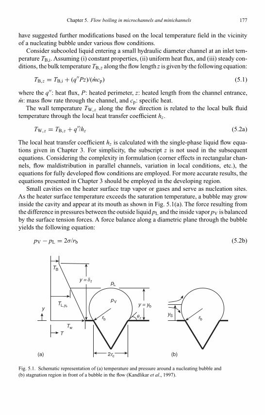
Kandlikar I044527-Ch05.tex 26/10/2005 18: 11 Page 177
Chapter 5. Flow boiling in microchannels and minichannels 177
have suggested further modifications based on the local temperature field in the vicinityof a nucleating bubble under various flow conditions.
Consider subcooled liquid entering a small hydraulic diameter channel at an inlet tem-perature TB,i. Assuming (i) constant properties, (ii) uniform heat flux, and (iii) steady con-ditions, the bulk temperature TB, z along the flow length z is given by the following equation:
TB, z = TB,i + (q′′Pz)/(mcp) (5.1)
where the q′′: heat flux, P: heated perimeter, z: heated length from the channel entrance,m: mass flow rate through the channel, and cp: specific heat.
The wall temperature TW, z along the flow direction is related to the local bulk fluidtemperature through the local heat transfer coefficient hz .
TW, z = TB, z + q′′/hz (5.2a)
The local heat transfer coefficient hz is calculated with the single-phase liquid flow equa-tions given in Chapter 3. For simplicity, the subscript z is not used in the subsequentequations. Considering the complexity in formulation (corner effects in rectangular chan-nels, flow maldistribution in parallel channels, variation in local conditions, etc.), theequations for fully developed flow conditions are employed. For more accurate results, theequations presented in Chapter 3 should be employed in the developing region.
Small cavities on the heater surface trap vapor or gases and serve as nucleation sites.As the heater surface temperature exceeds the saturation temperature, a bubble may growinside the cavity and appear at its mouth as shown in Fig. 5.1(a). The force resulting fromthe difference in pressures between the outside liquid pL and the inside vapor pV is balancedby the surface tension forces. A force balance along a diametric plane through the bubbleyields the following equation:
pV − pL = 2σ/rb (5.2b)
TB
TL,yb y = yb
2rc
pL
pV
y = dt
ur
y
T
ySrb rb
Tw
(a) (b)
Fig. 5.1. Schematic representation of (a) temperature and pressure around a nucleating bubble and(b) stagnation region in front of a bubble in the flow (Kandlikar et al., 1997).
Kandlikar I044527-Ch05.tex 26/10/2005 18: 11 Page 178
178 Heat transfer and fluid flow in minichannels and microchannels
where σ: surface tension, and rb: bubble radius. Whether the bubble is able to nucleateand the cavity is able to act as a nucleation site depends on the local temperature fieldaround the bubble. The local temperature in the liquid is evaluated by assuming a lineartemperature gradient in a liquid sublayer of thickness y = δt from the temperature at thewall to the temperature in the bulk liquid. Equating the heat transfer rates obtained fromthe equivalent conduction and convection equations, the thickness δt is given by:
δt = kL/h (5.3)
where kL is the thermal conductivity of the liquid and h is the single-phase heat transfercoefficient in the liquid prior to nucleation. The heat transfer coefficient can be obtainedfrom equations given in Chapter 3.
At a given location z, the temperature in the liquid at y = yb is obtained from the lineartemperature profile as shown in Fig. 5.1:
TL,yb = TW − (yb/δt)(TW − TB) (5.4)
where TL,yb : liquid temperature at y = yb, and TW: wall temperature. Neglecting theeffect of interface curvature on the change in saturation temperature, and introducingthe Clausius–Clapeyron equation, dp/dT = hLV/[TSat(vV − vL)], into Eq. (5.2b) to relatethe pressure difference to the corresponding difference in saturation temperatures, theexcess temperature needed to sustain a vapor bubble is given by:
(pV − pL) = [TL,Sat(pV) − TSat]hLV
TSat(vV − vL)(5.5)
where TL,Sat(pV): saturation temperature in K corresponding to the pressure pV, TSat:saturation temperature in K corresponding to the system pressure pL, hLV: latent heat ofvaporization at pL, and vV and vL: vapor and liquid specific volumes. Combining Eqs.(5.2a) and (5.5), and assuming vV >> vL, we get:
TL,Sat(pV) = TSat + 2σ
rb
TSat
ρVhLV(5.6)
As a condition for nucleation, the liquid temperature TL,yb in Eq. (5.4) should be greaterthan TL,Sat(pV), which represents the minimum temperature required at any point onthe liquid–vapor interface to sustain the vapor bubble as given by Eq. (5.6). CombiningEqs. (5.4) and (5.6) yields the condition for nucleating cavities of specific radii:
(yb/δt)(TW − TB) − (TW − TSat) + 2σ
rb
TSat
ρVhLV= 0 (5.7)
The liquid subcooling and wall superheat are defined as follows:
TSub = TSat − TB (5.8)
TSat = TW − TSat (5.9)

Kandlikar I044527-Ch05.tex 26/10/2005 18: 11 Page 179
Chapter 5. Flow boiling in microchannels and minichannels 179
The bubble radius rb and height yb are related to the cavity mouth radius rc through thereceding contact angle θr as follows:
rb = rc/sin θr (5.10)
yb = rb(1 + cos θr) = rc(1 + cos θr)/sin θr (5.11)
Substituting Eqs. (5.10) and (5.11) into Eq. (5.7), and solving the resulting quadratic equa-tion for rc, Davis and Anderson (1966) obtained the range of nucleation cavities given by:
{rc,min, rc,max} = δt sin θr
2(1 + cos θr)
(TSat
TSat +TSub
)
×(
1 ∓√
1 − 8σTSat(TSat +TSub)(1 + cos θr)
ρVhLVδtT 2Sat
)(5.12)
The minimum and maximum cavity radii rc,min and rc,max are obtained from the negativeand positive signs of the radical in Eq. (5.12), respectively.
Different investigators have used different models to relate the bubble radius to thecavity radius and to the location where the liquid temperature TL is determined. Hsu(1962) assumed yb = 1.6rb, which effectively translates into a receding contact angle ofθr = 53.1◦. Substituting this value into Eq. (5.12), the range of cavities nucleating fromHsu’s criterion is given by:
{rc,min, rc,max} = δt
4
(TSat
TSat +TSub
)
×(
1 ∓√
1 − 12.8σTSat(TSat +TSub)
ρVhLVδtT 2Sat
)(5.13)
Bergles and Rohsenow (1964), and Sato and Matsumura (1964) considered a hemisphericalbubble at the nucleation inception with yb = rb = rc. The resulting range of nucleatingcavities is given by:
{rc,min, rc,max} = δt
2
(TSat
TSat +TSub
)
×(
1 ∓√
1 − 8σTSat(TSat +TSub)
ρVhLVδtT 2Sat
)(5.14)
Kandlikar et al. (1997) analyzed the flow around a bubble and found that a stagnation pointoccurred at a certain distance yS from the bubble base as shown in Fig. 5.1(b). For recedingcontact angles in the range of 20–60◦, the location of the stagnation point was given by:
yS = 1.1rb = 1.1(rc/sin θr) (5.15)

Kandlikar I044527-Ch05.tex 26/10/2005 18: 11 Page 180
180 Heat transfer and fluid flow in minichannels and microchannels
Since a streamline farther away from the wall at this location would sweep over the bubbleas seen in Fig. 5.1(b), the temperature at y = yS was taken as the liquid temperature aty = yb. The resulting range of nucleation cavities is then given by:
{rc,min, rc,max} = δt sin θr
2.2
(TSat
TSat +TSub
)
×(
1 ∓√
1 − 8.8σTSat(TSat +TSub)
ρVhLVδtT 2Sat
)(5.16)
Note that there was a typographical error in the original publication by Kandlikar et al.(1997). The correct value for the constant is 8.8 as given in Eq. (5.16), though the actualgraphs in the original publication were plotted using the correct value of 8.8 by Kandlikaret al. (1997).
The onset of nucleate boiling (ONB) is of particular interest in flow boiling. The radiusrc,crit of the first cavity that will nucleate (if present) is obtained by setting the radical termin Eq. (5.16) to zero:
rc,crit = δt sin θr
2.2
(TSat
TSat +TSub
)(5.17)
For a given heat flux, the wall superheat at the ONB, TSat,ONB is given by:
TSat,ONB = √8.8σTSatq′′/(ρVhLVkL) (5.18)
If the local wall superheat at a given section is lower than that given by Eq. (5.18), nucleationwill not occur. The local subcooling at the ONB can be determined from the followingequation:
TSub,ONB = q′′
h−TSat,ONB (5.19)
In a channel with subcooled liquid entering, the local subcooling at the section where nucle-ation occurs is given by Eq. (5.19). If the subcooling is negative, it means that the local liq-uid is superheated and will cause extremely high bubble growth rates. Later it will be shownthat such high rates result in reverse flow that leads to severe pressure drop fluctuations.
Figure 5.2 shows the comparison of different nucleation models with the experimentaldata by Kandlikar et al. (1997). A high-power microscope and a high-speed camera wereused to visualize the nucleation activity and measure the underlying cavity dimensions.Cavities were largely rectangular in shape and the larger side of the opening was used indetermining the cavity radius. The cavities nucleate at a certain minimum wall superheatand continue to nucleate for higher wall superheats. A majority of the data points shown inFig. 5.2 correspond to higher values of wall superheat than the minimum required for nucle-ation. It is seen that all data points fall very close to or above the criterion given by Eq. (5.14).
As seen from Fig. 5.2, the criterion by Davis and Anderson predicts higher wall super-heats for larger cavities, whereas Bergles and Rohsenow’s criterion allows the larger cavities
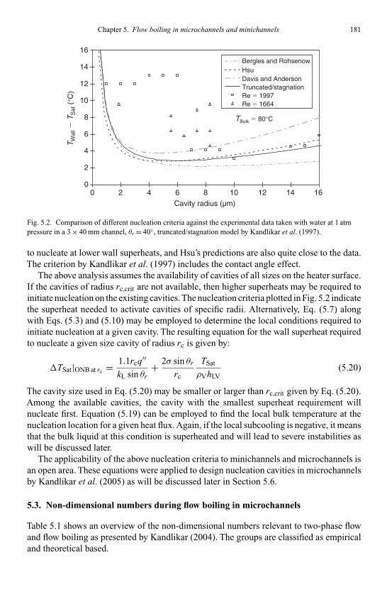
Kandlikar I044527-Ch05.tex 26/10/2005 18: 11 Page 181
Chapter 5. Flow boiling in microchannels and minichannels 181
0
2
4
6
8
10
12
14
16
0 2 4 6 8 10 12 14 16Cavity radius (µm)
TW
all �
TS
at (
°C)
Bergles and RohsenowHsuDavis and AndersonTruncated/stagnationRe � 1997Re � 1664
TBulk � 80°C
Fig. 5.2. Comparison of different nucleation criteria against the experimental data taken with water at 1 atmpressure in a 3 × 40 mm channel, θr = 40◦, truncated/stagnation model by Kandlikar et al. (1997).
to nucleate at lower wall superheats, and Hsu’s predictions are also quite close to the data.The criterion by Kandlikar et al. (1997) includes the contact angle effect.
The above analysis assumes the availability of cavities of all sizes on the heater surface.If the cavities of radius rc,crit are not available, then higher superheats may be required toinitiate nucleation on the existing cavities. The nucleation criteria plotted in Fig. 5.2 indicatethe superheat needed to activate cavities of specific radii. Alternatively, Eq. (5.7) alongwith Eqs. (5.3) and (5.10) may be employed to determine the local conditions required toinitiate nucleation at a given cavity. The resulting equation for the wall superheat requiredto nucleate a given size cavity of radius rc is given by:
TSat|ONB at rc = 1.1rcq′′
kL sin θr+ 2σ sin θr
rc
TSat
ρVhLV(5.20)
The cavity size used in Eq. (5.20) may be smaller or larger than rc,crit given by Eq. (5.20).Among the available cavities, the cavity with the smallest superheat requirement willnucleate first. Equation (5.19) can be employed to find the local bulk temperature at thenucleation location for a given heat flux. Again, if the local subcooling is negative, it meansthat the bulk liquid at this condition is superheated and will lead to severe instabilities aswill be discussed later.
The applicability of the above nucleation criteria to minichannels and microchannels isan open area. These equations were applied to design nucleation cavities in microchannelsby Kandlikar et al. (2005) as will be discussed later in Section 5.6.
5.3. Non-dimensional numbers during flow boiling in microchannels
Table 5.1 shows an overview of the non-dimensional numbers relevant to two-phase flowand flow boiling as presented by Kandlikar (2004). The groups are classified as empiricaland theoretical based.
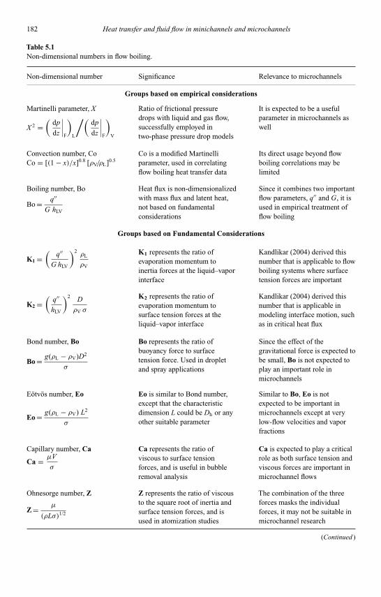
Kandlikar I044527-Ch05.tex 26/10/2005 18: 11 Page 182
182 Heat transfer and fluid flow in minichannels and microchannels
Table 5.1Non-dimensional numbers in flow boiling.
Non-dimensional number Significance Relevance to microchannels
Groups based on empirical considerations
Martinelli parameter, X Ratio of frictional pressure It is expected to be a usefuldrops with liquid and gas flow, parameter in microchannels assuccessfully employed in welltwo-phase pressure drop models
X 2 =(
dp
dz
∣∣∣∣F
)L
/(dp
dz
∣∣∣∣F
)V
Convection number, Co Co is a modified Martinelli Its direct usage beyond flowCo = [(1 − x)/x]0.8 [ρV/ρL]0.5 parameter, used in correlating boiling correlations may be
flow boiling heat transfer data limited
Boiling number, Bo Heat flux is non-dimensionalized Since it combines two importantwith mass flux and latent heat, flow parameters, q′′ and G, it isnot based on fundamental used in empirical treatment ofconsiderations flow boiling
Bo = q′′
G hLV
Groups based on Fundamental Considerations
K1 represents the ratio of Kandlikar (2004) derived thisevaporation momentum to number that is applicable to flowinertia forces at the liquid–vapor boiling systems where surfaceinterface tension forces are important
K1 =(
q′′
G hLV
)2ρL
ρV
K2 represents the ratio of Kandlikar (2004) derived thisevaporation momentum to number that is applicable insurface tension forces at the modeling interface motion, suchliquid–vapor interface as in critical heat flux
K2 =(
q′′
hLV
)2 D
ρV σ
Bond number, Bo Bo represents the ratio of Since the effect of thebuoyancy force to surface gravitational force is expected totension force. Used in droplet be small, Bo is not expected toand spray applications play an important role in
microchannels
Bo = g(ρL − ρV)D2
σ
Eötvös number, Eo Eo is similar to Bond number, Similar to Bo, Eo is notexcept that the characteristic expected to be important indimension L could be Dh or any microchannels except at veryother suitable parameter low-flow velocities and vapor
fractions
Eo = g(ρL − ρV) L2
σ
Capillary number, Ca Ca represents the ratio of Ca is expected to play a criticalviscous to surface tension role as both surface tension andforces, and is useful in bubble viscous forces are important inremoval analysis microchannel flows
Ca = µV
σ
Ohnesorge number, Z Z represents the ratio of viscous The combination of the threeto the square root of inertia and forces masks the individualsurface tension forces, and is forces, it may not be suitable inused in atomization studies microchannel research
Z = µ
(ρLσ)1/2
(Continued )

Kandlikar I044527-Ch05.tex 26/10/2005 18: 11 Page 183
Chapter 5. Flow boiling in microchannels and minichannels 183
Table 5.1(Continued)
Non-dimensional number Significance Relevance to microchannels
Weber number, We We represents the ratio of the We is useful in studying theinertia to the surface tension relative effects of surfaceforces. For flow in channels, Dh tension and inertia forces onis used in place of L flow patterns in microchannels
We = LG2
ρσ
Jakob number, Ja Ja represents the ratio of the Ja may be used in studyingsensible heat required for liquid superheat prior toreaching a saturation nucleation in microchannels andtemperature to the latent heat effect of subcooling
Ja = ρL
ρV
cp,L T
hLV
Adapted from Kandlikar (2004).
Vapor plugLiquid
Evaporation atthe interface
Flow
F �
Channel wall
M
F �S
Fig. 5.3. Schematic representation of evaporation momentum and surface tension forces on an evaporatinginterface in a microchannel or a minichannel (Kandlikar, 2004).
With the exception of the empirically derived Boiling number, the non-dimensionalnumbers used in flow boiling applications have not incorporated the effect of heat flux.This effect was recognized by Kandlikar (2004) as causing rapid interface movement duringthe highly efficient evaporation process occurring in microchannels. Figure 5.3 shows anevaporating interface occupying the entire channel. The change of phase from liquid tovapor is associated with a large momentum change due to the higher specific volume ofthe vapor phase. The resulting force is used in deriving two non-dimensional groups K1and K2 as shown in Table 5.1. The evaporation momentum force, the inertia force and thesurface tension forces are primarily responsible for the two-phase flow characteristics andthe interface shape and its motion during flow boiling in microchannels and minichannels.K1 represents a modified boiling number with the incorporation of the liquid to vapordensity ratio, while K2 relates the evaporation momentum and surface tension forces.Future research work in this area is needed to utilize these numbers in modeling of theflow patterns and critical heat flux (CHF) phenomenon.

Kandlikar I044527-Ch05.tex 26/10/2005 18: 11 Page 184
184 Heat transfer and fluid flow in minichannels and microchannels
The Bond number compares the surface tension forces and the gravitational forces.Under flow boiling conditions in narrow channels, the influence of gravity is expectedto be quite low. The Weber number and Capillary numbers account for the surface ten-sion, inertia, and viscous forces. These numbers are expected to be useful parameters inrepresenting some of the complex features of the flow boiling phenomena.
5.4. Flow patterns, instabilities and heat transfer mechanisms during flowboiling in minichannels and microchannels
A number of investigators have studied the flow patterns, and pressure drop and heattransfer characteristics of flow boiling in minichannels and microchannels. Kandlikar(2002a) presented a comprehensive summary in a tabular form. An abridged version of thetable is reproduced in Table 5.2. The ranges of parameters investigated along with somekey results are included in this table. Some of the researchers focused on obtaining theheat transfer coefficient data. Table 5.3, derived from Steinke and Kandlikar (2004), givesthe details of the experimental conditions of some of the studies reported in the literature.It may be noted that there are very few local data available that report local heat transfercoefficients.
The influence of surface tension forces becomes more dominant in small diameterchannels, and this is reflected in the flow patterns observed in these channels. A compre-hensive summary of adiabatic flow pattern studies is presented by Hewitt (2000). Kandlikar(2002a, b) presented an extensive summary of flow patterns and associated heat transferduring flow boiling in microchannels and minichannels. Although a number of inves-tigators have conducted extensive studies on adiabatic two-phase flows with air–watermixtures, there are relatively fewer studies available on evaporating flows. Cornwell andKew (1992) conducted experiments with R-113 flowing in 1.2 mm × 0.9 mm rectangularchannels. They mainly observed three flow patterns as shown in Fig. 5.4 (isolated bubbles,confined bubbles and high quality annular flow). They noted the heat transfer to be stronglyinfluenced by the heat flux, indicating the dominance of nucleate boiling in the isolatedbubble region. The convective effects became important during other flow patterns. Theseflow patterns are observed in minichannels at relatively low heat flux conditions.
Mertz et al. (1996) conducted experiments in single and multiple channels with waterand R-141b boiling in rectangular channels 1, 2, and 3 mm wide. They observed thepresence of nucleate boiling, confined bubble flow and annular flow. The bubble generationprocess was not a continuous process, and large pressure fluctuations were observed. Kaszaet al. (1997) observed the presence of nucleate boiling on the channel wall similar to thepool boiling case. They also observed nucleation in the thin films surrounding a vapor core.
Bonjour and Lallemand (1998) reported flow patterns of R-113 boiling in a narrow spacebetween two vertical surfaces. They noted that the Bond number effectively identifies thetransition of flow patterns from conventional diameter tubes to minichannels. For smallerdiameter channels, however, the gravitational forces become less important and Bondnumber is not useful in modeling the flow characteristics. The presence of nucleationfollowed by bubble growth was visually observed by Kandlikar and Stumm (1995), andKandlikar and Spiesman (1997).

Kandlikar I044527-Ch05.tex 26/10/2005 18: 11 Page 185
Chapter 5. Flow boiling in microchannels and minichannels 185
Table 5.2Summary of investigations on evaporation in minichannels and Microchannels.
Fluid andranges of Channel size, Dh
parameters (mm) horizontalG(kg/m2-s), (unless
Author (year) q′′-(kW/m2) otherwise stated) Flow patterns Remarks
Lazarek and R-113, Circular, Not observed Subcooled and saturatedBlack (1982) G = 125–750. D = 3.1, L = 123 data, h almost constant
q′′ = 14–380 and 246 in the two-phase region,dependent on q′′. Behaviorsimilar to large diametertubes
Cornwell and R-113, Rectangular, Isolated bubble, h was dependent on theKew (1992) G = 124–627, 75 channel confined bubble, flow pattern. Isolated
q′′ = 3–33 1.2 × 0.9 annular slug bubble region, h ∼ q0.7,36 channel lower q effect in confined3.25 × 1.1 bubble region, convection
dominant in annular slugregion
Moriyama and R-113, Rectangular, Flattened bubbles, Data in narrow gapsInoue (1992) G = 200–1000, 0.035–0.11 gap, with coalescence, obtained and correlated
q′′ = 4–30 w= 30, L = 265 liquid strips/film with an annular film flowmodel. Nucleate boilingignored, although h variedwith q
Wambsganss R-113 Circular, Not reported Except at the lowest heatet al. (1993) G = 50–100, D = 2.92 mm and mass fluxes, both
q′′ = 8.8–90.7 nucleate boiling andconvective boilingcomponents were present
Bowers and R-113, Minichannels and, Not studied Minichannels and micro-Mudawar (1994) 0.28–1.1 ml/s, microchannels channels compared. Mini-
q′′ = 1000–2000 D = 2.54 and 0.51 channels are preferableunless liquid inventory orweight constraints aresevere
Mertz Water/R-141b Rectangular, Nucleate boiling, Single- and multi-channelet al. (1996) G = 50–300 1, 2, and 3 mm confined bubble test sections. Flow boiling
q′′ = 3–227 wide, aspect and annular pulsations in multi-ratio up to 3 channels, reverse flow,
nucleate boiling dominant
Ravigururajan R-124, 270 µm wide, Not studied Experiments wereet al. (1996) 0.6–5 ml/s, 1 mm deep, and conducted over 0–0.9
20–400 W 20.52 mm long, quality and 5◦C inletsubcooling. Wall superheatfrom 0◦C to 80◦C
(Continued )
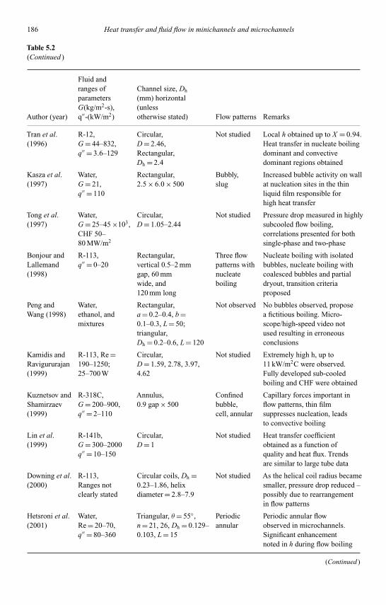
Kandlikar I044527-Ch05.tex 26/10/2005 18: 11 Page 186
186 Heat transfer and fluid flow in minichannels and microchannels
Table 5.2(Continued )
Fluid andranges of Channel size, Dh
parameters (mm) horizontalG(kg/m2-s), (unless
Author (year) q′′-(kW/m2) otherwise stated) Flow patterns Remarks
Tran et al. R-12, Circular, Not studied Local h obtained up to X = 0.94.(1996) G = 44–832, D = 2.46, Heat transfer in nucleate boiling
q′′ = 3.6–129 Rectangular, dominant and convectiveDh = 2.4 dominant regions obtained
Kasza et al. Water, Rectangular, Bubbly, Increased bubble activity on wall(1997) G = 21, 2.5 × 6.0 × 500 slug at nucleation sites in the thin
q′′ = 110 liquid film responsible forhigh heat transfer
Tong et al. Water, Circular, Not studied Pressure drop measured in highly(1997) G = 25–45 ×103, D = 1.05–2.44 subcooled flow boiling,
CHF 50– correlations presented for both80 MW/m2 single-phase and two-phase
Bonjour and R-113, Rectangular, Three flow Nucleate boiling with isolatedLallemand q′′ = 0–20 vertical 0.5–2 mm patterns with bubbles, nucleate boiling with(1998) gap, 60 mm nucleate coalesced bubbles and partial
wide, and boiling dryout, transition criteria120 mm long proposed
Peng and Water, Rectangular, Not observed No bubbles observed, proposeWang (1998) ethanol, and a = 0.2–0.4, b = a fictitious boiling. Micro-
mixtures 0.1–0.3, L = 50; scope/high-speed video nottriangular, used resulting in erroneousDh = 0.2–0.6, L = 120 conclusions
Kamidis and R-113, Re = Circular, Not studied Extremely high h, up toRavigururajan 190–1250; D = 1.59, 2.78, 3.97, 11 kW/m2C were observed.(1999) 25–700 W 4.62 Fully developed sub-cooled
boiling and CHF were obtained
Kuznetsov and R-318C, Annulus, Confined Capillary forces important inShamirzaev G = 200–900, 0.9 gap × 500 bubble, flow patterns, thin film(1999) q′′ = 2–110 cell, annular suppresses nucleation, leads
to convective boiling
Lin et al. R-141b, Circular, Not studied Heat transfer coefficient(1999) G = 300–2000 D = 1 obtained as a function of
q′′ = 10–150 quality and heat flux. Trendsare similar to large tube data
Downing et al. R-113, Circular coils, Dh = Not studied As the helical coil radius became(2000) Ranges not 0.23–1.86, helix smaller, pressure drop reduced –
clearly stated diameter = 2.8–7.9 possibly due to rearrangementin flow patterns
Hetsroni et al. Water, Triangular, θ= 55◦, Periodic Periodic annular flow(2001) Re = 20–70, n = 21, 26, Dh = 0.129– annular observed in microchannels.
q′′ = 80–360 0.103, L = 15 Significant enhancementnoted in h during flow boiling
(Continued )
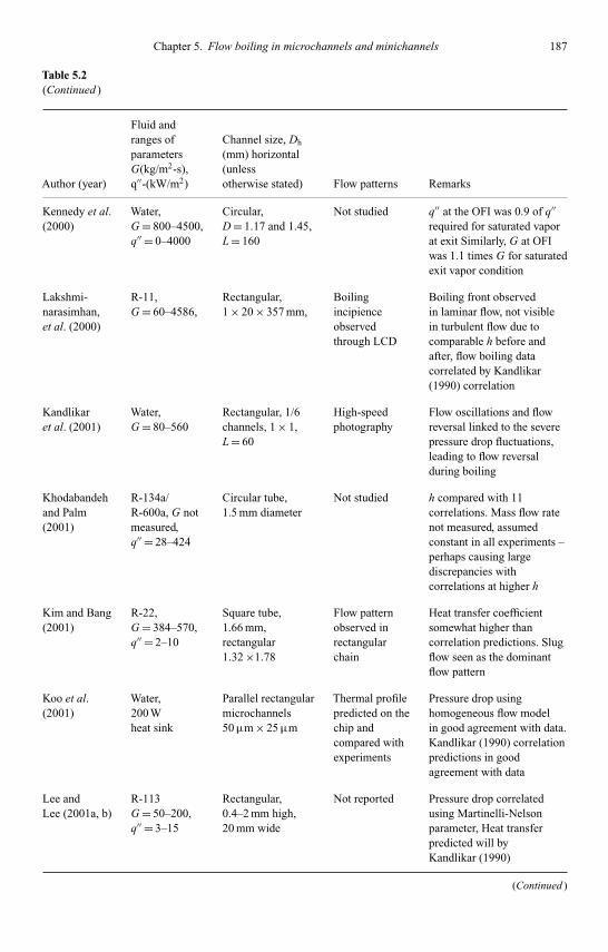
Kandlikar I044527-Ch05.tex 26/10/2005 18: 11 Page 187
Chapter 5. Flow boiling in microchannels and minichannels 187
Table 5.2(Continued )
Fluid andranges of Channel size, Dh
parameters (mm) horizontalG(kg/m2-s), (unless
Author (year) q′′-(kW/m2) otherwise stated) Flow patterns Remarks
Kennedy et al. Water, Circular, Not studied q′′ at the OFI was 0.9 of q′′(2000) G = 800–4500, D = 1.17 and 1.45, required for saturated vapor
q′′ = 0–4000 L = 160 at exit Similarly, G at OFIwas 1.1 times G for saturatedexit vapor condition
Lakshmi- R-11, Rectangular, Boiling Boiling front observednarasimhan, G = 60–4586, 1 × 20 × 357 mm, incipience in laminar flow, not visibleet al. (2000) observed in turbulent flow due to
through LCD comparable h before andafter, flow boiling datacorrelated by Kandlikar(1990) correlation
Kandlikar Water, Rectangular, 1/6 High-speed Flow oscillations and flowet al. (2001) G = 80–560 channels, 1 × 1, photography reversal linked to the severe
L = 60 pressure drop fluctuations,leading to flow reversalduring boiling
Khodabandeh R-134a/ Circular tube, Not studied h compared with 11and Palm R-600a, G not 1.5 mm diameter correlations. Mass flow rate(2001) measured, not measured, assumed
q′′ = 28–424 constant in all experiments –perhaps causing largediscrepancies withcorrelations at higher h
Kim and Bang R-22, Square tube, Flow pattern Heat transfer coefficient(2001) G = 384–570, 1.66 mm, observed in somewhat higher than
q′′ = 2–10 rectangular rectangular correlation predictions. Slug1.32 ×1.78 chain flow seen as the dominant
flow pattern
Koo et al. Water, Parallel rectangular Thermal profile Pressure drop using(2001) 200 W microchannels predicted on the homogeneous flow model
heat sink 50 µm × 25 µm chip and in good agreement with data.compared with Kandlikar (1990) correlationexperiments predictions in good
agreement with data
Lee and R-113 Rectangular, Not reported Pressure drop correlatedLee (2001a, b) G = 50–200, 0.4–2 mm high, using Martinelli-Nelson
q′′ = 3–15 20 mm wide parameter, Heat transferpredicted will byKandlikar (1990)
(Continued )

Kandlikar I044527-Ch05.tex 26/10/2005 18: 11 Page 188
188 Heat transfer and fluid flow in minichannels and microchannels
Table 5.2(Continued)
Fluid andranges of Channel size, Dh
parameters (mm) horizontalG(kg/m2-s), (unless
Author (year) q′′-(kW/m2) otherwise stated) Flow patterns Remarks
correlation for film Re> 200,new correlation developedusing film flow model forfilm Re< 200
Serizawa and Air–water, Circular tubes, Flow patterns Two new flow patternsFeng (2001) jL = 0.003– diameters of identified over identified: liquid ring flow
17.52 m/s, 50 µm for the ranges of and liquid lump flow. Steam–jG = 0.0012– air–water and of flow rates water ranges not given295.3 m/s. and 25 µm studied
for steam–water
Warrier et al. FC-84, Rectangular, Not studied Overall pressure drop and(2001) G = 557–1600, dimensions not local heat transfer coefficient
q′′ = 59.9 available, hydraulic determined. A constant valuediameter = 0.75 mm of C = 38 used in Eq. (1).
Heat transfer coefficientcorrelated as a functionof Boiling number alone
OFI: Onset of flow instability.Adapted from Kandlikar (2002a).
Table 5.3Available literature for evaporation of pure liquid flows in parallel minichannel and microchannel passages.
Author (year) Fluid Dh (mm) Re G (kg/m2s) (kW/m2) Type* Vis.**
Lazarek and Black (1982) R-113 3.150 57–340 125–750 14–380 O NMoriyama and Inoue (1992) R-113 0.140–0.438 107–854 200–1000 4.0–30 O/L YWambsganss et al. (1993) R-113 2.920 313–2906 50–300 8.8–90.75 L NBowers and Mudawar (1994) R-113 2.540 and 14–1714 20–500 30–2000 O N
0.510Peng et al. (1994) Water 0.133–0.343 200–2000 500–1626 – O NCuta et al. (1996) R-124 0.850 100–570 32–184 1.0–400 O NMertz et al. (1996) Water 3.100 57–210 50–300 10–110 O NRavigururajan et al. (1996) R-124 0.425 217–626 142–411 5.0–25 L NTran et al. (1996) R-12 2.400–2.460 345–2906 44–832 3.6–129 L NKew and Cornwell (1997) R-141b 1.390–3.690 1373–5236 188–1480 9.7–90 L YRavigururajan (1998) R-124 0.850 11,115– 3583–10,369 20–700 L N
32,167Yan and Lin (1998) R-134a 2.000 506–2025 50–900 5.0–20 L NKamidis and R-113 1.540–4.620 190–1250 90–200 50–300 L NRavigururajan (1999)
(Continued )

Kandlikar I044527-Ch05.tex 26/10/2005 18: 11 Page 189
Chapter 5. Flow boiling in microchannels and minichannels 189
Table 5.3(Continued)
Author (year) Fluid Dh (mm) Re G (kg/m2s) (kW/m2) Type* Vis.**
Lin et al. (1999) R-141b 1.100 1591 568 – L NMudawar and Bowers Water 0.902 16–49 2 × 10⁴– 1 × 10³– O N
(1999) 1 × 10⁵ 2 × 10⁵
Bao et al. (2000) R-11/R-123 1.950 1200–4229 50–1800 5–200 L NLakshminarasimhan et al. R-11 3.810 1311– 60–4586 7.34–37.9 O Y
(2000) 11,227Jiang et al. (2001) Water 0.026 1541–4811 2 × 10⁴– – O Y
5 × 10⁴
Kandlikar et al. (2001) Water 1.000 100–556 28–48 1–150 O YKim and Bang (2001) R-22 1.660 1883–2796 384–570 2.0–10 L YKoizumi et al. (2001) R-113 0.500–5.000 67–5398 100–800 1.0–110 O YLee and Lee (2001c) R-113 1.569–7.273 220–1786 52–209 2.98–15.77 L NLin et al. (2001) R-141b 1.100 536–2955 50–3500 1–300 L NHetsroni et al. (2002) Vertrel XF 0.158 35–68 148–290 22.6–36 L YQu and Mudawar (2002) Water 0.698 338–1001 135–402 1–1750 N NWarrier et al. (2002) FC-84 0.750 440–1552 557–1600 1.0–50 L NYen et al. (2002) R-123 0.190 65–355 50–300 5.46–26.9 L YYu et al. (2002) Water 2.980 534–1612 50–200 50–200 L NZhang et al. (2002) Water 0.060 127 590 2.2 ×10⁴ O NFaulkner and Shekarriz Water 1.846–3.428 20,551– 3106–6225 250–2750 O N
(2003) 41,188Hetsroni et al. (2003) Water 0.103–0.161 8.0–42 51–500 80–220 O YKuznetsov et al. (2003) R-21 1.810 148–247 30–50 3.0–25 L NLee et al. (2003) Water 0.036–0.041 22–51 170–341 0.2–301 O YLee and Garimella (2003) Water 0.318–0.903 300–3500 260–1080 – O NMolki et al. (2003) R-134a 1.930 717–1614 100–225 14 L NPark et al. (2003) R-22 1.660 1473–2947 300–600 10.0–20 L NQu and Mudawar (2003) Water 0.349 338–1001 135–402 10.0–1300 L NWu and Cheng (2003) Water 0.186 75–97 112 226 O YSteinke and Water 0.207 116–1218 157–1782 5–930 L Y
Kandlikar (2004)
Adapted from Steinke and Kandlikar (2004).* O = overall, L = local; **Visualization, Y = yes, N = no.
Isolated bubble Confined bubble
Low x High x
Fig. 5.4. Flow patterns observed by Cornwell and Kew (1992) during flow boiling of R-113 in1.2 mm × 0.9 mm rectangular channel.
The contribution of nucleate boiling to flow boiling heat transfer was clearly confirmedin the above studies, as well as a number of other studies reported in the literature, (e.g.Lazarek and Black, 1982; Wambsganss et al., 1993; Tran et al., 1996; Yan and Lin,1998; Bao et al., 2000; Steinke and Kandlikar, 2004). However, for microchannels, it was

Kandlikar I044527-Ch05.tex 26/10/2005 18: 11 Page 190
190 Heat transfer and fluid flow in minichannels and microchannels
(a) (b)
Fig. 5.5. Flow patterns in 200 µm × 1054 µm parallel channels (a) expanding bubble flow pattern (Kandlikaret al., 2005) each frame shows the progression of boiling in the same channel at 1 ms time intervals, and(b) a snapshot of interface movements in six parallel channels connected by common headers (Kandlikar andBalasubramanian, 2005).
also noted that the rapid evaporation and growth of a vapor bubble following nucleationcaused major flow excursions, often resulting in reversed flow. Figure 5.5(a) shows asequence of frames obtained by Kandlikar et al. (2005) for water boiling in 200 µm squareparallel channels. The images are taken at intervals of 1 ms and the flow direction isupward. The growth of bubbles and their expansion against the flow direction is clearlyseen. Figure 5.5(b) shows the movement of the liquid–vapor interface in both directionsas obtained by Kandlikar and Balasubramanian (2005). Similar observations have beenmade by a number of investigators, including Mertz et al. (1996), Kennedy et al. (2000),Kandlikar et al. (2001), Peles et al. (2001), Kandlikar (2002a, b), Zhang et al. (2002),Hetsroni et al. (2001; 2003), Peles (2003), Brutin andTadrist (2003), Steinke and Kandlikar(2004), and Balasubramanian and Kandlikar (2005).
Flow instability poses a major concern for flow boiling in minichannels and microchan-nels. A detailed description of the flow boiling instabilities is provided by Kandlikar (2002a,b; 2005). Instabilities during flow boiling have been studied extensively in large diametertubes. The excursive or Ledinegg and the parallel channel instabilities have been studiedextensively in the literature. These instabilities are also present in small diameter channelsas discussed by Bergles and Kandlikar (2005). Nucleation followed by an increase in theflow resistance due to two-phase flow in channels leads to a minimum in the pressuredrop demand curve leading to instabilities. Parallel channel instabilities also occur at theminimum in the pressure drop demand curve. In a microchannel, in addition to these twoinstabilities, there is a phenomenon that comes into play due to rapid bubble growth ratesthat causes instability and significant flow reversal problems. Large pressure fluctuationsat high frequencies have been reported by a number of investigators including Kew andCornwell (1996), Peles (2003), and Balasubramanian and Kandlikar (2005) among others.
The stability of the flow boiling process has been studied analytically using linear andnon-linear stability analyses. Some of the semi-empirical methods have yielded limitedsuccess (e.g. Peles et al., 2001; Brutin et al., 2002; Stoddard et al., 2002; Brutin and

Kandlikar I044527-Ch05.tex 26/10/2005 18: 11 Page 191
Chapter 5. Flow boiling in microchannels and minichannels 191
0123456789
10
0 1 2 3 4 5 6 7 8 9 10
Time (s)
Pre
ssur
e dr
op (
kPa)
Fig. 5.6. Pressure fluctuations observed during flow boiling of water in 1054 µm × 197 µm parallelminichannels (Balasubramanian and Kandlikar, 2005).
0
0.5
1
1.5
2
2.5
3
3.5
0 1 2 3 4
Length of bubble/slug (mm)
Bub
ble/
slug
gro
wth
rat
e (m
/s)
Fig. 5.7. Bubble/slug growth rates during flow boiling of water in 1054 µm × 197 µm parallel minichannels(Balasubramanian and Kandlikar, 2005).
Tadrist, 2003). However, these models cannot be tested because of a lack of extensiveexperimental data under stable boiling conditions. It is expected that with the availabilityof such data sets, more rigorous models, similar to those available for flow boiling inconventional sized tubes, will be developed in the near future.
The pressure fluctuations associated with the flow boiling process were observed bymany researchers as described earlier. Figure 5.6 shows a typical plot of the pressuredrop fluctuations obtained during flow boiling in minichannels by Balasubramanian andKandlikar (2005). A fast fourier transform analysis of the instantaneous pressure dropsignal revealed that the dominant frequency was dependent on the wall temperature andwas related to the nucleation activity within the channels. The growth rate of the growingbubbles was measured to be as high as 3.5 m/s. Figure 5.7 shows the growth rate of a slug in1054 µm × 197 µm parallel channels. As the bubbles reach the opposite channel wall, thegrowth rate stabilizes until the rapid evaporation from the walls causes the growth rate to

Kandlikar I044527-Ch05.tex 26/10/2005 18: 11 Page 192
192 Heat transfer and fluid flow in minichannels and microchannels
(1)
(2a)
(2b)
(2c)
Fig. 5.8. Schematic representation of bubble growth in (1) large diameter tubes, and (2a–c) microchannels andminichannels.
Expanding-bubble flow pattern in microchannel
Annular flow pattern in macrochannels
Evaporatingliquid filmLiquid slug
Vapor core
Flowing and evaporatingliquid film
Fig. 5.9. Comparison of the annular flow pattern in macrochannels and the expanding-bubble flow pattern inmicrochannels and minichannels.
increase again. The numerical simulation by Mukherjee and Kandlikar (2004) confirmedthe bubble growth observed in Fig. 5.7. Nucleation followed by rapid bubble growth isbelieved to be the cause of instabilities.
As a bubble grows under pool boiling conditions, the bubble growth rate is much higherimmediately following its inception. The growth rate is initially proportional to time t andis controlled by the inertial forces. As the bubble grows, the growth rate slows downand follows a t1/2 trend in the thermally controlled region. In large diameter channels(above 1–3 mm, depending on heat flux), the bubbles grow to sizes that are smaller thanthe channel diameter and leave the heater surface under inertia forces. In flow boiling inmacrochannels, the bubble growth is similar to that in pool boiling, except that the flowcauses the bubbles to depart early as shown in Fig. 5.8. These departing bubbles contributeto the bubbly flow. As more bubbles are formed, they coalesce and develop into slug andannular flows as shown in Fig. 5.9.

Kandlikar I044527-Ch05.tex 26/10/2005 18: 11 Page 193
Chapter 5. Flow boiling in microchannels and minichannels 193
(a)
(b)
(c)
(d)
(e)
(f)
Fig. 5.10. The expanding-bubble flow pattern observed in a 197 µm × 1054 µm channel, using water atatmospheric pressure, the time duration between successive images is 0.16 ms, G = 120 kg/m2 s,q′′ = 317 kW/m2, Ts = 110.9◦C, flow is from left to right (Kandlikar and Balasubramanian, 2005).
In microchannels and minichannels, as a bubble nucleates and initially grows in theinertia controlled region, it encounters the channel walls prior to entering the thermallycontrolled region found in the conventional channels. The large surface area to fluid volumeratio in the channel causes the liquid to heat up rapidly. Thus, the bubble encounters asuperheated liquid as it continues to grow and spreads over the other areas of the channelwall. The availability of heat from the superheated layer and from the channel walls causesa rapid expansion of the bubble, leading to the expanding-bubble flow pattern shown inFig. 5.8. The bubble occupies the entire channel cross-section and continues to grow asshown in Fig. 5.9. The expanding-bubble flow pattern differs from the annular flow patternmainly in that the liquid on the wall acts similar to the film under a growing vapor bubble,rather than as a flowing film. This makes the heat transfer mechanism very similar to thenucleate boiling mechanism. A number of investigators have confirmed the strong heat fluxdependence of the heat transfer coefficient during flow boiling in microchannels, whichindicates the dominance of nucleate boiling.
Figure 5.10 shows the expanding-bubble flow pattern observed during flow boilingin a rectangular minichannel by Kandlikar and Balasubramanian (2005). Note the rapidinterface movement on the right side of the bubbles (downstream). The liquid film isessentially stationary and occasionally dries out before the upstream liquid slug flowsthrough and rewets the surface. At other times, severe flow reversal was observed at thesame site, and the bubble interface moved upstream rapidly.
Mukherjee and Kandlikar (2004) performed a numerical simulation of the bubblegrowth process in a microchannel evaporator. The bubble initially nucleated from one ofthe walls and then grew to occupy the entire channel cross-section. The bubble shapes werecompared with the experimental observations by Balasubramanian and Kandlikar (2005)for the same geometry of 197 µm × 1054 µm with water in the expanding-bubble flowpattern region (Fig. 5.11). Their agreement validates numerical simulation as a powerfultool for analyzing the flow boiling phenomenon.
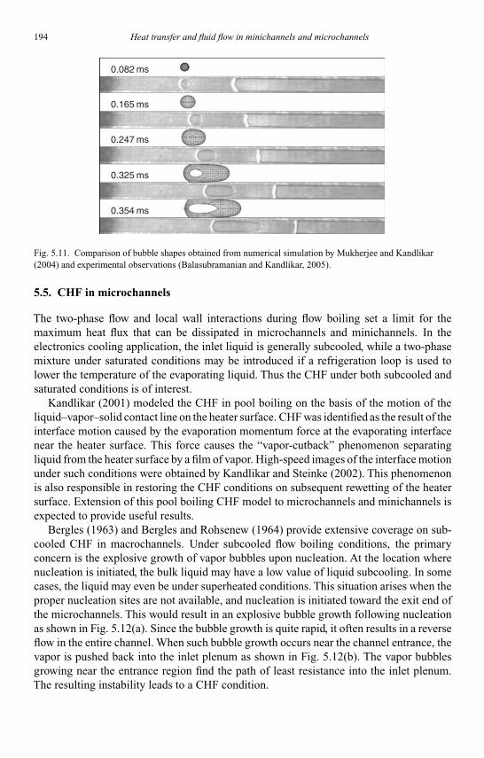
Kandlikar I044527-Ch05.tex 26/10/2005 18: 11 Page 194
194 Heat transfer and fluid flow in minichannels and microchannels
0.082 ms
0.165 ms
0.247 ms
0.325 ms
0.354 ms
Fig. 5.11. Comparison of bubble shapes obtained from numerical simulation by Mukherjee and Kandlikar(2004) and experimental observations (Balasubramanian and Kandlikar, 2005).
5.5. CHF in microchannels
The two-phase flow and local wall interactions during flow boiling set a limit for themaximum heat flux that can be dissipated in microchannels and minichannels. In theelectronics cooling application, the inlet liquid is generally subcooled, while a two-phasemixture under saturated conditions may be introduced if a refrigeration loop is used tolower the temperature of the evaporating liquid. Thus the CHF under both subcooled andsaturated conditions is of interest.
Kandlikar (2001) modeled the CHF in pool boiling on the basis of the motion of theliquid–vapor–solid contact line on the heater surface. CHF was identified as the result of theinterface motion caused by the evaporation momentum force at the evaporating interfacenear the heater surface. This force causes the “vapor-cutback” phenomenon separatingliquid from the heater surface by a film of vapor. High-speed images of the interface motionunder such conditions were obtained by Kandlikar and Steinke (2002). This phenomenonis also responsible in restoring the CHF conditions on subsequent rewetting of the heatersurface. Extension of this pool boiling CHF model to microchannels and minichannels isexpected to provide useful results.
Bergles (1963) and Bergles and Rohsenew (1964) provide extensive coverage on sub-cooled CHF in macrochannels. Under subcooled flow boiling conditions, the primaryconcern is the explosive growth of vapor bubbles upon nucleation. At the location wherenucleation is initiated, the bulk liquid may have a low value of liquid subcooling. In somecases, the liquid may even be under superheated conditions. This situation arises when theproper nucleation sites are not available, and nucleation is initiated toward the exit end ofthe microchannels. This would result in an explosive bubble growth following nucleationas shown in Fig. 5.12(a). Since the bubble growth is quite rapid, it often results in a reverseflow in the entire channel. When such bubble growth occurs near the channel entrance, thevapor is pushed back into the inlet plenum as shown in Fig. 5.12(b). The vapor bubblesgrowing near the entrance region find the path of least resistance into the inlet plenum.The resulting instability leads to a CHF condition.
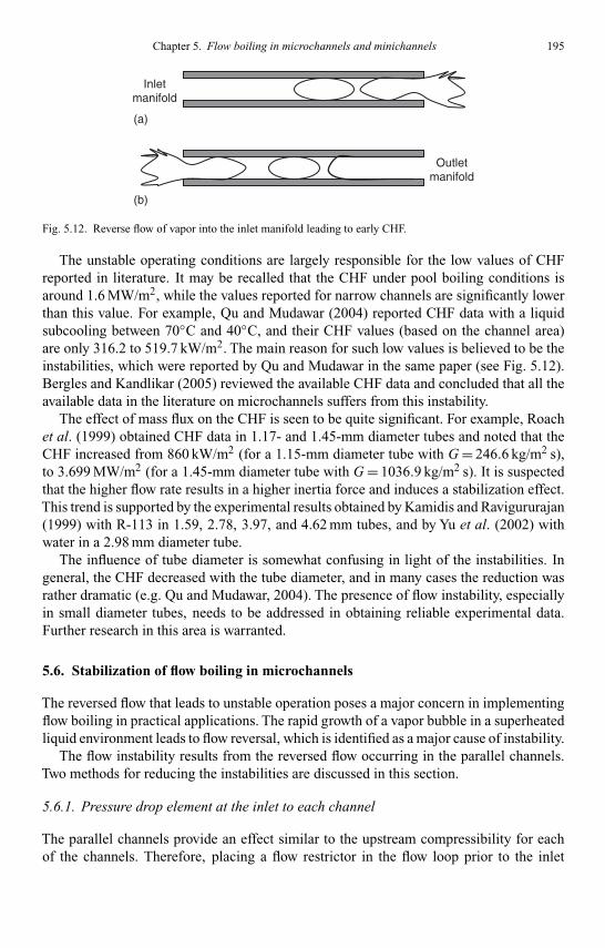
Kandlikar I044527-Ch05.tex 26/10/2005 18: 11 Page 195
Chapter 5. Flow boiling in microchannels and minichannels 195
Inletmanifold
Outletmanifold
(a)
(b)
Fig. 5.12. Reverse flow of vapor into the inlet manifold leading to early CHF.
The unstable operating conditions are largely responsible for the low values of CHFreported in literature. It may be recalled that the CHF under pool boiling conditions isaround 1.6 MW/m2, while the values reported for narrow channels are significantly lowerthan this value. For example, Qu and Mudawar (2004) reported CHF data with a liquidsubcooling between 70◦C and 40◦C, and their CHF values (based on the channel area)are only 316.2 to 519.7 kW/m2. The main reason for such low values is believed to be theinstabilities, which were reported by Qu and Mudawar in the same paper (see Fig. 5.12).Bergles and Kandlikar (2005) reviewed the available CHF data and concluded that all theavailable data in the literature on microchannels suffers from this instability.
The effect of mass flux on the CHF is seen to be quite significant. For example, Roachet al. (1999) obtained CHF data in 1.17- and 1.45-mm diameter tubes and noted that theCHF increased from 860 kW/m2 (for a 1.15-mm diameter tube with G = 246.6 kg/m2 s),to 3.699 MW/m2 (for a 1.45-mm diameter tube with G = 1036.9 kg/m2 s). It is suspectedthat the higher flow rate results in a higher inertia force and induces a stabilization effect.This trend is supported by the experimental results obtained by Kamidis and Ravigururajan(1999) with R-113 in 1.59, 2.78, 3.97, and 4.62 mm tubes, and by Yu et al. (2002) withwater in a 2.98 mm diameter tube.
The influence of tube diameter is somewhat confusing in light of the instabilities. Ingeneral, the CHF decreased with the tube diameter, and in many cases the reduction wasrather dramatic (e.g. Qu and Mudawar, 2004). The presence of flow instability, especiallyin small diameter tubes, needs to be addressed in obtaining reliable experimental data.Further research in this area is warranted.
5.6. Stabilization of flow boiling in microchannels
The reversed flow that leads to unstable operation poses a major concern in implementingflow boiling in practical applications. The rapid growth of a vapor bubble in a superheatedliquid environment leads to flow reversal, which is identified as a major cause of instability.
The flow instability results from the reversed flow occurring in the parallel channels.Two methods for reducing the instabilities are discussed in this section.
5.6.1. Pressure drop element at the inlet to each channel
The parallel channels provide an effect similar to the upstream compressibility for eachof the channels. Therefore, placing a flow restrictor in the flow loop prior to the inlet

Kandlikar I044527-Ch05.tex 26/10/2005 18: 11 Page 196
196 Heat transfer and fluid flow in minichannels and microchannels
X01
23
4
Y
0
0.25
0.5
0.75
1
Z
�0.5�0.25
00.25
0.5
0.00 ms
X01
23
4
Y
0
0.25
0.5
0.75
1
Z
�0.5�0.25
00.25
0.5
0.05 ms
X01
23
4
Y
0
0.25
0.5
0.75
1
Z
�0.5�0.25
00.25
0.5
0.11 ms
X01
23
4
Y
0
0.25
0.5
0.75
1
Z
�0.5�0.25
00.25
0.5
0.16 ms
X01
23
4
Y
0
0.25
0.5
0.75
1
Z
�0.5�0.25
00.25
0.5
0.22 ms
X01
23
4
Y
0
0.25
0.5
0.75
1Z
�0.5�0.25
00.25
0.5
0.29 ms
Fig. 5.13. Simulation of bubble growth in a microchannel with upstream to downstream flow resistance ratio,R = 1 (Mukherjee and Kandlikar, 2005).
manifold will not reduce the instability arising in each channel. To reduce the intensityand occurrence of reverse flow, a pressure drop element (essentially a flow constrictor ora length of reduced cross-sectional area) is placed at the entrance of each channel. Thisintroduces an added resistance to fluid flow, but provides an effective way to reduce theflow instabilities arising from the reverse flow.
Mukherjee and Kandlikar (2004; 2005) conducted an extensive numerical analysisof bubble growth in a microchannel in an effort to study the effect of the pressure dropelements on flow stabilization. They utilized the level set method to define the interface andtrack its movement by applying conservation equations. Figure 5.13 shows the consecutiveframes of a bubble growing in a microchannel. The resistance to flow in both the upstreamand downstream directions was the same. The bubble growth is seen to be slow at thebeginning, but becomes more rapid after the bubble touches the other heated channelwalls. This leads to an extension of the inertia-controlled region, where the heat transferis more efficient since it does not depend on the diffusion of heat across a thin layersurrounding the liquid–vapor interface.
Mukherjee and Kandlikar (2005) introduced a new parameter R to represent theupstream to downstream flow resistance ratio. In their simulation, they showed thatincreasing the upstream resistance reduced the intensity of the backflow. The results areshown in Fig. 5.14. In Fig. 5.14(a), the resistance in both directions is the same, whilein Fig. 5.14(b), the inlet to outlet ratio is 0.25 indicating a four-fold higher flow resis-tance in the backward direction. The resulting bubble growth in Fig. 5.14(b) shows thatreverse flow is completely eliminated in this case. As expected, the backflow characteris-tics were also found to be dependent on the heat flux and the local liquid superheat at thenucleation site.
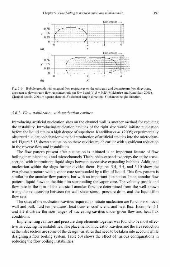
Kandlikar I044527-Ch05.tex 26/10/2005 18: 11 Page 197
Chapter 5. Flow boiling in microchannels and minichannels 197
X
0 1 2 3 4
X
0 1 2 3 4
0
0.25
0.5
0.75
1
Y
Y
0
0.25
0.5
0.75
1
Unit vector
Unit vector(a)
(b)
Fig. 5.14. Bubble growth with unequal flow resistances on the upstream and downstream flow directions,upstream to downstream flow resistance ratio (a) R = 1 and (b) R = 0.25 (Mukherjee and Kandlikar, 2005).Channel details, 200 µm square channel, X : channel length direction; Y : channel height direction.
5.6.2. Flow stabilization with nucleation cavities
Introducing artificial nucleation sites on the channel wall is another method for reducingthe instability. Introducing nucleation cavities of the right size would initiate nucleationbefore the liquid attains a high degree of superheat. Kandlikar et al. (2005) experimentallyobserved nucleation behavior with the introduction of artificial cavities into the microchan-nel. Figure 5.15 shows nucleation on these cavities much earlier with significant reductionin the reverse flow and instabilities.
The flow pattern present after nucleation is initiated is an important feature of flowboiling in minichannels and microchannels. The bubbles expand to occupy the entire cross-section, with intermittent liquid slugs between successive expanding bubbles. Additionalnucleation within the slugs further divides them. Figures 5.4, 5.5, and 5.10 show thetwo-phase structure with a vapor core surrounded by a film of liquid. This flow pattern issimilar to the annular flow pattern, but with an important distinction. In an annular flowpattern, liquid flows in the thin film surrounding the vapor core. The velocity profile andflow rate in the film of the classical annular flow are determined from the well-knowntriangular relationship between the wall shear stress, pressure drop, and the liquid filmflow rate.
The sizes of the nucleation cavities required to initiate nucleation are functions of localwall and bulk fluid temperatures, heat transfer coefficient, and heat flux. Examples 5.1and 5.2 illustrate the size ranges of nucleating cavities under given flow and heat fluxconditions.
Implementing cavities and pressure drop elements together was found to be most effec-tive in reducing the instabilities. The placement of nucleation cavities and the area reductionat the inlet section are some of the design variables that need to be taken into account whiledesigning a flow boiling system. Table 5.4 shows the effect of various configurations inreducing the flow boiling instabilities.
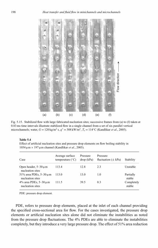
Kandlikar I044527-Ch05.tex 26/10/2005 18: 11 Page 198
198 Heat transfer and fluid flow in minichannels and microchannels
(a) (b) (c) (d) (e) (f)F
low
dire
ctio
nFig. 5.15. Stabilized flow with large fabricated nucleation sites; successive frames from (a) to (f) taken at0.83 ms time intervals illustrate stabilized flow in a single channel from a set of six parallel verticalmicrochannels; water, G = 120 kg/m2 s, q′′ = 308 kW/m2, Ts = 114◦C (Kandlikar et al., 2005).
Table 5.4Effect of artificial nucleation sites and pressure drop elements on flow boiling stability in1054 µm × 197 µm channel (Kandlikar et al., 2005).
Average surface Pressure PressureCase temperature (◦C) drop (kPa) fluctuation (± kPa) Stability
Open header, 5–30 µm 113.4 12.8 2.3 Unstablenucleation sites
51% area PDEs, 5–30 µm 113.0 13.0 1.0 Partiallynucleation sites stable
4% area PDEs, 5–30 µm 111.5 39.5 0.3 Completelynucleation sites stable
PDE: pressure drop element.
PDE, refers to pressure drop elements, placed at the inlet of each channel providingthe specified cross-sectional area for flow. For the cases investigated, the pressure dropelements or artificial nucleation sites alone did not eliminate the instabilities as notedfrom the pressure drop fluctuations. The 4% PDEs are able to eliminate the instabilitiescompletely, but they introduce a very large pressure drop. The effect of 51% area reduction

Kandlikar I044527-Ch05.tex 26/10/2005 18: 11 Page 199
Chapter 5. Flow boiling in microchannels and minichannels 199
in conjunction with the artificial nucleation sites is interesting to note. There was littlepressure drop increase due to area reduction as compared to the fully open channel. Itis therefore possible to arrive at an appropriate area reduction in conjunction with theartificial nucleation sites with marginal increase in the pressure drop.
5.7. Predicting heat transfer in microchannels
Flow boiling heat transfer data was obtained by a number of investigators. Many of theresearchers reported unstable operating conditions during their tests. Therefore, this dataand the matching correlations should be used with some degree of caution.At the same time,it is recommended that experimental data under stable operating conditions be obtained byproviding artificial nucleation sites and pressure drop elements near the inlet inside eachchannel.
A good survey of available experimental data and correlations is provided by Qu andMudawar (2004), and Steinke and Kandlikar (2004). Table 5.3 is adapted from Steinke andKandlikar (2004), and lists the ranges of experimental data available in the literature. Itcan be seen that the fluids investigated include: water, R-21, R-22, R-113, R-123, R-124,R-141b, FC-84, and Vertrel XF. The mass fluxes, liquid Reynolds numbers, and heat fluxesrange from 20 to 6225 kg/m2 s, 14 to 5236, and up to 2 MW/m2, respectively. As the tubediameter decreases, the Reynolds number shifts toward a lower value.
In order to establish the parametric trends, the local flow boiling heat transfer data areneeded. In the papers listed in Table 5.3, only those by Hetsroni et al. (2002), Yen et al.(2002), and Steinke and Kandlikar (2004) deal with tubes around 200 µm and report localheat transfer data. Qu and Mudawar (2003) also report local data for parallel rectangularchannels of 349 µm hydraulic diameter.
The experimental data of Bao et al. (2000) for a 1.95 mm diameter tube indicatesa strong presence of the nucleate boiling term, while Qu and Mudawar’s data exhibits astrong influence of mass flux, indicating the presence of convective boiling. The decreasingtrends in heat transfer coefficient with quality seen in Qu and Mudawar’s data was alsoseen in Steinke and Kandlikar’s (2004) data. A number of issues arise that make it difficultto assess the available experimental data accurately. Some of the factors are:
(i) the presence of instabilities during the experiments,(ii) different ranges of parameters, especially heat flux and mass flux.
The influence of instabilities was discussed in the earlier sections. The ranges of massfluxes employed in small diameter channels typically fall in the laminar range. The corre-lations developed for large diameter tubes are in a large part based on the turbulent flowconditions for Reynolds numbers based on all-liquid flow.
Some of the data available in literature was seen to be correlated by the all-nucleateboiling-type correlations, such as Lazarek and Black (1982), and Tran et al. (1996). How-ever, recent data reported by Qu and Mudawar has very large errors (36.2% and 98.8%).Similar observations can be made with the Steinke and Kandlikar (2004) data. Some ofthe more recent correlations by Yu et al. (2002) and Warrier et al. (2002) employ only theheat flux dependent terms (similar to Lazarek and Black (1982), and Tran et al. (1996))and correlate Qu and Mudawar’s (2003) data well. However, the presence of both nucleate

Kandlikar I044527-Ch05.tex 26/10/2005 18: 11 Page 200
200 Heat transfer and fluid flow in minichannels and microchannels
boiling and convective boiling terms to a varying degree is reported by Kandlikar andBalasubramanian (2004). They recommend using the laminar flow equations for the all-liquid flow heat transfer coefficients in the Kandlikar (1990) correlation and cover a widerange of data sets.
The flow boiling correlation by Kandlikar (1990) utilizes the all-liquid flow, single-phase correlation. Since most of the available data was in the turbulent region, use of theGnielisnki correlation was recommended. However, later, Kandlikar and Steinke (2003),and Kandlikar and Balasubramanian (2004) introduced the laminar flow equation for lam-inar flow conditions based on ReLO. The correlation based on the available data is givenbelow:
For ReLO > 100:
hTP = larger of{
hTP,NBDhTP,CBD
(5.21)
hTP,NBD = 0.6683Co−0.2(1 − x)0.8hLO + 1058.0Bo0.7(1 − x)0.8FFlhLO (5.22)
hTP,CBD = 1.136Co−0.9(1 − x)0.8hLO + 667.2Bo0.7(1 − x)0.8FFlhLO (5.23)
where Co = [(1 − x)/x]0.8(ρV/ρL)0.5and Bo = q′′/GhLV. The single-phase all-liquid flowheat transfer coefficient hLO is given by:
for 104 ≤ ReLO ≤ 5 × 10⁶ hLO = ReLO PrL ( f/2)(kL/D)
1 + 12.7(Pr2/3L − 1)( f/2)0.5
(5.24)
for 3000 ≤ ReLO ≤ 104 hLO = (ReLO − 1000) PrL ( f/2)(kL/D)
1 + 12.7(Pr2/3L − 1)( f/2)0.5
(5.25)
for 100 ≤ ReLO ≤ 1600 hLO = NuLO k
Dh(5.26)
In the transition region between Reynolds numbers of 1600 and 3000, a linear interpolationis suggested for hLO.
For Reynolds number below and equal to 100 (Re ≤ 100) the nucleate boilingmechanism governs, and the following Kandlikar Correlation is proposed,
For ReLO ≤ 100,
hTP = hTP,NBD = 0.6683Co−0.2(1 − x)0.8hLO + 1058.0Bo0.7(1 − x)0.8FFlhLO
(5.27)
The single-phase all-liquid flow heat transfer coefficient hLO in Eq. (5.27) is found fromEq. (5.26).
The fluid surface parameter FFL in Eqs. (5.22), (5.23), and (5.27) for different fluidsurface combinations is given in Table 5.5. These values are for copper or brass surfaces.For stainless steel surfaces, use FFL = 1.0 for all fluids. For silicon surfaces, no data iscurrently available. Use of the values listed in Table 5.5 for copper is suggested.

Kandlikar I044527-Ch05.tex 26/10/2005 18: 11 Page 201
Chapter 5. Flow boiling in microchannels and minichannels 201
Table 5.5Recommended FFl (fluid surface parameter)values in flow boiling correlation by Kandlikar(1990; 1991).
Fluid FFl
Water 1.00R-11 1.30R-12 1.50R-13B1 1.31R-22 2.20R-113 1.30R-114 1.24R-134a 1.63R-152a 1.10R-32/R-132 3.30R-141b 1.80R-124 1.00Kerosene 0.488
0
1000
2000
3000
4000
5000
6000
7000
0.0 0.2 0.4 0.6 0.8 1.0
Quality (x)
hT
P (
W/m
2 K
)
q1 = 5 kW/m2
q2 = 15 kW/m2
q1 – Kandlikar (90)
q2 – Kandlikar (90)
�
�
�
�
Fig. 5.16. Yan and Lin (1998) data points for R-134a compared to the correlation by Kandlikar andBalasubramanian (2004) using the laminar single-phase equation; Dh = 2 mm, G = 50 kg/m2s, q′′ = 5and 15 kW/m2, ReLO = 506.
The above correlation scheme is based on the data available in the literature. It has tobe recognized that all of the data suffer from the instability condition to some extent. It isexpected that the correlation will undergo some changes as new data under stabilized flowconditions become available.
A comparison of the correlation scheme described in Eqs. (5.21)–(5.27) with some ofthe experimental data available in the literature is shown in Figs 5.16–5.18. The decreasing
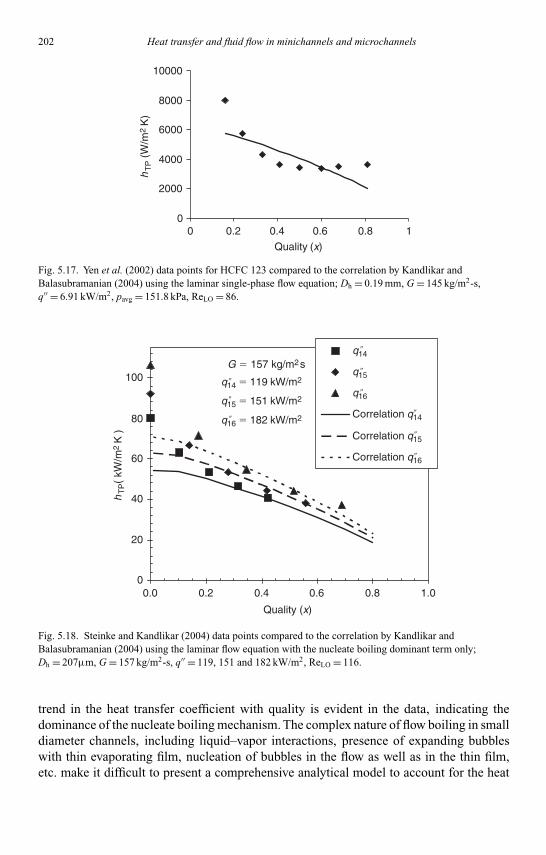
Kandlikar I044527-Ch05.tex 26/10/2005 18: 11 Page 202
202 Heat transfer and fluid flow in minichannels and microchannels
0
2000
4000
6000
8000
10000
0 0.2 0.4 0.6 0.8 1
Quality (x)
hT
P (
W/m
2 K
)
Fig. 5.17. Yen et al. (2002) data points for HCFC 123 compared to the correlation by Kandlikar andBalasubramanian (2004) using the laminar single-phase flow equation; Dh = 0.19 mm, G = 145 kg/m2-s,q′′ = 6.91 kW/m2, pavg = 151.8 kPa, ReLO = 86.
G � 157 kg/m2s
q14 � 119 kW/m2
q15 � 151 kW/m2
q16 � 182 kW/m2
0
20
40
60
80
100
0.0 0.2 0.4 0.6 0.8 1.0
Quality (x)
hT
P(
kW/m
2 K
)
q14
q15
q16
Correlation q14
Correlation q15
Correlation q16
�
�
�
�
�
�
��
�
Fig. 5.18. Steinke and Kandlikar (2004) data points compared to the correlation by Kandlikar andBalasubramanian (2004) using the laminar flow equation with the nucleate boiling dominant term only;Dh = 207µm, G = 157 kg/m2-s, q′′ = 119, 151 and 182 kW/m2, ReLO = 116.
trend in the heat transfer coefficient with quality is evident in the data, indicating thedominance of the nucleate boiling mechanism. The complex nature of flow boiling in smalldiameter channels, including liquid–vapor interactions, presence of expanding bubbleswith thin evaporating film, nucleation of bubbles in the flow as well as in the thin film,etc. make it difficult to present a comprehensive analytical model to account for the heat

Kandlikar I044527-Ch05.tex 26/10/2005 18: 11 Page 203
Chapter 5. Flow boiling in microchannels and minichannels 203
transfer mechanisms during flow boiling. Further efforts with high-speed flow visualizationtechniques are recommended to provide the fundamental information on this topic.
5.8. Pressure drop during flow boiling in microchannels and minichannels
The pressure drop in a microchannel or a minichannel heat exchanger is the sum of thefollowing components:
p = pc +pf ,1-ph +pf ,tp +pa +pg +pe (5.28)
where subscripts c: contraction at the entrance; f,1-ph: single-phase pressure loss dueto friction, including entrance region effects; f,tp: two-phase frictional pressure drop; a:acceleration associated with evaporation; g: gravitational; and e: expansion at the outlet.Equations for calculating each of these terms are presented in the following sections.
5.8.1. Entrance and exit losses
The inlet to the microchannel may be single-phase liquid or a two-phase mixture. It iscommon to have liquid at the inlet when a liquid pump and a condenser are employed in thecooling system. When the refrigeration system forms an integral part of the cooling system,the refrigerant is throttled prior to entry into the microchannels. With the need to incorporatepressure drop elements in each channel, liquid at the inlet in such cases is also possible.
The contraction losses in the single-phase liquid are covered in Chapter 3. The nature ofthe liquid’s entry into the channels is another factor that needs to be taken into consideration.The channel floor may be flush with the manifold, or may be shallower or deeper than themanifold. Lee and Kim (2003) used a micro-PIV system to identify the entrance losseswith sharp and smooth channel entrances.
For the two-phase entry and exit losses, Coleman (2003) recommends the followingscheme proposed by Hewitt (2000).
The following equation is used to calculate the pressure loss due to a sudden contractionof a two-phase mixture using a separated flow model:
pc = G2
2ρL
[(1
Co− 1
)2
+ 1 − 1
σ2c
]ψh (5.29)
where G: mass flux, σc: contraction area ratio (header to channel> 1), Co – contractioncoefficient given by:
Co = 1
0.639(1 − 1/σc)0.5 + 1(5.30)
and ψh: two-phase homogeneous flow multiplier given by:
ψh = [1 + x(ρL/ρV − 1)] (5.31)
with x: local quality.

Kandlikar I044527-Ch05.tex 26/10/2005 18: 11 Page 204
204 Heat transfer and fluid flow in minichannels and microchannels
The exit pressure loss is calculated from the homogeneous model:
pe = G2σe(1 − σe)ψs (5.32)
where σe: area expansion ratio (channel to header< 1), and ψs: the separated flowmultiplier given by:
ψs = 1 +(ρL
ρV− 1
)[0.25x(1 − x) + x2] (5.33)
The frictional pressure drop in the single-phase region prior to nucleation is calculated fromthe equations presented in Chapter 3. In the two-phase region, the following equations maybe used to calculate the frictional, acceleration and gravity components of the pressure drop.
The local friction pressure gradient at any section is calculated with the followingequation:(
dpF
dz
)=(
dpF
dz
)Lφ2
L (5.34)
The two-phase multiplier φ2L is given by the following equation by Chisholm (1983):
φ2L = 1 + C
X+ 1
X 2 (5.35)
The value of the constant C depends on whether the individual phases are in the laminaror turbulent region. Chisholm recommended the following values of C:
Both phases turbulent C = 21 (5.36a)
Laminar liquid, turbulent vapor C = 12 (5.36b)
Turbulent liquid, laminar vapor C = 10 (5.36c)
Both phases laminar C = 5 (5.36d)
The Martinelli parameter X is given by the following equation:
X 2 =(
dpF
dz
)L
/(dpF
dz
)V
(5.37)
Mishima and Hibiki (1996) found that the constant C depends on the tube diameter, andrecommended the following equation for C:
C = 21(1 − e−319Dh ) (5.38)
where Dh is in m. Mishima and Hibiki’s correlation is used extensively and is recommended.English and Kandlikar (2005) found that their adiabatic air–water data in a 1-mm squarechannel was overpredicted by using Eq. (5.38). Upon further investigation, they found that

Kandlikar I044527-Ch05.tex 26/10/2005 18: 11 Page 205
Chapter 5. Flow boiling in microchannels and minichannels 205
0
2
4
6
8
10
12
0.25 0.35 0.45 0.55 0.65 0.75 0.85 0.95
Mass quality (x)
Pre
ssur
e dr
op (
kPa/
m)
Mishima-HibikiExperimental dataEnglish and Kandlikar (2005)
Fig. 5.19. Comparison of experimental data from English and Kandlikar (2005) with their correlation, andMishima and Hibiki’s correlation (1996).
the diameter correction recommended by Mishima and Hibiki (1996) should be appliedto C in Eq. (5.35). Accordingly, the value of C will change depending on the laminar orturbulent flow of individual phases. Thus the following modified equation is recommendedfor frictional pressure drop calculation in microchannels and minichannels:
φ2L = 1 + C(1 − e−319Dh )
X+ 1
X 2 (5.39)
The value of C is obtained from Eqs. (5.36a)–(5.36d).Figure 5.19 shows the agreement of experimental data obtained by English and
Kandlikar (2005) during air–water flow in a 1-mm square channel. The average abso-lute deviation was found to be 3.5%, which was within the experimental uncertainties.Further validation of Eq. (5.39) is recommended.
The acceleration pressure drop is calculated from the following equation assuminghomogeneous flow:
pa = G2vLVxe (5.40)
where vLV: difference between the specific volumes of vapor and liquid phases = vV − vL.The above equation assumes the inlet flow to be liquid only and exit quality to be xe. For atwo-phase inlet flow, the xe should be replaced with the change in quality between the exitand inlet sections.

Kandlikar I044527-Ch05.tex 26/10/2005 18: 11 Page 206
206 Heat transfer and fluid flow in minichannels and microchannels
0.01
0.1
1
10
0.01
0.1
1
10
0.01 0.1 1 10 100 0.01 0.1 1 10 100
Superficial gas velocity (m/s)
Sup
erfic
ial l
iqui
d ve
loci
ty (
m/s
)
Sup
erfic
ial l
iqui
d ve
loci
ty (
m/s
)
D � 2.05 mm
SlugBubbly AnnularChurn
Superficial gas velocity (m/s)
D � 4.08 mm
SlugBubbly Churn Annular
Fig. 5.20. Flow pattern map for minichannels derived from Mishima and Hibiki (1996).
The gravitational pressure drop will be a very small component. It can be calculatedfrom the following equation based on the homogeneous flow model:
pg = g( sin β)L
vLVxeln(
1 + xevLV
vL
)(5.41)
Equation (5.41) also assumes a liquid inlet condition. In case of two-phase inlet flow, thedifference between the exit and inlet quality should be used in place of xe.
5.9. Adiabatic two-phase flow
Adiabatic two-phase flow has been studied extensively in literature, especially with air–water flow. For small diameter channels, the work of Mishima and Hibiki (1996) isparticularly noteworthy. Figure 5.20 shows their flow pattern map.
The effect of surfactants on the adiabatic two-phase flow pressure drop was studiedby English and Kandlikar (2005) in a 1-mm square minichannel with air and water withsuperficial gas and liquid velocities of 3.19–10 m/s and 0.001–0.02 m/s, respectively. Theresulting flow pattern was stratified (annular) in all cases, which is near the bottom rightcorner in Fig. 5.20. The pressure drop was not affected by variation in surface tension from0.034 to 0.073 N/m. The reason for this is believed to be the absence of a three-phase line(such as would exist with discrete droplets sliding on the wall). The Mishima and Hibiki(1996) correlation for pressure drop was modified as shown in Fig. 5.19 using Eqs. (5.39)and (5.36).
5.10. Practical cooling systems with microchannels
Use of microchannels in a high heat flux cooling application using flow boiling systemswas reviewed by Pokharna et al. (2004) for notebook computers and for server applicationsby Kandlikar (2005). The major issues that need to be addressed before implementationof flow boiling becomes practical are listed as follows (Kandlikar, 2005).
Kandlikar I044527-Ch05.tex 26/10/2005 18: 11 Page 207
Chapter 5. Flow boiling in microchannels and minichannels 207
High heat flux cooling systems with flow boiling have lagged behind the single-phaseliquid cooled systems because of some of the operational challenges that still remain to beresolved. These are listed below:
(i) Need for low-pressure water or a suitable refrigerant to match the saturationtemperature requirement for electronics cooling.
(ii) Unstable operation due to rapid bubble expansion and occasional flow reversal.(iii) Unavailability of CHF data and a lack of fundamental understanding of the flow
boiling phenomenon in microchannel passages.
The use of water is very attractive from a heat transfer performance perspective, butthe positive pressure requirement may lead to a vacuum system, which is generally notdesirable due to possible air leakage, which raises the saturation temperature in the system.Development of a suitable refrigerant suitable for this application is recommended.
The desirable characteristics of an ideal refrigerant in a flow boiling system may belisted as (Kandlikar, 2005):
(a) saturation pressure slightly above the atmospheric pressure at operating temperatures;(b) high latent heat of vaporization;(c) good heat transfer and pressure drop related properties (high liquid thermal conduc-
tivity, low liquid viscosity, low hysteresis for ONB);(d) high dielectric constant if applied directly into the chip;(e) compatible with silicon (for direct chip cooling) and copper (for heat sink applications),
and other system components;(f) low leakage rates through pump seals;(g) chemical stability under system operating conditions;(h) low cost;(i) safe for human and material exposure under accidental leakages.
The fundamental understanding of the flow boiling phenomenon is slowly emerging,and efforts to stabilize the flow using nucleating cavities and pressure drop elements isexpected to help in making flow boiling systems as a viable candidate for high heat fluxcooling application.
Another application for flow boiling in narrow channels is in compact evaporators.The evaporators used in automotive application currently do not employ some of thesmall channel configurations used in condenser application due to stability problems.Stabilized flow boiling, as described in Section 5.6, will enable practical implementationof microchannels and minichannels in a variety of compact evaporator applications.
5.11. Solved examples
Example 5.1
Water is used as the cooling liquid in a microchannel heat sink. The dimensions of onechannel are a = 1054 µm × b = 50 µm, where a is the unheated length in the three-sidedheating case. The inlet temperature of the water is 70◦C, and the Reynolds number in thechannel is 600.
Kandlikar I044527-Ch05.tex 26/10/2005 18: 11 Page 208
208 Heat transfer and fluid flow in minichannels and microchannels
(1) Calculate the insipient boiling location and cavity radius and plot the wall superheatand liquid subcooling at the ONB versus the cavity radius rc. Also plot the predictedheat transfer coefficient as a function of quality for the following values of heat flux:
(i) q′′ = 50 kW/m2, (ii) q′′ = 340 kW/m2, (iii) q′′ = 1 MW/m2.
(2) Calculate the pressure drop in the heat exchanger core for a heat flux of 1 MW/m2 anda channel length of 20 mm.
AssumptionsFully developed laminar flow Nusselt number; three-sided heating; properties of water areat saturation temperature at 1 atm; Receding contact angle is 40◦.
SolutionProperties of water at 100◦C: hLV = 2.26 × 10⁶ J/kg, iL = 4.19 × 10⁵ J/kg, ρV =0.596 kg/m3, vL = 0.001044 m3/kg, vg = 1.679 m3/kg, cp,L = 4217 J/kg-K, µV = 1.20 ×10⁻⁵ N-s/m2, µL = 2.79 × 10⁻⁴ N-s/m2, kL = 0.68 W/m-K, σ= 0.0589 N/m, Pr = 1.76(Incropera and DeWitt, 2002). Properties of water at 70◦C: iL = 2.93 × 10⁵ J/kg.
Part 1(i) Heat flux is 50 kW/m2
The fully developed Nusselt number is found using Table 3.3 with aspect ratioαc = a/b = 1054 µm/50 µm = 21.08. Since the aspect ratio is greater than 10, the Nusseltnumber for three-sided heating is 5.385. The hydraulic diameter and heated perimeter are:
Dh = 4Ac
Pw= 2ab
(a + b)= 2 × 1054 × 10−6 × 50 × 10−6
(1054 + 50) × 10−6 = 9.547 × 10⁻⁵ m
= 95.47 µm
P = a + 2b = (2 × 50 + 1054) × 10−6 = 1.154 × 10⁻³ m = 1154 µm
The heat transfer coefficient is h = kLNu/Dh = (0.68 W/m-K)(5.385)/(9.55 × 10−5 m) =38,355 W/m2-K.
Under the fully developed assumption, a value for the temperature difference betweenthe wall temperature and the bulk liquid temperature can be found using the equa-tion q′′ = h(T ) = h(TWall − TBulk) = h(TWall − TSat + TSat − TBulk) = h(TSat +TSub).Therefore, the sum of TSat and TSub can be found for a given heat flux asq′′/h = (TSat +TSub) = (50,000 W/m2)/(38,355 W/m2-K) = 1.30◦C.
The wall superheat at the critical cavity radius is found by setting the expression underthe radical in Eq. (5.16) equal to zero.
√1 − [8.8σTSat(TSat +TSub)]/(ρVhLVδtT 2
Sat) = 0
Noting that δt = kL/h, the equation q′′ = h(TSat +TSub) can be written as q′′ =kLδt
(TSat +TSub).

Kandlikar I044527-Ch05.tex 26/10/2005 18: 11 Page 209
Chapter 5. Flow boiling in microchannels and minichannels 209
Solving this equation for δt :
δt = kL(TSat +TSub)/q′′ = (0.68 × 1.3)/50,000 = 1.77 × 10⁻⁵m = 17.7 µm
and substituting it into the expression under the radical in Eq. (5.16), the value for TSatat the critical rc can be obtained as:
TSat =√
8.8σTSatq′′ρVhLVkL
=√
8.8 × 0.0589 × 373.15 × 50,000
0.596 × 2.26 × 106 × 0.68= 3.25◦C
The cavity radius can be found by using Eq. (5.17):
rc,crit =(δt sin θr
2.2
)(TSat
TSat +TSub
)=(
1.77 × 10⁻⁵ × sin 40◦
2.2
)3.25
1.3
= 12.9 × 10⁻⁶ m = 12.9 µm
Using Eq. (5.1) and the definitions of wall superheat and liquid subcooling given byEqs. (5.8) and (5.9), the location where ONB occurs is found:
z = (TB,z − TB,i)mcp
q′′P= (375.1 − 343.15) × 92.4 × 10−6 × 4217
50,000 × 1.15 × 10−3
= 0.216 m = 21.6 cm
Realistically, this length is too large for a microchannel heat exchanger and the actuallength is expected to be much shorter. Also, the heat flux is very low for a microchannelheat exchanger. Therefore, it will be operating under single-phase liquid flow conditionsthroughout. Plotting Eq. (5.16) as a function of TSat illustrates the nucleation criteriafor the given heat flux. The wall superheat at ONB is plotted as a function of the nucle-ation cavity radius (TONB versus rc) by using Eq. (5.20). The liquid subcooling is alsopresented on this plot. Note that the negative values of TSub indicate that the bulk issuperheated at the point of nucleation. This will lead to significant flow instabilities asdiscussed in the Section 5.4.
Nucleation criteria
1
10
100
0 10 20 30�TSat (°C)
Cav
ity r
adiu
s (µ
m)
�TONB versus rc
�20�15�10
�505
1015
20
0.1 1 10 100rc (µm)
�T
ON
B (
°C)
rc,min
rc,max
�TSat,ONB
�TSub,ONB

Kandlikar I044527-Ch05.tex 26/10/2005 18: 11 Page 210
210 Heat transfer and fluid flow in minichannels and microchannels
The Boiling number is calculated from Table 5.1:
Bo = q′′
GhLV= q′′Dh
hLV ReµL= 50,000 × 9.547 × 10−5
2.26 × 106 × 600 × 2.79 × 10−4 = 1.262 × 10⁻⁵
For a flow of higher Reynolds number, the value of hLO would not be the same as thesingle-phase value of h, as can be seen with Eqs. (5.24)–(5.26). As the Reynolds number is600, the heat transfer coefficient hLO is equal to the single-phase value of h by Eq. (5.26),hLO = h = 38,355 W/m2 K.
The Convection number is a function of quality:
Co = [(1 − x)/x]0.8[ρV/ρL]0.5 = [(1 − x/x)]0.8(0.596/957.9)
= [(1 − x)/x]0.8 × 6.22 × 10−4
From Eq. (5.21), the flow boiling hTP is the larger of Eqs. (5.22) and (5.23), which canbe plotted as functions of x as seen below using an FFl of 1:
hTP = larger of{
hTP,NBDhTP,CBD
hTP,NBD = hLO[0.6683Co−0.2(1 − x)0.8 + 1058.0Bo0.7(1 − x)0.8FFl]
= 38,355{0.6683([(1 − x)/x]0.8 × 6.22 × 10−4)−0.2(1 − x)0.8
+ 1058.0(1.262 × 10⁻⁵)0.7(1 − x)0.8 × 1}hTP,CBD = hLO[1.136Co−0.9(1 − x)0.8 + 667.2Bo0.7(1 − x)0.8FFl]
= 38,355{1.136([(1 − x)/x]0.8 × 6.22 × 10−4)−0.9(1 − x)0.8
+ 667.2(1.262 × 10⁻⁴)0.7(1 − x)0.8 × 1}
Predicted heat transfer coefficientversus quality
0.0E�00
2.0E�05
4.0E�05
6.0E�05
8.0E�05
1.0E�06
1.2E�06
0 0.2 0.4 0.6 0.8 1Quality (x )
h TP (
W/m
2 K
)
NBD
CBD
Since hTP,NBD yields higher values than hTP,CBD, it represents the flow boiling thermalconditions and should be used for the present case. Note that hTP increases with qualityfor this case.

Kandlikar I044527-Ch05.tex 26/10/2005 18: 11 Page 211
Chapter 5. Flow boiling in microchannels and minichannels 211
(ii) Heat flux is 340 kW/m2
a = 1054 µm; b = 50 µm; Ti = 70◦C; Re = 600; αc = 21.08; h = 38,355 W/m2 K(TSat +TSub) = 8.86◦C; TSat = 8.48◦C; rc,crit = 5.0 µm; z = 2.9 cm
Nucleation criteria
1
10
100
Predicted heat transfer coefficient versus quality
rc,min
rc,max
�TSat,ONB
�TSub,ONB�20
�15
�10
�5
0
5
10
15
20
�T
ON
B (
°C)
0 10 20 30�TSat (°C)
�TONB versus rc
0.1 1 10 100
rc (µm)
Cav
ity r
adiu
s (µ
m)
0 0.2 0.4 0.6 0.8 1Quality (x)
0.0E�00
2.0E�05
4.0E�05
6.0E�05
8.0E�05
1.0E�06
1.2E�06
h TP (
W/m
2 K
)
NBD
CBD
In plotting the heat transfer coefficient versus quality, it is seen that the nucleate boilingdominant prediction is actually higher than the convective dominant prediction for verylow qualities (<0.1) and should be used in those cases. There is an increase in the nucleateboiling behavior in comparison to the lower heat flux case.
(iii) Heat flux is 1 MW/m2
a = 1054 µm; b = 50 µm; Ti = 70◦C; Re = 600; αc = 21.08; h = 38,355 W/m2 K(TSat +TSub) = 26.1◦C; TSat = 14.5◦C; rc,crit = 2.9 µm; z = 0.6 cm
The nucleate boiling dominant prediction is higher than the convective boiling dominantfor qualities lower than 0.4 and should be used for those cases. Note that a high wallsuperheat is needed to initiate nucleation (14.5◦C). Also, the cavity sizes for nucleationbecome smaller as the heat flux increases. Thus a variety of different cavity sizes areneeded on a surface to operate it at different heat flux conditions. Another point to noteis that the saturation temperature of water at 1 atm is quite high for electronics coolingapplications. Two options can be pursued: one is to use low-pressure steam, and the otheris to use refrigerants. The next example illustrates the use of refrigerants.

Kandlikar I044527-Ch05.tex 26/10/2005 18: 11 Page 212
212 Heat transfer and fluid flow in minichannels and microchannels
Predicted heat transfer coefficientversus quality
rc,min
rc,max
�TSat,ONB
�TSub,ONB
�20�15�10
�5
05
1015202530
�T
ON
B (
°C)
0 10 20 30 40�TSat (°C)
Nucleation criteria �TONB versus rc
0.1 1 10 100
rc (µm)
1
10
100
Cav
ity r
adiu
s (µ
m)
0.0E�00
2.0E�05
4.0E�05
6.0E�05
8.0E�05
1.0E�06
1.2E�06
1.4E�06
0 0.2 0.4 0.6 0.8 1Quality (x)
h TP (
W/m
2 K
)
NBD
CBD
Part 2From Part 1, (iii), it is found that the onset of nucleate boiling occurs at 0.6 cm from theentrance end. Therefore, the flow is single-phase up to 0.6 cm at which point it becomestwo-phase flow. However, the bulk is subcooled at this location and so Eq. (5.1) is used todetermine the location where the saturation temperature is reached:
z = (TB,z − TB,i)mcp
q′′P= (100 − 70) × 92.4 × 10−6 × 4217
1 × 106 × 1.15 × 10−3 = 0.0101 m = 1.01 cm
Using this approach simplifies the problem, but keep in mind that since ONB actuallyoccurs before this location in the channel, the actual pressure drop in the core of thechannel will be slightly higher due to the longer two-phase flow length.
The exit quality can be solved for by using the following equation to get xe = 0.055,where AT is the heated perimeter multiplied by the channel length:
q′′AT = m[(iL,@TSat + xehLV,@TSat ) − iL,@TB,in ]

Kandlikar I044527-Ch05.tex 26/10/2005 18: 11 Page 213
Chapter 5. Flow boiling in microchannels and minichannels 213
xe =(
q′′AT
m+ iL,@TB,in − iL,@TSat
)/hLV,@TSat
=(
10,00,000 × 1.15 × 10−3 × 0.02
9.24 × 10⁻⁵ + 2.93 × 10⁵ − 4.19 × 10⁵)/
2.26 × 106
= 0.055
The total mass flux can be calculated from the Reynolds number and channel geometry:
G = ReµL/Dh = (600 × 2.79 × 10−4)/(9.547 × 10−5) = 1753 kg/m2s
The superficial Reynolds numbers of the liquid and vapor phases in the two-phase flowregion are found by using the following equations. The average quality over the channellength is taken as half the exit quality.
ReV = G xe2 Dh
µV= 1753 × 0.055
2 × 9.547 × 10−5
1.2 × 10−5 = 384
ReL = G(1 − xe
2
)Dh
µL= 1753
(1 − 0.055
2
)9.547 × 10⁻⁵
2.79 × 10−4 = 583
The single-phase friction factors fL and fV are obtained by using Eq. (3.10) with theReynolds numbers calculated above.
Po = f Re = 24(1 − 1.3553αc + 1.9467α2c − 1.7012α3
c + 0.9564α4c − 0.2537α5
c)
= 24(1 − 1.3553 × 21.08 + 1.9467 × 21.082 − 1.7012 × 21.083
+ 0.9564 × 21.084 − 0.2537 × 21.085)
= 22.56
The friction pressure gradients given in Eq. (5.37) are defined as:
−(
dpF
dz
)L
= 2fLG2(1 − xe
2
)2DhρL
= 2( 22.56
583
)17532
(1 − 0.055
2
)29.547 × 10−5 × 957.9
= 2,458,697 Pa/m = 2.46 MPa/m
−(
dpF
dz
)V
= 2fVG2( xe
2
)2DhρV
= 2( 22.56
384
)17532
( 0.0552
)29.547 × 10−5 × 0.5956
= 4,800,308 Pa/m = 4.80 MPa/m
X 2 =(
dpF
dz
)L
/(dpF
dz
)V
= 2.46
4.80= 0.5125

Kandlikar I044527-Ch05.tex 26/10/2005 18: 11 Page 214
214 Heat transfer and fluid flow in minichannels and microchannels
The two-phase multiplier is calculated with Eq. (5.39):
φ2L = 1 + C
(1 − e−319Dh
)X
+ 1
X 2 = 1 +5(
1 − e−319×9.547×10−5)
√0.5125
+ 1
0.5125= 3.16
and the two-phase pressure drop per unit length is calculated with Eq. (5.34):(dpF
dz
)TP
=(
dpF
dz
)Lφ2
L = 24,58,697 × 3.16 = 7,769,482 Pa/m = 7.77 MPa/m
The frictional two-phase pressure drop is found by multiplying the frictional pressuregradient by the two-phase flow length (0.02 m – 0.0101 m = 0.0099 m) to get 76.7 kPa.
The total pressure drop in the core is found by adding the pressure drop in the single-phase flow section length (0.0101 m) and the two-phase pressure drop:
p = pf ,1-ph +pf ,tp = 26,800 + 76,700 = 103,500 Pa = 103.5 kPa (15.0 psi)
Example 5.2
Microchannels are directly etched into the silicon chips to dissipate a heat flux of13,000 W/m2 from a computer chip. The geometry may be assumed similar to Fig. 3.19.Each of the parallel microchannels has a width a = 200 µm, height b = 200 µm, andlength L = 10 mm. Refrigerant-123 flows through the horizontal microchannels at an inlettemperature of TB,i = 293.15 K. The heated perimeter P = b + a + b = 600 × 10−6 m, andthe cross-sectional area Ac = a × b = 40 × 10−9 m. Assume θr from Fig. 5.1 is 20◦, andRe = 100.
SolutionProperties of R-123 at TSat = 300.9 K and 1 atm: µL = 404.2 × 10⁻⁶ N-s/m2,µV = 10.8 × 10⁻⁶ N-s/m2, ρL = 1456.6 kg/m3, ρV = 6.5 kg/m3, cp,L = 1023 J/kg K, kL =75.6 × 10⁻³ W/m K, kV = 9.35 × 10⁻³ W/m K, σL = 14.8 × 10⁻³ N/m, hLV = 170.19 ×10³ J/kg, iL = 228 × 103 J/kg, iV = 398 × 103 J/kg.
(i) Calculate the incipient boiling location and cavity radius (Answers: z = 0.584 ×10⁻³ m, and rc,crit = 2.23 × 10⁻⁶ m)From Eq. (5.18):
TSat,ONB = √8.8σTSatq′′/(ρVhLVkL)
=√
8.8(14.8 × 10⁻³)(300.9)(13,000)/(6.5)(170.19 × 103)(75.6 × 10⁻³)
= 2.47 K
Calculate the hydraulic diameter:
Dh = 4Ac
Pw= a = b = 200 × 10−6 m

Kandlikar I044527-Ch05.tex 26/10/2005 18: 11 Page 215
Chapter 5. Flow boiling in microchannels and minichannels 215
From Table 3.3, Nufd,3 = 3.556, and note that:
h = NukL
Dh= (3.556)(0.0756)
(200 × 10−6)= 1344 W/m2 K
From Eq. (5.19):
TSub,ONB = q′′
h−TSat,ONB = 13,000
1344− 2.47 = 7.2 K
From Eq. (5.8), TB at the onset of nucleate boiling is:
TB,ONB = TSat −TSub,ONB = 300.9 − 7.2 = 293.7 K
Calculate the flow velocity using the Reynolds number:
V = ReµL
ρDh= (100)(404.2 × 10⁻⁶)
(1456.6)(200 × 10−6)= 0.139 m/s
Calculate the mass flow rate:
m = ρVAc = (1456.6)(0.139)(40 × 10−9) = 8.09 × 10⁻⁶ kg/s
Calculate the mass flux:
G = m
Ac= 8.09 × 10⁻⁶
40 × 10−9 = 202 kg/m2 s
The incipient boiling location can be calculated by rearranging Eq. (5.1):
z = (TB,ONB − TB,i)(
mcp,L
q′′P
)
= (293.7 − 293.15)(
(8.09 × 10⁻⁶)(1023)
(13,000)(600 × 10−6)
)
= 0.584 × 10⁻³ m
To find the cavity radius, substitute Eqs. (5.3) and (5.19) into Eq. (5.17) we get
rc,crit = kL sin θrTSat,ONB
2.2q′′ = (75.6 × 10⁻³)( sin 20◦)(2.47)
2.2(13,000)= 2.23 × 10⁻⁶ m
(ii) Plot the wall superheat and liquid subcooling versus nucleating cavity radius forq′′ = 5, 13, and 30 kW/m2.Equations (5.19) and (5.20) are used to plot the following figures.
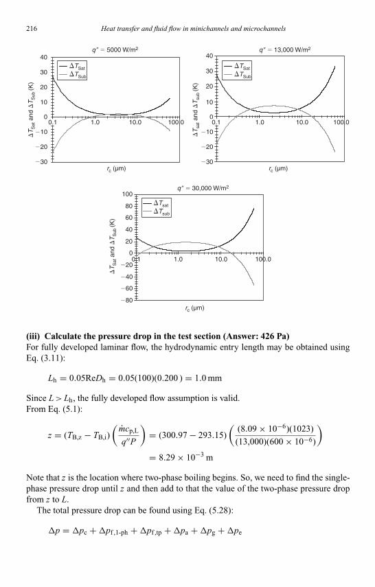
Kandlikar I044527-Ch05.tex 26/10/2005 18: 11 Page 216
216 Heat transfer and fluid flow in minichannels and microchannels
q � � 5000 W/m2 q � � 13,000 W/m2
q � � 30,000 W/m2
�30
�20
�10
0 0
10
20
30
40
0.1 1.0 1.010.0 10.0100.0
100.010.01.00.1
rc (µm) rc (µm)
rc (µm)
�T
Sat
and
�T
Sub
(K)
�T
sat a
nd �
Tsu
b (K
)
�T
Sat
and
�T
Sub
(K)
�30
�20
�10
10
20
30
40
�TSat�TSub
�TSat�TSub
�Tsat�Tsub
.
�80
�60
�40
�20
0
20
40
60
80
100
100.00.1
(iii) Calculate the pressure drop in the test section (Answer: 426 Pa)For fully developed laminar flow, the hydrodynamic entry length may be obtained usingEq. (3.11):
Lh = 0.05ReDh = 0.05(100)(0.200 ) = 1.0 mm
Since L>Lh, the fully developed flow assumption is valid.From Eq. (5.1):
z = (TB,z − TB,i)(
mcp,L
q′′P
)= (300.97 − 293.15)
((8.09 × 10⁻⁶)(1023)
(13,000)(600 × 10−6)
)
= 8.29 × 10⁻³ m
Note that z is the location where two-phase boiling begins. So, we need to find the single-phase pressure drop until z and then add to that the value of the two-phase pressure dropfrom z to L.
The total pressure drop can be found using Eq. (5.28):
p = pc +pf ,1-ph +pf ,tp +pa +pg +pe

Kandlikar I044527-Ch05.tex 26/10/2005 18: 11 Page 217
Chapter 5. Flow boiling in microchannels and minichannels 217
To find the single-phase pressure drop, the f Re term can be obtained using Eq. (3.10) andusing an aspect ratio of one:
αc = a/b = 200/200 = 1
f Re = 24(1 − 1.3553αc + 1.9467α2c − 1.7012α3
c + 0.9564α4c − 0.2537α5
c)
= 24(1 − 1.3553 × 1 + 1.9467 × 12 − 1.7012 × 13 + 0.9564 × 14
− 0.2537 × 15) = 14.23
The single-phase core frictional pressure drop can be calculated using Eq. (3.14):
pf ,1-ph = 2( f Re)µLUmz
D2h
+ K(∞) · ρLU 2m
2where K(∞) is given by Eq. (3.18)
K(∞) = (0.6796 + 1.2197αc + 3.3089α2c − 9.5921α3
c
+ 8.9089α4c − 2.9959α5
c)
= 1.53
pf ,1-ph = 2(14.23)(0.404 × 10⁻³ )(0.139 )(0.00829 )
(200 × 10−6 )2
+ (1.53)(1456.6 )(0.139 )2
2= 353 Pa
Note thatpc, pg andpe can be neglected because we are calculating the core pressuredrop in horizontal microchannels.
The following Eqs. (9.1-12, 14, 35, 36, 37, 39 and 40) are from Chapter 9 of Handbookof Phase Change (Kandlikar et al., 1999). Assuming that the liquid pressure is 1 atm, theniIN = 228 × 103 J/kg. The heated area in the two-phase region is:
Ah,tp = (b + a + b)(L − z) = (200 × 10−6 + 200 × 10−6 + 200 × 10−6)
× (10 × 10−3 − 8.29 × 10⁻³)
= 1.026 × 10⁻⁶ m2
From Eq. (9.1-12):
iTP = iIN + q′′Ah,tp
GAc= 228 × 103 + (13,000)(1.026 × 10⁻⁶)
(8.09 × 10⁻⁶)= 229.6 × 10³ J/kg
From Eq. (9.1-14):
xe = iTP − iLhLV
= (229.6 × 10³ − 228 × 103)
(170.19 × 10³)= 0.0094

Kandlikar I044527-Ch05.tex 26/10/2005 18: 11 Page 218
218 Heat transfer and fluid flow in minichannels and microchannels
Use the average thermodynamic quality between 0 and xe, xavg = 0.0047. FromEq. (9.1-39):
ReV = GxDh
µV= (202)(0.0047)(200 × 10−6)
(10.8 × 10⁻⁶)= 17.58
From earlier the vapor friction factor is:
fV = 14.23
ReV= 14.23
17.58= 0.809
From Eq. (9.1-35):
−(
dpF
dz
)V
= 2fVG2x2
DhρV= 2(0.809)(202)2(0.0047)2
(200 × 10−6)(6.5)= 1122 Pa/m
From Eq. (9.1-40):
ReL = G(1 − x)Dh
µL= (202)(1 − 0.0047)(200 × 10−6)
(0.4042 × 10⁻³)= 99.48
fL = 14.23
ReL= 14.23
99.48= 0.143
From Eq. (9.1-36):
−(
dpF
dz
)L
= 2fLG2(1 − x)2
DhρL= 2(0.143)(202)2(1 − 0.0047)2
(200 × 10−6)(1456.6)= 39,683 Pa/m
From Eq. (5.37):
X 2 =(
dpF
dz
)L
/(dpF
dz
)V
= 39,683
1122= 35.37
Assuming both phases are laminar, from Eq. (5.36d), C = 5.Using Eq. (5.39):
φ2L = 1 + C(1 − e−319Dh )
X+ 1
X 2 = 1 + 5(1 − e−319(200×10−6))√35.37
+ 1
35.37= 1.08
From Eq. (5.34) pf ,tp =(
dpFdz
)=(
dpFdz
)Lφ2
L = (39,683)(1.08) = 42,858 Pa/m
The acceleration pressure drop is calculated from Eq. (5.40):
pa = G2vLVxe = (202)2(0.00069)(0.0094) = 0.26 Pa

Kandlikar I044527-Ch05.tex 26/10/2005 18: 11 Page 219
Chapter 5. Flow boiling in microchannels and minichannels 219
The value of the acceleration pressure drop is negligible, and hence the total pressuredrop is
p = pf ,1-ph +pf ,tp = (353) + (42,858)(0.01 − 0.00829) = 426 Pa
(iv) Plot the predicted heat transfer coefficient as a function of qualityFrom Table 5.1, the Boiling number is:
Bo = q′′
GhLV= (13,000)
(202)(170.19 × 10³)= 0.378 × 10⁻³
From Table 5.1, the convection number is:
Co = [(1 − x)/x]0.8[ρV/ρL]0.5 = [(1 − x)/x]0.8(6.5/1456.6)0.5
= 0.0668[(1 − x)/x]0.8
For ReLO ≤ 100, from Eqs. (5.26) and (5.27):
hLO = NukL
Dh= (3.556)(0.0756)
(200 × 10−6)= 1344 W/m2 K
From Table 3 in page 391 of Handbook of Phase Change (Kandlikar et al., 1999), assumeFFl = 1.3.
For ReLO ≤ 100, hTP = hTP,NBD and we can plot the predicted heat transfer coefficientas a function of quality using Eq. (5.27). This is very similar to the method followedin the previous example, but only the nucleate boiling dominant prediction is used fromEq. (5.27):
hTP = hTP,NBD = hLO{0.6683Co−0.2(1 − x)0.8 + 1058.0Bo0.7(1 − x)0.8FFl}= 1344{0.6683(0.0668[(1 − x)/x]0.8)−0.2(1 − x)0.8
+ 1058.0(0.378 × 10⁻³)0.7(1 − x)0.8FFl}
02000
400060008000
10,00012,000
14,00016,000
0 0.2 0.4 0.6 0.8 1Quality (x)
hT
P (
W/m
2 K
)
hTP,NBD
hTP, NBD

Kandlikar I044527-Ch05.tex 26/10/2005 18: 11 Page 220
220 Heat transfer and fluid flow in minichannels and microchannels
The total frictional pressure drop has to consider the minor losses because the actualp is higher than the core frictional pressure drop. Due to the laminar conditions and thedominance of nucleate boiling effects, note the decreasing trend in hTP as a function ofquality.
5.12. Practice problems
1. A microchannel with dimensions of 120 µm × 400 µm and 3 mm length operates at aninlet pressure of 60 kPa. The inlet liquid is at saturation temperature. A heat flux of600 kW/m2 is applied to the three sides of the channel walls:
(i) Calculate the mass flux to provide an exit quality of 0.1 from this channel.Assuming that cavities of all sizes are available, calculate the distance at whichONB occurs. What is the nucleating cavity diameter at this location?
(ii) Calculate the pressure drop in the channel.(iii) Plot the variation of heat transfer coefficient with channel length assuming an
evaporator pressure to be mean of the inlet and exit pressures.
2. R-123 is used to cool a microchannel chip dissipating 400 W from a chip 12 mm ×12 mm surface area. Assuming an allowable depth of 300 µm, design a cooling systemto keep the channel wall temperature below 70◦C. Calculate the associated pressuredrop in the channel.
3. A copper heat sink has a 60 mm × 120 mm base. It is desired to dissipate 10 kW ofheat while keeping the plate temperature below 130◦C with a flow boiling system usingwater. Design a suitable cooling channel configuration and water flow rate to accomplishthe design.
4. Flow boiling instability in microchannels arises due to rapid bubble growth, especiallynear the inlet of the channels. Identify the relevant parameters that affect the resultinginstability and develop an analytical model to predict the instability condition.
References
Balasubramanian, P. and Kandlikar, S. G., An experimental study of flow patterns, pressure drop andflow instabilities in parallel rectangular minichannels, Heat Transfer Eng., 26(3), 20–27, 2005.
Bao, Z. Y., Fletcher, D. F., and Haynes, B. S., Flow boiling heat transfer of freon R11 and HCFC123in narrow passages, Int. J. Heat Mass Transfer, 43, 3347–3358, 2000.
Bergles, A. E., Forced convection surface boiling heat transfer and burnout in tubes of small diameter,Doctoral Dissertation, Massachusetts Institute of Technology, Cambridge, Massachusetts, 1962.
Bergles, A. E., Subcooled burnout in tubes of small diameter, ASME Paper No. 63-WA-182, 1963.Bergles, A. E. and Kandlikar, S. G., On the nature of critical heat flux in microchannels, J. Heat
Transfer, 127(1), 101–107, 2005.Bergles, A. E. and Rohsenow, W. M., Forced convection surface boiling heat transfer and
burnout in tubes of small diameter, M.I.T. Engineering Projects Laboratory Report No. DSR8767-21, 1962.
Bergles, A. E. and Rohsenow, W. M., The determination forced-convection surface boiling heattransfer, J. Heat Transfer, 86, 365–272, 1964.

Kandlikar I044527-Ch05.tex 26/10/2005 18: 11 Page 221
Chapter 5. Flow boiling in microchannels and minichannels 221
Bonjour, J. and Lallemand, M., Flow patterns during boiling in a narrow space between two verticalsurfaces, Int. J. Multiphase Flow, 24, 947–960, 1998.
Bowers, M. B. and Mudawar, I., High flux boiling in low flow rate, low pressure drop mini-channeland micro-channel heat sinks, Int. J. Heat and Mass Transfer, 37(2), 321–334, 1994.
Brutin, D. and Tadrist, F., Experimental study of unsteady convective boiling in heated minichannels,Int. J. Heat Mass Transfer, 46, 2957–2965, 2003.
Brutin, D., Topin, F., and Tadrist, L., Experimental study on two-phase flow and heat transferin capillaries, in Proceedings of the Twelfth International Heat Transfer Conference, France,pp. 789–784, 2002.
Chisholm, D., Two-Phase Flow in Pipelines and Heat Exchangers, New York: Godwin, 1983.Coleman, J. W., An experimentally validated model for two-phase sudden contraction pressure
drop in microchannel tube headers, in Proceedings of the First International Conference onMicrochannels and Minichannels, ASME Paper No. ICMM2003-1026, April 24–25, Rochester,New York, USA, pp. 241–248, 2003.
Cornwell, K. and Kew, P. A., Boiling in small parallel channels, in Proceedings of CEC Conferenceon Energy Efficiency in Process Technology, Athens, October 1992, Paper 22, Elsevier AppliedSciences, pp. 624–638, 1992.
Cuta, J. M., McDonald, C. E., and Shekarriz, A., Forced convection heat transfer in parallel channelarray microchannel heat exchanger, ASME PID-Vol. 2/HTD-Vol. 338, in Advances in EnergyEfficiency, Heat and Mass Transfer Enhancement, ASME, New York, pp. 17–22, 1996.
Davis, E. J. and Anderson, G. H., The incipience of nucleate boiling in forced convection flow,AIChE J., 12(4), 774–780, 1966.
Downing, R. S., Meinecke, J., and Kojasoy, G., The effects of curvature on pressure drop for singleand two-phase flow in miniature channels, in Proceedings of NHTC2000: 34th National HeatTransfer Conference, Paper No. NHTC2000-12100, August 20–22, Pittsburgh, PA, 2000.
English, N. J. and Kandlikar, S. G., An experimental investigation into the effect of surfactants onair-water two-phase flow in minichannels, in proceedings of the Third International Conferenceon Microchannels and Minichannels, ASME Paper No. ICMM2005-75110, June 13–15, Toronto,Canada, p. 8, 2005.
Faulkner, D. J. and Shekarriz, R., Forced convective boiling in microchannels for kW/cm2 electronicscooling, in Proceedings of ASME Summer Heat Transfer Conference, Paper No. HT2003-47160,July 21–23, Las Vegas, USA: ASME Publications, 2003.
Hetsroni, G., Segal, Z., and Mosyak, A., Nonuniform temperature distribution in electronic devicescooled by flow in parallel microchannels, in Packaging of Electronic and Photonic Devices, IEEETransactions on Components and Packaging Technologies, 24(1), pp. 16–23, 2001.
Hetsroni, G., Mosyak, A., Segal, Z., and Ziskind, G., A uniform temperature heat sink for coolingof electronic devices, Int. J. Heat Mass Transfer, 45, 3275–3286, 2002.
Hetsroni, G., Klein, D., Mosyak, A., Segal, Z., and Pogrebnyak, E., Convective boiling in par-allel microchannels, in Proceeding of the First International Conference on Microchannels andMinichannels, ASME Paper No. ICMM2003-1006, April 24–25, Rochester, NewYork, pp. 59–68,2003.
Hewitt, G. F., Fluid mechanics aspects of two-phase flow, Chapter 9, in Handbook of Boiling and Con-densation, S. G., Kandlikar, M., Shoji, V. K., Dhir, NewYork, NY, USA: Taylor and Francis, 2000.
Hsu, Y. Y., On the size range of active nucleation cavities on a heating surface, J. Heat Transfer, 84,207–216, 1962.
Hsu, Y. Y. and Graham, R., An analytical and experimental study of the thermal boundary layer andebullition cycle in nucleate boiling, NASA TN-D-594, 1961.
Incropera, F. P. and DeWitt, D. P., Fundamentals of Heat and Mass Transfer, 5th Edn., New York:John Wiley and Sons, 2002.

Kandlikar I044527-Ch05.tex 26/10/2005 18: 11 Page 222
222 Heat transfer and fluid flow in minichannels and microchannels
Jiang, L., Wong, M., and Zohar, Y., Phase change in microchannel heat sinks with integratedtemperature sensors, J. Microelectromech. Sys., 8, 358–365, 1999.
Jiang, L., Wong, M., and Zohar, Y., Forced convection boiling in a microchannel heat sink,J. Microelectromech. Sys., 10(1), 80–87, 2001.
Kamidis, D. E. and Ravigururajan, T. S., Single and two-phase refrigerant flow in mini-channels, inProceedings of 33rd National HeatTransfer Conference, Paper No. NHTC99-262, August 15–17,Albuquerque, NM: ASME Publications, 1999.
Kandlikar, S. G., A general correlation for two-phase flow boiling heat transfer inside horizontal andvertical tubes, J. Heat Transfer, 112, 219–228, 1990.
Kandlikar, S. G., A model for flow boiling heat transfer in augmented tubes and compact evaporators,J. Heat Transfer, 113, 966–972, 1991.
Kandlikar, S. G., A theoretical model to predict pool boiling CHF incorporating effects of contactangle and orientation, J. Heat Transfer, 123, 1071–1079, 2001.
Kandlikar, S. G., Fundamental issues related to flow boiling in minichannels and microchannels,Exp. Therm. Fluid Sci., 26(2–4), 389–407, 2002a.
Kandlikar, S. G., Two-phase flow patterns, pressure drop, and heat transfer during flow boiling inminichannel flow passages of compact heat evaporators, Heat Transfer Eng., 23(5), 5–23, 2002b.
Kandlikar, S. G., Heat transfer mechanisms during flow boiling in microchannels, J. Heat Transfer,126, 8–16, 2004.
Kandlikar, S. G., High flux heat removal with microchannels – a roadmap of opportunities and chal-lenges, in Proceedings of theThird International Conference on Microchannels and Minichannels,Keynote Paper, ASME Paper No. 75086, June 13–15, Toronto, Canada, 2005.
Kandlikar, S. G. and Balasubramanian, P., An extension of the flow boiling correlation to transition,laminar and deep laminar flows in minichannels and microchannels, Heat Transfer Eng., 25(3),86–93, 2004.
Kandlikar, S. G. and Balasubramanian, P., Effect of gravitational orientation on flow boiling ofwater in 1054 × 197 micron parallel minichannels, in Proceedings of the Second InternationalConference on Microchannels and Minichannels, ASME Paper No. ICMM 2004-2379, June17–19, 2004, Rochester, NY, USA, pp. 539–550, 2005 (also to appear in J. Heat Transfer,2005).
Kandlikar, S. G. and Spiesman, P. H., Effect of surface characteristics on flow boiling heat transfer,Paper presented at the Engineering Foundation Conference on Convective and Pool Boiling, May18–25, Irsee, Germany, 1997.
Kandlikar, S. G. and Steinke, M. E., Contact angles and interface behavior during rapid evaporationof liquid on a heated surface, Int. J. Heat Mass Transfer, 45, 3771–3780, 2002.
Kandlikar, S. G. and Steinke, M. E., Predicting heat transfer during flow boiling in minichannelsand microchannels, ASHRAE Trans., 109(1), 1–9, 2003.
Kandlikar, S. G. and Stumm B. J., A control volume approach for investigating forces on a departingbubble under subcooled flow boiling, J. Heat Transfer, 117, 990–997, 1995.
Kandlikar, S. G., Cartwright, M. D., and Mizo, V. R., A photographic study of nucleation charac-teristics of cavities in flow boiling, in Convective Flow Boiling, Proceedings of Convective FlowBoiling, an International Conference held at the Banff Center for Conferences, April 30–May 5,Banff, Alberta, Canada: Taylor and Francis, pp. 73–78, 1995.
Kandlikar, S. G., Mizo, V. R., Cartwright, M. D., and Ikenze, E., Bubble nucleation and growthcharacteristics in subcooled flow boiling of water, HTD-Vol. 342, ASME Proceedings of the 32ndNational Heat Transfer Conference, 4, pp. 11–18, 1997.
Kandlikar, S.G., Dhir, V.K., and Shoji, M., Handbook of Phase Change, Taylor and Francis, NewYork, 1999.

Kandlikar I044527-Ch05.tex 26/10/2005 18: 11 Page 223
Chapter 5. Flow boiling in microchannels and minichannels 223
Kandlikar, S. G., Steinke, M. E., Tian, S., and Campbell, L.A., High-speed photographic observationof flow boiling of water in parallel mini-channels, Paper presented at the ASME National HeatTransfer Conference, June, ASME, 2001.
Kandlikar, S. G., Willistein, D. A., and Borrelli, J., Experimental evaluation of pressure dropelements and fabricated nucleation sites for stabilizing flow boiling in microchannels, in Pro-ceedings of the Third International Conference on Microchannels and Minichannels, ASMEPaper No. ICMM2005-75197, June 13–15, Toronto, Canada, 2005 (Also submitted to Journal ofHeat Transfer).
Kasza, K. E., Didascalou, T., and Wambsganss, M. W., Microscale flow visualization of nucleateboiling in small channels: mechanisms influencing heat transfer, in Proceedings of the Inter-national Conference on Compact Heat Exchanges for the Process Industries, R. K. Shah (ed.),New York: Begell House, Inc., pp. 343–352, 1997.
Kennedy, J. E., Roach Jr, G. M., Dowling, Abdel-Khalik, S. I., Ghiaasiaan, S. M., Jeter, S. M.,and Quershi, Z. H., The onset of flow instability in uniformly heated horizontal microchannels,J. Heat Transfer, 122(1), 118–125, 2000.
Kenning, D. B. R. and Cooper, M. G., Flow patterns near nuclei and the initiation of boiling duringforced convection Heat Transfer, Paper presented at the Symposium on Boiling heat Transfer inSteam Generating Units and Heat Exchangers held in Manchester, September, 15–16, London:IMechE, 1965.
Kew, P. A. and Cornwell, K., On pressure drop fluctuations during boiling in narrow channels, 2ndEuropean Thermal Sciences and 14th UIT National Heat Transfer Conference, G. P. Celata, P. DiMarco, and A. Mariani, eds., Edizioni, Pisa, Italy, pp. 1323–1327, 1996.
Kew, P.A. and Cornwell, K., Correlations for the prediction of boiling heat transfer in small-diameterchannels. App. Therm. Eng., 17(8–10), 705–715, 1997.
Khodabandeh, R. and Palm, B., Heat transfer coefficient in the vertical narrow channels of the evap-orator of an advanced thermosyphon loop, in Proceedings of the Fourth International Conferenceon Multiphase Flow, May 27–June 1, New Orleans: ASME, 2001.
Kim, J. and Bang, K., Evaporation heat transfer of refrigerant R-22 in small hydraulic-diametertubes, in 4th Proceedings of International Conference on Multiphase Flow, Paper no. 869, May27–June, New Orleans, LA. E. E. Michaelides, Ed., 2001.
Koizumi, Y., Ohtake, H., and Fujita, Y., Heat transfer and critical heat flux of forced flow boiling invertical–narrow–annular passages, in Proceedings of the ASME International Mechanical Engi-neering Congress and Exposition, Paper No. HTD-24219, November 11–16, New York, NY:ASME, 2001.
Koo, J. M., Jiang, L., Zhang, L., Zhou, L., Banerjee, S. S., Kenny, T. W., Santiago, J. G., andGoodson, K. E., Modeling of two-phase microchannel heat sinks for VLSI chips, in Proceed-ings of the IEEE 14th International MEMS Conference, January, Interlaken, Switzerland, IEEE,2001.
Kuznetsov, V. V. and Shamirzaev, A. S., Two-phase flow pattern and flow boiling heat transferin noncircular channel with a small gap, in Two-phase Flow Modeling and Experimentation,pp. 249–253, 1999.
Kuznetsov, V. V. and Vitovsky, O. V., Flow pattern of two-phase flow in vertical annuli and rectangularchannel with narrow gap, in Two-Phase Flow Modelling and Experimentation 1995, G. P. Celataand R. K. Shah eds., Edizioni, Pisa, Italy, 1995.
Kuznetsov, V. V., Dimov, S. V., Houghton, P. A., Shamiraev, A. S., and Sunder, S., Upflow boilingand condensation in rectangular minichannels, in Proceedings of the First International Confer-ence on Microchannels and Minichannels, Paper No. ICMM2003-1087, April 24–25, Rochester,New York, USA: ASME Publications, 2003.
Kandlikar I044527-Ch05.tex 26/10/2005 18: 11 Page 224
224 Heat transfer and fluid flow in minichannels and microchannels
Lakshminarasimhan, M. S., Hollingsworth, D. K., and Witte, L. C., Boiling Incipience in NarrowChannels, HTD-Vol. 366-4, in Proceedings of the ASME Heat Transfer Division 2000, Vol. 4,ASME IMECE 2000, pp. 55–63, 2000.
Lazarek, G. M. and Black, S. H., Evaporative heat transfer, pressure drop and critical heat flux ina small diameter vertical tube with R-113, Int. J. of Heat and Mass Transfer, 25(7), 945–960,1982.
Lee, H. J. and Lee, S.Y., Pressure drop correlations for two-phase flow within horizontal rectangularchannels with small heights, Int. J. Multiphase Flow, 27, 783–796, 2001a.
Lee, H. J. and Lee, S. Y., Pressure drop and heat transfer characteristics of flow boiling in smallrectangular horizontal channels, in proceedings of the International Conference on MultiphaseFlow, ASME Fluid Mechanics Division, New Orleans, LA, 2001b.
Lee, H. J. and Lee, S. Y., Heat transfer correlation for boiling flows in small rectangular horizontalchannels with low aspect ratios, Int. J. Multiphase Flow 27, 823–827, 2043–2062, 2001e.
Lee, P. C., Li, H. Y., Tseng, F. G., and Pan, C., Nucleate boiling heat transfer in silicon-based micro-channels, in Proceedings of ASME Summer Heat Transfer Conference, Paper No. HT2003-47220July 21–23, Las Vegas, USA: ASME Publications, 2003.
Lee, S. and Kim, G., Analysis of flow resistance inside microchannels with different inlet config-urations using micro-PIV System, ASME Paper No. ICMM2003-1108, in Proceedings of theFirst International Conference on Microchannels and Minichannels, April 24–25, Rochester,New York, USA, pp. 823–827, 2003.
Lee, P. S. and Garimella, S. V., Experimental investigation of heat transfer in microchannels. InProceedings of ASME Summer Heat Transfer Conference, Paper No. HT2003-47293. July 21–23,Las Vegas, USA:. ASME Publications, 2003.
Lin, S., Kew, P. A., and Cornwell, K., Two-phase flow regimes and heat transfer in small tubes andchannels, in Heat Transfer 1998, Proceedings of 11th International Heat Transfer Conference,Vol. 2, Kyongju, Korea, pp. 45–50, 1998.
Lin, S., Kew, P.A., and Cornwell, K., Two-phase evaporation in a 1 mm diameter tube, in Proceedingsof the 6th UK Heat Transfer Conference in Edinburgh, September, 1999.
Lin, S., Kew, A., and Cornwell. K., Flow boiling of refrigerant R141B in small tubes, in ChemicalEngineering Research and Design, 79(4), May, pp. 417–424, 2001.
Mertz, R., Wein, A., and Groll, M., Experimental investigation of flow boiling heat transfer in narrowchannels, Calore Technol., 14(2), 47–54, 1996.
Mishima, K. and Hibiki, T., Some characteristics of air–water two-phase flow in small diametervertical tubes, Int. J. Multiphase Flow, 22(4), 703–712, 1996.
Molki, M., Mahendra, P., and Vengala, V. Flow boiling of R-134A in minichannels with transverseribs. in Proceedings of the First International Conference on Microchannels and Minichan-nels Paper no. ICMM2003-1074 April 24–25, Rochester, New York, USA. ASME Publications,2003.
Moriyama, K. and Inoue, A., The thermodynamic characteristics of two-phase flow in extremely nar-row channels (the frictional pressure drop and heat transfer of boiling two-phase flow, analyticalmodel), Heat Transfer Jpn. Res., 21(8), 838–856, 1992.
Mukherjee, A. and Kandlikar, S. G., Numerical study of growth of a vapor bubble during flow boilingof water in a microchannel, ASME Paper No. ICMM 2004-2382, in Proceedings of the SecondInternational Conference on Microchannels and Minichannels 2004, Rochester, New York, pp.565–572, 2004
Mukherjee, A. and Kandlikar, S. G., Numerical study of the effect of inlet constriction on flow boil-ing stability in microchannels, ASME Paper No. ICMM2005-75143, in Proceedings of the ThirdInternational Conference on Microchannels and Minichannels, June 13–15, Toronto, Canada,2005.
Kandlikar I044527-Ch05.tex 26/10/2005 18: 11 Page 225
Chapter 5. Flow boiling in microchannels and minichannels 225
Mudawar, I. and Bowers, M. B., Ultra-high critical heat flux (CHF) for subcooled water flow boiling-I: CHF data and parametric effects for small diameter tubes, Int. J. Heat Mass Transfer, 42,1405–1428, 1999.
Park, K. S., Choo, W. H., and Bang K.H., Flow boiling heat transfer of R-22 in small-diameterhorizontal round tubes. in Proceedings of the First International Conference on Microchannelsand Minichannels, Paper no.ICMM2003-1073 April 24–25, Rochester, New York, USA: ASMEPublications, 2003.
Peles, Y., Two-phase boiling flow in microchannels – instabilities issues and flow regime mapping,in Proceeding of the First International Conference on Microchannels and Minichannels, ASMEPaper No. 2003-1069, April 24–25, Rochester, New York, pp. 559–566, 2003.
Peles, Y., Yarin, L. P., and Hetsroni, G., Steady and unsteady flow in a heated capillary, Int. J.Multiphase Flow, 27(4), 577–598, 2001.
Peng, X. F. and Wang, B. X., Forced convection and boiling characteristics in microchannels, in HeatTransfer 1998, Proceedings of 11th IHTC, Vol. 1 August 23–28, Kyongju, Korea, pp. 371–390,1998.
Peng, X. F., Peterson, G. P., and Wang, B. X., Heat transfer characteristics of water flowing throughmicrochannels. Exp. Heat Transfer, 7(4), pp. 265–283, 1994.
Pokharna, H., Masahiro, K., DiStefanio, E., Mongia, R., Barry, J., Crowley, Chen, W., andIzenson, M., Microchannel cooling in computing platforms: performance needs and challengesin implementation, Keynote Paper, ASME Paper No. ICMM2004-2325, in Proceedings of theSecond International Conference on Microchannels and Minichannels, June 17–19, Rochester,New York, pp. 109–118, 2004.
Qu, W. and Mudawar. I., Prediction and measurement of incipient boiling heat flux in micro-channelheat sinks, Int. J. Heat Mass Transfer, 45, 3933–3945, 2002.
Qu, W. and Mudawar, I., Measurement and correlation of critical heat flux in two-phase micro-channelheat sinks, Int. J. Heat Mass Transfer, 47, 2045–2059, 2004.
Qu, W. and Mudawar, I., Flow boiling heat transfer in two-phase micro-channel heat sinks Part-I.Experimental investigation and assessment of correlation methods, Int. J. Heat Mass Transfer,46, 2755–2771, 2003.
Ravigururajan, T. S., Cuta, J., McDonald, C. E., and Drost, M. K., Effects of heat flux on two-phaseflow characteristics of refrigerant flows in a micro-channel heat exchanger, HTD-Vol. 329, inProceedings of the National Heat Transfer Conference, Vol. 7, ASME, pp. 167–178, 1996.
Ravigururajan, T. S., Impact of channel geometry on two-phase flow heat transfer characteristics ofrefrigerants in microchannel heat exchangers. J. Heat Transfer 120, 485–491, 1998.
Roach, G. M., Abdel-Khalik, S. I., Ghiaasiaan, S. M., Dowling, M. F., and Jeter, S. M., Low-flowcritical heat flux in heated microchannels, Nucl. Sci Eng, 131, 411–425, 1999.
Sato, T. and Matsumura, H., On the condition of incipient subcooled boiling with forced convection,Bull. JSME, 7(26), 392–398, 1964.
Serizawa, A. and Feng, Z. P., Two-phase flow in microchannels, in Proceedings of the FourthInternational Conference on Multiphase Flow, May 27–June 1 New Orleans: ASME, 2001.
Steinke, M. E. and Kandlikar, S. G., An experimental investigation of flow boiling characteristics ofwater in parallel microchannels, J. Heat Transfer, 126(4), 518–526, 2004.
Stoddard, R. M., Blasick, A. M., Ghiaasiaan, S. M., Abdel-Khalik, S. I., Jeter, S. M., andDowling, M. F., Onset of flow instability and critical heat flux in thin horizontal annuli, Exp.Thermal Fluid Sci., 26, 1–14, 2002.
Tong, W., Bergles, A. E., and Jensen, M. K., Pressure drop with highly subcooled flow boiling insmall-diameter tubes, Exp. Thermal Fluid Sci. 1997, Elsevier Science Inc., 15, 202–212, 1997.
Tran, T. N., Wambsganss, M. W., and France, D. M., Small circular- and rectangular-channel boilingwith two refrigerants, Int. J. Multiphase Flow, 22(3), 485–498, 1996.

Kandlikar I044527-Ch05.tex 26/10/2005 18: 11 Page 226
226 Heat transfer and fluid flow in minichannels and microchannels
Wambsganss, M. W., France, D. M., Jendrzejczyk, J. A., and Tran, T. N., Boiling heat transfer in ahorizontal small-diameter tube, J. Heat Transfer, 115(4), 963–972, 1993.
Warrier, G. R., Pan, T., and Dhir, V. K., Heat transfer and pressure drop in narrow rectangular chan-nels, in Proceedings of the Fourth International Conference on Multiphase Flow, May 27–June1, New Orleans: ASME, 2001.
Warrier, G. R., Pan, T., and Dhir, V. K., 2002, Heat transfer and pressure drop in narrow rectangularchannels, Exp. Thermal Fluid Sci., 26, 53–64, 2002.
Wu, H. Y. and Cheng, P., Liquid/two-phase/vapor alternating flow during boiling in microchannelsat high heat flux. Int. Communi. Heat Mass Transfer 30(3), 295–302, 2003.
Yan, Y. and Lin, T., Evaporation heat transfer and pressure drop of refrigerant R-134a in a small pipe,Int. J. heat Mass Transfer, 42, 4183–4194, 1998.
Yen, T. H., Kasagi, N., and Suzuki, Y., Forced convective boiling heat transfer in microtubes atlow mass and heat fluxes, in Symposium on Compact Heat Exchangers on the 60th Birthday ofRamesh K. Shah, August 24, Grenoble France, pp. 401–406, 2002.
Yu, W., France, D. M., Wambsganss, M. W., and Hull, J. R., Two-phase pressure drop, boiling heattransfer, and critical heat flux to water in a small-diameter horizontal tube. Int. J. MultiphaseFlow 28, 927–941, 2002.
Zhang, L., Koo, J.- M., Jiang, L., and Asheghi. M., Measurements and modeling of two-phase flowin microchannels with nearly constant heat flux boundary conditions, J. Microelectromech. Syst.,11(1), 12–19, 2002.
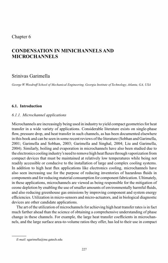
Kandlikar I044527-Ch06.tex 26/10/2005 18: 15 Page 227
Chapter 6
CONDENSATION IN MINICHANNELS ANDMICROCHANNELS
Srinivas Garimella
George W. Woodruff School of Mechanical Engineering, Georgia Institute of Technology, Atlanta, GA, USA
6.1. Introduction
6.1.1. Microchannel applications
Microchannels are increasingly being used in industry to yield compact geometries for heattransfer in a wide variety of applications. Considerable literature exists on single-phaseflow, pressure drop, and heat transfer in such channels, as has been documented elsewherein this book and can be seen in some recent reviews of the literature (Sobhan and Garimella,2001; Garimella and Sobhan, 2003; Garimella and Singhal, 2004; Liu and Garimella,2004). Similarly, boiling and evaporation in microchannels have also been studied due tothe electronics cooling industry’s need to remove high heat fluxes through vaporization fromcompact devices that must be maintained at relatively low temperatures while being notreadily accessible or conducive to the installation of large and complex cooling systems.In addition to high heat flux applications like electronics cooling, microchannels havealso seen increasing use for the purpose of reducing inventories of hazardous fluids incomponents and for reducing material consumption for component fabrication. Ultimately,in these applications, microchannels are viewed as being responsible for the mitigation ofozone depletion by enabling the use of smaller amounts of environmentally harmful fluids,and also reducing greenhouse gas emissions by improving component and system energyefficiencies. Utilization in micro-sensors and micro-actuators, and in biological diagnosticdevices are other candidate applications.
The art of the utilization of microchannels for achieving high heat transfer rates is in factmuch farther ahead than the science of obtaining a comprehensive understanding of phasechange in these channels. For example, the large heat transfer coefficients in microchan-nels, and the large surface area-to-volume ratios they offer, has led to their use in compact
E-mail: [email protected]
227
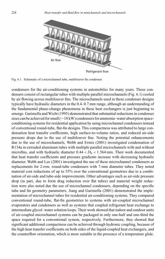
Kandlikar I044527-Ch06.tex 26/10/2005 18: 15 Page 228
228 Heat transfer and fluid flow in minichannels and microchannels
Air flow
Refrigerant flow
Fig. 6.1. Schematic of a microchannel tube, multilouver fin condenser.
condensers for the air-conditioning systems in automobiles for many years. These con-densers consist of rectangular tubes with multiple parallel microchannels (Fig. 6.1) cooledby air flowing across multilouver fins. The microchannels used in these condenser designstypically have hydraulic diameters in the 0.4–0.7 mm range, although an understanding ofthe fundamental phase-change phenomena in these heat exchangers is just beginning toemerge. Garimella and Wicht (1995) demonstrated that substantial reductions in condensersizes can be achieved for small (∼18 kW) condensers for ammonia–water absorption space-conditioning systems for residential application by using microchannel condensers insteadof conventional round-tube, flat-fin designs. This compactness was attributed to large con-densation heat transfer coefficients, high surface-to-volume ratios, and reduced air-sidepressure drops due to the use of multilouver fins. Noting the potential enhancementsdue to the use of microchannels, Webb and Ermis (2001) investigated condensation ofR134a in extruded aluminum tubes with multiple parallel microchannels with and withoutmicrofins, and with hydraulic diameter 0.44<Dh < 1.564 mm. Their work documentedthat heat transfer coefficients and pressure gradients increase with decreasing hydraulicdiameter. Webb and Lee (2001) investigated the use of these microchannel condensers asreplacements for 2-row, round-tube condensers with 7-mm diameter tubes. They notedmaterial cost reductions of up to 55% over the conventional geometries due to a combi-nation of air-side and tube-side improvements. Other advantages such as air-side pressuredrop (in part, due to form drag reduction over flat tubes) and material weight reduc-tion were also noted due the use of microchannel condensers, depending on the specifictube and fin geometry parameters. Jiang and Garimella (2001) demonstrated the imple-mentation of microchannel tubes for residential air-conditioning systems. They comparedconventional round-tube, flat-fin geometries to systems with air-coupled microchannelevaporators and condensers as well as systems that coupled refrigerant heat exchange tointermediate glycol–water solution loops. Their work showed that indoor and outdoor unitsof air-coupled microchannel systems can be packaged in only one-half and one-third thespace required for a conventional system, respectively. Furthermore, they showed thatsignificant additional compactness can be achieved through hydronic coupling, because ofthe high heat transfer coefficients on both sides of the liquid-coupled heat exchangers, andthe counterflow orientation, which is more suitable in the presence of a temperature glide.

Kandlikar I044527-Ch06.tex 26/10/2005 18: 15 Page 229
Chapter 6. Condensation in minichannels and microchannels 229
It was also shown that the refrigerant charge of the microchannel air-coupled system is20% less than that of the round-tube heat pump. For the hydronically coupled system, therefrigerant charge is only 10% of the charge in the round-tube heat pump, yielding signifi-cant benefits pertaining to the reduction of the environmental impact of air-conditioningsystems. These representative studies clearly demonstrate the wide-ranging benefits thatcan be obtained by the use of microchannels in phase-change applications.
6.1.2. Microchannel phenomena
Researchers have discussed the term “microchannel” at some length in the literature andelsewhere in this book. One extreme of the size range (sub-micron size channels) is wherecontinuum phenomena do not apply, and properties such as viscosity, ice point, and otherschange due to molecular and electrokinetic forces, but not much information is availablefor that size range, and there are few practical phase-change applications at that range.However, such non-continuum phenomena do not have to be present for there to be differ-ences in flow and heat transfer phenomena from conventional, larger diameter channels.One simple way of looking at microchannels is the existence of deviations in pressuregradients and heat transfer coefficients from widely available models, which is sufficientto warrant studies that understand and account for the different flow phenomena. In boilingapplications, for example, the microchannel designation may be applied when the chan-nel size approaches the bubble departure diameter, which would lead to differences frommacrochannel phenomena. Essentially, when channel size affects flow, pressure gradientsand heat transfer in a manner that are not accounted for by models developed for the largerchannels, it warrants a different treatment. Thus, microchannel phase change differs fromits counterpart in macrochannels due to differences in the relative influences of gravity(whose effects are less prominent at small scales), shear, and surface tension, the latterplaying a dominant role. The microchannel behavior, therefore, depends on phenomenathat do not exist or are not prominent at the larger scales, or phenomena that are suppressedat the small scales. As these phenomena would depend on the liquid and vapor phase prop-erties of the fluid under consideration, a rigorous definition of the term microchannelwould necessarily depend on the fluid in question. Serizawa et al. (2002), who conductedair–water and steam–water flow visualization studies in 50-µm channels, recommend theLaplace constant L>Dh (also referred to as the capillary length scale) as the criterion fordetermining whether a channel should be considered to be a microchannel:
L =√
σ
g (ρl − ρv)(6.1)
The Laplace constant represents the ratio of surface tension and gravity forces, and has beeninterpreted as the dimension at which influence of surface tension becomes more importantthan the stratifying effect of gravity (Fukano and Kariyasaki, 1993). This criterion impliesthat for a high surface tension fluid pair like air–water at standard temperature and pres-sure, a channel with Dh < 2.7 mm would be a microchannel, while for R-134a at 1500 kPa,the corresponding value is Dh < 0.66 mm. Another interpretation of a different form ofthis same quantity is provided in terms of the confinement of bubbles in channels (Kew
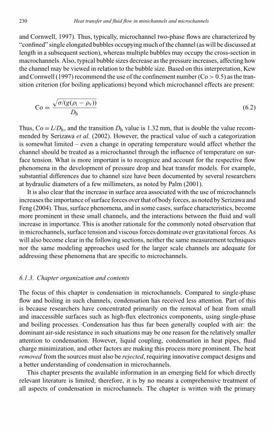
Kandlikar I044527-Ch06.tex 26/10/2005 18: 15 Page 230
230 Heat transfer and fluid flow in minichannels and microchannels
and Cornwell, 1997). Thus, typically, microchannel two-phase flows are characterized by“confined” single elongated bubbles occupying much of the channel (as will be discussed atlength in a subsequent section), whereas multiple bubbles may occupy the cross-section inmacrochannels. Also, typical bubble sizes decrease as the pressure increases, affecting howthe channel may be viewed in relation to the bubble size. Based on this interpretation, Kewand Cornwell (1997) recommend the use of the confinement number (Co> 0.5) as the tran-sition criterion (for boiling applications) beyond which microchannel effects are present:
Co =√σ/(g(ρl − ρv))
Dh(6.2)
Thus, Co = L/Dh, and the transition Dh value is 1.32 mm, that is double the value recom-mended by Serizawa et al. (2002). However, the practical value of such a categorizationis somewhat limited – even a change in operating temperature would affect whether thechannel should be treated as a microchannel through the influence of temperature on sur-face tension. What is more important is to recognize and account for the respective flowphenomena in the development of pressure drop and heat transfer models. For example,substantial differences due to channel size have been documented by several researchersat hydraulic diameters of a few millimeters, as noted by Palm (2001).
It is also clear that the increase in surface area associated with the use of microchannelsincreases the importance of surface forces over that of body forces, as noted by Serizawa andFeng (2004). Thus, surface phenomena, and in some cases, surface characteristics, becomemore prominent in these small channels, and the interactions between the fluid and wallincrease in importance. This is another rationale for the commonly noted observation thatin microchannels, surface tension and viscous forces dominate over gravitational forces. Aswill also become clear in the following sections, neither the same measurement techniquesnor the same modeling approaches used for the larger scale channels are adequate foraddressing these phenomena that are specific to microchannels.
6.1.3. Chapter organization and contents
The focus of this chapter is condensation in microchannels. Compared to single-phaseflow and boiling in such channels, condensation has received less attention. Part of thisis because researchers have concentrated primarily on the removal of heat from smalland inaccessible surfaces such as high-flux electronics components, using single-phaseand boiling processes. Condensation has thus far been generally coupled with air: thedominant air-side resistance in such situations may be one reason for the relatively smallerattention to condensation. However, liquid coupling, condensation in heat pipes, fluidcharge minimization, and other factors are making this process more prominent. The heatremoved from the sources must also be rejected, requiring innovative compact designs anda better understanding of condensation in microchannels.
This chapter presents the available information in an emerging field for which directlyrelevant literature is limited; therefore, it is by no means a comprehensive treatment ofall aspects of condensation in microchannels. The chapter is written with the primary

Kandlikar I044527-Ch06.tex 26/10/2005 18: 15 Page 231
Chapter 6. Condensation in minichannels and microchannels 231
application of refrigerant condensation and condensers as the basis, but can be extendedas necessary to other related applications. Heat transfer coefficients and pressure drops forcondensation inside microchannels are strongly dependent on the different flow patternsthat are established as the fluid undergoes a transition from vapor to liquid. Methods topredict flow regimes as a function of flow-related parameters such as mass flux, quality,and fluid properties are therefore presented first. Where possible, the differences betweenthe flow patterns in large channels and microchannels are discussed. This is followed by abrief discussion of void fraction in condensing flows. The void fraction is almost invariablyrequired for the modeling of pressure drop and heat transfer in two-phase flow. (Once again,it is noted that void fractions in microchannels have proved to be difficult to measure due toissues such as optical access, and the dynamic and sometimes indeterminate nature of thevapor–liquid interface.) Models for the prediction of pressure drops in the different flowregimes are then presented along with a comparison of the predicted pressure drops fromthe different models. This is followed by a presentation of the corresponding models forcondensation heat transfer in microchannels. Finally, areas of critical research needs forfurthering the understanding of condensation in microchannels are pointed out. At the timeof this writing, there is ongoing research in this field at several laboratories around the world,and the information presented here will no doubt need to be updated on a continuous basis.
6.2. Flow regimes
The first step in understanding condensation in microchannels is the characterization ofhow the condensing fluid flows through the channels, because this forms the basis forthe associated pressure drop and heat transfer. As the fluid condenses in the channel andprogresses from the vapor phase toward the liquid phase over a range of qualities, dif-ferent flow patterns are established at different regions of the condenser. The progressionof flow regimes, and in particular, the transitions between the different flow mechanisms,is different in microchannels than those in larger diameter tubes, primarily due to dif-ferences in relative magnitudes of gravity, shear, viscous, and surface tension forces.Similar differences exist between flow regimes and transitions in circular and non-circularmicrochannels. Therefore, extrapolation of large round-tube correlations to smaller diame-ters and non-circular geometries could introduce errors into pressure drop and heat transferpredictions. Also, the design of optimal condensers often requires the provision of vary-ing tube-side flow area. If a constant tube-side cross-sectional area is provided, the highvelocities in the initial portion of the condenser would result in excessive pressure dropswith a corresponding decrease in saturation temperature and driving temperature differ-ence, while the low velocities toward the end of the condenser would result in very lowheat transfer coefficients. A gradually decreasing flow cross-section through the use ofvarying numbers of tubes per pass is therefore desirable for optimal condenser design. Theselection of tube sizes and pass arrangements for a given application would require not justan average condensation coefficient, but rather an understanding of the variation in heattransfer coefficient and pressure drop with quality, phase velocities, and flow patterns.
Unfortunately, the bulk of the literature on two-phase flow regimes is on adiabatic flows,in which air–water, nitrogen–water, and air–oil mixtures, typically in the absence of heat
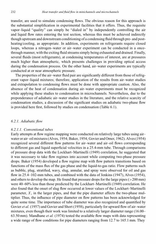
Kandlikar I044527-Ch06.tex 26/10/2005 18: 15 Page 232
232 Heat transfer and fluid flow in minichannels and microchannels
transfer, are used to simulate condensing flows. The obvious reason for this approach isthe substantial simplification in experimental facilities that it offers. Thus, the requisitevapor–liquid “quality” can simply be “dialed in” by independently controlling the airand liquid flow rates entering the test section, whereas this must be achieved indirectlythough upstream and downstream conditioning of a condensing fluid through pre- and post-heating/cooling, as appropriate. In addition, experiments on refrigerants require closedloops, whereas a nitrogen–water or air–water experiment can be conducted in a once-through manner, with the exiting fluid streams simply being exhausted and drained. Finally,several fluids (most refrigerants), at condensing temperatures of interest, are at pressuresmuch higher than atmospheric, which presents challenges in providing optical accessduring the condensation process. On the other hand, air–water experiments are typicallyconducted at or near atmospheric pressure.
The properties of the air–water fluid pair are significantly different from those of refrig-erant vapor–liquid mixtures; therefore, application of the results from air–water studiesand extrapolation to condensing flows must be done with appropriate caution. Also, theabsence of the heat of condensation during air–water experiments must be recognizedwhile applying these studies to condensation in microchannels. Nevertheless, due to thepreponderance of adiabatic air–water studies in the literature, and the relative scarcity ofcondensation studies, a discussion of the significant studies on adiabatic two-phase flowis provided here first, followed by studies on condensation (Table 6.1).
6.2.1. Adiabatic flow
6.2.1.1. Conventional tubesEarly attempts at flow regime mapping were conducted on relatively large tubes using air–water or air–oil mixtures (Alves, 1954; Baker, 1954; Govier and Omer, 1962). Alves (1954)recognized several different flow patterns for air–water and air–oil flows correspondingto different gas and liquid superficial velocities in a 25.4-mm tube. Through comparisonsof pressure drop data with the Lockhart–Martinelli (1949) correlation, he suggested thatit was necessary to take flow regimes into account while computing two-phase pressuredrops. Baker (1954) developed a flow regime map with flow pattern transitions based onfunctions of the mass flux of the gas phase and the liquid-to-gas ratio. Flow patterns suchas bubble, plug, stratified, wavy, slug, annular, and spray were observed for oil and gasflow in 25.4–102-mm tubes, and combined with the data of Jenkins (1947), Alves (1954),and others to develop the map. He found that pressure drops for the large pipes (>200 mm)were 40–60% less than those predicted by the Lockhart–Martinelli (1949) correlation. Healso found that the onset of slug flow occurred at lower values of the Lockhart–Martinelliparameter, X , in the larger pipes, and that the pipe diameter affects the two-phase mul-tiplier. Thus, the influence of pipe diameter on flow patterns has been acknowledged forquite some time. The importance of tube diameter was also recognized and quantified byGovier et al. (1957) and Govier and Short (1958), particularly for upward flow of air–watermixtures, even though their work was limited to a relatively larger diameter range (16.00–63.50 mm). Mandhane et al. (1974) tested the available flow maps with data representinga wide range of flow conditions for pipe diameters ranging from 12.7 to 165.1 mm. They

Kandlikar
I044527-Ch06.tex
26/10/200518:15
Page233
Table 6.1Summary of flow regime studies.
Hydraulic Orientation/ Range/Investigators diameter Fluids conditions applicability Techniques, basis, observations
Adiabatic flow: conventional tubesTaitel and Air–water • Devised theoretical approach to flow regime mapping usingDukler (1976) a momentum balance on a stratified flow pattern
Mandhane 12.7–165.1 mm Air–water Horizontal 0.043< jG < 170.7 m/s • “Best fit” map from available flow regime mapset al. (1974) 0< jL < 7.315 m/s • Introduced physical property corrections
Adiabatic flow: small circular channelsSuo and Griffith 1–6 mm Air–water Horizontal ρl/ρg >> 1 • Transition from elongated bubble to annular and bubbly flow(1964) adiabatic µl/µg > 25 • Criterion to determine when buoyancy effects can be neglected
Barnea et al. 4–12 mm Air–water Horizontal T = 25◦C • Recommended Taitel and Dukler (1976) model for all(1983) Pexit = 1 atm transitions except stratified to non-stratified
0.001< jL < 10 m/s • Modified stratified-to-intermittent transition boundary of Taitel0.01< jG < 100 m/s and Dukler (1976)
Damianides 1–5 mm Air–water Horizontal P ∼ 5 atm • Documented effect of hydraulic diameterand Westwater T ∼ 15–20◦C • Some agreement for 5 mm with Taitel and Dukler (1976), but(1988) 0.001< jL < 10 m/s poor agreement for 1 mm
0.01< jG < 100 m/s • 1-mm tube showed large intermittent flow region• Increasingly small stratified flow region in small diameter tubes
Fukano et al. 1–4.9 mm Air–water Horizontal Pexit = 1 atm • Results agreed with Barnea et al. (1983) but not with Damianides(1989) adiabatic 0.04< jG < 40 m/s and Westwater (1988)
0.2< jL < 4 m/s • Mandhane et al. (1974) cannot predict transitions in small tubes• Taitel and Dukler (1976) and Weisman et al. (1979) not reliable
for small diameters
Brauner and 4–25.2 mm Air–water Horizontal 0.01< jG < 40 m/s • Incorporated the stabilizing effect of surface tension associatedMaron (1992) 0.001< jL < 0.3 m/s with practically finite wavelengths
• Transition criteria based on Eotvos number
(Continued )

Kandlikar
I044527-Ch06.tex
26/10/200518:15
Page234
Table 6.1(Continued )
Hydraulic Orientation/ Range/Investigators diameter Fluids conditions applicability Techniques, basis, observations
Ide et al. (1995) 0.5–6 mm Air–water Vertical • Studied “liquid lumps” formed in vertically upward flowupwards • Velocity characteristics of liquid lumps used to interpret flow
pattern with corresponding maps by Fukano et al. (1989)
Mishima and 1–4 mm Air–Water Vertical 0.0896< jG < 79.3 m/s • Neutron radiography for flow visualization and void fractionsco-workers upwards 0.0116< jL < 1.67 m/s • Recommended transition criteria of Mishima and Ishii (1984)(Mishima and Hibiki,1996; Mishima et al.,1997; Mishimaand Hibiki, 1998)
Coleman and 5.5-, 2.6-, 1.75-, Air–water Horizontal 0.1< jG < 100 m/s • Diameter has significant effect on flow regime transitionsGarimella (1999) 1.3-mm circular 0.01< jL < 10 m/s • Intermittent flow regime increases in small diameter tubes
Dh = 5.36 mm • Comparisons with the criteria of Damianides and Westwater(α= 0.725) (1988), Fukano et al. (1989) and Weisman et al. (1979)rectangular
Triplett et al. 1.1- and 1.45-mm Air–water Horizontal 0.02< jG < 80 m/s • Observed bubbly, churn, slug, slug-annular and annular flow(1999b) circular; adiabatic 0.02< jL < 8 m/s • No stratified flow
semi-triangular • Maps agreed with Damianides and Westwater (1988),1.09 and 1.49 mm Fukano et al. (1989) and Fukano and Kariyasaki (1993)
• Poor agreement with analytically derived criteria(Suo and Griffith, 1964; Taitel and Dukler, 1976)
Zhao and Bi Triangular channels Air–water Vertical 0.1< jG < 100 m/s; • Dispersed bubbly flow not observed in smallest channel,(2001a) Dh = 2.886, 1.443, upward For Dh = 2.886, 1.443 but capillary bubble flow pattern seen
and 0.866 mm 0.08< jL < 6 m/s • Trends agreed well with several investigators (Barnea et al.,For Dh = 0.866 1983; Galbiati and Andreini, 1992a; Mishima and Hibiki, 1996;0.1< jL < 10 m/s Ide et al., 1997), but not with Taitel and Dukler (1976)
and Mishima and Ishii (1984)
Yang and 1, 2, and 3 mm Air–water Horizontal T = 25–30◦C • Transitions difficult to distinguish for air–water, but clearShieh (2001) adiabatic 0.016< jG < 91.5 m/s for R-134a
0.006< jL < 2.1 m/s • Lower σ of R-134a compared to air–water led to differencesR-134a 300<G< 1600 kg/m2-s • R-134a transitions agreed with Hashizume (1983) and
T = 30◦C Wang et al. (1997a)

Kandlikar
I044527-Ch06.tex
26/10/200518:15
Page235
Tabatabai and 4.8–15.88-mm Water Horizontal • Flow regime maps based on relative effects ofFaghri (2001) condensation R-12 surface tension, shear, and buoyancy forces
12.3–1-mm R-113 • Better agreement with available data in shear-dominated regionsair–water R-22 • Predicts movement of boundaries with channel size
R-134a
Adiabatic flow: narrow, high-aspect ratio, rectangular channelsTroniewski and Rectangular Air–water Horizontal T = 25–35◦C • Corrections to axes of Baker (1954) map based on single-phaseUlbrich (1984) 0.09<α< 10.10 0.6< jG < 43 m/s velocity profiles
7.45<Dh < 13.1 200< jL < 1600 m/sVertical T = 25–35◦C
0.7<µL < 40 × 10−3 Pa s995<ρL < 1150 kg/m3
Wambsganss Rectangular Air–water Horizontal 0.0001< x< 1 • Flow visualization and dynamic pressure measurementset al. (1991; α= 6, 0.167 adiabatic 50<G< 2000 kg/m2-s • Qualitative agreement with large circular channels but
1994) Dh = 5.44 mm quantitative differences• Transition criteria for bubble or plug flow to slug flow
based on root-mean-square pressure changes
Xu and Rectangular Air–water Vertical Pexit = 1 atm • Bubbly, slug, churn, and annular flow in 0.6- and 1-mm channelsco-workers gap = 0.3, adiabatic 0.01< jG < 10 m/s • Bubbly flow absent in 0.3-mm channel(Xu, 1999; 0.6, and 1 mm 0.01< jL < 10 m/s • Extended criteria of Mishima and Ishii (1984) for applicationXu et al., 1999) to narrow rectangular geometry
Hibiki and Rectangular Air–water, Vertical Air–water data • Criteria specifically for narrow rectangular channelsMishima (2001) channels with steam–water upward (from Sadatomi et al., based on Mishima and Ishii (1984) criteria
gap 0.3–17 mm 1982; Lowry and Kawaji, • Collision/coalescence of bubbles increase when maximum1988; Ali et al., 1993; distance between bubbles < projected bubble diameterMishima et al., 1993;Wilmarth and Ishii,1994; Xu, 1999)Steam–water data(from Hosler, 1968)
(Continued )

Kandlikar
I044527-Ch06.tex
26/10/200518:15
Page236
Table 6.1(Continued )
Hydraulic Orientation/ Range/Investigators diameter Fluids conditions applicability Techniques, basis, observations
Adiabatic flow: microgravityRezkallah et al. 9.525 mm Air–water Microgravity 0.09< jG < 30 m/s • Slug at µg different from “Taylor bubble” profile seen at 1-g(Rezkallah, 1995; Air–glycerin/ 0.015< jL < 3.5 m/s • Annular flow regime similar to 1-gRezkallah and water 0.6< jG < 12 m/s • Little effect of µL on transitionsZhao, 1995; 0.7< jL < 2 m/s • Later verified and modified based on 6–40-mm tubesLowe andRezkallah, 1999)
Adiabatic flow: D << 1 mmKawahara 100 µm Nitrogen–water Horizontal 0.1< jG < 60 m/s • Low Re at small Dh implies greater effects of wall shear andet al. 0.02< jL < 4 m/s surface tension(2002) • Observed liquid slug, gas core with smooth-thin liquid film,
gas core with smooth-thick liquid film, gas core withring-shaped liquid film, and gas core with deformed interface
• No gravitational effects, absence of bubbly flow (no bubblebreakup due to absence of liquid phase turbulence at low Re)
• Flow conditions determine likely, but not unique patterns• Map based on probability of occurrence of patterns• Four flow regimes (slug-ring, ring-slug, semi-annular, and
multiple), which are combinations of flow mechanisms
Chung and 530, 250, 100, Nitrogen–water Horizontal 0.02< jG < 73 m/s • Extended work of Kawahara et al. (2002) for effect of diameterKawaji and 50 µm 0.01< jL < 5.77 m/s • 530- and 250-µm flow similar to ∼1-mm flow(2004) • Slug flow in small channels; absence of bubbly, churn,
slug-annular, and annular flow
Chung 96-µm square Nitrogen–water Horizontal Circular data • Negligible effect of channel shapeet al. 100-µm circular (from Chung and(2004) Kawaji, 2004)
Serizawa 20-, 25-, and Air–water, steam Horizontal 0.0012< jG < 295.3 m/s • Results different from other investigators of D<< 1-mm channelset al. (2002) 100-µm (only 50 µm) 0.003< jL < 17.52 m/s • Numerous terms to define flow patterns
circular • Bubbly flow in 25-µm channel

Kandlikar
I044527-Ch06.tex
26/10/200518:15
Page237
• High capillary pressure at small bubble interface keeps bubblespherical and prevents coalescence
• Slug flow due to entrance phenomenon, not bubble coalescence• Liquid ring flow due to rupture of liquid bridges between
bubbles at high gas velocities• Surface tension prevents liquid slugs from spreading as film,
leads to dry patches, liquid “lumps”• State that air–water and steam–water patterns in 25-µm channel
similar; photographs presented seem dissimilar• Surprisingly state that flow map agrees with large channel
Mandhane et al. (1974) map, but graphs indicate otherwise
Condensing flowTraviss and 8 mm R-12 Horizontal 100<G< 990 kg/m2-s • Disperse, annular, semi-annular, and slug flow observedRohsenow condensing 10<T < 40.6◦C • Froude number as basis for condensation mode(1973) • von Karman velocity profile to describe film velocity
Breber 4.8–50.8 mm R-11, R-12, Horizontal 108.2<P< 1250 kPa • Taitel and Dukler (1976) map to develop simple criteria foret al. (1980) R-113, steam, condensing 17.6<G< 990 kg/m2-s condensation in horizontal tubes
n-pentane • Criteria based on ratio of shear to gravity forces• All map boundaries vertical and horizontal lines – easy to use• Defined transition regions, rather than abrupt transitions
Sardesai 24.4 mm R-113, steam, Horizontal • Investigated annular–stratified/wavy transitionet al. (1981) propane, condensing • Taitel and Dukler (1976) annular–stratified/wavy transition
methanol, criterion as basis to develop transition criterion from datan-pentane
Soliman 4.8<D< 15.9 mm R-12, Condensing • Annular–wavy Froude number transition criterion based on(1982; 1986) R-113, steam data from different sources
• Mist–annular Weber number transition criterionTandon et al. 4.8<D< 15.9 mm R-12, Condensing 0.01< j∗g < 20 • Simple transition criteria, good agreement with data(1982; 1985a) R-113, R-22 0.001 < 1 − α/α< 3 for annular, semi-annular, and wavy flows
Hashizume et al. 10 mm R-12, R-22 Horizontal 570< p< 1960 kPa • Refrigerant flow patterns different from air–water(Hashizume, 1983; condensing • Modified property corrections of Baker (1954)Hashizume et al., map proposed by Weisman et al. (1979) to make1985; Hashizume them applicable to R-12 and R-22and Ogawa, 1987)
(Continued )

Kandlikar
I044527-Ch06.tex
26/10/200518:15
Page238
Table 6.1(Continued )
Hydraulic Orientation/ Range/Investigators diameter Fluids conditions applicability Techniques, basis, observations
Wang et al. 6.5 mm R-22, R-134a, Horizontal 50<G< 700 kg/m2-s • At low G, intermittent and stratified flow;(1997a, b) R-407C Tsat = 2, 6, and 20◦C at high G, annular
• Agreed with modified Baker (1954) map ofHashizume et al. (Hashizume, 1983; Hashizume et al.,1985; Hashizume and Ogawa, 1987)
Dobson and 3.14, 4.6, R-12, Horizontal Condensing • Good agreement with Mandhane et al. (1974) map afterco-workers and R-134a, 25<G< 800 kg/m2-s axis transformation(Dobson, 1994; 7.04 mm R-22, T = 35–60◦C • Primary distinction between gravity and shear-controlledDobson et al., R32/R125 flows1994; Dobson • Criteria based on modified Soliman number and mass fluxand Chato, 1998)
Coleman and Round: 4.91 mm; R-134a Horizontal P = 1379–1724 kPa • Flow regimes subdivided into flow patterns, G–x basedGarimella Square: 4, 3, condensing 150<G< 750 kg/m2-s transition criteria(2000 a, b; 2003), 2, 1 mm; • Dh more important than shape, aspect ratio for transitionGarimella (2004) Rectangular: criteria
4 × 6; 6 × 4; • Intermittent and annular flow increases as Dh decreases2 × 4; 4 × 2 mm • Wavy flow non-existent in 1-mm channel
Cavallini et al. 8 mm R-22, Condensation, 30<Tsat < 50◦C • Criteria similar to Breber et al. (1979; 1980) for primary(2001; 2002a, b) R-134a, R-125, horizontal 100<G< 750 kg/m2-s flow regimes (annular, stratified, wavy, and slug)
R-32, R-236ea, tubes • Recommended Kosky and Staub (1971) model forR-407C, annular flowand R-410A
El Hajal 3.14<D< 21.4 mm R-22, R-134a, Horizontal 16<G< 1532 kg/m2-s • Transitions between stratified, wavy, intermittent, annular,et al. (2003) R-125, R-32, condensing 0.02< pr < 0.8 mist and bubbly flow on G–x coordinates, adapting
R-236ea, R-410a 76< (We/Fr)L < 884 boiling map of Kattan et al. (1998a, b; 1998c) withupdates by Zurcher et al. (1999)
• Void fraction for map construction deduced from heattransfer database, subsequently averaged withhomogeneous value

Kandlikar I044527-Ch06.tex 26/10/2005 18: 15 Page 239
Chapter 6. Condensation in minichannels and microchannels 239
developed a “best fit” map from the different flow regime maps available at the time, andalso introduced physical property corrections for gas and liquid density, gas and liquid vis-cosity, and surface tension to be applied to the transition lines. However, these correctionsdid not yield a significant improvement in flow pattern prediction. A theoretical modelof pressure drop for slug flows in horizontal and near-horizontal tubes was developed byDukler and Hubbard (1975) with the two main contributions to pressure drop being theacceleration of the liquid to the slug velocity, and the pressure drop due to wall shear at theback of the slug. This model was validated using pressure–time traces and individual phasevelocity measurements. Nicholson et al. (1978) extended this model to include elongatedbubble flows by using a constant slug length, and also used the model to predict flow regimetransitions. Taitel and Dukler (1976) devised a theoretical approach to flow regime map-ping for air–water mixtures using a momentum balance on a stratified flow pattern. A setof four non-dimensional parameters was used to define instability-driven transitions fromthe stratified to annular or intermittent flows, and to distinguish between stratified smoothand stratified wavy flows. This theoretical model showed good agreement with the exper-imentally developed flow map of Mandhane et al. (1974). The effects of fluid properties(liquid viscosity, surface tension, gas density) and pipe diameter on two-phase horizontalflow patterns were investigated by Weisman et al. (1979) for pipe diameters ranging from11.5 mm to 51 mm. Using data from other investigators as well as new flow visualizationand pressure fluctuation data, modifications to existing correlations were developed forthe flow-regime transitions. It was concluded that for the range of diameters tested, thepipe diameters and fluid properties have only moderate influences on the transition lines.
Some investigators (Moore and Turley, 1983; Cai et al., 1996) have used statisticalapproaches to better define the transitions between flow regimes (plug or bubble to slugflow, annular to annular–mist flow) that are difficult to distinguish visually. This approachutilizes the root mean square and fluctuations in the pressure/time signals, frictional pres-sure gradients, and chaos theory to provide an objective means to interpret flow patterntransitions. Annunziato and Girardi (1987) used differential pressure measurement andlocal void fraction probes to measure the temporal fluctuations in a 89-mm diameter tube.
6.2.1.2. Small circular channelsAmong the studies on flow regime maps for microchannels using adiabatic air–watermixtures, Suo and Griffith (1964) correlated the transition from elongated bubble to annularand bubbly flow in capillary tubes (1.0<D< 1.6 mm) by using the average volumetricflows of the liquid and gas phases, and the velocity of the bubbles. They also provideda criterion which determines when buoyancy effects can be neglected in terms of theparameter ρlgD2/σ. However, it must be noted that they restrict their analysis to situationswhereρl/ρg � 1 andµl/µg > 25. While they explicitly state these restrictions in their paper,several other air–water adiabatic flow papers do not establish such explicit restrictions;therefore, caution is advised when applying these air–water based criteria to refrigerantcondensation. For example, for refrigerant R-134a condensing at 1500 kPa, the densityratio is 14, while the viscosity ratio is 9.7. For the air–water pair at standard conditions,the corresponding ratios are ρl/ρg = 839 and µl/µg = 49. Similarly, the surface tension ofthe air–water pair is 17 times higher than that of R-134a.

Kandlikar I044527-Ch06.tex 26/10/2005 18: 15 Page 240
240 Heat transfer and fluid flow in minichannels and microchannels
Barnea et al. (1983) classified two-phase flow patterns in small horizontal tubes(4<D< 12 mm) into to four major regimes (dispersed, annular, intermittent and strat-ified). They found that all transitions except the stratified to non-stratified transition weresatisfactorily described by the Taitel–Dukler (1976) model. Therefore, they modified thestratified-to-intermittent flow transition boundary predicted by Taitel and Dukler (1976) byaccounting for surface tension in terms of the gas-phase height in the channel as follows:
hG ≤ π
4
√σ
ρg(1 − π
4
) (6.3)
Even though the above equation includes surface tension and gravitational terms, theycommented that for small channels, this condition is always satisfied, which leads toa further simplification of the criterion, namely, hG ≤ π
4 D. They also provided differentinterpretations for the formation of intermittent flow from stratified flows. In large channels,they attribute the transition to the Kelvin–Helmholtz instability, whereas in small tubeswith wetting liquid, wetting of the wall due to capillary forces causes the film to climb andform a bridge, which leads to intermittent flow.
Damianides and Westwater (1988) developed individual flow regime maps for air–water mixtures for 1<Dh < 5 mm to document the effect of diameter on the flow regimetransitions. They found some agreement between their results and the transition criteria ofTaitel and Dukler (1976) for the 5-mm case, but the agreement was poor for 1-mm tubes.The 1-mm tube showed a large intermittent flow region, with the transition from annularflow attributed to the generation of roll waves. For the larger diameter tubes, they reportedthe existence of an increasingly large region of stratified wavy flow, with the waves creepingup to form annular flow at larger gas velocities. The agglomeration of plugs of gas led toslug flow, rather than the growth of a finite amplitude wave, which meant that the Kelvin–Helmholtz instability could not be used to predict the onset of slugging. As observed byalmost all investigators, they also stated increasingly important role of surface tension atthe smaller channel diameters. They noted that the intermittent-to-disperse flow transitionoccurred at larger liquid flow rates in the larger tubes, and that the intermittent-to-annulartransition occurred at larger gas flow rates in smaller tubes. The stratified flow region wasessentially non-existent in the 1-mm tube.
Fukano et al. (1989) also investigated air–water flow patterns in tubes with1<Dh < 4.9 mm and recorded bubbly, annular, plug, and slug flows, the latter two beingcombined into one intermittent region for pressure drop analyses. Their results agreedwith the work of Barnea et al. (1983), and while there is some disagreement betweenthe results reported by Fukano et al. (1989) and Damianides and Westwater (1988), thesestudies do point out that the flow regime map presented by Mandhane et al. (1974) cannotsufficiently predict the flow regime transitions in small diameter tubes. Also, it appearsthat the theoretical predictions of Taitel and Dukler (1976) and the correlations presentedby Weisman et al. (1979) are not reliable for small diameters.
Brauner and Maron (1992) noted that several previous researchers had based their flowregime transition analyses on single stability criteria of infinitely long waves. Therefore,they incorporated the stabilizing effects of surface tension associated with practically finite

Kandlikar I044527-Ch06.tex 26/10/2005 18: 15 Page 241
Chapter 6. Condensation in minichannels and microchannels 241
wavelengths, and were able to predict the transition from stratified flow over a wide rangeof channel sizes. This resulted in a transition criterion based on the Eotvos number:
Eo = (2π)2 σ(ρl − ρg
)D2g
> 1 (6.4)
Ide et al. (1995) studied the “liquid lumps” formed during vertical upward air–water flowin six tubes with 0.5<D< 6.0 mm, including the velocity of the lumps, the correspondingdisturbance wave and the base film. A momentum-averaged mean velocity of liquid lumpswas used to characterize the flow for cases with large liquid lumps and many small waves.The liquid lump velocity characteristics were then used to interpret the flow patterns withcorresponding maps (Fukano et al., 1989) for horizontal capillary tubes.
Mishima and Hibiki (1996) investigated flow patterns for upward flow of air–watermixtures in vertical tubes (an orientation that is not particularly relevant for condensationapplications) with 1<D< 4 mm. Some variants of flow patterns typically seen in largertubes were observed, but the transitions were in reasonable agreement with Mishima andIshii’s (1984) transition criteria. Mishima et al. (1997; 1998) used neutron radiography,which uses the fact that thermal neutrons easily penetrate heavy materials such as metals,but are attenuated by light materials containing hydrogen, that is water, to non-intrusivelyinvestigate qualitative and quantitative two-phase flow phenomena. Thus, the incidentneutron beam is attenuated in proportion to the liquid phase thickness, allowing projectionof the image of the two-phase flow, which is then converted to an optical image by thescintillator. The image is intensified and enlarged, and detected by a high-speed videocamera. Air–water vertical upward flow was visualized to identify the prevailing flowregime, rising velocity of bubbles, and wave height and interfacial area in annular flow.Representative images of slug flow before and after processing are shown in Fig. 6.2. Voidprofiles and void fraction variations were also recorded as discussed in a subsequent section.By utilizing attenuation characteristics of neutrons in materials, measurements of voidprofile and average void fraction were performed. This technique enables flow visualizationin situations without optical access and where X-ray radiography is not applicable.
Coleman and Garimella (1999) investigated the effect of tube diameter and shape onflow patterns and flow regime transitions for air–water flow in circular tubes of 5.5-, 2.6-,1.75-, and 1.3-mm diameter, and a rectangular tube with Dh = 5.36 mm and aspect ratioα= 0.725. Gas and liquid superficial velocities were varied from 0.1 m/s<USG < 100 m/s,and 0.01 m/s<USL < 10.0 m/s, respectively. Bubble, dispersed, elongated bubble, slug,stratified, wavy, annular–wavy, and annular flow patterns were observed (Fig. 6.3). Thisfigure also shows their attempt to bring some uniformity to the terminology used to describethese flow mechanisms by the various investigators cited above. Thus, they divided themechanisms into four major regimes (stratified, intermittent, annular, and dispersed) andsubdivided these major regimes further into the applicable patterns. Thus, when comparingwith the results of various investigators, the nomenclature for at least the major regimeswould be somewhat uniform. The tube diameter had a significant effect on the transitions.As the tube diameter is decreased, the transition from the intermittent regime to the dis-persed or bubbly regime occurred at progressively higher USL. Also, the transition fromintermittent to annular flow occurs at a nearly constant USL, for a given tube, with the

Kandlikar I044527-Ch06.tex 26/10/2005 18: 15 Page 242
242 Heat transfer and fluid flow in minichannels and microchannels
(a)
(b)
Fig. 6.2. Raw and processed images of slug flow in vertical upward air–water flow. Reprinted fromMishima, K., Hibiki, T. and Nishihara, H., Visualization and measurement of two-phase flow by using neutronradiography, Nuclear Engineering and Design, 175(1–2), pp. 25–35 (1997) with permission from Elsevier.
transition USL increasing as the diameter first decreases from 5.5 mm, but approaching alimiting value as the diameter decreases further to 1.75 and 1.30 mm. The size of the inter-mittent regime increases in small diameter tubes. The primary difference in their resultsfor round and rectangular channels of approximately the same Dh was that the rectangulartube showed a transition to disperse flows at higher USL, presumably because it is moredifficult to dislodge the liquid from the corners of the rectangular tube due to the surfacetension forces. As with other investigators, they found that very few points for the 5.5-mmtube were in the stratified regime, whereas the Taitel–Dukler (1976) criteria predicted theexistence of a stratified region for these conditions. The agreement with the intermittent-to-disperse and the annular-to-disperse transitions was somewhat better. However, theassumptions inherent in the Taitel–Dukler analyses were not considered applicable to thesmall diameter channels. The agreement with the data of Damianides and Westwater (1988)

Kandlikar I044527-Ch06.tex 26/10/2005 18: 15 Page 243
Chapter 6. Condensation in minichannels and microchannels 243
Stratified regime: wavy flow pattern
Intermittent regime: slug flow pattern
Annular regime: wavy–annular pattern
Annular regime: annular pattern
Dispersed regime: bubble flow pattern
Dispersed regime: dispersed flow pattern
Intermittent regime: elongated bubble pattern
Fig. 6.3. Air–water flow patterns in circular and rectangular tubes. Reprinted from Coleman, J. W. andGarimella, S., Characterization of two-phase flow patterns in small diameter round and rectangular tubes,International Journal of Heat & Mass Transfer, 42(15), pp. 2869–2881 (1999) with permission from Elsevier.
was much better. The transition to the dispersed region (including the effect of diameter)was also in good agreement with the results of Fukano et al. (1989). The transition cor-relations presented by Weisman et al. (1979) were only in agreement for the largest tubestudied by Coleman and Garimella, with the agreement deteriorating as Dh decreased.

Kandlikar I044527-Ch06.tex 26/10/2005 18: 15 Page 244
244 Heat transfer and fluid flow in minichannels and microchannels
Triplett et al. (1999b) conducted an investigation similar to that of Coleman andGarimella (1999) of flow regimes in adiabatic air–water flows through circular microchan-nels of 1.1- and 1.45-mm diameter, and in semi-triangular microchannels with Dh = 1.09and 1.49 mm. They identified bubbly, churn, slug, slug–annular, and annular flow patterns(stratified flow was not observed as was the case with many other investigators), and plottedthe data on gas and liquid superficial velocity axes. The progression between the respec-tive regimes as the gas and liquid velocities are changed is shown in Fig. 6.4. Bubbly flowundergoes a transition to slug flow when the gas superficial velocity UGS increases due tothe corresponding rise in the void fraction and the coalescence of bubbles. At high super-ficial liquid velocities ULS, as the overall mass flux is increased, churn flow is establisheddue to the disruption of slugs. Churn flow also occurred when large waves disrupted wavy–annular flows. Slug–annular flow is established at low UGS and ULS, and changes to annularflow when UGS increases. The flow regime maps for all channels tested were substantiallysimilar. Their maps agreed in general with the results of Damianides and Westwater (1988)and Fukano and Kariyasaki (1993), but the agreement with almost all analytically derivedtransition criteria (Suo and Griffith, 1964; Taitel and Dukler, 1976) was poor.
Zhao and Bi (2001a) investigated flow patterns for co-current upward air–water flow invertical equilateral triangular channels with Dh = 2.886, 1.443, and 0.866 mm. The flowpatterns encountered included dispersed bubbly flow, slug flow, churn flow and annularflow for Dh = 2.886 and 1.443 mm. For Dh = 0.866 mm, dispersed bubbly flow was notobserved, but a capillary bubbly flow pattern, consisting of a succession of ellipsoidalbubbles, spanned the cross-section of the channel (Fig. 6.5) at low gas flow rates. Longslugs were seen at high superficial gas velocities in the slug flow regime. Churn andannular flows occurred at higher superficial gas velocities as the channel size decreased.These trends were in agreement with the results of other investigators (Barnea et al., 1983;Galbiati andAndreini, 1992a; Mishima and Hibiki, 1996; Ide et al., 1997) for small circulartubes. However, occurrence of the churn–annular transition line at higher gas velocitieswith decreasing channel diameter did not agree with the findings of Taitel et al. (1980)and Mishima and Ishii (1984), who predicted the opposite trend for conventional tubes.The significant discrepancies between the data and the Taitel et al. and the Mishima–Ishiitransition criteria were attributed to the large difference in channel size and the meniscuseffect due to the triangular shape.
Yang and Shieh (2001) observed bubbly, plug, wavy, slug, annular, and dispersedregimes during air–water and R-134a (adiabatic) flow through 1-, 2-, and 3-mm horizontaltubes. Transitions between the regimes, especially slug-to-annular, were difficult to distin-guish in air–water flow, while all the R-134a transitions were clear. In a manner much likethe study by Coleman and Garimella (1999), they plotted their flow regime maps for thedifferent tubes versus the transition lines of Taitel and Dukler (1976), Barnea et al. (1983),and Damianides and Westwater (1988). The results were in generally good agreement withthose of the latter two investigators, but as pointed out by numerous other investigators, thestratified–intermittent transition predicted by Taitel and Dukler (1976) was not seen, due tothe inapplicability of the basis for this transition to the smaller tubes. The slug–annular tran-sition for R-134a occurred at lower gas velocities, while the intermittent–bubbly transitionoccurred at higher liquid velocities, both attributed to the lower surface tension of R-134acompared to the air–water pair. The R-134a transitions were in good agreement with the

Kandlikar I044527-Ch06.tex 26/10/2005 18: 15 Page 245
Chapter 6. Condensation in minichannels and microchannels 245
(a) ULS � 3.021 m/s, UGS � 0.083 m/s (b) ULS � 5.997 m/s, UGS � 0.396 m/s
(c) ULS � 0.213 m/s, UGS � 0.154 m/s (d) ULS � 0.608 m/s, UGS � 0.498 m/s
(e) ULS � 0.661 m/s, UGS � 6.183 m/s (f) ULS � 1.205 m/s, UGS � 4.631 m/s
(g) ULS � 0.043 m/s, UGS � 4.040 m/s (h) ULS � 0.082 m/s, UGS � 6.163 m/s
(i) ULS � 0.082 m/s, UGS � 73.30 m/s (j) ULS � 0.271 m/s, UGS � 70.42 m/s
Fig. 6.4. Flow regimes for adiabatic air–water flow through 1.09-mm circular channels. Reprinted fromTriplett, K. A., Ghiaasiaan, S. M., Abdel-Khalik, S. I. and Sadowski, D. L., Gas–liquid two-phase flowin microchannels, Part I: Two-phase flow patterns, International Journal of Multiphase Flow, 25(3),pp. 377–394 (1999) with permission from Elsevier.

Kandlikar I044527-Ch06.tex 26/10/2005 18: 15 Page 246
246 Heat transfer and fluid flow in minichannels and microchannels
Channel inner wall
Gas–wall interface
Gas–liquid interface
Liquid
A–A view
Gas
AA
Fig. 6.5. Capillary bubble in triangular channel. Reprinted from Zhao, T. S. and Bi, Q. C. Co-current air–watertwo-phase flow patterns in vertical triangular microchannels, International Journal of Multiphase Flow, 27(5),pp. 765–782 (2001) with permission from Elsevier.
results of Wang et al. (1997a) and Hashizume (1983), although these two investigationsfocused on lower mass fluxes than those studied by Yang and Shieh (2001).
Tabatabai and Faghri (2001) developed a flow regime map for microchannels withparticular attention to the influence of surface tension. They noted that in two-phase flow,ripples are generated on the annular layer with an increase in gas-phase velocity, which inturn leads to the formation of collars and bridges. They distinguish slug, plug, and bubbleregimes based on the size and gap between the bridges. As with other investigators, theystate that in large tubes, gravitational forces pull the liquid film down, preventing bridgeformation. Their map is based on the relative effects of surface tension, shear, and buoyancyforces. The map uses the ratio of pressure difference due to surface tension and that due toshear forces as one axis, while the ratio of superficial velocities VG,S/Vl,S forms the otheraxis. The void fraction model of Smith (1969) is used to compute the required vapor orgas-core flow area and interfacial surface area. The three terms in the force balance perunit length of the region of interest are given by:
Fsurface tension
L= 2σ(1 − α)0.5 (6.5)

Kandlikar I044527-Ch06.tex 26/10/2005 18: 15 Page 247
Chapter 6. Condensation in minichannels and microchannels 247
Fshear
L= πDαfl
(ρlu2
l
4
)(6.6)
Fbuoyancy
L= g
(ρl − ρg
)Ag (6.7)
where the void fraction α appears in each of the three equations above (indirectly throughthe gas phase area in the buoyancy term). This establishes a condition for the surfacetension forces being dominant:
|Fsurface tension| > |Fshear| + |Fbuoyancy| (6.8)
which then yields a criterion for the transition from surface-tension-dominated regions toshear-dominated regions:
ul < B =2σ(1 − α)0.5 − g
(ρl − ρg
)Ag(
πDαρl fl4
)
0.5
(6.9)
Relating the actual phase velocities to the corresponding superficial velocities resultsin the following form of the transition criterion:
VSG
VSL>
VSG
(1 − α)B(6.10)
For the annular-to-intermittent transition, they used the following criterion for the liquidvolume fraction m proposed by Griffith and Lee (1964), which is based on collars formingin annular flow due to instabilities at a wavelength of 5.5 × D, with the collar ultimatelyforming bridges and slugs:
m =(πr2
)2r − 4
3πr3
πr2(5.5)2r= 0.06 (6.11)
where the numerator is the total liquid volume per slug and the denominator is the totalvolume of the slug at the most unstable wavelength of 5.5. Tabatabai and Faghri comparedthis flow regime map with data in the literature for condensation of steam and refrigerantsin tubes with D> 4.8 mm, and for air–water flow in smaller diameter tubes, and stated thatbetter agreement was obtained in the surface-tension-dominated regions, and also that themap is able to predict the movement of the boundaries with channel size.
6.2.1.3. Narrow, high aspect ratio, rectangular channelsMost of the research on two-phase flow in small hydraulic diameter rectangular channelsuses tubes of either small (α< 0.50) or large (α> 2.0) aspect ratios (Hosler, 1968; Jones Jr.and Zuber, 1975; Lowry and Kawaji, 1988; Wilmarth and Ishii, 1994). In a study on flowregime maps for 0.125<α< 0.50 and 11.30<Dh < 33.90 mm, Richardson (1959) showedthat the smaller aspect ratio suppressed the stratified and wavy flow regimes and promotedthe onset of elongated bubble and slug flows. Troniewski and Ulbrich (1984) proposed
Kandlikar I044527-Ch06.tex 26/10/2005 18: 15 Page 248
248 Heat transfer and fluid flow in minichannels and microchannels
corrections to the axes of the Baker (1954) map based on the single-phase velocity profilesin rectangular channels for horizontal and vertical channels with 0.09<α< 10.10 and7.45<Dh < 13.10 mm. Lowry and Kawaji (1988) studied rectangular geometries withDh < 2.0 mm and 40<α< 60 in vertical upward flows and concluded that the Taitel andDukler (1976) model was not valid for narrow channel flow. Wambsganss et al. (1991)reported flow patterns and flow regime transitions in a single rectangular channel withaspect ratios of 6.0 and 0.167 and Dh = 5.45 mm through flow visualization and dynamicpressure measurements. They found qualitative agreement with the corresponding flowregime maps for circular channels and larger rectangular channels, but noted quantitativedifferences between those maps and their results for the relatively smaller rectangularchannels. Wambsganss et al. (1994) extended this work to develop criteria for transitionfrom bubble or plug flow to slug flow based on root-mean-square pressure changes. Thetransition was identified from a distinct change in the slope or a local peak in the pressuredrop versus Martinelli parameter X or quality x-graph.
Xu (1999) investigated adiabatic air/water flow in vertical rectangular channels withgaps of 0.3, 0.6, and 1.0 mm. The flow regimes (bubbly, slug, churn, and annular) in the1 and 0.6 mm channels were found to be similar to those reported in other studies. Atsmaller gaps, the bubbly–slug, slug–churn and churn–annular flow transitions occurred atlower superficial gas velocities, due to the squeezing of the gas phase along the width of thenarrow channels, which was believed to facilitate these transitions. In the 0.3-mm channel,bubbly flow was absent, but cap-bubbly flow was seen, characterized by two-dimensional(2-D) semi-circular tops and flat bottoms. In addition, the presence of droplets together withslug and annular flows (attributed to the increased influence of surface tension and shear)led him to add slug-droplet and annular-droplet regimes to the others found in the biggerchannels. Xu et al. (1999) later extended the transition criteria developed by Mishima andIshii (1984) for application to the narrow rectangular geometry. Although this orientationand the corresponding physical considerations are not particularly relevant to condensa-tion, their approach can be modified to yield analogous transition criteria for some of thetransitions encountered in condensing flows. They based the bubbly-to-slug transition onthe increasing probability of bubble collision and coalescence, which would lead to slugflow, with this transition occurring in the range of void fractions 0.1<α< 0.3, as suggestedby Mishima and Ishii (1984). The slug–churn transition was also adapted from the workof Mishima and Ishii (1984), based on the flow becoming unstable when two neighboringslugs start to touch each other as the channel mean void fraction increases. The transi-tion to annular flow was assumed to occur somewhat arbitrarily for void fractions >0.75.They justified this based on the findings ofArmand (1946), who found that the void fractionis related to the volumetric quality β through a simple linear relationship α= 0.833β forβ< 0.9, but increased sharply when β> 0.9, signifying annular flow due to the uninter-rupted gas core. Although these investigators applied some reasonable physical insightsto the development of the transition criteria, the agreement was only acceptable with the1-mm channel data, yielding poor agreement with the 0.6- and 0.3-mm data.
Using much the same approach as Xu et al. (1999), Hibiki and Mishima (2001)adapted Mishima and Ishii’s (1984) model for round tubes to develop a flow regimemap and transition criteria specifically for narrow rectangular cross-sections with verticalupflow. Their map consisted of bubbly, slug, churn, and annular flows. The bubbly-to-slug

Kandlikar I044527-Ch06.tex 26/10/2005 18: 15 Page 249
Chapter 6. Condensation in minichannels and microchannels 249
transition was based on fluctuations of bubbles distributed in a square lattice pattern. Theypostulated that collisions and coalescences of bubbles increase significantly when the max-imum distance between bubbles is less than the projected diameter of a flat bubble. Thebubble spacing was related to void fraction, which yielded the transition criterion in termsof the void fraction. The slug-to-churn transition was based on the pressure gradientsaround the bubble and in the liquid film surrounding it, while the churn flow-to-annularflow criterion was based on flow reversal considerations or the destruction of liquid slugsdue to deformation or entrainment. Their transition criteria were in reasonable agreementwith data for air–water flows in rectangular channels with gaps of 0.3–17 mm, and withsome high-pressure water boiling data.
6.2.1.4. Insights from relevant microgravity workBased on the relatively small influence of gravity on two-phase flow in microchannels,insights into these flows can also be obtained from related work on similar flows inreduced gravity environments. Rezkallah et al. (Rezkallah, 1995; Rezkallah and Zhao,1995) recorded two-phase flow patterns aboard the NASA KC-135 aircraft using air–water and air–glycerin/water (to obtain different viscosities) in a 9.525-mm tube. Theyclassified the flows into three regimes (Fig. 6.6): surface-tension-dominated bubbly andslug flows, an intermediate frothy slug–annular region, and inertia-dominated annular flowand plotted the flow regimes on liquid- and gas-phase Weber number (WeSG, WeSL) (whereWe = ρV 2
S D/σ) coordinates based on the respective superficial velocities. They noted thatslug flow under these conditions was different from the “Taylor bubble” profile typicallyseen at earth normal gravity: the fore and aft portions of the slug were smooth and half-spherical, with little entrainment of small bubbles – similar observations will be described
Bubble
Taylorbubble
Bubbly Slug Transitional
Gas
Frothyslug
Gascore
Liquidfilm
Wave
Annular
Slug
Fig. 6.6. Microgravity flow patterns documented by Lowe and Rezkallah (1999). Reprinted from Lowe, D. C.and Rezkallah, K. S., Flow regime identification in microgravity two-phase flows using void fraction signals,International Journal of Multiphase Flow, 25(3), pp. 433–457 (1999) with permission from Elsevier.

Kandlikar I044527-Ch06.tex 26/10/2005 18: 15 Page 250
250 Heat transfer and fluid flow in minichannels and microchannels
for microchannel flows in a subsequent part of this section. The annular flow regime wassimilar to what is observed at 1-g, except that the film thickness was larger. The transitionfrom bubbly/slug flow to intermediate flow occurred at Weber number (based on the gassuperficial velocity) of WeSG ∼= 1, while the transition to annular flow started at WeSG ∼= 20.The bubbly-to-slug flow transition occurred at the ratio of superficial liquid and gas veloc-ities VSL = C · VSG (1.2 < C < 4.6). Based on their own additional work, void fractioninformation, and data from other investigators comprising data for 6<D< 40 mm, theylater (Rezkallah, 1996) modified the first transition to We = 2, and also recommended thatthe Weber numbers based on actual phase velocities, rather than superficial velocities beused as coordinates for the flow regime map. Liquid viscosity was found to have little effecton the transitions. These transition criteria were also subsequently (Lowe and Rezkallah,1999) validated through very detailed measurements and analyses of the void fractionsignals in the various regimes. Galbiati et al. (1992a, b; 1994) investigated flow patternsin horizontal and vertical two-phase flow of air–water mixtures in capillary tubes, anddeveloped transition criteria between these patterns. TheTaitel–Dukler (1976) stratified-to-annular flow transition criteria were modified to account for the influence of surface tension.They also pointed out that inlet mixing effects are significant in establishing fully developedflow. Two-phase flow in capillary tubes was treated as analogous to microgravity situations.
6.2.1.5. Channels with D<< 1 mmFlow regimes in two-phase flow through microchannels with D<< 1 mm have only recentlybeen investigated. One of the first groups of investigators of such flows include Fengand Serizawa (1999; 2000) and Serizawa and Feng (2001), who studied air–water andsteam–water flow through 25- and 50-µm channels. Their use of the term “liquid ringflow” for such small microchannels has since been used by other investigators in severaldifferent forms, as discussed throughout this section. Essentially, as the gas flow rateincreases, the liquid bridge between adjacent gas slugs in slug flow becomes unstable,and transitions to this so-called liquid ring flow pattern. Kawahara et al. (2002) thenconducted a comprehensive study of flow regimes, void fraction and pressure drop forhorizontal nitrogen–water flow in 100-µm circular channels. These authors contend that,in comparison with flow in channels in the 1-mm diameter range, the order of magnitudereduction in channel diameter results in lower Reynolds numbers and greater effects of wallshear and surface tension, which are manifested in different types of flow patterns.Althoughthey stated the need for refractive index matching to remove the effects of optical distortionarising due to the small radius of curvature, they chose to conduct the experiments withoutsuch apparatus. This is because they felt that the near-wall phenomena, although distorted,could be viewed in more detail without optical correction, and the effects of distortion couldbe accounted for during the analysis phase. They observed five different flow mechanisms:liquid alone (liquid slug), gas core with smooth-thin liquid film, gas core with smooth-thick liquid film, gas core with ring-shaped liquid film, and gas core with a deformedinterface. These flow regimes are shown in Fig. 6.7 for various combinations of liquid andgas velocities. The axi-symmetric (non-stratified) flow patterns clearly demonstrated theabsence of gravitational effects. Similarly, the absence of small, dispersed bubbles (bubblyflow) was attributed to the liquid phase Re, being very low; thus, no bubble breakup induced

Kandlikar I044527-Ch06.tex 26/10/2005 18: 15 Page 251
Chapter 6. Condensation in minichannels and microchannels 251
Liquid alone
Gas core flow with a smooth-thin liquid film
Gas core flow with a ring-shaped liquid film
Gas core flow with a ring-shaped liquid film
Nose of a gas slug
Tail of a gas slug
Gas bubble Gas core flow with a deformed interface
Gas core flow with a ring-shaped liquid film Gas core flow with a ring-shaped liquid film
Gas core flow with a smooth-thick liquid film Gas core flow with a smooth-thick liquid film
Gas core flow with a smooth-thin liquid film Gas core flow with a smooth-thin liquid film
Liquid alone Liquid alone
Flow directionGas core flow with a deformed liquid film
Flow directionFlow direction(a) (b) (c)
Fig. 6.7. Air–water flow regimes in 100-µm channels. (a) UL = 0.15 m/s, UG = 6.8 m/s; (b) UL = 0.56 m/s,UG = 20.3 m/s; (c) UL = 3.96 m/s, UG = 19.0 m/s. Reprinted from Kawahara, A., Chung, P.M.-Y. andKawaji, M. Investigation of two-phase flow pattern, void fraction and pressure drop in a microchannel,International Journal of Multiphase Flow, 28(9), pp. 1411–1435 (2002) with permission from Elsevier.
by liquid phase turbulence could occur. They also recognized that a given combination ofliquid and gas phase velocities does not always result in a unique flow pattern – it simplyestablishes the more likely patterns. Other investigators such as Coleman and Garimella(2000a; 2003) have addressed this issue by defining “overlap zones” in their flow regimemaps, in which the flow could transition from one regime to another at the same conditions.Therefore, they developed a flow regime map based on the probability of occurrence ofthe different patterns at the different conditions. These probability analyses led them todefine four flow regimes (slug-ring, ring-slug, semi-annular, and multiple), which werecombinations of the flow mechanisms mentioned above. At low liquid flow rates, flows witha gas core surrounded by a smooth-thin liquid film occurred at low gas flow rates, whilethe gas core was accompanied with a ring-shaped liquid film at high gas flow rates. At highliquid flow rates, the gas core was surrounded by a thick liquid film, or the gas core movedthrough a deformed film in serpentine manner. At a combination of high gas and liquidflow rates, several combinations of flows occurred to yield the “multiple” flow pattern.
Chung and Kawaji (2004) extended the work of Kawahara et al. (2002) to investigatethe effect of channel diameter, by conducting experiments on nitrogen–water flow through530-, 250-, 100-, and 50-µm channels. They found that the two-phase flow characteristicsin the 530- and 250-µm channels were similar to those reported for channels of ∼1-mmdiameter, for example by Triplett et al. (1999b). For channels smaller than these, onlyslug flow was observed, with the absence of bubbly, churn, slug–annular and annular flowattributed to the greater viscous and surface tension effects. From a combination of flowvisualization and void fraction and pressure drop analyses, they interpreted slug flow asthe rapid motion of a gas slug through a relatively quiescent liquid film retarded by thewall. Based on the values of the pertinent dimensionless parameters, they observed that therelevant forces for these channels were inertia, surface tension, viscous force, and gravity,in decreasing order of importance. Furthermore, with decreasing channel size, the Bondnumber, the superficial Reynolds numbers, the Weber number, and the capillary number

Kandlikar I044527-Ch06.tex 26/10/2005 18: 15 Page 252
252 Heat transfer and fluid flow in minichannels and microchannels
all decrease, which implies that the influence of gravitational and inertia forces decreases,while the importance of surface tension and viscous forces increases.
Chung et al. (2004) also investigated the effect of channel shape on flow patterns, voidfraction, and pressure drop by conducting similar tests on a 96-µm square, and a 100-µmcircular, microchannel. The flow regime maps for the two channels were substantiallysimilar, except that the square channel did not exhibit the ring-slug flow pattern that waspresent in the circular channel. They reasoned that whereas in the circular channel, theliquid film must increase in thickness or develop into thicker rings periodically, in the squarechannel, it accumulates in the corners of the square channel, which was also supported bythe analyses of Kolb and Cerro (1991; 1993). Kawahara et al. (2005) subsequently alsoinvestigated water/nitrogen and ethanol–water/nitrogen mixtures in 50-, 75-, 100-, and251-µm circular channels to demonstrate that fluid properties have little effect on flowpatterns in these channels.
Serizawa et al. (2002) also conducted a study similar to that of Kawahara et al. (2002)on air–water flow in circular tubes of 20-, 25- and 100-µm diameter, and steam–waterflow in a 50-µm circular tube. Representative flow patterns recorded by them are shownin Fig. 6.8. It must be noted that they develop a particularly imaginative and varied set ofterms that lead to further proliferation (and perhaps confusion) about the descriptors for
(a) Bubbly flow
(b) Slug flow
(c) Liquid ring flow
(d) Liquid lump flow
Fig. 6.8. Air–water flow patterns in 25-µm circular channel. Reprinted from Serizawa, A., Feng, Z. andKawara, Z. Two-phase flow in microchannels, Experimental Thermal & Fluid Science, 26(6–7), pp. 703–714(2002) with permission from Elsevier.
Kandlikar I044527-Ch06.tex 26/10/2005 18: 15 Page 253
Chapter 6. Condensation in minichannels and microchannels 253
the observed flow mechanisms. Thus, the terms they use include: dispersed bubbly flow,gas slug flow, liquid ring flow, liquid lump flow, skewed barbecue (Yakitori) shaped flow,annular flow, frothy or wispy annular flow, rivulet flow, and liquid droplets flow. Unlike thefindings of Kawahara et al. (2002), they observed bubbly flow in the 25-µm channel, oftenbubbles almost the size of the channel closely followed by much smaller, finely dispersedbubbles. They noted that the capillary pressure at the small 5-µm bubble interface wasas high as 0.3 bar, which kept the bubble from distorting from a spherical shape or fromcoalescing. They explained that slug flow occurs not due to bubble coalescence, but ratherbecause of an entrance phenomenon, whereby gas at a high flow rate enters the channel,but the gas bubble velocity is not high enough to overcome the surface tension of theliquid bridge. This is an explanation quite different from most other investigators, andrequires further study. They also state that surface tension prevents the liquid slug fromspreading as a film, and coupled with the high pressure of the gas bubble, which pushes itto expand across the entire cross-section, leads to dry spots and patches. Liquid ring floworiginates from liquid bridges between slugs that are ruptured when the gas velocity isvery high. Liquid ring motion is governed by a balance between viscous forces at the walland shear at the gas interface: viscous forces dominate up to a certain threshold thickness,beyond which the shear from the gas core pushes the liquid ring. Liquid lumps are formedat even higher gas velocities, when liquid is entrained and oscillates, but surface tensionprevents it from spreading as a film. Liquid lumps are considered by them to be “partiallycontinuous films” rather than the term rivulet that is often used in the literature. They alsopresent steam–water flow regimes that include bubbly, slug, liquid ring and liquid dropletflows, and state that these flow mechanisms are similar to those shown for air–water in a25-µm tube (Fig. 6.8). However, given the degree of distinction they make in this workbetween small variations in flow mechanisms, it does not appear that the steam–water andair–water flow patterns are all that similar. Several of their photographs show large gasbubbles appearing together with adjoining small bubbles, and detailed explanations areprovided based on the prominence of surface effects in small channels.
Given the above emphasis on the uniqueness of microchannel two-phase flow, one oftheir more surprising findings is that their flow regime map is deemed to agree with themap of Mandhane et al. (1974), which is one of the more widely quoted flow maps formuch larger conventional channels. No real explanation is given for this stated agreementwith such a map, although a quick look at the map and their data reveals that the agreementis not as good as they state.
6.2.1.6. Dependence on contact angle and surface propertiesBarajas and Panton (1993) studied the effect of contact angle on air–water flow byusing 1.6-mm diameter horizontal pyrex, polyethylene, polyurethane, and fluoropoly-mer resin tubes. These tubes constituted three partially wetting and one non-wettingcombination with contact angles of 34◦, 61◦, 74◦, and 106◦. Similar flow maps werefound for the partially wetting tubes, except for the existence of rivulet flow, whichreplaces wavy flow when the contact angle becomes large. The transitions for thenon-wetting system (except for the plug–slug transition) were considerably different. Thetransitions between slug and rivulet flow and those between slug and annular flow shift to

Kandlikar I044527-Ch06.tex 26/10/2005 18: 15 Page 254
254 Heat transfer and fluid flow in minichannels and microchannels
lower gas velocities. The non-wetting systems facilitate movement of liquid due to shearforces, causing the transition to rivulet or annular flow at lower gas velocities. Serizawa andKawahara (2001) pointed out that surface wettability effects on flow patterns are more sig-nificant in smaller tubes due to the proportionately larger influence of surface forces in thesetubes. This was confirmed by conducting tests with very carefully cleaned tubes, followedby tests using only cleaning with ethanol, as also mentioned in Serizawa et al. (2002).
6.2.2. Condensing flow
Compared to the number of investigations on adiabatic two-phase flows, there are fewparticularly relevant studies on condensing flows in small diameter channels. A few of thekey investigations toward the low end of the hydraulic diameter range from among theavailable studies are summarized here.
One of the earlier, well-cited investigations of flow patterns during condensationof refrigerants was conducted by Traviss and Rohsenow (1973), who studied conden-sation of R-12 in an 8-mm diameter tube. A wide range of qualities, mass fluxes(100<G< 990 kg/m2-s), and saturation temperatures (10◦C<T < 40.6◦C) was tested.Disperse, annular, semi-annular (referred to by many as wavy, with a thin liquid film atthe top and a thicker film at the bottom of the tube), and slug flows were observed. Theirmain focus, as is the case with most of the studies on tubes with D>∼5 mm, was thetransition between shear-dominated annular flow and gravity-dominated stratified flow.They used the Froude number Fr2
l = V 2l /gδ, where Vl is the average velocity of the liq-
uid film and δ is the film thickness, as the basis for determining the applicable mode ofcondensation. They used the von Karman universal velocity profile to describe the filmvelocity. Using this velocity profile, and expressing the wall shear stress in terms of thetwo-phase frictional pressure drop (which was computed using a two-phase multiplier tothe vapor-phase pressure drop), they developed expressions for the film Reynolds numberRel = G(1 − x)D/µl in terms of Frl, the Galileo number Gal = gD3/ν2
l , and the Martinelliparameter Xtt . By plotting their data on a Rel versus Xtt graph, they proposed that theannular to semi-annular transition occurs at a constant Frl of 45. They further state that thisboundary may be used to distinguish between non-stratified disperse and annular flows and“stratified” semi-annular, wavy, slug and plug flows. This development is widely availablein the relevant textbooks, and the details are not presented here.
Breber et al. (1980) used theTaitel–Dukler (1976) map discussed in the previous sectionto develop simple transition criteria for condensation in horizontal tubes, once again basingthem on the ratio of shear forces to gravity forces on the liquid film, which are quantifiedthrough the Wallis dimensionless gas velocity j∗g :
j∗g = Gtx√Dgρv (ρl − ρv)
(6.12)
in addition to the ratio of liquid volume to vapor volume. In the absence of a reliable wayto predict the slip between the phases, the Martinelli parameter X is used to quantify this:
X =√Pl
Pv=(
1 − x
x
)0.9 (ρv
ρl
)0.5 (µl
µv
)0.1
(6.13)

Kandlikar I044527-Ch06.tex 26/10/2005 18: 15 Page 255
Chapter 6. Condensation in minichannels and microchannels 255
They applied these criteria to data from a variety of studies on fluids such as R-12, R-113,steam, and n-pentane flowing through 4.8<D< 22.0-mm tubes, at 108< p< 1249 kPa,and 18<G< 990 kg/m2-s. On the basis of the comparisons between these data and theaforementioned coordinate axes, they recommended the following simplified transitioncriteria:
Annular flow j∗g > 1.5; X < 1.0Wavy/stratified flow j∗g < 0.5; X < 1.0Slug (intermittent) flow j∗g < 1.5; X > 1.5Disperse (bubbly) flow j∗g > 1.5; X > 1.5
One advantage of these criteria is the simplicity they afford: the transition lines appearas horizontal or vertical lines, helping in the clear bracketing of the various regimes.The existence of a transition band between the respective regimes also allows for themore realistic accounting of overlap zones through linear interpolation of heat transfercoefficients and other performance parameters. The authors do note, however, that itspredictive capabilities are the weakest for the wavy–slug transition (which happens to beof considerable interest in small diameter and microchannels).
Sardesai et al. (1981) also investigated the annular-to-stratified/wavy transition for avariety of fluids (R-113, steam, propanol, methanol, and n-pentane) condensing in hori-zontal 24.4-mm diameter tubes. They instrumented their test section with thermocouplesaround the circumference on the tube at several axial locations to determine the circum-ferential variation of heat transfer coefficients, which enabled them to compute the ratio ofthe heat transfer coefficient at the top and bottom of the tube. They used the Taitel–Dukler(1976) annular–stratified/wavy transition criterion (representing a ratio of the axial shearforce to the circumferential gravity force in the liquid film) as the basis for developing theirexperimentally derived transition criterion. Thus, they used the data to find a multiplier βto this transition line β(F , X ) = constant, which would result in a line parallel to the Taitel–Dukler transition line. The data showed that the heat transfer coefficient ratio stayed close tounity (signifying axi-symmetric annular flow) down to β= 1.75, below which it decreasedrapidly, signifying gravity-driven condensation. An empirical fit derived from the squareroot of the two-phase frictional multiplier of Chisholm and Sutherland (1969–70) wasused such that φ2
gF = 1 is used as the upper limit of gravity-controlled condensation, whileφ2
gF = 1.75 is used as the lower limit for annular flow, with φ2g = 0.7X 2 + 2X + 0.85. Here,
F is the modified Froude number given by:
F =√
ρg
ρl − ρg
UGS√Dg
(6.14)
and UGS is the superficial gas phase velocity.Soliman (1982) also proposed an annular-wavy transition criterion based on data from
different sources that included R-12, R-113, and steam flowing through 4.8<D< 15.9-mmtubes for 28◦C<T < 110◦C. During the progression from vapor to liquid, the increase inthe liquid volume and the significance of gravity, coupled with the decreasing velocity, andthus the inertial effects, were quantified based on the decrease in the Froude number. Usingthe liquid film thickness expressions of Kosky (1971), the Martinelli parameter Xtt , and the

Kandlikar I044527-Ch06.tex 26/10/2005 18: 15 Page 256
256 Heat transfer and fluid flow in minichannels and microchannels
Azer et al. (1972) equation φG = 1 + 1.09X 0.039tt , he developed the following expressions
for the film Reynolds number:
Rel = 10.18Fr0.625Ga0.313 (φG/Xtt)−0.938 for Rel ≤ 1250
Rel = 0.79Fr0.962Ga0.481 (φG/Xtt)−1.442 for Rel > 1250
(6.15)
The data from the various sources were then used to determine that the annular-to-wavyand intermittent transition occurs when Fr = 7 in the above expressions, irrespective of thediameter or fluid under consideration.
Subsequently, Soliman (1986) also developed a correlation for the mist–annular tran-sition. Mist flow occurs in the entrance region of the condenser, with the liquid phaseflowing as entrained droplets without any visible liquid film at the wall. He used the largediscrepancies between experimentally determined heat transfer and pressure drop valuesand predictions typically using annular flow models as the rationale to propose that mistflow must be treated separately. He reasoned that entrainment occurs due to the inertiaof the vapor phase (ρGV 2
G) shearing droplets from the surface of the liquid film, whileviscous (µLVL/δ) and surface tension (σ/D) forces tend to stabilize the liquid film, withthe balance between them being represented by the Weber number, for which the followingexpressions were derived:
We = 2.45Re0.64GS
(µ2
G
ρGσD
)0.3
φ−0.4G for ReLS ≤ 1250
We = 0.85Re0.79GS
(µ2
G
ρGσD
)0.3 [(µG
µL
)2 (ρL
ρG
)]0.084 (Xtt/φ2.55
G
)0.157
for ReLS > 1250
(6.16)
Based on the above definitions and comparison with the database mentioned above, thefollowing criteria were established:
We < 20 always annularWe > 30 always mist
(6.17)
Tandon et al. (1982) also used data for R-12 and R-113 from several sources for the range4.8<D< 15.9 mm, and proposed a flow regime map with dimensionless gas velocity j∗G asthe ordinate and (1 −α)/α as the abscissa, which resulted in simple transition equations andgood agreement with the data for annular, semi-annular, and wavy flows. The correlationby Smith (1969) was used to compute the void fraction α. Similar to the Breber et al.(1980) criteria, their transition criteria, given below, also result in horizontal and verticaltransition lines on the map. Thus:
Spray 6 < j∗G and1 − α
α≤ 0.5
Annular/semi-annular 1 ≤ j∗G ≤ 6 and1 − α
α≤ 0.5
Wavy j∗G ≤ 1 and1 − α
α≤ 0.5
(6.18)

Kandlikar I044527-Ch06.tex 26/10/2005 18: 15 Page 257
Chapter 6. Condensation in minichannels and microchannels 257
Slug 0.01 ≤ j∗G ≤ 0.5 and1 − α
α≥ 0.5
Plug j∗G ≤ 0.01 and1 − α
α≥ 0.5
Subsequently, Tandon et al. (1985a) also demonstrated good agreement with their owndata on condensation of R-12, R-22, and mixtures of the two fluids flowing through 10-mmtubes.
Hashizume and co-workers (Hashizume, 1983; Hashizume et al., 1985; Hashizume andOgawa, 1987) conducted a three-part study on flow patterns, void fraction, and pressuredrop for refrigerant (R-12 and R-22) flows in 10-mm diameter horizontal tubes. Tests wereconducted at saturation pressures in the range 570< p< 1960 kPa, corresponding to satu-ration temperatures in the range 20◦C<T < 72◦C for R12 and 4◦C<T < 50◦C for R-22,and it was shown that these flow patterns for refrigerants are quite different from those forthe air–water system. The flows were analyzed using simplified models for annular andstratified flow, and the velocity profiles in the liquid and gas phases were described usingthe Prandtl mixing length. They modified the property corrections to the Baker map (1954)proposed by Weisman et al. (1979) (specifically, they decreased the surface tension expo-nent in ψ= (σW/σ)1[(µL/µW)(ρW/ρL)2]1/3 from 1 to 0.25) to make those maps applicablefor R-12 and R-22.
Wang et al. (1997a,b) investigated two-phase flow patterns for refrigerants R-22,R-134a, and R-407C in a 6.5-mm circular tube over the mass flux range 50<G<
700 kg/m2-s, for saturation temperatures of 2◦C, 6◦C and 20◦C. They noted, as did Wamb-sganss et al. (1991), that prior flow pattern studies had focused on diameters in therange 9.5<D< 75.0 mm, and had been conducted at high mass fluxes (G> 300 kg/m2-s),which are not particularly applicable to refrigeration and air-conditioning applications. AtG = 100 kg/m2-s, plug, slug, and stratified flow patterns were observed, with no occurrenceof annular flow. As the mass flux increased to 200 and 400 kg/m2-s, annular flow appeared,and dominated the map at higher mass fluxes. They found the transitions in their studyto be in good agreement with the modified Baker map of Hashizume (Hashizume, 1983;Hashizume et al., 1985; Hashizume and Ogawa, 1987), with the transitions occurring atsomewhat lower mass fluxes, which they attributed to the smaller diameter used in theirstudy. The slug-to-wavy and wavy-to-annular flow regime transitions for the refrigerantblend R-407C occurred at higher G and x than for the pure fluids. The higher phase den-sities and the consequent lower gas- and liquid-phase velocities for R-407C compared toR-22, and the higher liquid-phase viscosity of the constituents of R-407C were assumedto be the cause for this lagging behavior of the refrigerant flow transitions.
One of the more exhaustive studies of refrigerant condensation in small diameter(D = 3.14, 4.6, and 7.04 mm) tubes was conducted by Dobson and Chato (1998) usingrefrigerants R-12, R-22 R-134a, and two different compositions of a near-azeotropic blendof R-32/R-125 over the mass flux range 25<G< 800 kg/m2-s. The authors provide a goodoverview of the various studies on condensation, including a step-by-step description ofthe progression of flows from one regime to another as the quality changes at different massfluxes. At the lowest mass flux of 25 kg/m2-s, the flow was entirely smooth stratified for allqualities, while wavy flow was observed at 75 kg/m2-s. As the mass flux was increased to150–300 kg/m2-s, condensation occurred over annular, wavy–annular, wavy and slug flow

Kandlikar I044527-Ch06.tex 26/10/2005 18: 15 Page 258
258 Heat transfer and fluid flow in minichannels and microchannels
as the quality decreased. Fluid properties and tube diameter affected the flow transitionsthe most at these mass fluxes. At the highest mass fluxes, (500, 650, and 800 kg/m2-s),the flow progressed from annular-mist (indicating entrainment) at high qualities to annu-lar, wavy–annular and slug flow with decreasing quality. With tests conducted at T = 35and 45◦C, they commented that the decreasing difference in vapor and liquid propertieswith an approach toward the critical pressure (increasing reduced pressure) explained thechanges in the flow patterns. Thus, annular flow was seen over a larger portion of themap at lower reduced pressures; for example, annular flow was established in R-134a at35◦C at qualities as low as 15% at G = 600 kg/m2-s. Also, the R-32/R-125 blend showedtransitions to annular flow at much higher qualities than the other fluids, with a significantamount of stratification seen at the high temperature case even at G = 600 kg/m2-s. It wasalso shown that the slug flow region increases at higher reduced pressures. As the tubediameter decreased, the transition from wavy flow to wavy–annular flow, and from wavy–annular to annular flow moved to lower qualities. They found very good agreement with theMandhane et al. (1974) map after correcting the superficial vapor velocity with the factor√ρg/ρa to account for the fact that the Mandhane et al. map was based primarily on air–
water data, where the gas phase density is drastically lower than refrigerant vapor density.This correction accounts for the different gas-phase kinetic energies better than the originalmap. Since their stated objective was to primarily develop flow-regime-based heat transfercorrelations, they divided the above-mentioned flow regimes into gravity-dominated andshear-controlled regimes (as done by the many other researchers cited above), and did notprovide detailed transition criteria between each of the flow regimes observed. Instead,in their prior work (Dobson, 1994; Dobson et al., 1994), they established that the wavy–annular to annular flow transition would occur at a Soliman-modified Froude number Frsoof 18, instead of Frso = 7 recommended by Soliman (1982). In the heat transfer corre-lations also developed in this work, and to be discussed in a subsequent section of thischapter, they recommend that the shear-controlled annular flow correlation be used forG ≥ 500 kg/m2-s for all x, while for G< 500 kg/m2-s, the annular flow correlation shouldbe used for Frso > 20, and the gravity-driven correlation should be used for Frso < 20.
The studies by Coleman and Garimella (2000a, b; 2003) and Garimella (2004) are per-haps the only investigations to date that address specifically all the aspects of the subject athand. Thus, several studies cited above either report detailed flow regimes in microchannelsas small as 25 µm, but for adiabatic air–water flow, or those that study flow regimes in con-densing flows are typically restricted to D>∼5 mm, with the exception of the one 3.14-mmtube studied by Dobson and Chato (1998) and discussed above. The work of Colemanand Garimella simultaneously addressed: (a) small diameters, (b) condensing instead ofadiabatic flow, (c) flow visualization during condensation, (d) temperatures representativeof practical condensation processes, and (e) a wide range of mass fluxes and qualities. Theyconducted flow visualization studies for refrigerant R-134a in nine different tubes of round,square, and rectangular cross-section tubes with 1<Dh < 4.91 mm over the mass fluxrange 150<G< 750 kg/m2-s, and quality range 0< x< 1. The channels studied by themare shown in Fig. 6.9. In their studies, refrigerant of a desired quality was supplied to thetest section by pre-condensing a superheated vapor. Visualization was conducted in a coun-terflow heat exchanger, with refrigerant flowing through an inner glass tube of the cross-section of interest, and air flowing through the space between this inner tube and anothertransparent outer Plexiglas tube, thus enabling visualization of the respective flow regimes.
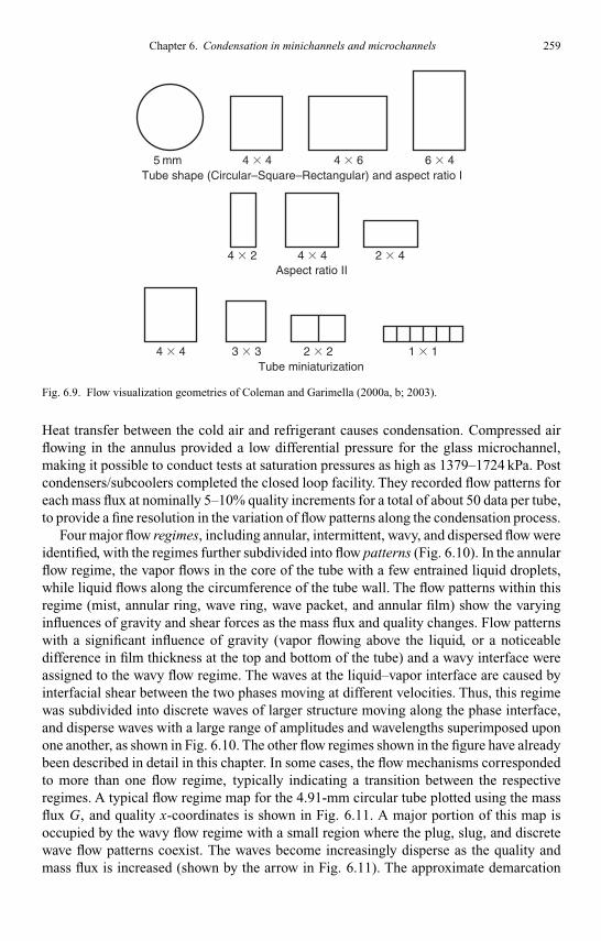
Kandlikar I044527-Ch06.tex 26/10/2005 18: 15 Page 259
Chapter 6. Condensation in minichannels and microchannels 259
5 mmTube shape (Circular–Square–Rectangular) and aspect ratio I
Aspect ratio II
Tube miniaturization
4 4
4 44 2 2 4
1 12 23 34 4
4 6 6 4
Fig. 6.9. Flow visualization geometries of Coleman and Garimella (2000a, b; 2003).
Heat transfer between the cold air and refrigerant causes condensation. Compressed airflowing in the annulus provided a low differential pressure for the glass microchannel,making it possible to conduct tests at saturation pressures as high as 1379–1724 kPa. Postcondensers/subcoolers completed the closed loop facility. They recorded flow patterns foreach mass flux at nominally 5–10% quality increments for a total of about 50 data per tube,to provide a fine resolution in the variation of flow patterns along the condensation process.
Four major flow regimes, including annular, intermittent, wavy, and dispersed flow wereidentified, with the regimes further subdivided into flow patterns (Fig. 6.10). In the annularflow regime, the vapor flows in the core of the tube with a few entrained liquid droplets,while liquid flows along the circumference of the tube wall. The flow patterns within thisregime (mist, annular ring, wave ring, wave packet, and annular film) show the varyinginfluences of gravity and shear forces as the mass flux and quality changes. Flow patternswith a significant influence of gravity (vapor flowing above the liquid, or a noticeabledifference in film thickness at the top and bottom of the tube) and a wavy interface wereassigned to the wavy flow regime. The waves at the liquid–vapor interface are caused byinterfacial shear between the two phases moving at different velocities. Thus, this regimewas subdivided into discrete waves of larger structure moving along the phase interface,and disperse waves with a large range of amplitudes and wavelengths superimposed uponone another, as shown in Fig. 6.10. The other flow regimes shown in the figure have alreadybeen described in detail in this chapter. In some cases, the flow mechanisms correspondedto more than one flow regime, typically indicating a transition between the respectiveregimes. A typical flow regime map for the 4.91-mm circular tube plotted using the massflux G, and quality x-coordinates is shown in Fig. 6.11. A major portion of this map isoccupied by the wavy flow regime with a small region where the plug, slug, and discretewave flow patterns coexist. The waves become increasingly disperse as the quality andmass flux is increased (shown by the arrow in Fig. 6.11). The approximate demarcation
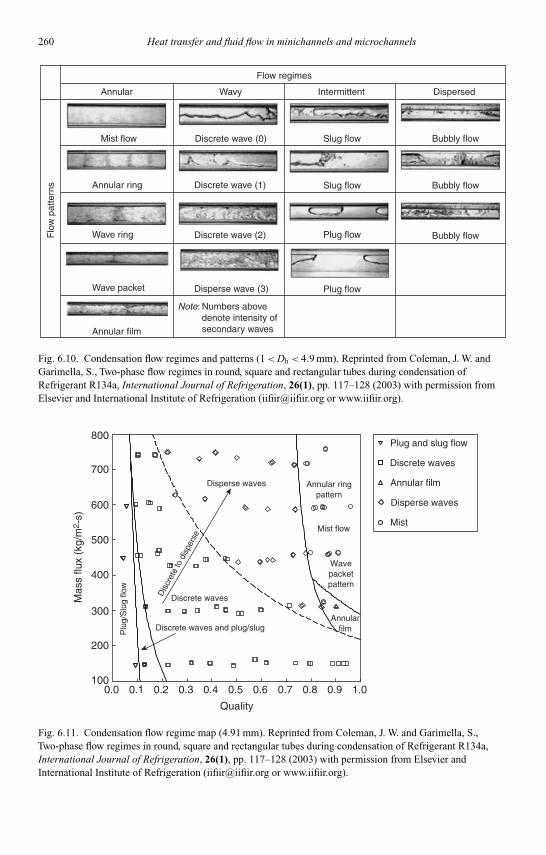
Kandlikar I044527-Ch06.tex 26/10/2005 18: 15 Page 260
260 Heat transfer and fluid flow in minichannels and microchannels
Flow regimes
Annular
Mist flow
Annular ring
Wave ringFlo
w p
atte
rns
Wave packet
Annular film
Numbers abovedenote intensity ofsecondary waves
Note:
Discrete wave (1)
Discrete wave (2)
Disperse wave (3)
Discrete wave (0) Slug flow
Slug flow
Plug flow
Plug flow
Bubbly flow
Bubbly flow
Bubbly flow
Wavy Intermittent Dispersed
Fig. 6.10. Condensation flow regimes and patterns (1<Dh < 4.9 mm). Reprinted from Coleman, J. W. andGarimella, S., Two-phase flow regimes in round, square and rectangular tubes during condensation ofRefrigerant R134a, International Journal of Refrigeration, 26(1), pp. 117–128 (2003) with permission fromElsevier and International Institute of Refrigeration ([email protected] or www.iifiir.org).
Quality
0.0 0.1 0.2 0.3 0.4 0.5 0.6 0.7 0.8 0.9 1.0
Mas
s flu
x (k
g/m
2 -s)
100
200
300
400
500
600
700
800
Mist flow
Disperse waves
Discrete waves
AnnularfilmP
lug/
Slu
g flo
w
Discrete waves and plug/slug
Mist
Annular film
Discrete waves
Disperse waves
Plug and slug flow
Annular ringpattern
Wavepacketpattern
Dis
cret
e to
dis
pers
e
Fig. 6.11. Condensation flow regime map (4.91 mm). Reprinted from Coleman, J. W. and Garimella, S.,Two-phase flow regimes in round, square and rectangular tubes during condensation of Refrigerant R134a,International Journal of Refrigeration, 26(1), pp. 117–128 (2003) with permission from Elsevier andInternational Institute of Refrigeration ([email protected] or www.iifiir.org).
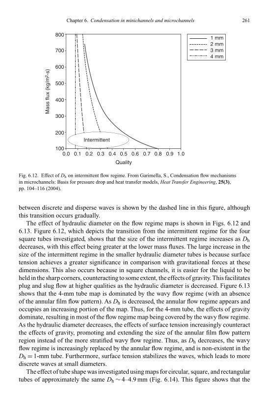
Kandlikar I044527-Ch06.tex 26/10/2005 18: 15 Page 261
Chapter 6. Condensation in minichannels and microchannels 261
800
700
600
500
400
300
200
1000.0 0.1 0.2 0.3 0.4 0.5
Quality
Mas
s flu
x (k
g/m
2 -s)
0.6 0.7 0.8 0.9 1.0
Intermittent
1 mm2 mm3 mm4 mm
Fig. 6.12. Effect of Dh on intermittent flow regime. From Garimella, S., Condensation flow mechanismsin microchannels: Basis for pressure drop and heat transfer models, Heat Transfer Engineering, 25(3),pp. 104–116 (2004).
between discrete and disperse waves is shown by the dashed line in this figure, althoughthis transition occurs gradually.
The effect of hydraulic diameter on the flow regime maps is shown in Figs. 6.12 and6.13. Figure 6.12, which depicts the transition from the intermittent regime for the foursquare tubes investigated, shows that the size of the intermittent regime increases as Dhdecreases, with this effect being greater at the lower mass fluxes. The large increase in thesize of the intermittent regime in the smaller hydraulic diameter tubes is because surfacetension achieves a greater significance in comparison with gravitational forces at thesedimensions. This also occurs because in square channels, it is easier for the liquid to beheld in the sharp corners, counteracting to some extent, the effects of gravity. This facilitatesplug and slug flow at higher qualities as the hydraulic diameter is decreased. Figure 6.13shows that the 4-mm tube map is dominated by the wavy flow regime (with an absenceof the annular film flow pattern). As Dh is decreased, the annular flow regime appears andoccupies an increasing portion of the map. Thus, for the 4-mm tube, the effects of gravitydominate, resulting in most of the flow regime map being covered by the wavy flow regime.As the hydraulic diameter decreases, the effects of surface tension increasingly counteractthe effects of gravity, promoting and extending the size of the annular film flow patternregion instead of the more stratified wavy flow regime. Thus, as Dh decreases, the wavyflow regime is increasingly replaced by the annular flow regime, and is non-existent in theDh = 1-mm tube. Furthermore, surface tension stabilizes the waves, which leads to morediscrete waves at small diameters.
The effect of tube shape was investigated using maps for circular, square, and rectangulartubes of approximately the same Dh ∼ 4–4.9 mm (Fig. 6.14). This figure shows that the

Kandlikar I044527-Ch06.tex 26/10/2005 18: 15 Page 262
262 Heat transfer and fluid flow in minichannels and microchannels
0.0
800
700
600
500
400
300
200
1000.1 0.2 0.3 0.4 0.5
Quality0.6 0.7 0.8 0.9 1.0
1 1 mm2 2 mm3 3 mm
Mas
s flu
x (k
g/m
2 -s) Annular
(1 mm)
Annular
(2 mm)
Annular
(3 mm)
Fig. 6.13. Effect of Dh on annular flow regime. From Garimella, S., Condensation flow mechanismsin microchannels: Basis for pressure drop and heat transfer models, Heat Transfer Engineering, 25(3),pp. 104–116 (2004).
Quality
0.0 0.1 0.2 0.3 0.4 0.5 0.6 0.7 0.8 0.9 1.0100
200
300
400
500
600
700
800
Annular
Wavy
Inte
rmitt
ent
Discrete wave
Disperse wave
Major transitions Discrete-to-disperse wave
Round (4.91 mm)Square (4 4 mm)Rectangular 4 (H) 6 (W) mmRectangular 6 (H) 4 (W) mm
Mas
s flu
x (k
g/m
2 -s)
Fig. 6.14. Effect of tube shape on flow regime transitions. From Garimella, S., Condensation flow mechanismsin microchannels: Basis for pressure drop and heat transfer models, Heat Transfer Engineering, 25(3),pp. 104–116 (2004).
Kandlikar I044527-Ch06.tex 26/10/2005 18: 15 Page 263
Chapter 6. Condensation in minichannels and microchannels 263
intermittent regime is larger in the round tube than in the square tube at lower mass fluxesand approximately the same at higher mass fluxes. The extent of the intermittent regimefor the rectangular tubes is in between that of the circular and square tubes. The wavyflow regime is also larger in the round tube. The square and rectangular channels helpliquid retention in the corners and along the entire circumference of the tube leading toannular flow, rather than preferentially at the bottom of the tube as would be the case inthe wavy flow regime. In the 4 × 6-mm and 6 × 4-mm tubes, the larger aspect ratio resultsin a slight increase in the size of the intermittent regime at the lower mass fluxes, and asmall reduction in the size of this regime at the higher mass fluxes. However, these effectsare small, and it can be concluded that this transition line is only weakly dependent onthe aspect ratio. The smaller aspect ratio also results in a larger annular film flow patternregion, which is to be expected because of the reduced influence of gravity for the tubeswith the smaller height. Discrete waves are more prevalent in the round tube comparedto the square and rectangular tubes. It was also found that the smaller aspect ratio resultsin a smaller wavy flow regime but with a larger fraction of discrete waves. At the highermass fluxes, the effect of the aspect ratio is negligible. The increase in the annular filmflow pattern region was more pronounced in the smaller hydraulic diameter tubes tested bythem, perhaps due to the greater influence of surface tension. Thus, while tube shape hadsome effect on the transitions between the various flow regimes, the influence of hydraulicdiameter was found to be far more significant.
A two-part study on flow regimes and heat transfer during condensing flows in channelswith 3.14<D< 21 mm has also appeared recently (El Hajal et al., 2003; Thome et al.,2003). Although this work is primarily on large channels, the comprehensive nature of thedatabase used for model development warrants discussion in this chapter. However, due tothe highly coupled nature of the flow regime (El Hajal et al., 2003) and heat transfer parts(Thome et al., 2003), it is presented in a subsequent section on heat transfer.
6.2.3. Summary observations and recommendations
The above discussion has shown that numerous studies have been conducted to understandtwo-phase flow in small diameter channels. The preponderance of studies is on adiabaticair–water flows. While these flows have historically provided some understanding of con-densation phenomena, many of the discrepancies between the behavior observed in thesestudies and the actual flow regimes during the condensation process can be attributed to thesubstantially different properties of the air–water pair compared to refrigerant vapor/liquidpair. It also appears that video recording technology is affording investigators the abilityto capture every nuance of two-phase flow in great detail. High-speed video presents theinvestigator with a plethora of images separated in time by very small increments. Whilethis is certainly advantageous in understanding the intricacies of two-phase flow, it has ledto the further proliferation of creative, confusing, and vague definitions of flow patterns.Just the number of flow patterns cited in this chapter alone would approach about 50!There are many definitions with relatively less distinction. Flow patterns from differentinvestigators can be as easily thought to agree as not, depending on the interpretation ofthese terms. As one who has himself pored over numerous frames of high-speed video, itis easy to understand how each researcher attempts to capture every nuance of a dynamic

Kandlikar I044527-Ch06.tex 26/10/2005 18: 15 Page 264
264 Heat transfer and fluid flow in minichannels and microchannels
bubble or a wave in a description of the pattern. It is not clear whether such detaileddescriptions have led to a significant advancement in the quantification of the relevantphysical phenomena that are responsible for these mechanisms in the first place. Theseminute distinctions between flow patterns would only be useful if they lead to quantitativemodels of essential features such as interfacial area, shear, slip, void fraction, momentumcoupling, and ultimately, heat transfer and pressure drop.
The summary evaluation of the above-mentioned studies is as follows:
(1) Adiabatic flow patterns are now available for a wide range of microchannels, mostlyusing air or nitrogen/water mixtures, all the way down to 25 µm. Extrapolation ofair–water flow patterns to condensing refrigerant applications must be done withcaution, however.
(2) Many of the studies on small circular and narrow rectangular channels were con-ducted on co- or countercurrent vertical upflow, which is an orientation seldom usedin condensation.
(3) It has now been very well documented that gravitational forces have little significancein the small channels (D<∼1 mm) of interest in this book. This has been validatedthrough observations of symmetric films, bubbles and slugs, and also flow patternsindependent of channel orientation.
(4) In the channels with 1<D< 10 mm, the flow patterns can broadly be classifiedas disperse, annular, wavy, and intermittent. Most of the phase-change studies inthis size range have focused on channels with D> 3 mm, and the primary focusof most of these investigations has been to understand gravity-dominated versusshear-controlled condensation.
(5) In channels with D< 1 mm, it appears that the primary patterns are some kind ofslug/plug flow, a transition region designated as liquid ring by some investigators,and annular flow (with some mist flow at high qualities and mass fluxes).
(6) Maps and transition criteria such as those by Taitel–Dukler (1976) are tempting touse because of their analytical basis; however, rarely do they predict condensationphenomena in microchannels – the original investigators perhaps never intended forthem to be applied in this manner.
(7) For the ∼5-mm channels, simple criteria such as those by Breber et al. (1980),Tandon et al. (1982), and Soliman (1982; 1986) may suffice, with minor modifi-cations to match the application under consideration to distinguish between gravityand shear-controlled condensation. The more recent descriptive reporting of flowpatterns by Dobson and Chato (1998) may also be used to obtain qualitative insights.
(8) While flow pattern descriptions are available for channels with D<∼5 mm, and evenfor channels in the 50–250 µm range, explicit equations that quantify the transitioncriteria are still missing. A combination of the analytical approaches ofTabatabai andFaghri (2001), some of the analyses of Mishima and Ishii (1996), and the ongoingwork of Kawahara, Kawaji, and others (Kawahara et al., 2002; Chung and Kawaji,2004) can be brought to bear to obtain such criteria.
(9) In addition, transition criteria that are applicable over a wide range of fluid properties,operating conditions, and channel sizes must be developed based on the underlyingforces and validated by the detailed experimentally obtained phase-change mapssuch as those of Coleman and Garimella (2000a, b; 2003) and Garimella (2004).

Kandlikar I044527-Ch06.tex 26/10/2005 18: 15 Page 265
(10) Similarly, the investigators of microchannels with D<< 1 mm should also test con-densation processes to supplement the information gathered from adiabatic flowvisualization studies.
The assignment of flow regimes for nine representative cases (combinations of massfluxes and qualities) for condensation of refrigerant R-134a in a 1-mm diameter channelusing several of the prominent transition criteria is illustrated in Example 6.1.
6.3. Void fraction
6.3.1. Conventional tubes
An important parameter for the calculation of heat transfer coefficients, and more sopressure drops, is the void fraction in two-phase flow. The void fraction also determinesthe amount of fluid to be charged into a closed loop system such as a refrigeration cycle.Void fraction is simply the ratio of the cross-sectional area Ag occupied by the gas, to thetotal cross-sectional area of the channel (see Table 6.2):
α = Ag
A(6.19)
The calculation of this parameter is an essential step and provides closure to the set ofequations that must be solved to estimate the pressure drop and heat transfer in two-phaseflow. While the vapor quality x is a thermodynamic quantity determined by the state ofthe two-phase mixture, the void fraction depends on the characteristics of the flow, andhas been the subject of several investigations. The slip, that is, the ratio of the velocitiesof the two phases, is required to enable computation of the void fraction. The simplestassumption that can be made is of homogeneous flow, where it is assumed that the vapor-and liquid-phase velocities are equal, and that the two phases behave like a single, uniformmixture that has representative average properties, which yields the following expression:
α = xρv
(1 − x)/ρl + x/ρv(6.20)
While the homogeneous model is in fact quite arbitrary, and serves as a starting point for themore representative models of void fraction, it has gained some acceptance for the modelingof microchannels, as will be discussed later. Void fraction models for conventional channelsare readily available in textbooks such as those by Carey (1992), Collier andThome (1994),and Hewitt et al. (1994); therefore, the more prominent correlations are simply presentedhere without discussion. While the details of the flow patterns must be taken into account toobtain models based on the physical phenomena, several of the more widely used correla-tions often assume annular flow and relate the void fraction to a parameter that resemblesthe Martinelli parameter X , often Xtt (which assumes turbulent flow in both phases).Incorporating the appropriate expressions for the pressure drops in the two phases, theseexpressions can be represented by the following generic expression (Butterworth, 1975):
α =[
1 + BB
(1 − x
x
)n1(ρv
ρl
)n2(µl
µv
)n3]−1
(6.21)

Kandlikar
I044527-Ch06.tex
26/10/200518:15
Page266
266H
eattransferand
fluidflow
inm
inichannelsand
microchannels
Table 6.2Summary of void fraction studies.
Hydraulic Range/Investigator diameter Fluids Orientation applicability Techniques, basis, observations
Conventional tubesPremoli et al. (1971) • Slip ratio-based correlation
Smith (1969) 6 mm Boiling Vertical 0.7< p< 5.9 MPa • Semi-empirical modelheavy 0< x< 0.38 • Assumed stratified annular flow (liquid-phase) with liquidwater 650<G< 2050 kg/m2-s entrainment in vapor-phase (homogeneous mixture phase),
380< q′′ < 1200 kW/m2 equal velocity head in both phases38 mm Boiling Horizontal, 1.725< p< 14.5 MPa • States that is model independent of flow regime, p, G, x; applicable
water vertical 0.003< x< 0.17 to horizontal and vertical co-current flow750<G< 1950 kg/m2-s • For K = 0.4, applicability assumed only for circular tubes20< q′′ < 140 kW/m2 • Not recommended for x< 0.01 in boiling flow (due to thermal
11 mm Air–water Vertical Atmospheric pressure inequilibrium)0.005< x< 0.52550<G< 1330 kg/m2-s
Zivi (1964) Several Steam–water Horizontal, • Analytical void fraction model (assuming annular flow),vertical minimizes rate of energy dissipation
• Three models: (I) without liquid entrainment and wall friction,(II) with wall friction, and (III) with liquid entrainment
• Data show wall friction effect << effect of liquid entrainment• As p increases, model (I) approaches homogeneous model• Simplest model (I) widely used, does not rely on data
Tandon et al. 6.1 mm Boiling Vertical 0.7< p< 6 MPa, • Semi-empirical void fraction model(1985b) heavy water x< 0.41 • Assumed annular flow without liquid entrainment in vapor-phase
650<G< 2050 kg/m2-s and turbulent flow in both phases380< q′′ < 1200 kW/m2 • State that model performs as well as Smith’s model (1969)0.24<α< 0.92 and better than Wallis’ (1969) and Zivi’s (1964) correlations
22 mm Steam–water Atmospheric pressurex< 0.04

Kandlikar
I044527-Ch06.tex
26/10/200518:15
Page267
Yashar et al. • Microfin tubes: R-134a, Horizontal 75<G< 700 kg/m2-s • Measurements in condensing microfin tubes (uncertainty 10%)(2001) 0.2-mm fin height R-410A 0.05< x< 0.8 • Similar trends for microfin and smooth tubes
• 7.3, 8.9 mm • Lower void fractions compared to evaporation, for same G, x(evaporation) • No effect of fin arrangement (helix angle)
• 8.9 mm(condensation)
El Hajal et al. 8 mm R-22, Horizontal 65<G< 750 kg/m2-s • Used earlier boiling maps (Kattan et al., 1998a, b, c;(2003) R-134a, (condensing) 0.22< pS < 3.15 MPa Zurcher et al., 1999) as basis
R-236ea, 0.15< x< 0.88 • Deduced void fractions for annular flow from heat transferR-125, database (Cavallini et al., 2001; 2002a, b)R-32, and film thickness considerationsR-410A • Logarithmic mean of homogeneous and Steiner (1993) models
Koyama et al. 7.52 mm R-134a Horizontal 0.01< x< 0.96 • Void fraction increases as pressure decreases (smooth and microfin)(2004) (smooth) (adiabatic) p = 0.8, 1.2 MPa • Smooth-tube data agree with Smith’s (1969) and Baroczy’s
8.86 mm G = 125, 250 kg/m2-s (1965) models(microfin) (smooth) • Microfin tube data lower than smooth tube values
G = 90, 180 kg/m2-s • Results different from Yashar et al. (2001), who reported similar(microfin) values for both tube types
• Yashar et al. (2001) correlation overpredicts microfin tube data• α in microfin tubes increases with increasing G, at low p, x• Model for stratified–annular and annular flow; reasonable
agreement with data, especially at high x
Small channelsArmand (1946) Air–water Horizontal β< 0.9 • Empirical correlation
atmospheric pressure
Kariyasaki 1, 2.4, Air–water Horizontal 0.1< jG < 25 m/s • Numerous curve-fits to match data without physical considerationset al. (1991) 4.9 mm 0.03< jL < 2 m/s
Mishima and 1–4 mm Air–water Vertical 0.0896< jG < 79.3 m/s • Image processing from neutron radiography forHibiki (1996) 0.0116< jL < 1.67 m/s non-intrusively measuring void fraction
• Correlated void fraction using drift-flux model with empiricalparameters for vertical bubbly and slug flow
(Continued )

Kandlikar
I044527-Ch06.tex
26/10/200518:15
Page268
Table 6.2(Continued)
Hydraulic Range/Investigator diameter Fluids Orientation applicability Techniques, basis, observations
• Distribution parameter function of D, larger valuesfor small channels than reported by Ishii (1977) for larger tubes
• Agreed with Kariyasaki et al. (1992) correlation
Hibiki and 1–4 mm Air–water Vertical j< 19 m/s • Best agreement with 1-mm dataMishima (1996) • Technique also works for annular flow at high α in larger tubes
Hibiki et al. (1997) 3.9 mm Air–water Vertical jG = 0.131 m/s • Correlation for radial void fraction profile for vertical slug flowupward jL = 0.0707 m/s
Mishima 2.4 mm Air–water Vertical j< 8 m/s • Neutron radiography image processing for variation ofet al. (1997) upward void fraction along channel length for slug flow
• Rise of bubble tracked using high void fraction region• Merging of void fraction peaks indicated bubble coalescence
Kureta et al. 3, 5 mm Steam–water Vertical 240 < G < 2000 kg/m2-s • Instantaneous and time-averaged 2-D α for subcooled(2001; 2003) upward boiling (at low α)
Triplett et al. 1.1, 1.45 mm Air–water Horizontal 0.02< jG < 80 m/s • Volumetric void fraction from still photographs (rotational(1999a) (adiabatic) 0.02< jL < 8 m/s symmetry assumed, uncertainty ∼15%)
• Void fraction increases with increasing gas velocity anddecreases with increasing superficial liquid velocity
• Homogeneous model best for slug and bubble flow,Premoli et al. (1971), Chexal et al. (Chexal and Lellouche, 1986;Chexal et al., 1992; Chexal et al., 1997), Lockhart–Martinelli(1949), Baroczy (1965) overpredict for annular and churn flow
MicrogravityElkow and 9.525 mm Air–water Vertical 0.1< jG < 18 m/s • PDF of void fluctuations at 1-g, µ-g with capacitance sensorRezkallah upward 0.07< jL < 2.5 m/s • Average α in slug flow ∼10% higher at µ-g(1997a, b) (adiabatic) 0.1<α< 0.9 • Larger α fluctuations in bubble and slug flow at 1-g
• Fluctuations decreased in transitional and annular flow,due to increasing dominance of inertia forces
• Compared with drift-flux model, at 1-g: power law distributionin slug flow, saddle-shaped distribution in bubbly flow;at µ-g, power law distribution for both flows

Kandlikar
I044527-Ch06.tex
26/10/200518:15
Page269
Lowe and 9.525 mm Air–water Vertical 0.09< jG < 20.94 m/s • Capacitance sensor to measure α, identify flow regimes usingRezkallah upward 0.04< jL < 3.03 m/s time trace and PDF(1999) p = 89 kPa, µ-g, 1-g
MicrochannelsSerizawa 20, 25, 100, Air–water Horizontal 0.0012< jG < 295.3 m/s • α in bubbly and slug flow from video analysiset al. (2002) 50 µm (steam–water) 0.003< jL < 17.52 m/s • Follows Armand (1946) and Kariyasaki et al. (1991) correlations
Kawahara 100 µm Nitrogen–water Horizontal 0.1< jG < 60 m/s • Time-averaged void fraction and curve-fit from video analysiset al. (2002) 0.02< jL < 4 m/s • α increases with increasing homogenous void fraction. Very low α
for β< 0.8, rapid increase for β> 0.8• Different from Serizawa et al. (2002) who found linear
correlation to homogeneous α for similar diameters• Low α at high gas flow rates indicates large slip ratios
and weak momentum coupling between phases
Chung and 50, 100, 250, Nitrogen–water Horizontal T = 22.9–29.9◦C • 530 µm: homogeneous model, 250 µm: Armand (1946) correlation,Kawaji (2004) 530 µm 0.02< jG < 72.98 m/s 50, 100 µm: Kawahara et al. (2002) correlation
0.01< jL < 5.77 m/s • Slightly different constants for 50-µm channel
Chung 96-µm square Nitrogen–water Horizontal 0.000310< Bo< • Kawahara et al. (2002) correlation holds for 96 µm square channelet al. (2004) (adiabatic) 0.000313
0.00010<WeLS < 250.000019<WeGS < 91<ReLS < 4381<ReGS < 612
Kawahara 50, 75, Water–Nitrogen, Horizontal 0.08< jG < 70 m/s • No effects of fluid propertieset al. (2005) 100, 251 µm Ethanol–water/ 0.02< jL < 4.4 m/s • 50-, 75-, 100 µm data follow Kawahara et al. (2002) correlation,
nitrogen 251 µm data follow linear Armand (1946) correlation• Used to demarcate micro-/minichannels (100–251 µm)

Kandlikar I044527-Ch06.tex 26/10/2005 18: 15 Page 270
270 Heat transfer and fluid flow in minichannels and microchannels
A convenient tabulation of the leading coefficient BB and the exponents n1 . . . n3 forthis model appears in Carey (1992) for the Zivi (1964) entropy minimization model, theWallis (1969) separated cylinder model, the Lockhart–Martinelli (1949) model, the Thom(1964) correlation, and the Baroczy (1965) correlation. Hewitt et al. (1994) also providethe following correlation developed by Premoli et al. (1971) based on the slip ratio uG/uL:
S = 1 + E1
[(y
1 + yE2
)− yE2
]1/2
(6.22)
where y =β/1 − β, and β is the volume ratio (also equivalent to the homogeneous voidfraction):
β = xρL
xρL + (1 − x) ρG(6.23)
The parameters E1 and E2 are given by:
E1 = 1.578Re−0.19LO
(ρL
ρG
)0.22
E2 = 0.0273WeLORe−0.51LO
(ρL
ρG
)−0.08 (6.24)
where ReLO = GD/µL and WeLO = G2D/σρL. Once the slip ratio is calculated using theabove equations, the void fraction is obtained as follows:
α = x
x + S (1 − x) ρG/ρL(6.25)
Several investigators have also used the void fraction by Smith (1969), which was basedon an annular flow assumption, and also assumed equal velocity heads of the core andannular film flows. Smith stated that this correlation, given below, can be used irrespectiveof flow regime, pressure, mass flux, quality, and other parameters:
α =
1 +
(ρG
ρL
)(1 − x
x
)×0.4 + 0.6
√√√√(ρLρG
)+ 0.4
( 1−xx
)1 + 0.4
( 1−xx
)
−1
(6.26)
Tandon et al. (1985b) developed an analytical model for the void fraction in annular flows.They assumed an axi-symmetric annular film and a core with no liquid entrainment, andturbulent flow in both phases, which was justified based on Carpenter and Colburn’s (1951)finding that at high gas velocities, the liquid phase laminar–turbulent transition could occurat ReL ∼ 240. Frictional pressure drops were computed using the Lockhart–Martinelli(1949) method, and the von Karman universal velocity profile was used to represent thevelocity distribution in the liquid film. They found good agreement with data from Isbinet al. (1957) for steam–water flow through a 22-mm tube, and Rouhani and Becker (1963)for boiling of steam in 6.1-mm vertical tubes, and also with the correlation of Smith et al.

Kandlikar I044527-Ch06.tex 26/10/2005 18: 15 Page 271
Chapter 6. Condensation in minichannels and microchannels 271
(1969). The void fraction is related to the liquid film Reynolds number and the Martinelliparameter as follows:
α ={
1 − 1.928Re−0.315L [F (Xtt)]−1 + 0.9293Re−0.63
L [F (Xtt)]−2}
50 < ReL < 1125
α ={
1 − 0.38Re−0.088L [F (Xtt)]−1 + 0.0361Re−0.176
L [F (Xtt)]−2}
ReL > 1125
(6.27)
where F(Xtt) = 0.15[X −1tt + 2.85X −0.476
tt ].A review of the applicability of several different void fraction models appears in Rice
(1987), who pointed out that the choice of the void fraction model affects refrigerant chargeprediction to a significant degree, and that models based on non-refrigerant fluids, geome-tries, and flow conditions yield high levels of uncertainty when applied to refrigerants.Improper charge prediction can lead to problems in off-design and transient performance.
Yashar et al. (2001) pointed out that commonly used void fraction models (Smith, 1969;Wallis, 1969; Premoli et al., 1971) are best suited for evaporation applications due to theirbasis in air–water flows or in water boiling applications. As stated previously in this chapter,air–water and steam–water mixtures are characterized by low gas-phase densities, whereasin condensation, particularly of refrigerants, the vapor-phase density is much higher dueto the higher pressures involved. Due to these higher vapor-phase densities, the vaporvelocities are lower, which favors stratified flows, and leads to a dependence of the voidfraction on mass flux – a feature that is often not included in several of the widely usedmodels. Noting that transitions between stratified and annular regions are in fact gradualdue to the movement of the liquid film up around the circumference of the tube withincreasing velocities, Hurlburt and Newell (1999) developed a model for the non-uniformfilm thickness during this stratified–annular transition. (It was pointed out in the previoussection that other investigators have refereed to this region as semi-annular or wavy flow.)Graham et al. (1999) attempted to account for the dependence of the void fraction on thenon-uniform film thickness by using the Froude rate (Yashar et al. 2001), a parameter thatcompares the vapor kinetic energy to the energy required to move the liquid phase upwardalong the circumference. Thus, the Froude rate parameter is the Froude number multipliedby the square root of the vapor-to-liquid mass flow rate ratio:
Ft =[
G2x3
(1 − x) ρ2ggD
]0.5
(6.28)
They reasoned that variation of the void fraction during the transition from stratified toannular flow would be accounted for by this parameter (vapor kinetic energy/gravitationaldrag) combined with the Lockhart–Martinelli parameter (viscous drag/vapor kineticenergy), and proposed the following expression:
α =[
1 + 1
Ft+ Xtt
]−0.321
(6.29)
In the above expression, both phenomena are assumed to act independently. Yashar et al.(2001) measured void fractions during condensation in microfin (0.2-mm fin height) tubes

Kandlikar I044527-Ch06.tex 26/10/2005 18: 15 Page 272
272 Heat transfer and fluid flow in minichannels and microchannels
of 8.9-mm diameter. Essentially, linked shutoff valves were actuated during tests to isolatethe inventory of the two-phase mixture in the test section, which provided the volume-averaged void fraction for the given test condition. (It should be noted that this technique,used by many investigators, does not provide the area fraction at a cross-section of thetube, which is the more relevant parameter, but rather a volumetric average.) These testsshowed that the trends for smooth and microfin tubes were similar and that for evaporation,the void fraction was relatively insensitive to mass flux. However, mass flux effects wereseen in condensation, particularly at low mass fluxes (G< 200 kg/m2-s), presumably dueto the larger vapor densities at condensing conditions.
Koyama et al. (2004) investigated void fractions for the adiabatic flow of R-134a in hori-zontal 7.52-mm smooth and 8.86-mm microfin tubes over the quality range 0.01< x< 0.96using quick closing valves, an approach similar to that used by Yashar et al. (2001). Thevoid fractions in the smooth tube agreed well with the Smith (1969) and Baroczy (1965)correlations. The void fractions were lower at the higher pressures, whereas the effectof mass flux was minimal. They also found that the void fractions in the microfin tubewere lower than those in the smooth tube; thus the smooth-tube void fraction models wereunable to predict the experimental values for the microfin tube. They stated that becauseof the higher pressure drop in the microfin tubes, the mean liquid velocity is lower and theliquid occupies a larger portion of the cross-section, which leads to lower void fractionsin the microfin tubes. The void fraction in microfin tubes was found to increase with anincrease in mass flux, particularly at low pressures and qualities. They also developedmodels for the void fraction in microfin tubes for stratified–annular and annular flow. Theyassumed that the liquid flows at the bottom of the tube and also fills the grooves aroundthe whole circumference in stratified–annular flow. For annular flow, they assumed thatthe grooves were filled uniformly. Using these assumptions, they iteratively solved simplemomentum balance equations between the vapor and liquid regions to obtain the voidfraction for the experimental conditions. They found reasonably good agreement betweenthe experimental and numerically predicted values, especially at high vapor qualities.
6.3.2. Small channels
For the small diameter range, Kariyasaki et al. (1991) measured void fraction in 1-, 2.4-,and 4.9-mm tubes and proposed several empirical curve-fits to the measured void fractionsin small regions as a function of the homogeneous volume fraction (see Table 6.2):
β < βA: α = β
βB < β < 0.6 (intermittent flow): α = 0.833ββB < β, 0.6 < β < 0.95 (intermittent flow): α = 0.69β + 0.0858βB < β, 0.95 < β (annular and intermittent flow): α = 0.83 log (1 − β)+ 0.633
(6.30)
where βA and βB are also empirically derived transition points. While the above correlationmatched their data, it appears to have been derived simply based on statistical curve-fits tofollow the data closely, and the trends exhibited show numerous unrealistic discontinuities,changes in slope and inflections for which no physical rationale is provided. The firstintermittent flow correlation above is the so-called Armand (1946) correlation.
Kandlikar I044527-Ch06.tex 26/10/2005 18: 15 Page 273
Chapter 6. Condensation in minichannels and microchannels 273
Mishima and Hibiki (1996) used neutron radiography to conduct flow visualizationstudies on air–water flows in 1–4-mm diameter tubes. The void fraction was correlatedwell by the drift-flux model with a new equation for the distribution parameter as a functionof inner diameter. The drift-flux model was used to correlate the void fraction as follows:
uG = jG/α = Co j + UG j (6.31)
where uG is the gas velocity, j is the mixture volumetric flux, j = jG + jL, Co is the dis-tribution parameter, and VGj is the drift velocity. For each regime (bubbly, slug, annularand churn), the required distribution parameter was taken from Ishii (1977). However, inaccordance with the findings of several other researchers (Gibson, 1913; Zukoski, 1966;Tung and Parlange, 1976; Kariyasaki et al., 1992), the drift velocity in slug and bubblyflows was assumed to be zero, and the distribution parameter was fit to the followingequation based on the data:
Co = 1.2 + 0.510e−0.691D (6.32)
where the tube diameter D is in mm. These findings were in good agreement with theresults of Kariyasaki et al. (1992), who modeled their data in terms of the volumetric voidfractionβ= jG/( jG + jL). The distribution parameters resulting from the data and the aboveequation for the small diameter channels are larger than those reported by Ishii (1977) forlarger channels. Mishima et al. (1993) also found this increase in Co for narrow rectangularchannels, and attributed this trend to the centralized void profile and the laminarizationof flow in these smaller and narrower channels. Hibiki and Mishima (1996) developedan approximate method for the processing of images obtained from neutron radiography,which was then used for non-intrusively measuring void fractions in air–water flows in tubeswith 1<D< 4 mm. The agreement between the data and the predictions of the radiographytechnique was best at 1 mm, but the technique was deemed to be acceptable for annularflows with large void fractions in the larger tubes also. Hibiki et al. (1997) then usedthe neutron radiography method to measure radial void fraction distributions in verticalupward air–water flow in a 3.9-mm channel. An assumed power law or saddle-shapedvoid fraction profile was subsequently verified using measured integrated variations in thevoid fraction profile along the channel axis. A triple-concentric-tube apparatus with somechannels filled with water or gas in different combinations provided baseline attenuationsand ensured calibration of the experimental results. The method was demonstrated bydeveloping the following equation for void fraction in slug flow:
αr = 0.8372 +[
1 −(
r
rw
)7.316]
(6.33)
The variation in void fraction along channel length in slug flow was determined by Mishimaet al. (1997), who used the images shown in the previous section on flow patterns (Fig6.2) to compute the void profile across the channel at intervals of 6.45 mm (Fig. 6.15).This figure shows that the high void fraction region moves upward with the rise of the slugbubble. Also, the merging of two peaks into one peak is illustrated, corresponding to thecoalescence of two bubbles. Unesaki et al. (1998) later conducted Monte Carlo simulationsfor the triple-concentric-tube apparatus described above to further validate the technique.

Kandlikar I044527-Ch06.tex 26/10/2005 18: 15 Page 274
274 Heat transfer and fluid flow in minichannels and microchannels
Flow directionSlug flow
t � 80 ms
t � 64 ms
t � 48 ms
t � 32 ms
t � 16 ms
t � 0 ms604020
00 20 60
Longitudinal position (mm)Voi
d fr
actio
n (%
)
40 80 100 120
Fig. 6.15. Progression of void fraction profiles with time. Reprinted from Mishima, K., Hibiki, T. andNishihara, H., Visualization and measurement of two-phase flow by using neutron radiography, NuclearEngineering and Design, 175(1–2), pp. 25–35 (1997) with permission from Elsevier.
This group (Kureta et al., 2001; 2003) also measured instantaneous and time-averagedvoid fractions for subcooled boiling of water (at low void fractions) in narrow rect-angular channels (3- and 5-mm gap) using neutron radiography in the mass flux range240<G< 2000 kg/m2-s. Although their primary objective was to determine the point ofnet vapor generation and its effect on critical heat flux, their technique and results demon-strate the feasibility of non-intrusively obtaining temporally (0.89 ms) and spatially (2-D)resolved void fractions in two-phase flows in minichannels. A representative distributionof instantaneous void fractions obtained by them is shown in Fig. 6.16. Such temporalresolution is particularly helpful for flows more prevalent in minichannels (such as slugflows) with large temporal variations in void fraction. Fig. 6.17 shows void fraction pro-files computed by averaging instantaneous values over 2 s (2250 images). Such techniquescould also be applied to gain detailed insights into condensing flows.
Triplett et al. (1999a, b) used still photographs of flow patterns in 1.1- and 1.45-mmhorizontal circular channels (although, as noted in the previous section, flow patterns werealso recorded for semi-triangular channels) to obtain the volumetric void fraction. Bubblesin the bubbly flow pattern were assumed to be spheres or ellipsoids, while the bubbles inslug flow were assumed to consist of cylinders and spherical segments. Annular flow voidfractions were estimated by averaging cylindrical segments of the vapor core. The estimateduncertainties in these void fractions were relatively high, 15%. Also, they were unable toreliably measure void fractions in slug-annular and churn flow, and assigned a void fractionof 0.5 to the portion of churn flow in which the gas phase was dispersed. In general theyfound that the void fraction increases with increasing gas superficial velocity, UGS at aconstant liquid superficial velocity, ULS, and decreases with increasing ULS for constantUGS. They compared their results with the void fraction correlations of Butterworth (1975),Premoli et al. (1971), and the correlation of Chexal et al. (Chexal and Lellouche, 1986;Chexal et al., 1992; Chexal et al., 1997), which is based on the drift-flux model of Zuber

Kandlikar I044527-Ch06.tex 26/10/2005 18: 15 Page 275
Chapter 6. Condensation in minichannels and microchannels 275
Voidfraction
Vaporbubble
Voidfraction
1
0100
(�)
50
0 �15Transverse
position (mm)
Flow-directionaldistance (mm)
1
0.5
0
(a) 0 ms (b) 10.7 ms (c) 21.3 ms
30 mm
100
mm
150
Fig. 6.16. Instantaneous 2-D void fraction profiles in narrow rectangular channels. Reprinted from Kureta, M.,Hibiki, T., Mishima, K. and Akimoto, H., Study on point of net vapor generation by neutron radiography insub-cooled boiling flow along narrow rectangular channels with short heated length, International Journal ofHeat and Mass Transfer, 46(7), pp. 1171–1181 (2003) with permission from Elsevier.
Flow-directional distance, z (mm)
s � 5 mm, G � 600 kg/(m2s), T in � 90°C
Voi
d fr
actio
n, �
(�
)
Transverseposition,d (mm)
15
0
�15
100
1
0.5
0
50
0
0.7 MW/m2
0.9 MW/m2
Fig. 6.17. Time-averaged 2-D void fraction in narrow rectangular channels. Reprinted from Kureta, M.,Hibiki, T., Mishima, K. and Akimoto, H., Study on point of net vapor generation by neutron radiographyin sub-cooled boiling flow along narrow rectangular channels with short heated length, InternationalJournal of Heat and Mass Transfer, 46(7), pp. 1171–1181 (2003) with permission from Elsevier.
and Findley (1965). They found that the homogeneous flow model was the best predictorof the measured void fractions in bubbly and slug flow, that is, at low UGS values. Forannular and churn flow, however, the homogeneous model and other empirical modelssignificantly overpredicted the experimental values. They believe that this overpredictionby the empirical correlations, typically based on annular flow in large channels, is due tothe slip being greater in the larger channels than in microchannels.
Kandlikar I044527-Ch06.tex 26/10/2005 18: 15 Page 276
276 Heat transfer and fluid flow in minichannels and microchannels
6.3.3. Microgravity
As mentioned in the previous section on flow regimes, Rezkallah and co-workers haveconducted investigations on two-phase flow in microgravity environments that pertainsto flows in small diameter channels due to the decreased influence of gravity. Elkow andRezkallah (1997a, b) conducted detailed measurements of void fraction fluctuations inearth normal (vertical upward) and microgravity conditions for air–water flow in a 9.53-mmtube. Such fluctuations were also measured by Jones and Zuber (1975) using signalsfrom gamma densitometers, by Weisman et al. (1979) (discussed in the previous section)using pressure signals, by Das and Pattanayak (1993; 1994a, b; 1995a, b; 1996) andMatuszkiewicz et al. (1987) using impedance and conductivity probes, respectively, andby Geraets and Borst (1988) and Keska et al. (1992) using capacitance probes. Probabilitydensity functions (PDFs) of the void fraction fluctuations were larger in the bubble and slugflow regimes at 1-g compared to those at microgravity. This difference decreased as inertiaforces became more predominant in transitional and annular flows. They inferred that atmicrogravity conditions, the slip velocity in bubble flow is almost zero – an observationmade by several others cited in this chapter, and the bubble movement and liquid turbulenceare highly suppressed. In slug flow, the average void fraction values at 1-g were found tobe ∼10% lower than those at microgravity. The void fraction signal fluctuated from high tolow values, based on whether the channel was occupied by the liquid or the gas phase. At1-g, bubbles coalesce readily due to contact betweenTaylor bubbles, leading to fluctuationsin the void fraction (0–0.75), while at microgravity, Taylor bubbles did not interact witheach other, resulting in much smaller void fraction fluctuations (0.3–0.55). The relationshipbetween the volumetric void fraction β and the area-based void fraction α can be expressedas follows (see Table 6.2):
〈β〉〈α〉 = Co +
⟨αUG j
⟩〈α〉 〈 j〉 (6.34)
where UGj is the previously defined drift velocity and j is the volumetric flux,( j = USG + USL). The distribution coefficient Co = 〈αj〉/(〈α〉〈 j〉) accounts for the non-uniform distribution of the void fraction over the cross-section of the tube, and depends onthe flow regime and the void fraction profile. In microgravity flow, the second term above(drift velocity) was neglected (as was the case with other investigators discussed above),which yielded a distribution coefficient of 1.25 in bubbly and slug flow (centerline voidfraction > wall void fraction). The distribution coefficient being the same for bubbly andslug flows at zero gravity is because of the slip between the two phases being negligiblein both types of flow. While Co at 1-g in slug flow was close to this value (Co = 1.17), inbubbly flow, it was found to be 0.61, indicating a saddle-shaped void fraction profile, witha higher void fraction at the wall than at the center.
Lowe and Rezkallah (1999) developed this technique further, using a concave parallelplate capacitance sensor to measure void fractions for identifying flow regimes. They wereable to define objective criteria for flow regime identification based on the void fractionPDF in conjunction with high-speed video images. An illustration of the different signalsand PDFs for the three primary flow regimes of interest in microchannels is shown in

Kandlikar I044527-Ch06.tex 26/10/2005 18: 15 Page 277
Chapter 6. Condensation in minichannels and microchannels 277
0 0.2
1.0 0.10
<ε> � 0.067
<ε> � 0.605
ε
εε
ε
ε
ε
<ε> � 0.879
0.090.080.070.060.050.040.030.020.010.00
0.06
0.05
0.04
0.03
0.02
0.01
0
0.90.80.70.60.50.40.30.20.10.0
�0.1
1.00.90.80.70.60.50.40.30.20.10.0
�0.1
1.00.90.80.70.60.50.40.30.20.10.0
�0.1
0.4 0.6
Time (s)(a1)
(a2)
(a3)
(b1)
(b2)
(b3)
Pro
babi
lity
Pro
babi
lity
0.30
0.25
0.15
0.20
0.10
0.05
0.00
Pro
babi
lity
0.8 �0.1 0 0.1 0.2 0.3 0.4 0.5 0.6 0.7 0.8 0.9 1 1.1
�0.1 0 0.1 0.2 0.3 0.4 0.5 0.6 0.7 0.8 0.9 1 1.1
�0.1 0 0.1 0.2 0.3 0.4 0.5 0.6 0.7 0.8 0.9 1 1.1
1
0 0.2 0.4 0.6
Time (s)
0.8 1
0 0.2 0.4 0.6
Time (s)
0.8 1
Fig. 6.18. Void fraction signals and PDF. Reprinted from Lowe, D. C. and Rezkallah, K. S., Flow regimeidentification in microgravity two-phase flows using void fraction signals, International Journal of MultiphaseFlow, 25(3), pp. 433–457 (1999) with permission from Elsevier.
Fig. 6.18. A low average void fraction signal with small fluctuations corresponding tothe passage of the bubbles, and a PDF with a single narrow peak at the low end of thevoid fraction range characterizes bubbly flow. A void fraction signal with large fluctuationsbetween high and low values corresponding to the passage of gas bubbles and liquid slugscharacterizes slug flow. The corresponding PDF has two peaks. Annular flow exhibits arelatively constant void fraction of about 0.80–0.90, with the PDF showing a very narrowpeak. Small dips in the void fraction trace correspond to the passage of disturbance waves.Such traces and PDFs were also used to identify transitions between the respective regimes.Packing densities of spherical and elongated bubbles were used to interpret the locationsof the transitions from slug-annular flow.
6.3.4. Microchannels
Serizawa et al. (2002) studied air–water flow in microchannels (20, 25, and 100 µm)and steam–water flow in a 50-µm tube. Although a variety of flow regimes (discussed in

Kandlikar I044527-Ch06.tex 26/10/2005 18: 15 Page 278
278 Heat transfer and fluid flow in minichannels and microchannels
the previous section) were identified by them, cross-sectional-averaged void fractions werecalculated from high-speed video pictures only for the bubbly and slug flow regimes (liquidring flow was not included for void fraction analysis). The Armand (1946) correlationα= 0.833β, discussed above in connection with the work of Kariyasaki et al. (1991), wasrecommended for these regimes (Table 6.2).
Kawahara et al. (2002) measured void fractions for nitrogen–water flow in a 100-µmtube by analyzing video frames and assigning a void fraction of 0 to the liquid slug, anda void fraction of 1 to a frame with a gas core surrounded by a smooth-thin liquid filmor ring-shaped liquid film. Time-averaged void fractions were then calculated over severalframes. For high liquid flow rates, gas-core flow with a thick liquid film was assigned a voidfraction (0<α< 1), thus accounting for a finite film thickness surrounding the core in suchflows. They found that the void fraction is not strongly dependent on jL, and developed thefollowing empirical fit for the void fraction in terms of the homogeneous void fraction:
α = 0.03β0.5
1 − 0.97β0.5 (6.35)
This variation of void fraction (Fig. 6.19) is significantly different from the linear rela-tionship with the homogeneous void fraction described above. Thus, void fractions remain
1.0
0.8
0.6
0.4
0.2
0.00.0 0.2
Homogeneous void fraction (b)
Voi
d fr
actio
n (�
)
0.4 0.6 0.8 1.0
Empirical correlation, Eq. (6.35)� � b, Homogeneous flow� � 0.8b, Ali et al. (1993)jL � 0.02–0.06 m/sjL � 0.11–0.20 ms/sjL � 0.42–0.56 m/sjL � 1.34–1.51 ms/sjL � 3.50–4.40 m/s
Fig. 6.19. Void fractions for air–water flow in 100-µm channels. Reprinted from Kawahara, A., Chung, P. M. -Y.and Kawaji, M. Investigation of two-phase flow pattern, void fraction and pressure drop in a microchannel,International Journal of Multiphase Flow, 28(9), pp. 1411–1435 (2002) with permission from Elsevier.

Kandlikar I044527-Ch06.tex 26/10/2005 18: 15 Page 279
Chapter 6. Condensation in minichannels and microchannels 279
low even at high values of β (β< 0.8), and increase steeply for 0.8<β< 1. They attributedthis phenomenon to the observation that single-phase liquid flow occurred most frequentlyat high liquid flow rates for all gas flow rates, and also at low liquid and gas flow rates.Wall shear and surface tension resulted in channel bridging under such conditions, andthe associated low average void fractions. At low liquid and high gas flow rates, gas-coreflow surrounded by a liquid film with weak momentum coupling was seen. While theliquid flow was governed by wall shear and surface tension, the gas phase flowed withoutsignificant resistance due to the undeformed shape characteristic of the flow in such smallchannels observed by them. The nonlinear dependence of the area-based void fraction onthe volumetric void fraction implies that slip ratios are much higher (as high as 16) in thesechannels compared to the much lower values seen in channels with Dh > 1 mm. It shouldbe noted that these results contradict the results of Serizawa et al. (2002), who reportedthe adequacy of the Armand correlation for a similar range of Dh.
Chung and Kawaji (2004) investigated the effect of channel diameter on void fractionfor the flow of nitrogen–water mixtures in circular 530-, 250-, 100-, and 50-µm channels.For the larger channels (530 and 250 µm), multiple images at each data point were ana-lyzed by estimating the gas fraction volume as a combination of symmetrical shapes. Forthe smaller channels, the void fraction was estimated as described above in Kawahara et al.(2002). They found that the void fraction for the 530-µm channel was predicted well bythe homogeneous flow model, and the void fraction for the 250-µm channel agreed wellwith the Armand-type correlation. However, the 100- and 50-µm channel void fractionsfollowed the slow linear increase up to β= 0.8, followed by a steep exponential increasecaptured by Eq. (6.35) above that was developed by them earlier (Kawahara et al., 2002).(Based on this latter work, however, they modified the leading constants for the 50-µmchannel to 0.02 and 0.98 in the numerator and denominator, respectively.) They attributedthe departure from homogeneous flow at high volumetric void fractions to a larger slipbetween the phases. This modified equation indicates a further decrease from the homo-geneous model, even compared to the values for the 100-µm channel. They argued thatin the larger (mini) channels, the wavy and deformed gas–liquid interface leads to moremomentum exchange between the gas and liquid phases, which slows the flow of the gasbubbles, keeping the void fraction high. On the other hand, according to them, the lackof this momentum exchange in the microchannels leads to a lower void fraction. Chunget al. (2004) later confirmed that the coefficients in the void fraction correlation for cir-cular 100-µm channels (C1 = 0.03, and C2 = 0.97) would apply to square channels withDh = 96 µm.
Kawahara et al. (2005) further investigated the effect of fluid properties and diameter onvoid fraction. They tested the two-phase flow of water–nitrogen and ethanol–water/nitrogengas mixtures (of varying ethanol concentrations) in 50-, 75-, 100-, and 251-µm circularchannels. Their results showed that the void fraction was not sensitive to fluid proper-ties over the range of diameters studied. The void fraction data for the 50-, 75-, and100-µm channels agreed with the correlation of Kawahara et al. (2002), but the datafor the 251-µm diameter channel followed the homogeneous flow type model of Armand(1946). They interpreted these results to imply that the boundary between “microchannels”and “minichannels” would lie between 100 and 251 µm.

Kandlikar I044527-Ch06.tex 26/10/2005 18: 15 Page 280
280 Heat transfer and fluid flow in minichannels and microchannels
6.3.5. Summary observations and recommendations
The above discussion has shown that void fraction models for conventional tubes have beendeveloped on the basis of an assumption of homogeneous flow, or as a function of slip ratio,the Lockhart–Martinelli parameter, and those that incorporate some dependence on themass flux. Many of these models assume annular flow regardless of the flow conditions.Also, several of these models were developed using data from air–water adiabatic flow,or evaporating flows, although in practice, they are routinely used for condensation also.Yashar et al. (2001) acknowledged the higher vapor phase densities in condensing flowscompared to air–water or evaporating flows, and pointed out that this leads to lower vaporvelocities, more stratified flows, and a dependence of the void fraction on mass flux. Thisgroup (Graham et al., 1999) also used a Froude Rate parameter and developed a simplemodel for the changing void fraction from stratified to annular flows by accounting for theratio of the vapor kinetic energy to the gravitational drag, combined with the Lockhart–Martinelli parameter, which accounts for the ratio of the viscous drag to the vapor kineticenergy. Linked shutoff valves were used by this group as well as by Koyama et al. (2004)to measure the vapor trapped in the test section, which yields the volumetric void fraction,but not the cross-sectional void fraction.
Mishima, Hibiki, and co-workers (Mishima et al., 1993; Hibiki and Mishima, 1996;Mishima and Hibiki, 1996; Hibiki et al., 1997; Mishima et al., 1997; Kureta et al.,2001; Kureta et al., 2003) have used neutron radiography to measure the distribution ofvoid fractions in 2-D in small channels, as well as the temporal evolution of the voidfraction, for example, as the vapor and liquid phases in slug flow pass through the regionof interest. Triplett et al. (1999a, b) have used image analysis to measure void fractions inthese channels, while Rezkallah and co-workers (Elkow and Rezkallah, 1997a, b; Clarkeand Rezkallah, 2001) have focused on non-intrusive measurement of void fraction usingcapacitance sensors in microgravity environments. Their work has also identified the use oftime traces and PDF of the void fraction as signatures for the different kinds of flow regimesand transitions between them. Kawaji, Kawahara, and co-workers (Kawahara et al., 2002;Chung and Kawaji, 2004; Chung et al., 2004; Kawahara et al., 2005) have used imageanalysis to obtain void fraction models for the <1-mm range. Their work shows that thevoid fraction for channels of ∼1-mm diameter follows the homogeneous flow model, whilesmaller channels (D< 250 µm) show much lower void fractions at volumetric void fractionβ< 0.8, beyond which the void fraction sharply rises to the homogeneous value. Serizawaet al. (2002), on the other hand, found a variant of the homogeneous flow model to applyto smaller geometries.
As was the case for the identification of flow regimes and transition criteria, much ofthe work on void fractions has been conducted using adiabatic air–water flow. The fewstudies on void fractions in condensation are for larger diameters (∼7–8 mm). Clearly,much additional research on void fractions in different flow regimes during condensationin microchannels is required.
Void fractions computed for representative conditions for R-134a condensing in a 1-mmtube at a pressure of 1500 kPa, at different mass fluxes and qualities using a wide varietyof correlations are illustrated in Example 6.2. A comparison of the resulting void fractionsis shown in Fig. 6.20.

Kandlikar I044527-Ch06.tex 26/10/2005 18: 15 Page 281
Chapter 6. Condensation in minichannels and microchannels 281
1.0
0.9
0.8
0.7
0.6
0.5
Voi
d fr
actio
n (a
)
G �
750
kg/
m2 -
s
1.0
0.9
0.8
0.7
G �
400
kg/
m2 -
s
0.6
0.5
G �
150
kg/
m2 -
s
1.0
0.9
0.8
0.7
0.6
0.5
Homogeneous model
Baroczy (1965)
Zivi (1964)
Lockhart and Martin
elli (1949)
Thom (1964)
Steiner (1993)
Tandon et al. (1985)
El Hajal et al. (2
003)
Smith (1969)
Premoli et al. (1
971)
Yashar et al. (2
001)
x � 0.2 x � 0.8x � 0.5
Fig. 6.20. Void fractions for R-134a condensing in a 1-mm tube.
6.4. Pressure drop
As was noted in the preceding sections, there is relatively little information on flow regimesand void fraction in condensing flows through microchannels. This is particularly true forpressure drops during condensation. Therefore, the available relevant information on pres-sure drops in condensing flows through relatively small channels and primarily adiabaticflows through microchannels is presented here (Table 6.3).

Kandlikar
I044527-Ch06.tex
26/10/200518:15
Page282
Table 6.3Summary of pressure drop studies.
Hydraulic Orientation/ Range/Investigator diameter (mm) Fluids conditions applicability Techniques, basis, observations
Classical correlationsLockhart and 1.5–26 mm Air and benzene, Adiabatic • P correlated based on whether gas and liquid phases areMartinelli kerosene, water, and laminar or turbulent(1949) various oils • P related in terms of two-phase multiplier φ2 to
corresponding liquid-or gas-phase pressure drop• Chisholm (1967) correlated φ2
L in terms of Xtt
Chisholm Steam • Modified procedure and equation developed by Baroczy(1973) (Baroczy and Sanders, 1961; Baroczy, 1966) to develop
correlation based on liquid only P
Friedel D> 1 mm Adiabatic µl/µv < 1000 • Developed φ2LOcorrelation from database of 25,000 points
(1979; 1980) • Includes surface tension effects
Condensation or adiabatic liquid–vapor studies (∼2 < Dh < ∼10 mm)Hashizume 10 mm R-12, R-22 Horizontal 570< p< 1960 kPa • P expressions for annular and stratified flow, liquid-andet al. (1985) condensing gas-phase velocity in terms of Prandtl mixing length
• Stratified flow modeled as flow between parallel plates
Wang 6.5 mm R-22, R-134a, Horizontal 50<G< 700 kg/m2-s • Modified Chisholm (1967) C for φ2L for G> 200 kg/m2-s
et al. (1997b) R-407C adiabatic T = 2◦C, 6◦C, and 20◦C • Empirical correlation for φ2G, for G< 200 kg/m2-s
Hurlburt 3–10 mm R-22, R-134a Horizontal 0.2< x< 0.9 • Scaling equation to predict P at new condition from availableand Newell (Dobson, 1994) 200<G< 650 kg/m2-s information at a different condition(1999) R-11, R-12, • Assumed bulk of condensation occurs in annular flow
R-22 (Sacks, 1975) • Turbulent vapor and liquid films, law of wall assumed
Chen et al. 1.02, 3.17, Air–water Horizontal Room temperature • Accounted for increased σ influence, decreased g influence(2001) 5.05, 7.02 mm 50<G< 3000 kg/m2-s • Poor agreement with Chisholm (1967), Friedel (1979; 1980),
0.001< x< 0.9 and homogeneous flow models3.17, 5.05, R-410A 5◦C and 15◦C • Modified homogeneous model to include Bo and We to account7.02, 9 mm 50<G< 600 kg/m2-s for effect of surface tension and mass flux
0.1< x< 0.9
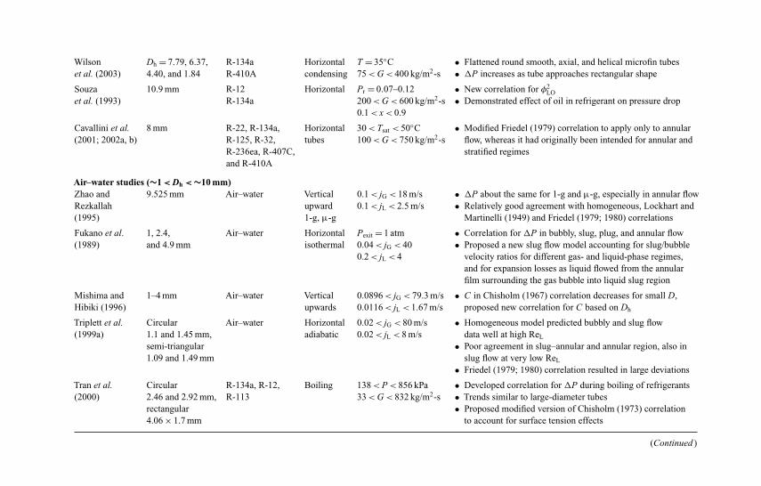
Kandlikar
I044527-Ch06.tex
26/10/200518:15
Page283
Wilson Dh = 7.79, 6.37, R-134a Horizontal T = 35◦C • Flattened round smooth, axial, and helical microfin tubeset al. (2003) 4.40, and 1.84 R-410A condensing 75<G< 400 kg/m2-s • P increases as tube approaches rectangular shape
Souza 10.9 mm R-12 Horizontal Pr = 0.07–0.12 • New correlation for φ2LO
et al. (1993) R-134a 200<G< 600 kg/m2-s • Demonstrated effect of oil in refrigerant on pressure drop0.1< x< 0.9
Cavallini et al. 8 mm R-22, R-134a, Horizontal 30<Tsat < 50◦C • Modified Friedel (1979) correlation to apply only to annular(2001; 2002a, b) R-125, R-32, tubes 100<G< 750 kg/m2-s flow, whereas it had originally been intended for annular and
R-236ea, R-407C, stratified regimesand R-410A
Air–water studies (∼1 < Dh < ∼10 mm)Zhao and 9.525 mm Air–water Vertical 0.1< jG < 18 m/s • P about the same for 1-g and µ-g, especially in annular flowRezkallah upward 0.1< jL < 2.5 m/s • Relatively good agreement with homogeneous, Lockhart and(1995) 1-g, µ-g Martinelli (1949) and Friedel (1979; 1980) correlations
Fukano et al. 1, 2.4, Air–water Horizontal Pexit = 1 atm • Correlation for P in bubbly, slug, plug, and annular flow(1989) and 4.9 mm isothermal 0.04< jG < 40 • Proposed a new slug flow model accounting for slug/bubble
0.2< jL < 4 velocity ratios for different gas- and liquid-phase regimes,and for expansion losses as liquid flowed from the annularfilm surrounding the gas bubble into liquid slug region
Mishima and 1–4 mm Air–water Vertical 0.0896< jG < 79.3 m/s • C in Chisholm (1967) correlation decreases for small D,Hibiki (1996) upwards 0.0116< jL < 1.67 m/s proposed new correlation for C based on Dh
Triplett et al. Circular Air–water Horizontal 0.02< jG < 80 m/s • Homogeneous model predicted bubbly and slug flow(1999a) 1.1 and 1.45 mm, adiabatic 0.02< jL < 8 m/s data well at high ReL
semi-triangular • Poor agreement in slug–annular and annular region, also in1.09 and 1.49 mm slug flow at very low ReL
• Friedel (1979; 1980) correlation resulted in large deviations
Tran et al. Circular R-134a, R-12, Boiling 138<P< 856 kPa • Developed correlation for P during boiling of refrigerants(2000) 2.46 and 2.92 mm, R-113 33<G< 832 kg/m2-s • Trends similar to large-diameter tubes
rectangular • Proposed modified version of Chisholm (1973) correlation4.06 × 1.7 mm to account for surface tension effects
(Continued )

Kandlikar
I044527-Ch06.tex
26/10/200518:15
Page284
Table 6.3(Continued )
Hydraulic Orientation/ Range/Investigator diameter (mm) Fluids conditions applicability Techniques, basis, observations
Zhao and Bi Equilateral Air–water Vertical 0.1< jG < 100 m/s • Frictional P correlated using Lockhart and Martinelli(2001b) triangular upward For Dh = 2.886, (1949) approach
channels co-current 1.443 mmDh = 0.866, 0.08< jL < 6 m/s1.443, and For Dh = 0.866 mm2.886 mm 0.1< jL < 10 m/s
Lee and Rectangular Air–water Horizontal 175<ReLO < 17700 • Commented on weaker coupling between phases in smallerLee (2001) 20 mm wide 0.303<X < 79.4 channels, correlated parameter C in the two-phase multiplier
Gap 0.4–4 mm (Chisholm, 1967) in terms of non-dimensional parametersto include surface tension effects
Condensation studies (∼0.4 < Dh < ∼5 mm)Yang and Rectangular R-12 Horizontal 400<G< 1400 kg/m2-s • P in microfin tube higher than in plain tubeWebb (1996b) plain: Dh = 2.64, adiabatic 0.1< x< 0.9 • Equivalent Re-based model for P
Microfin: Dh = 1.56 • Concluded surface tension does not affect P
Yan and 2 mm R-134a Horizontal T = 40–50◦C • Used Akers et al. (1959) equivalent mass velocity conceptLin (1999) to correlate condensation P

Kandlikar
I044527-Ch06.tex
26/10/200518:15
Page285
Zhang and 3.25 and 6.25 mm R-134a, R-22 Adiabatic T = 20–65◦C • Friedel (1979; 1980) correlation did not predict data wellWebb (2001) Multiport R-404A 200<G< 1000 kg/m2-s • P function of reduced pressure rather than density or
extruded Al viscosity ratio; proposed new correlation for φ2LO
Dh = 2.13 mm
Garimella et al. 0.5–4.91 mm R-134a Horizontal T ∼ 52◦C • Flow regime based models for intermittent and(2002; 2003a, b; 0< x< 1 annular/mist/disperse flow regimes2005) 150<G< 750 kg/m2-s • Intermittent flow model treats P as combination of P due
to liquid slug, film–bubble interface, and transitions betweenslug and bubble, slug frequency deduced from P data
• Annular flow model: interfacial friction factor derived frommeasured pressure drops correlated with ReL, fL, X , andsurface tension parameter
• Combined model ensures smooth transitions across regimesAir–Water Studies (Dh < ∼500 µm)Kawahara et al. 100 µm Nitrogen–water Horizontal 0.1< jG < 60 m/s • Homogeneous correlations did not predict data well(2002) 0.02< jL < 4 m/s • Lockhart and Martinelli (1949) approach with Chisholm
(1967) coefficient significantly overpredicted data• Proposed new values for parameter C based on data
Chung and 530, 250, Nitrogen–water Horizontal T = 22.9–29.9◦C • Effect of diameter investigatedKawaji (2004) 100, and 50 µm 0.02< jG < 72.98 m/s • New slug flow model based on work of Garimella et al.
0.01< jL < 5.77 m/s (2002; 2003a, b; 2005) for 50- and 100-µm tubes

Kandlikar I044527-Ch06.tex 26/10/2005 18: 15 Page 286
286 Heat transfer and fluid flow in minichannels and microchannels
6.4.1. Classical correlations
Pressure drops in conventional channels have long been calculated using three well-knowncorrelations by Lockhart and Martinelli (1949), Chisholm (1973), and Friedel (1979;1980), sometimes with modifications to account for the specific geometry or flow con-ditions under investigation. The Lockhart–Martinelli (1949) correlation was based onadiabatic flow of air and benzene, kerosene, water, and various oils flowing through 1.5–26-mm pipes, and the pressure drops were correlated based on whether the individualliquid and gas phases were considered to be in laminar or turbulent flow. As many of theseparated flow correlations for small channels are also based on this basic methodology,a brief overview is presented here. The two-phase pressure drop is expressed in terms oftwo-phase multipliers to the corresponding single-phase liquid or gas-phase pressure drop:
φ2L = (dPF /dz)
(dPF /dz)L(6.36)
φ2G = (dPF /dz)
(dPF /dz)G(6.37)
φ2LO = (dPF /dz)
(dPF /dz)LO(6.38)
where φ2 is the two-phase multiplier, the subscripts L and G refer to the flow of the liquidand gas phases flowing through the whole channel, and LO refers to the entire fluid flowoccurring as a liquid phase through the channel. These multipliers are in turn most often
correlated in terms of the Martinelli parameter X =[(dPF /dz)L(dPF /dz)G
]0.5(which has been referred
to in the previous sections). Chisholm (1967) developed the following correlations for thetwo-phase multipliers of Lockhart and Martinelli:
φ2L = 1 + C
X+ 1
X 2 (6.39)
φ2G = 1 + CX + X 2 (6.40)
where C depends on the flow regime of the liquid and gas phases. While these (Lockhartand Martinelli, 1949; Chisholm, 1967) correlations have shown considerable deviationsfrom the data for small channels with phase-change flows, they continue to be the basisfor many of the more recent correlations, as will be seen later in this section.
Chisholm (1973) modified the procedure and equations developed by Baroczy (Baroczyand Sanders, 1961; Baroczy, 1966) that account for fluid properties, quality, and mass fluxbased on steam, water/air, and mercury/nitrogen data to develop the following correlation:
φ2LO = 1 + (
Y 2 − 1)
[Bx(2−n)/2 (1 − x)(2−n)/2 + x2−n] (6.41)

Kandlikar I044527-Ch06.tex 26/10/2005 18: 15 Page 287
Chapter 6. Condensation in minichannels and microchannels 287
where n is the exponent for Reynolds number in the turbulent single-phase friction factorcorrelation, for example, n = 0.5 for the Blasius equation. The parameter Y is the Chisholmparameter:
Y =[(dPF /dz)GO
(dPF /dz)LO
]0.5
(6.42)
and B is given by:
B = 55
G0.5 0 < Y < 9.5
= 520(YG0.5
) 9.5 < Y < 28
= 15,000(Y 2G0.5
) 28 < Y
(6.43)
Friedel (1979; 1980) developed the following correlation based on a database of 25,000points for adiabatic flow through channels with d > 1 mm:
φ2LO = E + 0.324FH
Fr0.045We0.035 (6.44)
where
E = (1 − x)2 + x2(ρL fGO
ρG fLO
)(6.45)
F = x0.78 (1 − x)0.24 (6.46)
H =(ρL
ρG
)0.91 (µG
µL
)0.19 (1 − µG
µL
)0.7
(6.47)
and Fr = G2/gDρ2TP and We = G2D/ρTPσ, and fLO and fGO are the single-phase friction
factors for the total fluid flow occurring as liquid and gas respectively. The two-phasemixture density is calculated as follows:
ρTP =(
x
ρG+ 1 − x
ρL
)−1
(6.48)
The above correlation is the more widely used correlation for vertical upward and horizontalflow, and is recommended by Hewitt et al. (1994) for situations where surface tension dataare available, and by Hetsroni (1982) for µl/µv < 1000.
While these correlations have been used widely, often their predictive capabilities arenot particularly good, primarily because investigators have tried to use them beyond theiroriginally intended range of applicability, and also because these models do not account forthe flow regimes that are established over these diverse ranges of conditions and geometries.

Kandlikar I044527-Ch06.tex 26/10/2005 18: 15 Page 288
288 Heat transfer and fluid flow in minichannels and microchannels
6.4.2. Condensation or adiabatic liquid–vapor studies (∼2<Dh <∼10 mm)
Hashizume et al. (1985) conducted flow visualization and pressure drop experimentson refrigerants R-12 and R-22 flowing through horizontal 10-mm tubes over the range20◦C<T< 50◦C. They developed pressure drop expressions for annular and stratifiedflow, describing the liquid- and gas-phase velocity profiles in terms of the Prandtl mixinglength. The pressure drop was modeled as dP/dL = (4(Re+)2µ2
L/ρLD3) where Re+ is thefriction Reynolds number. Stratified flow was modeled as flow between parallel plates withthe liquid pool forming one of the parallel plates, with an equivalent gap between the platesderived in terms of the tube diameter, quality, and mass flux. Transition (wavy) region pres-sure drops were calculated by interpolating between the annular and stratified regions,with the corresponding transitions established by the modified Baker map developedby them (Hashizume, 1983). They later (Hashizume and Ogawa, 1987) tried to extendthis work to air–water and steam–water flows, but found that the best agreement was withrefrigerant data, and not with air–water or steam–water mixtures.
Wang et al. (1997b) measured pressure drops during the adiabatic flow of refrigerantsR-22, R-134a, and R-407C in a 6.5-mm tube for the mass flux range 50<G< 700 kg/m2-s.They computed two-phase multipliers φ2
G analogous to the Lockhart–Martinelli (1949)correlation from the measured pressure drops, and tried to obtain the best fit for the Cparameter in Chisholm’s (1967) equation for the multiplier, because they found that C wasstrongly dependent on the flow pattern. For R-22 and R-134a, the intermittent flow datawere predicted well with C = 5. For G> 200 kg/m2-s, wavy-annular flow was observedwith the two-phases being turbulent, and the multipliers did not depend on the mass flux.For G = 50 and 100 kg/m2-s, there was a pronounced influence of the mass flux. Theystated that for G = 100 kg/m2-s, the flow is not shear dominated, thus the waves do notreach the top of the tubes, and the pressure drop would therefore depend on the wettedperimeter, which in turn depends on the mass flux. However, for G> 200 kg/m2-s, eventhough the flow continues to be wavy (with a thicker film at the bottom), the waves do reachthe top of the tube and render the tube completely wet, which makes the wetted perimeterrelatively constant as the mass flux varies. Based on these considerations, they developedthe following equations for the two-phase multiplier:
For G> 200 kg/m2-s:
φ2G = 1 + 9.4X 0.62 + 0.564X 2.45 (6.49)
and for G< 200 kg/m2-s, the C parameter in the Chisholm (1967) correlation for theLockhart–Martinelli (1949) multiplier was modified to include a mass flux dependence asfollows:
C = 4.566 × 10−6X 0.128Re0.938LO
(ρL
ρG
)−2.15 (µL
µG
)5.1
(6.50)
Hurlburt and Newell (1999) developed scaling equations for condensing flows that wouldenable the prediction of void fraction, pressure drop, and heat transfer for a refrigerant at agiven condition and tube diameter from the available results for another similar fluid (R-11,

Kandlikar I044527-Ch06.tex 26/10/2005 18: 15 Page 289
Chapter 6. Condensation in minichannels and microchannels 289
R-12, R-22, and R-134a) operating at a different condition in the diameter range 3–10 mm.To achieve this, they assumed that the bulk of the condensation process occurs under annularflow conditions, and that even though in reality, the condensing film is non-uniform aroundthe circumference, an equivalent average film thickness would suffice for the prediction ofshear stress. They further considered that the primary resistance to heat transfer occurs inthe viscous and buffer layers of the film, regardless of the actual thickness. The approachused for modeling the film and core flows was similar to that of Rohsenow et al. (Rohsenowet al., 1957; Bae et al., 1971; Traviss et al., 1973), assuming turbulent vapor and liquidfilms and law-of-the-wall universal velocity and temperature profiles. (The liquid film wasassumed to be turbulent even at low Re (Re > 240) due to interactions with the turbulentvapor core, based on the work of Carpenter and Colburn (1951).) They used the interfacialshear stress, rather than the void fraction, as an input to determine the liquid film thickness,which enabled them to capture the dependence of void fraction on mass flux. They usedvoid fraction, pressure drop, and heat transfer data of Sacks (1975) for R-11, R-12, andR-22, and the R-22 and R-134a data of Dobson (1994) to validate their model. Using theseconsiderations, they developed the following scaling equation for pressure drop prediction:
P2/P1 = (ρg2 /ρg1
)−0.75 (ρL2 /ρL1
)−0.25 (µg2 /µg1
)−0.15 (µL2 /µL1
)0.125
× (D2/D1)−1.0 (G2/G1)
2 (x2/x1)1.65
(1 − x2
1 − x1
)0.38
(6.51)
This equation predicts a five-fold increase in pressure drop between R-22 and R-11, primar-ily due to the drastic difference in saturation pressure at 40◦C (959 kPa for R-22, 175 kPafor R-11), which leads to a much higher vapor-phase density for R-22 (65.7 kg/m3) than forR-11 (9.7 kg/m3). This approach was considered to be valid for the quality range 0.2< x<0.8, where annular flow prevails in general. Although there were some disagreementsbetween the trends predicted by this equation and the experimental data, particularly inthe effect of mass flux, the approach provides some general guidance for the modeling ofannular flows.
Chen et al. (2001) attempted to account for the increased influence of surface tension andthe decreased influence of gravity in tubes with D< 10 mm for fluids encompassing a widerange of properties, air–water (in 1.02-, 3.17-, 5.05-, 7.02 mm tubes) and R-410A (in 3.17-,5.05-, 7.02-, 9.0 mm tubes). The air–water tests were conducted at room temperature,while the R-410A tests were conducted at 5◦C and 15◦C, somewhat lower than typicalcondensation temperatures of interest. Poor agreement was found between their pressuredrop data and the predictions of the Chisholm (1967), Friedel (1979), and homogeneousflow (with average viscosity (Beattie andWhalley, 1982)) models. Therefore, they modifiedthe homogeneous flow model by including the Bond number and the Weber number toaccount for the effects of surface tension and mass flux:
dP
dz= dP
dz
∣∣∣∣hom
�hom
�hom ={
1 + (0.2 − 0.9 exp(−Bo)) Bo < 2.51 + (
We0.2/exp(Bo0.3
))− 0.9 exp(−Bo) Bo ≥ 2.5
(6.52)
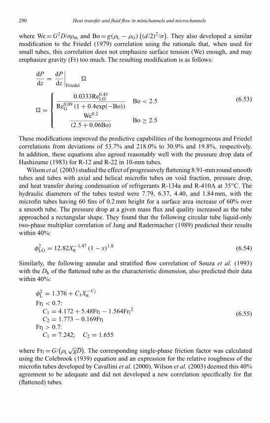
Kandlikar I044527-Ch06.tex 26/10/2005 18: 15 Page 290
290 Heat transfer and fluid flow in minichannels and microchannels
where We = G2D/σρm and Bo = g(ρL − ρG)((d/2)2/σ
). They also developed a similar
modification to the Friedel (1979) correlation using the rationale that, when used forsmall tubes, this correlation does not emphasize surface tension (We) enough, and mayemphasize gravity (Fr) too much. The resulting modification is as follows:
dP
dz= dP
dz
∣∣∣∣Friedel
�
� =
0.0333Re0.45LO
Re0.09G (1 + 0.4exp(−Bo))
Bo < 2.5
We0.2
(2.5 + 0.06Bo)Bo ≥ 2.5
(6.53)
These modifications improved the predictive capabilities of the homogeneous and Friedelcorrelations from deviations of 53.7% and 218.0% to 30.9% and 19.8%, respectively.In addition, these equations also agreed reasonably well with the pressure drop data ofHashizume (1983) for R-12 and R-22 in 10-mm tubes.
Wilson et al. (2003) studied the effect of progressively flattening 8.91-mm round smoothtubes and tubes with axial and helical microfin tubes on void fraction, pressure drop,and heat transfer during condensation of refrigerants R-134a and R-410A at 35◦C. Thehydraulic diameters of the tubes tested were 7.79, 6.37, 4.40, and 1.84 mm, with themicrofin tubes having 60 fins of 0.2 mm height for a surface area increase of 60% overa smooth tube. The pressure drop at a given mass flux and quality increased as the tubeapproached a rectangular shape. They found that the following circular tube liquid-onlytwo-phase multiplier correlation of Jung and Radermacher (1989) predicted their resultswithin 40%:
φ2LO = 12.82X −1.47
tt (1 − x)1.8 (6.54)
Similarly, the following annular and stratified flow correlation of Souza et al. (1993)with the Dh of the flattened tube as the characteristic dimension, also predicted their datawithin 40%:
φ2L = 1.376 + C1X −C2
tt
Frl < 0.7:C1 = 4.172 + 5.48Frl − 1.564Frl
2
C2 = 1.773 − 0.169FrlFrl > 0.7:
C1 = 7.242; C2 = 1.655
(6.55)
where Frl = G/(ρL
√gD). The corresponding single-phase friction factor was calculated
using the Colebrook (1939) equation and an expression for the relative roughness of themicrofin tubes developed by Cavallini et al. (2000). Wilson et al. (2003) deemed this 40%agreement to be adequate and did not developed a new correlation specifically for flat(flattened) tubes.

Kandlikar I044527-Ch06.tex 26/10/2005 18: 15 Page 291
Chapter 6. Condensation in minichannels and microchannels 291
6.4.3. Air–water studies (∼1<Dh <∼10 mm)
Zhao and Rezkallah (1995) measured pressure drops for upward air–water flow data in a9.5-mm tube at 1-g and microgravity conditions and found that the pressure drops wereabout the same at both environments. In addition, the data were in relatively good agree-ment with the homogeneous, Lockhart–Martinelli (1949) and Friedel (1979) correlations,although Friedel’s correlation was found to overestimate the data. They reasoned that atreduced gravity, annular flow pressure drops would not be affected due to the dominanceof inertia forces. In bubble and slug flows, the slip between the two phases decreases due toa decrease in gas-phase velocity, leading to a higher void fraction, and therefore increasingthe liquid phase pressure drop due to the reduced liquid flow area. However, in bubbly flow,the decrease in turbulence at reduced gravity due to the similar velocities of the gas and liq-uid phases would lead to lower pressure drops. The difference in pressure drop at 1-g andµ-g would be due to a trade-off between these competing influences. However, at therelatively high velocities and fully turbulent flows they tested, small changes in bubblevelocity due to the change in gravity were not deemed to be very significant in altering thepressure drop.
Fukano et al. (1989) proposed correlations for pressure drop in bubbly, slug, plug, andannular flow based on experiments with air–water flow in 1-, 2.4-, and 4.9-mm tubes.In slug flow, sequential photographs showed that the velocity of the large gas bubblecan be correlated as uS = 1.2 ( jG + jL) where jG + jL is the liquid slug velocity. Fromthis, the relative velocity between the gas bubble and the liquid in the slug is given byur = 0.2 ( jG + jL). From photographic observations, it was also established that the liquidslug length is given by:
LL/(LL + LG) = KjL/( jL + jG) (6.56)
where the constant of proportionality K varied from 0.9 at 1 mm to 0.72 at 4.9 mm. Assum-ing that in slug and plug flows, the pressure drop occurs in the liquid slug only, while inannular and bubbly regions, it occurs over the entire length of the channel, they developedthe following equations for the two-phase multiplier:
φ2L ∝ K
(ρT
ρL
)(νL
νT
)n ( jG + jLjL
)n+c+1
Ren−mL (6.57)
where c = 0 for intermittent flow and c = 1 for annular and bubbly flows, subscript T refersto the two-phase mixture, and m and n refer to the Re exponent in the single-phase frictionfactor for the liquid and two-phase flows, respectively, dependent on whether the flow islaminar or turbulent. As the experimental φ2
L values were larger than those predicted bythis treatment, they proposed a new slug flow model that accounts for the expansion losses(loss coefficient = 1) as the liquid flowed from the annular film surrounding the gas bubbleinto the liquid slug region. This additional contribution of the expansion losses was shownto be significant, and led to much better agreement between the measured and predictedvalues. The analysis also showed that for a 2.4-mm channel, the expansion losses couldin fact be larger than the frictional losses in the slug. The expansion losses were foundto first increase with increasing jG because the liquid slug length decreases, presumably

Kandlikar I044527-Ch06.tex 26/10/2005 18: 15 Page 292
292 Heat transfer and fluid flow in minichannels and microchannels
leading to more expansion events; but further increases in jG make the expansion lossesless significant because at very high jG, the frictional losses increase rapidly.
Mishima and Hibiki (1996) (whose work was discussed in the previous sections on flowregimes and void fraction) measured frictional pressure drops in air–water flows through1–4-mm tubes. By comparing their results with the Lockhart–Martinelli (1949) correlation,they noticed that the parameter C in Chisholm’s (1967) curve-fit (Eq. (6.39) above) to themultiplier decreased with a decrease in tube diameter. Similar trends were also observedby Sugawara et al. (1967) for air–water flow in horizontal 0.7–9.1-mm round tubes, Ungarand Cornwell (1992) for the flow of ammonia in horizontal 1.46–3.15-mm round tubes,Mishima et al. (1993) for vertical upward flow of air–water in rectangular 1.07 × 40-,2.45 × 40-, and 5.00 × 40-mm channels, Sadatomi et al. (1982) for vertical upward flow ofair–water through rectangular (7–17) × 50- and 7 × 20.6-mm channels, and by Moriyamaet al. (1992a,b) for the flow of R113-nitrogen through horizontal rectangular (0.007–0.098) × 30-mm channels. Including the data from these investigators and their own data,they developed the following equation for the parameter C:
C = 21(1 − exp(−0.319Dh)) (6.58)
where Dh is in mm. They state that this equation is valid for vertical and horizontal roundtubes as well as rectangular ducts (although the predictions did not agree well with theammonia vapor data of Ungar and Cornwell (1992)).
It should be noted that several investigators have shown that the homogeneous flowmodel is reasonably successful in predicting pressure drop during adiabatic flow and boilingin channels with a diameter of a few mm. These include the previously mentioned workof Ungar and Cornwell (1992) on the flow of ammonia in horizontal 1.46–3.15-mm roundtubes, and Kureta et al. (1998) on the boiling of water in 2–6-mm channels at atmosphericpressure over a wide range of mass fluxes. Similarly, Triplett et al. (1999a) found that thismodel was able to predict some of their data on adiabatic flow of air–water mixtures through1.1- and 1.45-mm circular, and 1.09- and 1.49-mm semi-triangular channels. In particular,the homogeneous model predicted the data in the bubbly and slug flow regimes well athigh ReL. The agreement in the slug-annular and annular flow regions was poor, as wasthe agreement with the slug flow data at very low ReL. Also, the Friedel (1979) correlationresulted in larger deviations from the data, especially at low ReL values. This same group(Ekberg et al., 1999) also investigated air–water flow in two narrow, concentric annuli withinner and outer diameters of 6.6 and 8.6 mm for one annulus, and 33.2 and 35.2 mm forthe second annulus, respectively. The measured pressure drops did not show particularlygood agreement with any of the available models, and even the Friedel correlation, whichthey state provided the best agreement, had deviations of over 50%.
Tran et al. (2000) developed a correlation for pressure drop during boiling of refrigerantsin circular (2.46 and 2.92 mm) and rectangular (4.06 × 1.7 mm) channels. Their tests didnot record local pressure drops – the pressure drop was measured from the inlet at nominallyzero quality to a varying exit quality. For the tests with large exit qualities, therefore, themeasured pressure drops could be the result of considerably varying local pressure dropsas the flow regimes change along the test section. Although they found that the trends inthe data (in terms of the effect of mass flux, quality and saturation pressure) were similar

Kandlikar I044527-Ch06.tex 26/10/2005 18: 15 Page 293
Chapter 6. Condensation in minichannels and microchannels 293
to those found in large tubes (Eckels et al., 1994), the large tube correlations (Chisholm,1967, 1973; Friedel, 1979; Jung and Radermacher, 1989; Souza and Pimenta, 1995)typically underpredicted the data, with the discrepancy increasing at large qualities andmass fluxes. The reason for the higher pressure drop in small tubes was thought to be thefact that coalesced bubbles in small channels are confined, elongated, and slide over a thinliquid film, whereas in large tubes, the bubbles may grow and flow unrestricted through thetubes. In view of this, they proposed a modified version of the Chisholm (1973) correlationthat accounted for the role of surface tension through the confinement number (defined ina previous section of this chapter) introduced by Cornwell and Kew (1993) as follows:
Pf = pfLO{1 + (
4.3Y 2 − 1) [
Nconf x0.875 (1 − x)0.875 + x1.75]} (6.59)
where Y is the ratio of the gas- and liquid-only pressure drops defined in Eq. (6.42) above.Zhao and Bi (2001b) measured pressure drops for upward co-current air–water flow
through equilateral triangular channels with Dh = 0.866, 1.443, and 2.886 mm. They foundthat the void fraction could be simply represented by α= 0.838β, which is very similar tothe Armand (1946) correlation and was used to compute acceleration losses in two-phaseflow. The frictional component was then correlated using the Lockhart–Martinelli (1949)approach. For this, they computed the required single-phase friction factor by replacingthe laminar and turbulent friction factors in the comprehensive laminar-transition-turbulentcorrelation of Churchill (1977) with the corresponding expressions for triangular channels.This modification yielded two-phase multipliers that were between the values predicted bythe Chisholm (1967) expression using C = 5 and C = 20.
Lee and Lee (2001) investigated pressure drop for air–water flow through 20-mm widehorizontal rectangular channels with gaps of 0.4–4 mm. They recalled that the originalbasis for the Chisholm (1967) correlation of the two-phase multiplier in the Lockhart–Martinelli (1949) correlation consisted of accounting for the pressure drop due to (a) gasphase, (b) liquid phase, and (c) interactions between the two phases. The parameter C inChisholm’s correlation represents this interaction term; which in turn depends on the flowregimes of the two phases. Therefore, they proposed different values for C, accounting forthe gap size as well as the phase flow rates. They reasoned that as the gap size decreases,the flow tends more and more to plug and slug flow, with an increasing effect of surfacetension due to the curved gas/liquid interface at the edge of the bubble. In such surface-tension-dominated flows, they stated that of the several dimensionless parameters identifiedby Suo and Griffith (1964) for capillary tubes, the Reynolds number of the liquid slug,Re = (ρL jDh)/µL, the ratio of viscous and surface tension effects, ψ = µL j/σ, and acombination of parameters independent of the liquid slug velocity, λ = µ2
L/(ρLσDh),were the relevant ones. Lee and Lee then used their data to obtain individual values of theconstant A and exponents q, r, and s for each combination of liquid and gas flow regimesin the following equation for the parameter C in the two-phase multiplier:
C = AλqψrResLO (6.60)
Regression analysis showed that the dependence on parameters λ and ψ above, that is,surface tension effects, was only significant when both phases were laminar, with C being

Kandlikar I044527-Ch06.tex 26/10/2005 18: 15 Page 294
294 Heat transfer and fluid flow in minichannels and microchannels
simply a function of ReLO when either or both phases were in the turbulent regime. Thisapproach predicted their data within ±10%, and also predicted the data of Wambsgansset al. (1992) and Mishima et al. (1993) within 15% and 20%, respectively. This correlationis valid for 175 < ReLO < 17700 and 0.303<X < 79.4.
6.4.4. Condensation studies (∼0.4<Dh < 5 mm)
Yang and Webb (1996b) measured pressure drops in single- and adiabatic two-phaseflows of refrigerant R-12 in rectangular plain and microfin tubes with Dh = 2.64 and1.56 mm, respectively. The measurements were conducted at somewhat higher mass fluxes(400<G< 1400 kg/m2-s) than those of interest for refrigeration and air-conditioningapplications. Their single-phase friction factors were correlated by fsmooth = 0.0676Re−0.22
Dh
and fmicrofin = 0.0814Re−0.22Dh
. The pressure gradient in the microfin tube was higher thanthat of the plain tube. They tried to model the two-phase pressure drops using the Lockhart–Martinelli (1949) approach and curve-fitting the two-phase multiplier φ2
v, but this did notlead to a satisfactory correlation. The equivalent mass velocity concept of Akers et al.(1959) was then attempted to develop a correlation. Thus, the single-phase friction factoris first calculated using the aforementioned equations at the Reynolds number ReDh for theliquid phase flowing alone. The equivalent Reynolds number for two-phase flow is thencalculated as follows:
Reeq = GeqDh
µl; Geq = G
[(1 − x)+ x
(ρl
ρv
)1/2]
(6.61)
The equivalent friction factor is therefore based on an equivalent all-liquid flow that yieldsthe same frictional pressure drop as the two-phase flow. Based on their data, the two-phasefriction factor at this equivalent Reynolds number was fit to the following equation:
f
fl= 0.435Re0.12
eq (6.62)
Finally, the two-phase pressure drop is calculated as follows:
Pf = fRe2
eqµ2l
2ρl
4L
D3h
(6.63)
This approach was able to predict both plain and microfin tube data within ±20%. It shouldbe noted that this approach collapses both the single- and two-phase pressure gradients foreach tube on the same line, when plotted against the Reeq. From their data, Yang and Webb(1996b) also concluded that surface tension did not play a role in determining the pressuredrop in these tubes, although in related work (Yang and Webb, 1996a), they found surfacetension to be significant for the heat transfer coefficient, especially at low G and high x.
Subsequently, Yan and Lin (1999) used the same Akers et al. (1959) equivalent massvelocity concept that was used by Yang and Webb (1996b) to correlate condensation
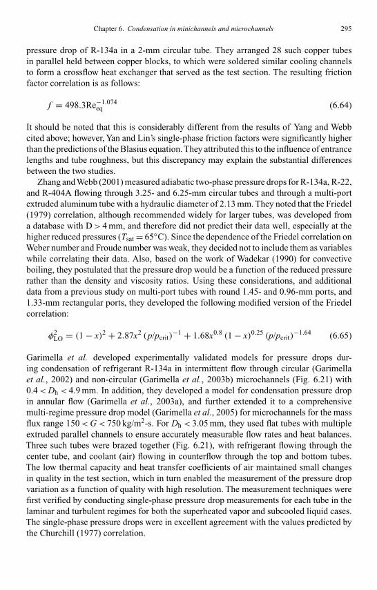
Kandlikar I044527-Ch06.tex 26/10/2005 18: 15 Page 295
Chapter 6. Condensation in minichannels and microchannels 295
pressure drop of R-134a in a 2-mm circular tube. They arranged 28 such copper tubesin parallel held between copper blocks, to which were soldered similar cooling channelsto form a crossflow heat exchanger that served as the test section. The resulting frictionfactor correlation is as follows:
f = 498.3Re−1.074eq (6.64)
It should be noted that this is considerably different from the results of Yang and Webbcited above; however, Yan and Lin’s single-phase friction factors were significantly higherthan the predictions of the Blasius equation. They attributed this to the influence of entrancelengths and tube roughness, but this discrepancy may explain the substantial differencesbetween the two studies.
Zhang and Webb (2001) measured adiabatic two-phase pressure drops for R-134a, R-22,and R-404A flowing through 3.25- and 6.25-mm circular tubes and through a multi-portextruded aluminum tube with a hydraulic diameter of 2.13 mm. They noted that the Friedel(1979) correlation, although recommended widely for larger tubes, was developed froma database with D> 4 mm, and therefore did not predict their data well, especially at thehigher reduced pressures (Tsat = 65◦C). Since the dependence of the Friedel correlation onWeber number and Froude number was weak, they decided not to include them as variableswhile correlating their data. Also, based on the work of Wadekar (1990) for convectiveboiling, they postulated that the pressure drop would be a function of the reduced pressurerather than the density and viscosity ratios. Using these considerations, and additionaldata from a previous study on multi-port tubes with round 1.45- and 0.96-mm ports, and1.33-mm rectangular ports, they developed the following modified version of the Friedelcorrelation:
φ2LO = (1 − x)2 + 2.87x2 (p/pcrit)
−1 + 1.68x0.8 (1 − x)0.25 (p/pcrit)−1.64 (6.65)
Garimella et al. developed experimentally validated models for pressure drops dur-ing condensation of refrigerant R-134a in intermittent flow through circular (Garimellaet al., 2002) and non-circular (Garimella et al., 2003b) microchannels (Fig. 6.21) with0.4<Dh < 4.9 mm. In addition, they developed a model for condensation pressure dropin annular flow (Garimella et al., 2003a), and further extended it to a comprehensivemulti-regime pressure drop model (Garimella et al., 2005) for microchannels for the massflux range 150<G< 750 kg/m2-s. For Dh < 3.05 mm, they used flat tubes with multipleextruded parallel channels to ensure accurately measurable flow rates and heat balances.Three such tubes were brazed together (Fig. 6.21), with refrigerant flowing through thecenter tube, and coolant (air) flowing in counterflow through the top and bottom tubes.The low thermal capacity and heat transfer coefficients of air maintained small changesin quality in the test section, which in turn enabled the measurement of the pressure dropvariation as a function of quality with high resolution. The measurement techniques werefirst verified by conducting single-phase pressure drop measurements for each tube in thelaminar and turbulent regimes for both the superheated vapor and subcooled liquid cases.The single-phase pressure drops were in excellent agreement with the values predicted bythe Churchill (1977) correlation.
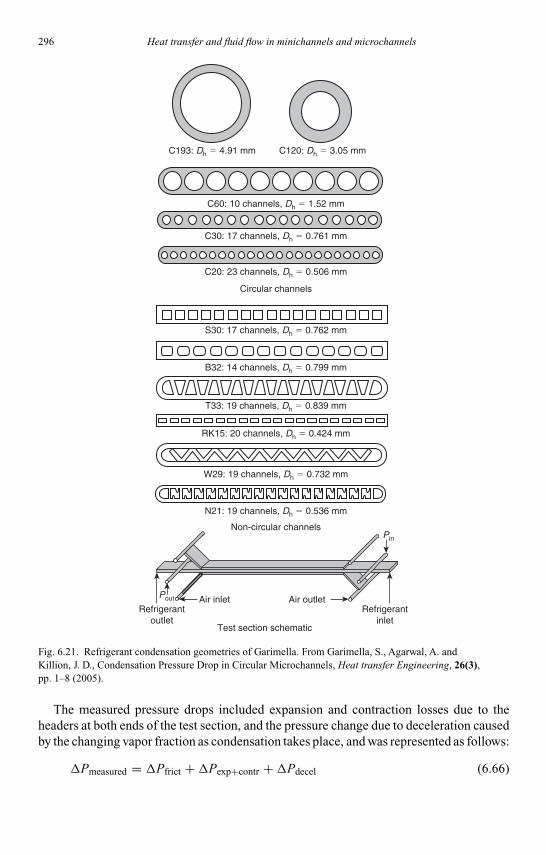
Kandlikar I044527-Ch06.tex 26/10/2005 18: 15 Page 296
296 Heat transfer and fluid flow in minichannels and microchannels
C193: Dh � 4.91 mm C120: Dh � 3.05 mm
C60: 10 channels, Dh � 1.52 mm
C30: 17 channels, Dh � 0.761 mm
C20: 23 channels, Dh � 0.506 mm
S30: 17 channels, Dh � 0.762 mm
B32: 14 channels, Dh � 0.799 mm
T33: 19 channels, Dh � 0.839 mm
RK15: 20 channels, Dh � 0.424 mm
W29: 19 channels, Dh � 0.732 mm
N21: 19 channels, Dh � 0.536 mm
Circular channels
Non-circular channels
Air inlet Air outletRefrigerant
outletRefrigerant
inletTest section schematic
Pout
Pin
Fig. 6.21. Refrigerant condensation geometries of Garimella. From Garimella, S., Agarwal, A. andKillion, J. D., Condensation Pressure Drop in Circular Microchannels, Heat transfer Engineering, 26(3),pp. 1–8 (2005).
The measured pressure drops included expansion and contraction losses due to theheaders at both ends of the test section, and the pressure change due to deceleration causedby the changing vapor fraction as condensation takes place, and was represented as follows:
Pmeasured = Pfrict +Pexp+contr +Pdecel (6.66)

Kandlikar I044527-Ch06.tex 26/10/2005 18: 15 Page 297
Chapter 6. Condensation in minichannels and microchannels 297
The pressure drop due to contraction was estimated using a homogeneous flow modelrecommended by Hewitt et al. (1994):
Pcontr = G2
2ρL
[(1
Cc− 1
)2
+ 1 − γ2
][1 + x
(ρL
ρG− 1
)](6.67)
where γ is the area ratio (Atest−section/Aheader) and Cc is the coefficient of contraction, whichis in turn a function of this area ratio as given by Chisholm (1983):
Cc = 1
0.639(1 − γ)0.5 + 1(6.68)
For the expansion into the header from the test section, the following separated flow modelrecommended by Hewitt et al. (1994) was used:
Pexpansion = G2γ (1 − γ)ψS
ρL(6.69)
where ψS, the separated flow multiplier, is also a function of the phase densities and thequality. These estimates were validated using pressure drop measurements on a “near-zero” length test section, in which the measured pressure drops (with small frictionalpressure drops) showed excellent agreement with the contraction/expansion contributionscalculated as shown above. Contraction and expansion loss contributions were less than5% of the total measured pressure drop for all their data. The pressure change due toacceleration (deceleration) of the fluid (due to the change in quality across the test section)was estimated as follows (Carey, 1992):
Pacceleration =[
G2x2
ρVα+ G2(1 − x)2
ρL(1 − α)
]x=xout
−[
G2x2
ρVα+ G2(1 − x)2
ρL(1 − α)
]x=xin
(6.70)
where the void fraction was evaluated using the Baroczy (1965) correlation. For almostall their data, the deceleration term was extremely small compared to the overall pressuredrop. These estimates were also corroborated by adiabatic flow and condensation tests atthe same nominal conditions. The residual frictional component of the two-phase pressuredrop, which generally was at least an order of magnitude larger than these minor losses, wasused for developing condensation pressure drop models for the respective flow regimes.
To develop flow regime-based pressure drop models, transition from the intermittent tothe other flow regimes (based on their earlier flow visualization work) was determined asfollows:
x ≤ a
G + b(6.71)
where a and b are geometry-dependent constants given by:
a = 69.57 + 22.60 × exp(0.259 × Dh) (6.72)

Kandlikar I044527-Ch06.tex 26/10/2005 18: 15 Page 298
298 Heat transfer and fluid flow in minichannels and microchannels
b = −59.99 + 176.8 × exp(0.383 × Dh) (6.73)
where Dh is in mm. On a mass-flux versus quality map, these transition lines appear in thelower left corner, as shown in Fig. 6.22. For pressure drop model development, they broadlycategorized the flow into the primary regimes, intermittent (lower left) and annular film/mist/disperse patterns of the annular flow regime (upper right). The very few data that werein the wavy regime in these small channels were incorporated into the annular or intermit-tent regimes, as appropriate. The overlap region in Fig. 6.22 accounts for the gradual transi-tion between the primary regimes, during which the flow switches back and forth betweenthe respective regimes. Pressure drop models for these regimes are described below.
The unit cell for the development of the intermittent model is shown in Fig. 6.23, inwhich the vapor-phase travels as long solitary bubbles surrounded by an annular liquid film
800
600
400
0.0 0.1 0.2 0.3 0.4 0.5Vapor quality (x)
Inte
rmitt
ent f
low
mod
el
Mist/annular/disperseflow model
Mas
s flu
x G
, (kg
/m2 -
s)
Overlap zone
0.6 0.7 0.8 0.9 1.0
200
0.5 mm0.76 mm1.5 mm3.0 mm4.91 mm
Fig. 6.22. Flow regime assignment. From Garimella, S., Agarwal, A. and Killion, J. D., Condensation PressureDrop in Circular Microchannels, Heat transfer Engineering, 26(3), pp. 1–8 (2005).
Lbubble
Ububble
U film
U film
DbubbleDh
Film–slugtransitionregion
Liquid Vapor
Lslug
Uslug
Fig. 6.23. Unit cell for intermittent flow. Reprinted from Garimella, S., Killion, J. D. and Coleman, J. W.An experimentally validated model for two-phase pressure drop in the intermittent flow regime for circularmicrochannels, Journal of Fluids Engineering, 124(1), pp. 205–214 (2002) with permission from the AmericanSociety of Mechanical Engineers.

Kandlikar I044527-Ch06.tex 26/10/2005 18: 15 Page 299
Chapter 6. Condensation in minichannels and microchannels 299
and separated by liquid slugs. Based on the recorded flow patterns, it was assumed that thebubble is cylindrical, and that there is no entrainment of vapor in the slug, or liquid inthe bubble. Further, for any given condition, it was assumed that the length/frequency/speedof bubbles/slugs is constant, with no bubble coalescence, and a smooth bubble/film inter-face. The total pressure drop for this flow pattern includes contributions from: the liquidslug, the vapor bubble, and the flow of liquid between the film and slug as follows:
Ptotal = Pslug +Pf/b +Ptransitions (6.74)
A simple control volume analysis (Garimella et al., 2002; 2003b) similar to that performedby Suo and Griffith (1964) was used to calculate the liquid slug velocity from the superfi-cial phase velocities, in turn calculated from the overall mass flux and the quality. Thus,Uslug = jV + jL, which yielded the slug Reynolds number Reslug = (ρLUslugDh)/µL. ThisReslug was used to calculate the pressure gradient in the slug from an appropriate single-phase friction factor correlation from the literature. The results of several investigations(Suo and Griffith, 1964; Dukler and Hubbard, 1975; Fukano et al., 1989) discussed in thischapter suggested that Ububble = 1.2Uslug. Unlike air–water studies, where many of theseinvestigators have neglected the pressure drop in the film–bubble region, since the ratio ofthe liquid to vapor densities for R-134a is much lower (approximately 16:1 versus 850:1for air–water) as is the ratio of liquid and vapor viscosities (approximately 10:1 versus50:1), the contribution of the film/bubble region was not neglected. Based on the data,the film was assumed to be laminar, while the gas bubble was turbulent. The respectiveReynolds numbers were defined as follows:
Refilm = ρLUfilm(Dh − Dbubble)
µLRebubble = ρV(Ububble − Uinterface)Dbubble
µV(6.75)
The film flow was assumed to be driven by the combination of the pressure gradient inthe film/bubble region and shear at the film/bubble interface. The velocity profile forcombined Couette–Poiseuille flow through an annulus where the inner surface moves atthe interface velocity, Uinterface, is represented by the superposition of the pressure-drivenand the shear-driven components:
ufilm(r) =−(
dPdx
)f/b
4µL
[R2
tube − r2 − (R2
tube − R2bubble
) ln(Rtube/r)
ln(Rtube/Rbubble)
]
+ Uinterfaceln(Rtube/r)
ln(Rtube/Rbubble)(6.76)
The bubble velocity, assuming a power law profile (n = 7) is given by:
ububble(r) = (n + 1)(2n + 1)
2n2(Ububble − Uinterface)
(1 − r
Rbubble
)1/n
+Uinterface (6.77)
A shear balance at the film–bubble interface yields the interface velocity:
Uinterface = −(dP/dx)f/b
4µL(R2
tube − R2bubble) (6.78)

Kandlikar I044527-Ch06.tex 26/10/2005 18: 15 Page 300
300 Heat transfer and fluid flow in minichannels and microchannels
With a parabolic velocity profile in the film, the average film velocity can also be calculated.Also, with the film pressure gradient calculated using a single-phase friction factor for thegas phase, continuity yields:
Uslug = Ububble
(Rbubble
Rtube
)2
+ Ufilm
(1 −
(Rbubble
Rtube
)2)
(6.79)
These calculations yield 0.899<Rbubble/Rtube < 0.911; that is, the bubble diameter is∼90% of the tube diameter. With the pressure drop/length known in the slug and thefilm/bubble regions, the frictional pressure drop was calculated using the relationshipproposed by Fukano et al. (1989) for the length of the slug (Eq. (6.56)):
Pfriction only = Ltube
[(dP
dx
)f/b
(1 − Lslug
Lslug + Lbubble
)
+(
dP
dx
)slug
(Lslug
Lslug + Lbubble
)](6.80)
The remaining contribution to the total pressure drop is the loss associated with the flow ofliquid between the film and the slug. As the film moves slowly, the front of the liquid slug isconstantly taking up fluid from the film. A pressure loss is associated with the accelerationand subsequent mixing of this liquid, with the total pressure loss from these transitionsgiven byPfilm/slug transitions = NUC ×Pone transition, where NUC is the number of cells perunit length. The pressure drop for one transition is based on the force to accelerate theportion of the liquid film overtaken by the rear of the bubble from the average film velocityto the average slug velocity (Dukler and Hubbard, 1975):
Pone transition = ρL
(1 −
(Rbubble
Rtube
)2)
(Uslug − Ufilm)(Ububble − Ufilm) (6.81)
These components of the total pressure drop are shown below:
P
L=(
dP
dx
)filmbubble
(Lbubble
LUC
)+(
dP
dx
)slug
(Lslug
LUC
)+P one
transition
(NUC
L
)(6.82)
A depiction of these various contributions to the measured pressure drop for circularchannels is shown in Fig. 6.24. The number of unit cells per unit length required forclosure of the model was computed from the slug frequency ω, which was correlatedbased on slug Re and Dh:
a(Reslug
)b = ωDh
Ububble= Dh
(NUC
Ltube
)=(
Dh
LUC
)(6.83)
The coefficients a and b were fit using the difference between the measured pressuredrop and the pressure drop calculated as described above for the slug and bubble/filmregions; that is, the net pressure drop due to transitions. The correlation yielded a = 2.437,b = −0.560 for both circular and non-circular (except triangular, for which different
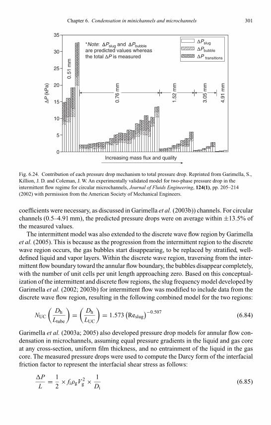
Kandlikar I044527-Ch06.tex 26/10/2005 18: 15 Page 301
Chapter 6. Condensation in minichannels and microchannels 301
∆P (
kPa)
0
5
10
15
20
25
30
35∆Pslug
∆Pbubble
∆P transitions
0.76
mm
0.51
mm
1.52
mm
3.05
mm
4.91
mm
Increasing mass flux and quality
*Note: ∆∆Pslug and ∆∆Pbubbleare predicted values whereasthe total ∆P is measured
Fig. 6.24. Contribution of each pressure drop mechanism to total pressure drop. Reprinted from Garimella, S.,Killion, J. D. and Coleman, J. W. An experimentally validated model for two-phase pressure drop in theintermittent flow regime for circular microchannels, Journal of Fluids Engineering, 124(1), pp. 205–214(2002) with permission from the American Society of Mechanical Engineers.
coefficients were necessary, as discussed in Garimella et al. (2003b)) channels. For circularchannels (0.5–4.91 mm), the predicted pressure drops were on average within ±13.5% ofthe measured values.
The intermittent model was also extended to the discrete wave flow region by Garimellaet al. (2005). This is because as the progression from the intermittent region to the discretewave region occurs, the gas bubbles start disappearing, to be replaced by stratified, well-defined liquid and vapor layers. Within the discrete wave region, traversing from the inter-mittent flow boundary toward the annular flow boundary, the bubbles disappear completely,with the number of unit cells per unit length approaching zero. Based on this conceptual-ization of the intermittent and discrete flow regions, the slug frequency model developed byGarimella et al. (2002; 2003b) for intermittent flow was modified to include data from thediscrete wave flow region, resulting in the following combined model for the two regions:
NUC
(Dh
Ltube
)=(
Dh
LUC
)= 1.573
(Reslug
)−0.507 (6.84)
Garimella et al. (2003a; 2005) also developed pressure drop models for annular flow con-densation in microchannels, assuming equal pressure gradients in the liquid and gas coreat any cross-section, uniform film thickness, and no entrainment of the liquid in the gascore. The measured pressure drops were used to compute the Darcy form of the interfacialfriction factor to represent the interfacial shear stress as follows:
P
L= 1
2× fiρgV 2
g × 1
Di(6.85)
Kandlikar I044527-Ch06.tex 26/10/2005 18: 15 Page 302
302 Heat transfer and fluid flow in minichannels and microchannels
The above equation uses the interface diameter, Di. This same expression can be repre-sented in terms of the more convenient tube diameter, D, by using the Baroczy (1965) voidfraction model:
P
L= 1
2× fi
G2 × x2
ρg × α2.5 × 1
D(6.86)
The ratio of this interfacial friction factor (obtained from the experimental data) to the cor-responding liquid-phase Darcy friction factor was then computed and correlated in termsof the Martinelli parameter and the surface tension parameter ψ= jLµL/σ introduced byLee and Lee (2001):
fifl
= A × X aRebl ψ
c (6.87)
where jL = G(1−x)ρl(1−α) is the liquid superficial velocity. The phase Reynolds numbers
required above and for the Martinelli parameter were defined in terms of the flow areas ofeach phase:
Rel = GD (1 − x)(1 + √
α)µl
Reg = GxD
µg√α
(6.88)
The friction factors were computed using f = 64/Re for Re< 2100 and the Blasius expres-sion f = 0.316 × Re−0.25 for Re> 3400. Regression analysis on data grouped into tworegions based on Rel yielded:
Laminar region (Rel < 2100): A = 1.308 × 10⁻³ a = 0.427 b = 0.930 c = −0.121
(6.89)
Turbulent region (Rel > 3400): A = 25.64 a = 0.532 b = −0.327 c = 0.021 (6.90)
Interpolations based on G and x are used to compute the pressure drop for the transitionregion. This model predicted 87% of the data within ±20%. These predictions include notonly the annular flow region, but also the mist and disperse-wave flow data, although themodel development uses a physical representation where the liquid forms an annular filmaround a gas core. Garimella et al. (2005) explained this based on the fact that the annularflow regime increases in extent for smaller tubes, causing several data classified into thewavy and mist flow regions using Dh = 1 mm transition criteria to be in fact in the annularflow regime. Representative pressure drop trends predicted by this model are shown inFig. 6.25.
6.4.5. Air–water studies (Dh <∼500µm)
Kawahara et al. (2002) measured pressure drops for air–water flow through a 100-µmcircular tube (the corresponding results on flow patterns and void fractions were discussed
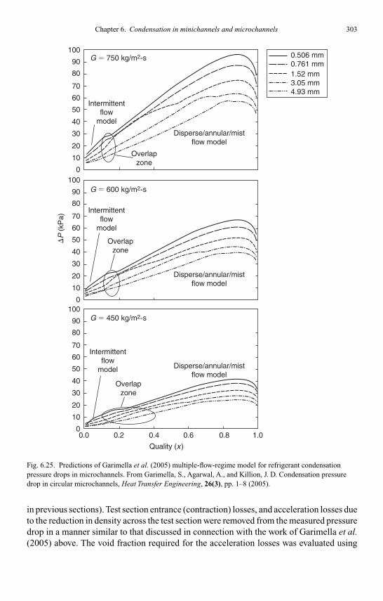
Kandlikar I044527-Ch06.tex 26/10/2005 18: 15 Page 303
Chapter 6. Condensation in minichannels and microchannels 303
100G � 750 kg/m2-s
G � 600 kg/m2-s
�P
(kP
a)
G � 450 kg/m2-s
Intermittentflow
model
Intermittentflow
model
Intermittentflow
model
Disperse/annular/mistflow model
Disperse/annular/mistflow model
Disperse/annular/mistflow model
Overlapzone
Overlapzone
Overlapzone
90
80
70
60
50
40
30
20
10
0100
90
80
70
60
50
40
30
20
10
0100
90
80
70
60
50
40
30
20
10
00.0 0.2 0.4 0.6
Quality (x)
0.8 1.0
0.506 mm0.761 mm1.52 mm3.05 mm4.93 mm
Fig. 6.25. Predictions of Garimella et al. (2005) multiple-flow-regime model for refrigerant condensationpressure drops in microchannels. From Garimella, S., Agarwal, A., and Killion, J. D. Condensation pressuredrop in circular microchannels, Heat Transfer Engineering, 26(3), pp. 1–8 (2005).
in previous sections). Test section entrance (contraction) losses, and acceleration losses dueto the reduction in density across the test section were removed from the measured pressuredrop in a manner similar to that discussed in connection with the work of Garimella et al.(2005) above. The void fraction required for the acceleration losses was evaluated using

Kandlikar I044527-Ch06.tex 26/10/2005 18: 15 Page 304
304 Heat transfer and fluid flow in minichannels and microchannels
Eq. (6.35) developed from their image analysis work. The contributions of these contractionand acceleration losses to the total pressure drop were found to be 0.05–9% and 0–4.5%,respectively, of the measured pressure drop. Although their flow pattern and void fractionresults showed that the flow was not well represented by a homogeneous model, based onthe success of others in using this model for small channels (Ungar and Cornwell, 1992;Triplett et al., 1999a), they compared their results with homogeneous model using thehomogeneous density and homogeneous viscosity models of Owens (1961), McAdams(1954), Cicchitti et al. (1960), Dukler et al. (1964), Beattie and Whalley (1982), and Linet al. (1991). They found that none of these models were able to predict their data adequately(the Dukler et al. (1964) model, µH =βµG + (1 −β)µL, provided somewhat reasonablepredictions). When a Lockhart–Martinelli (1949) type two-phase multiplier approach wasused, the Chisholm (1967) coefficient of C = 5 significantly overpredicted the data, whilea C value of 0.66 from Mishima and Hibiki’s (1996) work resulted in a 10% overprediction,and agreement within ± 10% was achieved using Lee and Lee’s (2001) correlation for C.Therefore, they conducted a regression analysis of the data to obtain a value of C = 0.24,which also yielded a ± 10% agreement. In later work on a 96 µm square channel (Chunget al., 2004), they noted that channel shape did not have any appreciable effect on two-phase pressure drop, and provided revised values of C = 0.22 for circular channels andC = 0.12 for square channels for the C coefficient in Chisholm’s (1967) model.
Chung and Kawaji (2004) also investigated the effects of channel diameter on pressuredrop during adiabatic flow of nitrogen–water through 530-, 250-, 100-, and 50 µm circularchannels. In this study, they found that the Dukler et al. (1964) viscosity model (when usedassuming homogeneous flow) did not predict the pressure drops for the 530- and 250-µmchannels, although the agreement was within ±20% for the 100- and 50-µm data. Beattieand Whalley’s (1982) mixture viscosity model showed the opposite trends, succeedingsomewhat in predicting the 530- and 250-µm channel data, but significantly overpredictingthe 100- and 50-µm channel data. They attributed this to the fact that Beattie and Whalley’s(1982) model yields a higher mixture viscosity than that of Dukler et al. (1964), resultingin better agreement with the larger channel data because of the additional mixing lossesin the bubbly and churn flows in these channels. When predominated by the more laminarslug flow with weak momentum coupling of the phases, however, as is the case in thesmaller channels, the lower viscosities predicted by Dukler et al. (1964) model are moreappropriate. When attempting the use of a two-phase multiplier approach as discussedabove, they noted a mass flux effect on the friction multiplier for the 530- and 250-µmchannels. The data at different mass fluxes for the 100- and 50-µm channels, however,were predicted well by a single C value (C = 0.22 for 100 µm, C = 0.15 for 50 µm). Thisdecrease in C value (based on the above discussion of Lee and Lee’s (2001) work) with adecrease in channel diameter implies a decrease in momentum coupling of the two phases;that is, completely separated laminar flow of gas and liquid, as also noted byAli et al. (1993).
Based on the somewhat inadequate predictions of the homogeneous and two-phasemultiplier approaches, they adapted the intermittent flow model of Garimella et al. (2002)to calculate the pressure drops in the 50- and 100-µm channels, which have predomi-nantly intermittent flows. They also used the unit-cell concept consisting of gas bubblessurrounded by a liquid film and flowing through slower moving liquid slugs. Although inaccordance with the model of Garimella et al. (2002), they represented the total pressure
Kandlikar I044527-Ch06.tex 26/10/2005 18: 15 Page 305
Chapter 6. Condensation in minichannels and microchannels 305
drop as the summation of the frictional pressure drop in each of these regions, they ignoredthe mixing losses at the transitions between these regions. The rationale used was that inthese smaller channels, the liquid flow is typically laminar, with suppressed mixing lead-ing to negligibly small transition losses. For the single-phase liquid region, they computedthe average liquid velocity UL = jL/(1 −α), which yielded ReL = (ρLULD)/µL. Laminaror turbulent single-phase friction factors were calculated based on ReL. To compute thepressure drop in the film/bubble region, they assumed the average velocity of the gas phaseand the gas bubble to be equal, UG = UB, where UG = jG/α. This assumption is differentfrom the assumption by Garimella et al. (2002) that UB = 1.2US, which, according toChung and Kawaji (2004), is equivalent to assuming that the Armand (1946) correlationfor void fraction approximately holds. Instead, they used the nonlinear expression for voidfraction derived by them and discussed here in the previous section. Defining the bubbleReB in terms of the relative velocity between the bubble and the interface, the computa-tion of the pressure drop in the film–bubble region develops much like that in Garimellaet al. (2002), with an assumption that DB = 0.9D. The interface velocity, the film–bubblepressure gradient, and the bubble Reynolds number are then obtained iteratively. To cal-culate the relative lengths of the bubble and slug regions, they relied on the void fractionmeasured by them. Thus, treating the bubble as a cylinder with flat ends, the bubble lengthis given by:
LB
LUC= α
(D
DB
)2
(6.91)
Finally, the total pressure drop in the two regions is given by:
(dPf
dz
)TP
=(
dP
dz
)F/B
LB
LUC+(
dP
dz
)L
LL
LUC(6.92)
The model was shown to agree better with the 50- and 100-µm channel pressure drop datathan the homogeneous and two-phase multiplier approaches. Also, the predictions of the50-µm channel data were better than those of the 100-µm data, presumably because thesmaller channel exclusively exhibits slug flow, while the larger channel may have someregions of other kinds of flow. This also points out that this model should not be appliedto larger (Dh > 100 µm) channels where the flow is not exclusively intermittent.
6.4.6. Summary observations and recommendations
The available information on pressure drop in two-phase flows was discussed above. Oneoverall observation is that most of the studies continue to rely on the classical works ofLockhart and Martinelli (1949), Chisholm (1967), and Friedel (1979) for the evaluation ofseparated flow pressure drops. As in the case of flow regime and void fraction evaluation,most of the work in the small channels has been on adiabatic flows of air–water mixtures. Itappears that the original two-phase multipliers proposed in these studies have been modifiedby the latter investigators (specifically the C coefficient in the Chisholm (1967) model of
Kandlikar I044527-Ch06.tex 26/10/2005 18: 15 Page 306
306 Heat transfer and fluid flow in minichannels and microchannels
the Lockhart–Martinelli (1949) multiplier) to match the data on the smaller channels. Thisindicates that of the liquid-phase, gas-phase, and gas–liquid interaction parameters, thegas–liquid interaction parameter has required the most modification to make it suitable forsmall channels. Examples include the work of Mishima and Hibiki (1996) and Lee andLee (2001). As the channel approaches the smaller dimensions, Kawahara et al. (2002),Chung and Kawaji (2004), and others have found that the pressure drop predictions inthe 530- and 250-µm channels and those for 100- and 50-µm channels required differentmixture viscosity models to make the homogeneous flow models work. The standard two-phase flow multiplier approach with much smaller values of the C coefficient also yieldedsome success. However, it seems that for the plug/slug flows in the small channels, anapproach that recognizes the intermittent nature of the flow, and accounts for the pressuredrops in the liquid slug, the gas bubble, and in some cases, the mixing losses between thebubbles and slugs, as proposed by Garimella et al. (2002; 2003b) and later adapted byChung and Kawaji (2004) is the best approach. Accounting for the range of flow regimesencountered in microchannels; that is, intermittent, annular, and to a certain extent, mistflow, has just recently been attempted. One multi-region model that accounts for the flowmechanisms in each of these regimes and results in smooth transitions between theseregimes for condensing flows in the 0.4<Dh < 5 mm range is the model by Garimellaet al. (2005).
The various techniques for predicting pressure drops in microchannels are illustratedin Example 6.3.
6.5. Heat transfer coefficients
In the above sections, the available information on flow regimes, void fractions, andpressure drop in two-phase flow was presented, including adiabatic flow of air–watermixtures and condensing flows. This is because the large body of work on adiabatictwo-phase flows can be used as a starting point to understand the corresponding phe-nomena during phase change. However, for the evaluation of heat transfer coefficients,only the literature on condensing flows is relevant. The measurement and understandingof heat transfer in the really small channels (Dh < 1 mm) has proved to be particularlychallenging in view of the confined spaces for measurement probes, the small flow ratesin microchannels that correspond to small heat transfer rates that are therefore difficult tomeasure accurately, and the large heat transfer coefficients that lead to very small tem-perature differences, which are also difficult to measure. There would be little work toreport, indeed, if the scope is restricted to channels with Dh < 1 mm (not much infor-mation is available even for channels with Dh <∼7 mm.) Therefore, in this section, anoverview of the classical models of condensation is presented first to serve as a backgroundfor the work on the relatively smaller channels. Gravity-driven, shear-driven (which arethe two idealized modes that have been studied the most) and multi-regime models areaddressed, followed by a presentation of the limited information on channels in the 400 µmto 3 mm range, that have loosely been referred to as microchannels by the air-conditioningand refrigeration industry. The focus here is on condensation inside horizontal tubes(Table 6.4).

Kandlikar
I044527-Ch06.tex
26/10/200518:15
Page307
Table 6.4Summary of heat transfer studies.
Hydraulic Orientation/Investigator diameter (mm) Fluids condition Range/applicability Techniques, basis, observations
Conventional channel models and correlations: gravity-driven condensationChato (1962) 27.94 mm Air–water Horizontal, ReV < 35,000 • Analyzed stratified-flow condensation inside horizontal and inclined
14.53 mm R-113 inclined tubes under low vapor shear conditions• Heat transfer in the liquid pool neglected
Rosson and 9.53 mm Methanol, Horizontal Atmospheric pressure • Measured circumferential variation of h during stratified condensationMyers (1965) acetone 2000<ReSV < 40,000 • h ∼ constant at top of tube (θ < 10◦), then decreased linearly to point
60<ReSL < 1500 where it again became approximately constant
Rufer and 9.75, R-22, Horizontal, T = 43.3◦C for R-22 • Analyzed stratified condensation in horizontal/inclined tubesKezios (1966) 15.875 mm Air–water inclined • Predicted liquid levels to find area for film condensation in the upper
portion of tube, and therefore, overall effective h• Liquid pool depths and axial variation different from open-channel
hydraulics results of Chato (1962)
Chen and 10.8–16.6 mm R-12, R-113, Horizontal • Numerical model for stratified condensation in smooth horizontal tubeKocamustafaogullari water, methanol, • Effects of interfacial shear on condensing film and liquid pool, axial(1987) acetone, propane P, Tsat , wall-to-saturation T and variation of liquid pool
height taken into account• Analytical expression based on dimensional analysis also presented
Singh et al. (1996) 11 mm R-134a Horizontal T = 35◦C • Strong mass flux dependence for h in wavy–annular and annular50<G< 300 kg/m2-s flow, less in stratified wavy regime
• Traviss et al. (1973), Shah (1979), Dobson et al. (1994), Chato (1962),and Akers et al. (1959) correlations underpredicted data
• Accounted for forced convection in liquid pool
Guo and Anand Rectangular R-410A Horizontal T = 7.8–36.7◦C • Analytical model for stratified condensation(2000) 12.7 × 25.4 mm (long side 30<G< 2200 kg/m2-s • Area-weighted average of the top, bottom, and vertical wall h
vertical) • Accounted for axial vapor shear on film condensation
(Continued )

Kandlikar
I044527-Ch06.tex
26/10/200518:15
Page308
Table 6.4(Continued )
Hydraulic Orientation/Investigator diameter (mm) Fluids condition Range/applicability Techniques, basis, observations
Conventional channel models and correlations: shear-driven condensationCarpenter and 11.66 mm Steam, methanol, Vertical • Data for local and average hColburn (1951) ethanol, toluene, • Thin condensate film becomes turbulent at Rel ∼ 240
trichloroethylene • Considered vapor shear, gravity, and momentum change due tocondensation acting upon condensate layer
• Major thermal resistance in laminar sublayer• von Karman velocity profile for liquid film to obtain local h as
function of film thickness and sum of forces on condensate• Condensation divided into: laminar condensate entrance region,
turbulent condensate, laminar vapor exit (Nusselt analysis)
Akers et al. (1959) Rel > 5000 • Equivalent all-liquid mass flux to replace vapor core, and providedsame h for condensing annular flow
Rev
(µv
µl
)(ρl
ρv
)0.5
> • Enables single-phase flow treatment
20,000
Akers and Rosson 15.88 mm Methanol, Horizontal 1000 <DGv
µl
(ρl
ρv
)0.5
• Three different experimentally validated correlations for “semi-(1960) R-12 stratified” flow, laminar, and turbulent annular flow< 100,000
• Multipliers to single-phase Nu based on data
Soliman et al. 7.44<D< Steam, R-113, Horizontal 1<Pr< 10, • Modifications to Carpenter and Colburn (1951) shear stress(1968) 11.66 mm ethanol, methanol, vertical 6<Uv < 300 m/s, • Wall shear stress combination of friction, momentum, and gravity
toluene, trichloro- downward 0.03< x< 0.99 contributionsethylene, R-22 • Wall shear stress used to develop model for h for annular flow
• Parametric analyses to highlight importance of different forces
Traviss et al. 8-mm tube R-12 and R-22 Horizontal T = 25–58.3◦C • Heat–momentum analogy and von Karman velocity profile in liquid(1973) 161<G< 1533 kg/m2-s film to correlate Nu in annular flow
• Frictional term from two-phase multiplier• Three-region turbulent film model

Kandlikar
I044527-Ch06.tex
26/10/200518:15
Page309
Shah (1979) 7<D< 40 mm R-11, R-12, R-22, Horizontal, 11<G< 211 kg/m2-s • Widely used general purpose empirical correlationR-113, methanol, inclined 21<T < 310◦C • Large database from 21 sourcesethanol, benzene, and vertical 3<Uv < 300 m/s • Basis: condensation h similar to evaporative h in absence of nucleatetoluene, trichloro- tubes, 0.002<Pr< 0.44 boilingethylene annulus 1<Prl < 13 • Two-phase multiplier in terms of pr and x
Rel > 350
Soliman 7.4<D< Steam, R-113, Horizontal 21<T < 310◦C • Correlation for annular–mist flow(1986) 12.7 mm and R-12 vertical 80<G< 1610 kg/m2-s • Heat–momentum analogy for single-phase turbulent flow used as
0.20< x< 0.95 starting point8<We< 140 • Homogeneous flow in thermodynamic equilibrium1<Prl < 7.7 • Mixture viscosity basis
Chen et al. Co-current • Film condensation correlation based on analytical and empirical approach(1987) annular film to asymptotically combine values at limits
in vertical • Interfacial shear, interface waviness, and turbulent transportand horizontal • Included effects of interfacial shear, interface waviness, and turbulenttube transport
• Average and local Nu from asymptotic limits
Tandon et al. 10 mm R-12, R-22 Horizontal 20<T < 40◦C • At same Gv, h for R-22 higher than for R-12(1995) 175<G< 560 kg/m2-s • h trends slope change at Rev ∼3 × 10⁴; based on transition, proposed
wavy, and annular/semi-annular flow correlations
Chitti and 8 mm R-22, Horizontal 32.2<T < 51.7◦C • Analytical model for annular condensationAnand (1995; R-32/R-125 148<G< 450 kg/m2-s • Used Prandtl mixing length theory with van Driest’s (1956) hypothesis1996) with oil (law of wall) to obtain εm, Prt = 0.9
• h for R-32/R-125 15% higher than for R-22, effect of oil minimal
Moser et al. 3.14<D< R-22, R-134a, • Akers et al. (1959) Geq model consistently underpredicts data(1998) 20 mm R-410a, R-12, • Akers assumptions of constant and equal fv, fl not correct, also T of
R-125, R-11 Akers et al. not correct• New Reeq with Friedel (1979) φ2
lo, boundary layer analysis to obtainequivalent Nu
Hurlburt and 3–10 mm R-22, R-134a, Horizontal 0.2< x< 0.9 • Scaling equations to translate between α, P, h for different refrigerantsNewell (1999) R-11, R-12, R-22 200<G< at different conditions and geometries
650 kg/m2 s
(Continued )

Kandlikar
I044527-Ch06.tex
26/10/200518:15
Page310
Table 6.4(Continued )
Hydraulic Orientation/Investigator diameter (mm) Fluids condition Range/applicability Techniques, basis, observations
Conventional channel models and correlations: multi-regime condensationJaster and 12.5 mm Steam Horizontal 2 × 10⁴ <P< 1.7 × 10⁵ • Algebraic expression for film thickness facilitates computationsKosky 12.6<G< 145 kg/m2-s • Stress ratio to distinguish between annular/stratified regimes(1976) • Heat–momentum transfer analogy (annular flow) with two-phase
multiplier for shear stress• For stratified flow, related liquid pool angle to void fraction• Linear interpolation for transition region
Breber et al. 4.8–50.8 mm R-11, R-12, R-113, Horizontal 108.2<P< 1250 kPa • Forced-convective correlation with two-phase multiplier for annular,(1979; 1980) steam, n-pentane 17.6<G< 990 kg/m2-s intermittent and bubbly flow
• Nusselt-type equation for stratified–wavy• Interpolations in transition zones
Nitheanandan 7.4–15.9 mm R-12, R-113, Data from various • Evaluation of correlations in literatureet al. (1990) and steam sources • Mist flow (We ≥ 40, Fr ≥ 7): Soliman (1986)
• Annular flow (We< 40, Fr ≥ 7): Shah (1979)• Wavy flow (Fr< 7): Akers and Rosson (1960)
Dobson et al. 4.57 mm R-12, Horizontal 75<G< 500 kg/m2-s • Annular flow: h increased with G, x due to increased shear and thinning(1994) R-134a T = 35◦C and 60◦C of liquid film – used two-phase multiplier
• Wavy flow: h independent of G, slight increase with x – Chato (1962)with leading constant changed to function of Xtt
Dobson and 31.4, 4.6, R-12, Horizontal 25<G< 800 kg/m2-s • Extended Dobson et al. (1994) – additional tubes, fluidsChato (1998) and 7.04 mm R-134a, T = 35–60◦C • Fluid properties effect not very significant
R-22, Near • No significant effect of diameter reductionaziotropic • Wavy and annular correlations updated, forced convection in liquid poolblends of R-32/ and film condensation at the top, void fraction for pool depth estimateR-125 • Frso and G used to separate regimes
Wilson et al. D = 7.79, 6.37, R-134a and Horizontal T = 35◦C • Progressively flattened 8.91 mm round smooth/microfin tubes(2003) 4.40, and 1.84 R-410A 75<G< 400 kg/m2-s • h increases with flattening, h highest for helical microfins
• No predictive models or correlations

Kandlikar
I044527-Ch06.tex
26/10/200518:15
Page311
Cavallini et al. 8 mm R-22, R-134a, Horizontal 30<T < 50◦C • Breber et al. (1979; 1980) type approach for h recommendations(2001; 2002a; R-125, R-32, 100<G< 750 kg/m2-s • Own data and database from others used for correlations2002b) R-236ea, R-407C, • Kosky and Staub (1971) for annular h with modified Friedel (1979;
and R-410A 1980) for shear stress• Stratified: film condensation and forced convection in pool• Interpolations for other regimes, bubbly treated as annular• Mass flux criterion for wavy–slug transition
Thome et al. 3.1<D< R-11, R-12, Horizontal 24<G< 1022 kg/m2-s • Curve-fitting from large database(2003) 21.4 mm R-113, R-32/ 0.02< pr < 0.8 • h data used to refine void fraction model, which is used to predict
R-125, propane, 0.03< x< 0.97 transitions, in turn used to predict tuned blend of stratified–convectiven-butane, heat transfer coefficientsiso-butane, • Stratified pool spread out as partial annular filmand propylene • Includes effect of interfacial waves on heat transfer
• Smoothly varying h across regimes through interpolations• No new intermittent, bubbly, or mist models; treated as annular
Goto et al. Helical, R-410A and Horizontal 30<T < 40◦C • h tests in complete vapor compression system(2003) herringbone R-22 130<G< 400 kg/m2-s • h of herringbone grooved tube ∼2 × helical grooved tubes
grooved • Modified Koyama and Yu’s (1996) correlation for stratified and annulartubes, condensation, new expressions for annular flow part8.00 mm
Condensation in small channelsYang and Rectangular R-12 Horizontal T = 65◦C • Shah (1979) significantly overpredicted data, Akers et al. (1959) betterWebb plain 400<G< 1400 kg/m2-s agreement, except at high G(1996a) Dh = 2.64, • Enhancement due to microfins decreased with increasing G
microfin • h showed heat flux dependencetubes • Surface tension drainage rationale for microfin enhancementDh = 1.56 mm • Yang and Webb (1996b) concluded surface tension did not play role in
P in these same tubes
(Continued )

Kandlikar
I044527-Ch06.tex
26/10/200518:15
Page312
Table 6.4(Continued )
Hydraulic Orientation/Investigator diameter (mm) Fluids condition Range/applicability Techniques, basis, observations
Yang and Extruded R-12, R-134a • G = 400 kg/m2-s and x> 0.5, surface tension contribution equals andWebb microchannels exceeds vapor shear term(1997) (Dh = 1.41 • G = 1400 kg/m2-s, surface tension contribution very small
and 1.56 mm) • h model based on shear and surface tension drainage (flooded andwith microfins unflooded parts)
• Small fin tip radius enhanced h, large inter-fin drainage area activatedsurface tension effect at lower x
Kim et al. Dh = 1.41 R-22 and Horizontal T = 45◦C • In smooth tubes, R-410A h slightly higher than R-22, opposite true for(2003) smooth, R-410A 200<G< 600 kg/m2-s microfin tubes
1.56 mm • Many qualitative explanations for varying enhancement trendsmicrofin • Recommend Moser et al. (1998) model with modified two-phase
multiplier for smooth tubes, and Yang and Webb’s (1997) model with minormodifications for microfin tubes
Yan and 2 mm R-134a Horizontal T = 40–50◦C • Condensation h higher at lower Tsat , especially at higher xLin (1999) • h decreased significantly as q′′ increased, particularly at high x; some
unusual trends in data• Reeq based h correlation
Wang et al. Rectangular R-134a Horizontal T = 61.5–66◦C • Large variations in x across test section(2002) Dh = 1.46 mm 75<G< 750 kg/m2-s • Stratification seen even at such small Dh
(1.50 × 1.40 mm) • Akers et al. (1959) Reeq agreed with annular data, Jaster and Kosky(1976) agreed best with stratified flow data
• Breber et al. (1980) and Soliman (1982; 1986) transition criteria• Curve-fits for two-phase multiplier, dimensionless temperature• Stratified and annular flow correlations with interpolations

Kandlikar
I044527-Ch06.tex
26/10/200518:15
Page313
Koyama et al. Multi-port R-134a Horizontal T = 60◦C • Local h measured every 75 mm of using heat flux sensors(2003b) extruded 100<G< 700 kg/m2-s • Combination of convective and film condensation terms. Annular and
al tubes stratified terms from Haraguchi et al. (1994a, b), two-phase multiplierreplaced by Mishima and Hibiki (1996)
Wang, Rose, Triangular R-134a Horizontal T = 50◦C • Wang and Rose (2004) numerical analyses to predict varying condensate flowand co-workers (Wang and 100<G< 1300 kg/m2-s pattern across cross-section and length(Wang and Rose, 2004) • Wang et al. (2004) model for film condensation of R-134a in square,Rose, 2004; Dh = 0.577 mm horizontal, 1-mm microchannelsWang et al., Square (Wang • Surface tension, gravity, and shear terms can be turned on or off to2004) et al., 2004) demonstrate individual effects
Cavallini et al. Multiple parallel R-134a T = 40◦C • h from Twall measurements, available models (Akers et al., 1959; Moser et al.,(2005) 1.4-mm channels R-410A 200<G< 1000 kg/m2-s 1998; Zhang and Webb, 2001; Cavallini et al., 2002a; Wang et al., 2002;
Koyama et al., 2003a) underestimate results• Mist flow in experiments might lead to high h
Shin and Circular and R-134a Horizontal T = 40◦C • Technique matched Tout of electrically heated air stream with similar airKim (2005) square channels 100<G< 600 kg/m2-s stream heated by condensing refrigerant R-134a
0.5<Dh < 1 mm • Measured small, local condensation Q• Most available models and correlations (Akers et al., 1959; Soliman et al.,
1968; Traviss et al., 1973; Cavallini and Zecchin, 1974; Shah, 1979;Dobson, 1994; Moser et al., 1998) underpredict data at low G
• At lower G, square channels had higher h than circular channels, reversewas true for high G
Garimella and 0.4<Dh < R-134a Horizontal 150<G< 750 kg/m2-s • Thermal amplification technique for accurate h measurementBandhauer 4.9 mm • h model for circular tubes based on Traviss et al. (1973) boundary-layer(2001); analysesBandhauer • Two-region dimensionless film temperatureet al. (2005) • Interfacial shear stress from models developed specifically for microchannels
• Addresses annular, mist, and disperse wave regimes

Kandlikar I044527-Ch06.tex 26/10/2005 18: 15 Page 314
314 Heat transfer and fluid flow in minichannels and microchannels
6.5.1. Conventional channel models and correlations
6.5.1.1. Gravity-driven condensationGravity-driven condensation is expected to be less important in microchannel two-phaseflows than in conventional channels; however, various authors have assumed that conden-sation occurs either in a gravity-driven mode or a shear-driven mode, even in channels assmall as ∼3 mm. The relative prevalence of these modes is governed by flow conditionsand channel size, as discussed at length in the previous sections. A brief overview of thetreatment of gravity-driven condensation is provided here.
Much of the early work on condensation heat transfer is based upon the falling-filmcondensation analysis of Nusselt (1916), who assumed that a thin laminar condensate filmformed on an isothermal flat plate with a surface temperature less than the saturation tem-perature, surrounded by a stationary vapor at the saturation temperature. The condensateflows under the influence of gravity and the film thickens as it moves down the plate. Nusseltfurther assumed that heat transfer is due to conduction across the film only. In addition, heassumed constant film properties, negligible film subcooling, and a smooth liquid–vaporinterface. After conducting an energy balance around a film element and integrating withappropriate relationships for the mass flow rate, the relationship for film thickness is found,which is used to derive the following relationship for the average Nusselt number along aplate with length L:
NuL = hlL
kl= 0.943
[ρl(ρl − ρv)g × hlv × L3
kl × µl(Tsat − Twall)
]1/4
(6.93)
This result provides the foundation for much of the literature on gravity-driven condensa-tion heat transfer. Rohsenow (1956) presented the solution for the temperature distributionfor the condensate film in falling-film condensation, which was employed in Rohsenowet al. (1956) to account for the nonlinearity in film temperature. The analysis was similar toNusselt’s falling-film condensation model, except that the net enthalpy change in the fluidwas accounted for in the energy balance. Therefore, a modified enthalpy of vaporization,as shown below, was introduced to account for film subcooling:
h′lv = hlv(1 + 0.68Jal) (6.94)
Chato (1962) analyzed stratified-flow condensation inside horizontal and inclined tubesunder low vapor shear conditions using similarity solutions, and validated the analysesusing data on air/water mixtures flowing inside a 27.94-mm tube, and R-113 condensinginside a 14.53-mm tube at various inclinations. He showed that for several applications,heat transfer in the liquid pool can be neglected, and through measurements and analysis,found that the mean vapor angle in the tube was relatively constant at about 120◦. Healso found that heat transfer coefficients increase when the tube is inclined; however, theydecrease upon further increases in the inclination to yield an optimum inclination angleof 10–20◦. Due to the significant influence of vapor shear on liquid pool shape, his workis only applicable for the entrance vapor Reynolds number Rev < 35,000. The following

Kandlikar I044527-Ch06.tex 26/10/2005 18: 15 Page 315
Chapter 6. Condensation in minichannels and microchannels 315
equation yields satisfactory agreement with the results for all but fluids of low liquidPrandtl numbers:
Nu = hD
kl= 0.468 × K
[ρl(ρl − ρv) g × h′
lv × D3
kl × µl (Tsat − Twall)
]1/4
(6.95)
The constant K (a correction for the liquid Prandtl number) was presented graphically, anda nominal value of 0.555 = 0.468K may be used. This result for the Nusselt number forcondensation inside tubes is very similar to Nusselt’s (1916) result for falling-film conden-sation on a flat plate with Rohsenow’s (1956) correction for film subcooling. However, theconstant multiplier was lower in Chato’s analysis, primarily due to the increased thermalresistance resulting from the thicker liquid pool of condensate at the bottom of the tube.
Rosson and Myers (1965) measured the circumferential variation of heat transfer coef-ficients during stratified condensation of methanol and acetone at atmospheric pressure ina 3/8′′ (9.53 mm) nominal stainless steel pipe with a 1/8′′ (3.175 mm) wall thickness. Theyfound that the condensation heat transfer coefficient was nearly constant at the top of thetube (θ < 10◦), then decreased linearly to a point where it again became approximatelyconstant. Based on this result, for the top portion, they suggested a leading coefficientof 0.31Re0.12
v to the Nusselt condensation equation to account for vapor shear. For thebottom portion of the tube, the liquid pool heat transfer was not neglected, and the vonKarman analogy between heat transfer and momentum was used. By assuming the wallshear was approximately equal to the buffer layer shear and turbulent Prt = 1, a relation-ship between the Nusselt number and wall shear stress was obtained. After assuming thatthe average shear was equal to the local shear and employing the Lockhart and Martinelli(1949) method for shear stress, the following Nusselt number correlation for the bottomportion of the tube was obtained:
Nu = φl√
8Rel
5 + 5Pr−1l ln(1 + 5Prl)
(6.96)
They also defined an interpolation scheme for regions between the top and the bottom. Thelinear interpolation was based on the circumferential location at which the heat transfercoefficient is the arithmetic mean of the top and bottom heat transfer coefficients, whichwas related to the vapor and liquid Reynolds numbers and the Galileo number, and theslope of the heat transfer coefficient at this location.
Rufer and Kezios (1966) also analyzed stratified condensation in horizontal and inclinedtubes using an analytical approach; however, their results about the liquid pool depthwere different from those of Chato (1962), prompting an interesting discussion betweenthese authors in their paper about the validity of these two models. They model laminarcondensation occurring in the upper portion of the tube akin to the Nusselt analysis,combined with a pool of liquid of varying depth at the bottom. They questioned the open-channel hydraulics basis used in Chato’s paper and in the work of Chaddock (1957), inwhich it is assumed that the energy required to overcome friction and accelerate the liquidis supplied by the hydraulic gradient. They also stated that unlike Chato and Chaddock’streatments, the angle subtended by the liquid pool should not be affected by the exit

Kandlikar I044527-Ch06.tex 26/10/2005 18: 15 Page 316
316 Heat transfer and fluid flow in minichannels and microchannels
condition. While they neglected the effect of vapor shear on the laminar condensing film,for the liquid pool and the interface, they accounted for the forces represented by the two-phase pressure gradient, and changes in momentum, hydrostatic, gravity, and wall frictionforces. They compared the resulting variation of the liquid level along the condensationpath with the vapor holdup (void fraction) correlations of several authors, and found thatthe Hughmark (1962) model provided the best agreement. Similar to the findings of Chato,they also found that the liquid level decreases steeply (thus increasing heat transfer) withtube inclination at small angles of inclination, with this effect being less prominent asthe inclination is increased further. Contrary to the findings of Chato, they found thatthe flow level angle (and therefore the liquid pool depth) increases as the condensationproceeds in the tube. Also, they found that at low mass fluxes, the liquid level did notchange much as quality changed, while at high mass fluxes, the liquid level increasedconsiderably toward the exit of the condenser. At a given quality, the liquid level increasedas the mass flux was increased. Based on the manner in which the condensation modelis developed, the prediction of these liquid levels directly determines the surface areaavailable for the Nusselt film condensation in the upper portion of the tube, and thereforethe overall effective heat transfer coefficient. A considerable amount of discussion on thecontradictory trends predicted by Rufer and Kezios (1966) and Chato (1962) appears atthe end of the former paper. This discussion is primarily about whether the liquid levelshould in fact rise or fall as the condensation proceeds, about whether the tube should befilled with liquid at the end of the condensation process, and about whether exit conditionsshould govern the holdup in the tube. The interested reader is referred to the paper by Ruferand Kezios (1966) for further elaboration.
Chen and Kocamustafaogullari (1987) presented a numerical model for stratified con-densation inside a smooth horizontal tube, in which a condensate film formed on the topportion of the tube and drained to a condensate pool at the bottom, where it moved axially.The effects of interfacial shear on the thin condensing film and the condensate pool, axialpressure gradient, saturation temperature, wall-to-saturation temperature difference, andthe variation of the liquid pool height were taken into account. Continuity, momentum,and energy equations were applied to the vapor core and laminar falling film, and the filmregion was solved assuming a thin film so that the effect of curvature could be neglected.The interfacial shear was computed based on the pressure gradient in the vapor core. Heattransfer coefficients were calculated for the laminar falling film and the condensate pool,with the total heat transfer coefficient being a function of both of these and the subtendedliquid pool level angle:
h(z) = [φmhc(z) + (π − φm)hl(z)]/π (6.97)
where hc refers to the film heat transfer coefficient, while hl is the heat transfer coefficientin the liquid pool, and φm is the angle subtended by the pool to the vertical. The filmheat transfer coefficient was an integrated average of the local value, which was calculatedfrom the numerically determined film thickness. The condensate pool heat transfer wasfound by using the expression developed by Rosson and Myers (1965) (discussed above),which is based on the von Karman analogy between momentum and heat transfer. Thismethod yielded reasonable agreement with an existing condensation heat transfer database,

Kandlikar I044527-Ch06.tex 26/10/2005 18: 15 Page 317
Chapter 6. Condensation in minichannels and microchannels 317
which includes diameters ranging from 10.8 to 16.6 mm, and the fluids R-12, R-113,water, methanol, acetone, and propane. They also conducted a dimensional analysis todevelop an approximate equation for the heat transfer coefficient from the results of theirnumerical analysis for design purposes. They noted that since the liquid pool heat transferis a small fraction of the total heat transfer, the appropriate dimensionless parameters couldbe obtained from the film condensation region alone, resulting in the following equation:
Nu = 0.492Ku−0.27Pr0.25Ga0.73 (l/D)−0.03 Re0.05g,si (1 + Rel,si)
−0.01 (6.98)
where Ku is the Kutateladze number Ku = CpT /hfg, Ga is the Galileo number Ga =D(gρ/ρν2)1/3, and Reg,si and Rel,si are the superficial gas and liquid phase velocities atthe inlet, respectively. This correlation was within 2.8% of the numerical solution.
Singh et al. (1996) conducted experiments on R-134a condensing at 35◦C inside a11-mm tube for the mass flux range 50<G< 300 kg/m2-s. The data were found to be inthe stratified–wavy, wavy-annular, and annular flow regimes. In the latter two regimes,a strong mass flux dependence was found for the heat transfer coefficient, while in thestratified–wavy regime, the dependence was less, although not negligible. They found thatthe Traviss et al. (1973), Shah (1979), Dobson et al. (1994), Chato (1962), and Akerset al. (1959) correlations underpredicted the data. Therefore, they proposed a correlationthat uses the Chato (1962) correlation (with a much lower leading constant of 0.0925) forthe top portion of the tube (i.e. film condensation). For the forced convective heat transferthrough the condensate at the bottom portion of the tube, they used a two-phase multipliercorrection to the Gnielinski (1976) single-phase correlation for Re > 2300:
hfo = hl
(1 + 0.2332
X 1.4020tt
)(6.99)
and a modification to the Dittus–Boelter (1930) correlation for Re< 2300:
hl = kl
D0.2339Re0.5000
l Pr0.33l (6.100)
The top and bottom portions of the heat transfer coefficient were combined in the usualmanner, h = θhfo + (2π − θ)hfl, with the subtended angle given by θ≈ 2cos−1(2α− 1),where the void fraction α is calculated using the Zivi (1964) correlation. The flow regimeswere distinguished using the modified Froude number criterion proposed by Dobson et al.(1994):
Rel ≤ 1250 Frm = 0.025
(Re1.59
l
Ga0.5
)(1 + 1.09X 0.039
tt
Xtt
)1.5
Rel > 1250 Frm = 1.26
(Re1.04
l
Ga0.5
)(1 + 1.09X 0.039
tt
Xtt
)1.5(6.101)
Thus, the flow was considered stratified–wavy for Frm ≤ 7 and annular for Frm > 7. Itshould be noted that even though their data showed a transition (wavy-annular) region, forthe model development, an abrupt transition was chosen.
Kandlikar I044527-Ch06.tex 26/10/2005 18: 15 Page 318
318 Heat transfer and fluid flow in minichannels and microchannels
More recently, Guo and Anand (2000) presented an analytical model for stratifiedcondensation of R-410A (50/50 mixture of R-32 and R-125) at 30<G< 2200 kg/m2-sin a 12.7 × 25.4-mm horizontal rectangular channel, with the long side vertical. The heattransfer coefficient was the area-weighted average of the top, bottom, and vertical wallheat transfer coefficients. For the top wall, the von Karman analogy between heat transferand momentum was applied. The energy equation was integrated across the film laminarand buffer layers, with the shear in the buffer layer assumed to equal the wall shear, andalso with the assumption of Prt = 1. The shear stress was calculated using the Lockhart andMartinelli (1949) two-phase multiplier approach, resulting in the following expression forthe Nusselt number at the top:
Nutop = φlRel√
fls/2
5 + 5Prl
ln(5Prl + 1)(6.102)
where fls represents the superficial liquid phase friction factor. For the side walls, they paidparticular attention to the combined effects of Nusselt-type gravity-driven condensationand the vapor shear in the axial direction. A mass, momentum, and energy balance wasconducted across a two-dimensional element (vertical and horizontal axes), which was usedto obtain the film thickness dependent on the axial and vertical direction. The resultingquasi-linear, first-order partial differential equation was solved numerically to get thefilm thickness and the average heat transfer coefficient for the vertical walls. Heat transferthrough the bottom wall was assumed to be solely due to conduction across the liquid pool,which in turn represented the accumulated condensate from condensation at the top andvertical walls. Their results showed that the film thickness on the vertical walls was largeras the vapor velocities decreased along the flow direction (at decreasing qualities), withlower interfacial shear leading to a thicker film. The film thickness decreased with highermass fluxes due to the increased velocities. The decrease in the heat transfer coefficientin the axial flow direction was illustrated through graphs of increasing film thickness,which constituted an increasing thermal resistance. Also, the slower growth of the filmthickness along the length represented the lower condensation rates toward the end ofthe condensation process due to the lower heat transfer coefficients. These analytical andnumerical results agreed well with the data of Guo (1998) (mean deviation of 6.75%),but not the correlations of Rosson and Myers (1965) and Dobson (1994). This could bebecause condensation on the bottom pool was neglected by Guo and Anand (2000), andalso due to differences between the circular and rectangular geometries.
6.5.1.2. Shear-driven condensationCarpenter and Colburn (1951) obtained data for local and average heat transfer coefficientsfor the condensation of steam, methanol, ethanol, toluene, and trichloroethylene inside avertical 11.66-mm ID tube. The data were compared with the Nusselt equation, whichunderpredicted the values due to the influence of vapor shear. Carpenter and Colburnstated that the thin condensate layer for annular flow might become turbulent at very lowliquid Reynolds numbers (∼240). They considered vapor shear, gravity, and the momen-tum change due to condensation acting upon this condensate layer. The major thermal

Kandlikar I044527-Ch06.tex 26/10/2005 18: 15 Page 319
Chapter 6. Condensation in minichannels and microchannels 319
resistance was considered to be due to the laminar sublayer. Using the von Karman univer-sal velocity profile for the liquid film, a relationship for the local condensation heat transfercoefficient was derived, which was a function of the film thickness (i.e. the laminar sublayerthickness), fluid properties, and the sum of the forces acting on the condensate. The gravityforce was deemed to be unimportant, which is the case for annular flow. The vapor frictionforce was determined from an equivalent vapor friction factor, which was higher than forsingle-phase flow due to the presence of the liquid film. They also developed a separatecorrelation for a laminar condensate film with a linear velocity profile. Hence, the conden-sation process was divided into three different regions: laminar condensate entrance region,turbulent condensate, and laminar vapor exit region (where a Nusselt analysis was moreappropriate).
As discussed in the previous section, Akers et al. (1959) defined an all-liquid flowrate that provided the same heat transfer coefficient for condensing annular flow. This all-liquid flow rate was expressed by an “equivalent” mass flux, which was used to define anequivalent Reynolds number. This equivalent Reynolds number was substituted in a single-phase heat transfer equation, which was a function of the liquid Prandtl and Reynoldsnumbers, to predict the two-phase condensation Nusselt number. Thus, the equivalentliquid mass flux Geq is composed of the actual liquid condensate flux Gl, in addition toa liquid flux G′
l that replaces the vapor core mass flux and produces the same interfacialshear stress as the vapor core; Geq = Gl + G′
l . By equating the shear stress due to the newliquid flux G′
l and the original vapor core flux Gv, they obtained:
G′l = Gv
√ρl
ρv
√fvfl
(6.103)
At this point, they assumed that fl and fv would be constant due to a presumed fully roughinterface, and also that fl = fv, which resulted in Geq = Gl + Gv
√ρl/ρv. This Geq was used
to define Reeq, which when substituted into a typical single-phase turbulent heat transferequation yields:
Nu = 0.0265Re0.8eq Pr1/3 (6.104)
This equation is typically recommended for Rel > 5000 and Rev(µv/µl)(ρl/ρv)0.5 >
20,000.Akers and Rosson (1960) developed three different experimentally validated heat trans-
fer correlations for condensation inside horizontal tubes for “semi-stratified” flow (annularcondensation and run down superimposed on stratified flow), laminar annular flow, andturbulent annular flow. Local values of the condensation heat transfer coefficient weredetermined experimentally for methanol and R-12 flowing inside a 15.88-mm horizontaltube. For Rel < 5000, the heat transfer coefficient was a function of the Prandtl number,vapor Reynolds number, and wall temperature difference. For this region, the constantmultiplier for the Nusselt number was determined from the experimental data. This con-stant and the exponent for Rev were different for Rev above and below 20,000, the resulting

Kandlikar I044527-Ch06.tex 26/10/2005 18: 15 Page 320
320 Heat transfer and fluid flow in minichannels and microchannels
expressions being:
1000 <DGv
µl
(ρl
ρv
)0.5
< 20, 000hD
kl= 13.8Pr1/3
l
(hfg
CpT
)1/6[
DGv
µl
(ρl
ρv
)0.5]0.2
20, 000 <DGv
µl
(ρl
ρv
)0.5
< 100, 000hD
kl= 0.1Pr1/3
l
(hfg
CpT
)1/6[
DGv
µl
(ρl
ρv
)0.5]2/3
(6.105)
For turbulent liquid films, the correlation developed byAkers et al. (1959), which neglectedthe wall temperature difference, was employed.
Ananiev et al. (1961) suggested that the two-phase heat transfer coefficient canbe related to the corresponding single-phase heat transfer coefficient with the entiremass flux flowing as a liquid, h = ho
√ρl/ρm, where the mixture density is given by
1/ρm = (1/ρl)(1 − x)+(1/ρv)x. Boyko and Kruzhilin (1967) used this approach to correlatesteam condensation data for 10<D< 17 mm from Miropolsky (1962), with a Dittus–Boelter-type single-phase heat transfer coefficient proposed by Mikheev (1956) of the form(hoD/k) = CRe0.8Pr0.43
b (Prb/Prw)0.25. Different leading constants C were required for thesingle-phase heat transfer coefficient to fit the data from tubes of different materials.
Soliman et al. (1968) developed a model for predicting the condensation heat transfercoefficient for annular flow. In this work, they note that Carpenter and Colburn (1951)did not appropriately account for the momentum contribution to the wall shear stress.They evaluated the wall shear stress as a combination of friction, momentum, and gravitycontributions, and used the resulting expression to evaluate the heat transfer coefficient,much like the approach used by Carpenter and Colburn (1951). Soliman et al. (1968)performed momentum balances around the vapor core and the liquid film. To obtain theshear stress at the vapor–liquid interface, they used the Lockhart–Martinelli (1949) two-phase multiplier, representing it as φv = 1 + 2.85X 0.523
tt , yielding
τi = D
4
(−dP
dz
)F
(−dP
dz
)F
= φ2g
(−dP
dz
)v
(6.106)
in the usual manner. The momentum term accounts for the slowing down of the condensingvapor as it converts into the liquid phase. Depending on whether the liquid film is laminaror turbulent, the interface velocity is related to the mean film velocity as Uli =βUl, whereβ= 2 for a laminar film, and β= 1.25 for a turbulent film. The shear due to momentumchange is then represented as follows:
τm = D
4
(G2
ρv
)(dx
dz
) 5∑n=1
an
(ρv
ρl
)n/3
(6.107)
The respective coefficients a1 . . . a5 in terms of the local quality and the velocity ratio β
are available in their paper as well as in Carey (1992). For the general case of an inclined

Kandlikar I044527-Ch06.tex 26/10/2005 18: 15 Page 321
Chapter 6. Condensation in minichannels and microchannels 321
tube, the shear due to gravity is given by:
τg = D
4(1 − α)(ρl − ρg)g sin θ (6.108)
where the void fraction is calculated using the Zivi (1964) correlation. The three shearstress terms are summed as follows to yield the wall shear stress:
τw = τi + τm + τg (6.109)
Parametric analyses on the various components of the shear term were also conductedto determine their relative significance along the condensation path. The friction termdominated at high and intermediate x, and progressively decreased toward the end of thecondenser due to the decreasing vapor velocities. The gravity term is negligible at highx, and increases with increasing film thickness as condensation proceeds. The momentumterm consists of the contribution due to the momentum added to the liquid film by thecondensing vapor (positive term), and the reverse shear stress at the wall due to momentumrecovery of the vapor (only significant at low void fractions). Momentum effects aresignificant for high liquid-to-gas density ratios and become important at low x in theabsence of a gravity field. These considerations were also used to predict the onset offlooding in countercurrent gas–liquid flow. They commented that while some investigatorsmay have obtained reasonable agreement between their heat transfer data and models evenwhen ignoring or incorrectly accounting for momentum effects, this may simply be dueto the relative unimportance of these terms at the tested conditions. Due to the variationsof the constituent terms in the overall shear stress, however, these terms must be properlyaccounted for, so that the model can be valid over a wide range of conditions. With the wallshear evaluated, the following expression for the heat transfer coefficient was developedusing the data from several investigators:
hµl
klρ1/2l
= 0.036Pr0.65l τ1/2
w (6.110)
The above equation is valid for 7.44<D< 11.66 mm, the fluids steam, R-113, ethanol,methanol, toluene, trichloroethylene, and R-22, 1<Pr< 10, 6<Uv < 300 m/s, 0.03<x< 0.99, for horizontal as well as vertical downward condensation when annular flowprevails.
Traviss et al. (1973) used the heat–momentum analogy and the von Karman universalvelocity distribution in the liquid film to develop a correlation for the Nusselt number inannular flow condensation. The turbulent vapor core prompted the assumption that thevapor core and vapor–liquid interface temperatures were the same. The pressure gradientwas considered to be due to friction, gravity, and momentum change. In a manner analogousto that used by Soliman (1968), they computed the frictional term using the Lockhart–Martinelli (1949) two-phase multiplier approach with the expression for φg developed bySoliman (1968). They also used Zivi’s (1964) void fraction model to compute the gravita-tional term. For the momentum term, assuming that the liquid film was thin compared to
Kandlikar I044527-Ch06.tex 26/10/2005 18: 15 Page 322
322 Heat transfer and fluid flow in minichannels and microchannels
the tube length, flat-plate flow was used. The ratio of the interface velocity to the averageliquid film velocity, β (defined above in the discussion of the work of Soliman (1968)),was obtained from the universal velocity profile as a function of the non-dimensional filmthickness. The eddy diffusivity ratio (i.e. the turbulent Prandtl number) was assumed to beunity. Using the assumed liquid velocity profile, a relationship for the condensation heattransfer coefficient was determined as a function of the turbulent film thickness. They thenderived a relationship for the liquid Reynolds number as a function of this film thickness.By arguing that the interfacial shear to wall shear ratio was approximately unity, the finalrelationship for the condensation heat transfer coefficient was developed as follows:
hD
kl= 0.15PrlRe0.9
l
FT
(1
Xtt+ 2.85
X 0.476tt
)Rel = G(1 − x)D
µl(6.111)
where FT is given as follows:
FT = 5Prl + 5 ln(1 + 5Prl) + 2.5 ln(0.0031Re0.812l ) Rel > 1125
= 5Prl + 5 ln[1 + Prl(0.0964Re0.585
l − 1)]
50 < Rel < 1125
= 0.707PrlRe0.5l Rel < 50
(6.112)
The results were compared with experiments conducted on R-12 and R-22 condensingin an 8-mm tube for 161<G< 1533 kg/m2-s. Agreement with the experimental data wasgood for qualities as low as 0.1, and the quality range from 0 to 0.1 (presumed by them to beslug flow) was predicted well by conducting a linear interpolation between this model and asingle-phase heat transfer correlation. When the turbulent Martinelli parameter was below0.155, the correlation produced good results. However, for Martinelli parameters above0.155, most probably a mist flow (high quality and mass flux) condition, the experimentaldata were underpredicted by the correlation. A correction factor was proposed to improvepredictions in this area.
One of the most widely used general purpose condensation correlations, due to the largedatabase from 21 investigators used for its development, and also its ease of use, is the Shah(1979) correlation. Shah reasoned that in the absence of nucleate boiling, condensationheat transfer should be similar to evaporative heat transfer when the tube is completelywet, and extended the correlation developed previously (Shah, 1976) for evaporation tocondensation as follows:
h
hlo= (1 − x)0.8 + 3.8x0.76(1 − x)0.04
(P/Pcrit)0.38
hlo = 0.023(
kl
D
)(GD
µl
)0.8Pr0.4
l
(6.113)
He validated the correlation using data for water, R-11, R-12, R-22, R-113, methanol,ethanol, benzene, toluene, and trichloroethylene condensing inside horizontal, inclined andvertical tubes, as well as an annulus. The mean deviation between the predictions and the474 data points used for correlation development was 17%. Some noticeable discrepancies
Kandlikar I044527-Ch06.tex 26/10/2005 18: 15 Page 323
Chapter 6. Condensation in minichannels and microchannels 323
included the underprediction of the data at high qualities (85–100%), which could be due toentrance or entrainment effects. The operating conditions included 11<G< 211 kg/m2-s,21◦C<Tsat < 310◦C, 3<Uv < 300 m/s, reduced pressure from 0.002 to 0.44, and 1<Prl < 13, for tube diameters between 7 and 40 mm. Shah recommended that the correlationshould be used only for Rel > 350 due to the lack of lower Rel data for the development ofthe correlation.
Soliman (1986) developed a heat transfer correlation for condensation in annular–mistflow. The annular–mist transition criterion developed by him was discussed in a previ-ous section of this chapter. He stated that previous approaches for modeling mist flowheat transfer had primarily tried to modify annular flow models, with limited success.Therefore, he developed a model specifically for this regime, using data from several inves-tigators, selected because of the existence of mist flow. Thus, the selected data includeddata for steam, R-113, and R-12, 7.4<D< 12.7 mm, horizontal and vertical orienta-tions, 21◦C<Tsat < 310◦C, 80<G< 1610 kg/m2-s, 0.20< x< 0.95, 8<We< 140, and1<Prl < 7.7. Of the five data sets chosen, one was in the annular flow regime, one was inannular and mist flow, and three were predominantly in mist flow, facilitating the devel-opment of this correlation. He found that although the Akers et al. (1959) correlation wassuccessful in predicting the data for We> 20, the data were seriously underpredicted forWe> 30. The Traviss et al. (1973) correlation was also found to seriously underpredictthe data. Based on these observations, Soliman assumed that the flow would occur as ahomogeneous mixture in thermodynamic equilibrium. Vapor shear would entrain the con-densate into the bulk flow, leaving alternate dry spots and thin ridges of liquid at the wall.Heat transfer to this alternately dry or thin-film covered wall should therefore result inhigher heat transfer coefficients than those predicted by annular flow models. The analogybetween heat and momentum transfer for single-phase turbulent flow was used as a start-ing point. Thereafter, the effect of wall temperature difference was accounted for, whichresulted in the following correlation (valid for We>∼30–35):
Nu = 0.00345Re0.9m
(µGhLG
kG(Tsat − Tw)
)1/3
(6.114)
where the mixture Reynolds number is given by Rem = GD/µm, and the mixture viscositygiven by 1/µm = x/µG + (1 − x)/µL.
Chen et al. (1987) developed a film condensation heat transfer correlation based onanalytical and empirical approaches. They noted that at moderate film Re, waves on thefilm increase the surface area, which enhances heat transfer above the Nusselt predictions.At higher film Re (Re> 1800), the enhancement was attributed to turbulent transport inthe condensate film. At high vapor velocities, as noted by others, they state that vaporshear modifies the condensate film, making it thinner in co-current flow, and thicker incountercurrent flow. Thus, in this work, they included the effects of interfacial shear,interface waviness, and turbulent transport. They considered the limiting cases of filmcondensation and interpolated between these limits to obtain a more general correlation. Forlaminar film condensation in a quiescent vapor, they accounted for the effect of waves at theinterface by using Chun and Seban’s (1971) expression Nul = 0.823Re−0.22
x . For turbulentfilms, they used the data of Blangetti and Schlunder (1978) for steam condensation in
Kandlikar I044527-Ch06.tex 26/10/2005 18: 15 Page 324
324 Heat transfer and fluid flow in minichannels and microchannels
a vertical tube, which leads to increasing Nu at increasing Re due to higher turbulentintensities, to express the Nusselt number as NuT = 0.00402Re0.4
x Pr0.65. For condensationwith high interfacial shear stress, they neglected the gravitational and momentum termsat high qualities to develop a simple relationship assuming that the wall shear stress wasequal to the interfacial shear stress. Thus, the equation developed by Soliman et al. (1968)was simplified to Nui = 0.036Pr0.65τ∗1/2
i , where τ∗i = τi/ρL(gνL)2/3 for vertical as well as
horizontal film condensation. Having developed expressions for individual regimes, theycombined these using the technique of Churchill and Usagi (1972). They first developedan expression for gravity-dominated film condensation in a quiescent vapor by combiningthe wavy–laminar and turbulent expressions discussed above as follows:
Nuo = [(Nun1
L ) + (Nun1T )]1/n1 (6.115)
The resulting Nuo for quiescent vapor condensation was combined with Nui for highinterfacial shear condensation in like manner to yield:
Nux = [(Nun2
o ) + (Nun2i )]1/n2 (6.116)
Using the data of Blangetti and Schlunder for downflow condensation of steam in a30-mm vertical tube over a wide range of film Re and vapor velocities, they determinedthat n1 = 6 and n2 = 2, which yields the following correlation for local film condensationheat transfer:
Nux = hx
kL
(νL
g
)1/3
=[(
0.31Re−1.32x + Re2.4
x Pr3.9
2.37 × 10¹⁴
)1/3
+ Pr1.3
771.6τ∗
i
]1/2
(6.117)
Based on the findings of Chen et al. (1984), they assumed that the interfacial shear fora turbulent vapor core would be the same for condensing and adiabatic flows, and used theshear stress relationship of Dukler (1960) to compute the Nusselt number above:
τ∗i = A(ReT − Rex)1.4Re0.4
x A = 0.252µ1.177L µ0.156
g
D2g2/3ρ0.553L ρ0.78
g(6.118)
where ReT is the film Re if the entire vapor flow condenses, and the parameter A accountsfor gravitational and viscous forces. The resulting Nusselt number is valid for co-currentannular film condensation in vertical tubes. For horizontal annular film condensation, thegravity terms are neglected to yield a simplified version of the Nusselt number equationas follows:
Nux = 0.036Pr0.65A0.5(ReT − Rex)0.7Re0.2x (6.119)
Chen et al. cautioned that these equations would not apply at the very entrance of thetube when high vapor velocities could cause significant entrainment and mist flow, andtoward the end of the condensation process, where stratified and slug flows would prevail.

Kandlikar I044527-Ch06.tex 26/10/2005 18: 15 Page 325
Chapter 6. Condensation in minichannels and microchannels 325
They also developed expressions for the average Nusselt numbers for film condensationusing the corresponding limiting expressions as the basis (rather than integrating the localNux), which resulted in the following:
Nu =(
Re−0.44T + Re0.8
T Pr1.3
1.718 × 10⁵ + APr1.3Re1.8T
2075.3
)1/2
(6.120)
for vertical co-current condensation, and
Nu = 0.036Pr0.65τ−∗1/2i
τ∗i = A
Re2L
Re0.2T
(ReL
ReT
)−1.6 (1.25 + 0.39
ReL
ReT
)−2 (6.121)
for horizontal condensation. Using similar considerations, Chen et al. also developedexpressions for the Nusselt number in countercurrent annular flow (reflux condensation),details of which are available in their paper.
Tandon et al. (1995) conducted condensation experiments for R-12 and R-22 flowingthrough a 10-mm horizontal tube, primarily in the wavy flow regime. They combined thesedata with previously reported data in the annular and semi-annular regimes for an overallrange of 20◦C<Tsat < 40◦C and 175<G< 560 kg/m2-s to propose modifications to theAkers–Rosson (1960) correlations. They found that at the same vapor mass flux, the heattransfer coefficient for R-22 was higher than that for R-12, primarily due to the higherthermal conductivity and latent heat of R-22. They noted that the heat transfer coefficienttrends showed a change in slope at Rev ∼3 × 10⁴, indicating a transition from wavy toannular or semi-annular flow. This prompted them to propose the following correlationsfor shear-controlled and gravity-controlled flow regimes:
Rev > 3 × 10⁴ Nu = 0.084Pr1/3L
(hfg
CpT
)1/6
Re0.67v
Rev < 3 × 10⁴ Nu = 23.1Pr1/3L
(hfg
CpT
)1/6
Re1/8v
(6.122)
Chitti and Anand (1995) developed an analytical model for annular flow condensationin smooth horizontal round tubes. The results were compared with data for R-22 con-densing inside an 8-mm tube. Their model used the Prandtl mixing length theory with vanDriest’s hypothesis (1956) (for the law of the wall) to obtain the momentum diffusivity, andPrt = 0.9. Thus, the computation of the shear stress distribution, pressure drop, and voidfraction was avoided, and the heat flux was evaluated through continuity in the radial direc-tion, with the film thickness being calculated iteratively. For closure, the friction velocity iscalculated through the use of the empirical Lockhart–Martinelli (1949) two-phase multi-plier φ2
vv from Azer et al. (1972). The model showed reasonable agreement with their data,with a mean deviation of 15.3%, about the same as the agreement achieved with the Travisset al. (1973) model and the Shah (1979) correlation. Agreement with the equivalent mass

Kandlikar I044527-Ch06.tex 26/10/2005 18: 15 Page 326
326 Heat transfer and fluid flow in minichannels and microchannels
flux-type models of Akers et al. (1959) and Boyko and Kruzhilin (1967), however, was notparticularly good, and they attributed this to the lack of a strong physical basis for theselatter models. Chitti and Anand (1996) later extended the experiments to R-32/R-125mixtures (50/50 by weight) with oil concentrations of 0%, 2.6%, and 5.35%, and pureR-22 condensing in the 8-mm horizontal tube, primarily in the annular regime based onthe Taitel–Dukler (1976) map. They found a minimal effect (∼10%) of condensing tem-perature on the heat transfer coefficient because the operating conditions (24–38◦C) werewell below the critical temperature. Heat transfer coefficients for R-32/R-125 mixtureswere about 15% higher than those for R-22, and the effect of polyolester oil was alsofound to be minimal, within the uncertainty estimates.
Moser et al. (1998) noted that the Akers et al. (1959) equivalent mass velocity modeldiscussed above had been shown to consistently underpredict the data of several investiga-tors. They stated that this was primarily due to two assumptions in their model that couldnot be adequately supported: (1) the assumption of constant and equal friction factors forthe vapor core and the liquid film, because the latter would most certainly be affected bythe Rel, (2) the driving temperature differences for single-phase (Tb − Tw) and condensingflows (Tδ − Tw) are completely different, something that the Akers et al. model does nottake into account. To correct the first problem, they related the friction in the vapor andliquid phases through the two-phase multiplier concept, rather than assuming the frictionfactors to be equal. This led to the following definition of the equivalent Reynolds number:Reeq =φ8/7
lo Relo. To evaluate φ2lo, they recommended the use of the Friedel (1979) correla-
tion. For the driving temperature difference, they related the single-phase and condensingTs as follows: F = (Tb − Tw)/(Tδ − Tw). Using a boundary-layer analysis similar to thatof Traviss et al. (1973), along with the single-phaseT being determined by the Petukhov(1970) equation, the correction factor F was expressed as follows:
F = 1.31(R+)C1 ReC2l Pr−0.185
l C1 = 0.126Pr−0.448L C2 = −0.113Pr−0.563
l
(6.123)
The dimensionless pipe radius was obtained through the friction velocity and the use ofthe Blasius friction factor, to yield R+ = 0.0994Re7/8
eq . The final Nusselt number equationwas as follows:
Nu = hD
kl= 0.0994C1 ReC2
l Re1+0.875C1eq Pr0.815
l
(1.58 ln Reeq − 3.28)(2.58 ln Reeq + 13.7Pr2/3l − 19.1)
(6.124)
This model was shown to predict data from a variety of sources for 3.14<D< 20 mm with amean deviation of 13.6%, about as well as the empirical Shah (1979) correlation, and betterthan the Traviss et al. (1973) correlation. In general, the trend was toward underpredictionof data, which they stated could be corrected by the application of better pressure dropmodels for the evaluation of the two-phase multiplier required for this model. In addition,accounting for entrainment and stratified annular film would yield better predictions.
It was mentioned in the previous section that Hurlburt and Newell (1999) developedscaling equations for condensing flows that would enable the prediction of void fraction,pressure drop, and heat transfer for a refrigerant at a given condition and tube diameter from

Kandlikar I044527-Ch06.tex 26/10/2005 18: 15 Page 327
Chapter 6. Condensation in minichannels and microchannels 327
the available results for another similar fluid (R-11, R-12, R-22, and R-134a) operating at adifferent condition in the diameter range 3–10 mm. They developed an equivalent averagefilm thickness model assuming annular flow, which enabled the prediction of shear stress.Like several other researchers, they assumed that the primary resistance to heat transferoccurs in the viscous and buffer layers of the film, regardless of the actual thickness.Film and core flows were modeled after the approach of Rohsenow et al. (Rohsenow et al.,1957; Bae et al., 1971; Traviss et al., 1973), assuming turbulent vapor and liquid films,and a law-of-the-wall universal velocity and temperature profiles. They used data fromSacks (1975) for R-11, R-12, and R-22, and the R-22 and R-134a data of Dobson (1994)to validate their model. Using these considerations, they developed the following scalingequation for heat transfer prediction:
h2/h1 = (ρg2 /ρg1 )−0.375(ρL2 /ρL1 )0.375(µg2 /µg1 )−0.75(µL2 /µL1 )0.062
×(CpL2 /CpL1 )(PrL2 /PrL1 )−0.25(G2/G1)(x2/x1)0.82(
1 − x2
1 − x1
)0.19 (6.125)
Upon comparison with the data of Dobson (1994), they commented that diameter effectsmay not be fully accounted for with the above approach, and perhaps the above equationshould also have included the factor (D2/D1)−0.15. Also, the fluid property exponents inthis equation were different from those found in the literature; specifically, the thermalconductivity exponent varied from 0.35 for Chen et al. (1987), 0.38 for Shah (1979),and 0.65 for Cavallini and Zecchin (1974), while the above equation shows an exponent of0.25 through the Prandtl number. They noted that several properties together determine thethicknesses of the various layers; therefore, differences in the dependence on an individualproperty may not be too significant.
6.5.1.3. Multi-regime condensationFor films under the simultaneous influence of shear and gravity, Kosky (1971) provideda simple algebraic equation for the convenient evaluation of the non-dimensional filmthickness to facilitate closed-form computations. Thus, the work of Dukler (1960) (con-sidered accurate close to the wall and for thick films) and Kutateladze (1963) (consideredaccurate for thick films, δ+ >∼10) were combined to obtain the following simplifiedexpressions: δ+ = (ReL/2)1/2 for δ+ < 25, and δ+ = 0.0504ReL
7/8 for δ+ > 25. Jaster andKosky (1976) performed experiments on condensing steam inside a 12.5-mm horizontaltube. Coupled with the experimental results from Kosky and Staub (1971), the mass fluxranged from 12.6 to 145 kg/m2-s. A stress ratio F = τw/(ρLgδ) (axial shear-to-gravity)was used to divide the data into annular (F > 29), transition (29 ≥ F ≥ 5), and stratified(F < 5) regimes. The heat and momentum transfer analogy was applied to determine theannular flow heat transfer, with the two-phase gas multiplier φ2
g used to determine the shearstress and the non-dimensional film thickness obtained from Kosky (1971). For stratifiedflow, they related the half-angle subtended by the liquid pool β to the void fraction α
using Zivi’s (1964) model approximately as cos(β) = 2α− 1, which resulted in a modifiedversion of the Nusselt condensation equation with the leading constant of 0.725 and a
Kandlikar I044527-Ch06.tex 26/10/2005 18: 15 Page 328
328 Heat transfer and fluid flow in minichannels and microchannels
multiplier of α3/4. In the transition regime, a linear interpolation between the two wassuggested:
Nutr = Nuan + F − 29
24(Nuan − Nustr) (6.126)
It was stated in a previous section that Breber et al. (1979; 1980) developed a four flowzone map based on data for a variety of fluids for diameters as small as 4.8 mm. Thecorresponding transition criteria were listed with that discussion. For Zone I (annular flow,j∗g > 1.5, X < 1.0), they recommend convective-type correlations:
Rel > 1500 hl = 0.024(
kl
D
)Re0.8
l Pr1/3l (µl/µw)
0.14
Rel < 1500 hl = 1.86(
kl
D
)(RelPrlD
L
)1/3
(µl/µw)0.14
hannular = hl(φ2l )0.45
(6.127)
For Zone II (wavy or stratified flow, j∗g < 0.5, X < 1.0), they recommend a Nusselt-typecorrelation:
hstratified = Fg
[k3
l ρl(ρl − ρv) ghlv
4µl(Tsat − Twall)D
]1/4
(6.128)
where the factor Fg is a function of the liquid volume fraction and the vapor Reynoldsnumber, but may be approximated by Fg = 0.79 as suggested by Palen et al. (1977). ForZone III (intermittent flow, j∗g < 1.5, X > 1.5), in view of the lack of appropriate models,they suggest the use of the annular flow correlation, because in their view, the convectivemechanism governs, and also because it approaches the single-phase convection limit asx → 0. For Zone IV (bubble flow, j∗g > 1.5, X > 1.5), once again they suggest the convec-tive equation presented above. For transitions between Zones I and II, they recommendinterpolation between hannular and hstratified based on j∗g , while for transitions between ZonesII and III, they recommend interpolation based on X .
Nitheanandan et al. (1990) evaluated the available condensation correlations usingcondensation data from several sources for flow inside horizontal tubes with the intentionof developing a more accurate approach spanning multiple flow regimes for the designof condensers. The heat transfer database included R-12, R-113, and steam condensinginside tubes with diameters ranging from 7.4 to 15.9 mm, divided into three regimes:wavy, annular, and mist flow. Following the work of Soliman (1982; 1983; 1986), theyrecommended the use of the following heat transfer correlations for the respective regimes:
Mist flow (We ≥ 40, Fr ≥ 7) Soliman (1986)Annular flow (We< 40, Fr ≥ 7) Shah (1979)Wavy flow (Fr< 7) Akers and Rosson (1960)
It should be noted that the We = 40 criterion to determine the mist–annular transitionwas different from the value of 30 recommended earlier by Soliman (1986). Similar

Kandlikar I044527-Ch06.tex 26/10/2005 18: 15 Page 329
Chapter 6. Condensation in minichannels and microchannels 329
recommendations were also made for condensation in vertical tubes based on the Hewittand Roberts (1969) flow regime map.
Dobson et al. (1994) investigated condensation of R-12 and R-134a in a 4.57-mmhorizontal tube at 75<G< 500 kg/m2-s at 35◦C and 60◦C saturation temperature. Theyfound that the Fr = 7 criterion proposed by Soliman (1982) was adequate for establishingthe wavy to wavy-annular flow transition. In addition, they introduced Fr = 18 as thetransition criterion for the wavy-annular to annular transition, and also stated that theWe = 30 criterion of Soliman (1986) was appropriate for the annular-to-mist flow transition.Having thus divided their data into gravity- and shear-driven regions, they interpretedseveral trends in heat transfer coefficients. In annular flow, the heat transfer coefficientincreased with mass flux and quality, due to the increased shear and the thinning of the liquidfilm. The heat transfer coefficients for R-134a were about 20% higher than those for R-12 atconstant mass flux. In wavy flow, the heat transfer coefficient was independent of mass flux,and showed a slight increase with quality. As the primary heat transfer in this region occursin the upper portion due to Nusselt-type condensation, with very little heat transfer throughthe liquid pool, the slight increase in heat transfer coefficients with quality was attributedto the thinning of the pool and a smaller pool depth at the higher qualities. In wavy flow,the R-134a heat transfer coefficients were about 10% higher than those for R-12. The heattransfer coefficients for R-134a were about 15% higher at 35◦C than at 60◦C because of thedecrease in the ratio of the densities of the vapor and liquid phases, which leads to lower slipratios, and also because of a decrease in the thermal conductivity at the higher temperature.To correlate their data in the wavy flow regime, they employed the Chato (1962) typecorrelation, but changed the leading coefficient from 0.555 to a function of the Lockhart–Martinelli parameter to account for the change in void fraction with quality, yielding:
Nugravity = 0.375
X 0.23tt
[gρl(ρl − ρv)D3h′
lv
µl(Tsat − Twall) kl
]0.25
(6.129)
For annular flow, they used the familiar two-phase multiplier approach:
Nuannular = 0.023Re0.80L Pr0.3
L
(2.61
X 0.805tt
)(6.130)
They also found that the annular flow heat transfer coefficients predicted by this equationare quite similar to those for convective evaporation found by Wattelet et al. (1994),implying similar heat transfer mechanisms for the two convective phase-change processes.Finally, they stated that several widely used correlations in the literature (Traviss et al.,1973; Cavallini and Zecchin, 1974; Shah, 1979) overpredicted their data. Subsequently,Dobson and Chato (1998) extended this work to 3.14- and 7.04-mm tubes, and also to thefluids R-22 and mixtures of R-32/R-125. Data from these latter two tubes were used forthe development of updated heat transfer correlations. The only discernible effect of tubediameter in their work was that transition to annular flow happened at higher mass fluxes andqualities in the larger tubes, although they were able to predict this using the large-diametercorrelations. Thus, surface tension effects were not seen within this diameter range. Due toa variety of compensating influences such as thermophysical properties, different reduced

Kandlikar I044527-Ch06.tex 26/10/2005 18: 15 Page 330
330 Heat transfer and fluid flow in minichannels and microchannels
pressures and different void fractions, the effect of the particular fluid used on the heattransfer coefficient was at most 10% in the wavy regime, with a slightly better performanceof R-134a in annular flow. In developing the revised correlations, they noted that theboundary-layer analyses used by several investigators, including primarily Traviss et al.(1973), could be shown to be similar in basis to the two-phase multiplier approach used byothers. Noting also that the primary thermal resistance in annular flow occurs in the laminarand buffer layers (even the presence of waves at the interface or the varying film thicknessaround the circumference would not significantly affect the near-wall behavior), they didnot find it necessary to include a multi-region model of the liquid film resistance. The role ofentrainment was also not found to be very significant in affecting heat transfer coefficients,because they found that rarely did true mist flow without a thin annular film coating thewall exist. With these considerations, the following annular flow correlation was proposed:
Nuannular = 0.023Re0.80L Pr0.3
L
(1 + 2.22
X 0.89tt
)(6.131)
For the stratified wavy flow region, they accounted for the film condensation at the top ofthe tube and forced convection in the liquid pool as follows:
Nuwavy = 0.23Re0.12vo
1 + 1.11X 0.58tt
[GaPrl
Jal
]0.25
+ (1 − θl/π)Nuforced (6.132)
where the forced convection term is given by:
Nuforced = 0.0195Re0.80L Pr0.4
L
√1.376 + c1
X c2tt
(6.133)
The constants c1 and c2 in the above equation are given as follows:For 0<Frl ≤ 0.7:
c1 = 4.172 + 5.48Frl − 1.564Frl2 c2 = 1.773 − 0.169Frl (6.134)
and for Frl > 0.7, c1 = 7.242, c2 = 1.655. The angle from the top of the tube to the liquidpool level, θl, was approximated as follows:
1 − θl
π� arccos(2α− 1)
π(6.135)
The void fraction required for the above equation was calculated using Zivi’s (1964)correlation. They recommended that the above equations should be used as follows:
G ≥ 500 kg/m2-s Nu = Nuannular
G < 500 kg/m2-s Nu = Nuannular for Frso > 20Nu = Nuwavy for Frso < 20
(6.136)
It should be noted that the single-value demarcation on the basis of G shown above couldresult in sharp discontinuities between the heat transfer coefficient predictions in the neigh-borhood of G = 500 kg/m2-s as the annular or wavy correlations are used. The more gradual

Kandlikar I044527-Ch06.tex 26/10/2005 18: 15 Page 331
Chapter 6. Condensation in minichannels and microchannels 331
transition between wavy, wavy-annular, annular, and mist flows in their flow visualizationwork may have warranted correspondingly gradual transitions between heat transfer coef-ficient models. Also, they cautioned that for the small diameter (3.14 mm) tube, the datahad large uncertainties due to difficulties in measuring small heat transfer rates accurately,which led to relatively larger deviations from the above correlations.
Wilson et al. (2003) reported heat transfer coefficients for 7.79-, 6.37-, 4.40-, and1.84-mm tubes made by progressively flattening 8.91-mm round smooth tubes and tubeswith axial and helical microfin tubes. Refrigerants R-134a and R-410A were condensedat 35◦C in these tubes at 75<G< 400 kg/m2-s. Heat transfer coefficients were seen toincrease over corresponding smooth-tube values as the tube was flattened. (It should benoted that their smooth-tube condensation heat transfer coefficients were consistently lowerby 20–30% than the Dobson and Chato (1998) predictions, somewhat surprising becausethese experiments were conducted by researchers from the same group; the Dobson andChato predictions were therefore artificially increased by the factor required to match thedata. Since the enhancements observed were primarily in the 1.5–3.5 range, presumablyincluding the 60% enhancement due to surface area increases in the microfinned tubes,these discrepancies could affect the conclusions considerably.) The enhancement was thehighest for the flattened tubes with 18◦ helix angle microfins. Tentative explanations forthese trends were provided including: potential early transition from stratified to annularflow, “modifications to the flow field without altering flow field configuration,” formationof different flow field configurations, and others. No predictive models or correlationswere proposed, but it was noted that flattening to 5-mm height would lead to about a10% reduction in condenser size, 70% increase in pressure drop, and 40% reductionin refrigerant charge for the example case studied. A similar study on condensation ofR-404A in 9.52-mm OD tubes at 40◦C and 200<G< 600 kg/m2-s by Infante Ferreiraet al. (2003) also showed enhancements of 1.8 to 2.4 in microfin and cross-hatched tubes.
In a set of related papers, Cavallini et al. (2001; 2002a, b) obtained heat transferand pressure drop data for a variety of refrigerants and blends (R-22, R-134a, R-125,R-32, R-236ea, R-407C, and R-410A) condensing in smooth 8-mm horizontal tubes, anddeveloped multiple-flow regime models to predict their own data as well as data fromother investigators. The experiments covered the temperature range 30<Tsat < 50◦C, and100<G< 750 kg/m2-s. When comparing the available correlations against these data,they noted that the data were often outside the recommended range of applicability formany of these correlations, especially for the newer high-pressure refrigerants such asR-125, R-32, and R-410A. The predictions of some of the empirical correlations were alsonot satisfactory within the stated range of applicability. They systematically plotted the var-ious correlations in the literature in different graphs for low and high-pressure refrigerants,adhering to the recommended ranges of applicability to demonstrate the inadequacy of mostof these correlations as general purpose predictive tools. Therefore, they tried to developnew procedures patterned after the approach of Breber et al. (1979; 1980) that would spanthe primary flow regimes encountered in condensation in horizontal tubes; that is, annular,stratified, wavy, and slug. For annular flow, for which they chose j∗g > 2.5; Xtt < 1.6 asthe transition criterion, they recommended the use of the Kosky and Staub (1971) model,which relates the heat transfer coefficient to the frictional pressure gradient through theinterfacial shear stress τ. However, to compute the necessary frictional pressure gradient

Kandlikar I044527-Ch06.tex 26/10/2005 18: 15 Page 332
332 Heat transfer and fluid flow in minichannels and microchannels
for this model, they modified the Friedel (1979) correlation to apply only to annular flow,whereas it had originally been intended for annular and stratified regimes. This restrictedversion was intended to match the single-regime data better. Their modified annular flowmodel is given by the following equations:
hannular = ρLCpL (τ/ρL)0.5
T+ (6.137)
where the dimensionless temperature is given by the following:
T+ = δ+PrL δ+ ≤ 5
T+ = 5{PrL + ln
[1 + PrL
(δ+/5 − 1
)]}5 < δ+ < 30
T+ = 5[PrL + ln(1 + 5PrL)+ 0.495 ln
(δ+/30
)]δ+ ≥ 30
(6.138)
with:
δ+ = (ReL/2)0.5 for ReL ≤ 1145; δ+ = 0.0504Re7/8L for ReL > 1145 (6.139)
The shear stress is evaluated from the two-phase pressure drop in the usual manner asfollows:
τ = (dP/dz)f4
; where (dP/dz)f = φ2LO (dP/dz)LO = φ2
LO2 fLO
(G2
DρL
)(6.140)
The two-phase multiplier contains several modifications from the original Friedel (1979)model; therefore, it is presented completely below:
φ2LO = E + 1.262FH
We0.1458 (6.141)
The parameters E, F , and H are given by:
E = (1 − x)2 + x2 ρL fGO
ρG fLO
F = x0.6978
H =(ρL
ρG
)0.3278 (µG
µL
)−1.181 (1 − µG
µL
)3.477
(6.142)
The Weber number is defined based on the total mass flux and the gas phase density insteadof the mixture density, We = G2D/ρGσ. For j∗g < 2.5; Xtt < 1.6, stratification begins, andthey compute the heat transfer coefficient in this region using a combination of the annularmodel evaluated at the j∗g = 2.5 boundary and a stratified heat transfer model. It shouldbe noted that throughout the region 0< j∗g < 2.5; Xtt < 1.6, a progressively decreasingcontribution of the annular term is included; that is, the flow is never treated as exclusively

Kandlikar I044527-Ch06.tex 26/10/2005 18: 15 Page 333
Chapter 6. Condensation in minichannels and microchannels 333
stratified. Therefore they refer to this region as “annular–stratified transition and stratifiedregion.” The interpolation formula recommended is as follows:
htransition = (hannular, j∗G=2.5 − hstratified
)( j∗G/2.5) + hstratified (6.143)
where the stratified flow contribution is evaluated in the usual manner as a combination offilm condensation at the top and forced convection in the liquid pool:
hstratified = 0.725
{1 + 0.82
[1 − x
x
]0.268}−1 [
k3LρL (ρL − ρG) ghLG
µLD (Tsat − Twall)
]0.25
+ hL
(1 − θ
π
)(6.144)
where the forced convection heat transfer coefficient in the liquid pool is given by:
hL = 0.023kL
D
(G(1 − x)D
µL
)0.8
PrL0.4 (6.145)
and the liquid pool angle θ is defined using the Zivi (1964) void fraction model as follows:
1 − θ
π= arccos(2α− 1)
π(6.146)
Cavallini et al. commented that the liquid pool heat transfer term is significant at high valuesof reduced pressure. For conditions where j∗g < 2.5; Xtt > 1.6, transition from stratifiedto intermittent flows starts to occur. This transition, however, occurs at a varying value ofXtt , and is defined by a transition mass flux, G>GW, defined by Rabas and Arman (2000)as the mass flux required to fill the tube when being discharged to a gas-filled space. For slugflow, they used data from Dobson and Chato (1998) and Tang (1997) to curve-fit a single-phase heat transfer correlation. Smooth transition between the heat transfer coefficients instratified and slug flows is provided once again by an interpolation technique. Thus, thestratified–slug transition and slug flow region heat transfer coefficient is given by:
hstratified−slug = hLO +(
x
xXtt=1.6
)(hXtt=1.6 − hLO) (6.147)
The transition quality can be simply calculated from the definition of Xtt as follows:
xXtt=1.6 = (µL/µG)1/9(ρG/ρL)5/9
1.686 + (µL/µG)1/9(ρG/ρL)5/9(6.148)
The liquid-only (hLO) and liquid-phase(hXtt=1.6
)heat transfer coefficients required above
are calculated using the Dittus–Boelter (1930) equation at ReLO and ReL (at the x forXtt = 1.6), respectively.
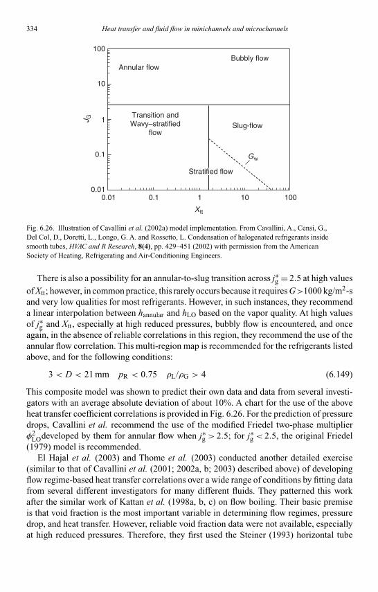
Kandlikar I044527-Ch06.tex 26/10/2005 18: 15 Page 334
334 Heat transfer and fluid flow in minichannels and microchannels
Annular flow
100
10
1
0.1
0.010.01 0.1 1 10 100
Bubbly flow
Transition andWavy–stratified
flowSlug-flow
Gw
Xtt
J G
Stratified flow
Fig. 6.26. Illustration of Cavallini et al. (2002a) model implementation. From Cavallini, A., Censi, G.,Del Col, D., Doretti, L., Longo, G. A. and Rossetto, L. Condensation of halogenated refrigerants insidesmooth tubes, HVAC and R Research, 8(4), pp. 429–451 (2002) with permission from the AmericanSociety of Heating, Refrigerating and Air-Conditioning Engineers.
There is also a possibility for an annular-to-slug transition across j∗g = 2.5 at high valuesof Xtt; however, in common practice, this rarely occurs because it requires G>1000 kg/m2-sand very low qualities for most refrigerants. However, in such instances, they recommenda linear interpolation between hannular and hLO based on the vapor quality. At high valuesof j∗g and Xtt , especially at high reduced pressures, bubbly flow is encountered, and onceagain, in the absence of reliable correlations in this region, they recommend the use of theannular flow correlation. This multi-region map is recommended for the refrigerants listedabove, and for the following conditions:
3 < D < 21 mm pR < 0.75 ρL/ρG > 4 (6.149)
This composite model was shown to predict their own data and data from several investi-gators with an average absolute deviation of about 10%. A chart for the use of the aboveheat transfer coefficient correlations is provided in Fig. 6.26. For the prediction of pressuredrops, Cavallini et al. recommend the use of the modified Friedel two-phase multiplierφ2
LOdeveloped by them for annular flow when j∗g > 2.5; for j∗g < 2.5, the original Friedel(1979) model is recommended.
El Hajal et al. (2003) and Thome et al. (2003) conducted another detailed exercise(similar to that of Cavallini et al. (2001; 2002a, b; 2003) described above) of developingflow regime-based heat transfer correlations over a wide range of conditions by fitting datafrom several different investigators for many different fluids. They patterned this workafter the similar work of Kattan et al. (1998a, b, c) on flow boiling. Their basic premiseis that void fraction is the most important variable in determining flow regimes, pressuredrop, and heat transfer. However, reliable void fraction data were not available, especiallyat high reduced pressures. Therefore, they first used the Steiner (1993) horizontal tube

Kandlikar I044527-Ch06.tex 26/10/2005 18: 15 Page 335
Chapter 6. Condensation in minichannels and microchannels 335
version of the Rouhani–Axelsson (1970) drift-flux void fraction map because it includesmass flux and surface tension effects:
α = x
ρV
([1 + 0.12(1 − x)]
[x
ρV+ 1 − x
ρL
]+ 1.18 (1 − x) [gσ (ρL − ρV)]0.25
Gρ0.5L
)−1
(6.150)
The void fraction predicted by this model does not approach the homogeneous void fractionas the critical pressure is approached. Therefore, they set about trying to improve upon thismodel by indirect means. They stated that turbulent annular flow condensation heat transferdata could in fact be used to deduce the applicable void fraction. This is because the corre-sponding liquid film heat transfer coefficient may be represented as h = c Ren
LPr0.5L (kL/δ),
where the film thickness δ is simply by definition δ= D(1 − α)/4. Substituting this expres-sion back into the heat transfer coefficient equation, it is clear that h ∝ (1 − x)n/(1 − α).Since void fractions in annular flow are very large, the denominator in this expression,representative of the liquid film thickness, is a small quantity that affects the heat transfercoefficient significantly. It is this sensitivity of the heat transfer coefficient to void fractionthat they sought to exploit in deducing the void fraction from available heat transfer data.Thus, they used the annular flow data from Cavallini et al. (2001; 2002a, b) to statisti-cally curve-fit the leading constant and exponent for ReL in the heat transfer expression,and assumed the Pr exponent to be 0.5 instead of 0.4. Although reasonable prediction wasachieved, the prediction accuracy seemed to show a strong saturation pressure dependency.Therefore, they decided, somewhat arbitrarily, that the actual void fraction would in fact liesomewhere between the Axelsson–Rouhani prediction and the homogeneous value. Theythen chose a logarithmic mean of these two values to represent the actual void fraction:
α = αhomogeneous − αAxelsson–Rouhani
ln(
αhomogeneous
αAxelsson–Rouhani
) (6.151)
This formulation was then used to curve-fit the heat transfer data again, which demonstratedan improvement in the prediction of the heat transfer data over a larger range of reducedpressures, which they took to be a validation of the void fraction curve-fit. Once thiswas established, they plotted the transitions between stratified, wavy, intermittent, annular,mist, and bubbly flow on G–x coordinates, adapting the transition expressions presented byKattan et al. (1998a, b, c) (with updates by Zurcher et al. (1999)) for boiling to the con-densing situation. For example, allowance is made for the fact that dryout does not occur incondensing flows; thus they remove that portion of the wavy transition line and arbitrarilyextend it from the minima of that transition to the x = 1 location. Various liquid–vaporcross-sectional areas and perimeters are derived from the void fraction to enable plotting ofthe transition lines. A representative map constructed in this manner is shown in Fig. 6.27. Itshould be noted that because the void fraction is dependent on the mass flux, strictly speak-ing, these maps have to be redrawn for each mass flux under consideration, even though Gis in fact one of the coordinates. However, El Hajal et al. state that the transition lines arenot very sensitive to the mass flux, and a first approximation may be achieved by choosing arepresentative mass flux to plot the transition lines. They demonstrate qualitative agreement
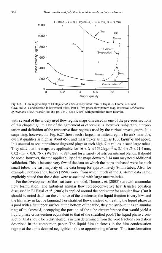
Kandlikar I044527-Ch06.tex 26/10/2005 18: 15 Page 336
336 Heat transfer and fluid flow in minichannels and microchannels
0 0.2
Mas
s ve
loci
ty (
kg/m
2 -s)
1200R-134a, G � 300 kg/m2-s, T � 40°C, d � 8 mm
1000
800
600
400
200
00.4 0.6 0.8
Vapor quality
CondensationSW
I A
GwavyXmin/wavy
Gstart
Gmist
Xmin/mist
q = 15 kW/m2
(Evaporation)
MF
XLA
1
Fig. 6.27. Flow regime map of El Hajal et al. (2003). Reprinted from El Hajal, J., Thome, J. R. andCavallini, A. Condensation in horizontal tubes, Part 1: Two-phase flow pattern map, International Journalof Heat and Mass Transfer, 46(18), pp. 3349–3363 (2003) with permission from Elsevier.
with several of the widely used flow regime maps discussed in one of the previous sectionsof this chapter. Quite a bit of the agreement or otherwise is, however, subject to interpre-tation and definition of the respective flow regimes used by the various investigators. It issurprising, however, that Fig. 6.27 shows such a large intermittent regime for an 8-mm tube,even at qualities as high as about 45% and mass fluxes as high as 1000 kg/m2-s and above.It is unusual to see intermittent slugs and plugs at such high G, x values in such large tubes.They state that the maps are applicable for 16<G< 1532 kg/m2-s, 3.14<D< 21.4 mm,0.02< pr < 0.8, 76< (We/Fr)L < 884, and for a variety of refrigerants and blends. It shouldbe noted, however, that the applicability of the maps down to 3.14 mm may need additionalvalidation. This is because very few of the data on which the maps are based were for suchsmall tubes, the vast majority of the data being for approximately 8-mm tubes. Also, forexample, Dobson and Chato’s (1998) work, from which much of the 3.14-mm data came,explicitly stated that these data were associated with large uncertainties.
For the development of the heat transfer model, Thome et al. (2003) start with an annularflow formulation. The turbulent annular flow forced-convective heat transfer equationdiscussed in El Hajal et al. (2003) is applied around the perimeter for annular flow. (But itshould be noted that near the entrance of the condenser, the liquid fraction is very low, andthe film may in fact be laminar.) For stratified flows, instead of treating the liquid phase asa pool with a flat upper surface at the bottom of the tube, they redistribute it as an annularring of thickness δ, occupying the portion of the tube circumference that would yield aliquid phase cross-section equivalent to that of the stratified pool. The liquid phase cross-section that should be redistributed is in turn determined from the void fraction correlationdescribed in the companion paper. The liquid film thickness in the film condensationregion at the top is deemed negligible in this re-apportioning of areas. This transformation

Kandlikar I044527-Ch06.tex 26/10/2005 18: 15 Page 337
Chapter 6. Condensation in minichannels and microchannels 337
allows them to use a gravity-driven Nusselt (1916) film condensation expression (with anassumption of zero vapor shear) in the upper part of the tube, coupled with the forced-convective annular flow expression for the lower portion of the circumference for whatwould otherwise be a liquid pool. The rest of the model is simply a weighted average ofthese different contributions based on the fraction of the circumference occupied by the“stratified” portion:
h = hfalling−filmrθ + hconvective(2π − θ)r
2πr(6.152)
Like most other models discussed in this section, all of the multiple regimes identified inthe first part of the study are handled either as (a) fully annular forced-convective, or as (b)consisting of varying combinations of upper gravity-driven, and lower forced-convectiveterms. It is stated that intermittent flow is very complex, and is therefore assumed to be pre-dicted by annular flow equations. Similarly, mist flow is handled as annular flow, assumingthat the liquid inventory entrained in the vapor phase can be viewed as an unsteady annularfilm. Bubbly flow is not modeled in this work, partly because it is not commonly encoun-tered. The novel manner of handling the stratified pool does, however, yield smoothertransitions between the heat transfer coefficient predictions across transitions. Further, thedegree of stratification is itself obtained through quadratic interpolation across the flowregime transition lines, ensuring a smooth introduction of the stratification component intothe heat transfer coefficient:
θ = θstrat
(Gwavy − G
Gwavy − Gstrat
)0.5
(6.153)
Another innovation introduced is the accounting of the effects of interfacial waves, usingconcepts of the “most dangerous” wavelength from stability considerations, and developingan enhancement factor due to interfacial roughness in terms of the slip ratio and theroughness amplitude:
fi = 1 +(
uV
uL
)j ((ρL − ρV) gδ2
σ
)k (G
Gstrat
)(6.154)
The exponents j and k are picked to be ½ and ¼ without discussion or substantiationfrom physical principles. The presence of the surface tension in the denominator correctlyimplies a decrease in the intensity (damping) of the interfacial waves at high surface tensionvalues. In addition, the last term in the equation ensures that the waves are progressivelydamped out upon approach to fully stratified conditions, although why this term should bea linear decrease (evidenced by the exponent of 1 for this term) and not raised to anotherexponent is not made clear. The authors present numerous graphs to demonstrate thatthe predictions are not biased toward underprediction or overprediction with respect tothe independent variables. Their model predicts the data from the large database over awide range of fluids, operating conditions, and diameters (with the caution stated aboveabout the applicability to the 3.14-mm diameter) well, with 85% of the refrigerant heattransfer data predicted within 20%. It is interesting to note that this is about the same

Kandlikar I044527-Ch06.tex 26/10/2005 18: 15 Page 338
338 Heat transfer and fluid flow in minichannels and microchannels
0 0.2
14,000
12,000
10,000
8000
6000
4000
2000
0.4 0.6Vapor quality
SW
MF
A
S
A
A
R-410A, d � 8 mm, Tsat � 40°C, q � 40 kW/m2H
eat t
rans
fer
coef
ficie
nt (
W/m
2k)
0.8 1
G � 30 kg/m2sG � 200 kg/m2sG � 500 kg/m2sG � 800 kg/m2s
Fig. 6.28. Heat transfer coefficient trends predicted by the Thome et al. (2003) model. Reprinted from Thome,J. R., El Hajal, J. and Cavallini, A., Condensation in horizontal tubes, Part 2: New heat transfer model based onflow regimes, International Journal of Heat and Mass Transfer, 46(18), pp. 3365–3387 (2003) with permissionfrom Elsevier.
level of predictive accuracy as the earlier multi-flow regime correlations proposed byCavallini et al. (2002a). This model does offer some new approaches – heat transferdata are used to refine a void fraction model, which is then used to predict flow regimetransitions, which are in turn used to predict a “tuned blend” of stratified-convective heattransfer coefficients. It achieves smoothly varying heat transfer coefficients across multipleregimes (Fig. 6.28) with good accuracy, using some first principles concepts and severalkey assumptions and empirical constants or curve-fitted terms at appropriate locations forclosure. Additional substantiation of the use of an average of homogeneous and Steiner(1993)/Rouhani–Axelsson (1970) void fractions, and the physical basis for extensions oftransition lines determined from boiling considerations would lend further credence to themodel. Measurement, rather than deduction from heat transfer data, of the fundamentalunderlying quantity (void fraction), to which the authors credit much of the success of thisapproach, would also enhance its predictive abilities. This would be particularly importantif the model were to be extended in the future to microchannels.
Goto et al. (2003) measured heat transfer coefficients for the condensation of R-410Aand R-22 inside five different helical and herringbone internally grooved tubes of about8.00-mm OD. Local heat transfer coefficients were measured for 130<G< 400 kg/m2-sand Tsat = 30◦C and 40◦C by dividing a 1-m long test section into 10 small sections.Unlike most other studies discussed in this chapter, the heat transfer tests were conductedin a complete vapor compression system. The reported uncertainties in the heat transfercoefficients were very high, about 40%. Heat transfer coefficients of the herringbonegrooved tube were found to be about twice as large as those for the helical grooved tubes.Using Koyama and Yu’s (1996) Nu = (Nu2
annular + Nu2stratified)0.5 correlation for stratified
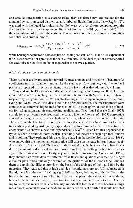
Kandlikar I044527-Ch06.tex 26/10/2005 18: 15 Page 339
Chapter 6. Condensation in minichannels and microchannels 339
and annular condensation as a starting point, they developed new expressions for theannular flow portion based on their data. A turbulent liquid film basis, Nu = Re∗
LPrL/T ∗i ,
was used, with the liquid Reynolds number Re∗L = (ρL
√τw/ρL D)/µL computed from the
friction velocity with the two-phase multiplier of Goto et al. (2001) φv = 1 + 1.64X 0.79tt for
the computation of the wall shear stress. This approach resulted in following correlationfor helical and cross microfins:
Nuannular = 0.743√
f
(φv
Xtt
)(µL
µV
)0.1 ( x
1 − x
)0.1
Re0.7L (6.155)
while herringbone microfin tubes required a leading constant of 2.34, and a Re exponent of0.62. These correlations predicted the data within 20%. Individual equations were reportedfor each tube for the friction factor required in the above equation.
6.5.2. Condensation in small channels
There has been a slow progression toward the measurement and modeling of heat transfercoefficients in small channels, and unlike the studies on flow regimes, void fraction andpressure drop cited in previous sections, there are few studies that address Dh ≤ 1 mm.
Yang and Webb (1996a) measured heat transfer in single- and two-phase flow of refrig-erant R-12 at 65◦C in rectangular plain and microfin tubes with Dh = 2.64 and 1.56 mm,respectively, using the modified Wilson plot technique. The companion pressure drop study(Yang and Webb, 1996b) was discussed in the previous section. The measurements wereconducted at somewhat higher mass fluxes (400<G< 1400 kg/m2-s) than those of inter-est for refrigeration and air-conditioning applications. They found that the Shah (1979)correlation significantly overpredicted the data, while the Akers et al. (1959) correlationshowed better agreement, except at high mass fluxes, where it also overpredicted the data.The microfin tube heat transfer coefficients showed steeper slopes than those for the plaintubes when plotted against quality, especially at the lower mass fluxes. The heat transfercoefficients also showed a heat flux dependence (h ∝ q′′0.2); such heat flux dependence istypically seen in stratified flows (which is certainly not the case at such high mass fluxes)and in boiling. They explained this dependence based on the work of Soliman et al. (1968),who argued that the momentum contribution will cause an increase in heat transfer coef-ficient when q′′ is increased. Their results also showed that the heat transfer enhancementdue to the microfins decreased with increasing mass flux. By plotting the heat transfer dataagainst the equivalent mass velocity Reynolds number proposed by Akers et al. (1959),they showed that while data for different mass fluxes and qualities collapsed to a singlecurve for plain tubes, this only occurred at low qualities for the microfin tube. This ledthem to explain the different trends on the basis of the drainage of the liquid film by themicrofins. They reasoned that at high qualities, the microfins are not fully submerged inliquid; therefore, they act like Gregorig (1962) surfaces, helping to drain the film to thebase of the fins, thus increasing heat transfer over the plain tube values. At low qualities,however, the fins are submerged; therefore, the drainage mechanism is not active. Accord-ing to them, this mechanism is particularly important at low mass fluxes, because at highmass fluxes, vapor shear exerts the dominant influence on heat transfer. It should be noted

Kandlikar I044527-Ch06.tex 26/10/2005 18: 15 Page 340
340 Heat transfer and fluid flow in minichannels and microchannels
that in the companion work, Yang and Webb (1996b) had concluded that surface tensiondid not play a role in determining the pressure drop in these same tubes.
Yang and Webb (1997) continued this work to develop a heat transfer model for con-densation of R-12 and R-134a in extruded microchannels (Dh = 1.41 and 1.56 mm) withmicrofins (0.2- and 0.3-mm deep). The data for these channels were reported in their earlierpapers cited above. They used the observations discussed above about the contribution ofvapor shear and surface tension to represent the heat transfer coefficient as follows:
h = huAu
A+ hf
Af
A(6.156)
where the subscripts u and f refer to unflooded and flooded portions of the channel, respec-tively. They calculated the surface and cross-sectional areas of the liquid in the drainageregions using the geometric features of the microfin, and the Zivi (1964) void fraction modelto estimate the liquid volume occupying the drainage region. For flooded conditions (e.g.at low vapor qualities) they used a slightly modified version of the Akers et al. (1959)model (which corresponds to their experimentally derived single-phase Nusselt numberNuDh = 0.10Re0.73
DhPr1/3
l ) to compute the shear-driven heat transfer coefficient. When themicrofins were unflooded, they assumed a thin laminar film draining on the walls of themicrofin and computed the pressure gradients in the axial and microfin wall directionsdue to vapor shear and surface tension, respectively. These perpendicular vapor shear (sh)and surface tension (st) stresses were combined to yield the wall shear stress, which wasthen related to the unflooded heat transfer coefficient, h2
u = h2sh + h2
st. Relating the surface-tension-driving force to the microfin profile and the Weber number We = (G2
eqDh)/(ρlσ),they developed the following expression for the surface tension contribution to the heattransfer coefficient:
hst = Cτz − τi
dp/dzkl
d (1/r)
ds
ReeqPrl1/3
We(6.157)
where z refers to the axial direction, subscript i refers to the interface, and C was derivedthrough regression of their data to be 0.0703. The relative fractions of the surface tensionand vapor shear contributions to the heat transfer coefficient were plotted to show that at lowmass flux (G = 400 kg/m2-s) and x> 0.5, the surface tension contribution could equal andexceed the vapor shear term. At high mass fluxes (G = 1400 kg/m2-s), the surface tensioncontribution was very small. A small fin tip radius enhanced the heat transfer, while a largeinter-fin drainage area allowed the surface tension effect to be activated at lower qualities.
Kim et al. (2003) conducted a study similar to that of Yang and Webb (1996a, b; 1997)above, on similar tubes (Dh = 1.41 smooth, 1.56-mm microfin with 39% greater surfacearea than the smooth tube), with a similar experimental set up using R-22 and R-410A for200<G< 600 kg/m2-s at 45◦C. Representative tube cross-sections and the test sectionused for the experiments is shown in Fig. 6.29. To test the tubes, they formed a jacketaround the channel with a 1-mm gap. Since the Wilson plot technique was used, it wasimportant to minimize the coolant-side resistance (an issue not recognized or stated byinvestigators often enough.) In their tests, the coolant side constituted approximately 1/3of total resistance. Further decreases could not be achieved because the required highercoolant flow rates would result in an extremely small coolant temperature rise, which
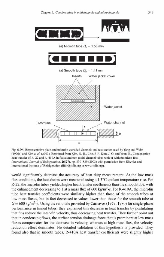
Kandlikar I044527-Ch06.tex 26/10/2005 18: 15 Page 341
Chapter 6. Condensation in minichannels and microchannels 341
(a) Microfin tube Dh � 1.56 mm
P
ero g
rb
(a) Smooth tube Dh � 1.41 mm
Inserts Water jacket cover
Water jacket
Water channelTest tube
w
t
b
Fig. 6.29. Representative plain and microfin extruded channels and test section used by Yang and Webb(1996a) and Kim et al. (2003). Reprinted from Kim, N.-H., Cho, J.-P., Kim, J.-O. and Youn, B., Condensationheat transfer of R–22 and R–410A in flat aluminum multi-channel tubes with or without micro-fins,International Journal of Refrigeration, 26(27), pp. 830–839 (2003) with permission from Elsevier andInternational Institute of Refrigeration ([email protected] or www.iifiir.org).
would significantly decrease the accuracy of heat duty measurement. At the low massflux conditions, the heat duties were measured using a 1.3◦C coolant temperature rise. ForR-22, the microfin tubes yielded higher heat transfer coefficients than the smooth tube, withthe enhancement decreasing to 1 at a mass flux of 600 kg/m2-s. For R-410A, the microfintube heat transfer coefficients were similarly higher than those of the smooth tubes atlow mass fluxes, but in fact decreased to values lower than those for the smooth tube atG = 600 kg/m2-s. Using the rationale provided by Carnavos (1979; 1980) for single-phaseperformance in finned tubes, they explained this decrease in heat transfer by postulatingthat fins reduce the inter-fin velocity, thus decreasing heat transfer. They further point outthat in condensing flows, the surface tension drainage force that is prominent at low massfluxes compensates for the decrease in velocity, whereas at high mass flux, the velocityreduction effect dominates. No detailed validation of this hypothesis is provided. Theyfound also that in smooth tubes, R-410A heat transfer coefficients were slightly higher

Kandlikar I044527-Ch06.tex 26/10/2005 18: 15 Page 342
342 Heat transfer and fluid flow in minichannels and microchannels
than those of R-22, while the opposite was true for microfin tubes. In smooth tubes, thehigher R-410A heat transfer coefficients were attributed to its larger thermal conductivityand smaller viscosity. In microfin tubes, however, they noted that theWeber number of R-22was 2.7 times lower than that of R-410A at the test conditions, leading to greater surfacetension drainage and heat transfer. The two times larger vapor-to-liquid volume ratio ofR-22 was also believed to have resulted in a larger fraction of the fin surface being exposedto the vapor, thus enhancing heat transfer. Several other plausible explanations in termsof the fluid properties are provided, although additional validation would be necessary toconfirm these explanations of the small differences in heat transfer coefficients, especiallyin view of the uncertainties in the measurement of heat transfer coefficients at these smallheat transfer rates. Based on these trends, they recommended the use of Moser et al.’s(1998) model with a modified two-phase multiplier for the smooth tubes, and Yang andWebb’s (1997) model with minor modifications for the microfin tubes.
Yan and Lin (1999) measured heat transfer coefficients during condensation of R-134athrough a bank of 2-mm tubes arranged in parallel. Their pressure drop results were dis-cussed in the previous section. Copper plates, 5-mm thick, were soldered on to the bank ofrefrigerant tubes, and coolant tubes were in turn soldered on to the copper plates to providea crossflow cooling orientation. The authors state that the tubes and the plate had goodthermal contact, eliminating the need for avoiding gaps between the tubes and the plates.However, they provide no substantiation that the thermal resistance from the refrigerant tothe coolant through the refrigerant and coolant tubes, the gaps between the plates and thetubes, and the two 5-mm thick copper plates was either accounted for properly, or was in factsmall in magnitude. The issue of mal-distribution through the 28 parallel channels was alsonot discussed in detail, except to state that the inlet and outlet headers were appropriatelydesigned. Their single-phase friction factors were significantly higher than the predictionsof the Blasius equation, and the single-phase heat transfer coefficients were also higherthan the predictions of the Gnielinski (1976) correlations. Entrance length effects and tuberoughness may have accounted for some of this, according to the authors. Condensationheat transfer coefficients were higher at the lower saturation temperatures, especially atthe higher qualities. They attributed this to the lower thermal conductivity of R-134a at thehigher temperatures. The heat transfer coefficients also decreased significantly as the heatflux was increased, particularly at the higher qualities. This is not typical of condensationheat transfer, where any heat flux (orT ) dependence is usually seen at the lower qualitiesin gravity-dominated flow. The graphs they presented to demonstrate the effect of mass fluxshow inflection points where the heat transfer coefficient first increased sharply as qualityis increased from around 10–20%, followed by a flattening with further increases in qualityat the lower mass fluxes, finally again increasing with quality. Adequate explanations forthese trends are not provided. They proposed the following correlation for their data:
hD
klPr−0.33
l Bo0.3 Re = 6.48Re1.04eq Bo = q′′
hfgG(6.158)
It is not clear why the Reynolds number as well as the equivalent Reynolds numberaccording to the Akers et al. (1959) model were required to correlate the data.

Kandlikar I044527-Ch06.tex 26/10/2005 18: 15 Page 343
Chapter 6. Condensation in minichannels and microchannels 343
Rectangular channels with Dh = 1.46 mm (1.50 × 1.40 mm) were investigated by Wanget al. (2002) for the condensation of R-134a at 61.5–66◦C over the mass flux range75–750 kg/m2-s. The experiments were conducted in 610-mm long tubes with finned 10multi-port channels cooled by air in crossflow. Flow visualization experiments were alsoconducted by replacing one aluminum wall of the tube with a glass window to help deter-mine the applicable flow regimes. The authors report inlet qualities to the test section,which were controlled over a wide range; however, the quality change across the test sec-tion was substantial, indicating that for many of the tests, the experiments did not yieldlocal heat transfer coefficients over small increments of quality. From the combinationof flow visualization and heat transfer experiments, they note that even in a channel thissmall, stratified (wavy) flows were seen at the low mass fluxes. The heat transfer coef-ficients were insensitive to quality at the low mass fluxes. At the high mass fluxes, thedependence on quality was strong, signifying annular flow. Of the available heat transfercorrelations, the Akers et al. (1959) equivalent Re correlation was found to agree mostwith their data in the annular flow regime, while the Jaster and Kosky (1976) correlationagreed best with their stratified flow data. However, they noted that the Reeq concept ofAkers et al. (1959) does not explicitly account for the applicable flow regime, because Reeqcan be the same for different flow regimes. They attempted to improve the predictions bydeveloping their own stratified and annular flow correlations. They separated the data intostratified and annular regimes using the Breber et al. (1980) and Soliman (1982; 1986)transition criteria. Their stratified–annular transition occurred at a lower gas superficialvelocity ( j∗g = 0.24 m/s) than that predicted by the Breber et al. map, because the cornersof the rectangular channel aided the formation of annular flow. This earlier transition toannular flows was also observed with respect to the Soliman map, while the annular–misttransition was not observed. For annular flow, they conducted a boundary-layer analysissimilar to Traviss et al. (1973), and through the analysis of their data, proposed the fol-lowing curve-fits for the two-phase multiplier, and unlike most other researchers, for thedimensionless temperature as well:
φv =√
1.376 + 8X 1.655tt T+
δ = 5.4269(
Rel
x
)0.2208
(6.159)
The resulting annular flow correlation was as follows:
Nuannular = 0.0274 Prl Rel0.6792x0.2208
(1.376 + 8X 1.655
tt
X 2tt
)0.5
(6.160)
For stratified flows, they used the Chato (1962) correlation for the film condensationportion, and the Dittus–Boelter (1930) correlation for forced convection in the liquid pool,combining the two as follows:
Nustratified = αNufilm + (1 − α)Nuconvection (6.161)
Therefore, they essentially used the Zivi (1964) void fraction as a measure of the liq-uid pool height in this rectangular channel. In addition, for design purposes, especially

Kandlikar I044527-Ch06.tex 26/10/2005 18: 15 Page 344
344 Heat transfer and fluid flow in minichannels and microchannels
since their condensation tests were conducted over large quality changes, they proposeda weighted average between these two correlations using the quality at Soliman Froudenumber Frso = 8 as the transition between the regimes.
Koyama et al. (2003b) conducted a study on the condensation of R-134a in twomulti-port extruded aluminum tubes with eight 1.11-mm channels, and nineteen 0.80-mmchannels, respectively. Local heat transfer coefficients were measured at every 75 mm ofthe 600-mm long cooling section using heat flux sensors. They acknowledged that it is verydifficult to accurately measure local heat transfer coefficients in such small channels usingthe temperature rise in the coolant or a Wilson plot method due to the inaccuracies asso-ciated with the measurement of low heat transfer rates and small temperature differences.The tests were conducted over the range 100<G< 700 kg/m2-s at 60◦C. For correlat-ing their data, they used a combination of convective and film condensation terms to yieldNu = (Nu2
annular + Nu2stratified)0.5. The individual annular and stratified terms were obtained
from the work of Haraguchi et al. (1994a, b), except that their two phase multiplier wasreplaced by the multiplier proposed by Mishima and Hibiki (1996). They stated that thiswas an improvement over several other correlations; however, the graphs of predicted andexperimental Nusselt numbers show consistent and large (as high as 80%) overpredictionsof all their data at almost all conditions.
In some recent studies, Wang, Rose, and co-workers have developed analyticalapproaches for addressing condensation heat transfer in triangular (Wang and Rose, 2004)and square (Wang et al., 2004; Wang and Rose, 2005) microchannels. For film condensa-tion of R-134a in horizontal 1-mm triangular channels, Wang and Rose (2004) assumedthat the condensate was in laminar flow, and developed one of the first models that accountsfor surface tension, shear stress, and gravity. They were able to predict and substantiate thevarying condensate flow pattern across the cross-section as well as along the length of thechannel. Thus, they were able to model the corresponding variations in heat transfer coeffi-cient. Using a similar approach, Wang et al. (2004) developed a model for film condensationof R-134a in square, horizontal, 1-mm microchannels. As these papers account for the threeprimary governing influences in microchannel condensation, they provide a good start forthe modeling of phenomena specific to microchannels. Furthermore, the respective forcescan be “switched on or off” to understand their respective significances (Fig. 6.30).
In another recent study, Cavallini et al. (2005) conducted measurements of heat transfercoefficients and pressure drops during condensation of R-134a and R-410A inside multipleparallel 1.4-mm Dh channels. The test section was divided into three separate segmentsto provide quasi-local pressure drops and heat transfer coefficients. They deduced thefrictional pressure drop from the measured drop in saturation temperature and found goodagreement between the data for R-134a and the correlations of Friedel (1979), Zhang andWebb (2001), Mishima and Hibiki (1996), and Mueller-Steinhagen and Heck (1986). All ofthese correlations were found to overpredict the R-410A data, however. Their heat transfercoefficients were obtained from wall temperature measurements, and they found that theavailable models in the literature (Akers et al., 1959; Moser et al., 1998; Zhang and Webb,2001; Cavallini et al., 2002a; Wang et al., 2002; Koyama et al., 2003a) underestimatedtheir results, particularly at high values of mass flux. They attributed these differences tothe much higher gas velocities in their experiments where mist flow might prevail, whereasthe available correlations are primarily for annular flow in larger diameter tubes.

Kandlikar I044527-Ch06.tex 26/10/2005 18: 15 Page 345
Chapter 6. Condensation in minichannels and microchannels 345
0 100 200 300 400 500 6000
5
10
15
z (mm)
b � 1.0 mm Ts � 50°C�T � 6 K G � 500 kg/m2-s
R-134a
g � 0
az
(kW
/m2-
K)
t, s, g all included
s � 0, g � 0
Fig. 6.30. Variation of mean heat transfer coefficient along a square 1-mm channel. Reprinted fromWang, H. S. and Rose, J. W., A theory of condensation in horizontal non-circular microchannels,ASME Journal of Heat Transfer, in press (2005).
Shin and Kim (2005) used a technique that matched the outlet temperature of an elec-trically heated air stream with that of a similar air stream heated by condensing refrigerantR-134a to measure small, local condensation heat transfer rates. Circular and square chan-nels with 0.5<Dh < 1 mm were tested for the mass flux range 100<G< 600 kg/m2-s at40◦C. For circular and square channels, they also found that most of the available modelsand correlations discussed above (Akers et al., 1959; Soliman et al., 1968; Traviss et al.,1973; Cavallini and Zecchin, 1974; Shah, 1979; Dobson, 1994; Moser et al., 1998) under-predict their data at the low mass fluxes, which they deemed to be the important range forengineering applications. The agreement with these correlations improved somewhat at thehigher mass fluxes. Although they found no significant effect of the heat flux, they notedthat at lower mass fluxes, square channels had higher heat transfer coefficients than thosefor circular channels, whereas the reverse was true for high mass fluxes. No satisfactoryexplanation was provided for these trends.
Garimella and Bandhauer (2001) conducted heat transfer experiments using the tubes(0.4<Dh < 4.9 mm) that were used for the pressure drop experiments of Garimella et al.(2002; 2003a, b; 2005) described above. They specifically addressed the problems in heattransfer coefficient determination due to the high heat transfer coefficients and low massflow rates in microchannels. For the small x required for local measurements, the heatduties at the mass fluxes of interest are relatively small, and to ensure reasonable accu-racies in heat duty measurement, the coolant inlet-to-outlet temperature difference mustbe increased to minimize uncertainties. However, since this requires low coolant flowrates, the coolant-side thermal resistance becomes dominant, making it difficult to deducethe refrigerant-side resistance from the measured UA. These conflicting requirements forthe accurate measurement of heat duty and the refrigerant heat transfer coefficients wereresolved by developing a thermal amplification technique (Fig. 6.31) that decoupled thesetwo issues. Thus, the test section was cooled using water flowing in a closed (primary) loopat a high flow rate to ensure that the condensation side presented the governing thermal
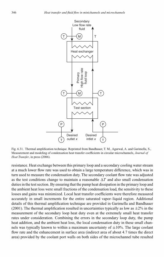
Kandlikar I044527-Ch06.tex 26/10/2005 18: 15 Page 346
346 Heat transfer and fluid flow in minichannels and microchannels
SecondaryLow flow rate
fluid
Prim
ary
Hig
h flo
w r
ate
fluid
loop
Heat exchanger
Test section
P
T
Desiredoutlet x
Desiredintlet x
P
T
T M T
T TM
Fig. 6.31. Thermal amplification technique. Reprinted from Bandhauer, T. M., Agarwal, A. and Garimella, S.,Measurement and modeling of condensation heat transfer coefficients in circular microchannels, Journal ofHeat Transfer, in press (2006).
resistance. Heat exchange between this primary loop and a secondary cooling water streamat a much lower flow rate was used to obtain a large temperature difference, which was inturn used to measure the condensation duty. The secondary coolant flow rate was adjustedas the test conditions change to maintain a reasonable T and also small condensationduties in the test section. By ensuring that the pump heat dissipation in the primary loop andthe ambient heat loss were small fractions of the condensation load, the sensitivity to theselosses and gains was minimized. Local heat transfer coefficients were therefore measuredaccurately in small increments for the entire saturated vapor–liquid region. Additionaldetails of this thermal amplification technique are provided in Garimella and Bandhauer(2001). The thermal amplification resulted in uncertainties typically as low as ±2% in themeasurement of the secondary loop heat duty even at the extremely small heat transferrates under consideration. Combining the errors in the secondary loop duty, the pumpheat addition, and the ambient heat loss, the local condensation duty in these small chan-nels was typically known to within a maximum uncertainty of ±10%. The large coolantflow rate and the enhancement in surface area (indirect area of about 4.7 times the directarea) provided by the coolant port walls on both sides of the microchannel tube resulted

Kandlikar I044527-Ch06.tex 26/10/2005 18: 15 Page 347
Chapter 6. Condensation in minichannels and microchannels 347
14,000
12,000
10,000
8000
6000
4000
2000
00.1 0.2 0.3 0.4 0.5 0.6
Quality (x)
Hea
t tra
nsfe
r co
effic
ient
(W
/m2 -
K)
0.7 0.8 0.9
G � 150 kg/m2-sG � 300 kg/m2-sG � 450 kg/m2-sG � 600 kg/m2-sG � 750 kg/m2-s
D � 0.506 mmD � 0.761 mmD � 1.520 mm
Fig. 6.32. Microchannel condensation heat transfer coefficients. From Bandhauer, T. M., Agarwal, A. andGarimella, S., Measurement and modeling of condensation heat transfer coefficients in circular microchannels,Journal of Heat Transfer, in press (2006).
in high refrigerant-to-coolant resistance ratios (between 5 and 30). With this high resis-tance ratio, even an uncertainty of ±25% in the tube-side heat transfer coefficient did notappreciably affect the refrigerant-side heat transfer coefficient, ensuring low uncertainties.Representative heat transfer coefficients reported by Bandhauer et al. (2005) are shown inFig. 6.32. In general, the heat transfer coefficient increases with decreasing diameter, withthe effect of diameter becoming more significant at the higher qualities (∼x> 0.45) andmass fluxes. Thus, h increases between 10% and 40% for x> 0.45 as Dh is reduced from1.524 to 0.506 mm, with the effect of Dh being more significant for a decrease in Dh from0.761 to 0.506 mm. Gravity-driven correlations were found to be poor predictors of thedata, with the Chato (1962) correlation underpredicting the data considerably, the Jasterand Kosky (1976) correlation resulting in significant overprediction, and the Rosson andMyers (1965) and Dobson and Chato (1998) correlations being somewhat better – theselatter correlations account for heat transfer through the bottom of the tube. This is notsurprising because these models are not appropriate for Garimella and Bandhauer’s data,which were demonstrated to be not in the stratified wavy regimes (Coleman and Garimella,2000a; 2003). Among correlations that use a two-phase multiplier approach, the Moseret al. correlation predicted the data reasonably well (14% average deviation), with theShah (1979) and Cavallini and Zecchin (1974) correlations resulting in some overpredic-tion. Homogeneous flow correlations of Boyko and Kruzhilin (1967) and the mist flowcorrelation of Soliman (1986) were better at predicting the data, with the Soliman corre-lation leading to some overprediction. Shear-dominated annular flow correlations usingboundary-layer treatments also showed reasonable agreement: Soliman et al. (1968) (18%average deviation), Chen and Kocamustafaogullari (1987) (13% average deviation.) How-ever, in spite of the theoretical basis of the Traviss et al. (Traviss and Rohsenow, 1973;Traviss et al., 1973) correlation, as reported by several investigators, this model showedthe largest average deviation (38%) among shear-driven treatments.

Kandlikar I044527-Ch06.tex 26/10/2005 18: 15 Page 348
348 Heat transfer and fluid flow in minichannels and microchannels
Bandhauer et al. (2005) noted that during the condensation process, the flow changesfrom mist flow (where applicable) to annular film flow to intermittent, with large overlapsin the types of flow resulting in transition flow (intermittent/annular, intermittent/annular/mist, and annular/mist). Based on the work of Coleman and Garimella (2000a; 2003), wavyflow was not expected in any of the channels considered. Due to the large overlap regionsbetween these flows, with the bulk of the data being in transition between annular flow andother regimes, they developed a heat transfer model based on annular flow considerations.They noted that many of the available shear-driven models, though sound in formulation,led to poor predictions because of the inadequate calculation of shear stresses using pressuredrop models that were not applicable to microchannels. Thus, their model is based onboundary-layer analyses, but with the requisite shear stress being calculated from thepressure drop models of Garimella et al. (2005) developed specifically for microchannels.Since in annular flow, the condensate layer might become turbulent at very low Rel (∼240)(Carpenter and Colburn, 1951) due to the turbulent vapor core and the destabilizing effectof condensation (Schlichting and Gersten, 2000), a model based on turbulent parameterswith appropriate modifications for the conditions under study was developed. The frictionvelocity u∗ = √
τi/ρl was expressed in terms of the interfacial shear stress, rather than thecommonly used wall shear stress. The turbulent dimensionless temperature was defined asfollows:
T+ = ρl × Cpl × u∗
q′′ (Ti − Tw) (6.162)
The shear stress and heat flux were expressed in the usual manner:
τ = (µ+ ρ × εm)du
dy(6.163)
q′′ = −(k + εh × ρ × Cp)dT
dy(6.164)
Assuming that the all of the heat is transferred in the liquid film results in the follow-ing expression for the heat transfer coefficient, where the interface is at the saturationtemperature:
h = q′′
(Tsat − Tw)= ρl × Cpl × u∗
T+ (6.165)
The heat flux above yields the dimensionless temperature gradient:
dT+
dy+ =(
1
Prl+ ρl × εh
µl
)−1
(6.166)
To integrate this, the turbulent film thickness δ= (1 − √α)D/2 is determined using the
Baroczy (1965) model, which is different from the manner in which Traviss et al. (Travissand Rohsenow, 1973; Traviss et al., 1973) determined film thickness. The dimensionless

Kandlikar I044527-Ch06.tex 26/10/2005 18: 15 Page 349
Chapter 6. Condensation in minichannels and microchannels 349
turbulent film thickness is then δ+ = (δρlu∗)/µl. Also τ= (1 − y/R)τw yields the followingequation:
ρlεm
µl= 1 − y+/R+
du+/dy+ − 1 (6.167)
In a manner analogous to the development by Traviss et al. (1973), with the assumptionsof small film thickness compared to the tube radius, and εm ∼= εh, the following simplifiedtwo-region turbulent dimensionless temperature expressions were proposed:for Rel < 2100:
T+ = 5Prl + 5 ln[
Prl
(δ+
5− 1
)+ 1
](6.168)
for Rel > 2100:
T+ = 5Prl + 5 ln(5Prl + 1)+∫ δ+
30
dy+(1
Prl− 1
)+ y+
5
(1 − y+
R+) (6.169)
The only unknown quantity, the interfacial shear stress for determining u∗, is obtained fromthe annular flow portion of the multiple-flow regime pressure drop model by Garimellaet al. (2005) discussed in the previous section. Thus, the interfacial friction factor (and thenthe interfacial shear stress) is computed from the corresponding liquid-phase Re and fric-tion factor, the Martinelli parameter, and the surface tension parameter: fi/fl = AX a Reb
l ψc.
Additional details are available in the previous section. In summary, to obtain the heat trans-fer coefficient, the interfacial shear stress is first calculated using the pressure drop model.The resulting shear stress is used to compute the friction velocity u∗ and the dimensionlessfilm thickness δ+. The dimensionless temperature T+ is then calculated, which yields theheat transfer coefficient. This model predicted 86% of the data within ±20%, with anaverage absolute deviation of 10%. A more explicit accounting of the heat transfer in theliquid slugs, vapor bubbles, and the film-bubble interface in intermittent flow, and of theentrainment of liquid into the vapor core in mist flow would improve the predictions further.The data and the predictions at representative mass fluxes for each tube are shown in Fig.6.33. The heat transfer coefficient increases with an increase in mass flux and quality, andwith a decrease in the tube diameter. As the liquid film becomes thinner with increasingvapor quality, the heat transfer coefficient increases. The steep slope at the higher qualitiesrepresents an approach to a vanishingly thin film. However, it must be noted that the actualbehavior in this region will be dependent on the inlet conditions of a condenser, includingthe inlet superheat, the coolant temperature, and the consequent wall subcooling – thesephenomena are not accounted for in this model. Although the model was developed basedon an annular flow mechanism, it appears to predict the heat transfer coefficients in themist and mist–annular overlap regions in the high mass flux and high-quality cases ade-quately. At the extreme end of the graph (x> 80%), the flow may be exclusively in the mistflow region. For a given flow rate, the quality at which the mist flow regime occurs could

Kandlikar I044527-Ch06.tex 26/10/2005 18: 15 Page 350
350 Heat transfer and fluid flow in minichannels and microchannels
Pre
dict
ed a
nd e
xper
imen
tal h
(W
/m2 -
K)
G � 750 kg/m2-s
00.0 0.2 0.4 0.6
Quality (x)
0.8 1.0
14,000
12,000
10,000
8000
6000
4000
2000
G � 600 kg/m2-s
0
14,000
12,000
10,000
8000
6000
4000
2000
14,000G � 450 kg/m2-s
12,000
10,000
8000
6000
4000
2000
0
Data model0.506 mm0.761 mm1.524 mm
Fig. 6.33. Microchannel condensation heat transfer coefficient predictions. From Bandhauer, T. M.,Agarwal, A. and Garimella, S., Measurement and modeling of condensation heat transfer coefficients incircular microchannels, Journal of Heat Transfer, in press (2006).
decrease with decreasing diameter due to increased interfacial shedding. As liquid entrain-ment increases, the heat transfer coefficient will increase due to the thinning of the liquidfilm (Soliman, 1986). Although liquid entrainment and mist formation are not explicitlyaccounted for in the heat transfer part of this model, the trends in the data (the steeper slopein the data at the higher qualities, particularly for small Dh) can be interpreted on this basis.

Kandlikar I044527-Ch06.tex 26/10/2005 18: 15 Page 351
Chapter 6. Condensation in minichannels and microchannels 351
6.5.3. Summary observations and recommendations
The above discussion of the available literature on condensation heat transfer shows thatmuch of the available information is on tubes larger than about 7 mm. In these tubes, heattransfer models have treated the multitude of flow regimes identified by many investiga-tors and discussed in the previous sections as either stratified or annular flow regimes.Thus, almost all the available models in essence still use only gravity- or shear-dominatedapproaches. What differs from investigator to investigator is the specific analysis thataddresses these two modes. In models of gravity-dominated condensation for example,the earliest models were patterned very closely after the Nusselt condensation analysis.They then progressed from neglecting the heat transfer in the liquid pool to accounting forit in some manner, usually through the application of single-phase liquid forced-convectiveheat transfer correlations. The apportioning of film condensation and forced convectionregions within this stratified flow has also differed in the minor details. Most of these mod-els use some void fraction model, usually the one by Zivi (1964), to determine the liquidand vapor fractions of the cross-section (which is usually quantified as the liquid poolangle), which then allows them to predict the surface area over which these two submodelsare applied. In many cases, however, the void fraction models were originally based onannular flow data or analyses. A few models have also attempted to account for vapor shearon the falling-film condensation portion of the tube.
In annular flow models, the technique of relating the interfacial shear (through aboundary-layer analysis that usually uses the von Karman velocity profile) to the heattransfer across the liquid film has been used widely, starting with the work of Carpenterand Colburn (1951), with refinements and improvements to the contribution of variousforces to the interfacial shear, for example by Soliman (1968), Traviss et al. (1973), andothers. There have also been some attempts such as the work of Chen et al. (1987) todevelop general purpose annular flow correlations starting with asymptotic limits, andblending them through some simple combination of the terms at the respective limits.Another approach has been to directly apply a multiplication factor to a single-phaseliquid or vapor phase heat transfer correlation, with the multiplier determined using adap-tations of the Lockhart–Martinelli (1949) and Friedel (1979) pressure drop multipliers.This approach is in fact analogous to the boundary-layer shear stress analysis used bymany investigators. The only essential difference is in where the multiplier is applied: thefirst type of models use the multiplier first for shear stress determination, and calculatethe heat transfer coefficient directly thereafter; the second type calculate the single-phaseheat transfer coefficient directly, and apply the multiplier thereafter. An explanation of thesimilarity of these two approaches is provided in Dobson and Chato (1998). One correla-tion that continues to be used frequently is the purely empirical Shah (1979) correlation,because of its simplicity, the wide range of data that were utilized in its development, andits comparatively good predictions for annular flows. Another model that has been usedwidely until recently is the Akers et al. (1959) technique of determining an equivalent massflux that would provide the same shear as the two-phase flow; thus replacing the vaporcore with an additional liquid flow rate, and then treating the combined flux as being insingle-phase flow. At the time of its development, this approach was perhaps motivated bythe desire to facilitate computation of heat transfer coefficients in a manner more familiar

Kandlikar I044527-Ch06.tex 26/10/2005 18: 15 Page 352
352 Heat transfer and fluid flow in minichannels and microchannels
to most designers (i.e. single-phase analysis). However, recent papers have shown that thepredictions of these models are not very good, and also that the appropriate friction factorsand driving temperature difference are not applied when transforming the two-phase flowto an equivalent single-phase flow. Although corrected versions (Moser et al., 1998) of thismodel are now available, implementing the corrected versions renders them as involvedas the boundary-layer analyses, and does not seem to offer any additional ease of use.
In recent years, large experimental efforts or analyses of data from multiple researchershave been undertaken to develop models that address the entire process of condensationfrom inlet to outlet, spanning a wide range of mass fluxes, diameters, and fluids. Represen-tative models include Dobson and Chato (1998), Cavallini et al. (2002a), and Thome et al.(2003). While these studies have yielded smoother, and in general, more accurate predic-tions over a wide range of conditions, they too still group the multitude of flow regimesinto only stratified/wavy and annular flows. This is in stark contrast to the flow visualiza-tion studies discussed in previous sections, where the tendency is more toward identifyingand categorizing every single nuance of the flow structure. Important flow regimes (andincreasingly so with the progression toward smaller diameter channels) such as intermittentand mist flow have, until now, not been successfully modeled, except as unsubstantiatedextensions of annular flow. A quasi-homogeneous model of Soliman (1986) is one of thefew examples of a model dedicated to one such flow regime (mist).
The availability of reliable local condensation heat transfer measurements and modelsin microchannels of D< 3 mm is especially limited. (The wealth of gravity-dominatedcondensation models in large tubes are of little relevance to condensation in microchan-nels.) A group of researchers led by Webb (Yang and Webb, 1996a, b; 1997; Webb andErmis, 2001; Zhang and Webb, 2001) has made some progress in measuring heat trans-fer coefficients in extruded aluminum tubes with multiple parallel ports of Dh < 3 mm,although the mass fluxes they have focused on are at the high end of the range of interestfor common refrigeration and air-conditioning applications. In these papers, they haveattempted several different approaches to modeling the heat transfer coefficients includingtypical shear stress models and equivalent mass flux models. A reliable model that predictsand explains the variety of trends seen in these results has however yet to be developed.While surface tension has been mentioned routinely as an important and governing param-eter in microchannel flows, there is almost no model that explicitly tracks surface tensionforces on a first principles basis from pressure gradient to heat transfer evaluation. At best,some investigators such as Bandhauer et al. (2005) have indirectly accounted for surfacetension through a surface tension parameter in the pressure drop model used for the shearstress calculation, which has yielded accurate microchannel heat transfer predictions overa wide range of conditions. Also, Yang and Webb (1997) are one of the few researcherswho explicitly account for surface tension forces in microchannels (with microfins) bycomputing the drainage of the liquid film from the microfin tips and the associated heattransfer enhancement when the fin tips are not flooded. The analytical treatments proposedrecently by Wang et al. (Wang and Rose, 2004; Wang et al., 2004) for microchannels withD ∼ 1 mm that account for the combined influence of surface tension, shear, and gravityas condensation proceeds also hold promise.
The use of representative heat transfer correlations and models discussed in this sectionis illustrated in Example 6.4.

Kandlikar I044527-Ch06.tex 26/10/2005 18: 15 Page 353
Chapter 6. Condensation in minichannels and microchannels 353
6.6. Conclusions
This chapter has provided an overview of the available literature that is relevant to themodeling of condensation in microchannels. Microchannel definitions and governing influ-ences, flow regimes and transition criteria, void fraction correlations, pressure drop andheat transfer were addressed. Based on the information presented, it can be said thatthe building blocks for the modeling of condensation in microchannels are slowly becom-ing available, although the bulk of the available information is on larger channels. Thesemacrochannel studies and models serve as a starting point for corresponding studies onmicrochannels. By far the most progress on addressing microchannel flows has been in thearea of flow regime determination: adiabatic and condensing flows have been documentedin detail in mini channels, while in channels with Dh <∼3 mm, there are few studies ofcondensing flows, almost all the research being on adiabatic two-phase flow. It is not clearwhether these results for adiabatic flows can be reliably extrapolated to refrigerants withlower surface tension, larger vapor densities, and other property differences. Void frac-tions required for closure of most heat transfer and pressure drop models have primarilybeen for annular flows, with recent advances yielding some empirical correlations basedon video analysis for adiabatic flows in channels of Dh ≈ 1 mm and lower. Models forpressure drops during condensation are primarily available for channels with Dh > about3 mm, and they continue to use two-phase multiplier approaches, with some modificationsto the multipliers to match the data. A few flow regime-based pressure drop models forcondensing flows in microchannels are beginning to emerge.
Heat transfer coefficients for condensation present additional challenges that must beaddressed with great care while designing and running experiments. The widely used Wil-son plot techniques that were ubiquitously used for large channels are limited in their utilityfor small channels. Controlled experiments that can measure heat transfer rates of the orderof a few watts for local condensation (x ≈ 0.05) in microchannels are particularly chal-lenging. Innovative techniques, including non-intrusive measurements, and attention tothe many sources of uncertainty are essential to ensure providing an accurate database forwhich models can be developed. As stated in this chapter, this challenge of small heat dutiesis coupled with the large condensing heat transfer coefficients, which imply that heat is oftenbeing transferred acrossT <∼0.5◦C.Any appreciable uncertainties in temperature mea-surement would render the resulting heat transfer coefficients unreliable and inaccurate. Onthe analysis front, models for heat transfer coefficients reflect the cumulative effects of reli-able or unreliable establishment of flow regimes, modeling of void fractions, and computa-tion of shear stress through pressure drop, and of course uncertainties in the measurement ofheat transfer coefficients. Thus, models that account for the underlying phenomena, includ-ing surface tension considerations unique to microchannels, are particularly important.
The research needs also extend to practical issues such as mal-distribution of refrigerantflows through multiple channels – many innovative designs fail or are infeasible becauseadequate consideration is not given to establishing uniform distribution of two-phase fluidthrough parallel channels. Similarly, models for “minor” losses through expansions, bends,and contractions should be developed to provide the designer a complete set of tools.
Environmental and other concerns will continue to change the refrigerants that areacceptable and allowable for use in practical air-conditioning and refrigeration systems.

Kandlikar I044527-Ch06.tex 26/10/2005 18: 15 Page 354
354 Heat transfer and fluid flow in minichannels and microchannels
Therefore, the models developed must be robust enough to be used for a variety of fluids,including refrigerant blends. If the chosen refrigerants are zeotropic blends, techniquesfor handling the additional mass transfer resistance must either be validated using largechannel methodologies as a basis, or new modeling techniques should be developed. Theacceptable synthetic refrigerant blends and natural refrigerants such as CO2 are increasinglyhigher-pressure refrigerants; therefore, the effect of the approach to critical pressure on con-densation phenomena requires special attention. Also, fluids such as CO2 and steam havehigh thermal conductivities, specific heats, and latent heat of condensation, which makemeasurement of the resulting higher heat transfer coefficients particularly challenging.
These are but a few of the foreseeable research challenges and needs; given the stateof infancy of understanding and modeling condensation in microchannels, a consider-able amount of careful effort is required to obtain a comprehensive understanding. Theachievement of such a fundamental understanding of condensation at the microscales willyield far reaching benefits not only for the air-conditioning and refrigeration industries,but also for other as-yet untapped applications such as portable personal cooling devices,hazardous duty, and high ambient air-conditioning, sensors, and medical/surgical devices,to name a few.
Example 6.1. Flow regimes determination
Determine the applicable flow regime for the flow of refrigerant R-134a in a 1 mm diam-eter tube at a pressure of 1500 kPa, at mass fluxes of 150, 400, and 750 kg/m2-s andqualities of 0.2, 0.5, and 0.8. Use the flow regime maps and transition criteria of Sarde-sai et al. (1981), Tandon et al. (1982), Dobson and Chato (1998), Breber et al. (1980),Soliman (1982; 1986), Coleman and Garimella (2000a, b; 2003) and Garimella (2004), andCavallini et al. (2002a), and compare and comment on the flow regimes predicted by eachmodel.
Refrigerant propertiesSaturation temperature Tsat = 55.21◦CSurface tension σ= 0.00427 N/m
Liquid phase Vapor phase
ρl = 1077 kg/m3 ρv = 76.5 kg/m3
µl = 1.321 × 10⁻⁴ kg/m-s µv = 1.357 × 10⁻⁵ kg/m-s
For G = 400 kg/m2-s and x = 0.5:Liquid Reynolds number,
Rel = GD(1 − x)
µl= 400 × 0.001 × (1 − 0.5)
1.321 × 10−4 = 1514
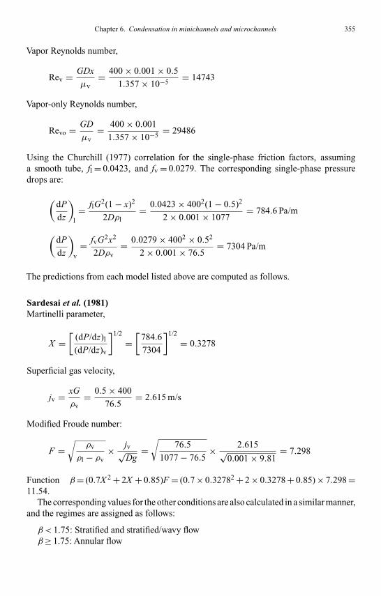
Kandlikar I044527-Ch06.tex 26/10/2005 18: 15 Page 355
Chapter 6. Condensation in minichannels and microchannels 355
Vapor Reynolds number,
Rev = GDx
µv= 400 × 0.001 × 0.5
1.357 × 10−5 = 14743
Vapor-only Reynolds number,
Revo = GD
µv= 400 × 0.001
1.357 × 10−5 = 29486
Using the Churchill (1977) correlation for the single-phase friction factors, assuminga smooth tube, fl = 0.0423, and fv = 0.0279. The corresponding single-phase pressuredrops are:
(dP
dz
)l= flG2(1 − x)2
2Dρl= 0.0423 × 4002(1 − 0.5)2
2 × 0.001 × 1077= 784.6 Pa/m
(dP
dz
)v
= fvG2x2
2Dρv= 0.0279 × 4002 × 0.52
2 × 0.001 × 76.5= 7304 Pa/m
The predictions from each model listed above are computed as follows.
Sardesai et al. (1981)Martinelli parameter,
X =[
(dP/dz)l
(dP/dz)v
]1/2
=[
784.6
7304
]1/2
= 0.3278
Superficial gas velocity,
jv = xG
ρv= 0.5 × 400
76.5= 2.615 m/s
Modified Froude number:
F =√
ρv
ρl − ρv× jv√
Dg=√
76.5
1077 − 76.5× 2.615√
0.001 × 9.81= 7.298
Function β= (0.7X 2 + 2X + 0.85)F = (0.7 × 0.32782 + 2 × 0.3278 + 0.85) × 7.298 =11.54.
The corresponding values for the other conditions are also calculated in a similar manner,and the regimes are assigned as follows:
β< 1.75: Stratified and stratified/wavy flowβ≥ 1.75: Annular flow
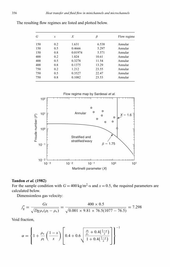
Kandlikar I044527-Ch06.tex 26/10/2005 18: 15 Page 356
356 Heat transfer and fluid flow in minichannels and microchannels
The resulting flow regimes are listed and plotted below.
G x X β Flow regime
150 0.2 1.631 6.538 Annular150 0.5 0.4666 5.297 Annular150 0.8 0.01974 5.571 Annular400 0.2 1.024 10.61 Annular400 0.5 0.3278 11.54 Annular400 0.8 0.1375 13.29 Annular750 0.2 1.212 23.55 Annular750 0.5 0.3527 22.47 Annular750 0.8 0.1082 23.53 Annular
10�3
10�1
10�2
102
101
100
10�2 10�1
Martinelli parameter (X)
Stratified andstratified/wavy
Annular X � 1.6
b � 1.75
Flow regime map by Sardesai et al.
Fro
ude
num
ber
(F)
100 101
Tandon et al. (1982)For the sample condition with G = 400 kg/m2-s and x = 0.5, the required parameters arecalculated below.
Dimensionless gas velocity:
j∗g = Gx√Dgρv(ρl − ρv)
= 400 × 0.5√0.001 × 9.81 × 76.5(1077 − 76.5)
= 7.298
Void fraction,
α =
1 + ρv
ρl
(1 − x
x
)0.4 + 0.6
√√√√ ρlρv
+ 0.4( 1−x
x
)1 + 0.4
( 1−xx
)
−1

Kandlikar I044527-Ch06.tex 26/10/2005 18: 15 Page 357
Chapter 6. Condensation in minichannels and microchannels 357
⇒ α =1 + 76.5
1077
(1 − 0.5
0.5
)0.4 + 0.6
√√√√ 107776.5 + 0.4
( 1−0.50.5
)1 + 0.4
( 1−0.50.5
)
−1
= 0.858
⇒ 1 − α
α= 0.1654
In a similar manner, these parameters are computed for each of the conditions, and theflow regimes assigned according to the transition criteria listed in Section 6.2.2.
G x j∗g1 − α
αFlow regime
150 0.2 1.095 0.5322 Undesignated150 0.5 2.737 0.1654 Annular and semi-annular150 0.8 4.379 0.04535 Annular and semi-annular400 0.2 2.919 0.5322 Undesignated400 0.5 7.298 0.1654 Spray400 0.8 11.68 0.04535 Spray750 0.2 5.473 0.5322 Undesignated750 0.5 13.68 0.1654 Spray750 0.8 21.89 0.04535 Spray
Flow regime map by Tandon et al.
Spray
Wavy
6.0
1.0
0.5
10
10
1
1
0.1
0.1
0.01
0.010.001
0.001
0.5
0.01
Slug
Plug
Annular andsemi-annular
1 � aa
j g*
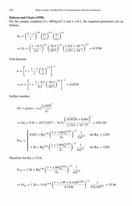
Kandlikar I044527-Ch06.tex 26/10/2005 18: 15 Page 358
358 Heat transfer and fluid flow in minichannels and microchannels
Dobson and Chato (1998)For the sample condition G = 400 kg/m2-s and x = 0.5, the required parameters are asfollows.
Xtt =(
1 − x
x
)0.9 (ρv
ρl
)0.5 (µl
µg
)0.1
⇒ Xtt =(
1 − 0.5
0.5
)0.9 ( 76.5
1077
)0.5 (1.321 × 10⁻⁴
1.357 × 10⁻⁵
)0.1
= 0.3346
Void fraction:
α =[
1 + 1 − x
x
(ρv
ρl
)2/3]−1
⇒ α =[
1 + 1 − 0.5
0.5
(76.5
1077
)2/3]−1
= 0.8536
Galileo number,
Ga = gρl(ρl − ρv)
(√αD)3
µ2l
⇒ Ga = 9.81 × 1077(1077 − 76.5)
(√0.8536 × 0.001
)3
(1.321 × 10⁻⁴)2 = 478,182
Frso =
0.025 × Re1.59l
(1 + 1.09X 0.039
tt
Xtt
)1.51
Ga0.5 for Rel ≤ 1250
1.26 × Re1.04l
(1 + 1.09X 0.039
tt
Xtt
)1.51
Ga0.5 for Rel > 1250
Therefore for Rel = 1514,
Frso = 1.26 × Re1.04l
(1 + 1.09X 0.039
tt
Xtt
)1.51
Ga0.5
⇒ Frso = 1.26 × 15141.04(
1 + 1.09 × 0.33460.039
0.3346
)1.51
478,1820.5 = 55.86

Kandlikar I044527-Ch06.tex 26/10/2005 18: 15 Page 359
Chapter 6. Condensation in minichannels and microchannels 359
In a similar manner, these parameters are computed for each of the conditions, and theflow regimes assigned according to the transition criteria based on Frso and G listed inSection 6.2.2. The respective flow regimes are follows:
G x Frso Flow regime
150 0.2 5.797 Wavy150 0.5 13.08 Wavy150 0.8 17.49 Wavy400 0.2 19.12 Wavy400 0.5 55.86 Annular400 0.8 83.17 Annular750 0.2 36.77 Annular750 0.5 107.4 Annular750 0.8 226 Annular
0.0 0.2
Mas
s flu
x, G
(kg
/m2 -
s)
500 kg/m2-s
0.4 0.6Quality (x)
Frso � 10
Frso � 20
Flow regime map by Dobson and Chato
Annular
Wavy
800
600
400
200
00.8 1.0
Breber et al. (1980)For the sample condition G = 400 kg/m2-s and x = 0.5, the dimensionless gas velocity,j∗g = 7.298, and the Martinelli parameter Xtt = 0.3346 from the calculations above. Therespective flow regimes are assigned based on the specific values of these parameters asshown below.
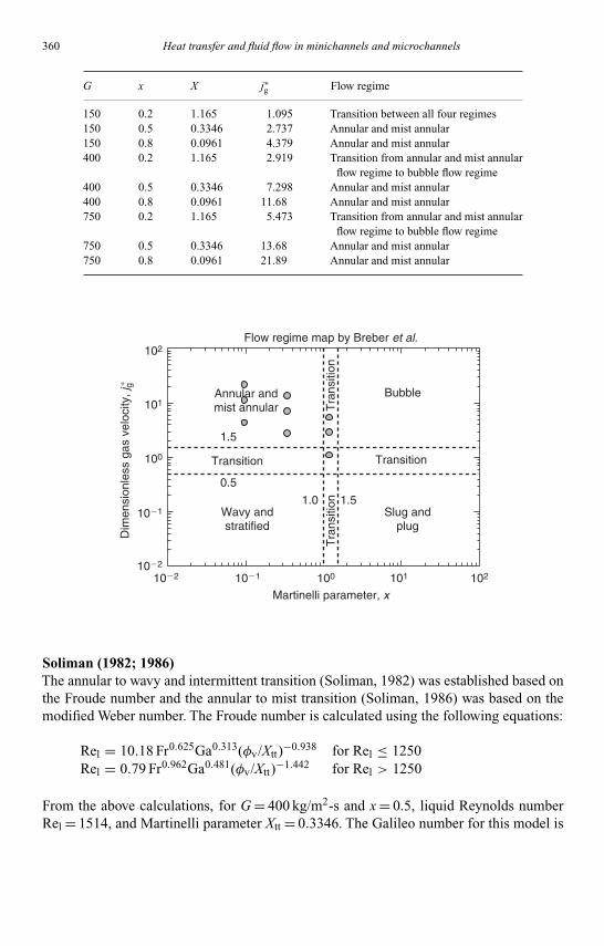
Kandlikar I044527-Ch06.tex 26/10/2005 18: 15 Page 360
360 Heat transfer and fluid flow in minichannels and microchannels
G x X j∗g Flow regime
150 0.2 1.165 1.095 Transition between all four regimes150 0.5 0.3346 2.737 Annular and mist annular150 0.8 0.0961 4.379 Annular and mist annular400 0.2 1.165 2.919 Transition from annular and mist annular
flow regime to bubble flow regime400 0.5 0.3346 7.298 Annular and mist annular400 0.8 0.0961 11.68 Annular and mist annular750 0.2 1.165 5.473 Transition from annular and mist annular
flow regime to bubble flow regime750 0.5 0.3346 13.68 Annular and mist annular750 0.8 0.0961 21.89 Annular and mist annular
102Flow regime map by Breber et al.
Martinelli parameter, x
Annular andmist annular
Transition
Wavy andstratified
Slug andplug
Transition
Tra
nsiti
onT
rans
ition
Bubble101
100
10�1
10�2
10�2 10�1
0.5
1.0 1.5
1.5
100 101 102
Dim
ensi
onle
ss g
as v
eloc
ity, j
g∗
Soliman (1982; 1986)The annular to wavy and intermittent transition (Soliman, 1982) was established based onthe Froude number and the annular to mist transition (Soliman, 1986) was based on themodified Weber number. The Froude number is calculated using the following equations:
Rel = 10.18 Fr0.625Ga0.313(φv/Xtt)−0.938 for Rel ≤ 1250Rel = 0.79 Fr0.962Ga0.481(φv/Xtt)−1.442 for Rel > 1250
From the above calculations, for G = 400 kg/m2-s and x = 0.5, liquid Reynolds numberRel = 1514, and Martinelli parameter Xtt = 0.3346. The Galileo number for this model is
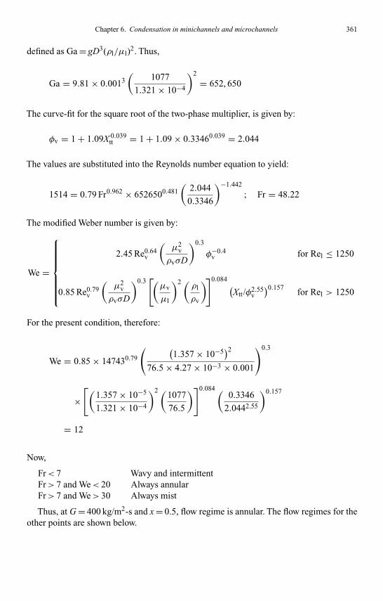
Kandlikar I044527-Ch06.tex 26/10/2005 18: 15 Page 361
Chapter 6. Condensation in minichannels and microchannels 361
defined as Ga = gD3(ρl/µl)2. Thus,
Ga = 9.81 × 0.0013(
1077
1.321 × 10⁻⁴
)2
= 652, 650
The curve-fit for the square root of the two-phase multiplier, is given by:
φv = 1 + 1.09X 0.039tt = 1 + 1.09 × 0.33460.039 = 2.044
The values are substituted into the Reynolds number equation to yield:
1514 = 0.79 Fr0.962 × 6526500.481(
2.044
0.3346
)−1.442
; Fr = 48.22
The modified Weber number is given by:
We =
2.45 Re0.64v
(µ2
v
ρvσD
)0.3
φ−0.4v for Rel ≤ 1250
0.85 Re0.79v
(µ2
v
ρvσD
)0.3[(
µv
µl
)2 (ρl
ρv
)]0.084 (Xtt/φ2.55
v
)0.157for Rel > 1250
For the present condition, therefore:
We = 0.85 × 147430.79
( (1.357 × 10⁻⁵
)276.5 × 4.27 × 10−3 × 0.001
)0.3
×[(
1.357 × 10⁻⁵
1.321 × 10⁻⁴
)2 (1077
76.5
)]0.084 (0.3346
2.0442.55
)0.157
= 12
Now,
Fr< 7 Wavy and intermittentFr> 7 and We< 20 Always annularFr> 7 and We> 30 Always mist
Thus, at G = 400 kg/m2-s and x = 0.5, flow regime is annular. The flow regimes for theother points are shown below.

Kandlikar I044527-Ch06.tex 26/10/2005 18: 15 Page 362
362 Heat transfer and fluid flow in minichannels and microchannels
G x Fr We Flow regime
150 0.2 3.908 3.36 Wavy and intermittent150 0.5 11.54 6.10 Annular150 0.8 16.7 8.324 Annular400 0.2 12.58 7.008 Annular400 0.5 48.22 12.00 Annular400 0.8 80.20 15.59 Annular750 0.2 24.17 11.52 Annular750 0.5 92.68 19.72 Annular750 0.8 219.3 23.32 Annular/mist transition
Wavyand intermittent
Annular
Mist
0.0 0.2 0.4 0.6Quality (x)
Mas
s flu
x, G
(kg
/m2 -
s)
Fr � 7
We � 20
We � 30
2000
1500
Flow regime map by Soliman
1000
500
00.8 1.0
Laminar (Re1 < 1250)Turbulent (Re1 > 1250)
Coleman and Garimella (2000b; 2000a; 2003) and Garimella (2004)Simple algebraic curve-fits to their G-x transition lines are given below.
Intermittent flow to intermittent and annular film flow:
G = 547.7 − 1227x
1 + 2.856x
Intermittent and annular film flow to annular film flow:
G = −56.13 + 125.4/x
Annular film flow to annular film and mist flow:
G = 206.1 + 85.8/x

Kandlikar I044527-Ch06.tex 26/10/2005 18: 15 Page 363
Chapter 6. Condensation in minichannels and microchannels 363
Annular film and mist flow to mist flow:
G = 207.2 − 527.5x
1 − 1.774x
Dispersed bubble flow:
G = 1376 − 97.1/x
The respective lines and the conditions of interest are shown in the graph below.Thus, the flow regimes are assigned as follows:
G x Flow regime
150 0.2 Intermittent flow150 0.5 Intermittent and annular film flow150 0.8 Annular film flow400 0.2 Intermittent and annular film flow400 0.5 Annular film and mist flow400 0.8 Annular film and mist flow750 0.2 Annular film and mist flow750 0.5 Annular film and mist flow750 0.8 Mist flow
Flow regime map by Coleman and Garimella
Quality (x)
0.0 0.1 0.2
800
700
600
Annular filmand mist flow
Annular film flow
Plug/slug andannular film flow
Mas
s flu
x, G
(kg
/m2 -
s)
Plug/slugflow
Dispersedbubble
flow
Mist flow
500
400
300
200
1000.3 0.4 0.5 0.6 0.7 0.8 0.9 1.0
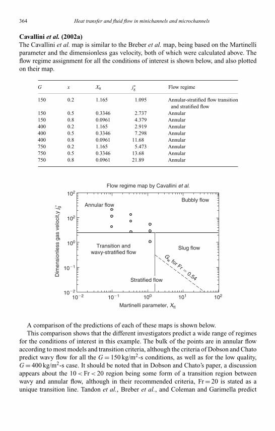
Kandlikar I044527-Ch06.tex 26/10/2005 18: 15 Page 364
364 Heat transfer and fluid flow in minichannels and microchannels
Cavallini et al. (2002a)The Cavallini et al. map is similar to the Breber et al. map, being based on the Martinelliparameter and the dimensionless gas velocity, both of which were calculated above. Theflow regime assignment for all the conditions of interest is shown below, and also plottedon their map.
G x Xtt j∗g Flow regime
150 0.2 1.165 1.095 Annular-stratified flow transitionand stratified flow
150 0.5 0.3346 2.737 Annular150 0.8 0.0961 4.379 Annular400 0.2 1.165 2.919 Annular400 0.5 0.3346 7.298 Annular400 0.8 0.0961 11.68 Annular750 0.2 1.165 5.473 Annular750 0.5 0.3346 13.68 Annular750 0.8 0.0961 21.89 Annular
102
102
100
10�1
10�2
10�2 10�1
Martinelli parameter, Xtt
100 101 102
Flow regime map by Cavallini et al.
Dim
ensi
onle
ss g
as v
eloc
it,y
j g Annular flowBubbly flow
Transition andwavy-stratified flow
Slug flowG
w for Fr � 0.54Stratified flow
∗
A comparison of the predictions of each of these maps is shown below.This comparison shows that the different investigators predict a wide range of regimes
for the conditions of interest in this example. The bulk of the points are in annular flowaccording to most models and transition criteria, although the criteria of Dobson and Chatopredict wavy flow for all the G = 150 kg/m2-s conditions, as well as for the low quality,G = 400 kg/m2-s case. It should be noted that in Dobson and Chato’s paper, a discussionappears about the 10<Fr< 20 region being some form of a transition region betweenwavy and annular flow, although in their recommended criteria, Fr = 20 is stated as aunique transition line. Tandon et al., Breber et al., and Coleman and Garimella predict

Kandlikar I044527-Ch06.tex 26/10/2005 18: 15 Page 365
Chapter 6. Condensation in minichannels and microchannels 365
some form of mist flow, either in combination with annular flow, or by itself, at the highermass fluxes and qualities. The similarities in the bases between the Breber et al. andCavallini et al. maps are also evident in this table. Of these maps, only the Coleman andGarimella criteria are reported to apply for condensation in tubes as small as 1 mm, whilethe Dobson and Chato criteria apply down to D = 3.14 mm, and many of the other criteriawere for tubes with D> 4.8 mm, with most being primarily based on tubes with D ≥ 8 mm.Flow regime studies for the channels much smaller than 1 mm were not represented in theabove illustration because they are all for adiabatic air–water or nitrogen–water flow, andmany of them do not propose explicit transition equations.
DobsonSardesai Tandon and Breber Cavallini Coleman and
Condition et al. et al. Chato et al. Soliman et al. Garimella
G = 150 kg/m2-s Annular – Wavy Transition Wavy and Annular- Plug/slug flowx = 0.2 between intermittent stratified
all four flowregimes transition
and stratifiedflow
G = 150 kg/m2-s Annular Annular and Wavy Annular Annular Annular Plug/slug andx = 0.5 semi-annular and mist annular
annular film flowG = 150 kg/m2-s Annular Annular and Wavy Annular Annular Annular Annularx = 0.8 semi-annular and mist film flow
annularG = 400 kg/m2-s Annular – Wavy Transition Annular Annular Plug/slug andx = 0.2 from annular film
annular flowand mistannular flowregime tobubble flowregime
G = 400 kg/m2-s Annular Spray Annular Annular Annular Annular Annular filmx = 0.5 and mist and mist flow
annularG = 400 kg/m2-s Annular Spray Annular Annular Annular Annular Annular filmx = 0.8 and mist and mist flow
annularG = 750 kg/m2-s Annular – Annular Transition Annular Annular Annular filmx = 0.2 from and mist flow
annularand mistannular flowregime tobubble flowregime
G = 750 kg/m2-s Annular Spray Annular Annular Annular Annular Annular filmx = 0.5 and mist and mist flow
annularG = 750 kg/m2-s Annular Spray Annular Annular Transition Annular Mist flowx = 0.8 and mist
annular

Kandlikar I044527-Ch06.tex 26/10/2005 18: 15 Page 366
366 Heat transfer and fluid flow in minichannels and microchannels
Example 6.2. Void fraction calculation
Compute the void fraction for refrigerant R-134a flowing through a 1-mm tube at a pressureof 1500 kPa, at mass fluxes 150, 400, and 750 kg/m2-s and qualities of 0.2, 0.5, and 0.8.Use the homogeneous model and correlations by Kawahara et al. (2002), Baroczy (1965),Zivi (1964), Lockhart and Martinelli (1949), Thom (1964), Steiner (1993), Tandon et al.(1985b), El Hajal et al. (2003), Smith (1969), Premoli et al. (1971), and Yashar et al.(2001). Compare the values predicted by each model and comment.
Refrigerant propertiesSaturation temperature: Tsat = 55.21◦CSurface tension: σ= 4.27 × 10⁻³ N/mRepresentative calculations are shown here for the G = 400 kg/m2-s, x = 0.5 case.
Liquid phase Vapor phase
ρl = 1077 kg/m3 ρv = 76.5 kg/m3
µl = 1.321 × 10⁻⁴ kg/m-s µv = 1.357 × 10⁻⁵ kg/m-s
Homogeneous modelThe void fraction is given by:
α =[
1 + 1 − x
x
(ρv
ρl
)]−1
=[
1 + 1 − 0.5
0.5
(76.5
1077
)]−1
= 0.9337
Some investigators, for example, Triplett et al. (1999a) recommend the homogeneousmodel for calculation of void fraction in channels with Dh ∼ 1 mm.
Kawahara et al. (2002)Kawahara et al. (2002) recommend the following correlation for void fraction in tubes ofdiameters 100 and 50 µm.
α = C1α0.5h
1 − C2α0.5h
where, αh is the homogeneous void fraction
C1 ={
0.03 For D = 100 µm0.02 For D = 50 µm
and C2 ={
0.97 For D = 100 µm0.98 For D = 50 µm
Based on experimental data, they recommend that for D> 250 µm, the void fraction becomputed using the homogeneous model. Therefore, for this case (D = 1 mm), the voidfraction is 0.9337.

Kandlikar I044527-Ch06.tex 26/10/2005 18: 15 Page 367
Chapter 6. Condensation in minichannels and microchannels 367
Baroczy (1965)The Baroczy void fraction is calculated as follows:
α =[
1 +(
1 − x
x
)0.74 (ρv
ρl
)0.65 (µl
µv
)0.13]−1
⇒ α =[
1 +(
1 − 0.5
0.5
)0.74 ( 76.5
1077
)0.65 (1.321 × 10⁻⁴
1.357 × 10⁻⁵
)0.13]−1
= 0.8059
Koyama et al. (2004) recommend this correlation for smooth tubes, but mention that itdoes not predict the void fraction in microfin tubes well.
Zivi (1964)This widely used correlation is given by:
α =[
1 + 1 − x
x
(ρv
ρl
)2/3]−1
⇒ α =[
1 + 1 − 0.5
0.5
(76.5
1077
)2/3]−1
= 0.8536
Lockhart and Martinelli (1949)This correlation is given by:
α =[
1 + 0.28(
1 − x
x
)0.64 (ρv
ρl
)0.36 (µl
µv
)0.07]−1
⇒ α =[
1 + 0.28(
1 − 0.5
0.5
)0.64 ( 76.5
1077
)0.36 (1.321 × 10⁻⁴
1.357 × 10⁻⁵
)0.07]−1
= 0.8875
Based on experimental data for air–water flow in 6.6 and 33.2 mm diameter tubes,Ekberg et al. (1999) recommend the Lockhart and Martinelli correlation for void fractioncalculations.
Thom (1964)The calculation is as follows:
α =[
1 +(
1 − x
x
)(ρv
ρl
)0.89 (µl
µv
)0.18]−1
⇒ α =[
1 +(
1 − 0.5
0.5
)(76.5
1077
)0.89 (1.321 × 10⁻⁴
1.357 × 10⁻⁵
)0.18]−1
= 0.8748

Kandlikar I044527-Ch06.tex 26/10/2005 18: 15 Page 368
368 Heat transfer and fluid flow in minichannels and microchannels
Steiner (1993)
α = x
ρv
([1 + 0.12(1 − x)]
[x
ρv+ 1 − x
ρl
]+ 1.18(1 − x) [g × σ(ρl − ρv)]0.25
G × ρ0.5l
)−1
⇒ α = 0.5
76.5
([1 + 0.12(1 − 0.5)]
[0.5
76.5+ 1 − 0.5
1077
]
+ 1.18(1 − 0.5)[9.81 × 4.27 × 10−3 × (1077 − 76.5)
]0.25
400 × 10770.5
)−1
The resulting void fraction is α= 0.8675.
Tandon et al. (1985b)The liquid Reynolds number required for this correlation is given by:
Rel = GD(1 − x)
µl= 400 × 0.001 × (1 − 0.5)
1.321 × 10−4 = 1514
The Martinelli parameter is given by:
Xtt =(
1 − x
x
)0.9 (ρv
ρl
)0.5 (µl
µv
)0.1
=(
1 − 0.5
0.5
)0.9 ( 76.5
1077
)0.5 (1.321 × 10⁻⁴
1.357 × 10⁻⁵
)0.1
= 0.3346
The parameter F is given by:
F(Xtt) = 0.15 [X −1tt + 2.85 X −0.476
tt ]
⇒ F(Xtt) = 0.15[0.3346−1 + 2.85 × 0.3346−0.476] = 1.168
The void fraction is given by:
α ={
1 − 1.928 Re−0.315l [F(Xtt)]−1 + 0.9293 Re−0.315
l [F(Xtt)]−2 50 < Rel < 1125
1 − 0.38 Re−0.088l [F(Xtt)]−1 + 0.0361 Rel
−0.176[F(Xtt)]−2 Rel > 1125
In the present case:
α = 1 − 0.38 × 1514−0.088[1.168]−1 + 0.0361 × 1514−0.176[1.168]−2 = 0.8365
El Hajal et al. (2003)El Hajal et al. (2003) proposed the following correlation that uses the void fractioncalculated by the homogeneous model and the correlation by Steiner (1993).
α = αh − αSteiner
ln(
αhαSteiner
)

Kandlikar I044527-Ch06.tex 26/10/2005 18: 15 Page 369
Chapter 6. Condensation in minichannels and microchannels 369
where αh and αSteiner are the void fractions calculated by the homogeneous model andthe correlation by Steiner (1993). In the present case, αh = 0.9337, and αSteiner = 0.8675.Therefore,
α = 0.9337 − 0.8675
ln( 0.9337
0.8675
) = 0.9002
Smith (1969)This correlation is given by:
α =
1 +
(ρv
ρl
)(1 − x
x
)×K + (1 − K)
√√√√(ρlρv
)+ K
( 1−xx
)1 + K
( 1−xx
)
−1
Smith found good agreement with experimental data (air–water and steam–water, 6–38-mm diameter tubes) for K = 0.4. In the present case:
α =1 +
(76.5
1077
)(1 − 0.5
0.5
)×0.4 + (1 − 0.4)
√√√√( 107776.5
)+ 0.4( 1−0.5
0.5
)1 + 0.4
( 1−0.50.5
)
−1
= 0.858
Tabatabai and Faghri (2001) found the best agreement with their data for 4.8–15.88-mmtubes (refrigerants) and 1–12.3-mm tubes (air–water) with the Smith and Lockhart–Martinelli correlations. They preferred the Smith correlation for its wide range ofapplicability.
Premoli et al. (1971)The liquid-only Reynolds number is given by:
Relo = GD
µl= 400 × 1 × 10−3
1.321 × 10−4 = 3028
The liquid-only Weber number is given by:
Welo = G2D
σρl= 4002 × 1 × 10−3
0.00427 × 1077= 34.78
The parameters E1 and E2 are calculated as follows:
E1 = 1.578 Re−0.19lo
(ρl
ρv
)0.22
= 1.578 × 3028−0.19 ×(
1077
76.5
)0.22
= 0.6157
E2 = 0.0273 WeloRe−0.51lo
(ρl
ρv
)−0.08
= 0.0273 × 34.78
× 3028−0.51 ×(
1077
76.5
)−0.08
= 0.01289
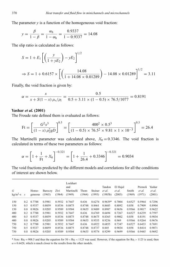
Kandlikar I044527-Ch06.tex 26/10/2005 18: 15 Page 370
370 Heat transfer and fluid flow in minichannels and microchannels
The parameter y is a function of the homogeneous void fraction:
y = β
1 − β= αh
1 − αh= 0.9337
1 − 0.9337= 14.08
The slip ratio is calculated as follows:
S = 1 + E1
[(y
1 + yE2
)− yE2
]1/2
⇒ S = 1 + 0.6157 ×[(
14.08
1 + 14.08 × 0.01289
)− 14.08 × 0.01289
]1/2
= 3.11
Finally, the void fraction is given by:
α = x
x + S(1 − x) ρv/ρl= 0.5
0.5 + 3.11 × (1 − 0.5) × 76.5/1077= 0.8191
Yashar et al. (2001)The Froude rate defined them is evaluated as follows:
Ft =[
G2x3
(1 − x) ρ2vgD
]0.5
=[
4002 × 0.53
(1 − 0.5)× 76.52 × 9.81 × 1 × 10−3
]0.5
= 26.4
The Martinelli parameter was calculated above, Xtt = 0.3346. The void fraction iscalculated in terms of these two parameters as follows:
α =[
1 + 1
Ft+ Xtt
]−0.321
=[
1 + 1
26.4+ 0.3346
]−0.321
= 0.9034
The void fractions predicted by the different models and correlations for all the conditionsof interest are shown below.
Lockhartand Tandon El Hajal Premoli Yashar
G Homo- Baroczy Zivi Martinelli Thom Steiner et al. et al. Smith et al. et al.kg/m2-s x geneous (1965) (1964) (1949) (1964) (1993) (1985b) (2003) (1969) (1971) (2001)
150 0.2 0.7788 0.5981 0.5932 0.7647 0.636 0.6274 0.9639* 0.7004 0.6527 0.5964 0.7296150 0.5 0.9337 0.8059 0.8536 0.8875 0.8748 0.8461 0.8685 0.8892 0.858 0.7909 0.8904150 0.8 0.9826 0.9205 0.9589 0.9504 0.9655 0.9489 0.8987 0.9656 0.9566 0.9017 0.9622400 0.2 0.7788 0.5981 0.5932 0.7647 0.636 0.6769 0.6694 0.7267 0.6527 0.6239 0.7597400 0.5 0.9337 0.8059 0.8536 0.8875 0.8748 0.8675 0.8365 0.9002 0.858 0.8191 0.9034400 0.8 0.9826 0.9205 0.9589 0.9504 0.9655 0.9555 0.9256 0.969 0.9566 0.9264 0.9676750 0.2 0.7788 0.5981 0.5932 0.7647 0.636 0.6922 0.6855 0.7347 0.6527 0.6433 0.7691750 0.5 0.9337 0.8059 0.8536 0.8875 0.8748 0.8737 0.845 0.9034 0.858 0.8414 0.9071750 0.8 0.9826 0.9205 0.9589 0.9504 0.9655 0.9574 0.9299 0.9699 0.9566 0.9445 0.9692
* Note: Rel = 908.5 and thus the equation for 50<Rel < 1125 was used. However, if the equation for Rel > 1125 is used, thenα= 0.6428, which is much closer to the results from the other models.

Kandlikar I044527-Ch06.tex 26/10/2005 18: 15 Page 371
Chapter 6. Condensation in minichannels and microchannels 371
The results shown above indicate that the void fractions predicted by several of the modelsare quite close to each other. A graph depicting these values is shown in Section 6.3. Cautionmust be exercised, however, because, as stated by El Hajal et al. (2003) and Thome et al.(2003), (1 −α) is an indicator of the film thickness in annular flow, and small changes invoid fraction imply large changes in liquid film thickness, which therefore alters the heattransfer coefficient. It should also be noted that many of the correlations assume annularflow, and although some of the authors recommend that they can be used irrespective of theflow regime, in the flow regimes specific to microchannels, this should be validated further.
Example 6.3. Pressure drop calculation
Compute the frictional pressure gradient during condensation of refrigerant R-134a flowingthrough a 1 mm diameter tube, at a mass flux of 300 kg/m2-s, at a mean quality of 0.5 anda pressure of 1500 kPa. Use the correlations by Lockhart and Martinelli (1949), Friedel(1979; 1980), Chisholm (1973), Mishima and Hibiki (1996), Lee and Lee (2001), Tranet al. (2000), Wang et al. (1997b), Chen et al. (2001), Wilson et al. (2003), Souza et al.(1993), Cavallini et al. (2001; 2002a; 2002b), and Garimella et al. (2005) and comparethe values predicted by each model.
Refrigerant propertiesSaturation temperature Tsat = 55.21◦CSurface tension σ= 0.00427 N/m
Liquid phase Vapor phase
ρl = 1077 kg/m3 ρv = 76.5 kg/m3
µl = 1.321 × 10⁻⁴ kg/m-s µv = 1.357 × 10⁻⁵ kg/m-s
Some common parameters that are used by several correlations are calculated belowfirst.
Liquid Reynolds number,
Rel = GD(1 − x)
µl= 300 × 0.001 × (1 − 0.5)
1.321 × 10−4 = 1136
Vapor Reynolds number,
Rev = GDx
µv= 300 × 0.001 × 0.5
1.357 × 10−5 = 11054
Liquid-only Reynolds number,
Relo = GD
µl= 300 × 0.001
1.321 × 10−4 = 2271
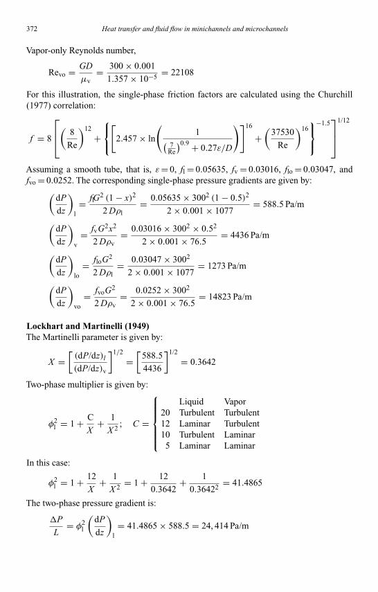
Kandlikar I044527-Ch06.tex 26/10/2005 18: 15 Page 372
372 Heat transfer and fluid flow in minichannels and microchannels
Vapor-only Reynolds number,
Revo = GD
µv= 300 × 0.001
1.357 × 10−5 = 22108
For this illustration, the single-phase friction factors are calculated using the Churchill(1977) correlation:
f = 8
( 8
Re
)12
+[
2.457 × ln
(1( 7
Re
)0.9 + 0.27ε/D
)]16
+(
37530
Re
)16
−1.5
1/12
Assuming a smooth tube, that is, ε= 0, fl = 0.05635, fv = 0.03016, flo = 0.03047, andfvo = 0.0252. The corresponding single-phase pressure gradients are given by:(
dP
dz
)l= flG2 (1 − x)2
2 Dρl= 0.05635 × 3002 (1 − 0.5)2
2 × 0.001 × 1077= 588.5 Pa/m
(dP
dz
)v
= fvG2x2
2 Dρv= 0.03016 × 3002 × 0.52
2 × 0.001 × 76.5= 4436 Pa/m
(dP
dz
)lo
= floG2
2 Dρl= 0.03047 × 3002
2 × 0.001 × 1077= 1273 Pa/m
(dP
dz
)vo
= fvoG2
2 Dρv= 0.0252 × 3002
2 × 0.001 × 76.5= 14823 Pa/m
Lockhart and Martinelli (1949)The Martinelli parameter is given by:
X =[(dP/dz)l(dP/dz)v
]1/2
=[
588.5
4436
]1/2
= 0.3642
Two-phase multiplier is given by:
φ2l = 1 + C
X+ 1
X 2 ; C =
Liquid Vapor20 Turbulent Turbulent12 Laminar Turbulent10 Turbulent Laminar
5 Laminar Laminar
In this case:
φ2l = 1 + 12
X+ 1
X 2 = 1 + 12
0.3642+ 1
0.36422 = 41.4865
The two-phase pressure gradient is:
P
L= φ2
l
(dP
dz
)l= 41.4865 × 588.5 = 24, 414 Pa/m

Kandlikar I044527-Ch06.tex 26/10/2005 18: 15 Page 373
Chapter 6. Condensation in minichannels and microchannels 373
Friedel (1979; 1980)The parameters E, F , and H are evaluated as follows:
E = (1 − x)2 + x2 ρl fvo
ρvflo
⇒ E = (1 − 0.5)2 + 0.52 × 1077 × 0.0252
76.5 × 0.03047= 3.161
F = x0.78 × (1 − x)0.24 = 0.50.78 × (1 − 0.5)0.24 = 0.4931
H =(ρl
ρv
)0.91 (µv
µl
)0.19 (1 − µv
µl
)0.7
⇒ H =(
1077
76.5
)0.91 (1.357 × 10⁻⁵
1.321 × 10⁻⁴
)0.19 (1 − 1.357 × 10⁻⁵
1.321 × 10⁻⁴
)0.7
= 6.677
The two-phase mixture density is calculated as follows:
ρTP =(
x
ρv+ 1 − x
ρl
)−1
=(
0.5
76.5+ 1 − 0.5
1077
)−1
= 142.8 kg/m3
The Froude and Weber numbers are given by:
Fr = G2
gDρ2TP
= 3002
9.81 × 0.001 × 142.82 = 449.6
We = G2D
ρTPσ= 3002 × 0.001
142.8 × 4.27 × 10−3 = 147.5
The resulting two-phase multiplier is now calculated as follows:
φ2lo = E + 3.24 × FH
Fr0.045 We0.035 = 3.161 + 3.24 × 0.4931 × 6.677
449.60.045 × 147.50.035 = 9.967
Finally, the two-phase pressure gradient is given by:
P
L= φ2
lo
(P
L
)lo
= 9.967 × 1273 = 12, 688 Pa/m
Chisholm (1973)The ratio of the vapor- to liquid-only pressure gradients is given by:
Y =√(dP/dz)vo
(dP/dz)lo=√
14,823
1273= 3.412
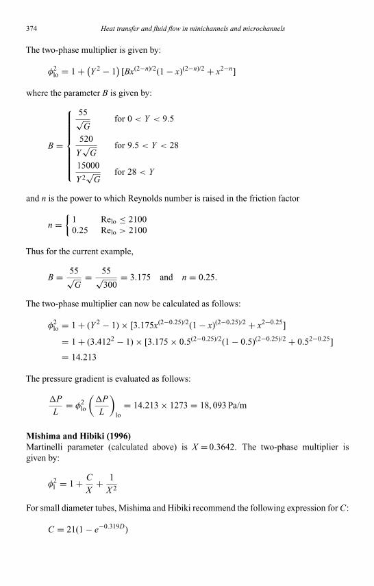
Kandlikar I044527-Ch06.tex 26/10/2005 18: 15 Page 374
374 Heat transfer and fluid flow in minichannels and microchannels
The two-phase multiplier is given by:
φ2lo = 1 + (
Y 2 − 1)
[Bx(2−n)/2(1 − x)(2−n)/2 + x2−n]
where the parameter B is given by:
B =
55√G
for 0 < Y < 9.5
520
Y√
Gfor 9.5 < Y < 28
15000
Y 2√
Gfor 28 < Y
and n is the power to which Reynolds number is raised in the friction factor
n ={
1 Relo ≤ 21000.25 Relo > 2100
Thus for the current example,
B = 55√G
= 55√300
= 3.175 and n = 0.25.
The two-phase multiplier can now be calculated as follows:
φ2lo = 1 + (Y 2 − 1) × [3.175x(2−0.25)/2(1 − x)(2−0.25)/2 + x2−0.25]
= 1 + (3.4122 − 1) × [3.175 × 0.5(2−0.25)/2(1 − 0.5)(2−0.25)/2 + 0.52−0.25]
= 14.213
The pressure gradient is evaluated as follows:
P
L= φ2
lo
(P
L
)lo
= 14.213 × 1273 = 18, 093 Pa/m
Mishima and Hibiki (1996)Martinelli parameter (calculated above) is X = 0.3642. The two-phase multiplier isgiven by:
φ2l = 1 + C
X+ 1
X 2
For small diameter tubes, Mishima and Hibiki recommend the following expression for C:
C = 21(1 − e−0.319D)

Kandlikar I044527-Ch06.tex 26/10/2005 18: 15 Page 375
Chapter 6. Condensation in minichannels and microchannels 375
⇒ C = 21(1 − e−0.319×1) = 5.736
With this value of C, the two-phase multiplier is given by:
⇒ φ2l = 1 + 5.736
X+ 1
X 2 = 1 + 5.736
0.3642+ 1
0.36422 = 24.285
The two-phase pressure gradient is then calculated as follows:
P
L= φ2
l
(dP
dz
)l= 24.285 × 588.5 = 14,292 Pa/m
Lee and Lee (2001)The Martinelli parameter, calculated above is X = 0.3642. For the C parameter in the two-
phase multiplier, Lee and Lee suggested C = A λq ψr Reslo, where, λ= µ2
lρlσD , ψ= µl j
σ, and
j = liquid slug velocity, also given by j = jV + jL. The value of constants A, q, r, and s aredetermined based on the following Table:
Flow regime
Liquid Vapor A q r s X -Range Relo Range
Laminar Laminar 6.833 × 10⁻⁸ −1.317 0.719 0.557 0.776–14.176 175–1480Laminar Turbulent 6.185 × 10⁻² 0 0 0.726 0.303–1.426 293–1506Turbulent Laminar 3.627 0 0 0.174 3.276–79.415 2606–17642Turbulent Turbulent 0.408 0 0 0.451 1.309–14.781 2675–17757
It should be noted that surface tension effects are important only in the laminar–laminarflow regimes. For all other flow regimes, the exponents of ψ and λ are almost zero. Thus,for these flow regimes, C is merely a function of Relo. The above table also provides therange of X and Relo for the data from which these constants were determined. The liquidReynolds number for this case, calculated above, is Relo = 2271. For the current example(laminar liquid film and turbulent vapor core), the coefficient C is evaluated as follows:
C = 6.185 × 10⁻² × Re0.726lo = 6.185 × 10−2 × 22710.726 = 16.9
The two-phase multiplier is therefore:
φ2l = 1 + 16.9
X+ 1
X 2 = 1 + 16.9
0.3642+ 1
0.36422 = 54.953
Finally, the two-phase pressure gradient is calculated as follows:
P
L= φ2
l
(dP
dz
)l= 54.953 × 588.5 = 32,340 Pa/m

Kandlikar I044527-Ch06.tex 26/10/2005 18: 15 Page 376
376 Heat transfer and fluid flow in minichannels and microchannels
Tran et al. (2000)Tran et al. modified the two-phase multiplier correlation of Chisholm (1973) to thefollowing expression that includes the confinement number:
φ2lo = 1 + (
4.3Y 2 − 1)× Nconf x0.875(1 − x)0.875 + x1.75
where, confinement number is given by:
Nconf =[
σg(ρl−ρv)
]1/2
D=[
4.27×10⁻³
9.81(1077−76.5)
]1/2
0.001= 0.6595
for the current example. With Y = 3.412 calculated above,
φ2lo = 1 + (4.3 × 3.4122 − 1) × 0.6595 × 0.50.875 × (1 − 0.5)0.875 + 0.51.75 = 10.916
The two-phase pressure gradient is evaluated in the usual manner:
P
L= φ2
lo
(P
L
)lo
= 10.916 × 1273 = 13, 897 Pa/m
Wang et al. (1997b)According to their correlation, for G< 200 kg/m2-s φ2
v = 1 + 9.4X 0.62 + 0.564X 2.45.For G> 200 kg/m2-s, they modified the parameter C in the Lockhart–Martinelli (1949)correlation as follows:
C = 4.566 × 10−6X 0.128 × Re0.938lo
(ρl
ρv
)−2.15 (µl
µv
)5.1
In this example, G = 300 kg/m2-s; therefore:
C = 4.566 × 10−6 × 0.36420.128 × 22710.938(
1077
76.5
)−2.15 (1.321 × 10⁻⁴
1.357 × 10⁻⁵
)5.1
= 2.099
The two-phase multiplier is then given by:
φ2l = 1 + 2.099
X+ 1
X 2 = 1 + 2.099
0.3642+ 1
0.36422 = 14.304
And the two-phase pressure gradient is:
P
L= φ2
l
(dP
dz
)l= 14.304 × 588.5 = 8416 Pa/m

Kandlikar I044527-Ch06.tex 26/10/2005 18: 15 Page 377
Chapter 6. Condensation in minichannels and microchannels 377
Chen et al. (2001)Chen et al. modified the homogenous model and the Friedel (1979; 1980) correlation todetermine the pressure drop in microchannels. The modification to the Friedel correlationis illustrated here. Thus,
dP
dz= dP
dz
∣∣∣∣Friedel
�; � =
0.0333 × Re0.45lo
Re0.09v (1 + 0.4 exp (−Bo))
Bo < 2.5
We0.2
(2.5 + 0.06Bo)Bo ≥ 2.5
where Weber number, We = G2Dσρm
and Bond number, Bo = g(ρl − ρv)(
(D/2)2
σ
). For this
case:
Bo = g(ρl − ρv)(
(D/2)2
σ
)= 9.81(1077 − 76.5)
((0.001/2)2
4.27 × 10⁻³
)= 0.5748
Because Bo< 2.5, the modifier to the Friedel correlation is given by:
⇒ � = 0.0333 × Re0.45lo
Re0.09v (1 + 0.4 exp (−Bo))
= 0.0333 × 22710.45
110540.09(1 + 0.4 exp (−0.5748))= 0.3808
Therefore, the two-phase pressure gradient is:
dP
dz= dP
dz
∣∣∣∣Friedel
� = 12688 × 0.3808 = 4831 Pa/m
Wilson et al. (2003)Wilson et al. recommended the liquid-only two-phase multiplier of Jung and Radermacher(1989):
φ2lo = 12.82X −1.47
tt (1 − x)1.8
With the Martinelli parameter (calculated above), Xtt = 0.3346, the two-phase multiplier is:
φ2lo = 12.82 × 0.3346−1.47(1 − 0.5)1.8 = 18.413
which yields a two-phase pressure gradient of
P
L= φ2
lo
(dP
dz
)lo
= 18.413 × 1273 = 23,434 Pa/m
Kandlikar I044527-Ch06.tex 26/10/2005 18: 15 Page 378
378 Heat transfer and fluid flow in minichannels and microchannels
Souza et al. (1993)The two-phase liquid multiplier given by them is as follows:
φ2l = 1.376 + C1X −C2
tt
where, for Frl < 0.7
C1 = 4.172 + 5.48 Frl − 1.564 Frl2
C2 = 1.773 − 0.169 Frl
and for Frl > 0.7, C1 = 7.242; C2 = 1.655.In the present case, the Froude number is:
Frl = G
ρl√
gD= 300
1077√
9.81 × 0.001= 2.812
Therefore, C1 = 7.242; C2 = 1.655, which yields a two-phase multiplier of:
φ2l = 1.376 + 7.242 × 0.3346−1.655 = 45.725
For the corresponding single-phase friction factor, they recommend the Colebrook (1939)friction factor:
1√fl
= −2 log
(ε/D
3.7+ 2.51
Rel√
fl
)
Thus for smooth tubes:
1√fl
= −2 log
(0 + 2.51
1136√
fl
)⇒ fl = 0.05983
The single-phase liquid pressure drop is calculated as follows:
(dP
dz
)l= flG2(1 − x)2
2Dρl= 0.05983 × 3002(1 − 0.5)2
2 × 0.001 × 1077= 624.8 Pa/m
Finally, the two-phase pressure drop, using the two-phase multiplier is given by:
P
L= φ2
l
(dP
dz
)l= 45.725 × 624.8 = 28,568 Pa/m
Cavallini et al. (2001; 2002a, b)Cavallini et al. recommended modifications to the Friedel (1979; 1980) correlation.The parameter E is the same as in his correlation, E = 3.161. The parameter F is modified
Kandlikar I044527-Ch06.tex 26/10/2005 18: 15 Page 379
Chapter 6. Condensation in minichannels and microchannels 379
to F = x0.6978, which in this case is F = 0.50.6978 = 0.6165. The modified parameter H isgiven by:
H =(ρl
ρv
)0.3278 (µv
µl
)−1.181 (1 − µv
µl
)3.477
For the present condition,
H =(
1077
76.5
)0.3278 (1.357 × 10⁻⁵
1.321 × 10⁻⁴
)−1.181 (1 − 1.357 × 10⁻⁵
1.321 × 10⁻⁴
)3.477
= 23.99
The Weber number is defined in terms of the gas-phase density:
We = G2D
ρvσ= 3002 × 0.001
76.5 × 4.27 × 10−3 = 275.5
The two-phase multiplier is then calculated as follows:
φ2lo = E + 1.262 × FH
We0.1458 = 3.161 + 1.262 × 0.6165 × 23.99
275.50.1458 = 11.391
The two-phase pressure drop is calculated based on this multiplier as follows:
P
L= φ2
lo
(P
L
)lo
= 11.391 × 1273 = 14,501 Pa/m
Garimella et al. (2005)The case of G = 300 kg/m2-s and x = 0.5 represents annular flow, according to the tran-sition criteria of Coleman and Garimella (2000a, b; 2003) and Garimella (2004). WhileGarimella et al. developed a multi-regime (including intermittent/discrete wave and annu-lar/mist/disperse wave) model to span the entire quality range as described in Section6.4.4, for this condition, the annular flow model applies. For the annular flow model, theindividual phase Reynolds numbers are computed in terms of the cross-sectional areasoccupied by the phases. Therefore, the void fraction is first calculated using the Baroczy(1965) correlation:
α =[
1 +(
1 − x
x
)0.74 (ρv
ρl
)0.65 (µl
µv
)0.13]−1
For the present case,
α =[
1 +(
1 − 0.5
0.5
)0.74 ( 76.5
1077
)0.65 (1.321 × 10⁻⁴
1.357 × 10⁻⁵
)0.13]−1
= 0.8059

Kandlikar I044527-Ch06.tex 26/10/2005 18: 15 Page 380
380 Heat transfer and fluid flow in minichannels and microchannels
Therefore, the liquid and vapor Re values are given by:
Rel = GD(1 − x)(1 + √
α)µl
= 300 × 0.001 × (1 − 0.5)
(1 + √0.8059)1.321 × 10−4
= 598.5
Rev = GDx
µv√α
= 300 × 0.001 × 0.5
1.357 × 10⁻⁵ × √0.8059
= 12316
The friction factor for the laminar film is fl = 64/Rel = 64/598.5 = 0.1069. The turbulentvapor friction factor is calculated using the fv = 0.316 × Re−0.25
v = 0.316×12316−0.25 =0.03. With these friction factors, the corresponding single-phase pressure gradients aregiven by:
(dP
dz
)l= flG2(1 − x)2
2Dρl= 0.1069 × 3002(1 − 0.5)2
2 × 0.001 × 1077= 1117 Pa/m
(dP
dz
)v
= fvG2x2
2Dρv= 0.03 × 3002 × 0.52
2 × 0.001 × 76.5= 4412 Pa/m
The Martinelli parameter is calculated from the definition as follows:
X =[
(dP/dz)l
(dP/dz)v
]1/2
=[
1117
4412
]1/2
= 0.5031
The superficial velocity is given by:
jl = G(1 − x)
ρl(1 − α)= 300 × (1 − 0.5)
1077 × (1 − 0.8059)= 0.7172 m/s
This velocity is used to evaluate the surface tension parameter:
ψ = jlµl
σ= 0.7172 × 1.321 × 10−4
4.27 × 10−3 = 0.02218
The interface friction factor is then calculated as follows:
fifl
= AX aRebl ψ
c
Since Rel < 2100, A = 1.308 × 10⁻³; a = 0.4273; b = 0.9295; c = −0.1211, which yields:
fifl
= 1.308 × 10⁻³ × X 0.4273 × Rel0.9295 × ψ−0.1211
= 1.308 × 10−3 × 0.50310.4273 × 598.50.9295 × 0.02218−0.1211
= 0.5897

Kandlikar I044527-Ch06.tex 26/10/2005 18: 15 Page 381
Chapter 6. Condensation in minichannels and microchannels 381
The resulting interface friction factor is fi = 0.5897 × fl = 0.5897 × 0.1069 = 0.06306. Theinterfacial friction factor is used to determine the pressure gradient as follows:
P
L= 1
2fi
G2x2
ρvα2.5
1
D
= 1
2× 0.06306 × 3002 × 0.52
69.82 × 0.85092.5 × 1
0.001= 15,907 Pa/m
A comparison of the pressure drops predicted by each of these correlations is shown below.It can be seen that the predicted pressure drops vary considerably, from 4.8 to 32.3 kPa. Thislarge variation is attributed to the considerably different two-phase multipliers developedby the various investigators. The only recommendation that can be made is to choose amodel that is based on the geometry, fluid and operating conditions similar to those ofinterest for a given application. This information is available in Section 6.4 as well as inTable 6.3.
35
30
25
20
15
10
5
Lock
hart
and
Mar
tinell
i (19
49)
Chisho
lm (1
973)
Fried
el (1
979;
1980
)
Souza
et a
l. (19
93)
Mish
ima
and
Hibiki
(199
6)
Wan
g et
al. (
1997
)
Tran
et a
l. (20
00)
Chen
et a
l. (20
01)
Lee
and
Lee
(200
1)
Cavall
ini e
t al. (
2001
; 200
2)
Wils
on e
t al. (
2003
)
Garim
elia
et a
l. (20
05)
0
Pre
ssur
e gr
adie
nt (
kPa/
m)
Example 6.4. Calculation of heat transfer coefficients
Compute the heat transfer coefficient for condensation of refrigerant R-134a flowingthrough a 1-mm tube, at a mass flux of 300 kg/m2-s, at a mean quality of 0.5 and at apressure of 1500 kPa. The wall temperature of the tube is 52◦C. Use the correlations byShah (1979), Soliman et al. (1968), Soliman (1986), Traviss et al. (1973), Dobson and

Kandlikar I044527-Ch06.tex 26/10/2005 18: 15 Page 382
382 Heat transfer and fluid flow in minichannels and microchannels
Chato (1998), Moser et al. (1998), Chato (1962), Boyko and Kruzhilin (1967), Cavalliniet al. (2002a), and Bandhauer et al. (2005) and compare the values predicted by eachmodel.
Refrigerant propertiesSaturation temperature Tsat = 55.21◦CCritical pressure Pcrit = 4059 kPaReduced pressure Pred = 0.37Surface tension σ= 0.00427 N/mHeat of vaporization hlv = 145,394 J/kg
Liquid phase Vapor phase
ρl = 1077 kg/m3 ρv = 76.5 kg/m3
µl = 1.321 × 10⁻⁴ kg/m-s µv = 1.357 × 10⁻⁵ kg/m-sCpl = 1611 J/kg-K Cpv = 1312 J/kg-Khl = 131,657 J/kg hv = 277,051 J/kgkl = 0.06749 W/m-K kv = 0.0178 W/m-KPrl = 3.152 Prv = 1
Shah (1979)Applicability range: 0.002<Pred < 0.44
21◦C<Tsat < 310◦C
3<Vv < 300 m/s
10.83<G< 210.56 kg/m2-s
The velocity of the vapor phase is given by:
Vv = xG
ρv= 0.5 × 300
76.5= 1.961 m/s
In the present case, the vapor velocity and mass flux are beyond the range of applicabilityof the correlation.
The liquid-only Reynolds number Relo was calculated in Example 6.3 to be Relo = 2271.The liquid-only heat transfer coefficient is calculated as follows:
hlo = 0.023 Re0.8lo Pr0.4
l × kl
D
= 0.023 × 22710.8 × 3.1520.4 × 0.06749
0.001
= 1190 W/m2-K

Kandlikar I044527-Ch06.tex 26/10/2005 18: 15 Page 383
Chapter 6. Condensation in minichannels and microchannels 383
From this single-phase heat transfer coefficient, the condensation heat transfer coefficientis obtained by applying the multiplier as follows:
h = hlo
[(1 − x)0.8 + 3.8x0.76(1 − x)0.04
P0.38red
]
= 1190
[(1 − 0.5)0.8 + 3.8 × 0.50.76(1 − 0.5)0.04( 1500
4059
)0.38
]
= 4474 W/m2-K
Soliman et al. (1968)
For this correlation, a quality change per unit length is also required, and for illustrativepurposes, it is assumed that x = 0.10 over a length of 0.3048 m. This correlation wasbased on data for the following range of conditions:
6.096<Vv < 304.8 m/s0.03< x< 0.991<Pr< 10
The vapor velocity here is 1.961 m/s, which is outside the range of applicability of thecorrelation.
The vapor-only Reynolds number Revo was calculated in Example 6.3 to be 22114, andthe liquid Reynolds number Rel = 1136. Ff represents the effect of two-phase friction:
Ff = 0.0225 × G2
ρvRe−0.2
vo
[x1.8 + 5.7
(µl
µv
)0.0523
(1 − x)0.47 x1.33(ρv
ρl
)0.261
+ 8.11(µl
µv
)0.105
(1 − x)0.94 x0.86(ρv
ρl
)0.522]
For the present case,
Ff = 0.0225 × 3002
76.5× 22114−0.2
×[
0.51.8 + 5.7(
1.321 × 10⁻⁴
1.357 × 10⁻⁵
)0.0523
(1 − 0.5)0.47 × 0.51.33(
76.5
1077
)0.261
+ 8.11(
1.321 × 10⁻⁴
1.357 × 10⁻⁵
)0.105
(1 − 0.5)0.94 × 0.50.86(
76.5
1077
)0.522]
= 6.999
Kandlikar I044527-Ch06.tex 26/10/2005 18: 15 Page 384
384 Heat transfer and fluid flow in minichannels and microchannels
Fm represents the effect of momentum change:
Fm = DG2
4ρv
(−dx
L
)[2(1 − x)
(ρv
ρl
)2/3
+(
1
x− 3 + 2x
)(ρv
ρl
)4/3
+ (2x − 1 − βx)
×(ρv
ρl
)1/3
+(
2β − β
x− βx
)(ρv
ρl
)5/3
+ 2(1 − x − β + βx)(ρv
ρl
)]
where,
β ={
2 for Rel ≤ 20001.25 for Rel > 2000
For the present case,
Fm = 0.001 × 3002
4 × 76.5
(− 0.1
0.3048
)
×[
2(1 − 0.5)(
76.5
1077
)2/3
+(
1
0.5− 3 + 2 × 0.5
)(76.5
1077
)4/3
+ (2 × 0.5 − 1 − 2 × 0.5)(
76.5
1077
)1/3
+(
2 × 2 − 2
0.5− 2 × 0.5
)(76.5
1077
)5/3
+ 2(1 − 0.5 − 2 + 2 × 0.5)(
76.5
1077
)]= 0.03144
Fa represents the effect of the axial gravitational field on the wall shear stress. In case ofhorizontal condensation in microchannels, this term can be neglected. The net shear stressis therefore:
F0 = Ff + Fm ± Fa
= 6.999 + 0.03144
= 7.031
The heat transfer coefficient is given by:
h = 0.036 × kl × ρ0.5l
µl× Pr0.65
l × F1/20
For the present case:
h = 0.036 × 0.06749 × 10770.5
1.321 × 10−4 × 3.1520.65 × 7.0311/2
= 3377 W/m2-K
Kandlikar I044527-Ch06.tex 26/10/2005 18: 15 Page 385
Chapter 6. Condensation in minichannels and microchannels 385
Soliman (1986)This correlation should only be used for mist flow (We> 30), which is not the case here,but the calculations are shown below to illustrate the procedure and investigate the valueof the resulting heat transfer coefficient. With Rel = 1136, Rev = 11, 057, Xtt = 0.3346,φv = 1 + 1.09 × X 0.039
tt = 2.044, all illustrated above or in the previous example, the Webernumber can be calculated as follows:
We =
2.45 × Re0.64v
(µ2
vρvσD
)0.3
φ0.4v
for Rel ≤ 1250
0.85 × Re0.79v
(µ2
v
ρvσD
)0.3[(
µv
µl
)2 (ρl
ρv
)]0.084 (Xtt
φ2.55v
)0.157
for Rel ≤ 1250
For Rel = 1136:
We = 2.45 × Re0.64v
(µ2
vρvσD
)0.3
φ0.4v
= 2.45 × 11,0570.64
((1.357×10⁻⁵)
2
76.5×0.00427×0.001
)0.3
2.0440.4 = 9.509
Clearly, the flow is not in the mist flow regime. The mixture viscosity required for the heattransfer coefficient is given by:
µm =(
x
µv+1 − x
µl
)−1
=(
0.5
1.357 × 10⁻⁵ + 1 − 0.5
1.321 × 10⁻⁴
)−1
= 2.46 × 10⁻⁵ kg/m-s
With this mixture viscosity, the corresponding Reynolds number is:
Rem = GD
µm= 300 × 0.001
2.46 × 10−5 = 12,193
With the Reynolds number calculated, the Nusselt number is given by:
Nu = 0.00345 × Re0.9m
(µvhlv
kv (Tsat − Twall)
)1/3
which, for the present case yields:
Nu = 0.00345 × 121930.9(
1.357 × 10−5 × 145394
0.0178(55.21 − 52)
)1/3
= 53.46
The two-phase heat transfer coefficient is therefore:
h = Nukl
D= 53.46 × 0.06749
0.001= 3608 W/m2-K

Kandlikar I044527-Ch06.tex 26/10/2005 18: 15 Page 386
386 Heat transfer and fluid flow in minichannels and microchannels
Traviss et al. (1973)
This correlation was developed from data for the condensation of R-22 in an 8-mm tubeover the following range of conditions:
25◦C<Tsat < 58.3◦C161.4<G< 1532 kg/m2-s
The required liquid Reynolds number and Martinelli parameter are Rel = 1136 andXtt = 0.3346, respectively. With these quantities, the correlation for the shear-related termF in the liquid film is calculated as follows:
F =
0.707 × Prl Re0.5l for Rel < 50
5 Prl + 5 ln(1 + Prl
(0.09636 Re0.585
l − 1))
for 50 ≤ Rel ≤ 1125
5 Prl +5 ln(1 + 5 Prl)+ 2.5 ln(0.00313 Re0.812
l
)for Rel > 1125
For the present case:
F = 5Prl + 5 ln(1 + 5Prl)+ 2.5 ln(0.00313 Re0.812
l
)= 5 × 3.152 + 5 ln(1 + 5 × 3.152)+ 2.5 ln
(0.00313 × 11360.812)
= 29.72
Finally, the heat transfer coefficient is calculated as follows:
h = kl
D
(1
Xtt+ 2.85
X 0.476tt
)(0.15 × Prl × Rel
0.9
F
)
= 0.06749
0.001
(1
0.3346+ 2.85
0.33460.476
)(0.15 × 3.152 × 11360.9
29.72
)
= 4700 W/m2-K
Dobson and Chato (1998)
The relevant basic parameters (calculated above) are as follows: Rel = 1136, Revo = 22114,and Xtt = 0.3346. The void fraction is calculated using Zivi’s (1964) model:
α =[
1 + 1 − x
x
(ρv
ρl
)2/3]−1
=[
1 + 1 − 0.5
0.5
(76.5
1077
)2/3]−1
= 0.8536
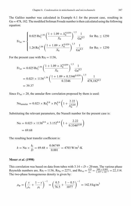
Kandlikar I044527-Ch06.tex 26/10/2005 18: 15 Page 387
Chapter 6. Condensation in minichannels and microchannels 387
The Galileo number was calculated in Example 6.1 for the present case, resulting inGa = 478, 182. The modified Soliman Froude number is then calculated using the followingequation:
Frso =
0.025 Re1.59l
(1 + 1.09 × X 0.039
tt
Xtt
)1.51
Ga0.5 for Rel ≤ 1250
1.26 Re1.04l
(1 + 1.09 × X 0.039
tt
Xtt
)1.51
Ga0.5 for Rel > 1250
For the present case with Rel = 1136,
Frso = 0.025 Re1.59l
(1 + 1.09 × X 0.039
tt
Xtt
)1.51
Ga0.5
= 0.025 × 11361.59(
1 + 1.09 × 0.33460.039
0.3346
)1.51
478,1820.5
= 39.37
Since Frso > 20, the annular flow correlation proposed by them is used:
Nuannular = 0.023 × Re0.8l × Pr0.4
l
(1 + 2.22
X 0.89tt
)
Substituting the relevant parameters, the Nusselt number for the present case is:
Nu = 0.023 × 11360.8 × 3.1520.4(
1 + 2.22
0.33460.89
)= 69.68
The resulting heat transfer coefficient is:
h = Nu × kl
D= 69.68 × 0.06749
0.001= 4703 W/m2-K
Moser et al. (1998)
This correlation was based on data from tubes with 3.14<D< 20 mm. The various phaseReynolds numbers are, Rel = 1136, Relo = 2271, and Revo = GD
µv= 300 × 0.001
1.357 × 10−5 = 22,114.The two-phase homogeneous density is given by:
ρtp =(
x
ρv+ 1 − x
ρl
)−1
=(
0.5
76.5+ 1 − 0.5
1077
)−1
= 142.8 kg/m3

Kandlikar I044527-Ch06.tex 26/10/2005 18: 15 Page 388
388 Heat transfer and fluid flow in minichannels and microchannels
The corresponding Froude and Weber numbers are:
Frtp = G2
gDρ2tp
= 3002
9.81 × 0.001 × 142.82 = 449.6
Wetp = G2D
σρtp= 3002 × 0.001
0.00427 × 142.8= 147.5
For the calculation of the equivalent Reynolds number, the required friction factors areobtained as follows:
flo = 0.079 × Re−0.25lo = 0.079 × 2271−0.25 = 0.01144
fvo = 0.079 × Re−0.25vo = 0.079 × 22114−0.25 = 0.006478
Constants required for the two-phase multiplier evaluation are calculated as follows:
A1 = (1 − x)2 +x2(ρl
ρv
)(fvo
flo
)= (1 − 0.5)2 +0.52
(1077
76.5
)(0.006478
0.01144
)=2.243
A2 = x0.78 (1 − x)0.24(ρl
ρv
)0.91 (µv
µl
)0.19 (1 − µv
µl
)0.70
= 0.50.78 (1 − 0.5)0.24(
1077
76.5
)0.91 (1.357 × 10⁻⁵
1.321 × 10⁻⁴
)0.19 (1 − 1.357 × 10⁻⁵
1.321 × 10⁻⁴
)0.70
= 3.293
Two-phase multiplier is obtained from the parameters calculated above:
φ2lo
= A1 + 3.24 × A2
Fr0.045tp × We0.035
tp= 2.243 + 3.24 × 3.293
449.60.045 × 147.50.035 = 3.008
The equivalent Reynolds Number is calculated in terms of this multiplier as follows:
Reeq = φ8/7lo × Relo = 3.0088/7 × 2271 = 7996
The Nusselt number is calculated in terms of this equivalent Reynolds number as follows:
Nu = 0.09940.126×Pr−0.448l × Re
−0.113×Pr−0.563l
l × Re1+0.11025×Pr−0.448
leq × Pr0.815
l(1.58 × ln Reeq − 3.28
) (2.58 × ln Reeq + 13.7 × Pr2/3
l − 19.1)
For the present case,
Nu = 0.09940.126×3.152−0.448×1136−0.113×3.152−0.563×79961+0.11025×3.152−0.448×3.1520.815
(1.58 × ln 7996 − 3.28)(2.58 × ln 7996 + 13.7 × 3.1522/3 − 19.1
)= 55.77

Kandlikar I044527-Ch06.tex 26/10/2005 18: 15 Page 389
Chapter 6. Condensation in minichannels and microchannels 389
Finally, the heat transfer coefficient is given by:
h = Nu × kl
D= 55.77 × 0.06749
0.001= 3764 W/m2-K
Chato (1962)
This model was proposed for stratified annular flow conditions when Rev < 35,000. Themodified latent heat of vaporization, which accounts for wall subcooling is given by:
h′lv = hlv ×
[1 + 0.68 × Cpl × (Tsat − Twall)
hlv
]
= 145,394 ×[
1 + 0.68 × 1611 × (55.21 − 52)
145,394
]= 148,910 J/kg
The heat transfer coefficient is obtained as follows:
h = 0.728 × Kc ×[
g × ρl × (ρl − ρv)× k3l × h′
lv
µl × (Tsat − Twall)× D
]1/4
With Kc = 0.76,
⇒ h = 0.728 × 0.76 ×[
9.81 × 1077 × (1077 − 76.5)× 0.067493 × 148910
1.321 × 10−4 × (55.21 − 52)× 0.001
]1/4
= 3216 W/m2-K
Boyko and Kruzhilin (1967)
This correlation relates the heat transfer coefficient in single-phase flow with the entire fluidflowing as a liquid to the two-phase heat transfer coefficient based on the mixture density,ρm = 142.8 kg/m3, calculated above. The bulk and wall Prandtl numbers are also required.Here the Prandtl number at the refrigerant pressure and wall temperature, Prw = 3.144.The single-phase heat transfer coefficient is calculated as follows:
h0 = 0.024 × kl
D×(
G × D
µl
)0.8
× Pr0.43l ×
(Prl
Prw
)0.25
For the present case,
h0 = 0.024 × 0.06749
0.001×(
300 × 0.001
1.321 × 10⁻⁴
)0.8
× 3.1520.43 ×(
3.152
3.144
)0.25
= 1286 W/m2-K
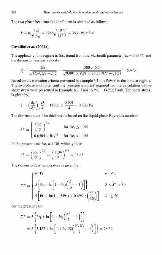
Kandlikar I044527-Ch06.tex 26/10/2005 18: 15 Page 390
390 Heat transfer and fluid flow in minichannels and microchannels
The two-phase heat transfer coefficient is obtained as follows:
h = h0
√ρl
ρm= 1286
√1077
142.8= 3531 W/m2-K
Cavallini et al. (2002a)
The applicable flow regime is first found from the Martinelli parameter Xtt = 0.3346, andthe dimensionless gas velocity:
j∗g = Gx√Dgρv(ρl − ρv)
= 300 × 0.5√0.001 × 9.81 × 76.5(1077 − 76.5)
= 5.473
Based on the transition criteria presented in example 6.1, the flow is in the annular regime.The two-phase multiplier and the pressure gradient required for the calculation of theshear stress were presented in Example 6.3. Thus, P/L = 14,500 Pa/m. The shear stress,is given by:
τ =(
dp
dz
)f
D
4= 14500 × 0.001
4= 3.625 Pa
The dimensionless film thickness is based on the liquid-phase Reynolds number:
δ+ =
(
Rel
2
)0.5
for Rel ≤ 1145
0.0504 × Re7/8l for Rel > 1145
In the present case Rel = 1136, which yields:
δ+ =(
Rel
2
)0.5
=(
1136
2
)0.5
= 23.83
The dimensionless temperature is given by:
T+ =
δ+ Prl δ+ ≤ 5
5{
Prl + ln[
1 + Prl
(δ+
5− 1
)]}5 < δ+ < 30
5[
Prl + ln(1 + 5 Prl)+ 0.495 ln(δ+
30
)]δ+ ≥ 30
For the present case,
T+ = 5{
Prl + ln[
1 + Prl
(δ+
5− 1
)]}
= 5{
3.152 + ln[
1 + 3.152(
23.83
5− 1
)]}= 28.54
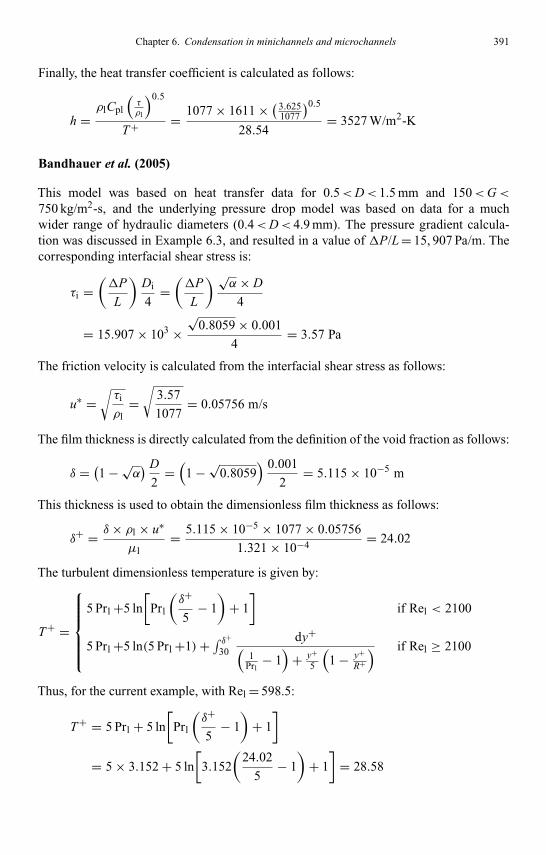
Kandlikar I044527-Ch06.tex 26/10/2005 18: 15 Page 391
Chapter 6. Condensation in minichannels and microchannels 391
Finally, the heat transfer coefficient is calculated as follows:
h =ρlCpl
(τρl
)0.5
T+ = 1077 × 1611 × ( 3.6251077
)0.528.54
= 3527 W/m2-K
Bandhauer et al. (2005)
This model was based on heat transfer data for 0.5<D< 1.5 mm and 150<G<
750 kg/m2-s, and the underlying pressure drop model was based on data for a muchwider range of hydraulic diameters (0.4<D< 4.9 mm). The pressure gradient calcula-tion was discussed in Example 6.3, and resulted in a value of P/L = 15, 907 Pa/m. Thecorresponding interfacial shear stress is:
τi =(P
L
)Di
4=(P
L
) √α× D
4
= 15.907 × 10³ ×√
0.8059 × 0.001
4= 3.57 Pa
The friction velocity is calculated from the interfacial shear stress as follows:
u∗ =√τi
ρl=√
3.57
1077= 0.05756 m/s
The film thickness is directly calculated from the definition of the void fraction as follows:
δ = (1 − √
α) D
2=(
1 − √0.8059
) 0.001
2= 5.115 × 10⁻⁵ m
This thickness is used to obtain the dimensionless film thickness as follows:
δ+ = δ× ρl × u∗
µl= 5.115 × 10−5 × 1077 × 0.05756
1.321 × 10−4 = 24.02
The turbulent dimensionless temperature is given by:
T+ =
5 Prl +5 ln[
Prl
(δ+
5− 1
)+ 1
]if Rel < 2100
5 Prl +5 ln(5 Prl +1)+ ∫ δ+30
dy+(1
Prl− 1
)+ y+
5
(1 − y+
R+) if Rel ≥ 2100
Thus, for the current example, with Rel = 598.5:
T+ = 5 Prl + 5 ln[
Prl
(δ+
5− 1
)+ 1
]
= 5 × 3.152 + 5 ln[
3.152(
24.02
5− 1
)+ 1
]= 28.58

Kandlikar I044527-Ch06.tex 26/10/2005 18: 15 Page 392
392 Heat transfer and fluid flow in minichannels and microchannels
Therefore, the heat transfer coefficient is:
h = ρl × Cpl × u∗
T+ = 1077 × 1611 × 0.05756
28.58= 3495 W/m2-K
The heat transfer coefficients predicted by the above models are depicted in the followinggraph.
5000
4000
3000
2000
1000
Hea
t tra
nsfe
r co
effic
ient
(W
/m2 -
K)
Chato
(196
2)
Boyko
and
Kru
zhilin
(196
7)
Solim
an e
t al. (
1968
)
Travis
s et a
l. (19
73)
Shan
(197
9)
Solim
an (1
986)
Dobso
n an
d Cha
to (1
998)
Mos
er e
t al. (
1998
)
Cavall
ini e
t al. (
2000
)
Bandh
auer
et a
l. (20
05)
0
It can be seen from this graph that there are considerable variations between the heattransfer coefficients predicted by these different models and correlations. One of the mainreasons for these variations is that most of these correlations have been applied in thiscase outside their ranges of applicability, either in the mass flux, the phase velocities, orparameters such as the Weber and Froude numbers as applicable. But the most importantreason for the differences is that all except the Bandhauer et al. (2005) model were basedprimarily on tube diameters in the ∼8 mm range, with a few correlations being proposedbased on limited data on ∼3 mm tubes. The channel under consideration in this exampleis a 1-mm channel.
6.7. Exercises
(1) Plot simulated air–water data points at different equally spaced combinations ofgas and liquid superficial velocities in the range 0.1–100 m/s, and 0.01–10.0 m/s,respectively, as is typically done in air–water studies. Now plot on the same graph,refrigerant R-134a (at 40◦C) points for the mass flux range 100–800 kg/m2-s in100 kg/m2-s increments and quality increments of 0.10; that is compute the vaporand liquid superficial velocities for these G, x combinations and plot on the air–water

Kandlikar I044527-Ch06.tex 26/10/2005 18: 15 Page 393
Chapter 6. Condensation in minichannels and microchannels 393
superficial velocity graph. Assume a 3 mm ID channel. Use this graph to com-ment on extending air–water flow regime maps to refrigerant condensation. Proposeappropriate means to transform air–water results to refrigerant predictions based oncomparisons of the relevant properties.
(2) Flow regime maps are often plotted on the basis of superficial velocities, in whichthe phases are assumed to occupy the entire channel cross section. While this is acommonly used practice out of convenience, what are the disadvantages of choosingsuperficial velocities instead of actual phase velocities? Quantify for a range of flowpatterns.
(3) Conduct a dimensional analysis to identify the dimensionless parameters that wouldquantify transitions between the four principal regimes: intermittent, wavy, annular,and mist flow, by considering viscous, surface tension, inertia, and gravity forces.Conduct parametric analyses to choose the most significant parameters across thescales.
(4) Estimate liquid film thickness as a function of three different void fraction modelsin annular flow, and its effect on the heat transfer coefficient. Refer to El Hajal(2003) and Thome (2003) for guidance. How would your conclusions change forintermittent or stratified flows?
(5) One of the uncertainties often overlooked in reporting pressure drop results inmicrochannels is the effect tolerances in tube diameter. Conduct a parametricanalysis of the change in pressure drop in a 1-mm channel during annular flowcondensation of refrigerant R-22 across the quality range 0.3< x< 0.8. Use a rea-sonable range of tolerances in the tube diameter to illustrate these effects. Use amass flux of 400 kg/m2-s, at a saturation temperature of 45◦C. Comment on howthis variation would change at evaporating conditions (e.g. 5◦C).
(6) Develop a quantitative indicator of momentum coupling of liquid and vapor phasesin condensing flows based on the papers of Lee and Lee (2001), the origin of the Ccoefficient expression developed by Chisholm (1967) for the Lockhart–Martinelli(1949) two-phase multiplier approach, and the discussions in the papers by Kawaharaet al. (2002) and Chung and Kawaji (2004). Estimate numerical values of thismeasure for 10 µm<Dh < 10 mm.
(7) Estimate the difference in saturation temperature decrease due to the flow of refrig-erant R-22 in a 0.5-mm channel at a mass flux of 200 kg/m2-s by computing thecondensation in 10% quality increments and accounting for frictional and deceler-ation contributions. Assume an appropriate bulk-wall temperature difference. Plotthe pressure drop in each increment, and the corresponding decrease in saturationtemperature. Use two different pressure drop models, one based on air–water studies,another based on refrigerant condensation.
(8) Microchannels are especially attractive due to the high heat transfer coefficients theyoffer. In measuring these heat transfer coefficients, one has to measure the heat trans-fer rate using, typically, a rise in coolant temperature, and a temperature differencebetween the refrigerant and the wall. Assume channel Dh = 0.5 mm. Assume furtherthat the heat transfer coefficient needs to be measured in increments of x = 0.10.First estimate the heat transfer rate to achieve this condensation at this mass flux.How accurately can this heat transfer rate be measured in a single microchannel?

Kandlikar I044527-Ch06.tex 26/10/2005 18: 15 Page 394
394 Heat transfer and fluid flow in minichannels and microchannels
What changes in coolant temperature would be required to effect this heat transferacross the test section? Is this realistic – estimate the uncertainties in heat transferrate measurement using reasonable thermocouple and mass flow rate measurementuncertainties. In an attempt to improve the uncertainties, multiple channels in par-allel are proposed. How many channels would be required to achieve accuratelymeasurable heat transfer rates? What are the drawbacks to using multiple channels.Next, estimate the heat transfer coefficient in condensing R-134a at 450 kg/m2-sand 50◦C using one of the available models. What refrigerant-wall temperature dif-ference would this cause in a channel that accomplishes the 10% quality change?(you will have to choose a reasonable test section length). How accurately can thistemperature difference be measured? What would be the resulting heat transfer coef-ficient uncertainty? How would the uncertainty vary with mass flux – quantify? Howwould the uncertainty change if R-134a is substituted with steam?
(9) It has been stated in this chapter that boundary-layer analyses in the liquid film andtwo-phase multiplier approaches are essentially equivalent methods of analyzingannular flow heat transfer. Refer to Dobson and Chato (1998) for background onthis matter. Conduct parallel derivations of these two approaches to point out theessential similarities. Also comment on any significant differences.
(10) Most heat transfer models recommend simply extending annular flow models to theintermittent flow. Develop a methodology for conducting this extension on a rationalbasis by accounting for the slug/bubble frequency.
(11) Will intermittent flow heat transfer coefficients be higher or lower than those inannular flow? Why? Will they be higher or lower than those in single-phase gas orsingle-phase liquid flow? Why? Demonstrate through approximate models, usingR-134a condensing at a 35◦C through a 200 µm channel at 100 kg/m2-s.
(12) Assuming that condensing flows would go through a progression of annular–mist-homogeneous flow as the reduced pressure is increased, identify the most importantfluid properties and the corresponding dimensionless parameters, and investigatechanges in these quantities as the pressure is increased from 0.2 × pr to 0.9 × pr .How would the pressure drop and heat transfer be affected in this progression?
(13) Design an R-22 condenser that transfers 3 kW at a saturation temperature of 55◦C,with the refrigerant entering as a saturated vapor and leaving as a saturated liquid.Dry air flowing in crossflow at 4.8E-01 m3/s, with an inlet temperature of 35◦C anda heat transfer coefficient of 50 W/m2-K is the cooling medium. Use copper tubingwith copper fins on the air side that yield a factor of 10 surface area enhancement.The efficiency of the fins can be assumed to be 90%. Choose the tubing size andwall thickness from standard tables such that the drop in refrigerant saturation tem-perature (due to the pressure drop) is less than 1.5◦C. Account for the flow regimevariation over the length of the heat exchanger. Choose quality and/or tube lengthincrements of reasonable size that demonstrate the flow phenomena and the heattransfer coefficient and pressure drop variations. Assume a horizontal orientation.
(14) Repeat problem 13 by changing the design to an optimal parallel-serpentine arrange-ment of extruded Aluminum tubes with twenty 0.7 mm microchannel tubes with thesame amount of air-side Aluminum fin surface area enhancement as in problem 13.Thus, decrease the number or tubes per pass as condensation proceeds so that a

Kandlikar I044527-Ch06.tex 26/10/2005 18: 15 Page 395
Chapter 6. Condensation in minichannels and microchannels 395
larger flow area is provided in the initial passes to account for the higher flow veloc-ities, and decrease the number of parallel tubes in subsequent passes. Compare thesizes (total material volume of each heat exchanger including tube and fin volume)resulting from these two approaches (Problems 13 and 14) and comment.
References
Akers, W. W., Deans, H. A., and Crosser, O. K., Condensation heat transfer within horizontal tubes,Chem. Eng. Prog. Symp. Series, 55(29), 171–176, 1959.
Akers, W. W. and Rosson, H. F., Condensation inside a horizontal tube, Chem. Eng. Prog. Symp.Series, 59, 145–149, 1960.
Ali, M. I., Sadatomi, M., and Kawaji, M., Adiabatic two-phase flow in narrow channels between twoflat plates, Can. J. Chem. Eng., 71(5), 657–666, 1993.
Alves, G. E., Cocurrent liquid–gas flow in a pipe-line contactor, Chem. Eng. Prog., 50(9): 449–456,1954.
Ananiev, E. P., Boyko, L. D., and Kruzhilin, G. N., Heat transfer in the presence of steam condensationin a horizontal tube, Proc. First Int. Heat Trans. Conf. Part II : 290, 1961.
Annunziato, M. and Girardi, G., Horizontal two phase flow: a statistical method for flow patternrecognition, Paper F1, 3rd Int. Conf. Multi-Phase Flow, The Hague, Netherlands, The Hague,Netherlands, 169–185, 1987.
Armand, A. A., The resistance during the movement of a two-phase system in horizontal pipes, Izv.Vses. Teplotekh. Inst., 1, 16–23 (AERE-Lib/Trans 828), 1946.
Azer, N. Z., Abis, L. V., and Soliman, H. M., Local heat transfer coefficients during annular flowcondensation, ASHRAE Transactions, 78 (Part 2), 135–143, 1972.
Bae, S., Maulbetsch, J. S., and Rohsenow, W. M., Refrigerant forced-convection condensation insidehorizontal tubes, 77 (Part 2), 104–113, 1971.
Baker, O., Simultaneous flow of oil and gas, Oil Gas J., 53, 185–195, 1954.Bandhauer, T. M., Agarwal, A., and Garimella, S., Measurement and modeling of condensation heat
transfer coefficients in circular microchannels, Proceedings of ICMM2005, The 3rd InternationalConference on Microchannels and Minichannels, June 13–15, 2005, ICMM2005- 75248, Toronto,Ontario, Canada, 2005.
Barajas, A. M. and Panton, R. L., The effects of contact angle on two-phase flow in capillary tubes,Int. J. Multiphase Flow, 19(2), 337–346, 1993.
Barnea, D., Luninski, Y., and Taitel, Y., Flow pattern in horizontal and vertical two phase flow insmall diameter tubes, Can. J. Chem. Eng., 61(5), 617–620, 1983.
Baroczy, C. J., Correlation of liquid fraction in two-phase flow with applications to liquid metals,Chem. Eng. Prog. Symp. Series, 61(57), 179–191, 1965.
Baroczy, C. J., Systematic correlation for two-phase pressure drop, Chem. Eng. Prog. Symp. Series,62(64), 232–249, 1966.
Baroczy, C. J. and Sanders, V. D., Pressure drop for flowing vapors condensing in straight horizontaltube, ASME Meeting WA-257, November 26–December 1 1961, American Society of MechanicalEngineers (ASME), New York, NY, USA, 16, 1961.
Beattie, D. R. H. and Whalley, P. B., A simple two-phase frictional pressure drop calculation method,Int. J. Multiphase Flow, 8(1), 83–87, 1982.
Blangetti, F. L. and Schlunder, E. U., Local heat transfer coefficients of condensation in a verticaltube, Proceedings of the Sixth International Heat Transfer Conference, 437–442, 1978.

Kandlikar I044527-Ch06.tex 26/10/2005 18: 15 Page 396
396 Heat transfer and fluid flow in minichannels and microchannels
Boyko, L. D. and Kruzhilin, G. N., Heat transfer and hydraulic resistance during condensation ofsteam in a horizontal tube and in a bundle of tubes, Int. J. Heat Mass Trans., 10(3), 361–373,1967.
Brauner, N. and Maron, D. M., Identification of the range of small diameters conduits, regardingtwo-phase flow pattern transitions, Int. Commun. Heat Mass Trans., 19(1), 29–39, 1992.
Breber, G., Palen, J. W., and Taborek, J., Prediction of horizontal tubeside condensation of pure com-ponents using flow regime criteria, Condens Heat Transfer, Presented at National Heat TransferConference, 18th, August 6–8 1979, 1–8, 1979.
Breber, G., Palen, J. W., and Taborek, J., Prediction of horizontal tubeside condensation of purecomponents using flow regime criteria, J. Heat Trans., Transac. ASME, 102(3), 471–476, 1980.
Butterworth, D., A comparison of some void-fraction relationships for co-current gas–liquid flow,Int. J. Multiphase Flow, 1(6), 845–850, 1975.
Cai, Y., Wambsganss, M. W., and Jendrzejczyk, J. A., Application of chaos theory in identificationof two-phase flow patterns and transitions in a small, horizontal, rectangular channel, J. Fluid.Eng., Trans. ASME, 118(2), 383–390, 1996.
Carey, V. P., Liquid–vapor Phase-change Phenomena: An Introduction to the Thermophysics ofVaporization and Condensation Processes in HeatTransfer Equipment. Washington, DC,Taylor &Francis Series, Hemisphere Pub. Corp, 1992.
Carnavos, T. C., Cooling air in turbulent flow with internally finned tubes, 1(2), 41–46, 1979.Carnavos, T. C., Heat transfer performance of internally finned tubes in turbulent flow, 1(4),
32–37, 1980.Carpenter, F. G. and Colburn, A. P., The effect of vapor velocity on condensation inside tubes,
General Discussion of Heat Transfer, The Institute of Mechanical Engineers and ASME, 20–26,1951.
Cavallini, A. and Zecchin, R., Dimensionless correlation for heat transfer in forced convectioncondensation, International Heat Transfer Conference, 5th, Proceeding, 309–313, 1974.
Cavallini, A., Del Col, D., Doretti, L., Longo, G. A., and Rossetto, L., Heat transfer and pressuredrop during condensation of refrigerants inside horizontal enhanced tubes: Transfert de chaleuret chute de pression lors de la condensation de frigorigenes a l’interieur de tubes horizontaux asurface augmentee, Int. J. Refrig., 23(1), 4–25, 2000.
Cavallini, A., Censi, G., Del Col, D., Doretti, L., Longo, G. A., and Rossetto, L., Experimentalinvestigation on condensation heat transfer and pressure drop of new HFC refrigerants (R134a,R125, R32, R410A, R236ea) in a horizontal smooth tube: [Etude experimentale sur le transfertde chaleur lors de la condensation et sur la chute de pression des nouveaux frigorigenes HFC(R134a, R125, R32, R410A, et R236ea) dans un tube lisse horizontal], Int. J. Refrig., 24(1),73–87, 2001.
Cavallini, A., Censi, G., Del Col, D., Doretti, L., Longo, G. A., and Rossetto, L., Condensation ofhalogenated refrigerants inside smooth tubes, HVAC and R Research, 8(4), 429–451, 2002a.
Cavallini, A., Censi, G., Del Col, D., Doretti, L., Longo, G. A., Rossetto, L., and Mathur, G. D.,In-tube condensation of halogenated refrigerants, 2002 ASHRAE Winter Meeting, January13–16 2002, Atlantic City, NJ, Amer. Soc. Heating, Ref. Air-Conditioning Eng. Inc.,146–161, 2002b.
Cavallini, A., Censi, G., Del Col, D., Doretti, L., Longo, G. A., Rossetto, L., and Zilio, C., Conden-sation inside and outside smooth and enhanced tubes – a review of recent research, Int. J. Refrig.,26(4), 373–392, 2003.
Cavallini, A., Del Col, D., Doretti, L., Matkovic, M., Rossetto, L., and Zilio, C., Condensation heattransfer and pressure gradient inside multiport minichannels, Heat Trans. Eng., 26(3), 45–55,2005.
Chaddock, J. B., Film condensation of vapor in horizontal tube, Refrig. Eng., 65(4), 36–41, 1957.

Kandlikar I044527-Ch06.tex 26/10/2005 18: 15 Page 397
Chapter 6. Condensation in minichannels and microchannels 397
Chato, J. C., Laminar condensation inside horizontal and inclined tubes, ASHRAE J., 4(2), 52–60,1962.
Chen, I. Y. and Kocamustafaogullari, G., Condensation heat transfer studies for stratified,cocurrent two-phase flow in horizontal tubes, Int. J. Heat Mass Trans., 30(6), 1133–1148,1987.
Chen, I. Y., Yang, K.-S., Chang, Y.-J., and Wang, C.-C., Two-phase pressure drop of air–water andR-410A in small horizontal tubes, Int. J. Multiphase Flow, 27(7), 1293–1299, 2001.
Chen, S. J., Reed, J. G., and Tien, C. L., Reflux condensation in a two-phase closed thermosyphon,Int. J. Heat Mass Trans., 27(9), 1587–1594, 1984.
Chen, S. L., Gerner, F. M., and Tien, C. L., General film condensation correlations, Exp. Heat Trans.,1(2), 93–107, 1987.
Chexal, B. and Lellouche, G. S., A full range drift-flux correlation for vertical flow, Electric PowerResearch Institute report EPRI-NP-3989-SR (revision 1), Palo Alto, CA, 1986.
Chexal, B., Lellouche, G. S., Horowitz, J., and Healzer, J., A void fraction correlation for generalizedapplications, Prog. Nucl. Energy, 27, 255–295, 1992.
Chexal, B., Merilo, M., Maulbetsch, J., Horowitz, J., Harrison, J., Westacott, J. C., Peterson, C.,Kastner, W., and Schmidt, H., Void fraction technology for design and analysis, Electric PowerResearch Institute. Palo Alto, CA, 1997.
Chisholm, D., A theoretical basis for the Lockhart–Martinelli correlation for two-phase flow, Int. J.Heat Mass Trans., 10(12), 1767–1778, 1967.
Chisholm, D., Pressure gradients due to friction during the flow of evaporating two-phase mixturesin smooth tubes and channels, Int. J. Heat Mass Trans., 16(2), 347–358, 1973.
Chisholm, D., Two-phase flow in pipelines and heat exchangers. London, New York: G. Godwin inassociation with the Institution of Chemical Engineers, 1983.
Chisholm, D. and Sutherland, L. A., Prediction of pressure gradients in pipeline systems duringtwo-phase flow, Proc. Instit. Mech. Eng., 24–32, 1969–70.
Chitti, M. S. and Anand, N. K., An analytical model for local heat transfer coefficients for forcedconvective condensation inside smooth horizontal tubes, Int. J. Heat MassTrans., 38(4), 615–627,1995.
Chitti, M. S. and Anand, N. K., Condensation heat transfer inside smooth horizontal tubes for R-22and R-32/125 mixture, HVAC&R Res., 2(1), 79–101, 1996.
Chun, K. R. and Seban, R. A. Heat transfer to evaporating liquid films, J. Heat Trans., 93 Ser C(4),391–396, 1971.
Chung, P. M.-Y. and Kawaji, M., The effect of channel diameter on adiabatic two-phase flowcharacteristics in microchannels, Int. J. Multiphase Flow, 30(7–8), 735–761, 2004.
Chung, P. M.-Y., Kawaji, M., Kawahara, A., and Shibata, Y., Two-phase flow through squareand circular microchannels – effects of channel geometry, J. Fluid. Eng., 126(4), 546–552,2004.
Churchill, S. W., Friction-factor equation spans all fluid-flow regimes, Chem. Eng. Prog., 84(24),91–92, 1977.
Churchill, S. W. and Usagi, R., A general expression for the correlation of rates of transfer and otherphenomena, AIChE J., 18(6), 1121–1128, 1972.
Cicchitti, A., Lombardi, C., Silvestri, M., Soldaini, G., and Zavattarelli, R., Two-phase coolingexperiments: pressure drop, heat transfer and burnout measurements, Energ. Nucl., 7(6), 407–425,1960.
Clarke, N. N. and Rezkallah, K. S., A study of drift velocity in bubbly two-phase flow undermicrogravity conditions, Int. J. Multiphase Flow, 27(9), 1533–1554, 2001.
Colebrook, C. F., Turbulent flow in pipes, with particular reference to the transition between thesmooth and rough pipe laws, J. Instit. Civil Eng., 11, 133–156, 1939.

Kandlikar I044527-Ch06.tex 26/10/2005 18: 15 Page 398
398 Heat transfer and fluid flow in minichannels and microchannels
Coleman, J. W. and Garimella, S., Characterization of two-phase flow patterns in small diameterround and rectangular tubes, Int. J. Heat Mass Trans., 42(15), 2869–2881., 1999.
Coleman, J. W. and Garimella, S., Two-phase flow regime transitions in microchannel tubes: theeffect of hydraulic diameter, Orlando, FL: American Society of Mechanical Engineers, HeatTransfer Division, 71–83, 2000a.
Coleman, J. W. and Garimella, S., Visualization of two-phase refrigerant flow during phase change,Proceedings of the 34th National Heat Transfer Conference, Pittsburgh, PA, ASME, 2000b.
Coleman, J. W. and Garimella, S., Two-phase flow regimes in round, square and rectangular tubesduring condensation of refrigerant R134a, Int. J. Refrig., 26(1), 117–128, 2003.
Collier, J. G. and Thome, J. R., Convective boiling and condensation, Oxford, New York: ClarendonPress, Oxford University Press, 1994.
Cornwell, K. and Kew, P. A., Boiling in small parallel channels, Energy Efficiency in ProcessTechnology, P. A. Pilavachi, New York: Elsevier, 624–638, 1993.
Damianides, C. A. and Westwater, J. W., Two-phase flow patterns in a compact heat exchanger andin small tubes, Second UK National Conference on Heat Transfer (2 Vols), Scotland: Glasgow,1257–1268, 1988.
Das, R. K. and Pattanayak, S., Electrical impedance method for flow regime identification in verticalupward gas–liquid two-phase flow, Measurem. Sci. Technol., 4(12), 1457–1463, 1993.
Das, R. and Pattanayak, S., Measurement of void fraction in different flow regimes of a verticalgas–liquid flow through narrow tubes, Measurem. Sci. Technol., 5(12), 1538–1545, 1994a.
Das, R. K. and Pattanayak, S., Bubble to slug flow transition in vertical upward two-phase flowthrough narrow tubes, Chem. Eng. Sci., 49(13), 2163–2172, 1994b.
Das, R. and Pattanayak, S., Bubble to slug flow transition in vertical upward two-phase flow ofcryogenic fluids, Cryogenics, 35(7), 421–426, 1995a.
Das, R. and Pattanayak, S., Flow regime identification in cryogenic gas–liquid flow through verticaltubes, Cryogenics, 35(6), 393–398, 1995b.
Das, R. and Pattanayak, S., Detection and analysis of transition from annular to intermittent flow invertical tubes, Can. J. Chem. Eng., 74(1), 49–57, 1996.
Dittus, W. and Boelter, L. M. K., Heat transfer in automobile radiators of the tubular type, Universityof California – Publications in Engineering, 2(13), 443–461, 1930.
Dobson, M. K., Heat transfer and flow regimes during condensation in horizontal tubes, PhD Thesis,Mechanical and Industrial Engineering, University of Illinois at Urbana-Champaign, Urbana-Champaign, IL, 1994.
Dobson, M. K. and Chato, J. C., Condensation in smooth horizontal tubes, J. Heat Trans., Transac.ASME, 120(1), 193–213, 1998.
Dobson, M. K., Chato, J. C., Hinde, D. K., and Wang, S. P., Experimental evaluation of internalcondensation of refrigerants R-12 and R-134a, Proceedings of the ASHRAE Winter Meet-ing, January 23–26 1994, New Orleans, LA, USA, ASHRAE, Atlanta, GA, USA, 744–754,1994.
Dukler, A. E., Fluid mechanics and heat transfer in vertical falling film systems, Chem. Eng. Prog.Symp. Series, 56(30), 1–10, 1960.
Dukler, A. E. and Hubbard, M. G., A model for gas–liquid slug flow in horizontal and near horizontaltubes, Ind. Eng. Chem. Fund., 14(4), 337–347, 1975.
Dukler, A. E., Wicks III, M., and Cleveland, R. G., Frictional pressure drop in two-phase flow, AIChEJ., 10(1), 38–51, 1964.
Eckels, S. J., Doerr, T. M., and Pate, M. B., In-tube heat transfer and pressure drop of R-134a andester lubricant mixtures in a smooth tube and a micro-fin tube: part I – evaporation, Proceedingsof the ASHRAE Annual Meeting, June 25–29 1994, Orlando, FL, USA, ASHRAE, Atlanta, GA,USA, 265–282, 1994.

Kandlikar I044527-Ch06.tex 26/10/2005 18: 15 Page 399
Chapter 6. Condensation in minichannels and microchannels 399
Ekberg, N. P., Ghiaasiaan, S. M., Abdel-Khalik, S. I., Yoda, M., and Jeter, S. M., Gas–liquidtwo-phase flow in narrow horizontal annuli, Nucl. Eng. Des., 192(1), 59–80, 1999.
El Hajal, J., Thome, J. R., and Cavallini, A., Condensation in horizontal tubes, part 1: two-phaseflow pattern map, Int. J. Heat Mass Trans., 46(18), 3349–3363, 2003.
Elkow, K. J. and Rezkallah, K. S., Statistical analysis of void fluctuations in gas–liquid flows under1 – g and µ – g conditions using a capacitance sensor, Int. J. Multiphase Flow, 23(5), 831–844,1997a.
Elkow, K. J. and Rezkallah, K. S., Void fraction measurements in gas–liquid flows under 1 – g andµ – g conditions using capacitance sensors, Int. J. Multiphase Flow, 23(5), 815–829, 1997.
Feng, Z. and Serizawa, A., Visualization of two-phase flow patterns in an ultra-small tube,Proceedings of the 18th Multiphase Flow Symposium of Japan, Suita, Osaka, Japan, 33–36,1999.
Feng, Z. and Serizawa, A., Measurement of steam–water bubbly flow in ultra-small capillary tube,Proceedings of the 37th National Heat Transfer Symposium of Japan, 351–352, 2000.
Friedel, L., Improved friction pressure drop correlations for horizontal and vertical two phase pipeflow, European Two Phase Flow Group Meeting, Ispra, Italy, paper E2, 1979.
Friedel, L., Pressure drop during gas/vapor–liquid flow in pipes, Int. Chem. Eng., 20(3), 352–367,1980.
Fukano, T. and Kariyasaki, A., Characteristics of gas–liquid two-phase flow in a capillary tube, Nucl.Eng. Des., 141(1–2), 59–68, 1993.
Fukano, T., Kariyasaki, A., and Kagawa, M., Flow patterns and pressure drop in isothermal gas–liquid concurrent flow in a horizontal capillary tube, Proceedings of the 1989 ANS National HeatTransfer Conference, Philadelphia, 153–161, 1989.
Galbiati, L. andAndreini, P., Flow pattern transition for vertical downward two-phase flow in capillarytubes. Inlet mixing effects, Int. Commun. Heat Mass Trans., 19(6), 791–799, 1992a.
Galbiati, L. and Andreini, P., The transition between stratified and annular regimes for horizon-tal two-phase flow in small diameter tubes, Int. Commun. Heat Mass Trans., 19(2), 185–190,1992b.
Galbiati, L. and Andreini, P. Flow pattern transition for horizontal air–water flow in capillary tubes.A microgravity equivalent system simulation, Int. Commun. Heat Mass Trans., 21(4), 461–468,1994.
Garimella, S., Condensation flow mechanisms in microchannels: basis for pressure drop and heattransfer models, Heat Trans. Eng., 25(3), 104–116, 2004.
Garimella, S., Condensation flow mechanisms, pressure drop and heat transfer in microchannels.Microscale HeatTransfer- Fundamental andApplications, S. Kakac, L. L.Vasiliev,Y. Bayazitoglu,Y. Yener eds., The Netherlands: Kluwer Academic Publishers, 2005.
Garimella, S., Agarwal, A., and Killion, J. D., Condensation pressure drop in circular microchannels,Heat Trans. Eng., 26(3), 1–8, 2005.
Garimella, S. V. and Singhal, V., Single-phase flow and heat transport and pumping considerationsin microchannel heat sinks, Heat Trans. Eng., 25(1), 15–25, 2004.
Garimella, S. V. and Sobhan, C. B., Transport in microchannels – a critical review. Ann. Rev. HeatTrans., 13, 2003.
Garimella, S. and Wicht, A., Air-cooled condensation of ammonia in flat-tube, multi-louver fin heatexchangers, Proceedings of the 1995 ASME International Mechanical Engineering Congressand Exposition, November 12–17 1995, San Francisco, CA, ASME, New York, NY, 47–58,1995.
Garimella, S. and Bandhauer, T. M., Measurement of condensation heat transfer coefficients inmicrochannel tubes, 2001ASME International Mechanical Engineering Congress and Exposition,New York, NY, American Society of Mechanical Engineers, 243–249, 2001.

Kandlikar I044527-Ch06.tex 26/10/2005 18: 15 Page 400
400 Heat transfer and fluid flow in minichannels and microchannels
Garimella, S., Killion, J. D., and Coleman, J. W., An experimentally validated model for two-phasepressure drop in the intermittent flow regime for circular microchannels, J. Fluid. Eng., 124(1),205–214, 2002.
Garimella, S., Agarwal, A., and Coleman, J. W., Two-phase pressure drops in the annular flowregime in circular microchannels, 21st IIR International Congress of Refrigeration, Washington,DC, International Institute of Refrigeration, 2003a.
Garimella, S., Killion, J. D., and Coleman, J. W., An experimentally validated model for two-phasepressure drop in the intermittent flow regime for noncircular microchannels, J. Fluid. Eng., 125(5),887–894, 2003b.
Geraets, J. J. M. and Borst, J. C., A capacitance sensor for two-phase void fraction measurement andflow pattern identification, Int. J. Multiphase Flow, 14(3), 305–320, 1988.
Gibson, A. H., On the motion of long air-bubbles in a vertical tube, Phil. Mag., 26, 952–965, 1913.Gnielinski, V., New equations for heat and mass transfer in turbulent pipe and channel flow, Int.
Chem. Eng., 16(2), 359–368, 1976.Goto, M., Inoue, N., and Ishiwatari, N., Condensation and evaporation heat transfer of R410A inside
internally grooved horizontal tubes, Int. J. Refrig., 24(7), 628–638, 2001.Goto, M., Inoue, N., and Yonemoto, R., Condensation heat transfer of R410A inside internally
grooved horizontal tubes, Int. J. Refrig., 26(4), 410–416, 2003.Govier, G. W. and Omer, M. M., The horizontal pipeline flow of air–water mixtures, Cana. J. Chem.
Eng., 93–104, 1962.Govier, G. W. and Short, W. L., The upward vertical flow of air–water mixtures, Can. J. Chem. Eng.,
195–202, 1958.Govier, G. W., Radford, B. A., and Dunn, J. S. C., The upward vertical flow of air water mixtures.
Part 1: effect of air and water rates on flow pattern, hold-up and pressure drop, Can. J. Chem.Eng., 35, 58–70, 1957.
Graham, D., Chato, J. C., and Newell, T. A., Heat transfer and pressure drop during condensation ofrefrigerant 134a in an axially grooved tube, Int. J. Heat Mass Trans., 42(11), 1935–1944, 1999.
Gregorig, R., Verfahrenstechnisch gunstigere fuhrung der mittel der Warmeubertragung beimverdampfen und kondensieren, Int. J. Heat Mass Trans., 5(3–4), 175–188, 1962.
Griffith, P. and Lee, K. S., Stability of annulus of liquid in tube, Transac. ASME, J. Basic Eng., 86(4),666–668, 1964.
Guo, Z., Condensation of R-410a in horizontal rectangular channel, PhD thesis, MechanicalEngineering, Texas A&M University, College Station, TX, 1998.
Guo, Z. and Anand, N. K., Analytical model to predict condensation of R-410A in a horizontalrectangular channel, J. Heat Trans. Transac. ASME, 122(3), 613–620, 2000.
Haraguchi, H., Koyama, S., and Fujii, T., Condensation of refrigerants HCFC22, HFC134a andHCFC123 in a horizontal smooth tube (1st report, proposal of empirical expressions for the localfrictional pressure drop), Transac. JSME (B), 60(574), 239–244, 1994a.
Haraguchi, H., Koyama, S., and Fujii, T., Condensation of refrigerants HCFC22, HFC134a andHCFC123 in a horizontal smooth tube (2nd report, proposal of empirical expressions for thelocal heat transfer coefficient), Transac. JSME (B), 60(574), 245–252, 1994b.
Hashizume, K., Flow pattern, void fraction and pressure drop of refrigerant two-phase flow in ahorizontal pipe–I. Experimental data, Int. J. Multiphase Flow, 9(4), 399–410, 1983.
Hashizume, K. and Ogawa, N., Flow pattern, void fraction and pressure drop of refrigerant two-phase flow in a horizontal pipe–III: comparison of the analysis with existing pressure drop dataon air/water and steam/water systems, Int. J. Multiphase Flow, 13(2), 261–267, 1987.
Hashizume, K., Ogiwara, H., and Taniguchi, H., Flow pattern, void fraction and pressure dropof refrigerant two-phase flow in a horizontal pipe–II: analysis of frictional pressure drop, Int. J.Multiphase Flow, 11(5), 643–658, 1985.

Kandlikar I044527-Ch06.tex 26/10/2005 18: 15 Page 401
Chapter 6. Condensation in minichannels and microchannels 401
Hetsroni, G., Handbook of Multiphase Systems, New York: Hemisphere, 1982.Hewitt, G. F. and Roberts, D. N., Studies of Two-Phase Flow Patterns by Simultaneous X-Ray
and Flash Photography, AERE-M 2159, London, UK: Her Majesty’s Stationery Office, 1969.Hewitt, G. F., Shires, G. L., and Bott, T. R., Process Heat Transfer. Boca Raton: CRC Press; Begell
House, 1994.Hibiki, T. and Mishima, K., Approximate method for measurement of phase-distribution in mul-
tiphase materials with small neutrondashattenuation using a neutron beam as a probe, Nucl.Instrum. Meth. in Phys. Res. Sec. A: Acceler., Spectr., Detect. Assoc. Equip., 374(3), 345–351,1996.
Hibiki, T. and Mishima, K., Flow regime transition criteria for upward two-phase flow in verticalnarrow rectangular channels, Nucl. Eng. Des., 203(2–3), 117–131, 2001.
Hibiki, T., Mishima, K., and Nishihara, H., Measurement of radial void fraction distribution oftwo-phase flow in a metallic round tube using neutrons as microscopic probes, Nucl. Instrum.Meth. Phys. Res. Sec. A: Acceler., Spectr., Detec. Assoc. Equip., 399(2–3), 432–438, 1997.
Hosler, E. R., Flow patterns in high pressure two-phase (steam–water) flow with heat addition, AIChESymposium Series, 54–66, 1968.
Hughmark, G. A., Holdup in gas–liquid flow, Chem. Eng. Prog., 58(4), 62–65, 1962.Hurlburt, E. T. and Newell, T. A., Characteristics of refrigerant film thickness, pressure drop, and
condensation heat transfer in annular flow, HVAC&R Res., 5(3), 229–248, 1999.Ide, H., Matsumura, H., and Fukano, T., Velocity characteristics of liquid lumps and its relation to
flow patterns in gas–liquid two-phase flow in vertical capillary tubes, Proceedings of the 1995ASME/JSME Fluids Engineering and Laser Anemometry Conference and Exhibition, August13–18 1995, Hilton Head, SC, USA, ASME, New York, NY, USA, 1–8, 1995.
Ide, H., Matsumura, H., Tanaka, Y., and Fukano, T., Flow patterns and frictional pressure drop ingas–liquid two-phase flow in vertical capillary channels with rectangular cross section, NipponKikai Gakkai Ronbunshu, B Hen/Trans. JSME, Part B, 63(606), 452–460, 1997.
Infante Ferreira, C. A., Newell, T. A., Chato, J. C., and Nan, X., R404A condensing under forcedflow conditions inside smooth, microfin and cross-hatched horizontal tubes, Int. J. Refrig., 26(4),433–441, 2003.
Isbin, H. S., Sher, N. C., and Eddy, K. C., Void fractions in two-phase steam–water flow, AIChE J.,3(1), 136–142, 1957.
Ishii, M., One-dimensional drift-flux model and constitutive equations for between phases in varioustwo-phase flow regimes, ANL Report ANL-77-47, 1977.
Jaster, H. and Kosky, P. G., Condensation heat transfer in a mixed flow regime, Int. J. Heat MassTrans., 19(1), 95–99, 1976.
Jenkins, R., Two-phase two-component flow of water and air, MS, University of Delaware, 1947.Jiang,Y. and Garimella, S., Compact air-coupled and hydronically coupled microchannel heat pumps,
2001 ASME International Mechanical Engineering Congress and Exposition, November 11–162001, New York, NY, USA, American Society of Mechanical Engineers, 227–239, 2001.
Jones Jr., O. C. and Zuber, N., The interrelation between void fraction fluctuations and flow patternsin two-phase flow, Int. J. Multiphase Flow, 2(3), 273–306, 1975.
Jung, D. S. and Radermacher, R., Prediction of pressure drop during horizontal annular flow boilingof pure and mixed refrigerants, Int. J. Heat Mass Trans., 32(12), 2435–2446, 1989.
Kariyasaki, A., Fukano, T., Ousaka, A., and Kagawa, M., Characteristics of time-varying voidfraction in isothermal air–water cocurrent flow in horizontal capillary tube, Transac. JSME,57(B)(544), 4036–4043, 1991.
Kariyasaki, A., Fukano, T., Ousaka, A., and Kagawa, M., Isothermal air–water two-phase up anddownward flows in a vertical capillary tube (lst report, flow pattern and void fraction). Trans.JSME (Ser. B), 58, 2684–2690, 1992.

Kandlikar I044527-Ch06.tex 26/10/2005 18: 15 Page 402
402 Heat transfer and fluid flow in minichannels and microchannels
Kattan, N., Thome, J. R., and Favrat, D., Flow boiling in horizontal tubes: part 1 – development of adiabatic two-phase flow pattern map, J. Heat Trans. Transac. ASME, 120(1), 140–147, 1998a.
Kattan, N., Thome, J. R., and Favrat, D., Flow boiling in horizontal tubes: part 2 – new heat transferdata for five refrigerants, J. Heat Trans. Transac. ASME, 120(1), 148–155, 1998b.
Kattan, N., Thome, J. R., and Favrat, D., Flow boiling in horizontal tubes: part 3 – development ofa new heat transfer model based on flow pattern, J. Heat Trans., Transac. ASME, 120(1), 156–165,1998c.
Kawahara, A., Chung, P. M.-Y, and Kawaji, M., Investigation of two-phase flow pattern, void fractionand pressure drop in a microchannel, Int. J. Multiphase Flow, 28(9), 1411–1435, 2002.
Kawahara, A., Sadatomi, M., Okayama, K., Kawaji, M., and Chung, P. M.-Y., Effects of channeldiameter and liquid properties on void fraction in adiabatic two-phase flow through microchannels,Heat Trans. Eng., 26(3), 13–19, 2005.
Keska, J. K., Fernando, R. D., and Hamer, M.T., Experimental investigation of average parameters forair–water two-phase flow in a horizontal channel based on in-situ measurements, 28th NationalHeat Transfer Conference and Exhibition, August 9–12 1992, San Diego, CA, USA, Publ byASME, New York, NY, USA, 7–18, 1992.
Kew, P.A. and Cornwell, K., Correlations for the prediction of boiling heat transfer in small-diameterchannels, Appl. Therm. Eng., 17(8–10), 705–715, 1997.
Kim, N.-H., Cho, J.-P., Kim, J.-O., and Youn, B., Condensation heat transfer of R-22 and R-410Ain flat aluminum multi-channel tubes with or without micro-fins, Int. J. Refrig., 26(7), 830–839,2003.
Kolb, W. B. and Cerro, R. L., Coating the inside of a capillary of square cross section, Chem. Eng.Sci., 46(9), 2181–2195, 1991.
Kolb, W. B. and Cerro, R. L., Film flow in the space between a circular bubble and a square tube,J. Colloid Interf. Sci., 159(2), 302–311, 1993.
Kosky, P. G., Thin liquid films under simultaneous shear and gravity forces, Int. J. Heat Mass Trans.,14(8), 1220–1224, 1971.
Kosky, P. G. and Staub, F. W., Local condensing heat transfer coefficients in the annular flow regime,AIChE J., 17(5), 1037–1043, 1971.
Koyama, S. and Yu, J., Condensation heat transfer of pure refrigerant inside an internally groovedhorizontal tube, Proceedings of the JAR Annual Conference, 173–176, 1996.
Koyama, S., Kuwahara, K., and Nakashita, K., Condensation of refrigerant in a multi-port chan-nel, First International Conference on Microchannels and Minichannels, April 24–25 2003,Rochester, NY, USA, American Society of Mechanical Engineers, 193–205, 2003a.
Koyama, S., Kuwahara, K., Nakashita, K., and Yamamoto, K., An experimental study on condensa-tion of refrigerant R134a in multi-port extruded tube, Int. J. Refrig., 26(4), 425–432, 2003b.
Koyama, S., Lee, J., and Yonemoto, R., An investigation on void fraction of vapor–liquid two-phaseflow for smooth and microfin tubes with R134a at adiabatic condition, Int. J. Multiphase Flow,30(3), 291–310, 2004.
Kureta, M., Kobayashi, T., Mishima, K., and Nishihara, H., Pressure drop and heat transfer forflow-boiling of water in small-diameter tubes, JSME Int. J., Series B, 41(4), 871–879, 1998.
Kureta, M., Akimoto, H., Hibiki, T., and Mishima, K., Void fraction measurement in subcooled-boiling flow using high-frame-rate neutron radiography, Nucl. Technol., 136(2), 241–254, 2001.
Kureta, M., Hibiki, T., Mishima, K., and Akimoto, H., Study on point of net vapor generationby neutron radiography in subcooled boiling flow along narrow rectangular channels with shortheated length, Int. J. Heat Mass Trans., 46(7), 1171–1181, 2003.
Kutateladze, S. S., Fundamentals of Heat Transfer, New York: Academic Press, 1963.Lee, H. J. and Lee, S.Y., Pressure drop correlations for two-phase flow within horizontal rectangular
channels with small heights, Int. J. Multiphase Flow, 27(5), 783–796, 2001.

Kandlikar I044527-Ch06.tex 26/10/2005 18: 15 Page 403
Chapter 6. Condensation in minichannels and microchannels 403
Lin, S., Kwok, C. C. K., Li, R.-Y., Chen, Z.-H., and Chen, Z.-Y., Local frictional pressure drop duringvaporization of R-12 through capillary tubes, Int. J. Multiphase Flow, 17(1), 95–102, 1991.
Liu, D. and Garimella, S. V., Investigation of liquid flow in microchannels, J. Thermophys. HeatTrans., 18(1), 65–72, 2004.
Lockhart, R. W. and Martinelli, R. C., Proposed correlation of data for isothermal two-phase,two-component flow in pipes, Chem. Eng. Prog., 45(1), 39–45, 1949.
Lowe, D. C. and Rezkallah, K. S., Flow regime identification in microgravity two-phase flows usingvoid fraction signals Int. J. Multiphase Flow, 25(3), 433–457, 1999.
Lowry, B. and Kawaji, M., Adiabatic vertical two-phase flow in narrow flow channels, HeatTransfer – Houston 1988, Papers Presented at the 25th National Heat Transfer Conference,Houston, TX, AIChE, New York, NY, 133–139, 1988.
Mandhane, J. M., Gregory, G. A., and Aziz, K., A flow pattern map for gas–liquid flow in horizontalpipes, Int. J. Multiphase Flow, 1(4), 537–553, 1974.
Matuszkiewicz, A., Flamand, J. C., and Boure, J. A., The bubble–slug flow pattern transition andinstabilities of void fraction waves, Int. J. Multiphase Flow, 13(2), 199–217, 1987.
McAdams, W. H., Heat Transmission, New York: McGraw-Hill, 1954.Mikheev, M. A., Heat Transfer Fundamentals, Moscow: Gosenergoizdat, 1956.Miropolsky, Z. L., Heat transfer during condensation of high pressure steam inside a tube,
Teploenergetika, 3, 79–83, 1962.Mishima, K. and Hibiki, T., Some characteristics of air–water two-phase flow in small diameter
vertical tubes, Int. J. Multiphase Flow, 22(4), 703–712, 1996.Mishima, K. and Ishii, M., Flow regime transition criteria for upward two-phase flow in vertical
tubes, Int. J. Heat Mass Trans, 27(5), 723–737, 1984.Mishima, K. and Hibiki, T., Development of high-frame-rate neutron radiography and quantita-
tive measurement method for multiphase flow research, Nucl. Eng. Des., 184(2–3), 183–201,1998.
Mishima, K., Hibiki, T., and Nishihara, H., Some characteristics of gas–liquid flow in narrow rectan-gular ducts, International Journal of Multiphase Flow International Conference on MultiphaseFlows 91 – Tsukuba (ICM’91), September 23–27 1991, 19(1), 115–124, 1993.
Mishima, K., Hibiki, T., and Nishihara, H., Visualization and measurement of two-phase flow byusing neutron radiography, Nucl. Eng. Des., 175(1–2), 25–35, 1997.
Moore, A. E. and Turley, D. N., Two phase flow information from simple, rapid response timeinstruments, Papers Presented at the International Conference on the Physical Modelling ofMulti-Phase Flow, April 19–21 1983, Coventry, UK, BHRA, 353–376, 1983.
Moriyama, K., Inoue, A., and Ohira, H., Thermohydraulic characteristics of two-phase flow inextremely narrow channels (the frictional pressure drop and heat transfer of boiling two-phaseflow, analytical model), Heat Trans. – Jap. Res., 21(8), 838–856, 1992a.
Moriyama, K., Inoue, A., and Ohira, H., Thermohydraulic characteristics of two-phase flowin extremely narrow channels (the frictional pressure drop and void fraction of adiabatictwo-component two-phase flow), Heat Trans. – Jap. Res., 21(8), 823–837, 1992b.
Moser, K. W., Webb, R. L., and Na, B., A new equivalent Reynolds number model for condensationin smooth tubes, Transac. ASME, J. Heat Trans., 120(2), 410–417, 1998.
Muller-Steinhagen, H. and Heck, K., A simple friction pressure drop correlation for two-phase flowin pipes, Chem. Eng. Proces., 20(6), 297–308, 1986.
Nicholson, M. K., Aziz, K., and Gregory, G. A., Intermittent two phase flow in horizontal pipes:predictive models., 56(6), 653–663, 1978.
Nitheanandan, T., Soliman, H. M., and Chant, R. E., A proposed approach for correlating heattransfer during condensation inside tubes, ASHRAE Trans. (1990 Winter Meeting, Atlanta, GA),96(1), 230–241, 1990.

Kandlikar I044527-Ch06.tex 26/10/2005 18: 15 Page 404
404 Heat transfer and fluid flow in minichannels and microchannels
Nusselt, W., Die Oberflachen Kondensation des Wasserdampfes, Zeit. Ver. Deut. Ing., 60(27, 28),541–546, 569–575, 1916.
Owens, W. L., Two-phase pressure gradient, International Development in Heat Transfer, Part II.New York: ASME, 1961.
Palen, J. W., Breber, G., and Taborek, J., Prediction of flow regimes in horizontal tubeside condensa-tion, Proceedings of the 17th National Heat Transfer Conference, Salt Lake City, UT, Salt LakeCity, AIChE Paper No. 5, 1977.
Palm, B., Heat transfer in microchannels, Microscale Thermophys. Eng., 5(3), 155–175, 2001.Petukhov, B. S., Heat transfer and friction in turbulent pipe flow with variable physical properties,
Adv. Heat Trans., 6, 503–564, 1970.Premoli, A., Francesco, D., and Prina, A., A dimensionless correlation for determining the density
of two-phase mixtures, La Termotecnica, 25, 17–26, 1971.Rabas, T. J. and Arman, B., Effect of the exit condition on the performance of in-tube condensers,
Heat Trans. Eng., 21(1), 4–14, 2000.Rezkallah, K. S., Recent progress in the studies of two-phase flow at microgravity conditions, Adv.
Space Res., 16(7), 123–132, 1995.Rezkallah, K. S., Weber number based flow-pattern maps for liquid–gas flows at microgravity, Int.
J. Multiphase Flow, 22(6), 1265–1270, 1996.Rezkallah, K. S. and Zhao, L., A flow pattern map for two-phase liquid–gas flows under reduced
gravity conditions, Adv. Space Res., 16(7), 133–136, 1995.Rice, C. K., Effect of void fraction correlation and heat flux assumption on refrigerant charge inven-
tory predictions, ASHRAE Transactions: Technical and Symposium Papers Presented at the 1987Winter Meeting., New York, NY, ASHRAE, Atlanta, GA, 341–367, 1987.
Richardson, B. L., Some problems in horizontal two-phase two-component flow, PhD Thesis,Mechanical Engineering, Purdue University, West Lafayette.
Rohsenow, W. M., Heat transfer and temperature distribution in laminar–film condensation, Am. Soc.Mech. Eng. – Transac., 78(8), 1645–1648, 1956.
Rohsenow, W. M., Webber, J. H., and Ling, A. T., Effect of vapor velocity on laminarand turbulent–film condensation, Am. Soc. Mech. Eng. – Transac., 78(8), 1637–1642,1956.
Rohsenow, W. M., Webber, J. H., and Ling, A. T., Effect of vapor velocity on laminar andturbulent–film condensation, Am. Soc. Mech. Eng. – Transac., 78(8), 1637–1642, 1957.
Rosson, H. F. and Myers, J. A., Point values of condensing film coefficients inside horizontal pipe,Chem. Eng. Prog. Symp. Series, 61(59), 190–199, 1965.
Rouhani, S. Z. and Axelsson, E., Calculation of void volume fraction in the subcooled and qualityboiling regions, Int. J. Heat Mass Trans., 13(2), 383–393, 1970.
Rouhani, S. Z. and Becker, K. M., Measurements of void fraction for flow boiling of heavy water invertical round duct, Aktebolaget Atomenergies Rep. AE-106, 1963.
Rufer, C. E. and Kezios, S. P., Analysis of two-phase, one-component stratified flow withcondensation, Am. Soc. Mech. Eng. – Transac. – J. Heat Trans., 88(3), 265–275, 1966.
Sacks, P. S., Measured characteristics of adiabatic and condensing single-component two-phaseflow of refrigerant in a 0.377-in. diameter horizontal tube, Proceedings of the American Societyof Mechanical Engineers Winter Annual Meeting, 75-WA/HT-24, ASME, 12, 1975.
Sadatomi, M., Sato, Y., and Saruwatari, S., Two-phase flow in vertical noncircular channels, Int. J.Multiphase Flow, 8(6), 641–655, 1982.
Sardesai, R. G., Owen, R. G., and Pulling, D. J., Flow regimes for condensation of a vapour insidea horizontal tube, Chem. Eng. Sci., 36(7), 1173–1180, 1981.
Schlichting, H. and Gersten, K., Laminar–turbulent transition, Boundary Layer Theory, Springer:415–490, 2000.

Kandlikar I044527-Ch06.tex 26/10/2005 18: 15 Page 405
Chapter 6. Condensation in minichannels and microchannels 405
Serizawa, A. and Feng, Z., Two-phase flow in micro-channels, Proceedings of the 4th InternationalConference on Multiphase Flow, New Orleans, LA, 2001.
Serizawa, A. and Feng, Z., Two-phase fluid flow, Heat Transfer and Fluid Flow in Microchannels,G. P. Celata ed., New York, NY: Begell House, 1, 91–117, 2004.
Serizawa, A. and Kawara, Z., Two-phase flow in micro-channels, Proceedings of the 39th EuropeanTwo-Phase Flow Group Meeting, Averio, Portugal, 2001.
Serizawa, A., Feng, Z., and Kawara, Z., Two-phase flow in microchannels, Exp. Therm. Fluid Sci.,26(6–7), 703–714, 2002.
Shah, M. M., New correlation for heat transfer during boiling flow through pipes, Proc. Annu. Meet,June 27–July 1 1976, 82(part)2, 66–86, 1976.
Shah, M. M., A general correlation for heat transfer during film condensation inside pipes, Int.J. Heat Mass Trans., 22(4), 547–556, 1979.
Shin, J. S. and Kim, M. H., An experimental study of flow condensation heat transfer inside circularand rectangular mini-channels, Heat Trans. Eng., 26(3), 36–44, 2005.
Singh, A., Ohadi, M. M., and Dessiatoun, S. V., Empirical modeling of stratified–wavy flowcondensation heat transfer in smooth horizontal tubes, ASHRAETransac., 102(2), 596–603, 1996.
Smith, S. L., Void fractions in two- phase flow: a correlation based upon an equal velocity head model,Proceedings of the Institution of Mechanical Engineers, Thermodynamics and Fluid MechanicsGroup, 647–657, 1969.
Sobhan, C. B. and Garimella, S. V., A comparative analysis of studies on heat transfer and fluid flowin microchannels, Micros. Thermophys. Eng., 5(4), 293–311, 2001.
Soliman, H. M., On the annular-to-wavy flow pattern transition during condensation inside horizontaltubes, Can. J. Chem. Eng., 60(4), 475–481, 1982.
Soliman, H. M., Correlation of mist-to-annular transition during condensation, Can. J. Chem. Eng.,61(2), 178–182, 1983.
Soliman, H. M., Mist–annular transition during condensation and its influence on the heat transfermechanism, Int. J. Multiphase Flow, 12(2), 277–288, 1986.
Soliman, H. M., Schuster, J. R., and Berenson, P. J., A general heat transfer correlation for annularflow condensation, J. Heat Trans., 90, 267–276, 1968.
Souza, A. L., Chato, J. C., Wattelet, J. P., and Christoffersen, B. R., Pressure drop during two-phaseflow of pure refrigerants and refrigerant-oil mixtures in horizontal smooth tubes, 29th NationalHeat Transfer Conference, August 8–11 1993, Atlanta, GA, ASME, New York, NY, 35–41, 1993.
Souza, D. A. L. and Pimenta, M. D. M., Prediction of pressure drop during horizontal two-phase flowof pure and mixed refrigerants, Proceedings of the 1995 ASME/JSME Fluids Engineering andLaser Anemometry Conference and Exhibition, August 13–18 1995, Hilton Head, SC, ASME,New York, NY, 161–171, 1995.
Steiner, D., Heat transfer to boiling saturated liquids. VDI-Wär meatlas (VDI Heat Atlas).Düsseldorf, VDI-Gessellschaft Verfahrenstechnik und Chemieingenieurwesen (GCV), (Trans-lator: J.W. Fullarton), 1993.
Sugawara, S., Katsuta, K., lshihara, I., and Muto, T., Consideration on the pressure loss of two-phaseflow in small-diameter tubes, Proceeding 4th National Heat Transfer Symposium of Japan (inJapanese), 169–172, 1967.
Suo, M. and Griffith, P., Two-phase flow in capillary tubes, J. Basic Eng., 86, 576–582, 1964.Tabatabai, A. and Faghri, A., A new two-phase flow map and transition boundary accounting for sur-
face tension effects in horizontal miniature and micro tubes, J. HeatTrans., 123(5), 958–968, 2001.Taitel, Y. and Dukler, A. E., A model for predicting flow regime transitions in horizontal and near
horizontal gas–liquid flow, AIChE J., 22(1), 47–55, 1976.Taitel, Y., Bornea, D., and Dukler, A. E., Modelling flow pattern transitions for steady upward
gas–liquid flow in vertical tubes, 26(3), 345–354, 1980.

Kandlikar I044527-Ch06.tex 26/10/2005 18: 15 Page 406
406 Heat transfer and fluid flow in minichannels and microchannels
Tandon, T. N., Varma, H. K., and Gupta, C. P., New flow regimes map for condensation insidehorizontal tubes, J. Heat Trans., 104(4), 763–768, 1982.
Tandon, T. N., Varma, H. K., and Gupta, C. P., Prediction of flow patterns during condensationof binary mixtures in a horizontal tube, J. Heat Trans., Transac. ASME, 107(2), 424–430, 1985a.
Tandon, T. N., Varma, H. K., and Gupta, C. P., A void fraction model for annular two-phase flow,Int. J. Heat Mass Trans., 28(1), 191–198, 1985b.
Tandon, T. N., Varma, H. K., and Gupta, C. P., Heat transfer during forced convection condensationinside horizontal tube, Int. J. Refrig., 18(3), 210–214, 1995.
Tang, L., Empirical study of new refrigerant flow condensation inside horizontal smooth andmicro-fin tubes, PhD Dissertation, University of Maryland at College Park, 1997.
Thom, J. R. S., Prediction of pressure drop during forced circulation boiling of water, Int. J. HeatMass Trans., 7(7), 709–724, 1964.
Thome, J. R., El Hajal, J., and Cavallini, A., Condensation in horizontal tubes, part 2: new heattransfer model based on flow regimes, Int. J. Heat Mass Trans., 46(18), 3365–3387, 2003.
Tran, T. N., Chyu, M.-C., Wambsganss, M. W., and France, D. M., Two-phase pressure drop ofrefrigerants during flow boiling in small channels: an experimental investigation and correlationdevelopment, Int. J. Multiphase Flow, 26(11), 1739–1754, 2000.
Traviss, D. P. and Rohsenow, W. M., Flow regimes in horizontal two-phase flow with condensation,ASHRAE Transac., 79(Part 2), 31–39, 1973.
Traviss, D. P., Rohsenow, W. M., and Baron, A. B., Forced-convection condensation inside tubes: aheat transfer equation for condenser design, ASHRAE Transac., 79(1), 157–165, 1973.
Triplett, K. A., Ghiaasiaan, S. M., Abdel-Khalik, S. I., LeMouel, A., and McCord, B. N., Gas–liquidtwo-phase flow in microchannels: part II: void fraction and pressure drop, Int. J. Multiphase Flow,25(3), 395–410, 1999a.
Triplett, K. A., Ghiaasiaan, S. M., Abdel-Khalik, S. I., and Sadowski, D. L., Gas–liquid two-phaseflow in microchannels: part I: two-phase flow patterns, Int. J. Multiphase Flow, 25(3), 377–394,1999b.
Troniewski, L. and Ulbrich, R., Two-phase gas–liquid flow in rectangular channels, Chem. Eng. Sci.,39(4), 751–765, 1984.
Tung, K. W. and Parlange, J. Y., Note on the motion of long bubbles in closed tubes – influence ofsurface tension, Acta Mech., 24(3–4), 313–317, 1976.
Unesaki, H., Hibiki, T., and Mishima, K., Verification of neutron radioscopic measurement of voidfraction by Monte Carlo simulation, Nucl. Instrum. Meth. Phys. Res. Sec. A: Acceler., Spectr.,Detect. Assoc. Equip., 405(1), 98–104, 1998.
Ungar, E. K. and Cornwell, J. D., Two-phase pressure drop of ammonia in small diameter horizontaltubes, AIAA paper 92-3891, 1992.
van Driest, E. R., On turbulent flow near a wall, J. Aeronaut. Sci., 23, 1007–1011, 1956.Wadekar, V. V., Flow boiling. A simple correlation for convective heat transfer component, Heat
Transfer, Proceedings of the International Heat Transfer Conference, 87, 1990.Wallis, G. B., One-Dimensional Two-Phase Flow. New York, NY: McGraw-Hill, 1969.Wambsganss, M. W., Jendrzejczyk, J. A., and France, D. M., Two-phase flow patterns and tran-
sitions in a small, horizontal, rectangular channel, Int. J. Multiphase Flow, 17(3), 327–342,1991.
Wambsganss, M. W., Jendrzejczyk, J. A., France, D. M., and Obot, N. T., Frictional pressure gradi-ents in two-phase flow in a small horizontal rectangular channel, Exp. Therm. Fluid. Sci., 5(1),40–56, 1992.
Wambsganss, M. W., Jendrzejczyk, J. A., and France, D. M., Determination and characteristics ofthe transition to two-phase slug flow in small horizontal channels, J. Fluid. Eng., Transac. ASME,116(1), 140–146, 1994.
Kandlikar I044527-Ch06.tex 26/10/2005 18: 15 Page 407
Chapter 6. Condensation in minichannels and microchannels 407
Wang, C. C., Chiang, C. S., Lin, S. P., and Lu, D. C., Two-phase flow pattern for R-134a insidea 6.5-mm (0.25-in.) smooth tube, Proceedings of the 1997 ASHRAE Winter Meeting, January26–29 1997, Philadelphia, PA, ASHRAE, Atlanta, GA, 803–812, 1997a.
Wang, C.-C., Chiang, C.-S. and Lu, D.-C., Visual observation of two-phase flow pattern ofR-22, R-134a, and R-407C in a 6.5-mm smooth tube, Exp. Therm. Fluid Sci., 15(4), 395–405,1997b.
Wang, H. S. and Rose, J. W., Film condensation in horizontal triangular section microchannels:A theoretical model, Proceedings of the Second International Conference on Microchannelsand Minichannels (ICMM2004), June 17–19 2004, Rochester, NY, USA, American Society ofMechanical Engineers, New York, NY 10016-5990, USA, 661–666, 2004.
Wang, H. S. and Rose, J. W., A theory of condensation in horizontal non-circular microchannels,ASME J. Heat Trans., in press, 2005.
Wang, H. S., Rose, J. W., and Honda, H., A theoretical model of film condensation in square sectionhorizontal microchannels, Chem. Eng. Res. Des., 82(4), 430–434.
Wang, W. W.-W., Radcliff, T. D., and Christensen, R. N., A condensation heat transfer correlation formillimeter-scale tubing with flow regime transition, Exp. Therm. Fluid Sci., 26(5), 473–485, 2002.
Wattelet, J. P., Chato, J. C., Souza, A. L., and Christoffersen, B. R., Evaporative characteristics ofR-12, R-134a, and a mixture at low mass fluxes, Proceedings of the ASHRAE Winter Meeting,January 23–26 1994, New Orleans, LA, ASHRAE, Atlanta, GA, 603–615, 1994.
Webb, R. L. and Ermis, K., Effect of hydraulic diameter on condensation of R-134A in flat, extrudedaluminum tubes, J. Enhanc. Heat Trans., 8(2), 77–90, 2001.
Webb, R. L. and Lee, H., Brazed aluminum condensers for residential air conditioning, J. Enhanc.Heat Trans., 8(1), 1–13, 2001.
Weisman, J., Duncan, D., Gibson, J., and Crawford, T., Effects of fluid properties and pipe diameteron two-phase flow patterns in horizontal lines, Int. J. Multiphase Flow, 5(6), 437–462, 1979.
Wilmarth, T. and Ishii, M., Two-phase flow regimes in narrow rectangular vertical and horizontalchannels, Int. J. Heat Mass Trans., 37(12), 1749–1758, 1994.
Wilson, M. J., Newell, T. A., Chato, J. C., and Infante Ferreira, C. A., Refrigerant charge, pressuredrop, and condensation heat transfer in flattened tubes, Int. J. Refrig., 26(4), 442–451, 2003.
Xu, J., Experimental study on gas–liquid two-phase flow regimes in rectangular channels with minigaps, Int. J. Heat Fluid Flow, 20(4), 422–428, 1999.
Xu, J. L., Cheng, P., and Zhao, T. S., Gas–liquid two-phase flow regimes in rectangular channelswith mini/micro gaps, Int. J. Multiphase Flow, 25(3), 411–432, 1999.
Yan, Y.-Y. and Lin, T.-F., Condensation heat transfer and pressure drop of refrigerant R-134a in asmall pipe, Int. J. Heat Mass Trans., 42(4), 697–708, 1999.
Yang, C.-Y. and Shieh, C.-C., Flow pattern of air–water and two-phase R-134a in small circulartubes, Int. J. Multiphase Flow, 27(7), 1163–1177, 2001.
Yang, C.-Y. and Webb, R. L., Condensation of R-12 in small hydraulic diameter extruded aluminumtubes with and without micro-fins, Int. J. Heat Mass Trans., 39(4), 791–800, 1996a.
Yang, C.-Y. and Webb, R. L., Friction pressure drop of R-12 in small hydraulic diameter extrudedaluminum tubes with and without micro-fins, Int. J. Heat Mass Trans., 39(4), 801–809, 1996b.
Yang, C.-Y. and Webb, R. L., Predictive model for condensation in small hydraulic diameter tubeshaving axial micro-fins, J. Heat Trans., Transac. ASME, 119(4), 776–782, 1997.
Yashar, D. A., Graham, D. M., Wilson, M. J., Chato, J. C., Kopke, H. R., and Newell, T. A., Investiga-tion of refrigerant void fraction in horizontal, microfin tubes, HVAC&R Res., 7(1), 67–82, 2001.
Zhang, M. and Webb, R. L., Correlation of two-phase friction for refrigerants in small-diametertubes, Exp. Therm. Fluid Sci., 25(3–4), 131–139, 2001.
Zhao, L. and Rezkallah, K. S., Pressure drop in gas–liquid flow at microgravity conditions, Int. J.Multiphase Flow, 21(5), 837–849, 1995.

Kandlikar I044527-Ch06.tex 26/10/2005 18: 15 Page 408
408 Heat transfer and fluid flow in minichannels and microchannels
Zhao, T. S. and Bi, Q. C., Co-current air–water two-phase flow patterns in vertical triangularmicrochannels, Int. J. Multiphase Flow, 27(5), 765–782, 2001a.
Zhao, T. S. and Bi, Q. C., Pressure drop characteristics of gas–liquid two-phase flow in verticalminiature triangular channels, Int. J. Heat Mass Trans., 44(13) 2523–2534, 2001b.
Zivi, S. M., Estimation of steady-state steam void-fraction by means of the principle of minimumentropy production, J. Heat Trans., 86, 247–252, 1964.
Zuber, N. and Findlay, J. A., Average volumetric concentration in two-phase flow systems, J. HeatTrans., 87, 453, 1965.
Zukoski, E. E., Influence of viscosity, surface tension, and inclination angle on motion of longbubbles in closed tubes, J. Fluid Mech., 25(Part 4), 821–837, 1966.
Zurcher, O., Thome, J. R., and Favrat, D., Evaporation of ammonia in a smooth horizontal tube: heattransfer measurements and predictions, J. Heat Trans., Trans. ASME, 121(1), 89–101, 1999.

Kandlikar I044527-Ch07.tex 26/10/2005 18: 18 Page 409
Chapter 7
BIOMEDICAL APPLICATIONS OF MICROCHANNEL FLOWS
Michael R. King
Departments of Biomedical Engineering and Chemical Engineering, University of Rochester,Rochester, NY, USA
7.1. Introduction
As more is learned about the molecular and cellular biology of human and model organ-ism cells in the contexts of normal physiological function and disease pathology, it is therole of bioengineers to apply this knowledge towards the improvement of public healthand alleviation of human suffering. The control and manipulation of living cells outsideof the body presents technical challenges which physical conditions such as temperatureand pH must be maintained close to their physiological values of 37◦C and 7.4, respec-tively; if these quantities deviate by as much as 10% then cells cannot survive for longperiods of time. With greater deviations from physiological baseline, proteins and othermacromolecules themselves begin to degrade. The complete sequencing of the humangenome at the start of the 21st century has placed an increased interest in the developmentof high-throughput microfluidic technologies to assay thousands of genes simultaneously.The interest in transporting, manipulating, and synthesizing biomolecules in smaller andsmaller conduits is motivated by a desire to automate biochemical protocols and eliminatesome of the most mundane technical tasks, as well as a need to operate on extremely smallsample sizes: for instance to identify individuals based on minute samples in forensicapplications crime scenes or to detect biochemical factors that may be produced in thebody’s tissues at nanomolar concentrations.
Microfluidics and microchannel transport processes have also led to the developmentof new research tools. We now have the ability to peer inside of microscopic cells and mea-sure the interior rheology of their cytoplasm, and visualize the co-localization of specificproteins within various organelles. Micron-sized pipettes are able to enter a cell, removeits nuclear material, and inject this DNA “soup” into a different cell to achieve cloning ofanimals and humans (in the case of humans, therapeutic rather than reproductive). Another
E-mail: [email protected]
409

Kandlikar I044527-Ch07.tex 26/10/2005 18: 18 Page 410
410 Heat transfer and fluid flow in minichannels and microchannels
area of great research interest is in the precise measurement of the specific adhesion of cellswith other contacting surfaces. Many of the surface receptor proteins presented by cellsare themselves exquisitely sensitive detectors of soluble chemical concentration, and forcetransducers that can initiate rapid chain reactions within the cell compartments. In thischapter we discuss some of the different technological applications of microchannels andminichannels to measure the strength and frequency of individual cell adhesion, grow cellsto replace vital organs, peel cells from protein-coated surfaces using well-defined forces,and characterize the deformability of different cell types. In each case, we apply funda-mentals from transport phenomena to understand and model these biological applications.
7.2. Microchannels to probe transient cell adhesion under flow
Microchannels with functionalized biochemical surfaces have been quite useful in elucidat-ing the molecular mechanisms governing the transient adhesion between circulating whiteblood cells (leukocytes) and the blood vessel wall during inflammation. The selectins are afamily of adhesion molecules that recognize a tetrasaccharide moiety called sialyl Lewisx
presented by many glycoprotein ligands expressed on cell surfaces, and are involved inthe trafficking of leukocytes throughout the systemic and lymphatic circulations (Lasky,1995; Ebnet and Vestweber, 1999). The selectin-carbohydrate bond is of high specificity,high affinity, and exhibits fast rates of formation and dissociation. The rate of dissociationis a dominant physical parameter, distinct for each of the three identified selectins P-,E-, and L-selectin, and has been demonstrated to exhibit an exponential dependence onthe force loading on the bond (Smith et al., 1999). The same molecular mechanisms thatmediate acute inflammatory responses under physiological conditions are also responsiblefor chronic inflammation, vessel occlusion, and other disease states featuring abnormalaccumulations of adherent leukocytes or platelets (Ramos et al., 1999). Many of the bio-logical complexities of this myriad of surface interactions between leukocytes, platelets,and endothelial cells have been revealed using idealized microchannel assays and semi-quantified using knockout mice. There is currently a tremendous opportunity to advanceour understanding of selectin biology in the context of inflammatory and cardiovasculardisease by applying engineering tools to integrate this knowledge into descriptive andpredictive models of blood cell interactions in more realistic settings.
In addition to creating a well-defined flow field to study the balance between fluidforces and chemical adhesion of blood cells, microchannels, minichannels, and corre-sponding numerical simulations have been successfully developed to more closely mimicflow irregularities found in the diseased human circulatory system. The deposition ofplatelets on surfaces in complex flow geometries such as stenosis, aneurysm, or flow overa protrusion, has been characterized in vitro by several groups (Karino and Goldsmith,1979; Tippe et al., 1992; Schoephoerster et al., 1993; Slack and Turitto, 1994). Thesestudies support the idea that flow non-idealities are important in modulating thromboticphenomena, yet lack the spatial and temporal resolution necessary to support detailedcellular-scale modeling. In hypercholesterolemic rabbits and mice, monocytes preferen-tially deposit around aortic and celiac orifices, due to local flow characteristics in theseregions (Back et al., 1995; Walpola et al., 1995; Nakashima et al., 1998; Iiyama et al., 1999;

Kandlikar I044527-Ch07.tex 26/10/2005 18: 18 Page 411
Chapter 7. Biomedical applications of microchannel flows 411
Truskey et al., 1999). Endothelial cell layers respond to disturbed shear fields (e.g. flowover a rectangular obstacle) by upregulating expression of adhesion molecules, resulting ina general increase in the number of cells recruited downstream of such an obstacle (DePaolaet al., 1992; Pritchard et al., 1995; Barber et al., 1998). Multiple groups have attemptedto model the particulate flow of blood through complex vessel geometries with and with-out particle deposition at the walls, while neglecting hydrodynamic cell–cell interactions(Perktold, 1987; Lei et al., 1997). Despite theoretical limitations, such studies have beenapplied towards providing recommendations for surgical reconstruction procedures, andthe design of commercial grafts that minimize particle deposition based on stresses exertedby the fluid on the wall surfaces. Others have computationally studied shear-activationand surface deposition of platelets by treating the cells as infinitesimal points (Bluesteinet al., 1999; Kuharski and Fogelson, 2001). The MAD simulation (King and Hammer,2001a, b) joins a rigorous calculation of multiparticle fluid flow with a realistic model forspecific cell–cell adhesion. Work with MAD has revealed biophysical mechanisms thatcontrol dynamic cell adhesion under flow, that have been verified experimentally both inmicrochannel experiments (King and Hammer, 2003) and in vivo (King et al., 2003). Fur-ther understanding of the rate of atherogenesis and risk of acute thrombotic events will occurthrough careful computer and in vitro models that are developed to consider the near-wallcell–cell hydrodynamic interactions that occur during cell deposition in diseased vesselgeometries.
7.2.1. Different types of microscale flow chambers
The most common types of microchannels used in cell adhesion and flow studies are theradial flow chamber (Kuo and Lauffenberger, 1993; Goldstein and DiMilla, 1998), and theparallel-plate flow chamber (Sung et al., 1985; Palecek et al., 1997). Such systems havefound widespread use for the following applications:
(a) measurement of transient adhesion of circulating (i.e. blood) cells to reactive surfacesunder flow,
(b) use of well-defined shear stresses to measure the detachment force of strongly adherentcells,
(c) measurement of the biological response of a cell layer to long-term exposure tophysiological levels of steady or pulsatile shear stress,
(d) monitoring the real-time formation of biofilms on flow-exposed surfaces.
Figure 7.1 shows a diagrammatic representation of the radial and parallel-plate flowchamber geometries. The main advantage of the radial flow chamber comes from the factthat as the fluid introduced at the center of the chamber flows radially outward, it passesthrough a larger and larger cross-section around the perimeter and thus the linear velocityof the fluid decreases smoothly as it flows from the inner to outer regions. As a result, thefluid samples a wide range of wall shear stresses, from a high value near the center to aminimum value at the outer edge of the chamber. If the entire surface of interest is imagedfrom below at low magnification, then one can obtain interaction data such as the numberof adherent cells or the cell translational velocities for a range of shear stress values atonce rather than having to perform repeated experiments at many different flow rates. It

Kandlikar I044527-Ch07.tex 26/10/2005 18: 18 Page 412
412 Heat transfer and fluid flow in minichannels and microchannels
Cellsuspension
Vacuum
Syringepump
Gasket
Glass or plastic microslide
Bottom surface coatedwith adhesive molecules
(a) (b)
Fig. 7.1. Diagram of (a) radial and (b) parallel-plate cell perfusion chambers.
is straightforward to show (see Problem 7.1) that the wall shear stress in the radial flowassay will exhibit the following dependence on radial position r:
τ = 3Qµ
πrH 2 (7.1)
where Q is the volumetric flowrate, µ is the fluid viscosity, and H is the spacing betweenthe upper and lower surfaces.
A more detailed diagram of the parallel-plate flow chamber assay is depicted in Fig.7.1(b). This shows a common design, where a reusable upper surface is brought into contactwith a rubber gasket laid over a disposable glass or plastic microslide. The microslide canbe incubated with relevant adhesion or extracellular matrix proteins of interest, or elsecultured with cells until a confluent monolayer is achieved. The upper surface of the flowchamber is fitted with luer fittings that attach to inlet and outlet streams to allow for theperfusion of cell media, or suspensions of cells or microsphere particles coated with theirown appropriate molecules. A third fitting is commonly attached to a vacuum line, whichfor typical chamber sizes and physiological fluid flowrates is sufficient to hold together thetop and bottom of the chamber without the use of bolts or mechanical clamps. The flowdomain is defined by a rectangular, cut-out region in the rubber gasket, which necessarilyoverlaps with the inlet and outlet ports (but not with the vacuum port). Most cell perfusionchambers are specially designed so that the outer dimensions are compatible with standardsizes of polystyrene tissue culture plates or round glass coverslips, which facilitate theexchange of materials and protocols between different laboratories. Many such parallel-plate cell perfusion assays are now commercially available, in smaller and smaller volumesto minimize the amount of rare and valuable materials needed to conduct each experiment.Table 7.l shows a sampling of the parallel-plate chambers currently available commercially,along with the reported ranges of channel dimension.
7.2.2. Inverted systems: well-defined flow and cell visualization
The flat lower wall of the parallel-plate microchannel provides an excellent surface to studycellular adhesive interactions. As discussed below, the slightly greater density of cells rel-ative to saline buffer or cell media (≈water) causes sedimentation of cells to the lower

Kandlikar I044527-Ch07.tex 26/10/2005 18: 18 Page 413
Chapter 7. Biomedical applications of microchannel flows 413
Table 7.1Some commercially available microchannels and minichannels for cell perfusion.
Model Manufacturer Channel height H (µm)
ECIS flow system Applied BioPhysics 1000Stovall flow cell Stovall Life Science, Inc. 1000DH-40i micro-incubator Warner Instruments, Inc. 800–980Flow chamber system Oligene 300–500Cell adhesion flow chamber Immunogenics, Inc. 250Vacu-cell C & L Instruments, Inc. 250Circular flow chamber Glycotech Corporation 125–250Focht chamber system 2 Intracel Ltd. 100–1000
surface. Thus, relatively dilute systems of 106 cells/ml (volume fraction ∼5 × 10⁻⁴ for10-µm-diameter cells) can be used while still obtaining a large number of individual inter-actions for study. Although the geometry of the microcirculation more closely resemblescircular glass capillaries, and capillaries can be commercially purchased with very accu-rate inner diameters ranging from 3–1000 µm, round capillaries have some disadvantagescompared to planar channels. The circular outer geometry of capillaries creates lensingeffects which interfere with accurate imaging of the inner surface. Submersion of the entirecapillary within index of refraction-matched objective oil improves this to some degree.However, due to sedimentation effects, the surface area available for cellular interactions isless in the capillary geometry. For these reasons as well as to simplify theoretical modeling,the parallel-plate geometry is the most popular method for studying cell–surface interac-tions under flow. High-quality images of cells adhesively attaching to molecular surfacescan be obtained as shown in Fig. 7.2, and cells grown under a variety of conditions can beexposed to fluid flow or brought into contact with suspended particles of interest.
A crucial element of bioengineering experiments in parallel-plate flow chambers isthat near the lower wall of the microchannel, the parabolic fluid velocity profile can beapproximated as linear shear flow. In most cases this assumption is valid, and simplifiesthe analysis. Figure 7.3 shows a comparison of parabolic versus linear flow in a 200 µmchannel, within 10 µm of the lower wall. This distance is relevant to most cell adhesionstudies, where cells above this distance are readily identified and ignored since they aretoo far from the molecular lower surface to interact adhesively. In Fig. 7.3 the parabolicvelocity lies within 5% of the linear approximation for x ≤ 10 µm.
Different optical techniques are useful for tracking the motion of individual cells near thesurface when physiological concentrations of blood cells are used. For instance, it is oftendifficult to obtain clear images through whole blood in either bright field or phase contrastimaging modes, since visualization of the lower surface on an inverted microscope usinga trans-illumination modality requires light transmission from the condenser through theentire sample of the dense suspension of red cells. Epifluorescence mode, on the other hand,is illuminated from below and thus there is minimal light loss due to the red cells flowingabove the surface. Additionally, for large-scale cell deposition studies it is not necessary toresolve individual cells, but rather, an intensity average over the entire view can be takenand related to the average concentration of fluorescently labeled cells within the image.
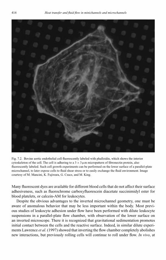
Kandlikar I044527-Ch07.tex 26/10/2005 18: 18 Page 414
414 Heat transfer and fluid flow in minichannels and microchannels
Fig. 7.2. Bovine aortic endothelial cell fluorescently labeled with phalloidin, which shows the interiorcytoskeleton of the cell. The cell is adhering to a 3 × 3 µm micropattern of fibronectin protein, alsofluorescently labeled. Such cell growth experiments can be performed on the lower surface of a parallel-platemicrochannel, to later expose cells to fluid shear stress or to easily exchange the fluid environment. Imagecourtesy of M. Mancini, K. Fujiwara, G. Csucs, and M. King.
Many fluorescent dyes are available for different blood cells that do not affect their surfaceadhesiveness, such as fluorochrome carboxyfluorescein diacetate succinimidyl ester forblood platelets, or calcein-AM for leukocytes.
Despite the obvious advantages to the inverted microchannel geometry, one must beaware of anomalous behavior that may be less important within the body. Most previ-ous studies of leukocyte adhesion under flow have been performed with dilute leukocytesuspensions in a parallel-plate flow chamber, with observation of the lower surface onan inverted microscope. There it is recognized that gravitational sedimentation promotesinitial contact between the cells and the reactive surface. Indeed, in similar dilute experi-ments Lawrence et al. (1997) showed that inverting the flow chamber completely abolishesnew interactions, but previously rolling cells will continue to roll under flow. In vivo, at

Kandlikar I044527-Ch07.tex 26/10/2005 18: 18 Page 415
Chapter 7. Biomedical applications of microchannel flows 415
Poiseuille flow
Shear flow
10
8
6
4
2
00 400
V (�m/s)
X (�
m)
200 600 800 1000
Fig. 7.3. Comparison of parabolic Poiseuille flow and linear shear flow in the vicinity of the lower wall in a200 µm microchannel. The wall shear rate has been set at 100 s−1.
physiological concentrations of red blood cells, the situation is quite different, with red cellsmigrating toward the center of the vessel and displacing the less deformable leukocytesto the near-wall region (a process called “margination”; see for instance Goldsmith andSpain, 1984). An erythrocyte-depleted plasma layer, containing leukocytes and platelets,is formed adjacent to the vessel wall. Cell collisions can promote initial contact betweenleukocytes and the vessel wall; this may help to explain how roughly equal numbers ofrolling leukocytes are visible on the upper and lower walls of intact mouse and hamstermicrovessels. There is a subtle effect of gravity in real vessels however, as evidenced by astudy by Bishop et al. (2001) who observed flow of whole blood in horizontally and ver-tically oriented microvessels in rat spinotrapezius muscle. They observed a symmetricalplasma layer in vertically oriented venules, whereas in horizontally oriented venules theplasma layer formed near the upper wall. Similarly, gravitational effects of whole bloodflow in rectangular channels can be minimized by orienting the channel vertically (Abbittand Nash, 2001), yet when optically imaging leukocytes through regions>40 µm the samecomplications of fluorescence labeling occur as described above. A theoretical comparisonof gravitational effects and normal forces at the tips of leukocyte microvilli suggest thatsurface interactions can dominate over gravity under the proper conditions (Zhao et al.,2001). To summarize, gravity plays a more important role in microchannel flow cham-ber experiments compared to in vivo. However, control experiments can be performedby density-matching the solution to the suspended cells, via addition of high-molecularweight dextran (shown to not interfere with selectin adhesion; Chen and Springer, 2001)to separate out any artifactual effects of gravitational sedimentation.
7.2.3. Lubrication approximation for a gradually converging (or diverging) channel
One potential application of microchannels in the study and manipulation of circu-lating cells is the use of very small-gap channels (H ≤ 10 µm) to continuously exert

Kandlikar I044527-Ch07.tex 26/10/2005 18: 18 Page 416
416 Heat transfer and fluid flow in minichannels and microchannels
high mechanical stresses on 8–10 µm blood cells or blood cell precursors as they passthrough such a device. Indeed, such mechanical stresses, that approximate the close-packing of cells within the bone marrow, may in fact be necessary for proper maturation ofred blood cells and explain why production of healthy red cells has proven to be so challeng-ing in vitro (Waugh et al., 2001). In such small microchannels created by the orientationof two parallel plates in close proximity to each other, whether the gap is maintained byrubber gaskets or particulate spacers, one must be concerned about the exact alignment ofthe bounding walls. Specifically, a slight tilt to either surface with respect to the primaryflow direction will create either a converging or diverging flow, which could significantlyinfluence bulk flow characteristics and design issues such as the total pressure drop acrossthe microchannel. If polystyrene slides are used as the bounding surfaces, flexing of thewall at high pressures could also result in a deviation from parallel alignment.
Figure 7.4 shows a diagram of the gradually converging channel geometry, symmetricabout the centerline x = 0. The corresponding plane Poiseuille flow solution for the velocityprofile is:
vz = H 2
8µ
(−dp
dz
)[1 −
(2x
H
)2]
(7.2)
where the differential version of the pressure drop is used, to allow generalization to aslowly varying channel cross-section. Similarly, for plane Poiseuille flow the flow rate perunit width, q is:
q = H 3
12µ
(−dp
dz
)(7.3)
For small variation in the channel spacing, (H1 − H2)/H1 1, it can be assumed that theflow will deviate from the plane Poiseuille solution only slightly. Thus, we are justified inassuming that Eqs. (7.2) and (7.3) will remain valid for the case depicted in Fig. 7.4, onlywith H as a slowly varying function of z. Since the flowrate through any cross-sectionmust be a constant, we conclude that the local pressure gradient must have the followingspatial dependence:
dp
dz∼ 1
H 3(z)(7.4)
H1 H2
X
Z
Fig. 7.4. Pressure-driven flow through a gradually converging channel. In the general case of a curved uppersurface, the position of the upper wall is defined by x = H (z).

Kandlikar I044527-Ch07.tex 26/10/2005 18: 18 Page 417
Chapter 7. Biomedical applications of microchannel flows 417
Thus, rearranging Eq. (7.3) for the local pressure drop in the gradually converging channelyields the expression:
dp
dz= − 12µq
H 3(z)(7.5)
Equation (7.5) can be integrated over the length of the channel L = z2 − z1, to give theoverall pressure drop across the converging channel,
p = −12µq∫ z2
z1
H−3(z)dz (7.6)
For a simple linear variation in channel height of the form
H (z) = H1 +(
H1 − H2
z1 − z2
)(z − z1) (7.7)
the solution to Eq. (7.6) becomes
p = −6µq
(L
H1 − H2
)[1
H 22
− 1
H 21
](7.8)
This can be compared to the pressure drop across a uniform planar channel,
p = −12µq
(L
H
)1
H 2 (7.9)
Figure 7.5 shows the ratio of the total pressure drop across the converging channel to thetotal pressure drop in a truly parallel channel evaluated at either the initial height (upper,
1.8
1.7
1.6
1.5
1.4
�p/
�p(
H1)
or
�p/
�p(
Hav
g)
�p/�p(Havg)
1.3
1.2
1.1
10 0.05 0.1 0.15 0.2 0.25
�p/�p(H1)
(H1 � H2)/H1
Fig. 7.5. Plot of the ratio of the pressure drop over a gradually converging channel to the pressure drop in aparallel channel evaluated at either the initial height (upper, solid line) or the average height (lower, dashed), asa function of the dimensionless height difference. Note from the upper curve that a dimensionless heightdifference of (H1 − H2)/H1 = 0.25 results in an increase in total pressure drop of 55% relative to a parallelchannel with a spacing of H1 (upper curve), however, evaluating the pressure drop at the mean channel height(lower curve) captures all but 5% of this increase.

Kandlikar I044527-Ch07.tex 26/10/2005 18: 18 Page 418
418 Heat transfer and fluid flow in minichannels and microchannels
solid curve) or evaluated at the average height (lower, dashed curve). Note that using theaverage height in Eq. (7.9) yields an estimate for the pressure drop in a converging channelthat is accurate to within 90%.
7.3. Microchannels and minichannels as bioreactors for long-term cell culture
Bioreactors are liquid vessels in which live populations of suspended or surface-attachedcells can be maintained for extended periods of time, either for expansion and differenti-ation of a desired cell type, or for the mass production of a biomolecule produced by thecells. Bioreactors usually feature gas and/or liquid exchange, to replenish nutrients to thecells as they are consumed and to remove waste and other products made by the cells. Whilecommercial cell-based production of small molecules (e.g., ethanol) or proteins involvesthe scale up of bioreactors to >1000 gallon tanks, there is much interest in miniaturizingbioreactors for use as bioartificial organ replacement of the pancreas (Sullivan et al., 1991),liver (Juaregui et al., 1997), and kidney (Cieslinski and Humes, 1994). These bioartificialorgans, in which one or more live cell populations are combined with artificial engineeredmaterials, must replace the following functions of the native organs (Fournier, 1999):
(i) Pancreas: The main purpose of the pancreas is to regulate glucose levels in the body byhosting insulin-producing cells in small clusters of cells called the “islets of Langer-hans”. There is a great need for the restoration of pancreatic function among thoseafflicted with insulin dependent diabetes mellitus (IDDM).
(ii) Liver: The human liver is a large (∼1500 g), highly vascularized organ that receives25% of the cardiac output, and performs a variety of crucial life functions. The liverstores and releases excess glucose, is the primary organ for fat metabolism, and pro-duces virtually all of the plasma proteins other than antibodies. The main engineeringchallenge in developing a bioartificial liver replacement is that the organ is home tonearly 250 billion hepatocyte cells, each around 25 µm in diameter!
(iii) Kidney: Among the vital responsibilities of the kidneys are filtration of, and wasteremoval from, the blood, regulation of red cell production within the bone marrow,and rapid control of blood pressure through the production of vasoactive molecules.
Microchannels and minichannels provide an excellent opportunity to maximize surfacearea available for monolayer cell attachment, while enabling good temperature regulationand rapid exchange of liquid media. Successful miniaturization of bioreactors for organreplacement could result in a device that may be comfortably worn outside the body, oreven potentially implanted within the abdominal cavity. Another potential advantage ofmicrochannels as bioreactors and the local flow environments that they are able to produceis that many cell types such as osteoblasts (bone cells) and endothelial cells (blood vessellining) have evolved to prefer constant exposure to shear stresses >1 dyne/cm and exhibitnormal phenotype only in such an environment.
7.3.1. Radial membrane minichannels for hematopoietic blood cell culture
Hematopoietic stem and precursor cells (HSPC) in the bone marrow are able to differentiateand produce all of the different types of blood cells in the body. Bone marrow cells grown

Kandlikar I044527-Ch07.tex 26/10/2005 18: 18 Page 419
Chapter 7. Biomedical applications of microchannel flows 419
Regulatedgas flow
Pumped-incell media 0 Cells plated on bottom wall
Gas phase
HGas-permeable membrane
Liquid phase Waste/recycle
X
L
Z
Fig. 7.6. Minichannel membrane bioreactor.
ex vivo maintain this pluripotent nature, and there is great interest in expanding blood cellpopulations in bioreactors for later transplantation to treat various blood disorders. Thedifficulty in growing large quantities of mammalian cells in culture is that oxygen is rapidlyconsumed and must be continuously replenished somehow. Peng and Palsson (1996) exam-ined the potential of a radial membrane bioreactor to culture primary human mononuclearcells subjected to several growth factors (interleukin-3, granulocyte-macrophage colony-stimulating factor, erythropoietin) known to induce production of white and red blood cells.Figure 7.6 shows a diagram of a radial membrane bioreactor. Cell media saturated withoxygen enters the chamber from the left-hand-side, at a well-developed laminar velocityu(x). Oxygen in the media is consumed by the cells near the lower surface. The fluid nearthe upper, gas-permeable membrane is assumed to be in equilibrium with the gas, and atthe saturation oxygen concentration CS. In such a system, the fluid velocity is chosen tobe very low – typical transit times equal about 1.33 days. For comparison, the diffusivityof oxygen in protein solutions at 37◦C has been measured to be D = 2.69 × 10⁻⁵ cm2/s(Goldstick, 1966). For a channel height of 3 mm, the characteristic time for diffusionfrom the upper membrane to the cell layer at the bottom of the channel is 1 h. Thus, inthis case convective transport can be neglected and the oxygen transport is modeled as aone-dimensional diffusion equation of the form,
D∂2C
∂x2 = 0 (7.10)
The boundary condition at the upper membrane is that the fluid is saturated with oxygen:
C = CS @ x = H (7.11)
and at the lower wall the flux is equal to the cellular uptake rate N0:
N0 = D∂C
∂x@ x = 0 (7.12)
Kandlikar I044527-Ch07.tex 26/10/2005 18: 18 Page 420
420 Heat transfer and fluid flow in minichannels and microchannels
Subject to these two conditions the solution to Eq. (7.10) is simply a linear concentrationprofile,
C(x) = CS + N0
D(x − H ) (7.13)
The uptake rate N0 obeys Michaelis–Menten kinetics given by:
N0 = qXC0
Km + C0(7.14)
where C0 is the oxygen concentration at the lower wall, that is, the oxygen concentrationexperienced by the cells, q is the oxygen uptake rate on a per-cell basis, and X is thecell density. The Michaelis constant Km, which can be interpreted as the concentrationat which the uptake rate is half-maximum, has been measured to be about 1–5% of CS(Ozturk, 1990). This implies that the oxygen consumption operates at near zeroeth-orderkinetics. Substituting Eq. (7.14) into Eq. (7.13) and evaluating the solution at x = 0 yieldsa quadratic expression for C0:
C20 + (Km − CS + qXH /D)C0 − CSKm = 0 (7.15)
In terms of the fractional saturation σ= C/CS, Eq. (7.15) becomes,
σ20 + (κ + φ − 1)σ0 − κ = 0 (7.16)
where we have introduced two dimensionless parameters, a dimensionless Michaelisconstant κ= Km/CS, and
φ = qXH /DCS = H 2/D
HCS/qX(7.17)
which is the ratio of the characteristic time for diffusion to the characteristic time forcellular oxygen uptake. The parameter φ depends on the cell density, which changes withtime as the cells on the surface divide and double in number every 24–48 h. There is onlyone physically reasonable root to Eq. (7.16), since the other will always be negative. Thisfractional saturation design equation can be used to determine the range of parametervalues for which the cells receive sufficient oxygen to support proliferation.
7.3.2. The Bioartificial liver: membranes enhance mass transfer inplanar microchannels
Many types of cells can be grown in vitro more successfully when co-cultured in thepresence of a second cell type such as 3T3-J2 fibroblasts, which are robust and can producevital nutrients that support the growth of the cells of interest. Tilles et al. (2001) studiedthe co-culture of rat hepatocytes (liver cells) with 3T3-J2 fibroblasts in microchannel

Kandlikar I044527-Ch07.tex 26/10/2005 18: 18 Page 421
Chapter 7. Biomedical applications of microchannel flows 421
Cell layer
Solid wall
Z
X
(a) (b)
UC0 UC0
Cg
Polyurethanemembrane
H
Fig. 7.7. Microchannel bioreactors (a) without and (b) with an internal membrane oxygenator.
bioreactors (H = 85–500 µm). Their analysis of the effects that an oxygenating membranehas on hepatocyte growth and protein production (see Fig. 7.7) provides a useful set ofdesign equations for the development of microchannel membrane-based bioreactors.
For simplicity, we assume uniform, or “plug”, flow within the microchannel (see Prob-lem 7.4 for a modification of this approximation). The flow direction is defined withthe z-coordinate, and oxygen diffusion occurs in the x-direction normal to the walland is consumed by hepatocytes at x = 0. Once the oxygen concentration C(x, z) isnon-dimensionalized with the inlet concentration Cin, and the x and z variables non-dimensionalized with the height (H ) and length (L) of the bioreactor, respectively, thenthe dimensionless steady-state convection-diffusion equation becomes
∂C∗
∂z= γ
Pe
∂2C∗
∂x2 (7.18)
Where we have introduced the dimensionless length ratio γ = L/H , and the Peclet numberPe = UH /D. Here U is the average velocity and D is the oxygen diffusivity. The boundaryconditions for Eq. (7.18) are
C∗ = 1 @ z = 0, 0 ≤ x ≤ 1
∂C∗
∂x= Da @ x = 0, 0 ≤ z ≤ 1
∂C∗
∂x={
0Sh[C∗
g − C∗]@ x = 1,@ x = 1,
0 ≤ z ≤ 10 ≤ z ≤ 1
(7.19)
where there exist two different flux conditions at the upper surface depending on whetherthere is no membrane oxygenation, or with membrane oxygenation. We have introducedtwo additional dimensionless groups, the Damkohler number
Da = VmHX
DCin(7.20)
and the Sherwood number
Sh = σH
D(7.21)

Kandlikar I044527-Ch07.tex 26/10/2005 18: 18 Page 422
422 Heat transfer and fluid flow in minichannels and microchannels
where the zeroeth-order uptake of oxygen by the hepatocytes is defined as Vm, the surfacedensity of cells as X , and σ is the membrane permeability to oxygen. We have non-dimensionalized the gas phase oxygen concentration with Cin as C∗
g = Cg/Cin. A similardifferential system has been solved analytically be Carslaw and Jaeger (1959), which canbe applied to yield the cell surface oxygen concentration along the length of the bioreactoreither without internal membrane oxygenation:
C∗(0, z) = 1 − zγ
PeDa − Da
3+ 2Da
π2
∞∑n=1
(−1)n
n2 cos(nπ) exp[−γn2π2z
Pe
](7.22)
or with internal membrane oxygenation:
C∗(0, z) = C∗g − Da − Da
Sh+
∞∑n=1
Bn exp[−γλ2
nz
Pe
](7.23)
In Eq. (7.23), the coefficients Bn are defined by:
Bn = 4Da(1 − cos λn) + 4λn sin λn(1 − C∗g + Da/Sh)
[λn sin 2λn + 2λ2n]
(7.24)
and λn are the roots of the transcendental equation:
tan λn = Sh
λn(7.25)
Example 7.1 (see page 434) illustrates the use of these design equations (7.22–7.25).
7.3.3. Oxygen and lactate transport in micro-grooved minichannels for cell culture
As stated in Section 7.3.1, there is considerable interest in culturing and expandinghematopoietic stem cell populations ex vivo, for later autologous (donor = recipient)or allogeneic (donor �= recipient) transplantation for the treatment of hematological orimmunological disorders and to treat complications of cancer therapies. In their nativeenvironment in the bone marrow, hematopoietic cells are not strongly adherent to theirsurroundings but are retained in the marrow in part due to adhesion to a second type ofcells called stromal cells. It has been recognized that ex vivo cell perfusion systems forlong-term culture that are able to retain weakly adherent cells would hold many advantagesover co-culture systems (Sandstrom et al., 1996). Horner et al. (1998) analyzed the solutetransport in a micro-grooved minichannel designed to retain non-adherent cells withinmicroscale cavities oriented perpendicular to the main flow, as depicted in Fig. 7.8. Flowthrough the main minichannel generates a form of lid-driven flow within each cavity knownas nested Moffatt eddies (Moffatt, 1964). These eddies provide convection-enhanced masstransfer between the cells resting at the bottom of each cavity and the main chamber,while sheltering the cells from the high wall shear stresses that would be experienced in acomparable flat-bottomed channel.

Kandlikar I044527-Ch07.tex 26/10/2005 18: 18 Page 423
Chapter 7. Biomedical applications of microchannel flows 423
5 mm channel
X
Z
200 �m
Fig. 7.8. Micro-grooved, minichannel bioreactor for the culture of weakly adherent cells. Note that the cells aresheltered within the grooves and do not become entrained in the flow. The exterior flow induces Moffett eddiesthat exchange solutes between the groove cavities and the minichannel region.
For a relatively wide channel of several centimeters, the aspect ratio is such that thethird dimension (vorticity direction) can be neglected and the problem treated as two-dimensional. As in our previous bioreactor examples, we take the flow direction as zand the velocity gradient direction as x. At steady-state, the Navier–Stokes equation intwo-dimensions simplifies to:
ρ
(vx∂vx
∂x+ vz
∂vx
∂z
)= −∂p
∂x+ µ
(∂2vx
∂x2 + ∂2vx
∂z2
)
ρ
(vx∂vz
∂x+ vz
∂vz
∂z
)= −∂p
∂z+ µ
(∂2vz
∂x2 + ∂2vz
∂z2
) (7.26)
Note that unlike previous examples where the flow was assumed unidirectional in thez-direction and diffusion in the z-direction neglected relative to convection, leading tosimplifications to the governing equations, the lid-driven cavity flow is expected to befully two-dimensional and these full equations must be integrated. The solute balance forspecies i, at steady-state, takes the form:
vx∂Ci
∂x+ vz
∂Ci
∂z= −Di
(∂2Ci
∂x2 + ∂2Ci
∂z2
)(7.27)
The solutes of main biological interest (oxygen and lactate) are dilute small molecules thatdo not appreciably affect the fluid density and viscosity. Thus, the fluid velocity field may
Kandlikar I044527-Ch07.tex 26/10/2005 18: 18 Page 424
424 Heat transfer and fluid flow in minichannels and microchannels
be solved independently of the solute balance equation. It is reasonable to impose a well-developed parabolic velocity profile at the channel inlet, provided that the cell-containingregion occurs after the entrance length given by:
Lent
H= aRe (7.28)
where the Reynolds number is defined for channel flow as:
Re = ρ〈v〉Hµ
(7.29)
In Eq. (7.28), the coefficient a is equal to 0.034 to ensure that the centerline velocity iswithin 98% of the theoretical Poiseuille flow limit (Bodoia and Osterle, 1961), and theangled brackets denote an averaged quantity. For typical bioreactor conditions, the entrancelength is reached within a fraction of one channel height (<0.05H ). No-slip conditions areenforced at the upper, lower, and micro-groove walls. The general flux condition at the lowerwall of the micro-groove cavities, plated with hematopoietic cells, is obtained by settingthe surface solute flux equal to a Michaelis–Menten kinetic rate of solute consumptionor production (e.g., oxygen or lactate, respectively). This boundary condition at the cellsurface takes the form:
N0 = −D∂C
∂x= qXC0
Km + C0(7.30)
where a sign change from Eq. (7.12) is introduced for a local coordinate system withinthe cavity corresponding to an upper cavity opening at x = 0 and the positive x-coordinatedirected downward. The system of Eqs. (7.26), (7.27), and (7.30), subject to no-slip at thewall and given inlet velocity and solute concentration conditions, can be readily solvedfor the spatial concentration profiles using a commercial computational fluid dynamics(CFD) code such as FIDAP (Fluent, Inc., Lebanon, NH). Horner et al. (1998) have usedfull numerical analysis of the micro-grooved minichannel system to derive constitutiveequations that describe the solute concentration within the groove cavities as a functionof various physical parameters such as flowrate, channel dimensions, and zeroeth-ordersolute consumption (production) rate.
7.4. Generation of normal forces in cell detachment assays
Hydrodynamic flow in parallel-plate microchannels is often used to detach firmly adheredcells from substrates, as a measure of the strength of integrin:matrix protein bonds(Fig. 7.9). However, the high flowrates necessary to detach spread cells, when flowingover a flat cell with a raised nuclear region, may produce a negative pressure over thenucleus (the so-called “Bernoulli effect”) that can potentially equal or exceed the shearforces that one is trying to generate (Fig. 7.10). Thus, here we model this problem asinviscid, irrotational flow over a wavy wall as developed by Michelson (1970), keeping
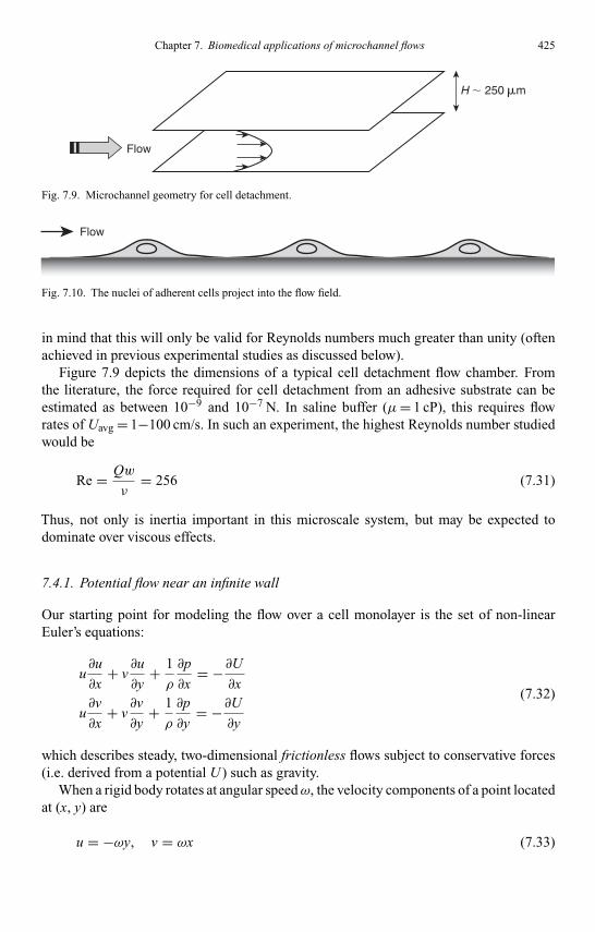
Kandlikar I044527-Ch07.tex 26/10/2005 18: 18 Page 425
Chapter 7. Biomedical applications of microchannel flows 425
Flow
H � 250 �m
Fig. 7.9. Microchannel geometry for cell detachment.
Flow
Fig. 7.10. The nuclei of adherent cells project into the flow field.
in mind that this will only be valid for Reynolds numbers much greater than unity (oftenachieved in previous experimental studies as discussed below).
Figure 7.9 depicts the dimensions of a typical cell detachment flow chamber. Fromthe literature, the force required for cell detachment from an adhesive substrate can beestimated as between 10−9 and 10−7 N. In saline buffer (µ= 1 cP), this requires flowrates of Uavg = 1−100 cm/s. In such an experiment, the highest Reynolds number studiedwould be
Re = Qw
ν= 256 (7.31)
Thus, not only is inertia important in this microscale system, but may be expected todominate over viscous effects.
7.4.1. Potential flow near an infinite wall
Our starting point for modeling the flow over a cell monolayer is the set of non-linearEuler’s equations:
u∂u
∂x+ v
∂u
∂y+ 1
ρ
∂p
∂x= −∂U
∂x
u∂v
∂x+ v
∂v
∂y+ 1
ρ
∂p
∂y= −∂U
∂y
(7.32)
which describes steady, two-dimensional frictionless flows subject to conservative forces(i.e. derived from a potential U ) such as gravity.
When a rigid body rotates at angular speedω, the velocity components of a point locatedat (x, y) are
u = −ωy, v = ωx (7.33)
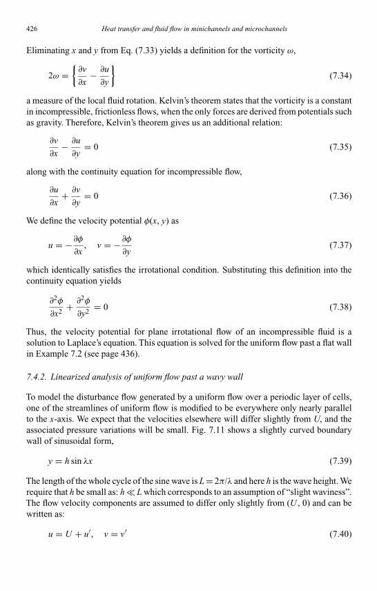
Kandlikar I044527-Ch07.tex 26/10/2005 18: 18 Page 426
426 Heat transfer and fluid flow in minichannels and microchannels
Eliminating x and y from Eq. (7.33) yields a definition for the vorticity ω,
2ω ={∂v
∂x− ∂u
∂y
}(7.34)
a measure of the local fluid rotation. Kelvin’s theorem states that the vorticity is a constantin incompressible, frictionless flows, when the only forces are derived from potentials suchas gravity. Therefore, Kelvin’s theorem gives us an additional relation:
∂v
∂x− ∂u
∂y= 0 (7.35)
along with the continuity equation for incompressible flow,
∂u
∂x+ ∂v
∂y= 0 (7.36)
We define the velocity potential φ(x, y) as
u = −∂φ
∂x, v = −∂φ
∂y(7.37)
which identically satisfies the irrotational condition. Substituting this definition into thecontinuity equation yields
∂2φ
∂x2 + ∂2φ
∂y2 = 0 (7.38)
Thus, the velocity potential for plane irrotational flow of an incompressible fluid is asolution to Laplace’s equation. This equation is solved for the uniform flow past a flat wallin Example 7.2 (see page 436).
7.4.2. Linearized analysis of uniform flow past a wavy wall
To model the disturbance flow generated by a uniform flow over a periodic layer of cells,one of the streamlines of uniform flow is modified to be everywhere only nearly parallelto the x-axis. We expect that the velocities elsewhere will differ slightly from U, and theassociated pressure variations will be small. Fig. 7.11 shows a slightly curved boundarywall of sinusoidal form,
y = h sin λx (7.39)
The length of the whole cycle of the sine wave is L = 2π/λ and here h is the wave height. Werequire that h be small as: h L which corresponds to an assumption of “slight waviness”.The flow velocity components are assumed to differ only slightly from (U , 0) and can bewritten as:
u = U + u′, v = v′ (7.40)
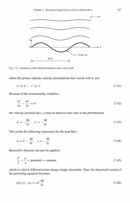
Kandlikar I044527-Ch07.tex 26/10/2005 18: 18 Page 427
Chapter 7. Biomedical applications of microchannel flows 427
0
y
x
U
2p/ly � h sin lx
Fig. 7.11. Geometry of the linearized analysis near a wavy wall.
where the primes indicate velocity perturbations that vanish with h, and
u′ U , v′ U (7.41)
Because of the irrotationality condition,
∂v′
∂x− ∂u′
∂y= 0 (7.42)
the velocity potential φ(x, y) may be taken to refer only to the perturbations
u′ = −∂φ
∂x, v′ = −∂φ
∂y(7.43)
This yields the following expression for the total flow:
u = U − ∂φ
∂x, v = −∂φ
∂y(7.44)
Bernoulli’s theorem can now be applied:
u2
2+ p
ρ+ potential = constant (7.45)
which is valid at different points along a single streamline. Thus, the linearized version ofthe governing equation becomes
p(x, y) − p0 = ρU∂φ
∂x(7.46)

Kandlikar I044527-Ch07.tex 26/10/2005 18: 18 Page 428
428 Heat transfer and fluid flow in minichannels and microchannels
where we have subtracted off the quantity p0 + ρU 2 = cst. evaluated far from the wall. InEq. (7.46), p0 denotes the pressure in those parts of the flow where the velocity reaches itsuniform value U.
The velocity potential is a harmonic function given by the equation
∂2φ
∂x2 + ∂2φ
∂y2 = 0 (7.47)
We must now find the particular solution to Eq. (7.47) out of the many general solutionsto Laplace’s equation. First, we note the farfield condition φ(x, ∞) = 0. At the boundary,we enforce that the slope of the velocity vector equals the boundary slope:
v
u= hλ cos λx (7.48)
From our earlier development, the left-hand-side of Eq. (7.48) is given by
LHS = − ∂φ/∂y
U − ∂φ/∂x= − 1
U
∂φ
∂y(7.49)
where we have neglected higher order terms. We may write an approximate boundarycondition evaluated at y = 0:
−∂φ
∂y(x, 0) = Uhλ cos λx (7.50)
Note that the differential equation, boundary conditions, and pressure relationship are alllinear in φ-derivatives. This problem admits a separable solution of the form:
X (x) = A cos k x + B sin k xY (y) = C exp(−k y) + D exp(k y)
(7.51)
which combine to give the following potential function:
φ(x, y) = {A cos k x + B sin k x}{C exp(−k y)+D exp(ky)} (7.52)
where the term D exp(ky) vanishes in order to satisfy the farfield condition. We are thusleft with two remaining constants AC and BC, and can set C = 1 without loss of generality.The boundary condition at y = 0 takes the form
Uhλ cos λx = k{A cos k x + B sin k x} (7.53)
which, upon manipulation, yields the result
Uhλ = kA, B = 0, k = λ (7.54)
These constants can be inserted into our general solution to give
φ(x, y) = Uh exp(−λy) cos λx (7.55)

Kandlikar I044527-Ch07.tex 26/10/2005 18: 18 Page 429
Chapter 7. Biomedical applications of microchannel flows 429
p �����
p ����
Fig. 7.12. Pressure distribution at the surface of the wall.
for the velocity potential, and the following expression for the pressure at any point inthe flow:
p(x, y) = p0 − ρU 2hλ sin λx exp(−λy) (7.56)
Thus, the linear approximation to the pressure on the boundary wall y = 0 is
p(x, 0) = p0 − ρU 2hλ sin λx (7.57)
Equation (7.57) implies that the pressure is a minimum at the peaks of the wavy wall(λx =π/2) and reaches a maximum at the wave troughs, as depicted in Fig. 7.12.
Typical parameter values for cell detachment experiments yield the following estimatefor the peak (negative) pressure above the cell nucleus:
ρU 2hλ = (1000 kg/m3)(1 m/s)2(2 × 10−6 m)(2π/20 × 10−6 m) (7.58)
Thus, the pressure above the cell nucleus is predicted to have magnitude p = 628 N/m2,or assuming a characteristic cell area of 100 µm2, a negative pressure of magnitudeF = |63 nN|. This value for the normal force induced by the Bernoulli effect is of thesame order as the shear forces generated by the imposed flow! Reanalysis of many previ-ous experiments using cell detachment assays show the generation of large normal forcesin both the microchannel geometry (VanKooten et al., 1992; Schnittler et al., 1993; Sanket al., 1994; Thompson et al., 1994; Wechazak et al., 1994; Kapur and Randolph, 1998;Sirois et al., 1998; Chan et al., 1999; Malek et al., 1999; Grandas et al., 2001) as well asthe spinning disk assay (Garcia et al., 1997; Boettiger et al., 2001; Deligianni et al., 2001;Miller and Boettiger, 2003). To reduce the Reynolds number, and thus reduce the normalforces relative to shear forces, one should simply increase the fluid viscosity with a high-molecular weight molecule such as dextran. For instance, a 7.5 weight percent dextransolution, of molecular weight MW = 2 × 10⁶ g/mol, would result in a relative viscosity of
µ
µ0= 20.5
7.5. Small-bore microcapillaries to measure cell mechanics and adhesion
The human circulatory system represents a challenging system for engineering model-ing, due to the wide variation in vessel geometry, linear flow velocity, and Reynolds

Kandlikar I044527-Ch07.tex 26/10/2005 18: 18 Page 430
430 Heat transfer and fluid flow in minichannels and microchannels
Table 7.2Typical flow parameters in the human systemic circulation.
Structure Diameter (cm) Blood velocity (cm/s) Tube Reynolds number
Ascending aorta 2.0–3.2 63 3600–5800Descending aorta 1.6–2.0 27 1200–1500Large arteries 0.2–0.6 20–50 110–850Arterioles 0.001–0.015 0.5–1.0 0.014–0.43Capillaries 0.0005–0.001 0.05–0.1 0.0007–0.003Venules 0.001–0.02 0.1–0.2 0.0029–0.11Large veins 0.5–1.0 15–20 210–570Vena cavae 2.0 11–16 630–900
Data from Cooney, 1976; Whitmore, 1968; Schneck, 2000.
numbers, starting at the major aortic vessels down to the smallest microscopic capillar-ies. Table 7.2 shows the range of these values in a typical human, assuming a constantblood viscosity of 0.035 P and mean peak velocities reported for the pulsatile flow ofarterial flow.
It is evident that the human circulation covers the entire range of flow behavior fromcreeping (non-inertial) flow up to fully developed turbulence. We see in the arterioles,capillaries, and venules that the length scales span the range of fluid physics encounteredin microchannel and minichannel flow. In the largest vessels of the body, blood behavesas a non-Newtonian fluid and constitutive equations are usually successful in describingbehavior (e.g. blunted velocity profiles) at the continuum level. At the scale of the smallestvessels however, the particulate nature of blood and its constituent cells must be taken intoaccount (King et al., 2004). In the capillaries of the lungs, for instance, the mechanicalproperties of individual white blood cells significantly influence the transit time throughthese vessels (Bathe et al., 2002).
Suspensions of erythrocytes (red blood cells, or RBCs) flowing through microcapillaries(d ∼ 40 µm) are well known to concentrate at the tube center, resulting in velocity profilesblunted from parabolic. Trajectories of individual RBCs have been visualized both in vitro(Goldsmith and Marlow, 1979) and in vivo (Lominadze and Mchedlishvili, 1999), showingradial drift velocities and random walks that attenuate as the cell approaches the center-line. The single-file motion of RBCs through small capillaries (d ∼ 4–20 µm) has beenmodeled theoretically subject to various simplifying assumptions: x–y two-dimensionality(Sugihara-Seki et al., 1990), symmetry about the center axis (Secomb and Hsu, 1996), orapproximation via multipole expansion (Olla, 1999). The radial drift of RBCs is knownto produce a cell-free plasma layer in microvessels (Yamaguchi et al., 1992), suggestingthat RBCs have only a secondary influence on the dynamics of leukocytes once they aredisplaced to the vessel wall (Goldsmith and Spain, 1984). Furthermore, leukocytes have adramatic influence on total blood viscosity in the microcirculation despite their relativelylow numbers in blood as compared to RBCs (Helmke et al., 1998), highlighting the needto better understand the motion of leukocytes through microcapillaries.
Example 7.3 (see page 437) provides an estimate of the blood transit time through acapillary, where the majority of oxygen exchange takes place.

Kandlikar I044527-Ch07.tex 26/10/2005 18: 18 Page 431
Chapter 7. Biomedical applications of microchannel flows 431
Cellsample
Sheathfluid
Hydrodynamicfocusingregion
Forwardscatter
detector
Side scatterdetector
Laser
Charged plates tosteer cells to the
left or right
� �
Fig. 7.13. Schematic of a flow cytometer, and fluorescence activated cell sorting (FACS).
7.5.1. Flow cytometry
Flow cytometry is a powerful analysis tool in biomedical research, that utilizes microscaleflow for automated single cell characterization and sorting. The concentration of anyfluorescently labeled molecule on the surface of the cell can be measured relative to somestandard, and these cells can furthermore be sorted according to the concentration of thismarker or according to size. Antibodies against many of the known receptors on the surfaceof human or animal cells can be obtained commercially. Figure 7.13 shows a schematicof a typical system. The cell suspension (possibly containing a mixture of different celltypes) is introduced through a circular conduit. This conduit opens into a larger flowdomain containing a flowing annulus of “sheath fluid” which acts to focus the streamof cells into a single-file configuration within a narrow jet of fluid (<100 µm diameter).This stream of cells then passes through a quartz chamber where they are characterizedfor their scattering and fluorescent properties. Most commonly, a beam of light froman argon laser is used to excite the fluorophore of interest. The emitted light from this

Kandlikar I044527-Ch07.tex 26/10/2005 18: 18 Page 432
432 Heat transfer and fluid flow in minichannels and microchannels
fluorophore is then collected at one of two photomultiplier tubes. Downstream of theseoptics, the outlet stream is ruptured into a series of droplets, each containing a single cell,via piezoelectric vibration. An electrical field is then used to steer positively or negativelycharged individual droplets (a charge imposed depending on the previous fluorescenceintensity of the corresponding cell) into multiple collection vessels. The whole process isautomated so that commercially available flow cytometers can sort cells at a rate of over104 cells/s. In addition to characterizing individual cells for clinical applications, flowcytometry has been used to measure the size of small blood cell aggregates, where up topentuplets of neutrophils can be successfully identified (Simon et al., 1990; Neelameghamet al., 2000).
7.5.2. Micropipette aspiration
Small-bore glass microcapillaries are often used to either characterize the mechanics anddeformability of individual cells, or to test the surface adhesion of cells contacting othercells or artificial bead surfaces (Lomakina et al., 2004; Spillmann et al., 2004). Capillarieswith inner diameter less than the major diameter of cells such as blood cells are used topartially aspirate the cell, with the projection length of the cell within the capillary interiorbeing a measure of the cortical tension of the cell exterior (Herant et al., 2003). Once thecell is ejected from the micropipette, its shape recovery can also yield information on theviscoelastic parameters of the cell (Dong et al., 1988). Capillaries with inner diameterlarger than the cell diameter can be used to translate the cell back and forth within thepipette to bring a cell into repeated contact with another nearby surface. In this manner,the probability for cell adhesion can be determined in the presence of various biologicalstimuli. Shao and Hochmuth (1996) calculated the pressure drop caused by the gap flowin the annular region between a spherical cell and a larger cylindrical micropipette. Thegeometry considered is depicted in Fig. 7.14.
Assuming axisymmetric flow, and neglecting inertia, yields the following form of theNavier–Stokes equations in cylindrical coordinates:
1
r
∂
∂r(ru) + ∂w
∂z= 0
∂p
∂r= µ
(∂2u
∂r2 + 1
r
∂u
∂r− u
r2 + ∂2u
∂z2
)
∂p
∂z= µ
(∂2w
∂r2 + 1
r
∂w
∂r+ ∂2w
∂z2
)(7.59)
where p is the pressure, u and w are the local fluid velocities in the r- and z-directions,respectively, and µ is the fluid viscosity. No-slip conditions are enforced at all bound-aries, and the total volumetric flowrate through any circular cross-section of the pipetteis a constant Q. After considerable manipulations, useful analytical expressions can beobtained relating the total pressure drop p, sphere velocity U , and external force actingon the sphere F , for two simplified cases: (i) stationary sphere, and (ii) force-free sphere.
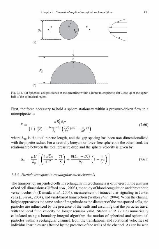
Kandlikar I044527-Ch07.tex 26/10/2005 18: 18 Page 433
Chapter 7. Biomedical applications of microchannel flows 433
U FDs
(a)
(b)
Rp
ε
r
z
Fig. 7.14. (a) Spherical cell positioned at the centerline within a larger micropipette. (b) Close-up of the upperhalf of the cylindrical region.
First, the force necessary to hold a sphere stationary within a pressure-driven flow in amicropipette is:
F = πR2pp(
1 + 43 ε)+ 8(Leq−Ds)
Rp
(2√
29π ε5/2 − 8
9π2 ε3) (7.60)
where Leq is the total pipette length, and the gap spacing has been non-dimensionalizedwith the pipette radius. For a neutrally buoyant or force-free sphere, on the other hand, therelationship between the total pressure drop and the sphere velocity is given by:
p = µU
Rp
[(4√
2π
ε1/2− 71
5
)+ 8
(Leq − Ds
)Rp
(1 − 4
3ε
)](7.61)
7.5.3. Particle transport in rectangular microchannels
The transport of suspended cells in rectangular microchannels is of interest in the analysisof red cell dimensions (Gifford et al., 2003), the study of blood coagulation and thromboticvessel occlusion (Kamada et al., 2004), measurement of intracellular signaling in Jurkatcells (Li et al., 2004), and viral-based transfection (Walker et al., 2004). When the channelheight approaches the same order of magnitude as the diameter of the transported cells, theparticles are influenced by the presence of the walls and assuming that the particles travelwith the local fluid velocity no longer remains valid. Staben et al. (2003) numericallycalculated using a boundary-integral algorithm the motion of spherical and spheroidalparticles within a rectangular channel. Both the translational and rotational velocities ofindividual particles are affected by the presence of the walls of the channel. As can be seen
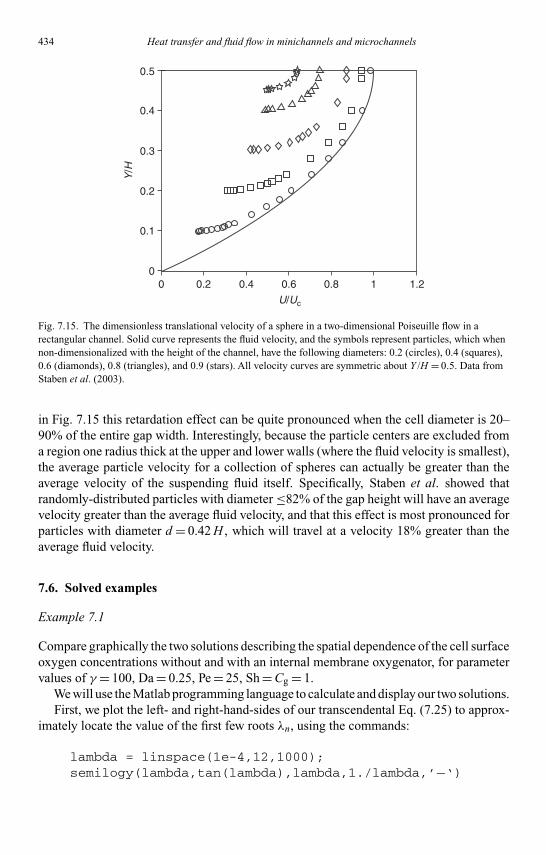
Kandlikar I044527-Ch07.tex 26/10/2005 18: 18 Page 434
434 Heat transfer and fluid flow in minichannels and microchannels
0
0.1
0.2 0.4 0.6 0.8 1 1.20
0.2
Y/H
U/Uc
0.3
0.4
0.5
Fig. 7.15. The dimensionless translational velocity of a sphere in a two-dimensional Poiseuille flow in arectangular channel. Solid curve represents the fluid velocity, and the symbols represent particles, which whennon-dimensionalized with the height of the channel, have the following diameters: 0.2 (circles), 0.4 (squares),0.6 (diamonds), 0.8 (triangles), and 0.9 (stars). All velocity curves are symmetric about Y /H = 0.5. Data fromStaben et al. (2003).
in Fig. 7.15 this retardation effect can be quite pronounced when the cell diameter is 20–90% of the entire gap width. Interestingly, because the particle centers are excluded froma region one radius thick at the upper and lower walls (where the fluid velocity is smallest),the average particle velocity for a collection of spheres can actually be greater than theaverage velocity of the suspending fluid itself. Specifically, Staben et al. showed thatrandomly-distributed particles with diameter ≤82% of the gap height will have an averagevelocity greater than the average fluid velocity, and that this effect is most pronounced forparticles with diameter d = 0.42 H , which will travel at a velocity 18% greater than theaverage fluid velocity.
7.6. Solved examples
Example 7.1
Compare graphically the two solutions describing the spatial dependence of the cell surfaceoxygen concentrations without and with an internal membrane oxygenator, for parametervalues of γ = 100, Da = 0.25, Pe = 25, Sh = Cg = 1.
We will use the Matlab programming language to calculate and display our two solutions.First, we plot the left- and right-hand-sides of our transcendental Eq. (7.25) to approx-
imately locate the value of the first few roots λn, using the commands:
lambda = linspace(1e-4,12,1000);semilogy(lambda,tan(lambda),lambda,1./lambda,’−‘)
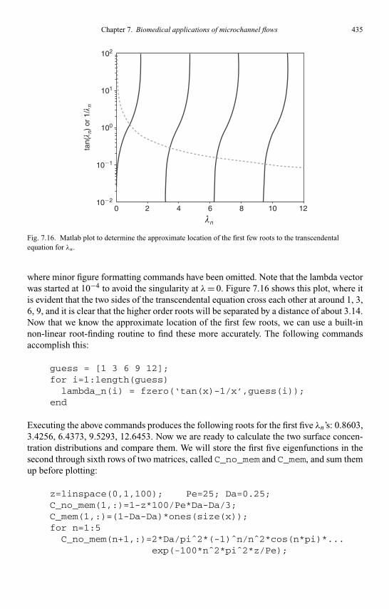
Kandlikar I044527-Ch07.tex 26/10/2005 18: 18 Page 435
Chapter 7. Biomedical applications of microchannel flows 435
102
101
100
0 2 4
λn
tan(
λ n)
or 1
/λn
6 8 10 12
10�1
10�2
Fig. 7.16. Matlab plot to determine the approximate location of the first few roots to the transcendentalequation for λn.
where minor figure formatting commands have been omitted. Note that the lambda vectorwas started at 10−4 to avoid the singularity at λ= 0. Figure 7.16 shows this plot, where itis evident that the two sides of the transcendental equation cross each other at around 1, 3,6, 9, and it is clear that the higher order roots will be separated by a distance of about 3.14.Now that we know the approximate location of the first few roots, we can use a built-innon-linear root-finding routine to find these more accurately. The following commandsaccomplish this:
guess = [1 3 6 9 12];for i=1:length(guess)
lambda_n(i) = fzero(‘tan(x)-1/x’,guess(i));end
Executing the above commands produces the following roots for the first five λn’s: 0.8603,3.4256, 6.4373, 9.5293, 12.6453. Now we are ready to calculate the two surface concen-tration distributions and compare them. We will store the first five eigenfunctions in thesecond through sixth rows of two matrices, called C_no_mem and C_mem, and sum themup before plotting:
z=linspace(0,1,100); Pe=25; Da=0.25;C_no_mem(1,:)=1-z*100/Pe*Da-Da/3;C_mem(1,:)=(1-Da-Da)*ones(size(x));for n=1:5
C_no_mem(n+1,:)=2*Da/piˆ2*(-1)ˆn/nˆ2*cos(n*pi)*...exp(-100*nˆ2*piˆ2*z/Pe);
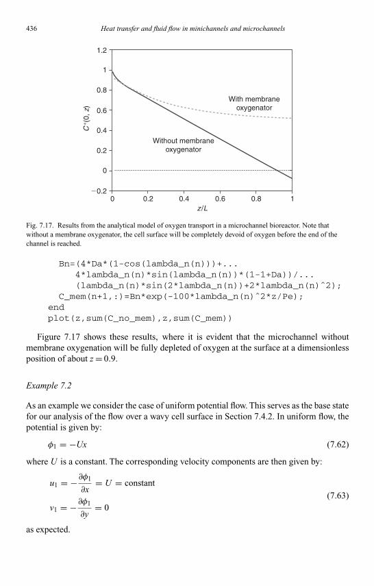
Kandlikar I044527-Ch07.tex 26/10/2005 18: 18 Page 436
436 Heat transfer and fluid flow in minichannels and microchannels
1.2
0.8
0.6
With membraneoxygenator
Without membraneoxygenator
0.4
0.2
�0.2
C∗ (
0, z
)
0 0.2 0.4z /L
0.6 0.8 1
0
1
Fig. 7.17. Results from the analytical model of oxygen transport in a microchannel bioreactor. Note thatwithout a membrane oxygenator, the cell surface will be completely devoid of oxygen before the end of thechannel is reached.
Bn=(4*Da*(1-cos(lambda_n(n)))+...4*lambda_n(n)*sin(lambda_n(n))*(1-1+Da))/...(lambda_n(n)*sin(2*lambda_n(n))+2*lambda_n(n)ˆ2);
C_mem(n+1,:)=Bn*exp(-100*lambda_n(n)ˆ2*z/Pe);endplot(z,sum(C_no_mem),z,sum(C_mem))
Figure 7.17 shows these results, where it is evident that the microchannel withoutmembrane oxygenation will be fully depleted of oxygen at the surface at a dimensionlessposition of about z = 0.9.
Example 7.2
As an example we consider the case of uniform potential flow. This serves as the base statefor our analysis of the flow over a wavy cell surface in Section 7.4.2. In uniform flow, thepotential is given by:
φ1 = −Ux (7.62)
where U is a constant. The corresponding velocity components are then given by:
u1 = −∂φ1
∂x= U = constant
v1 = −∂φ1
∂y= 0
(7.63)
as expected.

Kandlikar I044527-Ch07.tex 26/10/2005 18: 18 Page 437
Chapter 7. Biomedical applications of microchannel flows 437
Example 7.3
Consider the demand for effective mass transport in the microcirculation. Cooney (1976)showed through simple scaling arguments that the rate of mass transport rates across bloodcapillaries must be quite effective owing to the relatively short residence time of bloodin these vessels. The typical capillary diameter is about 8 µm, which allows deformablered and white blood cells (d ∼ 8–10 µm) to squeeze through these smallest vessels. Thenumber of systemic capillaries in the body can be estimated to be about n = 109, and thecardiac output about Q = 5 l/min. Thus, the linear velocity of blood flow in the capillariescan be readily calculated as:
v = Q
nπr2 = 5000 cm3/min
109(3.142)(4 × 10⁻⁴ cm)2 = 9.95 cm/min = 0.166 cm/s (7.64)
If we assume that each capillary is 1 mm long, the characteristic blood residence time inthe capillary is thus:
t = 1 mm
1.66 mm/s= 0.6 s (7.65)
Thus, mass transfer of metabolites and waste products through the capillary wall cannotencounter much barrier to mass transport since so little time for exchange is providedbefore the blood begins flowing back through the arterial tree back to the heart.
7.7. Practice problems
1. Calculate the velocity profile for a radial flow assay as a function of r and z, in termsof the volumetric flowrate and the channel dimensions. Neglect the central region andassume that the inlet radius is small. Then, use your solution for the velocity field toderive the wall shear stress expression given by Eq. (7.1).
2. Consider a slowly converging channel. Assuming a desired gap height of H = 8 µm,a channel width and length of W = 25 mm and L = 75 mm, respectively, but an actualgap height achieved of H1 = 8 and H2 = 7 µm, calculate the required pressure headby neglecting the additional pressure drop across fittings and tubing. Based on yourvalue, will gravity-driven flow or a commercially available syringe pump be moreappropriate for this application? Noting that the wall shear stress varies as the inverseof H squared, will the average wall shear stress within the channel simply be that fora straight channel using the average channel height? Calculate the average wall shearstress in such a channel, for arbitrary height change, by computing the area-averagedintegral of the wall shear stress down the length of the flow domain.
3. Calculate the total pressure drop in a microchannel that experiences a symmetric buck-ling of the upper and lower walls in a parabolic shape, in terms of the fluid properties,flow rate, the initial/final height, and the height at the center of the channel. How much

Kandlikar I044527-Ch07.tex 26/10/2005 18: 18 Page 438
438 Heat transfer and fluid flow in minichannels and microchannels
Table 7.3Parameter values for hepatocyte/3T3 fibroblastco-culture in a microchannel bioreactor.
Parameter Value
H 100 µmα 105 hepatocytes/cm2
Q 0.1 mL/minU 7 × 10⁻² cm/sVm 0.4 nmol/s per 106 cellsσ 5 µm/sD 2 × 10⁻⁵ cm2/sPe 30Da 0.1Sh 0.25
error is introduced by only measuring the gap height in the center of the channel andassuming that the gap is constant?
4. Reformulate the model of Section 7.3.2 for a parabolic velocity profile, instead ofassuming a uniform velocity. For the parameter values of Table 7.3, obtain a numericalsolution to this modified system of equations, and calculate how much error is intro-duced by the simplified velocity profile. Show that without a membrane oxygenator,a fraction of the hepatocyte culture will not receive sufficient oxygen, and report thisfraction.
5. Calculate the force exerted on a stationary spherical cell with diameter 9 µm, within acylindrical micropipette of inner diameter 10 µm, in terms of the total pressure drop.Compare this to the solution if curvature is neglected and the flow within the gap isapproximated as planar channel flow.
6. If particles enter a microchannel at the centerline height, and slowly sediment towardsslower moving streamlines close to the lower wall as they flow through the chamber, willthis result in a net accumulation of particles within the flow chamber? Use the resultsof Section 7.5.3 to estimate the extent of this effect for 12 µm diameter particles withdensity 1.05 g/cm3, suspended in water. Assume that the channel has height 30 µm andlength 1.0 cm, and neglect the effect of the side walls (i.e., two-dimensional channel).How does this differ from the case when the transported particles are infinitesimalpoints?
References
Abbitt, K. B. and Nash, G. B., Characteristics of leukocyte adhesion directly observed in flowingwhole blood in vitro, Brit. J. Haematol., 112, 55–63, 2001.
Back, M. R., Carew, T. E., and Schmid-Schoenbein, G. E., Deposition pattern of monocytes andfatty streak development in hypercholesterolemic rabbits, Atherosclerosis, 116, 103–115, 1995.
Barber, K. M., Pinero, A., and Truskey, G. A., Effects of recirculating flow on U-937 cell adhesionto human umbilical vein endothelial cells, Am. J. Physiol., 275, H591–H599, 1998.
Kandlikar I044527-Ch07.tex 26/10/2005 18: 18 Page 439
Chapter 7. Biomedical applications of microchannel flows 439
Bathe, M., Shirai, A., Doerschek, C. M., and Kamm, R. D., Neutrophil transit times throughpulmonary capillaries: the effects of capillary geometry and fMLP-stimulation, Biophys. J., 83,1917–1933, 2002.
Bishop, J. J., Nance„ P. R., Popel, A. S., Intaglietta, M., and Johnson, P. C., Erythrocyte marginationand sedimentation in skeletal muscle venules, Am. J. Physiol. Heart Circ. Physiol., 281, H951–H958, 2001.
Bluestein, D., Gutierrez, C., Londono, M., and Schoephoerster, R. T., Vortex shedding in steadyflow through a model of an arterial stenosis and its relevance to mural platelet deposition, AnnalsBiomed. Eng., 27, 763–773, 1999.
Bodoia, J. R. and Osterle, J. F., Finite difference analysis of plane poiseuille and couette flowdevelopments, Appl. Sci. Res., A10, 265–276, 1961.
Boettiger, D., Lynch, L., Blystone, S., et al., Distinct ligand-binding modes for integrinalpha(v)beta(3)-mediated adhesion to fibronectin versus vitronectin, J. Biol. Chem., 276,31684–31690, 2001.
Carslaw, H. S. and Jaeger, J. C., Conduction of Heat in Solids, London: Oxford University Press, 1959.Cieslinski, D. A. and Humes, H. D., Tissue engineering of a bioartificial kidney, Biotechnol. Bioeng.,
43, 678–681, 1994.Chan, B. P., Bhat, V. D., Yegnasubramanian, S., et al., An equilibrium model of endothelial cell
adhesion via integrin-dependent and integrin-independent ligands, Biomaterials, 20, 2395–2403,1999.
Chen, S. and Springer, T. A., Selectin receptor-ligand bonds: formation limited by shear rate anddissociation governed by the Bell model, Proc. Natl. Acad. Sci. U.S.A, 98, 950–955, 2001.
Cooney, D. O., Biomedical Engineering Principles: An Introduction to Fluid, Heat, and MassTransport Processes, New York: Marcel Dekker, Inc., 1976.
Deligianni, D. D., Katsala, N. D., Koutsoukos, P. G., et al., Effect of surface roughness of hydroxyap-atite on human bone marrow cell adhesion, proliferation, differentiation and detachment strength,Biomaterials, 22, 87–96, 2001.
DePaola, N., Gimbrone, M.A., Jr., Davies, P. F., and Dewey, C. F., Jr., Vascular endothelium respondsto fluid shear stress gradients, Arterio. & Thromb., 12, 1254–1257, 1992.
Dong, C., Skalak, R., Sung, K. L., Schmid-Schonbein, G. W., and Chien, S., Passive deformationanalysis of human leukocytes, J. Biomech. Eng., 110, 27–36, 1998.
Ebnet, K. and Vestweber, D., Molecular mechanisms that control leukocyte extravasation: theselectins and the chemokines, Histochem. Cell Biol., 112, 1–23, 1999.
Fournier, R. L., Basic Transport Phenomena in Biomedical Engineering, Philadelphia: Taylor &Francis, 1999.
Garcia, A. J., Ducheyne, P., and Boettiger, D., Quantification of cell adhesion using a spinning diskdevice and application to surface-reactive materials, Biomaterials, 18, 1091–1098, 1997.
Gifford, S. C., Frank, M. G., Derganc, J., Gabel, C., Austin, R. H., Yoshida, T., and Bitensky, M. W.,Parallel microchannel-based measurements of individual erythrocyte areas and volumes, Biophys.J., 84, 623–633, 2003.
Goldsmith, H. L. and Marlow, J. C., Flow behavior of erythrocytes. II. Particle motions inconcentrated suspension of ghost cells, J. Colloid Interface Sci., 71, 383–407, 1979.
Goldsmith, H. L. and Spain, S., Margination of leukocytes in blood flow through small tubes,Microvasc. Res., 27, 204–222, 1984.
Goldstein,A. S. and DiMilla, P.A., Comparison of converging and diverging radial flow for measuringcell adhesion, AIChE J., 44, 465–473, 1998.
Goldstick, T. K., Diffusion of Oxygen in Protein Solution, Ph.D. Thesis, University of California-Berkeley, 1966.

Kandlikar I044527-Ch07.tex 26/10/2005 18: 18 Page 440
440 Heat transfer and fluid flow in minichannels and microchannels
Grandas, O. H., Costanza, M. J., Donnell, R. L., et al., Effect of retroviral transduction of caninemicrovascular endothelial cells on beta(1) integrin subunit expression and cell retention to PTFEgrafts, Cardiovasc. Surg., 9, 595–599, 2001.
Herant, M., Marganski, W. A., and Dembo, M., The mechanics of neutrophils: synthetic modelingof three experiments, Biophys. J., 84, 3389–3413, 2003.
Helmke, B. P., Sugihara-Seki, M., Skalak, R., and Schmid-Schönbein, G. W., A mechanism forerythrocyte-mediated elevation of apparent viscosity by leukocytes in vivo without adhesion tothe endothelium, Biorheology, 35, 437–448, 1998.
Horner, M., Miller, W. M., Ottino, J. M., and Paoutsakis, E. T., Transport in a grooved perfusionflat-bed bioreactor for cell therapy applications, Biotechnol. Prog., 14, 689–698, 1998.
Iiyama, K., Hajra, L., Iiyama, M., Li, H., DiChiara, M., Medoff, B. D., and Cybulsky, M. I., PatternsofVascular CellAdhesion Molecule-1 and IntercellularAdhesion Molecule-1 expression in rabbitand mouse atherosclerotic lesions and at sites predisposed to lesion formation, Circ. Res., 85,199–207, 1999.
Juaregui, H. O., Mullon, C. J. P., and Solomon, B. A., Extracorporeal artificial liver support, inPrinciples of Tissue Engineering, eds., R. P. Lanza, R. Langer, and W. L. Chick, Boulder, CO,R.G. Landes, pp.463–479: 1997.
Kamada, H., Hattori, K., Hayashi, T., and Suzuki, K., In vitro evaluation of blood coagulationand microthrombus formation by a microchannel array flow analyzer, Thrombosis Res., 114,195–203, 2004.
Kapur, R. and Rudolph, A. S., Cellular and cytoskeleton morphology and strength of adhesion ofcells on self-assembled monolayers of organosilanes, Exp. Cell Res., 244, 275–285, 1998.
Karino, T. and Goldsmith, H. L., Aggregation of human platelets in an annular vortex distal to atubular expansion, Microvasc. Res., 17, 217-237, 1979.
King, M. R., Bansal, D., Kim, M. B., Sarelius, I. H., and Hammer, D. A., The effect of hematocritand leukocyte adherence on flow direction in the microcirculation, Annals Biomed. Eng., 32,803–814, 2004.
King, M. R. and Hammer, D.A., Multiparticle adhesive dynamics: interactions between stably rollingcells, Biophys. J., 81, 799–813, 2001a.
King, M. R. and Hammer, D. A., Multiparticle adhesive dynamics: hydrodynamic recruitment ofrolling cells, Proc. Natl. Acad. Sci. USA, 98, 14919–14924, 2001b.
King, M. R. and Hammer, D. A., Hydrodynamic recruitment of rolling cells in vitro, Biophys. J., 84,4182, 2003.
King, M. R., Kim, M. B., Sarelius, I. H. and Hammer, D. A., Hydrodynamic interactions betweenrolling leukocytes in vivo, Microcirculation, 10, 401–409, 2003.
Kuharski, A. L. and Fogelson, A. L., Surface-mediated control of blood coagulation: the role ofbinding site densities and platelet deposition, Biophys. J., 80, 1050–1074, 2001.
Kuo, S. C. and Lauffenburger, D. A., Relationship between receptor/ligand binding affinity andadhesion strength, Biophys. J., 65, 2191–2200, 1993.
Lasky, L. A., Selectin-carbohydrate interactions and the initiation of the inflammatory response,Annu. Rev. Biochem., 64, 113–139, 1995.
Lawrence, M. B., Kansas, G. S., Kunkel, E. J., and Ley, K., Threshold levels of fluid shear promoteleukocyte adhesion through selectins (CD62L,P,E), J. Cell Biol., 136, 717–727, 1997.
Lei, M., Kleinstreuer, C., and Archie, J. P., Hemodynamic simulations and computer-aided designsof graft-artery junctions, J. Biomech. Eng., 119, 343–348, 1997.
Li, P. C. H., de Camprieu, L., Cai, J., and Sangar, M., Transport, retention and fluorescentmeasurement of single biological cells studied in microfluidic chips, Lab Chip, 4, 174–180, 2004.
Lomakina, E. B., Spillmann, C. M., King, M. R., and Waugh, R. E., Rheological analysis andmeasurement of neutrophil indentation, Biophys. J., 87, 4246–4258, 2004.

Kandlikar I044527-Ch07.tex 26/10/2005 18: 18 Page 441
Chapter 7. Biomedical applications of microchannel flows 441
Lominadze, D. and Mchedlishvili, G., Red blood cell behavior at low flow rate in microvessels,Microvasc. Res., 58, 187–189, 1999.
Malek, A. M., Zhang, J., Jiang, J. W., et al., Endothelin-1 gene suppression by shear stress: phar-macological evaluation of the role of tyrosine kinase, intracellular calcium, cytoskeleton, andmechanosensitive channels, J. Mol. Cell Cardiol., 31, 387–399, 1999.
Michelson, I., The Science of Fluids, New York: Van Nostrand Reinhold Co., 1970.Miller, T. and Boettiger, D., Control of intracellular signaling by modulation of fibronectin
conformation at the cell–materials interface, Langmuir, 19, 1723–1729, 2003.Moffatt, H. K., Viscous and resistive eddies near a sharp corner, J. Fluid Mech., 18, 1–18, 1964.Nakashima, Y., Raines, E. W., Plump, A. S., Breslow, J. L., and Ross, R., Upregulation of VCAM-1
and ICAM-1 at atherosclerosis-prone sites on the endothelium in the ApoE-deficient mouse,Arterio. Thromb. Vasc. Biol., 18, 842–851, 1998.
Neelamegham, S., Taylor, A. D., Shankaran, H., Smith, C. W., and Simon, S. I., Shear andtime-dependent changes in Mac-1, LFA-1, and ICAM-3 binding regulate neutrophil homotypicadhesion, J. Immunol., 164, 3798–3805, 2000.
Olla, P., Simplified model for red cell dynamics in small blood vessels, Phys. Rev. Lett., 82, 453–456,1999.
Ozturk, S., Characterization of Hybridoma Growth, Metabolism, and Monoclonal AntibodyProduction, Ph.D. Thesis, University of Michigan, Ann Arbor, 1990.
Palacek, S. P., Loftus, J. C., Ginsberg, M. H., Lauffenburger, D. A., and Horwitz, A. F., Integrin-ligand binding properties govern cell migration speed through cell-substratum adhesiveness,Nature, 385, 537–540, 1997.
Peng, C.-A. and Palsson, B. O., Determination of specific oxygen uptake rates in human hematopoi-etic cultures and implications for bioreactor design, Ann. Biomed. Eng., 24, 373–381, 1996.
Perktold, K., On the paths of fluid particles in an axisymmetrical aneurysm, J. Biomech., 20,311–317, 1987.
Pritchard, W. F., Davies, P. F., Derafshi, Z., Polacek, D. C., Tsao, R., Dull, R. O., Jones, S. A., andGiddens, D. P., Effects of wall shear stress and fluid recirculation on the localization of circulatingmonocytes in a three-dimensional flow model, J. Biomech., 28, 1459–1469, 1995.
Ramos, C. L., Huo, Y. Q., Jung, U. S., Ghosh, S., Manka, D. R., Sarembock, I. R., and Ley, K.,Direct demonstration of P-selectin- and VCAM-1-dependent mononuclear cell rolling in earlyatherosclerotic lesions of apolipoprotein E-deficient mice, Circ. Res., 84, 1237–1244, 1999.
Sandstrom, C. E., Bender, J. G., Miller, W. M., and Papoutsakis, E.T., Development of novel perfusionchamber to retain nonadherent cells and its use for comparison of human “mobilized” peripheralblood mononuclear cell cultures with and without irradiated stroma, Biotechnol. Bioeng., 50,493–504, 1996.
Sank, A., Wei, D., Reid, J., et al., Human endothelial-cells are defective in diabetic vascular-disease,J. Surg. Res., 57, 647–653, 1994.
Schneck, D. J., An outline of cardiovascular structure and function, in Biomedical EngineeringHandbook, Vol. 1, J. D. Bronzino, eds. CRC Press, 2000.
Schnittler, H. J., Franke, R. P., Akbay, U., et al., Improved in vitro rheological system for studyingthe effect of fluid shear-stress on cultured-cells, Am. J. Physiol., 265, C289–C298, 1993.
Schoephoerster, R. T., Oynes, F., Nunez, G., Kapadvanjwala, M., and Dewanjee, M. K., Effectsof local geometry and fluid dynamics on regional platelet deposition on artificial surfaces,Arterioscler. Thromb., 13, 1806–1813, 1993.
Secomb, T. W. and Hsu, R., Motion of red blood cells in capillaries with variable cross-sections,J. Biomech. Eng., 118, 538–544, 1996.
Shao, J. -Y. and Hochmuth, R. M., Micropipette suction for measuring piconewton forces of adhesionand tether formation from neutrophil membranes, Biophys. J., 71, 2892–2901, 1996.

Kandlikar I044527-Ch07.tex 26/10/2005 18: 18 Page 442
442 Heat transfer and fluid flow in minichannels and microchannels
Simon, S. I., Chambers, J. D., and Sklar, L. A., Flow cytometric analysis and modeling of cell–celladhesive interactions: the neutrophil as a model, J. Cell Biol., 111, 2747–2756, 1990.
Sirois, E., Charara, J., Ruel, J., et al., Endothelial cells exposed to erythrocytes under shear stress:An in vitro study, Biomaterials, 19, 1925–1934, 1998.
Slack, S. M. and Turitto, V. T., Flow chambers and their standardization for use in studies ofthrombosis, Thromb. Haemostasis, 72, 777–781, 1994.
Smith, M. J., Berg, E. L., and Lawrence, M. B., A direct comparison of selectin-mediated transient,adhesive events using high temporal resolution, Biophys. J., 77, 3371–3383, 1999.
Spillmann, C. M., Lomakina, E., and Waugh, R. E., Neutrophil adhesive contact dependence onimpingement force, Biophys. J., 87, 4237–4245, 2004.
Staben, M. E., Zinchenko, A. Z., and Davis, R. H., Motion of a particle between two parallel planewalls in low-Reynolds-number Poiseuille flow, Phys. Fluids., 15, 1711–1733, 2003.
Sugihara-Seki, M., Secomb, T. W., and Skalak, R., Two-dimensional analysis of two-file flow of redcells along capillaries, Microvasc. Res., 40, 379–393, 1990.
Sullivan, S. J., Maki, T., Borland, K. M., Mahoney, M. D., Solomon, B. A., Muller, T. E.,Monaco, A. P., and Chick, W. L., Biohybrid artificial pancreas: longterm implantation studiesin diabetic, pancreatectomized dogs, Science., 252, 718–721, 1991.
Sung, L. A., Kabat, E. A., and Chien, S., Interaction energies in lectin-mediated erythrocyteaggregation, J. Cell Biol., 101, 652–659, 1985.
Thompson, M. M., Budd, J. S., Eady S. L., et al., Effect of pulsatile shear-stress on endothelialattachment to native vascular surfaces, Brit. J. Surg., 81, 1121–1127, 1994.
Tilles, A. W., Baskaran, H., Roy, P., Yarmush, M. L., and Toner, M., Effects of oxygenation and flowon the viability and function of rat hepatocytes cocultured in a microchannel flat-plate bioreactor,Biotechnol. Bioeng., 73, 379–389, 2001.
Tippe, A., Reininger, A., Reininger, C., and Rieβ R., A method for quantitative determination offlow induced human platelet adhesion and aggregation, Thromb. Res., 67, 407–418, 1992.
Truskey, G.A., Herrmann, R.A., Kait, J., and Barber, K. M., Focal increases in vascular cell adhesionmolecule-1 and intimal macrophages at atherosclerosis-susceptible sites in the rabbit aorta aftershort-term cholesterol feeding, Arterioscler. Thromb. Vasc. Biol., 19, 393–401, 1999.
Van Kooten, T. G., Schakenraad, J. M., Vandermei, H. C., et al., Influence of substratum wettabilityon the strength of adhesion of human fibroblasts, Biomaterials, 13, 897–904, 1992.
Walker, G. M., Ozers M. S., and Beebe, D. J., Cell infection within a microfluidic device using virusgradients, Sensors Actuators B – Chemical, 98, 347–355, 2004.
Walpola, P. L., Gotlieb, A. I., Cybulsky, M. I., and Langille, B. L., Expression of ICAM-1 andVCAM-1 and monocyte adherence in arteries exposed to altered shear stress, Arterioscler.Thromb.Vasc. Biol., 15, 2–10, 1995.
Waugh, R. E., Mantalaris, A., Bauserman, R. G., Hwang, W. C., and Wu, J. H. D., Membraneinstability in late-stage erythropoiesis Blood, 97, 1869–1875, 2001.
Wechezak, A. R., Viggers, R. F., Coan, D. E., et al., Mitosis and cytokinesis in subconfluentendothelial-cells exposed to increasing levels of shear-stress, J. Cell Physiol., 159, 83–91, 1994.
Whitmore, R. L., Rheology of the Circulation, Oxford: Pergammon, 1968.Yamaguchi, S., Yamakawa, Y., and Niimi, H., Cell-free plasma layer in cerebral microvessels,
Biorheology, 29, 251–260, 1992.Zhao Y. H., Chien, S., and Weinbaum, S., Dynamic contact forces on leukocyte microvilli and their
penetration of the endothelial glycocalyx, Biophys. J., 80, 1124–1140, 2001.

Kandlikar I044527-Index.tex 26/10/2005 11: 34 Page 443
SUBJECT INDEX
AC electric field, 157AC electroosmotic flow, 157–163acceleration pressure drop, 205, 218, 219accommodation coefficients, 29–30, 57, 62,
71, 72, 74accommodation pumping, 69–70accumulation techniques, 54adhesion molecules expression, 410–411adiabatic air–water flow, 239, 244, 245, 248,
258, 263, 280adiabatic flow, 232, 264, 272, 280, 281, 286,
288, 292, 294, 304, 353adiabatic liquid–vapor studies, 288–290adiabatic two-phase flow, 206, 306air-side pressure drops, 228air–water criteria, 239air–water flow, 243, 244, 245, 251, 252, 273,
278, 292air–water pair, 239air–water studies, 291–294, 302–305air–water tests, 289annular film condensation, 324annular flow, 192, 193, 197, 239, 240, 241,
244, 247, 248, 249, 250, 254, 258, 260, 262,270, 271, 272, 274, 277, 280, 291, 321, 329,332, 343
annular–wavy transition criterion, 255annulus, 259, 299apparent friction factor, 93, 94, 120, 127applied electrical field, 163, 168, 170area ratio, 297Armand correlation, 272, 278, 279, 293artificial cavity, 197aspect ratio, 39, 52, 53, 73–74, 110, 145,
247–248, 263augmented Burnett (AB) equation, 33average electroosmotic flow velocity,
148, 150average film velocity, 300average gas bubble velocity, 305average gas phase velocity, 305average heat transfer coefficient, 318average liquid film velocity, 322average liquid velocity, 305average wall shear, 41axial coordinate, 39
Baroczy void fraction model, 302BGK–Burnett (BGKB) equation, 33binary intermolecular collision, 11–14, 36bioartificial liver, 420–422biomedical applications, 409biomolecules, 409bioreactors, 418–424Blasius equation, 295, 302, 342blood viscosity, 430boiling number, 182Bond number, 182, 184, 251, 289boundary conditions, 18, 23, 25–28, 28–29,
49, 113, 159, 421, 424, 428Bovine aortic endothelial cell, 414Boyle–Mariotte’s law, 21bridges, 246, 247bubble, 177, 229, 230, 232, 239, 241, 246,
248, 249bubble-free electroosmotic flow, 157bubble growth, 176, 177, 180, 190, 191–192,
193, 194–195, 195–197bubble length, 305bubble nucleation, 176bubble spacing, 249bubble velocity, 299bubbles coalescence, 244, 248, 293bubbles collision, 248buoyancy effects, 239Burnett equations, 30–36
C coefficient, 304C parameter, 288, 292, 293caged fluorescent dye, 146candidate applications, 227capacitance sensors, 280capillary bubble, 246capillary forces, 240capillary geometry, 413capillary number, 182, 251–252cell adhesion, 410, 411, 432cell collisions, 415cell density, 420cell detachment, 424–429cell mechanics and adhesion, 429–434cell perfusion, 413cellular uptake rate, 419, 420
443

Kandlikar I044527-Index.tex 26/10/2005 11: 34 Page 444
444 Subject index
channel cross-section, 1, 40, 91, 98, 191,193, 416
channel diameter, 2, 175, 192, 244, 250, 251,279, 304
channel objectives, 1channel spacing variation, 416channel wall, 1, 91, 101, 139, 184, 193, 197channels, 116, 139, 250–253, 263, 264,
287, 292Chapman–Enskog method, 12, 36Chato correlation, 343, 347Chisholm correlation, 283, 286, 293Chisholm parameter, 287, 288, 292churn flow, 244, 249, 274, 275circular channel, 252circular microchannels, 244circular microtube heat transfer, 73circular microtubes, 39, 44–46, 73circular tube, 252classic boundary conditions, 22, 23classical correlations, 286–287Clausius–Clapeyron equation, 178collars, 246, 247collision models, 11–14, 14, 27collision rate, 11, 13, 14compact devices, 227compact geometries, 227compact layer, 138complex flow geometries, 410complimentary analysis technique, 146compressibility effect, 20, 42compressible flow, 73concentration field, 166, 167, 168, 170condensation, 227, 230–231, 232, 259, 260,
261, 288, 294–302, 339condensing flow, 254–263, 288, 306, 326confined bubble, 184, 189confinement number, 230, 293, 376conservation equations, 23, 24, 196constant of proportionality, 291constant-pressure technique, 54constant-volume technique, 54contact angle, 179, 253–254continuity equation, 24, 49, 153, 169,
426continuum assumption, 2, 14–17, 90continuum flow regime, 18, 22–23continuum NS–QGD–QHD equations,
24–25continuum theory, 3contraction coefficient, 203, 297
control volume analysis, 299convection-diffusion equation, 421convection number, 182, 210conventional channel models and correlations,
314conventional tubes, 232, 265converging channel, 415–418Couette–Poiseuille flow, 299critical heat flux (CHF), 183, 194–195cylindrical region, 433
Damkohler number, 421Darcy form, 301Darcy friction factor, 99, 103, 105, 302Debye–Huckel parameter, 141deep reactive ion etching (DRIE), 39Deissler boundary condition, 49, 53dense gas, 11, 25density ratio, 239, 321developing laminar flow, 92–95developing turbulent flow, 95–96diffuse layer of EDL, 138, 139diffuse reflection, 26, 28, 51, 70diffusion coefficient, 24, 153, 163, 165dilute gases, 11, 14, 25dimensionless film thickness, 349, 390, 391dimensionless length ratio, 421dimensionless Michaelis constant, 420dimensionless temperature, 72, 332, 343, 348,
349, 390, 391dimensionless translational velocity, 434direct simulation Monte Carlo (DSMC)
method, 12, 28, 36–37, 70dispensing process, 168, 170–171distribution coefficient, 276distribution parameter, 273Dittus–Boelter correlation, 317, 343diverging channel, 415–418drift-flux model, 267, 268, 273, 274drift velocity, 273, 276DSMC flow chart, 38dye-based microflow, 146, 171dye injection technique, 146dynamic diode effect, 66dynamic viscosity, 11, 14, 22, 75, 78
eddy diffusive ratio, 322electrode double layer (EDL) field, 137,
138–139, 140, 142, 153, 158, 171electrokinetic mean, 151, 164electrokinetic micromixer, 166, 167

Kandlikar I044527-Index.tex 26/10/2005 11: 34 Page 445
Subject index 445
electrokinetic mixing, 163–167electrokinetic process, 137, 139electrokinetic sample dispensing, 168–171electroosmosis, 137, 139, 147, 157electroosmotic flow, 139–145, 145–151,
151–156, 157–163electroosmotic pumping, 140electroosmotic velocity profile, 160, 161electrophoresis, 137, 151, 164energy accommodation coefficient, 27energy equation, 24, 70, 71, 73, 316, 318enhanced microchannels, 118–121enhanced microfluidic mixing, 163entrance effects, 41, 45, 63–64entrance loss, 203–206entrance region effects, 112, 116, 203Eotvos number, 241epifluorescence mode, 413equilateral triangular channels, 244, 293equivalent friction factor, 294equivalent liquid mass flux, 319equivalent mass flux, 319, 351, 352equivalent mass velocity, 294, 326, 339evaporation investigations, 185–188evaporation literature, 188–189evaporation process, 183, 185–188exit loss, 97, 98, 100, 101, 203–206extended hydrodynamic equation
(EHE), 30–32extrapolation, 231, 232, 264
falling-film condensation, 314, 315, 351Fanning friction factor, 90–91, 92, 95,
99, 103, 104film-bubble interface, 299, 349film condensation, 317, 323, 324, 325, 330,
333, 336, 337, 343, 344, 351film heat transfer coefficient, 316fin spacing ratio, 116, 117first-order slip boundary conditions, 25–28, 79first-order solution, 40–42, 44–46, 48–49floor distance to mean line, 104flow boiling, 175–176, 189, 195–199,
200–203, 206–207flow channel classification, 2–3flow cytometry, 431–432flow direction, 144, 177, 190, 421, 423flow field, 140, 151, 157, 163, 168,
169, 170, 331flow level angle, 316
flow mechanisms, 231, 250, 251, 252, 253,259, 306
flow passage dimension, 88, 89flow patterns, 155, 184, 197, 231, 232, 240,
241, 243, 244, 250, 252, 254flow rate measurements, 54–56, 56–62, 57,
100, 394flow regimes, 231, 232, 233–238, 239, 240,
241, 244, 245, 246, 247, 248, 249, 251, 252,253, 257, 259, 261, 262, 276, 298, 338, 354,364, 365
flow-related parameters, 231flow stabilization, 197–199flow visualization, 62, 146, 229, 239, 258, 259,
273, 331, 343fluid flow, 3, 5, 6, 9, 20, 37, 39, 53, 54, 57,
66, 87fluid properties effects, 239, 252, 258, 279fluid property exponents, 327fluid viscosity, 412, 429, 432fluorescence activated cell sorting (FACS), 431forced convection, 330, 333, 343, 351Fourier law, 22Fourier transform analysis, 191free molecular flow, 18, 30–37friction factor, 4, 41, 88, 90, 91, 93, 96–101,
104–108, 287, 294–295friction multiplier, 304friction velocity, 325, 326, 339, 348, 349frictional component, 293, 297frictional pressure drop, 4, 91, 94, 205, 220,
254, 270, 292, 294, 300, 305, 344frictional pressure gradient, 239, 331–332Friedel correlation, 292, 295, 377Friedel correlation modification, 290, 295, 377Froude number, 254, 271, 360, 378Froude rate parameter, 271, 280fully developed laminar flow, 4, 91–92, 105,
109–110, 127, 216fully developed turbulent flow, 95future research needs, 74
Galileo number, 254, 315, 317, 358, 360–361gas at molecular level, 10–14gas flow, 20, 39, 44–53, 57, 65, 232gas superficial velocity, 244, 274, 317, 343gas velocity, 254, 256, 273, 355, 356geometry-dependent constants, 297–298geometry optimization, 116–118gravitational drag, 271, 280gravitational pressure drop, 206

Kandlikar I044527-Index.tex 26/10/2005 11: 34 Page 446
446 Subject index
gravity-dominated film condensation, 324,351, 352
gravity-driven condensation, 255, 314–318Green’s function approach, 159greenhouse gas emissions reduction, 227
Hagenbach’s factor, 93, 94, 98, 125, 130Hagen–Poiseuille velocity profile, 45, 91, 92hard sphere (HS) model, 12heat dissipation, 87, 89, 116, 346heat exchanger advantages, 115heat removal system, 87heat transfer, 3–5, 70–74, 88–89,
109–116, 184, 199–203, 219, 307–313,327, 352
heat transfer coefficient, 4, 175, 227, 228,265, 306, 314, 316, 322, 330, 331, 339,340, 342, 349, 381
heat transfer mechanisms, 184, 192, 193hematopoietic blood cell culture, 418–420hematopoietic stem and precursor cells
(HSPC), 418hepatocytes, 422heterogeneous microchannels, 151–156, 167high aspect ratio, 247–249high heat fluxes, 175, 206–207, 227high heat transfer rates, 227high quality annular flow, 184, 192higher-order slip boundary conditions,
28–29homogeneous boundary condition, 159homogeneous flow model modification, 289homogeneous mixture, 323homogeneous void fraction empirical fit, 278human systemic circulation, 430hydraulic diameter, 2, 3, 4, 93, 142, 144, 177,
261–262hydronic coupling, 228–229
ideal gas, 21–22ideal refrigerant characteristics, 207incident neutron beam, 241incompressible flow, 38, 43, 71–73incremental pressure defect, 93inertia-controlled region, 196inertia forces, 182, 192, 276, 291infinitely long waves, 240inlet mixing effects, 250instability, 184, 190, 192, 195instantaneous 2-D void fraction profiles, 275instantaneous void fractions, 274
insulin dependent diabetes mellitus(IDDM), 418
interface velocity, 299, 305, 320, 322, 348interfacial friction factor, 285, 301, 302,
349, 381interfacial shear stress, 289, 301, 319, 324,
331, 348, 349, 391interfacial velocity, 320intermittent flow, 241, 261, 263, 272, 298, 336internal flows, 90internal membrane oxygenator, 421inverse power law (IPL) model, 11–14, 16,
22, 44inverted systems, 412–415isolated bubble, 184, 189
Jakob number, 183
Kelvin’s theorem, 426Kelvin–Helmholtz instability, 240kidney, 1, 6, 418Knudsen analogy, 17–18, 23Kundsen number, 16, 20–21, 22, 27–33, 36, 42,
49, 72, 75–81Kutateladze number, 317, 327
lab-on-a-chip device, 137–139, 151, 163, 168lactate transport, 422–424Lame coefficient, 22laminar condensate film, 314–316, 319laminar film condensation, 323–324laminar flow, 20, 88, 91–92, 92–95, 98, 103,
105, 108, 109–110, 112–114, 127, 133, 175,200, 208, 304, 344, 375
laminar region, 4, 99, 105, 108, 302laminar-to-turbulent transition, 101–102,
108–109laminar-transition-turbulent correlation, 293laplace constant, 229lattice Boltzmann method (LBM), 30, 37law of resistance, 103leukocytes, 410, 430linear concentration profile, 420linear double layer analysis, 157linear interpolation, 94, 101, 109, 123, 124,
200, 255, 302, 310, 315, 322, 328, 334linear velocity profile, 319linearized analysis geometry, 426–429linearized analysis of uniform flow, 426–429linked shutoff valves, 272, 280

Kandlikar I044527-Index.tex 26/10/2005 11: 34 Page 447
Subject index 447
liquid bridge, 237, 250, 253liquid entry channel, 176, 203liquid flow at microscale, 87liquid flux, 319liquid lumps, 241, 253liquid phase, 241, 250, 256, 271, 286, 294,
302, 320liquid pool heat transfer coefficient, 316liquid pool level angle, 316liquid ring flow, 250, 253liquid ring motion, 253liquid slug, 176, 249, 253, 277, 278, 291, 293,
298, 299, 300, 304liquid volume fraction, 247, 328little rarefied regime, 57liver, 418loading process, 168, 170local friction pressure gradient, 204local heat transfer coefficients, 124–125, 184,
338, 344–346local rarefaction number, 18Lockhart–Martinelli correlation, 232, 270,
286, 288, 291, 292, 293Lockhart–Martinelli parameter, 232, 271,
280, 329Lockhart–Martinelli two-phase multiplier, 286,
294, 304, 318, 320, 321, 325long-term cell culture, 418lubrication approximation, 415–418lyse, 6
Mach number, 16, 20, 27, 38MAD simulation, 411Martinelli parameter, 182, 204, 254, 255, 265,
271, 286, 302, 322, 349mass flow rate, 41, 42, 43, 51–53, 54, 56, 57mass flux, 24, 31, 195, 199, 231, 232, 244, 254,
257–258, 259, 260, 261, 271, 272, 289, 317,320, 335, 345
mass transfer, 1, 6, 70, 88, 354, 420–422, 437maturation of red blood cells, 416maximum profile peak height, 103Maxwell molecules (MM) model, 13mean film velocity, 320mean free path, 10, 11, 13, 14, 16, 62mean heat transfer coefficient, 345mean liquid velocity, 272mean space of profile irregularities, 104mean volumetric flow rate, 56method of moments, 36Michaelis constant, 420
Michaelis–Menten kinetics, 420, 424micro electro mechanical systems (MEMS),
9, 139micro particle image velocimetry (micro PIV),
145–146, 203microcapillaries, 429–434microchannels, 89, 96–102, 116–118, 146,
227–230, 277–279, 347, 350, 415, 421microcirculation, 430microfabrication technology, 117, 119microfin tubes, 88, 272, 290, 294, 339–342microfluidics, 5, 9, 10, 94, 95, 168microgravity, 249–250, 276–277micro-grooved minichannel, 422–424micromachining technologies, 139–140micron-sized pipettes, 409, 432–433microscale, 2, 5–6, 68, 87–88, 97, 411–412,
425, 431microscopic length scales, 10–11minichannel geometry optimization, 116–118minichannel membrane bioreactor, 419mist–annular transition, 256, 328mixture density, 287, 320mixture viscosity, 323mixture volumetric flux, 273modeling fluid flow, 2modified enthalpy of vaporization, 314modified Friedel correlation, 332modified Froude number, 255, 317, 355modified Miller equation, 105–106molecular mechanisms, 410molecular tagging velocimetry (MTV), 62momentum coupling decrease, 304, 393momentum diffusivity, 325momentum equation, 24, 39, 43–44, 47, 48,
49, 50, 70, 71, 78multi-regime condensation, 327multilouver fins, 228multiple-flow-regime model, 303, 331multiple streams short paths, 115
nanomolar concentrations, 409narrow rectangular channels, 275Navier–Stokes equation, 18, 22–23, 63,
423, 432near-azeotropic blend, 257negative subcooling, 180, 181Nernst–Planch conservation equation, 152,
153, 155nested Moffatt eddies, 422net enthalpy fluid change, 314

Kandlikar I044527-Index.tex 26/10/2005 11: 34 Page 448
448 Subject index
neutron radiography, 241, 273, 274, 280Newtonian fluid, 22, 49, 90nitrogen–water flow, 250, 251, 278, 304non-dimensional numbers, 181–184non-wetting system transitions, 253normal forces generation, 424–429novel technique, 157nucleate boiling absence, 322nucleation, 176–181, 194, 197–199Nusselt film condensation, 316Nusselt number, 4, 72, 73, 91, 92, 109–110,
111, 112–113, 115, 118, 120, 123, 124, 129,133, 208, 314, 315, 318, 319, 321, 324–326,340, 344, 385, 387–388
offset strip-fins, 117, 118Ohnesorge number, 182one-dimensional diffusion equation, 419onset of nucleate boiling (ONB), 180optical distortion effects, 250original vapor core flux, 319orthogonal Hermite polynomial, 36outlet Knudsen number, 42, 43–44, 53, 58–62overlap zones, 251, 255oxygen, 419, 420, 421, 422–424ozone depletion, 227
pancreas, 418parabolic velocity profile, 300, 413parallel channel instabilities, 190parallel-plate cell perfusion chambers, 412parallel-plate flow chamber, 411parameters combination, 293particle deposition, 411particle transport in rectangular microchannels,
433–434peak flow velocity, 157Peclet number, 153, 165, 167, 421photo-injection process, 146physical property corrections, 239pipe diameters, 232, 239planar microchannels, 420–422plane flow between parallel plates, 39–44plane microchannel, 71–73plug, 139, 232, 240, 244, 246, 248, 291, 293Poiseuille flow, 41, 299, 415, 416, 424, 434Poiseuille number, 41, 43, 47, 92, 105Poisson–Boltzmann equation, 138, 139,
140, 158polydimethylsiloxane (PDMS) plate, 166polymerase chain reaction (PCR), 5
potential flow near infinite wall, 425–426power law profile, 299practical condensation process, 258practical cooling systems, 206–207Prandtl mixing length, 257, 288, 325Prandtl number, 28, 72, 315, 319, 322pressure change, 296, 297pressure data, 62pressure distribution, 42, 46, 53, 429pressure-driven flow, 416pressure-driven steady slip flows, 37pressure drop, 3–5, 90–96, 195–196, 198,
203–206, 231, 239, 254, 281, 282–285, 286,288, 289, 290, 291, 292, 293, 298, 299, 300,301, 302, 334, 371, 377, 417, 418
pressure fluctuation, 65–66, 184, 190, 191, 239pressure gradient, 249, 294, 299, 316, 321, 340pressure loss, 203, 300primary resistance heat transfer, 289, 327probability density functions (PDFs), 276, 277property ratio method, 115–116pulsed gas flows, 65–67
quadratic interpolation, 337quasi-gas dynamic (QGD) equation, 23, 24–25quasi-hydrodynamic (QHD) equation,
23, 24–25quasi-steady state time periodic solution, 160quiescent vapor, 323, 324
radial cell perfusion chambers, 412radial flow chamber, 411radial membrane minichannels, 418–420radial position, 412rarefaction in microflows, 10, 17–18, 20rarefied flows, 37, 67reactive ion etching (RIE), 39rectangular channel, 91, 184, 189, 247–249rectangular microchannel, 47–53, 73–74red blood cells (RBCs), 415, 430refractive index matching, 250refrigerant charge prediction, 271refrigerant condensation, 239, 296, 303regimes flow classification, 18relative roughness, 88, 102, 103, 113replacing process, 148–151representative distribution, 274reversed diode effect, 67reversed flow, 195

Kandlikar I044527-Index.tex 26/10/2005 11: 34 Page 449
Subject index 449
Reynolds number, 4, 20, 27, 96, 250, 251, 254,256, 287, 288, 293, 294, 299, 302, 314, 315,318, 319, 322, 323, 326, 328, 339, 342, 355,371, 388, 424
ring-slug flow pattern, 252rough tubes, 109roughness, 102–109, 113–114
sampling volume, 14, 15–16scaling equation, 289Schmidt number, 24second-order solution, 42–44, 46, 49–53selectin–carbohydrate bond, 410semi-triangular microchannels, 244separated flow multiplier, 204, 297Shah correlation, 322–323shear balance, 299shear-driven condensation, 318–327shear plane, 138Sherwood number, 421simple gas, 10single phase electrokinetic flow, 137single-phase friction factor, 287, 290, 291, 293,
294, 300, 342single-phase gas flow, 9single-phase liquid flow, 87, 90–96, 102–109,
177, 209, 279single-phase velocity profiles, 248single stability criteria, 240slip, 18, 23–30, 53, 54, 58, 61, 65, 72, 265,
270, 275, 276, 279slug, 176, 232, 239, 242, 244, 246, 247, 249,
250, 253, 291, 293, 299, 300slug–annular flow, 244, 277slugging, 240Soliman-modified Froude number, 258species transport, 151, 164specular reflection, 26stabilizing effects of surface tension, 240–241Stanton number, 118, 121statistical fluctuation level, 15steady-state time period, 160, 161steam–water flow, 252stratified flow, 239, 240, 241, 247, 254, 257,
271, 280, 288, 301, 314, 318, 327, 333, 336,339, 343
stress tensor, 22subcooled entry, 176subsonic flow, 20superficial gas phase velocity, 255, 274, 317superficial liquid phase friction factor, 318
superficial liquid velocities, 244, 274, 302, 317superficial velocities, 246, 249, 250supersonic flow, 20surface area-to-volume ratios, 227, 228surface effects in small channels, 253surface heterogeneity, 151surface phenomena, 230surface properties, 253–254surface tension, 184, 240, 246, 247, 250, 253,
279, 293, 302, 335, 340surface wettability effects, 254system energy efficiencies, 227
Taitel–Dukler model, 240, 242, 248, 250,254, 255
tangential momentum accommodationcoefficient, 26
Taylor bubble, 249–250, 276temperature jump distance, 27, 72thermal amplification technique, 345, 346thermal boundary condition, 113thermal conductivity exponent, 327thermal entry length, 110thermal neutrons, 241thermal resistance, 315, 318–319thermal transpiration, 68thermally developing flow, 110–111thermally driven gas microflows, 67–70thermodynamic equilibrium, 14–17, 323three flow pattern, 184, 189time-averaged 2-D void fraction, 275time periodic electroosmotic flow, 157total pipette length, 433total slug volume, 247trafficking, 410transient cell adhesion, 410–418transient stage velocity, 162transition criterion, 230, 250, 255transition flow, 18, 30–37transition mass flux, 333transition regime, 255, 328translational kinetic temperature, 21transpiration pumping, 68–69transport process, 1triangular channel, 246T-shaped microfluidic mixing system, 163tube diameter, 195, 199, 204, 232, 241–242,
273, 288, 292, 300, 323, 329, 349, 392, 393tube inclination, 316tube shape effects, 240–241, 262, 338tumbling region, 151

Kandlikar I044527-Index.tex 26/10/2005 11: 34 Page 450
450 Subject index
turbulent dimensionless temperature, 348,349, 391
turbulent film, 322, 323–324, 348–349turbulent flow, 20, 95–96, 103, 115–116, 199,
205, 265, 266, 375turbulent region, 104, 106, 204, 302turbulent vapor core, 289, 321, 324, 348, 375two-phase entry, 176, 203two-phase flow, 3, 181, 183, 190, 194,
212–214, 230, 231, 232, 239, 240, 241, 246,247, 249, 250, 263, 274, 293, 294, 305, 351
two-phase horizontal flow patterns, 239two-phase mixture density, 287, 373two-phase multiplier, 204, 214, 232, 286, 288,
290, 291, 293, 294, 304, 317, 318, 321, 326,329, 330, 332, 343, 361, 372, 373–379, 388
two-phase pressure drop, 182, 206, 214, 216,232, 286, 294, 295, 297, 332, 378, 379
two-phase pressure gradient, 294, 372, 373,375, 376, 377
typical flow parameters, 430
uncaged dye images, 147unit cell for intermittent flow, 298unstable wavelength, 247
vacuum generation, 9, 18, 67–70vapor bubble growth, 194, 195vapor-cutback phenomenon, 194vapor friction force, 319vapor kinetic energy, 271, 280vapor–liquid quality, 232vapor mass flux, 325vapor phase inertia, 256vapor shear, 314, 315, 316, 318, 323, 337,
339, 340, 351variable hard sphere (VHS) model, 12variable property effects, 115–116variable soft sphere (VSS) model, 12velocity distribution, 40, 43, 45, 47, 72, 73, 77,
78, 79, 93, 270velocity gradient direction, 423
velocity ratio, 320vertical equilateral triangular channels, 244viscosity ratio, 239, 295viscous dissipation, 24, 101viscous effect, 20, 101viscous stress tensor, 22, 30visualization methods, 146, 171void fraction, 231, 244, 246, 247, 249, 265,
266–269, 272, 273, 274, 275, 276, 277, 280,281, 291, 321, 334–335, 351, 353, 366–371
void fractions for air–water flow, 273, 278, 280volume ratio, 1, 193, 270, 342volumetric flow rate, 56, 140, 144, 145volumetric flux, 273, 276volumetric quality, 248volumetric void fraction, 273, 274, 276,
279, 280von Karman analogy, 315, 316, 318von Karman universal velocity profile, 254,
270, 319
wall effects in microflows, 10, 18–20wall shear, 90, 239, 250, 254, 279, 315, 318,
320, 321, 322, 324, 339, 411, 412, 415, 422,437
wall temperature difference, 208, 319, 320, 323Wallis dimensionless gas velocity, 254wavy–slug transition, 255, 311Weber number, 183, 249, 250, 251, 256, 289,
295, 332, 340, 342, 360, 361, 369, 377, 379wetting liquid, 240wide range qualities, 258Wilson plot technique, 339, 340, 344, 353
Yan and Lin correlation, 201, 342
zeroeth order oxygen uptake, 422zeta potential, 138, 140, 142, 144, 165, 172Zivi correlation, 266, 317, 321, 330, 367Zivi void fraction, 266, 280, 321, 327, 333,
340, 343, 351, 370, 386


![The Eyethe-eye.eu/public/concen.org/01052018_updates/The... · 2018. 4. 25. · [13:40 31/8/2011 5689-Rashed-prelims.tex] Job No: 5517 Rashed: Second Language Acquisition Page: i](https://img.dokumen.tips/doc/110x75/6118d18d6e0bba2c1e16e4e2/the-eyethe-eyeeupublic-2018-4-25-1340-3182011-5689-rashed-prelimstex.jpg)