Embed Size (px)
Citation preview

Lesson5-1 Ka-fu Wong © 2007 ECON1003: Analysis of Economic Data
Lesson 5:
Continuous Probability Distributions
Lesson5-2 Ka-fu Wong © 2007 ECON1003: Analysis of Economic Data
Outline
Continuous probability distributions
Features of univariate probability distribution
Features of bivariate probability distribution
Marginal density and Conditional density
Expectation, Variance, Covariance and Correlation Coefficient
Importance of normal distribution
The normal approximation to the binomial

Lesson5-3 Ka-fu Wong © 2007 ECON1003: Analysis of Economic Data
Types of Probability Distributions
Number of random variables
Joint distribution
1 Univariate probability distribution
2 Bivariate probability distribution
3 Trivariate probability distribution
… …
n Multivariate probability distribution
Probability distribution may be classified according to the number of random variables it describes.

Lesson5-4 Ka-fu Wong © 2007 ECON1003: Analysis of Economic Data
Continuous Probability Distributions
A continuous random variable is a variable that can assume any value in an interval thickness of an item time required to complete a task temperature of a solution height, in inches
These can potentially take on any value, depending only on the ability to measure accurately.

Lesson5-5 Ka-fu Wong © 2007 ECON1003: Analysis of Economic Data
Cumulative Distribution Function
The cumulative distribution function, F(x), for a continuous random variable X expresses the probability that X does not exceed the value of x
Let a and b be two possible values of X, with a < b. The probability that X lies between a and b is
x)P(XF(x)
F(a)F(b)b)XP(a

Lesson5-6 Ka-fu Wong © 2007 ECON1003: Analysis of Economic Data
Probability Density Function
Let X be a random variable that takes any real values in an interval between a and b. The number of possible outcomes are by definition infinite.
The main features of a probability density function f(x) are: P(X (-, +)) = P(X (a,b)) = 1. P(X = x) = 0. f(x) 0 for all x and may be larger than 1. The probability that X falls into an subinterval (c,d) is
and lies between 0 and 1.
d
c
dxxfdcXP )()),((

Lesson5-7 Ka-fu Wong © 2007 ECON1003: Analysis of Economic Data
The probability concepts for the discrete case is not readily applicable….
What is the probability that a dart randomly thrown will end up exactly in segment A (which lies on a straight line)?Suppose the dart has equal chance to land on any point of the line.
A
1.
a b

Lesson5-8 Ka-fu Wong © 2007 ECON1003: Analysis of Economic Data
The probability concepts for the discrete case is not readily applicable….
What is the probability that a dart randomly thrown will end up exactly in segment A (which lies on a straight line)?Suppose the dart has equal chance to land on any point of the line.
A
0.5.
a b1/2

Lesson5-9 Ka-fu Wong © 2007 ECON1003: Analysis of Economic Data
The probability concepts for the discrete case is not readily applicable….
What is the probability that a dart randomly thrown will end up exactly in segment A (which lies on a straight line)?Suppose the dart has equal chance to land on any point of the line.
A
0.25.
a b1/21/4

Lesson5-10 Ka-fu Wong © 2007 ECON1003: Analysis of Economic Data
The probability concepts for the discrete case is not readily applicable….
What is the probability that a dart randomly thrown will end up exactly in segment A (which lies on a straight line)?Suppose the dart has equal chance to land on any point of the line.
A
0.125.
a b1/21/41/8

Lesson5-11 Ka-fu Wong © 2007 ECON1003: Analysis of Economic Data
The probability concepts for the discrete case is not readily applicable….
What is the probability that a dart randomly thrown will end up exactly at a point A (which lies on a straight line)?Suppose the dart has equal chance to land on any point of the line.
A
0!!
a b1/21/41/8

Lesson5-12 Ka-fu Wong © 2007 ECON1003: Analysis of Economic Data
The probability concepts for the discrete case is not readily applicable….
What is the probability that a dart randomly thrown will end up exactly at a point A or a point B (which lie on a straight line)?Suppose the dart has equal chance to land on any point of the line.
A
0!!Since A & B are mutually exclusive, P(A or B) = P(A) + P(B) =0.
a b1/21/41/8
B

Lesson5-13 Ka-fu Wong © 2007 ECON1003: Analysis of Economic Data
The probability concepts for the discrete case is not readily applicable….
What is the probability that a dart randomly thrown will end up exactly at one of the single point on the line?Suppose the dart has equal chance to land on any point of the line.
A
0!!Since for distinct points A & B are mutually exclusive, P(A or B) = P(A) + P(B) =0.P (one of the single point on the line) = 0 ?????
a b1/21/41/8
B
Lesson5-14 Ka-fu Wong © 2007 ECON1003: Analysis of Economic Data
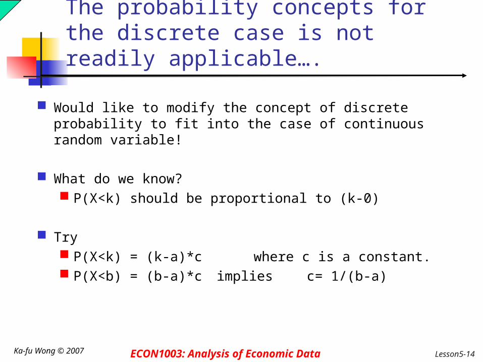
The probability concepts for the discrete case is not readily applicable….
Would like to modify the concept of discrete probability to fit into the case of continuous random variable!
What do we know? P(X<k) should be proportional to (k-0)
Try P(X<k) = (k-a)*c where c is a constant. P(X<b) = (b-a)*c implies c= 1/(b-a)

Lesson5-15 Ka-fu Wong © 2007 ECON1003: Analysis of Economic Data
The probability concepts for the discrete case is not readily applicable….
What is the probability that a dart randomly thrown will end up exactly in segment A (which lies on a straight line)?Suppose the dart has equal chance to land on any point of the line.
A
0.5 = (b-a)/2 * c = 1/2.
a b1/2
C=1/(b-a)
c is called the probability density.
Probability is simply the area
Lesson5-16 Ka-fu Wong © 2007 ECON1003: Analysis of Economic Data
The probability concepts for the discrete case is not readily applicable….
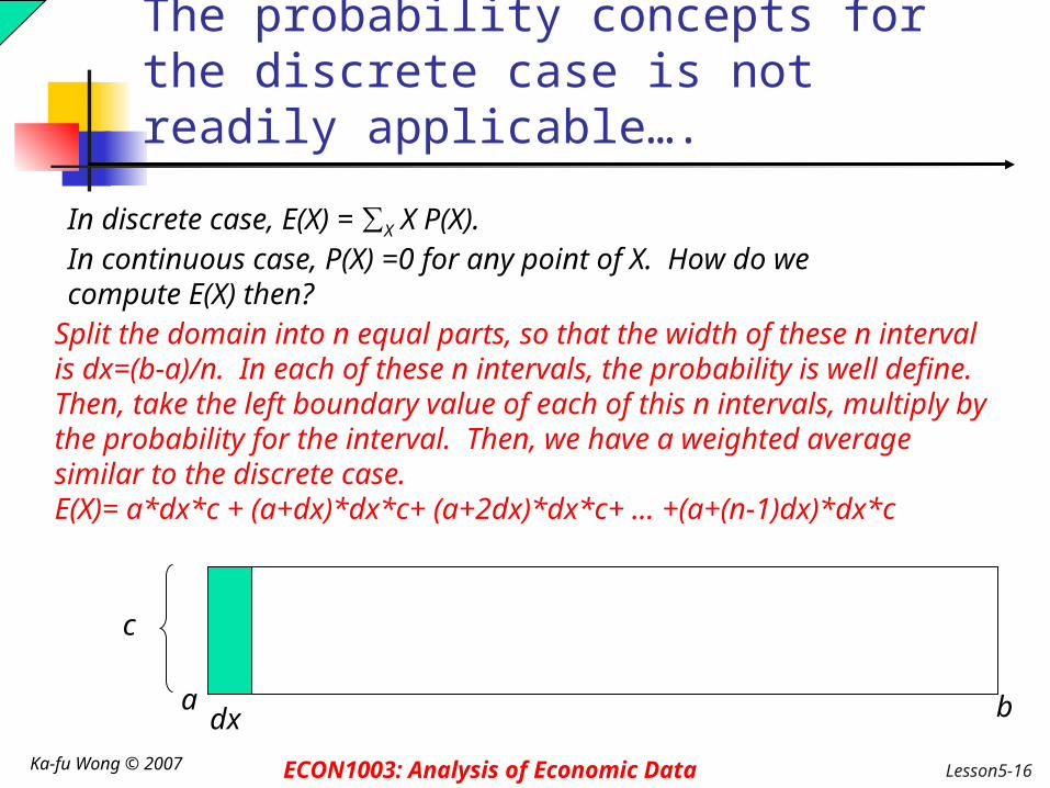
In discrete case, E(X) = ∑X X P(X).In continuous case, P(X) =0 for any point of X. How do we compute E(X) then?
Split the domain into n equal parts, so that the width of these n interval is dx=(b-a)/n. In each of these n intervals, the probability is well define. Then, take the left boundary value of each of this n intervals, multiply by the probability for the interval. Then, we have a weighted average similar to the discrete case.E(X)= a*dx*c + (a+dx)*dx*c+ (a+2dx)*dx*c+ … +(a+(n-1)dx)*dx*c
a b
c
dx

Lesson5-17 Ka-fu Wong © 2007 ECON1003: Analysis of Economic Data
The probability concepts for the discrete case is not readily applicable….
E(X)= a*dx*c + (a+dx)*dx*c+ (a+2dx)*dx*c+ … +(a+(n-1)dx)*dx*c
a b
c
dx
However, it is an approximation because a is only an approximate of the points within the interval (a, a+dx). Approximation improves if dx is made smaller, or n larger. That is, when dx is very very very closed to zero (but still positive), E(X)= limn-> [a*dx*c + (a+dx)*dx*c +… +(a+(n-1)dx)*dx*c]= limn-> ∑i [xi*dx*c ]=limdx->0 ∑i [xi*dx*c ]
][b
a
cdxxE(X)
xi xi+dx

Lesson5-18 Ka-fu Wong © 2007 ECON1003: Analysis of Economic Data
The probability concepts for the discrete case is not readily applicable….
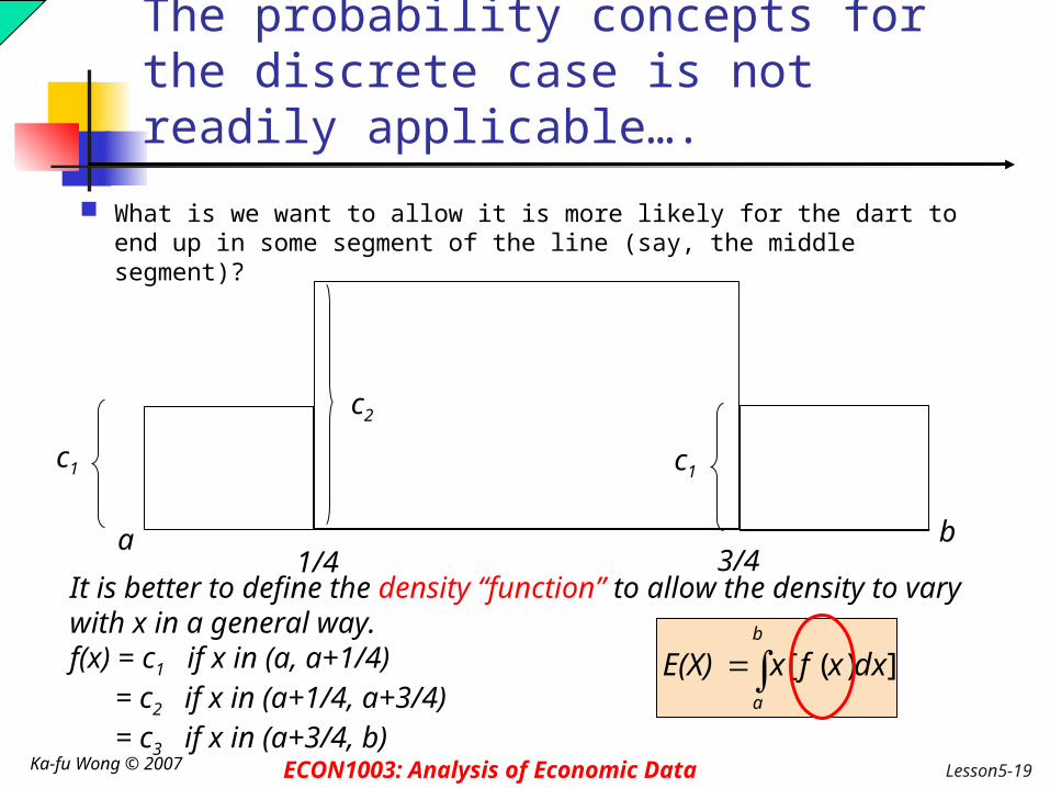
What if we want to allow it more likely for the dart to end up in some segment of the line (say, the middle segment)?
a b
c2
c1 c1
1/4 3/4
We can do it as long as we have the areas added up to 1: ¼*c1 + ½*c2 + ¼*c1 = 1.
Lesson5-19 Ka-fu Wong © 2007 ECON1003: Analysis of Economic Data
The probability concepts for the discrete case is not readily applicable….
What is we want to allow it is more likely for the dart to end up in some segment of the line (say, the middle segment)?
a b
c2
c1 c1
1/4 3/4It is better to define the density “function” to allow the density to vary with x in a general way. f(x) = c1 if x in (a, a+1/4) = c2 if x in (a+1/4, a+3/4) = c3 if x in (a+3/4, b)
])([b
a
dxxfxE(X)

Lesson5-20 Ka-fu Wong © 2007 ECON1003: Analysis of Economic Data
c d x
f(x)
Shaded area under the curve is the probability that X is between c and d
Probability as an area
d
c
f(x)dxdxcP )(
xf(x)dxXE )(

Lesson5-21 Ka-fu Wong © 2007 ECON1003: Analysis of Economic Data
Probability Density Function
The cumulative density function F(x0) is the area under the probability density function f(x) from the minimum x value (a) up to x0
00
0
xx
a
f(x)dxf(x)dx)F(x

Lesson5-22 Ka-fu Wong © 2007 ECON1003: Analysis of Economic Data
Expectations for Continuous Random Variables
The mean of X, denoted μX , is defined as the expected value of X
The variance of X, denoted σX2 , is defined as the
expectation of the squared deviation, (X - μX)2, of a random variable from its mean
-
X xf(x)dx E(X) μ
f(x)dx)μ(x])μE[(Xσ XXX222

Lesson5-23 Ka-fu Wong © 2007 ECON1003: Analysis of Economic Data
Linear Functions of Variables Let W = a + bX , where X has mean μX and variance
σX2 , and a and b are constants
Then the mean of W isE(W) = E(a+bX) = a + bE(X) = a + b μX
the variance isVar(W) = Var(a+bX) = b2Var(X) = b2σX
2
the standard deviation of W is|b|σX

Lesson5-24 Ka-fu Wong © 2007 ECON1003: Analysis of Economic Data
An important special case of the previous results is the standardized random variable
Z =( X- μX ) /σX
which has a mean 0 and variance 1
Linear Functions of Variables

Lesson5-25 Ka-fu Wong © 2007 ECON1003: Analysis of Economic Data
The Univariate Uniform Distribution
If c and d are numbers on the real line, the random variable X ~ U(c,d), i.e., has a univariate uniform distribution if
otherwise 0
dxcfor c-d
1=f(x)
The mean and standard deviation of a uniform random variable x are
122
cdand
dcXX

Lesson5-26 Ka-fu Wong © 2007 ECON1003: Analysis of Economic Data
The Uniform Density

Lesson5-27 Ka-fu Wong © 2007 ECON1003: Analysis of Economic Data
8 10 12 14 16 18 20 22
Learning exercise 4: Part-time Work on Campus
A student has been offered part-time work in a laboratory. The professor says that the work will vary from week to week. The number of hours will be between 10 and 20 with a uniform probability density function, represented as follows:
How tall is the rectangle? What is the probability of
getting less than 15 hours in a week?
Given that the student gets at least 15 hours in a week, what is the probability that more than 17.5 hours will be available?

Lesson5-28 Ka-fu Wong © 2007 ECON1003: Analysis of Economic Data
8 10 12 14 16 18 20 22
Learning exercise 4: Part-time Work on Campus
How tall is the rectangle? (20-10)*h = 1 h=0.1
What is the probability of getting less than 15 hours in a week? 0.1*(15-10) = 0.5
Given that the student gets at least 15 hours in a week, what is the probability that more than 17.5 hours will be available? 0.1*(20-17.5) = 0.25 0.25/0.5 = 0.5P(hour>17.5)/P(hour>15)
Lesson5-29 Ka-fu Wong © 2007 ECON1003: Analysis of Economic Data
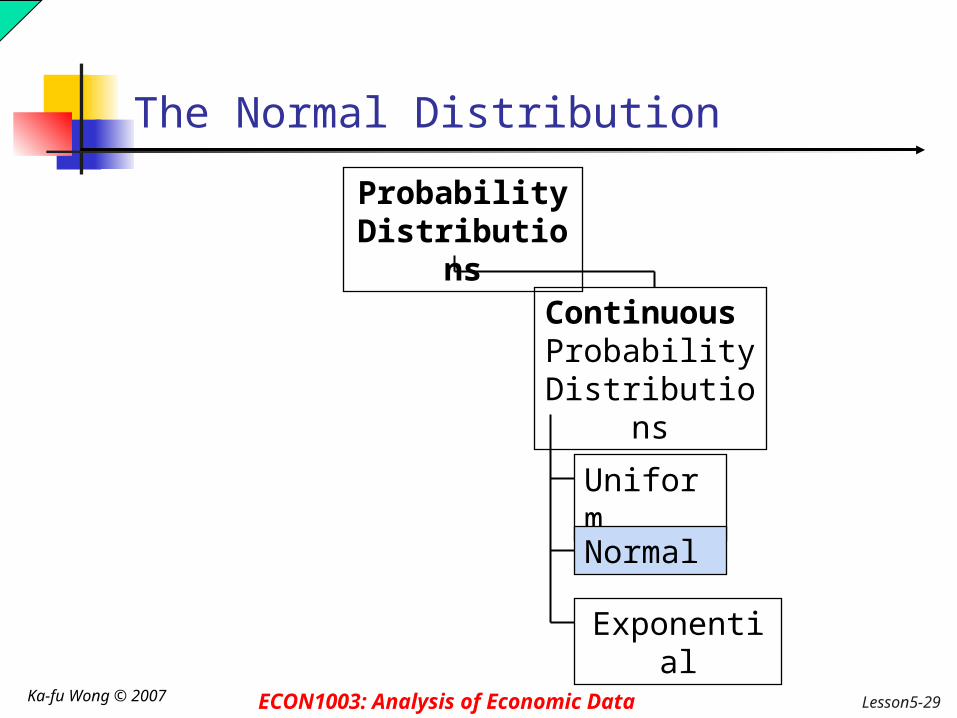
The Normal Distribution
Continuous Probability
Distributions
Probability Distributions
Uniform
Normal
Exponential

Lesson5-30 Ka-fu Wong © 2007 ECON1003: Analysis of Economic Data
‘ Bell Shaped’ Symmetrical Mean, Median and Mode
are Equal
Location is determined by the mean, μ
Spread is determined by the standard deviation, σ
The random variable has an infinite theoretical range: + to
Mean = Median = Mode
x
f(x)
μ
σ
Normal Distribution N(,2)
The normal probability distribution is asymptotic. That is the curve gets closer and closer to the X-axis but never actually touches it.

Lesson5-31 Ka-fu Wong © 2007 ECON1003: Analysis of Economic Data
The Normal Distribution N(,2)
The normal distribution closely approximates the probability distributions of a wide range of random variables
Distributions of sample means approach a normal distribution given a “large” sample size
Computations of probabilities are direct and elegant
The normal probability distribution has led to good business decisions for a number of applications
Sum of normal random variables remain normal.
Normal distribution is completely characterized by two parameters, mean and variance.

Lesson5-32 Ka-fu Wong © 2007 ECON1003: Analysis of Economic Data
N(,2)
x
x
x
(a)
(b)
(c)
Changing shifts the location of the distribution.Changing 2 changes the dispersion.

Lesson5-33 Ka-fu Wong © 2007 ECON1003: Analysis of Economic Data
The Normal Probability Distribution
The random variable X ~ N(,2), i.e., has a univariate normal distribution if for all x on the real line (-,+ )
e2
1=f(x)
2-x
21
-
and are the mean and standard deviation, = 3.14159 … and e = 2.71828 is the base of natural or Naperian logarithms.

Lesson5-34 Ka-fu Wong © 2007 ECON1003: Analysis of Economic Data
Normal Distribution Probability
Probability is the area under the curve!
c dX
f(X) A table may be constructed to help us find the probability

Lesson5-35 Ka-fu Wong © 2007 ECON1003: Analysis of Economic Data
Moments of Standard Normal Random Variables N(0, )
Mean=0 Variance =1 Skewness = 0 Kurtosis = 3 Excess kurtosis =0

Lesson5-36 Ka-fu Wong © 2007 ECON1003: Analysis of Economic Data
Infinite Number of Normal Distribution Tables
Normal distributions differ by mean & standard deviation.
Each distribution would require its own table.
X
f(X)

Ka-fu Wong © 2007 ECON1003: Analysis of Economic Data
The Standard Normal Probability Distribution -- N(0,1)
The standard normal distribution is a normal distribution with a mean of 0 and a standard deviation of 1.
It is also called the z distribution.
A z-value is the distance between a selected value, designated X, and the population mean , divided by the population standard deviation, . The formula is:
X
Z
0])([1
)(1
)(
XEXE
XEZE
1)(1
)(1
)(22
XVarXVarX
VarZVar

Ka-fu Wong © 2007 ECON1003: Analysis of Economic Data
The Standard Normal Probability Distribution
Any normal random variable can be transformed to a standard normal random variable
Suppose X ~ N(µ, 2) Z=(X-µ)/ ~ N(0,1)
P(X<k) = P [(X-µ)/ < (k-µ)/ ]

Lesson5-39 Ka-fu Wong © 2007 ECON1003: Analysis of Economic Data
Standardize the Normal Distribution
0
= 1
Z
Because we can transform any normal random variable into standard normal random variable, we need only one table!
Normal Distribution
Standardized Normal Distribution
X
XZ

Lesson5-40 Ka-fu Wong © 2007 ECON1003: Analysis of Economic Data
Standardizing Example
Z 0 .12
Normal distribution N(5,100)= 5, = 10
Standardized Normal Distribution N(0,1) = 0, = 1
X5 6.2
12.010
52.6
XZ
010
55
XZ

Lesson5-41 Ka-fu Wong © 2007 ECON1003: Analysis of Economic Data
Obtaining the Probability
Z0
= 1
0.12
Z .00 .01
0.0 .0000 .0040 .0080
.0398 .0438
0.2 .0793 .0832 .0871
0.3 .1179 .1217 .1255
0.0478
.02
0.1 .0478
Standardized Normal Probability Table (Portion)
ProbabilitiesShaded Area Exaggerated

Lesson5-42 Ka-fu Wong © 2007 ECON1003: Analysis of Economic Data
Example P(3.8 X 5)
Z0-0.12
Normal Distribution
0.0478
Standardized Normal Distribution
Shaded Area Exaggerated
X = 5
= 10
3.8
12.010
58.3
XZ

Lesson5-43 Ka-fu Wong © 2007 ECON1003: Analysis of Economic Data
Example (2.9 X 7.1)
0-.21 Z.21
Normal Distribution
.1664
.0832.0832
Standardized Normal Distribution
5
= 10
2.9 7.1 X
Shaded Area Exaggerated
21.010
59.2
XZ
21.010
51.7
XZ
Lesson5-44 Ka-fu Wong © 2007 ECON1003: Analysis of Economic Data
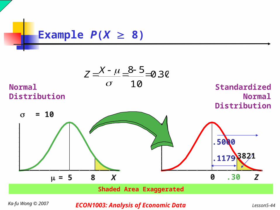
Example P(X 8)
Z0 .30
Normal Distribution
Standardized Normal Distribution
.1179
.5000 .3821
X = 5
= 10
8
Shaded Area Exaggerated
30.010
58
XZ

Lesson5-45 Ka-fu Wong © 2007 ECON1003: Analysis of Economic Data
Example P(7.1 X 8)
0 .30 Z.21
Normal Distribution
.0832
.1179 .0347
Standardized Normal Distribution
= 5
= 10
87.1 XShaded Area Exaggerated
21.010
51.7
XZ
3.010
58
XZ

Lesson5-46 Ka-fu Wong © 2007 ECON1003: Analysis of Economic Data
Normal Distribution Thinking Challenge
You work in Quality Control for GE. Light bulb life has a normal distribution with µ= 2000 hours & = 200 hours. What’s the probability that a bulb will last between 2000 & 2400 hours? less than 1470 hours?

Lesson5-47 Ka-fu Wong © 2007 ECON1003: Analysis of Economic Data
Solution P(2000 X 2400)
Z0 2.0
Normal Distribution
.4772
Standardized Normal Distribution
X = 2000
= 200
2400
P(2000<X<2400) = P [(2000-µ)/ <(X-µ)/ < (2400-µ)/ ]= P[(X-µ)/ < (2400-µ)/ ] – P [(X-µ)/ < (2000-µ)/ ]= P[(X-µ)/ < (2400-µ)/ ] – 0.5
Shaded Area Exaggerated
2.0200
20002400
σμXZ

Lesson5-48 Ka-fu Wong © 2007 ECON1003: Analysis of Economic Data
Solution P(X 1470)
Z 0-2.65
Normal Distribution
.4960 .0040
.5000
Standardized Normal Distribution
X = 2000
= 200
1470
P(X<1470) = P [(X-µ)/ < (1470-µ)/ ]
Shaded Area Exaggerated
2.65200
20004701
σμXZ

Lesson5-49 Ka-fu Wong © 2007 ECON1003: Analysis of Economic Data
Finding Z Values for Known Probabilities
Z .00 .02
0.0 .0000 .0040 .0080
0.1 .0398 .0438 .0478
0.2 .0793 .0832 .0871
.1179 .1255
Z Z = 0
Z = 1
.31
.1217.01
0.3 .1217
Standardized Normal Probability Table (Portion)
What Is Z Given P(Z) = 0.1217?
Shaded Area Exaggerated

Lesson5-50 Ka-fu Wong © 2007 ECON1003: Analysis of Economic Data
Finding X Values for Known Probabilities
Z Z = 0
Z = 1
.31X = 5
= 10
?
Normal Distribution Standardized Normal Distribution
.1217 .1217
1.810)31.0(5 ZXShaded Area Exaggerated

Lesson5-51 Ka-fu Wong © 2007 ECON1003: Analysis of Economic Data
EXAMPLE 1
The bi-monthly starting salaries of recent MBA graduates follows the normal distribution with a mean of $20,000 and a standard deviation of $2,000. What is the z-value for a salary of $24,000?
00.22000$
000,20$000,24$
X
z

Lesson5-52 Ka-fu Wong © 2007 ECON1003: Analysis of Economic Data
EXAMPLE 1 continued
A z-value of 2 indicates that the value of $24,000 is 2 standard deviation above the mean of $20,000.
A z-value of –1.50 indicates that $17,000 is 1.5 standard deviation below the mean of $20,000.
50.12000$
000,20$000,17$
X
z
What is the z-value of $17,000 ?

Lesson5-53 Ka-fu Wong © 2007 ECON1003: Analysis of Economic Data
Areas Under the Normal Curve
About 68 percent of the area under the normal curve is within one standard deviation of the mean.
± P( - < X < + ) = 0.6826
About 95 percent is within two standard deviations of the mean. ± 2 P( - 2 < X < + 2 ) = 0.9544
Practically all is within three standard deviations of the mean. ± 3 P( - 3 < X < + 3 ) = 0.9974

Lesson5-54 Ka-fu Wong © 2007 ECON1003: Analysis of Economic Data
EXAMPLE 2
The daily water usage per person in New Providence, New Jersey is normally distributed with a mean of 20 gallons and a standard deviation of 5 gallons.
About 68 percent of those living in New Providence will use how many gallons of water?
About 68% of the daily water usage will lie between 15 and 25 gallons.

Lesson5-55 Ka-fu Wong © 2007 ECON1003: Analysis of Economic Data
EXAMPLE 2 continued
What is the probability that a person from New Providence selected at random will use between 20 and 24 gallons per day?
00.05
2020
X
z
80.05
2024
X
z
P(20<X<24)=P[(20-20)/5 < (X-20)/5 < (24-20)/5 ] =P[ 0<Z<0.8 ]
The area under a normal curve between a z-value of 0 and a z-value of 0.80 is 0.2881. We conclude that 28.81 percent of the residents use between 20 and 24 gallons of water per day.

Lesson5-56 Ka-fu Wong © 2007 ECON1003: Analysis of Economic Data
How do we find P(0<z<0.8)
P(0<z<0.8) = P(z<0.8) – P(z<0)=0.7881 – 0.5=0.2881
P(z<c)
c
P(0<z<c)
c0
P(0<z<0.8) = 0.2881

Lesson5-57 Ka-fu Wong © 2007 ECON1003: Analysis of Economic Data
EXAMPLE 2 continued
What percent of the population use between 18 and 26 gallons of water per day?
40.05
2018
X
z
20.15
2026
X
z
Suppose X ~ N(µ, 2) Z=(X-µ)/ ~ N(0,1)
P(X<k) = P [(X-µ)/ < (k-µ)/ ]

Lesson5-58 Ka-fu Wong © 2007 ECON1003: Analysis of Economic Data
How do we find P(-0.4<z<1.2)
P(z<c)
c
P(0<z<c)
c0
P(-0.4<z<1.2) = P(-0.4<z<0) + P(0<z<1.2)=P(0<z<0.4) + P(0<z<1.2)=0.1554+0.3849=0.5403
P(-0.4<z<1.2) = P(z<1.2) - P(z<-0.4)= P(z<1.2) - P(z>0.4) = P(z<1.2) – [1- P(z<0.4)]=0.8849 – [1- 0.6554]=0.5403
P(-0.4<z<0) =P(0<z<0.4) because of symmetry of the z distribution.

Lesson5-59 Ka-fu Wong © 2007 ECON1003: Analysis of Economic Data
Steps to find the X value for a known probability:1. Find the Z value for the known probability2. Convert to X units using the formula:
Finding the X value for a Known Probability
ZσμX

Lesson5-60 Ka-fu Wong © 2007 ECON1003: Analysis of Economic Data
Finding the X value for a Known Probability
Example: Suppose X is normal with mean 8.0 and standard
deviation 5.0. Now find the X value so that only 20% of all values are
below this X
X? 8.0
.20
Z? 0

Lesson5-61 Ka-fu Wong © 2007 ECON1003: Analysis of Economic Data
Find the Z value for 20% in the Lower Tail
20% area in the lower tail is consistent with a Z value of -0.84
Standardized Normal Probability Table (Portion)
X? 8.0
.20
Z-0.84 0
1. Find the Z value for the known probability
z F(z)
.82 .7939
.83 .7967
.84 .7995
.85 .8023
.80

Lesson5-62 Ka-fu Wong © 2007 ECON1003: Analysis of Economic Data
2. Convert to X units using the formula:
Finding the X value
803
0584008
.
.).(.
ZσμX
So 20% of the values from a distribution with mean 8.0 and standard deviation 5.0 are less than 3.80

Lesson5-63 Ka-fu Wong © 2007 ECON1003: Analysis of Economic Data
EXAMPLE 3
Professor Mann has determined that the scores in his statistics course are approximately normally distributed with a mean of 72 and a standard deviation of 5. He announces to the class that the top 15 percent of the scores will earn an A.
What is the lowest score a student can earn and still receive an A?

Lesson5-64 Ka-fu Wong © 2007 ECON1003: Analysis of Economic Data
Example 3 continued
To begin let k be the score that separates an A from a B. 15 percent of the students score more than k, then 35 percent
must score between the mean of 72 and k. Write down the relation between k and the probability:
P(X>k) = 0.15 and P(X<k) =1-P(X>k) = 0.85 Transform X into z:
P[(X-72)/5) < (k-72)/5 ] = P[z < (k-72)/5] P[0<z < s] =0.85 -0.5 = 0.35
X72 k
Z0 ?
0.150.35

Lesson5-65 Ka-fu Wong © 2007 ECON1003: Analysis of Economic Data
Example 3 continued
Find s from table: P[0<z<1.04]=0.35
Compute k: (k-72)/5=1.04 implies K=77.2
Those with a score of 77.2 or more earn an A.
X72 77.2
Z0 1.04
0.150.35

Lesson5-66 Ka-fu Wong © 2007 ECON1003: Analysis of Economic Data
How do we know that the data are likely drawn from normal?
1. Check the moments Skewness =0 Excess Kurtosis = 0
(For instance, refer to section 16.7 “Tests for Skewness and Excess Kurtosis”, p.567 of Estimation and Inference in Econometrics by Davidson and MacKinnon)
2. Normal probability plot1. Suppose we have n observations in the sample.
Sort them in ascending order. Compute the empirical z value (i.e., (x-mx)/sx)
2. Generate a column 0.5, 1.5, …..,[ 0.5+(n-1)]. Call this column U.3. Generate another column p(z) = U/n. 4. Generate another column theoretical z = NORMSINV(p(z))5. Plot empirical z against the theoretical z.6. If the data has normal distribution, the plot should be a straight
line.

Lesson5-67 Ka-fu Wong © 2007 ECON1003: Analysis of Economic Data
Normal Probability Plot (The data are generated from a normal distribution.)
-3.5
-3
-2.5
-2
-1.5
-1
-0.5
0
0.5
1
1.5
2
2.5
3
3.5
-3.5 -3 -2.5 -2 -1.5 -1 -0.5 0 0.5 1 1.5 2 2.5 3 3.5
Theoretical z value
z valu
e from
data

Lesson5-68 Ka-fu Wong © 2007 ECON1003: Analysis of Economic Data
Normal Probability Plot (The data are generated from a uniform distribution.)
-3.5
-3
-2.5
-2
-1.5
-1
-0.5
0
0.5
1
1.5
2
2.5
3
3.5
-3.5 -3 -2.5 -2 -1.5 -1 -0.5 0 0.5 1 1.5 2 2.5 3 3.5
Theoretical z value
z valu
e from
data

Lesson5-69 Ka-fu Wong © 2007 ECON1003: Analysis of Economic Data
The Normal Approximation to the Binomial
The normal distribution (a continuous distribution) yields a good approximation of the binomial distribution (a discrete distribution) for large values of n (number of trials).
The normal probability distribution is generally a good approximation to the binomial probability distribution when n and n(1- ) are both greater than 5.
Why can we approximate binomial by normal?Because of the Central Limit Theorem.

Lesson5-70 Ka-fu Wong © 2007 ECON1003: Analysis of Economic Data
Normal Distribution Approximation for Binomial Distribution
Recall the binomial distribution: n independent trials probability of success on any given trial = P
Random variable X: Xi =1 if the ith trial is “success”
Xi =0 if the ith trial is “failure”
nPμE(X)
P)nP(1-σVar(X) 2

Lesson5-71 Ka-fu Wong © 2007 ECON1003: Analysis of Economic Data
Normal Distribution Approximation for Binomial Distribution
The shape of the binomial distribution is approximately normal if n is large
The normal is a good approximation to the binomial when nP(1 – P) > 9
Standardize to Z from a binomial distribution:
P)nP(1
npX
Var(X)
E(X)XZ
Lesson5-72 Ka-fu Wong © 2007 ECON1003: Analysis of Economic Data
Normal Distribution Approximation for Binomial Distribution
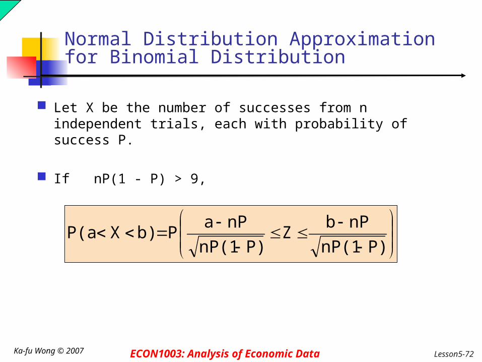
Let X be the number of successes from n independent trials, each with probability of success P.
If nP(1 - P) > 9,
P)nP(1
nPbZ
P)nP(1
nPaPb)XP(a

Lesson5-73 Ka-fu Wong © 2007 ECON1003: Analysis of Economic Data
Binomial Approximation Example
40% of all voters support ballot proposition A. What is the probability that between 76 and 80 voters indicate support in a sample of n = 200 ?
E(X) = µ = nP = 200(0.40) = 80 Var(X) = σ2 = nP(1 – P) = 200(0.40)(1 – 0.40) = 48
( note: nP(1 – P) = 48 > 9 )
0.21900.28100.5000
0.58)F(F(0)
0)Z0.58P(
0.4)200(0.4)(1
8080Z
0.4)200(0.4)(1
8076P80)XP(76

Lesson5-74 Ka-fu Wong © 2007 ECON1003: Analysis of Economic Data
The Exponential Distribution
Used to model the length of time between two occurrences of an event (the time between arrivals)
Examples: Time between trucks arriving at an unloading dockTime between transactions at an ATM MachineTime between phone calls to the main operator

Lesson5-75 Ka-fu Wong © 2007 ECON1003: Analysis of Economic Data
The Exponential Distribution
The exponential random variable T (t>0) has a probability density function
Where is the mean number of occurrences per unit time t is the length of time until the next occurrence e = 2.71828
T is said to follow an exponential probability distribution
0 for t λef(t) λt

Lesson5-76 Ka-fu Wong © 2007 ECON1003: Analysis of Economic Data
The Exponential Distribution
λteF(t) 1
Defined by a single parameter, its mean (lambda)
The cumulative distribution function (the probability that an arrival time is less than some specified time t) is
where e = mathematical constant approximated by 2.71828
= the population mean number of arrivals per unit
t = any value of the continuous variable where t > 0

Lesson5-77 Ka-fu Wong © 2007 ECON1003: Analysis of Economic Data
Exponential Distribution Example
Example: Customers arrive at the service counter at the rate of 15 per hour. What is the probability that the arrival time between consecutive customers is less than three minutes?
The mean number of arrivals per hour is 15, so = 15
Three minutes is .05 hours
P(arrival time < .05) = 1 – e- X = 1 – e-(15)(.05) = 0.5276
So there is a 52.76% probability that the arrival time between successive customers is less than three minutes

Lesson5-78 Ka-fu Wong © 2007 ECON1003: Analysis of Economic Data
Joint Cumulative Distribution Functions
Let X1, X2, . . .Xk be continuous random variables
Their joint cumulative distribution function, F(x1, x2, . . .xk)
defines the probability that simultaneously X1 is less than x1, X2 is less than x2, and so on; that is
)xX,...,xX,xP(X)x,...,x,F(x kk2211k21

Lesson5-79 Ka-fu Wong © 2007 ECON1003: Analysis of Economic Data
Joint Cumulative Distribution Functions
The cumulative distribution functions F(x1), F(x2), . . .,F(xk)
of the individual random variables are called their marginal distribution functions
The random variables are independent if and only if
)F(x...))F(xF(x)x,...,x,F(x k21k21

Lesson5-80 Ka-fu Wong © 2007 ECON1003: Analysis of Economic Data
Features of a Bivariate Continuous Distribution
Let X1 and X2 be a random variables that takes any real values in a region (rectangle) of (a,b,c,d). The number of possible outcomes are by definition infinite.
The main features of a probability density function f(x1,x2) are:
f(x1,x2) 0 for all (x1,x2) and may be larger than 1.
The probability that (X1,X2) falls into a region (rectangle) or (p,q,r,s) is
and lies between 0 and 1. P((X1,X2) (a,b,c,d)) = 1.
P((X1,X2) = (x1,x2) ) = 0.
q
p
s
r
dxdxxxfsrqpXXP 212121 ),()),,,(),((

Lesson5-81 Ka-fu Wong © 2007 ECON1003: Analysis of Economic Data
The Bivariate Uniform Distribution
If a, b, c and d are numbers on the real line, , the random variable (X1,X2) ~ U(a,b,c,d), i.e., has a bivariate uniform distribution if
otherwise 0
dxc and bxa for c)-a)(d-(b
1
=)x,f(x 2121

Lesson5-82 Ka-fu Wong © 2007 ECON1003: Analysis of Economic Data
The Marginal Density
The marginal density functions are:
f(x,y)dx f(y)
f(x,y)dy f(x)

Lesson5-83 Ka-fu Wong © 2007 ECON1003: Analysis of Economic Data
The Conditional Density
The conditional density functions are:
y) f(x,y)/f(f(x|y)
x) f(x,y)/f(f(y|x)

Lesson5-84 Ka-fu Wong © 2007 ECON1003: Analysis of Economic Data
The Expectation (Mean) of Continuous Probability Distribution
For univariate probability distribution, the expectation or mean E(X) is computed by the formula:
For bivariate probability distribution, the the expectation or mean E(X) is computed by the formula:
xf(x)dxE(X)
dyxf(x,y)dx E(X)

Lesson5-85 Ka-fu Wong © 2007 ECON1003: Analysis of Economic Data
Conditional Mean of Bivariate Discrete Probability Distribution
For bivariate probability distribution, the conditional expectation or conditional mean E(X|Y) is computed by the formula:
Unconditional expectation or mean of X, E(X)
dxxf(x|y)y)E(X|Y
]E[μ
E[E(X|Y)]
dx f(y)dyxf(x|y) E(X)
X

Lesson5-86 Ka-fu Wong © 2007 ECON1003: Analysis of Economic Data
Expectation of a linear transformed random variable
If a and b are constants and X is a random variable, then E(a) = aE(bX) = bE(X)E(a+bX) = a+bE(X)
bE(x)a
x f(x) dxbf(x) dxa
bx f(x) dxa f(x) dx
xbx) f(x) d(a
bx) dxbx) f(a(abx)E(a

Lesson5-87 Ka-fu Wong © 2007 ECON1003: Analysis of Economic Data
The Variance of a Continuous Probability Distribution
For univariate continuous probability distribution
-
f(x)dxμ)(X ] μ)E[(XVar(X) 22
If a and b are constants and X is a random variable, then Var(a) = 0Var(bX) = b2Var(X)Var(a+bX) = b2Var(X)

Lesson5-88 Ka-fu Wong © 2007 ECON1003: Analysis of Economic Data
The Covariance of a Bivariate Discrete Probability Distribution
dxdyyx)fμ)(Yμ(X)]μ)(YμE[(XCov(X,Y) YXYX ),(
Covariance measures how two random variables co-vary.
If a and b are constants and X is a random variable, then Cov(a,b) = 0Cov(a,bX) = 0Cov(a+bX,Y) = bCov(X,Y)

Lesson5-89 Ka-fu Wong © 2007 ECON1003: Analysis of Economic Data
Correlation coefficient
The strength of the dependence between X and Y is measured by the correlation coefficient:
Y)Var(X)Var(
Cov(X,Y)Corr(X,Y)

Lesson5-90 Ka-fu Wong © 2007 ECON1003: Analysis of Economic Data
Variance of a sum of random variables
If a and b are constants and X and Y are random variables, then
Var(X+Y) = Var(X) + Var(Y) + 2Cov(X,Y)
Cov(X,Y)Var(Y)Var(X)
)]μ)(YμE[(X)μE[(Y] )μ E[ (X
)]μ)(Yμ(X)μ(Y )μE[ (X
)]μ(Y)μE[ (X
) ]μ (μYE[ XY)Var(X
YXYX
YXYX
YX
YX
2
2
22
2
2
2
2
2

Lesson5-91 Ka-fu Wong © 2007 ECON1003: Analysis of Economic Data
Variance of a sum of random variables
If a and b are constants and X and Y are random variables, then
Var(aX+bY) =a2Var(X) + b2Var(Y) + 2abCov(X,Y)
abCov(X,Y)Var(Y)bVar(X)a
)]μ)(YμabE[(X)μE[(Yb] )μE[ (X a
)]bμ)(bYaμ(aX)μ(Yb )μ(XE[ a
)]bμ(bY)aμE[ (aX
) ]bμ (aμbYE[ aXbY)Var(aX
YXYX
YXYX
YX
YX
2
2
2
22
222
222
2
2
2
2

Lesson5-92 Ka-fu Wong © 2007 ECON1003: Analysis of Economic Data
Sums of Random Variables
Let X1, X2, . . .Xk be k random variables with
means μ1, μ2,. . . μk and
variances σ12, σ2
2,. . ., σk2.
Then, the mean of their sum is the sum of their means
kk μμμ)XXE(X ...... 2121

Lesson5-93 Ka-fu Wong © 2007 ECON1003: Analysis of Economic Data
Sums of Random Variables Let X1, X2, . . .Xk be k random variables with
means μ1, μ2,. . . μk and variances σ1
2, σ22,. . ., σk
2.
Then:
If the covariance between every pair of these random variables is 0, then the variance of their sum is the sum of their variances
However, if the covariances between pairs of random variables are not 0, the variance of their sum is
2k
22
21k21 σ...σσ)X...XVar(X
)X,Cov(X2σ...σσ)X...XVar(X j
1K
1i
K
1iji
2k
22
21k21

Lesson5-94 Ka-fu Wong © 2007 ECON1003: Analysis of Economic Data
Differences Between Two Random Variables
For two random variables, X and Y
The mean of their difference is the difference of their means; that is
If the covariance between X and Y is 0, then the variance of their difference is
If the covariance between X and Y is not 0, then the variance of their difference is
YX μμY)E(X
2Y
2X σσY)Var(X
Y)2Cov(X,σσY)Var(X 2Y
2X

Lesson5-95 Ka-fu Wong © 2007 ECON1003: Analysis of Economic Data
Linear Combinations of Random Variables
A linear combination of two random variables, X and Y, (where a and b are constants) is
The mean of W is
bYaXW
YXW bμaμbY]E[aXE[W]μ

Lesson5-96 Ka-fu Wong © 2007 ECON1003: Analysis of Economic Data
Linear Combinations of Random Variables
The variance of W is
Or using the correlation,
If both X and Y are joint normally distributed random variables then the linear combination, W, is also normally distributed
Y)2abCov(X,σbσaσ 2Y
22X
22W
YX2Y
22X
22W σY)σ2abCorr(X,σbσaσ

Lesson5-97 Ka-fu Wong © 2007 ECON1003: Analysis of Economic Data
Example
Two tasks must be performed by the same worker.
X = minutes to complete task 1; μx = 20, σx = 5
Y = minutes to complete task 2; μy = 20, σy = 5
X and Y are normally distributed and independent
What is the mean and standard deviation of the time to complete both tasks?

Lesson5-98 Ka-fu Wong © 2007 ECON1003: Analysis of Economic Data
Example
X = minutes to complete task 1; μx = 20, σx = 5
Y = minutes to complete task 2; μy = 30, σy = 8
What are the mean and standard deviation for the time to complete both tasks?
Since X and Y are independent, Cov(X,Y) = 0, so
The standard deviation is
YXW
503020μμμ YXW
89(8)(5) Y)2Cov(X,σσσ 222Y
2X
2W
9.43489σW

Lesson5-99 Ka-fu Wong © 2007 ECON1003: Analysis of Economic Data
- END -
Lesson 5: Lesson 5: Continuous Probability Distributions