Embed Size (px)
Citation preview
Mon. Not. R. Astron. Soc. 000, ??–?? (2002) Printed 6 January 2016 (MN LATEX style file v2.2)
K2 Variable Catalogue II: Machine Learning Classificationof Variable Stars and Eclipsing Binaries in K2 Fields 0-4
D. J. Armstrong1,2?, J. Kirk1, K. W. F. Lam1, J. McCormac1, H. P. Osborn1, J.Spake1,3, S. Walker1, D. J. A. Brown1, M. H. Kristiansen4, D. Pollacco1, R. West1,P. J. Wheatley1
1University of Warwick, Department of Physics, Gibbet Hill Road, Coventry, CV4 7AL, UK2ARC, School of Mathematics & Physics, Queen’s University Belfast, University Road, Belfast BT7 1NN, UK3Astrophysics Group, School of Physics, University of Exeter, Stocker Road, Exeter, EX4 4QL, UK4DTU Space, National Space Institute, Technical University of Denmark, Elektrovej 327, DK-2800 Lyngby, Denmark
Accepted . Received
ABSTRACTWe are entering an era of unprecedented quantities of data from current and plannedsurvey telescopes. To maximise the potential of such surveys, automated data analy-sis techniques are required. Here we implement a new methodology for variable starclassification, through the combination of Kohonen Self Organising Maps (SOM, anunsupervised machine learning algorithm) and the more common Random Forest (RF)supervised machine learning technique. We apply this method to data from the K2mission fields 0–4, finding 154 ab-type RR Lyraes (10 newly discovered), 377 δ Scutipulsators, 133 γ Doradus pulsators, 183 detached eclipsing binaries, 290 semi-detachedor contact eclipsing binaries and 9399 other periodic (mostly spot-modulated) sources,once class significance cuts are taken into account. We present lightcurve features forall K2 stellar targets, including their three strongest detected frequencies, which canbe used to study stellar rotation periods where the observed variability arises fromspot modulation. The resulting catalogue of variable stars, classes, and associated datafeatures are made available online. We publish our SOM code in Python as part of theopen source PyMVPA package, which in combination with already available RF modulescan be easily used to recreate the method.
Key words: stars: variable: general – catalogues – methods: data analysis – binaries:eclipsing – techniques: photometric
1 INTRODUCTION
Data flows from new and planned astronomical survey tele-scopes are steadily increasing. This shows no sign of stop-ping, with LSST starting operations in ∼2020. There isclearly a need for accurate, fast, automated classification ofphotometric lightcurves to maximise the scientific returnsfrom these surveys. Even when later spectroscopic followupis required, finding which targets to prioritise is a necessaryfirst step.
The literature contains multiple examples of such clas-sification, using a wide variety of techniques. These includea variety of supervised machine learning applications (e.g.Eyer & Blake 2005; Mahabal et al. 2008; Blomme et al. 2010;Debosscher et al. 2011; Brink et al. 2013; Nun et al. 2014).Recently Random Forests (RF) have begun to gain popu-
larity, due to their robustness and applicability to differentsets of data, extracted lightcurve properties, and classifica-tion schemes (e.g. Richards et al. 2011b, 2012; Masci et al.2014). Several improvements have been proposed, in areassuch as parametrising lightcurves with maximal informationretention (Kugler et al. 2015), and adjusting for training setdeficiencies (Richards et al. 2011a). One method of unsuper-vised machine learning is a Kohonen Self-Organising-Map(SOM, Kohonen 1990) demonstrated by Brett et al. (2004)in an astronomical context. Here we adopt a novel techniquebased on a combination of SOM and RF machine learning.SOMs can efficiently parametrise lightcurve shapes withoutresorting to specific lightcurve features, and RFs are capableof placing objects into classes.
In this work we apply these techniques to data from theK2 mission, the repurposed Kepler satellite (Borucki et al.2010). K2 and its predecessor Kepler have left a lasting markin studies of variable stars, showing that most δ Scuti and γ
c© 2002 RAS
arX
iv:1
512.
0124
6v2
[as
tro-
ph.S
R]
5 J
an 2
016

2 Armstrong et. al.
Dor stars show pulsations in both the p-mode and g-modefrequency regimes (Grigahcene et al. 2010). Many studieshave been performed on Kepler variable stars (e.g. Blommeet al. 2010; Balona et al. 2011; Balona & Dziembowski 2011;Debosscher et al. 2011; Uytterhoeven et al. 2011; Tkachenkoet al. 2013; Bradley et al. 2015), but few so far on K2. Balonaet al. (2015) studied B star variability in Kepler and K2, andfound that K2 data presented some new challenges from theoriginal mission. Despite these, it has for example discoveredthe several RR Lyrae stars known outside our own Galaxy(Molnar et al. 2015). LaCourse et al. (2015) have also pro-duced a catalogue of eclipsing binary stars in K2 field 0.
The initial version of this catalogue (Armstrong et al.2015) classified several thousand K2 variable stars in K2fields 0 and 1. This classification was based on an interpreta-tion of lightcurve periodicity, and split objects into Periodic,Quasiperiodic, and Aperiodic variables. Here we improve onthis initial work, by applying an automated technique toclassify variables into more usual classes. We extend theclassification to K2 fields 0–4, and will release updates asmore K2 fields become available.
2 DATA
2.1 Source
Data are taken from the K2 satellite (Howell et al. 2014). K2is the repurposed Kepler mission, and provides lightcurveflux measurements at a 30 minute ‘long’ cadence contin-uously for 80 days per target. Targets are organised intocampaigns, with each campaign spanning an ∼80 day pe-riod and covering several thousand objects. A much smallernumber of targets (a few tens per campaign) are availableat the ‘short’ cadence of ∼1 minutes. For the purposes ofthis work, we restrict ourselves to long cadence data only,to preserve uniformity in the data. At the time of writing,5 campaigns had been released to the public (covering fields0–4), with more due as the mission continues. Four of thesecampaigns cover ∼80 days, with the first campaign 0 cov-ering ∼40 days. We take data for these campaigns from theMichulski Archive for Space Telescopes (MAST) website1,limiting ourselves to objects classified as stars in the MASTcatalogue. This cut primarily removes a small number of so-lar system bodies and extended sources from the analysis.At this point, we have 68910 object lightcurves.
For the purposes of training the classifier, we also usedata from the original Kepler mission. In these cases a singlequarter of long cadence Kepler data is randomly selected.This covers ∼90 days, and hence is similar to a single K2campaign in duration and cadence. Kepler does howeverhave different noise properties than K2, particularly in re-gards to the ∼6 hour thruster firing, which is present inK2 but not in Kepler. Kepler data was also downloadedfrom MAST, and the Presearch-Data-Conditioning (PDC)detrended lightcurves (Stumpe et al. 2012; Smith et al. 2012)used.
1 https://archive.stsci.edu/k2/
Table 1. Times of pointing characteristic change, used to split
the K2 data before detrending
Campaign Split TimeBJD - 2454833
0 N/A1 2016.0
2 2101.41
3 N/A4 2273.0
2.2 Extraction and Detrending
K2 data shows instrumental artefacts not previously seenin the original Kepler mission. The strongest of these isa signal at ∼6 hours, which is the timescale on which thesatellite thrusters are fired to adjust the spacecraft point-ing. This pointing adjustment is necessary due to drift as-sociated with the new mode of operations, and is explainedfully in the K2 mission papers. It has the unfortunate ef-fect of causing systematic noise, due to aperture losses andinter-pixel sensitivity changes. A number of techniques havebeen put forward for removing this noise (Vanderburg &Johnson 2014; Aigrain et al. 2015; Lund et al. 2015), in-cluding one in the previous version of this catalogue (Arm-strong et al. 2015). Each has advantages and disadvantages;our experience has been that while overall most techniquesperform comparably, for individual objects the differencescan be large. We use an updated version of our own extrac-tion and detrending method here, which is fully described inArmstrong et al. (2015). The only change from that publica-tion is the performing of a polynomial fit to the lightcurve,prior to detrending. This fit is performed by consideringsuccessive 0.3 day long regions of the lightcurve, and fit-ting third degree polynomials to 4 day regions centred onthese. Outlier points more than 10σ from the initial fit aremasked, and the fit redone without these points. The 10σmasking and refitting is repeated for 10 iterations. Maskedpoints are not cut from the final lightcurves. The final fitis removed, detrending is performed, and the fit then addedback in. This step was added to improve preservation of vari-ability signals, a notable improvement on the first method.Lightcurves detrended using this method are publicly avail-able at the MAST website.
It is important to note that, as described in Armstronget al. (2015), our detrending method works best when per-formed separately on each half of the lightcurve (the exactsplit can be a few days from the precise halfway time). Thisis due to a change in the pointing characteristics of the space-craft near the middle of each campaign, possibly the result ofa change in orientation to the Sun. The precise times usedto split the data are given in Table 1. Before conductingthe analysis presented later in this work, we normalise eachlightcurve half by performing a linear fit.
With the release of campaign 3, the K2 mission teambegan to release its own detrended lightcurves (these are notavailable for earlier campaigns at the time of writing). Sim-ilarly to the other methods, we find that these perform welloverall but are by no means the best choice for every object.We will apply the classifier to both our lightcurves (hereafterthe ‘Warwick’ set) and the K2 team lightcurves (hereafter
c© 2002 RAS, MNRAS 000, ??–??

K2VarCat II: Machine Learning Classification 3
the ‘PDC’ set) for campaigns 3–4. The comparison is com-plicated by the fact that the above mentioned change inpointing characteristics does not occur in the usual way forthese campaigns. Rather than change once in the middle ofthe campaign, in campaign 3 the change occurs twice, atroughly one third intervals. We do not adjust our detrend-ing method for this, as introducing the option for anothersplit adds an additional layer of complexity, and reduces thenumber of points available in each section (a risky option, asthese points form the base surface used to decorrelate fluxfrom pointing). Instead we perform the detrending with nosplit at all. For campaign 4, we split at time 2273 (BJD-2454833, as given in the K2 data files), and cut points upto the first change in pointing at 2240.5. This shortens eachcampaign 4 lightcurve by 11 days, but results in improveddetrending. We do not perform such an adjustment for cam-paign 3 as even more data would need to be cut.
3 CLASSIFICATION
3.1 Methodology
We employ a classification scheme using two distinct com-ponents. These are Self-Organising-Maps (SOMs), otherwiseknown as Kohonen maps, and a Random Forest (RF) clas-sifier. Each is described below.
3.1.1 SOM
SOMs have been tested in an astrophysical context before(Carrasco Kind & Brunner 2014; Torniainen et al. 2008;Brett et al. 2004), but are rarely to date applied in astron-omy in practice. As such we outline their methodology here.
A SOM is a form of dimensionality reduction; data con-sisting of multiple pieces of information can be condensedinto a pre-defined number of dimensions, and is grouped to-gether according to similarity. In our case, the SOM takesphase folded lightcurve shapes and groups similar shapesinto clusters, in one or two dimensions. The great strengthof a SOM is in the unsupervised nature of its clustering al-gorithm. The user need not specify what groups or labels tolook for; any set of similar input data, including for examplepreviously unseen variability classes, will form a cluster inthe resulting map. Similar clusters will lie near each other,those that are the same according to the input data will over-lap. Furthermore, the input parameters for the algorithm arequite insensitive to small variations, making the clusteringprocess robust (Brett et al. 2004).
The key component of a SOM is the Kohonen layer.This can be N-dimensional, but we will consider 2D layershere for clarity. The layer consists of pixels, each of whichrepresents a template against which the input data is com-pared. The size of the layer is unimportant as long as it issufficiently large to express the variation present in the in-put data. Once trained on a set of data, the Kohonen layerbecomes a set of templates, representing the observed datafeatures that it was trained on. These templates can be ex-amined to spot interesting features in the data set, suchas variation within an already known class. Further data(or the original data itself) can be compared to the trained
layer and the closest matching template found. In this way,an object is placed onto the map.
The specific implementation of SOMs used here is de-scribed in Section 3.3, with an example of their use shown.The result is a map against which any input K2 phase-foldedlightcurve can be compared. The location of the lightcurveon the map gives us its similarity to certain shapes, such asthe distinctive lightcurve of an eclipsing binary star.
3.1.2 Random Forest
The SOM allows us to classify and study the shape of a givenphase curve, and the sets of similar shapes found within adataset. It does not place an object into a specific variabil-ity class. For that we utilise a RF classifier (Breiman 2001).These have been used in a number of previous variable starstudies cited above. To use a RF classifier the lightcurvemust be broken down into specific features, which representthe data (see Section 3.4 for those used here). These fea-tures are then paired with known classes in a training setof known variables, and the classifier fit to this set. For agiven object, the RF classifier can then map sets of featuresto probabilities for class membership, giving the likelihoodfor an unclassified object to be in each class.
RF classifiers are ensemble methods, in that they giveresults based on a large sample of simple estimators, in thiscase decision trees. In this way they can reduce bias in es-timation. The core components of an RF are these decisiontrees. See Richards et al. (2011b) for a concise discussion ofthe underlying trees and how they are constructed. The spe-cific parameters and implementation used here are discussedin Section 3.7.
3.2 Automated period finding
Our classification methodology relies heavily on the phase-folded lightcurves of our targets. This requires knowledgeof the target’s dominant period. Such knowledge is availablefor some known variables, but not for the general K2 sampleat the time of writing. As such we use the K2 photometryto determine frequencies for each target.
There are a number of methods popularly used for de-termining lightcurve frequencies. The most common is theLomb-Scargle (LS) periodogram (Lomb 1976; Scargle 1982),which performs a fit of sinusoids at a series of test frequen-cies. Other available methods include the autocorrelationfunction (ACF, see e.g. McQuillan et al. 2014) and waveletanalyses (Torrence & Compo 1998). We use LS here, due toits provenance and simplicity of implementation. The samearguments can be made for the ACF, which for stellar ro-tation periods has been shown to be more resilient than LSat detecting dominant frequencies (McQuillan et al. 2013).However we find removing unwanted power from frequenciesand harmonics, and detecting multiple frequencies from thesame lightcurve, to be simpler for the LS method, at leastin the implementations that we had available. In future util-ising the ACF alone or in combination with the LS may bepossible.
We use the fast LS method of Press & Rybicki (1989),with an oversampling factor of 20 run up to our Nyquist fre-quency of 24.5 d−1. To avoid excessive human interference
c© 2002 RAS, MNRAS 000, ??–??

4 Armstrong et. al.
(and maintain the ‘automated’ status of this classification),the dominant frequencies for a target must be found with-out supervision. To avoid frequencies commonly associatedwith thruster firing noise in K2 (see Section 2.2) we removefrequencies within 5% of 4.0850d−1 and their 1/2, 1st, 2nd,3rd and 4th harmonics from the periodogram, by removingthe best fitting sinusoid of form
z = a sin(2πft) + b cos(2πft) + c (1)
at each of these frequencies. In this model f representsthe frequency being removed, t and z the time and fluxdata, and a, b and c free parameters of the model. We thencut these frequencies altogether before extracting the dom-inant period. We also remove frequencies associated withthe data cadence which commonly show power in our pe-riodogram (48.94355819d−1 and 20.394709d)−1) and their1/2 frequency harmonics, by similarly fitting and removinga sinusoid at these frequencies and then cutting the frequen-cies from the periodogram. We did not find it necessary toremove other harmonics of the data cadence frequencies, asdoing so provided little improvement. Finally periods above20 d (10 d in campaign 0) are cut, as the data baseline is notlong enough to reliably determine them without the intro-duction of spurious noise related frequencies. At this pointthe most significant peak in the LS periodogram is taken.
To extract other significant frequencies, we remove thedominant frequency using a fit of the model of Equation 1,then recalculate the LS periodogram, again ignoring thrusterfiring and cadence related frequencies as above. The remain-ing most significant peak is taken. To compare the powerof different peaks, we calculate their amplitude A using
A =(a2 + b2
) 12 . This is used to produce the frequency am-
plitude ratios used later in this work. We repeat this processto extract a total of 3 frequencies from each lightcurve.
A common weakness in period-finding algorithms oc-curs for eclipsing binary stars, a significant variability class.The LS periodogram often gives its highest power for halfthe true binary orbital period (i.e. when the primary andsecondary eclipses occur at the same phase). This error issimple to spot by inspection, but harder to correct automat-ically. We account for this potential error source by intro-ducing a check into the automated period finder. This phasefolds each lightcurve at double its LS-determined dominantperiod. The phase folded lightcurve is then binned into 64bins, and the bin values at the minimum bin and the lowestbin value between phases 0.45 and 0.55 from this minimumfound. We perform two checks on these two bin values. Ifthe initial period is correct, they should be the same. Wefirst check for an absolute difference between the two, find-ing that 0.0025 in relative flux works well as a threshold.We further test that the difference between them is greaterthan 3% of the range of the un-phasefolded lightcurve. Wecalculate this range by taking the difference between themedian of the largest 30 and median of the lowest 30 fluxpoints in the lightcurve, to avoid unwanted outlier effects. Ifthe difference between the two tested bin values is greaterthan both of these thresholds, the object period is doubled.If the doubled period would be over the 20 d upper periodlimit already applied (10 d for campaign 0), the doubling isnot allowed. Similar adjustments have been made in previ-
10-1 100 101
Previously Known Period (d)
10-1
100
101
Deri
ved p
eri
od (
d)
Figure 1. Periods determined using our method compared topreviously known period, for a set of known variables in Kepler.
An acceptance rate of 70.3% is obtained, 82.2% if half and dou-
ble periods are included, and 90.8% if second and third detectedfrequencies are included. Variables lying at the correct, half or
double frequency are plotted as red stars.
ous variability studies (e.g. Richards et al. 2012). Only thedominant extracted period may be adjusted in this way.
To test the efficacy of our automated period findingsoftware, we trial it against a known sample of variable starsfrom the Kepler data. See Section 3.6 for a full descriptionof this set, which is also used a training set for our classifier.We use one randomly selected quarter of Kepler data, togive data with a similar baseline and cadence to a single K2campaign. There are 2128 training objects with previouslydetermined periods (after removing objects with periods be-low our Nyquist period of 0.0408d). Figure 1 shows the com-parison between our dominant determined periods and thepreviously known ones. The acceptance rate is 70.3%, risingto 82.2% if half and double periods are included. In 90.8% ofthe sample, one of our 3 determined periods finds either thepreviously known period or its half or double harmonic. Inthe remaining lightcurves, we find that either the noise ob-scures the known period (due possibly to different quarterswith differing noise properties being used by us and previousstudies) or that the dominant period has changed.
3.2.1 Phase curve template preparation
The SOM element of our classifier requires phased lightcurveshapes to function. We create these using the periods deter-mined in Section 3.2. Each lightcurve is phase-folded on thisperiod. For known training set objects (see Section 3.6), theliterature period is used. Once phase-folded, the lightcurveis binned into 64 equal width bins, and the mean of eachbin used to form the phase curve that will be passed to theclassifier. The exact number of bins is unimportant, as longas it gives enough resolution to see any variability in thephase curve. Brett et al. (2004) used 32 bins and found sat-isfactory results, we use 64 as the performance decrease issmall and it reduces the chances of missing rapidly changingvariability such as eclipses.
It is essential that the phase curves be on the same
c© 2002 RAS, MNRAS 000, ??–??
K2VarCat II: Machine Learning Classification 5
scale and aligned, so that the classifier can spot similaritiesbetween them (see next Section). As such we normalise eachphase curve to span between 0 and 1, and shift it so that theminimum bin is at phase 0. Each phase curve then consistsof 64 elements, with the first being at (0,0).
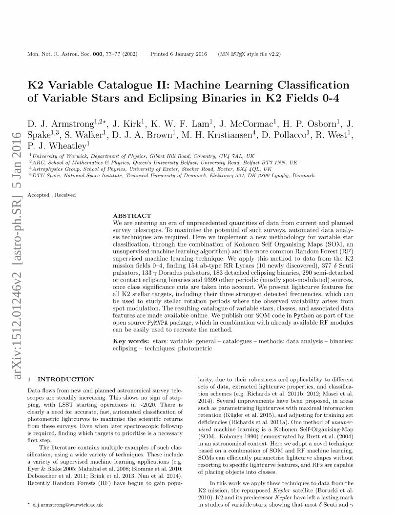
3.3 Training the SOM
There are variations in the literature on how precisely totrain the SOM. Here we run through the procedure followedfor this work. The input parameters are the initial learningrate, α0, which influences the rate at which pixels in theKohonen layer are adjusted, and the initial learning radius,σ0, which affects the size of groups. Initially each pixel israndomised so that each of its 64 elements lies between 0and 1, as our phase curves have been scaled to this range.For each of a series of iterations, each input phase curve iscompared to the Kohonen layer. The best matching pixelin the layer is found, via minimising the difference betweenthe pixel elements and the phase curve. Each element in eachpixel in the layer is then updated according to the expression
mxy,k,new = αe−d2xy2σ2 (sk −mxy,k,old) (2)
where mxy,k is the value m of the pixel at coordinates x,yand element k in the phase curve, dxy is the euclidean dis-tance of that pixel from the best matching pixel in the layer,and sk is the kth element of the considered input phasecurve. This expression is specific to 2-dimensional SOMs,but can be easily adapted for 1-dimension by setting thesize of the second dimension to be 1. Note that distancesare continued across the Kohonen layer boundaries, i.e. theyare periodic. Once this has been performed for each phasecurve, α and σ are updated according to
σ = σ0e
(−i∗log(r)niter
)(3)
α = α0
(1 − i
niter
)(4)
where i is the current iteration, and r is the size of the largestdimension of the Kohonen layer. This is then repeated forniter iterations.
It is possible to use different functional forms for theevolution of α and σ; typically a linear or exponential de-cay is used. Brett et al. (2004) found that the performanceof the SOM was largely unimpeded by the choice of formor initial value, as long as the learning rate does not droptoo quickly. We find satisfactory results for the expressionsabove and values of α0 = 0.1 and σ0 = r, as can be seen inthe below example. The code used in this study was initiallyadapted from the SOM module of the open source PyMVPA
package2(Hanke et al. 2009), and has now been contributedas an update to that package by the authors. As such anyreaders wishing to use this code should look to the given ref-erence. Note that the functional form of Equations 3 and 4
2 http://www.pymvpa.org
are slightly different in the online version of the code, to pre-serve compatibility with older versions of the module. Theformulae described here are the ones used in this work.
As an example we train a SOM on the K2 data fromcampaigns 0-2, as well as Kepler data used for training theclassifier (see Section 3.6 for a full description of the dataset). We use a 40x40 Kohonen Layer. K2 data was only usedif the range of variation in the phase curve before normal-isation was greater than 1.5 times the overall mean of thestandard deviations of points falling in each phase bin (seeprevious Section). This cut was imposed to avoid essentiallyflat lightcurves from impacting the SOM, removing ∼40%of the K2 lightcurves. The majority of these were classifiedas ’Noise’ or ’AP’ in Armstrong et al. (2015), showing thatwe are not removing many periodically varying sources. Wenote that the SOM is robust enough to work without thiscut, and it is imposed only to increase the purity of thetraining set.
We take the known Kepler variables, along with ‘OTH-PER’ other periodic and quasi-periodic objects from K2,and plot them on the resulting SOM in Figure 2. Cleargroups can be seen, with eclipsing binary types well dif-ferentiated but bordering each other, as would be expected.RR Lyraes are very well grouped, and δ Scuti variables clus-ter but more weakly. Example templates from the Kohonenlayer are shown in Figure 3, representing the major clus-ters seen. Note that the size of a group is determined bya number of factors, including the number of input objectsmatching it, and the extent of small variations within thegroup. As there are many more sinusoidal variables thaneclipsing binaries or RR Lyraes, the δ Scuti, γ Doradus and‘OTHPER’ groups fill most of the map. Different regionswithin these groups show for example slight skews from apure sinusoid, and may represent interesting intra-class dif-ferences. δ Scutis lying near the eclipsing binary groups havelikely been mapped using double their true period, and solook similar to a contact binary star. They may also havebeen previously misclassified. It is also interesting to seethat δ Scutis and ‘OTHPER’ objects overlap, as would beexpected given that their phase curve shapes are not par-ticularly distinctive to their respective classes. ‘OTHPER’objects also overlap with the RR Lyrae cluster, and likelymark out newly discovered RR Lyrae stars.
The SOM used for final classification is the same asthat described above, but using only one dimension of 1600pixels. This produces the same clustering results, but is lessuseful for visualisation. We use only one dimension so thatthe other part of our classifier (the RF) can more easily makeuse of the information contained within the SOM.
3.4 Data Features
For the classification of variables into classes, we use a num-ber of specific features of each lightcurve. This is commonpractice in general classification problems (e.g. Richardset al. 2011b). However, there is a subjective element to se-lecting features, and it can be desirable to minimise this ifpossible (see e.g. Kugler et al. 2015). We do so through theuse of the SOM. This encodes the shape of the phase curveinto one parameter (the location of the closest pixel in theSOM to the lightcurve in question), rather than a series of
c© 2002 RAS, MNRAS 000, ??–??

6 Armstrong et. al.
0 5 10 15 20 25 30 35 40SOM X Pixel
0
5
10
15
20
25
30
35
40
SO
M Y
Pix
el
Figure 2. Known variables placed onto a SOM. Random jit-ter within each pixel has been added for clarity. Green triangles
= ’EA’ (detached eclipsing binaries), red crosses = ’EB’ (semi-
detached and contact eclipsing binaries), pink stars = ’RRab’(ab-type fundamental mode RR Lyraes), blue circles = ’DSCUT’
(δ Scuti variables), black dots = ’GDOR’ (γ Dor variables) andyellow pluses = ‘OTHPER’ (other periodic and quasi-periodic ob-
jects). See Section 3.5 for more detail on these variability classes.
0.2
0.4
0.6
0.8
1.0
0.0 0.2 0.4 0.6 0.8 1.00.0
0.2
0.4
0.6
0.8
1.0
0.2 0.4 0.6 0.8 1.0
Phase
Norm
alis
ed A
mplit
ude
Figure 3. Template phase curves from the Kohonen layer of theSOM in Figure 2. Clockwise from top left, templates are for pixel
[13,34] (EA), [6,32] (EB), [37,35] (RRab) and [25,19] (DSCUT).See Section 3.5 for a description of the classes. Note that tem-plates do not have to span the range 0-1, even if the input phasecurves do. Note also that all these templates were found from
initially random pixels without any human guidance or input.
features, none of which may capture the desired shape prop-erties.
There are however other features which are useful andwhich are uninformed by the SOM. A key example is thedominant (most significant) period of the lightcurve. Othersignificant frequencies can also be used, and in some casesmany more have been studied. We only use the three mostsignificant periods here.
The full range of features used is described in Table2. These features are incorporated largely to separate outlightcurves which show purely noise, something which is gen-
erally uninformed by the SOM, as well as those without oneparticularly dominant frequency. We take the potentiallycontroversial step of adjusting some of the noise related fea-tures between the Kepler and K2 datasets, due to the dif-fering noise properties between each set. This is unavoidablehere, as the scatter and increased noise in K2 causes catas-trophic errors in the classifier if Kepler lightcurves are usedas they come. In this case the general result is that the vastmajority of K2 objects are classified as Noise. This prob-lem is solved by multiplying the marked features in Table 2by a factor to align their median values with those of K2.These features are those driven primarily by dataset noise,rather than those associated with periodicity (noise-relatedperiodicity is assumed to have been removed by the pro-cedure in Section 3.2). As the Kepler data used all comesfrom known variable stars, the median of the features is notstrictly comparable to K2, where the data comes from thewhole target list. As such we set the multiplication factorso that the median of the non-eclipsing binary Kepler datafeatures is increased to equal the median of the ‘OTHPER’K2 data features. Eclipsing binaries are left alone, as theirfeatures are in our case dominated by the binary eclipses.
A similar problem arises when studying the PDClightcurves. These have different characteristics to the War-wick lightcurves. Assuming that the intrinsic distribution ofstellar variability should be the same across fields, this differ-ence is due to the differing detrending methods. We adjustfor it in the same way and to the same features as above,marked in Table 2. As we do not have prior classificationsfor fields 3–4, the factor is applied to the whole dataset, andset so as to match the medians of these features between thePDC campaigns 3 and 4 and the Warwick campaigns 0–2.Each PDC campaign is adjusted separately.
It would be desirable to use colour information as afeature to aid classification of variability types connectedto specific stellar spectral types. However, colours are notuniformly available for the K2 sample, although some canbe found through a cross-match with the TESS input catalog(Stassun et al. 2014). As such we do not use them, as doingso would mean large fractions of the K2 targets would needto be disregarded. This has consequences for the variabilityclasses we use, see Section 3.5.
3.5 Classification Scheme
An important decision is in which variability classes to use.We experimented with classifying RR Lyrae (subtype ab),δ Scuti, eclipsing binary (split into detached, subtype EA,and semi-detached or contact, subtype EB), γ Dor, and so-called ROT variables, a class applying to likely rotationallymodulated lightcurves seen in Bradley et al. (2015). We alsoattempted to split the γ Dor class into symmetric, asymmet-ric, and ’MULT’ classes, as defined in Balona et al. (2011).This approach had varied success; RR Lyrae ab, δ Scuti,γ Dor and eclipsing binary classes performed well, but wefound that the γ Dor subtypes were not well constrained byour available features. This may be because we lack suffi-cient training objects to reliably map the range of featuresoffered by these subtypes. This problem could be navigablewhen an increased sample of objects is available through K2,and we plan to address this in later work.
Similarly, we found that the ’ROT’ class was not very
c© 2002 RAS, MNRAS 000, ??–??

K2VarCat II: Machine Learning Classification 7
Table 2. Data Features
Feature Name Description
period Most significant period (Section 3.2)amplitude Max - min of phase curve
period 2 Second detected period (Section 3.2)
period 3 Third detected period (Section 3.2)ampratio 21 period 2 to period amplitude ratio
ampratio 31 period 3 to period amplitude ratio
SOM index Index of closest pixel in 1D SOMSOM distance Euclidean distance to closest pixel
in 1D SOM
p2p 98perc a 98th percentile of point to point scatterin lightcurve
p2p mean a Mean of point to point scatter in lightcurvephase p2p max Maximum point to point scatter in binned
phase curve
phase p2p mean Mean of point to point scatter in binnedphase curve
std ov err a Whole lightcurve standard deviation over
mean point error
a adjusted between datasets, see text.
coherent - the classifier struggled to identify regions in pa-rameter space corresponding to these variables. This likelyarises due to the tendency of this class to have an indis-tinct cluster of low frequency peaks rather than one clearsignal (Bradley et al. 2015). Rather than use the ROT classby itself, we make use of the previous version of this cata-logue, which contained a ‘QP’ quasiperiodic variable class.This class contains a number of variable types, but is charac-terised by periodic variability that is not strictly sinusoidal,and changes in amplitude and/or period. We use this as avariable classification, to catch interesting variables of as-trophysical origin which are not one of the five other classes(RR Lyrae ab, EA, EB, δ Scuti, γ Dor). It is likely dominatedby spot-modulated stars, but also contains other variablessuch as Cepheids. We rename this class to ‘OTHPER’ for‘other periodic’ to avoid confusion, as variables which arestrictly periodic but not in another class can be classified bythis group.
We considered including other variable classes, such asCepheids, the other RR Lyrae subtypes (first-overtone ormultimode RR Lyraes), and Mira variables. We could notfind sufficient training set objects in any of these classes (lessthan 20 in each case). While it is possible to attempt classi-fication with small training sets, rather than present a weakor unreliable classification for these classes we prefer to waitfor more K2 data. As more fields are observed, more train-ing set objects will become available. We intend to includemore classes in future versions of this catalogue.
Finally, we include ’Noise’, non-variable lightcurves, asa class label. This leave 7 classes, DSCUT (δ Scuti), GDOR(γ Doradus), EA (detached eclipsing binaries), EB (semi-detached and contact eclipsing binaries), OTHPER (otherperiodic and quasi-periodic variables), RRab (RR Lyrae abtype) and Noise. It is important to note that as we do nothave colour information, there will be degeneracy in the DS-CUT class between true δ Scutis and β Ceph variables, asin Debosscher et al. (2011). This is also true for slowly pul-sating B stars, which are degenerate with γ Dor variables.
3.6 Training Set
Although the SOM described is unsupervised and so requiresno training set, the RF classifier we use for final classificationdoes. An ideal training set would consist of a set of knownvariable stars from the K2 mission, to which we can fit theclassifier. Some previous classification work on K2 has beendone (for B stars (Balona et al. 2015), for eclipsing binaries(LaCourse et al. 2015), and in the previous version of thiscatalogue). These sources however suffer from either smallnumbers, only being applicable to a few variable types, or inthe Armstrong et al. (2015) case using variability classes de-rived from the lightcurves rather than externally recognisedtypes. We cross matched the observed K2 targets in fields0–3 (4 was not available at that time) with catalogues ofknown variable stars, including those from AAVSO3, GCVS(Samus et al. 2009) and ASAS (Richards et al. 2012). Thisled to a small number of targets (a few tens of each class atbest), not enough for a full training set. As such, we turnedto the original Kepler mission. Much classification work hasbeen done on the Kepler lightcurves. The data has differingnoise properties to K2 data, but the same cadence, instru-ment, and if only one 90 day quarter of data is used a similarbaseline to a K2 campaign.
Although multiple works are available offering classifiedvariable stars in Kepler, we limit ourselves to a small num-ber of relatively large scale catalogues, in order to maintainhomogeneity among classification methods and simplify theprocess. We began by taking the EA, EB, DSCUT classesfrom Bradley et al. (2015) We also took ROT, SPOTM andSPOTV, low frequency variables likely due to rotationalmodulation, reclassifying these objects as OTHPER. Wesupplemented the DSCUT set with those from Uytterho-even et al. (2011). The bulk of our eclipsing binary trainingset come from the Kepler Eclipsing Binary Catalogue (Prsaet al. 2011; Slawson et al. 2011). We removed all heartbeatbinaries (Thompson et al. 2012) and those where the pri-mary eclipse depth was less than 1%. A threshold of 1% wasimplemented in order to avoid shallow, likely blended binaryeclipses from being included in the training set and henceincrease training set purity. This also avoids the problemof noisy lightcurves with instrumental systematics of ordera percent being misclassified as eclipsing binaries. Binarieswere then classified as EA or EB based on a morphologythreshold of 0.5 (see Matijevic et al. (2012) for a discussionof morphology in this context). For RR Lyrae stars we usethe list in Nemec et al. (2013). Fundamental mode subtypeab stars were labelled RRab, and the first-overtone subtypec stars classified as OTHPER. To increase this relativelysmall RR Lyrae sample we used the results from the K2AAVSO cross-match, taking fundamental mode RR Lyraesand adding them to the RRab training set. The B-star cat-alogue of Balona et al. (2015) was also used, with the SPBclass reclassified as GDOR (given the degeneracy betweenGDOR and SPB present without temperature information)and the ROT class being reclassified as OTHPER.
For the OTHPER and Noise classes, we also use ourprevious catalogue. This contained 5445 OTHPER (QP inthe original catalogue) and 29228 Noise objects in fields 0–2, with labels assigned by human eyeballing. To avoid hav-
3 www.aavso.org
c© 2002 RAS, MNRAS 000, ??–??

8 Armstrong et. al.
Table 3. Training Set
Class N objects
RRab 91DSCUT 278
GDOR 233EA 694
EB 759
OTHPER 1992Noise 976
ing an excessive disparity between training set classes, wedownsample this set to 1000 of each class, selected ran-domly, which are then added on to the Kepler OTHPERset above. This also makes the results on fields 0–2 moreindependent, as we can compare previously classified OTH-PERs (the majority of which are now not in the trainingsample) with newly found ones. To reduce the impact of po-tential mistakes in the previous catalogue, we removed thesmall number of objects in the OTHPER training set whichwere in an initial run of this classifier reclassified as anotherclass. Objects with a probability of being in the RRab classof greater than 0.2 were also removed, as the probabilitiesfor the RRab class are not well calibrated (see Section 3.8).These cuts caught ∼50 objects misclassified as OTHPERand ∼30 objects misclassified as Noise out of the 1000 eachinitially selected.
The final classes and number of objects in each trainingset are shown in Table 3.
3.7 Random Forest Implementation
We use the implementation of RFs in the scikit-learn
Python module4. There are several input parameters for anRF classifier. The key ones are the number of estimators, themaximum features considered at each branch in the compo-nent decision trees, and the minimum number of samplesrequired to split a node on the tree, which controls howfar each tree is extended. In a typical case, increasing thenumber of estimators always leads to improvement in per-formance but with decreasing returns and increasing com-putation time. The theoretical optimum maximum featuresfor a classification problem is the square root of the totalnumber of features, in our case 3. We optimise the parame-ters using the ’out-of-bag’ score of the RF. When training,the classifier uses a random subset of the total data samplegiven to it for each tree, to reduce the chance of bias. Theleft out data is then used to test the performance of the tree– its known class is compared to the predicted class, givinga performance metric between 0 (for absolute failure) and 1(for perfect classification). Maximising this metric allows usto optimise the parameters. We find the best results for 300estimators, a maximum of 3 features, and 5 samples to splita node. These parameters are used for classification. Addi-tionally we apply weights to the training set, so that eachclass is inversely weighted according to its frequency in thetraining set (input option class weight=‘auto’). This makessure that classes with more members (such as OTHPER and
4 http://scikit-learn.org/stable/
DSC
UT
EA EB
GD
OR
Nois
e
OTH
PER
RR
ab
Predicted Class
DSCUT
EA
EB
GDOR
Noise
OTHPER
RRab
Tru
e C
lass
0.5935
0.0029
0.0026
0.2017
0.0532
0.1165
0.9135
0.0277
0.0086
0.0184
0.0045
0.0432
0.946
0.0102
0.0126
0.011
0.1115
0.0043
0.1631
0.0982
0.1291
0.044
0.0971
0.0187
0.0145
0.2403
0.5307
0.2034
0.022
0.1978
0.0159
0.0092
0.3691
0.2822
0.5138
0.0879
0.0014
0.0172
0.0072
0.0201
0.8352
Figure 4. Confusion matrix for a RF considering only SOM
map location, generated using leave-one-out cross validation. Textshows the percentage of each sample which was classified into the
relevant box. Correct classification lies on the diagonal.
Noise) do not drown out other classes, and in effect imposesa uniform prior on the class probabilities.
There are several random elements in our method.These are the selection of the OTHPER and Noise trainingsets, as well as certain elements of the RF. Random subsetsof training objects and features are selected for each decisiontree as part of the RF method, to avoid bias. To minimiseany effects of this randomness (especially the OTHPER andNoise selection), we train 50 classifiers with the above pa-rameters and repeat the selection for each, applying eachclassifier to the K2 dataset. The average class probabilityacross the classifiers gives the final result.
To explore the power of the SOM method, we trial theRF on only the SOM map location (SOM index). The clas-sifier is cross-validated by taking one training set memberand training the classifier on the remaining members (so-called leave-one-out cross validation). The left out object isthen tested on the classifier, and the process repeated foreach member. The performance of the classifier is best de-scribed by a ‘confusion matrix’, shown in Figure 4. Thisshows what proportion of training members in each classwere assigned to which other classes. In the ideal case eachobject is predicted correctly. Here we can see clearly whichclasses are well-informed by the SOM. RRab, EA, and EBclasses are strongly recovered, as expected from their stronglocalisation in Figure 2. The DSCUT class is also recoveredalthough less so. On the other side, OTHPER and Noiseclasses are found more weakly, and GDOR barely at all,due to the often multiple pulsation frequencies in this classcombining to produce no distinctive phase curve shape. Thisdemonstrates the power of the SOM alone to classify certainclasses of variable stars.
Moving on to the full classification scheme, we test theRF in a similar manner. All 7 classes are used, and the classi-
c© 2002 RAS, MNRAS 000, ??–??

K2VarCat II: Machine Learning Classification 9D
SC
UT
EA EB
GD
OR
Nois
e
OTH
PER
RR
ab
Predicted Class
DSCUT
EA
EB
GDOR
Noise
OTHPER
RRab
Tru
e C
lass
0.9964
0.0026
0.0043
0.002
0.9568
0.0277
0.0015
0.0331
0.9671
0.0045
0.7597
0.0136
0.9039
0.0894
0.0036
0.0101
0.0026
0.2318
0.0961
0.8885
0.033
0.0043
0.0005
0.967
Figure 5. Confusion matrix for a RF considering all featuresand classes, generated using leave-one-out cross validation. Text
shows the percentage of each sample which was classified into therelevant box. Correct classification lies on the diagonal.
fier cross-validated as before. The resulting confusion matrixis shown in Figure 5. It highlights some interesting cases.Firstly, the classifier works well, with an overall success rateof 92.0%. There is some porosity between the two eclips-ing binary classes, with objects of one class being placedinto the other. As there is no rigid boundary in lightcurveshape between them, this is to be expected. Similarly thereis some spread between OTHPER and Noise. This is notdesirable, but the numbers involved are low, and representobjects with either variability only just emerging above thenoise or objects with unusual noise properties. The biggestmisclassification occurs between the GDOR and OTHPERclasses. This arises due to the less distinct nature of theOTHPER class - it acts as a ‘catch-all’ class to find any pe-riodic or quasi-periodic variables which do not fit the otherclasses. GDOR objects can in some circumstances presentsimilar lightcurve features to for example fast rotating stars,leading to some confusion between the classes.
One advantage of RF classifiers is the ability to esti-mate feature importance. The classifier naturally measureswhich features have more descriptive power, through for ex-ample how often those features are used in the decision trees,or through the reduction in performance that would be ob-served is a feature was replaced by a randomly sampled dis-tribution. This allows for model refinement, and is of greatuse in developing a classifier. We plot the importance of ourfeatures in Figure 6. These are found through training theclassifier 100 times, and extracting the mean and standarddeviation of the feature importances for each classifier.
0.00 0.05 0.10 0.15 0.20Feature Importance
ampratio_21
SOM_distance
ampratio_31
phase_p2p_mean
period_3
period_2
phase_p2p_max
p2p_mean
std_ov_err
p2p_98perc
amplitude
SOM_index
period
Figure 6. Relative importance of features to the RF. Values anderrors arise from the mean and standard deviation of the feature
importances extracted from 100 trained classifiers.
3.8 Class posterior probability calibration
The RF classifier automatically generates class probabili-ties (through the proportion of estimators classifying an ob-ject into each class). These probabilities are not necessarilyaccurate. Although it is true that higher class probabilitymeans more likelihood of an object being in that class, theprobabilities can need calibrating to ensure that they aretrue posterior probabilities. This is where, if a set of objectshave probability p that they are in a certain class, the sameproportion of them actually are of that class.
Initially we test the calibration of our ‘raw’ class prob-abilities. Figure 7 shows the class probabilities found fromthe cross validated training set data created as describedin Section 3.7. This allows the predicted class probabilitiesfor each training set object to be compared to their knownclasses. They are clearly not true posterior probabilities, es-pecially for the RRab class, where essentially every objectwith class probability > 0.5 is a true class member. For theother classes the given probabilities are closer, but still showsome departure from the ideal case.
One common way of testing classifier performance inthis way is the Brier score (Brier 1950). Our raw probabil-ities have a Brier score of 0.1336. We attempted a numberof methods of calibrating them (and so reducing this score).The most usual methods are sigmoid and isotonic regression,which fit certain functions to the calibration curve to trans-form the probabilities. Similarly to Richards et al. (2012),we find that these methods are not effective in our case. Weattempted the method of Bostrom (2008) to transform theinitial class probabilities, but also found the results to beunsatisfactory. Rather than present an incomplete calibra-tion, we give the class probabilities as they are. Users shouldbe aware of this, and avoid interpreting class probabilitiesas true posterior probabilities.
As the training set will not be representative of the trueK2 distribution, biases may exist. As the priors are not wellknown, and the distribution of training sources by no meansmatches the underlying distribution of variables in K2, trueposterior probabilities are impossible to create. Hence thegiven class probabilities, even if calibrated, would only beposterior probabilities under the assumption that each classhas a uniform probability of arising.
c© 2002 RAS, MNRAS 000, ??–??

10 Armstrong et. al.
0.0 0.2 0.4 0.6 0.8 1.0Predicted Probabilities
0.0
0.2
0.4
0.6
0.8
1.0
Tru
e P
robabili
ties
Figure 7. Overall classifier predicted probability against trueprobability for the RRab class (crosses) and the average of all
other classes (dots). The straight black dashed line represents the
ideal case.
4 CATALOGUE
4.1 Overview
The full catalogue for K2 fields 0–4 inclusive is given in Ta-ble 4. This Table contains classifications using the Warwicklightcurves, as described in Section 2.2. The features usedto classify these objects are given in Table 5. We also runthe classifier on the PDC lightcurves produced by the K2mission team. These were only available for campaigns 3–4.The resulting classifications are given in Table 6, and theirassociated features in Table 7.
c© 2002 RAS, MNRAS 000, ??–??

K2V
arCat
II:M
achine
Learn
ing
Classifi
cation11
Table 4. Catalogue table for our Warwick detrended lightcurves. Fields 0–4 are included. Only an extract is shown here for guidance in form. The full table is available online.
K2 ID Campaign Class Class Probabilities Anomaly
DSCUT EA EB GDOR Noise OTHPER RRab
202059070 0 Noise 0.004195 0.120507 0.016615 0.005925 0.604636 0.246088 0.002034 0.023891
. . . . . . . . . . .
Table 5. Data features for our Warwick detrended lightcurves. Fields 0–4 are included. Only an extract is shown here for guidance in form. The full table is available online.
K2 ID Campaign SOM index period period 2 period 3 SOM distance phase p2p mean phase p2p max amplitude ampratio 21 ampratio 31
d d d rel. flux rel. flux rel. flux
202059070 0 1544 4.764370 1.241680 0.174448 1.180831 0.003801 0.487419 0.042283 0.629987 0.548721
. . . . . . . . . . . .
p2p mean p2p 98perc std ov err
rel. flux rel. flux
0.016326 0.047548 1.310764
. . . . . . . . . . . .
Table 6. Catalogue table for PDC detrended lightcurves. Fields 3–4 only. Only an extract is shown here. The full table is available online.
K2 ID Campaign Class Class Probabilities Anomaly
DSCUT EA EB GDOR Noise OTHPER RRab
205889250 3 Noise 0.000067 0.000000 0.000000 0.000030 0.966544 0.033359 0.000000 0.000000
. . . . . . . . . . .
Table 7. Data features for PDC detrended lightcurves. Fields 3–4 only. Only an extract is shown here. The full table is available online.
K2 ID Campaign SOM index period period 2 period 3 SOM distance phase p2p mean phase p2p max amplitude ampratio 21 ampratio 31d d d rel. flux rel. flux rel. flux
205889250 3 0630 19.754572 12.803889 2.281881 1.179035 0.003795 0.421976 0.008715 0.741302 0.592596. . . . . . . . . . . .
p2p mean p2p 98perc std ov errrel. flux rel. flux
0.005249 0.017133 1.371857. . . . . . . . . . . .
c©2002
RA
S,
MN
RA
S000
,??–??

12 Armstrong et. al.
Table 8. Total objects in each class.
Class Total Prob > 0.5 Prob > 0.7 Prob > 0.9
RRab 248 154 72 25DSCUT 750 562 377 166
GDOR 451 264 133 37EA 607 308 183 99
EB 463 392 290 186
OTHPER 22428 18698 9399 3547Noise 43963 38609 21210 6018
The total number of objects found in each class is givenin Table 8, at various probability cuts. Note that for RRabclass objects in particular, most objects with class probabil-ity > 0.5 are real classifications. In the other cases the prob-ability calibration is better, but these probabilities shouldstill not be interpreted as posterior probabilities.
We find that the classifier works well on all fields. TheRRab class performs well throughout, due to the distinctiveshape of their phasecurves. These are well characterised bythe SOM. There are however some distinct features uniqueto fields 3 and 4. The EA class has a tendency to pick upnoise dominated lightcurves in these fields, primarily be-cause their point to point scatter is much higher than infields 0–2. In these cases the class probability, although high-est for EA, is still relatively low however. Similarly for DS-CUT objects, there are a higher proportion of objects inthese fields with many anomalous points, possibly due toflaring or instrumental noise. These points can cause biasesin the phase curve, resulting in an artificial sinusoid, whichwhen combined with a short period results in a DSCUT clas-sification. Again these noise objects have a lower probabilitythan real DSCUT lightcurves. One final interesting propertyis the split between OTHPER and Noise lightcurves. Thisis good for fields 0–2. In fields 3 and 4, while OTHPERlightcurves are recognised, several Noise lightcurves can beclassified as OTHPER. Probability cuts remove the worstof these, but there is no way to distinguish between quasi-periodic instrumental noise and astrophysical variability inthis scheme. These issues all lead to the conclusion that theclassifier has more trouble with fields 3–4, due to a patternof increased noise. We expect this issue to improve as K2detrending methods become more robust.
4.2 Detrending method comparison
Table 9 shows the numbers of variable stars found using eachdataset. At first glance the numbers in Table 9 seem to im-ply significant differences between detrending methods. Thediscrepancy in RRab numbers is largely a result of differingprobability calibration - the same stars are found in bothdatasets, but those in the Warwick set given lower proba-bilities (although still higher than all other classes). Othermajor discrepancies are in the GDOR and EA classes. ForGDOR, we find that the PDC set gives better results. Sev-eral GDOR lightcurves are misclassified in the Warwick setdue to poor detrending masking the true variability. In somecases the PDC GDOR classification is inaccurate, but thisis rare for the class probability > 0.7 objects. For the EAobjects, the reverse is true. Several PDC lightcurves are mis-classified as EA due to a higher number of lightcurves in the
PDC set with very significant remnant outliers. These leadto a high point-to-point scatter, which is interpreted by theclassifier as an eclipse. Here the Warwick set is more reliable.The largest absolute difference in the variable classes is inthe OTHPER objects, where ∼1000 lightcurves extra passthe high probability cut for the PDC set. This is partly aresult of a similar effect as for the RRab objects, where sim-ilarly classified objects are given lower probabilities in theWarwick set. However, there are also several objects foundin the PDC set which are missed in the Warwick set, due toincreased noise levels. The converse is also true, with somelightcurves found in the Warwick set but missed by the PDC.Overall, the two detrending methods perform comparablywell, and can be used to reinforce each other when studyingvariable classes.
4.3 Anomaly detection
Due to the limited classification scheme used, it is inevitablethat some objects will not fit any of the given classes (Pro-topapas et al. 2006). Due to the inclusion of Noise and OTH-PER as classes, this is not a large problem as each classis quite broad. However it is worth noting any particularanomalies. One way of doing this is already intrinsic to theSOM – the Euclidean distance of a phase curve to its nearestmatching pixel template. However this metric only works forperiodic sources, and can flag high for noisy sources. We per-form a check for anomalies following the method of Richardset al. (2012). This works by extracting the proximity mea-sure, ρij between each tested object i and each object j inthe training set. The proximity measure is the proportion oftrees in the classifier for which each object ends at the samefinal classification. It is close to unity for similar objects,and close to zero for dissimilar ones. From the proximitythe discrepancy d is calculated, via
dij =1 − ρijρij
(5)
The anomaly score is then given by the second smallestdiscrepancy of an object to the training set. High anomalyscores represent objects which are not well explained by anyobject in the training set, and are hence outliers.
We find that in this case, the highest few percentilesof anomalous objects are a mixture of noise-dominatedlightcurves, unusual eclipsing binaries and variability whichdoes not fit into the used classification scheme. We leave afull analysis of these unusual lightcurves to future work.
4.4 Eclipsing Binaries
Encouragingly we identify 139 (96 at class probability > 0.7)of the 165 EPIC, non-M35 eclipsing binaries identified byLaCourse et al. (2015) in field 0 as either ’EA’ or ’EB’ type,despite automating the process and not focusing on exclu-sively eclipsing binaries. The majority of the remainder areidentified as ’OTHPER’ or ’DSCUT’, and are discussed be-low. We further identify an additional 61 EPIC, non-M35objects in field 0 as ’EA’ or ’EB’ at class probability > 0.7,although as our identification is automated rather than vi-sual some of these may be misidentified by the classifier.Many more eclipsing binaries are found in the other fields.
c© 2002 RAS, MNRAS 000, ??–??

K2VarCat II: Machine Learning Classification 13
Table 9. Total objects in each class in fields 3–4, split by detrending method (W=Warwick, PDC=K2 Team released lightcurves).
Class Total W Total PDC Prob > 0.5 W Prob > 0.5 PDC Prob > 0.7 W Prob > 0.7 PDC
RRab 141 152 95 115 48 83
DSCUT 280 266 180 201 116 148GDOR 198 382 122 238 61 101
EA 255 413 97 223 54 102
EB 168 150 140 131 106 105OTHPER 11402 9102 8709 8034 3522 4565
Noise 17143 19126 13012 17919 3625 11566
Table 10. EPIC IDs for 29 visually identified eclipsing binariesclassified as ‘OTHPER’ by our classifier, from fields 0–4.
201158453 201173390 201569483 201584594201638314 202072962 202137580 203371239
203476597 203637922 204043888 204193529
204328391 204411840 205510143 205919993205985357 205990339 206047297 206060972
206066862 206226010 206311743 206500801210350446 210501149 210766835 210945342
211093684 211135350
The previously labelled, but not identified by our clas-sifier, eclipsing binaries fall into three main groups. The firstshow near-sinusoidal short period lightcurves, and are gen-erally identified as ’DSCUT’. In these cases it is difficult toreliably assign a class with the information available. Theseobjects may be actual δ Scuti stars, or contact eclipsingbinaries. The other and largest group, with 14 members,are identified as ’OTHPER’, and show pulsations or spot-modulation in addition to the known eclipses. We note thatthe classifier will assign a class based largely on the domi-nant period and phasecurve at this period, hence performsas expected in these cases. Pulsating stars in eclipsing bi-naries are useful objects, and so while a detailed study ofthese objects is beyond the scope of this paper we provide alist of such objects in Table 10. These are eclipsing binariesidentified by a visual check of the lightcurves performed our-selves (as the LaCourse et al. (2015) catalogue only coveredfield 0), which are classified as ‘OTHPER’ by our classifier.Some may be blended signals, and hence the pulsator orspot-modulated star may not be a member of the eclipsingbinary system.
4.5 δ Scuti Stars
We have a sample of 377 δ Scuti candidates, using a classprobability cut of 0.7. The majority of these candidateswere previously unknown. It is interesting to study their fre-quency and amplitude distribution. Note that here we useamplitude defined as in the max-min of the binned phasecurve, and semi-amplitude as half this value. The distribu-tion of amplitudes for the 377 δ Scuti candidates is shownin Figure 8. We see a number of HADS (high amplitude δScutis). Using an amplitude threshold of 104 ppm as usedby Bradley et al. (2015), 104 of our candidates are HADS.Included in this sample are 11 candidates with an ampli-tude greater than 105 ppm. The period distribution of thewhole sample is shown in Figure 9, and covers the expected
2.0 2.5 3.0 3.5 4.0 4.5 5.0 5.5 6.0Log10(amplitude/ppm)
0
10
20
30
40
50
60
70
N C
andid
ate
s
Figure 8. The distribution of phase curve amplitude for DSCUT
classified objects. Several high amplitude candidates are visible.
0.05 0.10 0.15 0.20 0.25Period (d)
0
10
20
30
40
50
60
70
80
90
N C
andid
ate
s
Figure 9. The distribution of pulsation periods for DSCUT clas-sified objects. The cutoff at the low period end is imposed by ourNyquist sampling frequency.
range for δ Scuti variables, limited by our Nyquist samplingfrequency.
As has been mentioned, the DSCUT classified objectsare degenerate with β Ceph variables due to the lack ofcolour information available. There is a catalogue of esti-mated K2 temperatures available for some objects (Stassun
c© 2002 RAS, MNRAS 000, ??–??

14 Armstrong et. al.
3.0 3.5 4.0 4.5Log10(amplitude/ppm)
0
5
10
15
20
N C
andid
ate
s
Figure 10. The distribution of phase curve amplitude for GDORclassified objects.
0.0 0.5 1.0 1.5 2.0 2.5 3.0Period (d)
0
5
10
15
20
N C
andid
ate
s
Figure 11. The distribution of pulsation periods for GDOR clas-
sified objects.
et al. 2014) which could be used to make probable distinc-tions if necessary.
4.6 γ Doradus Stars
We have a sample of 133 γ Doradus candidates, using a classprobability cut of 0.7. We plot the amplitude and period dis-tributions in Figures 10 and 11, following the same definitionof amplitude as for the δ Scuti sample. Note that this am-plitude is only for the dominant period phase curve, andso does not include the other significant frequencies oftenpresent in γ Doradus lightcurves. The period distributioncovers the expected range for γ Doradus variables. Due tothe lack of colour information available, γ Doradus objectsare degenerate with slowly pulsating B stars.
4.7 RR Lyrae ab-type Stars
As the RRab class has less well calibrated probability (al-most all candidates with Prob(RRab) greater than 0.5 seem
5.0 5.5 6.0 6.5 7.0 7.5Log10(amplitude/ppm)
0
10
20
30
40
50
60
N C
andid
ate
s
Figure 12. The distribution of phase curve amplitude for RRabclassified objects.
to be real) we use an adjusted class probability thresholdof 0.5 to study this class. This leaves 154 candidates. Theiramplitude distribution is shown in Figure 12, and peaks atsignificantly higher amplitude than that of the DSCUT andGDOR candidates as would be expected. Most of these can-didates are previously known; we find that 129 of them arein K2 proposals focused on RR Lyrae stars. These proposalscontain both known and candidate RR Lyraes; in the candi-date cases our classification provides some support for themtruly being RR Lyrae variables. Assuming these proposalswere comprehensive (reasonable, given the multiple teamsinvolved), this leaves 25 candidates as potential new discov-eries by this catalogue. However, as these objects are thosenot in the proposals, there is a selection effect in favour ofmisclassified non-RR Lyrae objects. We performed a visualexamination of each of these 25 lightcurves, which resultedin 8 of the 25 being confirmed as real RR Lyrae candidates(the others being either misclassified outbursting stars orparticularly high amplitude noise). An additional 3 candi-dates were found by using the PDC lightcurve set and check-ing objects in both sets with class probability between 0.4and 0.5, resulting in 10 total new candidates. These objectsmay still be blends of true RR Lyraes, hence the candidatedesignation. We plot the phase folded lightcurves for twonew discoveries and two known RR Lyrae stars in Figure13. Some amplitude modulation can be seen, due to someof these targets exhibiting the Blazhko effect (Blazko 1907).RR Lyraes are immensely useful objects, allowing studies ofthe evolution of stellar populations throughout the Galaxyand in other nearby galaxies. Due to an absolute magnitude-metallicity relation (Sandage 1981) it is possible to use themfor distance estimation.
5 CONCLUSION
We have implemented a novel combined machine learningalgorithm, using both Self Organising Maps and RandomForests to classify variable stars in the K2 data. We considerfields 0–4, and intend to update the catalogue as more fieldsare released. As more data builds up, it may become possible
c© 2002 RAS, MNRAS 000, ??–??

K2VarCat II: Machine Learning Classification 15
0.6
0.8
1.0
1.2
1.4
1.6
1.8
2.0
Rela
tive F
lux
0.0 0.2 0.4 0.6 0.8 1.0Phase
0.6
0.8
1.0
1.2
1.4
Rela
tive F
lux
0.2 0.4 0.6 0.8 1.0Phase
Figure 13. Four phase folded RRAB classified lightcurves. Clock-wise from top-left, the EPIC IDs are 210830646, 206409426,
211069540 and 203692906.
to implement new variability classes, and study the effect ofdifferent detrending methods on the catalogue performance.We obtain a success rate of 92% using out of bag estimateson the training set.
We train the classifier on a set of Kepler and some K2data from fields 0–2. As such it is applied completely inde-pendently to the majority of the K2 data, and the whole offields 3–4. That we obtain good results for fields 3–4 bodeswell for application of the classifier to future data.
Algorithms like this will become an increasingly impor-tant step in processing the data volumes expected from fu-ture astronomical surveys. To maximise scientific return itis critical to select interesting candidates, and do so rapidlyand with minimal input. We hope that this method will con-tribute to the growing body of work attempting to addressthis issue.
ACKNOWLEDGEMENTS
The authors thank the anonymous referee for a helpful re-view of the manuscript. This paper includes data collectedby the Kepler mission. Funding for the Kepler mission is pro-vided by the NASA Science Mission directorate. The datapresented in this paper were obtained from the MikulskiArchive for Space Telescopes (MAST). STScI is operatedby the Association of Universities for Research in Astron-omy, Inc., under NASA contract NAS5-26555. Support forMAST for non-HST data is provided by the NASA Office ofSpace Science via grant NNX13AC07G and by other grantsand contracts. We acknowledge with thanks the variable starobservations from the AAVSO International Database con-tributed by observers worldwide and used in this research.
REFERENCES
Aigrain S., Hodgkin S. T., Irwin M. J., Lewis J. R., RobertsS. J., 2015, Monthly Notices of the Royal AstronomicalSociety, 447, 2880
Armstrong D. J. et al., 2015, Astronomy and Astrophysics,579, A19
Balona L. A., Baran A. S., Daszy ska Daszkiewicz J.,De Cat P., 2015, Monthly Notices of the Royal Astro-nomical Society, 451, 1445
Balona L. A., Dziembowski W. A., 2011, Monthly Noticesof the Royal Astronomical Society, 417, 591
Balona L. A., Guzik J. A., Uytterhoeven K., Smith J. C.,Tenenbaum P., Twicken J. D., 2011, Monthly Notices ofthe Royal Astronomical Society, 415, 3531
Blazko S., 1907, Astronomische Nachrichten, 175, 325Blomme J. et al., 2010, The Astrophysical Journal, 713,L204
Borucki W. J. et al., 2010, Science, 327, 977Bostrom H., 2008, in Proc. 7th International Conf. MachineLearning and Applications. IEEE, pp 121–126
Bradley P. A., Guzik J. A., Miles L. F., UytterhoevenK., Jackiewicz J., Kinemuchi K., 2015, The Astronomi-cal Journal, 149, 68
Breiman L., 2001, Machine Learning, 45, 5Brett D. R., West R. G., Wheatley P. J., 2004, MonthlyNotices of the Royal Astronomical Society, 353, 369
Brier G. W., 1950, Monthly Weather Review, 78, 1Brink H., Richards J. W., Poznanski D., Bloom J. S., RiceJ., Negahban S., Wainwright M., 2013, Monthly Noticesof the Royal Astronomical Society, 435, 1047
Carrasco Kind M., Brunner R. J., 2014, Monthly Noticesof the Royal Astronomical Society, 438, 3409
Debosscher J., Blomme J., Aerts C., De Ridder J., 2011,Astronomy and Astrophysics, 529, A89
Eyer L., Blake C., 2005, Monthly Notices of the Royal As-tronomical Society, 358, 30
Grigahcene A. et al., 2010, The Astrophysical Journal, 713,L192
Hanke M., Halchenko Y. O., Sederberg P. B., Hanson S. J.,Haxby J. V., Pollmann S., 2009, Neuroinformatics, 7, 37
Howell S. B. et al., 2014, Publications of the AstronomicalSociety of the Pacific, 126, 398
Kohonen T., 1990, Proceedings of the IEEE, 78, 1464Kugler S. D., Gianniotis N., Polsterer K. L., 2015, MonthlyNotices of the Royal Astronomical Society, 451, 3385
LaCourse D. M. et al., 2015, Monthly Notices of the RoyalAstronomical Society, 452, 3561
Lomb N. R., 1976, Astrophysics and Space Science, 39, 447Lund M. N., Handberg R., Davies G. R., Chaplin W. J.,Jones C. D., 2015, The Astrophysical Journal, 806, 30
McQuillan A., Aigrain S., Mazeh T., 2013, Monthly Noticesof the Royal Astronomical Society, 432, 1203
McQuillan A., Mazeh T., Aigrain S., 2014, The Astrophys-ical Journal Supplement Series, 211, 24
Mahabal A. et al., 2008, Astronomische Nachrichten, 329,288
Masci F. J., Hoffman D. I., Grillmair C. J., Cutri R. M.,2014, The Astronomical Journal, 148, 21
Matijevic G., Prsa A., Orosz J. A., Welsh W. F., BloemenS., Barclay T., 2012, The Astronomical Journal, 143, 123
Molnar L., Pal A., Plachy E., Ripepi V., Moretti M. I.,Szabo R., Kiss L. L., 2015, eprint arXiv:1508.05587
Nemec J. M., Cohen J. G., Ripepi V., Derekas A., MoskalikP., Sesar B., Chadid M., Bruntt H., 2013, The Astrophys-ical Journal, 773, 181
Nun I., Pichara K., Protopapas P., Kim D.-W., 2014, The
c© 2002 RAS, MNRAS 000, ??–??
16 Armstrong et. al.
Astrophysical Journal, 793, 23Press W. H., Rybicki G. B., 1989, The Astrophysical Jour-nal, 338, 277
Protopapas P., Giammarco J. M., Faccioli L., StrubleM. F., Dave R., Alcock C., 2006, Monthly Notices of theRoyal Astronomical Society, 369, 677
Prsa A. et al., 2011, The Astronomical Journal, 141, 83Richards J. W. et al., 2011a, The Astrophysical Journal,744, 192
Richards J. W. et al., 2011b, The Astrophysical Journal,733, 10
Richards J. W., Starr D. L., Miller A. A., Bloom J. S.,Butler N. R., Brink H., Crellin-Quick A., 2012, The As-trophysical Journal Supplement Series, 203, 32
Samus N. N., Durlevich O. V., Kazarovets E. V., KireevaN. N., Pastukhova E. N., Zharova A. V., 2009, Instituteof Astronomy of Russian Academy of Sciences and Stern-berg State Astronomical Institute of the Moscow StateUniversity
Sandage A., 1981, The Astrophysical Journal, 248, 161Scargle J. D., 1982, The Astrophysical Journal, 263, 835Slawson R. W. et al., 2011, The Astronomical Journal, 142,160
Smith J. C. et al., 2012, Publications of the AstronomicalSociety of the Pacific, 124, 1000
Stassun K. G., Pepper J. A., Paegert M., De Lee N.,Sanchis-Ojeda R., 2014, eprint arXiv:1410.6379
Stumpe M. C. et al., 2012, Publications of the AstronomicalSociety of the Pacific, 124, 985
Thompson S. E. et al., 2012, The Astrophysical Journal,753, 86
Tkachenko A. et al., 2013, Astronomy and Astrophysics,556, A52
Torniainen I. et al., 2008, Astronomy and Astrophysics,482, 483
Torrence C., Compo G. P., 1998, Bulletin of the AmericanMeteorological Society, 79, 61
Uytterhoeven K. et al., 2011, Astronomy and Astrophysics,534, A125
Vanderburg A., Johnson J. A., 2014, Publications of theAstronomical Society of the Pacific, 126, 948
c© 2002 RAS, MNRAS 000, ??–??