Jupiter's Tropospheric Thermal Emission. II. Power Spectrum Analysis and Wave Search

ICARUS 124, 32–44 (1996)ARTICLE NO. 0188

Jupiter’s Tropospheric Thermal Emission

II. Power Spectrum Analysis and Wave Search

JOSEPH HARRINGTON1 AND TIMOTHY E. DOWLING

Department of Earth, Atmospheric, and Planetary Sciences, Room 54-410, Massachusetts Institute of Technology, Cambridge, Massachusetts 02139E-mail: [email protected]

AND

RICHARD L. BARON

Institute for Astronomy, University of Hawaii, Honolulu, Hawaii 96822

Received June 30, 1995; revised June 20, 1996

be identified with periodic features such as vortex chains andthe equatorial plumes. The origin of others is less certain. WeWe study power spectra and search for planetary waves inpresent a table of our best wave candidates. 1996 Academic Press, Inc.images of Jupiter’s cloud opacity. The observation wavelength

of 4.9 mm senses thermal emission from the p5-bar level; overly-ing clouds attenuate the emission. Our companion paper (J.

INTRODUCTIONHarrington, T. E. Dowling, and R. L. Baron, 1996, Icarus 124,22–31) describes 19 nights of observations (6 with 3608 longi-

Jupiter’s middle and deep atmospheric regions stronglytude coverage) and new reduction techniques. Atmosphericinfluence the types of dynamics that occur above themseeing limits resolution to p2500 km. Zonal power spectral

density at planetary wavenumbers higher than p25 follows a (Dowling and Ingersoll 1989). The direct study of thesepower law in the wavenumber. Eastward jet–power laws aver- regions is inhibited by the presence of the ammonia clouds,age 22.71 6 0.07 and westward jet–power laws, excluding which reflect most visible wavelengths and whose tops arecloud-obscured regions, average 23.14 6 0.12. Wavenumbers located near 250 mbar (West et al. 1986). The deepest1–24 roughly follow power laws near 20.7 for both jet direc- probing light we can receive from Jupiter is thermally emit-tions, but with many superposed discrete features. The meridio-

ted near the 5-bar level at wavelengths close to 5 emnal spectrum similarly breaks around wavenumber 25, with(Kunde et al. 1982). This light is attenuated as it passespower law trends of 20.36 and 23.27. However, a pattern ofthrough the various cloud layers, giving us our best sourceundulations is superposed over its linear trends.of information on the optical thicknesses of the clouds.L. D. Travis (1978, J. Atmos. Sci. 35, 1584–1595) established

an empirical correspondence between power spectra of atmo- Although spectral and photometric work at this wave-spheric kinetic energy and those of cloud opacities for the Earth length has been progressing for some time (Beer and Tay-and analyzed Venus cloud data under this assumption. We do lor 1973, Terrile 1978), only in the past decade have elec-the same for Jupiter. If the Rossby deformation radius, Ld , tronic infrared imagers achieved the sensitivity and spatialwere an energy input scale, as baroclinic instability theory pre-

resolution necessary for studies of the horizontal variationdicts, one would expect energy and enstrophy cascades (powerof Jupiter’s cloud opacities at this wavelength.laws of 25/3 and 23, respectively) on opposite sides of the

The first paper in this series (Harrington et al. 1996,wavenumber corresponding to Ld. If the top of our high-hereafter Paper I) describes the acquisition of maps ofwavenumber power law is Ld , its value is p2100 km at

458 latitude. Jupiter’s cloud opacities on 19 nights between January andOur spectra show persistent features with phases moving April of 1992. The maps were taken at a wavelength of 4.9

linearly over the 99-day observation period. Some of these can em with the ProtoCAM instrument at the NASA InfraredTelescope Facility. On 6 of these nights we obtained com-plete longitude coverage. Although there is much work at1 Current address: Code 693, Goddard Space Flight Center, Greenbelt,

MD 20771-0001. optical wavelengths involving the tracking of features and

320019-1035/96 $18.00Copyright 1996 by the authors and Academic Press, Inc.All rights of reproduction in any form reserved.

JUPITER 5-em IMAGING: POWER SPECTRUM AND WAVE SEARCH 33

winds on Jupiter (Limaye 1986, Beebe et al. 1980), the on both the initial conditions and on the large-scale flowgeometry. Generally speaking, as patches of the fluid be-present work concentrates on the power spectrum of Jupi-

ter’s cloud opacities. The next section provides background come homogenized with the tracer, the discontinuities ofthe patch edges lead to a steeper k22 spectrum, as showninformation about the use of power spectra in terrestrial

atmospheric dynamics and briefly reviews other observa- by Saffman (1971). Pierrehumbert (1994) examines high-resolution 2D turbulence simulations and finds that passivetions of planetary waves on Jupiter. We then use our power

spectra to characterize the statistics of cloud patterns on tracers tend to exhibit a power law intermediate betweenk21 and k22.Jupiter, to investigate the length scales of energy deposi-

tion, and to search for planetary-scale waves. We conclude But some observations of cloud opacities, for example,those of Travis (1978) and also of the present work, exhibitwith interpretation and considerations for future ob-

servers. a k23 spectrum. If not a passive tracer, then what sort offield is cloud opacity? The most notable characteristic of2D turbulence is that energy cascades to large scales in-BACKGROUNDstead of small scales (Charney 1971, Danilov et al. 1994).In other words, 2D vortices merge rather than fall apartIn this paper we use the power spectrum in two different

ways: as a statistical tool for studying the distribution of like a smoke ring. In so doing, the vortices continuouslywrap and stretch long filaments, such that the enstrophypower across Fourier components and as a device for iden-

tifying strong periodic activity at discrete wavenumbers. (squared vorticity, a measure of filamentation) cascades tosmall scales. Unlike a passive tracer, the kinetic energy spec-The practical goal of a general power spectrum analysis is

to find a compact analytical expression, such as a power trum behaves as k23 in the wavenumber range over whichenstrophy is cascading. If there were a certain wavenumberlaw, that captures the statistics of a cloud field over a large

range of scales. Such a description provides a diagnostic for energy input, as one would expect if baroclinic instabilitywere operating (see Power Spectrum Analysis, below), thentool that can reveal input scales of energy and can quantify

the type of turbulence acting in the atmosphere. A compact for wavenumbers smaller than this input scale the powerspectrum of kinetic energy would show the well-knowndescription would also allow the effects of cloud dynamics

to be incorporated in global radiative-transfer calculations k25/3 Kolmogorov scaling, whereas the larger wavenumberswould show a k23 power law. If significant energy were inputin an efficient manner.

In recent years traditional power spectrum analyses of at additional wavenumbers, the up- and down-scale cas-cades would interfere with one another and destroy the sim-Earth’s cloud variability have given way to structure-func-

tion techniques that connect directly to theories of tracer ple power law between the input wavenumbers.Kinetic energy fields come from velocity measurements,advection in two- and three-dimensional (2D and 3D) flows

and on the fractal nature of the resulting patterns (Tessier but power spectrum analysis requires accuracies much bet-ter than the p5 m/sec uncertainties of data for planetset al. 1993, Pierrehumbert 1994). Although progress in this

area is rapid, the problem of cloud patterns is complex, other than the Earth (Sada et al. 1996, Travis 1978). Mitch-ell (1982) and Mitchell and Maxworthy (1985) carried outand the tools for data analysis are still evolving. This paper

is an initial foray into the field using Jupiter data, so we such a study using the Voyager wind data, with large scatterin the resulting power spectra. For Earth, Travis found ahave elected to keep the analysis simple and traditional.

Our goal is to determine over what wavenumber ranges close correspondence between power spectra of atmo-spheric kinetic energy and power spectra of visible anda power-law description of the power spectrum of Jupiter

cloud opacity is accurate and to determine the correspond- infrared cloud intensities. His cloud data come from aMariner 10 image (leff 5 0.578 em), five pairs of visibleing exponents. In the literature, even this traditional analy-

sis suffers from sizeable gaps between theory and observa- (0.55–0.75 em) and thermal infrared (10.5–12.6 em) im-ages from the SMS-1 satellite, and one such pair from thetion. For example, cloud opacities may act as passive

tracers. Pierrehumbert (1994) and co-workers have studied GOES-1 satellite. Travis’s Fig. 5, reproduced here in Fig.1, shows a solid line for the cloud brightness spectrum andpower laws stemming from tracer mixing processes. Jupi-

ter’s small number of large vortices argues in favor of 2D circles for various kinetic energy spectra (see legend). Theimportant result for the present work is that cloud intensityturbulence. Simple dimensional arguments predict that a

passive 2D tracer that is freely evolving in homogeneous, spectra agree with kinetic energy spectra in each of twolatitude regions, even though the kinetic energy spectra inisotropic turbulence without dissipation will have a k21

spectrum, where k is the wavenumber (Batchelor 1959). the two regions are different from each other. Assumingthat the correspondence held for Venus as well, Travis usedHowever, this idealized spectrum is not often observed.

Pierrehumbert (1992) shows that the Batchelor spectrum cloud-intensity spectra as a surrogate for kinetic energyspectra. Below, we offer interpretations of our observa-is inherently transient and as the system approaches homo-

geneity the spectrum becomes nonuniversal, depending tional results under the same assumption.

34 HARRINGTON, DOWLING, AND BARON

rotation rate (System III). Deming et al. (1989) reportactivity at 208N. Magalhaes et al. (1989, 1990) report ther-mal waves at 158N, planetary wavenumber 9, 270 mbarand 208N, wavenumber 11, in 45-em cloud opacities. Ortonet al. (1991) report a wave moving no faster than 630 m/secat 228N, 30 mbar. Saturn sports a circumpolar hexagonalfeature (Godfrey 1988), which is apparent in Voyager im-ages, and IRIS data reveal Rossby waves at wavenumber2 between 208 and 408N at 130 mbar (Achterberg andFlasar 1996). The hexagon has also been interpreted as aRossby wave (Allison et al. 1990). The slow thermal fea-tures are encouraging and lead us to a general search forsuch features in Jupiter’s tropospheric cloud opacities. Adispersion relation derived empirically from a family ofobserved Rossby waves would greatly constrain studies ofthe stability of Jupiter’s zonal jets (Dowling 1995, espe-cially Eq. 34), as well as other aspects of atmospheric dy-FIG. 1. Comparison of Earth kinetic energy power spectra (circles)

and cloud intensity spectra (lines) from Travis (1978). Open circles are namics.from wind data sensitive to 200 mbar at a single latitude. Filled circles We note that the visibly prominent equatorial plumesare from winds at 200, 500, and 850 mbar at two discrete latitudes. The may be only distantly related to these features. Thoughtcircles are normalized to match each other at n 5 6, which Travis identifies

to be convection sites, they move quickly with respect toas the scale of the deformation radius for Earth. The lines are an averageSystem III and have a different appearance from both theof power spectra derived from 12 Earth images at a variety of visible

and infrared wavelengths. The spectrum from each of the Earth images features on Saturn and those seen in the infrared on Jupi-is an average of its zonal spectra over the indicated latitude region. ter. Allison (1990) has suggested that conditional instabili-Despite the clearly different forms taken by the power spectra at different ties associated with deep waves drive the convection thatlatitudes, the two different measurements agree on the basic form in both

makes the features visible.regions. Reproduced from Journal of the Atmospheric Sciences.The existence of a family of waves that move slowly

relative to the presumed internal planetary rotation periodimplies a mechanism whereby the dynamics of the strato-sphere and upper troposphere are tied, possibly indirectly,Travis’s assumption is controversial. We have been un-

able to derive or find in the literature a plausible reason to the deep interior. Hart et al. (1986a,b) have proposedone possible mechanism: a pattern of convection cells inwhy power laws in kinetic energy power spectra should

appear in cloud opacity power spectra with the same ex- the planetary interior, the top of which form a fluid velocitypattern static in the rest frame of the interior. They simu-ponent. Although we do not solve this problem, we add

to the discussion by showing that the Jupiter data, like late the interior convection of the giant planets both bynumerical methods and by means of a physical model flownthe Earth and Venus data examined by Travis, exhibit a

kinetic-energy-like exponent of 23 over a wide range of in space. For rapidly rotating spheres with a purely radialtemperature gradient, these models form narrow convec-wavenumbers.

Even more than as a statistical tool, the power spectrum tion cells that each extend from pole to pole but coveronly a few tens of degrees in longitude. If this ‘‘banana-is familiar as a means for identifying discrete periodicities

in data. Propagating waves that manifest themselves in cell’’ pattern of alternating upward and downward velocitywere strong enough, it could affect the effective thicknesscloud opacities and chains of periodic vortices would

both appear as discrete peaks in a zonal power spectrum, of the troposphere and act as a forcing or selection mecha-nism for Rossby waves. Such a pattern might give rise toand we use our spectra to search for such features. A

previous wave search with data from the Voyager Infrared waves stationary in the rest frame of the cells and havingplanetary wavenumbers related to the number of convec-Interferometer Spectrometer (IRIS) at this wavelength

(Magalhaes et al. 1990) yielded null results. However, tion cells. Meridionally aligned features might also result.Detection of a strong convection pattern underlying thethe present study has 10 times the linear spatial resolution

and 6 times the temporal resolution of the spacecraft weather layer would begin to address the question of whatties Jupiter’s zonal wind system and stratospheric thermalstudy.

Global, periodic, thermal features are apparent in infra- waves to the rotation rate of the deep interior. Such meridi-onal coherence across latitudes does not in fact appear inred observations of Jupiter’s stratosphere and upper tropo-

sphere at other wavelengths (Magalhaes et al. 1989, 1990); our data, but we do have positive detections of a numberof waves at particular latitudes, as discussed below.these features move slowly with respect to the interior


360 315 270 225 180 135 90 45 0System III Longitude (degrees)

-90

-60

-30

0

30

60

90

Pla

neto

grap

hic

Latit

ude

(deg

rees

)

5 10 15 20Planetary Wavenumber

0.0 0.5 1.0Relative Variance

-90

-60

-30

0

30

60

90

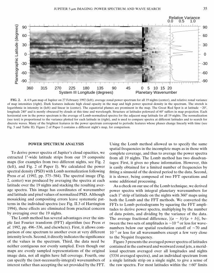
FIG. 2. A 4.9-em map of Jupiter on 27 February 1992 (left), average zonal power spectrum for all 19 nights (center), and relative zonal varianceof map intensities (right). Dark features indicate high cloud opacity in the map and high power spectral density in the spectrum. The stretch islogarithmic in intensity in (left) and linear in (center). The equatorial plumes are prominent in the map. The Great Red Spot is at latitude 2208,longitude 2408 and is mostly obscured by clouds at this time and wavelength. Structure at latitudes poleward of 608 suffers in map projection. Eachhorizontal row in the power spectrum is the average of Lomb-normalized spectra for the adjacent map latitude for all 19 nights. The normalization(see text) is proportional to the variance plotted for each latitude in (right), and is used to compare spectra at different latitudes and to search fordiscrete waves. Many of the brightest features in the power spectrum correspond to periodic features whose phases change linearly with time (seeFig. 5 and Table II). Figure 2 of Paper I contains a different night’s map, for comparison.

POWER SPECTRUM ANALYSIS Using the Lomb method allowed us to specify the samespatial frequencies in the incomplete maps as in those with

To derive power spectra of Jupiter’s cloud opacities, we complete coverage, and thus to average the power spectraextracted 18-wide latitude strips from our 19 composite from all 19 nights. The Lomb method has two disadvan-maps (for examples from two different nights, see Fig. 2 tages: First, it gives no phase information. However, this(left), and Fig. 2 of Paper I). We calculated the power is easily obtained for a limited number of frequencies byspectral density (PSD) with Lomb normalization following fitting a sinusoid of the desired period to the data. Second,Press et al. (1992, pp. 575–584). The spectral image (Fig. it is slower, being composed of two FFT operations and2, center) was produced by averaging the spectra at each some additional processing.latitude over the 19 nights and stacking the resulting aver- As a check on our use of the Lomb technique, we derivedage spectra. This image has coordinates of wavenumber power spectra with integral planetary wavenumbers forand latitude and pixel values of normalized PSD. Although each 18 strip of latitude on the nights with 3608 maps usingmosaicking and compositing errors leave systematic pat- both the Lomb and the FFT methods. We converted theterns in the individual spectra (see Fig. II.3 of Harrington FFTs to Lomb periodograms by squaring the FFT ampli-1994), these effects are eliminated from practical concern tudes to derive power spectra, multiplying by the numberby averaging over the 19 nights. of data points, and dividing by the variance of the data.

The Lomb method has several advantages over the sim- The average fractional difference, u(a 2 b)/(a 1 b)u, be-ple fast Fourier transform (FFT) algorithm (see Press et tween the two sets of amplitudes is p1026 or less for wave-al. 1992, pp. 496–536, and elsewhere). First, it allows com- numbers below our spatial resolution cutoff of p70 andparison of one spectrum to another even at very different 1023 or less for all wavenumbers except a few very closeintensity levels. Second, it directly indicates the significance to the Nyquist frequency.of the values in the spectrum. Third, the data need be Figure 3 presents the averaged power spectra of latitudesneither contiguous nor evenly sampled. Even though our contained in the eastward and westward zonal jets, a merid-maps are evenly sampled representations of the original ional spectrum averaged over all longitudes and nightsimage data, not all nights have full coverage. Fourth, one (5334 averaged spectra), and an individual spectrum fromcan specify the (not-necessarily-integral) wavenumbers of a single latitude strip on a single night, to give a sense of

the raw spectra. For most latitudes within the 6608 limitsinterest rather than accepting the set provided by the FFT.


Westward Jet Average

1 10 100Planetary Wavenumber

10-3

10-2

10-1

100

101

102

Pow

er S

pect

ral D

ensi

ty

Eastward Jet Average


10-3

10-2

10-1

100

101

102

Pow

er S

pect

ral D

ensi

tyAverage over System III Longitude


10-3

10-2

10-1

100

101

102

Pow

er S

pect

ral D

ensi

ty

Latitude 0, 22 March 1992


10-3

10-2

10-1

100

101

102P

ower

Spe

ctra

l Den

sity

FIG. 3. Power spectrum averages. Power law fits in the indicated wavenumber ranges are above the data. Dashes plot the theoretical 2D energyand enstrophy cascade slopes. Mitchell and Maxworthy (1985) measured slopes of 21.3 (a portion is plotted with dots) and 23 in wind velocitydata, but with a breakpoint near wavenumber 45. The lower left plot is a meridional spectrum. It has similar trends to the zonal spectra, but witha superposed pattern of peaks. This plot uses the same spatial wavenumbers as the zonal plots (but see text). The lower right plot is from a singlenight at a single latitude, to show the quality of unaveraged spectra. See text for discussion of errors. At high wavenumbers, the zonal spectraconfidently follow power laws with slopes near 23, but discrete waves disrupt the linearity of the low-wavenumber spectra. See Table I for numericalfit values.

of good map projection, plotting the logarithm of the power noise and reveals the underlying structure more clearly.The meridional spectrum is provided to illustrate the spec-spectrum against the logarithm of the planetary wavenum-

ber (m) reveals a slope near 20.8 at low wavenumbers tral behavior of the zonal intensity including the cloudbelts. The belt–zone intensity variation is characterizedwith superposed discrete features, a steeper slope at wave-

numbers higher than p25 that is relatively linear, and a not by a single peak but rather by a series of steadilyweakening peaks.low-intensity tail starting at m p 70, whose slope and curva-

ture vary. Averaging over latitudes significantly reduces Table I reports fits to linear ranges of the spectra aver-


TABLE IPower Law Fits to Regions of the Spectra

a Confidences for low-wavenumber fit are all less than 0.05%. These fits are presented to characterizethe first-order behavior of the region, not to establish power laws.

b Longitude range stated, same spatial wavenumbers as in zonal fits.

aged over regions noted in the table. We evaluated the (PSF) corresponds to about 28 on Jupiter. This is roughlyequivalent to the smoothing performed by Travis to elimi-point between the two slopes by eye and found that in

most of the narrow latitude ranges the breakpoint was nate an aliasing problem from abrupt cloud edges in hisdata for the Earth. We found that smoothing the data towithin one or two wavenumbers of 26. We adopted this

value and terminated the fits two wavenumbers away. Each reduce noise also reduced our sensitivity at high wavenum-bers. We have therefore not further smoothed our data,average includes only those wavenumbers within the reso-

lution limit, which varies with latitude (see below). The nor have we rebinned their intensities. We also take linearrather than log averages. Although Travis averages in thehighest wavenumbers have representation only from the

lowest latitudes in an average, hence the growth of error log, the Fourier transform is linear and other workers (e.g.,Julian and Cline 1974, Mitchell 1982, and Mitchell andbars at the highest wavenumbers. The upper limit for the

high-wavenumber fit is the highest wavenumber resolved in Maxworthy 1985) do not mention log averaging. Theseaverages presume that the spectra are constant over thethe average. The width of our image point-spread function


19 nights and within the averaging region, which is a predic- their slopes. We present the low-wavenumber and meridio-nal fits only to characterize the first-order behavior of thetion of cascade theory for inertial subranges (see Back-

ground, above). spectra and do not draw any further conclusions from them.Note that the spectral breakpoint is close to the locationWe wish to search for waves and establish power laws

in the presence of potentially many types of signals. We (PSD 5 1) where the Lomb normalization predicts signifi-cant wave activity. In a region with waves the inertial as-use the variance of the data to place an upper bound on

random meteorological noise. Because the variance of a sumption of cascade theory breaks down, and we do notexpect simple power laws. See Wave Search, below, fordata set consisting of Gaussian random noise is propor-

tional to the standard deviation of its exponentially distrib- statistics on some individual wavenumbers over time.Three dynamical parameters potentially affect the endsuted, white-noise power spectrum, the Lomb periodogram

is normalized according to the data’s variance. Significant of the actual subranges. These are the radius of deforma-tion, the Rhines cascade-arrest scale, and the Rossby num-peaks in the data appear at PSD levels larger than unity,

so one assigns uncertainties of unity to the points in the ber. In addition, image quality alters the observed spectrumat high wavenumbers. Figure 4 shows these parametersindividual power spectra.

Observational error in these data is small, about 1/200 and where they appear relative to each other and the data.First, image quality (atmospheric ‘‘seeing,’’ optical dif-of the typical zonal variance. Further, it is dominated by

nearly constant background and array readout noise fraction, telescope tracking errors, etc.) places a fundamen-tal limit on how small an object the images resolve. Thesources rather than by the variable photon statistics of

Jupiter. Thus, these uncertainties propagate into the power full-width at half-maximum (FWHM) of the PSF in theimages is typically 0.50–0.750 and has a greater effect awayspectrum as a low level of nearly white noise. Of greater

concern are the effects of mosaicking and mapping errors from the sub-Earth point on the planet than near it. Seeingacts much like a Gaussian filter. To find its effect on power(see Paper I). Our composite images rarely contain pixels

more than 458 from the central meridian and never use spectra, we convolved sine curves with Gaussian curves ofthe appropriate width. We find that at Jupiter’s equator apixels further than 608 away. If we simulate gross

mosaicking/mapping errors by shifting 25% of the dataset 0.750 FWHM PSF reduces the amplitude of the powerspectrum at planetary wavenumber 60 by 50%. As latitudeby 18 (much more than we expect for such a large fraction

of the data), the fractional leakage to the adjacent wave- increases, this limit moves to lower wavenumbers, as shownin Fig. 4A. The 0.750 FWHM PSF corresponds to p2500number is about 1.6 3 1025 at wavenumber 1, 0.15% at

wavenumber 10, 1.4% at wavenumber 30, and 4.2% at km at Jupiter’s distance, which allows us to be sensitiveto values of the Rossby deformation radius, Ld , as smallwavenumber 50. Leakages two wavenumbers away are

about half these values. Two 18 shifts in opposite directions, as 2500 km/2f P 400 km.the second representing about 10% of the data, yield num- Second, if a cascade reaches sufficiently low wavenum-bers well under twice these values. For our power spectra, bers, energy can propagate away in Rossby waves. Thisthese effects are all tiny compared to the variance. When energy sink destroys a cascade’s inertial character and ter-we average over 19 nights and over a range of latitudes, minates the linear portion of its power spectrum. The lowereven the variance effects of a single night are made small. limit wavenumber for turbulence in geostrophic systems

Since we are fitting in the log, we have weighted the is the Rhines cascade-arrest scale (Rhines 1979, Shep-uncertainties by 1/PSD. We calculate the confidence (prob- herd 1987),ability that x 2 as poor as that calculated from the datawould occur by chance from the fitted power law) to testthe presumption of quiescent spectrum as well as the valid- kb 5 ! b

2U, (1)

ity of the power law models of the fits. The high-wavenum-ber fits, with one exception, all have moderate to excellent

where U is the horizontal wind velocity scale, b 5 2Vconfidence (some greater than 99.95%), so we concludecos(l)/R is the local derivative of the vertical componentthat the underlying behavior is in fact linear in this sub-of the Coriolis parameter, f 5 2V sin(l), with respect torange.latitude l, V is the planetary rotation rate, and R is theThe confidences at low wavenumbers and in both meridi-planetary radius. By using the zonal-wind profile measuredonal subranges are all less than 0.05%, indicating that theby Limaye (1986), and taking U to be half the range ofconstant power law model is not valid here. In an effortwind speeds between minima in the profile, we find the kbto find a linear region corresponding to the 25/3 energyplotted in Fig. 4B.cascade, we attempted fits in the low-wavenumber region

Although the atmosphere could hypothetically supportstarting at wavenumbers as high as 12 (higher than thosewaves with wavenumbers higher than the Rhines scale, ourof all wave candidates in Table II). Those fits still had

vanishing confidence and also had a large distribution in average spectrum does not show any significant discrete



-90

-60

-30

0

30

60

90P

lane

togr

aphi

c La

titud

e (d

egre

es)

Image Resolution


-90

-60

-30

0

30

60

90

Pla

neto

grap

hic

Latit

ude

(deg

rees

)

Rhines Cascade-Arrest Scale


-90

-60

-30

0

30

60

90

Pla

neto

grap

hic

Latit

ude

(deg

rees

)

Ld=3000, 2000, 1000km


-90

-60

-30

0

30

60

90

Pla

neto

grap

hic

Latit

ude

(deg

rees

)

Rossby Number = 1

FIG. 4. Scales that affect the observed spectra as a function of latitude. (A) shows the effect of image resolution on our sensitivity to highwavenumbers; because a circle of longitude is smaller at high latitude, planetary wavenumber sensitivity decreases there. (B) shows the Rhinescascade-arrest scale (see Eq. (1)) plotted over the spectral image of Fig. 2, to show how the plotted limit relates to the region of the data wherediscrete waves appear (see Fig. 3 for overall spectral appearances). (C) shows the location of three possible values for the deformation radius, Ld ;from left to right these are 3000, 2000, and 1000 km at 458 latitude, assuming gravity-wave speed is independent of latitude. (D) shows the wavenumberwhere the Rossby number equals unity; values are smaller poleward of the wedge and larger within it. See text for further discussion.

features at higher wavenumbers, signifying a lack of high- instability enter the power spectra (Pedlosky 1987, p. 521).Ld is related to the density stratification via Ld f P NH 5frequency periodic structure. We can therefore conclude

that the effect on cloud opacities from high-frequency forc- c, where N is the Brunt-Vaisala frequency, H is the verticalscale height, c is the phase speed of the fastest gravity-ing—an example might be highly structured convective

overshooting at the base of the stable atmosphere—is rela- wave mode, and the approximation is valid away from theequator on Jupiter. The midlatitude terrestrial data in Fig.tively weak or nonexistent. Turbulence, not waves, appears

to dominate at the smallest scales, which is quite rea- 1 (left) show this energy input at n 5 6. Ld for Jupiter isthought to be p3000 km in the stratosphere (Conrath etsonable.

Third, the radius of deformation, Ld , is the principal al. 1981) and p1800 km in the troposphere (Hammel etal. 1995). Ld enters the equations in the context of anlength scale at which fluctuations produced by baroclinic


inverse wavenumber, i.e., k2 1 l2 1 L22d , and we have Our results are partly similar to the conclusions of Mitch-

ell (1982) and Mitchell and Maxworthy (1985). They de-plotted three possible values in Fig. 4C. The curves in Fig.4C are derived from Eq. 3 of Ripa (1983): rived horizontal wind vectors from pairs of Voyager images

to calculate the kinetic energy spectrum directly, a distinctadvantage over the present work. Their power law expo-

Ld 52c

u f u 1 Ïf 2 1 2bc. (2) nents are 21.3 and 23, with a breakpoint at planetary

wavenumber p45. However, the intrinsic uncertainty inwind measurements leads to very noisy spectra. These

Lacking definitive information, we take three values fornumbers appear in final form without error estimates, so

Ld (1000, 2000, and 3000 km) at a latitude of 458 and plotwe cannot quantitatively compare results, but Fig. 3 shows

the curves passing through them, assuming constant c. Thethese slopes next to our spectra. We agree with the 23

shape of these curves would differ from those presentedslope, though it is clear that our breakpoint is not consistent

here if c were not constant.with their location, unless that location has a large error

Finally, the quasi-geostrophic approximation, which isbar. We note that until we compared many nights of data,

involved in the reduction to quasi-two-dimensional fluidwe were unable to detect the discrete waves that disrupt

dynamics, breaks down ifany low-wavenumber power law in our spectra (see below).It may be the same effect that yields a first-order behaviorof 21.3 rather than 25/3 in their data. The preliminary« 5

UfL

. 1, (3)error analysis of Mitchell (1982) was done in such a waythat it might not have detected the influence of discretewaves.where « is the Rossby number and L is the horizontal

length scale. Figure 4D shows the wavenumber corre-sponding to the length scale where « 5 1 on Jupiter using WAVE SEARCHthe same U as for kb. We would not expect wavenumbershigher than this value at a given latitude to exhibit the 23 The only atmospheric waves long enough to be well

resolved by our data are Rossby waves. We envision twoslope of an enstrophy cascade in quasi-two-dimensionalturbulence. means by which a Rossby wave could manifest itself in

our data. First, since the zonal winds correspond well withThese limits are all estimates rather than hard cutoffs,and a factor of 2 in accuracy is the best we can do for the banded cloud structure (Limaye 1986), a Rossby wave

near the edge of a bright or dark band could give rise to amost of them (the image quality limit is somewhat betterthan this). meridional undulation in the location of the edge. Second,

since the dynamical thickness of the weather layer con-As discussed earlier, the high-wavenumber fits in TableI have power laws near 23, which mimics what would be taining a Rossby wave varies with the phase of the wave,

the local cloud thickness could vary as well, giving riseexpected in a kinetic energy spectrum if enstrophy werecascading between wavenumbers p25 and p60. Our data to an undulating light pattern at a given latitude. Such

oscillations are given by the perturbation streamfunctionreveal a tendency for the slopes to be steeper at higherlatitudes. The low latitudes contain more eastward than in the dispersion relation derivation of Harrington (1994,

Part II, Appendix D).westward motion, and as a result the westward jet averageis steeper than the eastward jet average. Studying the undulations of the cloud belts at first ap-

pears promising. Jupiter’s banded cloud patterns provideIf the empirical correspondence of Travis (1978) is tobe believed, then our fits indicate a lack of energy input many regions where clouds end abruptly, so any Rossby

waves strong enough to influence these cloud bordersbetween wavenumbers p25 and p60 at most latitudes.Any significant added energy in this range would cause an should show up as wiggles in the otherwise-straight inter-

face between a cloud belt and a clear zone. There areupscale energy cascade with a 25/3 power law, whichwould disrupt the observed enstrophy cascade. Thus, the other effects that would cause such undulations, however,

including passing long-lived vortices and the spread of con-highest discrete wavenumber at which significant energyenters the atmosphere is near 25 under this interpretation. vected material. Errors in mosaicking and finding the plan-

etary center would further contaminate an edge-locationThe most likely candidate for the source is baroclinic insta-bility, and this would indicate that 1/Ld is somewhere near analysis. A wave would also need to perturb a cloud belt

by at least one degree of latitude to be seen clearly. Becauseplanetary wavenumber 25, corresponding to Ld P 2100 kmat 458. We do not see clear evidence for an inertial energy of these difficulties, we followed the second approach,

looking for wave-like intensity variations at a given lat-cascade as the low-wavenumber power laws are almostnever close to the predicted 25/3 and the confidence level itude.

The power spectra show many discrete features, primar-of linear fitting is low.


Latitude -50, Wavenumber 5

620 640 660 680 700 720 740Julian Day - 2448000

-100

-50

0

50

100P

hase

(de

gree

s S

yste

m II

I)

Latitude -46, Wavenumber 3

620 640 660 680 700 720 740Julian Day - 2448000

-100

0

100

200

300

Pha

se (

degr

ees

Sys

tem

III)

FIG. 5. Linear fits to the best and (nearly) worst wave candidates in Table II (the worst fit has a high velocity that makes the plot difficult toread). Some periodic features in the data propagate with near-linear speeds, making them good wave candidates. The data on each plot are repeatedvertically at intervals of one period to show the separation of the data near the center fitted line from the equally valid data plotted above andbelow. Of the 384 strong periodic features in the data, only 46 show linear behavior comparable to or better than that of the right panel. Most ofthese are repetitions of broad features at adjacent latitudes; there are about 24 separate phenomena reported in the table. Some of these appearto follow known features from visible-light images but many remain unidentified.

ily at low wavenumbers. The Lomb normalization tells us vents the naıve use of linear fitting; some of these datacontain enough phase cycles that they appear random whenthe likelihood that a given feature represents an actual

periodic signal in the data, as opposed to random noise. plotted in System III. We therefore iteratively fit the datain a range of rotational reference frames and phase offsets.Equations 13.8.7 and 13.8.8 of Press et al. (1992) state

the probability of a power spectrum containing a Lomb- A fit was good if it had less than 408 root-mean-square(RMS) scatter relative to the period (i.e., this num-normalized value greater than z by random chance (theber would be 208 of planetary phase for an m 5 2 wave,false-alarm probability)58 of planetary phase for an m 5 8 wave, etc.). By fitting

P(.z) 5 1 2 (1 2 e2z)M P Me2z, (4) the data in the frame of a good fit, we converged to thebest fit, usually in one or two iterations. If a candidate

where M is the number of independent wavenumbers and wave did not have a frame with better than 408 scatter, wethe approximation is valid for small probabilities. The Ny- doubled the search resolution in both speed and phase.quist theorem (Eq. 13.8.2 of Press et al.) says M 5 180 for The range of speeds searched was 6(1.5 uuu 1 15 m/sec),our 18 bins. We wish to expect not to be fooled even once where u is zonal wind speed. We gave up our search whenin the entire dataset, and so we select a cutoff value for z the resolution reached 5 m/sec in the wave speed. Givensuch that we expect a false alarm only once in at least the uneven spacing of our 19 nights, finding differenttwice our 121 3 19 different spectra. Our cutoff is thus speeds that fit the same data well is unlikely below a rela-z 5 13.6. tively tight cutoff RMS. We discovered one such candidate

There were 384 locations in our averaged power spec- with two fits of similar quality at RMS P558, so Table IItrum image between 6608 latitude whose values were presents only those candidates whose RMS is below 408.greater than our cutoff. We fit sinusoids in the original There is some redundancy in Table II, since some fea-maps for all 19 nights at the corresponding latitudes and tures cross more than 18 of latitude. We consider all candi-wavenumbers and derived the amplitude and phase of each dates at the same wavenumber, similar speeds, and adja-wave candidate. Image-processing error exceeds the for- cent latitudes to be due to the same cause. There are thusmal error of the phase fit, so we assigned a phase uncer- about 24 different physical phenomena in the table. Tabletainty of 1.5 pixels converted to the appropriate angle for II additionally shows the zonal wind (from Limaye 1986)a given latitude plus the per-mosaic rotation uncertainty at the latitude of a wave candidate, the fitted speed dividedof the particular night (see Paper I). by the wind, the mean and standard deviation of Lomb-

Long-lived waves propagate at a constant speed, so it normalized PSD over the 19 nights, and the number ofwould be appropriate to fit a line to the derived phases those nights where the PSD was greater than our cutoff

of 13.6.(see Fig. 5). However, the cyclic nature of phase data pre-


By searching visually in the map image of 22 March, we ture at 2358 latitude, 1208 away in longitude. At the higherwavenumbers, some of the candidates are due to sequenceshave a preliminary identification for some of the candi-

dates. The wavenumber 2–3 candidates are all in regions of individual features that are evenly spaced, or combina-tions of these and brighter areas of their latitude. Finally,with clusters of brighter features spaced relatively evenly

in longitude. The clustering is more evident in the north the last candidates are clearly related to the equatorialplumes, being located at latitudes crossed by a sequencethan in the south. The wavenumber 3 candidate at 2308

is very likely related to the lower edge of the GRS; the of diagonal brightenings. We were unable to identify causesfor some candidates in the table. We leave for future workpower spectra there show continua of power. Wavenumber

3 probably propagates linearly because of the bright fea- the determination of why there are periodic, propagating


brightenings at some latitudes. It is worth noting, again linearly in time. Some of these are due to well-knownfeatures, such as the equatorial plumes. Others raise thewithout explanation, that the lower wavenumber features

at latitudes near 2478 move with a significant fraction of question of their underlying causes, which we leave forfuture work. We note that only by incorporating data fromthe zonal wind, but the higher wavenumber features are

all stationary in System III. This precludes a simple Rossby all 19 nights of observation and using the Lomb methodwere we able to identify any propagating waves at all. Ourwave interpretation. This description of features is tenta-

tive and awaits a more thorough comparison to data at preliminary analysis of the six nights with full longitudecoverage (Harrington 1994) did not identify any waves.other wavelengths.

With two possible exceptions (wavenumber 3 at 2588 Although the appearance of Jupiter did not change ona large scale in our 99 days of observation, its appearanceand 2308 and wavenumber 5 at 2518 and 2328), we did

not find pairs of candidates at the same wavenumber and at 4.9 em has been markedly different in other years. Forexample, sometimes the rim of the GRS is very bright andspeed but at different latitudes. A population of such fea-

tures would support the banana-cell convection of Hart et the entire latitude band of the GRS is among the brightestand most active on the planet, rather than the darkest. Ital. (1986a,b). If the convection underlying the atmosphere

follows the banana-cell pattern, any resulting variation in would be interesting to calculate spectra in the GRS regionwithout an obscuring cloud band. It is possible that thecloud opacity is too weak for us to detect.dynamics that cause changes in cloud distribution couldalso excite wave activity, so it may be worthwhile to per-CONCLUSIONSform a search similar to this one when Jupiter’s appearanceis changing.Our power spectra show that Jupiter’s cloud opacities

follow a power law at planetary wavenumbers above p25;the exponent is near 23. Variation among latitudes is ACKNOWLEDGMENTSsometimes larger than the formal errors of the fits, but not

We thank P. Stone, A. Ingersoll, F. M. Flasar, J. L. Mitchell, R.out of line with that reported in the literature for the EarthPierrehumbert, and two anonymous referees for comments and helpful(Julian and Cline 1974). The spectra away from the equatordiscussions. Analysis work was funded in part by NASA Planetary Atmo-

are steeper than those near the equator. Although the spheres Grant NAGW-2956. A portion of this work was performed whiletheory of atmospheric turbulence has not yet been con- J.H. held a National Research Council-NASA Goddard Space Flight

Center Research Associateship.nected to cloud opacity spectra, our power laws approxi-mate the k23 enstrophy cascade spectrum at high wavenum-bers. There is prior observational evidence (Travis 1978) REFERENCESthat cloud opacity spectra mimic kinetic energy spectra, in

ACHTERBERG, R. K., AND F. M. FLASAR 1996. Planetary-scale thermalwhich the enstrophy cascade is found. If this is the case,waves in Saturn’s upper troposphere. Icarus 119, 350–369.

then our results indicate that there is no significant energyALLISON, M. 1990. Planetary waves in Jupiter’s equatorial atmosphere.

input scale larger than planetary wavenumber p25, since Icarus 83, 282–307.that would cause an upscale energy cascade with a 25/3 ALLISON M., D. A. GODFREY, AND R. F. BEEBE 1990. A wave dynamicalspectrum and would disrupt the power law we observe. interpretation of Saturn’s polar hexagon. Science 247, 1061–1062.We believe it likely that the top of the 23 power law BATCHELOR, G. K. 1959. Small-scale variation of convoluted quantities

like temperature in turbulent fluid Part 1. General discussion and therange is associated with Ld , the presumed input scale ofcase of small conductivity. J. Fluid Mech. 5, 113–133.baroclinic instability. Although there is not a strong peak

BEEBE, R. F., A. P. INGERSOLL, G. E. HUNT, J. L. MITCHELL, ANDat this wavelength, as there is for the Earth’s northernJ. P. MULLER 1980. Measurements of wind vectors, eddy momentumhemisphere, detecting it at all suggests that local baroclinictransports, and energy conversions in Jupiter’s atmosphere from Voy-

instability is potentially a significant process on Jupiter. If ager 1 images. Geophys. Res. Lett. 7, 1–4.this is the case, then the corresponding value for Ld at 458 BEER, R., AND F. W. TAYLOR 1973. The abundance of CH3D and thelatitude is p2100 km. D/H ratio in Jupiter. Astrophys. J. 179, 309–327.

The first search for planetary-scale waves on Jupiter in CHARNEY, J. G. 1971. Geostrophic turbulence. J. Atmos. Sci. 28, 1087–1095.5-em data, conducted by Magalhaes et al. (1989, 1990) and

based on rasterizing Voyager IRIS data, did not detect CONRATH, B. J., P. J. GIERASCH, AND N. NATH 1981. Stability of zonalflows on Jupiter. Icarus 48, 256–282.waves. That study did find periodic thermal features in the

DANILOV, S. D., F. V. DOLZHANSKII, AND V. A. KRYMOV 1994. Quasi-upper troposphere and both it and the studies by Demingtwo-dimensional hydrodynamics and problems of two-dimensional tur-et al. (1989) and Orton et al. (1991) detected slowly movingbulence. Chaos 4, 299–304.

thermal features in the stratosphere. Significant improve-DEMING, D., M. J. MUMMA, F. ESPENAK, D. E. JENNINGS, T. KOSTIUK,

ment in spatial and temporal resolution over the spacecraft G. WIEDEMANN, R. LOEWENSTEIN, AND J. PISCITELLI 1989. A searchstudy have enabled us to report about 24 separate periodic for p-mode oscillations of Jupiter: Serendipitous observations of non-

acoustic thermal wave structure. Astrophys. J. 343, 456–467.variations in tropospheric cloud opacity that propagate


Atmosphere. JPL Publication 82-34, Jet Propulsion Laboratory, Pasa-DOWLING, T. E. 1995. Dynamics of jovian atmospheres. Ann. Rev. Fluiddena, CA.Mech. 27, 293–334.

MITCHELL, J. L., AND T. MAXWORTHY 1985. Large-scale turbulence inDOWLING, T. E., AND A. P. INGERSOLL 1989. Jupiter’s Great Red Spotthe jovian atmosphere. In Turbulence and Predictability in Geophysicalas a shallow water system. J. Atmos. Sci. 46, 3256–3278.Fluid Dynamics and Climate Dynamics, pp. 226–240. Tipografia Com-GIERASCH, P. J., A. P. INGERSOLL, AND D. POLLARD 1979. Baroclinicpositori, Bologna, Italy.instabilities in Jupiter’s zonal flow. Icarus 40, 205–212.

ORTON, G. S., A. J. FRIEDSON, J. CALDWELL, H. B. HAMMEL, K. H.GODFREY, D. A. 1988. A hexagonal feature around Saturn’s north pole.BAINES, J. T. BERGSTRALH, T. Z. MARTIN, M. F. MALCOM, R. A. WEST,

Icarus 76, 335–356.W. F. GOLISCH, D. M. GRIEP, C. D. KAMINSKI, A. T. TOKUNAGA,

HAMMEL, H. B., R. F. BEEBE, A. P. INGERSOLL, G. S. ORTON, J. R. MILLS, R. BARON, AND M. SHURE 1991. Thermal maps of Jupiter: SpatialA. A. SIMON, P. CHODAS, J. T. CLARKE, E. DE JONG, T. E. DOWLING, organization and time dependence of stratospheric temperatures, 1980J. HARRINGTON, L. F. HUBER, E. KARKOSCHKA, C. M. SANTORI, A. to 1990. Science 252, 537–542.TOIGO, D. YEOMANS, AND R. A. WEST 1995. HST imaging of atmo- PEDLOSKY, J. 1987. Geophysical Fluid Dynamics, 2nd ed. Springer Verlag,spheric phenomena created by the impact of Comet Shoemaker-Levy New York.9. Science 267, 1288–1296. PIERREHUMBERT, R. T. 1992. Spectra of tracer distributions: A geometric

HARRINGTON, J. 1994. Planetary Infrared Observations: the Occultation approach. In Nonlinear Phenomena in Atmospheric and Oceanic Sci-of 28 Sagittarii by Saturn and the Dynamics of Jupiter’s Atmosphere. ences (G. Carnevale and R. T. Pierrehumbert, Eds.), pp. 27–46.Doctoral thesis in Planetary Science, MIT. Springer Verlag, New York.

HARRINGTON, J., T. E. DOWLING, AND R. L. BARON 1996. Jupiter’s tropo- PIERREHUMBERT, R. T. 1994. Tracer microstructure in the large-eddyspheric thermal emission I: Observations and techniques. Icarus 124, dominated regime. Chaos Solitons Fractals 4, 1091–1110.22–31. PRESS, W. H., S. A. TEUKOLSKY, W. T. VETTERLING, AND B. P. FLANNERY

1992. Numerical Recipes in C: The Art of Scientific Computing, 2nd ed.HART, J. E., G. A. GLATZMAIER, AND J. TOOMRE 1986a. Space-laboratoryCambridge Univ. Press, Cambridge, UK.and numerical simulations of thermal convection in a rotating hemi-

spherical shell with radial gravity. J. Fluid Mech. 173, 519–544. RHINES, P. B. 1979. Geostrophic turbulence. Ann. Rev. Fluid Mech. 11,401–441.HART, J. E., J. TOOMRE, A. E. DEANE, N. E. HURLBURT, G. A. GLATZ-

RIPA, P. 1983. General stability conditions for zonal flows in a one-layerMAIER, G. H. FICHTL, F. LESLIE, W. W. FOWLIS, AND P. A. GILMAN

model on the b-plane or the sphere. J. Atmos. Sci. 126, 463–489.1986b. Laboratory experiments on planetary and stellar convectionSADA, P. V., R. F. BEEBE, AND B. J. CONRATH 1996. Comparison ofperformed on Spacelab 3. Science 234, 61–64.

the structure and dynamics of Jupiter’s Great Red Spot between theJULIAN, P. R., AND A. K. CLINE 1974. The direct estimation of spatialVoyager 1 and 2 encounters. Icarus 119, 311–335.wavenumber spectra of atmospheric variables. J. Atmos. Sci. 31, 1526–

SAFFMAN, P. G. 1971. On the spectrum and decay of random two-dimen-1539.sional vorticity distributions at large Reynolds numbers. Stud. Appl.KUNDE, V., R. HANEL, W. MAGUIRE, D. GAUTIER, J. P. BALUTEAU, A.Math. 50, 377–383.

MARTEN, A. CHEDIN, N. HUSSON, AND N. SCOTT 1982. The troposphericSHEPHERD, T. E. 1987. Rossby waves and two-dimensional turbulence ingas composition of Jupiter’s north equatorial belt (NH3 , PH3 , CH3D,

a large-scale zonal jet. J. Fluid Mech. 183, 467–509.GeH4 , H2O) and the jovian D/H isotopic ratio. Astrophys. J. 263,TERRILE, R. J. 1978. High Spatial Resolution Infrared Imaging of Jupiter:443–467.

Implications for the Vertical Cloud Structure from Five-Micron Mea-LIMAYE, S. S. 1986. Jupiter: New estimates of the mean zonal flow at the

surements. Doctoral thesis, California Institute of Technology.cloud level. Icarus 65, 335–352.

TESSIER, Y., S. LOVEJOY, AND D. SCHERTZER 1993. Universal multifrac-MAGALHAES, J. A., A. L. WEIR, B. J. CONRATH, P. J. GIERASCH, AND tals: Theory and observations for rain and clouds. J. Appl. Meteorol.

S. S. LEROY 1989. Slowly moving thermal features on Jupiter. Nature 32, 223–250.337, 444–447. TRAVIS, L. D. 1978. Nature of the atmospheric dynamics on Venus from

MAGALHAES, J. A., A. L. WEIR, B. J. CONRATH, P. J. GIERASCH, AND S. S. power spectrum analysis of Mariner 10 images. J. Atmos. Sci. 35, 1584–LEROY 1990. Zonal motion and structure in Jupiter’s upper troposphere 1595.from Voyager infrared and imaging observations. Icarus 88, 39–72. WEST, R. A., D. F. STROBEL, AND M. G. TOMASKO 1986. Clouds, aerosols,

and photochemistry in the jovian atmosphere. Icarus 65, 161–217.MITCHELL, J. L. 1982. The Nature of Large-Scale Turbulence in the jovian

Documents

Jupiter's Tropospheric Thermal Emission. II. Power Spectrum Analysis and Wave Search