Jumps and stochastic volatility in crude oil futures

prices using conditional moments of integrated volatility

Christopher F Bauma,b,1, Paola Zerillic

aDepartment of Economics, Boston College, Chestnut Hill, MA 02467 USAbDepartment of Macroeconomics, DIW Berlin, Mohrenstraße 58, 10117 Berlin

cDepartment of Economics and Related Studies, University of York, York YO10 5DD,UK

Abstract

We evaluate alternative models of the volatility of commodity futures pricesbased on high-frequency intraday data from the crude oil futures marketsfor the October 2001–December 2012 period. These models are implementedwith a simple GMM estimator that matches sample moments of the realizedvolatility to the corresponding population moments of the integrated volatil-ity. Models incorporating both stochastic volatility and jumps in the returnsseries are compared on the basis of the overall fit of the data over the fullsample period and subsamples. We also find that jumps in the returns seriesadd to the accuracy of volatility forecasts. (JEL: G13, Q41)

Key words: stochastic volatility, commodity futures prices, crude oilfutures

Email addresses: baum@bc.edu (Christopher F Baum), paola.zerilli@york.ac.uk(Paola Zerilli)

1Corresponding author.

October 13, 2014

1. Introduction

The volatility of commodity futures prices has become a topic of increas-

ing interest in recent years for academic researchers, practitioners and those

involved with the regulation of derivatives markets. Many commodity fu-

tures markets have become increasingly ‘financialized’ over the past decade

as financial firms with no inherent exposure to the commodity have adopted a

strategy of portfolio diversification into commodity futures as an asset class.

Although this trend has affected many commodity futures markets, it has

had a marked impact on one of the most important markets: that for deriva-

tives of crude oil, which is now the most heavily traded commodity futures

contract by volume. Crude oil, as a key global commodity, has experienced

considerable price level variation in the boom preceding the global financial

crisis in 2008 and the ensuing Great Recession. A major oil price shock in

2008 was caused by constraints on the production of crude oil paired with

low elasticity of demand (for details, see Hamilton (2009) and Kilian (2009)).

This shock, while being caused by fundamentals, was clearly exacerbated by

financial speculation and ‘financialization’ of commodities. Variation in oil

price levels has been accompanied by wide variations in the volatility of re-

turns. In the futures markets, returns exhibit heavy tails, autocorrelation,

and volatility clustering, leading to significant challenges in modeling their

first and second moments.

Both the International Monetary Fund (IMF) and the Federal Reserve

Board (see Alquist et al. (2011) and IMF 2005 p. 67; 2007, p. 42) use futures

prices as the best available proxy for the market expectations of the spot

crude oil price.

Like many financial series, commodity futures prices are likely to exhibit

random-walk behavior. Such behavior in crude oil futures prices implies that

a model of prices or returns is not likely to beat the naıve model. How-

ever, even if returns are not forecastable, their volatility may be successfully

modeled. In this paper, we employ various models of stochastic volatility in

order to analyze the uncertainty of crude oil futures returns and to evaluate

the forecastability of their volatility. The empirical analysis makes use of

high-frequency (tick-by-tick) data from the futures markets, first aggregated

to 10-minute intervals during the trading day. The intraday variation is then

utilized to generate daily time series of prices, returns and realized volatility.

Our sample period of October 2001 to December 2012 is characterized by

high frequency fluctuations and fat tails. This is an appropriate setting for

our investigation of the role of jumps (modelled as extreme events). Before

performing any model estimation, we employ non-parametric methods to

identify the periods when these extreme events might have occurred. Our

empirical findings are in line with these test results indicating a very high

volatility during 2008.

The high frequency data allows us to test various models for oil futures

returns using a straightforward Generalized Method of Moments (GMM)

estimator that matches sample moments of the realized volatility to the cor-

responding population moments of the integrated volatility in the spirit of

Bollerslev and Zhou (2002). These models are then compared, in terms of

overall fit of the data and forecast accuracy statistics, over the full sample.

The model with stochastic volatility and jumps is also tested over a sub-

sample (January 2006–December 2012) to address structural stability (as in

1

Andersen, Benzoni and Lund (2002)). Key findings include the importance

of both jumps and stochastic volatility in oil futures returns and the apparent

unimportance of leverage as a modeled component.

The wider applicability of this method of estimation to other markets is

outside the scope of this paper, but an interesting topic for future research.

2. Review of the literature

Schwartz (1997), Schwartz and Smith (2000), Casassus and Collin-Dufresne

(2005) propose multi-factor models for energy prices where returns are only

affected by Gaussian shocks only, but constrain volatility to be constant.

Pindyck (2004) examines the volatility of energy spot and futures prices, es-

timating the standard deviation of their first differences. Askari and Khrich-

ene (2008) fit jump-diffusion models to futures on Brent crude oil. Schwartz

and Trolle (2009) propose a multifactor stochastic volatility model for pricing

futures and options on light sweet crude oil trading on the NYMEX. Using

daily data, they present evidence that taking account of stochastic volatility

improves pricing, but they consider the inclusion of jumps to be less impor-

tant. Vo (2009) estimates a multivariate stochastic volatility model using

daily data on the West Texas Intermediate (WTI) crude oil futures contracts

traded on the NYMEX and finds that stochastic volatility plays an important

role.

Larsson and Nossman (2011) find evidence for stochastic volatility and

jumps in both returns and volatility daily spot prices of WTI crude oil from

1989 to 2009.

The role of volatility as a measure of uncertainty of oil price futures is

2

stressed by Bernanke (1983), Pindyck (1991) and Kellogg (2010) who show

that this measure of uncertainty is extremely relevant for firms’ investment

decisions.

Our contribution lies in the use of the information on volatilty of oil

futures returns provided by high frequency, intra-day data while focusing on

the role of volatility as measure of variability and uncertainty of oil price

forecasts.

3. Data description

We exploit the distributional information embedded in high-frequency

(10-minute interval) intraday futures price quotations on crude oil in order

to test for the presence of stochastic volatility and jumps in crude oil futures

returns.

Light, sweet crude oil (West Texas Intermediate) began futures trading

on the New York Mercantile Exchange (NYMEX) in 1983 and is the most

heavily traded commodity future. Crude oil futures trade in units of 1,000

U.S. barrels (42,000 gallons), with contracts dated for 30 consecutive months

plus long-dated futures initially listed 36, 48, 60, 72, and 84 months prior

to delivery. Additionally, trading can be executed at an average differential

to the previous day’s settlement prices for periods of two to 30 consecutive

months in a single transaction. Crude Oil Futures are quoted in dollars and

cents per barrel.

The raw data used in this study are 10-minute aggregations of crude

oil futures contract transactions-level data provided by TickData, Inc. For

each 10-minute interval during the day trading session and for each traded

3

contract, the open, high, low, close prices are recorded, along with the volume

of trades in that interval. For the purpose of computing returns, the trading

session’s close price and the following trading session’s close price are used

to produce an estimated overnight (or over-the-weekend) return.

Industry analysts have noted that to avoid market disruptions, major

participants in the crude oil futures market roll over their positions from

the near contract to the next-near contract over several days before the near

contract’s expiration date. A continuous price series over contracts, which

expire monthly, is created by hypothetically rolling over a position from the

near contract to the next-near contract three days prior to expiration of the

near contract.

The returns series and the realized volatility measures are displayed in

Figure 1 and their descriptive statistics are given in Table 1. Both series

exhibit excess kurtosis, while the realized volatility series has a large skewness

coefficient. The Kolmgorov–Smirnov test for normality rejects its null for

both series, while the Shapiro–Francia test (1972) for normality concurs with

those judgements. The Box–Pierce portmanteau (or Q) test for white noise

rejects its null for both series. The daily returns series exhibits significant

ARCH effects at 1, 5, 10 and 22 lags, while no evidence of ARCH effects is

found in the realized volatility series.

4. Estimation method

Following Bollerslev and Zhou (2002), who use continuously observed

futures prices on oil, we build a conditional moment estimator for stochastic

volatility jump-diffusion models based on matching the sample moments of

4

realized volatility with population moments of integrated volatility. In this

context, as Andersen and Benzoni (2008) have suggested, realized volatility

serves as a non-parametric ex post estimate of the variation in returns. In

this paper, realized volatility is computed as the sum of high-frequency (10-

minute interval) intraday squared returns.

4.1. No-jump case

The returns on futures at time t over the interval [t− k, t] can be decom-

posed as

r (t, k) = lnFt − lnFt−k =

∫ t

t−kµ (τ) dτ +

∫ t

t−kσ (τ) dWτ

The quadratic variation or integrated variance, which coincide in the no-

jump case, can be expressed as

QV (t, k) = IV (t, k) =

∫ t

t−kσ2 (τ) dτ

In discrete time, the corresponding sample realized variance (RV) can be

described as

RV (t, k, n) =n·k∑j=1

r

(t− k +

j

n,

1

n

)2

RV (t, k, n) −→p IV (t, k) as n −→∞

where n is the sampling frequency of 33 intervals per day when we derive the

daily RV.

4.2. Integrated volatility and jumps

When we allow for discrete jumps, the returns on futures at time t over

the interval [t− k, t] can be decomposed as

5

r (t, k) = lnFt − lnFt−k

=

∫ t

t−kµ (τ) dτ +

∫ t

t−kσ (τ) dWτ +

∫ t

t−kx (τ) dN (λτ)

In this case, integrated variance and quadratic variation do not coincide:

IVjumps (t, k) =

∫ t

t−kσ2 (τ) dτ +

∑t−k≤s≤t

(x (s) dN (λs))2

= QV (t, k) +∑

t−k≤s≤t

(x (s) dN (λs))2

Barndorff-Nielsen and Shephard (2004) proposed the Realized Bipower

Variation as a consistent estimate of integrated volatility component in the

presence of jumps:

BV (t, k;n) = π2

∑n·ki=2

∣∣r (t− k + ikn, 1n

)∣∣ ∣∣∣r (t− k + (i−1)kn

, 1n

)∣∣∣

RV (t, k, n)−BV (t, k;n) −→ QV (t, k)− IV (t, k)

QV (t, k)− IV (t, k) =∑

t−k≤s≤t

(x (s) dN (λs))2

as n −→∞

4.3. Data filtering

Given the high autocorrelation of the square root of the realized variance

(RV) series, the analysis in this paper is performed on moving averages of

the daily realized volatility series, using arithmetic weights over the current

trading session and three previous trading sessions:

MA4RVt = 0.4RVt + 0.3RVt−1 + 0.2RVt−2 + 0.1RVt−3

6

As we can notice from Figure 2 and Figure 3 , the autocorrelation in the

first differences of the daily realized volatility is reduced significantly after

applying the moving average transformation to the data.

5. Estimation results

We estimated four forms of the stochastic model: the basic (SV) model,

the SV model incorporating leverage (in which the volatility is influenced

by the level of returns), (SVLev); the SV model incorporating jumps in the

returns process (SVJ), and the SV model incorporating both leverage and

jumps in the return process (SVLevJ). As we discuss below, there is no

empirical support for leverage, in that the parameter expressing the effect of

leverage is never significantly different from zero. Thus, we present here our

findings from the SV and SVJ models.

5.1. Stochastic Volatility model (SV)

We model the returns on futures on crude oil using the Heston (1993)

model. For simplicity, we set the drift of the log price equal to zero.2 This

choice is consistent with Alquist et al. (2011) who find that a reasonable

and parsimonious forecasting model for spot oil prices is the random walk

without drift.

2As Bollerslev et al. (2002) suggest, a drift could be easily introduced in the futuresreturns equation.

7

dpt = d ln(Ft)

=√VtdW1t

dVt = κ (θ − Vt) dt+ σ√VtdW2t

E (dW1tdW2t) = 0

In this model, there are two orthogonal Wiener processes, dW1t and dW2t,

driving the evolution of returns and volatility. Three estimated parameters

appear in the model: κ, θ and σ.

We estimated this model over the full sample, imposing the six moment

conditions implied by the model in the GMM procedure. As there are six

moment conditions and three estimated parameters, there are three overi-

dentifying restrictions that may be used to evaluate the model. As shown in

Table 3, all six moment conditions are in accordance with the data, and the

Hansen’s J statistic indicates that the overidentifying restrictions are valid.

The three estimated parameters of the model are very precisely estimated

and take on sensible values from an analytical perspective.

5.2. Stochastic Volatility model with jumps in returns (SVJ)

dpt = d ln(Ft)

=√VtdW1t + xdPoisson (λt)

dVt = κ (θ − Vt) dt+ σ√VtdW2t

E (dW1tdW2t) = 0

8

x ∼ N(0, σ2

x

)In this extended model, the same two orthogonal Wiener processes ap-

pear, augmented by a Poisson process that captures jumps in returns. This

gives rise to two additional parameters, λ and σx, governing the effects of the

jump process.

λ is the indicator of the frequency of the jumps: it tells us, on average,

how many times we have extreme events (jumps in this case for us are extreme

events) within the sample. It is the parameter of the Poisson counting process

that takes values:

{1 when an extreme event happens0 otherwise

The Normally distributed, mean zero random variable x represents the

magnitude of the jumps in returns, with the intensity of jumps controlled by

the σ2x parameter. The timing of jumps is a Poisson process, with parameter

λ representing the mean and variance of that process. For jumps in returns

to play a significant role in the model, both parameters must be significantly

different from zero (and positive).

We estimated this model over the full sample, imposing the eight moment

conditions implied by the data in the GMM procedure. As there are eight

moment conditions and five estimated parameters, there are three overiden-

tifying restrictions that may be used to evaluate the model. As shown in

Table 4, six moment conditions are in accordance with the data while two of

them are marginally rejected and the overall Hansen’s J statistic indicates

that the overidentifying restrictions are valid. All five estimated parameters

9

of the model are very precisely estimated and take on sensible values from

an analytical perspective.

In order to better motivate the concept of jumps in the futures returns

process, we employ non-parametric methods to identify those periods when

“extreme events” may have occurred. Following Tukey (1977), we consider

extreme events to be those periods when the one-trading-day change in fu-

tures returns lay outside the bounds of the “adjacent values” of a conventional

box plot. The adjacent values are defined using 1.5 times the inter-quartile

range (IQR), or difference between the empirical 75th and 25th percentiles

(p75, p25) of the series. The upper bound is defined as p75 + 1.5 IQR, while

the lower bound is defined as p75− 1.5 IQR.

When the one-trading-day changes defined by this criterion are computed

for the full 2001-2012 sample of 2,864 trading days, we find 84 extreme events,

as illustrated in Figure 6. That compares reasonably with the implications

of our model’s estimates. The parameter estimate λ = 0.027722 implies that

79 jumps should occur over the sample period. Our graphical method allows

the 84 extreme events to be labeled and measured.

The longer sample (October 2001–December 2012) allows us to achieve

accuracy of the estimates of the strongly persistent volatility parameters

(as in Andersen, Benzoni and Lund (2002)) while our estimates reported in

Table 6 show that jumps are also statistically significant when considering a

smaller sample (January 2006–December 2012). This experiment allows us

to assess the structural stability of the model as within the shorter sample

λ, the frequency of extreme events, is significantly different from zero.

10

5.3. Does leverage matter?

As suggested by Alquist et al. (2011), there is no reason why oil producers

should be concerned about the volatility of the price of oil. The data seem to

suggest that there is no connection between the shocks affecting futures prices

and the shocks affecting the corresponding volatility. In the financial asset

pricing literature, when the so-called “leverage effect” is widely supported by

the data, stock prices and volatility usually move in opposite directions.

Both the SV and SVJ models may be extended to incorporate a leverage

effect, which introduces an additional parameter ρ, reflecting the importance

of returns in the volatility equation. We estimated each of those extended

models, and found values of ρ that could not be distinguished from zero

at conventional significance levels. For brevity, we do not tabulate those

estimates here. We therefore conclude that there is no evidence of a leverage

effect in crude oil futures prices and returns.

6. Evaluating the performance of volatility forecasts

To evaluate the in-sample forecast performance of our stochastic volatil-

ity models, we simulated each estimated model using the point estimates

displayed in Tables 3 and 4. Each simulation was repeated 100 times with

new draws from the Normal distribution for the W1,W2 and x processes and

from the Poisson distribution for the λ process. Descriptive statistics for

realized volatility and the forecast series from the SV and SVJ models are

presented in Table 7. As is evident, these dynamic forecasts do quite well

at reproducing the mean of realized volatility, while exhibiting less variation

than the observed series. In particular, although the filtered realized volatil-

11

ity series exhibit considerable skewness and kurtosis, the forecast series’ third

and fourth moments are not nearly as large.

Two measures of forecast accuracy were computed for each calendar year,

2002–2012: the root mean square forecast error (RMSE) and the mean ab-

solute forecast error (MAE), each based on the differences between the fore-

casted values and actual values of realized volatility. These measures are

based on the averages over the simulated forecast values. Figure 4 illustrates

the RMSE values for each calendar year for the SV and SVJ models. As is

apparent, the SVJ model produces a modest increase in forecast accuracy.

It is also apparent that the forecast accuracy varies widely over the sample,

with RMSE values considerably higher during 2003 and rising during the

onset of the financial crisis in 2007–2008. The dotted line on the figure illus-

trates the average closing price of crude oil futures over the period. There is

a weak negative correlation of −0.17 between the RMSE values and average

futures prices.

Figure 5 illustrates similar statistics for the mean absolute error (MAE)

criterion. On the basis of this criterion, the SVJ model, allowing for jumps in

returns, also produces a modest improvement in forecast accuracy over the

simpler SJ model. The variation in annual forecast accuracy is even greater

for MAE than for RMSE, with marked deterioration in forecast accuracy

during the onset of the financial crisis. In contrast, before and after the

crisis, the volatility forecasts are considerably more accurate. Each series

has a weak positive correlation of around +0.20 with the average closing

price of crude oil futures.

12

7. Conclusions

We find that stochastic volatility models are effective in fitting the volatil-

ity of oil price futures returns. We find significant evidence of jumps in re-

turns, and conclude that SV models incorporating jumps are more effective

than models that do not take jumps into account. This conforms to the econo-

metric evidence which suggests that the simple SV model is misspecified by

omitting the statistically significant jump parameter. In-sample forecasting

performance of models with jumps increases when kurtosis is high.

This result is also in line with our findings from a non-parametric method

for extreme events where we identify the high volatility characterizing oil

futures returns particularly around the year 2008 when a major oil shock

took place.

Although this analysis is only a first step toward developing a deeper un-

derstanding of the movements of volatility of crude oil futures prices and re-

turns, these findings are promising indications that analytically-based models

of these important series are capable of capturing their salient characteristics.

13

References

[1] Alquist, Ron & Kilian, Lutz & Vigfusson, Robert J., (2011). ”Forecast-

ing the Price of Oil,” CEPR Discussion Papers 8388, C.E.P.R. Discus-

sion Papers.

[2] Andersen, Torben G. and Benzoni, Luca, Realized Volatility (2008).

FRB of Chicago Working Paper No. 2008-14.

[3] Andersen, Torben G., Benzoni, Luca and Lund J., An empirical in-

vestigation of continuous-time equity return models (2002), Journal of

Finance 57 (3).

[4] Askari, H., Khrichene, N., (2008). Oil price dynamics (2002-2006), En-

ergy Economics, 30, 2134-2153.

[5] Barndorff-Nielsen OE, Shephard N (2004) Power and bipower variation

with stochastic volatility and jumps. Journal of Financial Econometrics

2:1-37

[6] Bernanke, B.S. (1983), Irreversibility, Uncertainty, and Cyclical Invest-

ment, Quarterly Journal of Economics, 98, 85-106.

[7] Bollerslev, T. and H. Zhou (2002), Estimating Stochastic Volatility Dif-

fusion Using Conditional Moments of Integrated Volatility, Journal of

Econometrics, 109, 33-65.

[8] Casassus, J., Collin-Dufresne, P., (2005). Stochastic convenience yield

implied from commodity futures and interest rates. Journal of Finance,

Vol. 60, No. 5, 2283-2331.

14

[9] Hamilton James D. , (2009). Causes and Consequences of the Oil Shock

of 2007-08, Brookings Papers on Economic Activity, Economic Studies

Program, The Brookings Institution, vol. 40(1 (Spring), pages 215-283

[10] Heston, S., (1993). A closed-form solution for options with stochastic

volatility with applications to bond and currency options. Review of

Finanacial Studies 6, 327–343.

[11] Kilian, Lutz (2009) “Not All Oil Price Shocks Are Alike: Disentangling

Demand nd Supply Shocks in the Crude Oil Market.” American Eco-

nomic Review 99, no. 3: 1053–69.

[12] Larsson, K. and Nossman, M., (2011), Jumps and stochastic volatility

in oil prices: Time series evidence, Energy Economics vol. 33, issue 3,

pages 504-514.

[13] Pindyck, R.S. (1991), Irreversibility, Uncertainty and Investment, Jour-

nal of Economic Literature, 29, 1110-1148.

[14] Pindyck, R. S. (2004), Volatility and commodity price dynamics. Journal

of Futures Markets, 24: 1029–1047.

[15] Schwartz, E. S., (1997). The stochastic behavior of commodity prices:

Implications for valuation and hedging. Journal of Finance, Vol. 52, No.

3, 923-973.

[16] Schwartz, E. S., Smith, J. E.,(2000). Short-term variations and long-

term dynamics in commodity prices. Management Science, Vol. 47, No.

2, 893-911.

15

[17] Schwartz, E. S., Trolle, A., (2009). Unspanned stochastic volatility and

the pricing of commodityderivatives. Review of Financial Studies, Vol.

22 (11): 4423-4461.

[18] Shapiro, S. S., and R. S. Francia, (1972). An approximate analysis of

variance test for normality. Journal of the American Statistical Associ-

ation 67: 215-216.

[19] Trolle, A. B., Schwartz, E. S., (2009). Unspanned stochastic volatility

and the pricing of commodity derivatives. Review of Financial Studies

22, 4423-4461.

[20] Tukey, John W (1977). Exploratory Data Analysis. Addison-Wesley.

[21] Vo, M. T., (2009). Regime-switching stochastic volatility: evidence from

the crude oil market, Energy Economics, 31, 779-788.

16

Table 1: Descriptive statistics for NYMEX Crude oil futures: October 2001–December2012

October 2001–December 2012 returns realized volatility

number of observations 2864 2864maximum 5.1874 1.8519minimum −6.4649 .0004mean .0054 .0398standard deviation .2980 .0571skewness −0.7475 13.4236kurtosis 128.1334 369.0318Kolmogorov–Smirnov test (p) 0.0924 (0.000) 0.2509 (0.000)

Shapiro–Francia W’ test for normality (p) 15.187 (0.000) 16.861 (0.000)

Portmanteau (Q) test for white noise (p) 81.66 (0.000) 9874.6 (0.000)

ARCH test, 1 lag (p) 56.084 (0.000) 0.962 (0.327)

ARCH test, 5 lags (p) 260.239 (0.000) 6.472 (0.263)

ARCH test, 10 lags (p) 398.555 (0.000) 6.907 (0.734)

ARCH test, 22 lags (p) 463.858 (0.000) 8.752 (0.995)

Table 2: Descriptive statistics for NYMEX Crude oil futures: January 2006–December2012

January 2006–December 2012 returns realized volatility

number of observations 1793 1793maximum 1.814744 .4527819minimum −1.301274 .0004428mean .002283 .0322889standard deviation .2388315 .0427161skewness .0672244 4.132848kurtosis 7.48734 25.49913Kolmogorov–Smirnov test (p) 0.0559(0.000) 0.2462(0.000)Shapiro–Francia W’ test for normality (p) 9.445(0.000) 14.816(0.000)Portmanteau (Q) test for white noise (p) 76.8734(0.000) 27919.8909(0.000)ARCH test, 1 lag (p) 45.292(0.000) 285.709(0.000)ARCH test, 5 lags (p) 217.345(0.000) 600.170(0.000)ARCH test, 10 lags (p) 342.640(0.000) 657.012(0.000)ARCH test, 22 lags (p) 400.061(0.000) 747.498(0.000)

17

Table 3: GMM estimates for SV model: 10/2001–12/2012

Moment conditions / Parameters estimate p-values

E [Vt+1,t+2| Gt]−Vt+1,t+2 0.121083 0.6269E[V2t+1,t+2

∣∣Gt]−V2t+1,t+2 −0.061095 0.1826

E [Vt+1,t+2Vt−1,t| Gt]−Vt+1,t+2Vt−1,t −0.054228 0.1943E[V2t+1,t+2Vt−1,t

∣∣Gt]−V2t+1,t+2Vt−1,t 0.109775 0.4754

E[Vt+1,t+2V2

t−1,t

∣∣Gt]−Vt+1,t+2V2t−1,t −0.047680 0.2656

E[V2t+1,t+2V2

t−1,t

∣∣Gt]−V2t+1,t+2V2

t−1,t −0.047577 0.2321

κ 0.071388 0.0000θ 0.037591 0.0000σ 0.064702 0.0000J-statistic (3 df) 3.2332 0.3571

Table 4: GMM estimates for stochastic volatility model with jumps: 10/2001–12/2012

Moment conditions / Parameters value p-valueE [Vt+1,t+2|Gt]− Vt+1,t+2 0.000057 0.2481E[V 2t+1,t+2

∣∣Gt

]− V 2

t+1,t+2 0.000037 0.1141

E [Vt+1,t+2Vt−1,t|Gt]− Vt+1,t+2Vt−1,t 0.000010 0.2015E[V 2t+1,t+2Vt−1,t

∣∣Gt

]− V 2

t+1,t+2Vt−1,t 0.0000050 0.2124

E[Vt+1,t+2V

2t−1,t

∣∣Gt

]− Vt+1,t+2V

2t−1,t 0.000000 0.8701

E[V 2t+1,t+2V

2t−1,t

∣∣Gt

]− V 2

t+1,t+2V2t−1,t 0.000000 0.9205

E [pt+1|Gt]− pt+1 −0.000349 0.0739E[p2t+1

∣∣Gt

]− p2t+1 −0.000106 0.0816

κ 0.069872 0.000θ 0.036719 0.000σ 0.059591 0.000λ 0.027722 0.0002σx 0.284183 0.000J-statistic (3 df) 4.4676 0.2152

18

Table 5: GMM estimates for SV model: 01/2006–12/2012

Moment conditions / Parameters estimate p-values

E [Vt+1,t+2| Gt]−Vt+1,t+2 0.072063 0.2493E[V2t+1,t+2

∣∣Gt]−V2t+1,t+2 0.005898 0.2218

E [Vt+1,t+2Vt−1,t| Gt]−Vt+1,t+2Vt−1,t −0.002365 0.4795E[V2t+1,t+2Vt−1,t

∣∣Gt]−V2t+1,t+2Vt−1,t 0.049214 0.0392

E[Vt+1,t+2V2

t−1,t

∣∣Gt]−Vt+1,t+2V2t−1,t 0.003468 0.3556

E[V2t+1,t+2V2

t−1,t

∣∣Gt]−V2t+1,t+2V2

t−1,t −0.001151 0.5141

κ 0.044182 0.0004θ 0.030416 0.0000σ 0.050505 0.0000J-statistic (3 df) 6.0091 0.1112

Table 6: GMM estimates for stochastic volatility model with jumps: 01/2006–12/2012

Moment conditions / Parameters value p-value

E [Vt+1,t+2| Gt]−Vt+1,t+2 0.000090 0.1713E[V2t+1,t+2

∣∣Gt]−V2t+1,t+2 0.000052 0.0429

E [Vt+1,t+2Vt−1,t| Gt]−Vt+1,t+2Vt−1,t 0.000006 0.2199E[V2t+1,t+2Vt−1,t

∣∣Gt]−V2t+1,t+2Vt−1,t 0.000003 0.3800

E[Vt+1,t+2V2

t−1,t

∣∣Gt]−Vt+1,t+2V2t−1,t −0.000003 0.4311

E[V2t+1,t+2V2

t−1,t

∣∣Gt]−V2t+1,t+2V2

t−1,t −0.000001 0.4708

E [pt+1| Gt]−pt+1 −0.000036 0.1159E[p2t+1

∣∣Gt]−p2t+1 −0.000002 0.1159κ 0.043718 0.0005θ 0.029839 0.0000σ 0.048854 0.0000λ 0.008076 0.0332σx 0.146824 0.0000J-statistic (3 df) 5.7855 0.1225

19

Table 7: Forecast summary statistics for SV, SVJ models, October 2001–December 2012

mean std.dev. min. max. skewness kurtosisFiltered realized volatility .0398104 .0436735 .0029656 .8551645 6.021913 73.34864SV model forecast .0383487 .0039587 .028021 .0797176 1.965016 16.55122SVJ model forecast .0373399 .0037802 .0277054 .0797176 2.468978 21.77815Observations 2846

Figure 1: Futures Returns and Smoothed Realized Volatility, October 2001–December2012

−2

−1

0

1

2

futr

et

12jun2002 15jun2004 13jun2006 02jun2008 12may2010 18apr2012Trading Day

0

.2

.4

.6

.8

Vola

tilit

y

12jun2002 15jun2004 13jun2006 02jun2008 12may2010 18apr2012Trading Day

CL Futures Returns and Smoothed Volatility

20

Figure 2: Autocorrelations of first differences of daily realized volatility, October 2001–December 2012

−0

.60

−0

.40

−0

.20

0.0

00

.20

Au

toco

rre

latio

ns o

f D

.da

ilyrv

0 10 20 30 40Lag

Bartlett’s formula for MA(q) 95% confidence bands

21

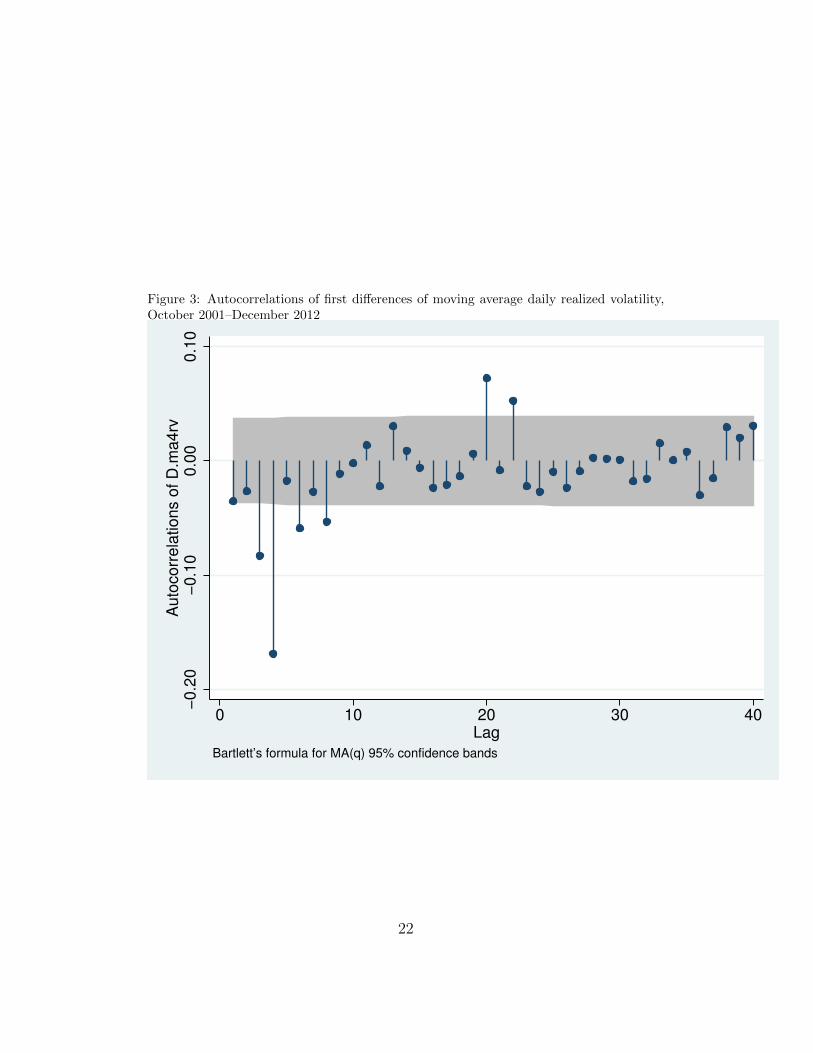
Figure 3: Autocorrelations of first differences of moving average daily realized volatility,October 2001–December 2012

−0

.20

−0

.10

0.0

00

.10

Au

toco

rre

latio

ns o

f D

.ma

4rv

0 10 20 30 40Lag

Bartlett’s formula for MA(q) 95% confidence bands

22

Figure 4: Root mean squared error (RMSE) of volatility forecasts from SV, SVJ models,annual averages 2002–2012

20

40

60

80

100

Ave

rag

e f

utu

res p

rice

.02

.04

.06

.08

.1

2002 2003 2004 2005 2006 2007 2008 2009 2010 2011 2012Year

RMS error, SV RMS error, SVJ

Average futures price

23

Figure 5: Mean absolute error (MAE) of volatility forecasts from SJ, SVJ models, annualaverages 2002–2012

20

40

60

80

100

Ave

rag

e f

utu

res p

rice

.02

.03

.04

.05

2002 2003 2004 2005 2006 2007 2008 2009 2010 2011 2012Year

Mean abs error, SV Mean abs error, SVJ

Average futures price

24

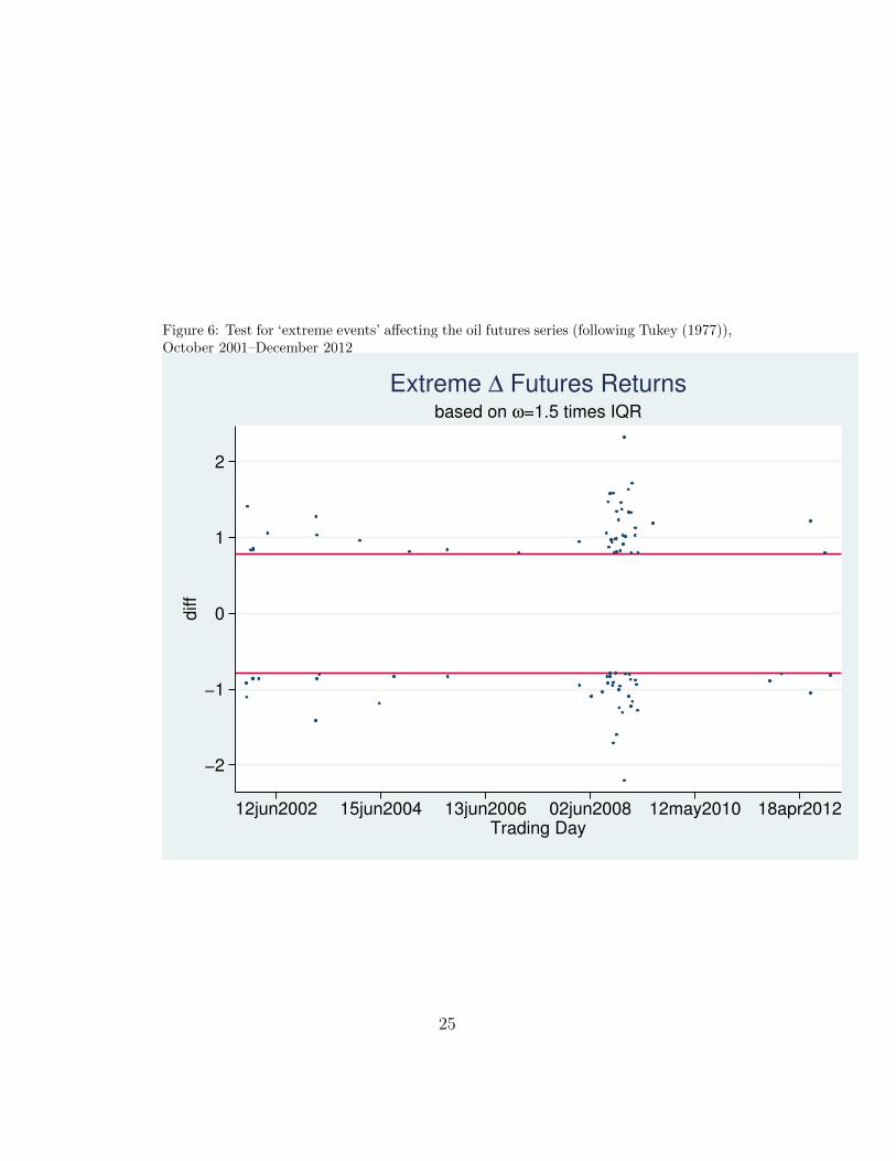
Figure 6: Test for ‘extreme events’ affecting the oil futures series (following Tukey (1977)),October 2001–December 2012

−2

−1

0

1

2

diff

12jun2002 15jun2004 13jun2006 02jun2008 12may2010 18apr2012Trading Day

based on ω=1.5 times IQR

Extreme ∆ Futures Returns

25