July 30, 2018 - barrett.dyson.cornell.edubarrett.dyson.cornell.edu/NEUDC/paper_304.pdf · The loan was offered by Amendis, the local water provider, as part of a program that sought

The Hidden Role of Piped Water in the Prevention of Obesity. Experimental and

Non-Experimental Evidence from Developing Countries

Patricia I. Ritter∗

July 30, 2018

Abstract

Child obesity in developing countries is growing at an alarming pace.This study investigates whether expanding access to piped water athome can contribute to stopping this epidemic. It exploits experimen-tal data from Morocco and longitudinal data from the Philippines andfinds that access to piped water at home reduces childhood BMI andobesity rates. This study further shows that the effect is generated by areduction in the consumption of soft drinks and food prepared outsidethe home. Finally, the study shows that the effect of access to piped wa-ter on healthy nutritional status can be hidden, if access of piped waterat home reduces diarrhea prevalence, since this in turn increases BMI.

1 Introduction

As of 2010, there were 43 millions children worldwide age 5 or younger overweightor obese. Of these, 35 millions live in developing countries (Harvard, 2018). In Mo-rocco, the overweight rate for children under five years of age is one of the highest

∗Department of Economics, University of Connecticut. 365 Fairfield Way, Unit 1063. Storrs, CT06269-1063. E-mail: [email protected]. I am grateful to Dan Black, Kerwin Charles, DavidMeltzer and Ioana Marinescu for their valuable comments and suggestions.

1

in the world, surpassing the US and Mexico. Obesity can seriously deteriorate chil-dren heart, lungs, muscles and bones, kidneys and digestive tract, and hormonesthat control blood sugar and puberty. It increases the likelihood of adult obesity ,and with that increases the risk of cardiovascular diseases and of unemployment.This study investigates whether access to drinking water can contribute to the fightagainst the obesity epidemic in developing countries. Numerous studies have shownthe benefits of access to drinking water on waterborne diseases (Galiani, Gertler andSchargrodsky, 2005; Gamper-Rabindran, Khan and Timmins, 2010), but to the bestof my knowledge, no study has investigated whether access to piped water at homereduces body weight and obesity rates.

Since lack of piped water at home increases the cost of drinking water, it mightinduce people to substitute toward soft drinks, or other liquids high in calories.Likewise, lack of piped water at home increases the cost of cooking and of washingdishes, thus, it might induce people to substitute toward eating food outside thehome including snacks, fast food and street vendors’ food that typically have morecalories than home-made food. The two implicit conditions for this to happen is,first, that families that do not have piped water at home do have enough moneyand do have access to soft drinks, snacks, fast food or street-vendors food. This, ofcourse, is not the case in many rural areas and among extremely poor individuals indeveloping countries. However, lack of access to piped water at home is far frombeing a problem exclusively from extremely poor individuals and from rural areas;one in every three urban dwellers in developing countries does not have piped waterat home (UnitedNations, 2015). Meanwhile, western food companies are targetingdeveloping countries as the richest nations are shrinking their demand (Jacobs andRichtel, 2017; Euromonitor-International, 2010; Deogun, 1999).

The second condition is that food outside the home, especially high-calorie foodlike soft drinks, snacks, street vendors food and fast-food, is a substitute of waterand home-made food. This condition does not necessarily hold; families might de-mand only closer substitutes like bottled water or water from private trucks, andcommunal “home-made” food, for example. In this regard, there is evidence that atleast water and soft drinks are substitutes, moreover, that contaminated water andsoft drinks are substitutes; Ritter (2018) finds that households without piped water

2

at home were especially responsive to a drastic decrease in the price of soda in Peru,increasing their consumption of soda and their obesity rates, while reducing diar-rhea prevalence, suggesting that they reduced their consumption of contaminatedwater.

In principle, therefore, it is plausible that if families get access to piped water athome they will reduce their consumption of food outside the home, and this mightreduce their obesity rates. Empirically, however, it is not easy to test this claim.First, access to piped water at home is typically not random; individuals with ahigher income are more likely to have water at home and are also more likely todrink soft drinks and eat fast-food (while in developed countries they might be infe-rior goods, in developing countries these types of food are typically normal goods),people who have access to piped water at home also typically live in more urban-ized areas with more access to stores, street vendors and markets. Second, accessto clean water at home might reduce the consumption of food outside the home butit might also reduce diarrhea prevalence, and a reduction in diarrhea prevalence hasthe opposite effect on BMI (Kremer et al., 2011). Thus, BMI should decrease withthe reduction in the consumption from eating outside the home, but increase withthe reduction in diarrhea. If the effect on diarrhea is strong enough, it can hide theimportant benefits of drinking water access for maintaining a heathy weight; afterall, having a normal BMI (greater than 18 and smaller than 25) by offsetting theeffect of consuming high-calorie snacks and street food with chronic diarrhea is notas healthy as having a normal BMI by consuming home-made food.

This study examines the effect of access to piped water at home on BMI and obesityrates, exploiting both experimental and non-experimental data. The experimentaldata comes from a social experiment carried out by Devoto et al. (2012) in the cityof Tangiers, Morocco. None of the households that took part in the experiment hadpiped water at home in the baseline but all of them had access to a nearby public tapwith clean water. Connection to piped water at home improved the quantity of waterconsumed but not the quality, and therefore had no effect on diarrhea prevalence De-voto et al. (2012). This context is ideal for the analysis of the present paper, becauseit allows me to isolate the effect on BMI through the potential effect on consump-tion of food outside the home, without the potential offsetting effect of diarrhea

3

on BMI. This estimation is relevant not only as an empirical exercise, but also forpublic policy recommendations; there have been great advances in improved watersources worldwide but access to piped water at home is still very limited (Duflo,Galiani and Mobarak, 2012). Moreover, some studies suggest it is not clear that issocially profitable (Fewtrell et al., 2005; Devoto et al., 2012; Bennett, 2012), thesecost and benefit analyses, however, do not include the potential effect of access topiped water at home on obesity rates.

The non-experimental data comes from the Cebu Longitudinal Health and Nutri-tion Survey, a cohort of Filipino women and their children from the MetropolitanCebu area. The childhood obesity in this area is very low, as opposed to the cityof Tangiers. Thus, the present study uses this data to apply an “acid” test of theexternal validity of the experiment in Morocco. Additionally, this data has dailydiet information, allowing me to investigate potential channels.

Results from the experiment show that access to piped water at home decreasedBMI and obesity rates among children age 0 to 5 in the city of Tangiers, Morocco.Results from the longitudinal analysis, in a very different context with zero child-hood obesity in (Cebu, Philippines), also show that access to piped water at homedecreased BMI among children age 10 to 19. Furthermore, results from this analy-sis confirm the hypothesis that access to piped water at home reduces consumptionof of soft drinks and food outside the home, and that the effect of access to pipedwater on BMI through diarrhea is positive and large enough to “hide” the effect ofaccess to piped water on BMI through the reduction in consumption.

Obesity, in particular childhood obesity is increasing at an alarming pace. Very fewinterventions have thus far proven to be effective in the fight against this epidemic(Cawley, 2015). This study shows that access to piped water at home has additionalsocial benefits and that it can play an important role in the fight against obesity.

4

2 Experimental Evidence

2.1 Setting and Experimental Design

This study exploits an experiment carried out by Devoto et al. (2012) in the cityof Tangiers, north urban area of Morocco. The original purpose of the experimentwas to estimate the effect of households’ connection to the drinking water networkon several well-being indicators including water-borne diseases, time use, socialintegration and mental well-being. The intervention consisted of information aboutand assistance with the application for a loan to finance the connection to the waternetwork. The loan was offered by Amendis, the local water provider, as part of aprogram that sought to increase access to the water and sanitation network. Theconnection to the water network was at full cost, but the loan was interest-free. Thetreatment encouraged take-up of the loan by providing information and a marketingcampaign, pre-approving the loan and offering the collection of the down-paymentat home, saving them the trip to the branch office.

Devoto et al. (2012) selected a sample of 845 households from three zones of thecity of Tangiers. The households selected had no water connection at home buthad a public tap in their neighborhoods. The randomization was done at a “cluster”level, where a cluster was defined as two adjacent plots or two plots facing eachother on the street or up to one house apart. It was stratified by location, watersource, the number of children under five, and the number of households within thecluster. Data was collected before the intervention in August 2007 (hereafter “Base-line”), and 5 months after the water connection (6 months after the intervention), inAugust 2008 (hereafter “Endline”).

2.2 Summary Statistics and Balance Check

The sample of the original experiment consists of 315 clusters and 434 householdsin the treatment group and 311 clusters and 411 households in the control group.

5

This study works with a subsample, since anthropometric indicators were takenonly from children ages 0 to 7 (in the Endline). The resulting number of observationin the Endline is 347, corresponding to 126 clusters and 146 households in thetreatment group and 105 clusters and 115 households in the control group.

BMI is calculated by the ratio of weight in kilograms divided by the square ofheight in meters. Definitions of anthropometric indicators follow the World HealthOrganization (WHO) 2006 standards. BMI-for-age is age- and sex-specific and rep-resents the (standardized and adjusted) deviation of a child’s BMI from the medianvalue of a reference population selected by WHO. Overweight and obese childrenare defined as those with BMI-for-age greater than one and two standard deviations,respectively. Underweight children are those with BMI-for-age lower than negativetwo standard deviations.

Table 1 shows the balance check in the baseline from this subsample. One inconve-nient of the data is that the number of children with anthropometric indicators in theBaseline is less than half of that in the Endline, and the number is in fact too smallto detect significant differences. Fortunately, the most important outcome variable,obesity rate, is actually higher for the treatment group then for the control group.

In terms of household variables, we do have the same number of observations in thebaseline and endline. We can see only two significant differences between treatmentand control group. One is in the number of children age 15 or less. We can seehowever, that the difference in the Endline of the number of children age 7 or less(that is our sample of interest) is not significantly different. The second differenceis in an assets indicator. This indicator was constructing following Devoto et al.(2012)’s strategy, and should reflect differences in wealth or income. However, inDevoto et al. (2012)’s sample there is no difference in this indicator, and in oursample, there is no significant difference in any other income or wealth indicator.

It is important to notice that by sample design no household in either group hadaccess to piped water at home but all households have access to piped water froma public tab. The average distance to water is 142 meters. This distance might notseem too large, but just not having the water in the convenience of home mightmake a lot of difference.

6

Morocco has one of the highest rates of childhood obesity in the world according tothe WHO. This sample is not the exemption: between 16% and 18% of the childrenage 0 to 5 were obese in the baseline. It is important to note, that weight was takentwo times, and I work with the average weight in order to calculate the BMI andBMI-for-age. Moreover, I eliminate observations with the BMI from the percentile99 and 1 in order to eliminate impossible values. Nevertheless, my sample’s averageis much less precise than those of the reference population; instead of a standarddeviation of one, this sample has a standard deviation of circa 2.

2.3 Empirical Strategy

This section estimates intent-to-treat effects (ITT) and local average treatment ef-fects (LATE). The ITT estimator captures the effect of being selected for treatment(but not necessarily treated). This effect is estimated from the following specifica-tion:

Yi, j = βo +β1Tj +β2Xi, j + εi, j

where Yi, j stands for BMI or other outcome for child i in cluster j, Tj stands forwhether the cluster j was selected to the treatment, Xi, j stands for baseline charac-teristics children i in cluster j, and εi, j stands for the error term. Baseline charac-teristics include: a dummy that indicate whether the household was connected bya hose to the neighbor’s or a public tap, an assets indicator, the number of adultswith a paid job and whether or not the water they had access to before the treatmenttasted good.

The LATE estimator captures the effects of actually having received the treatment,using the selection to the treatment as an instrumental variable. The first stageestimates the effect of being selected for the treatment on the probability of beingconnected to the water network from the following specification:

7

Ci, j = β2 +β3Tj +β4Xi, j + εi, j

where Ci,t stands for whether the child lives in a house connected to the water net-work.

The second stage estimates the effect of being connected to the water network onsome outcome from the following specification:

Yi, j = βo +β1Ci, j +β2Xi, j + εi, j

where Ci, j stands for the predicted probability of being connected to the water net-work estimated in the first stage.

All the regressions have standard errors clustered at the cluster level. Under the as-sumption of constant treatment effect, β1 could be interpreted as the average treat-ment effect. In the absence of such assumption, this estimator should be interpretedas the effect of access to the water network on weight outcomes of children of the“complier” households. That is, households that were encouraged by the interven-tion to connect to the water network but would not have done so in the absence ofthe intervention.

2.4 Results Experimental Evidence

As explained above this intervention relied on an encouragement design as opposedto a direct intervention. Hence, the first question we need to assess is whether theintervention increased water connection significantly. Table 2 shows that, in fact,the intervention successfully encouraged water connections; 80% of the treatmentgroup got connected to the water network, while only 19% of the control group did.Column 2 shows that this estimation changes little with the inclusion of controlvariables.

8

Table 3 presents the effect of the treatment on BMI-for-age. The first and thirdcolumn show the estimated ITT without and with controls, respectively. Accordingto our preferred estimate (column 2), 6 months after the intervention children ofthe treatment group have average BMI-for-age lower than children of the controlgroup by 0.35 units or 0.18 standard deviations. Column 2 and 4 show the LATEestimates without and with controls, respectively. As expected, these estimates arelarger in magnitude but not significant.

Table 3 also presents the effect of the treatment on obesity rates. The first columnshows that 6 months after the intervention, 23% of the children of the control groupare obese, while only 12% of the children of the treatment group are obese, andthis difference is statistically significant. According to the LATE estimator, theeffect of being connected to the water network reduced the probability of beingobese by almost 10 percentage points. As we know, these estimates capture theeffect of access to the water network on the likelihood of being obese of childrenof the “complier” households. Since the intervention consisted in information andassistance with the loan, but no difference in the loan conditions, those in the pool ofhouseholds who connected to the network as a consequence of the intervention maynot have been very educated but had enough money to repay the loan. Note that thispool of households might have particularly large effects, insofar as low-educatedhouseholds are less aware of the detrimental consequences of childhood obesity,and households with enough money to repay the loan can also probably afford tobuy high-caloric beverages instead of walking to the nearest public tap to drink freewater. Thus, my estimated Local Treatment Effect (LATE) might be significantlyhigher than the average treatment effect of connecting to water network. Still, theeffects are so large that, even if the average effect is considerably smaller, it mightstill be economically and statistically different from zero.

Table 3 shows the effect of the treatment on the BMI and obesity rates calculatedwith the averages of the two measures there are in the data. It is important tomention, however, that the estimations on the two BMI measures, separately, arealmost identical from each others (results from these regression are available uponrequest). Still, it is possible that the results in BMI and obesity rates are spuriouslygenerated by the small number of observations. Therefore, as a mean to increase

9

the reliability of the results, I test the following hypothesis; if my results reflect theeffect of the program, the effect should be smaller for households that before theprogram were connected to the public tap either through a hose or an informal pipe,since they already had running water at home. On the contrary, if the true effect ofthe program would be zero, it shouldn’t be any different for people that before theprogram were connected to the public tap either through a hose or an informal pipe.Table 4 shows the estimation results. We can see that the effects of the program onBMI and obesity rates come mostly from households that before the program werenot connected to the public tap.

3 Non-Experimental Evidence

3.1 Data and Summary Statistics

This section exploits data from the Children of the Cebu Longitudinal Health andNutrition Survey. This study follows a cohort of Filipino women and their childrenfrom the Metropolitan Cebu area who were born between May 1, 1983, and April30, 1984 . After the baseline, they surveyed children’s anthropometric indicatorsand diet diaries in 1991, 1994, 1998, 2002, 2005. However, I only work with datauntil 2002, since the WHO standards that are used to calculate the BMI-for-ageare comparable only up to age 19 and there are no children age 19 or younger inyear 2005. Additionally, information about whether children had piped water athome, our main explanatory variable, was collected only since 1991,1 and since Iuse lagged variables to estimate the effect on BMI, I am not able to estimate theeffect on BMI for year 1991. Finally, the first round of food diaries in 1991 differsfrom the following diaries, which means I am also not able to use the food diariesfrom 1991. I restrict the sample to the urban barangays, which represent 73% of thesample. Nevertheless, the results remain significantly similar when I work with thecomplete sample.

1Explain how they collected water in the baseline

10

Table 5 shows the summary statistics of my sample. Children are 15 years old andweight 40 kilos on average. The overweight rate is only 4% and there are no obesechildren. This represents a very different context from Tangiers. However, this isunsurprising given that even with respect to the urban population/areas from Cebu,only around half of the sample lives within walking distance of a store. Only 12%has access to piped water at home and 36% has access to piped water either insideor outside the house. Walking time to a source of water is 2.4 minutes on average.41% of women fetched water and spent 40 minutes doing so in the week previous tothe baseline. Women at that time, however, were pregnant, so these numbers mightbe underestimating the real percentage and time of women fetching water regularly.

Table 5 also shows, as we would expect, that children with piped water at homehave mothers with higher incomes, live in more populated areas, eat more foodoutside the home, drink more sodas and are more likely to be overweight.

3.2 Model and Empirical Strategy

This section exploits the longitudinal feature of the data to apply a Fixed EffectModel at the individual level. The effect on food consumption is estimated fromthe following specification:

Yi,t = βo +β1Wateri,t +β2Xi,+αi +φt + εi,t

where Yi,t stands for the consumption of food outside the home or other type ofconsumption of child i in year t, Wateri,t stands for whether the child i had pipedwater at home in year t, Xi,t stands for control variables of child i inyear t, αi and φt

stand for child and year fixed effect, respectively, and εi,t stands for the error term.Control variables include: mother’s income and fixed effects of the barangay wherethe child currently lives. The same child can live in several barangays across rounds,because this survey follows the children and their families even if they move.

The effect on standardized BMI-for-age and overweight rate is estimated from thefollowing specification:

11

Yi,t = βo +β1Wateri,t−1 +β2Wateri,t−1Diarrheai,s +β3Xi,t−1 +αi +φt + εi,t

In this case, I use lagged variables. According to Hall et al. (2011), the total effectof a change in calories on weight takes a little bit more than 3 years. Rounds inthis survey happen every 3-4 years, thus by using lagged explanatory variables,the estimated effect correspond to the long-term effect of access to piped water onBMI. We also know that access to water can reduce diarrhea prevalence and thisin turn can increase BMI. Unfortunately, there is no data on diarrhea prevalence inall rounds. Thus, in order to control, at least imperfectly, for this off-setting effect,this specification controls for the interaction of access to piped water at home andwhether the child’s mother experienced at least one episode of diarrhea in the 3months preceding the baseline, s. I do not use whether the child had diarrhea in thebaseline, because as babies most were breastfed and diarrhea among babies is verycommon even with access to clean water. Thus, β1 now should capture the effectaccess to piped water on children, who were exposed to no or little contaminatedwater; that is the effect on BMI due only to a reduction in the consumption offood outside the home and soft drinks, while β2 should capture the differentialeffect of access to piped water on children that were exposed to contaminated water;that is, the additional and off-setting effect on BMI through reduction in diarrheaprevalence. If my predictions are correct, β1 should be negative and β2 should bepositive.

3.3 Results

Table 6 shows the results on food eaten outside the home, soft drinks, home-madefood, and milk. The simple correlation between piped water at home and quantityof food eaten outside the house is positive due to several third factors that are posi-tively correlated with both variables. The first obvious group of variables are thoserelated to time-invariant characteristics of the children, such as wealth, parents’ ed-ucation, and knowledge about nutrition. The first column shows the results froma FE model without any additional control variable. As we can see, controlling

12

for time-invariable characteristics of the children eliminates the apparent positiveeffect on food eaten outside the house. A second important third factor correlatedwith both variables is time. In the last decades there has been an increase in theconsumption of food outside the house in many developing countries, in particu-lar in the consumption of snacks and fast food, both for families/individuals withand without piped water at home. Simultaneously, there has been an increase inthe number of households with access to piped water at home. In order to con-trol for these simultaneous increases, column 2 includes year fixed effects, and aswe would expect, our coefficient of interest grows in absolute terms and becomesstatistically significant. Column 3 controls for income. Naturally, income is pos-itively correlated with having access to piped water and with eating food outsidethe house, thus controlling for income increases the magnitude and the significanceof our estimated coefficient. Finally, areas with greater access to piped water havetypically better access to food outside the home. If individuals move to these areas,we will see an increase in the likelihood of access to both of these things. This dataset follow individuals that move; for this reason, column four include fixed effectsof the barangay, where they currently live. Again we observe an increase in themagnitude of the estimate. According to our last and preferred estimate, access topiped water at home decreases the consumption of food outside the home by ap-proximately 48 grams per day, which represents a decrease of 15%. A very similarpattern can be observed in the estimation of the effect of piped water at home onsoda consumption. According to our last and preferred estimate, access to pipedwater at home decreases the consumption of soda by approximately 20 millilitersper month, which represents an increase of 29%.

Table 6 also shows the effect on home-made food and milk. Here we see that ac-cess to piped water at home has no significant effect on these consumptions. Theseresults are reassuring in several ways. First of all, it enables us to discard the al-ternative hypothesis that access to piped water at home might be correlated with adecrease in income or another omitted variable that decreases all types of consump-tion. Second, our story predicts that access to piped water at home should generatea decrease in soft drinks because it generates an increase in the consumption of wa-ter, not on milk. An alternative story might be that decrease in soft drinks happens

13

because of an increase in the consumption of milk that is spuriously correlated toaccess to piped water. Hence, it is reassuring that I find no effect on the consump-tion of milk. Finally, it is important to note a couple of things related to effect inconsumption of home-made food. First of all, although the effect on the quantity ingrams of home-made food is not statistically significant, the effect on the percentageof home-made food that children consume is positive and statistically significant, aswe can see in Table 7. According to our last and preferred estimate, access to pipedwater at home increases the consumption of home-made food by approximately 4%points or 5%.Second, while the effect on consumption of home-made food, is pos-itive it is not as large in magnitude as the decrease in food outside the home. Thusaccess to piped water at home generated a substitution away from food outside thehome toward home food but this substitution does not seem to be completely offset(although this difference is not statistically significant). Thus, there should be aneffect on weight resulting from a change on the quality of food, but probably alsoon the quantity of food. Table 9 of the appendix shows very similar estimates whenrural areas are included in the sample.

Table 8 shows the results on standardized BMI-for-age and overweight rate (resultson obesity rates are omitted, given that rates are close to 0 for this population).The first column shows the effect of a simple fixed effect strategy, and we can seethat the difference in BMI within children with and without piped water at homeis smaller in magnitude than the cross-child difference, but it is still positive. Thesecond column includes additionally year fixed effects. We can see that includingthese fixed effects eliminates the significance of the positive correlation betweenaccess to piped water at home and BMI. Column 3 includes the interaction of pipedwater at home and instances in which the child’s mother experienced diarrhea inthe baseline. We can see that the effect of access to piped water at home on BMI inthe absence of diarrhea is negative and the additional effect of access to piped waterthrough diarrhea on BMI-for-age is positive. Column 4 controls additionally forincome, and the effect of piped water on BMI becomes statistically significant. Fi-nally, column 5 includes fixed effects of the barangay, where the children currentlylive, and we again observe an increase in the magnitude of the estimate. Accordingto our last and preferred estimate, access to piped water at home reduces BMI-for-

14

age by around 0.23 standard deviations but increases BMI-for-age by around 0.31standard deviation through its reduction on diarrhea prevalence. Table 8 also showsthat the same pattern for the estimations of the effect of access to piped water athome on child overweight rate. However, none of the estimations are statisticallysignificant. Finally, table 10 of the appendix shows very similar estimates whenrural areas are included in the sample.

4 Conclusions

This study investigates whether expanded access to piped water at home can con-tribute to the fight against obesity in developing countries. It exploits experimentaldata from the city of Tangiers, Morocco and longitudinal data from the city ofCebu, the Philippines. Results from the experiment show that access to piped wa-ter at home decreased BMI and obesity rates among children age 0 to 5 in the cityof Tangiers, Morocco. Results from the longitudinal analysis, in a very differentcontext with zero childhood obesity, also show that access to piped water at homedecreased BMI among children age 10 to 19 in Cebu, Philippines. Furthermore,results from this analysis confirm the hypothesis that access to piped water at homereduces consumption of soft drinks and food outside the home, and that the effectof access to piped water on BMI through diarrhea is positive and large enough to“hide” the effect of access to piped water on BMI through the reduction in con-sumption.

This study suggests that access to piped water at home might play an importantrole in the fight against obesity in developing countries. It also provides evidencethat programs that facilitate water access at home in urban areas can have importanthealth benefits, even in the absence of effects on diarrheal diseases. This result is es-pecially relevant given that, while there have been great advances in improved watersources worldwide, access to piped water at home is still very limited. Finally, thispaper contributes to a better understanding of the demand and willingness to payfor piped water at home: the substitution away from food outside the home towardhome-made food might generate some monetary savings. Additionally, individualswould likely welcome losing a few extra pounds.

15

ReferencesBennett, Daniel. 2012. “Does clean water make you dirty? Water supply and sani-

tation in the Philippines.” Journal of Human Resources, 47(1): 146–173.

Cawley, John. 2015. “An economy of scales: A selective review of obesity’seconomic causes, consequences, and solutions.” Journal of health economics,43: 244–268.

Deogun, Nikhil. 1999. “Aggressive push abroad dilutes Coke’s strength as big mar-kets stumble.” The Wall Street Journal.

Devoto, Florencia, Esther Duflo, Pascaline Dupas, William Parienté, and Vin-cent Pons. 2012. “Happiness on Tap: Piped Water Adoption in Urban Morocco.”American Economic Journal: Economic Policy, 68–99.

Duflo, Esther, Sebastian Galiani, and Mushfiq Mobarak. 2012. “Improv-ing access to urban services for the poor: open issues and a framework fora future research agenda.” J-PAL Urban Services Review Paper. Cambridge,MA: Abdul Latif Jameel Poverty Action Lab. http://www. povertyactionlab.org/publication/improving-access-urban-services-poor.

Euromonitor-International. 2010. “Who Drinks What: Identifying InternationalDrinks Consumption Trends.”

Fewtrell, Lorna, Rachel B Kaufmann, David Kay, Wayne Enanoria, LaurenceHaller, and John M Colford. 2005. “Water, sanitation, and hygiene interven-tions to reduce diarrhoea in less developed countries: a systematic review andmeta-analysis.” The Lancet infectious diseases, 5(1): 42–52.

Galiani, Sebastian, Paul Gertler, and Ernesto Schargrodsky. 2005. “Water forlife: The impact of the privatization of water services on child mortality.” Journalof political economy, 113(1): 83–120.

Gamper-Rabindran, Shanti, Shakeeb Khan, and Christopher Timmins. 2010.“The impact of piped water provision on infant mortality in Brazil: A quantilepanel data approach.” Journal of Development Economics, 92(2): 188–200.

Hall, Kevin D, Gary Sacks, Dhruva Chandramohan, Carson C Chow, Y ClaireWang, Steven L Gortmaker, and Boyd A Swinburn. 2011. “Quantification ofthe effect of energy imbalance on bodyweight.” The Lancet, 378(9793): 826–837.

Harvard. 2018. “Child Obesity. Too Many Kids Are Too Heavy, Too Young.” Har-vard. T.H. Chan School of Public Health.

16

Jacobs, Andrew, and Matt Richtel. 2017. “How Big Business Got Brazil Hookedon Junk Food.” New York Times.

Kremer, Michael, Jessica Leino, Edward Miguel, and Alix Peterson Zwane.2011. “Spring cleaning: Rural water impacts, valuation, and property rights in-stitutions.” The Quarterly Journal of Economics, 126(1): 145–205.

Ritter, Patricia I. 2018. “Soda Consumption in the Tropics: The Trade-Off be-tween Obesity and Diarrhea in Developing Countries.” Working Paper.

UnitedNations. 2015. “Water and Cities.” Web Page.

17

Table 1: Balance Check - Experimental

Obs. Treatment Control r1Age 160 2.7 3.0 0.21Female 160 53% 59% 0.43Weight 160 13.7 14.3 0.34Height 160 90.3 92.2 0.40BMI 160 16.7 16.9 0.61BMI-for-age 160 0.9 1.0 0.63Underweight 160 1% 0% 0.37Overweight 160 37% 41% 0.63Obesity 160 26% 18% 0.26ExtremeObesity 160 12% 11% 0.83

Num.members 350 5.7 5.9 0.41Num.children<=15 350 2.4 2.8 0.01Num.children<=7 350 1.8 1.9 0.19Headmale 350 0.9 0.9 0.31Headage 350 40.9 40.3 0.65Headmarried 350 0.9 0.9 0.73Headnoeducation 350 0.3 32% 0.42Headprimaryeducation 350 0.5 43% 0.14

Assetsscore 348 0.0 0.4 0.04Headincome 350 1,177 1,156 0.86Familyincome 318 4.5 4.7 0.32Num.roomsperperson 346 0.7 0.6 0.24

Pipedwaterathome 348 0% 0% 1.00Pipedwateranywhere 348 100% 100% 1.00Chlorinewater 103 0.7 0.6 0.39Wateruseinthelast7days 332 0.4 0.5 0.91Distancetowater(mts) 348 153.0 136.5 0.29Connectiontoneighbors 348 0.2 0.2 0.85

18

Table 2: First Stage Results - Experimental Data

First Stage First Stagecoef/se coef/se

Assigned to Treatment Group 0.606*** 0.610***(0.057) (0.057)

Controls X

_cons 0.192*** 0.070***(0.041) (0.041)

Number of observations 349 349R2 0.364 0.364note: .01 - ***; .05 - **; .1 - *;

19

Table 3: Results on BMI-for-Age and Obesity Rates - Experimental Data

ITT IV ITTc IVccoef/se coef/se coef/se coef/se

Assigned to Treatment Group

-0.265 -0.348*

(0.237) (0.211)Household got connected

-0.437 -0.578

(0.390) (0.353)

Control Variables X X

_cons 1.036*** 1.120*** 6.536*** 6.477***(0.192) (0.255) (1.017) (1.042)

Number of observations 349 349 348 348R2 0.005 0.005 0.221 0.210note: .01 - ***; .05 - **; .1 - *;



-0.091** -0.107**


-0.150** -0.177**

(0.076) (0.072)


_cons 0.231*** 0.260*** 1.205*** 1.187***(0.037) (0.050) (0.164) (0.178)

Number of observations 349 349 348 348R2 0.014 . 0.178 0.129note: .01 - ***; .05 - **; .1 - *;

Obesity

BMI

20

Table 4: Robustness Results on BMI-for-Age and Obesity Rates - ExperimentalData



-0.425* -0.526**

(0.254) (0.232)

Household got connected

-0.711* -0.871**

(0.426) (0.401)Treatmentxpublictap 1.054 1.091**

(0.655) (0.550)Connectedxpublictap 1.701 1.775**

(1.092) (0.896)





-0.104** -0.122***


-0.173** -0.205***

(0.080) (0.078)Treatmentxpublictap 0.089 0.095

(0.126) (0.108)Connectedxpublictap 0.150 0.168

(0.200) (0.172)



BMI

Obesity

21

Table 5: Summary Statistics - Longitudinal Data

With WithoutObs. Mean Mean Mean

Age (in years) 4,012 14.93 15.29 14.83(2.97) (2.97) (2.96)

Male (%) 4,012 0.52 0.54 0.52(0.50) (0.50) (0.50)

Height (in cm) 3,977 147.39 150.29 146.55(12.79) (11.85) (12.94)

Weight (in kg) 3,998 39.93 42.36 39.22(11.09) (10.91) (11.04)

Standardized BMI for age 4,012 -0.88 -0.78 -0.91(1.00) (1.05) (0.98)

Overweight (%) 4,012 0.04 0.05 0.04(0.20) (0.21) (0.19)

Obesity (%) 4,012 0.00 0.00 0.00(0.00) (0.00) (0.00)

Underweight (%) 4,012 0.13 0.12 0.13(0.34) (0.33) (0.34)

Piped water at home (%) 4,012 0.23 1.00 0.00(0.42) (0.00) (0.00)

Piped water anywhere (%) 4,012 0.49 1.00 0.34(0.50) (0.00) (0.47)

Mother fetched water 1st. Round (%) 4,000 0.41 0.28 0.45(0.49) (0.45) (0.50)

Min. p/week m. fetched water 1st. Round 4,000 40.43 27.64 44.15(59.16) (47.62) (61.62)

Walking time to store (in minutes) 1,859 7.66 7.51 7.71(7.45) (6.32) (7.81)

Mother's income 3,679 206.45 474.83 128.87(3,972) (8,349) (423)

Density (n. of houses within 50 mts) 4,012 19.14 19.54 19.02(2.99) (2.07) (3.20)

Food outside the home (grs/day) 3,993 317.51 374.58 300.97(277) (299) (267)

Home-made food (grs/day) 3,984 633.54 635.68 632.91(335) (336) (334)

Soft drinks (mls/day) 3,988 70.79 95.13 63.71(131) (150) (125)

Milk (mls/day) 3,972 3.49 4.88 3.09(11.32) (13.80) (10.47)

Piped Water at HomeTotal

22

Table 6: Results on Consumption - Longitudinal Data

(1) (2) (3) (4) (1) (2) (3) (4)coef/se coef/se coef/se coef/se coef/se coef/se coef/se coef/se

HH has piped water inside home or yard

-0.76 -32.73* -39.38** -47.59** 12.82 -10.81 -16.94* -20.37**

(18.41) (18.83) (19.65) (20.75) (9.50) (9.26) (9.49) (9.90)

Individual FE X X X X X X X XYear FE X X X X X XIncome X X X XBarangay FE X X

Observations 4,375 4,375 4,019 4,019 4,370 4,370 4,015 4,015R2 0.00 0.06 0.06 0.09 0.00 0.14 0.14 0.16note: *** p<0.01, ** p<0.05, * p<0.1



46.62** -7.89 3.16 10.15 1.57* 1.26 1.00 0.68

(21.73) (20.30) (21.63) (22.49) (0.91) (0.94) (1.00) (0.93)



Home-made food (grs/day) Milk (mls/day)

Food outside the home (grs/day) Soft drinks (mls/day)

23

Table 7: Results on Consumption - Longitudinal Data



0.02 0.02 0.03* 0.04** 52.29* -35.44 -35.31 -38.26

(0.014) (0.014) (0.015) (0.016) (27.206) (25.818) (27.240) (28.615)



Home-made food (%) All Food (mls/day)

24

Table 8: Results on Body Mass Index and Overweight Rate- Longitudinal Data

(1) (2) (3) (4) (5)coef/se coef/se coef/se coef/se coef/se

HH has piped water inside home or yard (lagged)

0.139*** 0.041 -0.140 -0.174* -0.234**

(0.045) (0.046) (0.087) (0.100) (0.106)HH has piped water inside home or yard (lagged)

0.217** 0.246** 0.305**

x Diarrhea 1st Round (0.100) (0.113) (0.121)

Individual FE X X X X XYear FE X X X XDiarrhea X X XIncome X XBarangay FE X

Number of observations 4,061 4,061 4,061 3,668 3,654R2 0.004 0.082 0.083 0.084 0.117note: *** p<0.01, ** p<0.05, * p<0.1



0.017 0.015 -0.015 -0.019 -0.024


0.036* 0.046* 0.051*




Overweight Rate

Standardized BMI-for-Age

25

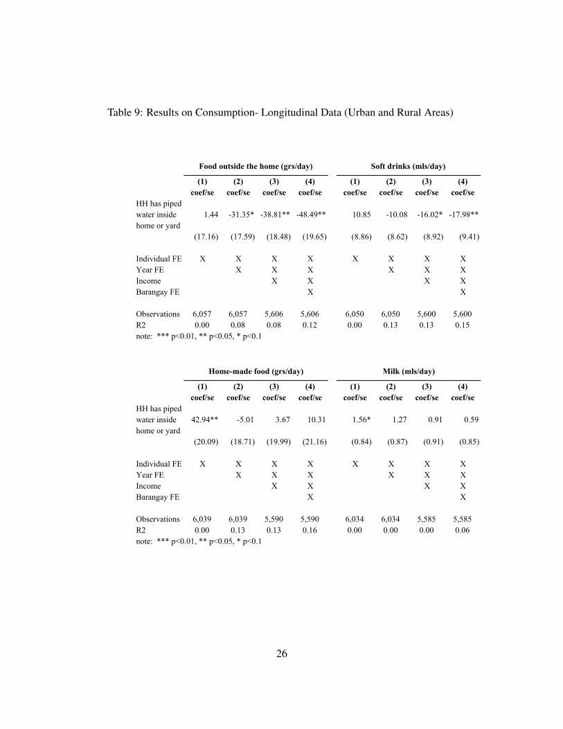
Table 9: Results on Consumption- Longitudinal Data (Urban and Rural Areas)



1.44 -31.35* -38.81** -48.49** 10.85 -10.08 -16.02* -17.98**

(17.16) (17.59) (18.48) (19.65) (8.86) (8.62) (8.92) (9.41)





42.94** -5.01 3.67 10.31 1.56* 1.27 0.91 0.59

(20.09) (18.71) (19.99) (21.16) (0.84) (0.87) (0.91) (0.85)



Food outside the home (grs/day) Soft drinks (mls/day)

Home-made food (grs/day) Milk (mls/day)

26

Table 10: Results on Body Mass Index and Overweight Rate- Longitudinal Data(Urban and Rural Areas)



0.139*** 0.041 -0.136 -0.165* -0.268***


0.210** 0.230** 0.322***






0.014 0.011 -0.026 -0.018 -0.020


0.044** 0.041* 0.046*




Standardized BMI-for-Age

Overweight Rate

27

Documents

July 30, 2018 - barrett.dyson.cornell.edubarrett.dyson.cornell.edu/NEUDC/paper_304.pdf · The loan was offered by Amendis, the local water provider, as part of a program that sought