July 25, 2008 11:25 WSPC/103-M3AS 00302 …lchayes/lchayes_website_folder/new...July 25, 2008 11:25 WSPC/103-M3AS 00302 Mathematical Models and Methods in Applied Sciences Vol. 18,

July 25, 2008 11:25 WSPC/103-M3AS 00302

Mathematical Models and Methods in Applied SciencesVol. 18, Suppl. (2008) 1249–1267c© World Scientific Publishing Company

A STATISTICAL MODEL OF CRIMINAL BEHAVIOR

M. B. SHORT∗, M. R. D’ORSOGNA†, V. B. PASOUR∗,G. E. TITA‡, P. J. BRANTINGHAM§,A. L. BERTOZZI∗ and L. B. CHAYES∗

∗Department of Mathematics,University of California — Los Angeles,

Los Angeles, CA 90095, USA

†Department of Mathematics,California State University — Northridge,


‡Department of Criminology,Law & Society, University of California — Irvine,

Irvine, CA 92697, USA

§Department of Anthropology,University of California — Los Angeles,


Received 28 December 2007Revised 1 February 2008

Communicated by N. Bellomo and F. Brezzi

Motivated by empirical observations of spatio-temporal clusters of crime across a widevariety of urban settings, we present a model to study the emergence, dynamics, andsteady-state properties of crime hotspots. We focus on a two-dimensional lattice modelfor residential burglary, where each site is characterized by a dynamic attractivenessvariable, and where each criminal is represented as a random walker. The dynamics ofcriminals and of the attractiveness field are coupled to each other via specific biasing andfeedback mechanisms. Depending on parameter choices, we observe and describe severalregimes of aggregation, including hotspots of high criminal activity. On the basis of the

discrete system, we also derive a continuum model; the two are in good quantitativeagreement for large system sizes. By means of a linear stability analysis we are ableto determine the parameter values that will lead to the creation of stable hotspots. Wediscuss our model and results in the context of established criminological and sociologicalfindings of criminal behavior.

Keywords: Crime models; reaction-diffusion equations; linear stability.

AMS Subject Classification: 35Q80, 70K99

1. Introduction

One unfortunate aspect of modern life is the presence of crime in every major urbanarea. However, while crime itself is ubiquitous, it does not appear to be uniformly

1249

July 25, 2008 11:25 WSPC/103-M3AS 00302

1250 M. B. Short et al.

distributed within space and time. For example, while some neighborhoods tendto be reasonably safe, others appear far more dangerous and display dense clustersof both property and violent crimes.7, 9, 21, 35 Also, temporal correlations betweencrimes are well documented, with victims or their close neighbors often being repeat-edly targeted within short periods of time.1, 25–27 These spatio-temporal aggregatesof criminal occurrences are commonly referred to as crime “hotspots,” and thanksto recent advances in mapping technology it is possible to track their evolution atfine spatial and temporal scales.44 The typical lifetimes and length scales of crimehotspots are observed to vary depending upon the particular geographic, economic,or seasonal conditions present. Also, depending on the specific category of crimein question, hotspots are seen to emerge, diffuse and dissipate in ways suggestiveof a structured, albeit complex, underlying dynamics. Despite this wealth of data,the efforts of law enforcement agencies towards utilizing empirical knowledge ofhotspots as a tool to fight crime have been hampered by uncertainty about thepredictability of such patterns.31, 34

Many theories have been presented within the criminology community to under-stand why hotspots emerge in some locations rather than others, how they evolve,and how their “macroscopic” size and lifetime features are connected to the “micro-scopic” behaviors of offenders, victims, law enforcement agents, and the local geo-graphy. In general, crimes can only occur when a motivated offender encountersa suitable victim or target in the absence of effective security measures. In thiscontext, the structure of the urban environment may play an important role con-straining the movement of offenders and potential targets. For example, featuressuch as traffic volume, vacant or abandoned property, population density, and thedistribution of so-called crime generators impact crime patterns.2, 11, 21, 37, 41, 42

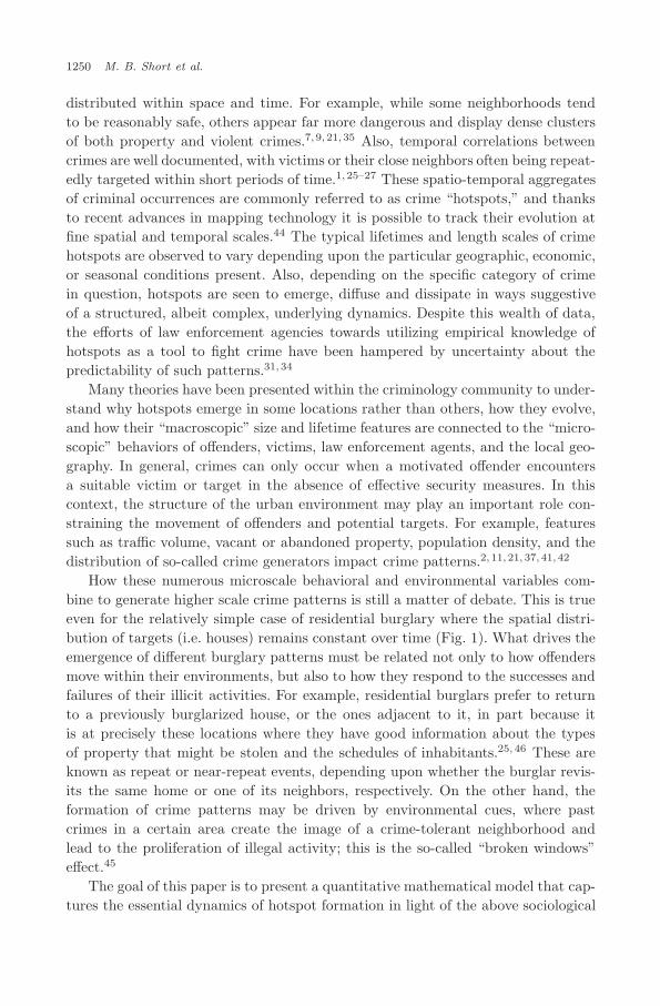
How these numerous microscale behavioral and environmental variables com-bine to generate higher scale crime patterns is still a matter of debate. This is trueeven for the relatively simple case of residential burglary where the spatial distri-bution of targets (i.e. houses) remains constant over time (Fig. 1). What drives theemergence of different burglary patterns must be related not only to how offendersmove within their environments, but also to how they respond to the successes andfailures of their illicit activities. For example, residential burglars prefer to returnto a previously burglarized house, or the ones adjacent to it, in part because itis at precisely these locations where they have good information about the typesof property that might be stolen and the schedules of inhabitants.25, 46 These areknown as repeat or near-repeat events, depending upon whether the burglar revis-its the same home or one of its neighbors, respectively. On the other hand, theformation of crime patterns may be driven by environmental cues, where pastcrimes in a certain area create the image of a crime-tolerant neighborhood andlead to the proliferation of illegal activity; this is the so-called “broken windows”effect.45

The goal of this paper is to present a quantitative mathematical model that cap-tures the essential dynamics of hotspot formation in light of the above sociological

July 25, 2008 11:25 WSPC/103-M3AS 00302

A Statistical Model of Criminal Behavior 1251

Fig. 1. Dynamic changes in residential burglary hotspots for two consecutive three-month periodsbeginning June 2001 in Long Beach, CA. These density maps were created using ArcGIS.

observations. We shall focus on residential burglary, which in many ways is thesimplest crime type, since mobile offenders are coupled to stationary target sites,and further complexity arising from the relative movement between the agents atplay may be ignored.

Our starting point is a discrete lattice system where every site corresponds toa target house. The lattice is further characterized by a series of offender agentsmoving from site to site according to specific rules. As we shall better illustratein Sec. 2, burglar dynamics are strongly coupled to the level of attractiveness oftarget sites, with offender movement and rate of burglary biased towards moredesirable locations. This bias could arise due to the fact that certain homes mayindeed be easier to break into, or that these houses might simply be perceived to bebetter targets. The criminological and sociological effects described earlier will beincorporated into our model by letting the degree of attractiveness of each site be adynamic, non-uniform quantity dependent upon both previous burglary events atthe same location and memory effects from burglaries at neighboring sites. We willbe interested in the role of this feedback loop on the dynamics and morphology ofthe criminal hotspots.

A continuum derivation based upon the discrete model will also be presented.Here, we coarse-grain our discrete grid so that burglars are locally described bya number density function, and interactions with the environment are embodiedvia coupling of this function with the coarse-grained attractiveness. Our continuumcrime model will consist of two coupled reaction-diffusion-like equations describingthe spatio-temporal evolution of number density and attractiveness, giving rise tohotspot formation. In the limit of large criminal populations and lattice sizes, thediscrete and continuum models exhibit similar features.

July 25, 2008 11:25 WSPC/103-M3AS 00302


2. Discrete Model

2.1. Overview

Our discrete burglary model consists of two components — the houses at whichburglaries occur, and the criminal agents that commit these burglaries. The housesare imagined as existing on a two-dimensional lattice; for simplicity, we choose arectangular grid with constant lattice spacing � and periodic boundary conditions,though more complicated arrangements that better reflect the layout of an actualcity are possible. In conjunction with the lattice spacing �, a discrete time unitδt over which criminal actions will occur is also chosen. Each house is describedby its lattice site s = (i, j) and a quantity As(t), which we will refer to as theattractiveness of the site. As the name implies, As(t) is a measure of the burglars’perception of the attractiveness of the home at site s, and we model it as beingequivalent to the statistical rate of burglary at site s when a burglar is present.We make no attempt to derive this attractiveness from underlying properties of theresidence, such as value, security, or location. Instead, we treat the attractivenessin the spirit of collective behavior, modeling it after the sociological phenomena ofrepeat and near-repeat victimization and the broken windows effect discussed inthe introduction. With this in mind, we let

As(t) ≡ A0s + Bs(t), (2.1)

where A0s represents a static, though possibly spatially varying, component of the

attractiveness, and Bs(t) represents the dynamic component associated with repeatand near-repeat victimization. We shall discuss the behavior of Bs(t) shortly.

The criminal agents in our model may perform one of two actions during anygiven simulated time interval: burglarize the house at which they are currentlylocated, or move to one of the neighboring houses. Burglary is a random event thatis characterized by a probability of occurrence for each burglar located at site s

between times t and t + δt given by

ps(t) = 1 − e−As(t)δt. (2.2)

This probability is in accordance with a standard Poisson process in which theexpected number of events during the time interval of length δt is As(t)δt. Wheneverthe site s is burglarized, the corresponding criminal agent is removed from the latticeat that time. This removal represents the tendency of actual burglars to flee thelocation of their crime after committing it. Burglars are here assumed to simplyreturn home with their looted goods and to abstain from further crime for the timebeing. To simulate the removed burglars returning to active status, burglars are alsogenerated at each lattice site at a rate Γ. This rate could in principle be spatiallyvarying, though we will consider only the case of a uniform value.

If the criminal agent chooses not to burglarize its current location, it will thenmove to one of the neighboring spots on the grid. This movement will be treated as arandom walk process that is biased toward areas of high attractiveness; the justifica-tion for this choice is threefold. First, it is well known that criminals predominantly

July 25, 2008 11:25 WSPC/103-M3AS 00302


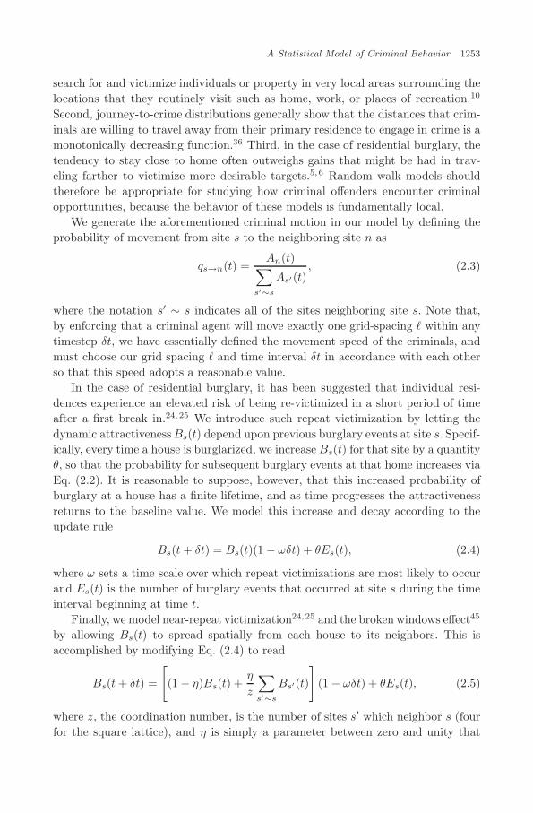
search for and victimize individuals or property in very local areas surrounding thelocations that they routinely visit such as home, work, or places of recreation.10

Second, journey-to-crime distributions generally show that the distances that crim-inals are willing to travel away from their primary residence to engage in crime is amonotonically decreasing function.36 Third, in the case of residential burglary, thetendency to stay close to home often outweighs gains that might be had in trav-eling farther to victimize more desirable targets.5, 6 Random walk models shouldtherefore be appropriate for studying how criminal offenders encounter criminalopportunities, because the behavior of these models is fundamentally local.

We generate the aforementioned criminal motion in our model by defining theprobability of movement from site s to the neighboring site n as

qs→n(t) =An(t)∑

s′∼s

As′(t), (2.3)

where the notation s′ ∼ s indicates all of the sites neighboring site s. Note that,by enforcing that a criminal agent will move exactly one grid-spacing � within anytimestep δt, we have essentially defined the movement speed of the criminals, andmust choose our grid spacing � and time interval δt in accordance with each otherso that this speed adopts a reasonable value.

In the case of residential burglary, it has been suggested that individual resi-dences experience an elevated risk of being re-victimized in a short period of timeafter a first break in.24, 25 We introduce such repeat victimization by letting thedynamic attractiveness Bs(t) depend upon previous burglary events at site s. Specif-ically, every time a house is burglarized, we increase Bs(t) for that site by a quantityθ, so that the probability for subsequent burglary events at that home increases viaEq. (2.2). It is reasonable to suppose, however, that this increased probability ofburglary at a house has a finite lifetime, and as time progresses the attractivenessreturns to the baseline value. We model this increase and decay according to theupdate rule

Bs(t + δt) = Bs(t)(1 − ωδt) + θEs(t), (2.4)

where ω sets a time scale over which repeat victimizations are most likely to occurand Es(t) is the number of burglary events that occurred at site s during the timeinterval beginning at time t.

Finally, we model near-repeat victimization24, 25 and the broken windows effect45

by allowing Bs(t) to spread spatially from each house to its neighbors. This isaccomplished by modifying Eq. (2.4) to read

Bs(t + δt) =

[(1 − η)Bs(t) +

η

z

∑s′∼s

Bs′(t)

](1 − ωδt) + θEs(t), (2.5)

where z, the coordination number, is the number of sites s′ which neighbor s (fourfor the square lattice), and η is simply a parameter between zero and unity that

July 25, 2008 11:25 WSPC/103-M3AS 00302


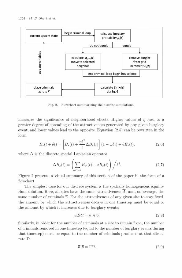
Fig. 2. Flowchart summarizing the discrete simulations.

measures the significance of neighborhood effects. Higher values of η lead to agreater degree of spreading of the attractiveness generated by any given burglaryevent, and lower values lead to the opposite. Equation (2.5) can be rewritten in theform

Bs(t + δt) =[Bs(t) +

η�2

z∆Bs(t)

](1 − ωδt) + θEs(t), (2.6)

where ∆ is the discrete spatial Laplacian operator

∆Bs(t) =

(∑s′∼s

Bs′(t) − zBs(t)

)/�2. (2.7)

Figure 2 presents a visual summary of this section of the paper in the form of aflowchart.

The simplest case for our discrete system is the spatially homogeneous equilib-rium solution. Here, all sites have the same attractiveness A, and, on average, thesame number of criminals n. For the attractiveness of any given site to stay fixed,the amount by which the attractiveness decays in one timestep must be equal tothe amount by which it increases due to burglary events:

ωBδt = θ n p. (2.8)

Similarly, in order for the number of criminals at a site to remain fixed, the numberof criminals removed in one timestep (equal to the number of burglary events duringthat timestep) must be equal to the number of criminals produced at that site atrate Γ:

n p = Γδt. (2.9)

July 25, 2008 11:25 WSPC/103-M3AS 00302


Table 1. Summary of parameters present in the discrete model.

Parameter name Meaning

� Grid spacingδt Time stepω Dynamic attractiveness decay rateη Measures neighborhood effects (ranging from

0 to 1)θ Increase in attractiveness due to one

burglary eventA0

s Intrinsic attractiveness of site sΓ Rate of burglar generation at each site

Putting these two equations together allows us to solve for the homogeneous equi-librium values

B =θΓω

, n =Γδt

1 − e−Aδt. (2.10)

The question of whether or not a system placed in this homogeneous equilibriumstate will remain in it will be answered in our next section.

2.2. Computer simulations

Computer simulations of the model described above follow the general outline asshown in Fig. 2. The main purpose of the simulations is to give insight into thebehavior of the model under various combinations of the many parameters present(see Table 1).

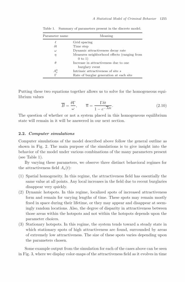
By varying these parameters, we observe three distinct behavioral regimes forthe attractiveness field As(t):

(1) Spatial homogeneity. In this regime, the attractiveness field has essentially thesame value at all points. Any local increases in the field due to recent burglariesdisappear very quickly.

(2) Dynamic hotspots. In this regime, localized spots of increased attractivenessform and remain for varying lengths of time. These spots may remain mostlyfixed in space during their lifetime, or they may appear and disappear at seem-ingly random locations. Also, the degree of disparity in attractiveness betweenthose areas within the hotspots and not within the hotspots depends upon theparameter choices.

(3) Stationary hotspots. In this regime, the system tends toward a steady state inwhich stationary spots of high attractiveness are found, surrounded by areasof extremely low attractiveness. The size of these spots varies depending uponthe parameters chosen.

Some example output from the simulation for each of the cases above can be seenin Fig. 3, where we display color-maps of the attractiveness field as it evolves in time

July 25, 2008 11:25 WSPC/103-M3AS 00302


t = 10 days, 1619 criminals

0

5

0

100


0 50 100


0 50 100 0 50 100

(a)


0

5

0

100


0 50 100


0 50 100 0 50 100

(b)


0

5

0

100


0 50 100


0 50 100 0 50 100

(c)


0

5

0

100


0 50 100


0 50 100 0 50 100

(d)

Fig. 3. Output from the discrete simulation, using parameters described in the text. For the lowcriminal numbers in (b) and (d), we observe dynamic hotspots. Those in (b) are more transientin nature, while those in (d) linger but display large deformations over time. For higher criminalnumbers, we observe either (a) no significant hotspots, or (c) stationary hotspots.

July 25, 2008 11:25 WSPC/103-M3AS 00302


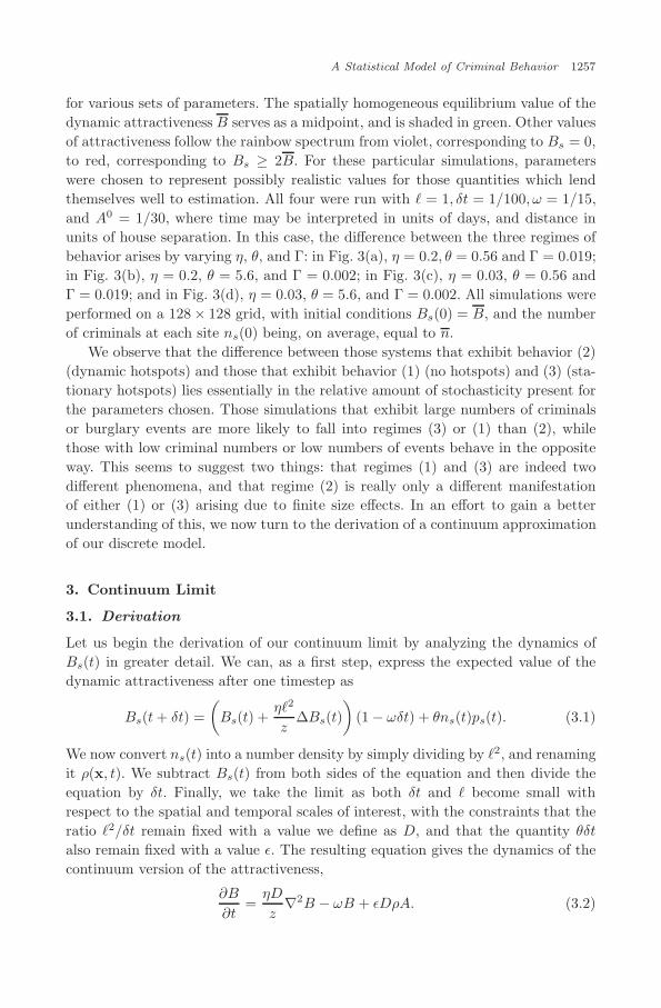
for various sets of parameters. The spatially homogeneous equilibrium value of thedynamic attractiveness B serves as a midpoint, and is shaded in green. Other valuesof attractiveness follow the rainbow spectrum from violet, corresponding to Bs = 0,to red, corresponding to Bs ≥ 2B. For these particular simulations, parameterswere chosen to represent possibly realistic values for those quantities which lendthemselves well to estimation. All four were run with � = 1, δt = 1/100, ω = 1/15,and A0 = 1/30, where time may be interpreted in units of days, and distance inunits of house separation. In this case, the difference between the three regimes ofbehavior arises by varying η, θ, and Γ: in Fig. 3(a), η = 0.2, θ = 0.56 and Γ = 0.019;in Fig. 3(b), η = 0.2, θ = 5.6, and Γ = 0.002; in Fig. 3(c), η = 0.03, θ = 0.56 andΓ = 0.019; and in Fig. 3(d), η = 0.03, θ = 5.6, and Γ = 0.002. All simulations wereperformed on a 128 × 128 grid, with initial conditions Bs(0) = B, and the numberof criminals at each site ns(0) being, on average, equal to n.

We observe that the difference between those systems that exhibit behavior (2)(dynamic hotspots) and those that exhibit behavior (1) (no hotspots) and (3) (sta-tionary hotspots) lies essentially in the relative amount of stochasticity present forthe parameters chosen. Those simulations that exhibit large numbers of criminalsor burglary events are more likely to fall into regimes (3) or (1) than (2), whilethose with low criminal numbers or low numbers of events behave in the oppositeway. This seems to suggest two things: that regimes (1) and (3) are indeed twodifferent phenomena, and that regime (2) is really only a different manifestationof either (1) or (3) arising due to finite size effects. In an effort to gain a betterunderstanding of this, we now turn to the derivation of a continuum approximationof our discrete model.

3. Continuum Limit

3.1. Derivation

Let us begin the derivation of our continuum limit by analyzing the dynamics ofBs(t) in greater detail. We can, as a first step, express the expected value of thedynamic attractiveness after one timestep as

Bs(t + δt) =(

Bs(t) +η�2

z∆Bs(t)

)(1 − ωδt) + θns(t)ps(t). (3.1)

We now convert ns(t) into a number density by simply dividing by �2, and renamingit ρ(x, t). We subtract Bs(t) from both sides of the equation and then divide theequation by δt. Finally, we take the limit as both δt and � become small withrespect to the spatial and temporal scales of interest, with the constraints that theratio �2/δt remain fixed with a value we define as D, and that the quantity θδt

also remain fixed with a value ε. The resulting equation gives the dynamics of thecontinuum version of the attractiveness,

∂B

∂t=

ηD

z∇2B − ωB + εDρA. (3.2)

July 25, 2008 11:25 WSPC/103-M3AS 00302


The derivation of the continuum limit for ns(t) is slightly more involved. Webegin with an equation expressing the expected number of agents at a site after onetimestep, noting that our model demands that all of the agents that were at thesite s at time t must have left the site either by moving to a neighboring site or byburglarizing the site and thereby being removed. Because of this, any agents thatare present after one timestep must have either arrived there from a neighboringsite after failing to burgle the neighbor, or have been generated there at rate Γ.Therefore, we conclude that

ns(t + δt) = As

∑s′∼s

ns′(t) [1 − ps′(t)]Ts′(t)

+ Γδt, (3.3)

where, for sake of notational simplicity, we have defined

Ts′(t) ≡∑

s′′∼s′As′′(t). (3.4)

Now, we perform an operation like that done previously when converting fromEq. (2.5) to (2.6) to write the sum in Eq. (3.3) and Ts′(t) in terms of the discretespatial Laplacian. We then subtract ns(t) from both sides of the equation, re-expressns(t) in terms of ρ(x, t), and divide by δt. Upon taking the limits of � and δt asdescribed previously, with the further constraint that Γ/�2 = γ, we arrive at ourcontinuum equation for criminal number density

∂ρ

∂t=

D

z∇ ·[∇ρ − 2ρ

A∇A

]− ρA + γ. (3.5)

Equations (3.2) and (3.5) are the main results of our continuum derivation, andare of the general form of a reaction-diffusion system; such systems often lead topattern formation.16 The attractiveness diffuses throughout the environment whilesimultaneously decaying in time and reacting with the criminals to create evenmore attractiveness. Criminals are depleted through reactions with the attractive-ness and are created at a constant rate. In addition, the criminals exhibit bothdiffusive motion and advective motion up gradients of attractiveness, with a speedthat is inversely proportional to the local attractiveness field. This can be inter-preted in a sociological sense as an example of diminishing returns; if an offenderis already located at a highly attractive home, it may feel less motivation to moveto neighboring houses that are, relatively speaking, not that much more attractive.

We will now point out two interesting characteristics of our continuum equations(3.2) and (3.5). First, if we integrate the steady-state version of Eq. (3.5) over ourentire spatial domain, we find that the spatially averaged crime rate density is equalto γ, assuming that the criminal flux is either zero at the boundaries or is periodic.Interestingly, this means that all systems with a given γ will exhibit the sameoverall rate of crime at steady state, regardless of whether that crime is or is notconcentrated in hotspots. Secondly, we see by integrating the steady-state versionof Eq. (3.9) over our domain that our homogeneous equilibrium attractiveness value

July 25, 2008 11:25 WSPC/103-M3AS 00302


B is in fact the spatially averaged attractiveness value for any steady-state system.In terms of our continuum parameters, this value is

B =εDγ

ω. (3.6)

So, we can now understand in some sense why the stationary hotspots observedin our discrete simulations appear as they do, surrounded by areas of very lowattractiveness: since the average attractiveness is fixed, areas of high B must bebalanced by areas of low B.

As a final step, let us rewrite Eqs. (3.2) and (3.5) in a dimensionless form. Wefirst note that a natural time scale for our model is given by τ ≡ 1/ω, as discussedpreviously. A characteristic length scale �c can be defined as

�c ≡√

D

ω, (3.7)

which is roughly the distance over which criminal agents diffuse in the time τ ittakes for the attractiveness of a newly burgled house to return to the baseline value.We therefore scale variables in the following way, denoting dimensionless versionswith a tilde:

A = A/ω, ρ = ε�2cρ, x =

√zx/�c, t = ωt. (3.8)

Using these new variables, our continuum equations can be re-expressed, now drop-ping the tilde notation, as

∂B

∂t= η∇2B − B + ρA, and (3.9)

∂ρ

∂t= ∇ ·

[∇ρ − 2ρ

A∇A

]− ρA + B, (3.10)

where B should be understood as the dimensionless version of Eq. (3.6). Note at thispoint that we have now transformed our original discrete system with seven param-eters into a dimensionless continuum version that has only three free parameters:η, A0, and B.

Deriving continuum equations from the underlying microscale behavior of asystem is a common procedure in mathematical biology.3, 4, 14, 15, 18, 19, 22, 33, 39 Itis no surprise, then, that Eqs. (3.9) and (3.10) are related to several otherwell-studied models. One particular model, which has a large literature inapplied mathematics, is the Keller–Segel model for aggregation based on chemo-taxis.12, 13, 17, 20, 23, 28, 30, 38, 40, 43 In our model, the decay of attractiveness in Eq. (3.9)includes the time derivative, which is typically suppressed in the chemotaxis mod-els. This is because the timescale of change of attractiveness can be comparable tothat of the motion of criminals, unlike in the chemotaxis problem. Moreover, in ourproblem we consider a decay of criminal density once crimes have occured, which isalso not present in typical chemotaxis models. It would be interesting to considersome basic questions such as global existence of solutions and long-time behavior

July 25, 2008 11:25 WSPC/103-M3AS 00302



0 50 100

0

5

0

100


0 50 100 0

50

1

00


0 50 100

0

5

0

100

(a) (b) (c)

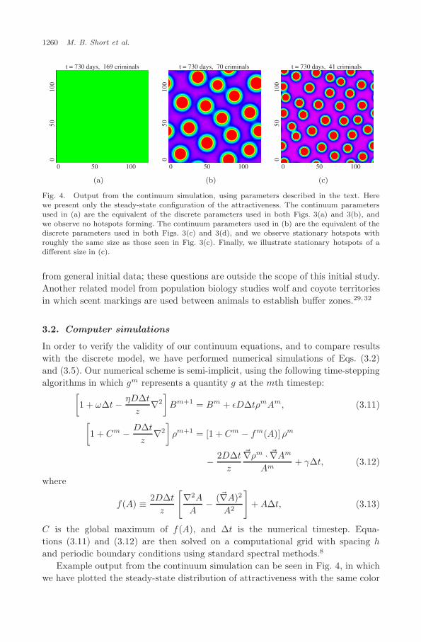
Fig. 4. Output from the continuum simulation, using parameters described in the text. Herewe present only the steady-state configuration of the attractiveness. The continuum parametersused in (a) are the equivalent of the discrete parameters used in both Figs. 3(a) and 3(b), andwe observe no hotspots forming. The continuum parameters used in (b) are the equivalent of thediscrete parameters used in both Figs. 3(c) and 3(d), and we observe stationary hotspots withroughly the same size as those seen in Fig. 3(c). Finally, we illustrate stationary hotspots of adifferent size in (c).

from general initial data; these questions are outside the scope of this initial study.Another related model from population biology studies wolf and coyote territoriesin which scent markings are used between animals to establish buffer zones.29, 32

3.2. Computer simulations

In order to verify the validity of our continuum equations, and to compare resultswith the discrete model, we have performed numerical simulations of Eqs. (3.2)and (3.5). Our numerical scheme is semi-implicit, using the following time-steppingalgorithms in which gm represents a quantity g at the mth timestep:[

1 + ω∆t − ηD∆t

z∇2

]Bm+1 = Bm + εD∆tρmAm, (3.11)

[1 + Cm − D∆t

z∇2

]ρm+1 = [1 + Cm − fm(A)] ρm

− 2D∆t

z

∇ρm · ∇Am

Am+ γ∆t, (3.12)

where

f(A) ≡ 2D∆t

z

[∇2A

A− (∇A)2

A2

]+ A∆t, (3.13)

C is the global maximum of f(A), and ∆t is the numerical timestep. Equa-tions (3.11) and (3.12) are then solved on a computational grid with spacing h

and periodic boundary conditions using standard spectral methods.8

Example output from the continuum simulation can be seen in Fig. 4, in whichwe have plotted the steady-state distribution of attractiveness with the same color

July 25, 2008 11:25 WSPC/103-M3AS 00302


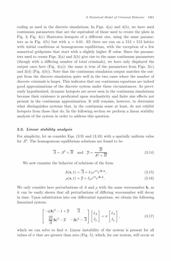
coding as used in the discrete simulations. In Figs. 4(a) and 4(b), we have usedcontinuum parameters that are the equivalent of those used to create the plots inFig. 3; Fig. 4(c) illustrates hotspots of a different size, using the same parame-ters as in Fig. 4(b) but with η = 0.01. All three are run on a 512 × 512 latticewith initial conditions at homogeneous equilibrium, with the exception of a fewnumerical gridpoints that start with a slightly higher B value. Since the parame-ters used to create Figs. 3(a) and 3(b) give rise to the same continuum parameters(though with a differing number of total criminals), we have only displayed theoutput once here (Fig. 4(a)); the same is true of the parameters from Figs. 3(c)and 3(d) (Fig. 4(b)). Note that the continuum simulation output matches the out-put from the discrete simulation quite well in the two cases where the number ofdiscrete criminals is larger. This indicates that our continuum equations are indeedgood approximations of the discrete system under these circumstances. As previ-ously hypothesized, dynamic hotspots are never seen in the continuum simulationsbecause their existence is predicated upon stochasticity and finite size effects notpresent in the continuum approximation. It still remains, however, to determinewhat distinguishes systems that, in the continuum sense at least, do not exhibithotspots from those that do. In the following section we perform a linear stabilityanalysis of the system in order to address this question.

3.3. Linear stability analysis

For simplicity, let us consider Eqs. (3.9) and (3.10) with a spatially uniform valuefor A0. The homogeneous equilibrium solutions are found to be

A = A0 + B and ρ =B

A0 + B. (3.14)

We now examine the behavior of solutions of the form

A(x, t) = A + δAeσteik·x, (3.15)

ρ(x, t) = ρ + δρeσteik·x. (3.16)

We only consider here perturbations of A and ρ with the same wavenumber k, asit can be easily shown that all perturbations of differing wavenumber will decayin time. Upon substitution into our differential equations, we obtain the followinglinearized system:

−η|k|2 − 1 + ρ A

2ρ

A|k|2 − ρ −|k|2 − A

[

δA

δρ

]= σ

[δA

δρ

], (3.17)

which we can solve to find σ. Linear instability of the system is present for allvalues of σ that are greater than zero (Fig. 5), which, for our system, will occur at

July 25, 2008 11:25 WSPC/103-M3AS 00302


1 2 3|k*|2 4

Wavenumber Squared, |k|2-1

-0.5

0

0.5

1

Gro

wth

Rat

e, σ

Real ComponentImaginary Component

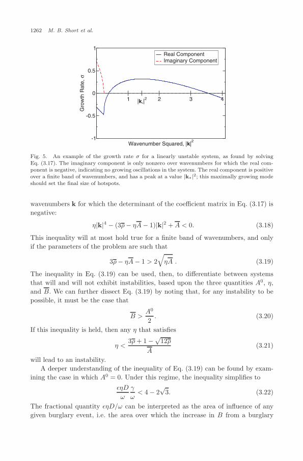
Fig. 5. An example of the growth rate σ for a linearly unstable system, as found by solvingEq. (3.17). The imaginary component is only nonzero over wavenumbers for which the real com-ponent is negative, indicating no growing oscillations in the system. The real component is positiveover a finite band of wavenumbers, and has a peak at a value |k∗|2; this maximally growing modeshould set the final size of hotspots.

wavenumbers k for which the determinant of the coefficient matrix in Eq. (3.17) isnegative:

η|k|4 − (3ρ − ηA − 1)|k|2 + A < 0. (3.18)

This inequality will at most hold true for a finite band of wavenumbers, and onlyif the parameters of the problem are such that

3ρ− ηA − 1 > 2√

ηA . (3.19)

The inequality in Eq. (3.19) can be used, then, to differentiate between systemsthat will and will not exhibit instabilities, based upon the three quantities A0, η,and B. We can further dissect Eq. (3.19) by noting that, for any instability to bepossible, it must be the case that

B >A0

2. (3.20)

If this inequality is held, then any η that satisfies

η <3ρ + 1 −√

12ρ

A(3.21)

will lead to an instability.A deeper understanding of the inequality of Eq. (3.19) can be found by exam-

ining the case in which A0 = 0. Under this regime, the inequality simplifies to

εηD

ω

γ

ω< 4 − 2

√3. (3.22)

The fractional quantity εηD/ω can be interpreted as the area of influence of anygiven burglary event, i.e. the area over which the increase in B from a burglary

July 25, 2008 11:25 WSPC/103-M3AS 00302


0.02 0.04 0.06 0.08η

20

30

40

50

Dis

tanc

e B

etw

een

Spo

ts, λ

*

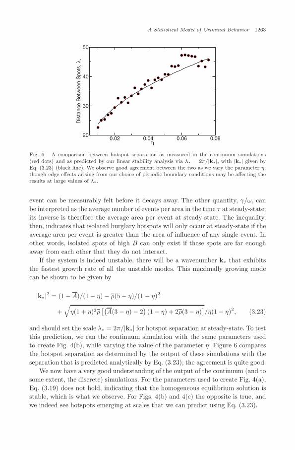
Fig. 6. A comparison between hotspot separation as measured in the continuum simulations(red dots) and as predicted by our linear stability analysis via λ∗ = 2π/|k∗|, with |k∗| given byEq. (3.23) (black line). We observe good agreement between the two as we vary the parameter η,though edge effects arising from our choice of periodic boundary conditions may be affecting theresults at large values of λ∗.

event can be measurably felt before it decays away. The other quantity, γ/ω, canbe interpreted as the average number of events per area in the time τ at steady-state;its inverse is therefore the average area per event at steady-state. The inequality,then, indicates that isolated burglary hotspots will only occur at steady-state if theaverage area per event is greater than the area of influence of any single event. Inother words, isolated spots of high B can only exist if these spots are far enoughaway from each other that they do not interact.

If the system is indeed unstable, there will be a wavenumber k∗ that exhibitsthe fastest growth rate of all the unstable modes. This maximally growing modecan be shown to be given by

|k∗|2 = (1 − A)/(1 − η) − ρ(5 − η)/(1 − η)2

+√

η(1 + η)2ρ[(

A(3 − η) − 2)(1 − η) + 2ρ(3 − η)

]/η(1 − η)2, (3.23)

and should set the scale λ∗ = 2π/|k∗| for hotspot separation at steady-state. To testthis prediction, we ran the continuum simulation with the same parameters usedto create Fig. 4(b), while varying the value of the parameter η. Figure 6 comparesthe hotspot separation as determined by the output of these simulations with theseparation that is predicted analytically by Eq. (3.23); the agreement is quite good.

We now have a very good understanding of the output of the continuum (and tosome extent, the discrete) simulations. For the parameters used to create Fig. 4(a),Eq. (3.19) does not hold, indicating that the homogeneous equilibrium solution isstable, which is what we observe. For Figs. 4(b) and 4(c) the opposite is true, andwe indeed see hotspots emerging at scales that we can predict using Eq. (3.23).

July 25, 2008 11:25 WSPC/103-M3AS 00302


4. Conclusions

We re-emphasize at this point that the model described herein has been constructedbased upon the empirically known behavior of criminal offenders. First, based onthe fact that burglars most often victimize areas near where they live, work, orspend free time, we have chosen to model their movement as a biased random walk,as the behavior of such a model is fundamentally local in space. Second, as it isclear that repeat victimization plays an important role in crime pattern generation,we have developed the idea of an attractiveness field that not only determines therate of burglary at a given site, but is also influenced by past burglary events andserves as the source of bias in the criminals’ movement. Finally, we have introducedspatio-temporal scales for hotspots by allowing our attractiveness field to diffusewithin a neighborhood while simultaneously decaying in time. We thus are ableto construct a model where the two main variables at play, offender position (ordensity in the continuum model), and biasing attractiveness field, create nonlinearfeedback loops which originate patterns of aggregation, reminiscent of actual crimehotspots.

This sociologically based model accomplishes our chief goal of exhibiting qual-itative similarity with the hotspots observed in actual cities. However, there hasbeen no comparison as of yet between the quantitative aspects of the hotspots gen-erated thereby and empirical crime data. This is partly because of the difficulty indeveloping a rigorous metric by which such a comparison could be made. To wit,there are numerous quantities that can be measured in both our simulation outputand empirical burglary data that could serve as such a rubric: the probability dis-tribution for number of burglaries per house over a prescribed period of time, thedistribution of time to next event for houses within a fixed distance of a burglaryevent, any number of tests for spatiotemporal clustering of burglary events, etc.Choosing which one of these measures to focus our attention toward is a work inprogress.

In addition to this difficulty in determining the appropriate metric for compar-ison is the fact that there are other variables acting within the empirical data thatare not accounted for in the model, e.g. police presence and other security mea-sures. It is a fact that police departments often distribute crime control resourcesbased upon recent criminal activity, which may shorten the lifetime of hotspots,cause them to relocate, or destroy them altogether. Despite these many difficulties,however, we feel confident that the parameters of our model could be chosen to givegood agreement between simulation and real data.

Another area of further inquiry involves incorporating inhomogeneities into thecomputer simulations. For example, it would be very interesting to construct thebackground attractiveness field A0 or the burglar generation rate Γ by taking intoaccount the characteristics of a specific city location (neighborhood income lev-els, security measures installed, proximity to crime generating or deterring centers,physical hindrances to the spread of A, police response times and methods). In a

July 25, 2008 11:25 WSPC/103-M3AS 00302


similar vein, constructing realistic urban lattices upon which to run our simula-tions will be very important in the future, and allow for much better comparisonsbetween the simulation and data, as well as possibly providing enhanced predictivecapability.

In the end, we feel that the ideas presented here will form the basis for a betterunderstanding of why and how crime hotspots form and of their underlying dynam-ics. This knowledge may eventually prove useful for developing better methods ofcrime prediction and prevention and allow the police and other security agencies tomore effectively control resource allocation from day to day.

Acknowledgments

The authors wish to thank the Los Angeles and Long Beach police departments,Joe Kuhns of the LAPD, Roy Stone of the LBPD, and Tom Chou of UCLA forhelpful discussions, NSF grants BCS-0527388 and DMS-0719462, and ARO grantMURI-50363-MA-MUR.

References

1. L. Anselin, J. Cohen, D. Cook, W. Gorr and G. Tita, Criminal Justice 2000, Vol. 4(National Institute of Justice, 2000), pp. 213–262.

2. D. Beavon, P. L. Brantingham and P. J. Brantingham, Crime Prevention Studies,Vol. 2 (Willow Tree Press, 1994), pp. 115–148.

3. N. Bellomo, A. Bellouquid, J. Nieto and J. J. Soler, Multicellular growing systems:Hyperbolic limits towards macroscopic description, Math. Mod. Meth. Appl. Sci. 17(2007) 1675–1693.

4. M. Bendahmame, K. H. Karlsen and J. M. Urbano, On a two-sidely degenerate chemo-taxis model with volume-filling effects, Math. Mod. Meth. Appl. Sci. 17 (2007) 783–804.

5. W. Bernasco and F. Luykx, Effects of attractiveness, opportunity and accessibility toburglars on residential burglary rates of urban neighborhoods, Criminology 41 (2003)981–1001.

6. W. Bernasco and P. Nieuwbeerta, How do residential burglars select target areas?A new approach to the analysis of criminal location choice, Brit. J. Criminology 45(2005) 296–315.

7. A. E. Bottoms and P. Wiles, Crime, Policing and Place: Essays in EnvironmentalCriminology (Routledge, 1992), pp. 11–35.

8. J. P. Boyd, Chebyshev and Fourier Spectral Methods, 2nd edn. (Dover, 2001).9. P. J. Brantingham and P. L. Brantingham, Patterns in Crime (Macmillan, 1984).

10. P. J. Brantingham and P. L. Brantingham, Environmental Criminology, 2nd edn.(Waveland Press, 1991), pp. 27–54.

11. P. J. Brantingham and P. L. Brantingham, Criminality of place: Crime generatorsand crime attractors, Euro. J. Criminal Policy Res. 3 (1995) 5–26.

12. M. Burger, M. Di Francesco and Y. Dolak-Struss, The Keller–Segel model for chemo-taxis with prevention of overcrowding: Linear vs. nonlinear diffusion, SIAM J. Math.Anal. 38 (2006) 1288–1315.

13. H. M. Byrne and M. R. Owen, A new interpretation of the Keller–Segel model basedon multiphase modelling, J. Math. Biol. 49 (2004) 604–626.

July 25, 2008 11:25 WSPC/103-M3AS 00302


14. F. A. Chalub, Y. Dolak-Struss, P. Markowich, D. Oeltz, C. Schmeiser and A. Soref,Model hierarchies for cell aggregation by chemotaxis, Math. Mod. Meth. Appl. Sci.16 (2006) 1173.

15. F. A. Chalub, P. A. Markovich, B. Perthame and C. Schmeiser, Kinetic models forchemotaxis and their drift-diffusion limits, Mon. Math. 142 (2004) 123.

16. M. C. Cross and P. C. Hohenberg, Pattern formation outside of equilibrium, Rev.Mod. Phys. 65 (1993) 851–1112.

17. M. del Pino and J. Wei, Collapsing steady states of the Keller–Segel system, Nonlin-earity 19 (2006) 661–684.

18. Y. Dolak and C. Schmeiser, Kinetic models for chemotaxis: Hydrodynamic limits andspatio temporal mechanisms, J. Math. Biol. 51 (2005) 595–615.

19. R. Erban and H. G. Othmer, From individual to collective behaviour in chemotaxis,SIAM J. Appl. Math. 65 (2004) 361–391.

20. C. Escudero, The fractional Keller–Segel model, Nonlinearity 19 (2006) 2909–2918.21. M. K. Felson, Crime and Nature (Sage Publications, 2006).22. F. Filbet, P. Laurencot and B. Perthame, Derivation of hyperbolic models for

chemosensitive movement, J. Math. Biol. 50 (2005) 189–207.23. M. A. Herrero and J. J. L. Velazquez, Chemotactic collapse for the Keller–Segel model,

J. Math. Biol. 35 (1996) 177–194.24. S. D. Johnson, W. Bernasco, K. J. Bowers, H. Elffers, J. Ratcliffe, G. Rengert and

M. Townsley, Space-time patterns of risk: A cross national assessment of residentialburglary victimization, J. Quantitative Criminology 23 (2007) 201–219.

25. S. D. Johnson, K. Bowers and A. Hirschfield, New insights into the spatial and tem-poral distribution of repeat victimisation, Br. J. Criminology 37 (1997) 224–244.

26. S. D. Johnson and K. J. Bowers, The burglary as clue to the future: The beginningsof prospective hot-spotting, Eur. J. Criminology 1 (2004) 237–255.

27. S. D. Johnson and K. J. Bowers, Domestic burglary repeats and space-time clusters:The dimensions of risk, Eur. J. Criminology 2 (2005) 67–92.

28. E. F. Keller and L. A. Segel, Initiation of slime mold aggregation viewed as an insta-bility, J. Theor. Biol. 26 (1970) 399–415.

29. M. A. Lewis, K. A. J. White and J. D. Murray, Analysis of a model for wolf territories,J. Math. Biol. 35 (1997) 749–774.

30. S. Luckhaus and Y. Sugiyama, Large time behavior of solutions in super-critical casesto degenerate Keller–Segel systems, Math. Model. Numer. Anal. 40 (2006) 597–621.

31. L. McLaughlin, S. D. Johnson, D. Birks, K. J. Bowers and K. Pease, Police perceptionsof the long and short term spatial distribution of residential burglary, Int. J. PoliceSci. Management 9 (2007) 99–111.

32. P. R. Moorcroft, M. A. Lewis and R. Crabtree, Mechanistic home range models predictpatterns of coyote territories in yellowstone, Proc. Roy. Soc. London B 273 (2006)1651–1659.

33. H. G. Othmer and T. Hillen, The diffusion limit of transport equations II: Chemotaxisequations, SIAM J. Appl. Math. 62 (2002) 1222–1250.

34. J. H. Ratcliffe, Crime mapping and the training needs of law enforcement, Eur. J.Criminal Policy Res. 10 (2004) 65–83.

35. G. F. Rengert, Crime, Policing and Place: Essays in Environmental Criminology(Routledge, 1992), pp. 109–117.

36. G. F. Rengert, A. R. Piquero and P. R. Jones, Distance decay reexamined, Criminology37 (1999) 427–445.

37. D. Roncek and R. Bell, Bars, blocks and crime, J. Environ. Sys. 11 (1981) 35–47.

July 25, 2008 11:25 WSPC/103-M3AS 00302


38. T. Senba, Type II blowup of solutions to a simplified Keller–Segel system in two-dimensional domains, Nonlinear Anal. Th. Meth. Appl. Int. Multidisciplinary J. Ser.A: Th. Meth. 66 (2007) 1817–1839.

39. A. Stevens, The derivation of chemotaxis equations as limit dynamics of moder-ately interacting stochastic many-particles systems, SIAM J. Appl. Math. 61 (2002)183–212.

40. Y. Sugiyama, Global existence in sub-critical cases and finite time blow-up in super-critical cases to degenerate Keller–Segel systems, Differential and Integral Equations.Int. J. Th. Appl. 19 (2006) 841–876.

41. G. Tita, J. Cohen and J. Engberg, An ecological study of the location of gang “setspace,” Social Problems 52 (2005) 272–299.

42. G. Tita and G. Ridgeway, The impact of gang formation on local patterns of crime,J. Res. Crime Delinquency 44 (2007) 208–237.

43. J. J. L. Velazquez, Well-posedness of a model of point dynamics for a limit of theKeller–Segel system, J. Diff. Eqs. 206 (2004) 315–352.

44. W. F. Walsh, Compstat: An analysis of an emerging police managerial paradigm,Policing 24 (2001) 347–362.

45. J. Q. Wilson and G. L. Kelling, Broken windows and police and neighborhood safety,Atlantic Mon. 249 (1982) 29–38.

46. R. Wright and S. Decker, Burglars on the Job (Northeastern Univ. Press, 1994).

Documents

July 25, 2008 11:25 WSPC/103-M3AS 00302 …lchayes/lchayes_website_folder/new...July 25, 2008 11:25 WSPC/103-M3AS 00302 Mathematical Models and Methods in Applied Sciences Vol. 18,