Faculty of Natural Sciences and Technology I

Department of Computer Science

Master‘s Thesis

Race time prediction on individual historical training data for hilly and non-hilly courses

Julian MaurerMaster‘s Program of Media Informatics

March 2018

II

Advisors:Dr.-Ing. Florian Daiber,German Research Center for Artificial Intelligence, Saarbrücken, GermanyFrederik Wiehr,German Research Center for Artificial Intelligence, Saarbrücken, Germany

Supervisor:Prof. Dr. Antonio Krüger,German Research Center for Artificial Intelligence, Saarbrücken, Germany

Reviewers:Prof. Dr. Antonio Krüger,German Research Center for Artificial Intelligence, Saarbrücken, GermanyDr.-Ing. Boris Brandherm,German Research Center for Artificial Intelligence, Saarbrücken, Germany

Submitted20. March 2018

Saarland UniversityFaculty of Natural Sciences and Technology IDepartment of Computer ScienceCampus - Building E1.166123 SaarbrückenGermany

III

Statement in Lieu of an Oath:

I hereby confirm that I have written this thesis on my own and that I have not used any other media or materials than the ones referred to in this thesis.

Saarbrücken, 20th of March, 2018

Declaration of Consent:

I agree to make both versions of my thesis (with a passing grade) accessible to the pub-lic by having them added to the library of the Computer Science Department.

Saarbrücken, 20th of March, 2018

IV

Acknowledgments

I sincerely thank Prof. Dr. Antonio Krüger for giving me the opportunity to write this thesis under his supervision. Furthermore, I would like to thank Dr.-Ing. Boris Brand-herm for reviewing my thesis.Special thanks goes to my two advisors Florian Daiber and Frederik Wiehr who helped me to find such an interesting topic, gave valuable advice and spend many hours of discussion with me.In addition, I would like to thank all athletes who participated in my studies and pro-vided their personal training data.Lastly, I want to thank my family who have supported me throughout the entire pro-cess.

V

Abstract

Running is a popular sport pursued by millions of people and not only reserved for the elite or the professionals but for recreational runners and beginners. Tracking workouts to upload them to the internet and share them with others has become a trend. Tracked training sessions reveal lots of information about the fitness of an athlete. Coaches and runners can use this information to make predictions for upcoming races. Most of the available predictions tools use standard formulas obtained by analyzing times of elite runners on flat tracks, but only a few incorporate elevation changes. We examined newer methods in related work to get inspired by excellent results using more athlete specific training data for predictions. There is a tendency to go away from elite based predictions to individualized predictions including multiple training parameters for any kind of races in terms of distance and terrain. Motivated by an online question-naire, we presented two approaches for race time prediction on historical training data of athletes. The first approach looks at the activities as a whole to extract the features for prediction, while the second one breaks down each activity into segments to give a better representation of the underlying elevation profile. The first approach achieved an average accuracy of 91.28 %, while the second model performed slightly worse with an accuracy of 89.82 %. In a user study, the first model achieved even better results with an average accuracy of 95.25 %. Evaluation has shown that both models are able to adapt race time depending on the amount of elevation changes.

VI

Contents

1 Introduction 11.1 Motivation . . . . . . . . . . . . . . . . . . . . . . . . . . . . . . . . . . . . . . . . . . . . . . . . . . . . . . . . . . . 11.2 Research goals and outline . . . . . . . . . . . . . . . . . . . . . . . . . . . . . . . . . . . . . . . . . . . 2

2 Related work 32.1 Power models, scoring tables and other formulas . . . . . . . . . . . . . . . . . . . . . . 32.2 More complex models using individual historical parameters . . . . . . . . . 62.3 Comparison to our approach . . . . . . . . . . . . . . . . . . . . . . . . . . . . . . . . . . . . . . . . . . 8

3 Survey 103.1 Overview of the questionnaire . . . . . . . . . . . . . . . . . . . . . . . . . . . . . . . . . . . . . . . 103.2 Results . . . . . . . . . . . . . . . . . . . . . . . . . . . . . . . . . . . . . . . . . . . . . . . . . . . . . . . . . . . . . . 123.3 Discussion . . . . . . . . . . . . . . . . . . . . . . . . . . . . . . . . . . . . . . . . . . . . . . . . . . . . . . . . . . 18

4 Implementation 194.1 Historical training data . . . . . . . . . . . . . . . . . . . . . . . . . . . . . . . . . . . . . . . . . . . . . . 204.2 Neural network as a regression model . . . . . . . . . . . . . . . . . . . . . . . . . . . . . . . 294.3 Race time prediction with neural network . . . . . . . . . . . . . . . . . . . . . . . . . . . 324.4 Evaluation . . . . . . . . . . . . . . . . . . . . . . . . . . . . . . . . . . . . . . . . . . . . . . . . . . . . . . . . . . 364.5 Comparison of the two approaches . . . . . . . . . . . . . . . . . . . . . . . . . . . . . . . . . . . 40

5 User study 415.1 Setting and participants . . . . . . . . . . . . . . . . . . . . . . . . . . . . . . . . . . . . . . . . . . . . . 415.2 Method and results . . . . . . . . . . . . . . . . . . . . . . . . . . . . . . . . . . . . . . . . . . . . . . . . . . 425.3 Discussion and improvement . . . . . . . . . . . . . . . . . . . . . . . . . . . . . . . . . . . . . . . . 46

6 Conclusion 536.1 Summary . . . . . . . . . . . . . . . . . . . . . . . . . . . . . . . . . . . . . . . . . . . . . . . . . . . . . . . . . . . 486.2 Evaluation of the overall goal . . . . . . . . . . . . . . . . . . . . . . . . . . . . . . . . . . . . . . . . 496.3 Future work . . . . . . . . . . . . . . . . . . . . . . . . . . . . . . . . . . . . . . . . . . . . . . . . . . . . . . . . . 50

Bibliography 53

VII

List of Figures

2.1 Least squares running curve [21] .......................................................................42.2 PB improvements by Smyth et. al [25] ..............................................................83.1 Age groups, survey .......................................................................................... 103.2 Mileage and races, survey ............................................................................... 123.3 Types of races, survey ..................................................................................... 133.4 Running experience level, survey .................................................................... 143.5 Personal records, survey .................................................................................. 143.6 Problems in races, survey ................................................................................ 153.7 Benefit of application, survey .......................................................................... 173.8 Likeliness of usage, survey .............................................................................. 174.1 High-level system architecture ........................................................................ 194.2 Elevation profile from Strava and Google ....................................................... 214.3 Smoothed elevation profile ..............................................................................224.4 Climbs found in elevation profile ....................................................................234.5 Training Stress Balance model ........................................................................254.6 Grade adjusted pace model ..............................................................................284.7 Architecture of neural network ........................................................................294.8 K-means clustering of activities ....................................................................... 324.9 Elevation gain vs. velocity graph ..................................................................... 334.10 VO2max vs. NGP graph ...................................................................................344.11 Mileage and races, evaluation ..........................................................................364.12 Accuracies and RMSEs, evaluation ................................................................. 374.13 Histogram of prediction errors, evaluation ...................................................... 384.14 Accuracies and similarities, evaluation ........................................................... 394.15 Histogram of segment prediction errors, evaluation ........................................395.1 Number of races, user study ............................................................................ 425.2 Prediction errors Riegel‘s formula, user study ................................................ 435.3 Accuracies and errors, user study ....................................................................445.4 Accuracies and similarities, user study ........................................................... 455.5 Elevation profile and prediction errors of single athlete, user study ................465.6 Predicted time vs. actual time, user study ....................................................... 47

1

1 Introduction

This master thesis presents two approaches to predict performance times for races based on the analysis of historical training data of the individual runner and subse-quent prediction. Elevation changes and other meaningful factors are modelled as fea-tures and fed into a neural network. The trained network is able to predict race times for the athlete on any given race that is available as GPS coordinates.

1.1 MotivationRunning is a popular sport pursued by millions of people around the world. It is not only reserved for the elite or the professionals but for recreational runners and begin-ners who just want to start exercising. In 2016 almost 17 million athletes finished a race in the United States1. With increasing numbers, running had made its way into the tech industry and the internet. People use running watches to track their workouts, upload them to the internet and share them with other athletes. Strava is a website that gained enormous popularity in the last years not only in the running community but for all kinds of athletes. Strava provides a platform for athletes to upload tracking data for various activities. In 2015 people uploaded more than 50 million runs to Strava including more than 275,000 finished marathons2. In 2017 Strava could increase that number to 136 million running related uploads with more than 627,000 finished marathons3. Strava adds a social aspect with giving the opportunity to share all of the uploaded activities with other athletes and compete against them. Motivation enhancement, improved performances evoked by gamification, social net-working and classical training logging gets unified in one platform. Running is no longer a thing that you do on your own but you share it on the internet to receive kudos and motivation. A big advantage of Strava is the opportunity to upload tracking data from all kind of different device brands and to synchronize other services with a Strava account. That is a reason why it serves in this thesis as a source for the training data. Pacing strategies have been a topic in research for a long time and various people in-vestigated how different strategies influenced the overall race performance [11,12,17] or even how wrong distance feedback changed the individual performance [9]. Espe-cially, when running over undulating or mountainous terrain a pacing plan gets more important. The Boston Marathon is just one example, where elevation changes make a strict pacing strategy necessary to achieve similar results like elite runners do4. An still open research question is how the huge amount of tracking data can be used to understand the training process better and help to design assistive technologies. One part is the representation of the state of an athlete in terms of fitness, endurance vs. speed, capability to climb hills, and fatigue. Using this parameters, a coach could suggest a racing plan to an athlete that probably would lead to a good performance.

1 http://www.runningusa.org/2017-us-road-race-trends2 https://www.active.com/triathlon/articles/2015-strava-year-in-review?page=13 https://blog.strava.com/de/2017-in-stats/4 https://medium.com/running-with-data/how-to-pace-like-an-elite-in-boston-4abf26e64bf8

2

But could a computer learn how an athlete races and in the optimal case how he could achieve a new personal record? Runners tend to start races too fast and get slower at the end due to overpacing and fatigue, especially beginners. An application that out-puts a pacing plan for a race, that guides the runner via his running watch during a race would prevent overpacing and help to achieve better times. Part of a pacing plan is the estimation of a target time for the overall race. Predicting a time that a runner needs to finish a race is already a big contribution. Most available race time predictors openly accessible either do not predict on historical training data nor include elevation changes into the prediction. After reviewing related work in the field of performance prediction in running, we decided to set the focus of the thesis to race time prediction on historical training data. Since elevation changes have been very poorly addressed in research, we saw an advantage in including them into the predictions. In the second approach we even investigated if a splitting of the activities into gradient based segments would lead to better predictions.

1.2 Research goals and outlineThe goal of the thesis is to provide a method to predict race times more accurately than current predictors available. An important aspect in our prediction method is the influence of elevation on the predicted time. Our model, which is a neural network should be able to select the relevant features from the input and give a prediction with high accuracy. The goal is to predict more precise times than a baseline, in this case Riegel’s formula [22]. To reach that goal, we introduce two new approaches. The first approach looks at the activity as a whole and computes activity-based features while the second approach splits the activity in segments based on the elevation profile and predicts times for segments. The segment predictions can be reassembled again to get the activity time. Both approaches incorporate elevation gain. The question is, if just knowing the elevation gain and how it is distributed over the course is enough or if a breakdown to gradient based segments gives a better image of the elevation profile and therefore better predictions. First we examined related work in the area of race time prediction and how state-of-the-art predictors perform in terms of accuracy or error. Then we present the results of a survey to better understand the runner’s needs and to show the demands of more accurate prediction tools. As main contribution we introduce two approaches to predict race time and the methodology how to implement them. We start with the analysis of the data and the extraction of the features. Then we briefly describe the model, an un-derlying neural network, to perform the regression task. At the end of the main part we evaluate both models in terms of accuracy using sample data from athletes. To test the models in a real world scenario, we evaluated the proposed approaches in a user study and present the results in the 5th chapter. An overall evaluation of the achieved goals and some ideas for future work conclude the thesis.

1.1 Motivation

3

2 Related work

In the following chapter related work in the area of race time prediction is investigated and summarized. We show some standard approaches based on times of elite runners and some newer approaches based on more athlete specific factors and training data. After presenting the most interesting works, we discuss the advantages and shortcom-ings and compare them to our approaches.

2.1 Power models, scoring tables and other formulasRiegel [22] showed 1981 how the relationship between time and distance in human locomotion can be expressed in a simple formula. He obtained world record times for various forms of endurance sport and put time vs. distance into relation on a large log-log (logarithm) graph. All included sports showed a strong linear relationship from 3.5 to 230 minutes duration. He argued that activities under 3.5 minutes duration include sprint processes and therefore lose their linearity, and all activities lasting longer than 230 minutes get strongly affected by energy depletion and fatigue – plus world class athletes usually focus on standard olympic distances lasting a shorter period of time. He fitted the log of time vs. distance using least-squares technique and found a simple power function, the well known “endurance equation” of the form t = axb where t = time, x = distance and a and b are constants. The constant a has no significant rel-evance because he used it just as a measurement for the units and relative speed. The exponent b represents the “fatigue factor”, the amount a runner’s velocity decreases with increasing distance. He found b to be 1.08 for men and women, and between 1.05 and 1.06 for men between 40 and 70 years old. The following formula can be used to predict times for a race at a given distance based on a previous personal best. T2 is the time to predict, T1 the old personal best, D1 the distance of that record and D2 the dis-tance you want to predict for.

Riegel explicitly stated in his paper that all running records were set on tracks except for marathon. Since the equation was found by using world class reference data the question arises if this equation is applicable for ordinary runners. However, Riegel found out in a informal survey that people running at 70 % of world-class speed at one distance are able to run at 70 % of world-class speed at every other distance. Since he published the paper his formula is referenced worldwide and very often used in predic-tors on the internet. Runner’s World race time calculator used for a long time Riegel’s formula but 2016 they rebuilt it to a more accurate formula predicting marathon times differently. The rebuilt was derived from a research paper published by Vickers et al. [28] showing the failure of the Riegel formula in predicting marathon times for recreational runners. They conducted a study for recreational runners instead of elite runners and collected

4

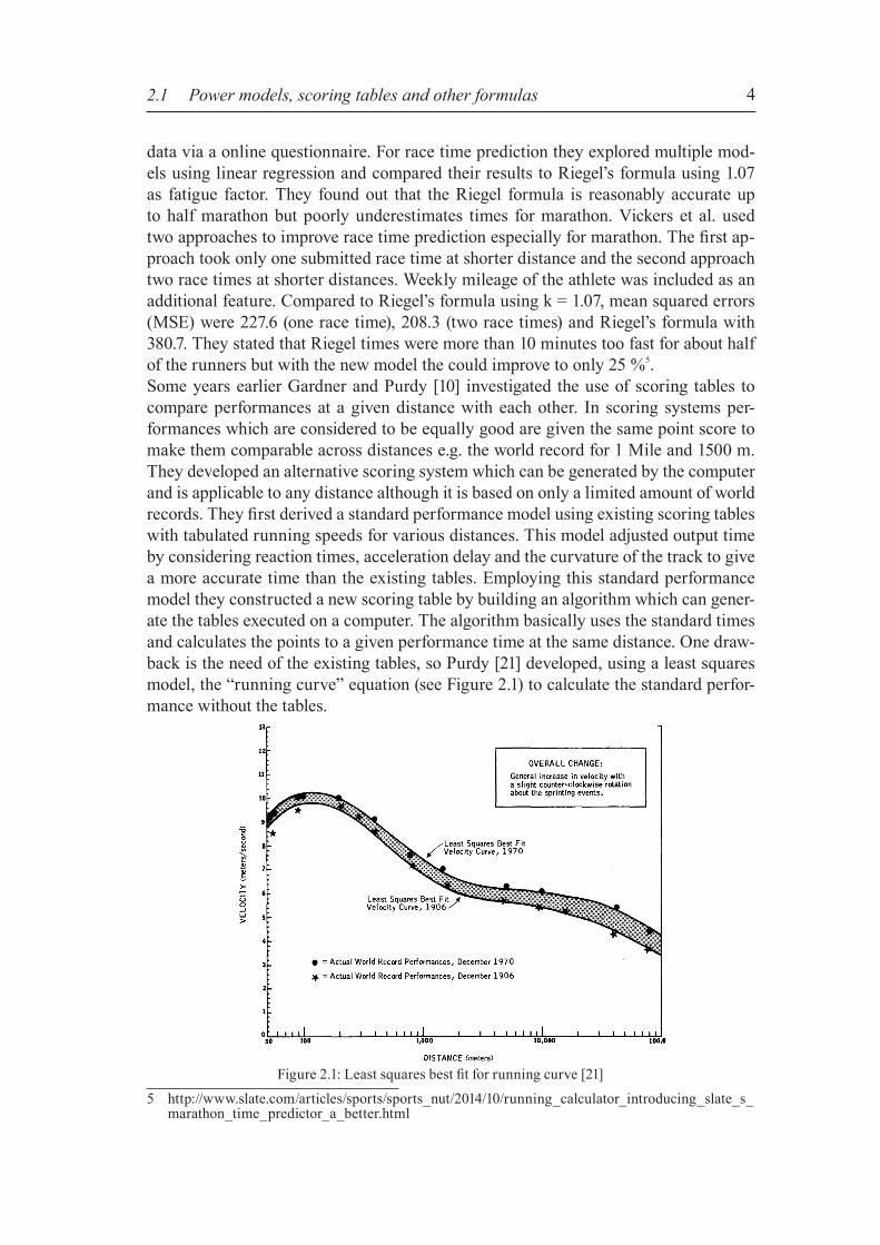
data via a online questionnaire. For race time prediction they explored multiple mod-els using linear regression and compared their results to Riegel’s formula using 1.07 as fatigue factor. They found out that the Riegel formula is reasonably accurate up to half marathon but poorly underestimates times for marathon. Vickers et al. used two approaches to improve race time prediction especially for marathon. The first ap-proach took only one submitted race time at shorter distance and the second approach two race times at shorter distances. Weekly mileage of the athlete was included as an additional feature. Compared to Riegel’s formula using k = 1.07, mean squared errors (MSE) were 227.6 (one race time), 208.3 (two race times) and Riegel’s formula with 380.7. They stated that Riegel times were more than 10 minutes too fast for about half of the runners but with the new model the could improve to only 25 %5.Some years earlier Gardner and Purdy [10] investigated the use of scoring tables to compare performances at a given distance with each other. In scoring systems per-formances which are considered to be equally good are given the same point score to make them comparable across distances e.g. the world record for 1 Mile and 1500 m. They developed an alternative scoring system which can be generated by the computer and is applicable to any distance although it is based on only a limited amount of world records. They first derived a standard performance model using existing scoring tables with tabulated running speeds for various distances. This model adjusted output time by considering reaction times, acceleration delay and the curvature of the track to give a more accurate time than the existing tables. Employing this standard performance model they constructed a new scoring table by building an algorithm which can gener-ate the tables executed on a computer. The algorithm basically uses the standard times and calculates the points to a given performance time at the same distance. One draw-back is the need of the existing tables, so Purdy [21] developed, using a least squares model, the “running curve” equation (see Figure 2.1) to calculate the standard perfor-mance without the tables.

5 http://www.slate.com/articles/sports/sports_nut/2014/10/running_calculator_introducing_slate_s_marathon_time_predictor_a_better.html

Figure 2.1: Least squares best fit for running curve [21]

2.1 Power models, scoring tables and other formulas

5

Purdy [10] and Riegel [22] used as reference data official world records which were set on completely flat tracks. Vickers [28] improved race time prediction for marathon especially for recreational runners but also for courses without elevation gain. James Elliott [8] did some analysis on marathon pacing and elevation changes taking into account the energy costs of running uphill and downhill. His analysis is based on observations how the pace of marathon runners changes on significantly hilly courses and resulted in several approximations of the energy costs and a coarse estimate of target paces for hilly marathons. His work builds on research by Myers and Higdon [13] where they analyzed pace changes in marathon on flat courses and described that the variations in the average pace can be broken up into 4 regions (12, 18, 23 miles). Very interestingly they found the same patterns of the 4 different pacing regions to be true for non-elite marathoners. Elliott used the findings of Myers and Higdon on flat courses and adjusted the paces for every mile by the energy costs for ascent or descent. Evaluation was done on the elevation profile of the Oakland Marathon and race results from 2012. His predictions for faster finishers were better than those for slower runners however his equation described the splits more accurately than Mayers and Higdon. Minetti et al. [20] investigated energy costs for running at extreme slopes and came up with an energy cost function for gradients up to ± 0.45. They stated, when running on positive gradients starting at 0.15 the energy cost increases as a function of the gradi-ent incline and when running on negative gradients lower than -0.15 energy costs are negatively related to the slope. Townshend et al. [27] published a paper about pacing over undulating terrain. They investigated limiting factors of running uphill and best strategies to optimize overall time while running over undulating terrain e.g. they suggest running slightly slower uphill to return faster to your normal pace on level because this is where their subjects lost time. Using multiple regression they also were able to predict speed from gradient data. Taking into account the influence of preceding climb sections using a decay func-tion to weight the gradients improved their prediction model significantly.

2.1 Power models, scoring tables and other formulas

6

2.2 More complex models using individual historical parameters

Tanda [26] examined the relation between marathon performance time and training characteristics recorded over several weeks and found how weekly mileage and train-ing pace both highly correlate with the average marathon pace. Through multiple non-linear regression he determined an equation to compute the average pace for a mara-thon given weekly mileage and average training pace. The standard error of estimate (SEE) of the equation was 4 min. for all participants and dropped to only 3 min. 35 sec. for the subgroup with BMI (body mass index) < 23 kg/m2. A very similar approach to predict marathon performance of amateur runners on the basis of their training data was investigated by Ruiz-Mayo et al. [23], although they in-cluded a lot more parameters characterizing each training session. For the analysis they used data from the 2015 London and Boston marathon. Athletes with less than 3 work-outs per weeks on average were removed as well as distances over 50 km and workouts with unrealistic fast paces. The filtered data included ~ 35 000 workouts from ~ 1000 athletes. They extracted characterizing attributes for time periods of training and fed them into a machine learning model. Longest distance, total net elevation gain, fast-est pace are just a few. Validation was done using 10-fold cross-validation and yielded with the filtered data set a mean absolute error (MAE) of 555 seconds (~ 9 minutes). An improvement to 436.3 seconds (~ 7 minutes) gave an even further filtering out athletes who presumably had troubles during the race. Good results attained Jin [14] with pace prediction for a given route using only three features for each training session: elevation gain, distance and recent 10 k race time. With 5-fold cross-validation Jin reached a mean squared test error of 0.5517 minutes with a basic linear regression model. There is no specific explanation why the error is so small but a potential reason might be the training data. Only data from 4 athletes is used with a total of 447 samples. A data set with very similar athletes concerning performance would result in very precise predictions. Plus, predicted distances are not explicitly named therefore the good result cannot count as a measure for other works. Millett et al. [19] explored two methods to predict race times on historical race data: locally weighted linear regression with workout specific features and a Hidden Mar-kov Model (HMM) modelling the fitness states of the athletes. They did evaluation of the regression model using leave-one-out cross-validation and predicted a future race with the HMM. As comparison, Riegel’s formula was used as a baseline plus a real coach gave predictions on a subset of 16 athletes with knowledge of their prior race performances. The complete set of race data consisted of 103 athletes all with 20 - 40 races in their history including track and cross-country races. Locally weighted linear regression yielded an overall error of 3.9 % (1.5 % on track races only) but failed to give any useful prediction for 10 % of all races. The HMM reached a slightly better re-sult with 3.8 % error. Surprisingly, the baseline had only an error of 4.1 % which is not much worse than the HMM with the best result. Since the coach did only predictions on a subset, the error rates cannot be compared directly but she achieved an error rate of 9.73 % and beat the baseline which got 11.71 %. Like Millett et al. [19] stated, the prediction models did not perform as well as expected but could beat the baseline. Still the HMM looks promising because it can model states of fitness very well.

2.2 More complex models using individual historical parameters

7

A completely novel approach presented Blythe et al. [3] reaching an average prediction error on elite marathon performances of 3.6 min. and 30 % improvement in root mean squared error (RMSE) over a range of distances compared to state-of-the-art predic-tors. They explained their improvement with the individualization of the power-law used in standard approaches. They discovered that three parameters represent an ath-lete: his endurance, his relative balance between speed and endurance and his special-ization over middle distances. Using an individual power-law and these three values allowed them to describe individual performances with a remarkably high precision. The underlying method used was Local Matrix Completion (LMC), a machine learn-ing technique to fill in missing entries of a partially observed matrix [4]. More than 150,000 athletes with ~ 1,400,000 performances formed the data set for analysis and evaluation. Since male and female runner performances were differently distributed, all results relate to the subset of ~ 100,000 male runners. Evaluation was done by leave-one-out validation for 1000 single performances omitted randomly. Smyth et al. [2] did research on recommender systems, which is not directly related to race time prediction but strongly correlates to finding the best pacing strategy. They explored a data set of 600,000 finish times and analyzed the differences between ama-teur and elite athletes. For example, they found out that amateur runners tend to run their best marathon performance some years later than elite runners since their first marathon and that elite runners peak at much younger ages than amateur runners. By going through the data of training plans, athletes with similar histories can get sug-gest training plans that are suitable for them and allow them to make huge progress in short time. Their prediction models k-nearest neighbors (KNN) and extreme gradient boosting (XGB) outperformed Riegel’s formula for amateur runners with error rates of 10.45 % (KNN) and 9.04 % (XGB), while Riegel yielded 12.8 % error rate. For elite runners (< 190 minutes) Riegel performed much better than KNN and XGB. The find-ings emphasize the notion that the knowledge of elite athletes can lead to a significant advantage regarding performance improvement. Going one step further, Smyth and Cunningham [24,25] presented a very specific ap-proach on how to build a recommender system that can be used in a marathon and will lead in the optimal case to a new personal best. While most runners know pacing strategies like even, positive or negative splits they argued that these strategies are much too coarse and suggested a finer splitting e.g. by segments of a certain length or by hills. A precondition for using their recommender system is one finished marathon at exactly the same or very similar course with a suboptimal time or non personal-best (PB). The used method to recommend pacing plans was Case-based reasoning (CBR) which tries to solve new problems by reusing and adapting similar past problems [15]. For generating a new plan they identified k runners who finished the given marathon multiple times with a non PB similar to the query runner and a faster PB on the same course. They argued, since it was possible for the similar runners to achieve a new PB after running the query runner’s time the years before, then a similar new PB should be achievable by the query runner. Evaluation was done on data from the Chicago marathon [24] and the London marathon [25] resulting in ~ 100,000 cases for the for-mer and ~ 13,000 for the latter. As a measure of accuracy the percentage error between predicted PB and actual PB was calculated. As a measure of pacing profile similarity the relative differences between the segment paces of the recommended plan and the

2.2 More complex models using individual historical parameters

8

actual pacing profile were computed. They achieved errors of 4 - 5 % (female 4 %) on average and race plan similarities of more than 90 %. Like they stated, faster runners may be more predictable as the error starts at 2.5 % for 180-minutes marathoners and increases to 5 % after the 300 minutes mark. But more important for the recommender system, they showed that e.g. a 4-h marathoner can improve his non PB by ~ 20 min-utes to a new PB (see Figure 2.2). Smyth and Cunningham [24,25] presented a novel approach in race time prediction and even went one step further in recommending a pacing plan to achieve a new personal best. What has to be kept in mind that this ap-proach still needs the proper training to run a new record, it just shows how athletes performances can be compared and how appropriate pacing strategies can be found and proposed for query athletes.

2.3 Comparison to our approachIn the following we look again at the presented related work to find possible advan-tages or disadvantages and compare it to our approach to show similarities and where we can improve. First we presented approaches using power models, scoring tables or other formulas that were partly developed more than 40 years ago but are still valid and commonly used. These approaches are easy to use as they result most of the time in a formula that requires only a few parameters. Riegel [22] for example fitted a power model that just needs an recent record of a race and the predicting distance. Purdy et al. [10,21] used scoring tables to compare performances over different dis-tances but developed an algorithm that also needs the variables mentioned above. Vick-ers et al. [28] who added a second record of a race and weekly mileage to his model to improve Riegel’s marathon predictions got credited by Runner’s World Magazine. Elliott [8] investigated the inclusion of elevation changes during a marathon into the predictions. Every runner knows that elevation change has a huge impact on the aver-

Figure 2.2: Predicted PB improvements based on non PB times [25]

2.2 More complex models using individual historical parameters

9

age pace of race and needs to be included in predictions. Minetti et al. [20] and Town-shend et al. [27] showed how to compute energy costs of running up- or downhill and how to account for elevation changes while running a hilly race. Riegel’s or Purdy’s predictions can not be used for races with any significant elevation changes since they rely on race times set on flat courses. Asking one of the available predictors that use one of these formulas or built upon them to predict a finish time for a trail or any other hilly race would presumably result in an overestimation of the performance time. An other aspect that applies to Riegel and Purdy is that the models are based on world record times set by world class athletes in perfect situations. The goal was to find relationships between distance and time that describe the human ca-pabilities in running. It is a best fit for a set of very optimal times but does not take into account individual variance to that best fit. It can be seen that adding more information about an athlete improves the prediction for marathon [26].In the second part we investigated approaches that rely more on the individual athlete and what he achieved in training up to the attempt of Millett et al. [19] to model an athletes fitness and use it for predictions. At the end we presented the work of Smyth et al. [24,25] and how a recommender system could predict a pacing plan to achieve a new personal record. In their research they do not only predict a race time but look at smaller segments of the course and propose a strategy how to reach a better race time. This approach compares the athlete’s performance with similar performances of other athletes and does the prediction on their achievements. Since Smyth et al. [24,25] did no actual evaluation using their recommender system in action it is not clear how their approach performs in reality. But what is clear is the fact that proper training (maybe similar training) is needed to guarantee a new personal best. A drawback of their ap-proach is the requirement of a finished marathon on the same course. Nevertheless, looking at our initial idea for the thesis of finding the optimal pacing strategy for a given race, this approach is highly related to our idea. Comparing the presented works to our approach, we would be introduced in the second subchapter with works that look at the individual athlete. Our approach results not in an easy to use formula but in a neural network that can predict times for any distance. Like Blythe et al. [3] we want to analyze the individual training data and extract fea-tures that describe the athlete’s fitness, capabilities to run on hills and his state of fa-tigue. Our second approach is comparable to Elliott’s [8] method. We also do not look at a workout as a whole but divide it in segments based on the profile of the course to explicitly predict times for segments with a certain gradient. Some of the works just focused on one distance e.g. marathon, but we want to cover any given distance. The main drawback in our approach compared to Riegel or Purdy is that we possible can-not predict very well for distances that we have not seen so far. Riegel’s formula for example knows how the average pace decreases with increasing total distance based on data from other athletes. In our approach, we only look at the individual athlete and if we have only seen 5 k performances it is more likely to give an inaccurate prediction for a marathon time. Nevertheless, since Riegel’s formula is still a standard way to predict race times even it got improved by Vickers et al. [28], we will use it as a baseline in the evaluation part of the final study to compare our results and to have a relative measure of improvement.

2.3 Comparison to our approach

10

3 Survey

In order to get an initial understanding of race preparation of runners, we conducted an online questionnaire. The questionnaire was conducted to get an early feedback from active runners and get inspired by their experiences. Additionally, the survey included data acquisition for evaluation of the models.

3.1 Overview of the questionnaireSince in this survey we are targeting Strava users, we opted for a online questionnaire, in our case Google Forms. Overall, the questionnaire consisted of 24 questions (17 mandatory) split in three parts: demographic questions, running habits related ques-tions and pacing strategy related questions. Some questions were multiple choice with just one answer, others with multiple answers and a few open text answers. A German and a English version of the questionnaire was used to not only get feedback from one country but a vast variety of cultures. We distributed the link to the questionnaire via various running related Facebook groups and posted in local and international Strava groups. Addressed athletes also included triathlon and duathlon athletes.

3.1.1 Participants

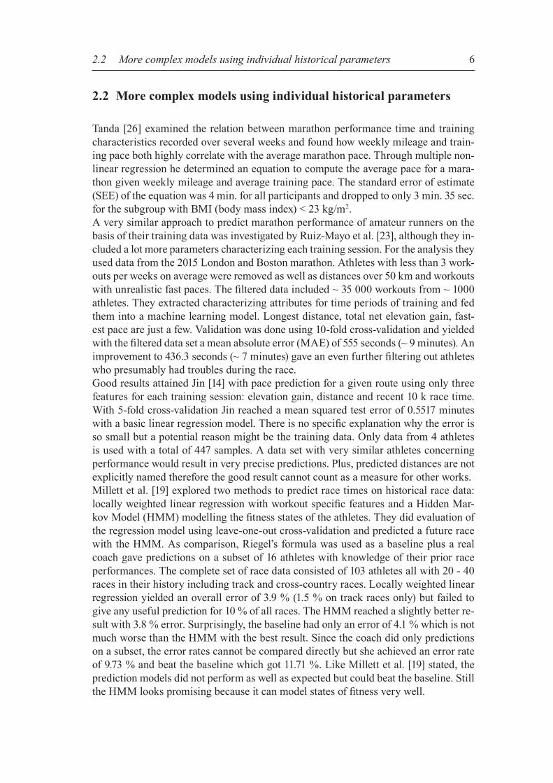
The first part consisted only of demographic questions like gender, age or country. Overall 330 people (253 male, 77 female) submitted their answers. Since we also ad-dressed English speaking people we got answers from more than 20 countries. Most of the participants came from Germany (64.7 %) followed by the USA (14.5 %). Bel-gium (4.4 %), Switzerland (4.1 %), Netherlands (3.5 %) and UK (2.2 %) follow with diminishing percentages, while the rest countries account for less than 7 % in total. The country distribution is heavily influenced by the choice of Strava and Facebook groups. Figure 3.1 shows the age group distribution. The main part of the participants is over 20 years and under 55.

Figure 3.1: Age group distribution of the participants (330 answers)

11

3.1.2 Running expertise

In the second part we asked running related questions to get an overview of the capa-bilities of the individual athlete. These questions were also crucial to find our target group. Asking for runs per week and weekly mileage gives us an indication how long a runner has been running, provided that the answers are not biased by the feeling of the runner. Beginners usually start with a low mileage and increase the amount of workload with more years of running. Regarding races, we asked how many races the athlete finished successfully, which kind of races and what the personal records are. There exist many kind of races in long distance running, from 5 k up to marathon and even ultra marathon. Besides distance, there exist differences in the underground like track, road, cross country and trail running. Another big group that needs to be included are triathletes or duathletes. Knowing these characteristics of running expertise, we can coarsely group and classify the participants. They also had the chance to give a self-assessment including personal records for 5 k, 10 k, half marathon and marathon. There exists no strict classification in literature for the level of a long distance runner, so we took the most often used in online articles, namely “recreational runner (for relaxation)“, “ambitious recreational runner“, “competitive runner“ and “professional runner”. The last questions in the running related part explored, how the athletes prepare for races, if they get help from a coach or very experienced running buddy, how often they follow prepared plans and what the problems are while preparing and following a plan. These questions reflect what crucial elements in race preparation are, if there is knowledge and experience behind it and which problems can occur due to misplan-ning. A goal for the strategy predictor was to make manual planning obsolete and help the athlete to follow the strategy without running into problems.

3.1.3 Pacing strategies and race time predictors

The last part of the questionnaire addressed pacing strategy related questions and in-troduced the idea of a pacing strategy predictor. A hypothesis we made before is, that current predictors only take into account a few parameters but performance is often af-fected by more than old personal bests. First, we asked if the athlete has ever used any calculator or other tool to predict times for a race and asked about his opinion of the quality of the predictions. Further, the participants got a brief description of the idea behind a pacing strategy predictor followed by a few questions. Due to the hypothesis we made, we asked what parameters influence the athletes’ performance on race day and should be taken into account in a predictor. The most important questions were, if one would benefit from such a predictor application and the likeliness of usage.Optionally, all participants could grant access to their Strava training data after they finished all questions. These data was used to develop the predictor model and served for the technical evaluation of the models.

3.1 Overview of the questionnaire

12

3.2 Results

In the following section we will review and analyze the most important and meaning-ful answers. Participants were asked, how many runs on average they do and how high their weekly mileage is. Both questions were single choice questions and the answers are illustrated in Figure 3.2. The majority runs 3 - 4 times a week (56.7 %) followed by 5 - 7 times (29.4 %). 11.8 % participants run just 1 - 2 times per week and can be con-sidered as recreational runners with little ambition to improve running performance. A few athletes stated (1.5 %) that they do double runs and it can be assumed that they belong to the professionals or very competitive runners. At the same time we find 1.5 % athletes running more than 110 km on average every week, which corresponds to running more than 7 times per week. Still at a very high level, 4.5 % of all participants accumulate 90 - 110 km per week and 11.5 % reach 75 - 89 km. More than a third has a mileage of over 50 km and can be considered as runners with experience. Both, runs per week and weekly mileage contain some information about the level and experience of a runner. Mostly, new runners start off slowly and increase their mileage with the years once their body adapted to the workload. Figure 3.2 indicates that at least one third of the participants are experienced runners and approximately an other third are no beginners and can handle a fair amount of mileage per week.

Figure 3.2: Runs per week (330 answers) and weekly mileage (330 answers)

3.2 Results

13

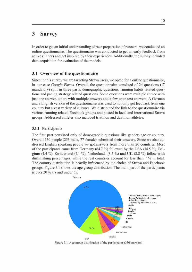
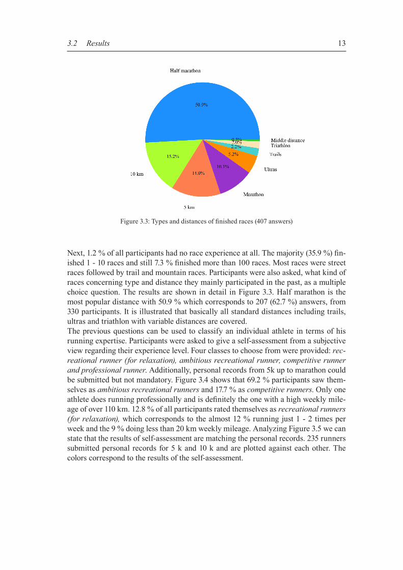
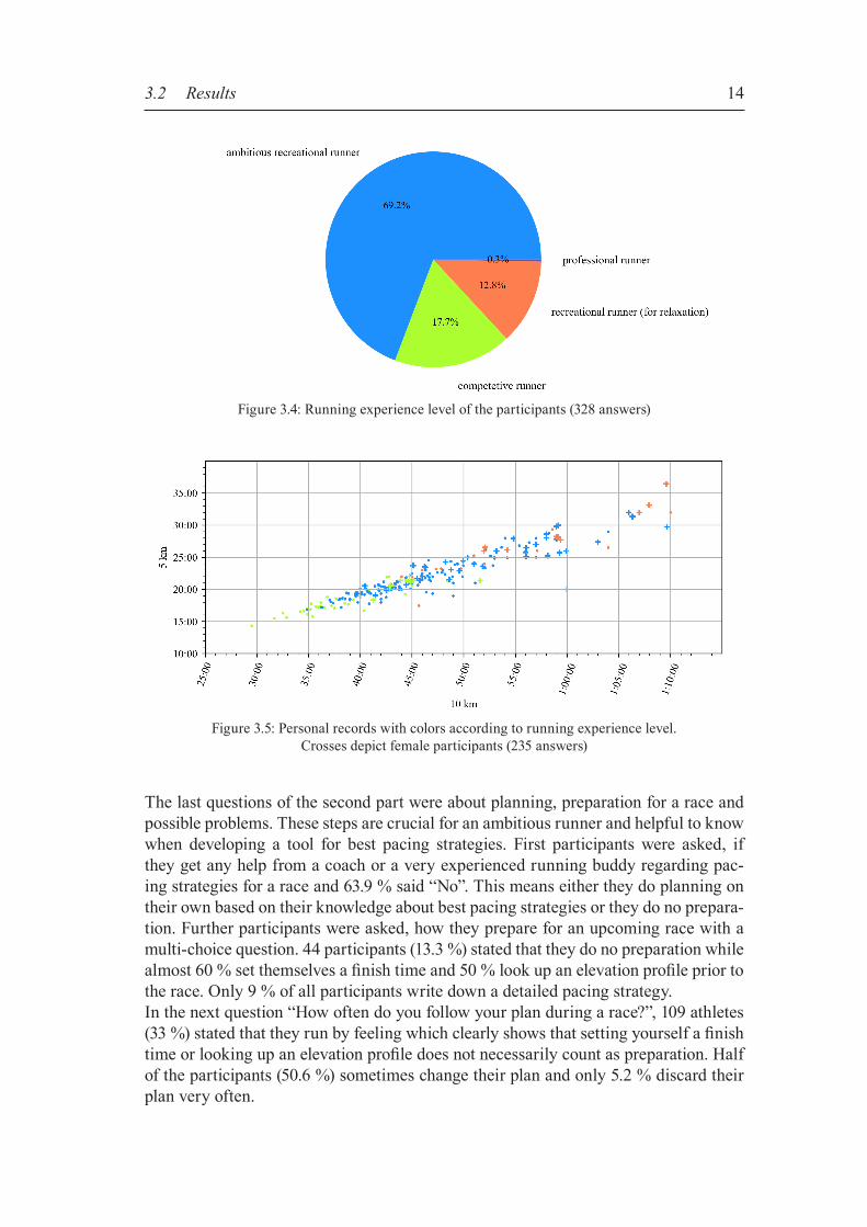
Next, 1.2 % of all participants had no race experience at all. The majority (35.9 %) fin-ished 1 - 10 races and still 7.3 % finished more than 100 races. Most races were street races followed by trail and mountain races. Participants were also asked, what kind of races concerning type and distance they mainly participated in the past, as a multiple choice question. The results are shown in detail in Figure 3.3. Half marathon is the most popular distance with 50.9 % which corresponds to 207 (62.7 %) answers, from 330 participants. It is illustrated that basically all standard distances including trails, ultras and triathlon with variable distances are covered. The previous questions can be used to classify an individual athlete in terms of his running expertise. Participants were asked to give a self-assessment from a subjective view regarding their experience level. Four classes to choose from were provided: rec-reational runner (for relaxation), ambitious recreational runner, competitive runner and professional runner. Additionally, personal records from 5k up to marathon could be submitted but not mandatory. Figure 3.4 shows that 69.2 % participants saw them-selves as ambitious recreational runners and 17.7 % as competitive runners. Only one athlete does running professionally and is definitely the one with a high weekly mile-age of over 110 km. 12.8 % of all participants rated themselves as recreational runners (for relaxation), which corresponds to the almost 12 % running just 1 - 2 times per week and the 9 % doing less than 20 km weekly mileage. Analyzing Figure 3.5 we can state that the results of self-assessment are matching the personal records. 235 runners submitted personal records for 5 k and 10 k and are plotted against each other. The colors correspond to the results of the self-assessment.

Figure 3.3: Types and distances of finished races (407 answers)

3.2 Results

14

The last questions of the second part were about planning, preparation for a race and possible problems. These steps are crucial for an ambitious runner and helpful to know when developing a tool for best pacing strategies. First participants were asked, if they get any help from a coach or a very experienced running buddy regarding pac-ing strategies for a race and 63.9 % said “No”. This means either they do planning on their own based on their knowledge about best pacing strategies or they do no prepara-tion. Further participants were asked, how they prepare for an upcoming race with a multi-choice question. 44 participants (13.3 %) stated that they do no preparation while almost 60 % set themselves a finish time and 50 % look up an elevation profile prior to the race. Only 9 % of all participants write down a detailed pacing strategy. In the next question “How often do you follow your plan during a race?”, 109 athletes (33 %) stated that they run by feeling which clearly shows that setting yourself a finish time or looking up an elevation profile does not necessarily count as preparation. Half of the participants (50.6 %) sometimes change their plan and only 5.2 % discard their plan very often.

Figure 3.5: Personal records with colors according to running experience level. Crosses depict female participants (235 answers)

3.2 Results

Figure 3.4: Running experience level of the participants (328 answers)

15

The last question asked for the problems by creating a plan and following it during a race. This was a multi-choice question with 416 total answers illustrated in Figure 3.6. The main reason why failing or getting into trouble was a too fast start resulting in early fatigue (148 answers). Almost a third of all participants (107 answers) have no problems during a race. Finding an elevation profile nowadays or forgetting parts of a prepared plan appears not to be a problem, while overestimation of the own maximal performance is the second reason for failing (86 answers). “Others” abstracts problems added by the participants including underestimation of the own capabilities, external factors like weather conditions, or the form of the day.Those, who run by feeling basically have the same problems like the rest and of those, who always follow their plan, almost 50 % have problems. Even the ones who get ad-vice from a coach have the same problem patterns. This let us conclude, that we cannot gain much information what the reasons for problems are, but most runners experience them although they might not be severe.In the last part of the questionnaire participants were asked questions related to the idea of a pacing strategy predictor. First they were asked if they have ever used an ap-plication or tool that predicts their finish time for a race or calculates splits. In an open text question they could submit their opinion about the quality of the predictions. 58.8 % of the participants have already used a predictor and roughly 57 % gave feed-back about the quality. Different opinions were submitted: ~50 % can be classified as negative and ~15 % had no strong opinion. Only about ~35 % answers were positive and rated the received predictions as helpful. The mostly named negative comments referred to inaccuracy, too pessimistic or optimistic predictions, too many factors like elevation, weather, fitness etc. are not included in the calculation, and that they are designed for perfect situations and not the real world.

Figure 3.6: Overview of problems before and during a race (416 answers)

3.2 Results

16

Next, an imaginary application that employs the idea of a pacing strategy predictor got introduced in a few sentences. The participants were informed that the applica-tion would use their Strava data, process it automatically to a race plan that can be displayed on a running watch during a race and in the best case would help to achieve a better time. Like already mentioned, current predictors take into account only a few parameters like last personal best or weekly mileage therefore we asked in a multiple choice ques-tion what parameters do influence the performance on race day and should be taken into account in the imaginary application. Few answer choices were given but peo-ple added own answers. The most voted factor that affect people’s performance was weather (73.6 %) which is clearly the most uncontrollable variable. As some athletes like cold temperatures more than others, racing in the heat strikes almost every run-ner and significantly declines the performance level. Very close together were sleeping quality before a race (47.9 %), personal motivation (45.5 %) and the start time of the race (41.2 %). Minor injuries only affected 21.8 % which could come from the fact that most runners only race when feeling fit. By the participants added factors were nutrition / fuel with 5.2 % followed by tapering / fatigue, form of the day, competitors among the contestants and the journey to the race all with diminishing percentages. The last two questions of the questionnaire were designed to find out, how much the participants think, they would benefit from using the application during a race and how likely they would use it if it was available. Figure 3.7 shows the four possible answers and how the participants voted. 63.4 % of the answers are positive with 57.3 % saying that they would benefit. The rest is more than positive about the benefits of the applica-tion. Only 7.6 % do not see any value or use in it and almost a third (29.1 %) think they would not benefit. Additionally, Figure 3.8 shows the distribution of the likeliness that the participants would use the application. They could rate from 1 to 10 with 1 meaning very unlikely and 10 meaning very likely. Figure 3.8 indicates that most of the ratings are on the right side towards the 10. Numbers with the most answers are 8 (20 %) and 7 (19.4 %) which lies between very likely and neutral, slightly more neutral. The number with the fewest ratings are 1 (5.2 %) and 2 (5.5 %). Looking only at positive and nega-tive ratings split evenly in the middle, there are 62.8 % positive ratings. 88.4 % of those who rated positively, think that they would benefit from using the application and only 11.6 % see no benefit. 21.1 % of those who rated negatively said before that they would benefit. This discrepancy might be caused by the fact that more than 20 % voted a 5 or a 6 which is quite neutral although they think they could benefit or not.

3.2 Results

17

At the end every participant optionally had the chance to write down ideas and critique related to the idea of the pacing strategy predictor as a feedback for us. Very useful and inspiring ideas were submitted but the answers will not be discussed here in detail. An overall feeling concerning ideas and acceptance, it can be stated that athletes from other countries were more open and enthusiastic about the idea and left some very use-ful remarks while German participants were quite restrained and neutral.

Figure 3.8: Distribution of likeliness to use the application (330 answers)

3.2 Results

Figure 3.7: Illustration of how many see a benefit in the application (330 answers)

18

3.3 DiscussionIn the following section we will summarize our findings described above and complete the chapter with extracting relevant and helpful information in terms of target group and weaknesses in current predictors to motivate our work. Participants covered all age groups, different countries and almost a quarter female athletes participated. Participants had experience at all standard distances, having more or less experience in running races and the majority rated themselves as ambi-tious recreational runners. Most participants invest some time for preparation before a race but half of the athletes changes their plan sometimes due to problems like starting too fast or overestimation of the own capabilities. At the end, participants were more positively minded than sceptical and almost two third considered the proposed applica-tion as beneficial while ~60 % would eventually use it.The main goals of the questionnaire were to find out who the target group is and to find out what is missing in current predictors in the eyes of the participants. To define the target group we started by selecting all participants who would most likely use the application. To make it more clear, we filtered for those who rated a likeliness of 6 or higher and got 177 (53.6 %) participants. More than 92 % of them think they would also benefit, what makes them more to a long time user providing proof that they benefit of it. They basically do the same preparation like all others, but slightly fewer have no problems during a race (27.1 % compared to 32.4 % including all). 64.4 % of the selected group have already used a prediction tool or calculator before and may know about limits and weaknesses. Racing experience and race types show no significant differences compared to the whole participant set, but what is more important how they rated themselves in the self-assessment. Nearly three quarter of them (74.6 %) classi-fied themselves as ambitious recreational runners, 14.7 % as competitive runners and 10.7 % as recreational runners (for relaxation). The conclusion we can make is that the better an athletes gets and the more professional he runs, the more he trust his own or his coaches experience and do not need help from “assistive” tools. For the relaxation class, one can conclude that their motivation for running is not mainly competition driven and they are not so much interested in supportive technologies. Concerning gender or age group, we can not identify significant differences to all other athletes.To sum it all up, the main target group are ambitious recreational runners who can imagine to benefit using the application. They do preparation for races but sometimes change their plans during races due to problems like starting too fast or overestimating themselves. Most of them already used current prediction tools or similar applications and while some are happy with the results others criticize the quality. Most mentioned critique is that too less factors are taken into account and the predictions are to general and designed for perfect situations all at the cost of loosing individuality.What we can take out of the questionnaire is, that adding elevation gain as an ad-ditional factor for race time prediction and also taking into account extensively more historical information than current predictors, should give us an advantage and in a best-case scenario significantly better results.

3.3 Discussion

19

4 Implementation

In this chapter, two approaches on how to predict race time on historical training data are presented in detail. A working prototype consisting of two separate parts was im-plemented – first, a server based application to collect the training data and compute the features, and second, classes containing the neural network and its evaluation. In the following, we first describe how we collected and processed the historical training data. Subsequently, the structure of the neural network and its function as a regression model gets explained. Then, the two approaches get presented including pre-analysis, computation of the features, training of the neural network and evaluation. For the evaluation of both models, training data obtained from participants of the survey get used to quantify the quality of the models using cross-validation. Figure 4.1 shows a high-level architecture illustration of the system and how the original training data gets processed step by step.

Figure 4.1: High-level architecture illustration of the system

20

4.1 Historical training data After Garmin released its first GPS running watch in 20036, people started more exten-sively to track their training in GPS coordinates. New options in logging and analyzing training opened up for recreational runners. As research improved the GPS accuracy and battery life, running watches became more usable and are nowadays an ubiquitous addition in running. Tracked activities can be uploaded to websites designed for ana-lyzing and visualizing workout efforts. Strava is such an website and the source of all training data used in the thesis.For us very important is a powerful API to get access to the athlete‘s history in the form of GPS data. Strava provides a well documented API7 with a free limited access of 30,000 requests per day. The activity history of an athlete can be accessed via the API once the athlete granted permission. Basically, all parameters saved by the track-ing device are available, plus some extras computed by Strava after the upload. Mass raw data like GPS coordinates, elevation data or velocity can be accessed via so called “streams”, an array-like structure with one entry per tracked point. Data can be accessed with an access token received during the authentication pro-cess. Strava uses OAuth28 as an authentication protocol to allow external applications to request authorization to a user’s private data without the need of user name and password. OAuth2 is a standard protocol to handle authorization processes and keep the login credentials save. The Strava API v3 requires HTTP requests that need to be implemented in a safe way to query data. Open source libraries doing the requests have been implemented in various languages by the community and are listed in the API documentation. We used the Strava API REST client “StravaPHP”9 that provides PHP methods to access the API and includes authorization and authentication steps for easy integration in a new application. We built a web server based application accessible via the browser to download the activities from Strava and to save all needed values in a database on the server. From there we could write the features for training of the neural network to files and do the training offline. All server related functionality is written in PHP and all neural net-work related code is written in Python. Python is widely-used in machine learning.In the following sections, basic parameters and concepts get described that will be needed as features for training the models of the two approaches to predict race times.

6 https://www.runnersworld.com/gps-watches7 https://strava.github.io/api/8 https://oauth.net/2/9 https://github.com/basvandorst/StravaPHP/

4.1 Historical training data

21

4.1.1 Elevation data

Elevation data recorded by modern running watches is still a problem, particularly when calculated by the GPS signal10,11. Watches with barometric altimeters provide a slightly better precision but the values can still be off due to weather changes12. Not every running watch uses a barometric altimeter, only more expensive models. This means that to compute a correct value for the elevation gain, the raw altitude data needs to be corrected. Strava does elevation correction for activities recorded on de-vices without barometric altimeter. They built an elevation look-up service powered by data from the Strava community and uses it as a database to update the elevation data during correction15. This method heavily relies on the accuracy of devices barometric altimeters. Tests on a for us well known course, that is frequently used by several athletes who upload their activities to Strava, was examined with focus on the quality of the eleva-tion data corrected by Strava and provided via the API. We found significant errors in the elevation profile what resulted in an overestimated elevation gain and a visual discrepancy of the profile (see Figure 4.2), even after smoothing. Since the course is located around a hill some steep segments are part of the recorded activities. Severe errors were found, e.g. the profile showed a longer downhill section followed by an impossible positive slope within a few meters where is in reality only a longer uphill section. We believe that sometimes false elevation values caused by faulty GPS signals or inaccurate barometric measurements get saved into the basemap of Strava. We compared Strava data to other elevation profiles plotted with elevation data from Open Street Map13 (OSM) and Google Elevation API and found Google Elevation API giving the best results (Figure 4.2). Google uses different sources, thus can provide a better resolution than OSM or Strava. The Google Elevation API has free limited ac-cess, is easy to use and we found while testing for some areas a resolution better than 20 m14. Although using a different service to determine the altitude data is cumber-some, we decided for Google Elevation API because our approaches rely on the ac-curacy of elevation data.

10 http://geoawesomeness.com/accurate-altimeter-gps-watch/11 https://support.garmin.com/faqSearch/en-GB/faq/content/QPc5x3ZFUv1QyoxITW2vZ612 https://support.strava.com/hc/en-us/articles/216919447-Elevation-for-Your-Activity13 https://www.openstreetmap.de/14 https://developers.google.com/maps/documentation/elevation/intro

Figure 4.2: Differences of the elevation profiles obtained from Strava and Google

4.1 Historical training data

22

An other factor that affects the accuracy of the elevation data is the GPS signal. Run-ning watches are only to a certain extend accurate and cannot be used to display the real running pace15. Errors to all orientations can occur, which affect the running pace or put the GPS coordinates off the track. Wrong coordinates implicate false elevation data, even if the altitude measurements are correct. Therefore, there are two factors that manipulate the accuracy of the elevation data: the GPS signal and the elevation data source.A first step to remove some of the errors is smoothing the data. The GPS data is al-ready more or less smoothed by the device and Strava, so we used the raw coordinate stream from Strava. On every coordinate of that stream we queried the Google Eleva-tion API to get the altitude of that point. The received values produce a very jittery elevation profile plot like shown in Figure 4.3. The Ramer-Douglas-Peucker (RDP) algorithm is an iterative method to take a curve composed of connected points and find a similar curve with fewer points, a simplified curve [7]. The resulted points are a subset of the original points found by removing successively points that are “too far away“ from most of the other points. With this method noisy outliers can be removed, plus the total number of points gets reduced resulting in a coarse representation of the original [16]. The upper plot of Figure 4.3 shows the original noisy values and the simplified result after applying the RDP algo-rithm. One can see that the plot still contains lots of ups and downs which would result in a highly overestimated elevation gain. In the real world usually there are not so many changes in altitude within a small distance – the terrain changes smoothly. In the second approach, we split the whole activity in smaller segments based on the gradient of the course, therefore we can use these segments also to get a coarser representation of the elevation profile. How we computed the segments in detail, will be described later but the result is shown in the lower plot of Figure 4.3.

15 http://fellrnr.com/wiki/GPS_Accuracy

Figure 4.3: Smoothing of the elevation profile using RDP and segment algorithm

4.1 Historical training data

23

Given the segments, a good approximation of the elevation gain can be computed, which is the positive gain of altitude per segment added up to a total gain. Elevation gain does not tell much about how an elevation profile looks like, it is just the sum of sections with a positive gradient. A route with an elevation gain of 100 m could be very flat with just one climb somewhere in between or it could be undulated with a lot of very smooth hills. The percentage hilliness of a course gives more information about the profile. All segments with a positive or negative gradient starting at a certain threshold count as hilly and get set into relation to the flat parts. A route with 100 m elevation gain and 20 % hilliness is most certainly quite flat with just a few steeper climbs.The “FIETS Index” is a measure for the hardness of a climb developed by the dutch cycling magazine “FIETS”16. Although originally developed for cycling, it can be used for running as well. The running portal “Runalyze” employed the FIETS index in a new climb ranking measurement for running, the climb score17. The climb score values an activity between 0.0 and 10.0 regarding to the hilliness, the length and the overall demands of the climbs. Inspired by Runalyze, we incorporated the climb score as an additional representation of the elevation profile of an activity. Given the segments, it is trivial to find the climbs for the calculation of the climb score. All segments above a certain gradient and a reasonable length count as climb while short downhill sections do not interrupt a climb. Figure 4.4 illustrates the climbs found in the same elevation profile like in Figure 4.3.

16 https://www.pjammcyclingus.com/fiets---standard.html17 https://blog.runalyze.com/de/aenderungen/runalyze-v4-2-aenderungen/

Figure 4.4: Climbs found to calculate the FIETS index

4.1 Historical training data

24

4.1.2 VO2max

VO2max is a measurement of an athlete‘s aerobic capacity or in other words it is the maximum rate at which oxygen can be transported via blood to produce aerobic energy in the muscles. The units are milliliters of oxygen per kilogram body mass per minute (ml/kg/min)18. It is an indicator of endurance capacity as it reflects the ability of the heart to pump oxygenated blood efficiently to the working muscles. Several scientists have found correlation between VO2max and race performances. Daniels and Gilbert [6] published a formula in 1979, which approximates an athlete‘s VO2max. They used that formula to generate tables that predict a person‘s all-out rac-ing time for a given distance. Their work indicates that a higher VO2max is highly correlated with a better performance time. The formula divides the oxygen costs for a given velocity by the percentage of a person‘s maximum oxygen uptake needed for a given time, to estimate the VO2max19.

To account for elevation changes, we added the difference between two times elevation gain and one time elevation loss to the total activity distance before determining the velocity like suggested by Runalyze20. With this formula we could estimate people‘s VO2max for each activity and monitor how it changes over time.

4.1.3 Modeling human performance

Athletes train to improve their performance. Continuous training signals the body to adapt to the training impulse. But a very important part of all training is the recovery phase where the adaption takes place. So the main task for runners is to find a balance between training and recovery to most efficiently improve performance without risk-ing overtraining and injuries.

Impulse-response modelsTRIMP (training impulse) is a measure to model the training effect of an workout to the body. There exist several models incorporating TRIMP to optimize the relation between training stress and recovery over a longer period, also referred to as impulse-response models. One of these models is the so-called Training Stress Balance (TSB) model which is a simplification of a model proposed by Banister et al.21 in 1975, using an exponential decay to model the effects of training stress. The impulse-response models have positive and negative effects that need to be optimized to get an overall optimal outcome. In the TSB model the positive effect is the achieved fitness which is

18 https://www.runnersworld.com/vo2-max19 http://www.simpsonassociatesinc.com/runningmath2.htm20 https://help.runalyze.com/de/latest/calculations/vo2max.html21 https://www.trainingpeaks.com/blog/the-science-of-the-performance-manager/

4.1 Historical training data

25

called “Chronic Training Load” (CTL) and the negative effect is the accumulated fa-tigue termed “Acute Training Load” (ATL), resulting in the “Training Stress Balance”, the outcome performance22. In the TSB model, CTL and ATL are based on TRIMP which can be measured in different ways. The TRIMP of each workout forms the CTL and ATL, where CTL is the long-term effect of some training impulse and ATL gets only affected for a short time. Both are exponential moving averages over the TRIMPs, where CTL typically starts 42 days back and ATL 7 days. The overall goal is to maximize the TSB by training enough to increase the CTL while keeping ATL low before race day. TSB is just the difference between CTL and ATL and should not slip off too far below zero.We used the TSB model to represent the state of an athlete in terms of fitness and fa-tigue. When racing, tapering becomes a key aspect in the weeks before a race. If one goes into a race with pre-fatigue, most certainly it will affect the performance time. While some regenerate very quickly others need more time. Tapering and overall fit-ness can be modeled with TSB and gives us a good summary of an athlete’s recent training history. Figure 4.5 shows how a TSB model can be illustrated23.

22 http://fellrnr.com/wiki/Modeling_Human_Performance#cite_note-TSB-423 https://help.trainingpeaks.com/hc/en-us/articles/204071874-Performance-Management-Chart

4.1 Historical training data

Figure 4.5: Visualization of Training Stress Balance model

26

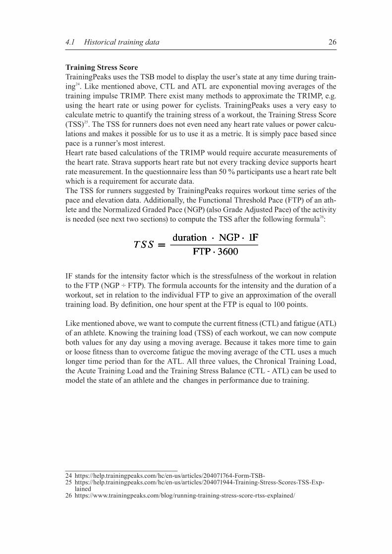
Training Stress ScoreTrainingPeaks uses the TSB model to display the user’s state at any time during train-ing24. Like mentioned above, CTL and ATL are exponential moving averages of the training impulse TRIMP. There exist many methods to approximate the TRIMP, e.g. using the heart rate or using power for cyclists. TrainingPeaks uses a very easy to calculate metric to quantify the training stress of a workout, the Training Stress Score (TSS)25. The TSS for runners does not even need any heart rate values or power calcu-lations and makes it possible for us to use it as a metric. It is simply pace based since pace is a runner’s most interest. Heart rate based calculations of the TRIMP would require accurate measurements of the heart rate. Strava supports heart rate but not every tracking device supports heart rate measurement. In the questionnaire less than 50 % participants use a heart rate belt which is a requirement for accurate data. The TSS for runners suggested by TrainingPeaks requires workout time series of the pace and elevation data. Additionally, the Functional Threshold Pace (FTP) of an ath-lete and the Normalized Graded Pace (NGP) (also Grade Adjusted Pace) of the activity is needed (see next two sections) to compute the TSS after the following formula26:

IF stands for the intensity factor which is the stressfulness of the workout in relation to the FTP (NGP ÷ FTP). The formula accounts for the intensity and the duration of a workout, set in relation to the individual FTP to give an approximation of the overall training load. By definition, one hour spent at the FTP is equal to 100 points.

Like mentioned above, we want to compute the current fitness (CTL) and fatigue (ATL) of an athlete. Knowing the training load (TSS) of each workout, we can now compute both values for any day using a moving average. Because it takes more time to gain or loose fitness than to overcome fatigue the moving average of the CTL uses a much longer time period than for the ATL. All three values, the Chronical Training Load, the Acute Training Load and the Training Stress Balance (CTL - ATL) can be used to model the state of an athlete and the changes in performance due to training.

24 https://help.trainingpeaks.com/hc/en-us/articles/204071764-Form-TSB-25 https://help.trainingpeaks.com/hc/en-us/articles/204071944-Training-Stress-Scores-TSS-Exp-

lained26 https://www.trainingpeaks.com/blog/running-training-stress-score-rtss-explained/

4.1 Historical training data

27

Functional Threshold PaceThe FTP is the average pace a runner can hold when running at an all-out effort for 45 - 60 minutes27. To determine this pace, different tests can be performed, but to do this automatically, the easiest way is to look at recent races and use e.g. Riegel‘s for-mula to compute a correspondent 60 minutes pace. Since we know the athletes‘ races, we searched for races within 6 month with the best performance. If this performances were between 45 and 60 minutes, we already got the FTP, otherwise we used Riegel‘s formula to interpolate the distance to a duration of 60 minutes. This is just an estimate of the FTP but a very efficient approach to determine it on historical data.

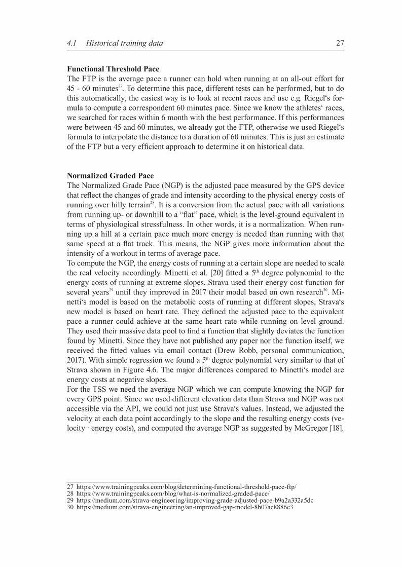
Normalized Graded PaceThe Normalized Grade Pace (NGP) is the adjusted pace measured by the GPS device that reflect the changes of grade and intensity according to the physical energy costs of running over hilly terrain28. It is a conversion from the actual pace with all variations from running up- or downhill to a “flat” pace, which is the level-ground equivalent in terms of physiological stressfulness. In other words, it is a normalization. When run-ning up a hill at a certain pace much more energy is needed than running with that same speed at a flat track. This means, the NGP gives more information about the intensity of a workout in terms of average pace. To compute the NGP, the energy costs of running at a certain slope are needed to scale the real velocity accordingly. Minetti et al. [20] fitted a 5th degree polynomial to the energy costs of running at extreme slopes. Strava used their energy cost function for several years29 until they improved in 2017 their model based on own research30. Mi-netti‘s model is based on the metabolic costs of running at different slopes, Strava‘s new model is based on heart rate. They defined the adjusted pace to the equivalent pace a runner could achieve at the same heart rate while running on level ground. They used their massive data pool to find a function that slightly deviates the function found by Minetti. Since they have not published any paper nor the function itself, we received the fitted values via email contact (Drew Robb, personal communication, 2017). With simple regression we found a 5th degree polynomial very similar to that of Strava shown in Figure 4.6. The major differences compared to Minetti‘s model are energy costs at negative slopes.For the TSS we need the average NGP which we can compute knowing the NGP for every GPS point. Since we used different elevation data than Strava and NGP was not accessible via the API, we could not just use Strava‘s values. Instead, we adjusted the velocity at each data point accordingly to the slope and the resulting energy costs (ve-locity ∙ energy costs), and computed the average NGP as suggested by McGregor [18].

27 https://www.trainingpeaks.com/blog/determining-functional-threshold-pace-ftp/28 https://www.trainingpeaks.com/blog/what-is-normalized-graded-pace/29 https://medium.com/strava-engineering/improving-grade-adjusted-pace-b9a2a332a5dc30 https://medium.com/strava-engineering/an-improved-gap-model-8b07ae8886c3

4.1 Historical training data

28

Figure 4.6: Grade Adjusted Pace model by Strava30

4.1 Historical training data

29

4.2 Neural network as a regression modelIn the following, we describe the underlying neural network (NN) of our model in terms of structure and hyperparameters. We assume that basic terminology and tech-niques of NNs are known and do not have to be explained in detail.

4.2.1 Neural network

A NN consists of nodes (neurons) organized into layers which can be stacked upon each other. Starting with an input layer where the initial data comes in, the values flow through hidden layers, consisting of an arbitrary number of nodes, until an output layer summarizes all computations of the nodes and outputs a prediction. Each node has a weight and an activation function to change when active the data coming through by multiplication. A network needs to be trained to give correct predictions, in other words, the weights need to be adjusted in an optimization process. During training the predicted output gets compared to the real value and the error gets fed back via back-propagation to adjust the weights. When reaching the smallest error, the network is trained and is able to predict for any new input a correspondent output. The more nodes per layer are added and the more layers get stacked upon each other, the more complex and powerful the network gets. Additionally, the optimization process gets more dif-ficult and time consuming. Since we have only limited training data, we decided for a network with an input layer, one hidden layer with 5 nodes and one output layer with a single node (see Figure 4.7).

4.2 Neural network as a regression model

Figure 4.7: Architecture of neural network

30

In general, NNs are able to perform different tasks like classification, clustering, re-gression etc. depending on the inner structure and output layer. While classification typically uses a form of logistic regression in the final layer of the network to output values between 1 and 0, regression maps continuous input to continuous output. The task we want to perform is a regression task with multiple independent variables. Sev-eral features need to be mapped to the estimated race time. A NN is a powerful and complex mathematical structure with lots of options and hy-perparameters. Some might say a NN is overqualified to do a simple regression task and cumbersome to use. However, NNs are a huge topic in research and have not been investigated extensively for race time prediction. We compared results of the mod-els performances with different other methods provided by scikit-learn31 like Elastic Net regression, Support Vector Machines or Nearest Neighbors, but could not achieve similar results.

4.2.2 Technical implementation

To implement the NN we used Tensorflow32 which is an open source software library originally developed by Google. Tensorflow is graph based which means all math-ematical operations get represented as nodes in a graph while the data flows as tensors through the graph. The library is available in Python and provides a high-level API in form of classes that represent parts of a NN. This makes it easy to use, even for begin-ners. If more complexity and control is needed a low-level API can be used. What characterizes a NN is the inner structure of the layers, the so-called model. To build the regressor for our prediction task, we used Tensorflow‘s Estimator classes which gave us the opportunity to implement the model with just a few lines of code. Like mentioned above, the model consists of an input layer, one hidden layer and an output layer. The input layer just takes the features and passes each through a separate node to the hidden layer. The hidden layer consists of 5 nodes with an Exponential Lin-ear Unit (ELU) as activation function. The standard activation function for regression is a Rectified Linear Unit (ReLU) but can suffer from turning inactive, therefore we chose an ELU which additionally gave slightly better results [5]. As machine learning algorithms can suffer from overfitting, we added regulariza-tion to our NN. Regularization improves the model’s generalization by putting not too much weight on non-relevant features. We used L1- and L2-Regularization (Elastic Net) in the hidden layer to keep the weights quite small and to put almost no weight on insignificant features (feature selection). Additionally, we added a dropout layer, another very popular regularization method to prevent overfitting. Dropout randomly drops nodes and their weights to prevent the network to adapt too much to a feature. Co-dependencies and sensitivity to specific weights get reduced what results in a better generalization.

31 http://scikit-learn.org/stable/supervised_learning.html32 https://www.tensorflow.org/

4.2 Neural network as a regression model

31

During the training phase the prediction errors get backpropagated to the weights to adjust them. We chose the standard error metric Mean Squared Error (MSE) in minute units. Optimization on the MSE is done by the Adam optimization algorithm with a learning rate of 0.01. The Adam algorithm uses learning rates for each weight and adapts them while training. For all training tasks 40,000 training steps were used which gave overall the best results. All input data is standardized before fed into the network.As Evaluation metric we used MSE, Root Mean Squared Error (RMSE), Mean Abso-lute Error (MAE) and Accuracy. RMSE can be seen as the standard deviation of the prediction error on the test set. MAE is self-explanatory and the accuracy is a metric to value the prediction compared to the real time (1 - absolute error ÷ actual time). We elucidate more about the evaluation metric and the methods used below in the evalua-tion sections of the both approaches. In the following, the two approaches to predict race time are presented in detail with the feature selection for each model.

4.2 Neural network as a regression model

32

4.3 Race time prediction with neural networkThe complexity of the model gets determined by the number of features. All features should have some relationship to the dependent variable which the NN tries to find during training. To capture the relations in the data, enough training data is needed. Therefore the amount of available training data somehow limits the number of features and the complexity of the model. Since we try to predict races, it would make sense to use old races for training. Depending on the athlete, the average number of finished races in our training set lies between 5 and 20 races. It is almost impossible to capture the relationship of 7 features on a dependent variable with just 20 training samples. We did tests using just races in the training set and got very varying results. For some athletes it work pretty good for others not. The main problem is that the evaluation of the model is done by splitting the training data to a training and test set what results in an even smaller training set. The question arises, is it important to use only races in a training set or are we actu-ally looking for the fastest performances over all different distances? That means, for a specified group of distances we select the fastest activities plus all races, to get an overview how an athlete is capable to perform at that distances. Nevertheless, perfor-mances done in training are mostly slower than races and therefore, to differentiate training from races, we added a categorical feature isRace. To find the fastest activities, we first used the clustering algorithm k-means to group all activities in 5 clusters. The 5 clusters should cover distances around 5 k, 10 k, half marathon, marathon and one spare for either between 10 k and half marathon or between half marathon and marathon. The clustering is done in two dimensions: the distance and the elevation gain. K-means is not deterministic, therefore we can get dif-ferent clusters each time. But since we only need the clusters to get the fastest activities for different distances, that is not an issue. To get a better start seed than the standard k-means we chose k-means++ [1] to avoid a suboptimal clustering. After having the clustered activities, we selected for each cluster the fastest activities and added them to the training set. By fastest we mean activities with an average NGP higher than the mean NGP of all activities in the cluster. The clustering guarantees that activities get selected evenly over all distances and accounts for the decrease of aver-age pace for longer distances. Taking just the fastest activities without clustering would most presumably result in picking only short distances. Figure 4.8 shows the clustering of k-means on activities of one athlete and the fastest activities in terms of NGP.

4.3 Race time prediction with neural network

Figure 4.8: K-means clustering with k = 5. All red activities were selected as fastest activities within the cluster.

33

4.3.1 Activity based approach

First, we start with the approach that is based on the activity as a whole. Training and races get valued by the parameters that characterize the overall performance. Detailed analysis of the workouts elevation profile will be covered in the second approach. Most of the research done in related work is based on the activity as a whole, thus our first approach as well.

Analysis and feature selectionTo train our model, a set of features need to be selected that represent the activity and the state and capabilities of an athlete the best. Race time is the dependent variable we want to predict and the label of the training data. Distance is the first and clearly most significant feature. Since our topic of the thesis includes races with significant elevation changes, elevation gain is an important feature that highly affects the aver-age pace, which is basically a function of distance and time. As mentioned before, the energy costs of running uphill are much higher than running on level ground or down-hill [20]. In analyzing all available activities, we stated that velocity decreases almost linearly beyond 200 m of elevation gain (see Figure 4.9). As mentioned above, elevation gain alone does not tell much about the profile, there-fore the climb score and the percentage of the hilliness need to be added to the feature set. We set the hilliness in relation to the climb score to check if we get additional in-formation and found, that the climb score is very widely spread beyond a hilliness of 60 %. Additionally, the hilliness has no linear relationship to the elevation gain. The performance in a race is correlated to the fitness and the pre-fatigue of an athlete, basically a summary of the last training weeks. To model these factors, we imple-mented the TSB model like described above. For feature selection, we just need to calculate the “fitness” (CTL) and “fatigue” (ATL) before each activity. Both values provides information about the physical state of the athlete before the activity and what performance time could be achieved. It is not a very precise summary of the training, but summarizes very individually the workload done in the last weeks.

4.3 Race time prediction with neural network

Figure 4.9: Relationship between elevation gain and velocity of all available activities. Red line is the best fitted line.

34

The average VO2max of the last 6 weeks, as another summary in terms of work done speed-wise, concludes the list of features. The VO2max of an workout like we com-puted it, is dependant on the distance, the needed time and the elevation changes. In consequence, we cannot use it in relation to the activity to predict. Instead, we used an average VO2max of all activities done in the last 6 weeks. This follows the assump-tion that an athlete achieves a fast performance if the precompetitive training included some fast workouts. Analysis of our activity set shows that the Normalized Graded Pace (NGP) increases with increasing values of average VO2max (see Figure 4.10). The same could be found for races only.

List of all features for the activity based approach to predict race time:

• activity distance

• elevation gain, hilliness, climb score

• Acute Training Load, Chronic Training Load

• average VO2max (6 weeks)

• isRace

Label: activity time

4.3.2 Segment based approach

The second approach uses parts of the first approach but goes one step further by ana-lyzing the elevation profile of the activity. Since the topic of the thesis includes predic-tions on routes with significant elevation changes, we tried to break down the activity in segments to predict on them. The activity as a whole can be seen as a large segment without paying respect to the underlying elevation profile. What we did, is splitting the “large” segment into smaller segments based on the slope of the elevation profile. As a consequence, we predicted on a small part of the activity but with a constant gradient.

4.3 Race time prediction with neural network

Figure 4.10: Relationship between the average VO2max of last 6 weeks and NGP. Red line is the best fitted line.

35

Summing up the single predictions, we get a prediction on the activity as a whole. This approach developed from the original topic idea of predicting the perfect pacing plan, what incorporates splitting the activity into segments and predicting optimal times for them. This method predicts a sort of pacing plan without knowing the target time. It learns how an athlete performed on a certain gradient within a certain activity. To not separate the segments from each other, we set them in context to the activity they belong to.

Analysis and feature selectionThe first step before feature selection is the splitting of the activity into segments. In the first part of the implementation chapter we described, how we obtained and smoothed the elevation data to get a more realistic elevation profile. The finding of the segments is actual a very easy straightforward algorithm, that processes the elevation data and generates a segment as long as the gradient is within a certain range. We de-fined six different gradient classes from flat over medium slope to very steep, positive and negative. The slope of a data point is determined over the two neighbor points. Every segment has a minimum length to prevent noise. Knowing the length, the gradient and the position within the activity is enough to represent a detailed elevation profile and are the most important features of a segment. The start of the segment within the activity helps to keep the segment in context with the activity. A segment towards the end of the activity might be slower than the pre-ceding segments due to fatigue, while the last segment might be faster due to kicking at the end. Additionally, we added a feature for the elevation gain done so far. Knowing how much elevation has to be transcended, might influence the pace of preceding segments. Information about the activity itself are the distance and the overall elevation gain.To enlarge the training data we used the same method used in the first approach. K-means clustered the activities into 5 groups from which we selected the fastest activi-ties. The selected activities were split into their segments which formed the data set for training.

List of all features for the segment based approach to predict race time:

• activity distance, activity elevation gain

• segment start distance, segment length, segment gradient, elevation gain done

• isRace

Label: segment time

4.3 Race time prediction with neural network

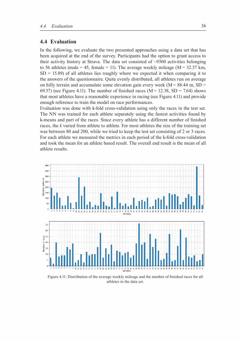
36

4.4 EvaluationIn the following, we evaluate the two presented approaches using a data set that has been acquired at the end of the survey. Participants had the option to grant access to their activity history at Strava. The data set consisted of ~9300 activities belonging to 56 athletes (male = 45, female = 11). The average weekly mileage (M = 32.37 km, SD = 15.89) of all athletes lies roughly where we expected it when comparing it to the answers of the questionnaire. Quite evenly distributed, all athletes run on average on hilly terrain and accumulate some elevation gain every week (M = 88.44 m, SD = 69.37) (see Figure 4.11). The number of finished races (M = 12.38, SD = 7.64) shows that most athletes have a reasonable experience in racing (see Figure 4.11) and provide enough reference to train the model on race performances. Evaluation was done with k-fold cross-validation using only the races in the test set. The NN was trained for each athlete separately using the fastest activities found by k-means and part of the races. Since every athlete has a different number of finished races, the k varied from athlete to athlete. For most athletes the size of the training set was between 80 and 200, while we tried to keep the test set consisting of 2 or 3 races. For each athlete we measured the metrics in each period of the k-fold cross-validation and took the mean for an athlete based result. The overall end result is the mean of all athlete results.

4.4 Evaluation

Figure 4.11: Distribution of the average weekly mileage and the number of finished races for all athletes in the data set.

37

4.4.1 Activity based approach

The model reached a mean accuracy of 91.28 % on the complete data set. RMSE lays at 6:45 min and MAE at 5:44 min. Figure 4.12 shows the distribution of the average accuracies and RMSEs of all athletes. The plot of the accuracies indicates that a few athletes (5, 6, 10, 16, 18, 37, 43, 48, 53) could achieve values of over 95 % accuracy and one even reached 98 %. What we also can state, that there are outliers (1, 12, 19, 31) with average accuracies around 80 - 85 % and RMSEs over 15 minutes (12, 31, 34, 42). Figure 4.13 depicts a histogram of the average prediction errors per athlete to illustrate the density in terms of minutes. Most of the errors lay around and slightly under 5 min-utes tapering off around 10 minutes with some outliers under 20 minutes. We reviewed the predictions that were achieved for the evaluation in each cross-vali-dation period. We found that the model performed very well on single test races with a large amount of elevation gain, peaking at accuracies of 98 - 99 %. Even races of the same athletes with almost no elevation gain reached the same accuracy dimensions in an other evaluation period. This shows that the model was able to capture the relation-ship between distance, elevation gain and time. Furthermore, we found that athletes, who do a lot of workouts with high elevation gain in training (1, 13, 19, 25, 54), could not achieve very high accuracies. It is possible that for those athletes the “fast” activities found by k-means restrain the predictions on fast races.

4.4 Evaluation

Figure 4.12: RMSEs and accuracies of activity evaluation per athlete. Red line marks the mean of 6:45 min and 91.28 % respective.

38

4.4.2 Segment based approach evaluation

Evaluation was done in the same way like described in the first approach. K-fold cross-validation was done on the basis of the activities to be able to reassemble the segments to activities and evaluate the overall time. In detail, this means that the test set con-sisted only of segments belonging to the races determined by cross-validation. The general evaluation was done on activity basis because this is what we want to predict. Besides the accuracy of the predicted race time, we introduce the similarity of the pre-dicted pacing plan which is the mean of the single segment accuracies. The similarity measures how much the predicted plan resembles the actual pacing. It is important to mention, that the similarity gives more information about the quality of the predic-tions, since it is the mean of the segment-based accuracies, while the overall activity accuracy does not account for negative and positive errors of segment predictions. If the segments of an activity have equally large positive and negative prediction errors in seconds, predictions would result in 100 % activity accuracy and a much lower similarity. Furthermore, a prediction with a low similarity and a high accuracy might be unfeasible to reach for an athlete because it exceeds all capabilities.Our model reached a mean accuracy of 83.89 % and a mean similarity of 63.15 % on the complete data set. RMSE lays at 15:22 min and MAE at 11:59 min. On segment ba-sis we achieved a mean accuracy of 53.69 % (RMSE = 108.06 sec, MAE = 69.77 sec). The model failed to predict any useful values for two athletes with negative accuracies. These large errors downgrade the overall performance significantly. Without the failed predictions the mean accuracy increased to 89.82 % and the mean similarity to 76.41 % (RMSE = 9:08 min, MAE = 7:33 min). Figure 4.14 shows per athlete the dis-tribution of the race time accuracies and the similarities of the predicted pacing plan. For most athletes the similarity is much lower than the accuracy. Positive and negative prediction errors on segment basis cancel each other out which leads to a higher ac-curacy on activity basis.

4.4 Evaluation

Figure 4.13: Histogram of average activity prediction errors per showing MAE and RMSE.

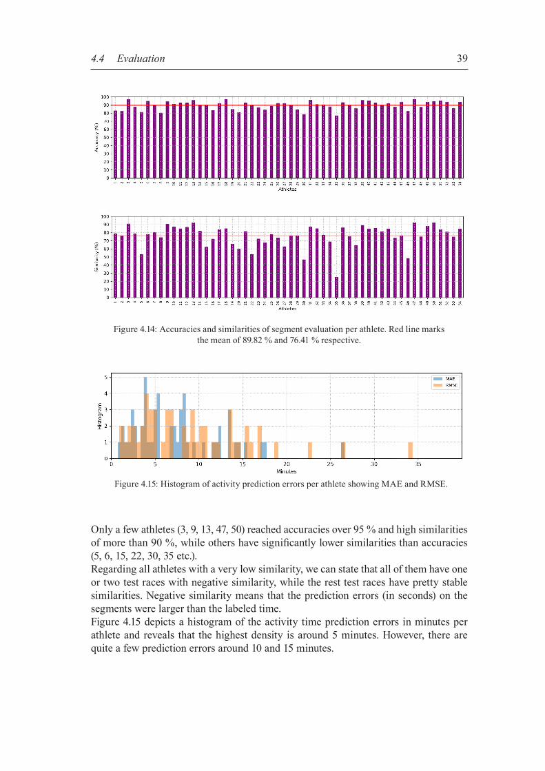
39

Only a few athletes (3, 9, 13, 47, 50) reached accuracies over 95 % and high similarities of more than 90 %, while others have significantly lower similarities than accuracies (5, 6, 15, 22, 30, 35 etc.). Regarding all athletes with a very low similarity, we can state that all of them have one or two test races with negative similarity, while the rest test races have pretty stable similarities. Negative similarity means that the prediction errors (in seconds) on the segments were larger than the labeled time. Figure 4.15 depicts a histogram of the activity time prediction errors in minutes per athlete and reveals that the highest density is around 5 minutes. However, there are quite a few prediction errors around 10 and 15 minutes.

Figure 4.15: Histogram of activity prediction errors per athlete showing MAE and RMSE.

Figure 4.14: Accuracies and similarities of segment evaluation per athlete. Red line marks the mean of 89.82 % and 76.41 % respective.

4.4 Evaluation

40

4.5 Comparison of the two approachesTo conclude this chapter, we compare in the following the presented approaches re-garding advantages and evaluation results. The activity based approach has the ad-vantage, that it does not heavily depend on the accuracy of the elevation profile. Little errors in the computation of the elevation gain or the hilliness have little impact on the prediction. Where in the segment based approach, little errors in the elevation profile are huge errors on segment basis.Additionally, the first approach uses the features ATL and CTL which represent the state of the athlete in terms of fitness and fatigue. Adding those to the feature set of the second approach, would make the model extremely complex. ATL and CTL are measurements on the level of activities, while fatigue within an activity would require a new measurement. The main advantage of the segment based approach is the fact, that the model not only predicts a summed up race time but a pacing plan or pacing strategy. What is more, the predicted pacing plan is a feasible plan since it is based on athlete specific reference.Concerning the technical evaluation of the two approaches, it can be stated that the activity based model performed very well on the provided data set reaching a mean accuracy of over 91 %, including some outliers under 85 % which decreased the over-all results slightly. We could show that predictions on single races with a reasonable amount of elevation gain could achieve accuracies of over 98 %, which gives reason for the assumption that the model captured the influence of elevation gain on race time.The second model on basis of segments could not perform as good as the first one. Re-garding alternating similarities within the athlete set and the discrepancies of accuracy and similarity, we can state that this approach is very sensitive to faulty or abnormal data. We have found that doing the evaluation several times, for some athletes the re-sults varied a lot. This can be due to optimization problems during training (weights initialization, local minima). What decreased both model‘s mean accuracy are single test races of athletes in one or two of k periods with significantly bad predictions. Why these single predictions have such large errors is not clearly visible. It is possible that the recorded activity time is not correct because the athlete forgot to push the stop button or that the athlete performed not at a maximum capacity. Even though we reviewed all activities tagged as races, there might be activities that do not represent a “good” performance and should be excluded. Additionally, some athletes did not tag activities on Strava or just tagged a part of them. Without knowing the athletes in the data set and monitoring exactly their race history, it is difficult to find a “correct” test set of races. Athletes or coaches could make an informed decision which activity should be added to the test set and which does not really represents a race performance.

4.5 Comparison of the two approaches

41

5 User study

We conducted a final study to evaluate the quality of the predictions in a real scenario and to compare our approach to standard methods like Riegel‘s formula. In this chapter we compare the results to each other and to the evaluation results from the previous chapter.

5.1 Setting and participantsThe “Bank 1 Saar Silvesterlauf Saarbrücken” was selected as race as it has significant elevation changes and enough competitors from amateurs to professionals. The course goes through the woods and has around 150 m elevation gain over 10 km distance. Since it is dated at the end of the year temperatures are quite low and people use it as a year closing race. This year almost 900 athletes finished the race within a range of 31 - 108 minutes. For our study we used two ways to recruit participants. First, before the race we posted online in a Facebook running group and on Strava. Additionally, we spread flyers on race day. Second, we directly approached finishers via Strava (i.e. commenting on their race activity). All participants received a short description of the topic of the thesis. As incentive they received a race time prediction and could win an online coupon. Participation could be done before and after the race since the subjects did not receive a prediction or any other information before the race that could influence their perfor-mance. Participation was completed with granting us access to the Strava training data and with successfully finishing the race.In total 12 athletes took part in the study (male = 9, female = 3) with race times be-tween 39 and 54 minutes (M = 43:56 min, SD = 5:24). The following values (related to all activities of the athletes, max. 2 years old) give information about the level and the specialization of the participants: weekly mileage (M = 31.56 km, SD = 14.12), average elevation gain per activity (M = 122.12 m, SD = 99.62), the number of races (M = 7.58, SD = 6.51). Figure 5.1 shows the number of finished races per subject. Two athletes only finished one race in the past, at least available for us on Strava. For the rest, almost 5 or more finished races is a reasonable number to make a good prediction. Regard-ing average elevation gain per activity, one athlete stands out with ~ 400 m. It can be assumed that the athlete does a lot of mountain running which also explains the slow average training pace of 6:06 min/km. Furthermore, 3 other athletes train on very flat terrain with less than 50 m elevation gain per workout what could be a disadvantage for a race with 150 m elevation gain.

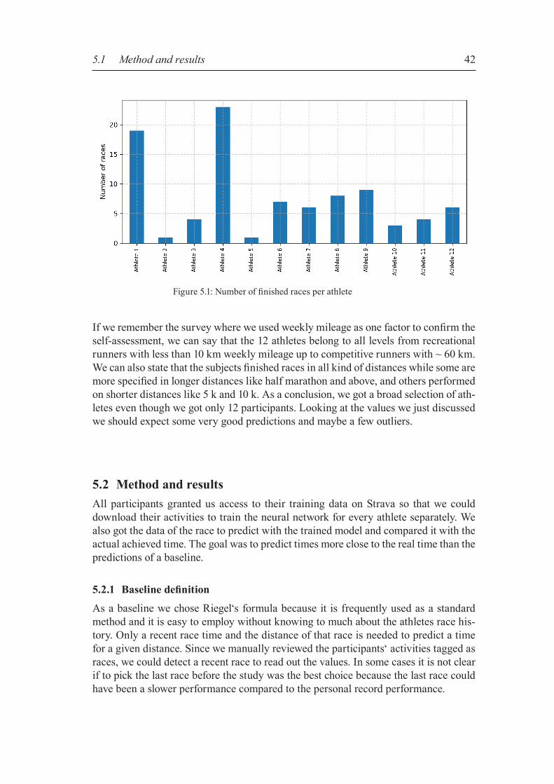
42

If we remember the survey where we used weekly mileage as one factor to confirm the self-assessment, we can say that the 12 athletes belong to all levels from recreational runners with less than 10 km weekly mileage up to competitive runners with ~ 60 km. We can also state that the subjects finished races in all kind of distances while some are more specified in longer distances like half marathon and above, and others performed on shorter distances like 5 k and 10 k. As a conclusion, we got a broad selection of ath-letes even though we got only 12 participants. Looking at the values we just discussed we should expect some very good predictions and maybe a few outliers.

5.2 Method and resultsAll participants granted us access to their training data on Strava so that we could download their activities to train the neural network for every athlete separately. We also got the data of the race to predict with the trained model and compared it with the actual achieved time. The goal was to predict times more close to the real time than the predictions of a baseline.

5.2.1 Baselinedefinition

As a baseline we chose Riegel‘s formula because it is frequently used as a standard method and it is easy to employ without knowing to much about the athletes race his-tory. Only a recent race time and the distance of that race is needed to predict a time for a given distance. Since we manually reviewed the participants‘ activities tagged as races, we could detect a recent race to read out the values. In some cases it is not clear if to pick the last race before the study was the best choice because the last race could have been a slower performance compared to the personal record performance.

5.1 Method and results

Figure 5.1: Number of finished races per athlete

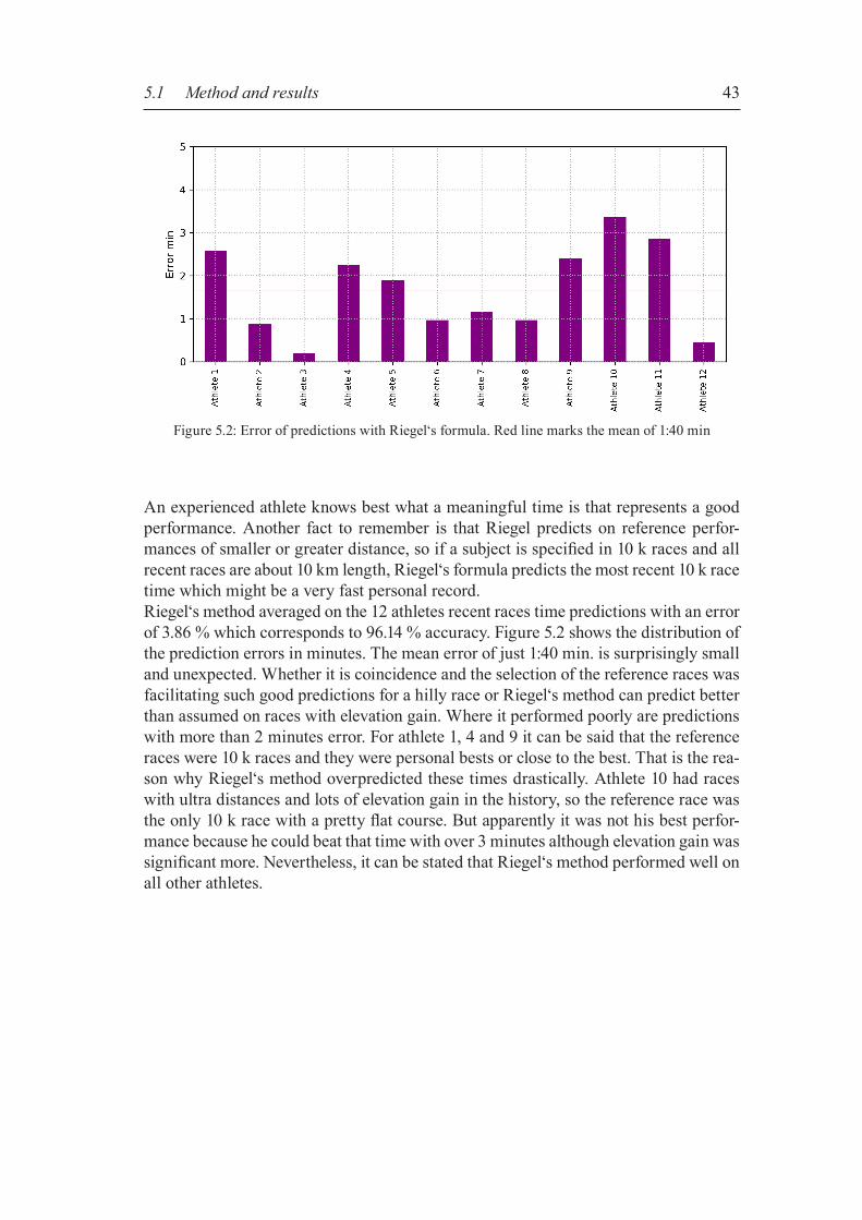
43

An experienced athlete knows best what a meaningful time is that represents a good performance. Another fact to remember is that Riegel predicts on reference perfor-mances of smaller or greater distance, so if a subject is specified in 10 k races and all recent races are about 10 km length, Riegel‘s formula predicts the most recent 10 k race time which might be a very fast personal record. Riegel‘s method averaged on the 12 athletes recent races time predictions with an error of 3.86 % which corresponds to 96.14 % accuracy. Figure 5.2 shows the distribution of the prediction errors in minutes. The mean error of just 1:40 min. is surprisingly small and unexpected. Whether it is coincidence and the selection of the reference races was facilitating such good predictions for a hilly race or Riegel‘s method can predict better than assumed on races with elevation gain. Where it performed poorly are predictions with more than 2 minutes error. For athlete 1, 4 and 9 it can be said that the reference races were 10 k races and they were personal bests or close to the best. That is the rea-son why Riegel‘s method overpredicted these times drastically. Athlete 10 had races with ultra distances and lots of elevation gain in the history, so the reference race was the only 10 k race with a pretty flat course. But apparently it was not his best perfor-mance because he could beat that time with over 3 minutes although elevation gain was significant more. Nevertheless, it can be stated that Riegel‘s method performed well on all other athletes.

Figure 5.2: Error of predictions with Riegel‘s formula. Red line marks the mean of 1:40 min

5.1 Method and results

44

5.2.2 Prediction and evaluation

Activity based predictionFor the activity based approach the model was trained for each athlete separately like described in the previous chapter and predictions were made on the left out target race. The model reached an average accuracy of 92.48 % (SD = 7.29) what corresponds to an average error of 3:16 min (SD = 3:10 min). Figure 5.3 shows the distribution of the ac-curacies and the prediction errors in minutes. Three subjects stand out with significant higher errors. Athlete 10 peaks with 10:04 min error and an accuracy of only 75.93 %. As mentioned above, athlete 10 does a lot of slow mountain running what can explain the positive offset of the prediction. The high error of athlete 5 can be explained with only one finished race and an average historical elevation gain of 20 m. The error of athlete 12 can be explained with the small ratio of races vs. activities selected by k-means (6 vs. 204) and a relative slow average training pace. 50 % of the predictions have an error smaller than 2 minutes with a max. accuracy of 99.08 % for athlete 7. Athlete 7 did a fair amount of hilly workouts (> 110 m) and finished 6 races in all standard distances including one with some elevation gain. This prerequisites could have led to the almost perfect prediction.

Figure 5.3: Accuracies and errors of activity based predictions. Red line marks the mean of 92.48 % and 3:16 min respective.

5.1 Method and results

45

Segment based predictionFor the segment based approach the model was trained on the calculated segments and used the same method for evaluation like described in the previous chapter‘s evalua-tion section. The target race consisted of 20 - 30 segments for which we predicted the times and reassembled the activity by summing those times up. The variance of the number of segments comes from the GPS data recorded by the running watches. We used for each athlete their own GPS data of the target race since all of the historical training was tracked by this device. Taking data from just one device for all athletes would have mixed the different accuracy levels of the running watches. We achieved an average accuracy of 88.2 % and an average similarity of 81.54 %. Figure 5.4 shows the distribution of the accuracies and similarities. Only 4 subjects reached a similarity over 90 %. The model failed to predict any useful outcome for ath-lete 9 with a here stated similarity of 41.5 %. This result was achieved after countless trials. Further, athlete 10 has also a very low similarity of 61.5 % but stable predictions. The reasons for the bad predictions athlete 10 are the same like in the first approach. For athlete 9 it is difficult to find an explanation for the failure because predictions in the first approach were promising. A possible explanation that the model predicted times for some segments way too fast and unfeasible to reach, could be due to the fact that athlete 9 did not much of elevation changes (~ 19 % hilliness). And the segments done with a positive gradient could have been hill sprints or similar intensive workouts.

Figure 5.4: Accuracies and similarities of segment based predictions. Red line marks the mean of 88.2 % and 81.54 % respective.

5.1 Method and results

46

Quite a few accuracies significantly improved compared to the first approach however accuracy, relating to the summed up time of all predicted segment times, depends on the equal distribution of positive and negative segment prediction errors. When com-paring the similarity with the accuracy we can see that e.g. for athlete 12, regardless of the similarity of 86.6 %, an accuracy of 97.14 % was achieved because of the equaliza-tion of positive and negative prediction errors. An extreme example is athlete 10 where accuracy is smaller than similarity due to a constant positive prediction error. Figure 5.5 shows the profile of the race and the segment based prediction errors of athlete 10.

5.3 Discussion and improvementTo compare the two approaches and the baseline we summarize the results in the fol-lowing. The activity based prediction approach reached an accuracy of 92.48 %, the segment based prediction approach a similarity of 81.54 % and the baseline an ac-curacy of 96.14 %. Clearly, we could not beat the baseline with all participants in the data set. The baseline had a quite evenly distributed error over all athletes where most notably the first approach had quite a few outliers with high error. Figure 5.6 shows the relationship between actual time and predicted time of all athletes and makes outliers better visible. It also reveals that all outliers of the first approach were underestimated performance times where the second approach did significant over- and underpredic-tions. The baseline also predicted a few times too fast in cases where the reference race was a flat fast performance. Compared to the evaluation results of the two models in chapter 4, the similarity is significantly higher (~ 5 %) while the accuracy increased only slightly (~ 1 %). To improve the overall performance of the two models we removed outliers that obvi-ously are hard to predict and weakened the power of the model. If we consider the sub-set of all participants who had finished at least 4 races and did 20 km per week mini-mum on average, we are left with 7 athletes satisfying this constraints. Two training sessions at 10 km distance would result in 20 km weekly mileage and is a reasonable

5.3 Discussion and improvement

Figure 5.5: Elevation profile with prediction error of athlete 10. All errors are positive and add up to a worse accuracy than similarity.

47

amount to count as serious training effort. Four races can give a good overview of stan-dard race distances. The evaluation of this subset improved the average accuracy of the activity based approach to 95.25 % and the similarity of the segment based approach to 87.82 %. Even a better selection of the participants could not beat the baseline but we could improve the accuracy almost 3 % and the similarity more than 6 % respectively. The low number of participants also could have impaired the overall result.

Figure 5.6: Relationship between actual time and predicted time

5.3 Discussion and improvement

48

6 Conclusion

In the following chapter we summarize the essential aspects of the work done in this thesis. We evaluate the achievements of the overall goal and how much we could im-prove compared to related work. At the end we present possible future work and exten-sions to this thesis.

6.1 SummaryMotivated by an online questionnaire on the quality of current race time calculators and what factors influence athlete‘s performance, we presented two approaches for race time prediction on historical training data of athletes. We quantified the perfor-mance of our two prediction models in an evaluation and a user study.

We started off by examining related work in the area of race time/performance predic-tion in running and compared standard methods and formulas to newer approaches that look more at the individual athlete and his training history. We found that re-nowned websites use Riegel‘s formula or an improved version of it, which performs very well on flat races for exemplary athletes while prediction tools including elevation gain are rare. To motivate our work by feedback from the running community, we conducted an online questionnaire where we asked the participants about their opinion of current prediction tools in the field of running, questions about pacing strategies and what pa-rameters have an impact on their running performance. Half of all participants found the quality of current predictors non-satisfying and showed a strong interest on a pre-diction application that also could suggest a pacing plan for a given race, besides stan-dard race time prediction. Most participants argued, that current predictors take only a few parameters into account to predict a race time that depends on much more values. The questionnaire gave us an overview of what runners think, that influences their performance on race day the most. With the feedback from the questionnaire in mind, we presented in the implementation chapter two approaches to predict race time on athlete specific historical training data including elevation changes. The first approach looks at the activities as a whole while the second one breaks down each activity into segments to give a better representation of the underlying elevation profile. In the section about the first approach we described how we accessed athletes‘ training data from Strava and replaced Strava‘s elevation values. With assumably better eleva-tion data from Google, we computed the first features like elevation gain, hilliness and climb score. We introduced the Training Stress Balance (TSB) model as a representa-tion of the human performance parameters: fitness and fatigue. As a last feature, we added the average VO2max of the last 6 weeks. We explained how we trained the neural network with the training set obtained by k-means and how we evaluated the model using k-fold cross-validation. We could achieve an evaluation result of 91.28 % accuracy and an RMSE of 6:45 min for the first model. We showed that the neural network can capture the impact of elevation gain on the

49

average pace and we made the assumption that with very accurately recorded test data we could even achieve better predictions.For the second approach we explained why splitting the activity into segments gives us a better representation of the elevation changes. We showed how we computed the seg-ments from the pre-smoothed elevation data. Length, gradient and start of the segment within the activity are the segment features complemented by activity related features. Evaluation of the segment approach was also done with k-fold cross-validation and achieved an accuracy of 89.82 % and a similarity of 76.41 % (RMSE = 9:08 min). The results were significantly lower than those of the first approach. The model even failed to make useful predictions for two athletes. We stated that the segment based predic-tions are very sensitive and in same cases unstable over multiple evaluation periods. At the end of the implementation phase we conducted a user study to evaluate the quality of the predictions in a real scenario and to test wether our approach can beat a standard method like Riegel‘s formula. The study was organized at a local race over 10 km with ~ 150 m elevation gain. 12 athletes participated in the study whose race time predictions reached an average accuracy of 92.48 % with an error of 3:16 min. using the first prediction approach. The segment based approach achieved a slightly lower accuracy of 88.2 % and a similarity of 81.54 %. After removing some outliers with insufficient racing history and very little weekly mileage, we improved the activ-ity based predictions to an accuracy of 95.25 % and the segment based predictions to a similarity of 87.82 %. In the study, both approaches could not beat Riegel‘s formula which gained a very high accuracy of 96.14 %. The final study showed that our models performed much better on real data. Therefore, we can conclude that the models are good at generalizing to new data.

6.2 Evaluation of the overall goalFirst of all, we managed to include elevation gain into race time predictions and achieved high accuracies. Our first model captured very well the impact of elevation on an athlete‘s average pace knowing only three elevation related features. The second model performed slightly worse on segment based features with a sensitivity to faulty or abnormal training data. But a huge contribution of the segment based approach is the fact that it does not only predict a single race time but also a pacing plan. In the final study, our goal was to predict better times than a baseline, what we shortly missed. Even after removing some outliers the first model could not reach Riegel‘s ac-curacy. If the model really performed worse than the baseline or if the selection of the reference races for Riegel‘s formula was just poor, is not clear. To find out if our models could reach same error rates than those presented in the re-lated work chapter or even performed better, we compare the evaluation results in the following. Ruiz-Mayo et al. [23] included elevation gain and quite a few other training related features in the regression task and reached a mean absolute error of ~ 7 min-utes. Our first model is with 5:44 min significantly better, although we cannot compare the accuracy of the predictions. Millett et al. [19] who explored locally weighted linear

6.2 Evaluation of the overall goal

50

regression and a Hidden Markov Model to predict race times on historical race data convinced with a 3.8 % error rate using the HMM (3.9 % for regression). However, locally weighted linear regression failed to give any useful prediction for 10 % of all races. The HMM outperformed our first model by almost 5 % error. Definitely, both data sets can not be compared and it seems that they used data of “competitive” ath-letes all having more than 10 races finished so far. Blythe et al. [3] reached an average prediction error on elite marathon performances of 3.6 min (3:36 min) which is not exactly comparable to an evaluation all on different distances. Fact is, that our model’s MAE of 5:44 min for predictions on recreational athletes over all kind of distances is pretty good in contrast to 3:36 min on elite mara-thon performances.To compare our second model, we use Smyth and Cunningham’s work [24,25] where they presented a very specific approach how a recommender system can be used in a marathon to reach a new personal best. They achieved errors of 4 - 5 % on average and race plan similarities of more than 90 %. Their method outperformed our segment based approach drastically. An advantage of our method is that we do not necessarily require a finished marathon on the same or a similar course to predict a marathon race time. Additionally, our approaches take the historical training data of the athlete for the predictions into account, while their predictions are only possible with the appropriate training. Looking at the comparison of the models, we can conclude that we definitely reached our goal and that our approaches have a huge potential for improvement in future work, presented in the following.

6.3 Future workNext, we present some ideas and future improvements that would continue the work started with this thesis. As we saw, the basis of the work done in this thesis relies on the accuracy of the GPS coordinates and elevation data. Little errors in the GPS data can lead to bigger errors in elevation data. Research could be done if there exist algorithms that could efficiently perform GPS coordinate correction or some kind of matching to existing tracks and path segments. The only problem with matching algorithms is that runners typically never follow straight lines, they cross streets or leave pathways. Regarding the eleva-tion data accuracy, most certainly Google provides currently the best quality available for free with a large coverage. Own analysis on the relationship between elevation changes and heart rate or velocity could lead to better more accurate elevation profiles. If heart rate values with a high precision were available they could together with veloc-ity give information about the underlying elevation profile. Better elevation data could possibly improve predictions by the second approach, which highly depends on the elevation profile. Another improvement of the models could be reached by adding more features to the model. At the current state all activities and races have no subjective rating by the ath-

6.3 Future work

51

lete. All performances get the same weight no matter if an athlete performed only at 70 % of his capacity or all-out. A rating of performances would differentiate races at same distances but with different race times. Sometimes runners use races as faster training runs or unexpected problems occur during a race. With an additional feature the model could learn how much effort an athlete put into the achieved performance. Doing this automatically is very difficult because a lot of uncertain assumptions would have to be done. New activities could employ a rating done manually by the athlete. Further features that could be added are weather or altitude. Typically hot conditions and high altitude have the same effects on the performance of athletes but adding those factors would make the model more powerful. The question would be, how much heat or altitude affects the endurance of the individual athlete. It would need a reasonable amount of training data recorded in such conditions. Or an other option would be to penalize the predicted time in a more general way to account for exertion caused be heat or altitude. Furthermore, parameters that have an effect on the overall race time, like those men-tioned by the participants of our survey, could be added. For example sleeping quality or motivation could easily be implemented and slightly tweak the predicted time. To pick up the original idea of an optimal pacing strategy, the second prediction ap-proach is very close to that idea. It predicts a pacing plan for segments based on the elevation profile. It predicts how fast an athlete can run certain segments. We did some experiments with adding the target time as a feature to turn the race time prediction into suggesting a pacing strategy. Results were pretty promising, we could achieve even a higher accuracy and similarity. The model knows what the available time is and tries to distribute it to the segments according to the other features. The pacing plan adapted very well when changing to a slower or faster activity time, what means it also can be used for slower and possibly faster races. The idea of an optimal pacing strategy would require a similar approach like Smyth et al. [24,25] suggest in their work. Any kind of pacing plan could be displayed on modern GPS running watches to help runners dur-ing a race to not overpace and save enough energy for upcoming hills. An even further step, that could be implemented once running watches have more computational power and memory, is the possibility to update a plan in real time according to circumstances during a race. This would mean that a runner falling behind a suggested plan could get an updated version of the original plan that may compensate the lost time. A last idea to improve the performance of the neural networks, would be to use training techniques like “Transfer Learning” to overcome the problem of the small training set. It would also help to learn facts that the athlete have not experienced so far. In the first step, the neural network would learn general facts of running on a large data set and initialize the weights accordingly. An athlete specific fine tuning would individualize the model in a second step. One could compare this procedure to first using Riegel‘s formula as a general basis and then adjusting the variables to the individual athlete.

6.3 Future work

52

53

Bibliography

[1] Arthur, David; Vassilvitskii, Sergei. K-Means++: The Advantages of Careful Seeding. In Proceedings of the eighteenth annual ACM-SIAM symposium on Discrete algorithms, 2007, pp. 1027-1035.

[2] Berndsen, Jakim; Lawlor, Aonghus; Smyth, Barry. Running with Recommen-dation. In Proceedings of Second International Workshop on HealthRecommender Systems co-located with ACM RecSys 2017, (RecSys’17).

[3] Blythe, Duncan A. J.; Király, Franz J. Prediction and Quantification of Indivi-dual Athletic Performance of Runners. PLoS ONE, 2016, 11(6).

[4] Candès, Emmanuel J.; Recht, Benjamin. Exact matrix completion via convex optimization. Foundations of Computational mathematics, December 2009, Vol. 9, p. 717.

[5] Clevert, Djork-Arné; Unterthiner, Thomas; Hochreiter, Sepp. Fast and Ac-curate Deep Network Learning by Exponential Linear Units (ELUs). Under Review of ICLR2016, November 2015.

[6] Daniels, Jack; Gilbert, Jimmy. Oxygen Power: Performance Tables for Distan-ce Runners. Tempe, Ariz., 1979.

[7] Douglas, David H.; Peucker, Thomas K. Algorithms for the Reduction of the Number of Points Required to Represent a Digitized Line or Its Caricature. Cartographical: The International Journal for Geographic Information and Geovisualization, October 1973, Vol. 10, pp. 112-122.

[8] Elliott, James B. Marathon pacing and elevation change. Cornell University Library, October 2012.

[9] Faulkner, J.; Arnold, T.; Eston, R. Effect of accurate and inaccurate dis-tance feedback on performance markers and pacing strategies during running. Scand J Med Sci Sports, August 2010, pp. 176-183.

[10] Gardner, James B.; Purdy, J. Gerry. Computer generated track scoring tables. Medicine and science in sports, 1970, Vol. 2 No. 3, pp. 152 - 161.

[11] Gosztyla, Amy E.; Edwards, David G.; J. Quinn, Timothy; Kenefick, Robert W. The impact of different pacing strategies on five-kilometer running time trial performance. Journal of Strength and Conditioning Research, 2006, pp. 882–886.

54

[12] Hausswirth, Christophe; Le Meur, Yann; Bieuzen, Francois; Brisswalter, Jeanick; Bernard, Thierry. Pacing strategy during the initial phase of the run in triathlon: influence on overall performance. Eur J Appl Physiol, April 2010, pp. 1115–1123.

[13] Higdon, H. Marathon – The Ultimate Training Guide, Rodale Books, 4th edi-tion (2011).

[14] Jin, Tiffany. Predicting Pace Based on Previous Training Runs, Stanford: Ma-chine Learning (2014), http://cs229.stanford.edu/proj2014/ [Online; last acces-sed 02/02/2018].

[15] Kolodner, Janet L. An introduction to case-based reasoning. Artificial Intelli-gence Review, March 1992, Vol. 6 No. 1, pp. 3–34.

[16] Li, Yang; Hu, Peng; Fan, Qingsong; Guo, Fenglin. The Generalization Based on 3 Dimensional Douglas-Peucker Algorithm in New DEM Model. Education Technology and Training & Geoscience and Remote Sensing, December 2008, pp. 283-286.

[17] Lima-Silva, Adriano E.; Bertuzzi, Romulo C. M.; Pires, Flavio O.; Barros, Ronaldo V.; Gagliardi, João F.; Hammond, John; Kiss, Maria A.; Bishop, David J. Effect of performance level on pacing strategy during a 10-km running race. Eur J Appl Physiol, March 2010, pp. 1045-1053.

[18] McGregor, Stephen; Fitzgerald, Matt. The Runner‘s Edge. Ebook, https://books.google.de/books?id=dcWybPNh6GwC&printsec=frontcover&dq=run-ners+edge&hl=de&sa=X&ved=0ahUKEwjhi_fznY_ZAhWEb1AKHdvWCb-0Q6AEIKjAA#v=onepage&q=runners%20edge&f=false [Online; last acces-sed 02/02/2018], p. 42.

[19] Millett, Matt; Melanson, TJ. Predicting Running Times from Race History. Stanford: Machine Learning (2015), http://cs229.stanford.edu/proj2015/247_re-port.pdf [Online; last accessed 02/02/2018].

[20] Minetti, Alberto E.; Moia, Christian; Roi, Giulio S.; Susta, Davide; Ferretti, Guido. Energy cost of walking and running at extreme uphill and downhill slopes. J Appl Physiol, 2002, Vol. 93 No. 3, pp. 1039-1046.

[21] Purdy, J. Gerry. Least squares model for the running curve. Research Quarter-ly, October 1974, pp. 224-238.

[22] Riegel, Peter S. Athletic records and human endurance. American Scientist, Vol. 69, No. 3 (May-June 1981), pp. 285-290.

55

[23] Ruiz-Mayo, Daniel; Pulido, Estrella; Martínez-Muñoz, Gonzalo. Mara-thon Performance Prediction of Amateur Runners based on Training Session Data. Machine Learning and Data Mining for Sports Analytics (2016), ECML/PKDD 2016.

[24] Smyth, Barry; Cunningham, Pádraig. A Novel Recommender System for Helping Marathoners to Achieve a New Personal-Best. In Proceedings of the Eleventh ACM Conference on Recommender Systems (2017), RecSys ‘17, pp. 116-120.

[25] Smyth, Barry; Cunningham, Pádraig. Running with Cases: A CBR Approach to Running Your Best Marathon. In Proceedings of the 25th InternationalConference on Case-Based Reasoning CCBR (2017), David W. Aha and Jean Lieber (Eds.). Springer International Publishing, pp. 360–374.

[26] Tanda, Giovanni. Prediction of marathon performance time on the basis of training indices. Journal of Human Sport and Exercise, September 2011, Vol. 6 No. 3, pp. 521-520.

[27] Townshend, Andrew D.; Worringham, Charles J.; Stewart, Ian. Spontaneous pacing during overground hill running. Medicine and Science in Sports and Exercise, January 2010, Vol. 42 No. 1, pp. 160-169.

[28] Vickers, Andrew J.; Vertosick, Emily A. An empirical study of race times inrecreational endurance runners. BMC Sports Science, Medicine and Rehabili-tation, 2016, 8:26.