Embed Size (px)
Citation preview

Clemson UniversityTigerPrints
All Dissertations Dissertations
5-2008
JUDICIAL CHECKS ON CORRUPTIONAdriana CordisClemson University, [email protected]
Follow this and additional works at: https://tigerprints.clemson.edu/all_dissertations
Part of the Economics Commons
This Dissertation is brought to you for free and open access by the Dissertations at TigerPrints. It has been accepted for inclusion in All Dissertations byan authorized administrator of TigerPrints. For more information, please contact [email protected].
Recommended CitationCordis, Adriana, "JUDICIAL CHECKS ON CORRUPTION" (2008). All Dissertations. 192.https://tigerprints.clemson.edu/all_dissertations/192

JUDICIAL CHECKS ON CORRUPTION
A Dissertation Presented to
the Graduate School of Clemson University
In Partial Fulfillment of the Requirements for the Degree
Doctor of Philosophy Applied Economics
by Adriana Simona Cordis
May 2008
Accepted by: Dr. Robert D. Tollison, Committee Chair
Dr. Michael T. Maloney, Co-Chair Dr. William R. Dougan
Dr. Todd D. Kendall Dr. Cotton M. Lindsay

ii
ABSTRACT
Judicial oversight is widely regarded as an important check and balance on the
abuse of governmental power. The literature identifies two important components of this
oversight function: judicial independence and constitutional review. However, recent
work using country-level data indicates that the effectiveness of constitutional review is
largely determined by the rigidity of the constitution. My dissertation builds on this work
by investigating whether judicial independence and constitutional review are deterrents to
a specific type of abuse of power by government officials: corruption in office. Since the
appropriate way to measure corruption, which is defined as the abuse of public office for
private gain, remains an unsettled issue, I use both measures of corruption derived from
criminal convictions data and measures of corruption derived from survey data. In the
case of the former, I propose a new empirical strategy that explicitly recognizes the
distinction between the unobserved number of corrupt officials and the observed number
of convictions for corruption.
I begin by examining whether differences in judicial independence and
constitutional rigidity at the state level in the United States explain the observed variation
in the number of corruption convictions across states. I investigate these issues
empirically using annual data for the years 1996-2005. Judicial independence is assessed
by looking at judicial remuneration, method of selection, and term length. To assess
constitutional rigidity, I use the legislative majority needed in each state to propose
constitutional amendments, the provision (or lack thereof) for constitutional conventions,
and the provision (or lack thereof) for popular initiatives to amend the constitution.

iii
I find that both judicial independence and constitutional rigidity are significant
predictors of corruption. The coefficient estimates indicate that in states where judges
have a higher degree of independence (higher remuneration, merit plan selection, or
longer terms), there is less corruption. Moreover, states that have more rigid
constitutions (higher legislative majorities required to propose constitutional
amendments) experience less corruption. These findings, which are new to the literature,
suggest that policy reforms which promote judicial independence and make it more
difficult to alter constitutions have the potential to mitigate the harmful effects of
corruption that have been documented in other studies.
To develop additional insights, I conduct a similar empirical investigation in a
cross-country setting. Since I do not have data on corruption convictions at the country
level, I use several survey-based measures, from Transparency International, the World
Bank (Kaufmann et al., 2007), and the Political Risk Survey Group. My measures of
judicial independence and constitutional review are drawn from a variety of sources. I
obtain indices of judicial independence from the Economic Freedom of the World
Report, published by the Fraser Institute, from the Political Constraint Index Dataset, and
from the La Porta et al. (2004) study cited earlier. The constitutional review index is
taken from La Porta et al. (2004) as well. Like most of the literature, I analyze these
data using linear regression methods: ordinary least squares, weighted least squares, and
panel data techniques. Since data availability varies across indices, I conduct my analysis
on cross-sections of between 37 to 165 countries for various years between 1995 and

iv
2005. I then extend my analysis to panels of data with cross-sectional and time-series
observations for 1998 to 2005.
The evidence on judicial independence from the cross-country analysis is
generally consistent with that from the United States data. I find strong support in favor
of my hypothesis that higher judicial independence is associated with lower corruption
levels, ceteris paribus. This finding is robust to the way corruption and judicial
independence levels are measured, to the estimation technique, and, in general, to the
inclusion of various control variables. However, I do not find the expected relation
between corruption and constitutional rigidity. It appears that countries with more rigid
constitutions experience more corruption using the same controls as for the judicial
independence models. In their study, La Porta et al. (2004) show that constitutional
review is a guarantee of political freedom measured by indices of democracy, human
rights and political rights, but not of economic freedom. This suggests that it may be
possible to reconcile the findings from the cross-country analysis with the evidence for
the United States by gaining a better understanding of the relation between political
freedom and economic freedom.

v
DEDICATION
To Chris
vi
ACKNOWLEDGMENTS
I thank my advisors, Dr. Michael Maloney and Dr. Robert Tollison, for their
guidance, advice, and support. I am particularly grateful to Dr. Maloney for his enormous
help throughout my graduate studies. His enthusiasm and belief in my abilities gave me
the confidence necessary to reach this point in my career. I am also grateful to Dr.
William Dougan, Dr. Matt Lindsay, Dr. Todd Kendall, and Dr. John Warner who
contributed greatly to my success by sharing their thoughts, ideas, and providing
comments on my research.
I thank the Earhart Foundation and the John E. Walker Department of Economics
for their generous financial support during my final year in graduate school.
Finally, I want to acknowledge the support of my family. I thank Doru and
Cristina for believing in me and helping me reach my goals. I would not have made it
without them. I thank my parents for encouraging me to pursue my dreams. I owe them
everything and I wish I could show them just how much I love them. I thank Chris,
whose love and unconditional support are my greatest source of inspiration. Te iubesc.

vii
TABLE OF CONTENTS
Page
TITLE PAGE .................................................................................................................... i ABSTRACT ..................................................................................................................... ii DEDICATION ................................................................................................................. v ACKNOWLEDGMENTS .............................................................................................. vi LIST OF TABLES .......................................................................................................... ix LIST OF FIGURES ........................................................................................................ xi CHAPTER 1. INTRODUCTION ......................................................................................... 1 2. RELATED LITERATURE ............................................................................ 6 3. JUDICIAL CHECKS AND BALANCES ON CORRUPTION .................. 10 4. EVIDENCE FROM THE UNITED STATES ............................................. 14 Empirical Strategy ................................................................................. 14 Models.................................................................................................... 17 Data ........................................................................................................ 28 Estimation Results ................................................................................. 35 Robustness ............................................................................................. 42 Conclusions ............................................................................................ 46 5. EVIDENCE FROM ACROSS COUNTRIES ............................................. 48 Empirical Specifications ........................................................................ 48 Data ........................................................................................................ 52 Results .................................................................................................... 64 Additional Robustness Checks .............................................................. 79 Conclusions ............................................................................................ 84 6. CONCLUSIONS.......................................................................................... 87
viii
Table of Contents (Continued)
Page
REFERENCES .............................................................................................................. 87

ix
LIST OF TABLES
Table Page 1. States with Most and Least Corruption Convictions per State Government Employee ................................................................. 29 2. States with Most and Least Corruption Convictions per State Resident......................................................................................... 29 3. Descriptive Statistics ................................................................................... 30 4. Detailed Description of the Corruption Convictions Variable .................................................................................................. 33 5. Test of Overdispersion ................................................................................. 34 6. Observed and Predicted Number of Corruption Convictions ...................... 36 7. Effect of Judicial Independence on Corruption in the United States .......................................................................................... 40 8. Effect of Constitutional Review on Corruption in the United States .......................................................................................... 41 9. Effect of Judicial Independence on Corruption: Robustness Checks................................................................................. 44 10. Effect of Constitutional Review on Corruption: Robustness Checks................................................................................. 45 11. Correlation Coefficients between Corruption Indicators ............................. 53 12. Countries with Highest and Lowest Corruption Scores According to the Corruption TI Index ................................................... 54 13. Countries with Highest and Lowest Corruption Scores According to the Corruption World Bank Index ................................... 55 14. Countries with Highest and Lowest Corruption Scores According to the Corruption PRS Index ................................................ 56

x
List of Tables (Continued) Table Page 15. Correlation Coefficients between Judicial Independence Indicators............................................................................................... 56 16. Countries with Most and Least Independent Judiciaries According to the Judicial Independence (I) Index ................................. 58 17. Descriptive Statistics of Cross-Country Data .............................................. 62 18a. Effect of Judicial Independence (I) on Corruption TI ................................. 68 18b. Effect of Judicial Independence (II) on Corruption TI ................................ 69 18c. Effect of Judicial Independence (III) on Corruption TI............................... 71 18d. Effect of Constitutional Review on Corruption TI ...................................... 72 19a. Effect of Judicial Independence (I) on Corruption World Bank ............................................................................................ 74 19b. Effect of Judicial Independence (II) on Corruption World Bank ............................................................................................ 75 20a. Effect of Judicial Independence (I) on Corruption PRS .............................. 76 20b. Effect of Judicial Independence (II) on Corruption PRS............................. 77 21. Effect of Judicial Independence on Corruption TI: Pooled OLS, WLS, and Panel Estimations ............................................ 81 22. Effect of Judicial Independence on Corruption World Bank: Pooled OLS, WLS, and Panel Estimations.................................. 82 23. Effect of Judicial Independence on Corruption PRS: Pooled OLS and Panel Estimations ....................................................... 83

xi
LIST OF FIGURES
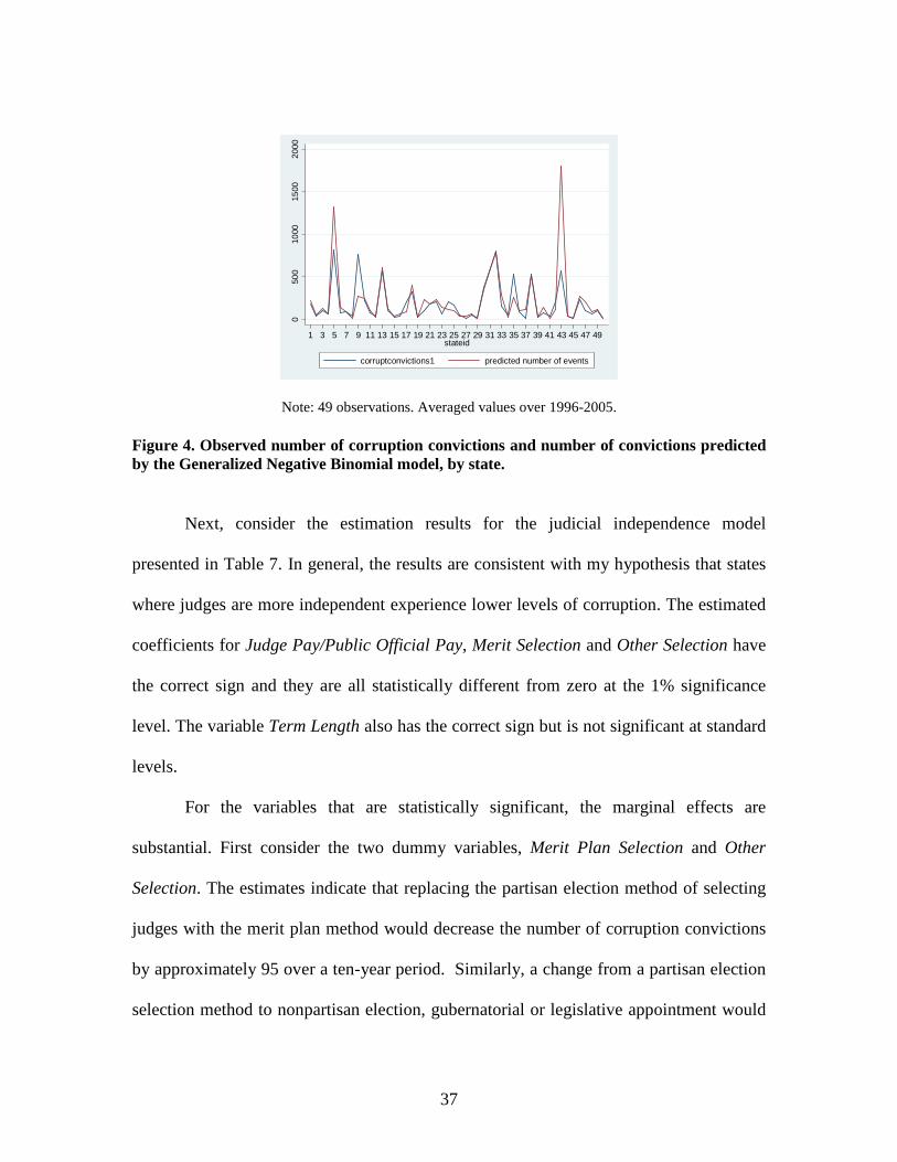
Figure Page 1. Distribution of corruption convictions (490 observations from 1996-2005)....................................................... 32 2. Distribution of corruption convictions (49 observations. Averaged values over 1996-2005) ........................... 32 3. Observed number of corruption convictions against a Poisson distribution with the same mean and a Negative Binomial distribution with the same mean and variance ....................................... 34 4. Observed number of corruption convictions and number of convictions predicted by the Generalized Negative Binomial model, by state ....................................................................... 37

CHAPTER ONE
INTRODUCTION
Over the past two centuries, judicial oversight has evolved into a cornerstone of
the system of checks and balances that is central to the United States model of
governance at both the state and national levels. The literature identifies two main ways
in which the judiciary provides checks on the power of the legislative and executive
branches: judicial independence and constitutional review. Judicial independence matters
because judges subject to the influence of the legislative or executive branches will be
less likely to decide cases in an impartial manner. Constitutional review matters because,
in addition to trying to influence judges, the legislative or executive branches may seek to
pass laws or implement policies that are designed to benefit themselves and/or their
associates. By reviewing whether such actions are constitutional, the judiciary places
limits on such self-serving behavior.
Since the actions of a state government are subject to review not only against the
provisions of the state’s constitution but also against those of the federal constitution, one
might hypothesize that there should be little difference in the effectiveness of
constitutional review from one state to another. However, if the legislature of one state
can as easily alter the state constitution as it enacts new laws, then it has much wider
latitude than the legislature of another state that has a rigid constitution. Based on this
argument, differences in constitutional rigidity across states could result in differences in
the effectiveness of the judicial review process. The frequency with which state
constitutions are altered suggests that it is necessary to consider the rigidity issue. State

2
legislatures proposed 974 constitutional amendments over my sample period, of which
78% were adopted. There were also 156 constitutional changes proposed via popular
initiatives, of which 44% were successful.
La Porta et al. (2004) provide direct evidence on the need to consider
constitutional rigidity when investigating the effectiveness of constitutional review. They
use cross-country data to investigate whether judicial independence and constitutional
review act as important guarantees of freedom. Using data for 71 countries, they find
that both of these variables are associated with greater freedom. However, the impact of
constitutional review is closely tied to the rigidity of the constitution. I build on this
work by investigating whether judicial independence and constitutional rigidity are
deterrents to a specific type of abuse of power by government officials: corruption in
office.
First, I examine the relation between corruption and both judicial independence
and constitutional rigidity in the United States using state-level data on corruption
convictions for the years 1996-2005. Judicial independence is assessed by looking at
judicial remuneration, method of selection, and term length. To assess constitutional
rigidity, I use the legislative majority needed to propose constitutional amendments, the
provision (or lack thereof) for constitutional conventions, and the provision (or lack
thereof) for popular initiatives to amend the constitution. Unlike previous studies that
use convictions data, which simply ignore the disparity between convictions and the
underlying level of corruption, I propose an empirical strategy that explicitly recognizes

3
the difference between the unobserved number of corrupt officials and the observed
number of convictions for corruption.
Since the number of officials convicted for corruption represents an unknown
fraction of the total number of corrupt officials, I assume that each corrupt official faces
some risk, i.e., probability, of being revealed as corrupt, and that this risk does not vary
across individuals within a state. This allows me to express the number of officials
convicted of corruption in each state as the outcome of ni independent Bernoulli trials
where ni is the unobserved number of corrupt officials in state i. To obtain my empirical
specifications, I model ni as a Poisson process whose mean depends on a vector of
explanatory variables, and show that this leads to a negative binomial specification for
the number of corruption convictions.
Using this specification, I show that both judicial independence and constitutional
rigidity are significant predictors of corruption. The coefficient estimates suggest that in
states where judges have a higher degree of independence (higher remuneration, merit
plan selection, or longer terms), there is less corruption. Moreover, states that have more
rigid constitutions (larger legislative majorities required to propose constitutional
amendments) experience less corruption. These findings, which are new to the literature,
suggest that policy reforms which promote judicial independence and make it more
difficult to alter constitutions have the potential to mitigate the harmful effects of
corruption documented in other studies.
To see whether my findings generalize to other settings, I also investigate the
determinants of corruption at the country level. Since I do not have data on corruption

4
convictions at the country level, I use several survey-based measures. The first is
constructed and published by Transparency International. It is a composite index,
computed as the average of surveys from up to 14 sources originating from 12
independent institutions. These surveys are based on the views of business people, risk
analysts, journalists, and the general public. The second is a new index put together by
researchers at the World Bank (Kaufmann et al., 2007). It aggregates views on corruption
form a wide range of individual surveys to obtain a “consensus” corruption index for the
years 1999-2006. The third is constructed and sold by the Political Risk Survey Group.
This index represents an assessment, by international experts, of bureaucratic and
political corruption.
My measures of judicial independence and constitutional review are drawn from a
variety of sources. I obtain indices of judicial independence from the Economic Freedom
of the World Report, published by the Fraser Institute, from the Political Constraint Index
Dataset, and from the La Porta et al. (2004) study cited earlier. The constitutional review
index is taken from La Porta et al. (2004) as well. Like most of the literature, I analyze
these data using linear regression methods: ordinary least squares, weighted least squares,
and panel data techniques. Since data availability varies across indices, I conduct my
analysis on cross-sections of between 37 to 165 countries for various years between1995
and 2005. I then extend my analysis to panels of data with cross-sectional and time-series
observations for 1998 to 2005.
The evidence on judicial independence from the cross-country analysis is
generally consistent with that from the United States data. I find strong support in favor

5
of my hypothesis that higher judicial independence is associated with lower corruption
levels, ceteris paribus. This finding is robust to the way corruption and judicial
independence levels are measured, to the estimation technique, and in general to the
inclusion of various control variables. However, I do not find the expected relation
between corruption and constitutional rigidity. It appears that countries with more rigid
constitutions experience more corruption using the same controls as for the judicial
independence models. In their study, La Porta et al. (2004) show that constitutional
review is a guarantee of political freedom measured by indices of democracy, human
rights and political rights, but not of economic freedom. This suggests that it may be
possible to reconcile the findings from the cross-country analysis with the evidence for
the United States by gaining a better understanding of the relation between political
freedom and economic freedom.
The rest of the dissertation is organized as follows. Chapter 2 reviews the
relevant literature on both judicial oversight and corruption-related issues. Chapter 3
presents the theoretical framework and develops the hypotheses to be tested. Chapter 4
presents the empirical evidence from the United States. I first discuss the empirical
strategy and the models. Then I describe the data and present the empirical results.
Chapter 5 presents the cross-nations empirical evidence. Chapter 6 provides a few
concluding remarks.
6
CHAPTER TWO
RELATED LITERATURE
Over the past three decades, beginning with Susan Rose-Ackerman (1975),
economists have shown a growing interest in analyzing the causes and consequences of
corruption. Much of the recent research on corruption is conducted in cross-country
settings [see, e.g., Shleifer and Vishny (1993), Mauro (1995), Ades and di Tella (1997),
Ades and di Tella (1999), La Porta et al. (1999), Treisman (2000), Adserà et al. (2000),
Kunicova and Rose-Ackerman (2002), Braun and Di Tella (2004), Gokcekus and
Knörich (2005)].
This literature documented that weak governments are an incubator for high
corruption levels, and that corruption retards economic growth, and lowers investment
and private savings (Mauro, 1995). In addition, the amount of corruption in a country is
positively correlated with the variance of inflation (Braun and di Tella, 2004) and
negatively correlated with Protestant religion traditions, histories of common law, long
exposure to democracy (Treisman, 2000), or the level of openness, measured as ratio of
total trade (exports and imports) to gross domestic product (Gokcekus and Knörich,
2005). The presence of democratic mechanisms of control and of an informed electorate,
measured through the frequency of newspaper readership, are negatively correlated to
corruption (Adserà et al., 2000), and presidential systems, in particular nationwide
closed-list proportional representation in conjunction with presidentialism, i.e., where
party leaders rank candidates and voters only select political parties, are positively
associated with corruption (Kunicova and Rose-Ackerman, 2002).
7
Besides the empirical findings from the cross-national settings, there is a growing
literature on corruption in the United States that exploits the availability of both criminal
justice and survey data. Studies such as Meier and Holbrook (1992), Welch and Hibbing
(1997), Goel and Nelson (1998), Alt and Lassen (2003), Glaeser and Saks (2004), and
Maxwell and Winters (2005) show that many of the findings from the international
literature regarding the economic, historical, cultural and political determinants of
corruption appear to hold within the United States as well.
Corruption is negatively correlated with education and per capita income, and
positively correlated with ethnic heterogeneity and income inequality (Glaeser and Saks,
2004). Government size, measured as state government expenditures, has a strong
positive correlation with corruption (Goel and Nelson, 1998), and institutional variables
related to the openness of the political system, such as direct initiatives, campaign
expenditure restrictions, or open primaries, are negatively correlated with corruption (Alt
and Lassen, 2003). In addition, historical/cultural factors, such as urbanism, Irish/ Italian
ancestry, and crime rates, are positively related to corruption, and among the political
forces, voter turnout lowers corruption, while party competition is weakly negatively
associated with corruption (Meier and Holbrook, 1992).
Studies that investigate the relation between corruption and characteristics of the
judicial system are scarcer. Legal origins have been shown to matter in cross-country
studies [La Porta (1999), La Porta (2004), and Treisman (2000)]. In particular, the
evidence suggests that the legal system is more effective, and hence corruption is lower,
in countries with common law systems as opposed to civil law systems. La Porta et al.

8
(2004) investigate whether judicial checks and balances act as a guarantee of freedom.
Using data for 71 countries around the world, they provide evidence that judicial
independence and constitutional review are associated with (i) greater economic freedom,
measured by the security of property rights, the lightness of government regulation, and
the infrequency of state ownership, and (ii) greater political freedom, measured by
indices of democracy, political rights, and human rights.
One of the few studies to directly address the impact of checks and balances on
corruption using United States data is Alt and Lassen (2005). They argue that various
forms of checks and balances are precautionary devices against government corruption.
To test this hypothesis, they use Boylan and Long’s (2003) survey of State House
reporters’ perceptions of public corruption as the dependent variable, along with data on
the presence of divided government and on judicial selection. Their findings show that
states in which the executive and the legislative branches of government are controlled by
different political parties and states in which judges are elected rather than appointed
experience lower corruption levels. This latter result contradicts the long-standing belief
that appointed judges are more independent [Hall (1987), Hall (2001), Feld and Voigt
(2003), Besley and Payne (2003), Hanssen (2004), Sobel and Hall (2007)]. Alt and
Lassen (2005) also show that the effect of a judiciary accountable to the public is stronger
under a unified government.
Other studies, such as Wallis (2004) and Glaeser and Goldin (2004), provide a
historical overview of the corruption issue for the years 1842 to 1852 and 1815 to 1975,
respectively, and illustrate how the institution of checks and balances evolved to ensure

9
an effective control between different levels of government. Glaeser and Goldin (2004)
argue that corruption decreased significantly between the mid 1870s and 1920, and
attribute this result to the increased costs that corrupt politicians faced as the news media
began reporting corruption everywhere in America and “the full apparatus of modern
checks on corruption were in place.”

10
CHAPTER THREE
JUDICIAL CHECKS AND BALANCES ON CORRUPTION
Corruption is defined as the abuse of public office for private gain (World Bank).
Susan Rose Ackerman (1999, p. 9) notes that corruption is a “symptom that something
has gone wrong in the management of the state” and that “institutions designed to govern
the interrelationships between the citizen and the state are used instead for personal
enrichment and the provision of benefits to the corrupt.” This definition allows
classifying as corruption a plethora of acts ranging from “low-level” corruption, such as
payments to obtain licenses or benefits, payments to avoid delay in obtaining a public
service, and payments for relief from government regulation, taxes, or custom duties, to
“high-level” corruption, such as payments to win major procurement contracts or
concessions from the government, payments to retain monopoly power, or payments to
pass laws or to get a favorable interpretation of the laws.
The starting point for my analysis of the impact of judicial checks on corruption is
the assumption that once they acquire a position of trust, public office holders may abuse
power, i.e., take actions that are not congruent with the interests of voters.1 Persson et al.
(1997) identify two mechanisms designed to align the interests of public officials and
voters: the electoral process and separation of powers. The electoral process is a way of
disciplining public officials by denying them the right to make decisions in the future,
while separation of powers serves to control and limit the power of public officials while
1 This assumption can be motivated by appealing to the theory of political agency as formulated by Barro (1973), Ferejohn (1986), Persson et al. (1997), and Maskin and Tirole (2004). The theory focuses on the divergence of interests between voters (principals) and their political representatives (the agents).

11
in office. According to Persson et al. (1997), separation of powers, and particularly the
institution of checks and balances, limits abuse of power by creating conflicts of interest
between the legislative and the executive, or by requiring agreement of both branches in
the law-making process. A central result of Persson et al. (1997) is that, under appropriate
checks and balances, separation of powers improves the accountability of public
officials.2
For the separation of power model of governance to function properly, it must
ensure the division of power between all three branches of government: the executive, the
legislative and the judiciary. Montesquieu (1748, p.155) writes “it has eternally been
observed that any man who has power is led to abuse it; he continues until he finds
limits…So that one cannot abuse power, power must check power.” This thinking
influenced the writers of the United States Constitution, who acknowledged that “there
can be no liberty where the legislative and the executive powers are united in the same
person or body of magistrates, or if the power of judging be not separated from the
legislative and executive powers” (Madison 1788, p.263). Within this governance model,
the Anglo-American institution of checks and balances attributes a special role to the
judiciary.
2 Landes and Posner (1975) put forth a different argument that has similar implications. They develop a theory of the independent judiciary in an interest group perspective. Under their model, interest groups make wealth transfers to legislators in return for favorable legislation. Since the wealth transfers are larger when legislation lasts beyond the term of the enacting legislature, politicians have incentives to find methods of increasing the permanency of laws. Establishing an independent judiciary, which makes it more costly for future regimes to change existing policies, is one such method.

12
According to Hayek (1960), there are two ways in which the judiciary provides
checks and balances: judicial independence and constitutional review. First consider
judicial independence. Hayek (1960, p.210) writes “Rules must not be made with
particular cases in mind, nor must particular cases be decided in the light of anything but
the general rule…This requires independent judges who are not concerned with any
temporary ends of government.” La Porta et al. (2004) point out that judicial
independence is especially important in cases where the government is itself a litigant or
in lawsuits where one of the litigants is politically connected and the executive wants the
court to favor its ally.
Independent judges are free of political pressure exercised by the executive, the
legislative or the public and thus free to implement an impartial judgment without fear of
retribution. Susan Rose-Ackerman (1999, p. 151) notes that:
A politically dependent judiciary can facilitate high-level corruption, undermine reforms, and override legal norms. When the judiciary is part of the corrupt system, the wealthy and the corrupt operate with impunity, confident that a well-placed payoff will deal with any legal problems. […]Business deals may be structured inefficiently to avoid encounters with the judicial system, and ordinary people may be systematically taken advantage of because they lack access to an impartial system of dispute resolution. Bidding wars may develop in which parties on opposing sides compete in making payoffs.
The above arguments, and the fact that the states mirror the separation of power model at
the federal level, allow me to form my first testable hypothesis. States or nations that
confer judges relatively greater judicial independence experience lower corruption.
Next consider constitutional review. Constitutional review is designed to
reinforce citizens’ guarantees against the law-making power of the legislature. As La
Porta et al. (2004, p.447) note, both “the executive and the legislature may enact policies
13
and pass laws that benefit themselves, democratic majorities, or allied interest groups.”
By means of constitutional review, these policies can be declared unconstitutional by the
court if they are in conflict with the legal code or with the constitution itself.3 However,
constitutional review becomes a less effective check as the constitution becomes less
rigid. If the legislature of a state can as easily alter the state constitution as it writes new
laws, then it has much wider latitude than the legislature of a state that has a rigid
constitution. Furthermore, in a government where the judiciary exercises a reliable check
on the other branches, policies cannot be implemented unless all separate bodies agree,
which makes use of corrupt practices to pass a law very costly. I thus derive my second
testable hypothesis. States or nations where constitutions are more rigid, i.e., it is more
costly to propose amendments from a legislative perspective, should experience lower
corruption.
3 The foundation for exercising judicial review in the United States is considered to be Marbury v. Madison 5 U.S. 137 (1803), a decision pronounced by Chief Justice John Marshall.

14
CHAPTER FOUR
EVIDENCE FROM THE UNITED STATES
In order to test my hypotheses, I have to make a decision about how to measure
corruption. This is an unsettled issue in the literature. Typically, researchers use either
survey-based measures or measures derived from data on criminal convictions. Both
types of measures have their drawbacks. Survey-based measures are clearly subjective.
Thus, one can always question their accuracy. There is no way to know whether the
participants in the survey are biased, or whether they are sufficiently knowledgeable to
express an informed opinion.
Convictions-based measures, on the other hand, are clearly a noisy proxy for the
true number of corrupt officials. Not every corrupt official is exposed, tried, and
convicted for his or her corrupt acts. Previous studies that use convictions-based
measures simply ignore this fact. In this paper, I develop an empirical specification that
explicitly recognizes the difference between the unobserved number of corrupt officials
and the observed number of convictions. My approach is presented below.
4.1. Empirical Strategy
Let ni be the number of corrupt government officials in state i. The value of ni is
inherently unobservable. Suppose, however, that some of these officials are revealed to
be corrupt through the judicial process (i.e., indicted and convicted for corrupt acts). To
model this process, I assume that every corrupt official faces some risk of being revealed
as corrupt. Specifically, I assume that each official is revealed to be corrupt with some
15
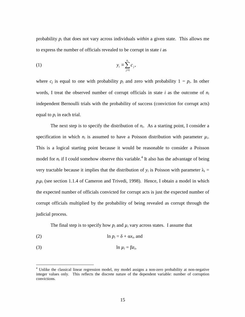
probability pi that does not vary across individuals within a given state. This allows me
to express the number of officials revealed to be corrupt in state i as
(1) ∑=
=in
jji cy
1
,
where cj is equal to one with probability pi and zero with probability 1 − pi. In other
words, I treat the observed number of corrupt officials in state i as the outcome of ni
independent Bernoulli trials with the probability of success (conviction for corrupt acts)
equal to pi in each trial.
The next step is to specify the distribution of ni. As a starting point, I consider a
specification in which ni is assumed to have a Poisson distribution with parameter µi.
This is a logical starting point because it would be reasonable to consider a Poisson
model for ni if I could somehow observe this variable.4 It also has the advantage of being
very tractable because it implies that the distribution of yi is Poisson with parameter λi =
piµi (see section 1.1.4 of Cameron and Trivedi, 1998). Hence, I obtain a model in which
the expected number of officials convicted for corrupt acts is just the expected number of
corrupt officials multiplied by the probability of being revealed as corrupt through the
judicial process.
The final step is to specify how pi and µi vary across states. I assume that
(2) ln pi = δ + αxi, and
(3) ln µi = βzi,
4 Unlike the classical linear regression model, my model assigns a non-zero probability at non-negative integer values only. This reflects the discrete nature of the dependent variable: number of corruption convictions.
16
where xi is a vector of covariates that I believe should capture variation in law
enforcement effectiveness across states (per capita expenditures on police, per capita
number of prosecutors, etc.) and zi is a vector of covariates that I believe should capture
variation in the level of corruption across states (judicial independence, constitutional
review, racial fractionalization, etc.).5 The final specification is:
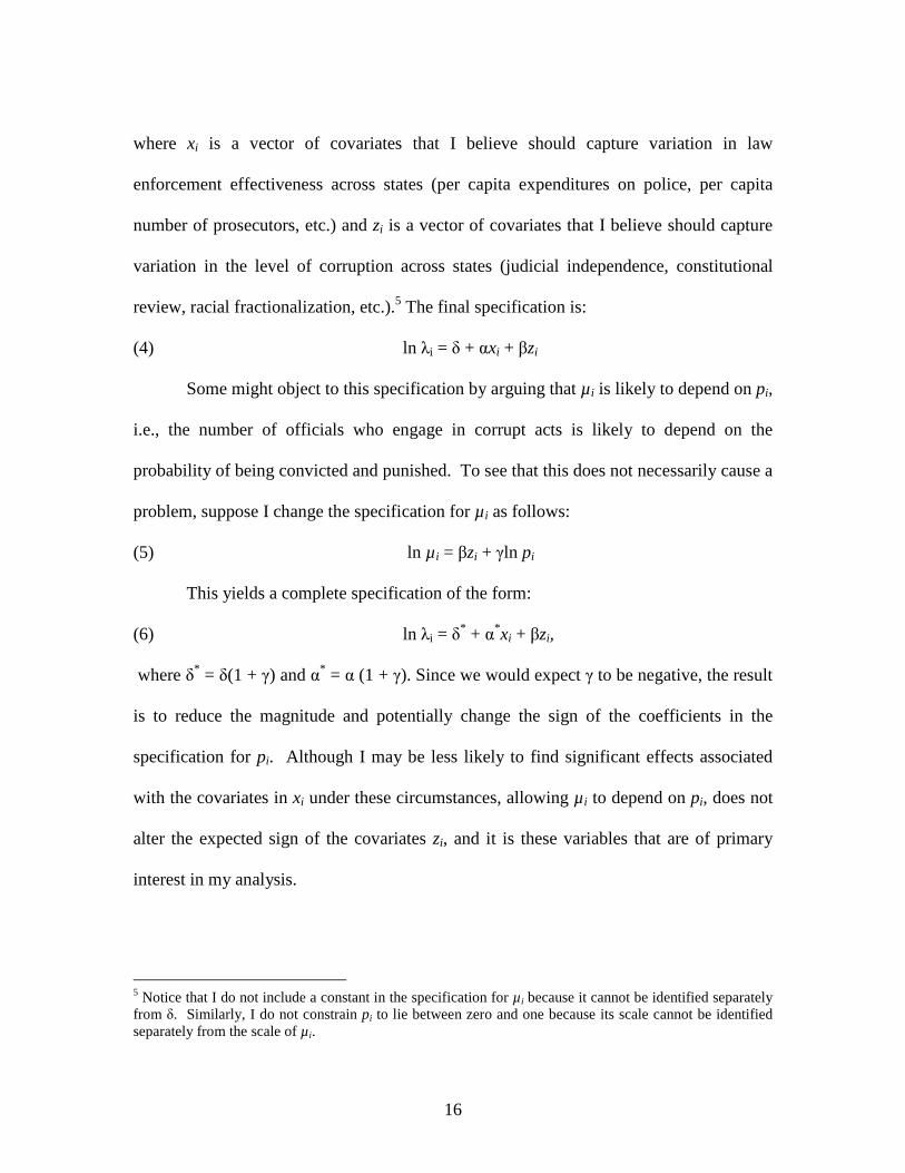
(4) ln λi = δ + αxi + βzi
Some might object to this specification by arguing that µi is likely to depend on pi,
i.e., the number of officials who engage in corrupt acts is likely to depend on the
probability of being convicted and punished. To see that this does not necessarily cause a
problem, suppose I change the specification for µi as follows:
(5) ln µi = βzi + γln pi
This yields a complete specification of the form:
(6) ln λi = δ* + α*xi + βzi,
where δ* = δ(1 + γ) and α* = α (1 + γ). Since we would expect γ to be negative, the result
is to reduce the magnitude and potentially change the sign of the coefficients in the
specification for pi. Although I may be less likely to find significant effects associated
with the covariates in xi under these circumstances, allowing µi to depend on pi, does not
alter the expected sign of the covariates zi, and it is these variables that are of primary
interest in my analysis.
5 Notice that I do not include a constant in the specification for µi because it cannot be identified separately from δ. Similarly, I do not constrain pi to lie between zero and one because its scale cannot be identified separately from the scale of µi.

17
This Poisson model is useful for illustrating my general approach to the
estimation problem. However, it neglects unobserved heterogeneity, which may be
problematic. I will therefore use a more general specification for the empirical analysis
in the paper. Instead of assuming that ni has a Poisson distribution with parameter µi, I
assume that it has a Poisson distribution with parameter µivi where vi is a random
unobserved heterogeneity term due to specification error such as unobserved omitted
exogenous variables. With vi given, the previous discussion implies that the conditional
distribution of yi is Poisson with parameter λi = piµivi. To complete the specification, I
assume that vi has a gamma distribution and integrate out to obtain the marginal
distribution of yi (see section 4.2.2 of Cameron and Trivedi, 1998). It is negative
binomial with mean mi = piµi.
4.2. Models
La Porta et al. (2004) look at the impact of judicial independence and
constitutional review on economic and political freedom across countries by estimating
two linear regression models. The first model examines the effect of judicial
independence measures, and the second examines the effect of constitutional review
measures. I use a similar strategy to analyze the corruption data. First, I estimate a
negative binomial regression model that examines the effect of judicial independence on
corruption convictions. Next, I estimate a negative binomial regression model that
examines the effect of constitutional review on corruption convictions. I conduct the

18
analysis using data for 49 states for the years 1996-2005.6 In each case, the dependent
variable is the number of public officials (local, state, and federal) convicted in federal
court of a corruption-related crime, i.e., a crime involving abuse of public trust by
government officials.
4.2.1. Judicial Independence
To estimate a negative binomial model, I need to specify how the number of
corruption convictions in state i is related to the judicial independence measures, the law
enforcement effectiveness measures, and the covariates used as control variables. This is
accomplished by specifying the mean of the negative binomial distribution, mi. I use the
following specification for the mean:
(7) ln mi = ln(Full Time Government Employees)i+β0 + β1ln(Judge Pay/Public
Official Pay)i + β2(Merit Plan Selection)i + β3(Other Selection)i + β4(Term
Length)i + β5ln(FBI Agents)i + β6ln(Police protection)i + β7(Racial
Fractionalization)i
Note that I use the number of Full Time Government Employees as the exposure
variable for the model.7 My choice of variables to measure judicial independence reflects
a number of considerations. Article 3 of the United States Constitution provides for an
independent judicial branch.8 However, significant variation exists across states
6 I exclude the state of New Mexico from my analysis because data on the number of corruption convictions was not available for all of the years 1996 to 2005. 7 That is, the logarithm of Full Time Government Employees is used as an explanatory variable but its coefficient is constrained to equal one. This has the same effect as dividing the number of corruption convictions by the number of full time government employees. 8 Article 3 states that “Judges, both of the supreme and inferior courts shall hold their offices during good Behavior, and shall at stated Times, receive for their Services, a Compensation, which shall not be

19
pertaining to the three major constituents of judicial independence: remuneration of
judges, method of selection, and term length.9 I exploit this variation in my empirical
analysis. Four variables, Judge Pay/Public Official Pay, Merit Plan Selection, Other
Selection and Term Length are used to account for the independence of the state
judiciary. Judge Pay and Term Length pertain to the chief justice of the court of last
resort in each state, while Merit Plan Selection and Other Selection relate to the selection
of all judges of the Supreme Court.
The remuneration variable, Judge Pay/Public Official Pay, is expected to be
negatively correlated with the number of corruption convictions per capita. Common
observation tells us that judges’ monetary rewards often do not approach the salaries they
could earn in other jobs, such as practicing as private lawyers or even teaching as
university professors. Susan Rose-Ackerman (1999) notes that the independence of
judges is seriously threatened when they are underpaid and work under conditions much
worse than lawyers and their assistants. Inadequate pay decreases the expected cost of
accepting bribes. Judges’ pay, relative to that of the average public official, provides an
indication of the importance attached to the integrity of the judiciary.
There are five distinct procedures used to select judges across the United States:
partisan election, nonpartisan election, legislative appointment, governor appointment,
and an appointment-election hybrid named merit plan selection. There are six states in
which judges run as members of a political party, 15 states in which the elections are diminished during their Continuance in Office.” However, the United States Constitution does not speak to the organization and structure of the judiciary at the state level. 9 Feld and Voigt (2003) use these three variables along with others, such as case allocation rules, stability of institutional arrangements within which courts operate or requirement of publishing the decisions of courts, in order to construct an index of de jure judicial independence across 71 countries around the world.

20
nonpartisan, i.e., judges do not reveal their political affiliation,10 and seven states in
which judges are selected by appointment of the governor or of the legislature. This
leaves 21 other states in which judges are selected by merit plan. These methods of
judicial selection did not change very much across states over the 1996-2005 period.11
I will briefly explain some of the main aspects of these selection methods below.
Hanssen (2004) presents a history of the origins and evolution of judicial selection
methods after the American Revolution. He argues that the first state constitutions made
judges highly accountable to legislatures, the heroes of the Revolution, which were
regarded as “more reliable representatives of the people.” This was soon to be changed as
it became apparent that a government dominated by the legislature needs an effective
third party to monitor and limit legislative abuses. State constitutions were rewritten
providing for judicial elections (circa 1850) intending to protect the courts from the
legislature and thus to make them more independent. Judicial partisan elections also
proved to be disappointing since they were subject to manipulation, and thus there was a
movement towards nonpartisan election (circa 1910) and the merit plan (1913). Hanssen
(2004, p.431) concludes that “Each new procedure was developed in order to increase the
independence of state judges and was then superseded by a newer procedure, owing in
large part to unanticipated agency problems.”
10 A Supreme Court decision, Republican Party of Minnesota v. White 536 U.S. 765(2002) ruled that the requirement of judges not to discuss political issues is unconstitutional, and thus gave judges the right to tell voters about their positions on specific political and legal issues that might come before them. 11 In 2000, Arkansas adopted Amendment 80 which changed the judicial selection method from partisan to nonpartisan elections. Furthermore, in 2002, North Carolina passed the Judicial Campaign Reform Act which established nonpartisan elections for Supreme Court judges effective 2004. However, these changes do not affect the significance of the results.

21
Partisan elections embody an inherently political process by requiring judges to
run for office in the same way as politicians. This may force judges to solicit campaign
contributions from special interest groups, political parties and even lawyers or possible
litigants. This results in dependent judges who may feel obliged to be responsive to the
wishes of those who contributed to their election.
Merit selection12 was proposed both as a means of separating judges from politics
and as a way to call attention to professional criteria for selecting judges, such as
qualifications, experience, education, training and age. Under this procedure, a
nominating commission comprised of both lawyers and non-lawyers present the governor
with a list of nominees from which to select an appointee. When the stated term expires,
usually after a year, the judge stands for reelection with no party affiliation and no
opponent. The judge who is retained serves the prescribed term of office. It seems
reasonable to believe that judges selected through this process will have more time to
spend on the matters that are brought before them than judges who stand for election.
There is a general consensus in the existing literature that judges selected through
partisan elections are the least independent, while judges selected through the merit plan
procedure are the most independent, i.e., insulated from political pressure. A number of
previous studies provide evidence pointing to the inferiority of selection through partisan
elections.13 Thus, Hall (1987), in a Louisiana case study, shows that electoral incentives
12 Merit selection was endorsed by the ABA in 1937. It is also called the “Missouri plan,” Missouri being the first state to adopt it in 1940. 13 Criticism of judicial election dates back to 1835, when Alexis de Tocqueville (1954, p. 289) wrote: “Some other state constitutions make the members of the judiciary elective, and they are even subjected to frequent reelections. We venture to predict that these innovations will sooner or later be attended with fatal
22
discourage judges from dissenting on highly controversial issues. Hall (2001) finds that,
when deciding on death penalty cases, elected judges who have views contrary to those
of the voters and the court majority, tend to vote with the majority rather than dissent, to
strategically minimize electoral opposition. Tabarrok and Helland (1999) find evidence
that partisan judicial elections are associated with larger trial awards on average,
especially so in decisions against out of state businesses, supporting their argument that
partisan elected judges have an incentive to redistribute wealth from out-of-state
defendants (nonvoters) to in-state plaintiffs (voters). Hanssen (2002), using a sample of
37 state courts, argues that merit plan procedures render judges more independent of
political pressure, which leads to more disputes that litigate rather than settle.
Specifically, he finds that merit plan selection is associated with 18% to 32% more filings
in state supreme courts between 1985 and 1994. Besley and Payne (2003) show that there
are fewer employment discrimination filings per capita in states in which judges are
appointed, and Sobel and Hall (2007) show that the partisan nature of elections is the
primary reason for lower judicial quality in states that use elections to select their
judges.14
Following Hanssen (2004), I create three dummy variables for Merit Plan
Selection, Other Selection (legislative appointment, governor appointment, or nonpartisan
election), and Partisan Election Selection. I use the Partisan Election Selection dummy
as baseline, i.e., it is not included in the model. For considerations described above it
consequences; and that it will be found out at some future period that by thus lessening the independence of the judiciary they have attacked not only the judicial power, but the democratic republic itself.” 14 To measure the quality of judicial systems, Sobel and Hall (2007) use a survey-based index of state legal liability systems conducted by the United States Chamber of Commerce.
23
follows that the signs for the coefficients on the two other selection variables should be
negative, suggesting that, by switching to selection procedures that endow judges with
greater independence, states should lower the corruption level.
The variable Term Length measures the period of time in years for which the chief
justice of the states’ Supreme Court is initially selected.15 Alexander Hamilton (1788,
p.413) notes that “nothing can contribute so much to [judiciary’s] firmness and
independence, as permanency in office.” Still, only the state of Rhode Island grants life
tenure to judges. Massachusetts and New Hampshire allow judges to serve until the age
of 70. There are two reasons in favor of lengthier judicial terms. The first is that longer
terms shield judges from political pressure and electoral accountability. The second is the
opportunity for human capital accumulation: arbitrary discretion in courts is more likely
to be avoided if justices have experience and a sound knowledge of legal rules and
precedents. Based on these arguments I expect a negative correlation between Term
Length and my dependent variable.
I include two variables to capture the variation in law enforcement effectiveness
across states, which accounts for the probability that crimes will be detected. These
variables are the number of FBI agents in place and state and local government
expenditures on police protection. A larger number of FBI agents per capita or higher
expenditures on police protection per capita are expected to increase the efficiency of
uncovering criminal behavior and deterring corrupt activities, thus one might hypothesize
15 I also fitted the model using the term length of all judges at the Supreme Court level. This change did not affect the significance of the results.

24
that the sign for the coefficients on both these variables should be negative.16 However,
under the generalization presented in section 4.1., equation (6), the sign for the
coefficients on the law enforcement variables is ambiguous.
Due to the small number of observations I am reluctant to include numerous
control variables. However, one variable that has been consistently shown to influence
corruption is Racial Fractionalization. The literature suggests that ethnic or racial
heterogeneity increases corruption or reduces people's desire to oppose corruption.
Glaeser and Saks (2004) argue that if a political leader allocates resources to the
ethnic/racial group to which he belongs, members of that group will continue to support
him, even though he is corrupt. Other arguments in the same line are that (i) as ethnic
heterogeneity increases governments are less efficient, thus the quality of public goods
falls and political freedom is lower [Mauro (1995), Easterly and Levine (1997), La Porta
et. Al (1999)] or (ii) increased ethnic or racial heterogeneity leads to conflict, and thus
slows economic development and indirectly increases the level of corruption (Treisman,
2000). I follow the approach of Glaeser and Saks (2004) and compute an index of racial
fractionalization using the formula: 1-Σsi2, where si is the racial share (white, black,
Asian, Hispanic, other). The literature mentioned above suggests that the sign on the
Racial Fractionalization measure should be positive.
16 We may observe a larger number of FBI agents per capita in one state versus another because that state places an emphasis on law enforcement. However, the higher number of FBI agents per capita could also represent a response to a higher level of criminal activity. The same argument is brought by Campbell et.al (2008) who examine the influence of corruption on a state’s choice on eminent domain restrictions: more corrupt governments would be unlikely to restrict their own power, but with more corrupt local officials state policymakers may be under greater pressure to attack the eminent domain abuse. The authors find no relation between corruption rate and the decision of a state to update its eminent domain laws after the Kelo decision.
25
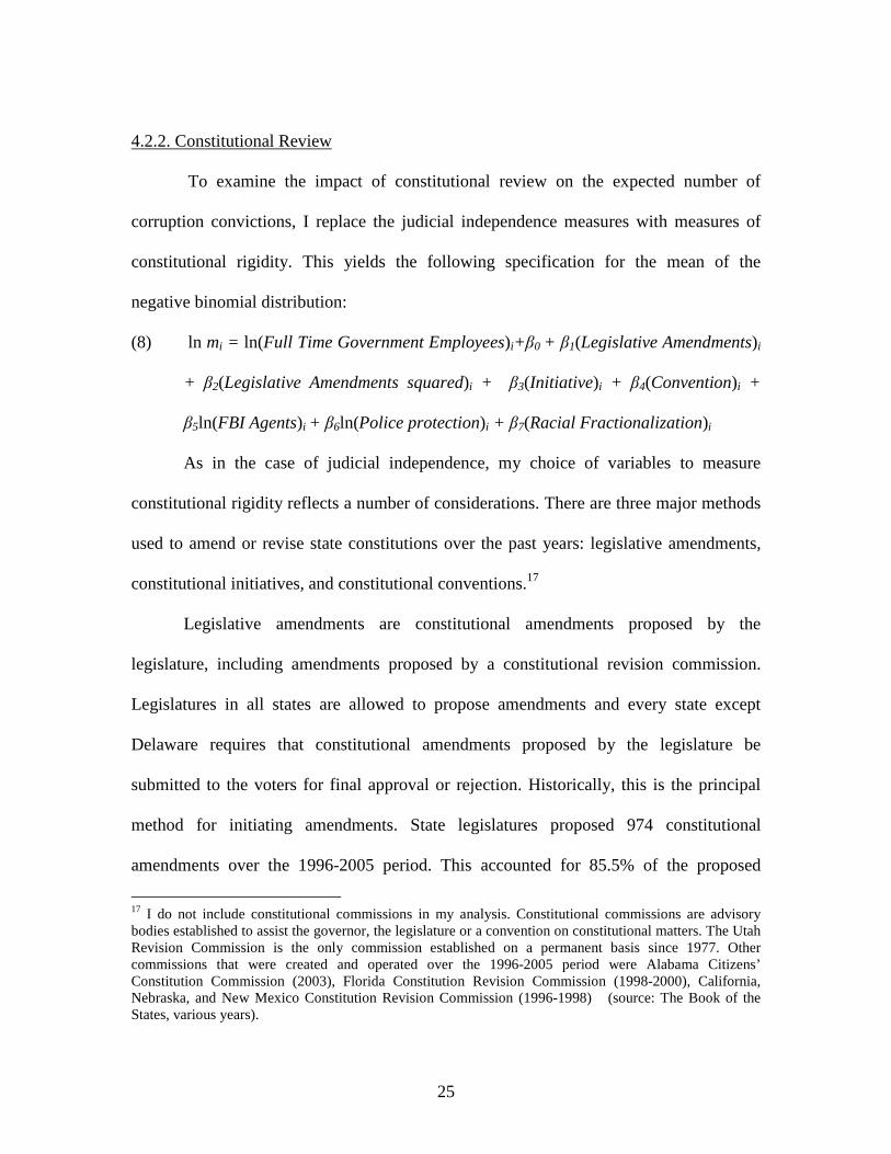
4.2.2. Constitutional Review
To examine the impact of constitutional review on the expected number of
corruption convictions, I replace the judicial independence measures with measures of
constitutional rigidity. This yields the following specification for the mean of the
negative binomial distribution:
(8) ln mi = ln(Full Time Government Employees)i+β0 + β1(Legislative Amendments)i
+ β2(Legislative Amendments squared)i + β3(Initiative)i + β4(Convention)i +
β5ln(FBI Agents)i + β6ln(Police protection)i + β7(Racial Fractionalization)i
As in the case of judicial independence, my choice of variables to measure
constitutional rigidity reflects a number of considerations. There are three major methods
used to amend or revise state constitutions over the past years: legislative amendments,
constitutional initiatives, and constitutional conventions.17
Legislative amendments are constitutional amendments proposed by the
legislature, including amendments proposed by a constitutional revision commission.
Legislatures in all states are allowed to propose amendments and every state except
Delaware requires that constitutional amendments proposed by the legislature be
submitted to the voters for final approval or rejection. Historically, this is the principal
method for initiating amendments. State legislatures proposed 974 constitutional
amendments over the 1996-2005 period. This accounted for 85.5% of the proposed
17 I do not include constitutional commissions in my analysis. Constitutional commissions are advisory bodies established to assist the governor, the legislature or a convention on constitutional matters. The Utah Revision Commission is the only commission established on a permanent basis since 1977. Other commissions that were created and operated over the 1996-2005 period were Alabama Citizens’ Constitution Commission (2003), Florida Constitution Revision Commission (1998-2000), California, Nebraska, and New Mexico Constitution Revision Commission (1996-1998) (source: The Book of the States, various years).
26
constitutional changes and 90.8% of those adopted. I include in my model the variable
Legislative Amendments, which represents the percentage of votes required in the state
legislature to propose constitutional amendments. In states that make it less costly to
change the constitution, i.e., those which require simple majority as opposed to
supermajorities, legislatures are more likely to enact amendments that benefit themselves
or special interest groups. On this matter, Anderson et al. (1990, p. 90) write:
…although amending the constitution is more costly and time-consuming than enacting legislation, a constitutional provision generally provides a more durable form of protection to an interest group than is possible through simple legislative action.
Since in a checks and balances system the strength of the political majority would
be offset by judicial review I expect a negative relationship between the variable
Legislative Amendments, which is also a proxy for constitutional rigidity, and corruption.
However, I do not necessarily expect a linear relation between the percentage of
legislative votes that is required for proposing amendments and constitutional rigidity.
Any supermajority vote, such as 60% or 67% represents a much higher hurdle than a
simple majority vote, but there may be a diminishing marginal effect from requiring the
approval of more than 60% of the legislators. Therefore I include both this variable and
its square in the model to capture nonlinear effects.
The constitutional initiative process, available in 18 states, allows citizens to
propose amendments to the constitution, without the consent of their elected
representatives. Among the 18 states, 16 have the direct initiative and two (Massachusetts
and Mississippi) have the indirect initiative. The direct initiative allows a proposed

27
measure to be placed on the ballot after a specific number of signatures have been
obtained on a citizen petition, while the indirect initiative requires submitting the measure
to the legislature for a decision prior to placing it on the ballot.18
The importance of the initiatives process in the United States has been
documented in studies by Romer and Rosenthal (1979), who see initiatives as the key to
breaking the legislature’s monopoly on making policy proposals, which is likely to result
in different policy outcomes, Kalt and Zupan (1990), who argue that initiatives may
eliminate informational asymmetries between voters and their representatives, Matsusaka
(1992), who emphasizes that in the presence of information imperfections, initiatives can
lead to policy outcomes distinct from those the legislature would choose, and Matsusaka
(1995), who shows that states with initiatives reduce government spending, shift the
spending from state to local governments, and adopt revenue structures that are more
dependent on fees and less on taxes. In addition, Matsusaka (2004) finds that initiatives
serve the interests of the many rather than the few. He argues that (i) initiatives provide
voters with choices, hence they are not forced to accept the policies implemented by the
legislature, and (ii) even though interest groups and wealthy individuals rely on initiatives
to promote their interests, the ability of voters to sort out bad policies from good policies
overturns the balance in the favor of the majority. Similar to the judicial review, the
initiatives process provides a check on the legislature by allowing citizens to overturn
policies contrary to their interests. Therefore I expect a negative sign on Initiative.
18 This information comes from the Book of the States, 2006.

28
The constitutional convention is a method of drafting a new constitution or
revising an existing one. No convention has assembled during the period of time studied,
1996 through 2005. Specifically, the last convention convened in 1986, in Rhode Island.
The variable Convention is a dummy for the states that provide for conventions in the
constitution (40 states in total). Since the convention is a method for making
constitutional changes, states that provide for conventions have less rigid constitutions,
ceteris paribus. Therefore my hypothesis predicts that this variable should have a positive
effect on corruption.
The same set of control variables is used here as in the preceding model relating
corruption to judicial independence.
4.3. Data
The corruption data were obtained from the Department of Justice’s “Report to
Congress on the Activities and Operations of the Public Integrity Section.” I combine the
information published in the 1999-2005 reports to determine the total number of
convictions by state for a ten-year period, 1996-2005. The crimes that are investigated
and reported by the Public Integrity Section include election crimes such as vote fraud,
campaign-finance violations, and political shakedowns, conflicts of interest, such as
misconduct proscribed by one of the federal conflict of interest statutes, or obstruction of
justice. Table 1 and Table 2 present the ten states that have the most convictions and the
ten states with the least corruption convictions per state government employee and per

29
state resident, respectively, over the entire sample period. Descriptive statistics for all
variables are reported in Table 3.
Table 1. States with Most and Least Corruption Convictions per State Government Employee
Most Convictions Fewer Convictions
State Convictions per 1000 government employees
State Convictions per 1000
government employees North Dakota 1.390 Vermont 0.327 Louisiana 1.186 South Carolina 0.323 Hawaii 1.181 Colorado 0.301 Mississippi 1.096 Utah 0.292 Florida 0.979 Minnesota 0.237 Montana 0.978 Kansas 0.232 Pennsylvania 0.968 New Hampshire 0.221 Kentucky 0.944 Iowa 0.153 Illinois 0.916 Oregon 0.107 Ohio 0.893 Nebraska 0.100 Note: Total corruption convictions over the years 1996-2005 per 1,000 full time government employees.
Table 2. States with Most and Least Corruption Convictions per State Resident
Most Convictions Fewer Convictions
State Convictions per 100,000 residents
State Convictions per 100,000 residents
North Dakota 0.845 South Carolina 0.189 Louisiana 0.735 Washington 0.173 Mississippi 0.711 Colorado 0.156 Hawaii 0.648 Utah 0.153 Alaska 0.605 Kansas 0.148 Montana 0.573 Minnesota 0.132 Kentucky 0.518 New Hampshire 0.110 South Dakota 0.491 Iowa 0.092 Florida 0.472 Nebraska 0.063 Ohio 0.469 Oregon 0.054 Note: Total corruption convictions over the years 1996-2005 per 100,000 state residents.
30
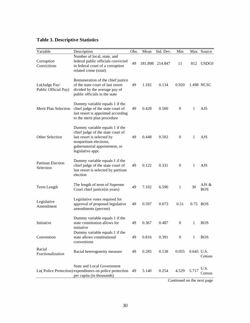
Table 3. Descriptive Statistics
Variable Description Obs. Mean Std. Dev. Min Max Source
Corruption Convictions
Number of local, state, and federal public officials convicted in federal court of a corruption related crime (total)
49 181.898 214.847 11 812 USDOJ
Ln(Judge Pay/ Public Official Pay)
Remuneration of the chief justice of the state court of last resort divided by the average pay of public officials in the state
49 1.182 0.134 0.920 1.498 NCSC
Merit Plan Selection
Dummy variable equals 1 if the chief judge of the state court of last resort is appointed according to the merit plan procedure
49 0.428 0.500 0 1 AJS
Other Selection
Dummy variable equals 1 if the chief judge of the state court of last resort is selected by nonpartisan elections, gubernatorial appointment, or legislative appt.
49 0.448 0.502 0 1 AJS
Partisan Election Selection
Dummy variable equals 1 if the chief judge of the state court of last resort is selected by partisan election
49 0.122 0.331 0 1 AJS
Term Length The length of term of Supreme Court chief justice(in years)
49 7.102 6.596 1 30 AJS & BOS
Legislative Amendment
Legislative votes required for approval of proposed legislative amendments (percent)
49 0.597 0.073 0.51 0.75 BOS
Initiative Dummy variable equals 1 if the state constitution allows for initiative
49 0.367 0.487 0 1 BOS
Convention Dummy variable equals 1 if the state allows constitutional conventions
49 0.816 0.391 0 1 BOS
Racial Fractionalization
Racial heterogeneity measure 49 0.285 0.138 0.055 0.645 U.S. Census
Ln( Police Protection) State and Local Government expenditures on police protection per capita (in thousands)
49 5.140 0.254 4.529 5.717 U.S. Census
Continued on the next page

31
Table 3 (continued)
Variable Description Obs. Mean Std. Dev. Min Max Source
Ln(FBI agents) Number of FBI agents per 100,000 residents, by state
49 3.125 0.549 1.722 4.309 US D.O.J.
Full-time Government Employees
Number of full time government employees, by state
49 305205.6 324463 35725.7 1671374 U.S. Census
Population Population by state, in thousands
49 5731.391 6277.93 496.437 34180.87 U.S. Census
Northeast Region Dummy variable equals 1 for the states in the Northeast region of US
49 0.204 0.407 0 1 U.S. Census
Ln(GSP per capita) Gross State Product per capita
49 10.382 0.171 10.026 10.856 U.S. Census
High School Percent state residents who completed high school or more
49 83.749 4.076 76.057 90.285 U.S. Census
Urban Population Percent state residents who live in urban area
49 71.625 15.051 38.179 94.443 U.S. Census
Percent 65 or older Percent state residents with the age of 65 or older
49 12.641 1.888 5.283 17.703 U.S. Census
Unemployment Rate Unemployment rate 49 4.691 0.868 2.91 7.02 U.S. Census
Note: Data are averaged over the years 1996 – 2005. USDOJ: United States Department of Justice NCSC: National Center of State Courts AJS: American Judicature Society BOS: The Book of the States
The main focus of the econometric model is on the existence of significant
relationships between corruption and (i) the variables that measure the degree of judicial
independence, or (ii) the measures of constitutional rigidity. Since the independent
variables exhibit little variation over time, I use the average of these variables over the
period 1996-2005. The dependent variable is total corruption convictions during the same

32
period. I use total rather than average corruption convictions to avoid having to deal with
fractional values in the negative binomial model. This is innocuous since averaging the
dependent variable would only change the magnitude of the coefficients, not their
statistical significance.
Figure 1 and 2 present histograms of the number of corruption convictions. The
data are strongly skewed to the right, thus OLS regressions are clearly inappropriate.
0.0
2.0
4.0
6.0
8D
ensi
ty
0 50 100 150Corruption convictions
Figure 1. Distribution of corruption convictions (490 observations from 1996-2005).
0.0
02.0
04.0
06D
ensi
ty
0 200 400 600 800corruptconvictions1
Figure 2. Distribution of corruption convictions (49 observations. Averaged values over 1996-2005).

33
Since I am examining count data, it might seem natural to start by fitting a
Poisson model. However, this model has the property of equidispersion (equality of mean
and variance). Table 4, which presents a detailed description of the dependent variable,
shows that the variance of the Corruption Convictions variable is about 255 times greater
than the mean. This leads me to believe that the Poisson model is inappropriate.
Table 4. Detailed Description of the Corruption Convictions Variable
Corruption convictions (totals by state) Percentiles Smallest
1% 11 11 5% 14 12
10% 19 14 Obs. 49 25% 40 19 Sum of Wgt. 49 50% 95 Largest Mean 181.898 75% 209 570 Std. Dev. 214.8472 90% 569 759 Variance 46159.3 95% 759 793 Skewness 1.721 99% 812 812 Kurtosis 4.938
To reinforce this argument, I perform a test for overdispersion by estimating an
auxiliary regression (Cameron and Trivedi 2005, p.671) and conducting a one-sided t-test
for the slope coefficient. The results, which are reported in Table 5, reject the equality of
the mean and variance. In Figure 3, I graph the Corruption Convictions variable against a
Poisson distribution with the same mean and a Negative Binomial distribution with the
same mean and variance. The negative binomial distribution is clearly a better fit to the
data.

34
Table 5. Test of Overdispersion
Z_Corruption OLS regression, no constant Lambda_Corruption 1.754***
(3.06) F-statistic 9.38
49 Number of Observations Notes: The null hypothesis is no overdispersion. I test this hypothesis by estimating an auxiliary simple regression model with no intercept. The dependent variable is ((Yi-µ_hati)^2-Yi)/µ_hati and the independent variable is µ_hati . No overdispersion implies that the slope coefficient is zero. I report the estimated slope and the t-statistic for the one-sided test in parentheses. *** indicates significant at the 1 % level. Lambda_Corruption (µ_hati) represents the estimates of the variance of the dependent variable, Corruption Convictions (Yi), after fitting the model using a Poisson regression. Z_corruption was constructed as ((Yi-µ_hati)^2-Yi)/µ_hati.
0.0
2.0
4.0
6.0
8.1
Pro
port
ion
0 2 4 6 8 10Corruption convictions
observed proportion neg binom probpoisson prob
mean = 18.19; overdispersion = 1.426
Note: 490 observations over 1996-2005.
Figure 3. Observed number of corruption convictions against a Poisson distribution with the same mean and a Negative Binomial distribution with the same mean and variance.
Based on the above arguments and for reasons detailed in section 4.1, I conduct
my analysis using a generalized negative binomial model. This is just a generalization of
the negative binomial regression which allows the variance of the dependent variable to
be a function of explanatory variables. The corruption data come from four different
regions of the United States (Northeast, Midwest, South, and West). Since these regions
35
differ among themselves in many aspects, and especially on the basis of population
density, it is reasonable to believe that the variance could be different depending on the
region. To allow for this possibility I investigated specifications in which the variance of
the dependent variable is explained by regional dummies. Based on the estimation results,
it appears that the Northeast region has a substantially lower variance than the other
regions (the coefficients for the other regions are not statistically significant). Therefore I
include a Northeast dummy in the variance equation for all models considered.
4.4. Estimation Results
4.4.1. Judicial Independence
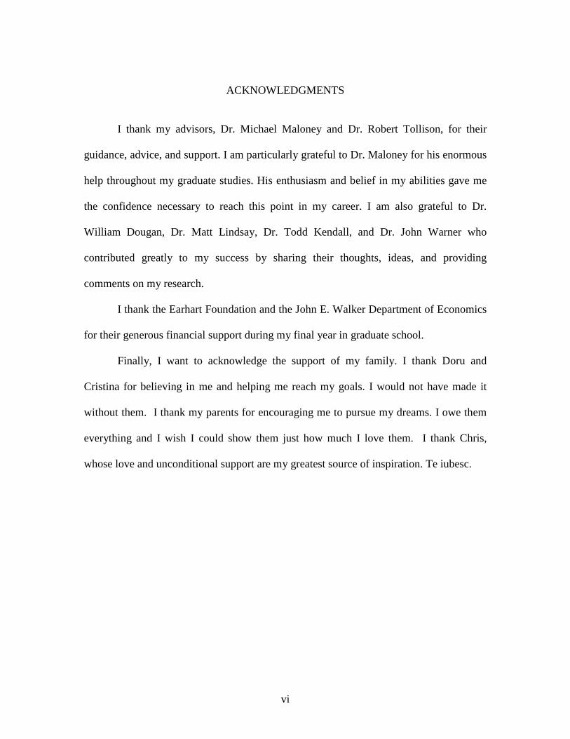
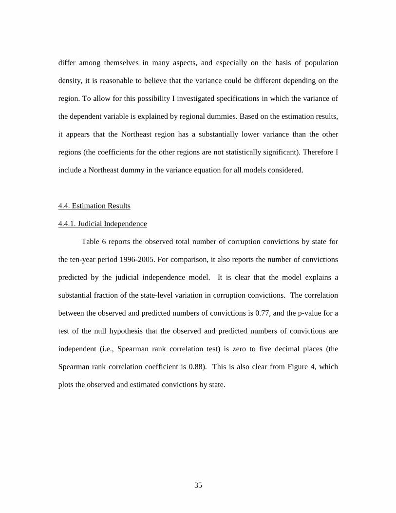
Table 6 reports the observed total number of corruption convictions by state for
the ten-year period 1996-2005. For comparison, it also reports the number of convictions
predicted by the judicial independence model. It is clear that the model explains a
substantial fraction of the state-level variation in corruption convictions. The correlation
between the observed and predicted numbers of convictions is 0.77, and the p-value for a
test of the null hypothesis that the observed and predicted numbers of convictions are
independent (i.e., Spearman rank correlation test) is zero to five decimal places (the
Spearman rank correlation coefficient is 0.88). This is also clear from Figure 4, which
plots the observed and estimated convictions by state.

36
Table 6. Observed and Predicted Number of Corruption Convictions
State Observed
Convictions Predicted
Convictions State
Observed Convictions
Predicted Convictions
Alabama 177 218 Montana 52 35 Alaska 38 55 Nebraska 11 33 Arizona 106 131 Nevada 46 69 Arkansas 68 59 New Hampshire 14 17 California 812 1327 New Jersey 371 346 Colorado 70 137 New York 793 806 Connecticut 92 87 North Carolina 156 278 Delaware 33 18 North Dakota 54 26 Florida 759 276 Ohio 533 261 Georgia 217 240 Oklahoma 95 98 Hawaii 81 96 Oregon 19 114 Idaho 43 30 Pennsylvania 528 523 Illinois 569 611 Rhode Island 25 20 Indiana 125 98 South Carolina 76 142 Iowa 27 39 South Dakota 37 17 Kansas 40 59 Tennessee 206 112 Kentucky 210 86 Texas 570 1797 Louisiana 328 393 Utah 35 38 Maine 27 29 Vermont 12 14 Maryland 105 228 Virginia 235 267 Massachusetts 178 178 Washington 103 206 Michigan 209 231 West Virginia 69 92 Minnesota 65 137 Wisconsin 109 119 Mississippi 202 119 Wyoming 19 15 Missouri 164 100 Notes: Average observed number of corruption convictions over 1996-2005 vs. number of corruption convictions predicted by the generalized negative binomial model with judicial independence measures. The correlation between observed and predicted numbers of convictions is 0.77. The p-value for a test of the null hypothesis that the observed and the predicted number of convictions are independent (i.e., Spearman rank correlation test) is zero to five decimal places. The Spearman rank correlation coefficient is 0.88.
37
050
010
0015
0020
00
1 3 5 7 9 11 13 15 17 19 21 23 25 27 29 31 33 35 37 39 41 43 45 47 49stateid
corruptconvictions1 predicted number of events
Note: 49 observations. Averaged values over 1996-2005.
Figure 4. Observed number of corruption convictions and number of convictions predicted by the Generalized Negative Binomial model, by state.
Next, consider the estimation results for the judicial independence model
presented in Table 7. In general, the results are consistent with my hypothesis that states
where judges are more independent experience lower levels of corruption. The estimated
coefficients for Judge Pay/Public Official Pay, Merit Selection and Other Selection have
the correct sign and they are all statistically different from zero at the 1% significance
level. The variable Term Length also has the correct sign but is not significant at standard
levels.
For the variables that are statistically significant, the marginal effects are
substantial. First consider the two dummy variables, Merit Plan Selection and Other
Selection. The estimates indicate that replacing the partisan election method of selecting
judges with the merit plan method would decrease the number of corruption convictions
by approximately 95 over a ten-year period. Similarly, a change from a partisan election
selection method to nonpartisan election, gubernatorial or legislative appointment would

38
decrease the number of corruption convictions by approximately 75 over a ten-year
period. Second, if the ratio of judge pay to public official pay increases by 10% the
expected number of corruption convictions decreases by approximately 18.4 over a ten-
year period.
The results with respect to the controls for law enforcement effectiveness are
mixed. The coefficient on the variable measuring state and local expenditures on police
protection per capita has a negative sign but is not statistically significant. The
coefficient on the variable FBI agents is significant at the 5% significance level and has a
positive sign.
Although the Racial Fractionalization variable does not play a role in my
hypothesis the coefficient has the sign expected based on the results of previous studies,
suggesting that by increasing racial heterogeneity by one percentage point the number of
corruption convictions increases by approximately 2.3 over a ten-year period.
4.4.2. Constitutional Rigidity
Now consider the results on constitutional review presented in Table 8. Once
again the results are consistent with my hypothesis that states with more rigid
constitutions should experience less corruption. The coefficients for the variable
Legislative Amendments and its square are both significant at the 1% level. Legislative
Amendment has a negative sign and its square has a positive sign. To properly interpret
this finding I need to look at the combined effect of these variables on predicted
corruption levels. The combined effect implies that as the required percentage of votes
for approval of amendments increases, corruption decreases. Most of this effect is

39
attributable to the change from a simple majority to a supermajority of 60%. The effect of
going from a supermajority of 60% to one of 67% is not nearly as large.
The coefficient on the dummy variable for Initiative is significant at the 1% level
and has the predicted sign. The estimate indicates that changing the constitution to allow
for voter initiatives should reduce the number of corruption convictions by approximately
24 over a ten-year period. The coefficient on the dummy variable for Convention is also
significant at the 1% level. Its sign is not as predicted, however. According to my
hypothesis, a more rigid constitution should reduce corruption, which corresponds to a
positive sign on the Convention variable. The negative sign may indicate that the
provision for constitutional convention actually acts as a check on the power of
legislature. Susan Rose-Ackerman (1999) mentions the importance of the public as a
check on the arbitrary exercise of power by the government. In 14 of the 40 states that
allow conventions, voters can reject a convention call. It follows that in order to issue a
successful convention call, the amendments brought to the constitution have to benefit
the majority of voters.
The results for the law enforcement variables are similar to those reported in
Table 7. The estimated coefficients on the variable FBI agents and on the variable
measuring state and local expenditures on police protection have the same signs as before
and are statistically significant at the 10% level and the 1% level, respectively. Also, the
estimated coefficient for the control variable Racial Fractionalization is positive and
significant at the 1% level, as expected.

40
Table 7. Effect of Judicial Independence on Corruption in the United States
Dependent Variable Variables Corruption Convictions Generalized Negative Binomial
Exposure variable Full Time
Government Employees
Coeff.
(z) Marginal Effects
(dy/dx) Ln(Judge Pay/Public Official Pay) -1.722*** -184.546*** (-3.57) (-3.43) Merit Plan Selection -0.915*** -95.085*** (-10.02) (-11.62) Other Selection Procedure -0.714*** -75.395*** (-9.12) (-9.61) Term Length -0.001 -0.191 (-0.44) (-0.44) Ln(FBI Agents) 0.209** 22.494** (2.48) (2.40) Ln(Police Protection) -0.179 -19.207 (-0.61) (-0.60) Racial Fractionalization 2.139*** 229.281*** (3.19) (2.99) Constant -5.089*** - (-3.07) - lnalpha Northeast Region -13.707* - (-1.76) - Constant -1.154*** - (-4.72) - Log-likelihood -250.053 - LR chi2(7) 29.35 - Number of Observations 49 - Notes: {***, **,*} indicates significant at 1, 5, and 10 percent level, respectively.

41
Table 8. Effect of Constitutional Review on Corruption in the United States Dependent Variable Variables Corruption Convictions Generalized Negative Binomial
Exposure variable Full Time
Government Employees
Coeff.
(z) Marginal Effects
(dy/dx) Legislative Amendment -19.768*** -2220.682*** (-3.00) (-3.10) Legislative Amendment squared 15.589*** 1751.213*** (2.82) (2.91) Initiative -0.219*** -24.000*** (-3.53) (-3.53) Convention -0.404*** -52.015*** (-7.37) (-7.39) Ln(FBI Agents) 0.162* 18.212* (1.79) (1.79) Ln(Police Protection) -0.810*** -91.043** (-3.83) (-3.44) Racial Fractionalization 2.618*** 294.167*** (4.69) (4.33) Constant 2.026 - (0.89) - lnalpha Northeast Region -15.343*** - (-6.73) - Constant -1.112*** - (-4.58) - Log-likelihood -251.866 - LR chi2(7) 25.72 - Number of Observations 49 - Notes: {***, **,*} indicates significant at 1, 5, and 10 percent level, respectively.
42
4.5. Robustness
As a robustness check I fit both models a second time using state population as
the exposure variable rather than the number of full-time government employees. The
results are presented in Table 9, column 1, for the judicial independence model and Table
10, column 1, for the constitutional review model. In general, the results are very similar
to those reported in Table 7 and Table 8. To further address the robustness of my results,
in an unreported regression I fit the data by allowing the coefficient on the exposure
variable, full-time government employees, to vary from unity. This does not affect the
significance or the sign of the estimates.19
I also fit a single model that includes both measures of judicial independence and
measures of constitutional review. The downside of this estimation is that the number of
covariates is large relative to the sample size. Nonetheless, the variables measuring
judicial independence maintain their significance. Among the measures of constitutional
rigidity, only the convention variable has a statistically significant z-score. The p-value
for a test of the null hypothesis that all the judicial independence and constitutional
rigidity variables can be excluded from the model is zero to five decimals places, while
the p-values for tests that exclude only the judicial independence measures or only the
constitutional rigidity measures are 0.006 and 0.039, respectively. This confirms the
robustness of the general findings from the separate models.
Some might wonder whether my findings regarding the relation between judicial
independence and corruption are indicative of a more general relation between judicial
19 The estimated coefficient for ln(full time government employees) is -0.123 (with a z-score of -1.73) for the judicial independence model and 0.049 (with a z-score of 0.97) for the constitutional review model.

43
independence and crime. To investigate this hypothesis, I estimated linear regressions
with crime rate per capita as the dependent variable and the same independent variables
that entered the negative binomial regressions. The results of this analysis look very
different from those using corruption as dependent variable, with little evidence of a
statistically significant relation between crime rates and any of the judicial independence
or constitutional rigidity measures. The one variable that is consistently significant is
racial fractionalization.
A general source of concern in analyzing count data is the existence of excess
zeros. However, Table 4 shows that there are no values of zero for my dependent
variable, Corruption Convictions. In fact, looking at the dataset by years from 1996-2005,
the variable Corruption Conviction has the value of zero only in about 8 % of the data.
Another potential concern is that corruption and judicial independence or
constitutional review are determined by factors omitted from the model and thus my
estimates are the result of spurious correlation. To assess the impact of including
additional controls, I ran all the regressions again with variables added to account for the
levels of income, education, and unemployment by state, as well as for the percentage of
state residents that live in an urban area and are 65 years or older. Earlier studies, such as
Glaeser and Saks (2004), Meier and Holbrook (1992), have found these variables to have
significant effects on corruption levels across states. The inclusion of these control
variables does not affect the significance of my results. These results are reported in
Table 9, columns 2 and 3, for the judicial independence model, and Table 10, columns 2
and 3, for the constitutional review model.

44
Table 9. Effect of Judicial Independence on Corruption: Robustness Check
Dependent Variable Variables Corruption Convictions Generalized Negative Binomial
Exposure variable State
Population Full Time
Government Employees [1] [2] [3]
Coeff.
(z) Coeff.
(z) Coeff.
(z) Ln(Judge Pay/Public Official Pay) -1.817*** -1.317** -1.082** (-3.74) (-2.44) (-2.19) Merit Plan Selection -0.673*** -0.927*** -0.609*** (-7.35) (-9.40) (-5.21) Other Selection Procedure -0.543*** -0.627*** -0.427*** (-6.97) (-7.97) (-3.70) Term Length -0.001 -0.012*** -0.003 (-0.46) (-3.02) (-0.80) Ln(FBI Agents) 0.336*** 0.264*** 0.249*** (3.98) (2.77) (3.01) Ln(Police Protection) -0.229 0.151 -0.194 (-0.79) (0.60) (-0.71) Racial Fractionalization 2.358*** - 2.468*** (3.54) - (4.05) Ln(GSP per capita) - 0.825** - - (1.99) - High School - -0.062*** - - (-3.01) - Unemployment Rate - - -0.082 - - (-1.15) Percent 65 or older - - 0.109*** - - (3.51) Constant -1.381 -10.138*** -7.275*** (-0.83) (-2.65) (-4.66) lnalpha Northeast Region -20.823*** -17.355*** -35.279*** (>100) (-11.04) (>100) Constant -1.119*** -1.116*** -1.445*** (-4.60) (-4.57) (-5.99) Log-likelihood -250.927 -250.626 -242.350 LR chi2 30.77 28.20 44.75 Number of Observations 49 49 49 Notes: {***, **,*} indicates significance at 1, 5, and 10 percent level, respectively.

45
Table 10. Effect of Constitutional Review on Corruption: Robustness Check
Dependent Variable Variables Corruption Convictions Generalized Negative Binomial
Exposure variable State
Population Full Time
Government Employees [1] [2] [3]
Coeff.
(z) Coeff.
(z) Coeff.
(z) Legislative Amendment -13.096** -27.976*** -18.842** (-1.92) (-3.42) (-2.00) Legislative Amendment squared 10.376* 22.947*** 15.306** (1.80) (3.33) (1.92) Initiative -0.220*** -0.180*** -0.218*** (-3.50) (-2.74) (-3.32) Convention -0.297*** -0.512*** -0.361*** (-5.27) (-6.76) (-3.47) Ln(FBI Agents) 0.285*** 0.095 0.245** (3.26) (0.99) (1.96) Ln(Police Protection) -0.416** -0.107 -0.684 (-2.20) (-0.29) (-1.44) Racial Fractionalization 2.123*** 2.125*** 1.507*** (4.26) (3.50) (2.36) Ln(GSP per capita) - -0.873* -0.560 - (-1.97) (-0.98) High School - -0.007 - - (-0.37) - Unemployment Rate - - 0.093 - - (1.06) Urban Population - - 0.011* - - (1.83) Constant 1.501 10.754** 5.460 (0.67) (2.24) (0.83) lnalpha Northeast Region -18.140*** -16.715*** -16.568*** (-30.92) (-23.26) (-13.41) Constant -1.212*** -1.186*** -1.206*** (-5.13) (-4.93) (-5.11) Log-likelihood -248.446 -249.662 -247.634 LR chi2 35.73 30.13 34.19 Number of Observations 49 49 49 Notes: {***, **,*} indicates significance at 1, 5, and 10 percent level, respectively.

46
Of course, it always possible that other unobserved factors account for the relation
between corruption and the judicial independence and constitutional rigidity measures.
The measures might be correlated with policies that reduce corruption, they might reflect
endogenous selection of public officials into different states, or they might be affected by
the level of corruption. If this is the case, then it does not necessarily follow that
increasing judicial independence and constitutional rigidity will reduce corruption.
Nonetheless, my results suggest that investigating whether we can deter corruption by
promoting judicial independence would be a worthwhile policy endeavor.
4.6. Conclusions
In the United States system of government, judicial oversight provides an
important check on the abuse of power by the legislative and executive branches. I
investigate whether two distinct components of the oversight function — judicial
independence and constitutional rigidity — are related to a specific type of abuse of
power by government officials: corruption in public office. Specifically, I use data for 49
states over 1996-2005 to develop measures of judicial independence and constitutional
rigidity and examine their impact on corruption convictions.
Unlike previous studies, I develop an econometric specification that recognizes
the distinction between the observed number of convictions for corruption and the
unobserved number of corrupt officials. I show that by including variables that pick up
differences in law enforcement effectiveness across states, I should be able to use
convictions data to draw valid inferences about the underlying level of corruption. In

47
general, I find that both judicial independence and constitutional rigidity are significant
predictors of corruption. First, in states where judges have a greater degree of
independence (higher remuneration, merit plan selection, or longer terms), there is less
corruption. Second, in states that have more rigid constitutions (larger legislative
majorities required to propose constitutional amendments), there is less corruption.
These findings complement existing evidence from cross-country studies that judicial
independence and constitutional review are predictors of freedom.
The policy implications of my analysis are relatively straightforward. There is
mounting evidence from the international arena that high levels of corruption limit
investment, retard economic growth, lead to ineffective government, and create economic
inefficiencies and inequalities. My findings suggest that constitutional and judicial
reform could play a significant role in reducing the prevalence of corruption in
developing economies around the world. This conclusion is tentative, however, because
of endogeneity concerns. Further work will be required to establish firm
recommendations in this regard. The next chapter, which provides evidence on the
relation between corruption, judicial independence, and constitutional rigidity using
country-level data, is intended as a first step in this process.

48
CHAPTER FIVE
EVIDENCE FROM ACROSS COUNTRIES
Researchers do not have many options when deciding how to measure corruption
at the country level. There is no international database of convictions for corruption by
country. As a result, the literature relies on survey-based measures. There are, however,
several different sources of corruption indicators. Rather than choose one indicator, I
examine the three indicators that are used most frequently in other studies.
5.1. Empirical Specifications
Transparency International, the World Bank, and the Political Risk Service Group
are the three main sources of country-level corruption data. Each organization publishes
an index that provides a rank ordering of countries from least to most corrupt. The exact
methodology used to construct the index varies from one organization to another. I
provide the details after discussing the empirical specifications. Like most of the
literature, I use linear regression methods to investigate differences in corruption across
countries. Since data availability varies across indices, I conduct my analysis on cross-
sections of between 37 to 165 countries for various years between 1995 and 2005. I then
extend my analysis to panels of data with cross-sectional and time-series observations for
1998 to 2005.
5.1.1. Judicial Independence
To examine the effect of judicial independence on corruption in a cross section of
countries, I estimate the following regression models:

49
(1) Corruptioni= β0 + β1(Judicial Independence)i + β2ln(GDP per capita)i +
β3(Education Index)i + β4(Percent Protestant)i + β5(Ethnic Fractionalization)i +εi
(2) Corruptioni= β0 + β1(Judicial Independence)i + β2ln(GDP per capita)i +
β3(Education Index)i + β4(Percent Protestant)i + β5(Ethnic Fractionalization)i +
β6ln(Government Size)i + β7(Common Law)i + β8(Developing Country)i + εi
I consider three measures of judicial independence: two survey-based indices
derived from the Economic Freedom of the World Report published by the Fraser
Institute and from the Political Constraint Index Dataset, and an index based on the legal
foundations as found in the legal documents of a country, constructed by La Porta et al.
(2004).
My choice of control variables is based on the previous literature on the
determinants of corruption. Even though there is no commonly agreed upon empirical
model to explain corruption, previous studies, such as La Porta et al. (1999), Treisman
(2000), Adsera et al. (2000), Lederman et al. (2001), La Porta et al. (2004), and Waisman
(2005), almost always include economic, cultural, and socio-demographic variables in
their analysis. I follow the literature and account for the robustness of my estimation by
controlling for a number of country characteristics.
The first three controls measure the impact of economic development: the log of
the gross domestic product per capita, an education index and a dummy variable for
developing countries. In general, previous studies (Treisman, 2000, Waisman, 2005)
argue that developing countries are more affected by corruption than developed ones, and

50
that richer and more educated societies have lower levels of corruption as more educated
and richer voters are more willing and able to monitor and expose public officials when
they violate the law.
The fourth control measures the percentage of the country’s population that is
from a Protestant tradition. Previous studies suggest that a country’s religious tradition
might influence the costs of corrupt activities. According to La Porta (1999), Protestant
countries, as opposed to Catholic or Muslim countries, are less interventionist and should
display better government performance due to higher ethical standards of politicians in
office.
The fifth control is a measure of ethnic divisions within a country. The literature
suggests that ethnic heterogeneity increases corruption or reduces people's desire to
oppose corruption. In ethnically heterogeneous societies, there are more opportunities for
redistribution within the group that comes to power, which is often interested in adopting
policies to restrict the freedom of those outside the ruling group, and to limit the
production of public goods (La Porta et al., 1999). Thus, if a political leader allocates
resources to the ethnic group to which he belongs, members of that ethnic group continue
to support him, even though he is corrupt (Glaeser and Saks, 2004).
The sixth control is a measure of government size. Government size has an
ambiguous effect on corruption. On the one hand, larger governments may imply (i)
lesser bureaucratic delay, thus less rent-seeking, and (ii) higher wages for public officials,
thus lower incentives to accept bribes. On the other hand, larger governments suggest
more inefficiencies and opportunities for rent-seeking.

51
The seventh control is a dummy variable for countries with a common law legal
system. The idea is that the effectiveness of a country’s legal system affects the
probability of getting caught and convicted of corruption. La Porta et al. (1999) suggest
that common law systems, as opposed to civil law systems, offer a greater protection of
property rights and are more effective due to the willingness of judges to follow
procedures, which increases the chances of exposing corruption.
To further check the robustness of my results, I include three other control
variables in the panel data specifications: the log of investment as share of the gross
domestic product, an index of freedom of the press, and a dummy variable for countries
with a federal structure. Higher investment leads to economic development and thus less
corruption. Press freedom is important as it results in better informed voters and
improved transparency, thus increasing the accountability of public officials. The effect
of the federal structure on corruption could go in either direction. Some argue that
competition between jurisdictions leads to more honest and efficient government
(Weingast, 1995), while others suggest that there are greater opportunities for corruption
in a decentralized political system because one needs to influence only one segment of
the government or because there is more interaction between private individuals and
public officials (Banfield, 1979).
5.1.2. Constitutional Review
To examine the effect of constitutional review on corruption, I replace the judicial
independence measure with an index of constitutional review. This yields the following
regression models:
52
(3) Corruptioni= β0 + β1(Constitutional Review)i + β2ln(GDP per capita)i +
β3(Education Index)i + β4(Percent Protestant)i + β5(Ethnic Fractionalization)i+εi
(4) Corruptioni= β0 + β1(Constitutional Review)i + β2ln(GDP per capita)i +
β3(Education Index)i + β4(Percent Protestant)i + β5(Ethnic Fractionalization)i +
β6ln(Government Size)i + β7(Developing Country)i + εi
My measure of constitutional review is an index created by La Porta et al. (2004).
The set of control variables used in the preceding models relating judicial independence
to corruption is used here as well.
5.2. Data
As noted earlier, the literature on corruption at the country level relies on indices
of “perceived” corruption, which are almost always criticized for being subjective.
However, as Treisman (2000) points out, the various organizations that administer
surveys to construct cross-country ratings of corruption use very different methodologies
and, still, the indices derived are highly correlated, suggesting that they do measure
something very similar. Table 11 presents the correlations between the three corruption
indicators used in my analysis: the Corruption Perceptions Index compiled by
Transparency International (Corruption TI), the Control of Corruption Index compiled by
researchers at the World Bank (Kaufman et al., 2007) (Corruption World Bank), and the
International Country Risk Guide (ICRG) Corruption Index compiled by the Political
Risk Survey Group (Corruption PRS).

53
Table 11. Correlation Coefficients between Corruption Indicators
Corruption TI Corruption World Bank Corruption PRS Corruption TI 1.000 - - Corruption World Bank 0.965 1.000 - Corruption PRS 0.824 0.822 1.000
The main corruption indicator, Corruption TI, provides data on extensive
perceptions of corruption within countries. It is a composite index, computed as the
average of surveys from up to 14 sources originating from 12 independent institutions.
These surveys are based on the views of business people, risk analysts, journalists, and
the general public, and contain questions about the "spread and amount of corruption in
public and private business, the likeliness to demand special and illegal payments in high
and low levels of government, the degree of misuse of public power for private benefits,
the frequency of cases of corruption for politicians, public officials, policemen, and
judges, or improper practices, such as bribing or corruption, in the public sphere,” etc.20
This index ranges from zero (highly corrupt) to 10 (highly clean). I reversed the scale to
range from zero (highly clean) to 10 (highly corrupt). Table 12 ranks the ten most corrupt
and the ten least corrupt countries based on this index. According to Corruption TI, the
least corrupt country in my sample is Denmark, with an average score of 0.38, and the
most corrupt is Bangladesh, with a score of 8.52. The United States has an average score
of 2.41.
20 A detailed description of the methodology for the Corruption Perceptions Index is available at: http://www.transparency.org/policy_research/surveys_indices/cpi.
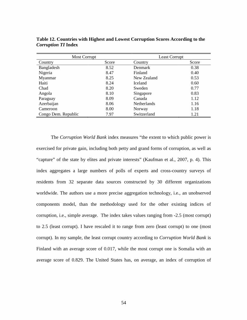
54
Table 12. Countries with Highest and Lowest Corruption Scores According to the Corruption TI Index
Most Corrupt Least Corrupt Country Score Country Score Bangladesh 8.52 Denmark 0.38 Nigeria 8.47 Finland 0.40 Myanmar 8.25 New Zealand 0.53 Haiti 8.24 Iceland 0.60 Chad 8.20 Sweden 0.77 Angola 8.10 Singapore 0.83 Paraguay 8.09 Canada 1.12 Azerbaijan 8.06 Netherlands 1.16 Cameroon 8.00 Norway 1.18 Congo Dem. Republic 7.97 Switzerland 1.21
The Corruption World Bank index measures “the extent to which public power is
exercised for private gain, including both petty and grand forms of corruption, as well as
“capture” of the state by elites and private interests” (Kaufman et al., 2007, p. 4). This
index aggregates a large numbers of polls of experts and cross-country surveys of
residents from 32 separate data sources constructed by 30 different organizations
worldwide. The authors use a more precise aggregation technology, i.e., an unobserved
components model, than the methodology used for the other existing indices of
corruption, i.e., simple average. The index takes values ranging from -2.5 (most corrupt)
to 2.5 (least corrupt). I have rescaled it to range from zero (least corrupt) to one (most
corrupt). In my sample, the least corrupt country according to Corruption World Bank is
Finland with an average score of 0.017, while the most corrupt one is Somalia with an
average score of 0.829. The United States has, on average, an index of corruption of
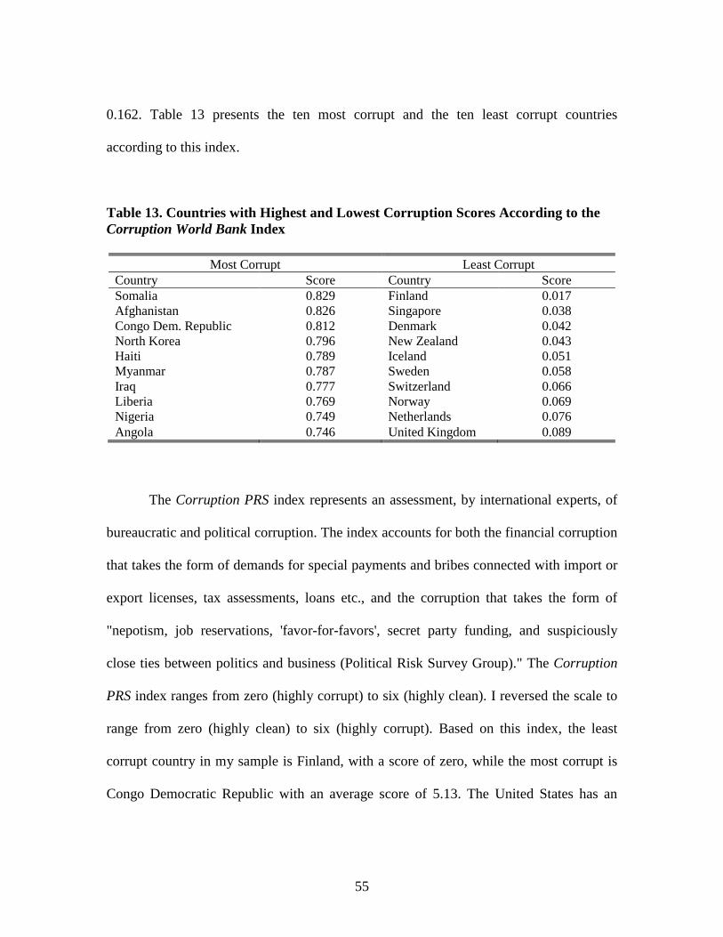
55
0.162. Table 13 presents the ten most corrupt and the ten least corrupt countries
according to this index.
Table 13. Countries with Highest and Lowest Corruption Scores According to the Corruption World Bank Index
Most Corrupt Least Corrupt Country Score Country Score Somalia 0.829 Finland 0.017 Afghanistan 0.826 Singapore 0.038 Congo Dem. Republic 0.812 Denmark 0.042 North Korea 0.796 New Zealand 0.043 Haiti 0.789 Iceland 0.051 Myanmar 0.787 Sweden 0.058 Iraq 0.777 Switzerland 0.066 Liberia 0.769 Norway 0.069 Nigeria 0.749 Netherlands 0.076 Angola 0.746 United Kingdom 0.089
The Corruption PRS index represents an assessment, by international experts, of
bureaucratic and political corruption. The index accounts for both the financial corruption
that takes the form of demands for special payments and bribes connected with import or
export licenses, tax assessments, loans etc., and the corruption that takes the form of
"nepotism, job reservations, 'favor-for-favors', secret party funding, and suspiciously
close ties between politics and business (Political Risk Survey Group)." The Corruption
PRS index ranges from zero (highly corrupt) to six (highly clean). I reversed the scale to
range from zero (highly clean) to six (highly corrupt). Based on this index, the least
corrupt country in my sample is Finland, with a score of zero, while the most corrupt is
Congo Democratic Republic with an average score of 5.13. The United States has an

56
average score of 1.78. Table 14 ranks the ten most corrupt and the ten least corrupt
countries based on this index.
Table 14. Countries with Highest and Lowest Corruption Scores According to the Corruption PRS Index
Most Corrupt Least Corrupt Country Score Country Score Congo Dem. Republic 5.13 Finland 0.00 Somalia 5.00 Sweden 0.12 Niger 4.93 Denmark 0.17 Sudan 4.79 Netherlands 0.24 Myanmar 4.79 Iceland 0.28 Iraq 4.79 Canada 0.35 Nigeria 4.61 New Zealand 0.71 Liberia 4.36 Luxembourg 0.75 Russia 4.34 Norway 0.83 Zimbabwe 4.33 Switzerland 0.95
To measure the level of judicial independence across countries I use three types of
indicators. I report the correlations between these indicators in Table 15.
Table 15. Correlation Coefficients between Judicial Independence Indicators
Judicial
Independence (I) Judicial
Independence (II) Judicial
Independence (III) Judicial Independence (I) 1.000 - - Judicial Independence (II) 0.573 1.000 - Judicial Independence (III) 0.396 0.408 1.000
The main judicial independence variable, Judicial Independence (I), was
compiled by the World Economic Forum Organization, and published in the Economic

57
Freedom of the World Report by the Fraser Institute. This measure is based on the World
Economic Forum’s annual Executive Opinion Survey whose goal is to obtain accurate
information about country specific attributes that are not well recorded in quantitative
sources. The respondents to the Survey are typically a company’s CEO or a member of
its senior management. This Survey provides the basis for a comparative assessment on a
global basis, this being facilitated by interviewing a large number of senior business
leaders and by ensuring that the sample in each country is not biased in favor of any
particular business group. Moreover, to check their consistency, the survey responses are
compared to hard data, when available, which shows that the quantitative sources and the
Survey results are positively correlated.
The Judicial Independence (I) index is based on the following question: “Is the
judiciary in your country independent from political influences of members of
government, citizens, or firms? (1 = no – heavily influenced, 7 = yes – entirely
independent).” The question’s wording has varied slightly over the years. The index has
been rescaled to range from zero (heavily influenced judiciary) to 10 (entirely
independent judiciary). Table 16 reports the ten countries with the highest and lowest
levels of judicial independence, respectively. According to Judicial Independence (I), in
my sample, the country with the most independent judiciary is Finland, with an average
score of 9.1, while the country with the least independent judiciary is Haiti, with an
average score of 0.2. The United States has an average score of 7.6.

58
Table 16. Countries with Most and Least Independent Judiciaries According to Judicial Independence (I) Index
Most Independent Least Independent Country Score Country Score Finland 9.1 Haiti 0.2 Denmark 9.0 Nicaragua 0.8 Netherlands 9.0 Venezuela 1.0 Germany 9.0 Paraguay 1.1 Australia 8.9 Burundi 1.3 New Zealand 8.9 Chad 1.4 United Kingdom 8.7 Ecuador 1.4 Switzerland 8.5 Kyrgyzstan 1.5 Norway 8.5 Bolivia 1.8 Israel 8.5 Peru 1.9
The next judicial independence measure, Judicial Independence (II), comes from
the Political Constraint Index Dataset21 (POLCON). POLCON defines the existence of an
independent judiciary by the joint existence of a POLITY score on executive constraints
(XCONST) of at least three, i.e., slight to moderate limitations on the executive authority,
and an ICRG score on Law and Order of at least four, i.e., a relatively strong law and
order tradition. As noted in the POLCON Codebook (Henisz, 2005), the variable
XCONST refers to “the extent of institutionalized constraints on the decision-making
powers of chief executives. Such limitations may be imposed by any accountability
groups. In Western democracies these are usually legislatures. Other kinds of
accountability groups are the ruling party in a one-party state […] and, in many states, a
strong, independent judiciary. The concern is therefore with the checks and balances
between the various parts of the decision-making process.” Slight to moderate limitations
21 The POLCON Dataset is available at http://www-management.wharton.upenn.edu/henisz.

59
on the executive authority (or an XCONST score of three) implies that there are some
real but limited restraints on the executive.
According to the International Country Risk Guide, the Law and Order index
reflects the “degree to which the citizens of a country are willing to accept the established
institutions to make and implement laws and adjudicate disputes. This index ranges from
zero to six, with high scores indicating “sound political institutions, a strong court
system, and provision for an orderly succession of power,” and low scores indicating “a
tradition of depending on physical force or illegal means to settle claims (Political Risk
Service Group).” The Judicial Independence (II) measure is binary, zero indicates a
dependent judiciary and one indicates an independent judiciary. For example, all
countries in the OECD except Mexico have an independent judiciary according to this
measure.
The third measure of judicial independence, Judicial Independence (III), comes
from La Porta et al. (2004). Unlike the previous survey-based measures, the authors use
information that originates from a country’s legal documents to create this index. Thus,
they collected information from David (1973) as well as from countries constitutions.
The index was computed as the normalized sum of (i) the tenure of Supreme Court
judges, (ii) the tenure of administrative court judges, and (iii) a case law variable. The
variables tenure of Supreme Court judges and tenure of administrative court judges each
takes the value of two, if tenure is life-long, one, if tenure is more than six years, and
zero, if tenure is less than six years. The variable case law takes the value of one, if
judicial decisions in a given country are a source of law and the value of zero otherwise.

60
According to Judicial Independence (III), countries such as Finland, Germany, Australia,
United Kingdom, United States, Norway, Israel, etc., have a highly independent
judiciary, each with a score of one, while Algeria, Vietnam, Cuba, and Iraq have a highly
dependent judiciary, each with a score of zero.
The measure of constitutional review comes from La Porta et al. (2004) and is
based on information from Maddex (1995). The authors computed this index as the
normalized sum of (i) a judiciary review index and (ii) a rigidity of the constitution index.
The judiciary review index measures the extent to which judges at the Supreme or
Constitutional Court have the power to review the constitutionality of laws in a given
country, and takes three values: two, if there is full review of the constitutionality of laws,
one if there is limited review, and zero if there is no review of the constitutionality of
laws. According to this measure, countries such as Iran, Iraq, Libya, New Zealand, etc.
have a score of zero, i.e., no review of the constitutionality of laws, while countries such
as United States, Norway, India, Iceland, etc. have a score of two, i.e., full review.
The rigidity of the constitution index measures, on a scale of one to four, how
hard it is to change the constitution in a given country. As La Porta et al. (2004) note, one
point each is given if the approval of the majority of the legislature, the chief of state, and
a referendum is necessary to change the constitution and an additional point each is given
if a supermajority in the legislature is needed, i.e., more than 66 % of votes, if both
houses of the legislature have to approve, if the legislature has to approve the amendment
in two consecutive legislative terms, or if the approval of a majority of the state
legislature is required. According to this measure, countries such as Japan, Iceland,

61
Nigeria, Netherlands, and Thailand have a relatively rigid constitution, while countries
such as Iran, Iraq, Israel, and United Kingdom have a relatively less rigid constitution.
United States has a score of three.
Descriptive statistics for all variables are reported in Table 17. Most of the
variables used as controls are self-explanatory, but the following need additional
clarification. Ethnic Fractionalization is a measure of the diversity of ethnic groups
within a country. To construct this measure, I used data from the CIA World Fact book
and followed Glaeser and Saks (2004). The formula used to compute the index is 1-Σsi2,
where si are the ethnic shares within a country. The Freedom of the Press index is
produced by the Freedom House and uses the Article 19 of the Universal Declaration of
Human Rights22 as criterion. The index ranges from zero (best) to 100 (worst) and draws
on surveys from a variety of sources, such as correspondents overseas, staff and
consultant travel, the findings of human rights and press freedom organizations,
specialists in geographic and geopolitical areas, and domestic and international news
media. The level of press freedom in each country is examined by looking at three broad
categories: (i) the legal environment, i.e., the laws and regulations that could influence
media content, (ii) the political environment, i.e., the degree of political control over the
content of news media, and (iii) the economic environment, i.e., the structure of media
ownership, transparency and concentration of ownership, etc.
22 Article 19 of the Universal Declaration of Human Rights states: “Everyone has the right to freedom of opinion and expression; this right includes freedom to hold opinions without interference and to seek, receive, and impart information and ideas through any media regardless of frontiers.”
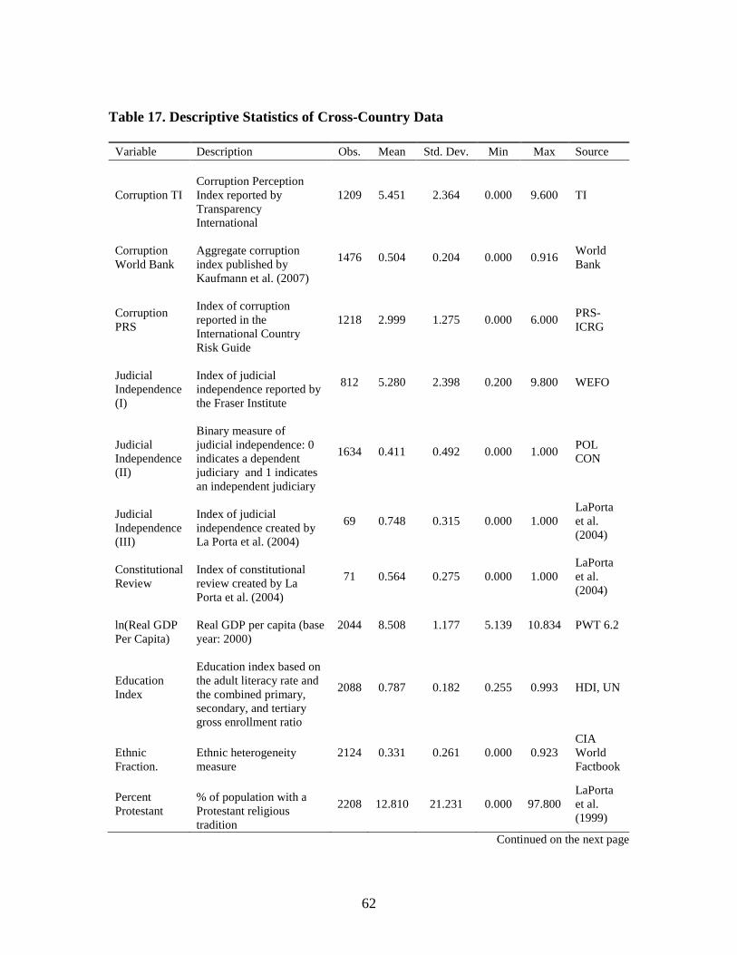
62
Table 17. Descriptive Statistics of Cross-Country Data
Variable Description Obs. Mean Std. Dev. Min Max Source
Corruption TI
Corruption Perception Index reported by Transparency International
1209 5.451 2.364 0.000 9.600 TI
Corruption World Bank
Aggregate corruption index published by Kaufmann et al. (2007)
1476 0.504 0.204 0.000 0.916 World Bank
Corruption PRS
Index of corruption reported in the International Country Risk Guide
1218 2.999 1.275 0.000 6.000 PRS-ICRG
Judicial Independence (I)
Index of judicial independence reported by the Fraser Institute
812 5.280 2.398 0.200 9.800 WEFO
Judicial Independence (II)
Binary measure of judicial independence: 0 indicates a dependent judiciary and 1 indicates an independent judiciary
1634 0.411 0.492 0.000 1.000 POL CON
Judicial Independence (III)
Index of judicial independence created by La Porta et al. (2004)
69 0.748 0.315 0.000 1.000 LaPorta et al. (2004)
Constitutional Review
Index of constitutional review created by La Porta et al. (2004)
71 0.564 0.275 0.000 1.000 LaPorta et al. (2004)
ln(Real GDP Per Capita)
Real GDP per capita (base year: 2000)
2044 8.508 1.177 5.139 10.834 PWT 6.2
Education Index
Education index based on the adult literacy rate and the combined primary, secondary, and tertiary gross enrollment ratio
2088 0.787 0.182 0.255 0.993 HDI, UN
Ethnic Fraction.
Ethnic heterogeneity measure
2124 0.331 0.261 0.000 0.923 CIA World Factbook
Percent Protestant
% of population with a Protestant religious tradition
2208 12.810 21.231 0.000 97.800 LaPorta et al. (1999)
Continued on the next page

63
Table 17. (continued) Variable Description Obs. Mean Std. Dev. Min Max Source
ln(Government Size)
General government spending as percentage of total consumption
2044 3.039 0.474 0.727 4.364 PWT 6.2
Common Law
Dummy = 1 for countries with a common law legal systems as opposed to civil law legal systems
1176 0.326 0.469 0.000 1.000 LaPorta et al. (1999)
Developing Country
Dummy = 1 for developing countries as reported by the World Bank Global Development Network Growth Database
2256 0.787 0.409 0.000 1.000 World Bank
ln(Investment)
Investment share of GDP
2040 2.454 0.640 0.000 3.991 PWT 6.2
Freedom of the Press Index
Freedom of the Press Index reported by the Freedom House
2184 46.570 24.694 0.000 100.000 Freedom House
Federal
Dummy = 1 for countries with a federal structure
1176 0.173 0.378 0.000 1.000 Treisman (2000)
Democratic
Dummy = 1 if the country has a democratic regime
540 0.259 0.439 0.000 1.000 Treisman (2000)
TI: Transparency International PRS-ICRG: Political Risk Services-International Country Risk Guide, Table 3B: Political Risk Components, 2006 Fraser Institute: Gwartney, J., R. Lawson, and W. Easterly: Economic Freedom of the World, 2007 Annual Report WEFO: World Economic Forum Organization POLCON: Political Constraint Index Dataset HDI, UN: Human Development Indicators, United Nations PWT 6.2: Heston, Allan, Robert Summers and Bettina Aten, Penn World Table 6.2, Center for International Comparisons of Production, Income and Prices at the university of Pennsylvania, September 2006.
64
5.3. Results
The main focus of the econometric specifications is on the existence of significant
relations between corruption and judicial independence or constitutional review. Along
with the Corruption TI index, Transparency International reports the standard deviations
of the corruption ratings: the greater the standard deviation, the greater the differences of
perceptions of a country among the sources. In my analysis, I estimate Weighted Least
Squares (WLS) regressions, with the weights being the reciprocals of the standard
deviations of the Corruption TI index.23As Treisman (2000) points out, this weighting
places an emphasis on those scores where the respondents in the surveys gave more
similar ratings than on those where the ratings were more divergent. In addition, the
Corruption World Bank index of each country is measured with different conditional
variances, reported by Kaufamn et al. (2007). Once again, to correct for
heteroskedasticity, I estimate Weighted Least Squares (WLS) regressions. The weights
are the reciprocals of the standard deviations of the Corruption World Bank index. To
check the robustness of my results, I also fit the data using OLS with White
heteroskedasticity-corrected standard errors.
Tables 18a through 18c present the results of year by year regressions of the
judicial independence measures (I), (II), and (III) on corruption TI, respectively, and
Table 18d shows the effect of constitutional review on corruption TI. To check the
sensitivity of my results to the way the variables of interest are measured, in Tables 19a,
19b, 20a, and 20b, I report the results of cross-sections regressions of judicial
23 Transparency International does not report the standard errors of the Corruption TI index for the years 2004, 2005, and 2006.

65
independence measures (I) and (II) on the other two corruption indicators, corruption
World Bank and corruption PRS, respectively. In presenting the results, I always consider
three distinct specifications. The first equation contains only the main variables, the
second specifications adds four control variables, (1) ln(GDP per capita), (2) education
index, (3) ethnic fractionalization, and (4) percent protestant, and the third specification
includes further controls, (5) ln(government size), (6) developing country, and (7)
common law.
In presenting the results, I do not include the coefficients on the control variables.
The results with respect to controls vary among regressions. However, I generally find
that corruption is lower in richer countries and in countries that have a higher percent of
population that is of Protestant religion tradition. Moreover, consistent with my
hypotheses, I find that corruption is lower in countries with common law legal systems
and is higher in developing countries. Surprisingly, the coefficient on the education index
variable and the one on the ethnic fractionalization variable are significant and have the
correct sign only in about 60% of the regressions, while the coefficient on the variable
measuring the government size is insignificant in most regressions.
Next, consider the estimation results for the judicial independence indicators. The
empirical results are consistent with my hypothesis that countries that have a relatively
more independent judiciary experience lower corruption levels, ceteris paribus. Table 18a
shows the results of year by year regressions of judicial independence (I) on corruption
TI. I report the results of WLS and OLS regressions for the years 1995 and 2000 to 2003,
and the results of OLS regressions for 2004 and 2005. The number of observations
66
increases considerably over time, from 40 observations in 1995 to 112 observations in
2005. With no controls, the estimated coefficients are all significant at the 1% level of
significance, suggesting that, on average, judicial independence is associated with lower
corruption scores. For example, for the year 2002, an increase of one point in the judicial
independence index (e.g., from Ghana, with a score of 5.2, to Greece, with a score of 6.2)
reduces corruption by 0.9 points (approximately to Hungary or Cost Rica levels), ceteris
paribus. When I add the first set of control variables to these regressions, the coefficient
estimates decrease in magnitude by approximately 40% but they remain statistically
different from zero at the 1% significance level. Adding the second set of control
variables further shrinks the parameter estimates and also reduces the number of
observations available for each year, but the coefficients remain statistically significant at
the 1% level.
Table 18b shows the results of WLS and OLS cross-section regressions of judicial
independence (II) on corruption TI for the years 1998 to 2004. Once again the estimated
parameters are statistically significant at the 1% significance level. For example, without
controls, for the year 2002, an independent judiciary reduces corruption by 4.2 points, on
average. Adding the controls in Panel B does not change the significance of my results,
but decreases the coefficients on the judicial independence variable. Again, for the year
2002, countries with an independent judiciary (the United States) have, on average, a
corruption score that is 1.18 points lower than countries with a dependent or influenced
judiciary (Albania). These results are, in general, robust to the inclusion of more controls
in Panel C. The coefficients on the judicial independence variable have the expected sign

67
and are significant at the 1% level for the years 2002 to 2004. For the years 1998, 2000,
and 2001, the parameter estimates have the correct sign, but are not statistically
significant, and for 1999 the coefficient has the predicted sign and is significant at the 5%
level.
Table 18c and 18d report the effect of judicial independence (III) and of
constitutional review on corruption. As discussed in section 5.2., these measures come
from La Porta et al. (2004). Data are only available for one year, 1995, which restricts the
number of observations to 37, especially given that 1995 was the first year when the
corruption TI was released. Nonetheless, the findings regarding judicial independence
support my hypothesis. In Table 18c, the coefficient estimates are significant at the 1%
level regardless of the specification used and suggest that an increase in judicial
independence from zero (China) to one (the United States) reduces the corruption index
by 2.52 (roughly to Spain) (Panel B).

68
Table 18a. Effect of Judicial Independence (I) on Corruption TI Dependent Variable
Corruption TI 1995 2000 2001 2002 2003 2004 2005
WLS[1] OLS[2] WLS[1] OLS[2] WLS[1] OLS[2] WLS[1] OLS[2] WLS[1] OLS[2] OLS[1] OLS[1]
A. No Controls JI (I) -1.178*** -0.917*** -0.906*** -0.901*** -0.783*** -0.799*** -0.981*** -0.821*** -1.145*** -0.861*** -0.836*** -0.824***
(-35.80) (-15.28) (-22.90) (-11.45) (-30.25) (-14.83) (-54.15) (-14.66) (-63.70) (-16.47) (-16.00) (-15.85)
Cons. 11.524*** 10.711*** 10.10*** 10.15*** 8.937*** 9.147*** 9.771*** 9.401*** 10.53 9.747*** 9.371*** 9.517***
(42.75) (21.02) (38.44) (19.52) (54.47) (30.09) (89.45) (33.82) (94.45) (37.02) (42.22) (42.08)
Obs. 40 40 61 61 77 77 91 91 100 100 108 118
R2 - 0.72 - 0.68 - 0.68 - 0.68 - 0.72 0.69 0.69
B. With Controls - 1 JI (I) -0.637*** -0.616*** -0.464*** -0.465*** -0.362*** -0.344*** -0.403*** -0.389*** -0.597*** -0.458*** -0.442*** -0.410***
(-8.25) (-4.91) (-7.26) (-6.11) (-9.20) (-6.57) (-11.64) (-8.27) (-15.62) (-8.95) (-8.78) (-7.09)
Cons. 22.646*** 22.167*** 18.03*** 19.90*** 22.34*** 21.16*** 23.12*** 18.92*** 23.63*** 18.22*** 17.30*** 16.49***
(9.76) (8.93) (18.87) (10.7) (21.49) (13.51) (36.79) (20.62) (35.82) (19.49) (19.20) (17.20)
Obs. 39 39 60 60 75 75 89 89 97 97 105 112
R2 - 0.82 - 0.86 - 0.87 - 0.87 - 0.87 0.85 0.84
C. With Controls - 2 JI (I) -0.276** -0.572** -0.306*** -0.357*** -0.259*** -0.288*** -0.262*** -0.287*** -0.216*** -0.351*** -0.394*** -0.353***
(-2.32) (-2.51) (-3.85) (-3.17) (-4.91) (-4.26) (-6.12) (-5.08) (-4.30) (-5.40) (-5.92) (-5.73)
Cons. 16.968*** 20.968*** 10.90*** 13.87 17.95*** 16.91*** 13.90*** 14.67*** 16.54*** 14.02*** 13.49*** 12.50***
(4.42) (3.63) (5.53) (5.36) (10.01) (7.28) (10.25) (9.29) (12.20) (10.02) (8.97) (8.23)
Obs. 39 39 60 60 73 73 86 86 87 87 88 87
R2 - 0.84 - 0.88 - 0.89 - 0.9 - 0.91 0.89 0.89
Notes: The table presents the results of WLS and OLS regressions. The WLS regressions use as weights the reciprocals of the standard deviations of the Corruption TI index (not available for 2004 and 2005). The OLS regressions results are based on robust standard errors. In panel A the independent variable is judicial independence (I). In panel B the independent variables are (1) judicial independence (I), (2) ln(GDP per capita), (3) education index, (4) ethnic fractionalization, and (5) percent protestant. In panel C the independent variables are (1) judicial independence (I), (2) ln(GDP per capita), (3) education index, (4) ethnic fractionalization, (5) percent protestant, (6) ln(government size), (7) developing country, and (8) common law. All variables are defined in Table 17. The numbers in parenthesis are the estimated z-statistics and t-statistics, respectively. {***,**,*} indicates significant at 1, 5 and 10 percent level, respectively.

69
Table 18b. Effect of Judicial Independence (II) on Corruption TI
Dependent Variable Corruption TI
1998 1999 2000 2001 2002 2003 2004 WLS[1] OLS[2] WLS[1] OLS[2] WLS[1] OLS[2] WLS[1] OLS[2] WLS[1] OLS[2] WLS[1] OLS[2] OLS[1]
A. No Controls JI (II) -3.182*** -2.408*** -3.480*** -2.630*** -2.836*** -2.624*** -3.274*** -2.647*** -4.218*** -2.790*** -4.570*** -2.706*** -2.741***
(-18.25) (-6.32) (-23.53) (-7.22) (-20.85) (-6.98) (-25.99) (-7.06) (-44.27) (-7.80) (-58.28) (-7.47) (-8.19)
Cons. 6.953*** 6.837*** 7.237*** 6.944*** 7.178*** 6.875*** 7.009** 6.920*** 7.415*** 6.997*** 6.710*** 6.937*** 7.041***
(49.17) (33.29) (70.42) (39.13) (73.07) (36.50) (71.69) (35.36) (100.68) (46.95) (129.94) (50.12) (57.21)
Obs. 83 83 95 95 88 88 90 90 101 101 129 129 138
R2 - 0.20 - 0.30 - 0.28 - 0.29 - 0.35 - 0.34 0.36
B. With Controls - 1
JI (II) -0.890*** -0.738** -1.259*** -0.881*** -0.861*** -0.762*** -0.779*** -0.708*** -1.186*** -0.937*** -2.587*** -0.981*** -1.119***
(-4.09) (-2.62) (-6.49) (-3.66) (-4.83) (-3.28) (-4.94) (-2.99) (-9.90) (-4.19) (-25.57) (-4.39) (-5.14)
Cons. 21.106*** 19.882*** 19.381*** 18.841*** 18.798*** 19.575*** 22.242*** 20.822*** 25.241*** 20.101*** 20.221*** 18.430*** 17.214***
(24.68) (13.39) (25.72) (14.86) (29.63) (16.73) (33.36) (17.19) (47.48) (17.87) (56.68) (19.68) (18.73)
Obs. 82 82 93 93 85 85 88 88 99 99 121 121 129
R2 - 0.77 - 0.79 - 0.82 - 0.83 - 0.83 - 0.78 0.76
C. With Controls - 2
JI (II) -0.322 -0.218 -0.604** -0.466* -0.143 -0.312 -0.192 -0.286 -0.594*** -0.463* -0.748*** -0.607** -0.748***
(-1.40) (-0.83) (-2.54) (-1.91) (-0.59) (-1.21) (-1.02) (-0.99) (-3.79) (-1.88) (-4.13) (-2.49) (-2.90)
Cons. 13.972*** 14.200*** 13.280*** 14.170*** 13.251*** 14.625*** 17.749*** 16.706*** 15.700*** 16.104*** 16.992*** 14.889*** 13.653***
(9.71) (8.33) (8.51) (8.02) (8.40) (7.52) (12.01) (9.48) (12.45) (10.56) (12.87) (10.47) (9.37)
Obs. 81 81 82 82 75 75 82 82 89 89 92 92 93
R2 - 0.85 - 0.86 - 0.87 - 0.87 - 0.88 - 0.88 -
Notes: The table presents the results of WLS and OLS regressions. The WLS regressions use as weights the reciprocals of the standard deviations of the Corruption TI index (not available for 2004). The OLS regressions results are based on robust standard errors. In panel A the independent variable is judicial independence (II), i.e., JI (II). In panel B the independent variables are (1) JI (II), (2) ln(GDP per capita), (3) education index, (4) ethnic fractionalization, and (5) percent protestant. In panel C the independent variables are (1) JI (II), (2) ln(GDP per capita), (3) education index, (4) ethnic fractionalization, (5) percent protestant, (6) ln(government size), (7) developing country, and (8) common law. All variables are defined in Table 17. The numbers in parenthesis are the estimated z and t-statistics, respectively. {***,**,*} indicates significant at 1, 5 and 10 percent level, respectively.
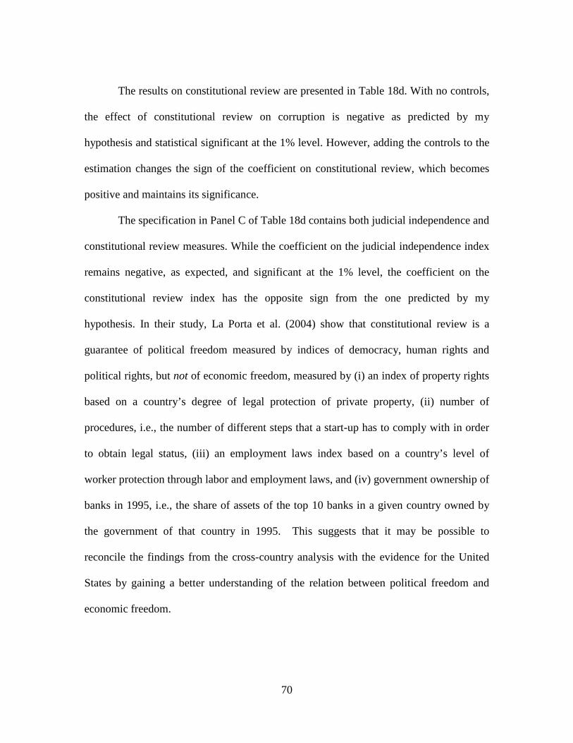
70
The results on constitutional review are presented in Table 18d. With no controls,
the effect of constitutional review on corruption is negative as predicted by my
hypothesis and statistical significant at the 1% level. However, adding the controls to the
estimation changes the sign of the coefficient on constitutional review, which becomes
positive and maintains its significance.
The specification in Panel C of Table 18d contains both judicial independence and
constitutional review measures. While the coefficient on the judicial independence index
remains negative, as expected, and significant at the 1% level, the coefficient on the
constitutional review index has the opposite sign from the one predicted by my
hypothesis. In their study, La Porta et al. (2004) show that constitutional review is a
guarantee of political freedom measured by indices of democracy, human rights and
political rights, but not of economic freedom, measured by (i) an index of property rights
based on a country’s degree of legal protection of private property, (ii) number of
procedures, i.e., the number of different steps that a start-up has to comply with in order
to obtain legal status, (iii) an employment laws index based on a country’s level of
worker protection through labor and employment laws, and (iv) government ownership of
banks in 1995, i.e., the share of assets of the top 10 banks in a given country owned by
the government of that country in 1995. This suggests that it may be possible to
reconcile the findings from the cross-country analysis with the evidence for the United
States by gaining a better understanding of the relation between political freedom and
economic freedom.

71
Table 18c. Effect of Judicial Independence (III) on Corruption TI
Dependent Variable Corruption TI
WLS[1] OLS[2] Coeff. Coeff.
(z) (t) A. No Controls
Judicial Independence (III) -7.307*** -4.041***
(-31.38) (-3.25)
Constant 8.471*** 7.303***
(39.92) (7.86)
Observations 38 38
R2 - 0.16
B. With Controls - 1 Judicial Independence (III) -2.524*** -2.027*
(-4.46) (-1.87)
Constant 28.064*** 27.157***
(11.34) (7.23)
Observations 37 37
R2 - 0.76
C. With Controls – 2 Judicial Independence (III) -1.681*** -2.037***
(-2.79) (-2.04)
Constant 12.809** 24.818***
(2.51) (3.15)
Observations 37 37
R2 - 0.77
Notes: The table presents the results of WLS and OLS regressions. The WLS regressions use as weights the reciprocals of the standard deviations of the Corruption TI index. The OLS regressions results are based on robust standard errors. In panel A the independent variable is judicial independence (III). In panel B the independent variables are (1) judicial independence (III), (2) ln(GDP per capita), (3) education index, (4) ethnic fractionalization, and (5) percent protestant. In panel C the independent variables are (1) judicial independence (III), (2) ln(GDP per capita), (3) education index, (4) ethnic fractionalization, (5) percent protestant, (6) ln(government size), and (7) developing country. All variables are defined in Table 17. The numbers in parenthesis are the estimated z-statistics and t-statistics, respectively. {***,**,*} indicates significant at 1, 5 and 10 percent level, respectively.
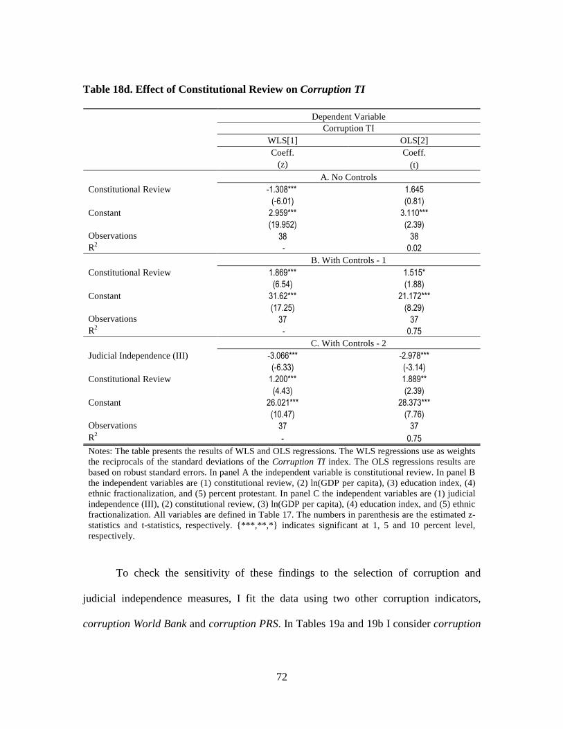
72
Table 18d. Effect of Constitutional Review on Corruption TI
Dependent Variable Corruption TI
WLS[1] OLS[2] Coeff. Coeff.
(z) (t) A. No Controls
Constitutional Review -1.308*** 1.645
(-6.01) (0.81)
Constant 2.959*** 3.110***
(19.952) (2.39)
Observations 38 38
R2 - 0.02
B. With Controls - 1 Constitutional Review 1.869*** 1.515*
(6.54) (1.88)
Constant 31.62*** 21.172***
(17.25) (8.29)
Observations 37 37
R2 - 0.75
C. With Controls - 2 Judicial Independence (III) -3.066*** -2.978***
(-6.33) (-3.14)
Constitutional Review 1.200*** 1.889**
(4.43) (2.39)
Constant 26.021*** 28.373***
(10.47) (7.76)
Observations 37 37
R2 - 0.75
Notes: The table presents the results of WLS and OLS regressions. The WLS regressions use as weights the reciprocals of the standard deviations of the Corruption TI index. The OLS regressions results are based on robust standard errors. In panel A the independent variable is constitutional review. In panel B the independent variables are (1) constitutional review, (2) ln(GDP per capita), (3) education index, (4) ethnic fractionalization, and (5) percent protestant. In panel C the independent variables are (1) judicial independence (III), (2) constitutional review, (3) ln(GDP per capita), (4) education index, and (5) ethnic fractionalization. All variables are defined in Table 17. The numbers in parenthesis are the estimated z-statistics and t-statistics, respectively. {***,**,*} indicates significant at 1, 5 and 10 percent level, respectively.
To check the sensitivity of these findings to the selection of corruption and
judicial independence measures, I fit the data using two other corruption indicators,
corruption World Bank and corruption PRS. In Tables 19a and 19b I consider corruption

73
World Bank as my measure of corruption. Table 19a shows the results of WLS and OLS
cross-section regressions for the years 2000 to 2005. The number of observations varies
from 61 in 2000 to 119 in 2005. Once more, the effect of the judicial independence (I)
measure is significant at the 1% level and has the predicted sign. Without controls, for
example, for the year 2002, the estimates suggest that, everything else constant, an
increase in judicial independence of one point reduces the corruption index by 0.075
units. The regressions in panels B and C introduce the same control variables used in the
specifications reported in Tables 18a-b. The results are similar with those from the
previous findings. Even though the estimates get smaller once I introduce additional
controls, they all remain significant at the 1% level and have the predicted sign in all the
regressions. Moreover, the parameter estimates do not change considerably depending on
the estimation technique, but the z-statistics are smaller in the WLS regressions.
Table 19b shows the effect of the judicial independence (II) measure on
corruption World Bank. The estimates without controls are all significant at the 1% level
and have the expected signs. Except for the year 2000, for which the coefficient on
judicial independence is not statistically significant, adding the controls in Panel B does
not affect the significance or the sign of the estimates. The second set of controls has a
different impact on the results. The 1998 and 2000 coefficient estimates become
statistically insignificant, while the significance of the 2000 estimates decreases to the
10% level. The 2003 and 2004 estimates are statistically significant at the 1% level.
The results with regard to the corruption PRS indicator are presented in Tables
20a and b. Once again the estimates are consistent with my previous findings.

Table 19a. The Effect of Judicial Independence (I) on Corruption World Bank
Dependent Variable Corruption World Bank
2000 2002 2003 2004 2005 WLS[1] OLS[2] WLS[1] OLS[2] WLS[1] OLS[2] WLS[1] OLS[2] WLS[1] OLS[2]
A. No Controls JI (I) -0.080*** -0.079*** -0.075*** -0.075*** -0.076*** -0.077*** -0.075*** -0.075*** -0.073*** -0.074***
(-8.68) (-14.04) (-10.76) (-15.74) (-11.50) (-18.50) (-12.01) (-16.51) (-12.47) (-17.55)
Cons. 0.870*** 0.855*** 0.825*** 0.823*** 0.827*** 0.834*** 0.808*** 0.807*** 0.825*** 0.833***
(14.58) (22.15) (21.16) (35.06) (22.56) (37.29) (24.26) (39.73) -25.95 (42.62)
Obs. 63 63 96 96 102 102 109 109 119 119
R2 - 0.64 - 0.65 - 0.72 - 0.67 - 0.70
B. With Controls - 1 JI (I) -0.042*** -0.038*** -0.036*** -0.036*** -0.040*** -0.041*** -0.037*** -0.037*** -0.037*** -0.038***
(-2.96) (-6.48) (-3.53) (-7.34) (-3.94) (-8.55) (-4.11) (-8.14) (-4.10) (-7.71)
Cons. 1.981*** 1.982*** 1.822*** 1.742*** 1.667*** 1.601*** 1.706*** 1.624*** 1.562*** 1.479***
(7.09) (13.64) (9.35) (12.90) (9.76) (15.55) (11.08) (16.99) (10.15) (15.64)
Obs. 62 62 94 94 99 99 105 105 113 113
R2 - 0.89 - 0.85 - 0.87 - 0.86 - 0.85
C. With Controls - 2 JI (I) -0.036*** -0.031*** -0.032*** -0.033*** -0.036*** -0.036*** -0.035*** -0.035*** -0.033*** -0.034***
(-1.95) (-4.39) (-2.64) (-6.16) (-2.87) (-6.69) (-2.95) (-6.28) (-2.89) (-6.83)
Cons. 1.578*** 1.627*** 1.391*** 1.379*** 1.330*** 1.325*** 1.377*** 1.370*** 1.405*** 1.398***
(3.16) (7.07) (3.96) (9.63) (4.27) (10.96) (4.54) (11.23) (4.71) (11.26)
Obs. 61 61 87 87 87 87 88 88 87 87
R2 - 0.9 - 0.91 - 0.91 - 0.90 - 0.91
Notes: The table presents the results of WLS and OLS regressions. The WLS regressions use as weights the reciprocals of the standard deviations of the Corruption World Bank index. The OLS regressions results are based on robust standard errors. In panel A the independent variable is judicial independence (I). In panel B the independent variables are (1) judicial independence (I), (2) ln(GDP per capita), (3) education index, (4) ethnic fractionalization, and (5) percent protestant. In panel C the independent variables are (1) judicial independence (I), (2) ln(GDP per capita), (3) education index, (4) ethnic fractionalization, (5) percent protestant, (6) ln(government size), (7) developing country, and (8) common law. All variables are defined in Table 17. The numbers in parenthesis are the estimated z-statistics and t-statistics, respectively. {***,**,*} indicates significant at 1, 5, and 10 percent level, respectively.
74
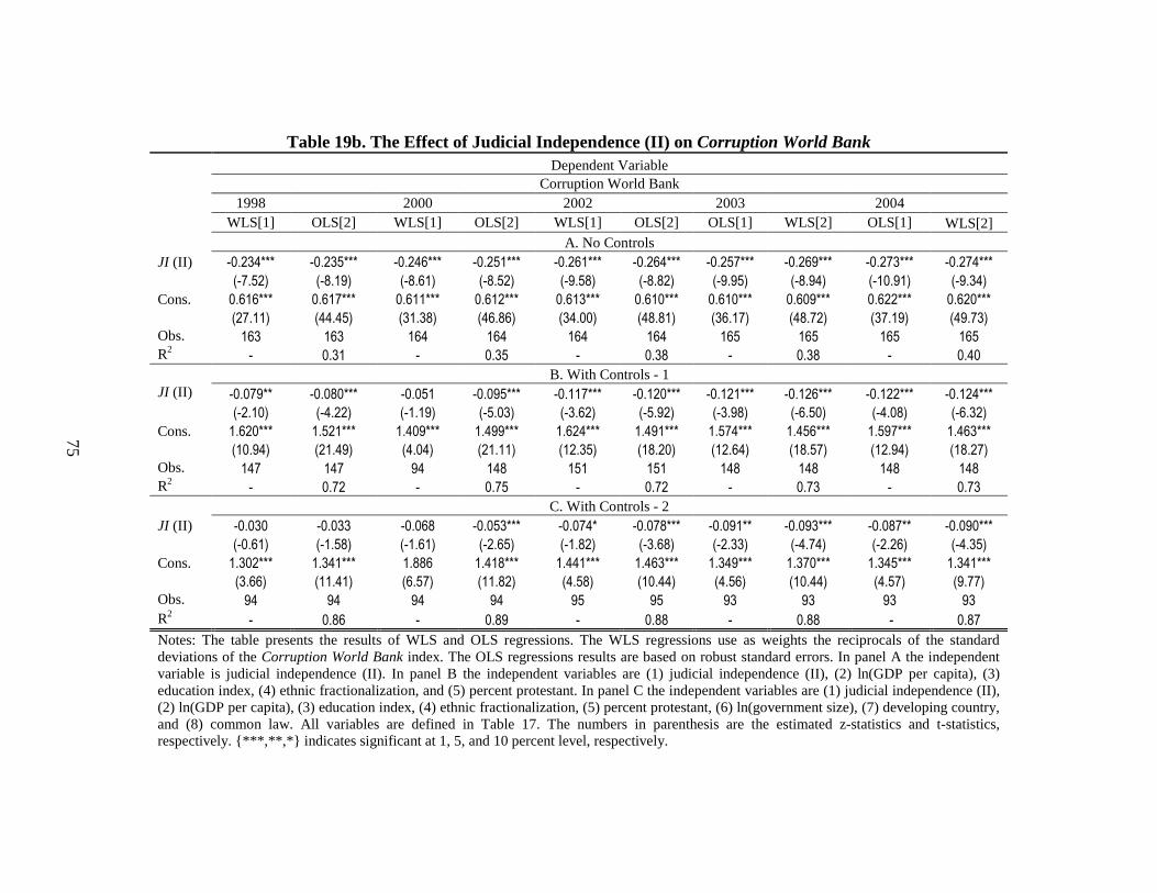
Table 19b. The Effect of Judicial Independence (II) on Corruption World Bank Dependent Variable
Corruption World Bank 1998 2000 2002 2003 2004
WLS[1] OLS[2] WLS[1] OLS[2] WLS[1] OLS[2] OLS[1] WLS[2] OLS[1] WLS[2] A. No Controls
JI (II) -0.234*** -0.235*** -0.246*** -0.251*** -0.261*** -0.264*** -0.257*** -0.269*** -0.273*** -0.274***
(-7.52) (-8.19) (-8.61) (-8.52) (-9.58) (-8.82) (-9.95) (-8.94) (-10.91) (-9.34)
Cons. 0.616*** 0.617*** 0.611*** 0.612*** 0.613*** 0.610*** 0.610*** 0.609*** 0.622*** 0.620***
(27.11) (44.45) (31.38) (46.86) (34.00) (48.81) (36.17) (48.72) (37.19) (49.73)
Obs. 163 163 164 164 164 164 165 165 165 165
R2 - 0.31 - 0.35 - 0.38 - 0.38 - 0.40
B. With Controls - 1 JI (II) -0.079** -0.080*** -0.051 -0.095*** -0.117*** -0.120*** -0.121*** -0.126*** -0.122*** -0.124***
(-2.10) (-4.22) (-1.19) (-5.03) (-3.62) (-5.92) (-3.98) (-6.50) (-4.08) (-6.32)
Cons. 1.620*** 1.521*** 1.409*** 1.499*** 1.624*** 1.491*** 1.574*** 1.456*** 1.597*** 1.463***
(10.94) (21.49) (4.04) (21.11) (12.35) (18.20) (12.64) (18.57) (12.94) (18.27)
Obs. 147 147 94 148 151 151 148 148 148 148
R2 - 0.72 - 0.75 - 0.72 - 0.73 - 0.73
C. With Controls - 2 JI (II) -0.030 -0.033 -0.068 -0.053*** -0.074* -0.078*** -0.091** -0.093*** -0.087** -0.090***
(-0.61) (-1.58) (-1.61) (-2.65) (-1.82) (-3.68) (-2.33) (-4.74) (-2.26) (-4.35)
Cons. 1.302*** 1.341*** 1.886 1.418*** 1.441*** 1.463*** 1.349*** 1.370*** 1.345*** 1.341***
(3.66) (11.41) (6.57) (11.82) (4.58) (10.44) (4.56) (10.44) (4.57) (9.77)
Obs. 94 94 94 94 95 95 93 93 93 93
R2 - 0.86 - 0.89 - 0.88 - 0.88 - 0.87
Notes: The table presents the results of WLS and OLS regressions. The WLS regressions use as weights the reciprocals of the standard deviations of the Corruption World Bank index. The OLS regressions results are based on robust standard errors. In panel A the independent variable is judicial independence (II). In panel B the independent variables are (1) judicial independence (II), (2) ln(GDP per capita), (3) education index, (4) ethnic fractionalization, and (5) percent protestant. In panel C the independent variables are (1) judicial independence (II), (2) ln(GDP per capita), (3) education index, (4) ethnic fractionalization, (5) percent protestant, (6) ln(government size), (7) developing country, and (8) common law. All variables are defined in Table 17. The numbers in parenthesis are the estimated z-statistics and t-statistics, respectively. {***,**,*} indicates significant at 1, 5, and 10 percent level, respectively.
75

Table 20a. The Effect of Judicial Independence (I) on Corruption PRS Dependent Variable
Corruption PRS 2000 2001 2002 2003 Coeff. Coeff. Coeff. Coeff.
(t) (t) (t) (t) A. No Controls
Judicial Independence (I) -0.358*** -0.319*** -0.377*** -0.369***
(-5.95) (-6.60) (-9.35) (-9.24)
Constant 4.700*** 4.443*** 5.189*** 5.151***
(12.61) (16.08) (25.23) (23.89)
Observations 61 82 94 98
R2 0.37 0.38 0.53 0.50
B. With Controls - 1 Judicial Independence (I) -0.158** -0.072 -0.190*** -0.215***
(-2.22) (-1.15) (-4.46) (-4.28)
Constant 8.751*** 10.804*** 8.687*** 7.648***
(6.19) (8.58) (7.96) (7.18)
Observations 60 80 92 95
R2 0.56 0.57 0.65 0.57
C. With Controls - 2 Judicial Independence (I) -0.163* -0.123* -0.157*** -0.177***
(-1.83) (-1.73) (-3.06) (-3.26)
Constant 8.032*** 9.628*** 6.336*** 5.078***
(2.87) (5.24) (4.95) (4.15)
Observations 59 77 86 86
R2 0.58 0.64 0.77 0.75
Notes: The table presents the results of OLS regressions based on robust standard errors. In panel A the independent variable is judicial independence (I). In panel B the independent variables are (1) judicial independence (I), (2) ln(GDP per capita), (3) education index, (4) ethnic fractionalization, and (5) percent protestant. In panel C the independent variables are (1) judicial independence (I), (2) ln(GDP per capita), (3) education index, (4) ethnic fractionalization, (5) percent protestant, (6) ln(government size), (7) developing country, and (8) common law. All variables are defined in Table 17. The numbers in parenthesis are the estimated t-statistics. {***,**,*} indicates significant at 1, 5 and 10 percent level, respectively.
76
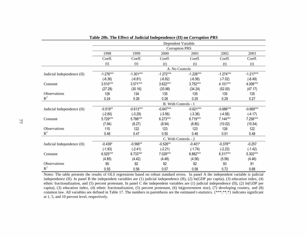
Table 20b. The Effect of Judicial Independence (II) on Corruption PRS Dependent Variable
Corruption PRS 1998 1999 2000 2001 2002 2003 Coeff. Coeff. Coeff. Coeff. Coeff. Coeff.
(t) (t) (t) (t) (t) (t) A. No Controls
Judicial Independence (II) -1.276*** -1.301*** -1.272*** -1.226*** -1.274*** -1.217***
(-6.36) (-6.81) (-6.82) (-6.56) (-7.02) (-6.49)
Constant 3.510*** 3.571*** 3.622*** 3.752*** 4.101*** 4.006***
(27.28) (30.16) (33.98) (34.24) (52.00) (47.17)
Observations 126 134 135 135 135 135
R2 0.24 0.26 0.26 0.25 0.29 0.27
B. With Controls - 1 Judicial Independence (II) -0.519** -0.613*** -0.647*** -0.621*** -0.686*** -0.669***
(-2.60) (-3.29) (-3.56) (-3.36) (-4.56) (-4.17)
Constant 5.729*** 5.788*** 6.273*** 6.719*** 7.144*** 7.256***
(7.94) (8.27) (8.94) (8.80) (10.02) (10.54)
Observations 115 122 123 123 126 122
R2 0.46 0.47 0.50 0.46 0.51 0.48
C. With Controls - 2 Judicial Independence (II) -0.439* -0.566** -0.526** -0.401* -0.378** -0.257
(-1.93) (-2.41) (-2.21) (-1.74) (-2.23) (-1.42)
Constant 6.525*** 6.733*** 7.029*** 6.882*** 6.317*** 5.302***
(4.85) (4.42) (4.48) (4.56) (5.56) (4.46)
Observations 90 92 92 92 93 91
R2 0.55 0.56 0.57 0.58 0.72 0.68
Notes: The table presents the results of OLS regressions based on robust standard errors. In panel A the independent variable is judicial independence (II). In panel B the independent variables are (1) judicial independence (II), (2) ln(GDP per capita), (3) education index, (4) ethnic fractionalization, and (5) percent protestant. In panel C the independent variables are (1) judicial independence (II), (2) ln(GDP per capita), (3) education index, (4) ethnic fractionalization, (5) percent protestant, (6) ln(government size), (7) developing country, and (8) common law. All variables are defined in Table 17. The numbers in parenthesis are the estimated t-statistics. {***,**,*} indicates significant at 1, 5, and 10 percent level, respectively.
77

84
In Table 20a, I present the result of OLS cross-sections regressions for the years
2000 to 2003. With controls, the coefficient estimates are significant at the 1% percent
level and have the predicted sign. When I add the first set of controls, some of the
coefficients on the judicial independence variable maintain their signs but become less
significant: for the year 2000, the coefficient is significant at the 5% level, for 2001, the
coefficient is insignificant, and for 2002 – 2003, the coefficients remain significant at the
1% level. Adding the second set of controls does not change much the significance of my
results: the years 2000-2001 are still significant at the 10% level, while 2002-2003 are
significant at the 1% level. For the year 2002 for example, the estimates suggest that an
increase in judicial independence of one point (from Malawi, with a score of six, to
Ireland, with a score of seven) reduces the corruption index by 0.15 (roughly to the
United States level), on average. Table 20b shows the results on judicial independence
(II). Without controls and with the first set of controls, the coefficient estimates have the
expected sign and are significant at the 1% level. When I add the second set of controls,
the coefficients became slightly smaller in magnitude and significant at the 5% level
(years 1999, 2000, and 2002) or 10% level (years 1998 and 2001).
Overall, it appears that the relation between judicial independence and corruption
is robust to the way corruption and judicial independence levels are measured, to the
estimation technique, and in general to the inclusion of various control variables.
78

79
5.4. Additional Robustness Checks
This section extends my analysis of the effect of judicial independence on
corruption to panels of data with cross-sectional and time-series observations for 1998 to
2005. Tables 21 through 23 report the results of pooled OLS, WLS, and panel data
regressions using corruption TI, corruption World Bank, and corruption PRS,
respectively, as dependent variables, and judicial independence (I), (II), and controls as
independent variables. One of the key issues when considering panel data regressions is
the choice of estimator. I believe that the "between" estimator would best fit my models,
since this estimator captures the cross-country information in the data. Moreover, my
variables of interest, as well as many of the controls, exhibit very little variation over
time. Therefore, the information content of the data corresponds to a great extent to the
cross-country variation in the data.
For completeness I also report the results of “random effects” and “fixed effects”
estimations. The presence of time invariant independent variables in the specification
makes it difficult to use a “fixed effects” model. To facilitate this, I decompose every
time variant variable in the model into two variables: average(s) and delta(s). Average is
just the mean of each variable over the sample period, by country, while delta is the
difference from the mean. I then fit a random effects model on all averages and deltas
along with the variables that do not vary over time. The coefficients I obtain should equal
the coefficients that would be estimated separately by the "between" estimator and the
"fixed-effects" estimator, respectively. Table 21 reports the results of panel regressions of
both judicial independence measures on Corruption TI for the years 2000-2005 and 1998-
80
2004, respectively. With or without controls, the coefficient estimates are significant at
the 1% level and have the predicted sign. In Table 22, the dependent variable is replaced
by the Corruption World Bank index. The results look similar to those presented in Table
21, except for the “fixed effects” estimator, for which the coefficient estimates are not
significant. This is no surprise since, as I mentioned above, most of the information
contained in the data comes from the cross-country variation. The results presented in
table 23 are very similar to those in table 22. The parameter estimates are significant at
the 1% level and have the sign predicted by my hypothesis, except for the “fixed effects”
estimator. These additional robustness checks provide further evidence in support of my
hypothesis that judicial independence is associated with lower corruption levels.

Table 21. Effect of Judicial Independence on Corruption TI: Pooled OLS, WLS, and Panel Estimations Dependent Variable
Corruption TI
Independent Variable Judicial Independence (I) Judicial Independence (II) 2000 - 2005 1998 - 2004
OLS[1] WLS[2] BE[3] FE[4] RE[5] OLS[1] WLS[2] BE[3]
A. With Controls - 1 Judicial Independence -0.400*** -0.452*** -0.447*** -0.053** -0.123*** -1.077*** -1.637*** -1.375***
(-18.23) (-23.03) (-8.34) (-2.57) (-6.16) (-11.58) (-24.40) (-5.37)
Constant 17.996*** 23.967*** 16.498*** 16.496*** 17.849*** 19.148*** 22.567*** 16.954***
(31.04) (54.26) (20.26) (20.68) (24.93) (36.38) (70.91) (16.01)
Observations 473 289 538 538 538 582 480 582
R2 0.87 - 0.87 0.02 0.82 0.81 - 0.81
B. With Controls - 2 Judicial Independence -0.315*** -0.249*** -0.388*** -0.063*** -0.097*** -0.587*** -0.659*** -0.753***
(-12.25) (-10.26) (-5.87) (-3.02) (-4.80) (-5.80) (-8.33) (-2.91)
Constant 14.576*** 15.172*** 13.332*** 13.403*** 13.756*** 15.752*** 14.781*** 16.304***
(17.98) (16.89) (8.27) (8.29) (10.35) (19.94) (21.34) (8.03)
Observations 445 284 481 481 481 540 457 540
R2 0.90 - 0.90 0.03 0.87 0.87 - 0.89
C. With Controls - 3 Judicial Independence -0.317*** -0.284*** -0.377*** -0.063*** -0.096*** -0.597*** -0.727*** -0.753***
(-12.58) (-11.72) (-5.56) (-2.98) (-4.65) (-5.82) (-9.06) (-2.82)
Constant 15.324*** 17.524*** 13.112*** 13.028*** 14.110*** 15.997*** 15.612*** 16.249***
(16.82) (19.23) (7.19) (6.94) (10.21) (17.20) (20.84) (6.97)
Observations 442 321 478 478 478 540 457 540
R2 0.90 - 0.90 0.05 0.87 0.87 - 0.89
Notes: The pooled OLS regressions results are based on robust standard errors. The pooled WLS regressions use as weights the standard deviations of the perceived corruption levels. Using panel data, I report the “between estimation” results, and the results of estimations with fixed effects and random effects. In panel A the independent variables are (1) judicial independence, (2) ln(GDP per capita), (3) education index, (4) ethnic fractionalization, and (5) percent protestant. In panel B the independent variables are those included in panel A plus (6) ln(government size), (7) developing country, and (8) common law. In panel C the independent variables are those included in panel B plus (9) ln(investment), (10) federal, and (11) freedom of the press index. All variables are defined in Table 17. The numbers in parenthesis are the estimated t-statistics and z-statistics, respectively. {***,**,*} indicates significant at 1, 5 and 10 percent level, respectively.
81
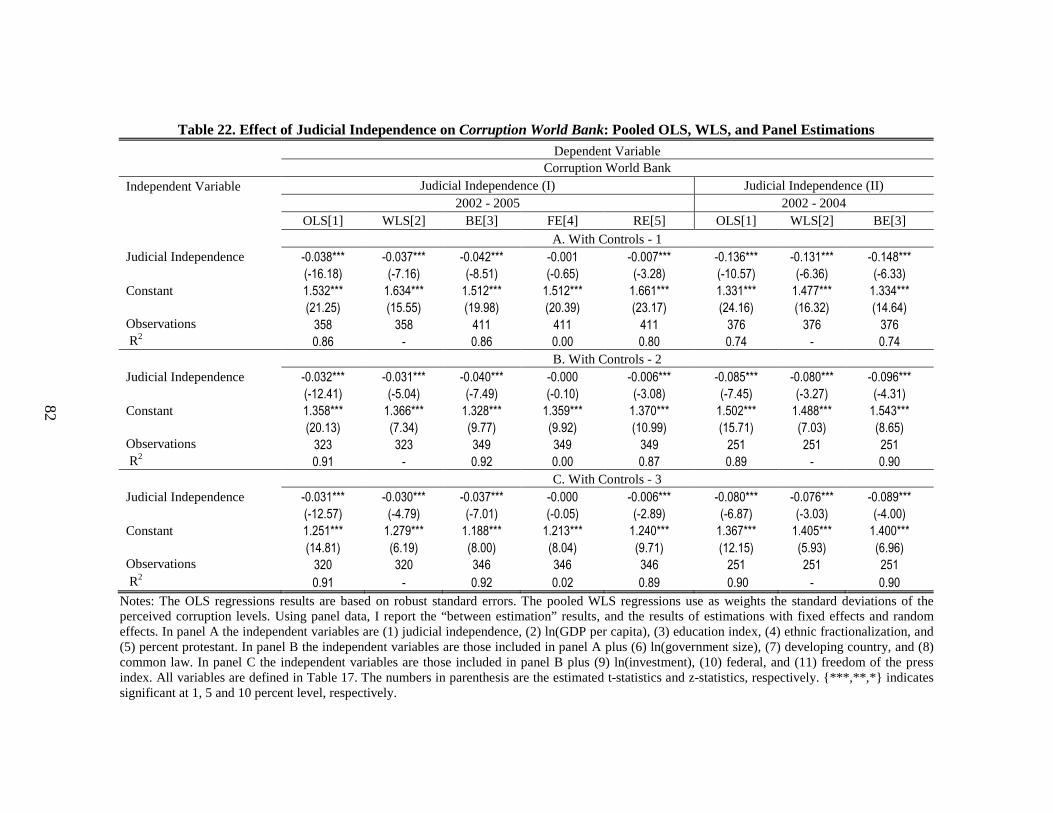
Table 22. Effect of Judicial Independence on Corruption World Bank: Pooled OLS, WLS, and Panel Estimations Dependent Variable
Corruption World Bank
Independent Variable Judicial Independence (I) Judicial Independence (II) 2002 - 2005 2002 - 2004
OLS[1] WLS[2] BE[3] FE[4] RE[5] OLS[1] WLS[2] BE[3]
A. With Controls - 1 Judicial Independence -0.038*** -0.037*** -0.042*** -0.001 -0.007*** -0.136*** -0.131*** -0.148***
(-16.18) (-7.16) (-8.51) (-0.65) (-3.28) (-10.57) (-6.36) (-6.33)
Constant 1.532*** 1.634*** 1.512*** 1.512*** 1.661*** 1.331*** 1.477*** 1.334***
(21.25) (15.55) (19.98) (20.39) (23.17) (24.16) (16.32) (14.64)
Observations 358 358 411 411 411 376 376 376
R2 0.86 - 0.86 0.00 0.80 0.74 - 0.74
B. With Controls - 2 Judicial Independence -0.032*** -0.031*** -0.040*** -0.000 -0.006*** -0.085*** -0.080*** -0.096***
(-12.41) (-5.04) (-7.49) (-0.10) (-3.08) (-7.45) (-3.27) (-4.31)
Constant 1.358*** 1.366*** 1.328*** 1.359*** 1.370*** 1.502*** 1.488*** 1.543***
(20.13) (7.34) (9.77) (9.92) (10.99) (15.71) (7.03) (8.65)
Observations 323 323 349 349 349 251 251 251
R2 0.91 - 0.92 0.00 0.87 0.89 - 0.90
C. With Controls - 3 Judicial Independence -0.031*** -0.030*** -0.037*** -0.000 -0.006*** -0.080*** -0.076*** -0.089***
(-12.57) (-4.79) (-7.01) (-0.05) (-2.89) (-6.87) (-3.03) (-4.00)
Constant 1.251*** 1.279*** 1.188*** 1.213*** 1.240*** 1.367*** 1.405*** 1.400***
(14.81) (6.19) (8.00) (8.04) (9.71) (12.15) (5.93) (6.96)
Observations 320 320 346 346 346 251 251 251
R2 0.91 - 0.92 0.02 0.89 0.90 - 0.90
Notes: The OLS regressions results are based on robust standard errors. The pooled WLS regressions use as weights the standard deviations of the perceived corruption levels. Using panel data, I report the “between estimation” results, and the results of estimations with fixed effects and random effects. In panel A the independent variables are (1) judicial independence, (2) ln(GDP per capita), (3) education index, (4) ethnic fractionalization, and (5) percent protestant. In panel B the independent variables are those included in panel A plus (6) ln(government size), (7) developing country, and (8) common law. In panel C the independent variables are those included in panel B plus (9) ln(investment), (10) federal, and (11) freedom of the press index. All variables are defined in Table 17. The numbers in parenthesis are the estimated t-statistics and z-statistics, respectively. {***,**,*} indicates significant at 1, 5 and 10 percent level, respectively.
82

Table 23. Effect of Judicial Independence on Corruption PRS: Pooled OLS and Panel Estimations Dependent Variable
Corruption PRS
Independent Variable Judicial Independence (I) Judicial Independence (II) 2000 - 2003 1998 - 2003
OLS[1] BE[3] FE[4] RE[5] OLS[1] BE[2]
A. With Controls - 1 Judicial Independence -0.179*** -0.187*** -0.066 -0.159*** -0.656*** -0.624***
(-6.09) (-3.77) (-1.41) (-4.50) (-8.12) (-3.23)
Constant 7.639*** 7.669*** 7.607*** 7.539*** 5.924*** 6.047***
(10.78) (9.52) (9.40) (9.38) (15.11) (7.64)
Observations 297 327 327 327 620 620
R2 0.61 0.62 0.11 0.57 0.49 0.57
B. With Controls - 2 Judicial Independence -0.145*** -0.180** -0.060 -0.138*** -0.487*** -0.387*
(-4.39) (-3.24) (-1.24) (-3.61) (-5.26) (-1.87)
Constant 6.033*** 6.568*** 6.249*** 5.817*** 6.024*** 6.456***
(6.77) (4.83) (4.52) (4.18) (8.67) (3.82)
Observations 286 308 308 308 492 492
R2 0.68 0.75 0.11 0.66 0.61 0.71
C. With Controls - 3 Judicial Independence -0.141*** -0.161*** -0.052 -0.127*** -0.394*** -0.259
(-4.50) (-2.90) (-1.06) (3.29) (-4.36) (-1.24)
Constant 4.824*** 5.209*** 4.516*** 4.906*** 4.577*** 4.716**
(4.66) (3.46) (2.93) (3.25) (5.77) (2.63)
Observations 284 306 306 306 492 492
R2 0.68 0.77 0.13 0.67 0.63 0.74
Notes: The OLS regressions results are based on robust standard errors. The panel regressions use the between estimation method. In panel A the independent variables are (1) judicial independence, (2) ln(GDP per capita), (3) education index, (4) ethnic fractionalization, and (5) percent protestant. In panel B the independent variables are those included in panel A plus (6) ln(government size), (7) developing country, and (8) common law. In panel C the independent variables are those included in panel B plus (9) ln(investment), (10) federal, and (11) freedom of the press index. All variables are defined in Table 17. The numbers in parenthesis are the estimated t-statistics and z-statistics, respectively. {***,**,*} indicates significant at 1, 5 and 10 percent level, respectively.
83

84
5.5. Conclusions
The development of several country-level corruption indicators in the 1990s made
it possible to study the causes and consequences of corruption, and numerous authors
have done so over the last 15 years. Previous empirical studies focused less on the legal
environment, and mainly on aspects related to the political, economic, cultural, and socio-
demographic environment of each country. This research addresses the importance of
judicial checks and balances in predicting corruption levels. Using cross-sections of data
for various years between 1995 and 2005, I investigate empirically the effect of judicial
independence and constitutional review on corruption. I find strong support in favor of
my hypothesis that higher judicial independence is associated with lower corruption
levels, ceteris paribus. To eliminate suspicions that survey-based indicators do not
accurately measure the variables of interest, I conduct the empirical analysis using three
distinct sets of corruption and judicial independence indicators. In general, the estimation
results are not sensitive to the way corruption is measured.
There is always the possibility that my analysis is affected by endogeneity, i.e.,
there may be unobserved country characteristics that affect both institutional design and
corruption outcomes. Nonetheless, it is encouraging that my results are generally
consistent with my hypotheses concerning the relation between corruption and
characteristics of the legal system. Further work and estimations with suitable
instrumental variables will be required to establish firm policy implications regarding the
effect of judicial independence or constitutional review on corruption.

85
CHAPTER SIX
CONCLUSIONS
Judicial oversight provides an important check on the abuse of power by the
legislative and executive branches. I investigate the relation between two distinct
components of the oversight function — judicial independence and constitutional rigidity
— and a specific type of abuse of power by government officials: corruption in public
office. I carry out my analysis using measures of corruption derived from criminal
convictions data and measures of corruption derived from survey data. In the case of the
former, I propose a new empirical strategy that explicitly recognizes the distinction
between the unobserved number of corrupt officials and the observed number of
convictions for corruption. I show that by including variables that pick up differences in
law enforcement effectiveness across states, I should be able to use convictions data to
draw valid inferences about the underlying level of corruption.
The findings from my analysis of United States data are clear cut. Differences in
judicial independence and constitutional rigidity at the state level in the United States
explain a substantial portion of the observed variation in the number of corruption
convictions across states. First, in states where judges have a greater degree of
independence (higher remuneration, merit plan selection, or longer terms), there is less
corruption. Second, in states that have more rigid constitutions (larger legislative
majorities required to propose constitutional amendments), there is less corruption. The
findings from my analysis of cross-country data are less compelling. Nonetheless, it is

86
clear that higher judicial independence is associated with lower corruption levels, ceteris
paribus.
These finding have potentially important policy implications. There is mounting
evidence from the international arena that high levels of corruption limit investment,
retard economic growth, lead to ineffective government, and create economic
inefficiencies and inequalities. My results suggest that judicial reforms could play a
significant role in reducing the prevalence of corruption in developing economies around
the world. This conclusion is tentative, however, because of endogeneity concerns.
Further work will be required to establish firm recommendations in this regard.
87
REFERENCES
Ades, Alberto and Rafael di Tella. 1997. “The New Economics of Corruption: a Survey and some New Results.” Political Studies XLV: 496-515.
Ades, Alberto and Rafael di Tella. 1999. “Rents, Competition, and Corruption.”
American Economic Review 89: 982-93. Adserà, Alicia, Carles Boix, and Mark Payne. 2003. “Are you being served?: Political
Accountability and Quality of Government.” Journal of Law, Economics and Organization 19: 445-490.
Alan Heston, Robert Summers, and Bettina Aten. 2006. Penn World Table Version 6.2.,
Center for International Comparisons of Production, Income and Prices at the University of Pennsylvania.
Alt, James E., David Dreyer Lassen. 2003. "The Political Economy of Institutions and
Corruption in American States," Journal of Theoretical Politics, 15: 341-365. Alt, James E., David Dreyer Lassen. 2005. “Political and Judicial Checks on Corruption:
Evidence from American State Governments.” EPRU Working Paper Series. Anderson, Gary M., Delores T. Martin, William F. Shughart II, and Robert D. Tollison.
1990. "Behind the Veil: The Political Economy of Constitutional Change," in Crain and Tollison (ed.), Predicting Politics: Essays in Empirical Public Choice, University of Michigan Press.
Barro, Robert J. 1973. “The Control of Politicians.” Public Choice 14: 19-42. Banfield, E.C. 1979. “Corruption as a Feature of Governmental Organization.” In: Ekpo,
M. (Ed.), Bureaucratic Corruption in Sub-Saharan Africa: Toward a Search for Causes and Consequences. Washington DC: University Press of America.
Besley, Timothy, and Abigail Payne. 2003. “Judicial Accountability and Economic
Policy Outcomes: Evidence from Employment Discrimination Charges.” The Institute for Fiscal Studies, WP03/11.
Boylan, Richard T., Cheryl X. Long. 2003. "Measuring Public Corruption in the
American States: a Survey of State House Reporters," State Politics and Policy Quarterly, 3: 420-438.

88
Braun, Miguel and Rafael Di Tella. 2004. “Inflation, Inflation Variability, and Corruption.” Economics & Politics 16: 77-100.
Cameron, A. Colin and Pravin K. Trivedi. 1998. Regression Analysis of Count Data.
Cambridge: Cambridge University Press. Cameron, A. Colin and Pravin K. Trivedi. 2005. Microeconometrics. Methods and
Applications. New York: Cambridge University Press. Campbell, Noel D., Jewell, R. Todd, and Lopez, Edward J. 2008. “Pass a Law, Any Law,
Fast! State Legislative Responses to the Kelo Backlash.” SSRN Working Paper 1022385, January.
David, René. 1973. International Encyclopedia of Comparative Law. New York: Oceana. Easterly, William, and Ross Levine. 1997. “Africa’s Growth Tragedy: Policies and
Ethnic Divisions.” Quarterly Journal of Economics 112: 1203-50. Feld, Lars and Stefan Voigt. 2003. “Economic Growth and Judicial Independence: Cross-
Country Evidence using a New Set of Indicators.” European Journal of Political Economy 19: 497-527.
Ferejohn, John.1986. “Incumbent Performance and Electoral Control.” Public Choice 50:
5-26. Glaeser, Edward and Claudia Goldin. 2004. “Corruption and Reform: an Introduction.”
NBER Working Paper no. 10775, September. Glaeser, Edward and Raven E. Saks. 2004. "Corruption in America," NBER Working
Paper 10821, September. Goel, Rajeev K., Michael A. Nelson. 1998. "Corruption and Government Size: A
Disaggregated Analysis", Public Choice 97: 107-120. Gokcekus, Omer, and Jan Knörich. 2005. “Does Quality of Openess Affect Corruption?”
Economic Letters.
Gwartney, James, and Robert Lawson, with Russell S. Sobel and Peter T. Leeson. 2007. Economic Freedom of the World: 2007 Annual Report. Vancouver, BC: The Fraser Institute.
Hall, Melinda Gann. 1987. “Constituent Influence in State Supreme Courts: Conceptual
Notes and a Case Study.” Journal of Politics 49: 1117-24.

89
Hall, Melinda Gann. 2001. “State Supreme Courts in American Democracy: Probing Myths of Judicial Reform.” American Political Science Review 95: 315-330.
Hamilton, Alexander, James Madison, and John Jay. [1788] 2004. The Federalist Papers,
edited by J.R. Pole, Indianapolis: Hackett Publishing Company. Hanssen, F. Andrew. 2002. “On the Politics of Judicial Selection: Lawyers and State
Campaigns for the Merit Plan.” Public Choice 110: 79-97. Hanssen, F. Andrew. 2004. "Is There a Politically Optimal Level of Judicial
Independence?" American Economic Review 94: 712-729. Hanssen, F. Andrew. 2004. “Learning about Judicial Independence: Institutional Change
in the State Courts.” Journal of Legal Studies 33: 431-473. Hayek, Friedrich A. von. 1960. The Constitution of Liberty. Chicago: the University of
Chicago Press. Henisz W. and B. Zelner. 2005. Codebook of the Political Constraint Index (POLCON)
Dataset. Kalt, Joseph P. and Mark A. Zupan. 1990. “The Apparent Ideological Behavior of
Legislators: Testing for Principal-agent Slack in Political Institutions.” Journal of Law and Economics 33:103-31.
Kaufmann D., Aart Kraay, and Massimo Mastruzzi. 2007. “Governance Matters VI:
Aggregate and Individual Governance Indicators 1996-2006.” World Bank Policy Research Working Paper 4280.
Kunicovà, Jana and Susan Rose-Ackerman. 2005. “Electoral Rules as Constraints on
Corruption.” British Journal of Political Science. 35: 573-606. Landes, William M., Richard A. Posner. 1975. “The Independent Judiciary in an Interest-
Group Perspective”, Journal of Law of Economics, 18: 875-901. La Porta, Rafael, Florencio López-de-Silanes, Andrei Shleifer, and Robert W. Vishny.
1999. “The Quality of Government.” Journal of Law, Economics and Organization 15: 222-79.
La Porta, Rafael, Florencio López-de-Silanes, Cristian Pop-Eleches, and Andrei Shleifer.
2004. “Judicial Checks and Balances.” Journal of Political Economy 112: 445-470.

90
Lederman, D., N. Loayza, and R. Reis Soarez. 2005. “Accountability and Corruption. Political Institutions Matter.” Economics and Politics 17: 1-35.
Maddex, Robert L. 1995. Constitutions of the World. Washington: Congressional Q. Maskin, Eric, Jean Tirole. 2004. "The Politician and the Judge: Accountability in
Government." American Economic Review 94: 1034-1054. Matsusaka, John G. 1992. “Economics of Direct Legislation.” Quarterly Journal of
Economics 107: 541-571. Matsusaka, John G. 1995. “Fiscal Effects of the Voter Initiative: Evidence from the Last
30 Years.” Journal of Political Economy, 103: 587-623. Matsusaka, John G. 2004. For the Many or the Few. Chicago: The University of Chicago
Press. Mauro, Paolo. 1995. “Corruption and Growth.” Quarterly Journal of Economics
110:681-712. Maxwell, Amanda and Richard F. Winters. 2005. “Political Corruption in America.”
Manuscript, Dartmouth College, May. Meier, Keneth J., Thomas M. Holbrook. 1992. "I Seen My Opportunities and I Took 'Em:
Political Corruption in the American States." The Journal of Politics, 54: 135-155.
Montesquieu, Charles de Secondat. [1748] 1989. The Spirit of the Laws. New York:
Cambridge University Press. Persson, Torsten, Gerard Roland and Guido Tabellini. 1997. “Separation of Powers and
Political Accountability.” Quarterly Journal of Economics 112: 1163-1202. Romer, Thomas and Howard Rosenthal. 1979. “Bureaucrats versus Voters: On the
Political Economy of Resource Allocation by Direct Democracy.” Quarterly Journal of Economics 93: 563-587.
Rose-Ackerman, Susan. 1975. “The Economics of Corruption.” Journal of Public
Economics 4: 187-203. Rose-Ackerman, Susan. [1999] 2006. Corruption and Government. Causes,
Consequences, and Reform, New York: Cambridge University Press.

91
Shleifer, Andrei and Robert W. Vishny. 1993. “Corruption.” Quarterly Journal of Economics 108: 599-617.
Sobel, Russell S. and Joshua C. Hall. 2007. “The Effect of Judicial Selection Process on
Judicial Quality: The Role of Partisan Politics.” Cato Journal 27: 69-82. Tabarrok, Alexander and Eric Helland. 1999. “Court Politics: The Political Economy of
Tort Awards.” Journal of Law and Economics 42: 157-88. Tocqueville, A. de. [1835] 1954. Democracy in America. New York: Vintage. Treisman, Daniel. 2000. “The Causes of Corruption: A Cross-National Survey.” Journal
of Public Economics 76: 399-457. Waisman, Gisela. 2005. “Complementary Controls of Corruption.” IIES – Stockholm
University. Wallis, John J. 2004. “Constitutions, Corporations, and Corruption: American States and
Constitutional Change, 1842-1852.” NBER Working Paper 10451, April. Weingast, Barry. 1995. “The Economic Role of Political Institutions: Market-preserving
Federalism and Economic Growth.” Journal of Law, Economics, and Organization 11: 1-31.
Welch, Susan, John R. Hibbing. 1997. "The Effects of Charges of Corruption on Voting
Behavior in Congressional Elections." The Journal of Politics 59: 226-239.