Embed Size (px)
Citation preview

Judgment, Decision Making and Rationality
Todd DaviesSymbolic Systems 100
May 13, 2008

Judgment
Intuitive estimation and prediction of statistically varying quantities (especially
probabilities)

Probability Theory (Kolmogorov, 1931)
A universe U is a set of all the possible events that can happen.
Probability P is a function defined on U such that
• P(U) = 1
• For every event A in U, P(A) ≥ 0
• For any two events A and B in U, if A and B cannot both happen (i.e., if P(A & B) = 0), then P(A or B) = P(A) + P(B).
Corollary: P(A) = 1 – P(~A)

Extension Rule
A is contained in C =>
P(C) greater than or equal to P(A)
A
C

Bayes’s TheoremDefinition: Conditional probability
P(A|B) = P(A&B) / P(B)
Theorem:
P(H|E) = [P(E|H)*P(H)] / P(E)
(Interpretation: H is hypothesis, E is evidence/data)
Proof:
P(H|E) = P(H&E) / P(E) (def. of cond. probability)
P(H&E) = P(E&H) (commutativity of intersection)
P(E&H) = P(E|H)*P(H) (def. of cond. probability)
P(H|E) = [P(E|H)*P(H)] / P(E) (substitution in 1)

Application of Bayes’s Theorem:A Medical Example
Probability that a random person has a disease D
P(D) = .0001 (1 in 10,000)
Probability of positive test T when disease present
P(T+|D) = .99
Probability of positive test T when disease absent (false positive)
P(T+|~D) = .02
Probability that random person given test T has disease D if test is positive
• P(D|T+) = (.99)(.0001) / P(T+)
• Note: P(T+) = P(T+ & D) + P(T+ & ~D) = P(T+|D)P(D) + P(T+|~D)P(~D)
• Therefore P(D|T+) = (.99)(.0001) / [(.99)(.0001) + (.02)(1-.0001)] = .0049

Intuitive judgements, in contrast to formal theories of belief,
• are based on a small set of heuristics
• which are based on a small set of
natural assessments
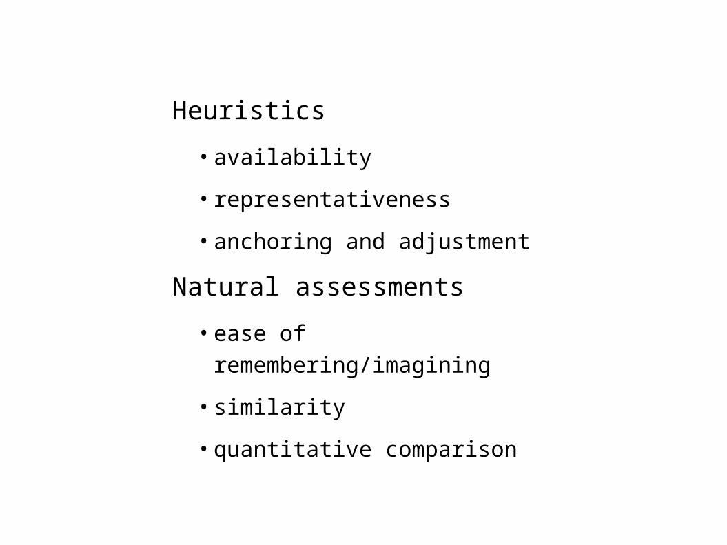
Heuristics
• availability
• representativeness
• anchoring and adjustment
Natural assessments
• ease of remembering/imagining
• similarity
• quantitative comparison

Availability: the ease with which instances are brought to mind

Which is more common?
Suicides
or
Murders?

Four Groups of Subjects
_ _ _ _ _n_
_ _ _ _ ing
Produce in 60 seconds Estimate how many in 4 pages

Four Groups of Subjects
_ _ _ _ _n_
_ _ _ _ ing
Produce in 60 seconds Estimate how many in 4 pages
2.9
6.4
4.7
13.7

Representativeness: the degree to which an instance is characteristic of a
category

Two Groups of Subjects asked:
What is more representative of Hollywood actress:
-- to be divorced 4 or more times
-- to vote Democratic
What is more probable of Hollywood actress:
-- to be divorced 4 or more times
-- to vote Democratic

Two Groups of Subjects asked:
What is more representative of Hollywood actress:
65% chose to be divorced 4 or more times
What is more probable of Hollywood actress:
83% chose to vote Democratic

Representativeness
-- does not obey extensionality
-- does not entail counting instances
-- not bounded by frequency or class inclusion

Probability and Representativeness
-- Under right circumstances, people distinguish them
-- Under other circumstances, people use representativeness to judge probability (“attribute substitution” – Kahneman and Frederick, 2002)

Bill is 34 years old. He is intelligent, but unimaginative, compulsive, and generally lifeless. In school, he was strong in mathematics but weak in social studies and humanities.

Bill is 34 years old. He is intelligent, but unimaginative, compulsive, and generally lifeless. In school, he was strong in mathematics but weak in social studies and humanities.
Bill is a physician who plays poker for a hobby.
Bill is an architect.
Bill is an accountant (A).
Bill plays jazz for a hobby (J).
Bill surfs for a hobby.
Bill is a reporter.
Bill is an accountant who plays jazz for a hobby (A and J).
Bill climbs mountains for a hobby.

BILL
A > A + J > J 87%

Linda is 31 years old, single, outspoken and very bright. She majored in philosophy. As a student, she was deeply concerned with issues of discrimination and social justice, and also participated in anti-nuclear demonstrations.

Linda is 31 years old, single, outspoken and very bright. She majored in philosophy. As a student, she was deeply concerned with issues of discrimination and social justice, and also participated in anti-nuclear demonstrations.
Linda is active in the feminist movement (F).
Linda is a bank teller (T).
Linda is a bank teller and is active in the feminist movement (T and F).

BILL
A > A + J > J 87%
LINDA
F > T + F > T 85%

Conjunction Rule
P(A & B) P(A) [or P(B)]<
Extension Rule
C contains A =>
P(C) greater then or equal to P(A) A
C

How robust are these violations of Conjunction Rule?
• Grad students in decision science
fail
• Only critical items
naive fail
sophisticated pass
• Give arguments, valid or invalid
naive fail
sophisticated pass with valid
• Experts with great experience -- physicians
fail
• Payoffs
fail

20 roles of die
2 G 4 R faces
You get $25 if your sequence occurs
R G R R RG R G R R RG R R R R

20 roles of die
2 G 4 R faces
You get $25 if your sequence occurs
R G R R R 35%G R G R R R 64%G R R R R 1%
Violates extensionality because every time the middle sequence happens, the first sequence also happens, but not vice versa

Availability can also lead to violations of the conjunction rule
_ _ _ _ _n_
_ _ _ _ ing
Produce in 60 seconds Estimate how many in 4 pages
2.9
6.4
4.7
13.7

Causality and the Conjunction Rule
Causal stories make events easier to imagine – an instance of availability

Two groups of students asked to estimate probability of:

Massive flood somewhere in North America in which more than 1000 people drown
An earthquake in California causing a flood in which more than 1000 people drown
(A. Tverksy, and Kahneman, 1982)

Massive flood somewhere in North America in which more than 1000 people drown
2.2 %
An earthquake in California causing a flood in which more than 1000 people drown
3.1%
(A. Tverksy and Kahneman,
1982)

Two groups of forecasting experts asked to estimate probability of:

A complete suspension of diplomatic relations between USA and USSR sometime in 1983
A Russian invasion of Poland and a complete suspension of diplomatic relations between USA and USSR sometime in 1983

A complete suspension of diplomatic relations between USA and USSR sometime in 1983
.14%
A Russian invasion of Poland and a complete suspension of diplomatic relations between USA and USSR sometime in 1983
.47%

Conjunction error produced by different heuristics:
Availability: search set of A and B may be better than search set of A
• Causality: A and B may be better motivated than A alone
Representativeness: A and B may be more representative than A alone

Like perceptual illusions, these cognitive illusions
-- Are difficult to get rid of
-- Seem right and compelling even when error revealed

The Muller-Lyer Illusion

To eliminate the illusion, we need to frame the problem correctly

One more heuristic: Anchoring and Adjustment
Compare quantity to another salient quantity, adjust upward or downward

Study of Anchoring (Tversky and Kahneman, 1974)
• Ps asked to estimate various quantities, e.g. percentage of African countries in the United Nations)
• For each quantity, a number between 0 and 100 was determined by spinning a wheel in Ps presence
• Ps estimate value of target quantity
– Average 25 if wheel number is 10
– Average 45 if wheel number is 65
– Payoffs for accuracy did not reduce effect
• Interpretation: Ps “anchor” on a presented quantity in making their estimate, even when it is clearly irrelevant to the task

La Rochefoucald
“Everyone complains of his memory and no one complains of his judgement”

An application of representativeness: the “hot hand in basketball”
(Gilovich, Vallone, and Tversky, 1985)
• Players and coaches in the NBA believe it is important to pass the ball to a player who has had made a streak of baskets
• They believe, specifically P(Hitnext|Hitlast) > P(Hitnext|Missedlast) for an individual player
• Careful tests show that this inequalilty does not hold; if anything, P(Hitnext|Hitlast) is slightly lower than P(Hitnext|Missedlast); same true for longer streaks
• Conclusion: There is no such thing as the “hot hand”, but belief that short sequences will be representative of long-run averages causes people to believe in it
• Very difficult to extinguish!

Another application:The iPod Shuffle

Decision Making
The psychology of choice

Assumptions of Neoclassical Economics (“Homo Economicus”)
Selfishness – an individual chooses on the basis of his/her own interests (no true, systematic altruism)
Stable, exogenous preferences – what the individual wants is well-defined, available to introspection, and stable over time
Formal rationality – an individual’s preferences, tastes, etc. are consistent with each other

Rational Choice Theories for Individuals
Utility theory – one agent, choice depends only on states of nature

Example: A decision that depends on states of nature
Options: Plan picnic outdoors Plan picnic indoors
Possible states of nature Rain No rain
Choice depends on likelihood of rain, relative quality of picnic indoors/outdoors with and without rain

Rational Choice Theories for Individuals (Von Neumann and
Morgenstern, 1944)
Utility theory – one agent, choice depends only on states of nature
Game theory – more than one agent, choice depends on what other agents may choose

Example: a decision that depends on what others may do
Options: Go to the beach Go to the cinema
Your friend may choose to: Go to the beach Go to the cinema
You cannot control or know what your friend will do Both of you know each other’s preferences Choice depends on what you think your friend will do, which
depends on what s/he thinks you will do, and so on…

Expected Utility Theory – Crucial Features
Utility (“degree of liking”) is defined by (revealed) preferences i.e. U(A) > U(B) iff A is preferred to (chosen over)
B

Expected Utility Theory – Crucial Features
Utility (“degree of liking”) is defined by (revealed) preferences i.e. U(A) > U(B) iff A is preferred to (chosen over)
B Preferences are well ordered
i.e. transitive: If A ≻ B and B ≻ C, then A ≻ C

Expected Utility Theory – Crucial Features
Utility (“degree of liking”) is defined by (revealed) preferences i.e. U(A) > U(B) iff A is preferred to (chosen over) B
Preferences are well ordered i.e. transitive: If A ≻ B and B ≻ C, then A ≻ C
Choices under uncertainty are determined by expected utility Expected utility is a probability-weighted combination of
the utilities of all n possible outcomes Oi

A Concave Utility Curve

Example: Application of Utility Theory
Options: Gamble (50% chance to win $100; else $0) Sure Thing (100% chance to win $50)
Expected values are the same: EV(Gamble) = (.5)($100) + (.5)($0) = $50 EV(Sure Thing) = (1)($50) = $50
But their expected utilities may still differ EU(Gamble) = .5U($100) + .5U($0) EU(Sure Thing) = U($50)

Expected utility theory says that utilities are…
Not directly observable (internal to an individual)
Not comparable across individuals Constrained by revealed preferences (i.e.
choices between gambles)

Do people’s choices obey the theory of expected utility (i.e., formal rationality)?

Expected Utility Theory – Crucial Features
Utility (“degree of liking”) is defined by (revealed) preferences i.e. U(A) > U(B) iff A is preferred to (chosen over)
B

Utility versus Preference (Lichtenstein and Slovic, 1971; 1973)
Ps given two options: P bet: 29/36 probability to win $2 $ bet: 7/36 probability to win $9
Two conditions: Choose one: Most prefer P bet Value the bets: Most value $ bet higher
Shows utility (based on cash value) is not consistent with revealed preference

Expected Utility Theory – Crucial Features
Utility (“degree of liking”) is defined by (revealed) preferences i.e. U(A) > U(B) iff A is preferred to (chosen over)
B Contradicted by preference reversal

Expected Utility Theory – Crucial Features
Utility (“degree of liking”) is defined by (revealed) preferences i.e. U(A) > U(B) iff A is preferred to (chosen over)
B Contradicted by preference reversal
Preferences are well ordered i.e. transitive: If A ≻ B and B ≻ C, then A ≻ C

Tests of Transitivity (A. Tversky, 1969)
Ps shown ratings of college applicants on three dimensions:
356081E
456678D
557275C
657872B
758469A
SocialStabilityIntelligenceApplicant
• Ps chose A over B, B over C, C over D, D over E, but……E over A (difference in intelligence outweighed)

Expected Utility Theory – Crucial Features
Utility (“degree of liking”) is defined by (revealed) preferences i.e. U(A) > U(B) iff A is preferred to (chosen over)
B Contradicted by preference reversal
Preferences are well ordered i.e. transitive: If A ≻ B and B ≻ C, then A ≻ C Contradicted by three-option intransitivities (and
preference reversals)

Expected Utility Theory – Crucial Features
Utility (“degree of liking”) is defined by (revealed) preferences i.e. U(A) > U(B) iff A is preferred to (chosen over) B Contradicted by preference reversals
Preferences are well ordered i.e. transitive: If A ≻ B and B ≻ C, then A ≻ C Contradicted by three-option intransitivities (and preference reversals)
Choices under uncertainty are determined by expected utility Expected utility is a probability-weighted combination of the utilities of
all n possible outcomes Oi

Testing Expected Utility (Tversky and Kahneman, 1981)
Choose between A. Sure win of $30 B. 80% chance to win $45

Testing Expected Utility (Tversky and Kahneman, 1981)
Choose between: A. Sure win of $30 B. 80% chance to win $45
Choose between: C. 25% chance to win $30 D. 20% chance to win $45

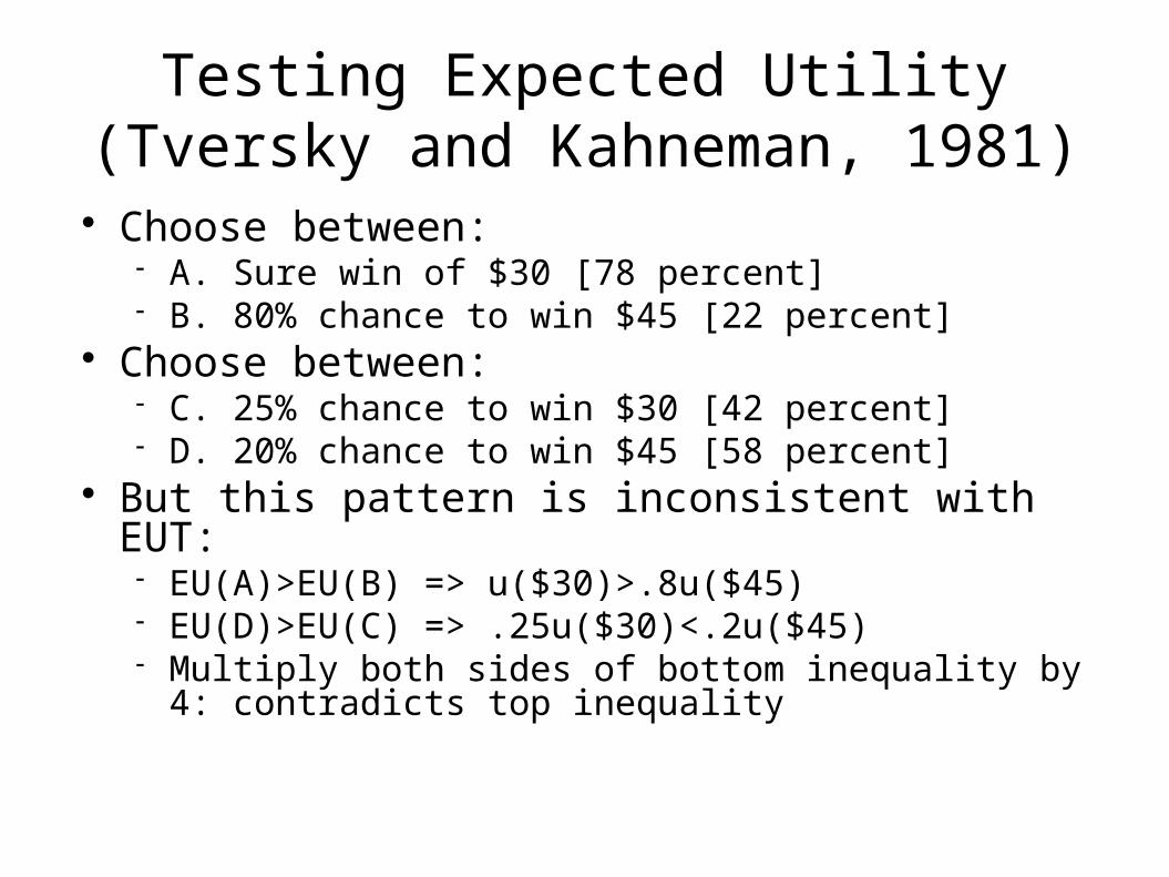
Testing Expected Utility (Tversky and Kahneman, 1981)
Choose between: A. Sure win of $30 [78 percent] B. 80% chance to win $45 [22 percent]
Choose between: C. 25% chance to win $30 [42 percent] D. 20% chance to win $45 [58 percent]
Testing Expected Utility (Tversky and Kahneman, 1981)
Choose between: A. Sure win of $30 [78 percent] B. 80% chance to win $45 [22 percent]
Choose between: C. 25% chance to win $30 [42 percent] D. 20% chance to win $45 [58 percent]
But this pattern is inconsistent with EUT: EU(A)>EU(B) => u($30)>.8u($45) EU(D)>EU(C) => .25u($30)<.2u($45) Multiply both sides of bottom inequality by 4: contradicts
top inequality

Testing Expected Utility (Tversky and Kahneman, 1981)
Choose between: A. Sure win of $30 [78 percent] B. 80% chance to win $45 [22 percent]
Choose between: C. 25% chance to win $30 [42 percent] D. 20% chance to win $45 [58 percent]
But this pattern is inconsistent with EUT: EU(A)>EU(B) => u($30)>.8u($45) EU(D)>EU(C) => .25u($30)<.2u($45) Multiply both sides of bottom inequality by 4: contradicts top inequality
This is called a “certainty effect”: certain gains have extra psychological value

Expected Utility Theory – Crucial Features
Utility (“degree of liking”) is defined by (revealed) preferences i.e. U(A) > U(B) iff A is preferred to (chosen over) B Contradicted by preference reversals
Preferences are well ordered i.e. transitive: If A ≻ B and B ≻ C, then A ≻ C Contradicted by three-option intransitivities (and preference reversals)
Choices under uncertainty are determined by expected utility Expected utility is a probability-weighted combination of the utilities of
all n possible outcomes Oi
Contradicted by certainty effect

So, people’s choices do not obey formal rationality.
Are their preferences nonetheless stable?

Neoclassical Assumptions About Preferences
The chosen option in a decision problem should remain the same even if the surface description of the problem changes (descriptive invariance)

A Test of Descriptive Invariance (Tversky and Kahneman, 1981)
Consider a two-stage game. In the first stage, there is a 75% chance to end the game without winning anything, and a 25% chance to move into the second stage. If you reach the second stage, you have a choice between Sure win of $30 80% chance to win $45
Your choice must be made before the game starts, i.e. before the outcome of the first stage is known

A Test of Descriptive Invariance (Tversky and Kahneman, 1981)
Consider a two-stage game. In the first stage, there is a 75% chance to end the game without winning anything, and a 25% chance to move into the second stage. If you reach the second stage, you have a choice between Sure win of $30 [74 percent] 80% chance to win $45 [26 percent]
Your choice must be made before the game starts, i.e. before the outcome of the first stage is known

A Test of Descriptive Invariance (continued)
But this gamble is formally identical to a problem we saw earlier, namely: Choose between:
C. 25% chance to win $30 [42 percent] D. 20% chance to win $45 [58 percent]

A Test of Descriptive Invariance (continued)
But this gamble is formally identical to a problem we saw earlier, namely: Choose between:
C. 25% chance to win $30 [42 percent] D. 20% chance to win $45 [58 percent]
Compare: Consider a two-stage game. In the first stage, there is a
75% chance to end the game without winning anything, and a 25% chance to move into the second stage. If you reach the second stage, you have a choice between
Sure win of $30 [74 percent] 80% chance to win $45 [26 percent]

A Test of Descriptive Invariance (continued)
But this gamble is formally identical to a problem we saw earlier, namely: Choose between:
C. 25% chance to win $30 [42 percent] D. 20% chance to win $45 [58 percent]
Compare: Consider a two-stage game. In the first stage, there is a 75% chance to end
the game without winning anything, and a 25% chance to move into the second stage. If you reach the second stage, you have a choice between
Sure win of $30 [74 percent] 80% chance to win $45 [26 percent]
A violation of descriptive invariance This is known as a “pseudo-certainty” effect: When a stage of the problem
is presented as involving a certain gain, it carries extra weight even if getting to that stage is itself uncertain.

Framing Effects (Tversky and Kahneman, 1981)
Problem 1: Imagine that the U.S. is preparing for the outbreak of an unusual Asian disease, which is expected to kill 600 people. Two alternative programs to combat the disease have been proposed. Assume that the exact scientific estimate of the consequences of the programs are as follows:
If Program A is adopted, 200 people will be saved If Program B is adopted, there is 1/3 probability that 600 people will be
saved, and 2/3 probability that no people will be saved.Which of the two programs do you favor?
Problem 2: If Program C is adopted 400 people will die If Program D is adopted there is 1/3 probability that nobody will die,
and 2/3 probability that 600 people will die.Which of the two programs do you favor?

Framing Effects (Tversky and Kahneman, 1981)
Problem 1: Imagine that the U.S. is preparing for the outbreak of an unusual Asian disease, which is expected to kill 600 people. Two alternative programs to combat the disease have been proposed. Assume that the exact scientific estimate of the consequences of the programs are as follows:
If Program A is adopted, 200 people will be saved [72 percent] If Program B is adopted, there is 1/3 probability that 600 people will be
saved, and 2/3 probability that no people will be saved. [28 percent] Problem 2:
If Program C is adopted 400 people will die [22 percent] If Program D is adopted there is 1/3 probability that nobody will die,
and 2/3 probability that 600 people will die. [78 percent] But the programs are identical! This example also violates descriptive
invariance. Shows reflection effect: Risk aversion in the domain of gains; risk seeking
in the domain of losses

Neoclassical Assumptions About Preferences
The chosen option in a decision problem should remain the same even if the surface description of the problem changes (descriptive invariance) Contradicted by pseudo-certainty and framing
effects

Neoclassical Assumptions About Preferences
The chosen option in a decision problem should remain the same even if the surface description of the problem changes (descriptive invariance) Contradicted by pseudo-certainty and framing effects
The chosen option should depend only on the outcomes that will obtain after the decision is made, not on differences between those outcomes and the status quo what one expects the overall magnitude of the decision

Status Quo Bias (Kahnemen, Knetsch, and Thaler, 1990)
“Sellers” each given coffee mug, asked how much they would sell if for
“Buyers” not given mug, asked how much they would pay for one
Median values: Sellers: $7.12 Buyers: $2.87

Status Quo Bias (Kahnemen, Knetsch, and Thaler, 1990)
“Sellers” each given coffee mug, asked how much they would sell if for
“Buyers” not given mug, asked how much they would pay for one
Median values: Sellers: $7.12 Buyers: $2.87
“Choosers” asked to choose between mug and cash – preferred mug if cash amount was $3.12 or lower, on average
Shows “endowment effect” – we value what we have; and “loss aversion” – we don’t want to lose it

Mental accounts and expectations (Tversky and Kahneman, 1981)
Imagine that you have decided to see a play where admission is $20 per ticket. As you enter the theater you discover that you have lost the ticket. The seat was not marked and the ticket cannot be recovered. Would you pay $20 for another ticket?

Mental accounts and expectations (Tversky and Kahneman, 1981)
Imagine that you have decided to see a play where admission is $20 per ticket. As you enter the theater you discover that you have lost a $20 bill. Would you still pay $20 for a ticket to the play?

Mental accounts and expectations (Tversky and Kahneman, 1981)
Imagine that you have decided to see a play where admission is $20 per ticket. As you enter the theater you discover that you have lost the ticket. The seat was not marked and the ticket cannot be recovered. Would you pay $20 for another ticket? [No: 54%]
Imagine that you have decided to see a play where admission is $20 per ticket. As you enter the theater you discover that you have lost a $20 bill. Would you still pay $20 for a ticket to the play? [Yes: 88%]
But in both problems, the final outcome is the same if you buy the ticket: you have the same amount of money and you see the play. Why should these cases differ?

Dependence on Ratios (Tversky and Kahneman, 1981)
Imagine that you are about to purchase a jacket for $250, and a calculator for $30. The calculator salesman informs you that the calculator [jacket] you wish to buy is on sale for $20 [$240] at the other branch of the store, located 20 minutes drive away. Would you make the trip to the other store?
Results: 68% willing to make extra trip for $30 calculator 29% willing to make extra trip for $250 jacket
Note: save same amount in both cases: $10. Why the discrepency?

Neoclassical Assumptions About Preferences
The chosen option in a decision problem should remain the same even if the surface description of the problem changes (descriptive invariance) Contradicted by pseudo-certainty and framing effects
The chosen option should depend only on the outcomes that will obtain after the decision is made, not on differences between those outcomes and the status quo: Contradicted by endowment effect what one expects: Contradicted by mental accounts the overall magnitude of the decision: Contradicted by ratio
effect

More Neoclassical Assumptions About Preferences
Preferences over future options should not depend on the transient emotional state of the decision maker at the time of the choice (state independence)
Contradicted by projection bias Preferences between future outcomes should not vary
systematically as a function of the time until the outcomes (delay independence)
Contradicted by impulsiveness Experienced utility should not differ systematically from
decision utility: Contradicted by failures of decision to predict experiences
predicted utility: Contradicted by failure to predict adaptation retrospective utility: Contradicted by duration neglect and failure to
integrate moment utilities

Prospect Theory (Kahneman and Tversky, 1979; 1992)
Prospects are evaluated according to a value function that exhibits reference dependence (subjectively oriented
around a zero point, defining gains and losses) diminishing sensitivity to differences as one moves
away from the reference point loss aversion: steeper for losses than for gains

The Value Function

Prospect Theory (Kahneman and Tversky, 1979; 1992)
Prospects are evaluated according to a value function that exhibits
reference dependence (subjectively oriented around a zero point, defining gains and losses)
diminishing sensitivity to differences as one moves away from the reference point
loss aversion: steeper for losses than for gains Probabilities are transformed by a weighting function that
exhibits diminished sensitivity to probability differences as one moves from either certainty (1.0) or impossibility (0.0) toward the middle of the probability scale (0.5)
Refinement of reflection effect: risk aversion for medium-to-high probability gains and low probability losses; risk seeking for medium to high probability losses and low probability gains

Some everyday, observed consequences of prospect theory
(Camerer, 2000) Loss aversion:
Equity premium in stock market: stock returns too high relative to bond returns Cab drivers quit around daily income target instead of “making hay while sun
shines” Most employees do not switch out of default health/benefit plans People at quarter-based schools prefer quarters, at semester-based schools
prefer semesters Reflection effect:
Horse racing: favorites underbet, longshots overbet (overweight low probability loss); switch to longshots at end of the day
People hold losing stocks too long, sell winners too early Customers buy overpriced “phone wire” insurance (overweight low probability
loss) Lottery ticket sales go up as top prize rises (overweight low probability win)

More serious consequences
Loss aversion makes individuals/societies unwilling to switch to healthier living (fear loss of income, unsustainable luxuries)
Risk seeking for likely losses can cause prolonged pursuit of doomed policies, e.g. wars that are not likely to be won, choosing court trial instead of bargaining
Risk seeking for unlikely gains can lead to excessive gambling in individuals, quixotic policies when leaders get too powerful

Okay, people are not generally rational and don’t have stable preferences, but aren’t they at least basically selfish?

Self-Interest Assumption in Game Theory
Choices in games should always reflect what is best for the decision maker, i.e. what will maximize the decision maker’s payoff

Prisoner’s Dilemma (Tucker, 1955)

Prisoner’s Dilemma Labeling Experiment (Ross and Samuels, 1993)
When PD is labeled the “Wall Street Game”, only 1/3 cooperate
When it is labeled the “Community Game”, 2/3 cooperate
Shows presence of both tendencies – defection and cooperation – which can be evoked by social signals

The Ultimatum Game (Guth et al., 1982)
$100 in one dollar bills available to be divided between two players
“Proposer” chooses a division “Receiver” can either
accept: both receive proposed amounts reject: both receive nothing
How much should the Proposer offer?

The Ultimatum Game (Guth et al., 1982)
$10 in one dollar bills available to be divided between two players
“Proposer” chooses a division “Receiver” can either
accept: both receive proposed amounts reject: both receive nothing
How much should the Proposer offer?

Ultimatum game experiment (Thaler, 1988)
Most proposers offer $5 (even split), or a little less, to the receiver altruism
Low offers ($1) usually rejected “altruistic punishment”

Dictator Game (Kahneman et al., 1986)
One P (student in class) asked to divide $20 between self and other P. Other P has no choice to accept/reject.
Two possibilities: Even split ($10 each) Uneven split ($18 for self, $2 for other)
Game theory predicts uneven split 76% chose an even split

Ultimatum and Dictator Games in Traditional Societies (Henrich et al.,
2001) Ps tested 15 small-scale societies Ultimatum game:
Mean offer varied from 0.26 to 0.58 (0.44 in industrial societies)
Rejection rate also quite varied: low offers rarely rejected in some groups, in others high offers are often rejected
Great variation in behavior even among nearby groups; depends on deep aspects of culture, experience: e.g. meat-sharing Ache (Paraguay) and village-minded
Orma (Kenya) made generous offers, family-focused Machiguenga (Peru) showed low cooperation

Ultimatum and Dictator Games in Traditional Societies (Henrich et al.,
2001) Ps tested 15 small-scale societies Ultimatum game:
Mean offer varied from 0.26 to 0.58 (0.44 in industrial societies) Rejection rate also quite varied: low offers rarely rejected in some
groups, in others high offers are often rejected Great variation in behavior even among nearby groups;
depends on deep aspects of culture, experience: e.g. meat-sharing Ache (Paraguay) and village-minded Orma (Kenya)
made generous offers, family-focused Machiguenga (Peru) showed low cooperation
General conclusion: there is no such thing as homo economicus; cooperation behavior is highly variable, heavily determined by cultural norms

Are people generally rational? People evolved to cope with problems the brain
has faced for most of humanity's existence (i.e. pre-civilizational) – for these problems, the brain could be considered well-adapted, but it can still be fooled
The modern world of commerce, technology, and politics presents challenges to which the brain is not well adapted
Behavior is not well described by formal theories of rationality: probability, decision and game theory