JUAS12_02- P.J. Bryant- Lecture 2 ‘Hard-edge’ model & Transverse motion in Magnetic elements - Slide 1 ‘HARD-EDGE’ MODEL & TRANSVERSE MOTION in MAGNETIC

JUAS12_02- P.J. Bryant- Lecture 2 ‘Hard-edge’ model & Transverse motion in Magnetic elements - Slide 1

‘HARD-EDGE’ MODEL&

TRANSVERSE MOTIONin

MAGNETIC ELEMENTS

Lecture 2January 2012

P.J. Bryant


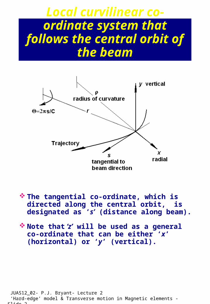
Local curvilinear co-ordinate system that follows the central

orbit of the beam

The tangential co-ordinate, which is directed along the central orbit, is designated as ‘s’ (distance along beam).

Note that ‘z’ will be used as a general co-ordinate that can be either ‘x’ (horizontal) or ‘y’ (vertical).


Terminology In general, an accelerator lattice comprises a series of

magnetic and/or electrostatic and/or electromagnetic elements separated by field-free, drift spaces.

In most cases, the lattice is dominated by magnetic dipoles and quadrupoles that constitute what is called the linear lattice. Quadrupole and higher-order lenses are usually centred on the orbit and do not affect the geometry of the accelerator.

The trajectory followed by the reference ion is known as the central orbit or equilibrium.

In a ‘ring’ lattice, the enforced periodicity defines the equilibrium orbit unambiguously and obliges it to be closed. For this reason, it is often called the closed orbit. In transfer lines, there is an extra degree of freedom and the designer is required to specify a point on the 6-dimensional (x, x′, y, y′, s, dp/p) trajectory.

Ions of the same momentum as the reference ion, but with small spatial deviations will oscillate about the equilibrium orbit with what are known as betatron oscillations.

Ions with a different momentum will have a different equilibrium orbit that will be referred to as an off-momentum or off-axis equilibrium orbit. Off-momentum ions with small spatial errors will perform betatron oscillations about their off-momentum equilibrium orbit.


Modeling

An exact determination of the equilibrium orbit and the focusing along that orbit are difficult, if not impossible.

Measuring the beam position in an existing lattice or tracking through a field map are both techniques of limited precision.

To make calculations more tractable, while still providing a reasonably accurate picture, the ‘hard-edge’ magnet model has been developed.

It is sometimes forgotten that virtually the whole of lattice optics rests on the very sweeping assumption that a useful representation of reality can be obtained from the ‘hard-edge’ model.


‘Hard-edge’ model

The ‘hard-edge’ model: Replaces dipoles, quadrupoles and solenoids by

'blocks' of field that are uniform in the axial direction within the block and zero outside the block.

Replaces multipole lenses, above quadrupole, by point kicks.

Makes the link to the real-world by equating the field integral in the model to the field integral in the real-world magnet.

Firstly, this model must respect Maxwell’s Equations to ensure that phase space is conserved and the model violates no fundamental principles.

Secondly, the pseudo-harmonic oscillations of the beam, called betatron oscillations, should have a wavelength that is much longer than the fringe-field regions. This factor determines the level of convergence between what the model predicts and what actually occurs.

In some instances, fringe-field corrections may be applied to improve this agreement.

Cyclotron motion in the uniform blocks of dipole field underpins the geometry of the ‘hard-edge’ model.


In general, the central orbit is very simple

Example racetrack lattice with two 180 degree dipoles and various quadrupoles and sextupoles.

Central orbit is straight through the centres of the lenses and semi-circular in each dipole.


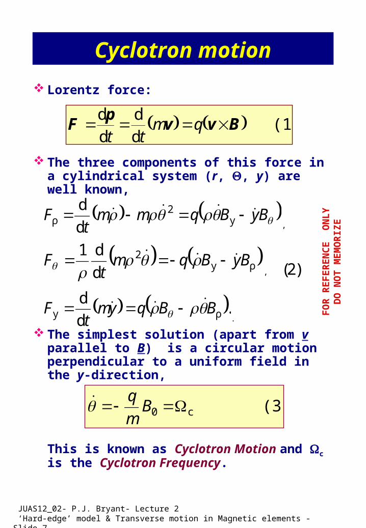
Cyclotron motion

Lorentz force:

The three components of this force in a cylindrical system (r, , y) are well known,

The simplest solution (apart from v parallel to B) is a circular motion perpendicular to a uniform field in the y-direction,

This is known as Cyclotron Motion and c is the Cyclotron Frequency.

(1) dd

dd

Bvvp

F qmtt

ByBqmmt

F y2

ρ d

d,

ρy2

d

d1ByBqm

tF

, (2)

.d

dρy BBqym

tF

.

(3) c0 Bm

q

FO

R R

EF

ER

EN

CE

ON

LY

D

O N

OT

ME

MO

RIZ

E


More on cyclotron motion

Or more simply, equate expressions for the centripetal force:

This leads to a universally-used ‘engineering’ formula, which relates the momentum of the ion to its Magnetic Rigidity, or reluctance to be deviated by the magnetic field.

where q = ne, A is the atomic mass number and p is the average momentum per nucleon so that Ap = mv0.

Since the formula is based on momentum, the non-linear effects of relativity are hidden. Note that the application of a sign convention is avoided by making the rigidity and the momentum positive and that the units are specified in the equation.

(4) 0

20

00 mv

Bqv

(5) GeV/c3356.3

Tm00 pAn

B


Cyclotron motion and bending

Cyclotron motion leads to a second universally-used ‘engineering’ formula, which relates the bending of the ion trajectory to its Magnetic Rigidity.

Note that the sign convention is again avoided and that the units are included.

Summary:The ‘hard-edge’ model is used for almost all

lattice calculations. In this model, the central or equilibrium orbit

is a stepwise progression of straight sections and circular arcs of cyclotron motion.

For a singly-charged particle (5) simplifies to,

To derive the angle formula,

(6) Tm

]m[d[T]rad

00

B

sB

GeV/c3356.3Tm00 pB

B

sB

B

B d


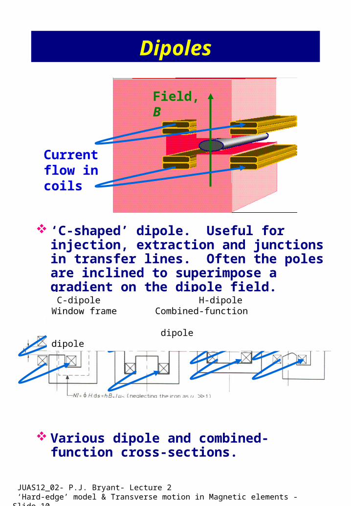
Dipoles

‘C-shaped’ dipole. Useful for injection, extraction and junctions in transfer lines. Often the poles are inclined to superimpose a gradient on the dipole field.

Various dipole and combined-function cross-sections.

Field, B

Current flow in coils

C-dipole H-dipole Window frame Combined-function dipole dipole


Transverse motion

The transverse ion motion in the lattice will be described by small perturbations from the central orbit that comprises a stepwise progression of straight sections and segments of cyclotron motion.

The transverse motion will be derived in a local curvilinear co-ordinate system (x, y, s) that follows the central orbit.

The student will find the following derivations in various forms throughout the literature and, no doubt, elsewhere in this course. The result is a classic one and the repetition is intended to help with understanding.


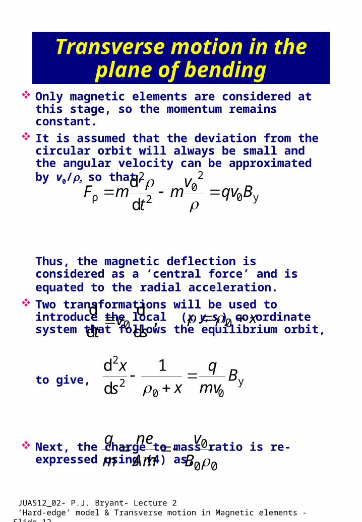
Transverse motion in the plane of bending

Only magnetic elements are considered at this stage, so the momentum remains constant.

It is assumed that the deviation from the circular orbit will always be small and the angular velocity can be approximated by v0/so that,

Thus, the magnetic deflection is considered as a ‘central force’ and is equated to the radial acceleration.

Two transformations will be used to introduce the local (x, y, s,) co-ordinate system that follows the equilibrium orbit,

to give,

Next, the charge to mass ratio is re-expressed using (4) as,

y0

20

2

2

ρd

dBqv

vm

tmF

, dd

dd

0 sv

t x 0

y00

2

2 1

d

dB

mvq

xs

x

00

0

B

v

mAne

mq


Transverse motion in the plane of bending continued

Now expand the field in a Taylor series up to the quadrupole component,

where

k is the normalised gradient. Note that the sign convention chosen introduces a ‘minus’. In other lectures, you will surely see a ‘plus’ sign and a different right-handed co-ordinate system. Welcome to two differences that you will find throughout the literature.

Substituting for the field and remembering that x<< gives,

xkBBxx

BBB

0

0

y0y

(7) 1

0

y

x

B

Bk

(8) 01

d

d2

02

2

xk

s

x


Comments on the derivation

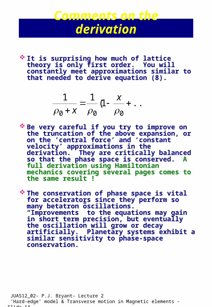
It is surprising how much of lattice theory is only first order. You will constantly meet approximations similar to that needed to derive equation (8).

Be very careful if you try to improve on the truncation of the above expansion, or on the ‘central force’ and ‘constant velocity’ approximations in the derivation. They are critically balanced so that the phase space is conserved. A full derivation using Hamiltonian mechanics covering several pages comes to the same result !

The conservation of phase space is vital for accelerators since they perform so many betatron oscillations. “Improvements” to the equations may gain in short term precision, but eventually the oscillation will grow or decay artificially. Planetary systems exhibit a similar sensitivity to phase-space conservation.

....)1(11

000

x

x


Comments continued

Note that the theory is based on a hard-edge model of a sector dipole that looks in plan view like,

However, we often have rectangular dipoles. These require some extra treatment, known as edge focusing. Edge focusing is not treated here.

Central orbit

Sector dipole

Note orbit perpendicular to magnet face

Rectangular dipole

Note The orbit is NOT perpendicular to the magnet face


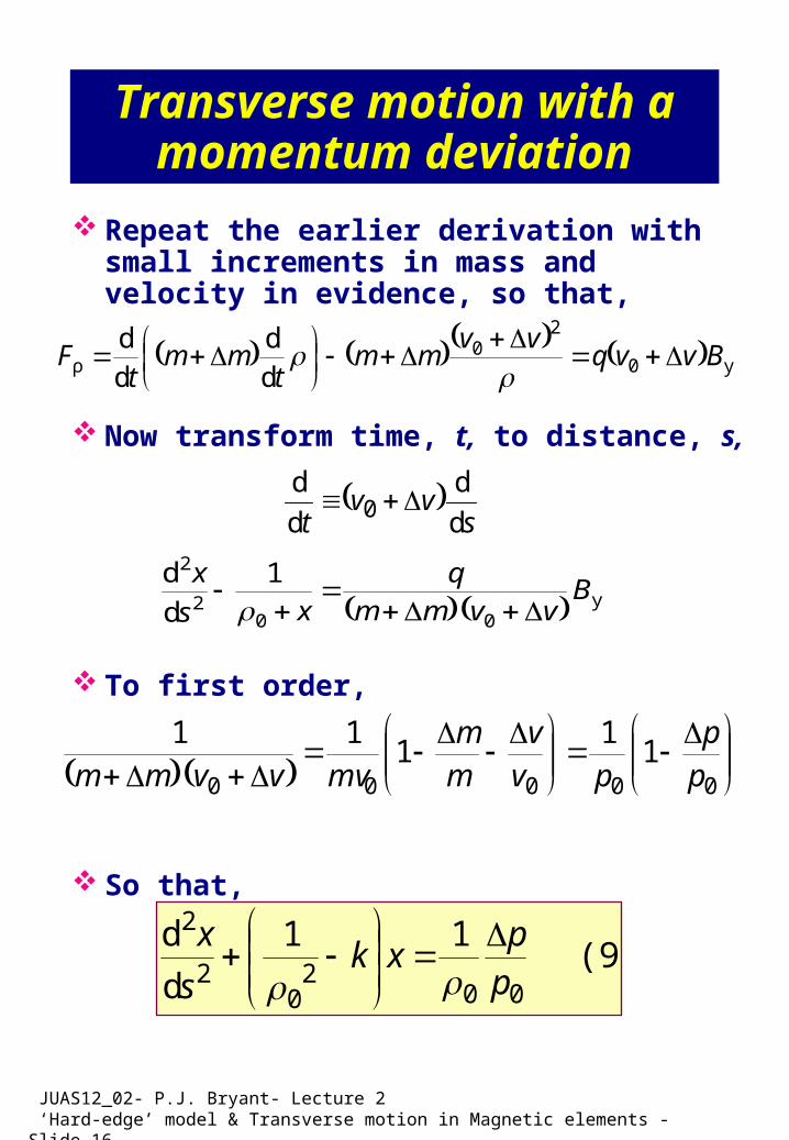
Transverse motion with a momentum deviation

Repeat the earlier derivation with small increments in mass and velocity in evidence, so that,

Now transform time, t, to distance, s,

To first order,

So that,

y0

20

ρ dd

dd

Bvvqvv

mmt

mmt

F

y00

2

2 1

d

dB

vvmmq

xs

x

00000

11

111

p

p

pv

v

m

m

mvvvmm

(9) 11

d

d

002

02

2

pp

xks

x

s

vvt d

d

d

d0


Transverse motion in the plane perpendicular to bending

Basically the analysis is repeated, except that the magnetic field has a different form,

Remember that to first order,

which gives,

.d

d

d

dρ0 Bvvq

t

ymm

tFy

.d

dρ

02

2

Bvvmm

q

s

y

00000

11

111

p

p

pv

v

m

m

mvvvmm

.11

d

dρ

0002

2

Bp

p

Bs

y


Transverse motion in plane perpendicular to bending

Now expand the field and replace B by Bx,

Substitution in the motion equation gives,

But we consider the ‘y p/p’ as second order and discard it to finish with,

Note that p/p has disappeared so this equation works (to first order) for on- and off-momentum ions. The k applies to the gradient in combined-function dipoles. For a pure dipole, k = 0 and the dipole acts like a drift space.

yy

BBB x

0x

.1d

d

02

2

p

pky

s

y

)10(0d

d2

2

kys

y

0for 0x yB


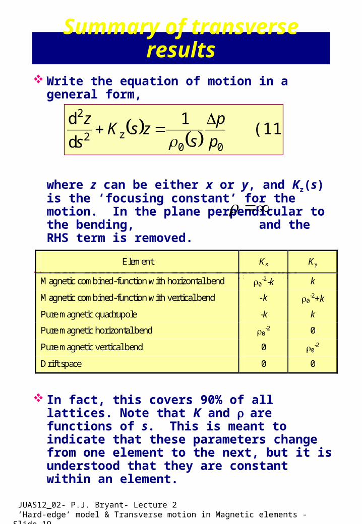
Summary of transverse results Write the equation of motion in a general form,

where z can be either x or y, and Kz(s) is the ‘focusing constant’ for the motion. In the plane perpendicular to the bending, and the RHS term is removed.

Then define what forms Ky can take:

In fact, this covers 90% of all lattices. Note that K and are functions of s. This is meant to indicate that these parameters change from one element to the next, but it is understood that they are constant within an element.

(11) 1

d

d

00z2

2

p

p

szsK

s

z

Element Kx Ky

Magnetic combined-function with horizontal bend 0-2-k k

Magnetic combined-function with vertical bend -k 0-2+k

Pure magnetic quadrupole -k k

Pure magnetic horizontal bend 0-2 0

Pure magnetic vertical bend 0 0-2

Drift space 0 0


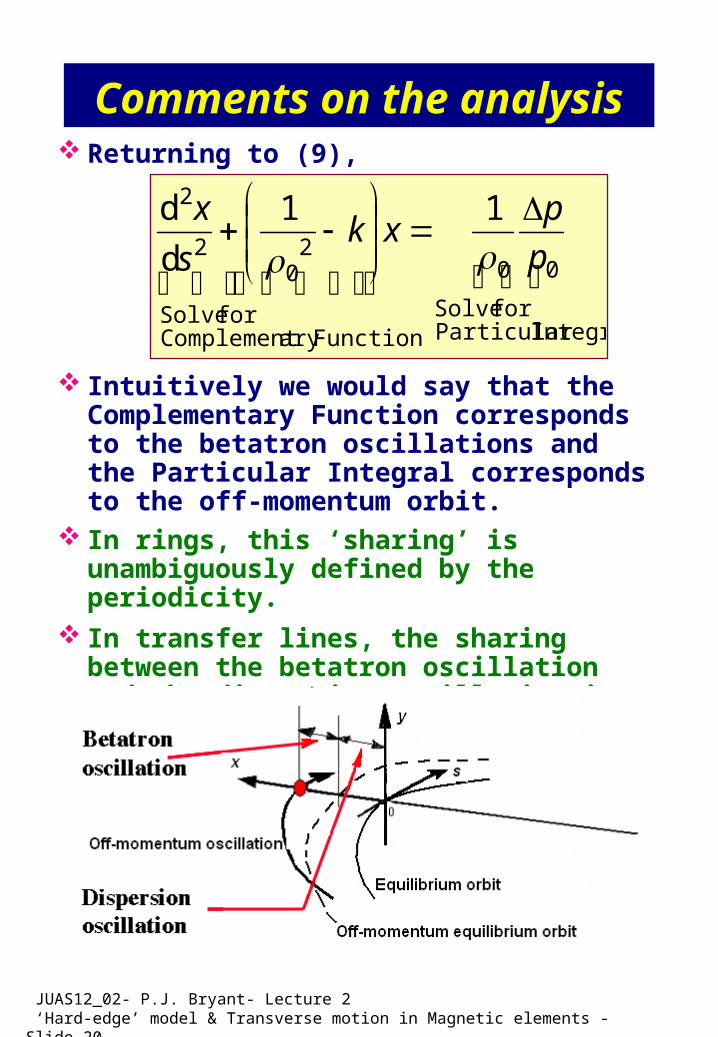
Comments on the analysis Returning to (9),

Intuitively we would say that the Complementary Function corresponds to the betatron oscillations and the Particular Integral corresponds to the off-momentum orbit.

In rings, this ‘sharing’ is unambiguously defined by the periodicity.

In transfer lines, the sharing between the betatron oscillation and the dispersion oscillation is arbitrary and must be defined by the user. We will see this again in later lectures.

Integral Particular

for Solve

00

Functionary Complementfor Solve

20

2

2 11

d

d

p

pxk

s

x


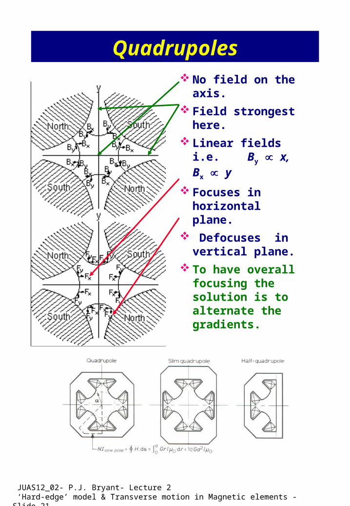
Quadrupoles No field on the axis.

Field strongest here.

Linear fields i.e. By x, Bx y

Focuses in horizontal plane.

Defocuses in vertical plane.

To have overall focusing the solution is to alternate the gradients.


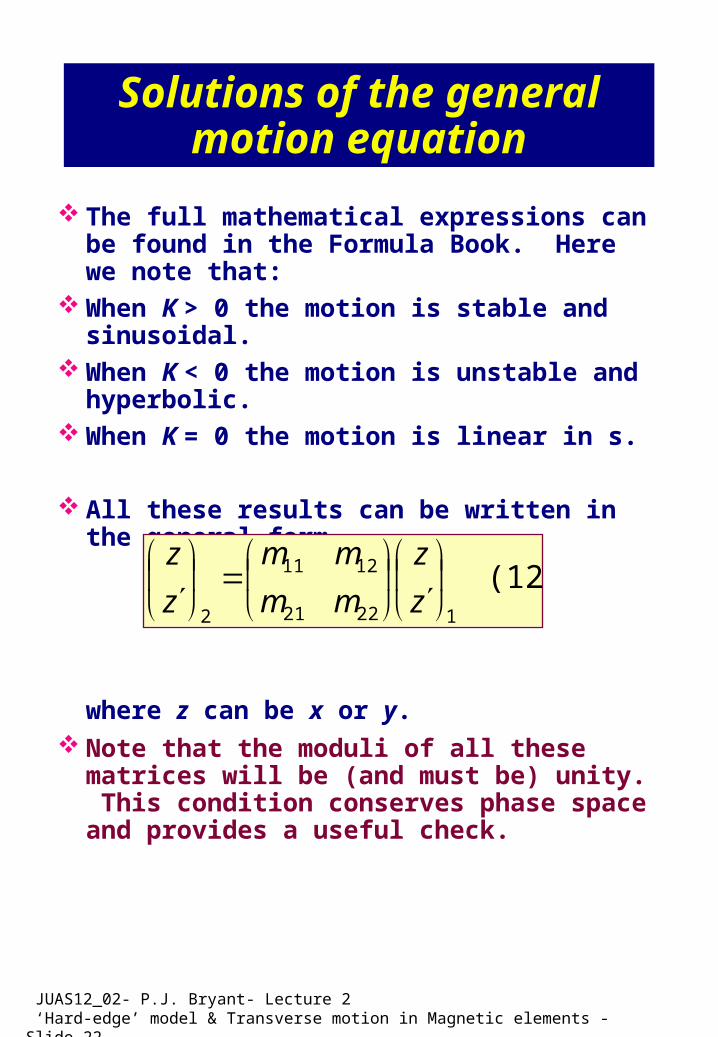
Solutions of the general motion equation

The full mathematical expressions can be found in the Formula Book. Here we note that:

When K > 0 the motion is stable and sinusoidal. When K < 0 the motion is unstable and

hyperbolic. When K = 0 the motion is linear in s.

All these results can be written in the general form

where z can be x or y. Note that the moduli of all these matrices will be

(and must be) unity. This condition conserves phase space and provides a useful check.

(12) 12221

1211

2

z

z

mm

mm

z

z


Matrices for on-momentum ions

The transfer matrix of a focusing element (K>0) is:

The transfer matrix of a defocusing element (K<0) is:

The transfer matrix of a drift space (K=0) is:

The various forms of K are given on an earlier slide.

(13) cossin

sin1

cos

KKK

KK

K

(14) coshsinh

sinh1

cosh

KKK

KK

K

(15) 10

1


Solutions of the motion equation including momentum

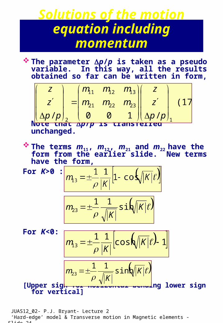
The parameter p/p is taken as a pseudo variable. In this way, all the results obtained so far can be written in form,

Note that p/p is transferred unchanged.

The terms m11, m12, m21 and m22 have the form from the earlier slide. New terms have the form,

For K>0 :

For K<0:

[Upper sign for horizontal bending lower sign for vertical]

(17)

/100/1

232221

131211

2

pp

z

z

mmm

mmm

pp

z

z

KK

m sin11

23

1cosh11

13 KK

m

KK

m sinh11

23


Calculating trajectories

Once the transfer matrices of all the elements in a lattice are known, then transfer though the lattice and to all boundaries between elements can be found by matrix multiplication.

where z can be x or y.

Note that drawings normally have the beam traveling from left to right and the matrix multiplication goes from right to left.

This method is universally used for tracking in lattices.

We now have 90% of the basic concepts for modeling and tracking.

(16)

/

....

/1

1231

pp

z

z

MMMMM

pp

z

z

nn

n

M1M2

M3

Mn-1

Mn


Summary

We have replaced all real-world dipoles and quadrupoles by uniform blocks of field.

Surprisingly, in almost all cases we are allowed to ignore fringe fields, stray flux being shunted in nearby yokes and affecting the permeability, 3D rather than 2D field distributions and so on.

We have truncated all series to linear terms only.

We have applied a ‘central force’ approach in bending regions.

We have fixed a constant axial velocity.

Finally, everything is expressed in 2 2 matrices or 3 3 matrices.

The approach is clear, simple and effective, but is also full of approximations.

It is now trivial mathematics for example to invert the matrices and back-track in a lattice.

And the way is now open to making some analytical studies of simple layouts.


Force on a current in a field

Notes for private study

Field direction around a positive current

A ‘null point’ forms where fields oppose. Force pulls current towards null point.

Right-hand rule


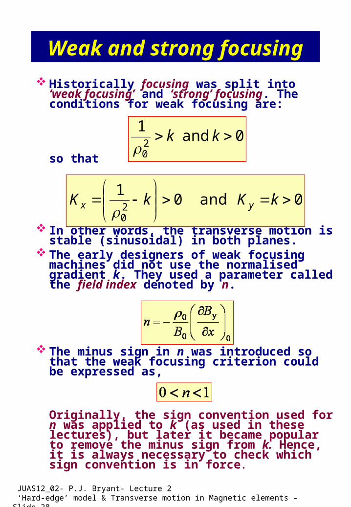
Weak and strong focusing

Historically focusing was split into ‘weak focusing’ and ‘strong’ focusing. The conditions for weak focusing are:

so that

In other words, the transverse motion is stable (sinusoidal) in both planes.

The early designers of weak focusing machines did not use the normalised gradient k. They used a parameter called the field index denoted by n.

The minus sign in n was introduced so that the weak focusing criterion could be expressed as,

Originally, the sign convention used for n was applied to k (as used in these lectures), but later it became popular to remove the minus sign from k. Hence, it is always necessary to check which sign convention is in force.

0and1

20

kk

0and01

20

kKkK yx


Thin quadrupoles

Consider equations (13) and (14) in the limit of the argument going to zero:

BUT this matrix does not have a modulus of unity! This is an example of the care we have to take with approximations.

To solve this problem put m12 = 0 but keep the integral of the gradient in term m21 to give,

which is the universally-used approximation for a thin quadrupole lens of zero length.

This extremely simple matrix with the equally simple drift-space matrix opens the way to analytical studies of quadrupole focusing schemes. It may also be a source of examination questions.

1

1 0When

k

k

1

01

k

Documents

JUAS12_02- P.J. Bryant- Lecture 2 ‘Hard-edge’ model & Transverse motion in Magnetic elements - Slide 1 ‘HARD-EDGE’ MODEL & TRANSVERSE MOTION in MAGNETIC