Embed Size (px)
Citation preview

Intro Design Metric Gradient Annealing Lab Review Conclusions
JSALT Summer School: Neural Networks
Mark Hasegawa-Johnson
University of Illinois
2015/06/23

Intro Design Metric Gradient Annealing Lab Review Conclusions
Outline
1 Intro
2 Knowledge-Based Design
3 Error Metric
4 Gradient Descent
5 Simulated Annealing
6 Lab Review
7 Conclusions

Intro Design Metric Gradient Annealing Lab Review Conclusions
Two-Layer Feedforward Neural Network
1 x1 x2 . . . xp ~x is the input vector
ak = uk0 +∑p
j=1 ukjxj ~a = U~x
1 y1 y2 . . . yq yk = f (ak) ~y = f (~a)
b` = vk0 +∑q
k=1 v`kyk ~b = V ~y
z1 z2 . . . zr z` = g(b`) ~z = g(~b)
~z = h(~x ,U,V )

Intro Design Metric Gradient Annealing Lab Review Conclusions
Neural Network = Universal Approximator
Assume. . .
Linear Output Nodes: g(b) = b
Smoothly Nonlinear Hidden Nodes: f ′(a) = dfda finite
Smooth Target Function: ~z = h(~x ,U,V ) approximates~ζ = h∗(~x) ∈ H, where H is some class of sufficiently smoothfunctions of ~x (functions whose Fourier transform has a firstmoment less than some finite number C )
There are q hidden nodes, yk , 1 ≤ k ≤ q
The input vectors are distributed with some probability densityfunction, p(~x), over which we can compute expected values.
Then (Barron, 1993) showed that. . .
maxh∗(~x)∈H
minU,V
E[h(~x ,U,V )− h∗(~x)|2
]≤ O
{1
q
}

Intro Design Metric Gradient Annealing Lab Review Conclusions
Neural Network Problems: Outline of Remainder of this Talk
1 Knowledge-Based Design. Given U,V , f , g , what kind offunction is h(~x ,U,V )? Can we draw ~z as a function of ~x?Can we heuristically choose U and V so that ~z looks kindalike ~ζ?
2 Error Metric. In what way should ~z = h(~x) be “similar to”~ζ = h∗(~x)?
3 Local Optimization: Gradient Descent withBack-Propagation. Given an initial U,V , how do I find U,V that more closely approximate ~ζ?
4 Global Optimization: Simulated Annealing. How do I findthe globally optimum values of U and V ?

Intro Design Metric Gradient Annealing Lab Review Conclusions
Outline
1 Intro
2 Knowledge-Based Design
3 Error Metric
4 Gradient Descent
5 Simulated Annealing
6 Lab Review
7 Conclusions

Intro Design Metric Gradient Annealing Lab Review Conclusions
Synapse, First Layer: ak = uk0 +∑2
j=1 ukjxj

Intro Design Metric Gradient Annealing Lab Review Conclusions
Axon, First Layer: yk = tanh(ak)

Intro Design Metric Gradient Annealing Lab Review Conclusions
Synapse, Second Layer: b` = v`0 +∑2
k=1 v`kyk

Intro Design Metric Gradient Annealing Lab Review Conclusions
Axon, Second Layer: z` = sign(b`)

Intro Design Metric Gradient Annealing Lab Review Conclusions
Step and Logistic nonlinearities Signum and Tanh nonlinearities

Intro Design Metric Gradient Annealing Lab Review Conclusions
“Linear Nonlinearity” and ReLU Max and Softmax
Max:
z` =
{1 b` = maxm bm0 otherwise
Softmax:
z` =eb`∑m ebm

Intro Design Metric Gradient Annealing Lab Review Conclusions
Outline
1 Intro
2 Knowledge-Based Design
3 Error Metric
4 Gradient Descent
5 Simulated Annealing
6 Lab Review
7 Conclusions

Intro Design Metric Gradient Annealing Lab Review Conclusions
Error Metric: How should h(~x) be “similar to” h∗(~x)?Linear output nodes:
Minimum Mean Squared Error (MMSE)
U∗,V ∗ = arg minEn = arg min1
n
n∑i=1
|~ζi − ~z(xi )|2
MMSE Solution: ~z = E[~ζ|~x]
If the training samples (~xi , ~ζi ) are i.i.d., then
E∞ = E[|~ζ − ~z |2
]E∞ is minimized by
~zMMSE (~x) = E[~ζ|~x]
Intro Design Metric Gradient Annealing Lab Review Conclusions
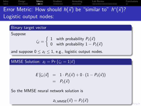
Error Metric: How should h(~x) be “similar to” h∗(~x)?Logistic output nodes:
Binary target vector
Suppose
ζ` =
{1 with probability P`(~x)0 with probability 1− P`(~x)
and suppose 0 ≤ z` ≤ 1, e.g., logistic output nodes.
MMSE Solution: z` = Pr {ζ` = 1|~x}
E [ζ`|~x ] = 1 · P`(~x) + 0 · (1− P`(~x))
= P`(~x)
So the MMSE neural network solution is
z`,MMSE (~x) = P`(~x)

Intro Design Metric Gradient Annealing Lab Review Conclusions
Error Metric: How should h(~x) be “similar to” h∗(~x)?Softmax output nodes:
One-Hot Vector, MKLD Solution: z` = Pr {ζ` = 1|~x}
Suppose ~ζi is a “one hot” vector, i.e., only one element is“hot” (ζ`(i),i = 1), all others are “cold” (ζmi = 0, m 6= `(i)).
MMSE will approach the solution z` = Pr {ζ` = 1|~x}, butthere’s no guarantee that it’s a correctly normalized pmf(∑
z` = 1) until it has fully converged.
MKLD also approaches z` = Pr {ζ` = 1|~x}, and guaranteesthat
∑z` = 1. MKLD is also more computationally efficient,
if ~ζ is a one-hot vector.
MKLD = Minimum Kullback-Leibler Distortion
Dn =1
n
n∑i=1
r∑`=1
ζ`i log
(ζ`iz`i
)= −1
n
n∑i=1
log z`(i),i

Intro Design Metric Gradient Annealing Lab Review Conclusions
Error Metrics Summarized
Use MSE to achieve ~z = E[~ζ|~x]. That’s almost always what
you want.
If ~ζ is a one-hot vector, then use KLD (with a softmaxnonlinearity on the output nodes) to guarantee that ~z is aproperly normalized probability mass function, and for bettercomputational efficiency.
If ζ` is binary, but not necessarily one-hot, then use MSE(with a logistic nonlinearity) to achieve z` = Pr {ζ` = 1|~x}.If ζ` is signed binary (ζ` ∈ {−1,+1}, then use MSE (with atanh nonlinearity) to achieve z` = E [ζ`|~x ].
After you’re done training, you can make your cell phone appmore efficient by throwing away the uncertainty:
Replace softmax output nodes with maxReplace logistic output nodes with unit-stepReplace tanh output nodes with signum

Intro Design Metric Gradient Annealing Lab Review Conclusions
Outline
1 Intro
2 Knowledge-Based Design
3 Error Metric
4 Gradient Descent
5 Simulated Annealing
6 Lab Review
7 Conclusions

Intro Design Metric Gradient Annealing Lab Review Conclusions
Gradient Descent = Local Optimization

Intro Design Metric Gradient Annealing Lab Review Conclusions
Gradient Descent = Local Optimization
Given an initial U,V , find U, V with lower error.
ukj = ukj − η∂En
∂ukj
v`k = v`k − η∂En
∂v`k
η =Learning Rate
If η too large, gradient descent won’t converge. If too small,convergence is slow. Usually we pick η ≈ 0.001 and cross ourfingers.
Second-order methods like L-BFGS choose an optimal η ateach step, so they’re MUCH faster.

Intro Design Metric Gradient Annealing Lab Review Conclusions
Computing the Gradient
OK, let’s compute the gradient of En with respect to the Vmatrix. Remember that V enters the neural net computation asb`i =
∑k v`kyki , and then z depends on b somehow. So. . .
∂En
∂v`k=
n∑i=1
(∂En
∂b`i
)(∂b`i∂v`k
)
=n∑
i=1
ε`iyki
where the last line only works if we define ε`i in a useful way:
Back-Propagated Error
ε`i =∂En
∂b`i=
2
n(z`i − ζ`i )g ′(b`i )
where g ′(b) = ∂g∂b .

Intro Design Metric Gradient Annealing Lab Review Conclusions
1 x1 x2 . . . xp ~x is the input vector
ak = uk0 +∑p
j=1 ukjxj ~a = U~x
1 y1 y2 . . . yq yk = f (ak) ~y = f (~a)
b` = vk0 +∑q
k=1 v`kyk ~b = V ~y
z1 z2 . . . zr z` = g(b`) ~z = g(~b)
~z = h(~x ,U,V )
Back-Propagating to the First Layer
∂En
∂ukj=
n∑i=1
(∂En
∂aki
)(∂aki∂ukj
)=
n∑i=1
δkixji
where. . . δki =∂En
∂aki=
r∑`=1
ε`iv`k f′(aki )

Intro Design Metric Gradient Annealing Lab Review Conclusions
The Back-Propagation Algorithm
V = V − η∇VEn, U = U − η∇UEn
∇VEn = EY T , ∇UEn = DXT
Y = [~y1, . . . , ~yn] , X = [~x1, . . . , ~xn]
E = [~ε1, . . . ,~εn] , D =[~δ1, . . . , ~δn
]~εi =
2
ng ′(~bi )�
(~zi − ~ζi
), ~δi = f ′(~ai )� V T~εi
. . . where � means element-wise multiplication of two vectors;g ′(~b) and f ′(~a) are element-wise derivatives of the g(·) and f (·)nonlinearities.

Intro Design Metric Gradient Annealing Lab Review Conclusions
Derivatives of the Nonlinearities
Logistic Tanh ReLU

Intro Design Metric Gradient Annealing Lab Review Conclusions
Outline
1 Intro
2 Knowledge-Based Design
3 Error Metric
4 Gradient Descent
5 Simulated Annealing
6 Lab Review
7 Conclusions

Intro Design Metric Gradient Annealing Lab Review Conclusions
Simulated Annealing: How can we find the globallyoptimum U ,V ?
Gradient descent finds a local optimum. The U, V you end upwith depends on the U,V you started with.
How can you find the global optimum of a non-convex errorfunction?
The answer: Add randomness to the search, in such a waythat. . .
P(reach global optimum)t→∞−→ 1

Intro Design Metric Gradient Annealing Lab Review Conclusions
Take a random step. If it goes downhill, do it.

Intro Design Metric Gradient Annealing Lab Review Conclusions
Take a random step. If it goes downhill, do it.
If it goes uphill, SOMETIMES do it.
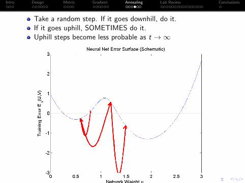
Intro Design Metric Gradient Annealing Lab Review Conclusions
Take a random step. If it goes downhill, do it.If it goes uphill, SOMETIMES do it.Uphill steps become less probable as t →∞

Intro Design Metric Gradient Annealing Lab Review Conclusions
Simulated Annealing: Algorithm
FOR t = 1 TO ∞, DO
1 Set U = U + RANDOM
2 If your random step caused the error to decrease(En(U) < En(U)), then set U = U(prefer to go downhill)
3 Else set U = U with probability P(. . . but sometimes go uphill!)
1 P = exp(−(En(U)− En(U))/Temperature)(Small steps uphill are more probable than big stepsuphill.)
2 Temperature = Tmax/ log(t + 1)(Uphill steps become less probable as t →∞.)
4 Whenever you reach a local optimum (U is better than boththe preceding and following time steps), check to see if it’sbetter than all preceding local optima; if so, remember it.

Intro Design Metric Gradient Annealing Lab Review Conclusions
Convergence Properties of Simulated Annealing
(Hajek, 1985) proved that, if we start out in a “valley” that isseparated from the global optimum by a “ridge” of height Tmax ,and if the temperature at time t is T (t), then simulated annealingconverges in probability to the global optimum if
∞∑t=1
exp (−Tmax/T (t)) = +∞
For example, this condition is satisfied if
T (t) = Tmax/ log(t + 1)

Intro Design Metric Gradient Annealing Lab Review Conclusions
Outline
1 Intro
2 Knowledge-Based Design
3 Error Metric
4 Gradient Descent
5 Simulated Annealing
6 Lab Review
7 Conclusions

Intro Design Metric Gradient Annealing Lab Review Conclusions
Here’s the dataset

Intro Design Metric Gradient Annealing Lab Review Conclusions
You’ll have to plot it many times, so I recommend writing a plotfunction
function ER = nnplot(X,Z,ZETA,STRING,fignum)
[p,n]=size(X);
ER=sum(ZETA.*Z<0)/n;
figure(fignum);
plot(X(1,Z<0),X(2,Z<0),’r.’,X(1,Z>0),X(2,Z>0),’b.’);
title(sprintf(’WS15 ANN Lab, %s, ER=%g’,STRING,ER));

Intro Design Metric Gradient Annealing Lab Review Conclusions
Knowledge-based design: set each row of U to be a line segment,u0 + u1x1 + u2x2 = 0, on the decision boundary.u0 is an arbitrary scale factor; u0 = −20 makes the tanh work well.
[x1,x2]=ginput(2);
u0=-20; % Arbitrary scale factor
u = -inv([x1,x2])*[u0;u0];
U(1,:) = [u0,u(1),u(2)];

Intro Design Metric Gradient Annealing Lab Review Conclusions
Check your math by plotting x2 = −u0u2− u1
u2x1
nnplot(X,ZETA,ZETA,’Reference Labels’,1);
hold on;
plot([0,1],-(u0/u(2))+[0,-u(1)/u(2)],’g-’);
hold off;

Intro Design Metric Gradient Annealing Lab Review Conclusions
Here are 3 such segments, mapping out the lowest curve:
for m=1:3,
plot([0 1],-U(m,1)/U(m,3)+[0,-U(m,2)/U(m,3)]);
end

Intro Design Metric Gradient Annealing Lab Review Conclusions
(1) Reflect through x2 = −0.75, and (2) Shift upward:
Ufoo = [U; U(:,1)-1.5*U(:,3),U(:,2),-U(:,3)];
Ubar = [Ufoo; Ufoo-[0.5*Ufoo(:,3),zeros(6,2)]];
U = [Ubar; Ubar-[Ubar(:,3),zeros(12,2)]];

Intro Design Metric Gradient Annealing Lab Review Conclusions
nnclassify.m: Error Rate = 14%
function [Z,Y]=nnclassify(X,U,V)
Y = tanh(U*[ones(1,n); X]);
Z = tanh(V*[ones(1,n); Y]);

Intro Design Metric Gradient Annealing Lab Review Conclusions
nnbackprop.m: Error Rate = 2.8%
function [EPSILON,DELTA]=nnbackprop(X,Y,Z,ZETA,V)
EPSILON = 2* (1-Z.^2) .* (Z-ZETA);
DELTA = (1-Y.^2) .* (V(:,2:(q+1))’ * EPSILON);

Intro Design Metric Gradient Annealing Lab Review Conclusions
But with random initialization: Error Rate = 28%
Urand = [0.02*randn(q,p+1)];
Vrand = [0.02*randn(r,q+1)];
[Uc,Vc] = nndescent(X,ZETA,Urand,Vrand,0.1,1000);
[Zc,Yc] = nnclassify(X,Uc,Vc);

Intro Design Metric Gradient Annealing Lab Review Conclusions

Intro Design Metric Gradient Annealing Lab Review Conclusions
nnanneal.m: Error Rate = 5.1%
function [Es,Us,Vs] = nnanneal(X,ZETA,U0,V0,ETA,T)
for t=1:T,
U1=U0+randn(q,p+1); V1=V0+randn(r,q+1);
ER1 = sum(nnclassify(X,U1,V1).*ZETA<0)/n;
if ER1 < ER0,
U0=U1;V0=V1;ER0=ER1;
else
P = exp(-(ER1-ER0)*log(t+1)/ridge);
if rand() < P,
U0=U1;V0=V1;ER0=ER1;

Intro Design Metric Gradient Annealing Lab Review Conclusions
Here’s one that Amit tried based on my mistaken early draft of theinstructions for this lab. Error Rate: 28%
temperature=ridge/sqrt(t);
instead of the correct form,
temperature=ridge/log(t+1);

Intro Design Metric Gradient Annealing Lab Review Conclusions
. . . and Amit solved it using Geometric Annealing. Error Rate:0.67%
Smaller random steps: ∆U ∼ N (0, 1e − 4) instead ofN (0, 1), and only one weight at a time instead of all weightsat once
Geometric annealing: temperature cools geometrically(T (t) = αT (t − 1)) rather than logarithmicallyT (t) = c/ log(t + 1)

Intro Design Metric Gradient Annealing Lab Review Conclusions
Simulated Annealing: More Results
Algorithm c or α t Error Rate
Hajek Cooling 1 52356 5.1%(T = c/ log(t + 1)) 10−4 1800 0.70%
Geometric Annealing 0.7 500 0.43%T (t) = αT (t − 1) 0.8 500 0.40%
0.9 500 0.80%
Intro Design Metric Gradient Annealing Lab Review Conclusions
More Comments on Simulated Annealing
Gaussian random walk results in very large weights
I fought this using the mod operator, to map weights back tothe range [−25, 25]I suspect it matters, but I’m not sure
Every time you reach a new low error,
Store it, and its associated weights, in case you never find itagain, andPrint it on the screen (using disp and sprintf) so you cansee how your code is doing
Simulated annealing can take a really long time.

Intro Design Metric Gradient Annealing Lab Review Conclusions
Real-World Randomness: Stochastic Gradient Descent(SGD)
SGD is the following algorithm. For t=1:T,1 Randomly choose a small subset of your training data (a
minibatch: strictly speaking, SGD is minibatch size of m = 1,but practical minibatches are typically m ∼ 100)
2 Perform a complete backprop iteration using the minibatch.
Advantage of SGD over Simulated Annealing: computationalcomplexity
Instead of introducing randomness with a random weightupdate (O{n}), we introduce randomness by randomlysampling the dataset (O{m})Matters a lot when n is large
Disadvantage of SGD over Simulated Annealing: It’s nottheoretically proven to converge to a global optimum
. . . but it works in practice, if training dataset is big enough.

Intro Design Metric Gradient Annealing Lab Review Conclusions
Outline
1 Intro
2 Knowledge-Based Design
3 Error Metric
4 Gradient Descent
5 Simulated Annealing
6 Lab Review
7 Conclusions

Intro Design Metric Gradient Annealing Lab Review Conclusions
Conclusions
Back-prop.
You need to know how to do it.. . . but back-prop is only useful if you start from a good initialset of weights, or if you have good randomness
Knowledge-based initialization
Sometimes, it helps if you understand what you’re doing.
Stochastic search.
Simulated annealing: guaranteed performance, high complexity.Stochastic gradient descent: not guaranteed, but lowcomplexity. Incidentally, I haven’t tried it yet on hard2d.txt;if you try it, please tell me how it works.
Confucius Says. . .
Local optimization makes a good idea better.


![Computational Complexity in Feedforward Neural Networks [Sema]](https://img.dokumen.tips/doc/110x75/55cf99fa550346d0339ffaab/computational-complexity-in-feedforward-neural-networks-sema.jpg)