J.P.Morgan/Reuters RiskMetrics TM —Technical Document …pascal.iseg.utl.pt/~aafonso/eif/rm/TD4ePt_1.pdf · iv Preface to the fourth edition RiskMetrics —Technical Document Fourth

J.P.Morgan/Reuters

RiskMetrics

TM

—Technical Document

This

Technical Document

provides a detailed description of RiskMetrics

, a set of techniques and data to measure market risks in portfolios of fixed income instruments, equities, foreign exchange, commod-ities, and their derivatives issued in over 30 countries. This edition has been expanded significantly from the previous release issued in May 1995.

We make this methodology and the corresponding RiskMetrics

data sets available for three reasons:

1. We are interested in promoting greater transparency of market risks. Transparency is the key to effective risk management.

2. Our aim has been to establish a benchmark for market risk measurement. The absence of a common point of reference for market risks makes it difficult to compare different approaches to and mea-sures of market risks. Risks are comparable only when they are measured with the same yardstick.

3. We intend to provide our clients with sound advice, including advice on managing their market risks. We describe the RiskMetrics

methodology as an aid to clients in understanding and eval-uating that advice.

Both J.P. Morgan and Reuters are committed to further the development of RiskMetrics

as a fully transparent set of risk measurement methods. We look forward to continued feedback on how to main-tain the quality that has made RiskMetrics

the benchmark for measuring market risk.

RiskMetrics

is based on, but differs significantly from, the risk measurement methodology developed by J.P. Morgan for the measurement, management, and control of market risks in its trading, arbitrage, and own investment account activities.

We remind our readers that no amount of sophisticated an-alytics will replace experience and professional judgment in managing risks

. RiskMetrics

is noth-ing more than a high-quality tool for the professional risk manager involved in the financial markets and is not a guarantee of specific results.

• J.P. Morgan and Reuters have teamed up to enhance RiskMetrics

. Morgan will continue to be responsible for enhancing the methods outlined in this document, while Reuters will control the production and distribution of the RiskMetrics

data sets.• Expanded sections on methodology outline enhanced analytical solutions for dealing with nonlin-

ear options risks and introduce methods on how to account for non-normal distributions.• Enclosed diskette contains many examples used in this document. It allows readers to experiment

with our risk measurement techniques.• All publications and daily data sets are available free of charge on J.P. Morgan’s Web page on the

Internet at

http://www.jpmorgan.com/RiskManagement/RiskMetrics/RiskMetrics.html

. This page is accessible directly or through third party services such as CompuServe

, America Online

, or Prodigy

.

Fourth Edition, 1996

New YorkDecember 17, 1996

Morgan Guaranty Trust CompanyRisk Management AdvisoryJacques Longerstaey(1-212) 648-4936

[email protected]

Reuters LtdInternational MarketingMartin Spencer(44-171) 542-3260

[email protected]

RiskMetrics

—Technical Document

Fourth Edition (December 1996)

Copyright

1996 Morgan Guaranty Trust Company of New York.All rights reserved.

RiskMetrics

is a registered trademark of J. P. Morgan in the United States and in other countries. It is written with the symbol

at its first occurrence in this publication, and as RiskMetrics thereafter.

Preface to the fourth edition iii

This book

This is the reference document for RiskMetrics

. It covers all aspects of RiskMetrics and super-sedes all previous editions of the

Technical Document

. It is meant to serve as a reference to the methodology of statistical estimation of market risk, as well as detailed documentation of the ana-lytics that generate the data sets that are published daily on our Internet Web sites.

This document reviews

1. The conceptual framework underlying the methodologies for estimating market risks.

2. The statistics of financial market returns.

3. How to model financial instrument exposures to a variety of market risk factors.

4. The data sets of statistical measures that we estimate and distribute daily over the Internet and shortly, the Reuters Web.

Measurement and management of market risks continues to be as much a craft as it is a science. It has evolved rapidly over the last 15 years and has continued to evolve since we launched RiskMetrics in October 1994. Dozens of professionals at J.P. Morgan have contributed to the development of this market risk management technology and the latest document contains entries or contributions from a significant number of our market risk professionals.

We have received numerous constructive comments and criticisms from professionals at Central Banks and regulatory bodies in many countries, from our competitors at other financial institu-tions, from a large number specialists in academia and last, but not least, from our clients. Without their feedback, help, and encouragement to pursue our strategy of open disclosure of methodology and free access to data, we would not have been as successful in advancing this technology as much as we have over the last two years.

What is RiskMetrics?

RiskMetrics is a set of tools that enable participants in the financial markets to estimate their expo-sure to market risk under what has been called the “Value-at-Risk framework”. RiskMetrics has three basic components:

• A set of market risk measurement methodologies outlined in this document.

• Data sets of volatility and correlation data used in the computation of market risk.

• Software systems developed by J.P.Morgan, subsidiaries of Reuters, and third party vendors that implement the methodologies described herein.

With the help of this document and the associated line of products, users should be in a position to estimate market risks in portfolios of foreign exchange, fixed income, equity and commodity products.

J.P. Morgan and Reuters team up on RiskMetrics

In June 1996, J.P. Morgan signed an agreement with Reuters to cooperate on the building of a new and more powerful version of RiskMetrics. Since the launch of RiskMetrics in October 1994, we have received numerous requests to add new products, instruments, and markets to the daily vola-tility and correlation data sets. We have also perceived the need in the market for a more flexible VaR data tool than the standard matrices that are currently distributed over the Internet. The new

iv Preface to the fourth edition

RiskMetrics

—Technical DocumentFourth Edition

partnership with Reuters, which will be based on the precept that both firms will focus on their respective strengths, will help us achieve these objectives.

Methodology

J.P. Morgan will continue to develop the RiskMetrics set of VaR methodologies and publish them in the quarterly

RiskMetrics Monito

r and in the annual

RiskMetrics—Technical Document

.

RiskMetrics data sets

Reuters will take over the responsibility for data sourcing as well as production and delivery of the risk data sets. The current RiskMetrics data sets will continue to be available on the Internet free of charge and will be further improved as a benchmark tool designed to broaden the understanding of the principles of market risk measurement.

When J.P. Morgan first launched RiskMetrics in October 1994, the objective was to go for broad market coverage initially, and follow up with more granularity in terms of the markets and instru-ments covered. This over time, would reduce the need for proxies and would provide additional data to measure more accurately the risk associated with non-linear instruments.

The partnership will address these new markets and products and will also introduce a new cus-tomizable service, which will be available over the Reuters Web service. The customizable RiskMetrics approach will give risk managers the ability to scale data to meet the needs of their individual trading profiles. Its capabilities will range from providing customized covariance matri-ces needed to run VaR calculations, to supplying data for historical simulation and stress-testing scenarios.

More details on these plans will be discussed in later editions of the

RiskMetrics Monitor

.

Systems

Both J.P. Morgan and Reuters, through its Sailfish subsidiary, have developed client-site RiskMetrics VaR applications. These products, together with the expanding suite of third party applications will continue to provide RiskMetrics implementations.

What is new in this fourth edition?

In terms of content, the Fourth Edition of the

Technical Document

incorporates the changes and refinements to the methodology that were initially outlined in the 1995–1996 editions of the

RiskMetrics Monitor

:

•

Expanded framework:

We have worked extensively on refining the analytical framework for analyzing options risk without having to perform relatively time consuming simulations and have outlined the basis for an improved methodology which incorporates better informa-tion on the tails of distributions related to financial asset price returns; we’ve also developed a data synchronization algorithm to refine our volatility and correlation estimates for products which do not trade in the same time zone;

•

New markets:

We expanded the daily data sets to include estimated volatilities and correla-tions of additional foreign exchange, fixed income and equity markets, particularly in South East Asia and Latin America.

•

Fine-tuned methodology:

We have modified the approach in a number of ways. First, we’ve changed our definition of price volatility which is now based on a total return concept; we’ve also revised some of the algorithms used in our mapping routines and are in the process of redefining the techniques used in estimating equity portfolio risk.

Preface to the fourth edition v

•

RiskMetrics products:

While we have continued to expand the list of third parties providing RiskMetrics products and support, this is no longer included with this document. Given the rapid pace of change in the availability of risk management software products, readers are advised to consult our Internet web site for the latest available list of products. This list, which now includes FourFifteen

, J.P. Morgan’s own VaR calculator and report generating software, continues to grow, attesting to the broad acceptance RiskMetrics has achieved.

•

New tools to use the RiskMetrics data sets:

We have published an Excel add-in function which enables users to import volatilities and correlations directly into a spreadsheet. This tool is available from our Internet web site.

The structure of the document has changed only slightly. As before, its size warrants the following note: One need not read and understand the entire document in order to benefit from RiskMetrics. The document is organized in parts that address subjects of particular interest to many readers.

Part I: Risk Measurement Framework

This part is for the general practitioner. It provides a practical framework on how to think about market risks, how to apply that thinking in practice, and how to interpret the results. It reviews the different approaches to risk estimation, shows how the calcula-tions work on simple examples and discusses how the results can be used in limit man-agement, performance evaluation, and capital allocation.

Part II: Statistics of Financial Market Returns

This part requires an understanding and interest in statistical analysis. It reviews the assumptions behind the statistics used to describe financial market returns and how dis-tributions of future returns can be estimated.

Part III: Risk Modeling of Financial Instruments

This part is required reading for implementation of a market risk measurement system. It reviews how positions in any asset class can be described in a standardized fashion (foreign exchange, interest rates, equities, and commodities). Special attention is given to derivatives positions. The purpose is to demystify derivatives in order to show that their market risks can be measured in the same fashion as their underlying.

Part IV: RiskMetrics Data Sets

This part should be of interest to users of the RiskMetrics data sets. First it describes the sources of all daily price and rate data. It then discusses the attributes of each volatility and correlation series in the RiskMetrics data sets. And last, it provides detailed format descriptions required to decipher the data sets that can be downloaded from public or commercial sources.

Appendices

This part reviews some of the more technical issues surrounding methodology and regu-latory requirements for market risk capital in banks and demonstrates the use of Risk-Metrics with the example diskette provided with this document. Finally, Appendix H shows you how to access the RiskMetrics data sets from the Internet.

vi Preface to the fourth edition

RiskMetrics


RiskMetrics examples diskette

This diskette is located inside the back cover. It contains an Excel workbook that includes some of the examples shown in this document. Such examples are identified by the icon shown here.

Future plans

We expect to update this

Technical Document

annually as we adapt our market risk standards to further improve the techniques and data to meet the changing needs of our clients.

RiskMetrics is a now an integral part of J.P. Morgan’s Risk Management Services group which provides advisory services to a wide variety of the firm’s clients. We continue to welcome any sug-gestions to enhance the methodology and adapt it further to the needs of the market. All sugges-tions, requests and inquiries should be directed to the authors of this publication or to your local RiskMetrics contacts listed on the back cover.

Acknowledgments

The authors would like to thank the numerous individuals who participated in the writing and edit-ing of this document, particularly Chris Finger and Chris Athaide from J.P. Morgan’s risk manage-ment research group, and Elizabeth Frederick and John Matero from our risk advisory practice. Finally, this document could not have been produced without the contributions of our consulting editor, Tatiana Kolubayev. We apologize for any omissions to this list.

vii

Table of contents

Part I Risk Measurement Framework

Chapter 1. Introduction 3

1.1 An introduction to Value-at-Risk and RiskMetrics 61.2 A more advanced approach to Value-at-Risk using RiskMetrics 71.3 What RiskMetrics provides 16

Chapter 2. Historical perspective of VaR 19

2.1 From ALM to VaR 222.2 VaR in the framework of modern financial management 242.3 Alternative approaches to risk estimation 26

Chapter 3. Applying the risk measures 31

3.1 Market risk limits 333.2 Calibrating valuation and risk models 343.3 Performance evaluation 343.4 Regulatory reporting, capital requirement 36

Part II Statistics of Financial Market Returns

Chapter 4. Statistical and probability foundations 43

4.1 Definition of financial price changes and returns 454.2 Modeling financial prices and returns 494.3 Investigating the random-walk model 544.4 Summary of our findings 644.5 A review of historical observations of return distributions 644.6 RiskMetrics model of financial returns: A modified random walk 734.7 Summary 74

Chapter 5. Estimation and forecast 75

5.1 Forecasts from implied versus historical information 775.2 RiskMetrics forecasting methodology 785.3 Estimating the parameters of the RiskMetrics model 905.4 Summary and concluding remarks 100

Part III Risk Modeling of Financial Instruments

Chapter 6. Market risk methodology 105

6.1 Step 1—Identifying exposures and cash flows 1076.2 Step 2—Mapping cash flows onto RiskMetrics vertices 1176.3 Step 3—Computing Value-at-Risk 1216.4 Examples 134

Chapter 7. Monte Carlo 149

7.1 Scenario generation 1517.2 Portfolio valuation 1557.3 Summary 1577.4 Comments 159

viii Table of contents

RiskMetrics


Part IV RiskMetrics Data Sets

Chapter 8. Data and related statistical issues 163

8.1 Constructing RiskMetrics rates and prices 1658.2 Filling in missing data 1708.3 The properties of correlation (covariance) matrices and VaR 1768.4 Rebasing RiskMetrics volatilities and correlations 1838.5 Nonsynchronous data collection 184

Chapter 9. Time series sources 197

9.1 Foreign exchange 1999.2 Money market rates 1999.3 Government bond zero rates 2009.4 Swap rates 2029.5 Equity indices 2039.6 Commodities 205

Chapter 10. RiskMetrics volatility and correlation files 207

10.1 Availability 20910.2 File names 20910.3 Data series naming standards 20910.4 Format of volatility files 21110.5 Format of correlation files 21210.6 Data series order 21410.7 Underlying price/rate availability 214

Part V Backtesting

Chapter 11. Performance assessment 217

11.1 Sample portfolio 21911.2 Assessing the RiskMetrics model 22011.3 Summary 223

Appendices

Appendix A. Tests of conditional normality 227

Appendix B. Relaxing the assumption of conditional normality 235

Appendix C. Methods for determining the optimal decay factor 243

Appendix D. Assessing the accuracy of the delta-gamma approach 247

Appendix E. Routines to simulate correlated normal random variables 253

Appendix F. BIS regulatory requirements 257

Appendix G. Using the RiskMetrics examples diskette 263

Appendix H. RiskMetrics on the Internet 267

Reference

Glossary of terms 271

Bibliography 275

ix

List of charts

Chart 1.1 VaR statistics 6Chart 1.2 Simulated portfolio changes 9Chart 1.3 Actual cash flows 9Chart 1.4 Mapping actual cash flows onto RiskMetrics vertices 10Chart 1.5 Value of put option on USD/DEM 14Chart 1.6 Histogram and scattergram of rate distributions 15Chart 1.7 Valuation of instruments in sample portfolio 15Chart 1.8 Representation of VaR 16Chart 1.9 Components of RiskMetrics 17Chart 2.1 Asset liability management 22Chart 2.2 Value-at-Risk management in trading 23Chart 2.3 Comparing ALM to VaR management 24Chart 2.4 Two steps beyond accounting 25Chart 3.1 Hierarchical VaR limit structure 33Chart 3.2 Ex post validation of risk models: DEaR vs. actual daily P&L 34Chart 3.3 Performance evaluation triangle 35Chart 3.4 Example: comparison of cumulative trading revenues 35Chart 3.5 Example: applying the evaluation triangle 36Chart 4.1 Absolute price change and log price change in U.S. 30-year government bond 47Chart 4.2 Simulated stationary/mean-reverting time series 52Chart 4.3 Simulated nonstationary time series 53Chart 4.4 Observed stationary time series 53Chart 4.5 Observed nonstationary time series 54Chart 4.6 USD/DEM returns 55Chart 4.7 USD/FRF returns 55Chart 4.8 Sample autocorrelation coefficients for USD/DEM foreign exchange returns 57Chart 4.9 Sample autocorrelation coefficients for USD S&P 500 returns 58Chart 4.10 USD/DEM returns squared 60Chart 4.11 S&P 500 returns squared 60Chart 4.12 Sample autocorrelation coefficients of USD/DEM squared returns 61Chart 4.13 Sample autocorrelation coefficients of S&P 500 squared returns 61Chart 4.14 Cross product of USD/DEM and USD/FRF returns 63Chart 4.15 Correlogram of the cross product of USD/DEM and USD/FRF returns 63Chart 4.16 Leptokurtotic vs. normal distribution 65Chart 4.17 Normal distribution with different means and variances 67Chart 4.18 Selected percentile of standard normal distribution 69Chart 4.19 One-tailed confidence interval 70Chart 4.20 Two-tailed confidence interval 71Chart 4.21 Lognormal probability density function 73Chart 5.1 DEM/GBP exchange rate 79Chart 5.2 Log price changes in GBP/DEM and VaR estimates (1.65

σ

) 80Chart 5.3 NLG/DEM exchange rate and volatility 87Chart 5.4 S&P 500 returns and VaR estimates (1.65

σ

) 88Chart 5.5 GARCH(1,1)-normal and EWMA estimators 90Chart 5.6 USD/DEM foreign exchange 92Chart 5.7 Tolerance level and decay factor 94Chart 5.8 Relationship between historical observations and decay factor 95Chart 5.9 Exponential weights for

T

= 100 95Chart 5.10 One-day volatility forecasts on USD/DEM returns 96Chart 5.11 One-day correlation forecasts for returns on USD/DEM FX rate and on S&P500 96Chart 5.12 Simulated returns from RiskMetrics model 101Chart 6.1 French franc 10-year benchmark maps 109

x List of charts

RiskMetrics


Chart 6.2 Cash flow representation of a simple bond 109Chart 6.3 Cash flow representation of a FRN 110Chart 6.4 Estimated cash flows of a FRN 111Chart 6.5 Cash flow representation of simple interest rate swap 111Chart 6.6 Cash flow representation of forward starting swap 112Chart 6.7 Cash flows of the floating payments in a forward starting swap 113Chart 6.8 Cash flow representation of FRA 113Chart 6.9 Replicating cash flows of 3-month vs. 6-month FRA 114Chart 6.10 Cash flow representation of 3-month Eurodollar future 114Chart 6.11 Replicating cash flows of a Eurodollar futures contract 114Chart 6.12 FX forward to buy Deutsche marks with US dollars in 6 months 115Chart 6.13 Replicating cash flows of an FX forward 115Chart 6.14 Actual cash flows of currency swap 116Chart 6.15 RiskMetrics cash flow mapping 118Chart 6.16 Linear and nonlinear payoff functions 123Chart 6.17 VaR horizon and maturity of money market deposit 128Chart 6.18 Long and short option positions 131Chart 6.19 DEM 3-year swaps in Q1-94 141Chart 7.1 Frequency distributions for and 153Chart 7.2 Frequency distribution for DEM bond price 154Chart 7.3 Frequency distribution for USD/DEM exchange rate 154Chart 7.4 Value of put option on USD/DEM 157Chart 7.5 Distribution of portfolio returns 158Chart 8.1 Constant maturity future: price calculation 170Chart 8.2 Graphical representation 175Chart 8.3 Number of variables used in EM and parameters required 176Chart 8.4 Correlation forecasts vs. return interval 185Chart 8.5 Time chart 188Chart 8.6 10-year Australia/US government bond zero correlation 190Chart 8.7 Adjusting 10-year USD/AUD bond zero correlation 194Chart 8.8 10-year Japan/US government bond zero correlation 195Chart 9.1 Volatility estimates: daily horizon 202Chart 11.1 One-day Profit/Loss and VaR estimates 219Chart 11.2 Histogram of standardized returns 221Chart 11.3 Standardized lower-tail returns 222Chart 11.4 Standardized upper-tail returns 222Chart A.1 Standard normal distribution and histogram of returns on USD/DEM 227Chart A.2 Quantile-quantile plot of USD/DEM 232Chart A.3 Quantile-quantile plot of 3-month sterling 234Chart B.1 Tails of normal mixture densities 238Chart B.2 GED distribution 239Chart B.3 Left tail of GED (

ν

) distribution 240Chart D.1 Delta vs. time to expiration and underlying price 248Chart D.2 Gamma vs. time to expiration and underlying price 249

xi

List of tables

Table 2.1 Two discriminating factors to review VaR models 29Table 3.1 Comparing the Basel Committee proposal with RiskMetrics 39Table 4.1 Absolute, relative and log price changes 46Table 4.2 Return aggregation 49Table 4.3 Box-Ljung test statistic 58Table 4.4 Box-Ljung statistics 59Table 4.5 Box-Ljung statistics on squared log price changes (cv = 25) 62Table 4.6 Model classes 66Table 4.7 VaR statistics based on RiskMetrics and BIS/Basel requirements 71Table 5.1 Volatility estimators 78Table 5.2 Calculating equally and exponentially weighted volatility 81Table 5.3 Applying the recursive exponential weighting scheme to compute volatility 82Table 5.4 Covariance estimators 83Table 5.5 Recursive covariance and correlation predictor 84Table 5.6 Mean, standard deviation and correlation calculations 91Table 5.7 The number of historical observations used by the EWMA model 94Table 5.8 Optimal decay factors based on volatility forecasts 99Table 5.9 Summary of RiskMetrics volatility and correlation forecasts 100Table 6.1 Data provided in the daily RiskMetrics data set 121Table 6.2 Data calculated from the daily RiskMetrics data set 121Table 6.3 Relationship between instrument and underlying price/rate 123Table 6.4 Statistical features of an option and its underlying return 130Table 6.5 RiskMetrics data for 27, March 1995 134Table 6.6 RiskMetrics map of single cash flow 134Table 6.7 RiskMetrics map for multiple cash flows 135Table 6.8 Mapping a 6x12 short FRF FRA at inception 137Table 6.9 Mapping a 6x12 short FRF FRA held for one month 137Table 6.10 Structured note specification 139Table 6.11 Actual cash flows of a structured note 139Table 6.12 VaR calculation of structured note 140Table 6.13 VaR calculation on structured note 140Table 6.14 Cash flow mapping and VaR of interest-rate swap 142Table 6.15 VaR on foreign exchange forward 143Table 6.16 Market data and RiskMetrics estimates as of trade date July 1, 1994 145Table 6.17 Cash flow mapping and VaR of commodity futures contract 145Table 6.18 Portfolio specification 147Table 6.19 Portfolio statistics 148Table 6.20 Value-at-Risk estimates (USD) 148Table 7.1 Monte Carlo scenarios 155Table 7.2 Monte Carlo scenarios—valuation of option 156Table 7.3 Value-at-Risk for example portfolio 158Table 8.1 Construction of rolling nearby futures prices for Light Sweet Crude (WTI) 168Table 8.2 Price calculation for 1-month CMF NY Harbor #2 Heating Oil 169Table 8.3 Belgian franc 10-year zero coupon rate 175Table 8.4 Singular values for USD yield curve data matrix 182Table 8.5 Singular values for equity indices returns 182Table 8.6 Correlations of daily percentage changes with USD 10-year 184Table 8.7 Schedule of data collection 186Table 8.7 Schedule of data collection 187Table 8.8 RiskMetrics closing prices 191Table 8.9 Sample statistics on RiskMetrics daily covariance forecasts 191Table 8.10 RiskMetrics daily covariance forecasts 192

xii List of tables

RiskMetrics


Table 8.11 Relationship between lagged returns and applied weights 193Table 8.12 Original and adjusted correlation forecasts 193Table 8.13 Correlations between US and foreign instruments 196Table 9.1 Foreign exchange 199Table 9.2 Money market rates: sources and term structures 200Table 9.3 Government bond zero rates: sources and term structures 201Table 9.4 Swap zero rates: sources and term structures 203Table 9.5 Equity indices: sources 204Table 9.6 Commodities: sources and term structures 205Table 9.7 Energy maturities 205Table 9.8 Base metal maturities 206Table 10.1 RiskMetrics file names 209Table 10.2 Currency and commodity identifiers 210Table 10.3 Maturity and asset class identifiers 210Table 10.4 Sample volatility file 211Table 10.5 Data columns and format in volatility files 212Table 10.6 Sample correlation file 213Table 10.7 Data columns and format in correlation files 213Table 11.1 Realized percentages of VaR violations 220Table 11.2 Realized “tail return” averages 221Table A.1 Sample mean and standard deviation estimates for USD/DEM FX 228Table A.2 Testing for univariate conditional normality 230Table B.1 Parameter estimates for the South African rand 240Table B.2 Sample statistics on standardized returns 241Table B.3 VaR statistics (in %) for the 1st and 99th percentiles 242Table D.1 Parameters used in option valuation 249Table D.2 MAPE (%) for call, 1-day forecast horizon 251Table D.3 ME (%) for call, 1-day forecast horizons 251

1

Part I

Risk Measurement Framework

2

RiskMetrics


3


Chapter 1. Introduction

1.1 An introduction to Value-at-Risk and RiskMetrics 61.2 A more advanced approach to Value-at-Risk using RiskMetrics 7

1.2.1 Using RiskMetrics to compute VaR on a portfolio of cash flows 91.2.2 Measuring the risk of nonlinear positions 11

1.3 What RiskMetrics provides 161.3.1 An overview 161.3.2 Detailed specification 18

4

RiskMetrics


5


Chapter 1. Introduction

Jacques LongerstaeyMorgan Guaranty Trust CompanyRisk Management Advisory(1-212) 648-4936

[email protected]

This chapter serves as an introduction to the RiskMetrics product. RiskMetrics is a set of method-ologies and data for measuring market risk. By market risk, we mean the potential for changes in value of a position resulting from changes in market prices.

We define risk as the degree of uncertainty of future net returns. This uncertainty takes many forms, which is why most participants in the financial markets are subject to a variety of risks. A common classification of risks is based on the source of the underlying uncertainty:

• Credit risk estimates the potential loss because of the inability of a counterparty to meet its obligations.

• Operational risk results from errors that can be made in instructing payments or settling trans-actions.

• Liquidity risk is reflected in the inability of a firm to fund its illiquid assets.

• Market risk, the subject of the methodology described in this document, involves the uncer-tainty of future earnings resulting from changes in market conditions, (e.g., prices of assets, interest rates). Over the last few years measures of market risk have become synonymous with the term Value-at-Risk.

RiskMetrics has three basic components:

• The first is a set of methodologies outlining how risk managers can compute Value-at-Risk on a portfolio of financial instruments. These methodologies are explained in this

Technical Document

, which is an annual publication, and in the

RiskMetrics

Monitor

, the quarterly update to the

Technical Documen

t.

• The second is data that we distribute to enable market participants to carry out the methodol-ogies set forth in this document.

• The third is Value-at-Risk calculation and reporting software designed by J.P. Morgan, Reuters, and third party developers. These systems apply the methodologies set forth in this document and will not be discussed in this publication.

This chapter is organized as follows:

• Section 1.1 presents the definition of Value-at-Risk (VaR) and some simple examples of how RiskMetrics offers the inputs necessary to compute VaR. The purpose of this section is to offer a basic approach to VaR calculations.

• Section 1.2 describes more detailed examples of VaR calculations for a more thorough under-standing of how RiskMetrics and VaR calculations fit together. In Section 1.2.2 we provide an example of how to compute VaR on a portfolio containing options (nonlinear risk) using two different methodologies.

• Section 1.3 presents the contents of RiskMetrics at both the general and detailed level. This section provides a step-by-step analysis of the production of RiskMetrics volatility and corre-lation files as well as the methods that are necessary to compute VaR. For easy reference we provide section numbers within each step so that interested readers can learn more about that particular subject.

6 Chapter 1. Introduction

RiskMetrics


Reading this chapter requires a basic understanding of statistics. For assistance, readers can refer to the glossary at the end of this document.

1.1 An introduction to Value-at-Risk and RiskMetrics

Value-at-Risk is a measure of the maximum potential change in value of a portfolio of financial instruments with a given probability over a pre-set horizon. VaR answers the question: how much can I lose with

x

% probability over a given time horizon. For example, if you think that there is a 95% chance that the DEM/USD exchange rate will not fall by more than 1% of its current value over the next day, you can calculate the maximum potential loss on, say, a USD 100 million DEM/USD position by using the methodology and data provided by RiskMetrics. The following examples describe how to compute VaR using standard deviations and correlations of financial returns (provided by RiskMetrics) under the assumption that these returns are normally distrib-uted. (RiskMetrics provides alternative methodological choices to address the inacurracies result-ing from this simplifying assumption).

•

Example 1:

You are a USD-based corporation and hold a DEM 140 million FX position. What is your VaR over a 1-day horizon given that there is a 5% chance that the realized loss will be greater than what VaR projected? The choice of the 5% probability is discretionary and differs across institutions using the VaR framework.

What is your exposure? The first step in the calculation is to compute your exposure to market risk (i.e., mark-to-market your position). As a USD- based investor, your exposure is equal to the market value of the position in your base currency. If the foreign exchange rate is 1.40 DEM/USD, the market value of the position is USD 100 million.

What is your risk? Moving from exposure to risk requires an estimate of how much the exchange rate can potentially move. The standard deviation of the return on the DEM/USD exchange rate, mea-sured historically can provide an indication of the size of rate movements. In this example, we calculated the DEM/USD daily standard deviation to be 0.565%. Now, under the stan-dard RiskMetrics assumption that standardized returns ( on DEM/USD are normally distributed given the value of this standard deviation, VaR is given by 1.65 times the standard deviation (that is, 1.65

σ

) or 0.932% (see Chart 1.1). This means that the DEM/USD exchange rate is not expected to drop more than 0.932%, 95% of the time.

RiskMetrics provides users with the VaR statistics 1.65

σ

.

In USD, the VaR of the position

1

is equal to the market value of the position times the estimated volatility or:

FX Risk: $100 million

×

0.932% = $932,000

What this number means is that 95% of the time, you will not lose more than $932,000 over the next 24 hours.

1

This is a simple approximation.

Chart 1.1

VaR statistics

5%

No. of observations

rt/σt

rt σt⁄( )

Sec. 1.2 A more advanced approach to Value-at-Risk using RiskMetrics 7


•

Example 2:

Let’s complicate matters somewhat. You are a USD-based corporation and hold a DEM 140 million position in the 10-year German government bond. What is your VaR over a 1-day horizon period, again, given that there is a 5% chance of understating the realized loss?

What is your exposure? The only difference versus the previous example is that you now have both interest rate risk on the bond and FX risk result-ing from the DEM exposure. The exposure is still USD 100 million but it is now at risk to two market risk factors.

What is your risk? If you use an estimate of 10-year German bond standard devia-tion of 0.605%, you can calculate:

Interest rate risk: $100 million

×

1.65

×

0.605% = $999,000FX Risk: $100 million

×

1.65

×

0.565% = $932,000

Now, the total risk of the bond is not simply the sum of the interest rate and FX risk because the correlation

2

between the return on the DEM/USD exchange rate the return on the 10-year German bond is relevant. In this case, we estimated the correlation between the returns on the DEM/USD exchange rate and the 10-year German government bond to be

−

0.27. Using a formula common in standard portfolio theory, the total risk of the position is given by:

[1.1]

To compute VaR in this example, RiskMetrics provides users with the VaR of interest rate component (i.e., 1.65

×

0.605), the VaR of the foreign exchange position (i.e., 1.65

×

0.565) and the correlation between the two return series,

−

0.27.

1.2 A more advanced approach to Value-at-Risk using RiskMetrics

Value-at-Risk is a number that represents the potential change in a portfolio’s future value. How this change is defined depends on (1) the horizon over which the portfolio’s change in value is measured and (2) the “degree of confidence” chosen by the risk manager.

VaR calculations can be performed without using standard deviation or correlation forecasts. These are simply

one

set of inputs that can be used to calculate VaR, and that RiskMetrics pro-vides for that purpose. The principal reason for preferring to work with standard deviations (vola-tility) is the strong evidence that the volatility of financial returns is predictable. Therefore, if volatility is predictable, it makes sense to make forecasts of it to predict future values of the return distribution.

2

Correlation is a measure of how two series move together. For example, a correlation of 1 implies that two series move perfectly together in the same direction.

VaR σ2Interest rate σFX

22 ρInterest rate, FX σInterest rate σFX×××( )+ +=

VaR 0.999( ) 2 0.932( ) 2 2 0.27– 0.999 0.932×××( )+ +=

$ 1.168 million=


RiskMetrics


Suppose we want to compute the Value-at-Risk of a portfolio over a 1-day horizon with a 5% chance that the actual loss in the portfolio’s value is greater than the VaR estimate. The Value-at-Risk calculation consists of the following steps.

1. Mark-to-market the current portfolio. Denote this value by .

2. Define the future value of the portfolio, , as where

3

r

represents the return on the portfolio over the horizon. For a 1-day horizon, this step is unnecessary as RiskMetrics assumes a 0 return.

3. Make a forecast of the 1-day return on the portfolio and denote this value by , such that there is a 5% chance that the actual return will be less than . Alternatively expressed,

Probability = 5%.

4. Define the portfolio’s future “worst case” value , as . The Value-at-Risk esti-

mate is simply .

Notice that the VaR estimate can be written as . In the case that is sufficiently small, so that . is approximately equal to . The purpose of a risk measurement system such as RiskMetrics is to offer a means to com-pute .

Within this more general framework we use a simple example to demonstrate how the RiskMetrics methodologies and data enable users to compute VaR. Assume the forecast horizon over which VaR is measured is one day and the level of “confidence” in the forecast to 5%. Following the steps outlined above, the calculation would proceed as follows:

1. Consider a portfolio whose current marked-to-market value, , is USD 500 million.

2. To carry out the VaR calculation we require 1-day forecasts of the mean . Within the RiskMetrics framework, we assume that the mean return over a 1-day horizon period is equal to 0.

3. We also need the standard deviation, , of the returns in this portfolio. Assuming that the return on this portfolio is distributed conditionally normal, . The RiskMetrics data set provides the term 1.65 . Hence, setting and

, we get .

4

4. This yields a Value-at-Risk of USD 25.8 million (given by ).

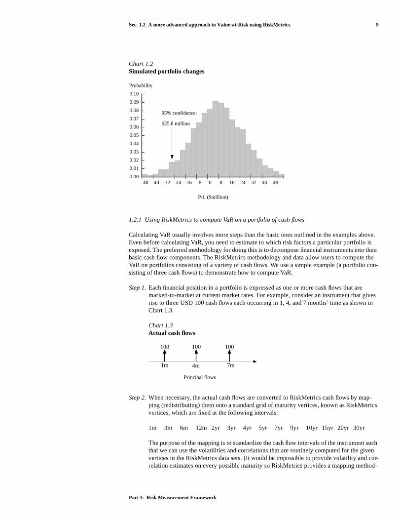
The histogram in Chart 1.2 presents future changes in value of the portfolio. VaR reduces risk to just one number, i.e., a loss associated with a given probability. It is often useful for risk managers to focus on the total distribution of potential gains and losses and we will discuss why this is so later in this document. (See Section 6.3).

3

Where e is approximately 2.27183

4

This number is computed from

V0

V1 V1 V0er

=

r̂r̂

r r̂<( )

V̂1 V̂1 V0er̂

=

V0 V̂1–

V0 1 e–r̂

r̂e

r̂1 r̂+≈ VaR is approximately equal toV0 r̂ V0 r̂

r̂

V0

µ1 0

σ1 0r̂ 1.65σ1 0– µ1 0+=

σ1 0 µ1 0 0=σ1 0 0.0321= V1 USD 474.2 million=

e1.65σ–

V0

V0 V̂1–



Chart 1.2

Simulated portfolio changes

1.2.1 Using RiskMetrics to compute VaR on a portfolio of cash flows

Calculating VaR usually involves more steps than the basic ones outlined in the examples above. Even before calculating VaR, you need to estimate to which risk factors a particular portfolio is exposed. The preferred methodology for doing this is to decompose financial instruments into their basic cash flow components. The RiskMetrics methodology and data allow users to compute the VaR on portfolios consisting of a variety of cash flows. We use a simple example (a portfolio con-sisting of three cash flows) to demonstrate how to compute VaR.

Step 1.

Each financial position in a portfolio is expressed as one or more cash flows that are marked-to-market at current market rates. For example, consider an instrument that gives rise to three USD 100 cash flows each occurring in 1, 4, and 7 months’ time as shown in Chart 1.3.

Chart 1.3

Actual cash flows

Step 2.

When necessary, the actual cash flows are converted to RiskMetrics cash flows by map-ping (redistributing) them onto a standard grid of maturity vertices, known as RiskMetrics vertices, which are fixed at the following intervals:

1m 3m 6m 12m 2yr 3yr 4yr 5yr 7yr 9yr 10yr 15yr 20yr 30yr

The purpose of the mapping is to standardize the cash flow intervals of the instrument such that we can use the volatilities and correlations that are routinely computed for the given vertices in the RiskMetrics data sets. (It would be impossible to provide volatility and cor-relation estimates on every possible maturity so RiskMetrics provides a mapping method-

-48 -40 -32 -24 -16 -8 0 8 16 24 32 40 480.00

0.01

0.02

0.03

0.04

0.05

0.06

0.07

0.08

0.09

0.10

P/L ($million)

95% confidence:

$25.8 million

Probability

100 100100

1m 4m 7m

Principal flows


RiskMetrics


ology which distributes cash flows to a workable set of standard maturities). The methodology for mapping cash flows is detailed in Chapter 6.

To map the cash flows, we use the RiskMetrics vertices closest to the actual vertices and redistribute the actual cash flows as shown in Chart 1.4.

Chart 1.4

Mapping actual cash flows onto RiskMetrics vertices

The RiskMetrics cash flow map is used to work backwards to calculate the return for each of the actual cash flows from the cash flow at the associated RiskMetrics vertex, or vertices.

For each actual cash flow, an analytical expression is used to express the relative change in value of the actual cash flow in terms of an underlying return on a particular instrument. Continuing with Chart 1.4, we can write the return on the actual 4-month cash flow in terms of the combined returns on the 3-month (60%) and 6-month (40%) RiskMetrics cash flows:

[1.2]

where

Similarly, the return on the 7-month cash flow can be written as

[1.3]

Note that the return on the actual 1-month cash flow is equal to the return on the 1-month instrument.

Step 3.

VaR is calculated at the 5th percentile of the distribution of portfolio return, and for a spec-ified time horizon. In the example above, the distribution of the portfolio return, , is written as:

[1.4]

RiskMetrics cashflows

100

Actual cashflows

100 60 3040 70

100 110 3060

Cashflow mapping

100 100

1m 4m 7m

1m 3m 6m 12m

1m 3m 6m 12m

r4m 0.60r3m 0.40r6m+=

r4m return on the actual 4-month cash flow=

r3m return on the 3-month RiskMetrics cash flow=

r6m return on the 6-month RiskMetrics cash flow=

r7m 0.70r6m 0.30r12m+=

rp

rp 0.33r1m 0.20r3m 0.37r6m 0.10r12m+ + +=



where, for example the portfolio weight 0.33 is the result of 100 divided by the total port-folio value 300.

Now, to compute VaR at the 95th percent confidence level we need the fifth percentile of the portfolio return distribution. Under the assumption that is distributed conditionally normal, the fifth percentile is −1.65 where is the standard deviation of the portfolio return distribution. Applying Eq. [1.1] to a portfolio containing more than two instruments requires using simple matrix algebra. We can thus express this VaR calculation as follows:

[1.5]

where is a vector of VaR estimates per instrument,

,

and R is the correlation matrix

[1.6]

where, for example, is the correlation estimate between 1-month and 3-month returns.

Note that RiskMetrics provides the vector of information

as well as the correlation matrix R. What the user has to provide are the actual port-folio weights.

1.2.2 Measuring the risk of nonlinear positions

When the relationship between position value and market rates is nonlinear, then we cannot esti-mate changes in value by multiplying “estimated changes in rates” by “sensitivity of the position to changing rates;” the latter is not constant (i.e., the definition of a nonlinear position). In our pre-vious examples, we could easily estimate the risk of a fixed income or foreign exchange product by assuming a linear relationship between the value of an instrument and the value of its underly-ing. This is not a reasonable assumption when dealing with nonlinear products such as options.

RiskMetrics offers two methodologies, an analytical approximation and a structured Monte Carlo simulation to compute the VaR of nonlinear positions:

1. The first method approximates the nonlinear relationship via a mathematical expression that relates the return on the position to the return on the underlying rates. This is done by using what is known as a Taylor series expansion.

This approach no longer necessarily assumes that the change in value of the instrument is approximated by its delta alone (the first derivative of the option’s value with respect to the underlying variable) but that a second order term using the option’s gamma (the second derivative of the option’s value with respect to the underlying price) must be introduced to

rpσp σp

VaR V RVT

=

V

V 0.33 1.65σ⋅ 1m( ) 0.20 1.65σ3m⋅( ) 0.37 1.65σ6m⋅( ) 0.10 1.65σ12m⋅( ), , ,[ ]=

R

1 ρ3m 1m, ρ6m 1m, ρ12m 1m,

ρ1m 3m, 1 ρ6m 3m, ρ12m 3m,

ρ1m 6m, ρ3m 6m, 1 ρ12m 6m,

ρ1m 12m, ρ3m 12m, ρ6m 12m, 1

=

ρ1m 3m,

V 1.65σ1m( ) 1.65σ3m( ) 1.65σ6m( ) 1.65σ12m( ), , ,[ ]=


RiskMetrics —Technical DocumentFourth Edition

measure the curvature of changes in value around the current value. In practice, other “greeks” such as vega (volatility), rho (interest rate) and theta (time to maturity) can also be used to improve the accuracy of the approximation. In Section 1.2.2.1, we present two types of analytical methods for computing VaR—the delta and delta-gamma approxima-tion.

2. The second alternative, structured Monte Carlo simulation, involves creating a large num-ber of possible rate scenarios and revaluing the instrument under each of these scenarios. VaR is then defined as the 5th percentile of the distribution of value changes. Due to the required revaluations, this approach is computationally more intensive than the first approach.

The two methods differ not in terms of how market movements are forecast (since both use the RiskMetrics volatility and correlation estimates) but in how the value of portfolios changes as a result of market movements. The analytical approach approximates changes in value, while the structured Monte Carlo fully revalues portfolios under various scenarios.

Let us illustrate these two methods using a practical example. We will consider throughout this section a portfolio comprised of two assets:

Asset 1: a future cash flow stream of DEM 1 million to be received in one year’s time. The cur-rent 1-year DEM rate is 10% so the current market value of the instrument is DEM 909,091.

Asset 2: an at-the-money (ATM) DEM put/USD call option with contract size of DEM 1 million and expiration date one month in the future. The premium of the option is 0.0105 and the spot exchange rate at which the contract was concluded is 1.538 DEM/USD. We assume the implied volatility at which the option is priced is 14%.

The value of this portfolio depends on the USD/DEM exchange rate and the one-year DEM bond price. Technically, the value of the option also changes with USD interest rates and the implied volatility, but we will not consider these effects. Our risk horizon for the example will be five days. We take as the daily volatilities of these two assets and and as the correlation between the two .

Both alternatives will focus on price risk exclusively and therefore ignore the risk associated with volatility (vega), interest rate (rho) and time decay (theta risk).

1.2.2.1 Analytical methodThere are various ways to analytically approximate nonlinear VaR. This section reviews the two alternatives which we discussed previously.

Delta approximationThe standard VaR approach can be used to come up with first order approximations of portfolios that contain options. (This is essentially the same simplification that fixed income traders use when they focus exclusively on the duration of their portfolio). The simplest such approximation is to estimate changes in the option value via a linear model, which is commonly known as the ”delta approximation.” Delta is the first derivative of the option price with respect to the spot exchange rate. The value of δ for the option in this example is −0.4919.

In the analytical method, we must first write down the return on the portfolio whose VaR we are trying to calculate. The return on this portfolio consisting of a cash flow in one year and a put on the DEM/call on the USD is written as follows:

[1.7]

σFX 0.42%= σB 0.08%=ρ 0.17–=

rp =r1y rDEMUSD--------------

δrDEMUSD--------------

+ +



where

Under the assumption that the portfolio return is normally distributed, VaR at the 95% confidence level is given by

[1.8]

Using our volatilities and correlations forecasts for DEM/USD and the 1-year DEM rate (scaled up to the weekly horizon using the square root of time rule), the weekly VaR for the portfolio using the delta equivalent approach can be approximated by:

Market value in USD VaR(1w)1-yr DEM cash flow $591,086 $1,745FX position - FX hedge $300,331 $4,654

Diversified VaR$4,684

Delta-gamma approximationThe delta approximation is reasonably accurate when the exchange rate does not change signifi-cantly, but less so in the more extreme cases. This is because the delta is a linear approximation of a non linear relationship between the value of the exchange rate and the price of the option as shown in Chart 1.5. We may be able to improve this approximation by including the gamma term, which accounts for nonlinear (i.e. squared returns) effects of changes in the spot rate (this attempts to replicate the convex option price to FX rate relationship as shown in Chart 1.5). The expression for the portfolio return is now

[1.9]

where

In this example, = DEM/USD 15.14.

Now, the gamma term (the fourth term in Eq. [1.9]) introduces skewness into the distribution of (i.e., the distribution is no longer symmetrical around its mean). Therefore, since this violates

one of the assumptions of normality (symmetry) we can no longer calculate the 95th percentile VaR as 1.65 times the standard deviation of . Instead we must find the appropriate multiple (the counterpart to −1.65) that incorporates the skewness effect. We compute the 5th percentile of ’s distribution (Eq. [1.9]) by computing its first four moments, i.e., ’s mean, variance, skewness and kurtosis. We then find distribution whose first four moments match those of ’s. (See Section 6.3 for details.)

r1 p the price return on the 1-year German interest rates=

rDEMUSD--------------

the return on the DEM/USD exchange rate=

δ the delta of the option=

VaR = 1.65 σ1y2

1 δ+( ) 2σDEMUSD--------------

22 1 δ+( ) ρ

1yDEMUSD--------------,

σ1yσDEMUSD--------------

+ +

rp =r1y rDEMUSD--------------

δrDEMUSD--------------

0.5 Γ PDEMUSD--------------

rDEMUSD--------------

2

⋅+ + +

PDEMUSD--------------

the value of the DEM/USD exchange rate when the VaR forecast is made=

Γ the gamma of the option.=

Γ

rP

rprp

rprp



Applying this methodology to this approach we find the VaR for this portfolio to be USD 3,708. Note that in this example, incorporating gamma reduces VaR relative to the delta only approxima-tion (from USD 5006 to USD 3708).

Chart 1.5Value of put option on USD/DEMstrike = 0.65 USD/DEM. Value in USD/DEM.

1.2.2.2 Structured Monte-Carlo SimulationGiven the limitations of analytical VaR for portfolios whose P/L distributions may not be symmet-rical let alone normally distributed, another possible route is to use a model which instead of esti-mating changes in value by the product of a rate change (σ) and a sensitivity (δ, Γ), focuses on revaluing positions at changed rate levels. This approach is based on a full valuation precept where all instruments are marked to market under a large number of scenarios driven by the volatility and correlation estimates.

The Monte Carlo methodology consists of three major steps:

1. Scenario generation —Using the volatility and correlation estimates for the underlying assets in our portfolio, we produce a large number of future price scenarios in accordance with the lognormal models described previously. The methodology for generating scenarios from volatility and correlation estimates is described in Appendix E.

2. Portfolio valuation — For each scenario, we compute a portfolio value.

3. Summary — We report the results of the simulation, either as a portfolio distribution or as a particular risk measure.

Using our volatility and correlation estimates, we can apply our simulation technique to our exam-ple portfolio. We can generate a large number of scenarios (1000 in this example case) of DEM 1-year and DEM/USD exchange rates at the 1-week horizon. Chart 1.6 shows the actual distribu-tions for both instruments as well as the scattergram indicating the degree of correlation (−0.17) between the two rate series.

0.60 0.61 0.62 0.63 0.64 0.65 0.66 0.67 0.68 0.69 0.70-0.02

-0.01

0

0.01

0.02

0.03

0.04

0.05

0.06

USD/DEM exchange rate

Full valuation

Delta

Delta + gamma

Option value



Chart 1.6Histogram and scattergram of rate distributions2-yr DEM rate and DEM/USD rate

With the set of interest and foreign exchange rates obtained under simulation, we can revalue both of the instruments in our portfolio. Their respective payouts are shown in Chart 1.7.

Chart 1.7Valuation of instruments in sample portfolioValue of the cash flow stream Value of the FX option

The final task is to analyze the distribution of values and select the VaR using the appropriate per-centile. Chart 1.8 shows the value of the components of the portfolio at the end of the horizon period.

9.3% 9.5% 9.7% 10.0%10.2%10.4%10.6%0

20

40

60

80

100

120

1.49 1.50 1.52 1.53 1.55 1.56 1.580

20

40

60

80

100

120

J

J

J

J

J

J

JJ

J

J

J

J

J

J

J

J

JJ

JJJ

J

J

J

J

J

JJ

J

J

J J

J

JJ J

J

J

J

J

J

J

J

J

J

J

JJ

J J

J

J

J

J

J

JJ

J

J

JJ JJ

J

J

J

J

J

JJ

J

J

JJ

J

J

J

JJ

J

J

J

J

J

J

JJJ

J

J

J

J J

JJ

J

J

J

J

J

J

J

J

J

JJ J

J

J

J

J

J

J

J

J

JJ

J

J

J

J

J

J

J J

J

J J

J

J

J

J

J

J

JJJ

J

J

J J

J

J

J

J

J J

J

J

J

JJ

J

J

J

JJ

J

J

J

J

J

J

J

J

J

J

J

J

J

JJ

J

J

J

J J

J

J

J

JJ

J

J

J

J

J

J

J

J

J

J

J

J J

J

J

J

J

J

J

J

J

J J

J

J

J

J

J

J

J

J

J

J

J

J

J

JJ

JJ

J

JJ

J

J

J

J

J

J

J

JJ

J

J

J

J

J

J

JJ

J

J

J

J

J

J

J

J

J

J

JJ

J

JJ

JJ

J

J

J

J

JJ

J

J

JJ

J

J

J

J

J

J

J

J

J

J

J

J

J

J

J

J

J

J

JJ

J

J

J

JJ

JJ

J J

JJ

J

J

J

JJ

JJ J

J

J

JJJ

J

J JJ

J

J

J J

J

J

J

J

J

J

J

J

J

J

J

J

J

J

J

J

J

JJ

J

J

J

J

J

J

J

JJJ

J

J

J

J

J

J

J

J

JJ

J

J

J

JJJ

J

J

J

J

JJ

JJ

J

J

J

J

J

J

J

J

J

J

J

J

J

J J

J

J

J

J

J

J

J

J

J

J

J

J

J

J

J

J

JJ

J

J

J

J

J

J

J

J

J

J

JJ

J

J

J

J

J

J

J

J

J

J

J

J

J

J

JJ

J

J

J

J

J

J

JJ

J

J

J

J

J

J

J

J

J

J

J

J

J

J

J

J

J

J

J

J

J

J

J

J

J

J JJ

J

JJ

J

J

J

J

J

J

J

J

J

J

J

J

J

J

J

J

J

JJ

J

JJ

J

JJ

JJ

J

J

JJ

JJ

J

J

J

J

J J

J

JJ

J

J

J

J

J

J

J

J

J

J

J

J

J

J

J

J

J

J

J

J

J

J

J

J

J

J

J

J

J

J

J

J

J

J

J

J

JJ

J

JJ

J

J J

J

J

J

J

J

JJ

JJ

J

J

J

J

J

J

J

J

JJ

J

J

J

J

J

J

J

J

J

J

J

J

J

JJ

J

J

JJ

J

J

J

J

J

J

J

J

J

J

J

J

J

J

J

J

J

J

J

J

J

J

J

J

J

J J

J

J

J

J

J

JJ

JJ

J J

J

J

J

J

J

J

J

J

J

J

J

JJ

J

J

J

J

J

J

J

J

JJ

J

J

J

J

J

J

J

J

J

J

J

J

J

J

J

J

J

J

J

J

J

J

J

J

J

J

J

J

J

J

J

J

J

J

J

J

J

J

J

J

J

J

J

J

J

J

J

J

J

J

J J

J

J

J

J

J

J

J

J

J

J

J

J

J

J

JJ

J

J

JJ

J

J

J

J

J

J

J

J J

J

J

J

J

J

J

J

J

J

J

J

J

J

J

JJ

JJ

J

J J

J

J

J

J

J

J

J

JJJ

J

J

J

J

J

J

J

J

J

J

J

J

J

J

J

JJ

J

J

J

JJ

J

J

J

J

J

J

JJJ

J

J

J

J

J

J

J

J

J

J

J

J

J

JJ

J

J

J

J

J

JJ

J

J

J

J

J

J

J

JJ

J

JJ

J

J

J

J

J

J

JJ

J

J

J

J

J

J

J

J

J

JJ

J

J

J J

J

J

J

J J

J

J

J

J JJ

J

J

J

J

J

J

J

J

J

J

J

J

J

J

J

J

J

J

J

J

J

J

J

J

J

JJ

J

J

J

JJ

J

J

J

J

J JJ

J

J

J

JJ

J

J

J

J

J

J

JJ

J

J

J

J

J

J

J

J

JJ

J

J J

J

JJ

J

J

J

J

J

J

J

J

J

J

J

J

JJJ

J

J

J

J

J

J

J

J

JJ

J

JJ

J

J

J

J

J

JJ

JJ

J

J

J

J

J

J

J

J

JJ

J

J

JJ

JJ

J

J

J

J

J

J

JJ

J

Frequency Frequency

Yields P/L

9.30 9.55 9.80 10.05 10.30 10.55585.0

587.5

590.0

592.5

595.0

Option value - USD thousands

Yield

0

5

10

15

20

25

1.48 1.5 1.52 1.54 1.56 1.58 1.6

DEM/USD

Cash flow value - USD thousands



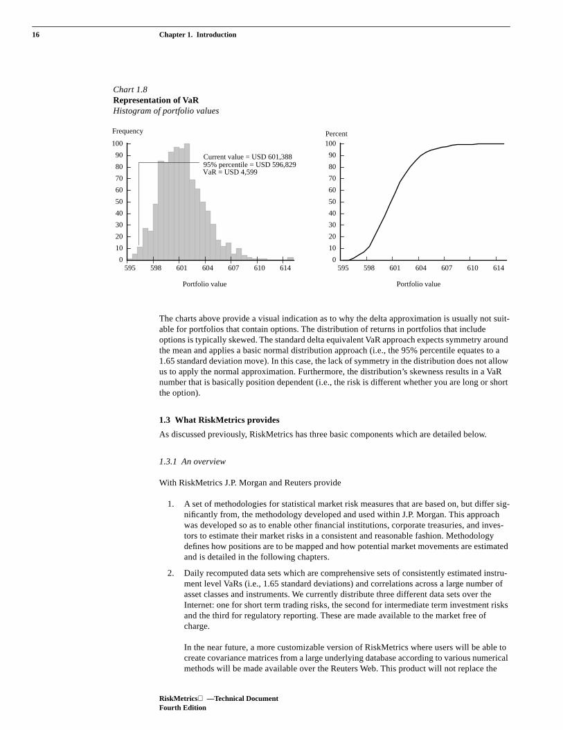
Chart 1.8Representation of VaRHistogram of portfolio values

The charts above provide a visual indication as to why the delta approximation is usually not suit-able for portfolios that contain options. The distribution of returns in portfolios that include options is typically skewed. The standard delta equivalent VaR approach expects symmetry around the mean and applies a basic normal distribution approach (i.e., the 95% percentile equates to a 1.65 standard deviation move). In this case, the lack of symmetry in the distribution does not allow us to apply the normal approximation. Furthermore, the distribution’s skewness results in a VaR number that is basically position dependent (i.e., the risk is different whether you are long or short the option).

1.3 What RiskMetrics provides

As discussed previously, RiskMetrics has three basic components which are detailed below.

1.3.1 An overview

With RiskMetrics J.P. Morgan and Reuters provide

1. A set of methodologies for statistical market risk measures that are based on, but differ sig-nificantly from, the methodology developed and used within J.P. Morgan. This approach was developed so as to enable other financial institutions, corporate treasuries, and inves-tors to estimate their market risks in a consistent and reasonable fashion. Methodology defines how positions are to be mapped and how potential market movements are estimated and is detailed in the following chapters.

2. Daily recomputed data sets which are comprehensive sets of consistently estimated instru-ment level VaRs (i.e., 1.65 standard deviations) and correlations across a large number of asset classes and instruments. We currently distribute three different data sets over the Internet: one for short term trading risks, the second for intermediate term investment risks and the third for regulatory reporting. These are made available to the market free of charge.

In the near future, a more customizable version of RiskMetrics where users will be able to create covariance matrices from a large underlying database according to various numerical methods will be made available over the Reuters Web. This product will not replace the

595 598 601 604 607 610 6140

10

20

30

40

50

60

70

80

90

100

595 598 601 604 607 610 6140

10

20

30

40

50

60

70

80

90

100

Frequency Percent

Current value = USD 601,38895% percentile = USD 596,829VaR = USD 4,599

Portfolio value Portfolio value

Sec. 1.3 What RiskMetrics provides 17


data sets available over the Internet but will provide subscribers to the Reuters services with a more flexible tool.

The four basic classes of instruments that RiskMetrics methodology and data sets cover are represented as follows:

• Fixed income instruments are represented by combinations of amounts of cash flows in a given currency at specified dates in the future. RiskMetrics applies a fixed number of dates (14 vertices) and two types of credit standings: government and non-govern-ment. The data sets associated with fixed income are zero coupon instrument VaR sta-tistics, i.e., 1.65σ, and correlations for both government and swap yield curves.

• Foreign exchange transactions are represented by an amount and two currencies. RiskMetrics allows for 30 different currency pairs (as measured against the USD).

• Equity instruments are represented by an amount and currency of an equity basket index in any of 30 different countries. Currently, RiskMetrics does not consider the individual characteristics of a company stock but only the weighted basket of compa-nies as represented by the local index.

• Commodities positions are represented by amounts of selected standardized commod-ity futures contracts traded on commodity exchanges

3. Software provided by J.P. Morgan, Reuters and third party firms that use the RiskMetrics methodology and data documented herein.

Chart 1.9Components of RiskMetrics

Since the RiskMetrics methodology and the data sets are in the public domain and freely available, anyone is free to implement systems utilizing these components of RiskMetrics. Third parties have developed risk management systems for a wide range of clients using different methodologies. The following paragraphs provide a taxonomy comparing the different approaches.

Blotter (Inventory)Posting

Transaction

Mapping Position EvaluationRisk

/Return Measures

RiskMetrics™ methodology

System implementations

RiskMetrics™ Volatility & correlation

estimates

ValuationProfits &

Losses

Risk Projection

Estimated Risks



1.3.2 Detailed specification

The section below provides a brief overview of how the RiskMetrics datasets are produced and how the parameters we provide can be used in a VaR calculation.

1.3.2.1 Production of volatility and correlation data setsRiskMetrics provides the following sets of volatility and corresponding correlation data files. One set is for use in estimating VaR with a forecast horizon of one day. The other set is optimized for a VaR forecast horizon of one month. The third set is based on the quantitative criteria set by the Bank for International Settlements on the use of VaR models to estimate the capital required to cover market risks. The process by which these data files are constructed are as follows:

1. Financial prices are recorded from global data sources. (In 1997, RiskMetrics will switch to using Reuters data exclusively). For certain fixed income instruments we construct zero rates. See Chapter 9 for data sources and RiskMetrics building blocks.

2. Fill in missing prices by using the Expectation Maximization algorithm (detailed in Section 8.2). Prices can be missing for a variety of reasons, from technical failures to holi-day schedules.

3. Compute daily price returns on all 480 time series (Section 4.1).

4. Compute standard deviations and correlations of financial price returns for a 1-day VaR forecast horizon. This is done by constructing exponentially weighted forecasts. (See Section 5.2). Production of the daily statistics also involves setting the sample daily mean to zero. (See Section 5.3). If data is recorded at different times (Step 1), users may require an adjustment algorithm applied to the correlation estimates. Such an algorithm is explained in Section 8.5. Also, users who need to rebase the datasets to account for a base currency other than the USD should see Section 8.4.

5. Compute standard deviations and correlations of financial price returns for 1-month VaR forecast horizon. This is done by constructing exponentially weighted forecasts (Section 5.3). Production of the monthly statistics also involves setting the sample daily mean to zero.

1.3.2.2 RiskMetrics VaR calculation1. The first step in the VaR calculation is for the user to define three parameters:

(1) VaR forecast horizon—the time over which VaR is calculated, (2) confidence level—the probability that the realized change in portfolio will be less than the VaR prediction, and (3) the base currency.

2. For a given portfolio, once the cash flows have been identified and marked-to-market (Section 6.1) they need to be mapped to the RiskMetrics vertices (Section 6.2).

3. Having mapped all the positions, a decision must be made as to how to compute VaR. If the user is willing to assume that the portfolio return is approximately conditionally normal, then download the appropriate data files (instrument level VaRs and correlations) and com-pute VaR using the standard RiskMetrics approach (Section 6.3).

4. If the user’s portfolio is subject to nonlinear risk to the extent that the assumption of condi-tional normality is no longer valid, then the user can choose between two methodologies—delta-gamma and structured Monte Carlo. The former is an approximation of the latter. See Section 6.3 for a description of delta-gamma and Chapter 7for an explanation of structured Monte Carlo.

19


Chapter 2. Historical perspective of VaR

2.1 From ALM to VaR 222.2 VaR in the framework of modern financial management 24

2.2.1 Valuation 252.2.2 Risk estimation 25

2.3 Alternative approaches to risk estimation 262.3.1 Estimating changes in value 262.3.2 Estimating market movements 27

20

RiskMetrics


21


Chapter 2. Historical perspective of VaR


[email protected]

Measuring the risks associated with being a participant in the financial markets has become the focus of intense study by banks, corporations, investment managers and regulators. Certain risks such as counterparty default have always figured at the top of most banks’ concerns. Others such as market risk (the potential loss associated with market behavior) have only gotten into the lime-light over the past few years. Why has the interest in market risk measurement and monitoring arisen? The answer lies in the significant changes that the financial markets have undergone over the last two decades.

1. Securitization: Across markets, traded securities have replaced many illiquid instruments, e.g., loans and mortgages have been securitized to permit disintermediation and trading. Global securities markets have expanded and both exchange traded and over-the-counter derivatives have become major components of the markets.

These developments, along with technological breakthroughs in data processing, have gone hand in hand with changes in management practices—a movement away from management based on accrual accounting toward risk management based on marking-to-market of posi-tions. Increased liquidity and pricing availability along with a new focus on trading led to the implementation of frequent revaluation of positions, the mark-to-market concept.

As investments became more liquid, the potential for frequent and accurate reporting of investment gains and losses has led an increasing number of firms to manage daily earnings from a mark-to-market perspective. The switch from accrual accounting to mark-to-market often results in higher swings in reported returns, therefore increasing the need for manag-ers to focus on the volatility of the underlying markets. The markets have not suddenly become more volatile, but the focus on risks through mark-to-market has highlighted the potential volatility of earnings.

Given the move to frequently revalue positions, managers have become more concerned with estimating the potential effect of changes in market conditions on the value of their positions.

2. Performance: Significant efforts have been made to develop methods and systems to mea-sure financial performance. Indices for foreign exchange, fixed income securities, commod-ities, and equities have become commonplace and are used extensively to monitor returns within and/or across asset classes as well as to allocate funds.

The somewhat exclusive focus on returns, however, has led to incomplete performance analysis. Return measurement gives no indication of the cost in terms of risk (volatility of returns). Higher returns can only be obtained at the expense of higher risks. While this trade-off is well known, the risk measurement component of the analysis has not received broad attention.

Investors and trading managers are searching for common standards to measure market risks and to estimate better the risk/return profile of individual assets or asset classes. Not-withstanding the external constraints from the regulatory agencies, the management of financial firms have also been searching for ways to measure market risks, given the poten-tially damaging effect of miscalculated risks on company earnings. As a result, banks, investment firms, and corporations are now in the process of integrating measures of mar-ket risk into their management philosophy. They are designing and implementing market risk monitoring systems that can provide management with timely information on positions and the estimated loss potential of each position.

Over the last few years, there have been significant developments in conceptualizing a common framework for measuring market risk. The industry has produced a wide variety of indices to mea-sure return, but little has been done to standardize the measure of risk. Over the last 15 years many market participants, academics, and regulatory bodies have developed concepts for measuring

22 Chapter 2. Historical perspective of VaR

RiskMetrics


market risks. Over the last five years, two approaches have evolved as a means to measure market risk. The first approach, which we refer to as the statistical approach, involves forecasting a portfo-lio’s return distribution using probability and statistical models. The second approach is referred to as scenario analysis. This methodology simply revalues a portfolio under different values of mar-ket rates and prices. Note that in stress scenario analysis does not necessarily require the use of a probability or statistical model. Instead, the future rates and prices that are used in the revaluation can be arbitrarily chosen. Risk managers should use both approaches—the statistical approach to monitor risks continuously in all risk-taking units and the scenario approach on a case-by-case basis to estimate risks in unique circumstances.

This document explains, in detail, the statistical approach—RiskMetrics—to measure market risk.

This chapter is organized as follows:

• Section 2.1 reviews how VaR was developed to support the risk management needs of trading activities as opposed to investment books. Though the distinction to date has been an account-ing one not an economic one, VaR concepts are now being used across the board.

• Section 2.2 looks at the basic steps of the risk monitoring process.

• Section 2.3 reviews the alternative VaR models currently being used and how RiskMetrics provides end-users with the basic building blocks to test different approaches.

2.1 From ALM to VaR

A well established method of looking at market risks in the banking industry is to forecast earn-ings under predetermined price/rate market conditions (or scenarios). Earnings here are defined as earnings reported in a firm’s Financial Statements using generally accepted accounting principles. For many institutions the bulk of activities are reported on an accrual basis, i.e., transactions are booked at historical costs +/- accruals. Only a limited number of trading items are marked to mar-ket. Because changes in market rates manifest themselves only slowly when earnings are reported on an accrual basis, the simulation of income has to be done over extended periods, i.e., until most of the transactions on the books mature. Chart 2.1 illustrates this conventional Asset/Liability Management approach.

Chart 2.1

Asset liability management

There are two major drawbacks to this methodology:

• It requires projecting market rate developments over extended periods into the future.

Projected income

statement

Intermediate termrate forecasts

Income simulation

Accrual items

Trading items

Inventory of financial

transactions

Sec. 2.1 From ALM to VaR 23


• It supports the illusion that gains and losses occur at the time they show up in the accrual accounts (i.e., when they are realized following accounting principles). What this means is that return is only defined as net interest earnings, a framework which ignores the change in price component of the return function.

Every investor would agree that the total return on a bond position is the sum of the interest earned and the change in the value of the bond over a given time horizon. Traditional ALM, as a result of accounting conventions, ignores the change in value of the instrument since posi-tions are not marked to market. This has often lead crafty ALM managers to create positions which look attractive on paper because of high net interest earnings, but which would not per-form as well if their change in market value were considered.

The market risk in trading positions is usually measured differently and managed separately. Trad-ing positions are marked-to-market and the market value is then subjected to projections of changes in short term in rates and prices. This is much less hazardous as rate forecasts are usually limited to short horizons, i.e., the time it should take to close out or hedge the trading position.

Chart 2.2

Value-at-Risk management in trading

The distinction between accrual items and trading items and their separate treatment for market risk management has led to significant complications—particularly when transactions classified as “trading items” under generally accepted accounting principles are used to hedge transactions classified as “accrual items”. In an effort to overcome this difficulty, many firms – particularly those with relatively large trading books have expanded the market risk approach to also include accrual items, at least for internal risk management reporting. This is done by estimating the fair market value of the accrual items and the changes in their fair value under different short term sce-narios. Thus we are witnessing the evolution of an alternative to the conventional approach of Asset/Liability Management, the Value-at-Risk approach. It started in pure trading operations, but is now gaining increased following in the financial industry.


transactions

Current market rates & prices

“mark to market” Market

values

Value simulation

Projected market value

changes

Short term price forecasts

Accrual items

Trading items


RiskMetrics


Chart 2.3

Comparing ALM to VaR management

The advantages of VaR Management are that it

• Incorporates the mark-to-market approach uniformly.

• Relies on a much shorter horizon forecast of market variables. This improves the risk estimate as short horizon forecasts tend to be more accurate than long horizon forecasts.

Of course, drawbacks exist. One of them is that it may not be trivial to mark certain transactions to market or even understand their behavior under certain rate environments. This is particularly true for instruments such as demand deposits in a retail banking environment for example. Whatever the difficulties, the aim of getting an integrated picture of a firm’s exposure to market risks is worth a number of assumptions, some of which may be reasonable representations of reality. In the case of demand deposits, a recent article by Professor Robert Jarrow outlines how power swaps could be modelled to represent a retail bank’s core deposit base risks (RISK, February 1996).

Some critics also argue that marking-to-market all transactions over short time periods creates too much “earnings” or volatility. Looking at risks in this fashion may be misleading. This is the direc-tion of the industry and its accounting regulators however and it will be up to financial analysts to adapt to the new environment. The volatility of earnings will not just appear out of the blue. The changes in accounting practices will ultimately show economic reality as it really is.

Market risk can be absolute or relative. In its absolute form, what is measured is the loss in the value of a position or a portfolio resulting from changes in market conditions. Absolute market risk is what managers of trading operations measure. Corporates who wish to estimate real poten-tial losses from their treasury operations also focus on absolute market risk. Regulators are inter-ested in absolute market risks in relation to a firm’s capital. When investment performance is measured against an index, the inherent market risk is relative in the sense that it measures the potential underperformance against a benchmark.

2.2 VaR in the framework of modern financial management

As discussed before there are two steps to VaR measurement. First, all positions need to be marked to market (valuation). Second we need to estimate the future variability of the market value. Chart 2.4 illustrates this point.

“mark to market”

Proxy values

Market values

Income simulation

Projected income

statement Risk factors

Projected market value

changes

Intermediate termrate forecasts

Short term price forecasts

Conventional Asset/Liability Management

New “Value at Risk”

Management


Accrual items

Trading items


transactions

Sec. 2.2 VaR in the framework of modern financial management 25


Chart 2.4

Two steps beyond accounting

2.2.1 Valuation

Trading items are valued at their current prices/rates as quoted in liquid secondary markets. To value transactions for which, in the absence of a liquid secondary market, no market value exists, we first map them into equivalent positions, or decompose them into parts for which secondary market prices exist. The most basic such “part” is a single cash flow with a given maturity and cur-rency of the payor. Most transactions can be described as a combination of such cash flows and thus can be valued approximately as the sum of market values of their component cash flows.

Only non-marketable items that contain options cannot be valued in this simple manner. For their valuation we also need expected volatilities and correlations of the prices and rates that affect their value, and we need an options pricing model. Volatilities describe potential movements in rates with a given probability; correlations describe the interdependencies between different rates and prices. Thus, for some valuations, we require volatilities and correlations.

2.2.2 Risk estimation

Here we estimate value changes as a consequence of expected changes in prices and rates. The potential changes in prices are defined by either specific scenarios or a set of volatility and correla-tion estimates. If the value of a position depends on a single rate, then the potential change in value is a function of the rates in the scenarios or volatility of that rate. If the value of a position depends on multiple rates, then the potential change in its value is a function of the combination of rates in each scenario or of each volatility and of each correlation between all pairs of rates.

Generating equivalent positions on an aggregate basis facilitates the simulation. As will be shown later, the simulation can be done algebraically (using statistics and matrix algebra), or exhaustively by computing estimated value changes for many combinations of rate changes.

In the RiskMetrics framework, forecasts of volatilities and correlations play a central role. They are required for valuations in the case of derivatives, the critical inputs for risk estimation.

Market Risks

Total Position

Risk Projection

Mapping

Economic values

MappingAccrual items

Trading items

Accounting

Equivalent Position

Trading items

Valuation


Projected scenarios or estimated volatilities &

correlations

Balance Sheet


RiskMetrics


2.3 Alternative approaches to risk estimation

More than one VaR model is currently being used and most practitioners have selected an approach based on their specific needs, the types of positions they hold, their willingness to trade off accuracy for speed (or vice versa), and other considerations.

The different models used today differ on basically two fronts:

• How the changes in the values of financial instruments are estimated as a result of market movements.

• How the potential market movements are estimated.

What makes the variety of models currently employed is the fact that the choices made on the two fronts mentioned above can be mixed and matched in different ways.

2.3.1 Estimating changes in value

There are basically two approaches to estimating how the value of a portfolio changes as a result of market movements: analytical methods and simulation methods.

2.3.1.1 Analytical methods

One such method is the analytical sensitivity approach based on the following equation:

estimated value change =

f

(position sensitivity, estimated rate/price change)

where the position sensitivity factor establishes the relationship between the value of the instru-ment and of the underlying rate or price, and determines the accuracy of the risk approximation.

In its simplest form, the analytical sensitivity approach looks like this:

estimated value change = position sensitivity

×

estimated rate change

For example, the value change of a fixed income instrument can be estimated by using the instru-ment’s duration. Although this linear approximation simplifies the convex price/yield relationship of a bond, it is extensively used in practice because duration often accounts for the most signifi-cant percentage of the risk profile of a fixed income instrument. Similar simplifications can be made for options where the estimated change in value is approximated by the option’s delta.

The initial versions of RiskMetrics basically used an analytical VaR approach that assumed that market risk could be estimated by using a simple first-order approximation such as the one out-lined above. We have since extended the analytical approach to account for nonlinear relationships between market value and rate changes (e.g., options), which requires accounting for gamma risk in addition to delta risk. The more refined version of the analytical approach looks like this:

estimated value change = (position sensitivity 1

×

estimated rate change) + 1/2 (position sensitivity 2)

×

(estimated rate change)

2

+...

In the case of an option, the first-order position sensitivity is the delta, while the second-order term is the gamma. Higher order effects can also be estimated using an analytical approach, but the math typically gets more complex.

The analytical approach requires that positions be summarized in some fashion so that the esti-mated rate changes can be applied. This process of aggregating positions is called mapping and is described in Chapter 6.

Sec. 2.3 Alternative approaches to risk estimation 27


The advantages of analytical models is that they are computationally efficient and enable users to estimate risk in a timely fashion.

2.3.1.2 Simulation methods

The second set of approaches, typically referred to as Full Valuation models rely on revaluing a portfolio of instruments under different scenarios. How these scenarios are generated varies across models, from basic historical simulation to distributions of returns generated from a set of volatil-ity and correlation estimates such as RiskMetrics. Some models include user-defined scenarios that are based off of major market events and which are aimed at estimating risk in crisis condi-tions. This process is often referred to a stress testing.

Full Valuation models typically provide a richer set of risk measures since users are able to focus on the entire distribution of returns instead of a single VaR number. Their main drawback is the fact that the full valuation of large portfolios under a significant number of scenarios is computa-tionally intensive and takes time. It may not be the preferred approach when the goal is to provide senior management with a timely snapshot of risks across a large organization.

2.3.2 Estimating market movements

The second discriminant between VaR approaches is how market movements are estimated. There is much more variety here and the following list is not an exhaustive list of current practice.

RiskMetrics

RiskMetrics uses historical time series analysis to derive estimates of volatilities and correlations on a large set of financial instruments. It assumes that the distribution of past returns can be mod-elled to provide us with a reasonable forecast of future returns over different horizons.

While RiskMetrics assumes conditional normality of returns, we have refined the estimation pro-cess to incorporate the fact that most markets show kurtosis and leptokurtosis. We will be publish-ing factors to adjust for this effect once the RiskMetrics customizable data engine becomes available on the Reuters Web.

These volatility and correlation estimates can be used as inputs to:

• Analytical VaR models

• Full valuation models. In Appendix E we outline how the RiskMetrics volatility and correla-tion data sets can be used to drive simulations of future returns.

Historical Simulation

The historical simulation approach, which is usually applied under a full valuation model, makes no explicit assumptions about the distribution of asset returns. Under historical simulation, portfo-lios are valued under a number of different historical time windows which are user defined. These lookback periods typically range from 6 months to 2 years.

Once the RiskMetrics customizable data engine becomes available on the ReutersWeb, users will be able to access the underlying historical data needed to perform this type of simulation.

Monte Carlo Simulation

While historical simulation quantifies risk by replicating one specific historical path of market evolution, stochastic simulation approaches attempt to generate many more paths of market returns. These returns are generated using a defined stochastic process (for example, assume that interest rates follow a random walk) and statistical parameters that drive the process (for example, the mean and variance of the random variable).The RiskMetrics data sets can be used as inputs to this process.


RiskMetrics


In addition, the following VaR models add refinements to the results generated by the approaches listed above.

Implied volatilities

Some practitioners will also look to the market to provide them with an indication of future poten-tial return distributions. Implied volatility as extracted from a particular option pricing model is the market’s forecast of future volatility. Implied volatilities are often used in comparison to his-tory to refine the risk analysis.

Implied volatilities are not currently used to drive global VaR models as this would require observ-able options prices on all instruments that compose a portfolio. Unfortunately, the universe of con-sistently observable options prices is not yet large enough; generally only exchange traded options are reliable sources of prices. In particular, the number of implied correlations that can be derived from traded options prices is insignificant compared to the number of correlations required to esti-mate risks in portfolios containing many asset types.

User-defined scenarios

Most risk management models add user-defined rate and price movements to the standard VaR number, if only to test the effect of what could happen if historical patterns do not repeat them-selves. Some scenarios are subjectively chosen while others recreate past crises events. The latter is referred to as stress testing and is an integral part of a well designed risk management process.

Selecting the appropriate measurement method is not, however, straightforward. Judgment in the choice of methodologies will always be important. Cost benefit trade-offs are different for each user, depending on his position in the markets, the number and types of instruments traded, and the technology available. Different choices can be made even at different levels of an organization, depending on the objectives. While trading desks of a bank may require precise risk estimation involving simulation on relatively small portfolios, senior management may opt for an analytical approach that is cost efficient and timely. It is important for senior management to know whether the risk of the institution is $10 million or $50 million. It is irrelevant for them to make the distinc-tion between $10 million and $11 million. Achieving this level of accuracy at the senior manage-ment level is not only irrelevant, but can also be unachievable operationally, or at a cost which is not consistent with shareholder value.

Since its introduction, RiskMetrics has become the umbrella name for a series of VaR methodolo-gies, from the simple analytical estimation based on the precept that all instruments are linear (the so-called delta approximation) to the structured Monte Carlo simulation.

Not all participants with exposure to the financial and commodities markets will have the resources to perform extensive simulations. That is why we have strived in this update of the

RiskMetrics— Technical Document

to refine analytical approximations of risk for non-linear instruments (the delta-gamma approximations). During 1997, the availability of historical rates and prices under the RiskMetrics customizable data engine will make historical simulation an option for users of our products.

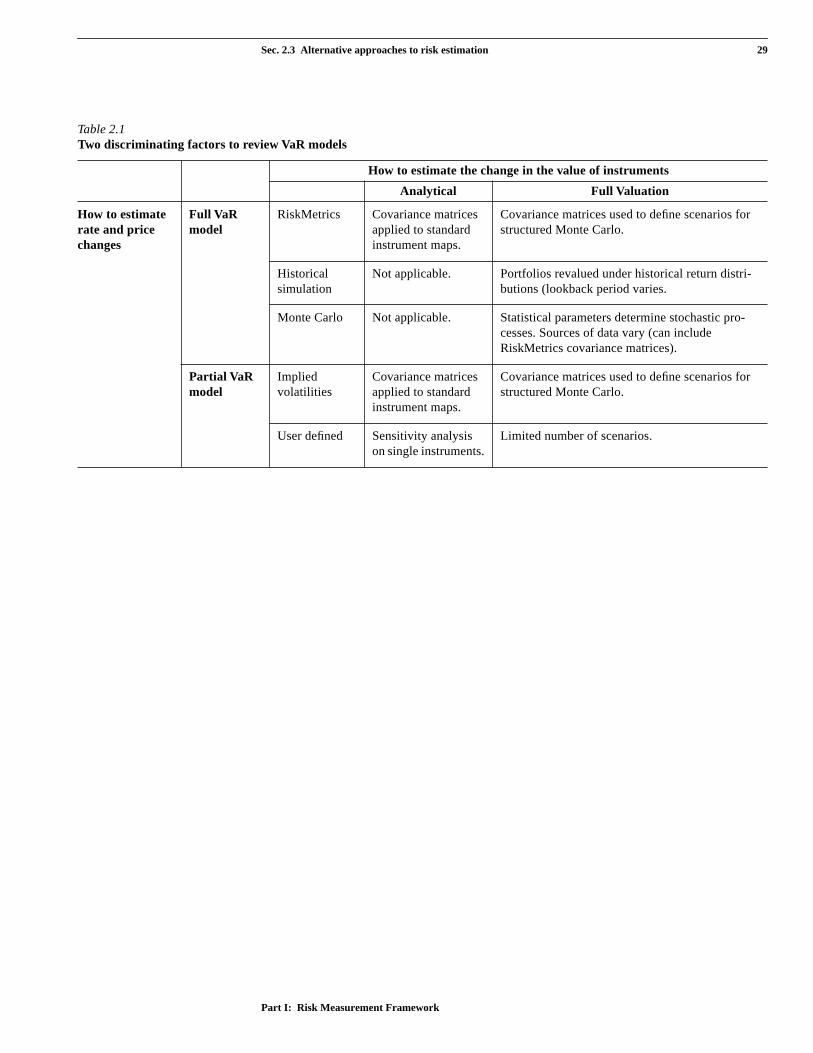
Sec. 2.3 Alternative approaches to risk estimation 29


Table 2.1

Two discriminating factors to review VaR models

How to estimate the change in the value of instruments

Analytical Full Valuation

How to estimate rate and price changes

Full VaR model

RiskMetrics Covariance matrices applied to standard instrument maps.

Covariance matrices used to define scenarios for structured Monte Carlo.

Historical simulation

Not applicable. Portfolios revalued under historical return distri-butions (lookback period varies.

Monte Carlo Not applicable. Statistical parameters determine stochastic pro-cesses. Sources of data vary (can include RiskMetrics covariance matrices).

Partial VaR model

Implied volatilities

Covariance matrices applied to standard instrument maps.

Covariance matrices used to define scenarios for structured Monte Carlo.

User defined Sensitivity analysis on single instruments.

Limited number of scenarios.


RiskMetrics


31


Chapter 3. Applying the risk measures

3.1 Market risk limits 333.2 Calibrating valuation and risk models 343.3 Performance evaluation 343.4 Regulatory reporting, capital requirement 36

3.4.1 Capital Adequacy Directive 363.4.2 Basel Committee Proposal 37

32

RiskMetrics


33


Chapter 3. Applying the risk measures


[email protected]

The measures of market risk outlined in the preceding sections can have a variety of applications. We will highlight just a few:

• To measure and compare market risks.

• To check the valuation/risk models.

• To evaluate the performance of risk takers on a return/risk basis.

• To estimate capital levels required to support risk taking.

3.1 Market risk limits

Position limits have traditionally been expressed in nominal terms, futures equivalents or other denominators unrelated to the amount of risk effectively incurred. The manager of a USD bond portfolio will be told for example that he cannot hold more than 100 million USD worth of U.S. Treasury bonds. In most cases, the measure contains some risk constraint expressed in a particular maturity or duration equivalent (if the 100 million limit is in 2-year equivalents, the manager will not be able to invest 100 million in 30-year bonds). Setting limits in terms of Value-at-Risk has significant advantages: position benchmarks become a function of risk and positions in different markets while products can be compared through this common measure. A common denominator rids the standard limits manuals of a multitude of measures which are different for every asset class. Limits become meaningful for management as they represent a reasonable estimate of how much could be lost.

A further advantage of Value-at-Risk limits comes from the fact that VaR measures incorporate portfolio or risk diversification effects. This leads to hierarchical limit structures in which the risk limit at higher levels can be lower than the sum of risk limits of units reporting to it.

Chart 3.1

Hierarchical VaR limit structure

Setting limits in terms of risk helps business managers to allocate risk to those areas which they feel offer the most potential, or in which their firms’ expertise is greatest. This motivates managers of multiple risk activities to favor risk reducing diversification strategies.

Business AreaVaR-Limit:

$20MM

Business Group AVaR-Limit:

$10MM

Business Group BVaR-Limit:

$12MM

Business Group CVaR-Limit:

$8MM

Unit A1VaR-Limit:

$8MM

Unit A2VaR-Limit:

$7MM

Unit C1VaR-Limit:

$6MM

Unit C2VaR-Limit:

$5MM

Unit C3VaR-Limit:

$3MM

34 Chapter 3. Applying the risk measures

RiskMetrics


3.2 Calibrating valuation and risk models

An effective method to check the validity of the underlying valuation and risk models is to com-pare DEaR estimates with realized daily profits and losses over time. Chart 3.2 illustrates the con-cept. The stars show the daily P&L of a global trading business during the first 7 months of 1993, the two lines show the Daily Earnings at Risk, plus and minus.

Chart 3.2

Ex post validation of risk models: DEaR vs. actual daily P&L

By definition, the cone delimited by the

+/−

DEaR lines should contain 90% of all the stars, because DEaR is defined as the maximum amount of expected profit or losses 90% of the time. If there are substantially more than 10% of the stars outside the DEaR-cone, then the underlying models underestimate the risks. If there are no stars outside the DEaR cone and not even close to the lines, then the underlying models overestimate the risks.

This type of chart is only a reasonable reflection of the risk statistics if the daily profit and losses are derived solely from overnight risk taking and not intraday trading and other activities. Often this is not the case. Then instead of the daily P&L you should plot what is often referred to as the “no-action-P&L”; it describes the hypothetical P&L on the position that would have been incurred if the previous day’s closing position had been kept for the next 24 hours and then revalued. This data is often difficult to collect.

3.3 Performance evaluation

To date, trading and position taking talent have been rewarded to a significant extent on the basis of total returns. Given the high rewards bestowed on outstanding trading talent this may bias the trading professionals towards taking excessive risks.It is often referred to as giving traders a free option on the capital of your firm. The interest of the firm or capital provider may be getting out of line with the interest of the risk taking individual unless the risks are properly measured and returns are adjusted for the amount of risk effectively taken.

✦

✦

✦

✦✦

✦

✦

✦

✦

✦✦✦

✦

✦

✦

✦

✦✦✦✦

✦

✦

✦

✦

✦

✦✦

✦✦

✦

✦

✦✦

✦

✦

✦✦✦

✦

✦✦✦✦✦✦✦

✦✦

✦✦✦✦✦

✦

✦✦✦

✦✦✦✦✦✦

✦✦

✦

✦

✦

✦✦✦

✦

✦

✦✦✦

✦

✦

✦

✦✦✦

✦

✦

✦

✦✦

✦

✦

✦

✦

✦

✦

✦

✦

✦✦

✦

✦

✦

✦

✦

✦

✦

✦

✦

✦✦✦

✦

✦

✦✦

✦

✦✦

✦

✦

✦✦

✦

✦

✦

✦✦

✦

✦

✦

✦

✦

✦

✦✦✦

✦

✦

✦✦

✦

✦✦

✦

✦

✦

-7.5

-5.0

-2.5

0

2.5

5.0

7.5

Jan Feb Mar Apr May Jun Jul

+ DEaR

- DEaR

Sec. 3.3 Performance evaluation 35


To do this correctly one needs a standard measure of risks. Ideally risk taking should be evaluated on the basis of three interlinked measures: revenues, volatility of revenues, and risks. This is illus-trated by Chart 3.3:

Chart 3.3

Performance evaluation triangle

Including estimated (ex ante) and realized (ex post) volatility of profits adds an extra dimension to performance evaluation. The ratio of P&L over risk (risk ratio) and of P&L over volatility (Sharpe ratio) can be combined into what we define as a trader’s efficiency ratio (estimated risk/realized volatility) that measures an individual’s capacity to translate estimated risk into low realized vola-tility of revenues.

Consider an example to illustrate the issue. Assume you have to evaluate Trader #1 relative to Trader #2 and the only information on hand is the history of their respective cumulative trading revenues (i.e., trading profits). This information allows you to compare their profits and volatility of their profits, but says nothing about their risks.

Chart 3.4

Example: comparison of cumulative trading revenues

cumulative revenues

RevenuesVolatility

of revenues

Risks

Risk Ratio

Efficiency Ratio

Sharpe Ratio

-1

0

1

2

3

4

5

6

1992 1993

Trader #1

-1

0

1

2

3

4

5

6

1992 1993

Trader #2


RiskMetrics


With risk information you can compare the traders more effectively. Chart 3.5 shows, for the two traders the risk ratio, sharpe ratio, and efficiency ratio over time.

Chart 3.5

Example: applying the evaluation triangle

Note, you have no information on the type of market these traders operate in or the size of posi-tions they have taken. Nevertheless Chart 3.5 provides interesting comparative information which lead to a richer evaluation.

3.4 Regulatory reporting, capital requirement

Financial institutions such as banks and investment firms will soon have to meet capital require-ments to cover the market risks that they incur as a result of their normal operations. Currently the driving forces developing international standards for market risk based capital requirements are the European Community which issued a binding Capital Adequacy Directive (EC-CAD) and the Basel Committee on Banking Supervision at the Bank for International Settlements (Basel Com-mittee) which has recently come out with revised proposals on the use of banks internal models. (See Appendix F for more information.)

3.4.1 Capital Adequacy Directive

The European Union’s EEC 93/6 directive mandates banks and investment firms to set capital aside to cover market risks. In a nutshell the EC-CAD computes the capital requirement as a sum of capital requirements on positions of different types in different markets. It does not take into account the risk reducing effect of diversification. As a result, the strict application of the current recommendations will lead to financial institutions, particularly the ones which are active interna-tionally in many different markets, to overestimate their market risks and consequently be required to maintain very high capital levels. While there may be some prudential advantages to this, it is

-0.6

0

0.6

-0.2

0

0.2

0.4

0

1

2

1992 1993

Trader #2

-0.6

0

0.6SharpeRatio

RiskRatio

-0.2

0

0.2

0.4

0

1

2

1992 1993

EfficiencyRatio

Trader #1

P&Lvol(P&L)

P&LDEaR

DEaRvol(P&L)

Sec. 3.4 Regulatory reporting, capital requirement 37


not an efficient allocation of financial resources and could lead certain activities to be moved out-side the jurisdiction of the financial regulatory authorities.

3.4.2 Basel Committee Proposal

In January 1996, the Basel Committee on Banking Supervision of the BIS issued a revised consul-tative proposal on an “Internal Model-Based Approach to Market Risk Capital Requirements” that represents a big step forward in recognizing the new quantitative risk estimation techniques used by the banking industry. These proposals recognize that current practice among many financial institutions has superseded the original guidelines in terms of sophistication, and that banks should be given the flexibility to use more advanced methodologies. This so-called “internal models” approach addresses a number of issues that were raised when banks commented on the original proposal dated April 1993.

Table 3.1 compares the methodologies for estimating market risks as recently proposed by the Basel Committee with the RiskMetrics methodology covered in this document. This comparison focuses exclusively on the so-called quantitative factors that the BIS guidelines will require banks to use. It does not address the qualitative ones related to the risk management process and which are beyond the scope of this document.

While the methodologies outlined in the BIS proposals have come a long way in overcoming important objections to the first set of proposals, there are still a number of issues that will be debated further. In order to facilitate the discussion between regulators and regulated, we have published since mid-1995 in parallel with the existing volatility and correlation data sets, a RiskMetrics Regulatory Data Set. The distribution of this regulatory data set is not an endorsement of the Basel committee proposals and the following paragraphs which explain how the data set can be used do not constitute J.P. Morgan’s official position on the content and scope of the Basel com-mittee proposal.

Consistent with the other RiskMetrics data sets, the Regulatory Data Set contains volatility esti-mates for a 1-day holding period. Given that the BIS rules require market risk estimates to be cal-culated over a 10-day holding period and a 99% confidence interval (i.e., 2.33 standard deviations), users will need to rescale the 1-day volatility (see Eq. [3.1]). The Basel proposals allow for this adjustment of data (they actually refer to scaling up VaR estimates but exclude this practice in the case of options since it only works for instruments’ whose pricing formulae are lin-ear). Scaling up volatility estimates is perfectly legitimate, assuming no autocorrelation in the data. Scaling up Value-at-Risk does not work for options, though using scaled up volatilities to estimate the market risks of options with adequate pricing algorithms poses no problem.

As in the other data sets, volatilities and correlations are measured as daily log changes in rates and prices. However, contrary to the exponential weighting schemes used for the other data sets, estimates in the Regulatory Data Set are based on simple moving averages of 1 year of historical data, sampled daily.

To make it comparable to the standard data sets, the RiskMetrics Regulatory Data Set is based on 95% confidence. Including the adjustment for the holding period, users downloading the data sets will need to rescale the volatility estimates according to the following equation, in order to meet the requirements set forth in the Basel proposals (this adjustment assumes a normal distribution. More refined methods incorporating the characteristics of fat tailed distributions are outlined in the statistics section of this document):

[3.1] VBasel

2.331.65---------- V⋅

RiskMetrics RD10⋅=

4.45 VRiskMetrics RD⋅=


RiskMetrics


where

Correlations across asset classes (i.e., foreign exchange to government bonds for example) are supplied in the RiskMetrics Regulatory Data Set, despite the fact that actual use of empirical cor-relations in the VaR estimates is subject to regulatory approval. The BIS has stated that the use of correlations across asset classes would be based on whether the supervisory authority was satisfied with the integrity of the estimation methodology.

VRiskMetrics RD volatilities provided in RiskMetrics Regulatory Dataset=

VBasel volatilities suggested by Basel Committee for use in internal models=

Sec. 3.4 Regulatory reporting, capital requirement 39


Table 3.1

Comparing the Basel Committee proposal with RiskMetrics

Issue Basel Committee proposal RiskMetrics

Mapping:

how positions are described in summary form

• Fixed Income: at least 6 time buckets, differentiate government yield curves and spread curves.

• Equities: country indices, individual stocks on basisof beta equivalent.

• Commodities: to be included, not specified how.

• Fixed Income: data for 7–10 buckets of government yield curves in 16 markets, 4 buckets money market rates in 27 markets, 4–6 buckets in swap rates in 18 markets.

• Equities: country indices in 27 markets, individual stocks on beta (correction for non-systematic risk).

• Commodities: 80 volatility series in 11 commodities (spot and term).

Volatility

: how statistics of future price movement are estimated

• Volatility expressed in standard deviation of normal distribution proxy for daily historical observations year or more back. Equal weights or alternative weighting scheme provided effective observation period is at least one year.

• Estimate updated at least quarterly.

• Volatility expressed in standard deviation of normal distribution proxy for exponentially weighted daily historical observations with decay factors of .94 (for trading, 74 day cutoff 1%) and .97 (for investing, 151 day cutoff at 1%).

• Special Regulatory Data Set, incorporating Basel Committee 1-year moving average assumption.

• Estimates updated daily.

Adversity:

size of adverse move in terms of normal distribution

• Minimum adverse move expected to happen with probability of 1% (2.32 standard deviations) over 10 business days. Permission to use daily statistics scaled up with square root of 10 (3.1). Equivalent to 7.3 daily standard deviations.

• For trading: minimum adverse move expected to happen with probability of 5% (1.65 standard deviation) over 1 business day.

• For investment: minimum adverse move expected to happen with probability of 5% (1.65 standard deviation) over 25 business days.

Options:

treatment of time value and non-linearity

• Risk estimate must consider effect of non-linear price movement (gamma-effect).

• Risk estimate must include effect of changes in implied volatilities (vega-effect).

• Non-linear price movement can be estimated analytically (delta-gamma) or under simulation approach. Simulation scenarios to be generated from estimated volatilities and correlations.

• Estimates of volatilities of implied volatilities currently not pro-vided, thus limited coverage of options risk.

Correlation:

how risks are aggregated • Portfolio effect can be considered within asset classes

(Fixed Income, Equity, Commodity, FX). Use of cor-relations across asset classes subject to regulatory approval.

• Correlations estimated with equally weighted daily data for more than one year.

• Full portfolio effect considered across all possible parameter combinations.

• Correlations estimated using exponentially weighted daily histor-ical observations with decay factors of 0.94 (for trading, 74 day cutoff 1%) and 0.97 (for investing, 151 day cutoff at 1%).

Residuals:

treatment of instrument specific risks

• Instrument specific risks not covered by standard maps should be estimated.

• Capital requirements at least equal to 50% of charge calculated under standard methodology.

• Does not deal with specific risks not covered in standard maps.


RiskMetrics


Documents

J.P.Morgan/Reuters RiskMetrics TM —Technical Document …pascal.iseg.utl.pt/~aafonso/eif/rm/TD4ePt_1.pdf · iv Preface to the fourth edition RiskMetrics —Technical Document Fourth