Journal SCIENCE CLDIRECT 'Microbiological … C. Yang et al. /Journal of Microbiological Methods 65 (2006) 49-62 The computational analyses were performed on two different sets of

Available online at www.sciencedirect.comJournal'MicrobiologicalMethods

SCIENCE CLDIRECT .

Journal of Microbiological Methods 65 (2006) 49-62ELSEVIERwww.elsevier.com/locate/jmicmeth

An ecoinformatics tool for microbial community studies:Supervised classification of Amplicon LengthHeterogeneity (ALH) profiles of 16S rRNA

Chengyong Yang a, DeEtta Mills b, Kalai Mathee b, Yong Wang a, Krish Jayachandran C,

Masoumeh Sikaroodi d, Patrick Gillevet d, Jim Entry e, Giri Narasimhan a'*

aBioinformatics Research Group (BioRG), School of Computer Science, Florida International University, Miami, Florida, 33199, USAbDepartment of Biological Sciences, Florida International University, Miami, Florida, USA

'Department of Environmental Sciences, Florida International University, Miami, Florida, USAdMicrobial and Environmental Biocomplexity, Department of Environmental Sciences and Policy, George Mason University,

Manassas, Virginia, USA'USDA Agricultural Research Service, Northwest Irrigation and Soils Research Laboratory, Kimberly, Idaho, USA

Received 18 January 2005; received in revised form 22 April 2005; accepted 24 June 2005Available online 27 July 2005

Abstract

Support vector machines (SVM) and K-nearest neighbors (KNN) are two computational machine learning tools thatperform supervised classification. This paper presents a novel application of such supervised analytical tools for microbialcommunity profiling and to distinguish patterning among ecosystems. Amplicon length heterogeneity (ALH) profiles fromseveral hypervariable regions of 16S rRNA gene of eubacterial communities from Idaho agricultural soil samples and fromChesapeake Bay marsh sediments were separately analyzed. The profiles from all available hypervariable regions wereconcatenated to obtain a combined profile, which was then provided to the SVM and KNN classifiers. Each profile waslabeled with information about the location or time of its sampling. We hypothesized that after a learning phase usingfeature vectors from labeled ALH profiles, both these classifiers would have the capacity to predict the labels of previouslyunseen samples. The resulting classifiers were able to predict the labels of the Idaho soil samples with high accuracy. Theclassifiers were less accurate for the classification of the Chesapeake Bay sediments suggesting greater similarity within theBay's microbial community patterns in the sampled sites. The profiles obtained from the VI +V2 region were moreinformative than that obtained from any other single region. However, combining them with profiles from the V1 region(with or without the profiles from the V3 region) resulted in the most accurate classification of the samples. The addition

* Corresponding author. Tel.: +1 305 348 3748; fax: +1 305 348 3549.E-mail address: [email protected] (G. Narasimhan).

0167-7012/$ - see front matter © 2005 Elsevier B.V. All rights reserved.doi:10.1016/j.mimet.2005.06.012

50 C. Yang et al. /Journal of Microbiological Methods 65 (2006) 49-62

of profiles from the V9 region appeared to confound the classifiers. Our results show that SVM and KNN classifiers canbe effectively applied to distinguish between eubacterial community patterns from different ecosystems based only on theirALH profiles.CO 2005 Elsevier B.V. All rights reserved.

Keywords: Ecoinformatics; Supervised classification; Machine learning; Amplicon length heterogeneity; Ecosystem community patterns;Support vector machines

1. Introduction

Microbial communities that occur in both naturaland man-made environments can be complex, consist-ing of a large number of bacterial, archaeal, andfungal species. Thus, it is impractical to use culture-based microbiological methods for species identifica-tion. Understanding and analyzing at a whole-com-munity level enables fast and efficient ways to providea glimpse into the patterned diversity of such com-munities (Dunbar et al., 2002; Hill et al., 2002).Molecular methods based on amplification of DNAusing polymerase chain reaction (PCR), cloning andsequencing of highly conserved prokaryotic targetgenes have played a central role in determining theextent of diversity. The predominant choice for atarget gene has been the 16S small subunit ribosomalRNA (rRNA) (Olsen et al., 1986; Pace et al., 1986),resulting in the accumulation of extensive sequenceinformation (e.g., the Ribosome Database Project(Maidak et al., 1999)).

Ribosomal RNA is essential for cellular growth,function, and survival of all organisms. Consequent-ly, ribosomes have highly conserved functionaldomains that share high sequence identity. Theseconserved regions are interspersed with hypervariablesequence regions that are due to base substitutions, orinsertions or deletions of short segments of nucleo-tides. These variations are phylogenetically relevantas they are related to the genetic makeup of eachspecies (Ludwig and Schleifer, 1994). The naturalvariations and composition of 16S rRNA have beenexploited in molecular assays such as terminal re-striction fragment length polymorphism (TRFLP)and amplicon length heterogeneity (ALH). Theseassays depend on the amplification of the variableregions of the 16S rRNA (or any other appropriategene) using sets of primers that are designed basedon the highly conserved regions. The portion of the

DNA sequence amplified by a pair of primers isreferred to as an amplicon. Given a sample consistingof a community of microbes, PCR amplificationusing a pair of primers will yield a profile of ampli-con lengths associated with the microorganisms inthe sample, where the height (intensity) of the peak isproportional to the abundance of the amplicons asso-ciated with any given length (Dunbar et al., 2001;Suzuki et al., 1998). Different pairs of primers can beused to target different variable regions of the 16SrRNA genes. We introduce the concept of a combinedprofile, which is simply a concatenation of the nor-malized ALH profiles obtained from using differentpairs of primers on the same sample (analogous tomultiple loci analysis). Thus, the ALH system pro-files a community based on the patterns of lengths ofamplified products (amplicons) providing a rapid andcost-effective way to distinguish among the commu-nities without identifying individual species orgenera. Length heterogeneity has been used to esti-mate bacterial diversity in a variety of ecosystems(Bernhard et al., 2005; Bernhard and Field, 2000;Litchfield and Gillevet, 2002; Mills et al., 2003;Ritchie et al., 2000; Suzuki et al., 1998; Tiirola etal., 2003).

Prior approaches to study soil microbial diversityand community dynamics include computing mea-sures such as species richness and dominance orevenness indices (Hill et al., 2002). Theoretical mod-els of microbial diversity based on the log-normaldistributions have been studied (Dunbar et al., 2002).Clustering of soil samples using the UPGMA (un-weighted pair-group method using arithmeticaverages) algorithm based on the use of distancemetrics (such as the Jaccards or Hellinger or Pearsondistances) on length heterogeneity data has also beenreported (Blackwood et al., 2003; Dunbar et al.,2000; Griffiths et al., 2000). Such unsupervised meth-ods have been used to support claims that certain

C. Yang et al. /Journal of Microbiological Methods 65 (2006) 49-62 51

relationships between communities can be discerned,that the groupings are natural, and that outliers can beidentified.

In contrast to unsupervised methods, computationaltools based on supervised classification methods frommachine learning are not known to have been used forstudying microbial diversity. Two well-known super-vised classification tools include: (a) Support VectorMachines (SVM), and (b)K-Nearest Neighbor Method(KNN). These tools have the ability to "learn" to clas-sify samples after being trained with a collection ofknown, labeled feature vectors obtained from theinputs. Both are computational machine-learningtools that treat the data as points or vectors in Euclideanspace. These vectors are usually referred to as "featurevectors" because their coordinates correspond to quan-tified "features" of the data. These features are usuallyobtained after a feature extraction process. Given a newsample, it too is represented by a feature vector. In bothmethods, classification of the new sample is based onthe location of its feature vector vis-à-vis the location ofthe labeled feature vectors. For further details, thereader is encouraged to consult the following refer-ences (Cristianini and Shawe-Taylor, 2000; Hastie etal., 2001; Michie et al., 1994; Noble, 2004). SVMshave been shown to perform well in a variety of re-search areas including pattern recognition (Burges,1998), text categorization (Joachims, 1997), face rec-ognition (Osuna et al., 1997), computer vision (Scholk-opf et al., 1997), classifications based on microarraygene expression data (Brown et al., 2000; Furey et al.,2000; Lee and Lee, 2003; Stun et al., 2002; Zheng etal., 2003), detecting remote protein homologies (Vert,2002), classifying G-Protein coupled receptors(Karchin et al., 2002), predicting signal peptide cleav-age site and predicting subcelluar localization predic-tion (Hua and Sun, 2001; Lin et al., 2002), and manymore. In particular, SVMs are well suited for dealingwith high-dimensional data (Cristianini and Shawe-Taylor, 2000; Noble, 2004). KNN classifiers havebeen successfully used in applications such as classifi-cation of handwritten digits and satellite image scenes(Michie et al., 1994).

In this paper, computational machine learning clas-sifiers based on SVMs and KNNs were used to identifyand compare different types of microbial communities.After a "learning" phase, the resulting classifiers wereable to classify with high accuracy (according to pre-

assigned labels): (1) a set of Idaho native sagebrush andagricultural soil samples, and (2) a set of ChesapeakeBay marsh sediments. Detailed studies using thesetools revealed the limitations of the data and the min-imum amount of information from ALH assays thatwere necessary to perform reliable classification insuch soil samples.

2. Materials and methods

2.1. Data sets

Supervised classifications were performed on acollection of ALH combined profiles of eubacterialcommunities from Idaho agricultural soil samples andChesapeake marsh sediment samples. The DNAextracted from the samples was PCR amplified asdescribed previously (Mills et al., 2003) using foursets of fluorescently labeled universal eubacterial pri-mers for the Idaho samples and one set for the Che-sapeake samples. The 16S rRNA gene primers for thefour hypervariable regions were as follows: for regionV1 + V2, 6-FAM-27F and 355R (Suzuki et al., 1998);for region V1, 6-FAM-P1F and P1R (Cocolin et al.,2001); for region V3, HEX-338F and 518R (Cocolinet al., 2001); for region V9, NED-1055F andEC1392R (Cocolin et al., 2001).

2.1.1. Idaho soil samplesThe soil samples from Idaho represented a (con-

trol) native sagebrush (NSB) soil and three differentsoil management practices (conservation tillage (CT),irrigated pasture (IP) and moldboard plowed (MP)).The NSB and CT samples were collected from depthsbetween 0 and 5 cm, 5 and 15 cm and 15 and 30 cm.Due to the land use and tillage practice, the IP andMP soils tend to be homogeneous, and were thereforeonly sampled from depths between 0 and 30 cm. Allsamples were sieved and homogenized after collec-tion. For each of the Idaho soil types, samples werecollected from two or three different locations withineach descriptive sample type. Finally, for each loca-tion, samples were divided into triplicates and ALHprofiles were obtained on each individual replicate.For each replicate, the V1, V1 +V2, V3, and V9hypervariable regions were PCR amplified and ana-lyzed by the ALH method.


The computational analyses were performed ontwo different sets of samples. The first set, referredto as Idaho-top, included soil samples from all NSBand CT locations obtained from depths of 0 to 5 cm(surface) and all IP and MP samples obtained fromdepths of 0 to 30 cm. The second set, referred to asIdaho-deep, included soil samples from all NSB andCT locations obtained from a depth of 15 to 30 cm(subsurface) and all IP and MP samples obtained fromdepths of 0 to 30 cm. To use the machine learningmethods, feature vectors were extracted from the ALHcombined profiles. These vectors contained one com-ponent for each possible length with the value of thatcomponent equal to the relative abundance (i.e., theintensity (amplitude) of each peak divided by the totalintensity of all peaks). If the ALH profile of a partic-ular sample had a peak missing (i.e., contained noamplicons of a specific length) when compared toothers, then the corresponding component of its fea-ture vector was set to zero. The samples were labeledaccording to the soil management practice used. Theclassifiers were designed to predict the labels forunknown samples.

2.1.2. Chesapeake Bay samplesSediment samples from the barrier island fringe

marsh in the Chesapeake Bay were separately ana-lyzed. One data set consisted of samples from ninedifferent locations within the coastal habitats (Chim-ney Pole, Cattle Shed, Hog Island Dry, Hog IslandIntermediate, Hog Island Wet, Oyster Creek Bank,Oyster Creek Marsh, Red Bank, and Upper PhillipsCreek), all collected at the same time of the year.Another data set consisted of samples from theChesapeake Bay collected from a single location atseven different time points over a 14-month period(Sep 1999—Nov 2000). Two different classifierswere designed, one to optimally predict the locationlabel of unknown test samples, and the other topredict the time of the year when the sampleswere collected.

As with the Idaho soil data, feature vectors wereextracted from the ALH profiles. The data from theChesapeake ALH profiles were only from the V1 +V2hypervariable region. As with the Idaho soil dataanalysis, if a particular ALH profile had a peak miss-ing when compared to others, then the correspondingcomponent of the feature vector was set to zero.

2.2. Supervised classification methods

The task of classification consisted of constructing amethod that could automatically "label" the samplefrom combined ALH profile patterns. For every sam-ple, this pattern was given as a vector of relativeabundance at different lengths. Given a set of trainingexamples, X= {x1 e Rn } , with known labels,Y= {yi :yi e {possible types} } , a discriminant function,f.R" —> {possible types}, where n is the number ofpossible lengths, has to be learned. The number ofmisclassifications of f on the training set {X, Y} isminimized by the learning machine during the trainingphase. The practical interest of these methods is theircapacity to predict the class of previously unseensamples (test set), i.e., the so-called "generalization"performance. The data samples in any given data setwere divided into a training set and a test set. Thiswas done so that no repeats from the same location orsampling time were present in both the training andthe test set. Otherwise, the SVM classifier would havebeen trained with a very similar training sample and itwould be easy to build highly reliable classifiers forthe test samples. Such a strategy for dividing inputsamples into training and test sets is used in k-foldcross validation techniques and is, therefore, statisti-cally sound (Efron and Tibshirani, 1993), allowing usto train and test on different samples without the needfor unknown environmental samples whose labelsmay be uncertain.

The major problem of training a learning machine toperform supervised classification is to find a functionthat not only captures the essential properties of thedata distribution, but also avoids over-fitting the data.The support vector machine (SVM) tries to construct a(linear) discriminant function for the data points infeature space in such a way that the feature vectors ofthe training samples are separated into classes, whilesimultaneously maximizing the distance of the discrim-inant function from the nearest training set featurevector. SVM classifiers also allow for non-linear dis-criminant functions. This is achieved by mapping theinput vectors into a different feature space using amapping function, (I): x1 —> (Nxi), and using the vectors,t(x1), x1 e X, as the feature vectors. The correspondingkernel function used by the SVM algorithm isK(x x k)= <c1)(xi) • cl)(xk)> . Standard kernel functionsinclude: (a) the polynomial kernel function of degree


d given by K(X, Y)= (X . Y+ 1)d, which for d= 1 is thelinear kernel function, (b) the radial basis function(RBF) kernel with parameter y, given byK(X, Y)= exp(- 'YMX- Ye), and (c) the sigmoid kernelgiven by K(X, Y)=tanh(y(X• Y)+0). Default para-meters for each kernel function were applied for thelearning and testing phase of the SVM classifier.However, kernels with default parameters did notperform well for some of the data analyzed here. Insuch cases, model selection is recommended (Changand Lin, 2002), which requires performing a "grid-search" on exponentially growing sequences of valuesof C and y, and picking the one with the minimum k-fold cross validation error. The penalty parameter, C,is part of the error term in the SVM and represents therate at which the SVM "learns" from the misclassifi-cations. Varying the parameter, y, which is relevantonly for the sigmoid and the radial basis function(RBF) kernels, helps in trying a range of differentkernel functions. For the model selection, we per-formed a grid search with log C and log y takingvalues in the range -25 through 25. As recommended(Chang and Lin, 2002), we started with a coarse grid,searching for the optimal values of log C and log y inthe range from -25 through 25 with a step size of 5,after which the step size was reduced to 1. A finalsearch was conducted with a step size of 0.25. Thepair of values of C and y with the highest averagecross-validation accuracies were selected and used totrain the whole training set and to generate the finalmodel.

KNN classifiers are memory-based, and do notrequire optimizing any of the parameters. Given aquery point xo, the k training points x,., r=1,...,k,closest in distance to xo are used to classify using amajority vote among the k neighbors (ties are brokenat random). Euclidean distance was used as a measureof distance.

2.3. Design and implementation of the classifiers

Many implementations of SVMs are currentlyavailable, including mySVM (Wiping, 2002),svmTorch (Collobert and Bengio, 2001), SVMLight(Joachims, 1999), Gist (Pavlidis et al., 2004), andLibSVM (Chang and Lin, 2001). We used theLibSVM package, available from http://www.csie.ntu.edu.twi-cjlin/libsvm (free for academic use). The

core optimization method in LibSVM is based on adecomposition method (Joachims, 1999). Once theSVM classifier is built, classification of unknowntest samples is efficient and rapid since the softwareonly calculates the inner products between the testsample and a small subset of feature vectors knownas the support vectors. The multi-class classificationwas implemented by the "one-against-one" approach(Knerr et al., 1990) in which k(k-1)/2 pair-wiseclassifiers (assuming a total of k classes) were con-structed and each classifier was used to train sam-ples from a pair of classes. A voting strategy wasused, in which each pair-wise classification gave avote to the winning class. The final classificationwas the class with the maximum number of votes.Ties were broken by picking the class with thesmaller index (Hsu and Lin, 2002). The KNN clas-sifier was implemented using the Java programminglanguage.

2.4. Evaluating the accuracy of the classifiers

For the testing phase, the prediction performancewas evaluated using the jackknife test (Efron andTibshirani, 1993); each sample (including all its repli-cates) was singled out in turn as test samples, and theremaining samples were used to train the classifiers.All replicates of the sample were pooled together fortesting in order to avoid biasing the training set. Alltests and their outputs were run through an indepen-dent "batch" program (written in Java) that invokedthe LibSVM software package. To evaluate the pre-dictive ability of the classifiers, the following mea-sures were calculated: (a) the total prediction accuracy(WA), given by WA = Eki_ l p(i)/N, (b) the predic-tion accuracy (PA), given by PA(i)=p(i)/obs(i), and(c) the Matthew's Correlation Coefficient (MCC)(Matthews, 1975), given by

MCC(i)p(i)n(i) - u(i)o(i)

(p(i) + u(i))(p(i) + o(i))(n(i) + u(i))(n(i) + o(i))

Here, N is the total number of amplicons; k is thenumber of classes; obs(i) is the number of ampliconsobserved in location i; p(i) is the number of correctlypredicted samples of class i; n(i) is the number of

54 C. Yang et al. / Journal of Microbiological Methods 65 (2006) 49-62

correctly predicted samples not of class location i; u(i)is the number of false negatives; and o(i) is thenumber of false positives.

The accuracy value is a measure of the number ofcorrect classifications. The value PA(i) measures theaccuracy for a specific class i, while TPA measures thequantity for all the classes and is therefore a measure ofthe accuracy of the classification for the whole data set.Note that PA(i) will be 100% if all the samples in set iare correctly classified. However, the MCC value forthat set could be less than the optimal value of 1.0 evenif the accuracy is 100%. The MCC value also takesinto account samples from outside this set that aremisclassified as belonging to this set, and is, therefore,a rough measure of selectivity.

3. Results

3.1. Prediction accuracy for the Idaho soil samples

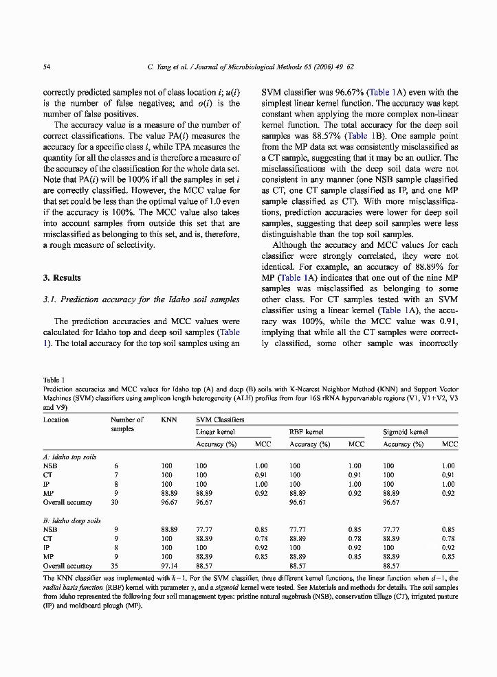
The prediction accuracies and MCC values werecalculated for Idaho top and deep soil samples (Table1). The total accuracy for the top soil samples using an

SVM classifier was 96.67% (Table 1A) even with thesimplest linear kernel function. The accuracy was keptconstant when applying the more complex non-linearkernel function. The total accuracy for the deep soilsamples was 88.57% (Table 1B). One sample pointfrom the MP data set was consistently misclassified asa CT sample, suggesting that it may be an outlier. Themisclassifications with the deep soil data were notconsistent in any manner (one NSB sample classifiedas CT, one CT sample classified as IP, and one MPsample classified as CT). With more misclassifica-tions, prediction accuracies were lower for deep soilsamples, suggesting that deep soil samples were lessdistinguishable than the top soil samples.

Although the accuracy and MCC values for eachclassifier were strongly correlated, they were notidentical. For example, an accuracy of 88.89% forMP (Table 1A) indicates that one out of the nine MPsamples was misclassified as belonging to someother class. For CT samples tested with an SVMclassifier using a linear kernel (Table 1A), the accu-racy was 100%, while the MCC value was 0.91,implying that while all the CT samples were correct-ly classified, some other sample was incorrectly

Table 1Prediction accuracies and MCC values for Idaho top (A) and deep (B) soils with K-Nearest Neighbor Method (KNN) and Support VectorMachines (SVM) classifiers using amplicon length heterogeneity (ALH) profiles from four 16S rRNA hypervariable regions (V1, V1+V2, V3and V9)

Location Number ofsamples

KNN SVM Classifiers

Linear kernel RBF kernel Sigmoid kernel

Accuracy (%) MCC Accuracy (%) MCC Accuracy (%) MCC

A: Idaho top soilsNSB 6 100 100 1.00 100 1.00 100 1.00CT 7 100 100 0.91 100 0.91 100 0.91IP 8 100 100 1.00 100 1.00 100 1.00MP 9 88.89 88.89 0.92 88.89 0.92 88.89 0.92Overall accuracy 30 96.67 96.67 96.67 96.67

B: Idaho deep soilsNSB 9 88.89 77.77 0 .85 77.77 0.85 77.77 0.85CT 9 100 88.89 0 .78 88.89 0.78 88.89 0.78IP 8 100 100 0 .92 100 0.92 100 0.92MP 9 100 88.89 0 .85 88.89 0.85 88.89 0.85Overall accuracy 35 97.14 88.57 88.57 88.57

The KNN classifier was implemented with k= 1. For the SVM classifier,radial basis function (RBF) kernel with parameter y, and a sigmoid kernelfrom Idaho represented the following four soil management types: pristine(IP) and moldboard plough (MP).

three different kernel functions, the linear function when d= 1, thewere tested. See Materials and methods for details. The soil samplesnatural sagebrush (NSB), conservation tillage (CT), irrigated pasture


labeled as CT (in this case, one of the MP samples).The errors in the classification are small, yet non-trivial. An improved analysis that achieves 100%accuracy for the SVM classifiers for the same dataset is presented below. The KNN classifiers outper-formed the SVM classifiers for the deep soil sam-ples, while they were evenly matched for the top soilsamples.

3.2. Prediction accuracies for Chesapeake Baysamples

The procedure described above for the Idaho soilsamples was independently applied to the ChesapeakeBay samples with the location-based and time-basedlabels (Table 2). The performance of the classifiers forthe Chesapeake Bay data was clearly inferior to thatfor the Idaho samples. The average accuracy was onlyabout 83%, with the accuracy for the individual clas-ses ranging from 55% to 100% (Table 2). The MCC

values ranged from 0.62 to 0.91. The performance ofthe SVM and KNN classifiers were comparable.

3.3. Optimization of the SVM classifier for ChesapeakeBay samples using model selection

Performance by the SVM classifier on the Chesa-peake Bay sediments was less than satisfactory, re-quiring further optimization. Optimization of theSVM classifier was done using model selection forthe various kernel function parameters and the pen-alty parameters (Chang and Lin, 2002). The penaltyparameter, C, is part of the error term in the SVMthat represents the rate at which the SVM "learns"from the misclassifications. A range of different ker-nel functions for the sigmoid and the RBF kernelscan be explored by varying the parameter y. Modelselection suggested the use of a SVM classifier usinga RBF kernel function with log2C=9 and log2y =2.15for Chesapeake Bay location-based classification, and

Table 2Prediction accuracies and MCC values for location-based and time-based classifications of Chesapeake Bay samples with KNN and SVMclassifiers using amplicon length heterogeneity (ALH) profiles from a single 16S rRNA hypervariable region (V1 +V2)

Sample labels Number of samples KNN SVM with RBF kernel

Accuracy (%) MCC

Samples from different locations CP 23 86.95 91.30 0.85CS 60 90.00 91.67 0.85HD 52 84.62 90.38 0.86HI 38 76.31 84.21 0.82HIM 42 83.33 83.33 0.80OC 23 82.60 78.26 0.76OM 9 55.56 55.56 0.62RB 30 70.00 76.67 0.84UP 5 60.00 60.00 0.77Overall accuracy (location) 282 81.56 84.75

Samples from different times of year Sep 99 76 85.52 88.16 0.82Dec 99 58 79.31 75.86 0.68Feb 00 50 80.00 80.00 0.81Mar 00 33 78.78 81.82 0.78May 00 15 86.66 80.00 0.89July 00 15 100.00 100.00 0.91Nov 00 35 85.71 80.00 0.77Overall accuracy (time) 282 83.33 82.62

The KNN classifiers were implemented with k=1. For the SVM classifier, only the radial basis function (RBF) kernel was used. After modelselection, parameters log2C=9 and log2y =2.15 were used for the location experiments, while log 2C=7.25 and log2y =0.75 were used for thetime experiments. The soil samples from Chesapeake Bay represented the following locations: CP=Chimney Pole, CSattle Shed, HD=HogIsland Dry, HI=Hog Island Intermediate, HW=Hog Island Wet, OCCoyster Creek Bank, OMCoyster Creek Marsh, RB=Red Bank, UP=UpperPhillips Creek.


with log2C=7.25 and log2y =0.75 for ChesapeakeBay time-based classification.

The overall accuracy (after optimization) for thelocation-based samples was 84.75%. The 49 misclas-sifications did not appear to have any perceivablepattern to them. This would suggest that the eubacter-ial community patterns in the Chesapeake Bay sedi-ments are spatially similar at the resolution of theALH profile. Alternatively, the fact that we had onlyone hypervariable region in the input may have madeit less distinguishable. We also tried alternative waysto group the location-based samples—by dividingthem into three coastal habitats, high dry Spartinamarsh, low wet Spartina marsh, and adjacent mudflats. However, this grouping did not significantlychange the performance of the classifiers (data notshown), suggesting that the tidal flux in the system ishigh enough to eliminate any distinguishing featuresin the eubacterial communities.

The overall accuracy (after optimization) for thegrouped time-based samples was 82.62%, and wastherefore comparable to that of the location-based sam-ples (84.75%). However, the misclassifications of thetime-based samples were mostly between adjacent timeperiods. In fact, 40 out of the 51 misclassifications wereto time labels that were within three months of thecorrect label. This led us to question whether a moreaccurate classifier could be built to distinguish samplesthat were sufficiently far apart (seasonal differences) intheir time labels. For example, when we built classifierstrained only with samples from July and December, theresulting SVM classifier was accurate with 94.52% ofthe test samples with those time labels. Similar resultswere observed for samples from March and September(90.83% accuracy), and from May and November(92% accuracy).

3.4. Significance of 16S rRNA hypervariable regions

The poorer performance with the Chesapeake Baydata, which interrogated only one hypervariable region,raised several questions about the relative significanceof the ALH data from the different hypervariableregions of 16S rRNA. Since ALH profiles from allthe four regions were available for the Idaho soil sam-ples (Table 1), we sought to determine the combina-tions of regions that would provide the most amount ofinformation in terms of the ability to distinguish soil

samples. This question was addressed by determiningthe accuracy of the resulting classifiers when trainedwith Idaho soil ALH profile data from every possiblecombination of the four regions. Since the number ofregions for which ALH assays are done determines thecost of the experiments, this analysis could also shedlight on the tradeoff between cost and accuracy.

The prediction accuracies were calculated whendata from different combinations of regions wereused to train both, a KNN classifier, and a SVMclassifier with RBF kernel function and a KNN clas-sifier after optimized model selection (Tables 3-5).When the profiles from only one region were utilizedto design classifiers (Table 3), the performance wasbest when the V1+ V2 region was used. For Idaho soilsamples, prediction accuracies were equally goodusing the V1 regions, with the exception of the deepsoil samples, where the SVM classifier performanceon the V1 + V2 region was marginally better than thatfor V1 region. For both top and deep soils, the worstresults were obtained with the V9 region. The accura-cies varied considerably with soil management types.For example, the NSB soil samples were best distin-guished by the SVM and KNN classifiers using theprofiles from the V1 + V2 region, or by the KNNclassifier using the profiles from the V1 region. Theclassifiers using the V9 region profiles were onlysuccessful in distinguishing the CT and IP top soilsamples, and performed poorly otherwise. In fact, theclassifiers using profiles from only the V9 region hadan overall accuracy of about 80%. Interestingly, theSVM classifiers using any of the four regions made nomisclassifications for the IP soil samples.

When two variable regions were used to designclassifiers (Table 4), using a combination of V1 andV1+ V2 regions improved the performance (for bothtop and deep soil samples) over the classifiers usingonly one of the regions. For Idaho top soil samples,prediction accuracies were equally good with a com-bination of V1 and V3 regions. The performance ofclassifiers that included the V9 region was markedlyworse than when this region was excluded (Tables 3-5). All other classifiers had reasonably high accura-cies. When three variable regions (V1, V1+ V2 andV3) were used (Table 5), the performance was goodfor all samples.

The data seems to imply that region V9 generateddata that tends to confound both the classifiers espe-

Location Number ofsamples

16S rRNA hypervariable region utilized

V1 V1+V2 V3 V9

KNN SVM KNN SVM KNN SVM KNN SVM

A: Idaho top soilsNSB 6 100.00 100.00 100.00 100.00 100.00 100.00 33.33 33.33CT 7 85.71 85.71 85.71 85.71 85.71 85.71 100.00 100.00IP 8 100.00 100.00 100.00 100.00 100.00 100.00 100.00 100.00MP 9 100.00 100.00 100.00 100.00 88.89 88.89 77.78 66.67Overall accuracy 30 96.67 96.67 96.67 96.67 93.33 93.33 80.00 76.67

B: Idaho deep soilsNSB 9 100.00 88.89 100.00 100.00 88.89 77.78 77.78 66.67CT 9 100.00 100.00 100.00 100.00 77.78 88.89 77.78 88.89IP 8 100.00 100.00 100.00 100.00 87.50 100.00 75.00 100.00MP 9 100.00 88.89 100.00 88.89 100.00 88.89 88.89 66.67Overall accuracy 35 100.00 94.29 100.00 97.14 88.57 88.57 80.00 80.00

The soil samples from Idaho represented the following four soil management types: pristine natural sagebrush (NSB), conservation tillage (CT),irrigated pasture (IP) and moldboard plough (MP). Sizes of the feature vectors for the four regions for the Idaho top soils were as follows: Vl:23; V1+V2: 31; V3: 11 and V9: 5. Sizes of the feature vectors for the four regions for the Idaho deep soils were as follows: Vl: 24; V1+V2:34; V3: 14 and V9: 7.

cially when used by itself (Table 3) or in combinationwith one of the other regions (Tables 4 and 5). How-ever, when three regions were combined, the inclusion

of V9 region had no influence on the top soil sampleswhen combined with VI and VI +V2 (Table 5). In-terestingly, the worst performance of the classifiers

Table 4Prediction accuracies for Idaho top (A) and deep soil (B) samples using KNN and SVM classifiers with linear kernel function using ALHprofiles from combination of pairs of 16S rRNA hypervariable regions


Table 3Prediction accuracies for Idaho top (A) and deep (B) soil samples using KNN and SVM classifiers with the radial basis kernel function (withmodel selection) using ALH profiles from single 16S rRNA hypervariable regions

Type Numberofsamples


[V1, V1 +V2] [V1, V3] [V1, V9] [V1 +V2, V3] [V1 +V2, V9] [V3, V9]

KNN SVM KNN SVM KNN SVM KNN SVM KNN SVM KNN SVM

A: Idaho top soilsNSB 6 100.00 100.00 100.00 100.00 83.33 100.00 100.00 100.00 83.33 100.00 83.33 83.33CT 7 85.71 100.00 100.00 100.00 100.00 85.71 85.71 85.71 100.00 100.00 100.00 85.71IP 8 100.00 100.00 100.00 100.00 100.00 100.00 100.00 100.00 100.00 100.00 100.00 100.00MP 9 100.00 100.00 100.00 100.00 100.00 88.89 88.89 88.89 100.00 66.67 88.89 66.67Overall accuracy 30 96.67 100.00 100.00 100.00 96.67 93.33 93.33 93.33 96.67 90.00 93.33 83.33

B: Idaho deep soilsNSB 9 100.00 100.00 100.00 88.89 88.89 88.89 100.00 88.89 77.78 100.00 77.78 66.67CT 9 100.00 100.00 100.00 100.00 88.89 100.00 100.00 100.00 88.89 88.89 77.78 88.89IP 8 100.00 100.00 100.00 100.00 87.50 100.00 100.00 100.00 100.00 100.00 87.50 87.50MP 9 100.00 100.00 100.00 88.89 88.89 88.89 100.00 100.00 88.89 88.89 88.89 88.89Overall accuracy 35 100.00 100.00 100.00 94.29 88.57 94.29 100.00 97.14 88.57 94.29 82.86 82.86

The soil samples from Idaho represented the following four soil management types: pristine natural sagebrush (NSB), conservation tillage (CT),irrigated pasture (IP) and moldboard plough (MP). Sizes of the feature vectors for the four regions for the Idaho top soils were as follows: Vl:23; V1+V2: 31; V3: 11 and V9: 5. Sizes of the feature vectors for the four regions for the Idaho deep soils were as follows: Vl: 24; V1+V2:34; V3: 14 and V9: 7.


Table 5Prediction accuracies for Idaho top (A) and deep soil (B) samples using KNN and SVM classifiers with linear kernel function using ALHprofiles from combination of triples of 16S rRNA hypervariable regions

Type Number ofsamples


[V1, V1 +V2, V3] [V1, V1 +V2, V9] [V1 +V2, V3, V9] [V1, V3, V9]

KNN SVM KNN SVM KNN SVM KNN SVM

A: Idaho top soilsNSB 6 100.00 100.00 100.00 100.00 83.33 100.00 83.33 100.00CT 7 100.00 100.00 100.00 100.00 100.00 100.00 100.00 100.00IP 8 100.00 100.00 100.00 100.00 100.00 100.00 100.00 100.00MP 9 100.00 100.00 100.00 100.00 100.00 100.00 100.00 100.00Overall accuracy 30 100.00 100.00 100.00 100.00 96.67 100.00 96.67 100.00

B: Idaho deep soilsNSB 9 100.00 100.00 88.89 100.00 77.78 88.89 88.89 88.89CT 9 100.00 100.00 77.79 100.00 88.89 100.00 100.00 100.00IP 8 100.00 100.00 87.50 100.00 100.00 100.00 100.00 100.00MP 9 100.00 100.00 88.89 100.00 88.89 100.00 88.89 88.89Overall accuracy 35 100.00 100.00 85.71 100.00 88.57 97.14 94.29 94.29

management types: pristine natural sagfeature vectors for the four regions forfor the four regions for the Idaho deep

The soil samples from Idaho represented the following four soilirrigated pasture (IP) and moldboard plough (MP). Sizes of the23; V1+V2: 31; V3: 11 and V9: 5. Sizes of the feature vectors34; V3: 14 and V9: 7.

were observed when all four regions (Table 1) orwhen single regions (Table 3) were used. The KNNclassifier performed better (96.69%) than the SVMclassifier (92.62%) when all four regions used. How-ever, when a combination of three regions was used,KNN performed relatively poorly with deep soil sam-ples, especially when region V9 was included.

4. Discussion

4.1. Effective classification of ALH profiles usingcomputational tools

One attractive property of SVMs is that it con-denses information in the training samples to providea sparse representation using a linear combination of asmall number of samples, referred to as the supportvectors, and only these vectors are used in the subse-quent classification. The number of support vectors istypically small compared to the total number of train-ing samples. This makes the classification task veryefficient even when analyzing large datasets contain-ing many uninformative data points. The training andoptimization phases for SVMs includes the selectionof an appropriate kernel function, selection of function

ebrush (NSB), conservation tillage (CT),the Idaho top soils were as follows: Vl:soils were as follows: Vl: 24; V1 +V2:

parameters and the regulation parameter, C. The func-tion parameters implicitly define the structure of themapped feature space, while C controls the learningrate, thereby affecting the training speed. The resultsshow that comparable accuracies were obtained withdifferent types of kernels (Table 1). Large variationsof the parameters including y for the RBF kernel hadlittle influence on the classification performance.

Both the classifiers (SVM and KNN) performedwell for Idaho soil samples. In particular, the SVMsexhibited flawless performance for the Idaho soilsamples. Our results suggest that the top soil samplesare more clearly distinguishable than deep soil sam-ples, confirming the conclusions of other researchers(Griffiths et al., 2000). This is not surprising since thesurface soil would tend to be more heterogeneous dueto soil mixing from wind and/or rain erosion. Further-more, the importation of new community membersfrom allochthonous sources would be more likely toimpact the top soil layers than the deeper ones.

Although there was no perceptible difference inthe performance of the SVM and KNN classifiers,when we looked at the aggregation of all the results,we found that the SVM classifier exhibited a mar-ginally superior performance with an average overallaccuracy of about 92%, as compared to 91% for the


KNN classifier. The standard deviation was alsosmaller with the SVM classifier, suggesting a moreconsistent performance than the KNN classifier.However, note that the KNN tool can be implemen-ted more easily than the more sophisticated SVMtool.

It may be argued that the computational tools of thetype presented here assume that the majority of ALHamplicons are common and detectable across a widerange of samples of the same type. It is not clear ifsuch an assumption is justified. However, the strongperformance of these predictors on at least some of thesoil types (e.g., natural sage brush, or irrigated pas-tures), even though the sampling was done at two orthree different locations, lends support to such a hy-pothesis. Since both the SVM and the KNN classifierscan easily deal with high dimensional data, it ispossible to extend the analyses to incorporate otheruseful features that may improve the prediction accu-racy (i.e., physical and chemical parameters of thesamples such as pH, salinity, temperature, mineraland nutrient concentrations).

4.2. Analysis of Chesapeake Bay samples

The ALH profile data from the sediment samplesfrom Chesapeake Bay were only from the V1 +V2hypervariable region of the 16S rRNA gene. Theresulting classifiers did not perform as well as theones with the data from the Idaho soils, which hadALH profiles from four hypervariable regions of the16S rRNA gene. It is likely that ALH profiles fromonly one hypervariable region (V1+ V2) is not suffi-cient for good classifications. Many other factors couldhave contributed to the difficulty in classification. Thelower performance may be due to the imbalance in thesize of the data sets in the sense that the ratio of the sizeof the largest class to the size of the smallest class is60 /5 =12 for the location-based labels and 76 /15 =5for the time-based labels. It may also be due to the factthat the community patterns of the Chesapeake Baysamples were less distinguishable from each other thanthe corresponding Idaho samples. Since the Bay sam-ples came from undisturbed and similar Spartina-dom-inated marsh sediments compared to the range of plant(native sagebrushes to crops like potatoes or alfalfa)and management systems (pasture to moldboard plo-wed) in the Idaho soil, it is not surprising that the

community patterns were similar between sites. Sedi-ments tend to be saturated most of the time driving thecommunity structure to those members that can bestsurvive or adapt to fluctuating anoxic conditions. An-other reason could be that a dense cover of Spartinamarsh grasses found at most of the sampling sites maybe driving the structure of the eubacterial communitiesassociated with the life cycle of the plants. In a relatedstudy, Hines and coworkers showed that seasonalchanges in the biogeochemical parameters in Spartinamarsh sediments of New Hampshire were aligned tothe growth phases of the marsh grasses (Rooney-Vargaet al., 1997). While the relative abundance of thesulfate-reducing bacterial community members fluctu-ated over time, members of the Desulfobacteriaceaewere found throughout the year. The dynamics of themarsh community appears to be driven by the growthcycle and physiology of the Spartina rather than bysediment temperature (Rooney-Varga et al., 1997).Therefore, it is possible that the Chesapeake Bayeubacterial communities were reflecting similar trendstoward structural homogeneity. Recent analyses fromthe Gillevet laboratory of clone libraries from re-presentative samples used in this study indicate sig-nificant overlap in eubacterial communities in allsample sites in their Chesapeake Bay study (personalcommunications).

Several interesting observations are possible fromthe analysis of the performance of the location-basedand time-based classifiers. Even though samplesobtained within a short span of time were not verydistinguishable, samples that were obtained about sixmonths apart were sufficiently distinguishable. Thus,spatial differences across sites were not as pronouncedas temporal changes within a site, which could impacthow sampling of sediments should be performed for areliable study of changes in eubacterial diversity. Thissuggests that some environmental factor other thansediment saturation, tidal washing, or anoxia may bedriving the community structure. Temperature is un-likely to be a factor since the overall sediment tem-peratures did not fluctuate greatly. The driving forcecould be the growth of the Spartina marsh grasses inthe summer and their death and decay in the winter.The carbon and nutrient influx into this ecosystem islargely due to the decay of the Spartina plants, whichmay influence the resulting nutrient status, and sub-sequently the eubacterial community composition.


Since the Chesapeake Bay study was focused onbiodiversity within the microbial communities, noenvironmental parameters were included in the anal-yses (P. Gillevet, personal communication).

4.3. Which combinations of 16S rRNA hypervariableregions are most informative?

The data suggests that a combination of profilesfrom the different regions complement each other andhelp to produce better classifiers for the whole com-munity profiles (Tables 3-5). While it may seem intu-itive that including more regions should improve theaccuracy, this was not always true. Our results suggestthat combining profiles from V1 and V1+ V2 regionsgave the most accurate classifiers (100% for both topand deep soils). Adding the profiles from region V3 tothose from V1 and V1+ V2 also gave 100% accuracy(Table 5), while adding the data from region V9 low-ered the accuracy considerably (Table 1). We proposethat profiles from different regions may be useful indifferent applications. For example, to identify thelocation of a soil sample based on its ALH pattern,the combined profiles from V1 and V1+ V2 appear tobe sufficient. On the other hand, to understand theeubacterial diversity of the whole community, the V3region profiles should be included since they showedhigh variations even within an ecosystem. It is not clearwhether the V9 region profiles provide any added valueto understand eubacterial diversity.

5. Conclusions

Microbial community profiling and their utiliza-tion to distinguish patterning among microbial eco-systems is a novel application for supervised learningtechniques such as SVMs and KNNs. Classificationtools based on these machine learning techniquesworked well for classifying or distinguishing soilsamples based on their ALH patterns. For best resultsit seemed necessary to combine the profiles fromseveral hypervariable regions of 16S rRNA genes.In particular, the profiles from region V1 + V2 weresufficient to distinguish between samples sampled atdifferent times of the year. However, they wereinadequate in distinguishing sediment communitiessampled at the same time but at different locations

in the Chesapeake Bay marshes. For the Idaho soilsamples, a combination of profiles from V1 andV1 + V2 regions provided the best results (100%accuracy). Profiles from region V3 may be includedwithout any loss of accuracy. Including region V9seemed to decrease the accuracy of the resultingclassifiers.

The fact that two different software tools were ableto learn from the data and successfully classify anddiscriminate between length heterogeneity profiles ofnew soil samples, indicates that there are hiddenpatterns in these profiles that can be discerned bythese mathematical-based tools. This work paves theway for other classification tools to be tried on similarmicrobial ecology data. It is also anticipated that thecomputational tools developed here will be useful forlarge-scale and comparative analyses of ecogenomicdata. Potential applications also exist in forensic sci-ence (Horswell et al., 2002) and environmental studies(Litchfield and Gillevet, 2002; Mills et al., 2003;Ritchie et al., 2000; Suzuki et al., 1998; Tiirola etal., 2003). The field of microbial ecology could ben-efit enormously by the development of classificationtools of the type described in this paper.

Acknowledgements

We thank Dr. Chih-Jen Lin for help with the modelselection. We also thank Ramakrishna Ruthala, SashaMiller, and Sheria King for assistance.

References

Bernhard, A.E., Field, KG., 2000. Identification of nonpointsources of fecal pollution in coastal waters by using host-spe-cific 16S ribosomal DNA genetic markers from fecal anaerobes.Appl. Environ. Microbiol. 66 (4), 1587-1594.

Bernhard, A.E., Colbert, D., McManus, J., Field, KG., 2005.Microbial community dynamics based on 16S rRNA gene pro-files in a Pacific Northwest estuary and its tributaries. FEMSMicrobiol. Ecol. 52, 115-128.

Blackwood, C.B., Marsh, T., Kim, S.H., Paul, E.A., 2003. Terminalrestriction fragment length polymorphism data analysis for quan-titative comparison of microbial communities. Appl. Environ.Microbiol. 69 (2), 926-932.

Brown, M.P., Grundy, W.N., Lin, D., Cristianini, N., Sugnet, C.W.,Furey, T.S., et al., 2000. Knowledge-based analysis of microarraygene expression data by using support vector machines. Proc.Natl. Acad. Sci. U. S. A. 97 (1), 262-267.

C. Yang et al. /Journal of Microbiological Methods 65 (2006) 49-62

61

Burges, C.J.C., 1998. A tutorial on support vector machines forpattern recognition. Data Mining Knowledge Discov. 2 (2),121-167.

Chang, C.-C., Lin, C.-J., 2001. LIBSVM: a Library for SupportVector Machines. http://www.csie.ntu.edu.tw/-cjlin/libsvm.

Chang, C.-C., Lin, C.-J., 2002. A practical guide to support vectorclassification. http://www.csie.ntu.edu.twt-cjlin/papers/guide/guide.pdf.

Cocolin, L., Manzano, M., Cantoni, C., Comi, G., 2001. Denaturinggradient gel electrophoresis analysis of the 16S rRNA gene V1region to monitor dynamic changes in the bacterial populationduring fermentation of Italian sausages. Appl. Environ. Micro-biol. 67 (11), 5113-5121.

Collobert, R., Bengio, S., 2001. Svmtorch: support vector machinesfor large-scale regression problems. J. Mach. Learn. Res. 1,143-160.

Cristianini, N., Shawe-Taylor, J., 2000. Support Vector Machines.Cambridge University Press.

Dunbar, J., Ticknor, L.O., Kuske, C.R., 2000. Assessment of mi-crobial diversity in four Southwestern United States soils by 16SrRNA gene terminal restriction fragment analysis. Appl. Envi-ron. Microbiol. 66 (7), 2943-2950.

Dunbar, J., Ticknor, L.O., Kuske, C.R., 2001. Phylogeneric spec-ificity and reproducibility and new method for analysis ofterminal restriction fragment profiles of 16S rRNA genes frombacterial communities. Appl. Environ. Microbiol. 67 (1),190-197.

Dunbar, J., Barns, S.M., Ticknor, L.O., Kuske, C.R., 2002. Empiricaland theoretical bacterial diversity in four Arizona soils. Appl.Environ. Microbiol. 68 (6), 3035-3045.

Efron, B., Tibshirani, R., 1993. An Introduction to the Bootstrap.Chapman and Hall, New York, London.

Furey, T.S., Cristianini, N., Duffy, N., Bednarski, D.W., Schummer,M., Haussler, D., 2000. Support vector machine classificationand validation of cancer tissue samples using microarray ex-pression data. Bioinfonnatics 16 (10), 906-914.

Griffiths, RI., Whiteley, A.S., O'Donnell, A.G., Bailey, M.J., 2000.Rapid method for coextracrion of DNA and RNA from naturalenvironments for analysis of ribosomal DNA- and rRNA-basedmicrobial community composition. Appl. Environ. Microbiol.66 (12), 5488-5491.

Hastie, T., Tibshirani, R., Friedman, J., 2001. The Elements ofStatistical Learning. Springer, New York.

Hill, J.E., Seipp, R.P., Betts, M., Hawkins, L., Van Kessel, A.G.,Crosby, W.L., et al., 2002. Extensive profiling of a complexmicrobial community by high-throughput sequencing. Appl.Environ. Microbiol. 68 (6), 3055-3066.

Horswell, J., Cordiner, S.J., Maas, E.W., Martin, T.M., Sutherland,K.B.W., Speir, T., et al., 2002. Forensic comparison of soils bybacterial community DNA profiling. J. Forensic Sci. 47 (2),350-353.

Hsu, C.-W., Lin, C.-J., 2002. A comparison of methods for multi-class support vector machines. IEEE Trans. Neural Netw. 13,415-425.

Hua, S., Sun, Z., 2001. Support vector machine approach forprotein subcellular localization prediction. Bioinformatics 17(8), 721-728.

Joachims, T., 1997. Text categorization with support vectormachines: learning with many relevant features. Proc of the10th European Conference on Machine Learning, ECML-98.

Joachims, T., 1999. Making Large-Scale SVM Learning Practical.MIT-Press, Cambridge, MA.

Karchin, R., Karplus, K., Haussler, D., 2002. Classifying G-proteincoupled receptors with support vector machines. Bioinfonnatics18 (1), 147-159.

ICnerr, S., Personnaz, L., Dreyfus, G., 1990. Single-layer learningrevisited: a stepwise procedure for binding and training a neuralnetwork. Proc of Neurocomputing Algorithms, Architecturesand Applications. Springer-Verlag.

Lee, Y., Lee, C.K., 2003. Classification of multiple cancer types bymulticategory support vector machines using gene expressiondata. Bioinformatics 19 (9), 1132-1139.

Lin, K., Kuang, Y., Joseph, J.S., Kolatkar, P.R., 2002. Conservedcodon composition of ribosomal protein coding genes inEscherichia coli, Mycobacterium tuberculosis and Saccharomy-ces cerevisiae: lessons from supervised machine learning infunctional genomics. Nucleic Acids Res. 30 (11), 2599-2607.

Litchfield, C.D., Gillevet, P.M., 2002. Microbial diversity and com-plexity in hypersaline environments: a preliminary assessment.J. Ind. Microbiol. 28, 48-55.

Ludwig, W., Schleifer, K.H., 1994. Bacterial phylogeny based on16S and 23S rRNA sequence analysis. FEMS Microbiol. Rev.15 (2-3), 155-173.

Maidak, B.L., Cole, J.R., Parker Jr., C.T., Garrity, G.M., Larsen, N.,Li, B., et al., 1999. A new version of the RDP (RibosomalDatabase Project). Nucleic Acids Res. 27 (1), 171-173.

Matthews, B.W., 1975. Comparison of predicted and observedsecondary structure of T4 phage lysozyme. Biochim. Biophys.Acta 405, 442-451.

Michie, D., Spiegelhalter, D., Taylor, C. (Eds.), 1994. MachineLearning, Neural and Statistical Classification. Ellis HorwoodSeries in Artificial Intelligence, Ellis Horwood.

Mills, D., Fitzgerald, K., Litchfield, C., Gillevet, P., 2003. A com-parison of DNA profiling techniques for monitoring nutrientimpact on microbial community composition during bioremedi-ation of petroleum-contaminated soils. J. Microbiol. Methods 54(1), 57-74.

Noble, W.S., 2004. Kernel Methods in Computational Biology. MITPress, Cambridge, MA.

Olsen, G.J., Lane, D.J., Giovannoni, S.J., Pace, N.R., Stahl, D.A.,1986. Microbial ecology and evolution: a ribosomal RNA ap-proach. Annu. Rev. Microbiol. 40, 337-365.

Osuna, E., Freund, R., Girosi, F., 1997. Training support vectormachines: an application to face detection. Proc of the IEEEConf. Computer Vision and Pattern Recognition.

Pace, N.R., Olsen, G.J., Woese, C.R., 1986. Ribosomal RNAphylogeny and the primary lines of evolutionary descent. Cell45 (3), 325-326.

Pavlidis, P., Wapinski, I., Noble, W.S., 2004. Support vector machineclassification on the web. Bioinfonnatics 20 (4), 586-587.

Ritchie, N.J., Schutter, M.E., Dick, R.P., Mymld, D.D., 2000. Useof length heterogeneity PCR and fatty acid methyl ester profilesto characterize microbial communities in soil. Appl. Environ.Microbiol. 66 (4), 1668-1675.


Rooney-Varga, J.N., Devereux, R., Evans, R.S., Hines, M.E., 1997.Seasonal changes in the relative abundance of uncultivatedsulfate-reducing bacteria in a salt marsh sediment and in therhizosphere of Spartina alterniflora. Appl. Environ. Microbiol.63 (10), 3895-3901.

Riiping, S., 2002. mySVM. http://www-ai.cs.uni-dortmund.de/SOFTWARE/MYSVM/.

Scholkopf, B., Sung, K., Burges, C., Girosi, F., Niyogi, R, Poggio,T., et al., 1997. Comparing support vector machines with Gauss-ian kernels to radial basis function classifiers. IEEE Trans.Signal Process. 45 (11), 2758-2765.

Sturn, A., Quackenbush, J., Trajanoski, Z., 2002. Genesis: clusteranalysis of microarray data. Bioinfonnatics 18 (1), 207-208.

Suzuki, M., Rappe, M.S., Giovannoni, S.J., 1998. Kinetic bias inestimates of coastal picoplankton community structure obtained

by measurements of small-subunit rRNA gene PCR ampliconlength heterogeneity. Appl. Environ. Microbiol. 64 (11),4522-4529.

Tiimla, M.A., Suvilampi, J.E., Kulomaa, M.S., Rintala, J.A., 2003.Microbial diversity in a thermophilic aerobic biofilm process:analysis by length heterogeneity PCR (LH-PCR). Water Res. 37,2259 – 2269.

Vert, J.-R, 2002. Support vector machine prediction of signal pep-tide cleavage site using a new class of kernels for strings. ProcPacific Symp Biocomputing.

Zheng, G., George, E.O., Narasimhan, G., 2003. Neural networkclassifiers and gene selection methods for microarray data onhuman lung adenocarcinoma. Proc Critical Assessment ofMicroarray Data (CAMDA), Raleigh, NC.

Documents

Journal SCIENCE CLDIRECT 'Microbiological … C. Yang et al. /Journal of Microbiological Methods 65 (2006) 49-62 The computational analyses were performed on two different sets of