Journal of Theoretical and Applied Information Technology ...informatika.stei.itb.ac.id/~rinaldi.munir/Penelitian/Makalah_JATIT... · accurate. The studies above did not describe

Journal of Theoretical and Applied Information Technology 15th December 2017. Vol.95. No 23

© 2005 – ongoing JATIT & LLS

ISSN: 1992-8645 www.jatit.org E-ISSN: 1817-3195

6454

A NEW METHOD FOR ANALYZING CONGESTION LEVELS BASED ON ROAD DENSITY AND VEHICLE SPEED

M.D. ENJAT MUNAJAT1, DWI H. WIDYANTORO2, RINALDI MUNIR3

School of Electrical Engineering and Informatics

Institut Teknologi Bandung, West Java, Indonesia

E-mail: [email protected], [email protected], [email protected]

ABSTRACT

Congestion remains as an important issue to date, and it is continuously investigated by experts in order to find solutions in the process of information dissemination to road users. The existing research was more concerned on detecting vehicles and road rather than congestion, thus there has been no clear definition of congestion offerred. What really happened was that vehicle accumulation will always be referred to as congestion, although it is not necessarily the case, thus the information about congestion condition becomes inaccurate. Moreover, the existing research mainly viewed the vehicle speed aspect as the basis of congestion level estimation. Other researchers used GPS and probe detectors, but there has been much limitation despite such equipment. On average, the research carried out was only focused on the number of vehicles at a given frame as the basis for density/congestion calculation. In fact, congestion is also determined by road density and vehicle speed in a given period. Therefore, it is necessary to find a way that can display the information about road condition and congestion in a factual, timely manner. In this paper, we present two novel methods in the context of congestion detection employing information about road density and vehicle speed. Road density defines the extent to which road area is occupied by vehicles, while vehicle speed sees how fast vehicles pass a given frame. Thus, the information of both helps define the levels of vehicle congestion on a road. Based on the experiment conducted on an in-city road, this method was found to be accurate in defining the levels of congestion, starting from light, jam to heavy-jam traffic. To corroborate the argumentation of the congestion conditions, calculation using Fuzzy model was conducted given that the congestion levels are not measurable in an exact manner (light (macet ringan), jam (macet sedang), heavy-jam (macet berat) and total traffic gridlock (macet total)), thus the information obtained is more accurate. The method developed does not require high cost, yet it is quite effective in presenting congestion information in a quick, real-time, accurate way. Keywords: Traffic Congestion, Vehicle Detection, Vehicle, Tracking, Vehicle Density, Vehicle Speed

Detection, Image Processing 1. INTRODUCTION

Congestion has quite a few negative impacts such as noise, pollution emission, accidents and wasted time in traffic, which are acknowledged as an issue. On the other hand, rooting out traffic congestion is not an option. Some solutions to break up congestion, one of which is traffic management, are required. Various methods have been developed to oversee the roads, and eventually detect congestion. The systems developed always have 3 (three) main paramenter stages, namely (1) vehicle detection, (2) vehicle tracking, (3) vehicle and trajectory pattern classification. For vehicle detection, most methods [1], [2], [3], [4], [5] used stationary cameras,

allowing the detection of the vehicles desired through image.

Li et al. [6] attempted to detect congestion by utilizing vehicle sensors in taxis in Shanghai, China. As shown in Figure 1, the model developed by [6] was concerned more on the understanding of congestion monitoring performance with the lack of information provided by the sensors. Similarly, [7] used a probe detector to calculate the levels of road congestion using GPS in monitoring the vehicle motions. A different approach was conducted by Hsu et al [8]. As shown in Figure 2, [8] leaned toward using entropy (square blocks) as a template for calculating the number of passing vehicles.




6455

They attempted to map background areas by setting boundaries in the form of squares by using Gussian feature. The experiments tended to be conducted in the daytime when the illumination was good. And this is not everything. Research on congestion has expanded to mobile application as well. Let us say a number of names such as Google Maps and Waze that use user GPS feature in the process, as well as Macetter.us and Lewatmana.com that use CCTV camera screenshoots forwarded to users. Unlike the previously mentioned studies, the other studies did not specifically detect congestion. They only detected objects like what has been conducted by [9], [10], [11]; or detected moving objects like what has been conducted by [12], [13], [14], [15] and [8]; or detected the motion of objects like what has been conducted by Morris et al. [16] and Chen et al [17].

Figure 1. Li’s Method [6]

Figure 2. Hsu’s Method [8]

Next, research in the field of road majorly uses the RGB function with Grey-Level solely to determine lane detection through Hough-Transform and canny detection processes. The threshold value is manually determined. Some research was also only caught up in mapping in the form of Inverse Perspective Mapping (IPM), other than Kalman Filter, that seems to be quite favored by lane researchers, to estimate the lane form.

Some other studies also used the positions of certain virtual points to determine the positions of signs and roads like the one carried out by Chen [17]. In his research, Chen [17] tended to use detector points (Figure 3) that virtually calculated every vehicle passing on those virtual points. If virtual points are used in the calculation using Kalman Filter [12], it can be ascertained that the result will be in probability form and it is not close to the real condition as only point samples are taken, and then he [17] tried to map the future form. To support the fact that this is only a statistical analysis, [17] attempted to show the results of virtual point reading in the form of number of vehicles recorded every day, with which efficient and inefficient days can be determined. It is arguable that the research [17] still used manual measures/equations to determine the fit form, while Kalman Filter is a form of statistical equations whose accuracy is still undeterminable.

Figure 3. Chen’s Method [17]

Figure 4. Chen’s Result Data [17]

The research conducted by [18], [15] and [14] endeavoured to conduct vehicle detection, tracking and classification by using one or a number of camera video(s). The results showed that the detection ability was fairly good with an average accuracy of up to 80% and classification of up to 91% [15] in a shadowy condition. However, the tracking results seemed to be not maximal due to

‐

20,000

40,000

60,000

80,000

100,000

120,000

1 2 3 4 5 6 7

Vehicle‐HoursofDelay

Days

DelayfromInefficiency,ExcessDemand

Inefficiency ExcessDemand

Section

Direction of Flow

Detector




6456

some issues in the detection (such as vehicle overlap, vehicle shadows, weather factor, illumination, etc.), which resulted in errors in the reading in the tracking process, and automatically the congestion identification resulted was not accurate.

The studies above did not describe the criteria of congestion, thus vehicle accumulation has always been referred to as congestion, although this is not necessarily the case, making the reading of the congestion conditions inacurate. Moreover, the existing research mainly viewed the vehicle speed aspect as the basis of congestion level estimation. Other researchers used GPS and probe detectors, but there has been much limitation despite such equipment, including: (1) its tendency to require high cost and participation of users as the active informants for congestion detection, and (2) the needs of complicated setup. On average, the research carried out was only focused on the number of vehicles at a given frame as the basis for density/congestion calculation. In fact, congestion is also determined by road density and vehicle speed in a given period.

Based on the studies having been described, this paper explains the method that has the ability of congestion detection based on two novel approaches, namely: (1) traffic by road-density, and (2) traffic by vehicle speed. Traffic by road-density approach views the vehicle density compared to the area of the road used as the monitoring object. Thus, this comparison is used as the basis for vehicle density determination. The next approach is traffic by vehicle-speed, which views more the average speed of passing vehicles per time unit. These two approaches are then combined into fuzzy model and the result becomes accurate for determining the actual congestion condition. The method developed does not require high cost, yet it is quite effective in presenting congestion information in a quick, real-time, accurate way. To corroborate the argumentation of the congestion conditions, calculation using Fuzzy model was conducted given that the congestion levels are not measurable in an exact manner (light traffic (macet ringan), medium traffic (macet sedang), heavy traffic (macet berat) and total traffic gridlock (macet total)), thus the information obtained is more accurate.

2. RELATED WORKS

There have been a large number of studies focusing on vehicle detection and tracking, but none of them focused on congestion identification. In the following, some studies related to object detection, vehicle tracking and traffic monitoring will be discussed.

2.1 Object Detection The studies on vehicle detection have been

fairly matured, as seen in Table 1. One of which is [18], which used multicam. The objective of [18] is to recover the event missed by one camera, and by using other camera(s), it is expected that the event can be captured. [18] even used up to 15 cameras in the process of reading passing vehicles by experimenting using 1, 2, 3 to 15 vehicles. It is evidenced by the reading results that reached 95.2% vehicle validation when the proposed method was used, but lowered to 60% when the proposed method was not used.

Table 1. General methods of vehicle detection, tracking and classification

Vehicle Detection Vehicle Tracking

Gaussian Mixture Model [19], [20], [2], [3], [21], [22]

AdaBoost [19], [20], [2]

Haar-Like Feature [19], [20], [2] Kalman Filter [15], [14], [13], [20], [2],[3],[21]

Kalman Filter [15], [14], [13], [20], [2],[3],[21]

Support Vector Machine (SVM) [19],[2],[5],[23]

AdaBoost [19], [20], [2]

Similarly, Jun-Wei Hsieh et al. [15]

defines a new feature called “vehicle linearity” to classify types of vehicles. This new feature is highly useful for distinguishing “truck van” from “truck”, even without the need to use 3-Dimensional information. The method offerred by [15] is actually similar to the Gaussian Mixture Model (GMM) process in [19], [20], [2], [3], [21], [22] that is widely applied. The process involved in GMM includes the recognition of background and obervation of the motion of foreground at every frame. This method is in fact fairly matured and known to a number of similar studies such as [19], [20], [2], [3], [21], [22]. Different from the testing carried out by Jun-Wei Hsieh et al. [15], they undertook the testing on roads that tended to be moderate in density. The results show that the method offerred by Jun-Wei Hsieh et al. [15] had a fairly good detection ability with an average accuracy of up to 80%. Afterwards, [15] developed




6457

the method to enable classification. As a results, vehicle classification was possible to be done to a level of 91%, even in a shadowy condition. The process used by [15] tended to reconstruct the Gaussian Mixture Model process in [19]-[22] by adding some sort of boundaries to every lane, and these boundaries then cut the shadow of every vehicle passing them, increasing the precision in a shadowy condition.

Beymer et al. [14] in 1997 conducted the same research on vehicle detection. They [14] claimed that the method offerred (at that time) was the best. Beymer et al. [14] tried to detect vehicle using stationary camera. In this research, Beymer et al. [14] utilized a tracker in the Texas Instruments C40 DSPs (Digital Signal Processing) network. In this case, [14] seemed to use built-in Chips with additional algorithm for vehicle detection process. In the experiment, Beymer conducted an experiment using 44-hour-long traffic videotape. At a glance, the method employed by Beymer et al. [14] did appear to have referred to the Gaussian Mixture Model (GMM) method in [19], [20], [2], [3], [21], [22] and had something in common with the method employed by Jun-Wei Hsieh et al. [15]. It also seemed that the research by Beymer et al. [14] was a fairly influental study that inspired another similar study [15]. With their method, Beymer et al. showed quite significant results. The accuracy of the vehicle reading even reached 94.2% at most and 73.9% at least.

Similar research was carried out by W.-L. Hsu, H.-Y.M. Liao [8], where they [8] suggested a vision-based traffic monitoring system that is able to do real-time parameter extraction. Entropy was used as the measure underlying the calculation of traffic flow and vehicle speed. Based on the entropy, some key traffic parameters such as traffic flow, speed difference between vehicles and traffic queue can be determined real-time. The concept developed tended to be the same as the concept of others. They [8] attempted to map the background area by making square-shaped boundaries and conducted calibration on them. If the background area was occupied, the foreground would be read per frame and the number of vehicles passing them would be counted. This process seemed to use Gaussian process, in which the background and foreground are recognized by using Grey-Scale process. The results of the experiment show a very good condition, where they [8] were able to readup to 100% in a certain condition, namely bright condition.

2.2 Vehicle Tracking and Traffic Monitoring Intelligent transportation system has been

garnering much attention in the past decade. Vehicle detection is the main task in this area, and vehicle calculation and classification are two essential applications. In the field of vehicle tracking, some used sensors as shown in Table 2, and some other used the development of matured approaches such as Kalman Filter, Ada Boost and so forth. However, the methods that tended to be used in the tracking process were also used in the detection process, as those methods principally were interconnected. Only the development of the methods was left in the hand of each researcher.

Table 2. Comparison of Sensors for Vehicle Detection

[19]

Sensing Modality

Perceived Energy

Raw Measurement

Units Recognizing Vehicles vs. Other Objects

Radar

Milimeter-wave radio signal (emitted)

Distance Meters Resolved via tracking

Lidar

600-1000 nanometer-wave laser signal (emitted)

Distance Meters

Resolved via spatial segmentation, motion

Vision Visible light (ambient)

Light intensity Pixels Resolved via appearance, motion

As noted previously, traffic management process always involves 3 processes, namely: (1) vehicle detection, (2) vehicle tracking and (3) vehicle classification. Therefore, one process and another are interlinked. The methods developed will always be related and complementary to each other. For example, some tracking methods discussed below basically also involve detection process.

The research conducted by Shunsuke Kamijo et al. [24] was more concerned with congestion monitoring process and accident detection around intersections. Although [24] also involved detection process in the research, it focused more on the tracking process. Shunsuke [24] adopted Spatio Temporal – Markov Random Fields (ST-MRF) based on Hidden Markov Model (HMM), where [24] used pixel scheme sized 8 x 8 pixels. The experiment was carried out at a jammed intersection for a duration of 25 minutes. Basically, the research [24] leaned more toward object detection. Object detection at every frame using Spatio Temporal-Markov Random Fields (ST-




6458

MRF) allowed the system to do more things, from tracking to learning the various behavior patterns of each vehicle. For example, traffic collision, high number of passing vehicles that cause congestion, illegal U-turns or reckless driving could be recognized well. Although the method conveyed by [24] was quite simple, but in its time (2000), it apparently was fairly good at tracking, resulting an accuracy level of 93-96%.

Other than from the abovementioned research, we also obtained information from youtube.com for some similar published applications. An example brought forward in this research is shown in Figure 5 [26], which seems to have been in the commercial production stage. In this video, some vehicle detection stages are shown in a polygonal format. This vehicle detection was used for calculating the speed at 8 two-way roads. It did not specifically detect the road capacity and the levels of congestion, and it only played on roads with traffic flow that was light to jam, but not heavy-jam.

On the other hand, the research [27] as shown in Figure 6 measured a number of traffic parameters such as number of vehicles, vehicle classes (motorcycles, light vehicles and heavy vehicles) and vehicle speed. This video also tried to estimate the number of vehicles, which could be used to predict traffic congestion. This system claimed to be able to work under varied weather conditions (clear, cloudy, snowy). However, we found that it only detected vehicles of certain sizes, and then counted the number. It appeared to be quite good, but it was still unable to detect the congestion conditions. Furthermore, this research also only played in the area of roads with traffic flow that was light to jam, but not heavy-jam.

Figure 5. Vehicle speed detection [26]

Another video from [28] as shown in Figure 7 claimed that it was able to detect urban traffic, count the number of vehicles, classify types of vehicles and road boundaries, and vehicle speed. However, the researchers found that the system developed could only do vehicle detection and tracking. In the light to jam condition, the system found it difficult to determine the positions of the vehicles and the tendency of error was fairly high considering the video displayed.

Figure 6. Detection of vehicle types and counting of the number of vehicles [27]

Furthermore, the video in Figure 8 [29]] show that the processing application was intended to count the number of passing vehicles by using the boundaries manually created, and then those vehicles were classified into two types of vehicles, namely car and motorcycle. In the video shown [29], the system was able to sort two-wheeled vehicles from four-wheeled vehicles fairly well. However, this system was far from being able to be used for detecting road congestion as the area of detection used was fairly small in size and the video shown was recorded at light traffic.

Figure 7. Vehicle detection [28]

As shown in Figure 9, in the video of

research [30] they claimed that their system was




6459

able to classify vehicles and the number of vehicles. In light traffic, the system was able to detect the area quite well. But in heavy-jam traffic, the system faced a difficulty in the detection process.

Figure 8. Detection of the types and number of vehicles [29]

(a) Fluent Condition (b) Smooth Condition

Figure 9. Classification of vehicles and calculation of the number of vehicles [30]

As seen in Figure 9 (a), the system’s detection was quite good. But as shown in Figure 9 (b), the number of vehicles increased, which caused overlapping in the vehicle detection. The condiction was even worse in Figure 9 (c), where the overlapping was obvious.

3. PROPOSED METHODS

Based on the explanation above, we proposed a novel method for measuring the levels of congestion by using a single surveillance camera. The camera setting used is shown in Figure 10.

Figure 10. Camera Position Setting

The surveillance camera was set at a

certain height, and the range of vision was set in such a way in order that the camera could capture the actual conditions. Here, the camera recorded the road conditions. The result of the recording was motions per frame, which then was used for analysis. Figure 11 shows the system conditions proposed for breaking down the vehicle congestion information. Based on the camera reading in Figure 6, the image format was changed into greyscale. This process was required as it would be easier for the system to read dark and bright colors of the images captured. This was used as the basis for the calculation of the density and for the detection of vehicle motions.

Figure 11. System Overview

Each process is outlined in subchapter 3.1 and 3.2 as shown in Figure 12. Process of Density Identification and in Figure 13. Traffic Flow by Vehicle.

(c)Jammed Condition

Camera Reading Results (fps)

Converting image into greyscale format

Process of congestion detection by

Road-Density

Process of congestion detection by

Vehicle-Speed

Congestion Level Analysis = Road Density + Vehicle

Speed

Camera pole heightCamera pole heightCamera pole height

Camera’s vision range on road




6460

3.1. Process of Indentification of the Levels of Congestion by Road-Density

The system developed processed the levels of road congestions by leveraging the information obtained from the camera reading results in the greyscale format (Figure 12). Firstly, the system had to be able to read the Region of Interest (ROI), which is the road area. ROI was manually determined by placing the ROI based on certain coordinates (in this case, we used 4 coordinates to set the road area). After determining the ROI area, by utilizing the greyscale technique, dark and bright areas were obtained. The dark area represented the ROI, while the bright area represented the moving objects. By setting the levels of darkness and brightness in such a way (thresholding process), smooth dark and bright areas were obtained. Thus, the distinction between the road and the passing vehicles became clearer.

Then, by counting the number of blackpixel and whitepixel, the system could read the percentage of the road dark area (background) blocked by the bright area of the vehicles (foreground). To determine the density, we used equation (1) below.

Figure 12. Process of Density Identification

∑

∑ ∑ 100%

(1)

= level of road density

numberofvehiclepixels blobs /foreground

numberofroadpixels/background

Meanwhile, to determine the road density, we used the percentage of RoadDensity as function ‘f(d)’ based on the criteria formulated in equation (2) below.

f (d)

Low Density, RoadDensity ≤30%

Mid Density, 30%< RoadDensity ≤65%

High Density, RoadDensity 65%

(2)

The details of the process are illustrated in a flow form as seen in Figure 12.

3.2. Process of Identification of the Levels of Congestion by Vehicle Speed

As described in previous section, it is not enough to measure the levels of congestion based on the road density only. Vehicle speed is an important parameter that must also be measured in addition to the density. The vehicle speed is calculated by leveraging the previous process.

As shown in Figure 13, the ROI, that has been determined in the previous process, was devided into 4 (four) parts. The first part was intended to identify moving objects based on the foreground (white area), or known as blobs (Figure 14). The clearly seen blobs area is a representation of moving objects, namely cars. Blobs are more polygonal, while to facilitate identification process, a standard shape is required. In the shape standardization process, we chose rectangle, which only has 4 sides but all of the sides are quite representative in describing the outline of each vehicle as seen in Figure 18 (c,f).

In the process of transformation of polygon to rectangle, the equation from H. Freeman and Shapira, 1975 [25] was used. They [25] used algorithm to detect blobs and encapsule them with the nearest polygonal shape, which was processed further to be a more ordered rectangle based on the polygonal vertexes identified.

Afterwards, the speed of each moving object represented by rectangle was calculated. The speed was calculated in the tracking process. In this case, we used Kalman Filter equation [12]. However, Kalman Filter equation only detects the motions of a pixel instead of a rectangle. Thus, in the following process, the center of the rectangle was determined by drawing two diagonal lines of




6461

the rectangle, and then the center was found at the intersection of the diagonal lines. The motion of this central point was used as the base for determining the vehicle speed (equation (3)). The average speed of the vehicle object at time ‘i’ was be calculated based on equation (4) below.

Figure 13. Flow of Traffic by Vehicle-Speed

(a) (b)

Figure 14. Process of sorting out background from foreground by using the threshold feature; (a) the vehicle condition on road; (b) the result of thresholding process

with dark color representing the road condition and bright color representing the vehicle object;

_

#

(3)

. ∑_

1 (4)

Distance is the gap between the start point and the finish point of the vehicle’s trip, while #Frame is the number of frames required by a vehicle to complete a trip from the start point to the finish point. The last activity, which was counting the number of passing vehicles, will be easier to carry out if the vehicle recognition in the initiation phase is correct in process. In this case, the first three fourth of the frame length was used as the start point and finish point of the calculation. In this process, every vehicle passing the start point (the first three fourth of the frame length) was counted and validated at the finish point. If in the initiation process (the first quarter of the frame length) the system is able to sort out the identity of each moving vehicle object, the system will keep on monitoring the number of vehicle detected at the initiation point, which will be tracked and counted until reaching the finish point of the frame. In equation (4), we defined average speed as a vehicle speed function ‘f(vs)’ as shown in equation (5) below.

f (vs)Low, Av.Speed ≤ 30Km/H

Mid, 30Km/H< Av.Speed ≤ 50Km/H

High, Av.Speed 50Km/H

(5)

Equation (5) serves as the basis for the determination of the levels of average speed of passing vehicle per a given time unit.

3.3. Traffic Congestion by Road Density and Vehicle Speed

This subchapter will discuss the combination of the information of road density and vehicle speed. A good congestion model tends to combine the information of average speed and density per time unit. This information will reflect the actual congestion conditions. The approach employed is illustrated in Figure 15. It can be seen that the level of congestion is a combination of the information described in the previous subchapters.




6462

Thus, the information generated can be assured to be more accurate.

Figure 15. Trafic Congestion Model

As explained in the previous chapter, there

is no definitive definition for the level of congestion. The level of congestion has only been judged according to vision, but this is clearly inaccurate, and the role of humans is required to determine the levels of congestion. In this research, we tried to approach using fuzzy model in order to identify the conditions of congestion accurately. The definition applied was vehicle speed and road density as illustrated in Table 3.

Table 3. Congestion Condition Definition

Average Speed (Km/H)

Roa

d D

ensi

ty (

%) Low Speed Mid Speed

High Speed

Low Density Light Light Light

Mid. Density Jam Jam N/A

High Density Heavy Jam Heavy Jam N/A

According to Table 3, we put the

conditions of congestion as the following fuzy algorithm. IF RoadDensity is X AND Average_Speed is Y THEN Congestion_Level is Z

However, in some conditions, we assumed that there was a condition of impossibility occured (N/A). This condition happens when the speed is high and the density is low, as well as when the speed is high and the density is moderate.

4. EXPERIMENTS, RESULTS AND EVALUATION

4.1. Traffic by Road Density

According to the method proposed in subchapter 3, with the ROI coordinates having been determined manually, the system had to determine

the start line and finish line of the object’s trip in ROI as well. We intentionally prepared the lines to anticipate the desired ROI only. The result of greyscale image reading from the surveillance camera was in the from of video frames, which would be included in the processing system. The video resulted was broken per frame to facilitate the reading process. The system reading resulted in a green area as shown in Figure 16 (a), (c), (c), which tended to follow the road. The green area was then used as the actual road ROI basis. Every passing vehicle was ensured to pass the ROI area, and it was processed in the next stage. The greyscale image was used as the processing basis by setting the appropriate threshold value to determine the area of moving objects.

To create a good distinguishing effect, the

thresholding feature was used. By using this feature, the image is converted into greyscale format, making the lines between background and foreground clearer. The thresholding values applied were 30 for the lower limit and 50 for the upper limit. The image resulted from the thresholding (greyscale) was then used in the process of moving object recognition (foreground/white pixel/blobs). The result of thresholding is shown in Figure 14.

(a) (b)

(c) (d)

(e) (f)

Figure 16. (a),(c),(e) Process of identification of road area (ROI); (b) Fluent road condition; (d) Smooth road

condition; (f) Jammed road condition.

Process of detection of congestion based on Street-Occupancy

Process of detection of congestion based on the Average Speed

Traffic Congestion Modelling = Street Occupancy +

Average Speed




6463

Figure 14 shows that the dark color represents stationary condition, which is the road, while the bright color (white) represents moving objects (vehicles like motorcycles or cars). After going through the thresholding process, the distinction between the road object and vehicle object became clearer. For the real condition of the reading result agains the thresholding feature, we conducted reading on the road conditions as shown in Figure 16. This recording was conducted in Dago area – Bandung City – West Java, Indonesia, which was categorized into a jammed area. Figure 16 shows the road area occupied by vehicles (black color represents the road, and white color represents the vehicle).

(a) (b) (c) Figure 17. Road Density Reading Result: (1) Low-

Density Condition; (b) Mid-Density Condition; (c) High-Density Condition

Using the mathematical equation proposed (Equation (2)), the comparison between the white area and black area could be found out easily. Road density determined the levels of vehicle density per certain time unit. We could analogize this level of density as on-road vehicle density. The higher the on-road vehicle density, the denser the road condition was. Conversely, the lower the on-road vehicle density, the more fluent the road condition

was. Density is illustrated in Figure 16 Relationship between road density and passing vehicles. If the density is higher, the traffic condition will definitely be more jammed. Road density was determined based on the ROI area represented by parallelogram-shaped green area as shown in Figure 16.

The road density reading result can be seen in detail in Figure 17. There are three reading conditions, namely the condition shown in Figure 17 (a), in which the density condition tends to be low, with the road appearing rather empty, thus the level of density of less than or equal to 30% will be categorized into low-density condition; the condition shown in Figure 17 (b), which is the mid-density condition, in which the road is fairly occupied with level of density of over 30% but below 65%; and condition shown in Figure 17 (c), which is high-density condition, with level of density of over 65%. At a glance, conditions (b) and (c) seem to be similar. Granted, if only the density is considered, the reading conditions become ambigous. Thus, in this research, we also considered the importance of speed calculation to determine the actual condition.

4.2. Traffic by Vehicle Speed

As described in equation (3), measurement of vehicle speed based on rectangular object was carried out. The measurement of speed was conducted per certain time unit to obtain the desired average value of speed. The speed is measured based on the central point of the rectangle as seen in Figure 18. The problem is, we had to be able to track the same one rectangular area in every motion. This process was not easy given that in a certain density condition, there would be many objects (rectangles) that moved. Certainly, the system would find it difficult to recognize the position of the same rectangle object. As for the rectangle fuction, we used the equation by H. Freeman and Shapira, 1975 [25], that used blobs detection algorithm, and then encapsulated it with the nearest polygonal figure to be processed into a more ordered rectangle based on the polygonal vertexes identified. Algorithm [25] was fairly good at recognizing blobs shapes, making it easy for envelopement by rectangles, which is evidenced in Figure 18. Thus, it was easier for us to track.

The next challenge was tracking the same

rectangle. To recognize the same object, we used Kalman Filter equation (Equation (6)) [12]. Ideally, Kalman only recognizes a point instead of a rectangle. Thus, with a simple algorithm, we drew




6464

two diagonal lines and found the intersection point of both diagonal lines easily. We used this point in the process using Kalman equation [12]. This equation allowed the system to recognize the before-after-to be positions. However, Kalman Filter only recognized 1 pixel, while the rectangle had many pixels. Firstly, the central point of the rectangle was found. This central point was required so that the Kalman Filter feature could be applied properly. By finding the intersection point of two diagonal lines of the rectangle, we could easily find the position of the central pixel of the rectangle. Kalman Filter used this central point in forecasting the next position in an exact manner. The central point of the rectangle was represented by a red dot as shown in Figure 18.

In principle, Kalman Filter equation is similar to non-linear regression equation. The next position of an object was determined by some points obtained previously. If a wrong value was obtained, the system would continuously correct it, and if a correct value was obtained, the system would continuously update it. Thus with this equation, the system was able to recognize the same object.

(a) (b)

(c) (d)

Figure 18. Traffic by Vehicle-Motion: (a),(b) High-Speed Condition; (c) Mid-Speed Condition; (d) Mid-Speed to

Low-Speed Condition

. 1 . (6)

Our purpose is to find , the estimate of

the signal x. And we wish to find it for each consequent k's. Also here, is the measurement value. And is called Kalman Gain, and is the estimate of the signal on the previous state. The only unknown component in this equation is the Kalman gain. Because, we have the

measurement values, and we already have the previous estimated value. We should calculate this Kalman Gain for each consequent state. We assume

be 0.5, It's a simple averaging. Next is, we should find smarter coefficients at each state.

As previously explained, Kalman [16] is ideally used only for 1 point. In this research, we attempted to detect more than 1 point to recognize other points among the many central points of rectangles representing different vehicles. We used the algorithm shown in Figure 19. We used an approach to determine the position of the next rectangle based on absolute ‘θ’ under 300. If the rectangle is within the 300 area and the nearest position, it is assumed to be the same vehicle. Based on this algorithm, we were able to recognize the position of the next vehicle easily.

Using the method proposed in Figure 13, the first one third of the frame was used in the initiation phase. Thus, in this area, the process of vehicle object recognizition could be completed. It is expected that the system is able to distinguish different objects at every frame and to save the identity of each object. After the identities of the objects at one frame were recognized one by one, the system would track the moving objects and obtain the average motion of each object. The system developed must be able to track the moving vehicle objects represented by the vehicle identities recognized in the previous process. The motion of the object recognized as one complete vehicle per frame would be tracked. The start point of tracking was in the initial position in the remaining three fourth of the frame as we know that the first one fourth is the initiation process for the object recognition process. The motion of an object per frame could be easily tracked until the last position in the frame. This was required as the basis for determining the vehicle speed and number of




6465

vehicle. If the system was able to recognize the same object, we would be able to count the number of vehicle and vehicle speed easily. The vehicle speed was calculated by (1) identifying the start and finish lines of tracking, (2) detecting the vehicle when it passed the start line, (3) tracking the vehicle until it reached the finish line, and (4) calculating the average speed of the vehicle after it passed the finish line. The start and finish lines were determined manually as part of identification of ROI separated by road borders. One of the main problems in tracking a vehicle is to count the number of frames required by a vehicle to pass from the start line to the finish line. Once the vehicle reached the finish line, we were able to calculate the vehicle speed by using the information of the distance between the start lain and the finish line as well as the number of frames passed.

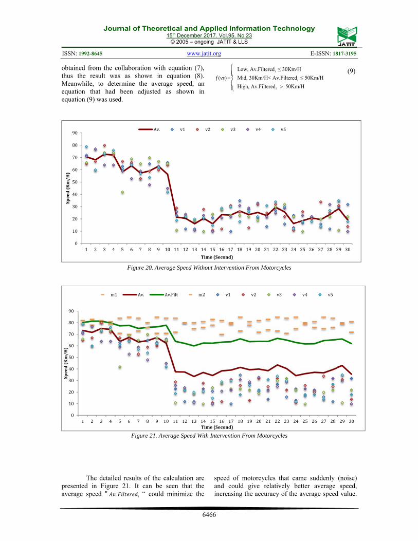
Specifically, the calculation of the vehicle speed can be stated as equation (4). The results of the vehicle speed recording are presented in Figure 20 and Figure 21. In the condition shown in Figure 21, it tends to be easier to measure the average speed. The data in those figures show the speed in the first 30 seconds on the road in Dago area. It can be seen that the car speed (m1-m5) represented by points is read by the system as different levels of speed. It is due to the domination of four-wheeled vehicles on the road (v1, v2, v3, v4, v5). This commonly happens on highways on which only four-wheeled vehicles are allowed to pass. The calculation of the average speed may use equation (4).

A problem occurred when a two-wheeled vehicle (m1, m2) suddenly appeared in a fairly high speed between cars (v1, v2, v3, v4, v5) when the traffic was in a heavy condition. This certainly would cause an error in reading the actual average speed (Av). In that condition, the speed of cars tended to be low, but suddenly a motorcycle passeds between cars in a speed above the average. This condition is shown in Figure 21. As shown in the picture, the motorcycles (m1, m2) had speed above the average speed of cars (v1-v5). To anticipate the motorcycles’ speed, we used the standard deviation equation (equation (7)), with which the sudden speed of motorcycle in heavy traffic can be minimized.

(a) The position of frame of vehicles ‘A’ and ‘B’ at minute

x

(b) The position of frame at minute x+

(c) The determination of the position of rectangle ‘A’

based on absolute ‘θ’ below 300

(d) The determination of the position of rectangle ‘B’ based

on absolute ‘θ’ below 300

Figure 19. The process of determining the next vehicle candidate (represented by a rectangle) based on the

absolute degree of slope ‘θ’ below 300

. , , , … , (7)

The calculation of the standard deviation

was used as the basis for calculating the actual average speed “ . “. The “ . “

value was used as the reference for the actual average speed.

. .

(8) As a result, instead of using the average

speed ( . ), equation (4) used the equation




6466

obtained from the collaboration with equation (7), thus the result was as shown in equation (8). Meanwhile, to determine the average speed, an equation that had been adjusted as shown in equation (9) was used.

f (vs)

Low, Av.Filteredi ≤ 30Km/H

Mid, 30Km/H< Av.Filteredi ≤ 50Km/H

High, Av.Filteredi 50Km/H

(9)

Figure 20. Average Speed Without Intervention From Motorcycles

Figure 21. Average Speed With Intervention From Motorcycles

The detailed results of the calculation are

presented in Figure 21. It can be seen that the average speed " . “ could minimize the

speed of motorcycles that came suddenly (noise) and could give relatively better average speed, increasing the accuracy of the average speed value.

0

10

20

30

40

50

60

70

80

90

1 2 3 4 5 6 7 8 9 10 11 12 13 14 15 16 17 18 19 20 21 22 23 24 25 26 27 28 29 30

Speed(Km/H)

Time(Second)

Av. v1 v2 v3 v4 v5

0

10

20

30

40

50

60

70

80

90

1 2 3 4 5 6 7 8 9 10 11 12 13 14 15 16 17 18 19 20 21 22 23 24 25 26 27 28 29 30

Speed(Km/H)

Time(Second)

m1 Av. Av.Filt m2 v1 v2 v3 v4 v5




6467

Figure 21 presents the data of results closer to the actual condition. The data presented in the picture show the speed in the first 30 seconds on the road in Dago area. They show the speed of the points read by the system in various levels. The dotted line to the top represents the speed of two-wheeled vehicles, while the dots to the bottom represent the speed of cars. The speed certainly must be able to interprate the average of these two lanes. With this standard deviation equation, the average speed can narrow down the motorcycle speed that is greater than the average. Thus, the reading result could be more accurate.

4.3. Traffic Congestion by Road Density and Vehicle Motion

In the last process, the information of road density and the information of the average speed of vehicles were combined. We developed fuzzy model based on Table 3 into the application. The results are shown in Figure 22. Light Status on the Road, Figure 23. Jam Status on the Road and Figure 24. Heavy Jam Status on the Road. This fuzzy model was able to sufficiently present the information on congestion and minimizing the speed of two-wheeled passing when the road is occupied by cars (Figure 23 and Figure 24).

If we take a look at Figure 23 and Figure 24, the conditions of the road appear to be the same in terms of both speed and density. However, in this

case, the density served as the factor that determined whether the condition belonged to jam or heavy-jam category. By referring to the fuzzy model developed, the decision on the road condition could be more accurate. However, in some conditions, we assumed that there was some condition of impossibility happening. This condition happens when the speed is high and the density is low, as well as when the speed is high and the density is moderate. Therefore, we did not include this condition into the Fuzzy model we developed. The three categories we developed are light, jam and heavy-jam, which are decided to facilitate the reading by the system to be disemminated to the road users. At first, we decided to have five categories of road conditions. However, we felt that this would not be effective in describing the actual road conditions due to the many definitions required.

The three categories (light, jam and heavy-jam) are sufficient for representing the conditions of the roads in Indonesia. Nevertheless, we also prepared the factual information concerning average speed and density. Hence, the road users will eventually be able to access adequate information regarding the existing road conditions.




6468

Figure 22. Light Status On The Road

Figure 23. Jam Status On The Road




6469

Figure 24. Heavy Jam Status On The Road

5. CONCLUSION AND FUTURE RESEARCH

Previous studies tended to play in “safe” traffic conditions, namely fluent traffic and bright weather. They did not touch heavy-jam traffic condition. This is normal given that light and moderate traffic conditions are easy and quick to process, and given that the system was not ready to be used for traffic complexity with heavy to jammed conditions. Here is where the system developed can be utilized. This system is expected to be able to anticipate the levels of road occupancy in varous conditions. With the right algorithm and system, the model proposed is able to read the road conditions in a real-time and accurate manner.

In this paper, we presented two novel

models in the context of congestion detection using road density and vehicle speed. Road density is about how wide is the road area occupied by vehicles, while vehicle speed is about how fast vehicles pass in a certain period. Therefore, the information on both will help define the levels of vehicle congestion on a road. According to the results of the temporary experiment conducted on an in-city road, this method was found to be fairly accurate in defining different levels of congestion, namely fluent, smooth and jammed. Furthermore, there was no general definition regarding the

measurement of the level of congestion on the road. Therefore, this method needs clear definition and measurement regarding the levels of congestion, which eventually will determine the information accuracy. A considerable attention should be paid in the initiation phase, which is of the upmost importance. In the initiation phase, an error in the reading will occur if there are two or more objects near each other along the initiation frame length passed. The system will automatically read the three objects as one whole object. Thus, it is certain that there will be an error in the counting of the number of vehicles. Nevertheless, this will not significantly affect the calculation of the vehicle speed as it is the average speed of the vehicles passing every frame that is calculated. This will involve more than one vehicle in a given period. Additionally, there is another minor problem occuring, which is the position of the camera. It must be assured that the position of the camera is free from the disturbance of the wind or trees, and the lens of the camera is mostly directed toward the road. This is intended to avoid interference from pedestrians or objects outside the road that also move, which will be read by the system as well and cause an error in the reading.




6470

REFERENCES:

[1] Istin, Codruta., Pescaru ,Dan., and Doboli ,Alex., (2011), Stochastic Model-Based Heuristics for Fast Field of View Loss Recovery in Urban Traffic Management Through Networks of Video Cameras., IEEE TRANSACTIONS ON INTELLIGENT TRANSPORTATION SYSTEMS, VOL. 12, NO. 3, SEPTEMBER 2011

[2] Sivaraman, Sayanan., Manubhai Trivedi, Mohan., (2013), Looking at Vehicles on the Road: A Survey of Vision-Based Vehicle Detection, Tracking, and Behavior Analysis., IEEE TRANSACTIONS ON INTELLIGENT TRANSPORTATION SYSTEMS, VOL. 14, NO. 4, DECEMBER 2013

[3] Yuniar, Roslyn., (2010), Pengenalan Benda di Jalan Raya dengan Metode Kalman Filter

[4] Cuevas, Erik., Zaldivar., Raul, Rojas., (2005), Kalman filter for vision tracking, Technical Report B 05-12, 2005

[5] Breitenstein, Michael., Reichlin, Fabian., Leibe, Bastian., (2011), Online Multiperson Tracking-by-Detection from a Single, Uncalibrated Camera, IEEE TRANSACTIONS ON PATTERN ANALYSIS AND MACHINE INTELLIGENCE, VOL. 33, NO. 9, SEPTEMBER 2011

[6] Li, Xu., Shu, Wei., Li, Ming-Lu., Wu, Min-You., (2008), Vehicle-based Sensor Networks for Traffic Monitoring

[7] Nanthawichit, C., Nakatsuji, T., and Suzuki, H., (2003), Application of Probe Vehicle Data for Real-Time Traffic State Estimation and Short- Term Travel Time Prediction on a Freeway, TRB 2003 Annual Meeting

[8] W.-L, Hsu., H,-Y.M., Liao, B.-S., Jeng and K.-C, Fan., (2004), Real-time traffic parameter extraction using entropy., IEE Proc.-Vis. Image Signal Process., Vol. 151, No. 3, June 2004

[9] Yoo, Hunjae., Yang, Ukil., Sohn, Kwanghoon.,(2013), Gradient-Enhancing Conversion for Illumination-Robust Lane Detection , IEEE Transactions on Intelligent Transportation Systems, Vol. 14, No. 3, September 2013

[10] Fritsch, Jannik., Kühnl, Tobias., Kummert, Franz., (2014), Monocular Road Terrain Detection by Combining Visual and Spatial Information, Transactions on Intelligent Transportation Systems, Vol. 15, No. 4, August 2014

[11] Liu, Guoliang., Wörgötter, Florentin., Markelic ́, Irene., (2013), Stochastic Lane Shape EstimationUsing Local Image

Descriptors, IEEE Transactions on Intelligent Transportation Systems, Vol. 14, No. 1, March 2013

[12] Kalman, RE.,(1960), A New Approach to Linear Filtering and Prediction Problems, Transactions of the ASME–Journal of Basic Engineering, 82 (Series D): 35-45. Copyright © 1960 by ASME

[13] Gupte, Surendra., Masoud, Osama., Martin, Robert., and P. Papanikolopoulos, Nikolaos., (2002), Detection and Classification of Vehicles., IEEE TRANSACTIONS ON INTELLIGENT TRANSPORTATION SYSTEMS, VOL. 3, NO. 1, MARCH 2002

[14] Beymer, David., McLauchlan, Philip., Coifman, Benn., and Malik, Jitendra., (1997), A Real-time Computer Vision System for Measuring Traffic Parameters, “1063-6919/97 $10.00 0 1997 IEEE

[15] Hsieh,Jun-Wei., Yu, Shih-Hao., Chen, Yung-Sheng., and Hu, Wen-Fong., (2006) “Automatic Traffic Surveillance System for Vehicle Tracking and Classification., IEEE TRANSACTIONS ON INTELLIGENT TRANSPORTATION SYSTEMS, VOL. 7, NO. 2, JUNE 2006

[16] Tran Morris, Brendan., Manubhai Trivedi, Mohan., (2008), Learning, Modeling, and Classification of Vehicle Track Patterns from Live Video, IEEE TRANSACTIONS ON INTELLIGENT TRANSPORTATION SYSTEMS, VOL. 9, NO. 3, SEPTEMBER 2008

[17] Chen, Chao., Jia, Zhanfeng., Varaiya, Pravin., (2001), Causes and Cures of Highway Congestion , IEEE Control Systems Magazine, December 2001

[18] Codruta Istin, Dan Pescaru, and Alex Doboli, ”Stochastic Model-Based Heuristics for Fast Field of View Loss Recovery in Urban Traffic Management Through Networks of Video Cameras,” IEEE TRANSACTIONS ON INTELLIGENT TRANSPORTATION SYSTEMS, VOL. 12, NO. 3, SEPTEMBER 2011

[19] Sayanan Sivaraman, and Mohan Manubhai Trivedi, “A General Active-Learning Framework for On-Road Vehicle Recognition and Tracking,” IEEE TRANSACTIONS ON INTELLIGENT TRANSPORTATION SYSTEMS, VOL. 11, NO. 2, JUNE 2010

[20] Anselm Haselhoff and Anton Kummert, ”An Evolutionary Optimized Vehicle Tracker in Collaboration with a Detection System, “Proceedings of the 12th International IEEE




6471

Conference on Intelligent Transportation Systems, St. Louis, MO,USA, October 3-7, 2009

[21] Erik Cuevas, Daniel Zaldivar, and Raul Rojas, “Kalman filter for vision tracking, “ Technical Report B 05-12, 2005

[22] Amirali Jazayeri, Hongyuan Cai, Jiang Yu Zheng, and Mihran Tuceryan, “Vehicle Detection and Tracking in Car Video Based on Motion Model,” IEEE TRANSACTIONS ON INTELLIGENT TRANSPORTATION SYSTEMS, VOL. 12, NO. 2, JUNE 2011

[23] Chyi-Yeu Lin, and Edwin Setiawan, “Object Orientation Recognition Based on SIFT and SVM by Using Stereo Camera,“ Proceedings of the 2008 IEEE International Conference on Robotics and Biomimetics Bangkok, Thailand, February 21 - 26, 2009

[24] Shunsuke Kamijo, Yasuyuki Matsushita, Katsushi Ikeuchi, and Masao Sakauchi, “Traffic Monitoring and Accident Detection at

Intersections, “IEEE TRANSACTIONS ON INTELLIGENT TRANSPORTATION SYSTEMS, VOL. 1, NO. 2, JUNE 2000

[25] Freeman, H., Shapira, R., (1975), “Determining the Minimum-Area Encasing Rectangle for an Arbitrary Closed Curved, “ Communications of the ACM, Volume 18, Number 7, July 1975

[26] https://www.youtube.com/watch?v=1Hpljc10gVM

[27] https://www.youtube.com/watch?v=w6gs10P2e1k

[28] https://www.youtube.com/watch?v=4i3yDNEpwro

[29] https://www.youtube.com/watch?v=oW6PxDl3pz8

[30] https://www.youtube.com/watch?v=llOk1SyHFc4&t=328s

Documents

Journal of Theoretical and Applied Information Technology ...informatika.stei.itb.ac.id/~rinaldi.munir/Penelitian/Makalah_JATIT... · accurate. The studies above did not describe