Journal of Public Economics 95 (2011) 1621–1634

Contents lists available at ScienceDirect

Journal of Public Economics

j ourna l homepage: www.e lsev ie r.com/ locate / jpube

Hindsight-biased evaluation of political decision makers☆

Florian Schuett a,⁎, Alexander K. Wagner b

a TILEC, CentER, Tilburg University, P.O. Box 90153, 5000 LE Tilburg, The Netherlandsb Department of Economics, University of Konstanz, Box 150, 78457 Konstanz, Germany

☆ We are grateful to Carlos Alós-Ferrer, Ben Ansell, DanDenicolò, Guido Friebel, Elisabetta Iossa, Raphaël Levy, RoPaul Seabright, Johannes Spinnewijn, Jean Tirole, Nicolastwo anonymous referees for helpful comments.We also thof the French Economic Association in Lyon, the LABSIconference in Padova, the Econometric Society Europeanparticipants at Toulouse School of Economics for their com⁎ Corresponding author. Tel.: +31 13 466 4033. Fax:

E-mail addresses: f.schuett@uvt.nl (F. Schuett), alexa(A.K. Wagner).

1 Starting with the work of Fischhoff (1975), psycholohas firmly established its robustness. For a guide to the v150 journal articles, two meta-analyses (Christensen-SGuilbault et al., 2004), and two special issues (Memory, VCognition, Vol. 25 (2007), Issue 1), see Blank et al. (2007)

0047-2727/$ – see front matter © 2011 Elsevier B.V. Aldoi:10.1016/j.jpubeco.2011.04.001

a b s t r a c t

a r t i c l e i n f o

Article history:Received 5 August 2009Received in revised form 30 November 2010Accepted 1 April 2011Available online 9 April 2011

JEL classification:D03D72D83C72D82

Keywords:Political agencyPolicy gamblesHindsight biasMemory distortions

Hindsight bias is a cognitive deficiency that leads people to overestimate ex post how predictable an eventwas. In this paper we develop a political-agency model in which voters are hindsight-biased and politiciansdiffer in ability, defined as information concerning the optimal policy. When public information is not tooaccurate, low-ability politicians sometimes gamble on suboptimal policies: in an attempt to mimic the high-ability type, who has superior private information, they go against public information and choose a policywhose expected payoff to society is negative. We model hindsight bias as a memory imperfection thatprevents voters from accessing their ex ante information about the state of the world. We show that the biascan act as a discipline device that reduces policy gambles and can therefore be welfare enhancing. Although itis well known that restrictions on information acquisition can be beneficial for a principal, our contribution isto show that a psychological bias can have such an effect.

Ariely, Pascal Courty, Vincenzosemarie Nagel, François Salanié,Treich, Heinrich Ursprung andank participants at themeetingconference in Siena, the ASSETMeeting in Milan, and seminarments.+31 13 466 3042.nder.wagner@uni-konstanz.de

gical research on hindsight biasast literature that includes overzalanski and Willham, 1991;ol. 11 (2003), Issues 4–5; Social.

l rights reserved.

© 2011 Elsevier B.V. All rights reserved.

1. Introduction

The psychology literature provides ample evidence that manypeople exhibit hindsight bias: in retrospect, they systematically over-estimate how predictable an event was.1 The bias can cause problemswhen a decision maker is evaluated after the outcome of his actions isknown, and no ex ante contract, mapping outcomes into performanceassessments, exists. Democratic elections are a prominent example ofsuch a situation. Voters typically have to make an ex post assessment of

the decisions of an incumbent politician and decide whether to confirmhim in office or replace him with a challenger. Hindsight bias is oftenthought to adversely affect the voters' decision by altering theirperception of the incumbent's responsibility (Camerer et al., 1989;Frey and Eichenberger, 1991). Because they deem observed outcomesmore predictable than they actually were, hindsight-biased voters tendto give the incumbent less credit than is due for success andmore blamethan is warranted for failure.

In this paper we argue that hindsight bias may not be altogetherdetrimental to the functioning of the political system because it canhave a disciplining effect on politicians. We present a model in whichthe incumbent politician has a tendency to engage in policy gambles:to mislead voters into thinking that he has superior privateinformation, the incumbent goes against public information andchooses a policy whose expected payoff to society is negative butwhich, in the event of success, boosts his chances of staying in office.We show that hindsight bias on the part of voters can reduce suchpolicy gambles and can therefore be welfare-enhancing.

Tomotivateour analysis, let usbriefly consider twoepisodes fromU.S.politics: the first Gulf war, and the Iran hostage crisis. The Gulf war of1991 is a well-documented example of how hindsight bias can influencethe public perception of policy choices, and arguably the outcome ofelections. President George H.W. Bush had initiated military action inresponse to the Iraqi invasion of Kuwait, an endeavor of considerablepolitical risk, and came away with what observers unanimously viewed

1622 F. Schuett, A.K. Wagner / Journal of Public Economics 95 (2011) 1621–1634

as a huge success. Opinion polls about the decision to go to war clearlybear out voters' hindsight bias:

In December 1990, respondents had split about 50/50 on aquestion asking whether they preferred sanctions or militaryaction. But when asked after the war how they had felt before thewar, those inclined to remember that they had supported militaryaction outnumbered those recalling their support for sanctions bynearly four to one. (Mueller, 1994, p. 87)

If voters considered thedecision togo towar as aneasy call in retrospect,such a beliefwould surelyhave beendetrimental to the President's hopeof winning reelection.2

The Iran hostage crisis illustrates the fact that policy gambles are animportant political accountability problem. In 1979, 66 U.S. diplomatshadbeen takenhostage in the Tehranembassy. President JimmyCarter'slow approval ratings and a slumping U.S. economy meant that thepresident was unlikely to be confirmed in office unless he somehowmanaged to resolve the crisis before the November 1980 election. Asnegotiations with Iran dragged on, Carter started to contemplate amilitary solution that most observers at the time thought impossible ortoo risky. Polls showed that only 10% of voters were in favor of usingmilitary force (Brulé, 2005), and Secretary of State Cyrus Vance resignedbecause of disagreement with Carter and his team of advisors on theissue (Houghton, 2001). In spite of the opposition, Carter decided tolaunch a high-risk military rescue operation. It became one of the best-known fiascos in the history of American military intervention.3

How does hindsight bias reduce the tendency toward policygambles? The reason why a politician may sometimes choose a policythat both he and the public expect to reduce welfare is that, if thegamble pays off, rational voters are “surprised” and make an upwardadjustment of their beliefs about the politician's ability. Hindsight-biased voters, however, think they knew all along that the policy wasgoing to work (they are not surprised), and do not give him as muchcredit. Therefore, when facing hindsight-biased voters, the politicianis less tempted to gamble on an inefficient policy in the first place.

To be more precise, in the model we develop, a politician whoseability is unknown to voters has to choose between two policies. Whilevoters and low-ability politicians obtain only an imperfect signal aboutwhichpolicy is preferable ex ante, high-ability politicians know the stateof the world with certainty. This setup creates incentives for a low-ability politician to inefficiently ignore public information concerningthe welfare-maximizing policy in an attempt to “look smart,” i.e., tomake it seemas if he had superior private information, the trademark ofhigh-ability politicians. To seewhy, considerwhat happens in the caseofrational voters, noting that a high-ability politician always chooses theright policy and thus disregards the publicly observed signal. If the low-ability politician always follows the signal, rational voters infer that anypolitician who chooses a policy that is contrary to the signal must be ofhigh ability; thus, successfully implementing an unpopular policysignals competence.

We show that if the public signal is in an intermediate range suchthat neither policy choice clearly dominates the other in terms ofexpected welfare, the equilibrium with rational voters has the low-ability politician randomizing between choosing the policy that isoptimal according to the signal and doing exactly the opposite. Thisrandomization is detrimental to welfare because policy choices do notuse all available information.

2 We discuss this example in more detail in Section 5.3 A phenomenon that arises as a special case of the policy gambles in our model is

gambling for resurrection. Downs and Rocke (1994) provide historical examples ofgambling for resurrection by policy makers. Systematic evidence is difficult to come bybecause the information needed to identify a behavior as gambling for resurrection isprivate. Hess and Orphanide's (1995) finding that U.S. presidents are more likely tostart a war in an election year when the economy is doing badly nevertheless suggeststhat such behavior is not merely anecdotal.

We assume that voters suffering from hindsight bias distort theirrecollection of the signal so as to make it consistent with the state ofthe world revealed by the policy outcome. If the signal suggested thatthe state of the world is 0, but the politician successfully enacts apolicy that reveals that the opposite is the case, then voters wronglybelieve that the signal had suggested all along that the state was 1.Therefore, with hindsight-biased voters, some of the gain inreputation that follows from an unpopular policy which turns out tobe a success is destroyed. Ex post, biased voters think that it was theobvious choice anyway. Anticipating voters' biased belief updating,the low-ability politician gambles on the inefficient policy less oftenwhen voters are hindsight biased than when they are rational. Thus,hindsight bias on the part of voters can act as a discipline device.

Another way to interpret the effect of hindsight bias is thefollowing. In our model, politicians sometimes try to improve theirreputation by going against the public signal. Hindsight bias makesvoters forget the public signal and replace it with an erroneousrecollection based on outcome knowledge. By doing so, the bias takesaway the tool of going against the public signal.

We also show that when the two policies are asymmetric withrespect to the probability of revealing the state of the world, hindsightbias may have a less benign effect. Because revelation of the state ofthe world has the potential to uncover the incumbent's lack of ability,the low type may refrain from choosing the more revealing policyeven though it is efficient. Under hindsight-biased evaluation, thepolitician does not get as much credit for success as he deserves.Compared to rational evaluation, he may be more inclined to choosethe policy that has lower expected welfare but whose outcome iscertain and does not entail the risk of uncovering him as a low type.Thus, hindsight bias can sometimes discourage efficient risk taking.

Even when the disciplining effect prevails, so that hindsight biasincreases voters' first-period welfare, an overall welfare assessmentalso has to take into account the second (i.e., post-election) period.We discuss how hindsight bias affects the selection of the second-period politician and conclude that the impact of the bias isambiguous. On the one hand, biased voters hold erroneous posteriorsabout the incumbent's ability, sometimes leading them to elect thewrong candidate. On the other hand, hindsight bias may generateoffsetting benefits in terms of inferences about the politician's type. Bychanging the low type's behavior in the first period, the bias can makeit easier for voters to distinguish low- from high-ability politicians.

Our contribution to the literature is twofold. First, our result that abehavioral bias can improve welfare adds to the behavioral-economicsliterature. It is similar in spirit to Compte and Postlewaite (2004),Bénabou and Tirole (2002) and Köszegi (2006). Those papers, however,consider how a psychological bias (namely, overconfidence) affectsintrapersonalwelfare.4 By contrast,we investigate howabias on the partof one group of agents (voters) can affect the behavior of other agents(politicians) in a way that increases the welfare of the former. We use astandard welfare measure that is unaffected by which “self” of anindividual one considers; nor does it involve belief consumption.

Second, our paper extends the literature on political agency, inparticular by going beyond the standard rational-voter assumption, assuggested by Besley (2006). Our basic model is related to the recentliterature on the dysfunctional effects of reelection concerns whichcan arise when politicians have better information than voters. Thisliterature has mainly emphasized distortions such as inefficient policyexperimentation and pandering (see, e.g., Majumdar and Mukand,2004; Maskin and Tirole, 2004; Smart and Sturm, 2006). The

4 In Compte and Postlewaite (2004), an agent's self-confidence affects his performancein a task. Information-processing biases such as repressing memories of bad performancecan improve the individual's welfare by boosting his confidence, thus helping him dobetter. Bénabou and Tirole (2002) show how overconfidence can help an individualovercome time inconsistency and thus improve his well-being (at least from an ex ante(“self zero”) perspective). Köszegi (2006) lets individuals consume their self-perception,so that an overly positive self-image can raise utility.

1623F. Schuett, A.K. Wagner / Journal of Public Economics 95 (2011) 1621–1634

inefficiency in our model consists in politicians signaling their abilityby choosing an unpopular policy.

Canes-Wrone et al. (2001) obtain both kinds of inefficient behaviorin a model where politicians try to signal their ability and the policiesavailable differ in the probability of uncertainty resolution, i.e., theprobability that the policy outcome is realized before the election. Incontrast to our model, the quality of the challenger is known at theoutset. When the challenger's quality is low, the low-ability incumbentmay choose a suboptimal policy simply because it is popular amongvoters (pandering). When the challenger's ability is high and theprobability of uncertainty resolution is sufficiently asymmetric, how-ever, the incumbent may engage in something the authors call “fakeleadership”: he acts against both popular belief and his private signal,trying to be perceived as a leader.5 In our model, inefficient policygambles (i.e., fake leadership) occur regardless of the asymmetrybetween probabilities of uncertainty resolution, although the effect ofhindsight bias depends on it.

Our results are similar to those obtained by Levy (2004) for thecase of decision makers with career concerns. The decision makers inher model display a behavior labeled “anti-herding,” i.e., they have atendency to take decisions contradicting the public prior. In Prat(2005), the agent may disregard valuable private information in anattempt to mimic the more able type. As a result, the principal may bebetter off not observing the agent's action.

The finding that less information can be better for a principal is acommon theme in setupswhere theprincipal lacks commitmentpower.It is a feature of Crémer (1995), for example, where the principal mayforego a costless monitoring technology in order to increase the agent'sincentives. Inourmodel, incentives for the low type are improveddue tovoters' distorted memories; it is their hindsight bias that destroysinformation. Although it is well known that restrictions on informationacquisition can be beneficial to the principal, our contribution is to showthat a psychological bias can have such an effect.

The remainder of the paper is organized as follows. Section 2introduces the model and defines a hindsight-biased informationstructure. Section 3 determines the equilibria under rational andhindsight-biased policy evaluation and compares their welfareproperties. Section 4 discusses our modeling of hindsight bias andoutlines the effect of the bias on selection. Finally, Section 5 concludes.All proofs are relegated to the Appendix.

2. Model

We consider a simple two-period political agency model. In eachperiod, the state of theworldω canbe either 0or 1. Politicians andvotersreceive an imperfect public signal σ∈{σ0,σ1} about the state of theworld. Letν∈{ν0,ν1} denote theprobability that the state of theworld is1 conditional on signalσ. That is, ν0≡Pr[ω=1|σ0] and ν1≡Pr[ω=1|σ1].There are two possible policies (or actions) a∈{a0,a1} from which thedecision maker can choose. The actions can produce different policyoutcomes y∈{0,κ,1} (defined as the payoff to voters), which depend onthe state of the world. Policy a1 delivers a payoff of 1 if ω=1, and 0 ifω=0. Thus, the outcome associated with a1 is always contingent on ω.The outcome associated with policy a0 is contingent on ω only withprobability p, in which case it delivers a payoff of 1 if ω=0, and 0 ifω=1. With probability 1−p, policy a0 delivers a payoff of κ,independent of ω. We assume 0bκb1 so that a1 yields a higher payoffthan a0 if and only if ω=1.

A politician can be of high or low ability and knows his own typeθ∈{θH,θL}. The prior probability λ∈(0,1) that the incumbent is of

5 Canes-Wrone et al. (2001) distinguish fake leadership from true leadership, thelatter being defined as a high-ability incumbent ignoring public information andfollowing his superior private signal, a behavior that is in the public interest.

high ability is common knowledge. High ability is defined as aninformational advantage over voters as to the welfare-maximizingpolicy. While a low-ability politician only learns the signal (σ), a high-ability politician also learns the state of the world (ω).

Our assumption that voters obtain an informative signal about thestate of the world, just as politicians do, and that the signal coincideswith that of low-ability politicians, reflects the idea that voters areexposed to a certain amount of policy-relevant public information(e.g., from the media). On average, politicians still have “expertise,”i.e., they are more likely to have correct information concerning theunderlying state of the world than voters.

We impose the following assumption on the signal:

Assumption 1. 0bν0b1/2bν1b1.

This assumption ensures that the public signal is informative butimperfect: while it does not reveal the state of the world withcertainty, the likelihood that the state is ω after signal σω is greaterthan the likelihood that the state is 1−ω. In other words, the signal ismore likely to be correct than incorrect.

In order tomodel hindsight bias, we introduce a distinction betweenthe original signal σ received by all players before the politician choosesan action, and the recollection σ̂ of the original signal that voters havewhen deciding who to vote for. While rational voters always correctlyrecall the signal (σ̂ = σ), hindsight-biased voters' recollection some-times differs from the original signal, as we outline below.

2.1. Timing

The game is played in two periods (interpreted as terms in office).Period 1 is divided into four stages; see Fig. 1. At t=0, nature drawsthe incumbent's type θ, the state of the world ω, and the public signalσ. All types of incumbents and voters observe σ but only type-θHincumbents learn ω. At t=1, the incumbent decides which policy toimplement. At t=2, the outcome of the policy is realized and learnedby all players. At t=3, the election stage of the game, voters choosebetween the incumbent and a challenger. The electorate's perceptionof the challenger (i.e., the probability that the challenger is of highability) is λc, which is randomly drawn from a distribution on [0,1].The perception of the incumbent's ability depends on the recollectionσ̂ that voters have of the original signal σ at this stage. In the secondperiod, following a draw of ω and σ, the appointed politician takes anaction. After that, the second-period outcome is realized and publiclyobserved. At this point, the game ends.

2.2. Politicians and voters

The voters' task is to decide whether to reelect or replace theincumbent. Their strategy consists of a probability distribution overthe actions “reelect the incumbent” and “elect the challenger” for eachpossible combination of recalled signal, action, outcome, andperceived ability of the challenger. The voters' payoff equals theexpected social welfare.

The politician's preferences are given by

u = ϕW + 1−ϕð Þ Pr reelection½ �;

where W is current-period social welfare.6 The parameter ϕ∈(0,1)measures the politician's relative concern for welfare and reelection.We assume that it satisfies the following assumption:

6 The assumption that all types of politician care about social welfare, as well asholding office, can be justified, for example, by the fact that politicians are drawn fromthe population of voters. Thus, they can be expected to consume the same goods as therest of the electorate. This formulation follows authors such as Rogoff (1990),Harrington (1993), Canes-Wrone et al. (2001) and Majumdar and Mukand (2004).

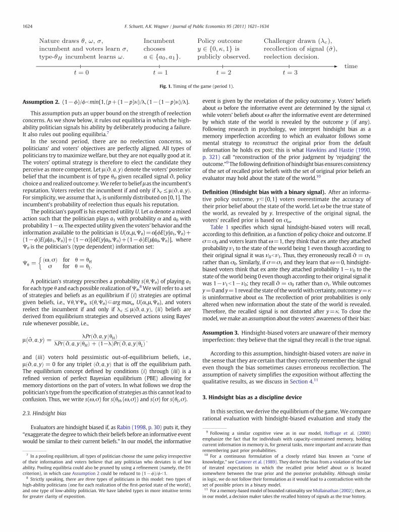
Fig. 1. Timing of the game (period 1).

9 Following a similar cognitive view as in our model, Hoffrage et al. (2000)emphasize the fact that for individuals with capacity-constrained memory, holdingcurrent information in memory is, for general tasks, more important and accurate than

1624 F. Schuett, A.K. Wagner / Journal of Public Economics 95 (2011) 1621–1634

Assumption 2. (1−ϕ)/ϕbmin{1,(p+(1−p)κ)/λ, (1−(1−p)κ)/λ}.

This assumption puts an upper bound on the strength of reelectionconcerns. As we show below, it rules out equilibria in which the high-ability politician signals his ability by deliberately producing a failure.It also rules out pooling equilibria.7

In the second period, there are no reelection concerns, sopoliticians' and voters' objectives are perfectly aligned. All types ofpoliticians try to maximize welfare, but they are not equally good at it.The voters' optimal strategy is therefore to elect the candidate theyperceive as more competent. Let μ σ̂; a; yð Þ denote the voters' posteriorbelief that the incumbent is of type θH given recalled signal σ̂, policychoice a and realized outcome y.We refer to belief μ as the incumbent'sreputation. Voters reelect the incumbent if and only if λc ≤ μ σ̂; a; yð Þ.For simplicity, we assume that λc is uniformly distributed on [0,1]. Theincumbent's probability of reelection thus equals his reputation.

The politician's payoff is his expected utility U. Let α denote a mixedaction such that the politician plays a1 with probability α and a0 withprobability 1−α. The expectedutility given thevoters' behavior and theinformation available to the politician is U(α,μ,Ψθ)=α[ϕE(y|a1,Ψθ)+(1−ϕ)E(μ|a1,Ψθ)]+(1−α)[ϕE(y|a0,Ψθ)+(1−ϕ)E(μ|a0,Ψθ)], whereΨθ is the politician's (type dependent) information set:

Ψθ =ω;σð Þ for θ = θHσ for θ = θL:

�

A politician's strategy prescribes a probability s(θ,Ψθ) of playing a1for each type θ and each possible realization ofΨθ.8Wewill refer to a setof strategies and beliefs as an equilibrium if (i) strategies are optimalgiven beliefs, i.e., ∀θ,∀Ψθ, s(θ,Ψθ)∈arg maxα U(α,μ,Ψθ), and votersreelect the incumbent if and only if λc ≤ μ σ̂; a; yð Þ, (ii) beliefs arederived from equilibrium strategies and observed actions using Bayes'rule whenever possible, i.e.,

μ σ̂; a; y� �

=λPr σ̂; a; y jθHð Þ

λPr σ̂; a; y jθHð Þ + 1−λð ÞPr σ̂; a; y jθLð Þ ;

and (iii) voters hold pessimistic out-of-equilibrium beliefs, i.e.,μ σ̂; a; yð Þ = 0 for any triplet σ̂; a; yð Þ that is off the equilibrium path.The equilibrium concept defined by conditions (i) through (iii) is arefined version of perfect Bayesian equilibrium (PBE) allowing formemory distortions on the part of voters. In what follows we drop thepolitician's type from the specification of strategies as this cannot lead toconfusion. Thus, we write s(ω,σ) for s(θH, (ω,σ)) and s(σ) for s(θL,σ).

2.3. Hindsight bias

Evaluators are hindsight biased if, as Rabin (1998, p. 30) puts it, they“exaggerate the degree towhich their beliefs before an informative eventwould be similar to their current beliefs.” In our model, the informative

7 In a pooling equilibrium, all types of politician choose the same policy irrespectiveof their information and voters believe that any politician who deviates is of lowability. Pooling equilibria could also be pruned by using a refinement (namely, the D1criterion), in which case Assumption 2 could be reduced to (1−ϕ)/ϕb1.

8 Strictly speaking, there are three types of politicians in this model: two types ofhigh-ability politicians (one for each realization of the first-period state of the world),and one type of low-ability politician. We have labeled types in more intuitive termsfor greater clarity of exposition.

event is given by the revelation of the policy outcome y. Voters' beliefsabout ω before the informative event are determined by the signal σ,while voters' beliefs aboutω after the informative event are determinedby which state of the world is revealed by the outcome y (if any).Following research in psychology, we interpret hindsight bias as amemory imperfection according to which an evaluator follows somemental strategy to reconstruct the original prior from the defaultinformation he holds ex post; this is what Hawkins and Hastie (1990,p. 321) call “reconstruction of the prior judgment by ‘rejudging’ theoutcome.”9 The followingdefinitionofhindsight bias ensures consistencyof the set of recalled prior beliefs with the set of original prior beliefs anevaluator may hold about the state of the world.10

Definition (Hindsight bias with a binary signal). After an informa-tive policy outcome, y∈ {0,1} voters overestimate the accuracy oftheir prior belief about the state of the world. Letω be the true state ofthe world, as revealed by y. Irrespective of the original signal, thevoters' recalled prior is based on σω.

Table 1 specifies which signal hindsight-biased voters will recall,according to this definition, as a function of policy choice and outcome. Ifσ=σ0 and voters learn thatω=1, they think that ex ante they attachedprobability ν1 to the state of the world being 1 even though according totheir original signal it was ν0bν1. Thus, they erroneously recall σ̂ = σ1

rather than σ0. Similarly, if σ=σ1 and they learn that ω=0, hindsight-biased voters think that ex ante they attached probability 1−ν0 to thestate of theworld being 0 even though according to their original signal itwas 1−ν1b1−ν0; they recall σ̂ = σ0 rather than σ1. While outcomesy=0andy=1reveal the stateof theworldwith certainty, outcomey=κis uninformative about ω. The recollection of prior probabilities is onlyaltered when new information about the state of the world is revealed.Therefore, the recalled signal is not distorted after y=κ. To close themodel,wemake an assumption about the voters' awareness of their bias:

Assumption 3. Hindsight-biased voters are unaware of their memoryimperfection: they believe that the signal they recall is the true signal.

According to this assumption, hindsight-biased voters are naive inthe sense that they are certain that they correctly remember the signaleven though the bias sometimes causes erroneous recollection. Theassumption of naivety simplifies the exposition without affecting thequalitative results, as we discuss in Section 4.11

3. Hindsight bias as a discipline device

In this section, we derive the equilibrium of the game.We comparerational evaluation with hindsight-biased evaluation and study the

remembering past prior probabilities.10 For a continuous formulation of a closely related bias known as “curse ofknowledge,” see Camerer et al. (1989). They derive the bias from a violation of the lawof iterated expectations in which the recalled prior belief about ω is locatedsomewhere between the true prior and the posterior probability. Although similarin logic, we do not follow their formulation as it would lead to a contradiction with theset of possible priors in a binary model.11 For a memory-basedmodel of bounded rationality seeMullainathan (2002); there, asin our model, a decision maker takes the recalled history of signals as the true history.

Table 1Biased recollection σ̂ of original signal σ.

Outcome Policy choice

a0 a1

y=0 σ1 σ0

y=κ σ –

y=1 σ0 σ1

12 It would be an abuse of language to speak of a separating equilibrium because themodel has three types of politicians; see footnote 8. The two high-ability types playpure strategies corresponding to the state of nature. Hence, whatever the low type'sstrategy, the equilibrium is always partially pooling.

1625F. Schuett, A.K. Wagner / Journal of Public Economics 95 (2011) 1621–1634

effect of the bias on first-period welfare. As a benchmark, we look atthe welfare-maximizing policy choice for the politician. The high-ability politician should always choose the policy corresponding to thestate of the world. The low-ability politician should choose policy a0 ifand only if p(1−ν)+(1−p)κ≥ν, defining a threshold value of νgiven by

ν� ≡ p + 1−pð Þκ1 + p

ð1Þ

such that policy a0 is optimal for ν≤ν* and policy a1 is optimal for νNν*.Thus, whatever the realization of the signal and the values of ν0 and ν1,there is always a unique policy that the low-ability politician shouldchoose in order to maximize expected welfare given the availableinformation.

Turning to the analysis of equilibrium, we begin by establishing thatAssumption 2 rules out equilibria in which the high-ability politiciandoes not implement the welfare-maximizing policy.

Lemma 1. Under Assumption 2, there cannot be an equilibrium inwhich the high-ability politician deviates from the welfare-maximizingpolicy.

Lemma 1 implies that, if an equilibrium exists, it must be such thatthe high-ability politician implements the welfare-maximizing policy,that is, he chooses the policy corresponding to the state of nature.Formally, s(0,σ)=0 and s(1,σ)=1, for any σ. When reelectionconcerns are not too strong, the high-ability politician never plays astrategy that requires him to choose a socially suboptimal policy. Thereason, as shown in the proof, is that the high type always hasstronger incentives to deviate from a suboptimal to the optimal policythan the low type. Note that the result of the Lemma does not dependon whether voters are rational or hindsight-biased; as long asAssumption 2 holds it is true for any beliefs. Accordingly, supposevoters believe that type θH plays the action corresponding to the stateof the world. Under Assumption 3, voters' beliefs are then given by

μ σ̂; a;0ð Þ = 0 ∀σ̂ ; a

μ σ̂; a0;κð Þ = μ σ; a0;κð Þ = λ 1−νð Þλ 1−νð Þ + 1−λð Þ 1−s σð Þð Þ

μ σ̂; a0;1ð Þ = λλ + 1−λð Þ 1−s σ̂

� �� �μ σ̂; a1;1ð Þ = λ

λ + 1−λð Þs σ̂ð Þ :

ð2Þ

Note that these expressions depend on the voters' recalled signal σ̂,which does not always coincide with the original signal σ underhindsight-biased evaluation (except when y=κ, in which case σ isalways correctly remembered). A low-ability politician's expected payofffrom a0 is then

ϕ 1−pð Þκ + p 1−νð Þ½ � + 1−ϕð Þ 1−pð Þμ σ̂; a0;κð Þ + p 1−νð Þμ σ̂; a0;1ð Þ½ �;ð3Þ

while from a1 it is

ϕν + 1−ϕð Þνμ σ̂; a1;1ð Þ: ð4Þ

Wewill categorize equilibria according to the low type's equilibriumstrategy: when s(σ)=0 or s(σ)=1, we speak of a pure-strategyequilibrium, while for 0bs(σ)b1 (the low type randomizes between a0and a1) we speak of a mixed-strategy equilibrium.12

3.1. Equilibrium with rational voters

Rational voters always correctly recall the original signal, soσ̂ = σ . Using this to replace μ according to Eq. (2) in expressions (3)and (4), the low-ability politician's payoff from action a0 becomes

ϕ 1−pð Þκ + p 1−νð Þ½ � + 1−ϕð Þ 1−pð Þλ 1−νð Þλ 1−νð Þ + 1−λð Þ 1−s σð Þð Þ +

p 1−νð Þλλ + 1−λð Þ 1−s σð Þð Þ

� �;

ð5Þwhile his payoff from a1 becomes

ϕν + 1−ϕð Þ νλλ + 1−λð Þs σð Þ : ð6Þ

Because thepolitician cares abouthis reputation aswell aswelfare, hisincentives are not perfectly aligned with those of voters. The followinglemma describes the equilibrium of the resulting game with rationalevaluation, for which sR(σ) denotes the low type's equilibrium strategy.

Lemma 2. Suppose voters are rational. There exists a uniqueequilibrium characterized by thresholds νR and νR, such that the high-ability politician chooses a0 when ω=0 and a1 when ω=1, while forν≤ νR the low-ability politician always plays a0 (sR(σ)=0), for ν≥ νR

he always plays a1 (sR(σ)=1), and for νR b ν b νR he randomizesbetween a0 and a1: sR(σ)=SR(ν) where SR(ν)∈(0,1) is increasing in ν.

In the unique equilibrium, the high-ability politician always choosesthe socially optimal policy. The low-ability politician's equilibriumbehavior depends on the probability that ω=1, given by ν. When ν issmall, we are in a pure-strategy equilibrium in which the low-abilitypolitician always chooses a0. When ν is large, we are in a pure-strategyequilibrium inwhichhealways chooses a1.Whenν is in an intermediaterange, we are in a mixed-strategy equilibrium in which he randomizesand chooses each action with probability SR(ν), obtained by equatingEqs. (5) and (6).

Note that Lemma 2 describes the equilibrium for both the σ0 and theσ1 subgame. For example, suppose ν0 b νR b ν1 b νR. Then, sR(σ0)=0and 0bsR(σ1)b1, i.e., the low type plays a0 with certainty after receivingsignal σ0, and randomizes after receiving signal σ1. Together withAssumption 1, Lemma 2 implies that sR(σ0) ≤ sR(σ1), i.e., the low-abilitypolitician is more likely to play a1 after σ1 than after σ0. It followsimmediately from the fact that there canbe amixed-strategy equilibriumthat the low type's behavior exhibits inefficiencies, as optimality requiresthe lowtype to follow the cutoff rule of playinga0 if andonly ifν ≤ ν*, anda1 otherwise (formally, νR = νR = ν�). The following propositionmakes the nature of the inefficiencies more precise.

Proposition 1. The equilibrium with rational voters involves ineffi-cient behavior by the low-ability politician for some part of the signalspace: νR N ν�, and νR bν� iff λbλ, where

λ≡1−ν� 1−ν�ð Þ−

ffiffiffiffiffiffiffiffiffiffiffiffiffiffiffiffiffiffiffiffiffiffiffiffiffiffiffiffiffiffiffiffiffiffiffiffiffiffiffiffiffiffiffiffiffiffiffiffiffiffiffiffiffiffiffiffiffiffiffiffiffiffiffiffiffiffiffiffiffiffiffi1−ν� 1−ν�ð Þð Þ2−4 ν�ð Þ2 1−ν�ð Þp

q2ν� 1−ν�ð Þp : ð7Þ

As p→1, λ→1.

Proposition 1 tells us that there is always a range of ν for which thelow-ability politician plays a0 too often (i.e., he sometimes chooses a0

1626 F. Schuett, A.K. Wagner / Journal of Public Economics 95 (2011) 1621–1634

even though a1 is optimal);moreover, if λ is not too large, there is also arange of ν for which the low-ability politician plays a1 too often. Theresult is illustrated in Fig. 2 for the casewhereλbλ and thusνR b ν� b νR.In this case, inefficiencies arise for all values of ν between νR and νR.

The basic intuition is that, because the high-ability politiciandisregards the public signal and follows his superior private informa-tion, deviating from the policy choice that the public believes to beoptimal can signal competence. While producing a failure (y=0)always leads to a reputation of zero, producing a success (y=1) hasasymmetric effects on the politician's reputation depending on howlikely the voters perceive a success as coming from a high type. Whenthere is a policy that the low type is not supposed to choose inequilibrium, voters believe that anyone who successfully implementsthis policy must be of the high type. This creates incentives for the low-ability politician to ignore the information provided by the public signaland choose the opposite of what voters believe to be optimal.

To better understand the result, it is instructive to consider twospecial cases: p=0and p=1.When p=1, the game is symmetric in thesense that both actions reveal the state of the world with probability 1.For values of ν that are in an intermediate range such that neither policyis clearly better than the other in terms of welfare, it cannot be anequilibrium for the low type to always choose the optimal policy.Suppose it were. Then, the low type could fool voters into thinking he isof the high type by successfully implementing the other policy, whichhas about equal probability of being successful but a much strongereffect on reputation. Neither can it be an equilibrium to always choosethe suboptimal policy, since then the politician could improve bothcomponents of his utility (welfare and reputation) by deviating to theoptimal policy. Thus, for ν close to 1/2, the only possible equilibriumhasthe low-ability politician randomizing between policies: sometimes hefollows the signal and chooses the efficient policy, and sometimes hegoes against the signal and gambles on the inefficient policy. Formally,with p=1 the cutoff values characterizing the low type's strategy aresuch that 0bνR = 1−νR b 1= 2 = ν�.

On the other hand, when p=0, the game is strongly asymmetric inthat action a0 never reveals the state of the world whereas a1 alwaysdoes. For large values ofν, the above argument still applies qualitatively:when a1 is better than a0 in terms of expected welfare, but not by toomuch, the equilibrium is in mixed strategies; the low type plays a0 toooften (i.e., νR N ν�). For lower values of ν, however, the low-abilitypolitician's decision problem changes, as he can now insure himselfagainst failure and the associated loss of reputation by playing a0. This isparticularly attractive when his initial reputation λ is high (λ N λ), sothat in the absence of new information he stands a good chance of beingreelected. He will then refrain from gambling on a1 for all ν b ν*, andeven choose a0with probability 1 for somevalues of ν N ν* (i.e., νR N ν�).

Fig. 2. The equilibrium strategy for type θL with rational voters.

By contrast, when λ is low (λ b λ), we have a situation that can beinterpreted as the incumbent being “behind in thepolls.” In that case, hischances of reelection are small unless he manages to change voters'opinion, which requires a political success. Thus, the low-abilitypolitician sometimes gambles on the more revealing policy a1 which,given νbν*, has negative expected social value but gives him a betterchance of being reelected (i.e., νR b ν�).

3.2. Equilibrium with hindsight biased voters

In solving for the equilibrium of the game with hindsight-biasedvoters, we assume that politicians anticipate voters' bias and that voterscorrectly predict the politician's equilibrium strategy. Thus, for eachrealization of the signal, voters know theprobability that the equilibriumstrategy assigns to the low-ability politician playing a1. To calculate theirposterior beliefs, however, voters use the probability that corresponds tothe signal they recall. Because of hindsight bias, the signal voters recallmay differ from the original signal, so their posterior beliefs can bewrong.

We now have to examine the subgames corresponding to the twosignals separately. Consider a low-ability politician pondering hispolicy choice after receiving signal σ=σ0. He knows that if he choosespolicy a0 and fails (y=0) or chooses a1 and succeeds (y=1), voterswill wrongly believe they “knew all along” that the state of the worldwas ω=1, i.e., their recalled signal will be σ̂ = σ1. When formingtheir posterior about the incumbent, they will think that the low-ability politician's equilibrium strategy assigned probability sB(σ1) toplaying a1. The politician's expected payoff from playing a0 isunaffected because μ(σ0,a0,0)=μ(σ1,a0,0)=0;13 it is still given byEq. (5). His payoff from a1, however, becomes

ϕν0 + 1−ϕð Þ ν0μ σ1; a1;1ð Þ + 1−ν0ð Þμ σ0; a1;0ð Þ½ �

= ϕν0 + 1−ϕð Þ ν0λλ + 1−λð ÞsB σ1ð Þ : ð8Þ

Similarly, consider the politician's decision problem when σ=σ1. Ifhe chooses policy a0 and succeeds (y=1)or chooses a1 and fails (y=0),voters' recalled signal will be σ̂ = σ0. When forming their posterior,they will think that the politician's strategy assigned probability sB(σ0)to playing a1. The politician's payoff from a1 is unaffected (becauseμ(σ1,a1,0)=μ(σ0,a1,0)=0) and thus given by Eq. (6). His payofffrom a0, however, becomes

ϕ p 1−ν1ð Þ + 1−pð Þκ½ � + 1−ϕð Þ½p ν1μ σ1; a0;0ð Þ + 1−ν1ð Þμ σ0; a0;1ð Þð Þ+ 1−pð Þμ σ1; a0; κð Þ� = ϕ p 1−ν1ð Þ + 1−pð Þκ½ �

+ 1−ϕð Þ p 1−ν1ð Þλλ + 1−λð Þ 1−sB σ0ð Þ� � +

1−pð Þλ 1−ν1ð Þλ 1−ν1ð Þ + 1−λð Þ 1−sB σ1ð Þ� �

" #:

ð9Þ

Expressions (8) and (9) reveal the key difference between rationaland hindsight-biased evaluation: with hindsight-biased voters, thepolitician's strategy in the σ0 subgame depends on his strategy in theσ1 subgame, and vice versa. 14 The following lemma characterizes the

13 This is partly due to the assumption of pessimistic out-of-equilibrium beliefs. Theassumption is generally not crucial though. The only case where pessimistic beliefsmatter is when s(σ1)=1 and s(σ0)b1. Without the pessimistic belief assumptionpinning down out-of-equilibrium beliefs, μ(σ1,a0,0) could be strictly positive in thatcase. Hindsight bias would then increase the incumbent's reputation in the case offailure. Such a result is counter-intuitive: we would expect hindsight bias to leadvoters to second-guess politicians' decisions and give more blame than is warranted,rather than the opposite. Any intuitive setup for hindsight bias requires out-of-equilibrium beliefs to be pessimistic.14 This is true except when p=0. In that case, the term that depends on s(σ0) inEq. (9) disappears, and sB(σ1)=sR(σ0).

Fig. 3. Equilibrium with hindsight-biased voters.

1627F. Schuett, A.K. Wagner / Journal of Public Economics 95 (2011) 1621–1634

resulting equilibriumwith hindsight-biased evaluation, for which sB(σ)denotes the low type's equilibrium strategy.

Lemma 3. Suppose voters are hindsight biased. There exists a uniqueequilibrium characterized by four thresholds, ν0

B , νB1, ν

R, and νR, suchthat the high-ability politician chooses a0 when ω=0 and a1 whenω=1, while

(i). in the σ0 subgame, for ν0 ≤ ν0B the low-ability politician

always chooses a0 (sB(σ0)=0), for ν0 ≥ νR he always choosesa1 (sB(σ0)=1), and for ν0

B b ν0 b νR he randomizes between a0and a1: sB(σ0)=S0

B(ν0,ν1) where S0B(ν0,ν1)∈(0,1) increases

with ν0 and decreases with ν1;(ii). in the σ1 subgame, for ν1 ≤ νR the low-ability politician

always chooses a0 (sB(σ1)=0), for ν1 ≥ νB1 he always chooses

a1 (sB(σ1)=1), and for νR b ν1 b νB1 he randomizes between a0

and a1: sB(σ1)=S1B(ν0,ν1) where S1

B(ν0,ν1)∈(0,1) decreaseswith ν0 and increases with ν1.

Even under hindsight-biased evaluation, the high type follows hisinformation and chooses the welfare-maximizing policy.15 Moreover,the low type's equilibrium strategy again depends on ν. In contrast tothe equilibrium under rational evaluation, there are now two sets ofthresholds, one for each subgame. In addition, both the thresholds andthe mixing probabilities in each subgame now depend on both ν0 andν1, as shown in Fig. 3. Thefigure plots ν0 on the horizontal axis andν1 onthe vertical axis, and shows the low type's equilibrium strategy sB(σ) ineach of the two subgames as a function of ν0 and ν1. The shaded trianglebelow the 45-degree line represents values such that ν0Nν1, which areruled out by Assumption 1. Fixing ν1, it remains true that for low levelsof ν0, we have a pure-strategy equilibrium in which the low type playsa0, for high levels of ν0, we have a pure-strategy equilibrium in whichthe low type plays a1, and for intermediate values, we have a mixed-strategy equilibrium. However, while in the case of rational evaluation,the equilibrium in theσ0 subgame, say, is pinned downbyν0 only, in thecase of hindsight-biased evaluation, it also depends on ν1. Fixing ν0, thelow type's equilibrium probability of playing a1 decreases with ν1.

An important observation that is apparent from Fig. 3 is that,whatever ν0 and ν1, we always have sB(σ0)≤sB(σ1). As we show inthe proof of Lemma 3, this result follows from a consistency argument.Under Assumption 1, ω=1 is more likely after σ1 than after σ0, andtherefore the expected welfare from a1 is higher after σ1 as well. Evenwith hindsight-biased voters, in equilibrium it cannot be the case thata1 is playedmore often after σ0 than after σ1. Having characterized theequilibrium under hindsight biased evaluation, we now compare thelow-ability politician's behavior to that under rational evaluation.

Proposition 2. Under hindsight-biased evaluation, the low-abilitypolitician plays a1 less often after σ0 and more often after σ1 than hedoes under rational evaluation: sB(σ0)≤ sR(σ0) and sB(σ1)≥sR(σ1).

That is, hindsight bias increases the probability that the low-abilitypolitician plays the action that—according to the signal—corresponds tothe more likely state of the world: a0 after σ0, and a1 after σ1. Theconsistency argument mentioned above is crucial for this result. Itimplies that a politicianwho successfully enacts policy a1 after signal σ0

or policy a0 after signal σ1 will get less credit than he deserves. Votersconsider the success as more predictable than it was, and thereforeoverestimate the probability that a low type would have chosen thepolicy. For example, when the original signal is σ0 but the politiciansuccessfully implements policy a1, voters wrongly believe that the

15 This means there are no adverse effects of hindsight bias on what Canes-Wrone etal. (2001) call “true leadership.” That is, a scenario in which the high-ability politicianno longer follows his private signal when voters are hindsight biased whereas he doeswhen they are rational cannot happen. It can be shown that this result does notdepend on Assumption 2 but holds more generally as long as the high-ability politicianhas perfect information.

probability of the low type playing a1 was sB(σ1) instead of sB(σ0).Because sB(σ1)≥ sB(σ0), they exaggerate the likelihood that theobserved event can be attributed to a low type, which reduces theiresteem for the incumbent.

Anticipating the voters' bias, a low-ability politician knows that hehas relatively little to gain from deviating to the action correspondingto the less likely state of the world, and does so less often. As thefollowing proposition shows, this is often good for voters' first-periodwelfare, but can sometimes be bad.

Proposition 3. Let κ ≡ ν0 1 + pð Þ−p1−p

and κ≡ ν1 1 + pð Þ−p1−p

:

For pN0, the effect of hindsight bias on first-period welfare is positiveif κ≤ κ≤ κ, and ambiguous otherwise. For p=0, the effect ofhindsight bias on first-period welfare is positive if κ≥κ = ν0, andnegative otherwise.

Note that limp→1κ = −∞ and limp→1κ = ∞. Thus, as p increases,the range of values of κ for which the effect of hindsight bias is positiveexpands, eventually to encompass the entire (0,1) interval. Based onthis insight, we can rephrase Proposition 3 as follows. When p is large,hindsight bias is sure to enhance first-period welfare. When p is small,the effect of hindsight bias depends on κ. If κ is in an intermediaterange, the effect of hindsight bias is positive; otherwise, its effect isambiguous. When p=0 and κbν0, hindsight bias is bad for first-period welfare; otherwise, its effect is positive.

According to Proposition 3, hindsight bias can enhance first-periodwelfare by improving the low-ability politician's discipline. Sometimes,however, it affects behavior in a way that is detrimental to welfare. Tobuild intuition forwhich of the two is going to happen, it is again helpfulto take a closer look at the two polar cases of p=0 and p=1. Whenp=1, we have ν*=1/2. Optimality requires that the low type plays a1after σ1 and a0 afterσ0.We know from Proposition 2 that hindsight biasnudges him in exactly this direction. Hence, for p=1 the bias is welfare-enhancing.16 By continuity, this also holds for some pb1.

Hindsight bias eliminates some of the policy gambles that occurunder rational evaluation. Recall that with rational voters, the reasonthat the low type sometimes chooses the inefficient policy is to

16 In fact, for p=1, hindsight bias leads the low type to choose the welfare-maximizing cutoff rule ν0

B = νB1 = ν� .

17 Reliability can be defined analogously for y=0. However, when y=0, posteriorbeliefs are zero regardless of the original signal, so reliability does not matter.

1628 F. Schuett, A.K. Wagner / Journal of Public Economics 95 (2011) 1621–1634

impress voters: when a policy is unlikely to be played by a low type(as is the case when the signal indicates that the other policy leads tohigher expected welfare), successfully enacting this policy boosts thepolitician's reputation. Rational voters are surprised that the policywas a success; they think that it must be attributed to a high typehaving superior private information and adjust their beliefs upward.Hindsight-biased voters are less easily impressed. They consider thepolicy outcome in retrospect more predictable than it actually was,and therefore think that choosing the right policy was “obvious” evenfor a low-ability politician. Put differently, hindsight-biased voterseffectively forget their prior when they learn the state of the world,which takes away the possibility of going against public beliefs.

When p=0, hindsight bias affects only the strategy in the σ0

subgame. The σ1 subgame is unaffected because voters do not learnanything after a0, so hindsight bias only changes the recollection fromσ1 to σ0 after a1 and outcome y=0. But μ(σ0,a1,0)=μ(σ1,a1,0)=0,implying sB(σ1)=sR(σ1) (the term in s(σ0) disappears from Eq. (9)when p=0). From Proposition 2, we know that hindsight biaschanges the strategy in the σ0 subgame towards a greater probabilityof playing a0. Whether this is good or bad for welfare depends on κ,which equals the expected payoff from a0 when p=0. The expectedpayoff from a1 is ν0. If κbν0, the expected payoff from a0 is smallerthan that from a1, and by increasing the frequency at which a0 isplayed, hindsight bias exacerbates inefficiencies. If κ≥ν0, playing a0 isefficient, so the bias has a positive effect.

The case p=0, κbν0 illustrates a second effect of hindsight bias,namely, that it sometimes discourages efficient risk-taking. Whenp=0, policy a1 is risky while policy a0 is safe, in the sense that thepolicy outcome after a1 depends on the state of the world whereasafter a0 it does not. Because the low-ability politician knows that withhindsight-biased voters he will get less credit than he deserves forsuccessfully enacting the risky policy a1, he plays a0 more often thanwith rational voters, independently of which policy is more efficient.

As we increase p slightly above zero, a countervailing effectappears that makes the effect of hindsight bias ambiguous. For lowvalues of κ (κbκ), the bias continues to exacerbate excessive play of a0in the σ0 subgame, but it now also affects the σ1 subgame, where itreduces excessive play of a0. For high values of κ (κNκ), playing a0 isefficient, and so the effect of the bias is the opposite: in the σ0

subgame, it reduces excessive play of a1, while in the σ1 subgame, itexacerbates it. Only for intermediate values of κ is hindsight biasunambiguously good: for κb κ b κ it nudges the low-ability politiciantoward the efficient choice in both subgames.

4. Discussion

The results in the previous section were derived under theassumption of naivety on the part of voters. In addition, the resultsfocus on the effect of hindsight bias on discipline (and thus first-periodwelfare). In this section, we discuss the implications of relaxingthe naivety assumption and the effect of hindsight bias on selection(and thus second-period welfare).

4.1. Awareness: naive versus sophisticated voters

According to Assumption 3, voters in our model are naive, i.e., expost unaware of their bias: they are certain that they correctlyremember the signal. The imperfect recollection process hindersconscious learning and implies a reduction in surprises. A naturalextension is to depart from the assumption of naivety as, for example,in Bénabou and Tirole (2002), where individuals repress informationbut know about their tendency to repress. Suppose that evaluators areaware of their possibly distorted recollection of the ex ante signal atthe voting stage, i.e., they are sophisticated. Voters will then use Bayes'rule to calculate the reliability of their recollection. The reliability of avoter's recollection is the probability that the recalled signal matches

the original signal. For example, suppose that a sophisticated voterobserves policy a1 and outcome y=1, and recalls signal σ1. He knowsthat, with some probability, the original signal was indeed σ1, butwith some probability it was actually σ0 and has been replaced by σ1

due to hindsight bias. Let rω≡Pr σ = σω jσ̂ = σω; y = 1;ωð Þ denotethe reliability of the voter's recollection given that the state of theworld has been revealed to be ω and y=1.17 Two of the voter'sposterior beliefs about the incumbent now have to be modified fromEq. (2). They are replaced by

μ σ0; a0;1ð Þ = r0λ

λ + 1−λð Þ 1−s σ0ð Þð Þ + 1−r0ð Þ λλ + 1−λð Þ 1−s σ1ð Þð Þ ;

μ σ1; a1;1ð Þ = r1λ

λ + 1−λð Þs σ1ð Þ + 1−r1ð Þ λλ + 1−λð Þs σ0ð Þ ;

all other beliefs are the same. Computing rω is straightforward, but itrequires some additional notation and is therefore relegated toAppendix B. A sophisticated voter questions his own memory. Whenhaving recollection σ̂ = σ1 after a successful policy a1, for example,the voter realizes that the low-ability politician played a1 withprobability s(σ1) if the recollection is reliable (probability r1) andwithprobability s(σ0) if the recollection is unreliable (probability 1−r1).

How does the behavior of the low-ability politician change whenhe faces sophisticated rather than naive voters? Notice that thepolitician's reputation after enacting a successful policy is a convexcombination of those with naive hindsight-biased and rational voters.Therefore, the effect of hindsight bias on his behavior is qualitativelythe same as with naive voters. Sophistication lowers the impact ofhindsight bias but does not eliminate it. The essence of the previousanalysis remains intact.

4.2. Selection and welfare

The analysis in Section 3 shows how hindsight bias affects thebehavior of the low-ability incumbent in the first period. To make ageneral statement about the impact of hindsight bias on welfare,however, we must also take into account the second period. Eventhough the absence of reelection concerns in the second periodmeansthat hindsight bias does not change behavior, the bias impactssecond-period welfare through its effect on selection: voters arealways weakly better off if a high-ability politician is in office.

The effect of hindsight bias on selection works through twochannels. The first is that voters sometimes have erroneous posteriors,so that they don't always elect the politician that is truly more able (inexpected terms); this is clearly bad for welfare. Hindsight bias blursthe difference between the twomajor elements voters initially set outto distinguish between in their evaluation, namely, skill and luck ofthe decision maker. The second is more indirect: since anticipation ofvoters' hindsight bias changes the low-ability politician's first-periodbehavior, the inferences that can be drawn from a given event are alsomodified. The welfare implications of this second effect are morecomplex. For example, hindsight bias increases the low type'sequilibrium probability of playing a0 after receiving σ0. This decreasesthe posterior probability that the incumbent is a high type afterobserving a0 and either y=1 or y=κ, while it increases the posteriorafter observing a1 and y=1. The net effect on selection can go eitherway and depends on various parameters such as the prior beliefsabout the state of the world.

Note that, even if hindsight bias is bad for selection, it can still begood for overall welfare. In particular, suppose κ bκ b κ, so that byProposition 3, hindsight bias has a disciplining effect on the low-ability politician. Then, there exists a discount factor such thathindsight bias is overall welfare-enhancing. Because voters discount

1629F. Schuett, A.K. Wagner / Journal of Public Economics 95 (2011) 1621–1634

the future, discipline is more important than selection for asufficiently low discount factor.

5. Conclusion

Wehave presented a political-agencymodel inwhich voters exhibit acognitive deficiency known as hindsight bias: after the uncertainty aboutan event is resolved, they consider the realized outcome as being moreforeseeable than it actually was. In themodel, voters have to evaluate theincumbent inorder todecidewhether to reelect himor replacehimwith achallenger. Politicians are assumed to differ in ability, where ability isdefined as the quality of their information about the welfare-maximizingpolicy. High-ability politicians are better informed than low-abilitypoliticians and voters. In this setup, low-ability politicians have incentivesto disregard public information on what the optimal policy is in order toappear to have superior private information. Thus, they sometimesgamble on inefficient policies.

We have shown that hindsight bias on the part of voters can act as adiscipline device. This is because hindsight-biased voters are less easilyimpressed by a successful gamble – they think it was the obvious choicefrom the outset, even if the available information had suggestedotherwise. Therefore, they give an incumbent who succeeds with apolicy gamble in spite of public pessimism less credit than rationalvoters who perfectly recall their prior. Anticipating this, low-abilitypoliticians are typically less likely to deviate from the welfare-maximizing policy. In some circumstances, however, the bias can alsodiscourage efficient risk taking, which is detrimental to voters' welfare.

We now return to the Gulf War anecdote brought up in theintroduction and discuss why it supports our claim that hindsight biascan affect elections. A case can bemade that hindsight bias contributed toGeorge H.W. Bush's defeat in the 1992 presidential election. WithBayesian voters, Bush's success in Iraqwouldhave shownuppositively inhis foreign-policy approval rate. But to hindsight-biased voters, theuse ofmilitary force seemed an obvious choice. While in the immediate post-war euphoria, approval for the President's foreign policy did go up, byApril of 1992 it was back to (or even slightly below) its pre-war level.18

Voters, in retrospect, did not give Bush much credit for the successfuloperation in the Gulf. Their hindsight biasmust have been detrimental tohis chances in theNovember1992election,whichhe lost toBill Clinton.19

Our analysismay be applicable to problems beyondpolitical economy.For example,much like elections, promotiondecisions in organizations donot follow rules set forth in an explicit ex ante contract. Consider a humanresourcesdepartment thathas todecidewhether topromoteanemployeefrom inside thefirm,whose actions andperformance have been observed,or to hire an outsider for the job. In a firm, there is typically a certainamount of public information concerning the way an employee issupposed to handle his task (in terms of themodel, what the right actionis), but employees may also have superior information on their specificassignment. Our model would predict that, if anticipated, hindsight biason the part of the human resources department may prevent low-abilityemployees fromdeviating to suboptimal actions in order to appear smart,but would not necessarily help in choosing the right candidate.

We close by noting that, with the benefit of hindsight, all of ourresults are, of course, obvious.

18 See Mueller (1994, Table 3); approval rates for Bush's handling of the situation inthe Middle East follow the same pattern. The gradual decline in the approval rate isconsistent with experimental evidence according to which hindsight bias increasesover time (Bryant and Brockway, 1997).19 Admittedly, there is some question as to whether the war in Iraq was an importantfactor in the voters' election decision. Although as late as September 1992, almost 70%of likely voters indeed said that the war was important (Mueller, 1994, Table 282),political scientists have come to view the election as largely decided by issues otherthan foreign policy. Notice, however, that this is not inconsistent with hindsight biashaving influenced the election. In fact, if voters thought that the decision to usemilitary force was a “no-brainer,” its favorable outcome should not have played muchof a role in their updating of the President's perceived competence, compared to other,seemingly more informative issues, such as his handling of the economy.

Appendix A. Proofs

Proof of Lemma 1. We have to consider two types of equilibria:pooling equilibria, and equilibria in which the high type plays a1−ω.

Claim 1. There cannot be a pooling equilibrium. Consider the followingsets of strategies and beliefs: (i) all types pool on a0, and voters believethat any politician who plays a1 is of type θL, i.e., μ(σ,a1,y)=0 ∀σ,y;(ii) all types pool on a1, and voters believe that any politician who playsa0 is of type θL, i.e., μ(σ,a0,y)=0 ∀σ,y. Regardless of σ, the type with thestrongest incentive to deviate from pooling on a0 is (θH,1). Playing a0procures him ϕ(1−p)κ+(1−ϕ)λ, while playing a1 would procure himϕ. Assumption 2 implies that he prefers a1. The type with the strongestincentive to deviate frompooling on a1 is (θH,0). Playing a1 procures him(1−ϕ)λ, while playing a0 would procure him ϕ[(1−p)κ+p]. Again,Assumption 2 implies that he prefers a0.

Claim 2. There cannot be an equilibrium inwhich thehigh type plays a1−ω.We showfirst that,whatever the voters' beliefs, (θH,1) has a stronger

incentive to play a1 than θL, and θL has a stronger incentive to play a1than (θH,0). The difference in expected payoffs between playing a1 anda0 for type θL is given by

ϕν + 1−ϕð Þ νμ σ; a1;1ð Þ + 1−νð Þμ σ; a1;0ð Þ½ �−ϕ p 1−νð Þ + 1−pð Þκ½ �− 1−ϕð Þ p νμ σ; a0;0ð Þ + 1−νð Þμ σ; a0;1ð Þð Þ + 1−pð Þμ σ; a0;κð ÞÞ½ �:

ð10Þ

The difference in expected payoffs between a1 and a0 for type(θH,0) is given by

1−ϕð Þμ σ; a1;0ð Þ−ϕ p + 1−pð Þκ½ �− 1−ϕð Þ pμ σ; a0;1ð Þ + 1−pð Þμ σ; a0; κð Þ½ �;ð11Þ

and for type (θH,1) by

ϕ + 1−ϕð Þμ σ; a1;1ð Þ−ϕ 1−pð Þκ− 1−ϕð Þ pμ σ; a0;0ð Þ + 1−pð Þμ σ; a0; κð Þ½ �:ð12Þ

Substracting Eq. (11) from Eq. (10), we see that θL's incentive toplay a1 is greater than (θH,0)'s if and only if ϕ(1+p)+(1−ϕ) [μ(σ,a1, 1)−μ(σ, a1, 0)+p(μ(σ, a0, 1)−μ(σ, a0, 0))]N0. SubtractingEq. (10) from Eq. (12), we see that (θH,1)'s incentive to play a1 isgreater than θL's under exactly the same condition. Since the term insquare brackets cannot be smaller than−(1+p) for any of the voters'beliefs, under Assumption 2 this condition is always satisfied. We canthus conclude that: if θL is indifferent, θH strictly prefers aω; if θL strictlyprefers a0, so does (θH,0); and if θL strictly prefers a1, so does type(θH,1). Hence, there cannot be an equilibrium where both (θH,0) and(θH,1) play a1−ω. □

Proof of Lemma 2. By Lemma 1, any equilibrium, if it exists, musthave the high-ability politician choosing the welfare-maximizingpolicy. Taking the behavior of the high type as given, we deriveconditions for pure and mixed strategy equilibria on the part of thelow-ability politician. We then show that, given the low type'sbehavior and voters' beliefs, the high-ability politician indeed finds itoptimal to follow the claimed equilibrium strategy.

Define Δ νð Þ≡ ϕ1−ϕ p 1−νð Þ + 1−pð Þκ−ν½ �. A pure-strategy equilib-

rium with s(σ)=0 requires that the low type prefers a0, given by Eq.(5), even though he could fool voters about his type by playing a1,given by Eq. (6), when evaluating both expressions at s(σ)=0. That is,

ϕ 1−pð Þκ + p 1−νð Þ½ � + 1−ϕð Þ 1−pð Þλ 1−νð Þ1−λν

+ p 1−νð Þλ� �

≥ν ϕ + 1−ϕð Þ½ �

ð13Þ

1630 F. Schuett, A.K. Wagner / Journal of Public Economics 95 (2011) 1621–1634

⇔Δ νð Þ≥ν− pλ 1−νð Þ + 1−pð Þλ 1−νð Þ1−λν

� �: ð14Þ

The left-hand side (LHS) is decreasing and the right-hand side(RHS) increasing in ν. Moreover, the LHS is positive and the RHSnegative when evaluated at ν=0. The LHS is negative and the RHSpositive at ν=1. Hence there exists a unique cutoff νR∈ 0;1ð Þ belowwhich sR(σ)=0 is an equilibrium. The cutoff value νR is defined byexpression (14) holding with equality. A necessary and sufficientcondition for a pure-strategy equilibrium where s(σ)=1 is that typeθL prefers a1 even though voters believe that he will always play a1.This condition is obtained by evaluating Eqs. (5) and (6) at s(σ)=1.That is,

ϕ 1−pð Þκ + p 1−νð Þ½ � + 1−ϕð Þ 1−pð Þ + p 1−νð Þ½ �≤ν ϕ + 1−ϕð Þλ½ �ð15Þ

⇔Δ νð Þ ≤ ν λ + pð Þ−1: ð16Þ

The LHS is decreasing and the RHS is increasing in ν. Moreover, theLHS is positive and the RHS negative when evaluated at ν=0. Hencethere exists a unique cutoff νRN0 above which sR(σ)=1 is anequilibrium. The cutoff value νR is defined by expression (16) holdingwith equality.

Uniqueness follows from Lemma 1 and the fact that νRb νR. To seethat this inequality must hold, notice that the LHS of expressions (14)and (16) coincides and is monotone decreasing in ν. At the same time,the RHS of Eq. (14) exceeds that of Eq. (16),

ν 1 + pλð Þ− pλ + 1−pð Þλ 1−νð Þ1−λν

� �Nν λ + pð Þ−1;

because the term in square brackets is smaller than 1 and 1+pλNλ+p⇔λ+(1−λ)pb1.

For values νR bν b νR the equilibrium is in mixed strategies, wheresR(σ)=SR(ν)∈(0,1). Type θL's equilibrium probability of playing a1,SR(ν), is determined by equating Eqs. (3) and (4), or

Δ νð Þ = νλλ + 1−λð ÞSR νð Þ−

1−pð Þλ 1−νð Þλ 1−νð Þ + 1−λð Þ 1−SR νð Þ� �

− pλ 1−νð Þλ + 1−λð Þð1−SR νð ÞÞ : ð17Þ

Next, we prove the claimed monotonicity property of SR(ν) byapplying the implicit function theorem.Define f ≡ LHS−RHSof Eq. (17).

We then havedSR νð Þdν

= − ∂f = ∂ν∂f = ∂SR : It is straightforward to see that

∂ f/∂SRN0 and ∂ f/∂ν b 0. Hence, dSR/dν N 0.We finally show that, given the voters' beliefs, it is indeed optimal

for the high-ability politician to choose the policy corresponding to ω.Consider first type (θH,0). He prefers a0 since

Δ 0ð Þ + 1−pð Þλ 1−νð Þλ 1−νð Þ + 1−λð Þ 1−sR σð Þ� � +

pλλ + 1−λð Þ 1−sR σð Þ� �

" #N0

ð18Þ

for any sR(σ). Now consider type (θH, 1). The condition for him toprefer a1 to a0 is

Δ 1ð Þ≤ λλ + 1−λð ÞsR σð Þ−

1−pð Þλ 1−νð Þλ 1−νð Þ + 1−λð Þ 1−sR σð Þ� � : ð19Þ

Clearly, Δ(1)b0. There are three different cases. If νbνR so thatsR(σ)=0, type (θH,1) has a strict preference for a1 because Δ 1ð Þb1−λ + pλ 1−νð Þ

1−λν: If νNνR so that sR(σ)=1, he prefers a1 because

Δ(1)bλ+p−1 is a necessary condition for the low type to play a pure

strategy with s(σ)=1; see Eq. (16). If νR bνbνR we are in a mixed

strategy equilibriumwhere sR(σ)=SR(ν). Type (θH,1) strictly prefers a1

since Δ 1ð Þ b λλ + 1−λð ÞSR νð Þ−

1−pð Þλ 1−νð Þλ 1−νð Þ + 1−λð Þ 1−SR νð Þð Þ follows

from Eq. (17). □

Proof of Proposition 1. Solving Eq. (16) for νR yields νR =ϕ p + 1−pð Þκð Þ + 1−ϕ

ϕ + 1−ϕð Þλ + p:

The numerator of this expression is larger than that of ν* (it is aconvex combination of p+(1−p)κ and 1). The denominator issmaller than that of ν* (because ϕ+(1−ϕ)λb1). Hence, ν�b νR. TheRHS of Eq. (14) is monotone decreasing in ν and becomes zero atν=ν*. The LHS is monotone increasing in ν since its derivative withrespect to ν is

1 + pλ +λ 1−λð Þ 1−pð Þ

1−λνð Þ2 N 0:

Thus, a necessary and sufficient condition for ν� N νR is that the LHSof Eq. (14) is greater than zero when evaluated at ν=ν*. That is,

ν�− p 1−ν�ð Þλ +1−pð Þλ 1−ν�ð Þ

1−λν�

� �N 0

⇔pν� 1−ν�ð Þλ2− 1−ν� 1−ν�ð Þ½ �λ + ν� N 0:

ð20Þ

The LHS of Eq. (20) is a quadratic function of λwhose minimum isattained at λ=[1−ν*(1−ν*)]/(2pν*(1−ν*)), which is greater orequal to 3/2. Therefore, the relevant condition is that λb λ defined inEq. (7). The expression under the square root is nonnegative since(1−ν*(1−ν*))2−4p(ν*)2(1−ν*)≥(1−ν*(1−ν*))2−4(ν*)2(1−ν*)=(ν*(1+ν*))2. Finally, evaluating Eq. (7) at p=1 (which implies ν*=1/2),we have λ = 1. □

Proof of Lemma 3. By Lemma 1, any equilibrium, if it exists, musthave the high-ability politician choosing the welfare-maximizingpolicy. We thus look for an equilibrium in which this is the case andderive conditions for pure andmixed strategies on the part of the low-ability politician. We then show that, given the low type's behaviorand voters' beliefs, the high-ability politician indeed finds it optimal tofollow the equilibrium strategy.

Pure strategies. Consider first the σ0 subgame. A necessary andsufficient condition for a pure-strategy equilibrium with sB(σ0)=0 isthat type θL's payoff from playing a0, given by Eq. (5), is greater than

1631F. Schuett, A.K. Wagner / Journal of Public Economics 95 (2011) 1621–1634

his payoff from a1, given by Eq. (8), when evaluating both of theseexpressions at sB(σ0)=0. That is,

ϕ p 1−ν0ð Þ + 1−pð Þκ½ � + 1−ϕð Þ pλ 1−ν0ð Þ + 1−pð Þλ 1−ν0ð Þ1−λν0

� �≥ ϕν0

+ 1−ϕð Þ ν0λλ + 1−λð ÞsB σ1ð Þ

⇔Δ ν0ð Þ≥ ν0λλ + 1−λð ÞsB σ1ð Þ−pλ 1−ν0ð Þ− 1−pð Þλ 1−ν0ð Þ

1−λν0:

ð21Þ

The LHS is decreasing in ν0. The RHS is increasing in ν0 if sB(σ1) isdecreasing in ν0, which we will show to be the case below. Moreover,Δ(0)N0 and the RHS is negativewhen evaluated atν0=0. Therefore, fora given ν1, there exists a unique cutoff ν0

B N 0 belowwhich sB(σ0)=0 isan equilibrium. (The cutoff may be greater than 1/2.)

The condition for a pure-strategy equilibrium with sB(σ0)=1 isthat type θL's payoff from a0 is smaller than his payoff from a1 whenboth are evaluated at sB(σ0)=1, that is,

ϕ p 1−ν0ð Þ + 1−pð Þκ½ � + 1−ϕð Þ p 1−ν0ð Þ + 1−p½ �≤ϕν0 + 1−ϕð Þ ν0λλ + 1−λð ÞsB σ1ð Þ

⇔Δ ν0ð Þ≤ν0λ

λ + 1−λð ÞsB σ1ð Þ + p� �

−1:

ð22Þ

Again, the LHS is decreasing and the RHS increasing in ν0 if sB(σ1) isdecreasing in ν0. Therefore, for a given ν1, there exists a unique cutoffνB0 above which sB(σ0)=1 is an equilibrium. Note that for sB(σ1)=1,

Eq. (22) is the same as the corresponding expression in the rationalcase, Eq. (16), defining νR; note also that the RHS of Eq. (22) isdecreasing in sB(σ1), implying that νB

0 must equal νR for sB(σ1)=1 andwould have to be strictly less than νR for sB(σ1)b1. Since, as we willshow below, consistency requires sB(σ0)≤sB(σ1) for any (ν0,ν1)satisfying Assumption 1, we conclude that there cannot be a valueof ν0 b νR such that sB(σ0)=1. Thiswould require that for some ν1Nν0,sB(σ1)b1, a contradiction. Hence, νB

0 = νR.Now consider the σ1 subgame. A necessary and sufficient

condition for a pure-strategy equilibrium with sB(σ1)=0 is thattype θL's payoff from playing a0, given by Eq. (9), is greater than hispayoff from a1, given by Eq. (6), when evaluating both of theseexpressions at sB(σ1)=0. That is,

ϕ p 1−ν1ð Þ + 1−pð Þκ½ � + 1−ϕð Þ pλ 1−ν1ð Þλ + 1−λð Þ 1−sB σ0ð Þ� � +

1−pð Þλ 1−ν1ð Þ1−λν1

" #

≥ϕν1 + 1−ϕð Þν1

⇔Δ ν1ð Þ≥ν1−pλ 1−ν1ð Þ

λ + 1−λð Þ 1−sB σ0ð Þ� � +1−pð Þλ 1−ν1ð Þ

1−λν1

" #:

ð23Þ

The LHS is decreasing in ν1. The RHS is increasing in ν1 if sB(σ0) isdecreasing in ν1, which we will show to be the case below. Therefore,for a given ν0, there exists a unique cutoff ν1

B below which sB(σ1)=0is an equilibrium. (The cutoff may be smaller than 1/2.) Note that forsB(σ0)=0, Eq. (23) is the same as the corresponding expression in therational case, Eq. (14), defining νR; note also that the RHS of Eq. (23) isincreasing in sB(σ0), implying that ν1

B must equal νR for sB(σ0)=0 andwould have to be strictly greater than νR for sB(σ1)b1. Since, as wewill show below, consistency requires sB(σ0)≤sB(σ1) for any (ν0,ν1)satisfying Assumption 1, we conclude that there cannot be a valueof ν1 NνR such that sB(σ1)=0. This would require that for someν0bν1, sB(σ0)N0, a contradiction. Hence, ν1

B = νR.

The condition for a pure-strategy equilibrium with sB(σ1)=1 isthat type θL's payoff from a0 is smaller than his payoff from a1 whenboth are evaluated at sB(σ1)=1, that is,

ϕ p 1−ν1ð Þ + 1−pð Þκ½ � + 1−ϕð Þ pλ 1−ν1ð Þλ + 1−λð Þ 1−sB σ0ð Þ� � + 1−p

" #≤ϕν1 + 1−ϕð Þν1λ

⇔Δ ν1ð Þ≤ ν1λ−pλ 1−ν1ð Þ

λ + 1−λð Þ 1−sB σ0ð Þ� �− 1−pð Þ:

ð24Þ

Again, the LHS is decreasing and the RHS increasing in ν1 if sB(σ0)is decreasing in ν1. Therefore, for a given ν0, there exists a uniquecutoff νB

1 above which sB(σ1)=1 is an equilibrium. (This cutoff maynot be strictly less than 1.)

Uniqueness. Uniqueness of the equilibrium follows from the factthat (a) the RHS of Eq. (21) is greater than that of Eq. (22) for any ν0 as

1−pν0≥λ 1−ν0ð Þ p +1−p

1−λν0

� ⇔1−pν0 1 + λ 1−ν0ð Þð Þ|fflfflfflfflfflfflfflfflfflfflfflfflfflfflffl{zfflfflfflfflfflfflfflfflfflfflfflfflfflfflffl}

≤1

≥0;

implying ν0B≤ νB

0 , and (b) the RHS of Eq. (21) is greater than that of Eq.(22) for any ν1 as

ν1− 1−pð Þλ 1−ν1ð Þ1−λν1

≥ν1λ− 1−pð Þ⇔ν1≥ 1−pð Þ − 11−λν1

� ;

implying ν1B ≤ νB

1 .

Mixed strategies. In a mixed strategy equilibrium, we have sB(σ0)=S0B(ν0,ν1) and sB(σ1)=S1

B(ν0,ν1), where S0B and S1

B solve the followingsystem, obtained by equating Eq. (5) with Eq. (8), and Eq. (9) withEq. (6):

Δ ν0ð Þ = ν0λλ + 1−λð ÞSB1

− pλ 1−ν0ð Þλ + 1−λð Þ 1−SB0

� �− 1−pð Þλ 1−ν0ð Þλ 1−ν0ð Þ + 1−λð Þ 1−SB0

� �ð25Þ

Δ ν1ð Þ = ν1λλ + 1−λð ÞSB1

− pλ 1−ν1ð Þλ + 1−λð Þ 1−SB0

� �− 1−pð Þλ 1−ν1ð Þλ 1−ν1ð Þ + 1−λð Þ 1−SB1

� � :ð26Þ

To determine when there is mixing in at least one of the subgames,we need to define the thresholds ν0

B and νB1 as a function of ν1 and ν0,

respectively. Let ν̂ denote the value of ν0 that solves Eq. (21) with

equality for s(σ1)=1, i.e., Δ ν̂� �

= ν̂λ−pλ 1−ν̂� �

− 1−pð Þλ 1−ν̂� �1−λν̂

:

Similarly, let ν̃ denote the value of ν1 that solves Eq. (24) with

equality for s(σ0)=0, i.e., Δ ν̃ð Þ = ν̃λ−pλ 1−ν̃ð Þ− 1−pð Þ: Notice that,

by definition of ν0B, SB1 ν0

B;ν1� �

is the solution to Eq. (26) fixing S0B=0.

Likewise, by definition of νB1 , S

B0 ν0;ν

B1

� �is the solution to Eq. (25)

fixing S1B=1. Let V0(ν1) be defined as the solution to

Δ V0ð Þ = V0λ

λ + 1−λð ÞSB1 ν0B;ν1

� �−pλ 1−V0ð Þ− 1−pð Þλ 1−V0ð Þ1−λV0

; ð27Þ

1632 F. Schuett, A.K. Wagner / Journal of Public Economics 95 (2011) 1621–1634

and V1(ν0) as the solution to

Δ V1ð Þ = V1λ−pλ 1−V1ð Þ

λ + 1−λð Þ 1−SB0 ν0;νB1

� �� �− 1−pð Þ: ð28Þ

Then, we have

ν0B =

νR for ν1≤ νR

V0 ν1ð Þ for νR b ν1 b ν̃ν̂ for ν1 ≥ ν̃

8<:

and

νB1 =

ν̃ for ν0 ≤ ν̂V1 ν0ð Þ for ν̂ bν0 b νR

νR for ν0 ≥ νR:

8<:

Clearly, νR≤ V0 ν1ð Þ≤ ν̂ for any ν1, and ν̃≤ V1 ν0ð Þ≤ νR for any ν0.Monotonicity properties of SB. We now prove the claimed

monotonicity properties of S0B and S1B. Let

f0 ≡Δ ν0ð Þ− ν0λλ + 1−λð ÞS1

+pλ 1−ν0ð Þ

λ + 1−λð Þ 1−S0ð Þ +1−pð Þλ 1−ν0ð Þ

λ 1−ν0ð Þ + 1−λð Þ 1−S0ð Þ ;

f1 ≡Δ ν1ð Þ− ν1λλ + 1−λð ÞS1

+pλ 1−ν1ð Þ

λ + 1−λð Þ 1−S0ð Þ +1−pð Þλ 1−ν1ð Þ

λ 1−ν1ð Þ + 1−λð Þ 1−S1ð Þ :

Suppose that (S0B,S1B) is an equilibrium for some (ν0,ν1), i.e., that itsolves

f0 SB0 ; SB1 ;ν0;ν1

� �= 0

f1 SB0 ; SB1 ;ν0;ν1

� �= 0:

Totally differentiating, we have, in matrix notation,

∂f0∂S0

∂f0∂S1

∂f1∂S0

∂f1∂S1

0BBBB@

1CCCCA dS0

dS1

� =

− ∂f0∂ν0

dν0 − ∂f0∂ν1

dν1

− ∂f1∂ν0

dν0 − ∂f1∂ν1

dν1

0BBB@

1CCCA: ð29Þ

Clearly, ∂ fσ/∂Sσ′N0 for all σ and σ′, while ∂ fσ/∂νσ′b0 for all σ=σ′and ∂ fσ/∂νσ′=0 for all σ≠σ′. Let

M≡det

∂f0∂S0

∂f0∂S1

∂f1∂S0

∂f1∂S1

0BBBB@

1CCCCA =

∂f0∂S0

∂f1∂S1

− ∂f0∂S1

∂f1∂S0

:

Computation yields that MN0 if and only if

p 1−ν0ð Þλ + 1−λð Þ 1−S0ð Þð Þ|fflfflfflfflfflfflfflfflfflfflfflfflfflfflfflfflfflffl{zfflfflfflfflfflfflfflfflfflfflfflfflfflfflfflfflfflffl}2

≡A

+1−pð Þ 1−ν0ð Þ

λ 1−ν0ð Þ + 1−λð Þ 1−S0ð Þð Þ|fflfflfflfflfflfflfflfflfflfflfflfflfflfflfflfflfflfflfflfflfflfflfflfflfflffl{zfflfflfflfflfflfflfflfflfflfflfflfflfflfflfflfflfflfflfflfflfflfflfflfflfflffl}2≡B

0BBBB@

1CCCCA

⋅ν1

λ + 1−λð ÞS1ð Þ|fflfflfflfflfflfflfflfflfflfflfflfflffl{zfflfflfflfflfflfflfflfflfflfflfflfflffl}2≡C

+1−pð Þ 1−ν1ð Þ

λ 1−ν1ð Þ + 1−λð Þ 1−S1ð Þð Þ|fflfflfflfflfflfflfflfflfflfflfflfflfflfflfflfflfflfflfflfflfflfflfflfflfflffl{zfflfflfflfflfflfflfflfflfflfflfflfflfflfflfflfflfflfflfflfflfflfflfflfflfflffl}2≡D

0BBBB@

1CCCCA

Nν0

λ + 1−λð ÞS1ð Þ|fflfflfflfflfflfflfflfflfflfflfflfflffl{zfflfflfflfflfflfflfflfflfflfflfflfflffl}2≡E

⋅p 1−ν1ð Þ

λ + 1−λð Þ 1−S0ð Þð Þ|fflfflfflfflfflfflfflfflfflfflfflfflfflfflfflfflfflffl{zfflfflfflfflfflfflfflfflfflfflfflfflfflfflfflfflfflffl}2≡F:

ð30Þ

Under Assumption 1, A≥F and CNE, while B,D≥0. Therefore,MN0,and we can invert Eq. (29) to obtain

dS0dS1

� =

1M

∂f1∂S1

− ∂f0∂S1

− ∂f1∂S0

∂f0∂S0

0BBBB@

1CCCCA

− ∂f0∂ν0

dν0

− ∂f1∂ν1

dν1

0BBBB@

1CCCCA: ð31Þ

This implies

dS0dν0

=1M

∂f1∂S1

− ∂f0∂ν0

� N 0 ð32Þ

dS0dν1

=1M

− ∂f0∂S1

� − ∂f1

∂ν1

� b 0 ð33Þ

dS1dν0

=1M

− ∂f1∂S0

� − ∂f0

∂ν0

� b 0 ð34Þ

dS1dν1

=1M

∂f0∂S0

− ∂f1∂ν1

� N 0; ð35Þ

establishing the claimed monotonicity properties.Consistency. Next, we turn to the consistency condition accord-

ing to which sB(σ0) ≤ sB(σ1) for any pair (ν0,ν1). Suppose firstν0 ≤ ν0

B. Then, sB(σ0)=0. Similarly, suppose ν1 ≥ νB1 . Then, s

B(σ1)=1. In both cases consistency is trivially satisfied. Next supposeν0 N ν0

B and ν1 b νB1 , so that Eq. (25) holds with ≤ and Eq. (26) holds

with ≥. Subtracting Eq. (26) from Eq. (25), we then have, aftersimplifying,

ν1−ν0ð Þ pλλ + 1−λð Þ 1−sB σ0ð Þ� � +

λλ + 1−λð ÞsB σ1ð Þ +

ϕ1−ϕ

1 + pð Þ" #

≤ 1−pð Þλ 1−ν1ð Þλ 1−ν1ð Þ + 1−λð Þ 1−sB σ1ð Þ� �− 1−pð Þλ 1−ν0ð Þ

λ 1−ν0ð Þ + 1−λð Þ 1−sB σ0ð Þ� � :ð36Þ

The LHS is strictly positive because ν1Nν0 by Assumption 1. Thus,a necessary condition for the inequality to hold is that the RHS bestrictly positive as well. Suppose that contrary to the consistencyrequirement we have sB(σ0)NsB(σ1). This implies (1−ν1)(1−λ)

1633F. Schuett, A.K. Wagner / Journal of Public Economics 95 (2011) 1621–1634

(1− sB(σ0))b(1−ν0)(1−λ)(1− sB(σ1)). Adding λ(1−ν0)(1−ν1)to both sides of the inequality, and rearranging, we obtain

1−ν1

λ 1−ν1ð Þ + 1−λð Þ 1−sB σ1ð Þ� � b1−ν0

λ 1−ν0ð Þ + 1−λð Þ 1−sB σ0ð Þ� � ;a contradiction with the RHS of Eq. (36) being positive.

The high-ability politician. Finally, we examine the high-abilitypolitician's incentive to adhere to the prescribed equilibrium strategy.Consider type (θH,0). He prefers a0 since

ϕ p + 1−pð Þκ½ � + 1−ϕð Þ pλλ + 1−λð Þð1−sB σ0ð Þ +

1−pð Þλ 1−νð Þλ 1−νð Þ + 1−λð Þ 1−sB σ0ð Þ� �

" #N 0

for any sB(σ0). Next, consider type (θH,1). The condition for him toprefer a1 to a0 is

ϕ 1−pð Þκ + 1−ϕð Þ 1−pð Þλ 1−νð Þλ 1−νð Þ + 1−λð Þ 1−sB σ0ð Þ� � ≤ϕ

+ 1−ϕð Þ λλ + 1−λð ÞsB σ1ð Þ

⇔Δ 1ð Þ≤ λλ + 1−λð ÞsB σ1ð Þ−

1−pð Þλ 1−νð Þλ 1−νð Þ + 1−λð Þ 1−sB σ0ð Þ� � :

ð37Þ

There are several different cases. Suppose first that sB(σ0)=0. TheRHS of Eq. (37) becomes

λ

λ + 1−λð ÞsB σ1ð Þ|fflfflfflfflfflfflfflfflfflfflfflfflfflfflffl{zfflfflfflfflfflfflfflfflfflfflfflfflfflfflffl}≥λ

− 1−pð Þλ 1−νð Þ1−λν|fflfflffl{zfflfflffl}≤λ

≥0:

Now suppose that sB(σ1)=0. The RHS of Eq. (37) becomes

1− 1−pð Þλ 1−νð Þλ 1−νð Þ + 1−λð Þ 1−sB σ0ð Þð Þ≥0: Thus, if either sB(σ0) or sB(σ1)

equals zero, Eq. (37) is satisfied because Δ(1) b 0. Suppose instead thatneither equals zero, andconsider theσ0 subgame. If 0 b sB(σ0)b1, Eq. (25)must hold; if instead sB(σ0)=1, Eq. (22)must hold. Each implies Eq. (37).Now consider the σ1 subgame. If 0 b sB(σ1) b 1, Eq. (26) must hold; ifinstead sB(σ1)=1, Eq. (24)must hold. Again, each implies Eq. (37). □

Proof of Proposition 2. We know from the proof of Lemma 3 thatνR = ν1

B≤ν0B and ν B

1 ≤ν B0 = νR. Thus, if ν≤νR, then sB(σ)=sR(σ)=

0, and if ν≥νR, then sB(σ)=sR(σ)=1. For the rest of the proof, weonly have to consider values of ν in the interval νR;νR

� �.

Fig. 4. Determination of the low-type's equilibrium strategy in the σ0 subgame.

Claim 1. Suppose νR bν0 b νR. Then, sB(σ0)≤ sR(σ0) if and only ifsB(σ1)≥ sR(σ0).

When νR bν0 bνR, the rational-evaluation equilibrium in the σ0-

subgame is in mixed strategies, i.e., sR(σ0)=SR(ν0) where SR∈(0,1) isdetermined by Eq. (17); see Lemma 2. Writing out Eq. (17) for σ=σ0

and rearranging, we have

pλ 1−ν0ð Þλ + 1−λð Þ 1−s σ0ð Þð Þ +

1−pð Þλ 1−ν0ð Þλ 1−ν0ð Þ + 1−λð Þ 1−s σ0ð Þð Þ + Δ ν0ð Þ = ν0λ

λ + 1−λð Þs σ0ð Þ :

ð38Þ

The equilibrium under hindsight-biased evaluation is determinedby the following expression:

pλ 1−ν0ð Þλ + 1−λð Þ 1−s σ0ð Þð Þ +

1−pð Þλ 1−ν0ð Þλ 1−ν0ð Þ + 1−λð Þ 1−s σ0ð Þð Þ + Δ ν0ð Þe ν0λ

λ + 1−λð ÞsB σ1ð Þ :

ð39Þ

Fig. 4, which plots the left- and RHSs of expressions (38) and (39)against s(σ0), illustrates the logic of the argument that follows. The LHSof Eqs. (38) and (39) coincides and is monotone increasing in s(σ0).Under rational evaluation, the RHS, denoted RHSR in the figure, ismonotone decreasing in s(σ0). The equilibrium strategy sR

* (σ0) lies atthe intersection of the LHS with the RHSR curve. Under hindsight-biased evaluation, the RHS is constantwith respect to s(σ0); its value isobtained by evaluating RHSR at sB(σ1), yielding the horizontal linedenoted RHSB in the figure. The equilibrium strategy sB(σ0) lies at theintersection of the LHS with the RHSB curve if such an intersectionexists. If LHS≥RHSB for all s(σ0), then sB(σ0)=0. If LHS≤RHSB for alls(σ0), then sB(σ0)=1. As the figure clearly shows, the monotonicityproperties of the LHS and RHS expressions imply that the claimedrelationship must hold.

Claim 2. Suppose νR b ν1 b νR. Then, sB(σ1)≥sR(σ1) if and only ifsB(σ0)≤sR(σ1).

When νR bν1 bνR, the rational-evaluation equilibrium in the σ1-

subgame is in mixed strategies and again determined by Eq. (17).After rearranging, Eq. (17) yields, for σ=σ1,

pλ 1−ν1ð Þλ + 1−λð Þ 1−s σ1ð Þð Þ =

ν1λλ + 1−λð Þs σ1ð Þ−

1−pð Þλ 1−ν1ð Þλ 1−ν1ð Þ + 1−λð Þ 1−s σ1ð Þð Þ−Δ ν1ð Þ:

ð40Þ

The equilibrium under hindsight-biased evaluation is determinedby the following expression:

pλ 1−ν1ð Þλ + 1−λð Þ 1−sB σ0ð Þ� �e ν1λ

λ + 1−λð Þs σ1ð Þ−1−pð Þλ 1−ν1ð Þ

λ 1−ν1ð Þ + 1−λð Þ 1−s σ1ð Þð Þ−Δ ν1ð Þ:

ð41Þ

The RHS of Eqs. (40) and (41) coincides and is monotonedecreasing in s(σ1). The LHS of Eq. (40) is monotone increasing ins(σ1). The LHS of Eq. (41) is constant with respect to s(σ1); its valueis obtained by evaluating the RHS of Eq. (40) at sB(σ0). An analogousargument to the one used in the proof of Claim 1 establishes Claim 2.Combining Claims 1 and 2 with the consistency result from the proofof Lemma 3, we must have sB(σ0) ≤ sR(σ) ≤ sB(σ1), σ=σ0,σ1. Giventhat sR(σ0) ≤ sR(σ1) by Lemma 2 and Assumption 1, the only possibleordering of equilibrium strategies thus is sB(σ0) ≤ sR(σ0) ≤ sR(σ1) ≤sB(σ1). □

Proof of Proposition 3. Suppose ν0≤ν*≤ν1. Then, expected welfarein the first period is decreasing in s(σ0) and increasing in s(σ1).

1634 F. Schuett, A.K. Wagner / Journal of Public Economics 95 (2011) 1621–1634

Because by Proposition 2, sB(σ0)≤sR(σ0) and sB(σ1)≥sR(σ1), hindsightbias increases first-period welfare. From the definition of ν*,

ν0≤ν�≤ν1⇔ν0 1 + pð Þ−p

1−p= κ ≤ κ≤ ν1 1 + pð Þ−p

1−p= κ:

Now suppose ν0 b ν1 b ν�⇔κ N κ. Then, first-period welfare isdecreasing in both s(σ0) and s(σ1). If pN0, hindsight bias has a positiveeffect in the σ0 subgame but a negative effect in the σ1 subgame; theoverall effect is ambiguous. If p=0, however, the term in s(σ0) in (9)disappears, implying that sB(σ1)=sR(σ1). Hence, hindsight bias hasno effect in the σ1 subgame; its overall effect is positive. Finally,suppose ν� b ν0 b ν1⇔κ b κ. Then, first-period welfare is increasing inboth s(σ0) and s(σ1). If pN0, hindsight bias has a negative effect in theσ0 subgamebut a positive effect in theσ1 subgame; the overall effect isambiguous. If p=0, sB(σ1)=sR(σ1), so hindsight bias has no effect intheσ1 subgame; its overall effect is negative. □

Appendix B. Sophisticated voters and reliability

Denote the probability that the state of the world is 1 by π andthe probability that the signal matches the underlying state of the

world by xω≡Pr(σω|ω). Since ν0 =π 1−x1ð Þ

π 1−x1ð Þ + 1−πð Þx0 and ν1 =πx1

πx1 + 1−πð Þ 1−x0ð Þ, to be consistent with Assumption 1, x0, x1 and π

must satisfy (x0,x1,π)∈(0,1)3 and1−x0x1

bπ

1−πb

x01−x1

: We can apply

Bayes' rule to obtain

r0 =x0 λ + 1−λð Þs σ0ð Þð Þ

x0 λ + 1−λð Þs σ0ð Þð Þ + 1−x0ð Þ λ + 1−λð Þs σ1ð Þð Þ ;

r1 =x1 λ + 1−λð Þs σ1ð Þð Þ

x1 λ + 1−λð Þs σ1ð Þð Þ + 1−x1ð Þ λ + 1−λð Þs σ0ð Þð Þ :

Clearly, 0brωb1, ω=0,1, implying that the politician's reputationis a convex combination of those under rational and naive hindsight-biased evaluation and is strictly different from his reputation witheither rational or naive hindsight-biased voters.

References

Bénabou, R., Tirole, J., 2002. Self-confidence and personal motivation. Quarterly Journalof Economics 117 (3), 871–915.

Besley, T., 2006. Principled agents? The political economy of good government. LindahlLectures on Monetary and Fiscal Policy. Oxford University Press, Oxford.

Blank, H., Musch, J., Pohl, R.F., 2007. Hindsight bias: on being wise after the event. SocialCognition 25 (1), 1–9.

Brulé, D.J., 2005. Explaining and forecasting leaders' decisions: a poliheuristic analysisof the Iran hostage rescue decision. International Studies Perspective 6, 99–113.

Bryant, F.B., Brockway, J.H., 1997. Hindsight bias in reaction to the verdict in the O. J.Simpson criminal trial. Basic and Applied Social Psychology 19 (2), 225–241.

Camerer, C., Loewenstein, G., Weber, M., 1989. The curse of knowledge in economicsettings: an experimental analysis. Journal of Political Economy 97 (5), 1232–1254.

Canes-Wrone, B., Herron, M.C., Shotts, K.W., 2001. Leadership and pandering: a theoryof executive policymaking. American Journal of Political Science 45 (3), 532–550.

Christensen-Szalanski, J.J.J., Willham, C.F., 1991. The hindsight bias: a meta-analysis.Organizational Behavior and Human Decision Processes 48 (1), 147–168 February.

Compte, O., Postlewaite, A., 2004. Confidence-enhanced performance. The AmericanEconomic Review 94 (5), 1536–1557.

Crémer, J., 1995. Arm's length relationships. Quarterly Journal of Economics 110 (2),275–295.

Downs, G.W., Rocke, D.M., 1994. Conflict, agency, and gambling for resurrection: theprincipal-agent problem goes to war. American Journal of Political Science 38 (2),362–380.

Fischhoff, B., 1975. Hindsight ≠ foresight: the effect of outcome knowledge onjudgment under uncertainty. Journal of Experimental Psychology. HumanPerception and Performance 1, 288–299.

Frey, B., Eichenberger, R., 1991. Anomalies in political economy. Public Choice 68, 71–89.Guilbault, R.L., Bryant, F.B., Brockway, J.H., Posavac, E.J., 2004. A meta-analysis of

research on hindsight bias. Basic and Applied Social Psychology 26 (2&3), 103–117.Harrington, J.E., 1993. Economic policy, economic performance, and elections. The

American Economic Review 83 (1), 27–42.Hawkins, S.A., Hastie, R., 1990. Hindsight: biased judgments of past events after the

outcomes are known. Psychological Bulletin 107 (3), 311–327.Hess, G.D., Orphanides, A., 1995. War politics: an economic, rational-voter framework.

The American Economic Review 85 (4), 828–846.Hoffrage, U., Hertwig, R., Gigerenzer, G., 2000. Hindsight bias: a by-product of

knowledge updating? Journal of Experimental Psychology. Learning, Memory,and Cognition 26 (3), 566–581.

Houghton, D., 2001. U.S. Foreign Policy and the Iran Hostage Crisis. CambridgeUniversity Press, Cambridge.

Köszegi, B., 2006. Ego utility, overconfidence and task choice. Journal of the EuropeanEconomic Association 4 (4), 673–707.

Levy, G., 2004. Anti-herding and strategic consultation. European Economic Review 48(503–525).

Majumdar, S.,Mukand, S.W., 2004. Policy gambles. TheAmericanEconomicReview94 (4),1207–1222.

Maskin, E., Tirole, J., 2004. The politician and the judge: accountability in government.The American Economic Review 94 (4), 1034–1054.

Mueller, J.E., 1994. Policy and Opinion in the Gulf War. University of Chicago Press,Chicago.

Mullainathan, S., 2002. A memory-based model of bounded rationality. QuarterlyJournal of Economics 117 (3), 735–774.

Prat, A., 2005. The wrong kind of transparency. The American Economic Review 95 (3),862–877.

Rabin, M., 1998. Psychology and economics. Journal of Economic Literature 36 (1),11–46.

Rogoff, K., 1990. Equilibrium political budget cycles. The American Economic Review80, 21–36.

Smart, M., Sturm, D.M., 2006. Term limits and electoral accountability, Centre forEconomic Performance Discussion Paper no. 770.