Journal of Fluid Mechanicshttp://journals.cambridge.org/FLM

Additional services for Journal of Fluid Mechanics:

Email alerts: Click hereSubscriptions: Click hereCommercial reprints: Click hereTerms of use : Click here

The appearance of boundary layers and drift flows due to high­frequency surface waves

Ofer Manor, Leslie Y. Yeo and James R. Friend

Journal of Fluid Mechanics / Volume 707 / September 2012, pp 482 ­ 495DOI: 10.1017/jfm.2012.293, Published online: 20 July 2012

Link to this article: http://journals.cambridge.org/abstract_S0022112012002935

How to cite this article:Ofer Manor, Leslie Y. Yeo and James R. Friend (2012). The appearance of boundary layers and drift flows due to high­frequency surface waves. Journal of Fluid Mechanics,707, pp 482­495 doi:10.1017/jfm.2012.293

Request Permissions : Click here

Downloaded from http://journals.cambridge.org/FLM, IP address: 118.138.107.248 on 07 Sep 2012

J. Fluid Mech. (2012), vol. 707, pp. 482–495. c© Cambridge University Press 2012 482doi:10.1017/jfm.2012.293

The appearance of boundary layers and driftflows due to high-frequency surface waves

Ofer Manor1,2, Leslie Y. Yeo1 and James R. Friend1,2†1 MicroNanophysics Research Laboratory, School of Electrical and Computer Engineering,

RMIT University, Melbourne, VIC 3001, Australia2 The Melbourne Centre for Nanofabrication, Clayton, VIC 3800, Australia

(Received 21 November 2011; revised 31 May 2012; accepted 13 June 2012;first published online 20 July 2012)

The classical Schlichting boundary layer theory is extended to account for theexcitation of generalized surface waves in the frequency and velocity amplitude rangecommonly used in microfluidic applications, including Rayleigh and Sezawa surfacewaves and Lamb, flexural and surface-skimming bulk waves. These waves possesslongitudinal and transverse displacements of similar magnitude along the boundary,often spatiotemporally out of phase, giving rise to a periodic flow shown to consist ofa superposition of classical Schlichting streaming and uniaxial flow that have no netinfluence on the flow over a long period of time. Correcting the velocity field for weakbut significant inertial effects results in a non-vanishing steady component, a drift flow,itself sensitive to both the amplitude and phase (prograde or retrograde) of the surfaceacoustic wave propagating along the boundary. We validate the proposed theory withexperimental observations of colloidal pattern assembly in microchannels filled withdilute particle suspensions to show the complexity of the boundary layer, and suggestan asymptotic slip boundary condition for bulk flow in microfluidic applications thatare actuated by surface waves.

Key words: capillary flows, microfluidics, thin films

1. IntroductionThe interaction between acoustic waves and boundary layer flow has been

investigated since the 18th century, when Chladni (1787) demonstrated theorganization of small particles of different size into distinct patterns associated withnodes, the regions devoid of transverse vibration, in a vibrating metal plate; Faraday(1831) later found the particle displacement and counterintuitive alignment at antinodalpoints is due to air currents induced by acoustic streaming. Acoustic streaming wasfurther studied in the context of Kundt’s tubes and particle collection from the mid-1800s to the early 20th century (Hutchisson & Morgan 1931); Rayleigh (1884) andSchlichting (1932) showed a stationary (or standing) acoustic wave at or near asolid boundary induces fluid motion within an adjacent boundary layer, commonlyreferred to as Schlichting streaming or as the Schlichting boundary layer. The layer isequivalent to the Stokes boundary layer when the acoustic wavelength is much largerthan the boundary layer thickness, and is governed by viscous dissipation and weak

† Email address for correspondence: james.friend@rmit.edu.au

Boundary layers and drift flows from high-frequency surface waves 483

inertia that lead to periodic vortices and a steady drift velocity at the outer edge of theboundary layer.

Early studies examined the influence of low-frequency stationary acoustic waves onthe Schlichting boundary layer. Rayleigh (1884) investigated flow patterns in Kundt’stubes and showed that the boundary layer comprises four separate vortical cells perwavelength along the solid substrate, generating a steady drift velocity at the outeredge of the boundary layer. Schlichting (1932) subsequently extended this work topredict the flow above a solid vibrating substrate with either transverse or longitudinalstationary surface waves of the form uS(x, t) = A(x) cosωt, where uS is the velocity atthe solid boundary and A, ω, x and t are the velocity amplitude, angular frequency,spatial coordinate along the solid boundary, and time, respectively. He found the driftvelocity takes the form

ud =−(3A/4ω)∂xA. (1.1)

This result was extended and verified for flow fields around tangentially or radiallyoscillating cylinders (Holtsmark et al. 1954; Riley 1965, 1986; Secomb 1978; Wang2005). In other work, Longuet-Higgins (1953) conducted a comprehensive study onthe influence of shallow waves on the flow field in and out of the boundary layer;this was extended by Nyborg (1952), Stuart (1966), Riley (1998, 2001) and Westervelt(2004) to include excitation of the boundary layer by general periodic flows in thebulk of a fluid far from the solid boundary (bulk waves). Stuart (1966) furthersuggested that the Schlichting boundary layer flow may generate high-Reynolds-number flow in its vicinity, giving rise to a second, external boundary layer. Theboundary layer flow was found to satisfy (1.1) throughout, whether the excitationis along or transverse to the solid boundary (but not both), and whether the sourceof excitation is from the fluid bulk or the solid boundary. These assumptions and(1.1), however, are not satisfied under the excitation of two-dimensional boundarysurface waves (SWs), encompassing Rayleigh and Sezawa surface acoustic waves (thesymmetric and antisymmetric modes of a surface acoustic wave or SAW) and bulkacoustic waves including Lamb, surface-skimming bulk acoustic waves (SSBWs) andflexural waves. At the solid surface, these waves possess displacement componentsboth along and transverse to the surface, contributing to the formation of a boundarylayer and a drift velocity not properly predicted by past analyses, especially whengenerated at ultrasonic frequencies in modern actuation of microfluidic systems usinghigh-frequency piezoelectric actuators.

Fluid phenomena induced by such two-dimensional and high-frequency SWs arebeing used for microfluidics in a diverse set of novel ways: to generate flow inmicrochannels (Girardo et al. 2008; Tan, Yeo & Friend 2009), concentrate andseparate particles (Dorrestijn et al. 2007; Li, Friend & Yeo 2008; Shi et al. 2009),mix liquids (Luong, Phan & Nguyen 2011), displace drops (Hodgson et al. 2009;Brunet et al. 2010), atomize liquids (Qi, Yeo & Friend 2008) and pattern particleaggregates (Alvarez, Friend & Yeo 2008; Zeng et al. 2010). Applications of thisburgeoning technology are mainly in the fields of medicine and biology in the form ofmicroscale laboratories for drug screening, drug delivery and point-of-care diagnosticsamong others (Wixforth et al. 2004; Yeo & Friend 2009; Friend & Yeo 2011; Namet al. 2011). There are several flow types that may appear simultaneously under theexcitation of SWs (Lighthill 1978), the most significant of which are Eckart streaming(Eckart 1948) and Schlichting boundary layer flow. Eckart streaming is understood,at least under weak excitation, to emerge from the viscous attenuation of soundwaves in a fluid, generating vortical steady flow patterns in the bulk of the fluid.

484 O. Manor, L. Y. Yeo and J. R. Friend

However, neither the structure of the Schlichting boundary layer nor its effects on flowin microfluidics is understood due to the absence of theory that properly treats thetwo-dimensional aspect of surface waves. A model generalized to allow non-stationaryacoustic wave propagation along the solid–fluid interface is necessary, and such amodel is derived and provided below.

We find substantial discrepancies in Schlichting boundary layer flow frompredictions based on classical theory with excitation of two-dimensional SWs atmegahertz-order frequencies (ω/2π ∼ 106–108 Hz). Owing to the periodicity of thesemostly harmonic flow fields, their direct influence on the flow vanishes over long timescales (t � 2π/ω ∼ 10−6–10−8 s), a well-known result. However, the leading-orderperiodic flow field only sets the stage for what arises via higher-order interactions: thedrift flow, the steady component of the inertial secondary flow field. Furthermore,we find the drift velocity in the fluid bulk, appearing as a consequence of thetwo-dimensional, spatiotemporally varying SW that form a very thin boundary layer,typically less than 1 µm thick. The drift velocity is larger in magnitude than the classicresult that appears from one-dimensional acoustic waves that satisfy (1.1). Finally, therelationship between the form of the induced SW and the drift flow is more complexthan what is shown in the classical theory. With the classical approach embodied bythe result in (1.1), a spatial gradient in the wave vibration velocity A is necessary toinduce a drift flow, and reversal of the phase of the SW from prograde to retrogradeexhibits no change in the drift flow behaviour. Including the two-dimensional aspectof the SW allows the generation of a drift flow even from a SW that has no spatialamplitude variation, and also properly exhibits a reversal in drift flow when the phaseof the SW is reversed.

Using both theory and experiment we show that secondary bulk waves appear ina microchannel due to SW transmission into the fluid bulk and reflection from thefluid–channel wall interface. These secondary bulk waves are shown to influence theflow field within the Schlichting boundary layer concurrently with the SWs, and thusgive rise to a complex flow field that conserves properties of both the bulk wavesand SWs. The generation of these secondary bulk waves has tremendous importancein microfluidic systems typically composed of closed structures and free fluid surfaces,all excellent reflectors of acoustic waves. These details are confirmed via patterning ofmicroparticles suspended in water in a carefully designed experiment.

In § 2 we derive the drift velocity in a half space under the excitation of ageneralized two-dimensional SWs and under the mutual excitation of a SW and acorresponding stationary bulk wave that we expect to appear between two gas/liquidstress-free boundaries, such as in our experimental system. We then compare theresults of our theory with a model experiment in § 3 to confirm the validity of thetheoretical analysis. Finally, we conclude by summarizing our findings in § 4.

2. Theory

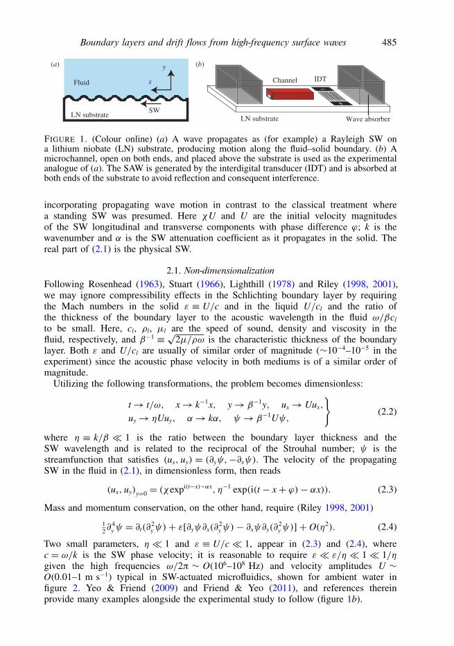
Consider the half space of a fluid above a solid substrate illustrated in figure 1(a);the coordinates x and y are measured along and transverse to the fluid–solid boundaryy = 0. A harmonic SW propagating on the boundary y = 0 with increasing x iscomposed of longitudinal and transverse displacements of similar amplitude, thevelocities of which are given by the form

(ux, uy)y=0 = (χU exp(i(ωt − kx)− αx),U exp(i(ωt − kx+ ϕ)− αx)), (2.1)

Boundary layers and drift flows from high-frequency surface waves 485

Wave absorber

IDTChannel

LN substrate

x

y

Fluid

LN substrateSW

(a) (b)

FIGURE 1. (Colour online) (a) A wave propagates as (for example) a Rayleigh SW ona lithium niobate (LN) substrate, producing motion along the fluid–solid boundary. (b) Amicrochannel, open on both ends, and placed above the substrate is used as the experimentalanalogue of (a). The SAW is generated by the interdigital transducer (IDT) and is absorbed atboth ends of the substrate to avoid reflection and consequent interference.

incorporating propagating wave motion in contrast to the classical treatment wherea standing SW was presumed. Here χU and U are the initial velocity magnitudesof the SW longitudinal and transverse components with phase difference ϕ; k is thewavenumber and α is the SW attenuation coefficient as it propagates in the solid. Thereal part of (2.1) is the physical SW.

2.1. Non-dimensionalizationFollowing Rosenhead (1963), Stuart (1966), Lighthill (1978) and Riley (1998, 2001),we may ignore compressibility effects in the Schlichting boundary layer by requiringthe Mach numbers in the solid ε ≡ U/c and in the liquid U/cl and the ratio ofthe thickness of the boundary layer to the acoustic wavelength in the fluid ω/βcl

to be small. Here, cl, ρl, µl are the speed of sound, density and viscosity in thefluid, respectively, and β−1 ≡√2µ/ρω is the characteristic thickness of the boundarylayer. Both ε and U/cl are usually of similar order of magnitude (∼10−4–10−5 in theexperiment) since the acoustic phase velocity in both mediums is of a similar order ofmagnitude.

Utilizing the following transformations, the problem becomes dimensionless:

t→ t/ω, x→ k−1x, y→ β−1y, ux→ Uux,

uy→ ηUuy, α→ kα, ψ→ β−1Uψ,

}(2.2)

where η ≡ k/β � 1 is the ratio between the boundary layer thickness and theSW wavelength and is related to the reciprocal of the Strouhal number; ψ is thestreamfunction that satisfies (ux, uy) = (∂yψ,−∂xψ). The velocity of the propagatingSW in the fluid in (2.1), in dimensionless form, then reads

(ux, uy)y=0 = (χexpi(t−x)−αx, η−1 exp(i(t − x+ ϕ)− αx)). (2.3)

Mass and momentum conservation, on the other hand, require (Riley 1998, 2001)

12∂

4yψ = ∂t(∂

2yψ)+ ε[∂yψ∂x(∂

2yψ)− ∂xψ∂y(∂

2yψ)] + O(η2). (2.4)

Two small parameters, η � 1 and ε ≡ U/c� 1, appear in (2.3) and (2.4), wherec = ω/k is the SW phase velocity; it is reasonable to require ε � ε/η � 1� 1/ηgiven the high frequencies ω/2π ∼ O(106–108 Hz) and velocity amplitudes U ∼O(0.01–1 m s−1) typical in SW-actuated microfluidics, shown for ambient water infigure 2. Yeo & Friend (2009) and Friend & Yeo (2011), and references thereinprovide many examples alongside the experimental study to follow (figure 1b).

486 O. Manor, L. Y. Yeo and J. R. Friend

2 5 10 20 50 100

10–4

SW frequency (MHz)

10–2

200

100

1

FIGURE 2. (Colour online) Variations in the non-dimensional parameters ε and ε/η overa range of frequencies (1–300 MHz) relevant to microfluidics for water atop 127.68◦ y-axisrotated, x-axis propagating LN (c∼ 4000 m s−1), a typical cut for microfluidics, subject to theRayleigh SW velocity amplitudes U = 0.01, 0.1 and 1 m s−1.

2.2. Asymptotic expansionSince (2.4) represents a boundary layer, an asymptotic flow field, it cannotsimultaneously satisfy both the conditions at the solid boundary (2.3) and the decay ofthe velocity field far from the solid. We then define the velocity at the solid boundaryby (2.3) and require ux to be bounded far from the solid boundary (Stuart 1966). Tosimplify the mathematical problem (2.3) and (2.4) are expanded in the asymptoticseries

ux =∞∑

n=−1

fnux,n, uy =∞∑

n=−1

fnuy,n, ψ =∞∑

n=−1

fnψn, (2.5)

where fn+1 � fn, and ux,n, uy,n and ψn are O(1). The transverse and longitudinalcomponents of the SW in (2.3) determine the leading magnitudes f−1 = 1/η and f0 = 1in the expansion of the velocity field.

2.3. Examination of O(1/η) and O(1) termsEquating the O(1/η) and O(1) terms, we find the corresponding components of thestreamfunction equation and the velocity at the solid boundary are

12∂

4yψ−1 = ∂t(∂

2yψ−1), (ux,−1, uy,−1)y=0 = (0, exp(i(t − x+ ϕ)− αx)), (2.6)

12∂

4yψ0 = ∂t(∂

2yψ0), (ux,0, uy,0)y=0 = (χei(t−x)−αx, 0). (2.7)

The requirements that ux is bounded far from the solid boundary and that the flow fieldmust satisfy (2.6) and (2.7), and the resultant distribution of the flow field along thesolid are all then represented to O(1/η) and O(1), respectively, by the equations

ψ−1|y=0 =−exp(i(t − x+ ϕ)− αx)

i+ α , ∂yψ−1|y=0 = 0,

−∂xψ−1|y=0 = exp(i(t − x+ ϕ)− αx),

(2.8)

ψ0|y=0 = 0, ∂yψ0|y=0 = χei(t−x)−αx, ∂xψ0|y=0 = 0, (2.9)

Boundary layers and drift flows from high-frequency surface waves 487

and by the condition that as y→∞, ψ−1 and ψ0 are not more singular than y. Theleading-order transverse unidirectional flow field is then

ψ−1 =− 1i+ α exp(i(t − x+ ϕ)− αx). (2.10)

Its sole component uy,−1 simply imitates the transverse component of the solidboundary velocity in (2.8) in order to conserve mass. Equations (2.7) and (2.9) aresatisfied by the leading-order Schlichting boundary layer flow field due to a travellingSW

ψ0 = χ(

12− i

2

)(1− e−(1+i)y) exp(i(t − x)− αx). (2.11)

Both flow fields in (2.10) and (2.11) are finite far from the solid boundary. It isinteresting to note that (2.11) satisfies only the O(1) longitudinal velocity of thesolid surface and remains independent of the O(1/η) transverse motion. The leadingperiodic flow field may thus be represented as a superposition of the unidirectionaltransverse flow in (2.10) and a solution similar to the classical leading-orderSchlichting boundary layer flow in (2.11) but incorporating the behaviour of the fluidas a consequence of travelling waves in addition to the classical treatment of standingwaves alone; this result is true regardless of the magnitudes of both flow fields.

We utilize this unusual scaling method in (2.2), where the leading-order term in theasymptotic analysis in (2.5) is large (i.e. O(1/η)� 1), in order to facilitate a directcomparison between magnitudes of the asymptotic flow components in this and earlierstudies: (2.11), consistently O(1), represents the leading-order flow both in earlierstudies and the second-order flow in the present study.

2.4. Examination of the O(ε/η) termThe next correction to the flow satisfies f1 = ε/η and the streamfunction equation andboundary conditions

12∂

4yψ1 = ∂t(∂

2yψ1)− ∂xψ−1∂

3yψ0, (ux,1, uy,1)y=0 = (0, 0). (2.12)

The requirement that ux is bounded far from the solid and the other constraints in(2.12) may then be represented to O(ε/η) by

ψ1|y=0 = ∂yψ1|y=0 = ∂xψ1|y=0 = 0 (2.13)

and by the condition that, as y→∞, ψ1 is not more singular than y. Since we areonly interested in the steady drift velocity ud, we follow Schlichting (1932), Stuart(1966) and Riley (1998, 2001), and decouple the velocity field into its transient andsteady components. The steady components of (2.12) and (2.13),

12∂

4y 〈ψ1〉 = −〈∂xψ−1∂

3yψ0〉, 〈ψ1〉|y=0 = ∂y〈ψ1〉|y=0 = ∂x〈ψ1〉|y=0 = 0, (2.14)

are satisfied by

〈ψ1〉 = χ2 e−2αx[−e−y sin(y+ ϕ)+ y cosϕ + (1− y) sinϕ]. (2.15)

Note ζ and 〈ζ 〉 above refer to the real component of the arbitrary function ζ and itstime average, such that 〈ζ 〉 ≡ (1/2π) ∫ 2π

0 ζ dt.Inertial interaction between the two leading-order periodic flow fields results in an

O(ε/η) correction to the flow that has a measurable non-vanishing steady component.

488 O. Manor, L. Y. Yeo and J. R. Friend

In earlier studies, where the flow field is derived for the excitation of one-dimensionalacoustic wave, the steady flow component (1.1) is O(U/cl).

From the ansatz in (2.5), the streamfunction then reads

ψ =− 1η(i+ α) exp(i(t − x+ ϕ)− αx)

+χ(

12− i

2

)[1− e−(1+i)y]e−αxei(t−x) + · · · ; (2.16)

and its steady component is

〈ψ〉 = εη

χ

2e−2αx[−e−y sin(y+ ϕ)+ y cosϕ + (1− y) sinϕ] + · · · . (2.17)

In the asymptotic limit y→∞, the dimensional longitudinal and transverse driftvelocities found from (2.17) at the outer edge of the boundary layer are then

udx ∼ εη

χU

2e−2αx(cosϕ − sinϕ),

ε

η

χU

2≡ χU2

2

√ρ

2µω, (2.18)

udy ∼ εχUβyαxe−2αx(cosϕ − sinϕ). (2.19)

The direction and magnitude of the drift velocity (2.18) depend on the phasedifference between the longitudinal and transverse components of the SW; itsmagnitude monotonically decreases as the SW attenuates and does not vanish whenthe amplitude of the SW excitation is independent of the spatial coordinate, unlikein (1.1). Under pure retrograde motion (e.g. for Rayleigh SAWs, ϕ = 3π/2), the driftvelocity is in the direction of SW propagation whereas under pure prograde motion(e.g. for Sezawa SAWs, ϕ = π/2), the drift velocity opposes the direction of SWpropagation. A similar relation between the drift velocity and phase was obtained byRamos, Cuevas & Huelsz (2001) under the excitation of a longitudinal oscillating platethat is being impinged by transverse bulk waves; both oscillate at the same frequency.

2.5. Analysis of closed-channel flow must include bulk acoustic waves in the fluidFurther analysis is, however, required for microfluidic flows where fluids tend tobe in closed structures, such as channels, rather than a half-space as treated before,due to the presence of acoustic waves in both the fluid bulk and the boundarylayer. While structural dimensions large compared with the characteristic length ofthe boundary layer β−1 will satisfy the half-space geometry of the theory presentedherein to a good approximation, closed geometries under the excitation of SWs havebeen experimentally and analytically found to support acoustic wave propagation andinteraction in the bulk of the fluid, forming standing bulk acoustic waves over longdistances (Craster 1996; Hamilton 2003; Tan et al. 2009). Bulk acoustic waves aregenerated from attenuating boundary SWs at the Rayleigh angle and their reflectionoccurs due to a change in acoustic impedance at the boundary. The amplitude of thereflected wave depends upon the material and configuration details but is very oftensignificant and difficult to suppress in microfluidic platforms. Boundary conditionspermitting both a propagating boundary SW and a standing bulk wave tangent to thatboundary may be written in generalized dimensional form as (2.1) and

(ux, uy)βy→∞ = (2χUeiωt cos(δkx), 0), (2.20)

Boundary layers and drift flows from high-frequency surface waves 489

where δ ≡ c/cl. The bulk wave is constructed from identical advancing and recedinglongitudinal waves, emerging from SW-induced vibrations of the channel along thesolid boundary (2.20) and describing a bulk wave possessing the frequency, phase andvelocity amplitude of the longitudinal component of the SW.

Following a similar procedure, (2.2), (2.3), (2.4) and (2.5) suggest that the O(1/η)leading-order component of the streamfunction equation and boundary conditions aregiven by (2.6), (2.8), and the condition that the streamfunction is not more singularthan y as y→∞; these are satisfied by (2.10). Furthermore, the O(1) component ofthe streamfunction equation and boundary conditions are given now by (2.7), (2.9),and (2.20). We then decompose the linear O(1) problem to two simplified problems:the flow under the influence of the bulk wave (2.20) and the flow under the influenceof the SW in (2.9). The former is described by (2.7), (2.20), and (ux, uy)|y=0 = (0, 0); asolution is provided by Stuart (1966) and Riley (1998, 2001). The latter, on the otherhand, is described by (2.7), (2.9) and a stream function that is no more singular thany as y→∞, with a solution given by (2.11). The O(1) flow field in the presence ofboth the SW and the bulk wave is then the superposition of both solutions, given in adimensionless form as

ψ0 = 2χ cos(δx){

y− 12(1− i)[1− e−(1+i)y]eit

+χ(

12− i

2

)[1− e−(1+i)y]e−αxei(t−x)

}. (2.21)

The O(ε/η) steady components of the streamfunction equation and boundaryconditions (2.14) together with the requirement that ux is bounded far from the solidare then satisfied by

〈ψ1〉 = χ [e−(y+2αx)]

2{ey[y cosϕ + (1− y) sinϕ] − sin(y+ ϕ)

− 2eαx cos(δx){ey[y cos(x− ϕ)+ (y− 1) sin(x− ϕ)] + sin(x− y− ϕ)}}. (2.22)

In the asymptotic limit y→∞, the dimensional drift velocities along and transverse tothe solid boundary,

udx∼ εη

χU

2e−2αkx{{cosϕ − sinϕ − 2eαkx cos(δkx)

×[cos(kx− ϕ)+ sin(kx− ϕ)]}},ε

η

χU

2≡ χU2

2

√ρ

2µω,

(2.23)

and

udy ∼ εχβUye−2αkx{−eαkx{cos(kx− ϕ)[(−1+ α) cos(δkx)+ δ sin(δkx)]+ sin(kx− ϕ)[(1+ α) cos(δkx)+ δ sin(δkx)]} + α(cosϕ − sinϕ)}, (2.24)

conserve both the SW and bulk wavelength scales λ = 2π/k and λl = 2π/δk,respectively; this is apparent as we graphically present (2.23) in the next section.

Following Stuart (1966) we may treat the longitudinal drift velocity udx as theleading-order outer expansion of the inner boundary layer. Ignoring smaller ordercorrections, matching udx to the inner expansion of the outer flow field (i.e. the flowoutside the boundary layer) is equivalent to using udx as a slip velocity boundarycondition for the outer velocity field: Rayleigh’s law of streaming. The longitudinal

490 O. Manor, L. Y. Yeo and J. R. Friend

drift velocity udx in (2.18) or (2.23) is then the appropriate asymptotic boundarycondition for bulk flow under the influence of a propagating SWs. The O(ε) transversedrift velocity udy in (2.19) or (2.24), on the other hand, can usually be ignored. Wenow seek to validate this theory with a simple experiment.

3. ExperimentA Rayleigh SW is made to propagate along a piezoelectric substrate, inducing

boundary layer flow within a microchannel placed atop the substrate as depicted infigure 1(b). The Schlichting boundary layer cannot be directly observed since itsthickness is generally less than 1 µm under high-frequency excitation, and so weseek to observe the influence of the steady drift velocity on the outer flow field inthe vicinity of the solid boundary. The outer flow field is also influenced by Eckartstreaming, generated in the bulk of the channel due to the attenuation of acousticwaves emitted, in this case, by the Rayleigh SW (Lighthill 1978). We identify theexistence of this particular flow by the steady vortices it generates in the bulk of thechannel. This vortical flow has a dispersive influence on the drift velocity developed atthe outer edge of the boundary layer. Choosing slender channels (i.e. microchannels)made from material that absorbs and damps the acoustic wave, the Eckart streamingis retarded by viscous effects and reduced in amplitude in its interactions with thechannel wall, and in this way we enhance the relative influence of the drift velocity.Nevertheless, weak Eckart streaming was still observed to partially disperse the flowfield in the vicinity of the solid substrate over a substantial portion of the channel.

3.1. Experimental setup

We employ a 3.2 × 107 Hz Rayleigh SW device comprising a 10 nm chrome/250 nmaluminum interdigital transducer (IDT) electrode patterned using standard UVphotolithography on a 0.5 mm thick 128◦ Y-cut, X-propagating single-crystal lithiumniobate (LN) piezoelectric substrate (Tan, Friend & Yeo 2007b; Qi et al. 2008).Absorbent material (α-gel, Geltec Ltd, Yokohama, Japan), placed at the ends ofthe substrate, eliminates wave reflections as depicted in figure 1(b). The SW isgenerated by applying a sinusoidal electric voltage to the IDT using a signalgenerator (SML01; Rhode and Schwarz, North Ryde, NSW, Australia) and amplifier(10W1000C; Amplifier Research, Souderton, PA); an oscilloscope (Wavejet 332/334;LeCroy, Chestnut Ridge, NY) was used to measure the actual voltage across thedevice. Spatial variations of the velocity amplitude U of the transverse SW along thesolid boundary was measured using a laser Doppler vibrometer (LDV; UHF–120,Polytec GmBH, Waldbronn, Germany); the measurements verified that the SWgenerated here is indeed a propagating Rayleigh SW.

Microchannels, 80 µm thick and 1 mm wide, were prepared by mold-curing 3 mmthick polydimethylsiloxane (PDMS) (Sylgard 184; Dow Corning, Midland, MI) in astandard process (Friend & Yeo 2009) and then filled with a highly dilute suspension(0.003 vol %) of 1 and 5 µm fluorescent polystyrene spheres (Duke Scientific Corp.,Fremont, CA) in deionized water (Millipore, Billerica, MA) and attached to the LNsubstrate following the procedure in Girardo et al. (2008). The size of the polystyrenespheres was chosen to ensure the hydrodynamic drag exerted by the fluid dominatedthe direct acoustic radiation force from the bulk wave in the fluid (Rogers, Friend &Yeo 2010). The flow field in the vicinity of the substrate was acquired using an uprightfluorescence microscope coupled to a high-speed camera (BX–FM stereomicroscopeand iSpeed camera, Olympus, Yokohama, Japan) and measured both before and after

Boundary layers and drift flows from high-frequency surface waves 491

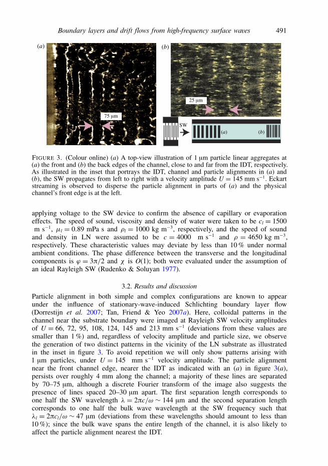
(a) (b)

SW(a) (b)

FIGURE 3. (Colour online) (a) A top-view illustration of 1 µm particle linear aggregates at(a) the front and (b) the back edges of the channel, close to and far from the IDT, respectively.As illustrated in the inset that portrays the IDT, channel and particle alignments in (a) and(b), the SW propagates from left to right with a velocity amplitude U = 145 mm s−1. Eckartstreaming is observed to disperse the particle alignment in parts of (a) and the physicalchannel’s front edge is at the left.

applying voltage to the SW device to confirm the absence of capillary or evaporationeffects. The speed of sound, viscosity and density of water were taken to be cl = 1500m s−1, µl = 0.89 mPa s and ρl = 1000 kg m−3, respectively, and the speed of sound

and density in LN were assumed to be c = 4000 m s−1 and ρ = 4650 kg m−3,respectively. These characteristic values may deviate by less than 10 % under normalambient conditions. The phase difference between the transverse and the longitudinalcomponents is ϕ = 3π/2 and χ is O(1); both were evaluated under the assumption ofan ideal Rayleigh SW (Rudenko & Soluyan 1977).

3.2. Results and discussionParticle alignment in both simple and complex configurations are known to appearunder the influence of stationary-wave-induced Schlichting boundary layer flow(Dorrestijn et al. 2007; Tan, Friend & Yeo 2007a). Here, colloidal patterns in thechannel near the substrate boundary were imaged at Rayleigh SW velocity amplitudesof U = 66, 72, 95, 108, 124, 145 and 213 mm s−1 (deviations from these values aresmaller than 1 %) and, regardless of velocity amplitude and particle size, we observethe generation of two distinct patterns in the vicinity of the LN substrate as illustratedin the inset in figure 3. To avoid repetition we will only show patterns arising with1 µm particles, under U = 145 mm s−1 velocity amplitude. The particle alignmentnear the front channel edge, nearer the IDT as indicated with an (a) in figure 3(a),persists over roughly 4 mm along the channel; a majority of these lines are separatedby 70–75 µm, although a discrete Fourier transform of the image also suggests thepresence of lines spaced 20–30 µm apart. The first separation length corresponds toone half the SW wavelength λ = 2πc/ω ∼ 144 µm and the second separation lengthcorresponds to one half the bulk wave wavelength at the SW frequency such thatλl = 2πcl/ω ∼ 47 µm (deviations from these wavelengths should amount to less than10 %); since the bulk wave spans the entire length of the channel, it is also likely toaffect the particle alignment nearest the IDT.

492 O. Manor, L. Y. Yeo and J. R. Friend

Further along the channel, beyond 4 mm, the patterns disappear leaving apparentlyrandomly dispersed particles, likely due to both the dispersive influence of Eckartstreaming that is most significant in the middle of the channel and the rapidexponential attenuation of the SW in the substrate. The SW attenuation lengthα−1 ∼ Fρcλ/(ρlcl) ∼ 1 mm renders the SW amplitude small beyond 3α−1–4α−1 mm;F−1 ≈ 1.4 is a correction for the anisotropy of the LN substrate (Arzt, Salzmann &Dransfeld 1967; Cheeke & Morisseau 1982).

Roughly 1 mm from the back channel edge, opposite the IDT, the particles onceagain align in the vicinity of the LN substrate into fine lines with a separation lengthof approximately 25 µm (figure 3b), corresponding to the bulk wave wavelength at theSW frequency λl. Since the SW attenuates before reaching the far end of the channel,we may suppose the excitation there is a SW-induced bulk wave in the fluid domain.The bulk wave is a standing acoustic wave bounded by the fully reflecting air/waterinterfaces at both channel ends. This hypothesis was assessed by adding water tothe channel back end, opposite the IDT, to fill the gap between the channel and thewave absorber, essentially replacing the fully reflecting air/water interface at that endwith a poorly reflecting water/wave absorber interface. This was found to suppressthe particle alignment in the channel, indicating the bulk wave was likewise absentsince pure propagating SW alone generates the drift velocity in (2.18) that does notsustain stagnant areas where particles may aggregate into patterns. We further examinethe formation of these aggregation lines by substituting the boundary condition forthe SW-induced bulk wave (2.20) into (1.1). This procedure is similar to the classicalsolution by Stuart (1966) for the drift velocity in a boundary layer excited by a bulkwave. The boundary condition on the substrate in the absence of the Rayleigh SW(ux, uy) = (0, 0) at y = 0 is then satisfied. The dimensional drift velocity in terms ofthe bulk wave wavelength λl = 2π/δk,

udx/U ∼ U

clχ 2 cos(2πx/λl) sin(2πx/λl), (3.1)

is shown in figure 4(b). Each wavelength λl contains two stable stagnation pointswhere ud = 0, dud/dx < 0 are satisfied, and where particles align. Two unstablestagnant points, satisfying ud = 0, dud/dx > 0, are also present but represent locationsthat particles avoid; this is in good agreement with observations.

The difference in particle aggregate patterns near and far away from the IDT, andthe different spacing of lines associated with the wavelengths of the bulk wave andSW, respectively, altogether imply a mutual contribution by both the bulk wave andthe SW to forming patterns of particles in the channel. We quantify this assertion bysubstituting the properties of a Rayleigh SW (ϕ = 3π/2) and a corresponding bulkwave in (2.23) and comparing the expression for the drift velocity

udx/U ∼ εη

χ

2{e−2αkx − 2e−αkx cos(2πx/λl)[cos(2πx/λ)− sin(2πx/λ)]}, (3.2)

to the patterns in figure 4(a). The good agreement between the stable stagnationregions (ud = 0, dud/dx < 0) generated by the drift velocity (3.2) and the aggregationline patterns in the experiment infers the complicated interaction between SWs andbulk waves within the flow field. The minor difference in the theoretical predictionand experimental result can be attributed to the possible deviations in the characteristicvalues of the material properties used. Note the denser patterns of particles underO(ε/η) drift flow near the IDT compared with the patterns under O(ε) drift flow farfrom the IDT; the density of the patterns is determined in part by a balance between

Boundary layers and drift flows from high-frequency surface waves 493

(a) (b)

0.5

1 2 3

1 2

–0.5

0.5

1.5

–0.5

FIGURE 4. (Colour online) Spatial comparison between the theoretical variation of the driftvelocity along the solid boundary (positive values refer to flow in the direction of thepropagating SW, left to right in the images) and the particle alignments in figure 3 due tothe presence of a bulk wave for (a) 1 µm polystyrene particles with SW, depicted in (3.2),and (b) without SW, depicted in (3.1). Dashed lines connect stable stagnant flow points whereparticles are predicted to accumulate (driven by the drift flow from both sides) with theparticle alignments observed in the experiment: (a) udx/[(ε/η)χ U]; (b) udx/[(U/cl)χ2 U].

the ordered drift flow and the dispersive effects of particle diffusion and Eckart flow,suggesting that the drift flow is dominant where the particle patterns are most denseand physically illustrating the utility of the scaling used in this study.

4. ConclusionsThe classical Schlichting boundary layer theory was extended to include two-

dimensional, potentially propagating SW at frequencies and substrate velocitiestypically employed in microfluidic platforms. The steady drift velocity due to apropagating SW was asymptotically derived, indicating it is O(ε/η) under theexcitation of a two-dimensional SW that possesses comparable longitudinal andtransverse amplitude components. This result generally dominates the classicalO(U/cl) result that is valid only under the excitation of a simpler one-dimensionalacoustic wave.

An additional result was derived for the steady drift velocity in a boundary layerarising from the excitation of both a two-dimensional SW at the solid boundary andan additional standing acoustic wave present throughout the fluid and that possessessimilar frequency, phase and velocity characteristics to the SW. This configuration isoften present in microfluidic platforms where microflows are enclosed within acousticwave reflecting structures, such as channels, where SWs give rise to such secondarybulk waves. Weak inertial interaction between the leading superimposed flow fields

494 O. Manor, L. Y. Yeo and J. R. Friend

resulting from both wave excitations gives rise to a complex, steady and non-vanishingdrift velocity that preserves properties from both wave forms.

Good agreement between theory and experiment was found for flow in amicrochannel atop a piezoelectric substrate, where high-frequency Rayleigh SWexcites a secondary stationary bulk wave in the channel and subsequent Schlichtingboundary layer flow; the resultant steady drift velocity observed exhibits characteristicsof both wave types in colloidal particle alignments. Finally, the analytical expressionderived for the drift velocity may be employed as an effective slip velocity boundarycondition for the bulk flow. Further, in the presence of O(U/cl) slow Eckart streaming,the O(ε/η) drift velocity should dominate the bulk flow. In the presence of O(1)fast Eckart streaming, however, drift velocity effects are likely to be dispersed;nevertheless, the drift velocity exists in the vicinity of the solid substrate and becomesapparent where the bulk flow is stagnant.

R E F E R E N C E S

ALVAREZ, M., FRIEND, J. R. & YEO, L. Y. 2008 Surface vibration induced spatial ordering ofperiodic polymer patterns on a substrate. Langmuir 24, 10629–10632.

ARZT, R. M., SALZMANN, E. & DRANSFELD, K. 1967 Elastic surface waves in quartz at 316 MHz.Appl. Phys. Lett. 10, 165–167.

BRUNET, P., BAUDOIN, M., MATAR, O. & ZOUESHTIAGH, F. 2010 Droplet displacements andoscillations induced by ultrasonic surface acoustic waves: a quantitative study. Phys. Rev. E81, 036315.

CHEEKE, J. D. N. & MORISSEAU, P. 1982 Attenuation of Rayleigh waves on a LiNbO3 crystal incontact with a liquid He bath. J. Low Temp. Phys. 46, 319–330.

CHLADNI, E. 1787 Entdeckungen uber die Theorie des Klanges. Weidmanns, Erben und Reich.CRASTER, R. V. 1996 A canonical problem for fluid–solid interfacial wave coupling. Proc. R. Soc.

Lond. A 452, 1695–1711.DORRESTIJN, M., BIETSCH, A., ACKALN, T., RAMAN, A., HEGNER, M., MEYER, E. & GERBER,

C. H. 2007 Chladni figures revisited based on nanomechanics. Phys. Rev. Lett. 98, 026102.ECKART, C. 1948 Vortices and streams caused by sound waves. Phys. Rev. 73, 68–76.FARADAY, M. 1831 On a peculiar class of acoustical figures; and on certain forms assumed by

groups of particles upon vibrating elastic surfaces. Phil. Trans. R. Soc. Lond. 121, 299–340.FRIEND, J. R. & YEO, L. Y. 2009 Fabrication of microfluidics devices using polydimethylsiloxane

(PDMS). Biomicrofluidics 4, 026502.FRIEND, J. R. & YEO, L. Y. 2011 Microscale acoustofluidics: microfluidics driven via acoustics and

ultrasonics. Rev. Mod. Phys. 83, 647–704.GIRARDO, S., CECCHINI, M., BELTRAM, F., CINGOLANI, R. & PISIGNANO, D. 2008

Polydimethylsiloxane–LiNbO3 surface acoustic wave micropump devices for fluid control inmicrochannels. Lab on a Chip 8, 1557–1563.

HAMILTON, M. 2003 Acoustic streaming generated by standing waves in two-dimensional channelsof arbitrary width. J. Acoust. Soc. Am. 113, 153–160.

HODGSON, R. P., TAN, M., YEO, L. Y. & FRIEND, J. R. 2009 Transmitting high power rf acousticradiation via fluid couplants into superstrates for microfluidics. Appl. Phys. Lett. 94, 024102.

HOLTSMARK, J., JOHNSEN, I., SIKKELAND, T. & SKAVL, S. 1954 Boundary layer flow near acylindrical obstacle in an oscillating, incompressible fluid. J. Acoust. Soc. Am. 26, 26–39.

HUTCHISSON, E. & MORGAN, F. B. 1931 An experimental study of Kundt’s tube dust figures. Phys.Rev. 37, 1155–1163.

LI, H., FRIEND, J. R. & YEO, L. Y. 2008 Microfluidic colloidal island formation and erasureinduced by surface acoustic wave radiation. Phys. Rev. Lett. 101, 084502.

LIGHTHILL, J. 1978 Acoustic streaming. J. Sound Vib. 61, 391–418.LONGUET-HIGGINS, M. S. 1953 Mass transport in water waves. Phil. Trans. R. Soc. Lond. 245,

535–581.

Boundary layers and drift flows from high-frequency surface waves 495

LUONG, T.-D., PHAN, V.-N. & NGUYEN, N.-T. 2011 High-throughput micromixers based onacoustic streaming induced by surface acoustic wave. Microfluid Nanofluid 10, 619–625.

NAM, J., LIM, H., KIM, D. & SHIN, S. 2011 Separation of platelets from whole blood usingstanding surface acoustic waves in a microchannel. Lab on a Chip 11, 3361.

NYBORG, W. L. 1952 Acoustic streaming due to attenuated plane waves. J. Acoust. Soc. Am. 25,1–8.

QI, A., YEO, L. Y. & FRIEND, J. R. 2008 Interfacial destabilization and atomization driven bysurface acoustic waves. Phys. Fluids 20, 074103.

RAMOS, E., CUEVAS, S. & HUELSZ, G. 2001 Interaction of Stokes boundary layer flow with soundwave. Phys. Fluids 13, 3709–3713.

RAYLEIGH, LORD 1884 On the circulation of air observed in Kundt’s tubes and on some alliedacoustical problems. Phil. Trans. R. Soc. Lond. 175, 1–21.

RILEY, N. 1965 Oscillating viscous flows. Mathematika 12, 161–175.RILEY, N. 1986 Streaming from a cylinder due to an acoustic source. J. Fluid Mech. 180, 319–326.RILEY, N. 1998 Acoustic streaming. Theor. Comput. Fluid Dyn. 10, 349–356.RILEY, N. 2001 Steady streaming. Annu. Rev. Fluid Mech. 33, 43–65.ROGERS, P. P., FRIEND, J. R. & YEO, L. Y. 2010 Exploitation of surface acoustic waves to drive

size-dependent microparticle concentration within a droplet. Lab on a Chip 10, 2979–2985.ROSENHEAD, L. (Ed.) 1963 Laminar Boundary Layers. Oxford Engineering: Clarendon.RUDENKO, O. V. & SOLUYAN, S. I. 1977 Theoretical Foundations of Nonlinear Acoustics.

Plenum.SCHLICHTING, H. 1932 Calculation of even periodic barrier currents. Physik. Z. 33, 327–335.SECOMB, T. W. 1978 Flow in a channel with pulsating walls. J. Fluid Mech. 88, 273–288.SHI, J., HUANG, H., STRATTON, Z., HUANG, Y. & HUANG, T. J. 2009 Continuous particle

separation in a microfluidic channel via standing surface acoustic waves (SSAW). Lab on aChip 9, 3354–3359.

STUART, J. T. 1966 Double boundary layers in oscillatory viscous flow. J. Fluid Mech. 24,673–687.

TAN, M. K., FRIEND, J. R. & YEO, L. Y. 2007a Direct visualization of surface acoustic wavesalong substrates using smoke particles. Appl. Phys. Lett. 91, 224101.

TAN, M. K., FRIEND, J. R. & YEO, L. Y. 2007b Microparticle collection and concentration via aminiature surface acoustic wave device. Lab on a Chip 7, 618–625.

TAN, M. K., YEO, L. Y. & FRIEND, J. R. 2009 Rapid fluid flow and mixing induced inmicrochannels using surface acoustic waves. Eur. Phys. Lett. 87, 1–6.

WANG, C. Y. 2005 On high-frequency oscillatory viscous flows. J. Fluid Mech. 32, 55–68.WESTERVELT, P. J. 2004 The theory of steady rotational flow generated by a sound field. J. Acoust.

Soc. Am. 25, 60–67.WIXFORTH, A., STROBL, C., GAUER, C., TOEGL, A., SCRIBA, J. & VON GUTTENBERG, Z. 2004

Acoustic manipulation of small droplets. Anal. Bioanal. Chem. 379, 982–991.YEO, L. Y. & FRIEND, J. R. 2009 Ultrafast microfluidics using surface acoustic waves.

Biomicrofluidics 3, 012002.ZENG, Q., CHAN, H. W. L., ZHAO, X. Z. & CHEN, Y. 2010 Enhanced particle focusing

in microfluidic channels with standing surface acoustic waves. Microelectron. Engng 87,1204–1206.