Author's personal copy

A model of dynamic compensation and capital structure$

Zhiguo He

University of Chicago, Booth School of Business, United States

a r t i c l e i n f o

Article history:

Received 16 June 2009

Received in revised form

19 April 2010

Accepted 22 May 2010Available online 2 February 2011

JEL classification:

G32

D86

J33

Keywords:

Continuous-time contracting

Capital structure

CARA (exponential) preference

Firm growth

Size-heterogeneity

Pay-performance sensitivity

a b s t r a c t

This paper studies the optimal compensation problem between shareholders and the

agent in the Leland (1994) capital structure model, and finds that the debt-overhang

effect on the endogenous managerial incentives lowers the optimal leverage. Consistent

with data, our model delivers a negative relation between pay-performance sensitivity

and firm size, and the interaction between debt-overhang and agency issue leads

smaller firms to take less leverage relative to their larger peers. During financial

distress, a firm’s cash flow becomes more sensitive to underlying performance shocks

due to debt-overhang. The implications on credit spreads and debt covenants are also

considered.

Published by Elsevier B.V.

1. Introduction

This paper embeds optimal contracting between theagent (manager) and shareholders into the cash flowframework commonly used in the literature of structuralmodels of capital structure (Leland, 1994). By connectingthese two literatures, I provide a general framework tostudy the impact of agency characteristics on firm valua-tion and capital structure. Moreover, the dynamic natureof this framework allows me to calibrate my model and,in turn, quantitatively assess the agency impact on thefirm’s leverage decision.

I characterize the optimal contract between share-holders and the agent explicitly. In determining theleverage level, debt bears an additional ‘‘debt-overhang’’cost relative to the bankruptcy cost in standard models(a la Leland, 1994): By interpreting the agent’s effort as aform of investment, shareholders implement diminishingeffort (as cut back investment) during financial distress.As a result, the agency problem reduces the optimalleverage from 63.2% based on Leland (1994, with mycalibration) to as low as 39.5%. Consistent with the data,my model predicts that small firms take less leveragerelative to their large peers. The debt-overhang problemalso implies that the firm’s cash flow is more sensitiveto underlying shocks, reinforcing the standard leverageeffect.

Section 2 starts by offering a general analysis in solvingthe optimal contracting problem. The analysis hinges onthe agent’s constant absolute risk aversion (CARA, orexponential) preference. In contrast to Holmstrom andMilgrom (1987), in which the lump-sum compensation is

Contents lists available at ScienceDirect

journal homepage: www.elsevier.com/locate/jfec

Journal of Financial Economics

0304-405X/$ - see front matter Published by Elsevier B.V.

doi:10.1016/j.jfineco.2011.01.005

$ An earlier version of this paper was circulated under the title

‘‘Agency Problems, Firm Valuation, and Capital Structure.’’ I thank the

referee Hayne Leland. Mike Fishman, Arvind Krishnamurthy, Patrick

Bolton, Chris Hennessy, Debbie Lucas, Ilya Strabeleuv, and Yuri Tserlu-

kevich (AFA 2009 discussant) for valuable suggestions. All errors are

mine.

E-mail address: Zhiguo.he@chicagobooth.edu

Journal of Financial Economics 100 (2011) 351–366

Author's personal copy

considered, the agent in my model has intermediateconsumption flows and can privately save. To solve forthe optimal contract, I employ the approach in Sannikov(2008) and take the agent’s continuation value (continua-tion payoff or promised utility) as one state variable. Theabsence of wealth effect under CARA preference allowsme to characterize the optimal contract by an ordinarydifferential equation (ODE) in Section 2.3. I derive the(second-best) firm value and the agent’s pay-performancesensitivity (PPS, the dollar-to-dollar measure as in Jensenand Murphy, 1990) based on the optimal contracting. Ialso characterize the condition that ensures the empiricalregularity of an inverse relation between the agent’s pay-performance sensitivity and firm size.

Section 3 applies the optimal contracting result to theframework in Leland (1994). There, the firm growth isendogenously affected by the agent’s effort, and in theoptimal contract both the pay-performance sensitivity andthe firm growth are decreasing in firm size. To investigatethe impact of agency issues on capital structure, Section3.3 introduces debt into the baseline model. For bettercomparison with Leland (1994) and other related work,I leave the debt contract to take the same form as in Leland(1994). Specifically, only consol bond is considered, andshareholders have the option to default when the firmprofitability deteriorates. On the contracting side, I bondthe agent and shareholders together through an optimalcontract solved in Section 2.1 Furthermore, shareholdersand the agent can revise the compensation contractdynamically, so that the compensation contract is a bestresponse to the capital structure.2 Essentially, these sim-plifying assumptions capture the key notion that, inUnited States corporations, managers are responsible onlyto shareholders (e.g., Brealey, Myers, and Allen, 2006).

I then solve for the optimal capital structure and theoptimal employment contract in Section 3.3. Comparedwith Leland (1994), my model features a debt-overhangproblem. Specifically, in my endogenous firm growthframework in which the firm growth is controlled bythe manager or shareholders or both, when close tobankruptcy shareholders assign diminishing incentivesto the agent. This result is due to debt-overhang, i.e.,reducing the positive net present value (NPV) effortinvestment in financially distressed firms. In other words,beyond the standard bankruptcy cost, debt bears anotherform of cost, as debt-overhang interferes with agencyissues. As a result, my model produces lower optimalleverage ratios relative to the Leland (1994) benchmark.

The debt-overhang generates a negative relationbetween leverage and agent’s working incentives, a predic-tion opposite to Cadenillas, Cvitanic, and Zapatero (2004),

in which the debt level and agent’s incentives are positivelyrelated. In that paper, they study a dynamic compensationand capital structure model in which the agent controlsboth the drift (effort) and the volatility (project selection) ofthe firm value. There, the agent’s compensation space isrestricted to equity shares, and shareholders commit to thisstatic compensation scheme. Setting a higher leveragedirectly reduces the value of the agent’s equity compensa-tion. Under their assumption of the agent having log utility,this induces a higher sensitivity of the agent’s value to hisperformance and, therefore, stronger working incentives. Incontrast, I show that in a dynamic model, if shareholdersand the agent can revise the compensation contract expost,3 then there is an opposite effect in addition to thesechannels, and it is an empirical question of which forceprevails under various economic circumstances.

Further, the interaction between agency issue and debt-overhang predicts that smaller firms take less leverage,which is consistent with empirical regularity. In my model,shareholders in small firms implement a higher effort (or,higher investment) without debt, which matches the empiri-cally observed negative relation between pay-performancesensitivities and firm sizes. Because the presence of debt cutsback effort investment, debt-overhang becomes more severein small firms. Taking this higher debt-overhang cost intoaccount, small firms choose a lower optimal leverage. In mycalibrations for small firms, the predicted optimal leverageratios, with or without the agency issue, can have a sizeabledifference (63.2% versus 39.5%).

In the literature, several attempts have been made toincorporate other important agency issues into the cor-porate security pricing setting. For instance, Leland (1998)studies the risk-shifting issue due to the endogenouschoice of firm’s volatility; there, the agent and share-holders are treated as one party. This paper focuses ondebt-overhang.4 Moreover, this paper distinguishes itselffrom the above mentioned literature in that I study theagency impact based on the optimal dynamic contractingapproach. Even though it seems appealing to restrict thecompensation contract space within commonly observedforms as in Cadenillas, Cvitanic, and Zapatero (2004), onemight wonder whether the derived impact of agencyproblems is sensitive to specific contract forms.5 Theoptimal contracting approach is free of this issue.

1 In my model, the agent, once bonded with shareholders by an

optimal contract, has perfectly aligned interest with shareholders when

dealing with debt holders. As a result, the default policy is independent

of whether shareholders or the agent control the bankruptcy decision.

This is different from Morellec (2004), in which the agent tends to keep

the firm alive longer for more private benefit.2 This assumption can be justified by the fact that, under this CARA

framework, the long-term contract is renegotiation-proof and can be

implemented by a sequence of short-term contracts (see Fudenberg,

Holmstrom, and Milgrom, 1990).

3 This assumption is consistent with both the practice of resetting

the strike price of stock options, and the empirical results in Bryan,

Hwang, and Lilien (2000) who investigate the stock-based compensa-

tions in a panel of firms (see footnote 29 for more details).4 Based on the free cash flow problem, Morellec (2004) introduces a

tension between the agent and shareholders, and the empire-building

agent tends to set a lower leverage ratio for rent-maximizing

purposes. Cadenillas, Cvitanic, and Zapatero (2004) study a different

version of agency problem, in which they restrict the compensation

contract space to be equity. Because the equity payoff ties to the debt

face value, in their model the capital structure becomes a direct

compensation scheme. In contrast, in my model the impact of leverage

decision on the compensation contract is indirect.5 Technically speaking, in the aforementioned papers, either the

volatility choice in Leland (1998) which is observable in Brownian setting,

or the over-investment (observable) decision in Morellec (2004), can be

easily resolved by optimal contracting. These extreme examples illustrate

the sensitivity of agency costs to the contracting space.

Z. He / Journal of Financial Economics 100 (2011) 351–366352

Author's personal copy

This paper is also related to the ongoing continuous-timecontracting literature. Sannikov (2008) studies a generaldynamic agency problem without private savings. Williams(2006) focuses on the general hidden-state problem andsolves an example with CARA preference. My paper, basedon the continuation value approach advocated in Sannikov(2008), analyzes the general cash flow setup and focuses onthe applications to corporate finance. DeMarzo and Fishman(2007), DeMarzo and Sannikov (2006), and Biais, Mariotti,Plantin, and Rochet (2007) solve a dynamic contractingproblem with a risk-neutral agent, in which the limitedliability restriction is imposed.6 In contrast, this paper takesthe Holmstrom and Milgrom (1987) framework, which notonly allows for a risk-averse agent, but also easily accom-modates a second state variable to capture the firm’s time-varying profitability.7 Compared with Holmstrom andMilgrom (1987), I allow for the agent’s intermediate con-sumption, and therefore their approach is no longerapplicable.

The rest of this paper is organized as follows. Section 2derives an ODE that characterizes the optimal contrac-ting, and Section 3 applies the contracting result toLeland (1994). Section 4 concludes. All proofs are in theAppendix.

2. General model and optimal contracting

In this section, I first study the optimal contractingproblem in a model with general cash flow process. Thenbased on the implementation of the optimal contract, Idiscuss its implications on pay-performance sensitivities(PPS) in executive compensation.

2.1. General model

I study an infinite-horizon, continuous-time agencyproblem. The firm (shareholders) hires an agent to oper-ate the business. The firm produces cash flows dt per unitof time, where dt follows the stochastic process

ddt ¼ mðdt ,atÞ dtþsðdtÞ dZt : ð1Þ

I also interpret dt as firm size in this paper. Throughunobservable effort at 2 ½0,a�, the agent controls the cashflow growth rate mðdt ,atÞ, where maðd,aÞ � @mðd,aÞ=@a40and maaðd,aÞ � @2mðd,aÞ=@a2r0. The performances fdtg arecontractible.

Shareholders (the principal) are risk-neutral, andthey discount future cash flows at the constant marketinterest rate r. To focus on the optimal contracting,

throughout Section 2 the firm is unlevered. I will intro-duce debt holders in Section 3.

The agent, with a CARA instantaneous utility and atime discounting factor r, maximizes his expected lifetime utility

E

Z 10�

1

g e�gðct�gðdt ,at ÞÞ�rt dt

� �,

where ct 2 R is the agent’s consumption rate and gðd,aÞ isthe agent’s monetary effort cost with gaðd,aÞ ¼ @gðd,aÞ=@a40 and gaaðd,aÞ ¼ @2gðd,aÞ=@a240. To ensure thatpay-performance sensitivity is falling with firm size inthe optimal contract, later in Section 2.4.2 I imposerestrictions on the dependence of mðd,aÞ and gðd,aÞ onfirm size d.

I allow for the agent’s private (unobservable) savings.The agent can borrow and save at the risk-free rate r in hispersonal savings account. The account balance, as well asthe agent’s actual consumption, is unobservable to share-holders. It is the agent’s intermediate consumption, asso-ciated with the possibility of private savings, thatdistinguishes my analysis from the classic Holmstromand Milgrom (1987).

2.2. Contracting problem

I distinguish the policies recommended by the con-tract, from the agent’s actual policies. The latter isindicated by a ‘‘hat’’ on top of the relevant symbols.

The employment contract P¼ fc; ag specifies theagent’s recommended consumption process c and therecommended effort process fag. The process fcg can alsobe interpreted as the wage process. Both elements areadapted to the filtration generated by fdg. In other words,they are functions of the agent’s performance history. Tosimplify the analysis, unless otherwise stated, in thissubsection I assume that the effort process fag takesinterior solutions.

For simplicity I assume that the agent’s initial wealth is 0.8

Given P¼ fc; ag, the agent’s problem is

V0ðPÞ ¼maxfc t ,a tg

E

Z 10�

1

g e�gðc t�gðdt ,a t ÞÞ�rt dt

� �ð2Þ

s:t: dSt ¼ rSt dtþct dt�c t dt, S0 ¼ 0,

ddt ¼ mðdt ,atÞ dtþsðdtÞ dZt ,

where V0ðPÞ denotes the agent’s time-0 value derived fromthe contract P, fStg denotes the balance in the agent’s savings

6 For extensions, e.g., He (2009) studies the optimal executive com-

pensation in a geometric Brownian cash flow setting, and Piskorski and

Tchistyi (2010) study the optimal mortgage design by considering the

exogenous regime switching in the investors’ discount rate.7 For another example among various extensions of Holmstrom and

Milgrom (1987), Schattler and Sung (1993) offer a general treatment for

the continuous-time contracting with CARA preference, but under the

original Holmstrom and Milgrom (1987) setting, i.e., a finite time

horizon with a lump-sum compensation. Because the lump-sum com-

pensation (consumption) occurs at the end of employment period, as

opposed to flows studied in this paper, there is no issue of private

savings in Schattler and Sung (1993).

8 This assumption is innocuous given the CARA preference. If the

agent’s initial wealth W0 is observable, then the contract could ask the

agent to hand over his wealth to the principal (shareholders), who can

plan for the agent subsequently through the contract. Even if the initial

wealth W0 is the agent’s private information, the absence of wealth

effect implies that, facing any contract, the agent takes the same effort

policy as another hypothetical agent with 0 initial wealth (except

consuming rW0 more each period). For details, see the argument

in Section 2.3.2 and Lemma 3. Therefore, the principal can easily design

an optimal scheme to induce truth-telling, in that the contract promises

the agent rW0 more per period if at t¼ 0 the agent hands over W0 to the

principal.

Z. He / Journal of Financial Economics 100 (2011) 351–366 353

Author's personal copy

account, and transversality condition limT-1E½e�rT ST � ¼ 0 is

imposed for all feasible policies. Both the consumption policyfcg and effort policy fag are ‘‘recommended’’ only. Forinstance, the first constraint states that, the change of theagent’s savings dSt is the interest accrual rStdt plus the wagedeposit ctdt and minus the consumption withdrawal c tdt. Tosave, the agent can set his consumption c t strictly below thewage ct.

Suppose that the agent has a time-0 outside option v0.Shareholders solve the following problem

maxP

EdðPÞZ 1

0e�rtðdt�ctÞ dt

� �s:t: V0ðPÞZv0,

where EdðPÞ½�� indicates the dependence of probabilitymeasure (over fdg) on the employment contract P whenthe agent solves his problem (2). The second line is theagent’s participation constraint. As in Holmstrom andMilgrom (1987), under this CARA framework withoutlimited liability, the participation constraint always binds,and the outside option v0 affects only the optimal contractby a constant transfer between these two parties.

I define the class of incentive-compatible and no-savings contracts as follows.

Definition 1. A contract P¼ fc; ag is incentive-compati-ble and no-savings if the solution to the agent’s pro-blem (2) is fc; ag.

That is, a contract P is incentive-compatible and no-savings if the agent, once facing the contract P, finds itoptimal to exert the recommended effort (i.e., incentive-compatible) and follow the recommended consumptionplans (i.e., no-savings).

Because shareholders have the same saving technology(with rate r) as the agent, Lemma 2 allows me to focus onincentive-compatible and no-savings contracts only, aresult similar to the ‘‘Revelation Principle.’’ Essentially,when shareholders can fully commit, they can save for theagent on his behalf.

Lemma 2. It is without loss of generality to focus on the

incentive-compatible and no-savings contracts.

2.3. Model solution

2.3.1. Agent’s continuation value

Following the literature, in solving the optimal con-tract, I take the agent’s continuation value (continuationpayoff, or promised utility) as the state variable. Formally,given the contract P¼ fc; ag, the agent’s continuationvalue is defined as

VtðP,dtÞ ¼ Et

Z 1t�

1

g e�gðcs�gðds ,asÞÞ�rðs�tÞ ds

� �: ð3Þ

This payoff is a function of the compensation contract Pand the current cash flow level dt . To be specific, it is theagent’s payoff (given dt) obtained under the policiesspecified by P: The agent exerts effort policy fas : sZtg

recommended by P and consumes exactly his futurewages fcs : sZtg. In Section 2.3.3, I shall invoke the

important fact that these recommended policies have tobe optimal among all policies in the agent’s problem (2).

By the martingale representation theorem (e.g., Sannikov,2008), Eq. (3) implies that the agent’s continuation valueevolves as

dVt ¼ rVt dt�uðct ,atÞ dtþbtð�grVtÞ½ddt�mðdt ,atÞ dt�, ð4Þ

where the agent’s instantaneous utility uðct ,atÞ is

uðct ,atÞ ¼ �e�gðct�gðdt ,at ÞÞ=g,

and fbg is a progressively measurable process. Here,�grVt 40 [note that Vt o0 in (3)] is a scaling factor thatfacilitates the economic interpretation of bt later in Section2.3.3.

To read the evolution of the continuation value inEq. (4), the agent’s expected total value change is

Et½dVtþuðct ,atÞ dt� ¼ rVt dt,

which is the required return for the agent. The keyelement in Eq. (4) lies in the volatility part. It is thevolatility of the agent’s continuation value that controlsthe agent’s working incentives. Intuitively, as clear fromreading Eq. (4), the volatility part btð�grVtÞ½ddt�mðdt ,atÞ dt� directly links to the observable performance ddt ,and btð�grVtÞ measures the punishing or rewardingextent in the employment contract. As a result, in Section2.3.3 I connect btð�grVtÞ, which is the incentive imposedby the contract, to the implemented effort at.

2.3.2. Absence of wealth effect

The CARA preference plays a key role in solving forthe optimal contract. In essence, the absence of wealtheffect allows me to derive the agent’s deviation value(when he deviates to other off-equilibrium nonzero sav-ings) based only on the agent’s equilibrium value V

without savings.

Lemma 3. At any time tZ0, consider a deviating agent

with savings S who faces the contract P, and denote by

VtðS;P,dtÞ his deviation continuation value. Then

VtðS;P,dtÞ ¼ Vtð0;P,dtÞ � e�grS ¼ Vt � e

�grS, ð5Þ

where Vtð0;P,dtÞ is the agent’s continuation value Vt along

the no-savings path defined in Eq. (3).

The intuition is simple. For a CARA agent withoutwealth effect, given the extra savings S, his new optimalpolicy is to take the optimal consumption-effort policywithout savings but to consume an extra rS more for allfuture dates sZt. Because

uðcsþrS,asÞ ¼ e�grSuðcs,asÞ,

this explains the factor e�grS in Eq. (5). Essentially, forCARA preference, the agent’s problem is translation-invariant to his underlying wealth level. Without CARApreference, the agent’s working incentives is wealth-dependent, and the deviation value representations, assimple as Eq. (5), are no longer available.

2.3.3. Equilibrium evolution of V

For incentive-compatible and no-savings contracts, therecommended consumption-effort policies specified in P

Z. He / Journal of Financial Economics 100 (2011) 351–366354

Author's personal copy

have to be optimal among all policies. Based on thisrequirement, I now derive the necessary and sufficientconditions for the equilibrium evolution of Vt in Eq. (4).

No Savings. Fix the effort policy first. By the optimalityof the agent’s consumption-savings policy in problem (2),his marginal utility from consumption must equal hismarginal value of wealth:

ucðct ,atÞ ¼@

@SVtð0;P,dtÞ:

Therefore, the necessary condition for P to rule outprivate savings is

ucðct ,atÞ ¼ e�gðct�gðdt ,at ÞÞ ¼@

@SVtð0;P,dtÞ ¼�grVt

) uðct ,atÞ ¼ rVt , ð6Þ

where the third equation uses the functional form ofVtðS;P,dtÞ in Eq. (5). Plugging this result into Eq. (4), oneobserves that u(ct,at) just offsets rVt, and Eq. (4) becomes

dVt ¼ btð�grVtÞ½ddt�mðdt ,atÞ dt�: ð7Þ

Therefore, the agent’s continuation value Vt follows amartingale.

Two points are noteworthy. First, because uðct ,atÞ ¼

�e�gðct�gðdt ,at ÞÞ=g, the relation uðct ,atÞ ¼ rVt implies that theequilibrium consumption (or the agent’s wage) is

ct ¼ gðdt ,atÞ�lngr

g�

1

glnð�VtÞ: ð8Þ

Second, because ucðct ,atÞ ¼ �grVt as shown in Eq. (6), theagent’s marginal utility also follows a martingale. Natu-rally, this is a consequence of the agent’s optimal con-sumption-savings policy, which is in direct contrast to theoptimal contracting with observable savings as studiedin Rogerson (1985) and Sannikov (2008). There, theprincipal can dictate the agent’s consumption plan thatis suboptimal from the agent’s view.

Incentive compatibility. Now I turn to incentive provi-sion to pinpoint the diffusion loading bt . In Eq. (7),btð�grVtÞ measures the agent’s continuation utility sensi-tivity with respect to the unexpected performanceddt�mðdt ,atÞ dt. Now the role of the scaling factor �grVt

becomes clear: Because �grVt is the agent’s marginalutility uc as shown in (6), by transforming ‘‘utilities’’ to‘‘dollars,’’ bt directly measures the (monetary) compensa-tion sensitivity with respect to his performance.

Consider the agent’s effort decision. On the one hand,choosing at affects the agent’s instantaneous utilityuðct ,atÞ. On the other hand, at sets the drift of hisperformance ddt , which affects his expected continuationpayoff Et½dVtðatÞ� in Eq. (7) via bt � uc � mðdt ,atÞ. By balan-cing the impacts on his instantaneous utility and con-tinuation payoff, the agent is solving

maxa t

uðct ,atÞþbt � uc � mðdt ,atÞ:

Because uðct ,atÞ ¼ uðct�gðatÞÞ, I have ua ¼ uc � ð�gaðdt ,atÞÞ.Therefore, implementing at ¼ at requires that

�gaðdt ,atÞþbtmaðdt ,atÞ ¼ 0) bt ¼gaðdt ,atÞ

maðdt ,atÞ, ð9Þ

and it is easy to check that this first-order condition isalso sufficient.9

Eq. (9) gives an equilibrium relation between therecommended effort at and the incentive loading bt .Intuitively, maðdt ,atÞ is the agent’s effort impact on theinstantaneous performance, and btmaðdt ,atÞ gives theagent’s monetary marginal benefit of his effort. To beincentive-compatible, the marginal benefit must equalthe agent’s monetary marginal effort cost gaðdt ,atÞ. And,because g (or m) is convex (or concave) in a, one can showthat the required incentive loading bt is increasing in at. Inother words, implementing a higher level of effort needsgreater incentives.

In sum, for P to be incentive-compatible and no-savings, it must be that [recall Eq. (7)]

dVt ¼gaðdt ,atÞ

maðdt ,atÞgrð�VtÞsðdtÞ dZt , ð10Þ

where the innovation term in (7) is replaced by sðdtÞ dZt

due to Eq. (1).So far, I have used the agent’s first-order conditions

(FOCs) regarding the recommended consumption andeffort to derive necessary conditions for the dynamics ofVt. It is well known that with private savings, FOCs cannotguarantee the global optimality of the recommendedpolicies (e.g., Kocherlakota, 2004, and He, 2010). However,for the case of CARA preference without wealth effect,FOCs are both necessary and sufficient, a result that Iverify in the working paper version of this paper.10

2.3.4. Optimal contracting

Given the state variables d and V, the shareholders’value function is

Jðd,VÞ ¼max E

Z 1t

e�rðs�tÞðds�csÞ ds

����dt ¼ d� �

ð11Þ

s:t: VtðP,dÞ ¼ V :

The absence of wealth effect, thanks to the CARA pre-ference, leads to the guess of

Jðd,VÞ ¼ f ðdÞ��1

grlnð�grVÞ,

where �1=grlnð�grVÞ40 is the agent’s certainty-equiva-lent given his continuation value V. I refer to the agent’scertainty-equivalent as the agent’s inside stake in laterdiscussions.

9 The main driving force underlying Eq. (9) is the monetary effort

cost specification, i.e., uðct ,at Þ ¼ uðct�gðatÞÞ, not the CARA preference. To

see this, if I write dVt ¼ rVt dt�uðct ,at Þ dtþbt � uc � ½ddt�mðdt ,atÞ dt� in

Eq. (4), then bt is still the monetary incentive loading measured in

dollars, and the same argument gives the result in Eq. (9). However, as

shown in Eq. (6), the CARA preference implies a convenient result that

uc ¼�grVt , which makes the evolution of the agent’s continuation value

dependent on V itself (not consumption c).10 It is available at http://faculty.chicagobooth.edu/zhiguo.he/

research/06132009newversionname.pdf.

Z. He / Journal of Financial Economics 100 (2011) 351–366 355

Author's personal copy

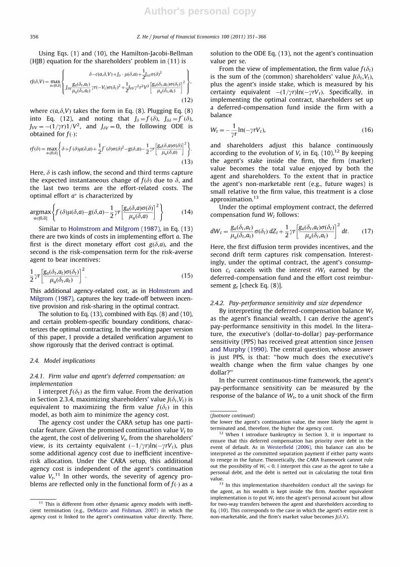
Using Eqs. (1) and (10), the Hamilton-Jacobi-Bellman(HJB) equation for the shareholders’ problem in (11) is

rJðd,VÞ ¼ maxa2½0,a �

d�cða,d,VÞþ Jd � mðd,aÞþ1

2JddsðdÞ2

JdVgaðdt ,atÞ

maðdt ,atÞgrð�VtÞsðdtÞ

2þ

1

2JVVg2r2V2 gaðdt ,atÞsðdtÞ

maðdt ,atÞ

� �2

8>>><>>>:

9>>>=>>>;

,

ð12Þ

where cða,d,VÞ takes the form in Eq. (8). Plugging Eq. (8)into Eq. (12), and noting that Jd ¼ f uðdÞ, Jdd ¼ f

00

ðdÞ,JVV ¼�ð1=grÞ1=V2, and JdV ¼ 0, the following ODE isobtained for f ð�Þ:

rf ðdÞ ¼ maxa2½0,a �

dþ f uðdÞmðd,aÞþ1

2f00

ðdÞsðdÞ2�gðd,aÞ�1

2gr

gaðd,aÞsðdÞmaðd,aÞ

� �2( )

:

ð13Þ

Here, d is cash inflow, the second and third terms capturethe expected instantaneous change of f ðdÞ due to d, andthe last two terms are the effort-related costs. Theoptimal effort a� is characterized by

argmaxa2½0,a �

f uðdÞmðd,aÞ�gðd,aÞ�1

2gr

gaðd,aÞsðdÞmaðd,aÞ

� �2( )

ð14Þ

Similar to Holmstrom and Milgrom (1987), in Eq. (13)there are two kinds of costs in implementing effort a. Thefirst is the direct monetary effort cost gðd,aÞ, and thesecond is the risk-compensation term for the risk-averseagent to bear incentives:

1

2gr

gaðdt ,atÞsðdtÞ

maðdt ,atÞ

� �2

: ð15Þ

This additional agency-related cost, as in Holmstrom andMilgrom (1987), captures the key trade-off between incen-tive provision and risk-sharing in the optimal contract.

The solution to Eq. (13), combined with Eqs. (8) and (10),and certain problem-specific boundary conditions, charac-terizes the optimal contracting. In the working paper versionof this paper, I provide a detailed verification argument toshow rigorously that the derived contract is optimal.

2.4. Model implications

2.4.1. Firm value and agent’s deferred compensation: an

implementation

I interpret f ðdtÞ as the firm value. From the derivationin Section 2.3.4, maximizing shareholders’ value Jðdt ,VtÞ isequivalent to maximizing the firm value f ðdtÞ in thismodel, as both aim to minimize the agency cost.

The agency cost under the CARA setup has one parti-cular feature. Given the promised continuation value Vt tothe agent, the cost of delivering Vt, from the shareholders’view, is its certainty equivalent ð�1=grÞlnð�grVtÞ, plussome additional agency cost due to inefficient incentive-risk allocation. Under the CARA setup, this additionalagency cost is independent of the agent’s continuationvalue Vt.

11 In other words, the severity of agency pro-blems are reflected only in the functional form of f ð�Þ as a

solution to the ODE Eq. (13), not the agent’s continuationvalue per se.

From the view of implementation, the firm value f ðdtÞ

is the sum of the (common) shareholders’ value Jðdt ,VtÞ,plus the agent’s inside stake, which is measured by hiscertainty equivalent �ð1=grÞlnð�grVtÞ. Specifically, inimplementing the optimal contract, shareholders set upa deferred-compensation fund inside the firm with abalance

Wt ¼�1

grlnð�grVtÞ, ð16Þ

and shareholders adjust this balance continuouslyaccording to the evolution of Vt in Eq. (10).12 By keepingthe agent’s stake inside the firm, the firm (market)value becomes the total value enjoyed by both theagent and shareholders. To the extent that in practicethe agent’s non-marketable rent (e.g., future wages) issmall relative to the firm value, this treatment is a closeapproximation.13

Under the optimal employment contract, the deferredcompensation fund Wt follows:

dWt ¼gaðdt ,atÞ

maðdt ,atÞsðdtÞ dZtþ

1

2gr

gaðdt ,atÞsðdtÞ

maðdt ,atÞ

� �2

dt: ð17Þ

Here, the first diffusion term provides incentives, and thesecond drift term captures risk compensation. Interest-ingly, under the optimal contract, the agent’s consump-tion ct cancels with the interest rWt earned by thedeferred-compensation fund and the effort cost reimbur-sement gt [check Eq. (8)].

2.4.2. Pay-performance sensitivity and size dependence

By interpreting the deferred-compensation balance Wt

as the agent’s financial wealth, I can derive the agent’spay-performance sensitivity in this model. In the litera-ture, the executive’s (dollar-to-dollar) pay-performancesensitivity (PPS) has received great attention since Jensenand Murphy (1990). The central question, whose answeris just PPS, is that: ‘‘how much does the executive’swealth change when the firm value changes by onedollar?’’

In the current continuous-time framework, the agent’spay-performance sensitivity can be measured by theresponse of the balance of Wt, to a unit shock of the firm

11 This is different from other dynamic agency models with ineffi-

cient termination (e.g., DeMarzo and Fishman, 2007) in which the

agency cost is linked to the agent’s continuation value directly. There,

(footnote continued)

the lower the agent’s continuation value, the more likely the agent is

terminated and, therefore, the higher the agency cost.12 When I introduce bankruptcy in Section 3, it is important to

ensure that this deferred compensation has priority over debt in the

event of default. As in Westerfield (2006), this balance can also be

interpreted as the committed separation payment if either party wants

to renege in the future. Theoretically, the CARA framework cannot rule

out the possibility of Wt o0. I interpret this case as the agent to take a

personal debt, and the debt is netted out in calculating the total firm

value.13 In this implementation shareholders conduct all the savings for

the agent, as his wealth is kept inside the firm. Another equivalent

implementation is to put Wt into the agent’s personal account but allow

for two-way transfers between the agent and shareholders according to

Eq. (10). This corresponds to the case in which the agent’s entire rent is

non-marketable, and the firm’s market value becomes Jðd,VÞ.

Z. He / Journal of Financial Economics 100 (2011) 351–366356

Author's personal copy

value.14 Specifically, by neglecting all drift terms, I have[recall that btðdt ,atÞ ¼ gaðdt ,atÞ=maðdt ,atÞ in Eq. (9)]

PPS¼dWt

df ðdtÞ¼

btðdt ,a�t ÞsðdtÞdZt

f uðdtÞsðdtÞdZt¼

btðdt ,a�t Þ

f uðdtÞ¼

gaðdt ,a�t Þ

maðdt ,a�t Þ

1

f uðdtÞ:

ð18Þ

Intuitively, PPS is the ratio between bt , which is theagent’s dollar incentive, and f uðdtÞ, which captures thevalue change (in dollars) of the firm. The optimal effort at

n

in Eq. (18) is endogenously determined by the optimiza-tion problem in Eq. (14).

The result in Eq. (18) implies that the agent’s pay-performance sensitivity depends on firm size dt . My latercalibration aims to replicate the well-known empiricalregularity that PPS is negatively related to firm size(e.g., Murphy, 1999).15 To this end, I now impose somestructure on my model to study the general pattern ofrelation between PPS and firm size.

When does PPS decrease with firm size? Suppose that

mðdt ,atÞ ¼ m0ðdtÞþatdm1t , sðdtÞ ¼ sds1

t ,

and gðdt ,atÞ ¼ g0ðdtÞþy2

a2t d

g1t ,

which imply that

maðdt ,atÞ ¼ dm1t and gaðdt ,atÞ ¼ yatd

g1t , ð19Þ

Here, m1, s1, y, and g1 are constants. This general speci-fication encompasses Baker and Hall (2004), who arguethat the effort impact on the firm growth (which I refer toas effort benefit) might be size-dependent, i.e., m140. Ifocus on m1, g1 and s1 which characterize the dependenceof the agent’s effort benefit, direct monetary effort cost,and indirect risk-compensation cost on firm size,respectively.

Given this structure, the first-order condition forEq. (14) (assuming an interior solution a�t ) is

f uðdÞdm1t �ya�t d

g1t �grs2y2a�t d

2ðg1þs1�m1Þ

t ¼ 0,

which implies the optimal effort as

a�t ¼f uðdÞdm1

t

ydg1t þgrs2y2d2ðg1þs1�m1Þ

t

: ð20Þ

Plugging Eqs. (19) and (20) into Eq. (18), one can showthat f uðdÞ cancels, and

PPS¼1

1þygrs2dg1þ2s1�2m1t

: ð21Þ

Therefore, the necessary and sufficient condition for anegative relation between PPS and firm size dt is

g1þ2s1�2m140: ð22Þ

In other words, when the size-dependence of the effortcost (either direct cost part g1 or indirect cost part s1) issufficiently large, or the size-dependence of effort benefitis sufficiently small, the firm should design an incentivecontract whose power is decreasing in firm size.

When I apply the optimal contracting results to theLeland framework in Section 3, I set

mðd,aÞ ¼ ðfþaÞd, sðdÞ ¼ sd, and gðd,aÞ ¼y2

a2d:

Here, g1 ¼ s1 ¼ m1 ¼ 1, and g1þ2s1�2m1 ¼ 1. Thereforethe PPS in the optimal contract is

PPS¼1

1þygrs2dt,

which is falling with firm size.Several attempts are made in the literature to estimate

these parameters. It is well known (as the leverage effect)that the large firm has a greater dollar variance but asmaller return variance, i.e., s1 2 ð0,1Þ. Cheung and Ng(1992) fit an EGARCH (exponential general autoregressiveconditional heteroskedasticity) model with CEV (constantelasticity of variance) specification to a large sample ofindividual stocks (as opposed to certain stock index,which is common in this literature) and find that s1 fallsin the range of 0.84 (in the 1960s) and 0.94 (in the1980s).16 This estimation is subject to the caveat that dt

is being approximated by the firm’s stock price. For m1

and g1, Baker and Hall (2004) assume that the agent’seffort cost is independent of firm size (i.e., g1 ¼ 0) and findthat m1 ¼ 0:4. If I instead set g1 ¼ 1, then one can showthat the effort benefit measure that Baker and Hall (2004)are estimating is effectively m1�0:5. Therefore, the esti-mate for m1 in my model (with g1 ¼ 1) is approximately0.9 (close to the choice of m1 ¼ 1 in Section 3). The bottomline is, the condition Eq. (22) that guarantees a negativerelation between PPS and firm size holds for theseestimates, which extends indirect support to my model.

CRRA (power) preference. My entire analysis hinges onthe assumption of CARA (constant-absolute-risk-aversion,exponential) preference, which implies that the agent’srisk absorbing capacity is independent of his wealthlevel. As an important ingredient for PPS, the risk absorb-ing capacity directly determines the risk compensationcost in Eq. (15), which in turn pins down the size-dependence of PPS in Eq. (21). What can we say if instead

14 Strictly speaking, in the executive compensation literature, the

pay-performance sensitivity is with respect to the shareholders’ value,

which should exclude the agent’s non-marketable stake. There are two

reasons that this treatment is inessential: (1) the magnitude of PPS is

small (125%), and (2) empirically, the executive’s PPS mainly comes

from his or her inside holdings, which are marketable. For other

definitions of performance sensitivities (e.g., pay-performance elastici-

ties) and an agency model distinct from the Holmstrom and Milgrom

(1987) framework, see Edmans, Gabaix, and Landier (2009).15 Typically, the PPS in executive compensation literature considers

only the chief executive officer’s incentive holdings. My model takes this

interpretation as well, so that the agent is the single top manager of the

firm. Readers can also interpret the manager here as a team of top

managers, and the relevant PPS measure becomes the inside holdings of

the firm’s officers and directors. Even though it is theoretically possible that

a larger firm might have more top managers who, as a team, hold more

inside shares, empirically the opposite holds. For instance, Holderness,

Kroszner, and Sheehan (1999) show a negative relation between the total

ownership of officers and directors and firm size.

16 One important determination of s1 is the correlation among the

projects taken by the firm. Conditional on firm size, s1 tends to be lower

for conglomerate firms (so the projects have diversified activities) than

specialized firms (so the projects are highly correlated), which suggests

different implications for PPS across these two types of firms. I thank the

referee Hayne Leland for this excellent point.

Z. He / Journal of Financial Economics 100 (2011) 351–366 357

Author's personal copy

the agent has a CRRA (constant relative risk aversion,power) preference?

Unfortunately, the wealth effect in the CRRA prefer-ence complicates the optimal contracting significantly,and not much is known about the solution to thatproblem.17 In the literature, several attempts are madeto accommodate this question. For example, Baker andHall (2004) solve a static optimal contracting problem asif the agent has an exponential utility. However, theyspecify the agent’s absolute risk aversion parametergðWtÞ ¼ g0=Wt (where g0 is a positive constant) to beproportional to the inverse of his wealth 1/Wt, as if theagent has a power utility. Here I take this simple approachas well.

It is important to note that the agent’s wealth Wt is notnecessarily proportional to firm size dt . Ideally I wouldlike to derive the path of Wt endogenously from themodel, but it is not available in CARA setting.18 Becausethe question at hand is a calibration question, I resort helpfrom data. Empirically, it is well known that, managers inlarger firms, although get higher pay in terms of dollaramounts, have lower inside stakes (Murphy, 1999). Mostof literature (e.g., Baker and Hall, 2004) use the manager’stotal compensation Compt to approximate his wealth Wt.In fact, Gabaix and Landier (2008) calibrate thatComptpd1=3

t , i.e., the elasticity between pay level andfirm size is 1/3. Given this result, I set the agent’s absoluterisk aversion parameter to be

gðWtÞ ¼ g0d�1=3t ,

where g0 is another positive constant potentially differentfrom g0. Plugging this result into Eq. (21) yields

PPS¼1

1þyg0rs2dg1þ2s1�2m1�1=3t

:

Therefore, under the CRRA preference, the necessary andsufficient condition that ensures a negative relationbetween PPS and firm size dt becomes

g1þ2s1�2m1413: ð23Þ

This condition holds for the case g1 ¼ s1 ¼ m1 ¼ 1 that isstudied in Section 3, as well as for the empirical estimatesof fg1,s1,m1g discussed in the previous subsection. Thus,even taking into account the fact that the agent mighthave a risk-aversion decreasing with his wealth (asimplied by CRRA preferences), my model has qualitativelysimilar predictions under reasonable parameterizations.

3. Revisiting Leland, 1994: optimal capital structure

This section applies the optimal contracting resultsderived in Section 2 to Leland (1994) with debt holders,and studies the interaction between dynamic compensa-tion and capital structure.

3.1. Model specification

Following Leland (1994), I consider the case that

ddt ¼ ðfþatÞdt dtþsdt dZt ,

where f and s are constants. In the language of Eq. (1),mðd,aÞ ¼ ðfþaÞd and sðdÞ ¼ sd. Here, f is the baselinegrowth level, and by exerting effort the agent can accel-erate the firm growth. The agent’s effort cost takes theform gðd,aÞ ¼ ðy=2Þa2d, which is quadratic in a and linearin size d.

Recall that in Section 2.1 I restrict the agent’s actionspace to a bounded interval ½0,a�, and the calibration inthe unlevered firm might call for a binding effort at ¼ a inthe optimal contract. In fact, under the parametrizationconsidered later, the first-best solution has aFB

t ¼ a. Tocharacterize the first-best solution, I simply set g¼ 0 inEq. (13) (so there is no agency problem), and, as a result,

rf FBðdÞ ¼ max

a2½0,a �dþ f FBuðdÞðfþaÞdþ

1

2f FB00 ðdÞs2d2

�y2

a2d� �

,

ð24Þ

where f FBðdÞ is the first-best firm value without agencyproblems. Because all model elements are proportional tod, I guess that f FBðdÞ ¼ AFBd, where AFB is a constant to besolved. Plugging into Eq. (24) yields

rAFB¼ max

a2½0,a �1þAFBðfþaÞ�

y2

a2

� �,

which jointly determines aFB and AFB. In the Appendix(Section A.3) I give the exact condition under which aFB

binds at a.Independent of whether aFB binds at a or not, the scale-

invariance of this model implies that, in the first-best case,the firm’s cash flow – as well as the firm value – follows ageometric Brownian motion. Due to its analytical conveni-ence, this setup has become the workhorse in the literatureof structural models of capital structure (e.g., Leland,1994; Goldstein, Ju, and Leland, 2001).

3.2. Optimal contracting in an unlevered firm

Before introducing debt into this framework, I applythe optimal contracting results obtained in Section 2 to anunlevered firm. To implement effort at, Eq. (9) implies thatthe agent’s incentive slope bt ¼ yat . Then Eq. (13)becomes

rf ðdÞ ¼ maxa2½0,a �

dþ f uðdtÞ � ðfþaÞdþ1

2f00

ðdtÞs2d2�y2

a2d�

�1

2gry2a2s2d2

�: ð25Þ

17 Edmans, Gabaix, Sadzik, and Sannikov (2009) consider a multi-

plicative effort cost model and impose some modification on the timing

structure to make the linear contract optimal in every instant. They

solve a long-term optimal contracting problem in closed-form if the

optimal contract aims to implement a maximum target effort (exogen-

ously given). In the optimal contract, the implemented effort is the

constant target effort level, and the return PPS (i.e., the log change of

manager’s compensation to the log change of firm value) is also a

constant independent of firm size.18 In the theoretical result with CARA preference, Wt in Eq. (17) can

be negative, which is inappropriate to define gðWtÞ ¼ g0=Wt .

Z. He / Journal of Financial Economics 100 (2011) 351–366358

Author's personal copy

Simple calculation yields the optimal effort as (the opti-mal effort might bind at a along the optimal path)19:

a�t ¼minf uðdtÞ

yð1þygrs2dtÞ,a

� �: ð26Þ

As discussed in Section 2.4.2, when the optimal effortlevel is interior, PPS is decreasing in firm size dt as

PPS¼1

1þygrs2dt, ð27Þ

Fundamentally, this result is due to the fact that, as thefirm grows, the quadratic risk-compensation cost12 gry2a2s2d2

t is in the order of d2t , while the incentive

benefit is in the order of dt [check Eq. (25); in theAppendix (Section A.5) I show that when dt-1,f uðdtÞ-1=ðr�fÞ]. This exactly reflects the common wis-dom that managers in larger firms have lower poweredincentive schemes due to risk considerations.20

Another appealing feature, which is closely related tothe pattern of PPS falling in firm size, is that the endo-genous firm growth rate fþa�t is decreasing in firm size dt

as well (see Section 3.4.3 for a numerical example). Thenegative relation between firm size and growth is studiedin, for instance, Cooley and Quadrini (2001). In this model,because incentivizing the agent is more costly in largerfirms, the optimal contract implements a lower effort inlarger firms, leading to a lower growth.

3.3. Optimal employment contract and leverage

3.3.1. Additional assumptions

Suppose that the firm issues debt to take advantage oftax shields. Relative to the standard bilateral contractingframework between investors (the principal) and theagent, now I have heterogenous investors—shareholdersand debt holders. To abstract from complicated contract-ing issues among three parties, I make the followingassumptions. First, the debt contract takes the formstudied in Leland (1994), i.e., only the consol bond (witha constant coupon rate C) is considered, and shareholders(with their perfectly aligned agent when they are dealingwith debt holders) can endogenously default when thefirm’s financial status deteriorates. Second, shareholders

can fulfill the promise of the agent’s continuation value atbankruptcy as a part of employment contract. In otherwords, when bankruptcy occurs, the agent is guaranteedwith the deferred-compensation fund W defined in Eq. (16).This assumption is commented upon in Section 3.4.2.

Another important timing assumption is that, in thismodel, shareholders design the employment contract asan optimal response to the leverage decision. Theoreti-cally, this is consistent with the fact that, in this CARAframework, a long-term optimal contract can be imple-mented by a sequence of short-term contracts (Fudenberg,Holmstrom, and Milgrom, 1990). Essentially, in the CARAframework studied here, shareholders and the agent canrevise the contract (as long as both parties agree to do so)once the debt is issued, which generates the debt-over-hang problem analyzed in Section 3.4.2.21

These assumptions represent a minimum, but essen-tial, departure from Leland (1994). They reflect the keyeconomic rationale regarding the manager’s objective incorporations in United States: Managers are supposed tobe responsible to shareholders only (Brealey, Myers, andAllen, 2006).

3.3.2. Equity value and endogenous default

Similar to the case of unlevered firms, the share-holders’ value function is JEðd,VÞ ¼ f EðdÞþð1=grÞlnð�grVÞ.The separability between d and V hinges on the assump-tion that in the leveraged firm the shareholders canalways keep the promise of delivering the continuationpayoff V to the agent, even when the firm goes bankruptat d¼ dB. In the implementation, the promise is guaran-teed by the deferred-compensation fund, which haspriority over debt in the event of bankruptcy.

As in Section 2.3.4, by writing down the HJB equationfor JEðd,VÞ, the following ODE is reached for the equityvalue f EðdÞ, where the control is over at and the bank-ruptcy boundary dB:

rf EðdÞ ¼ max

a2½0,a �,dB

d�Cð1�tÞþ f EuðdÞ � ðfþaÞdþ1

2f E00 ðdÞs2d2

�

�1

2ya2d�

1

2gry2a2s2d2

�, ð28Þ

where C is the coupon rate and t is the corporate tax rate.The equity value f EðdÞ is the sum of (common) share-holders’ value JEðd,VÞ and the agent’s deferred-compensa-tion fund �ð1=grÞlnð�grVÞ. Compared with Eq. (25)without debt, Eq. (28) has an additional cash outflowCð1�tÞ as the after-tax coupon payment. Similar toEq. (26), the optimal effort policy is

a�t ¼minf EuðdtÞ

yð1þygrs2dtÞ,a

� �: ð29Þ

Plugging it into Eq. (28) yields the ODE to characterize theoptimal contracting.

When dt falls to a certain level, say, dB, shareholdersrefuse to serve the coupon payment by simply declaring

19 When a binds at a , the same incentive loading bt ¼ ya applies:

Investors can set a higher incentive loading, but it is costly to do so

because the agent is risk-averse. And, because firm value is increasing in

the cash flow level d, one can formally show that in this model f uðdÞ is

always positive, therefore an never binds at zero. For formal proofs, see

the Appendix (Section A.4).20 For instance, (Murphy, 1999, p. 2531) states: ‘‘The inverse rela-

tion between company size and pay-performance sensitivities is not

surprising, since risk-averse and wealth-constrained CEOs of large firms

can feasibly own only a tiny fraction of the companyyThe result merely

underscores that increased agency problems are a cost of company size

that must weighed against the benefits of expanded scale and scope.’’ Of

course, this reasoning is precise when the manager’s risk-absorbing

capacity is independent of firm size, which holds only for CARA

preference. However, this statement is probably better interpreted as

following: Even though the managers in larger firms might have greater

risk-absorbing capacity (presumably because they receive higher pay),

their greater risk-absorbing capacity cannot offset the higher total risk in

larger firms. For a related discussion of CRRA preference, see Section

2.4.2.

21 In this CARA setting, the resulting optimal contract is renegotia-

tion-proof, as the Pareto boundary is always downward-sloping, i.e.,

JV ¼ 1=grV o0 (V is negative in this model).

Z. He / Journal of Financial Economics 100 (2011) 351–366 359

Author's personal copy

bankruptcy. This is captured by the value-matchingboundary condition

f EðdBÞ ¼ 0 ð30Þ

and the smooth-pasting condition

f EuðdBÞ ¼ 0: ð31Þ

Both conditions are standard in this literature (e.g., Leland,1994). These conditions are a result of maximizing theshareholders’ value JEðd,VÞ. But because these policies aretoward debt holders, it is equivalent to maximizing f EðdÞ,i.e., the joint (ex post) surplus enjoyed by shareholdersand the agent.22

For the boundary condition on the other end, when dt

takes a sufficiently large value d-1, the bankruptcyevent is negligible. In the Appendix (Section A.5) I showthat

f EðdÞC f ðdÞ�Cð1�tÞ

r, ð32Þ

where f ð�Þ captures the firm value under a Gordon growthmodel with a growth rate f [see Eq. (34)], and Cð1�tÞ=r isthe value for a perpetual after-tax coupon payment. Thenone can numerically solve for f Eð�Þ and dB, based onEq. (30)–(32). For detailed numerical methods, see theAppendix (Section A.5).

3.3.3. Debt value and capital structure

Given the implemented effort policy a�ðdÞ in Eq. (29),one can evaluate the consol bond with a promised couponrate C. Because debt holders anticipate the optimal con-tracting between shareholders and the agent, the value ofthe corporate debt, DðdÞ, satisfies

rDðdÞ ¼ CþDdðdÞ � ðfþa�ðdÞÞdþ12DddðdÞs2d2,

with DðdBÞ ¼ ð1�aÞf ðdBÞ, where ao1 is the percentagebankruptcy cost and DðdÞ-C=r as d-1. Here I simplyassume that, once bankruptcy occurs, debt holders paythe bankruptcy cost af ðdBÞ and then keep running theproject as an unlevered firm.23

Given the time-0 cash flow level d0, shareholderschoose coupon C to maximize the total levered firm valuef Eðd0;CÞþDðd0;CÞ before the debt issuance. They thendesign the optimal contract with an agent who has anoutside option v0. As discussed in Section 3.3.1, thistiming assumption is equivalent to allowing shareholdersand the agent to revise the employment contract ex postafter the debt issuance.

The firm’s optimal leverage ratio is defined as

LRðd0Þ �Dðd0;C

�ðd0ÞÞ

f Eðd0;C�ðd0ÞÞþDðd0;C�ðd0ÞÞ:

In Leland (1994), the scale-invariance implies that theoptimal leverage ratio LR is independent of firm size d0.However, in this model the quadratic risk-compensationeliminates the scale invariance. In fact, in the followingcalibration exercises, I mainly investigate the divergentleverage decisions for firms with different sizes.

3.3.4. Parameterization

Table 1 tabulates the baseline parametrization. Inter-est rate r¼ 5%, bankruptcy cost a¼ 25%, and tax ratet¼ 20% (considering personal tax effect) are typical in theliterature (e.g., Leland, 1998).

I also record the average growth rate in the 50-yearsimulation, and this measure helps pin down f and a. Inthe literature with constant coefficients, Goldstein, Ju, andLeland (2001) calibrate a slightly negative m, and Leland(1998) chooses the growth rate m¼ 1%. Under the choiceof f¼�0:5% and a ¼ 5% (a is irrelevant for levered firmsas the optimal effort fa�g never binds at 5%; see Fig. 2), thesimulated average growth rates fit these numberssquarely across various firm sizes (see Table 2).

Because in my calibration the optimal effort never bindsat a in levered firms, the pay-performance sensitivity is1=1þygrs2dt as in Eq. (27).24 Based on this result, I choosethe agency-related parameters [risk aversion g¼ 5 which isthe median value used in Haubrich (1994), and effort costy¼ 35] and the starting firm size d0 to match the PPSdocumented in the empirical literature. Jensen and Murphy(1990) report a PPS of 0:3% in their sample (1969–1983),while Hall and Liebman (1998) document a higher PPS withmean 2.5%. Aggarwal and Samwick (1999) control for thefirm risk and report a mean PPS of 6.94% from the ordinaryleast square regression. For the size-dependence pattern ofPPS, Murphy (1999) finds that for Standard & Poors 500firms, the PPS is approximately 1% for large firms, 1.5% forMidcap firms, and 3% for small firms. Hall and Liebman(1998) find a mean PPS around 2.5%, and in page 676 they

Table 1Baseline parameters.

Model parameters Parameter values

Risk aversion (g) 5

Effort cost (y) 35

Lower bound growth (f) �0.5%

Upper bound effort (a) 5%

Volatility (s) 25%

Interest rate (r) 5%

Bankruptcy cost (a) 25%

Marginal tax rate (t) 20%

I take volatility s¼ 25%, interest rate r¼ 5%, bankruptcy cost a¼ 25%,

and tax rate t¼ 20% from Leland (1998). I set g¼ 5 which is the median

value used in Haubrich (1994). The firm growth parameters f¼�0:5%

and a ¼ 5% are chosen to match the average firm growth rate used in the

literature. The effort cost y¼ 35 is set to (roughly) match the PPS

documented in the empirical literature.

22 This result implies that, despite the agency conflicts between the

agent and shareholders, under the optimal contract they have perfectly

aligned interests with respect to the policy toward debt holders. In other

words, the default policy does not depend on whether shareholders or

the agent is in charge of the bankruptcy decision. This differs

from Morellec (2004), in which the agent tends to keep the firm alive

longer for more private benefits.23 Also, the new agent’s outside option is v0 ¼�1=gr, so W0 ¼ 0. The

results in the paper are insensitive to the treatment of unlevered firm

after the bankruptcy.

24 The presence of debt does not affect the expression of PPS in

Eq. (27). To see this, the agent’s performance is measured as the change

of equity value f EðdÞ. However, f EuðdÞ cancels in Eq. (27) when the

optimal effort a�ðdÞ takes an interior solution [check the derivation in

Eq. (21)].

Z. He / Journal of Financial Economics 100 (2011) 351–366360

Author's personal copy

note that ‘‘the largest firms in our sample (market valueover $10 billion) have a median Jensen and Murphy statistic(PPS) that is more than an order of magnitude smaller thanthe smallest firms in our sample (market value less than$500 million).’’

3.4. Results and discussions

3.4.1. Optimal leverage ratio

Because debt-overhang adversely affects the firm’sendogenous growth, relative to Leland (1994) firms take

less leverage for their optimal capital structure in thismodel. Fig. 1 shows the optimal leverage ratio (the solidline) for firms with different sizes. For better comparison,Fig. 1 also provides two benchmark optimal leverageratios predicted by the Leland (1994) model, with exo-genous constant growth. The dashed line with circles(63.21%) is the first-best case, in which the cash flowgrowth rate is aþf¼ 4:5%. However, as in Section 3.2,the agency problem alone reduces the firm growth, whichwould lead to a lower leverage ratio even without debt-overhang. To address this issue, I take the results of

Table 2optimal capital structure for firms with different sizes.

Initial cash flow level (firm size) d0

50 100 150 200 250

Panel A: Optimal debt policies

Optimal coupon Cn 24.50 61.35 106.00 147.62 203.15

Default boundary dB 7.97 22.79 40.58 57.28 79.98

Scaled default boundary dB=d0 (percent) 15.95 22.79 27.05 28.64 31.99

Panel B: Valuation and leverage

Debt value Dðd0Þ 446.05 997.44 1640.02 2267.70 3090.52

Leverage ratioDðd0Þ

Dðd0Þþ f Eðd0Þ(percent)

39.35 47.70 53.57 56.10 61.32

Credit spreads (basis points) 49.22 115.12 146.34 150.98 157.34

Panel C: Simulation results

Average growth (percent) 1.95 0.50 0.12 �0.05 �0.17

Average volatility (percent) 25.04 24.98 25.04 25.03 25.01

Pay-performance sensitivity (percent) 5.33 2.52 1.69 1.29 0.99

The parameters are r¼ 5%, s¼ 25%, y¼ 35, g¼ 5, f¼�0:5%, a ¼ 5%, a¼ 25%, and t¼ 20%. Credit spreads are calculated as ðC=D�rÞ � 10,000. I simulate

the model for 50 years to obtain the average growth rate and volatility for dd=d, given the initial d0. I also calculate the agent’s average pay-performance

sensitivity based on Eq. (27).

50 100 150 200 2500.35

0.4

0.45

0.5

0.55

0.6

0.65

0.7

Inital cashflow level (firm size) δ0

Optimal leverage ratio

with agency and debt-overhangLeland (1994): first-best coefficientsLeland (1994): (simulated) coefficients without debt

Fig. 1. Optimal leverage ratio as a function of initial cash flow level (firm size). I plot the two benchmark leverage ratios under Leland (1994). The first

one is based on the first-best coefficients (m¼ 4:5% and s¼ 25%), which gives a leverage ratio 63.21% plotted in the dashed line with circles. The second

one is based on the time series averages in simulating the unlevered firm in Section 3.2 (m¼ 3:31% and s¼ 25:02%; for simulation details, see Footnote

25). This case yields a leverage ratio 61.59% plotted in the dotted line with asterisks. The parameters are r¼ 5%, s¼ 25%, y¼ 35, g¼ 5, f¼�0:5%,

a ¼ 5%, a¼ 25%, and t¼ 20%.

Z. He / Journal of Financial Economics 100 (2011) 351–366 361

Author's personal copy

unlevered firms from Section 3.2, simulate the model, andobtain time series averages of the cash flow growth andvolatility.25 I then use these estimates as inputs tocalculate the Leland leverage ratio, which is graphed inthe dotted line with asterisks (61.59%) in Fig. 1.

The optimal leverage ratios are reported in Table 2along with other measures. For each initial cash flow leveld0, I calculate the sample mean of growth and volatility ofdd=d over one hundred years in five hundred simulations(see Panel C in Table 1). I also report the sample average ofpay-performance sensitivity based on Eq. (27); thesenumbers fit the empirical estimates discussed in Sec-tion 3.3.4 squarely. For small firms (d0 ¼ 50), the optimalleverage ratio falls from 61:59% (or 63.21% in the first-bestcase) to 39.35%.26 In contrast, the optimal leverage ratiofor large firms is close to the result under Leland (1994).I will come back to this cross-sectional result shortly.

3.4.2. Debt-overhang

In Fig. 1, the optimal leverage ratio is lower relativeto Leland (1994). The reason is debt-overhang, where Iinterpret the agent’s effort as a form of investment;see Hennessy (2004) for a similar mechanism. In mymodel, shareholders design an employment contract tomaximize the ex post equity value, and the smooth-pasting condition Eq. (31) implies that f EuðdÞ goes to zeroas d approaches the default boundary dB. It implies that,once the firm is close to bankruptcy, shareholders gainalmost nothing by improving the firm’s performance.Then, according to Eq. (29) which says that the optimaleffort an is proportional to f EuðdÞ, shareholders implementdiminishing effort (through providing diminishing incen-tives) during financial distress. As a result, in addition tothe traditional bankruptcy cost, in this model the debtbears another form of cost due to debt-overhang.

This mechanism is illustrated in Fig. 2. The left panelplots the implemented effort investment an in solid line as afunction of firm’s financial status d for small firms (d0 ¼ 50).As explained shortly, the debt-overhang problem is moresevere for small firms. I also plot the optimal effort policywithout debt-overhang (the dashed line), which corre-sponds to the case of unlevered firms studied in Section 3.2.

Relative to the effort policy without debt-overhangplotted in the dotted line, an abrupt drop of implementedeffort is evident when the firm is in the verge of bank-ruptcy (d-dB ¼ 7:97). From the view of social welfare, inthis situation a higher effort is desirable, because it helpsavoid the costly bankruptcy once d hits dB. However, it isnot in the shareholders’ interest to ask the agent to workhard. When the firm approaches bankruptcy, share-holders obtain zero marginal value from improving d.Consequently, they implement diminishing effort, atypical symptom of debt-overhang.

It is worth emphasizing that the driving forces of thedebt-overhang result are the endogenous nature of firmgrowth, and the smooth-pasting condition of the share-holders’ value; both ingredients are generic in practice.

10 20 30 40 50 60-0.01

0

0.01

0.02

0.03

0.04

0.05

Cash flow level (firm size) δ

Implemented effort a* for δ0 =50 (small firms)

100 150 200 250 300-0.01

0

0.01

0.02

0.03

0.04

0.05

Cash flow level (firm size) δ

Implemented effort a* for δ0 =250 (large firms)

With debt-overhangWithout debt-overhang

With debt-overhangWithout debt-overhang

δB=7.97 with δ

0=50 δB=79.98 with δ0=250

Fig. 2. Implemented effort policies with debt-overhang for small (d0 ¼ 50) and large (d0 ¼ 250) firms under optimal leverage decisions. The optimal effort

policy a�ðdÞ with debt-overhang is shown in the solid line, and the optimal effort policy in an unlevered firm without debt-overhang is shown in dashed

line. I also mark the optimal endogenous default boundary, where shareholders optimally (ex post) default and implement a zero effort. The parameters

are r¼ 5%, s¼ 25%, y¼ 35, g¼ 5, f¼�0:5%, a ¼ 5%, a¼ 25%, and t¼ 20%.

25 Specifically, to match the relevant range for d in levered firms, I

set the initial d0 ¼ 250 and stop the process once d reaches 7.97 (which

is the lowest default boundary in the calibration). Also, the simulation

length is 50 years to mitigate the impact of initial condition. I then

average the time series mean of growth rate and volatility across five

hundred simulations, which gives an average growth rate (volatility) as

3.31% (25.02%). Other treatment gives similar results.26 This reduction is comparable to other modifications of the Leland

(1994) benchmark. For instance, by combining both the ‘‘callable’’ feature

of the debt and upward capital restructuring together, Goldstein, Ju, and

Leland (2001) reduce the optimal leverage from 49.8% to 37.1% in their

baseline case.

It is not easy to accommodate the dynamic capital restructuring into

my framework, as this model does not have the convenient scale-

invariance property. Certainly, as in Goldstein, Ju, and Leland (2001),

the possibility of raising leverage in the future should reduce the firm’s

initial leverage. In fact, dynamic capital restructuring would have an

interesting impact to this model if the restructuring was downward, i.e.,

reducing debt when the firm’s cash flow level drops. This is because in

this model almost all the action is on the downside where debt overhang

cuts down the efficient effort. If I only allow for upward restructuring as

in Goldstein, Ju, and Leland (2001), the interaction effect should be small.

Z. He / Journal of Financial Economics 100 (2011) 351–366362

Author's personal copy

Therefore, if in reality the management gives place toexisting shareholders (such as the board) during financialdistress, then debt-overhang is still present without theintermediate link of diminishing management incentives.

Leverage versus management incentives. The debt-over-hang generates a negative relation between leverage andagent’s working incentives. This result contrasts toCadenillas, Cvitanic, and Zapatero (2004), in which thelog agent’s compensation space is restricted to equityshares, and shareholders commit to this compensationscheme. In comparison, in this optimal dynamic contract-ing setup, I do not place any restriction on the contractingspace, and I allow for dynamically revising the employ-ment contract between the agent and shareholders.Finally, as discussed in Section 3.3.1, part of the imple-mentation of the optimal contract requires the firm to setthe agent’s deferred compensation aside as cash. Thisway, shareholders commit to fully insulate the agent’scompensation from bankruptcy. I now discuss theseassumptions by relating them to ‘‘inside debt’’ investi-gated in Sundaram and Yermack (2007).

Inside debt. Several interesting remarks can be maderegarding the above assumptions, which point to therobustness of the debt-overhang result. First, in reality,although there are certain revising activities such as reset-ting the strike price of executives’ previously awardedoptions, modifying compensation contract is not friction-less. For instance, managers’ pensions – as a form ofdeferred compensation – are calculated according to certainprespecified formulae. More importantly, these pensionsrepresent unsecured, unfunded debt claims against firmassets (inside debt as advocated in Sundaram and Yermack,2007, and Edmans and Liu, 2011),27 which is not a seniorclaim against a cash-based deferred compensation fund asin my implementation. As a result, this portion of compen-sation scheme can potentially alleviate the debt-overhangproblem in this paper and the risk-shifting problemin Edmans and Liu (2011).28

Nevertheless, for inside debt to work, one also needsshareholders’ and the agent’s commitment on other com-pensation schemes to prohibit undoing the inside debt. Theimportant point is that, to rule out ex post revising, share-holders and the agent need commitment with debt holderson all compensation schemes, not on one or some schemes.Put differently, as long as shareholders can modify theresidual compensation freely, they can still undo the insidedebt, and theoretically return to the optimal contract without

commitment. This implies that my theoretical results arerobust to the practice of inside debt. In addition, someindirect empirical evidence (Bryan, Hwang, and Lilien,2000) is consistent with this view of ‘‘undoing’’ or ‘‘dynami-cally revising’’ the employment contract, which can be apotential topic for future empirical studies.29

3.4.3. Size-heterogeneity

My model offers another explanation why small firmstake less leverage relative to their large peers, a stylizedfact documented in the literature (e.g., Frank and Goyal,2005). The mechanism here is rooted in divergent seve-rities of the aforementioned debt-overhang problem fordifferent size firms. In this model, to be consistent withthe inverse relation between PPS and firm size, largerfirms implement lower effort. This implies that, for largerfirms, debt-overhang – which reduces the profitable effortinvestment – is less of concern. Consequently, larger firmsissue more debt to maximize the ex ante firm value.

This point is illustrated in the right panel in Fig. 2,where effort policies are plotted with and without debt-overhang for large firms (d0 ¼ 250). For better compar-ison, the right panel adopts the same scale as the leftpanel where small firms are considered. Debt-overhang ismoderate for large firms. As shown, at their relativelyhigh default boundary dB ¼ 79:98, the optimal effort evenwithout debt-overhang is low (only about 1.14%). There-fore, the drop of at

nwhen larger firms approach bank-

ruptcy – the exact force of debt-overhang – is lessdramatic compared with smaller firms (the left panel).In sum, in smaller firms the debt-overhang cost is greater,leading to a lower predicted leverage ratio.

It is important to add that this result is not driven byCARA preference. Instead, CARA preference is used only asthe analytical tool to match the empirical pattern of pay-performance sensitivity, and it is the negative relationshipbetween PPS and firm size that implies lower debt-over-hang costs in large firms.

3.4.4. Default policy and credit spreads

Table 2 also reports the endogenous default policies.The scaled default boundary dB=d0 are lower (so share-holders default later) than the Leland (1994) bench-mark.30 The intuition for shareholders to postponebankruptcy is as follows. In this model, a firm with recent

27 This means that when the firm becomes insolvent, pension

beneficiaries have the same priority as other unsecured creditors.

However, footnote 10 in Sundaram and Yermack (2007) gives an

example of the ‘‘secular’’ trust fund, which secures an executive’s

pension in a bankruptcy-proof form.28 These papers are closely related to the early theoretical work

by John and John (1993) who consider a risk-shifting problem. Essen-

tially, for the agent to maximize the firm’s value, the compensation

should be less aligned with shareholders when the leverage is higher,

which predicts a negative relation between leverage and PPS. There,

commitment is also essential, even though it appears not so in a two-

period model. In contrast, in this model, the agent is always perfectly

aligned with shareholders in terms of incentives thanks to potential

revising.

29 Bryan, Hwang, and Lilien (2000) analyze the Incentive-Intensity

(the change in the value of annual stock-based compensation per change

in equity value) and Mix (ratio of the value of annual stock-based

compensation to cash compensation) measures, which are based on the

annual stock-based grants only (as opposed to cumulative inside

holdings that relate to the agent’s wealth). They find that both Incen-

tive-Intensity and Mix decrease with firm leverage. Under the debt-

overhang framework studied in this paper, to the extent that working

incentives generated by inside debt is increasing with leverage, these

empirical results are consistent with the dynamic revising activity. Also,

decreasing Mix with leverage implies that financially troubled firms pay

the agent more cash compensation, a result consistent with my model if

the juniority of pensions force the firm to start paying out deferred

compensation to the agent by cash.30 For the Leland (1994) exogenous growth model, dB=d0 ¼ 39:73%

in the first-best parametrization, and dB=d0 ¼ 37:24% in the unlevered

firm parametrization.

Z. He / Journal of Financial Economics 100 (2011) 351–366 363

Author's personal copy

unsatisfactory performances has a lower cash flow level,or smaller size. But given a smaller risk-compensation,shareholders find it cheaper to motivate the agent, whichgives them more value to wait for future improvement.Because of the delayed default, my model producessimilar, but slightly lower, credit spreads (Panel Bin Table 2) than Leland (1994), conditional on comparableleverages.31

There are various theoretical models in which agencyproblems are countercyclical (e.g., Bernanke and Gertler,1989; Eisfeldt and Rampini, 2008, etc.). Acknowledgingthat the agency issue becomes more severe in recessions(for instance, a higher cash flow volatility or a higherconstant absolute risk aversion when the agent’s wealth islower), it is interesting to further explore the impact ofagency problems on credit spreads. Chen, Collin-Dufresneand Goldstein (2009) argue that the key mechanism inexplaining the high credit spread puzzle is that firmsdefault more frequently in those higher risk premiumstates. This countercyclical default policy might be relatedto exacerbated agency issues in these bad states, becausesevere agency frictions can lead to a great reduction inshareholder’ value of keeping the firm under their control.For instance, consider small firms d0 ¼ 50. By raising theagent’s constant absolute risk aversion coefficient g from5 to 10, while fixing coupon level C ¼ 24:50, the defaultboundary increases from 7.97 to 8.92, and as a result thecredit spread goes up substantially (49 bps versus 85 bps).I leave this for future research.

3.4.5. Asset volatility and leverage effect

Various empirical studies find that equity returnsbecome more volatile as the firm approaches bankruptcy.This phenomenon can be explained by the so-calledleverage effect, even holding the volatility of the under-lying asset constant.

In this model, the state variable for a firm’s financialstatus is its cash flow level, and I also assume a constantinstantaneous (return) volatility in the continuous-timesetup. However, when the sampling frequency cannot bearbitrarily high, the estimated variance differs from theinstantaneous volatility. Because of the hump-shapedendogenous effort (see Fig. 2), this model generateshigher conditional variances (based on infrequent sam-pling) when firms are in financial distress.

The mechanism is as follows. Due to debt-overhang,the firm’s endogenous growth is positively correlatedwith underlying performance shocks in financial distress.To see this, consider the implemented effort policy in theleft panel in Fig. 2. When d is close to dB ¼ 7:97, a�ðdÞ isincreasing in d. Then, a positive shock to d, by reducingdebt-overhang, gives rise to a higher effort a�ðdÞ. Thisfurther leads to a higher cash flow growth rate a�ðdÞþfand, in turn, magnifies the positive shock. Therefore,when sampling is infrequent, the observed return volati-lity is higher than the constant volatility s¼ 25%. For

instance, when d¼ 15, over one year the annualizedvolatility based on monthly observed data is about25.12%. When d is far away from the bankruptcy thresh-old, a�ðdÞ is decreasing in d, and the exact opposite forceleads to a lower volatility estimate (when d¼ 50, theabove mentioned annualized volatility is about 24.68%).

In sum, for a firm near bankruptcy, its financial statusbecomes more sensitive to underlying performanceshocks. In fact, this general message does not depend onthe discrete-sampling, as in this model the firm value(rather than the instantaneous cash flow rate) displays ahigher instantaneous volatility during financial distress.32

3.4.6. Debt covenants

A commonly observed debt covenant is that debtholders can force shareholders to go bankrupt whenthe firm’s cash flow d hits a prespecified level db

B. Thiscovenant is along the same line as ‘‘positive net-worthcovenants for protected debt’’ in Leland (1994) whichstipulates that the firm defaults whenever the asset valuedrops to the debt face value. Under the current cash flowframework, this can also be interpreted as a hard cove-nant on the interest coverage ratio, which, combined withcoupon C, gives the bankruptcy threshold.33

In the standard trade-off model as in Leland (1994), aforced earlier default always hurts firm value, because anearlier default reduces the tax benefit and raises thebankruptcy cost. In fact, if equity holders can fully commitin Leland (1994), then no default is the first-best outcome.

In contrast, due to the debt-overhang problem, in mymodel specifying db

B4dB might be welfare improving. Thereason is that, now around db

B, there is no longer smooth-pasting condition as in (31), and shareholders benefit fromimproving the firm performance. Then, specifying db

B4dB isequivalent to committing to provide incentives (to the agent)even in the deep financial distress, and it might be sociallyoptimal to do so. For instance, for small firms d0 ¼ 50, giventhe coupon C ¼ 24:50, the optimal db

B ¼ 8:054dB ¼ 7:97,and the firm value becomes 1133:8141133:67. Thoughsmall magnitude, this interesting finding distinguishes thismodel from Leland (1994) and its variations where the firmgrowth is exogenously specified.

4. Concluding remarks

By generalizing the optimal contracting result towidely used cash flow setups in finance, this paper offersa more tractable framework to investigate the impact ofagency problems in various economic contexts. Theabsence of wealth effect due to CARA preference simplifiesthe optimal contracting problem with private savings, and

31 For instance, based on the growth and the volatility estimates

(Panel C) of medium-size firms (d0 ¼ 150), under Leland (1994) a 53.57%

of leverage ratio translates into a credit spread of 175 basis points (bps),

which is higher than 146 bps in my model.

32 The firm’s asset value, generated by future cash flows, can be

defined as XðdtÞ ¼ Et ½R tðd ¼ dB Þ

t e�rðs�tÞds dsþ f ðdBÞ�, where tðd¼ dBÞ is the

first passage time of d hitting dB . Then, the instantaneous return

volatility of XðdtÞ is larger when dt is close to dB. The reason is that

XðdtÞ takes into account the impact on the stochastic growth m, which

positively correlates with dt during distress.33 Because part of the coupon C can be interpreted as constant

operating cost (in other words, the leverage derived here includes

operating leverage, too), the effective interest coverage ratio can be

much higher than implied by dbB=C.

Z. He / Journal of Financial Economics 100 (2011) 351–366364

Author's personal copy

I characterize the optimal contract by an ODE. Whenapplying my results to Leland (1994), I find that theunderinvestment of effort due to debt-overhang producesa lower optimal leverage ratio, and the interesting inter-action between agency issue and debt-overhang leadssmaller firms to take less debt in their leverage decisions.

The relatively simple structure in this paper leavesseveral directions for future research. For instance, incorpor-ating investment decisions would be desirable, as one canexplore the investment distortion and its interaction withfinancing decisions under agency problems. Also, incorpor-ating time-varying risk premia that is correlated with agencyfrictions (e.g., time-varying risk-aversion) is valuable toinvestigate the agency impacts on credit spreads.

Appendix A

A.1. Proof of Lemma 2

Consider any contract P¼ fc; ag that induces an opti-mal policy fc; ag from the agent with a value V 0. Theagent’s budget equation yields

St ¼

Z t

0erðt�sÞðcs�c sÞ ds,

which gives the agent’s optimal savings path, with thetransversality condition limT-1E½e

�rT ST � ¼ 0. The trans-versality condition holds for all measures induced by anyfeasible effort policies.

By invoking the replication argument similar to reve-lation principle, I consider giving the agent a directcontract P ¼ fc; ag, and shareholders have the same costto deliver this contract as P¼ fc; ag. Clearly taking con-sumption-effort policy fc; ag is feasible for the agentwithout private savings. I need to show that fc; ag isoptimal for the agent. Suppose that given the contractP, the agent finds that fcu; aug yields a strictly higherpayoff V0u 4 V 0 in problem (2), with associated savingspath

Stu ¼

Z t

0erðt�sÞðc s�csuÞ ds,

which satisfies transversality condition. However, con-sider the following saving path

St00 ¼ StþStu¼

Z t

0erðt�sÞðcs�csuÞds,

which also satisfies the transversality condition. But thisimplies that, given the original contract P, the saving ruleSt00 supports fcu; aug but delivering a strictly higher payoff

V0u. This contradicts with the optimality of fc ; ag under thecontract P.

A.2. Proof of Lemma 3

Given any savings St ¼ S and a contract P¼ fc; ag, fromtime-t on the agent’s problem is [recall Eq. (2)]

maxfc sg,fa sg

E

Z 1t�

1

g e�gðc s�gðds ,a sÞÞ�rðs�tÞ ds

� �ð33Þ

s:t: dSs ¼ rSs dsþcs ds�c s ds, St ¼ S, s4t

dds ¼ mðds,asÞ dsþsðdsÞ dZs:

Denote by fc�

s ,a�

s g the solution to the above problem, andby VtðP,SÞ the resulting agent’s value.

Now consider the problem with S¼ 0, which is thecontinuation payoff along the equilibrium path:

maxfc sg,fa sg

E

Z 1t�

1

g e�gðc s�gðds ,a sÞÞ�rðs�tÞ ds

� �s:t: dSs ¼ rSs dsþcs ds�c s ds, St ¼ 0, s4t

dds ¼ mðds,asÞ dsþsðdsÞ dZs:

I claim that the solution to this problem is fc�

s�rS,a�

s g, andtherefore the value is VtðP,0Þ ¼ egrSVtðP,SÞ. There are twosteps to show this. First, this solution is feasible. Second,suppose that there exists another policy fc su ,asu g that issuperior to fc

�

s�rS,a�

s g, so that the associated valueVtuðP,0Þ4e�grSVtðP,SÞ. Consider fc suþrS,asu g, which is fea-sible to the problem in (33). But under this plan theagent’s objective is

e�grS �maxEt

Z 1t�

1

ge�gðc su�gðds ,a su ÞÞ�rðs�tÞ ds

� �¼ e�grSVtuðP,0Þ4VtðP,SÞ,

which contradicts with the optimality of fc�

s ,a�

s g. As aresult, VtðP,SÞ ¼ e�grSVtðP,0Þ.

A.3. Subsection 3.1

Note that rAFB¼maxa2½0,a �f1þAFBðfþaÞ�ðy=2Þa2g, and I

am interested in characterizing the condition for the first-

best effort aFB to bind at a. When a takes an interior solution,

then a� ¼ AFB=y, and AFB ¼ 2=ðr�fþffiffiffiffiffiffiffiffiffiffiffiffiffiffiffiffiffiffiffiffiffiffiffiffiffiffiffiðr�fÞ2�2=y

qÞ. First, I

need to ensure that ðr�fÞ242=y so that AFB is real. Other-wise, the firm value is unbounded, resulting in an unbounded

aFB. Therefore, when ðr�fÞ2r2=y, aFBt ¼ a. Second, even

when ðr�fÞ242=y, it is possible that the implied the first-

best effort ð1=yÞ2=ðr�fþffiffiffiffiffiffiffiffiffiffiffiffiffiffiffiffiffiffiffiffiffiffiffiffiffiffiffiðr�fÞ2�2=y

qÞ4a. In this case,

the first-best effort also binds at aFBt ¼ a. Under both scenar-

ios, AFB ¼ ð1�ðy=2Þa2Þ=ðr�f�aÞ.

A.4. Subsection 3.2

Under the boundary conditions specified in Section3.2, f u is always positive in Eq. (25), therefore an neverbinds at zero in this problem. To see this, clearly f uð0Þ40[notice f ð0Þ ¼ 0, and for d40, even with zero effort (sowithout the agent) the value is positive]. When d-1,using Eqs. (25) and (26) one can check that

f ðdÞC f ðdÞ �1

r�fdþ

1

2ðr�fÞ2y2grs2: ð34Þ

which is increasing in d. Now suppose that there existsd140 such that f uðd1Þ ¼ 0. Take the smallest one so thatf00

ðd1Þo0 (i.e., f has to be concave on d1). Therefore,rf ðd1Þ ¼ d1þ

12 f00

ðd1Þs2d21od1. But there must exist

another point d24d1, such that f is deceasing in ½d1,d2�,and f becomes increasing again after d2 (as f is increasingwhen d is large enough). This implies f ðd2Þo f ðd1Þ,

Z. He / Journal of Financial Economics 100 (2011) 351–366 365

Author's personal copy

f uðd2Þ ¼ 0 and f00

ðd2Þ40. However, Eq. (25) implies thatrf ðd2Þ4d24d14rf ðd1Þ, a contradiction with f ðd2Þo f ðd1Þ.

A.5. Subsection 3.3.2

When d-1, the probability of bankruptcy is negligi-ble, and the firm value can be viewed as the unleveredfirm value minus the present value of after-tax couponpayment. Eq. (34) gives the unlevered firm value f whend-1, and f u approaches to 1=ðr�fÞ similar to thestandard Gordon growth model. Therefore f EðdÞC f ðdÞ�ð1�tÞC=r when d is sufficiently large.

I use Matlab built-in solver bvp4c to solve the model,setting the tolerance level to be 10�8. I set d ¼ 500. Insolving for the bankruptcy boundary dB, I first choose onecandidate d1

B and solve fE based on Eqs. (30)–(32) usingbvp4c. Then I evaluate f Euðd1

BÞ. If f Euðd1BÞ4(o)0 which

means that d1B is too low (high), I adjust d1

B upward(downward) to, say, d2

B. I use a bisection method to searchfor dB, which converges quickly.

References

Aggarwal, R., Samwick, A., 1999. The other side of the tradeoff: theimpact of risk on executive compensation. Journal of PoliticalEconomy 107, 65–105.

Baker, G., Hall, B., 2004. CEO incentives and firm size. Journal of LaborEconomics 22, 767–798.

Bernanke, B., Gertler, M., 1989. Agency costs, net worth, and businessfluctuations. American Economic Review 79, 14–31.

Biais, B., Mariotti, T., Plantin, G., Rochet, J., 2007. Dynamic securitydesign: convergence to continuous time and asset pricing implica-tions. Review of Economic Studies 74, 345–390.

Brealey, R., Myers, S., Allen, F., 2006. Principles of Corporate Finance,eighth ed. McGraw-Hill/Irwin, New York.

Bryan, S., Hwang, L., Lilien, S., 2000. CEO stock-based compensation: anempirical analysis of incentive-intensity, relative mix, and economicdeterminants. Journal of Business 73, 661–693.

Cadenillas, A., Cvitanic, J., Zapatero, F., 2004. Leverage decision andmanager compensation with choice of effort and volatility. Journal ofFinancial Economics 73, 71–92.

Chen, L., Collin-Dufresne, P., Goldstein, R., 2009. On the relation betweenthe credit spread puzzle and the equity premium puzzle, Review ofFinancial Studies, 22, 3367–3409.

Cheung, Y., Ng, L., 1992. Stock price dynamics and firm size: an empiricalinvestigation. Journal of Finance 47, 1985–1997.

Cooley, T., Quadrini, V., 2001. Financial markets and firm dynamics.American Economic Review 91, 1286–1310.

DeMarzo, P., Fishman, M., 2007. Optimal long-term financial contracting.Review of Financial Studies 20, 2079–2128.

DeMarzo, P., Sannikov, Y., 2006. Optimal security design and dynamiccapital structure in a continuous-time agency model. Journal ofFinance 61, 2681–2724.

Edmans, E., Liu, Q., 2011. Inside debt. Review of Finance 15, 75–102.Edmans, A., Gabaix, X., Landier, A., 2009. A multiplicative model of

optimal CEO incentives in market equilibrium. Review of FinancialStudies 22, 4881–4917.

Edmans, A., Gabaix, X., Sadzik,T., Sannikov, Y., 2009. Dynamic incentiveaccounts. Unpublished working paper, University of Pennsylvania,Wharton school, New York University, and Princeton University.

Eisfeldt, A., Rampini, A., 2008. Managerial incentives, capital reallocation,and the business cycle. Journal of Financial Economics 87, 177–199.

Frank, M., Goyal, V., 2005. Trade-off and pecking order theoriesof debt. In: Eckbo, B. (Ed.), Handbook of Corporate Finance:Empirical Corporate Finance. Elsevier/North-holland, Amsterdam,pp. 136–206 (Chapter 7).

Fudenberg, D., Holmstrom, B., Milgrom, P., 1990. Short-term contractsand long-term agency relationships. Journal of Economic Theory 51,1–31.

Gabaix, X., Landier, A., 2008. Why has CEO pay increased so much?Quarterly Journal of Economics 123, 49–100.

Goldstein, R., Ju, N., Leland, H., 2001. An EBIT-based model of dynamiccapital structure. Journal of Business 74, 483–512.

Hall, B., Liebman, J., 1998. Are CEOs really paid like bureaucrats?Quarterly Journal of Economics 113, 653–691.

Haubrich, J., 1994. Risk aversion, performance pay, and the principal-agent problem. Journal of Political Economy 102, 258–276.

He, Z., 2009. Optimal executive compensation when firm size followsgeometric Brownian motion. Review of Financial Studies 22,859–892.

He, Z., 2010. Dynamic compensation contracts with private savings.Unpublished working paper, University of Chicago, Booth School ofBusiness.

Hennessy, C., 2004. Tobin’s Q, debt overhang, and investment. Journal ofFinance 59, 1717–1742.

Holderness, C., Kroszner, R., Sheehan, D., 1999. Were the gold old daysthat good? Changes in managerial stock ownership since the greatdepression. Journal of Finance 54, 435–469.

Holmstrom, B., Milgrom, P., 1987. Aggregation and linearity in theprovision of intertemporal incentives. Econometrica 55, 303–328.

Jensen, M., Murphy, K., 1990. Performance pay and top-managementincentives. Journal of Political Economy 98, 225–264.

John, T., John, K., 1993. Top-management compensation and capitalstructure. Journal of Finance 48, 949–974.

Kocherlakota, N., 2004. Figuring out the impact of hidden savings onoptimal unemployment insurance. Review of Economic Dynamics 7,541–554.

Leland, H., 1994. Corporate debt value, bond covenants, and optimalcapital structure. Journal of Finance 49, 1213–1252.

Leland, H., 1998. Agency costs, risk management, and capital structure.Journal of Finance 53, 1213–1243.

Morellec, E., 2004. Can managerial discretion explain observed leverageratios? Review of Financial Studies 17, 257–294

Murphy, K., 1999. Executive compensation. In: Ashenfelter, O., Card, D.(Eds.), Handbook of Labor Economics. Elsevier/North-holland,Amsterdam, pp. 2485–2563 (Chapter 38).

Piskorski, T., Tchistyi, A., 2010. Optimal mortgage design. Review ofFinancial Studies 23, 3098–3140.

Rogerson, W., 1985. Repeated moral hazard. Econometrica 53, 69–76.Sannikov, Y., 2008. A continuous-time version of the principal-agent

problem. Review of Economic Studies 75, 957–984.Schattler, H., Sung, J., 1993. The first-order approach to the continuous-

time principal-agent problem with exponential utility. Journal ofEconomic Theory 61, 331–371.

Sundaram, R., Yermack, D., 2007. Pay me later: inside debt and its role inmanagerial compensation. Journal of Finance 62, 1551–1587.

Westerfield, M., 2006. Dynamic contracts with hidden actions in con-tinuous time. Unpublished working paper, University of SouthernCalifornia.

Williams, N., 2006. On dynamic principal-agent problems in continuoustime. Unpublished working paper, University of Wisconsin-Madison.

Z. He / Journal of Financial Economics 100 (2011) 351–366366