Journal of Business Valuation and Economic Loss Analysis · Volume 5, Issue 1 2010 Article 7 Journal of Business Valuation and Economic Loss Analysis Fundamentals of Functional Business

Volume 5, Issue 1 2010 Article 7

Journal of Business Valuation andEconomic Loss Analysis

Fundamentals of Functional BusinessValuation

Manfred Jürgen Matschke, Ernst-Moritz-Arndt-UniversitätGerrit Brösel, Technische Universität Ilmenau

Xenia Matschke, Universität Trier

Recommended Citation:Matschke, Manfred Jürgen; Brösel, Gerrit; and Matschke, Xenia (2010) "Fundamentals ofFunctional Business Valuation," Journal of Business Valuation and Economic Loss Analysis:Vol. 5 : Iss. 1, Article 7.Available at: http://www.bepress.com/jbvela/vol5/iss1/art7DOI: 10.2202/1932-9156.1097

©2010 Berkeley Electronic Press. All rights reserved.

Fundamentals of Functional BusinessValuation

Manfred Jürgen Matschke, Gerrit Brösel, and Xenia Matschke

Abstract

After a brief overview of different company valuation theories, this paper presents the mainfunctions (decision, arbitration, and argument or negotiation function) of company valuationaccording to the functional (i.e., purpose-oriented) theory. The main body of the paper focuses onthe decision function and shows how the decision value can be derived as a subjective limit valuethat different economic agents assign to the company. Finally, the differences between thefunctional and the market value oriented theory of company valuation are discussed.

KEYWORDS: decision function, decision value, functional business valuation, subjective limitvalue

INTRODUCTION

In this article, we introduce the reader to the concept of functional business valuation, a business valuation concept which stresses the importance of taking into account for whom the valuation is conducted and for which purpose. We discuss the valuation of a business as a whole entity or bigger self-contained parts thereof to which economic results can be assigned, in particular payments. These economic results can be influenced by owner or manager activities and are thus person- and plan-dependent. We do not discuss the valuation of single non-influential, not self-contained goods and of the goodwill in connection with accounting.

The functional business valuation concept can be applied to the purchase and sale of a business as well as to merger and split situations. In these situations, conflicts between different parties, such as between the buyer and the seller or between the partners in a merger or split, are prevalent in the sense that everybody seeks to seize a maximum share of the transaction gain. At the same time, also common interests are present with regard to finding a transaction that is acceptable to all parties involved. Application possibilities for functional business valuation are abound. According to the German Chamber of Commerce (IHK), in April 2008 there existed 1,845,474 registered businesses, of which only 17,450 were stock companies, of which only 1,178 were publicly traded at a German stock exchange (Institut der deutschen Wirtschaft, 2009, p 66).

This means that for most sale/purchase or merger/split transactions, it is not possible to employ “market prices” for valuation purposes because such prices simply do not exist. But even if market prices for firm shares (for publicly traded companies) exist, the knowledge of such a market price is not sufficient in order to decide whether a transaction is beneficial for all parties involved. To determine whether the transaction is sensible for a party, this party has to know its decision value, the limit value to which the suggested transaction price can be accepted. For example, at the stock exchange, buyers and sellers typically set limit prices which can be interpreted as decision values: If the actual market price falls below a buyer’s limit price, the buyer will buy, if it rises above a seller’s limit price, the seller will sell. A transaction between a buyer and a seller takes place if the actual market price lies between the respective limit prices. Using the market price as decision value is even more out of place when bigger share parcels are traded. In this case, a negotiation solution is the typical outcome. During these negotiations, the “price” per share is not necessarily the sole or most important object of negotiations. In functional business valuation, this is reflected in allowing for a multi-dimensional decision value – as opposed to just a one-dimensional decision value (limit price), reflecting the fact that a typical agreement contains much more information than just a price. A multidimensional decision value would indeed be

1

Matschke et al.: Fundamentals of Functional Business Valuation

Published by Berkeley Electronic Press, 2010

a very complex “market price” since it does not only include a price, but also other, oftentimes non-monetary components. Such a complex contract does not form at the stock exchange, but is the outcome of negotiations or – in special cases – arbitration. Summarizing, the functional business valuation concept lays the theoretical foundation for understanding conflict-related agreement processes in imperfect and incomplete markets by defining the relevant conflict situation and discussing the adequate determination of decision, arbitration, and argumentation values with stress on the determination of the decision value.

The global economic crisis has ruthlessly exposed the shortcomings of the currently applied methods of business valuation. After all, these methods mostly rely on concepts of capital market theory that are based on the assumption of a perfect market and perfect competition in an idealized model world. In many cases, reasonable economic decisions, e.g., concerning the acquisition or sale of a business, cannot be based on these models. Such decisions rather require models that explicitly consider the existence of imperfect markets as well as the precise goals, plans, and expectations of the person for whom the valuation is to be conducted.

The literature on business valuation is often confined to enumerating different values and consequently focuses on the question which of the numerous business values might be the “right” one. Functional business valuation denies the existence of an objective or “right” business value. The basis of a client-oriented valuation must be the ideas of the client for what reason he wants a value to be calculated. Business valuation is seen as an economic process to make all partners of the deal content, i.e., a way of most effectively investing scarce capital.

Such a subject-oriented concept of functional business valuation has been available in Germany for over thirty years. This paper provides an introduction to this valuation concept for an English-speaking audience. After an overview of the functional concept and the main functions of business valuation in the second section (“Overview”), the decision function and the associated decision value are described in the third section (“Decision Value”). The fourth section (“Distin-guishing between Functional and Market Value-Oriented Business Valuation”) demonstrates the advantages of functional business valuation compared to market-oriented business valuation, followed by the conclusion.

OVERVIEW

1. DEFINITION OF TERMINOLOGY

Clear and unambiguous definitions are the foundation of every science. For this reason, we start by defining the core terms “valuation”, “valuation subject”, “valuation object”, and “value”.

2

Journal of Business Valuation and Economic Loss Analysis, Vol. 5 [2010], Iss. 1, Art. 7

http://www.bepress.com/jbvela/vol5/iss1/art7DOI: 10.2202/1932-9156.1097

Valuation means the allocation of a value to an object – the valuation object – by the respective valuation subject, in most cases in form of a monetary value (Sieben/Löcherbach/Matschke, 1974, p 840). Valuation subject is the person for whom the valuation is conducted. Since the main functions of business valuation concentrate on interpersonal conflicts, the opposing negotiation parties representing the valuation subjects are called “conflicting parties”.

The object of valuation, in this paper mostly referred to as a “business” or “company”, is the valuation object. Prototypes are the “company as a whole”, but also “definable parts of the company”. The term definable parts of the company is used to describe complex divisions of a company (e.g., individual facilities, divisions, or member operations), less frequently also “shares in a company”, e.g., in form of a block of shares or shares of a limited liability company that can be characterized as similar to an entire business (Schmalenbach, 1937, p 24). The term “definable” thus is not limited to the spatial delimitation of part of a business, but also applies in the sense of delimitating an abstract share in an entire business.

The term “as a whole” means that the valuation object constitutes a unique conglomerate of tangible and intangible assets (production factors). The value of this conglomerate of assets stems from the utility provision for the valuation subject. It arises from the best possible efficient combination of these production factors. Successful entrepreneurial action causes the whole to be more valuable than the sum of its parts, resulting in value-increasing effects (positive effects of synergy, economies of scope, goodwill). These advantages of a combination are lost if the whole is split into its individual parts.

To recognize positive or negative effects of combination, a company valuation must be preceded by a comprehensive company analysis (“Due Diligence”). This company analysis serves to discover value increasing potential based on the view of the respective valuation subject. Its goal is to assess the advantages and disadvantages as well as opportunities and risks with regard to the strategic planning of the respective valuation subject. Consequently, the valuation of a business needs to be embedded into the planning of the valuation subject. The value of a business is subjective as it depends on planning and therefore on the future.

Subjectivity of a value1 is a proven economic finding. The value of an asset depends on a target and preference system and on the decision field of the 1 For the origins of the subjective value theory, see Gossen (1854), who is considered a forerunner of the “Wiener Grenznutzenschule”, and Menger (1871), a representative of the “Wiener Schule”. Nearly at the same time but independently, inter alia Jevons (representative of the British school of thinking) as well as Walras (representative of the Lausanne School) established the marginal utility theory. In contrast to the German-language school of thinking, the Neoclassical school is based on market equilibrium (Jevons, 1871; Walras, 1874; Schneider, 2001, p 349). Schneider (2001, p 674) sees characteristics of the subjective value theory even in the works of the British Barbon and Locke (17th century). Whereas Barbon emphasizes the relation between persons and

3



valuation subject derived from its individual marginal utility. So the economic term “value” is understood as a subject-object-object relationship (Matschke, 1972, p 147), i.e., the value represents the utility which the valuation subject (during a certain period and at a certain location) expects from the valuation object with regard to other available comparable objects. This means that the valuation object has a concrete value only relative to a valuation subject. There-fore it cannot have a “value per se”, but only a value for somebody.

2. CONCEPTS OF FUNCTIONAL BUSINESS VALUATION

This section outlines the concepts of business valuation based on its historical development from the objective via the subjective to the functional business valuation.

Although the concrete objectives of the objective business valuation are neither described in a uniform nor an unambiguous manner, the representatives of this concept agree on the idea of determining the value of a business independently of a concrete related person or a person interested in the valuation and on the basis of factors that could be realized by everybody.2 A very important aspect of objective business valuation is the idea of overcoming a conflict of interest between persons interested in the valuation through the independence of the appraiser. Thus, the objective of the independent appraiser is at the centre of this concept.

The subjective business valuation was developed in contrast to the objective business valuation concept. It tries to assess the value of a business taking into account subjective planning and ideas of a concrete person interested in the valuation due to a certain decision situation. The business does not have one value as in the objective concept, but a specific and basically different value for every person interested in the valuation: business values are subjective.

The functional concept integrates the subjective and the objective concept by emphasizing the valuation purpose. The central aspect of the functional business valuation theory3 is the dependence on the purpose of the business valuation. The functional business valuation emphasizes the necessity to

things regarding the value in use, Locke deduces supply and demand from the personal evaluation of a product. 2 For proponents of the objective business valuation theory, see Münstermann (1966, p 20) and Matschke (1979, p 20). 3 Important publications on functional business valuation theory are inter alia Matschke (1969; 1971; 1972; 1975; 1976; 1979), Sieben (1976), Goetzke/Sieben (1977). Further, see Tillmann (1998), Hering (1999), Olbrich (1999), Hering/Olbrich/Steinrücke (2006), Klingelhöfer (2006), Matschke/Brösel (2007) and Olbrich/Brösel/Haßlinger (2009).

4



analyze the objectives4 and the dependence of the business value on the respective objective. A company does not only have a specific value for each person interested in the valuation but may have different values depending on the objective. The valuation is conducted depending on its purpose; the one business value and the one procedure to determine it do not exist. The central issue of functional business valuation is therefore the purpose of a business valuation: Each calculation has a definite purpose and must be designed in accordance with this purpose. The question of the appropriate method to determine the value can only be answered in conformity with the given objective.

3. (MAIN) FUNCTIONS OF BUSINESS VALUATION AND ITS VALUE TYPES

Functional business valuation distinguishes between main and minor functions. Each function has a value type associated with it and is based on the concrete objective of the business valuation. The interpersonal conflicts regarding the conditions for a change of ownership of the business are the central criterion for the main functions (Brösel, 2006). The main functions refer to those valuations targeting a change of ownership of the business under valuation.5 Events that lead to a “change of ownership” include not only events where the “owner changes” (e.g., acquisition, sale), but also events in which the shareholders remain unchanged, but their share of ownership changes as a result of the conflict (e.g., merger, split).

The three main functions are the decision function, the mediation function,6 and the argumentation function:

1. The result of a business valuation according to the decision function is called the decision value of the company (Matschke, 1969, p 58). The term “decision function” focuses on the purpose of the business value calculation and provides a basis for rational decisions for a specific decision subject in a very specific decision and conflict situation and with regard to this project. It generally presents the limit of the concession willingness of a party in a specific conflict situation. It refers to all conditions relevant for conflict resolution between the parties (so-called conflict-resolution-relevant issues)

4 In the context of the functional business valuation theory as well as in this paper, the terms “function”, “purpose”, and “objective” are used as synonyms. 5 The change in the ownership of the business to be valued and consequently the focus on interpersonal conflicts are regarded as the link between the three main functions; see Matschke (1979, p 17), Gorny (2002, p 155). 6 This function is also referred to as negotiation or arbitration function. Following the works by Matschke (1971; 1979), the value determined with respect to this function is referred to as arbitration, mediation, or negotiation value.

5



and states the extreme cases that may still be acceptable in case of an agreement. The decision value is the basic value for all main functions.

2. The arbitration value on the other hand is the result of the business valuation within the scope of the mediation function (Matschke, 1971; Matschke, 1979) and it is meant to facilitate or affect an agreement between the conflicting parties regarding the conditions for the ownership change of the business under valuation. It is the value which an independent appraiser, acting as a mediator, considers as a possible basis for a resolution of the conflict. The arbitration value constitutes a compromise, which is reasonable because it does not violate the decision values of the participating conflicting parties and adequately protects their interests.

3. The argumentation value finally is the result of a business valuation according to the argumentation function (Matschke, 1976). It is an instrument meant to influence the beliefs of the other negotiating party in order to achieve a conflict resolution advantageous for the arguing party. The argumentation value is a prejudiced value and cannot be reasonably determined without knowledge of one's own decision value and assumptions about the opponent party’s decision value. Only the relevant decision values allow a party to decide what negotiation results are compatible with a rational action and should be targeted with a reasonable argumentation value. While the mediation function focuses on all conflicting parties, the decision function and argumentation function concentrate on one conflicting party. In this context, the results of the decision function constitute confidential self-information (inside orientation during the negotiation process), and the results of the argumentation function constitute information directed towards the opponent party (outside orientation during the negotiation process).

4. SYSTEMATIZATION OF BUSINESS VALUATION EVENTS ACCORDING TO THE MAIN FUNCTIONS

A model-theoretical analysis of business valuation problems strictly in line with the respective valuation purpose must be based on a precisely defined initial situation so that the adequacy of the proposed approach can be examined intersubjectively. The calculation purpose can only be sensibly determined with respect to the calculation cause and the calculation result must in turn be assessed in context of the calculation purpose and the calculation cause. A business valuation calculation, like any other value calculation, must be purpose-oriented and is therefore not generally valid. The main functions cover interpersonal conflict situations, i.e., disputes about the terms under which a change of ownership of a company may or shall occur.

6



The functional business valuation is thus no equilibrium theory, but a theory which takes the real world as it is: imperfect! The observed events are consequently decision dependent and interpersonally conflicting.

To systematize the events which may trigger a business valuation, Matschke proposed the following order grid (Matschke, 1975, p 30; Matschke, 1979, p 30; Mandl/Rabel, 1997, p 14), which helps separate similar from distinguishable cases and thus serves to support the model-theoretical analysis and the derivation of adequate valuation models. The events can be classified into the following categories:

1. with regard to the type of property change in conflict situations of the type acquisition/sale and the type merger/split,

2. with regard to the degree of relationship in joint (affiliated) and disjoint (unaffiliated) conflict situations,

3. with regard to the degree of complexity in one- and multi-dimensional conflict situations and

4. with regard to the degree of dominance in dominated and non-dominated conflict situations.

A broad theoretical foundation for objective- and situation-specific business valuation models results because the aforementioned types can and should be applied in combination. Thus, every valuation event can be analyzed within the scope of the main functions.

The distinction of conflict situations of the type acquisition/sale and merger/split on the one side and dominated and non-dominated conflict situations on the other side are especially important.

In a conflict situation of the type acquisition/sale, the ownership of the company to be valued changes when the conflicting party (seller) surrenders its ownership of the company in favor of the other conflicting party (buyer) and receives a recompensation (price in the broader sense) from the buyer in exchange. The central issue in these types of transactions is usually the amount of monetary recompensation (cash price) provided by the buyer.

In a conflict situation of the merger type, several companies under valuation are combined and the ownership relations change when the owners of the merging companies receive direct or indirect ownership of the new economic entity resulting from the merger. In a conflict situation of the merger type, the distribution of the influence rights (ownership shares) and the distribution of future financial performance of the new company are the main topics of negotiation. In a conflict situation of the split type, the former owners split a company into new independent companies.

7



change of ownership can be accomplished by one party, i.e., whether this change of ownership is dominated by one party, or not. A non-dominated conflict situation (Matschke, 1979, p 31; Matschke, 1981, p 117) exists if no single participating conflicting party can on its own implement a change of ownership of the company. In a non-dominated conflict situation, a change of ownership occurs only if the proposed settlement is acceptable to all parties. It requires finding a solution that is advantageous to all parties. In the case of a dominated conflict situation (Matschke, 1979, p 33), one of the participating conflicting parties may have the power to enforce a change of ownership of the company against the declared will of the other parties. Such unilaterally enforced changes of ownership (e.g., the forcible exclusion of minority shareholders) are restricted by legal regulations. Also, the dominated party can take legal action and request a court decision on the conditions of ownership change.

Most of the time, it is implicitly assumed that the decision subject evaluates a company during a conflict situation that has no relationship to other conflict situations of the type acquisition/sale or merger/split. Such conflict situations are described as disjoint or unaffiliated conflict situations. However, an isolated company valuation related solely to one conflict situation is not adequate for the problem if the conflicting parties want to buy/sell and/or merge/split several companies, because it ignores the interdependencies between the conflict situations. In such joint or affiliated conflict situations, the decision value of the company in a certain conflict situation can only be properly determined with reference to possible agreements in other conflict situations. In this case, the decision value is a conditional variable.

Acquisitions and sales as well as mergers or splits of companies are very complex conflict situations. With regard to the number of agreement terms relevant for this situation, theory distinguishes between one-dimensional and multi-dimensional conflict situations. In reality, an agreement between the parties depends on many factors,7 of which the (cash) price for the company in case of acquisitions and sales as well as the division of ownership shares of a company after a merger or of the companies after a split are important, but not the only conditions relevant for an agreement between the parties. All these conditions are called conflict-resolution-relevant issues. This means that it makes sense to describe company valuation situations as multi-dimensional conflict situations. In contrast, a one-dimensional conflict situation of the type acquisition/sale is usually assumed implicitly.

7 Other conflict-resolution-relevant issues are, for instance, asset deal or share deal, the definition of the company which is to be acquired/sold, or the composition of the business management due to mergers.

The distinction between dominated and non-dominated conflict situations describes the balance of power between the conflicting parties with regard to the change of ownership of the company under valuation. The issue is whether such

8



DECISION VALUE

1. DECISION VALUE AS SINGLE- AND MULTI-DIMENSIONAL VARIABLE

The decision value, being the basis and an indispensable element of the mediation function as well as the argumentation function, shall now be discussed in detail.

The decision value of the company is the result of a business valuation within the scope of the decision function (Matschke, 1975; Hering, 2006; Matschke/Brösel, 2007). The term does not focus on the valuation procedure but on the purpose of the company valuation calculation.

Given the target system and the decision field of the decision subject, the decision value shows under which circumstances or which set of conditions a certain action can lead to the same level of target achievement (utility value, success) that would have also been attained in this situation without this action. The utility values themselves cannot be subject of the negotiation and agreement process between the parties, but only the conflict-resolution-relevant issues, which change the attainable utility values of the parties via the change of the decision fields.

A rational decision subject will only consent to an agreement in a non-dominated conflict situation if the degree of target achievement (utility value) after the agreement is not lower than without an agreement. To be able to compare different conflict solutions, the decision subject must develop concepts that illustrate how different forms of the conflict-resolution-relevant issues change the utility level after an agreement.

Which kinds of conflict-resolution-relevant issues are still acceptable to a decision subject is determined by its decision value. It is possible that there exist many such combinations of conflict-resolution-relevant issues, in which case the decision value is determined by all critical combinations.

The decision value always states the marginal agreement conditions of the considered decision subject in the underlying decision situation, i.e., it includes the extreme limit of concession willingness. The decision value as concession limit is handled as an extremely sensitive, confidential information in order not to weaken one's negotiation position. If an agreement based on the decision value of a party is reached, this party does not improve its outcome compared to the case of “non-agreement“. The decision subject is indifferent between “agreement at marginal conditions” and “non-agreement” because the utility value (success) of these two alternatives is the same.

In conflict situations of the type acquisition/sale of a company, the possible price of a company plays a special and (usually also) dominant role, often leading to an exclusive focus on the determination of a price limit that is

9



rationally acceptable when determining the decision value. The only variable under dispute in this negotiation situation is the price. Because of this strong model simplification of the actual conflict situation, the decision value becomes a critical price for the respective negotiation party: the upper price limit (marginal price) from the presumptive buyer’s point of view and the lower price limit (marginal price) from the presumptive seller’s point of view.

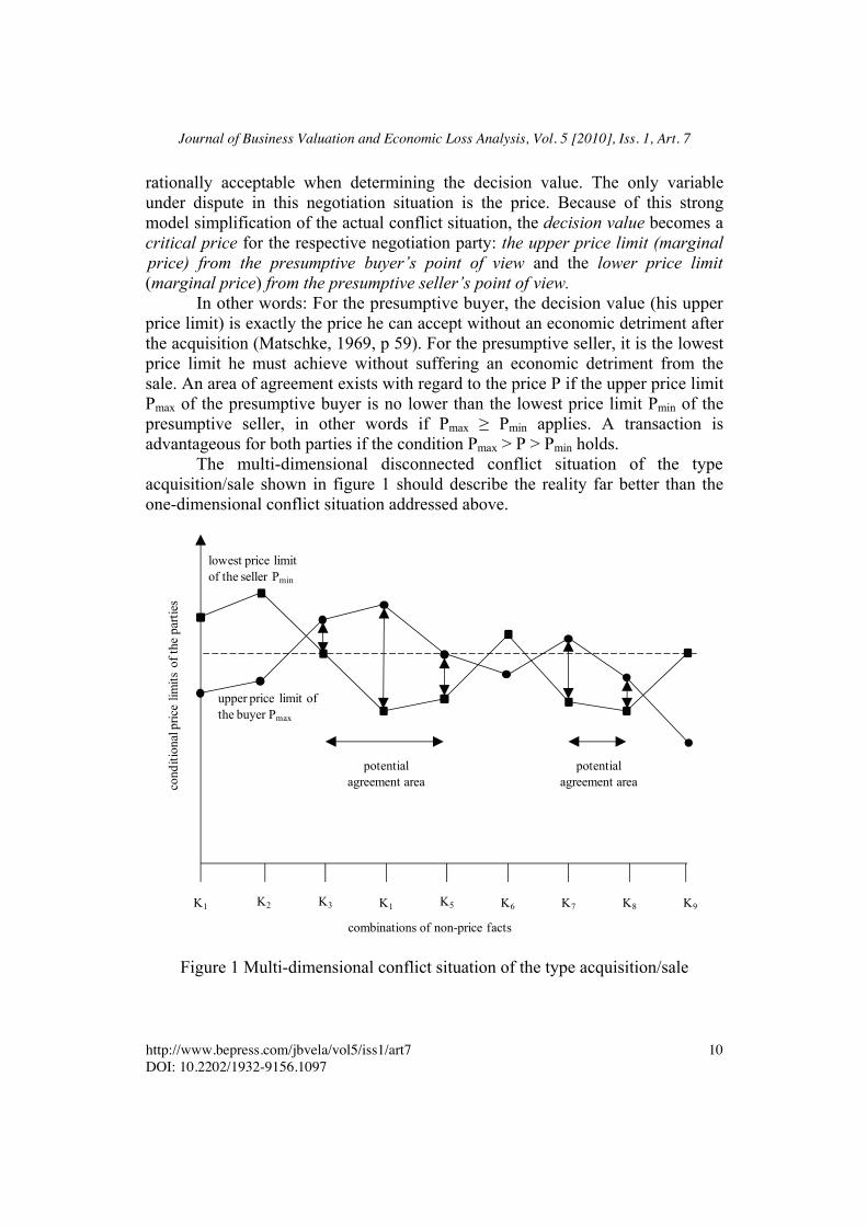
In other words: For the presumptive buyer, the decision value (his upper price limit) is exactly the price he can accept without an economic detriment after the acquisition (Matschke, 1969, p 59). For the presumptive seller, it is the lowest price limit he must achieve without suffering an economic detriment from the sale. An area of agreement exists with regard to the price P if the upper price limit Pmax of the presumptive buyer is no lower than the lowest price limit Pmin of the presumptive seller, in other words if Pmax ≥ Pmin applies. A transaction is advantageous for both parties if the condition Pmax > P > Pmin holds.

The multi-dimensional disconnected conflict situation of the type acquisition/sale shown in figure 1 should describe the reality far better than the one-dimensional conflict situation addressed above.

cond

ition

al p

rice

limits

of t

he p

artie

s

combinations of non-price facts

K1 K2 K3 K6K5K1 K9K8K7

potentialagreement area

potentialagreement area

upper price limit of the buyer Pmax

lowest price limitof the seller Pmin

Figure 1 Multi-dimensional conflict situation of the type acquisition/sale

10



To present this situation graphically, all non-price conflict-resolution-relevant issues regarding different combinations were nominally combined on the abscissa. The price limits of the conflicting parties shall be interpreted as conditional variables. Depending on the non-price components, the buyer might offer more or less and the seller would have to demand more or less.

There are two potential agreement areas in the example, namely the combinations of the non-price facts K3, K4 and K5 on the one hand and of K7 and K8 on the other hand because the upper price limit of the buyer is higher in these cases than the lowest price limit of the seller. Such a multi-dimensional situation requires creativity from both sides to discover the potential areas of agreement.

2. MARGINAL PRICE AS A SPECIAL DECISION VALUE

A) MODEL BASICS

The decision value is calculated in two steps, regardless of the underlying conflict situation.

The first step comprises the determination of the achievable level of utility for the conflicting party without agreement. This step is called determina-tion of the base program.

The second step comprises the establishment of the conflict-resolution-relevant issues that a conflicting party rejects, prefers or judges indifferently because a lower, higher or equal level of utility is achievable from the conflicting party‘s perspective in case of an agreement.

Of special interest for a negotiation is the set of conflict-resolution-relevant issues that results in the same level of utility after an agreement as without an agreement or that results in the lowest possible increase of the level of utility compared to a non-agreement in case of discontinuities. During the nego-tiation, they form the limit of concession willingness, the decision value. The second step is called determination of the valuation program.

Based on this idea, it is possible to develop a general model to determine the decision value from which all other decision value determination methods can be derived. This general model (Matschke, 1975, p 387; Matschke/Brösel, 2007, p 142) does not require the determination of the targets and decision fields of the conflicting parties nor the number and type of conflict-resolution-relevant issues. Its applications are by no means limited to business valuation problems: it is applicable to any number of decision-dependent and interpersonal conflict situations without compulsory character. Because of its general applicability, it is of course extremely complex and very abstract.

Instead, a less complex model shall be presented here, which has the advantage of offering an efficient algorithm to determine the decision value.

11



B) STATE MARGINAL PRICE MODEL – A GENERAL MODEL

The so-called state marginal price model (in German: Zustands-Grenzpreismodell, ZGPM) was developed by Hering (2006).8 This investment model is a theoretical general model based on a one-dimensional, disconnected and non-dominant conflict situation of the type acquisition/sale (Hering/Olbrich/Steinrücke, 2006, p 409; Matschke/Brösel, 2007, p 201).

The decision subject pursues a financial target, for example by maxi-mizing time-structured withdrawals, and acts in an imperfect and incomplete capital market. His planning horizon is finite and extends over T periods, and in each period, investment and financial flows may take place. This model can be adapted to multivalued expectations. For the sake of simplicity, it shall be presented here only under the premise of certainty and only from the purchaser's point of view.

With the state marginal price model, the marginal price of companies can be calculated in two steps based on multi-period, simultaneous planning approaches (Weingartner, 1963; Hax, 1964), using linear optimization methods.

In the first step, the investment and financing program is calculated as the base program. This investment and financing program maximizes the target function under the assumption that the ownership rights are not changed. To determine this base program, an adequate linear optimization approach must be formulated and solved.

The calculation of the base program helps the valuation subject determine the maximum utility level he can achieve without resolution of the conflict situation, i.e., the valuation object is not contained in the base program of the presumptive buyer. The conditions under which maximization is carried out include the loan possibilities, unlimited cash management and available interest-carrying deposits in all periods. Predisposed payments – e.g., from current business activity and existing loan obligations – must be taken into account with a fixed payment balance, which is independent of the objects to be valued, and may be positive, negative, or zero. At any time, the returns from investment and financial objects and the balance of already predisposed payments should be sufficient to allow the distribution to the owner(s) at any time. In other words, the financial balance in the sense of liquidity must exist at all times by maintaining liquidity as condition.

It is then possible to establish the following mathematical approach for the base program from a buyer's point of view:

8 Hering (2006) refers to the general models for marginal price determination of Laux/Franke (1969) as well as of Jaensch (1966) and Matschke (1972, p 153; 1975, p 253).

12



Target function:

ENKBa ! max!

The size of the withdrawal flow expected by the buyer from the base

program ENKBa is maximized under the following restrictions:

Restrictions:

(1) Liquidity constraint (ability to pay at all times): The sum of excess deposits (income) to be realized from investment and financing objects and from current payments may not be smaller than the withdrawals: • at t = 0:

! gKj0 " xKjj=1

J

#deposit surplus

to be realised frominvestment and

financing objects

! "# $#+ w K0 "ENK

Ba

desiredwithdrawal

! "# $#$ bK0

decision!independent

payments

% .

Already at t = 0, an amount of w K 0!ENK

Ba may be withdrawn. bK0 can be interpreted as initially available own investment capital. • at t = 1, 2, …, T:

! gKjt " xKjj=1

J

#deposit surplus

to be realised frominvestment and

financing objects

! "# $#+ w Kt "ENK

Ba

desiredwithdrawal

! "# $#$ bKt

decision!independent

payments

% .

The structure of the desired withdrawals in the future is

w K1 : w K2 : … : w KT!1 : w KT. If e.g., w KT = a +1 / i holds, w KT !ENKBa may

be interpreted as withdrawal amount a !ENKBa

as well as capital amount of

which a continuous equal, permanent withdrawal flow of size ENKBa can be

obtained if it is reinvested with interest. The payments bKt may be interpreted as equity capital increases planned for the future, but also as autonomous future payment obligations, allowing also bKt = 0.

13



(2) Capacity limits (restrictions on the quantity of the investment and financing objects):

The size xKj of the investment and financing objects to be realized may not

violate the respective upper capacity limit (for j =1, 2, …. J):

xKj ! xKj

max .

If capital investment or loan is available without limit, this restriction does not apply.

(3) Non-negativity conditions: The choice variables and the withdrawal flow shall not become negative:

xKj ! 0

ENK ! 0.

The results of this approach are the investments and financings sought to

be realized, which together form the base program of the purchaser. The buyer expects a withdrawal stream with a maximum size of ENK

Ba max from the base program. The withdrawals to be expected at the different points in time t thus are

w Kt !ENKBa max .

During the second step for the here exclusively considered acquisition situation, the valuation object is included in the investment and financing program of the presumptive buyer. The result of this second step is the valuation program, which must include the valuation object in the acquisition situation. To guarantee rational action by the purchaser, the maximum payable purchase price is determined as the decision value on the condition that at least the target function contribution of the base program must be achieved again.

The following approach leads to the determination of the valuation program and the decision value as the upper price limit of the buyer if the future payments from the company are summarized in the payment vector

gUK = (0;gUK1;gUK2; … ;gUKT ) : 9

9 In t = 0, the still to be negotiated price P must be considered as well.

14



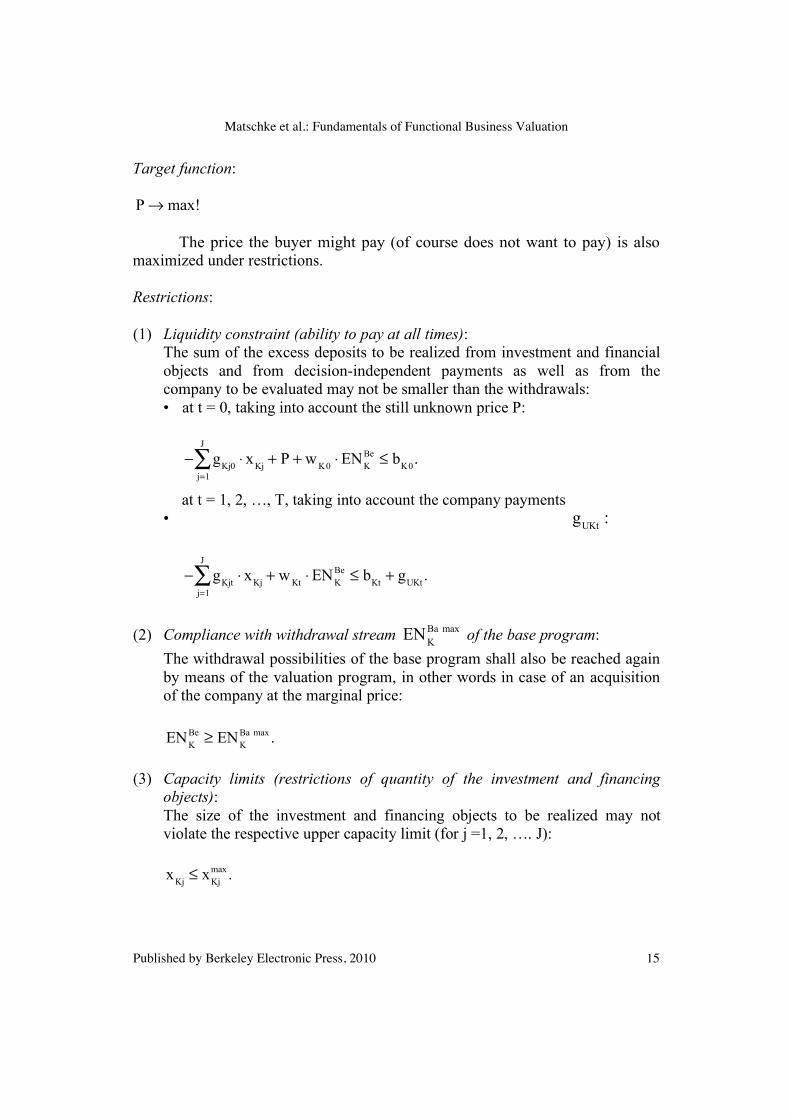
Target function: P ! max!

The price the buyer might pay (of course does not want to pay) is also maximized under restrictions. Restrictions:

(1) Liquidity constraint (ability to pay at all times): The sum of the excess deposits to be realized from investment and financial

objects and from decision-independent payments as well as from the company to be evaluated may not be smaller than the withdrawals: • at t = 0, taking into account the still unknown price P:

! gKj0 " xKj

j=1

J

# + P + w K0 "ENKBe $ bK0.

•

at t = 1, 2, …, T, taking into account the company payments

gUKt :

! gKjt " xKj

j=1

J

# + w Kt "ENKBe $ bKt + gUKt .

(2) Compliance with withdrawal stream ENK

Ba max of the base program: The withdrawal possibilities of the base program shall also be reached again

by means of the valuation program, in other words in case of an acquisition of the company at the marginal price:

ENK

Be ! ENKBa max .

(3) Capacity limits (restrictions of quantity of the investment and financing

objects): The size of the investment and financing objects to be realized may not

violate the respective upper capacity limit (for j =1, 2, …. J):

xKj ! xKj

max .

15



If the capital investment or loan opportunity is unlimited, this restriction does not apply.

(4) Non-negativity conditions: The choice variables should not be negative; in addition, the case of the

buyer being subsidized by the seller (negative purchase price) is excluded:10

xKj ! 0

P ! 0.

The procedure for determining the decision value using the state

marginal price model from the view of a presumptive buyer is now illustrated with an example with a multi-period planning span (T = 4), assuming (quasi-) certain expectations.

The valuation subject already owns a small enterprise KU at the valuation date t = 0, which shall also constitute the decision and acquisition date. The valuation subject manages KU as general manager and receives a permanent deposit surplus from internal financing (IF) in the amount of 30. At t = 0, the valuation subject has the opportunity to make an investment AK. The payment sequence for this investment includes the price payable for it (–100, +30, +40, +50, +55). At t = 0, the valuation subject owns personal assets (EM) from family sources in the amount of 10. It is assumed that the main bank of the general manager in t = 0 makes a total loan ED in the amount of 50 available at an annual interest rate of 8% for investments of the valuation subject with a total term of four periods (years). Additional financial funds are available as operating loans in unlimited amounts at a short-term interest rate of 10% (KAt). Financial invest-ments (GAt) of any amount may be made at the general manager’s main bank at an interest rate of 5% p. a.

The valuation subject aims to achieve a uniform income stream (income maximization) to safeguard its existence. At T = 4, we obtain:

w KT !ENK

Ba = ENKBa +

ENKBa

i" w KT = 1+

1i= 1+

10.05

= 21,

so that the desired time structure reads:

w K0 : w K1 : w K2 : w K3 : w K4 = 1:1:1:1: 21.

10 The withdrawal stream of the base program is not negative. This also applies to the withdrawal stream of the valuation program so that an extra condition is not necessary.

16



This means that in addition to the regular distribution ENKBa , the last distribution

shall contain the cash value or present value of a perpetual annuity based on an interest rate of 5% to guarantee the income ENK

Ba outside the planning period because the estimated interest rate of i = 5% p. a. is taken into account for t > 4 in the example.

At t = 0 the valuation subject may acquire another enterprise U. For this enterprise, the payment stream gUK = (0, 60, 40, 20, 20) was estimated for the planning period. In addition, a permanent annuity in the amount of 20 is expected, starting in t = 5. The valuation subject seeks to determine the maximum payable price Pmax for enterprise U.

In the table below, the data of the example are summarized. In order not to cut the vertical interdependencies between the selected planning period and the periods beyond the planning horizon, the perpetual payment surplus from internal financing and the perpetual annuity expected from the enterprise U starting from time t = 5 were also considered at time t = 4 through the factor 21 (thus including the respective payment due at time t = 4). The payments to be expected after time t > T = 4 are therefore taken into account in the example, using the estimated interest rate i = 5% p. a. (see figure 2).

T AK ED GA0 GA1 GA2 GA3 KA0 KA1 KA2 KA3 EM IF U 0 -100 50 -1 1 10 30 P? 1 30 -4 1.05 -1 -1.1 1 30 60 2 40 -4 1.05 -1 -1.1 1 30 40 3 50 -4 1.05 -1 -1.1 1 30 20 4 55 -54 1.05 -1.1 630 420

Limit 1 1 8 8 8 8 8 8 8 8 1 1 1

Figure 2 Data of the example from the buyer´s point of view

To determine the base program, the given data must be used to formulate a linear optimization approach that can be solved using the simplex algorithm:

17



ENKBa ! max!

100 "AK # 50 "ED +1"GA0 #1"KA0 +1"ENKBa $ 40

#30 "AK + 4 "ED #1.05 "GA0 +1"GA1 +1.1"KA0 #1"KA1 +1"ENKBa $ 30



#55 "AK + 54 "ED #1.05 "GA3 +1.1"KA3 + 21"ENKBa $ 630

AK, ED, GA0, GA1, GA2, GA3, KA0, KA1, KA2, KA3, ENKBa % 0

AK, ED $ 1.

The solution gives the base program whose complete finance schedule is

presented in figure 3:

t = 0 t = 1 t = 2 t = 3 t = 4 Personal assets EM 10 Internal financing IF 30 30 30 30 630 Investment AK -100 30 40 50 55 Loan ED 42.7680 -3.4214 -3.4214 -3.4214 -46.1894 Revolving line KA 49.8496 30.8736 Financial investments GA -43.9610 KA-, GA-paybacks -54.8346 -33.9610 46.1591 Withdrawal EN -32.6176 -32.6176 -32.6176 -32.6176 -32.6176 Payment balance 0 0 0 0 652.3520 Debt level from KA 49.8496 30.8736 Deposits from GA 43.9610 Terminal assets EN/0.05 652.3520

Figure 3 Complete finance schedule of the buyer´s base program

A maximum uniform income stream of the size ENK

Ba max = 32.6176 originates from the base program. At an interest rate of 5% p. a., the assets at the end of the planning period in the amount of 652.3520 are the source of a perpetual annuity of the determined size of ENK

Ba max . The investment AK should be realized. To this end, internal financing IF, personal assets EM and the loan ED of 0.855360 which matures at t = 4 as well as the operating loans KA in t = 0 and t = 1 are used. One-period financial investments GA are made in t = 3. The liquidity constraint is met as the payment balance during the periods t = 1, 2, 3 is 0 while a surplus of 652.3520 results after the deduction of the withdrawal in the amount of ENK

Ba max in t = 4.

18



If the company U is included in the valuation program, at least the size of the uniform income stream of the base program must be reached again. To determine the valuation program, the formulated linear approach must again be solved using the simplex algorithm.

P ! max!

100 "AK # 50 "ED +1"GA0 #1"KA0 +1"ENKBe + P $ 40

#30 "AK + 4 "ED #1.05 "GA0 +1"GA1 +1.1"KA0 #1"KA1 +1"ENKBe $ 90



#55 "AK + 54 "ED #1.05 "GA3 +1.1"KA3 + 21"ENKBe $ 1,050

ENKBe % 32.6176

AK, ED, GA0, GA1, GA2, GA3, KA0, KA1, KA2, KA3, P % 0

AK, ED $ 1.

The complete financing plan of the valuation program is shown below in

figure 4.

t = 0 t = 1 t = 2 t = 3 t = 4 Personal assets EM 10 Internal financing IF 30 30 30 30 630 Company U 60 40 20 420 Investment AK -100 30 40 50 55 Loan ED 50 -4 -4 -4 -54 Revolving line KA 434.0726 394.0975 360.1248 332.7549 Financial investments GA KA-paybacks -477.4799 -433.5073 -396.1373 -366.0304 Withdrawal EN -32.6176 -32.6176 -32.6176 -32.6176 -32.6176 Payment balance 391.4550 0 0 0 652.3520 Debt level from KA 434.0726 394.0975 360.1248 332.7549 Deposits from GA Terminal assets EN/0.05 652.3520

Figure 4 Complete finance schedule of the buyer´s valuation program

The marginal price P max for the company U is 391.4550. In t = 0, the valuation subject invests in company U and, as already in the base program, in object AK. In addition to internal financing IF, personal assets EM, and the loan ED which matures at t = 4, operating loans KA are used in all planning periods.

19



The decision value as the maximum payable price from the buyer's viewpoint can be calculated in tabular form by subtracting the numbers of the valuation program from the base program. This is shown below based on the numerical example to demonstrate which changes must be made to attain the valuation program from the base program. The differences indicate what is called the “comparison object“ in company valuation theory (see figure 5).

The payment stream of the comparison object at t > 0 corresponds to the payment stream of the company under valuation so that there is profit equality between valuation and comparison object. It is the mirror-image of the company under valuation because the buyer must do without the payment stream of the comparison object if the valuation object is acquired. The funds of the comparison object released at t = 0 are the upper price limit for the company under valuation. If the payment streams of the valuation and comparison object are added, payment balances of 0 currency units result for t > 0 since the profitability is the same, whereas a payment balance in the amount of the decision value results in t = 0.

The comparison object in the example are additional operating loans at t = 0, t = 1, t = 2 and t = 3 as well as not executed monetary investments at t = 2 and t = 3. The future payments expected from the additional third party funds as well as from suppressed investments correspond to the surplus deposits of the company so that the payment balance of the comparison object resulting at time t = 0 reflects the amount of the maximum payable price. The buyer's decision value

Pmax of 391.4550 results from this “price“ of the comparison object. Because the payment stream of the comparison object is fixed, its internal interest can be determined. In the example, the internal interest rate of the comparison object from the buyer's point of view is rK = 0.0983642.

The decision-oriented interpretation of the term “comparison object“ has nothing to do with a “comparable“ company as the term is erroneously understood in the literature. Therefore, the issue when determining the decision value is not to find a company comparable to the company under valuation. Rather, all measures to redesign the base program into the valuation program are the comparison object to the company to be evaluated because they constitute the alternative to the acquisition of the company at the decision value.

20



t = 0 t = 1 t = 2 t = 3 t = 4 Valuation program of the buyer Personal assets EM 10 Internal financing IF 30 30 30 30 630 Company U 60 40 20 420 Investment AK -100 30 40 50 55 Loan ED 50 -4 -4 -4 -54 Revolving line KA 434.0726 394.0975 360.1248 332.7549 Financial investments GA KA-paybacks -477.4799 -433.5073 -396.1373 -366.0304 Withdrawal EN -32.6176 -32.6176 -32.6176 -32.6176 -32.6176 Payment balance 391.4550 0 0 0 652.3520 ./. Base program of the buyer Personal assets EM 10 Internal financing IF 30 30 30 30 630 Investment AK -100 30 40 50 55 Loan ED 42.7680 -3.4214 -3.4214 -3.4214 -46.1894 Revolving line KA 49.8496 30.8736 Financial investments GA -43.9610 KA-, GA-paybacks -54.8346 -33.9610 46.1591 Withdrawal EN -32.6176 -32.6176 -32.6176 -32.6176 -32.6176 Payment balance 0 0 0 0 652.3520 = Comparison object (changes between both programs) ∆ Personal assets EM 0 0 0 0 0 ∆ Internal financing IF 0 0 0 0 0 ∆ Investment AK 0 0 0 0 0 ∆ Loan ED 7.2320 -0.5786 -0.5786 -0.5786 -7.8106 ∆ Revolving line KA 384.2230 363.2239 360.1248 332.7549 0 ∆ Financial investments GA 0 0 0 43.9610 0 ∆ KA-paybacks 0 -422.6453 -399.5463 -396.1373 -412.1894 ∆ Withdrawal EN 0 0 0 0 0 = Payment balance of changes (comparison object) 391.4550 -60 -40 -20 -420

Company U 60 40 20 420 Decision value Pmax 391.4550 0 0 0 0

Figure 5 Determination of the buyer´s comparison object

If the expected payments from the company under valuation are discounted at the internal interest rate of this “comparison object“, a future performance value ZEW (in German: Zukunftserfolgswert) equal to the maximum payable price, i.e., the decision value, results (see figure 6).

21



t 0 1 2 3 4 Company U 60 40 20 420

rK 0.098364 (1 + rK)-t 1 0.910445 0.82891 0.754677 0.687091

Cash value/Present value 54.6267 33.1564 15.0935 288.5784 Future performance value ZEW 391.4550

Figure 6 Determination of the decision value from the buyer´s point of view based on the internal interest rate of the comparison object

Thus the decision value can be formally determined by discounting the

future payments of the company to be acquired with the internal interest rate of the comparison object, i.e., as future performance value. However, this does not prove that this method is legitimate. This issue shall be discussed below.

C) FUTURE PERFORMANCE VALUE METHOD – A PARTIAL MODEL

The future performance value method is a partial model which only takes into account the valuation object and not the entity of all possible actions of the decision model. Compared to the total model “state marginal price model”, a company valuation loses a substantial amount of complexity if the partial model “future performance value method” (in German: Zukunftserfolgswertmethode) is used.

Depending on the structure of the expected payments, the determination of the future performance value ZEW can be based on different valuation formu-las of which the most important variations will be discussed below:

1. for a finite planning horizon of T periods with differing or constant future financial performances11 ZE (in German: Zukunftserfolg) and flat12 interest structure (same interest rate i during all periods 1 to T):

ZEW =

ZEt

(1+ i)tt=1

T

! or – when ZEt = ZE = const. – ZEW = ZE "(1+ i)T #1i " (1+1)T

.

11 The term “future performance” means future surplus deposits expected by the decision subject from the business under valuation. “Future performance value” is the sum of the present values of the future performance. The present values are determined by discounting. 12 In case of a “flat” interest structure the interest rate is constant, independent of the investment period t.

22



2. for a finite planning horizon of T periods with different future financial performances ZE and non-flat13 interest structure (differing interest rates during periods 1 to T):

ZEW =ZEt

(1+ i! )!=1

t

"t=1

T

# .

3. for an infinite planning horizon with constant future financial performances

ZE and flat interest structure:

ZEW = lim

T!"ZE #

(1+ i)T $1i # (1+1)T =

ZEi

.

4. for an infinite planning horizon with different future financial performances

during the first T periods and subsequent constant future financial performances and flat interest structure:

ZEW =

ZEt

(1+ i)tt=1

T

! +ZET+1

i"

1(1+ i)T .

5. for a finite planning horizon with different future financial performances

during the first T periods and subsequent future financial performances increasing at rate w for n periods and flat interest structure (with w ! i):

ZEW =ZEt

(1+ i)tt=1

T

! + ZET+1 "1

(1+ i)T "1

i # w" 1#

1+ w1+ i

$%&

'()

n+1$

%&&

'

())

.

6. for an infinite planning horizon with different future financial performances

during the first T periods and subsequent future financial performances increasing infinitely at rate w and flat interest structure (with w < i):

13 In case of a “non-flat” interest structure the interest rate differs depending on period t: in case of a “normal” interest structure it is increasing in t, in case of an “inverse” interest structure it is decreasing in t.

23



ZEW =

ZEt

(1+ i)tt=1

T

! + ZET+1 "1

(1+ i)T "1

i # w.

These formulas only explain the actuarial basis of the future performance

value method as a current value method, but do not explain whether the future performance value constitutes a decision value in the sense of a marginal price.

The issue is: Why is this procedure legitimate? Can the current value calculation prove to be a sensible process to determine the decision value as the future performance value from the viewpoint of a buyer or seller in case of a purely actuarial target, as generally assumed without further inspection? How can the necessary calculation interest rates i for the decision value determination be found? Are the interests of the valuation subjects preserved if the future performance value method is applied and if yes, why?

The use of this method to determine the decision value is only legitimate if the future performance value formula can be theoretically explained. Perhaps its applicability limits can be determined, so that the assumptions that have to be made in case of its application are indicated. Also, the following questions could then be answered: What results if these assumptions are not strictly fulfilled? Is the future performance value formula still helpful?

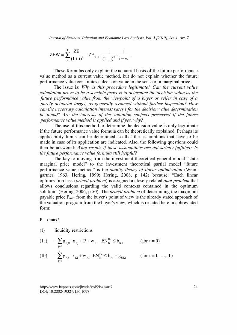
The key to moving from the investment theoretical general model “state marginal price model” to the investment theoretical partial model “future performance value method” is the duality theory of linear optimization (Wein-gartner, 1963; Hering, 1999; Hering, 2008, p 142) because: “Each linear optimization task (primal problem) is assigned a closely related dual problem that allows conclusions regarding the valid contexts contained in the optimum solution” (Hering, 2006, p 50). The primal problem of determining the maximum payable price Pmax from the buyer's point of view is the already stated approach of the valuation program from the buyer's view, which is restated here in abbreviated form:

P ! max!

(1) liquidity restrictions

(1a) " gKj0 # xKjj=1

J

$ + P + w K0 #ENKBe % bK0 (for t = 0)

(1b) " gKjt # xKjj=1

J

$ + w Kt #ENKBe % bKt + gUKt (for t = 1, …, T)

24



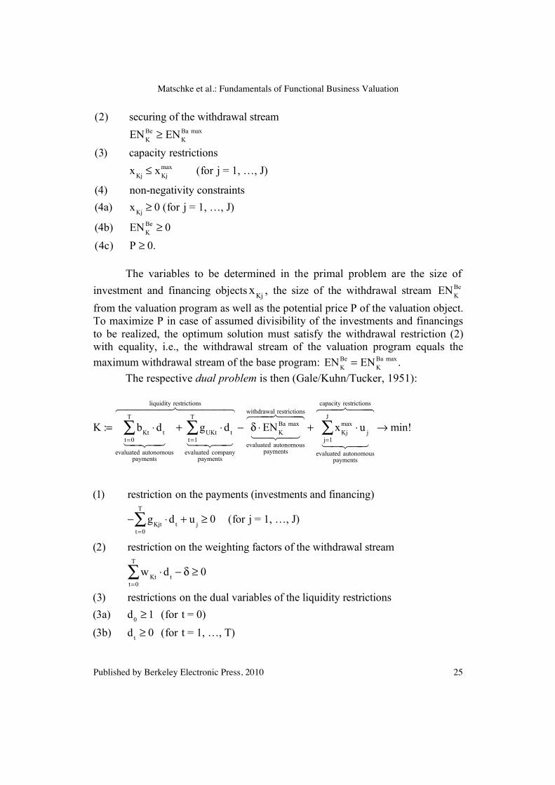
(2) securing of the withdrawal stream

ENKBe & ENK

Ba max

(3) capacity restrictions

xKj % xKjmax (for j = 1, …, J)

(4) non-negativity constraints(4a) xKj & 0 (for j = 1, …, J)

(4b) ENKBe & 0

(4c) P & 0.

The variables to be determined in the primal problem are the size of

investment and financing objects xKj , the size of the withdrawal stream ENKBe

from the valuation program as well as the potential price P of the valuation object. To maximize P in case of assumed divisibility of the investments and financings to be realized, the optimum solution must satisfy the withdrawal restriction (2) with equality, i.e., the withdrawal stream of the valuation program equals the maximum withdrawal stream of the base program: ENK

Be = ENKBa max .

The respective dual problem is then (Gale/Kuhn/Tucker, 1951):

K := bKt !dtt=0

T

"evaluated autonomous

payments

! "# $#+ gUKt !dt

t=1

T

"evaluated company

payments

! "# $#

liquidity restrictions% &#### '####

# $ !ENKBa max

evaluated autonomouspayments

! "# $#

withdrawal restrictions% &## '##+ xKj

max !u jj=1

J

"evaluated autonomous

payments

! "# $#

capacity restrictions% &## '##

% min!

(1) restriction on the payments (investments and financing)

# gKjt !dtt=0

T

" + u j & 0 (for j = 1, …, J)

(2) restriction on the weighting factors of the withdrawal stream

w Kt !dtt=0

T

" # $ & 0

(3) restrictions on the dual variables of the liquidity restrictions(3a) d0 & 1 (for t = 0)

(3b) dt & 0 (for t = 1, …, T)

25



(4a) restrictions on the dual variables of the capacity restrictionsu j & 0 (for j = 1, …, J)

(4b) restrictions on the dual variables for the securing of the withdrawal stream$ & 0.

The autonomous payments bKt correspond to the right -hand sides of the

payment restrictions of the valuation program without the payments from the company under valuation, i.e., the right-hand sides of the payment restrictions of the base program. The evaluated right-hand sides of the restrictions of the primal problem are in the target function of the dual program. The variables of the dual problem to be determined are the dual variables dt (for the liquidity constraint in t = 0, …, T), uj (for the capacity restrictions with j = 1, …, J) and δ (for the restriction of securing the withdrawal stream). The dual variables shall be established in the optimum of the dual problem so that the sum of the evaluated right-hand sides of the restrictions, i.e., the opportunity costs K of these restrictions, becomes as small as possible. The optimum solution of the dual problem is then Kmin.

From the conditions ENKBe = ENK

Ba max and ENKBe ≥ 0 in the primal

problem and from ENKBa max

> 0 as the optimal solution of the base program, it

follows that the withdrawal restriction (2) at the optimum of the dual problem must equal the following:

w Kt !dtt=0

T

" # $ % 0

and

$ = w Kt !dtt=0

T

" .

It holds that the maximum of the primal problem (with solution: Pmax) equals the minimum of the dual problem (with solution: Kmin). Because of this relationship, the definition equation of K may be used to calculate Pmax. If the solution for δ is considered, the following equation for the decision value Pmax results:

26



Pmax = bKt !dt

t=0

T

" + gUKt !dtt=1

T

" + xKjmax !u j

j=1

J

" # ENKBa max ! w Kt !dt

t=0

T

" .

In the optimal solution of the primal problem, P = Pmax > 0 holds, thus

the liquidity constraint (1a) of the primal problem is slack. It follows from the theorem of complementary slackness that the restriction (3a) must be binding so that d0 = 1 holds. The dual variable d0 = 1 means that today's payments are included in the calculation of Pmax without modification. For the other dual values

dt for t = 1, …, T the relation dt / d0 =:!KtBe holds. !Kt

Be are to be interpreted as discount factors for the valuation program, which may be derived from the endogenous period marginal interest rates iKt

Be of the valuation program of the buyer (Rollberg, 2001, p 178; Hering, 2008, p 182):

!KtBe =

1

(1+ iK"Be )

"=1

t

#.

This means: 1 currency unit of the time period t > 0 is then worth !Kt

Be currency units at t = 0 so that future payments are included in the calculation of Pmax with their cash value, or in other words are converted.

For investment and financing objects j contained in the valuation program, restriction (1) of the dual problem is satisfied at its lower limit:

! gKjt "dt

t=0

T

# + u j = 0 $ u j = gKjt "dtt=0

T

#

and a non-negative capital value (as net-present value)

CKj

Be ! 0 at t = 0 results.

Since CKj

Be constitutes a current monetary value, it follows from the theory of

marginal cost pricing that CKj

Be !d0 = u j holds and consequently, u j and CKj

Be are identical because d0 = 1.

In case of disadvantageous investment and financing objects, the restriction (1) of the dual problem is slack. It follows that the restriction (4a) of the dual problem must be binding, hence the dual variable

u j is 0 for disadvan-

tageous investment and financing objects with negative capital value.

27



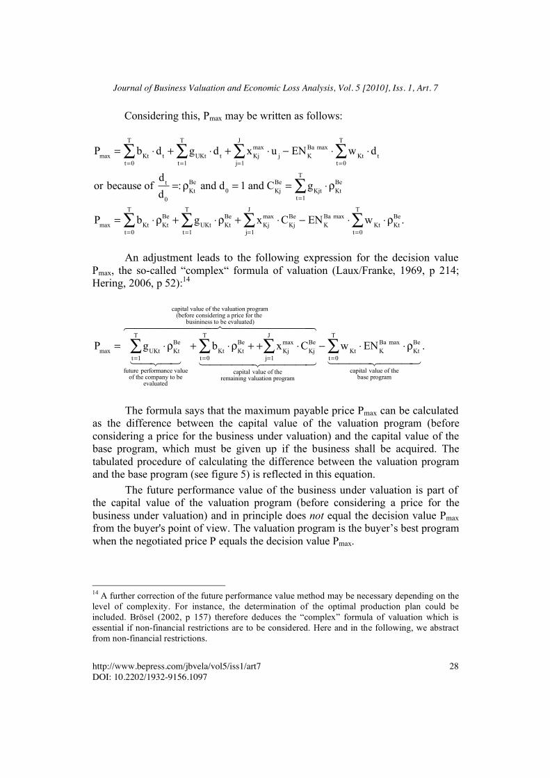
Considering this, Pmax may be written as follows:

Pmax = bKt !dtt=0

T

" + gUKt !dtt=1

T

" + xKjmax !u j

j=1

J

" # ENKBa max ! w Kt !dt

t=0

T

"

or because of dt

d0

=:$KtBe and d0 = 1 and CKj

Be = gKjt ! $KtBe

t=1

T

"

Pmax = bKt ! $KtBe

t=0

T

" + gUKt ! $KtBe

t=1

T

" + xKjmax !CKj

Be

j=1

J

" # ENKBa max ! w Kt ! $Kt

Be

t=0

T

" .

An adjustment leads to the following expression for the decision value

Pmax, the so-called “complex“ formula of valuation (Laux/Franke, 1969, p 214; Hering, 2006, p 52):14

Pmax = gUKt ! "KtBe

t=1

T

#future performance value

of the company to beevaluated

! "# $#+ bKt ! "Kt

Be

t=0

T

# + + xKjmax !CKj

Be

j=1

J

#capital value of the

remaining valuation program

! "#### $####

capital value of the valuation program(before considering a price for the

busininess to be evaluated)% &######## '########

$ w Kt !ENKBa max ! "Kt

Be

t=0

T


base program

! "### $###.

14 A further correction of the future performance value method may be necessary depending on the level of complexity. For instance, the determination of the optimal production plan could be included. Brösel (2002, p 157) therefore deduces the “complex” formula of valuation which is essential if non-financial restrictions are to be considered. Here and in the following, we abstract from non-financial restrictions.

The formula says that the maximum payable price Pmax can be calculated as the difference between the capital value of the valuation program (before considering a price for the business under valuation) and the capital value of the base program, which must be given up if the business shall be acquired. The tabulated procedure of calculating the difference between the valuation program and the base program (see figure 5) is reflected in this equation.

The future performance value of the business under valuation is part of the capital value of the valuation program (before considering a price for the business under valuation) and in principle does not equal the decision value Pmax from the buyer's point of view. The valuation program is the buyer’s best program when the negotiated price P equals the decision value Pmax.

28



Rearrangements lead to the following formula for the decision value Pmax from the buyer's point of view:

Pmax = gUKt

payments ofthe valuation

object!! "Kt

Be

discountfactor!

t=1

T

#future performance value

of the company to beevaluated

" #$$ %$$+ bKt ! "Kt

Be

t=0

T

# + xKjmax !CKj

Be

CKj >0#

sum of thepositive capital

values& '$$ ($$

capital value of the valuation program(without the valuation object)

" #$$$$ %$$$$

$ w Kt !ENKBa max ! "Kt

Be

t=0

T


base program

" #$$$ %$$$

change of the capital value as a result of transforming the base programto the valuation program % 0

" #$$$$$$$$$ %$$$$$$$$$

.

According to this, the maximum payable price Pmax as the buyer’s

decision value results from the future performance value of the business ZEW, taking into account the capital value difference by transforming the base program into the valuation program of the buyer :

Pmax = ZEWUK (!Kt

Be ) + "KWKBe#Ba with "KWK

Be#Ba $ 0, so that

ZEWUK (!Kt

Be ) = Pmax # "KWKBe#Ba

or

ZEWUK (!Kt

Be ) % Pmax .

The future performance value based on endogenous marginal interest

rates of the valuation program thus constitutes a lower limit for the buyer’s decision value.

The question is now whether it is also possible to determine an upper limit for the buyer's decision value. This is indeed possible. The starting point is the dual problem for the determination of the buyer's base program (Hering, 2006, p 55). It can be shown that the capital value difference !KWK

Be"Ba is actually not negative, as assumed in the calculation equation. The upper limit for the buyer's decision value corresponds to the future performance value ZEWU

K (!KtBa ) calculated with the

discount factors resulting from the base program. The future performance value can be calculated using the so-called formula of “simplified”15 valuation (using the endogenous marginal interest rates of the base program):16

15 This means that the calculation is only based on the payments of the company under valuation without consideration of the transformation from the base program into the valuation program. 16 That the future performance value on the basis of the endogenous marginal interest rates of the base program has to be the upper limit for the decision value Pmax of the buyer follows from a

29



be calculated using the so-called formula of “simplified”15 valuation (using the endogenous marginal interest rates of the base program):16

Pmax ! gUkt "1

(1+ iK#Ba )

#=1

t

$

discount factor! "# $#

t=1

T

%

future performance valueof the valuation object

based on the endogenousinterest rates of the

base program

% &### '###

= ZEWUK (&Kt

Ba )

under the constraint

ZEWUK (!Kt

Ba ) " Pmax .

The buyer's decision value Pmax must consequently lie between the following limits (Hering, 2006, p 57):17

plausible consideration: If Pmax exceeded the future performance value, paying Pmax would be unprofitable because the capital value would be negative. 17 Concerning this interval, see Brösel (2002, p 166), in case that non-financial restrictions have to be considered.

ZEWUK (!Kt

Be ) " Pmax " ZEWUK (!Kt

Ba )

or

gUkt #1

(1+ iK$Be )

$=1

t

%


t=1

T

&


based on the endogenousinterest rates of the valuation program

% &### '###

" Pmax " gUkt #1

(1+ iK$Ba )

$=1

t

%


t=1

T

&


based on the endogenousinterest rates of the

base program

% &### '###

.

The lower limit is the future performance value based on the endogenous marginal interest rates of the valuation program, the upper limit is the future

30



interest rates differ between the base and valuation program, the valuation problem can only be solved using a general model (Laux/Franke, 1969, p 206; Moxter, 1983, p 143). Based on the partial model, at least the limits for the decision value can be derived.

In an imperfect and incomplete capital market and without knowledge of the solution of the total model, the future performance value procedure is a procedure that narrows down the area in which the buyer's decision value Pmax will lie. For this purpose, it is necessary to estimate endogenous marginal interest rates of the base program and the valuation program as precisely as possible. Even in case of certainty, there is vagueness in the application of the future performance value method as a partial model regarding the determination of the relevant decision value. This vagueness results from the imperfection of the capital market and the resulting differences between the endogenous marginal interest rates of base and valuation program.18

In the numerical example of the decision value determination from the buyer's point of view, the state marginal price model was used to compute a

18 If the endogenous marginal interest rates of both programs are equal, transformations between the base program and the valuation program are realized with a capital value of zero i.e.

!KWKBe"Ba = 0. Only marginal objects are replaced or additionally included. In such a situation,

the “simplified“ valuation formula of the future performance value can be used as a method to calculate the exact decision value as maximum payable price from the buyer's point of view. The “simplified” valuation formula of the future performance value method to calculate the buyer's decision value is always applicable in case of a perfect capital market because marginal transactions are always carried out at the current market interest rate i. Based on this, the following holds if we also assume that the interest rate is constant through time: !Kt

Be = !KtBa = (1+ i)"1.

maximum payable price of 391.455 currency units. From the dual problem of the base program (see figure 4), it follows that the endogenous marginal interest rates are 10% in the first and second period, 6.39% in the third and 5% in the fourth period.19

19 As a result of the resolution of the dual problem of the base program, the following (rounded) dual prices are calculated for the liquidity restriction: d0 = 0.05249704, d1 = 0.04772458, d2 = 0.04338599, d3 = 0.0407805, d4 = 0.03883866. The respective discount factors of the period t are

!t = dt/d0. The endogenous marginal interest rates it of the period t are derived from the relation

it = !t"1 / !t "1.

performance value based on the endogenous marginal interest rates of the base program (computed with the formula of “simplified” valuation). If the marginal

31



Time t 0 1 2 3 4 Company U 60 40 20 420 Endogenous marginal interest rates of the base program

iKtBa 0.1 0.1 0.0639 0.05

Discounting factor !KtBa 0.9090909 0.8264463 0.7768082 0.7398174

Present value/Cash value 54.5455 33.0579 15.5362 310.7233

ZEWUK (!Kt

Be ) 413.8628 Endogenous marginal interest rates of the valuation program

iKtBe 0.1 0.1 0.1 0.1

Discounting factor !KtBe 0.9090909 0.8264463 0.7513148 0.6830135

Present value/Cash value 54.5455 33.0579 15.0263 286.8657

ZEWUK (!Kt

Be ) 389.4953

Figure 7 Upper and lower limit of the decision value Pmax

Figure 8 contains the synopsis of the data for the “complex” calculation formula. Because of the assumed knowledge of the endogenous marginal interest rates, it directly provides the buyer’s exact decision value Pmax.20

20 To make clear that the borrowing of operating loans KA are the marginal transactions, their summarized payments are listed and their capital value is calculated.

In the valuation program, the marginal transactions (see figure 5) are exclusively the borrowing of operating funds KA at 10%.

In figure 7, the data of the example are consolidated and the upper limit and lower limit of the maximum payable amount from the buyer's point of view are calculated. As expected, ZEWU

K ( !KtBe ) " Pmax " ZEWU

K ( !KtBa ) holds or in

numerical values: 389.4953 < Pmax = 391.4550 < 413.8628.

32



Time 0 1 2 3 4 Right-hand side of the payment restrictions of the valuation program (without payments of the company to be evaluated) Right-hand side bKt 40 30 30 30 630 Discounting factors !Kt

Be 1 0.9090909 0.8264463 0.7513148 0.6830135 Present value bKt ! "Kt

Be 40 27.2727 24.7934 22.5394 430.2985 Present value sum bKt ! "Kt

Be# 544.9040

Capital value Investment AK -100 30 40 50 55 Discounting factors !Kt

Be 1 0.9090909 0.8264463 0.7513148 0.6830135 Present value investment AK -100 27.2727 33.0579 37.5657 37.5657 Capital value investment AK 35.4621

Total loan ED 50 -4 -4 -4 -54 Discounting factors !Kt

Be 1 0.9090909 0.8264463 0.7513148 0.6830135 Present value total loan ED 50 -3.6364 -3.3058 -3.0053 -36.8827 Capital value total loan ED 3.1699

Operating loan KA 434.1446 -83.3867 -73.3867 -63.3867 -366.1202 Discounting factors !Kt

Be 1 0.9090909 0.8264463 0.7513148 0.6830135 Present value operating loan 434.1446 -75.8061 -60.6502 -47.6234 -250.0650 Capital value operating loan 0

Withdrawals w Kt !ENKBa max 32.6176 32.6176 32.6176 32.6176 684.9696

Discounting factors !KtBe 1 0.9090909 0.8264463 0.7513148 0.6830135

Present value withdrawals 32.6176 29.6524 26.9567 24.5061 467.8435 Capital value base program 581.5762

ZEWUK (!Kt

Be ) 389.4953 + Present value sum

bKt ! "KtBe# 544.9040

+ Capital value AK 35.4621 583.5360 + Capital value ED 3.1699

Cash value sum of + the remaining valuation program

– Capital value base program -581.5762 Sum = Pmax 391.4550

Figure 8 Components of the “complex” calculation formula for the buyer

33



DISTINGUISHING BETWEEN FUNCTIONAL AND MARKET VALUE-ORIENTED BUSINESS VALUATION

The main differences between functional and market value-oriented business valuation shall now be discussed on the basis of the prior explanations.

Functional business valuation is strongly individualistic in its main functions, i.e., it is directed toward the concrete goals, plans, expectations and action possibilities of the valuation subjects in imperfect and incomplete markets. It is also conflict-oriented, i.e., directed at a possible interpersonal conflict in connection with ownership changes between only a few decision subjects and with several conflict-relevant issues. Functional business valuation considers real existing conditions that are illustrated in a model-theoretically simplified way, but may be examined intersubjectively.

In contrast, the today widespread so-called market value oriented valuation establishes an idealized model world based on the neo-classical finance theory.21 It is geared towards the anonymous, exchange-organized ideal and complete capital market and towards the capital providers acting in it, i.e., it is superindividually oriented. The starting point of this approach is not a specific task because the purpose-dependency of the value is not recognized. In addition, it has another serious deficiency: In contrast to the older objective theory, this younger objective valuation concept denies the difference between value and price and is thus incredibly unrealistic.

Regarding the market assumed by the representatives of the market-oriented valuation, it is assumed that homogeneous (equal) goods are traded at the same time (i.e., on the same market) at the same price. The degree of knowledge of all market participants is the same: the conclusions from the available information coincide. The individual market participant has no market power in this market. The price is given. Value and price must coincide under these ideal market conditions by assumption.22

The so-called market-value oriented valuation has thus completely ignored and forgotten the simplest references to the conditions of real capital markets. 21 For the neo-classical valuation theory and for the classical Anglo-American valuation theory, see e.g. Dean (1951), Hirshleifer (1958), Weingartner (1963). The neo-classical valuation theory rejects the classical theory. 22 These assumptions are an ideal and complete market as well as perfect competition. An ideal market means all market participants are aware of the returns (payment flows) of all traded securities and the returns are equal for all market participants depending on their amount and their temporal structure. A complete market means all possible states can be reproduced by linearly combining traded securities (payment flows), so that any payment flows can be reproduced by traded securities. Perfect competition says that no market participant has market power and is able to influence the prices of the traded securities (Debreu, 1959; Arrow, 1964).

34



The representatives of the market-value-oriented valuation do not ask what the purpose of the valuation is, but concentrate on the valuation process by which one can allegedly determine the “market value“. But even an economics freshman knows that the market value (market price) is derived as an exchange value determined by supply and demand and that gains of trade arise precisely because the average buyer valuation is higher and the average seller valuation is lower than this market price.

The market-value-oriented valuation was deliberately not discussed in this article. This concept that has covered business valuation theory like mildew should be sufficiently familiar, in particular since the so-called discounted cash flow method that allegedly determines the market value constitutes a consulting product offered worldwide. The “theoretical“ discussion of these methods revolves around the futile question of how different DCF methods can be made to lead to the same valuation result – a problem that already existed for the representatives of the older objective concept. At that time as well as today, different valuation results are considered annoying. They may undermine the belief in the validity of the presented “market value” and consequently the authority of the appraisers as secular “cast of priests” who know the secrets of the “market value”, which may thus negatively affect their financial interests.

No single DCF method (WACC-approach, Entity-approach, Equity-approach, APV-approach) has a decision-theoretical foundation (Hering/Olbrich/ Steinrücke, 2006, p 411). However, the DCF methods offer a fertile ground for argumentation values due to their numerous inherent possibilities of manipulation. From the viewpoint of the functional business valuation theory, these methods can be used to bolster arguments brought forward by a conflicting party during a negotiation under two conditions:

1. the value so determined may not violate the decision value of the arguing person;

2. the conflicting party using it as an argumentation aid must be convinced that it may impress the other negotiating party and lead to a result more favorable for the arguing party.

Any conflicting party should however know the exact limits of the applicability of the used DCF methods and should never forget that these methods cannot determine the limit of the concession willingness, i.e., the decision value.

35



CONCLUSION

This article gives an introduction to the concept of functional business valuation. Functional business valuation differs from other business valuation methods in that it recognizes that there does not exist just one value for an enterprise, but that there coexist different values of an enterprise depending on the person for whom the valuation is conducted and the purpose of the valuation. Functional business valuation also takes into account that the typical enterprise is not traded publicly, so that any valuation based on the assumption of perfect capital markets and perfect competition is out of place. Moreover, even if a company is publicly traded, the value for a whole business cannot be appropriately determined by just multiplying the market value of a single share with the total number of shares.

After having introduced the reader to the basic ideas and terminology of functional business valuation, we use detailed numerical examples to explain how a one-dimensional decision value for an undominated purchase/sale situation can be determined. In the example, we first work with a more complex framework, the so-called “state marginal price model”, and then show under which conditions a simplified procedure, the so-called “future performance value method”, can be employed. We also compare the popular market-based valuation methods, such as the discounted cash flow method, and the functional business valuation method.

REFERENCES

Arrow, K.J. (1964) The Role of Securities in the Optimal Allocation of Risk-bearing. Review of Economic Studies, Vol. 31, pp. 91–96.

Brösel, G. (2002) Medienrechtsbewertung. Wiesbaden, DUV. Brösel, G. (2006) Eine Systematisierung der Nebenfunktionen der funktionalen

Unternehmensbewertungstheorie. Betriebswirtschaftliche Forschung und Praxis, Vol. 58, pp. 128–143.

Dean, J. (1951) Capital Budgeting. New York, Columbia University Press. Debreu, G. (1959) Theory of Value. New Haven and London, Wiley. Gale, D., Kuhn, H.W., Tucker, A.W. (1951) Linear Programming and the

Theory of Games. Koopmans, T.C. (ed.), Activity Analysis of Production and Allocation. New York, London, pp. 317–329.

36



Goetzke, W., Sieben, G. (eds.) (1977) Moderne Unternehmungsbewertung und Grundsätze ihrer ordnungsmäßigen Durchführung. Köln, GEBERA.

Gorny, C. (2002) Unternehmensbewertung in Verhandlungsprozessen. Wies-

baden, DUV. Gossen, H.H. (1854) Entwickelung der Gesetze des menschlichen Verkehrs, und

der daraus fließenden Regeln für menschliches Handeln. Braunschweig, Prager.

Hax, H. (1964) Investitions- und Finanzplanung mit Hilfe der linearen Pro-

grammierung. Schmalenbachs Zeitschrift für betriebswirtschaftliche For-schung. Vol. 16, pp. 430–446.

Hering, T. (1999) Finanzwirtschaftliche Unternehmensbewertung. Wiesbaden,

DUV. Hering, T. (2006) Unternehmensbewertung. 2nd edition, Munich and Vienna,

Oldenbourg. Hering, T. (2008) Investitionstheorie. 3rd edition, Munich, Oldenbourg. Hering, T., Olbrich, M., Steinrücke, M. (2006) Valuation of start-up internet

companies. International Journal of Technology Management, Vol. 33, pp. 406–419.

Hirshleifer, J. (1958) On the Theory of Optimal Investment Decision. Journal of

Political Economy, Vol. 66, pp. 329–352. Institut der deutschen Wirtschaft (ed.) (2009) Deutschland in Zahlen 2009.

Cologne, Deutscher Instituts-Verlag GmbH (DIV). Jaensch, G. (1966) Ein einfaches Modell der Unternehmungsbewertung ohne

Kapitalisierungszinsfuß. Schmalenbachs Zeitschrift für betriebswirtschaft-liche Forschung, Vol. 18, pp. 660–679.

Jevons, W.S. (1871) The Theory of Political Economy, London and New York,

Macmillan. Klingelhöfer, H.E. (2006) Finanzwirtschaftliche Bewertung von Umweltschutz-

investitionen. Wiesbaden, DUV.

37



Laux, H., Franke, G. (1969) Zum Problem der Bewertung von Unternehmungen und anderen Investitionsgütern. Unternehmensforschung, Vol. 13, pp. 205–223.

Mandl, G., Rabel, K. (1997) Unternehmensbewertung. Vienna and Frankfurt/

Main. Matschke, M.J. (1969) Der Kompromiß als betriebswirtschaftliches Problem

bei der Preisfestsetzung eines Gutachters im Rahmen der Unternehmungs-bewertung. Schmalenbachs Zeitschrift für betriebswirtschaftliche For-schung, Vol. 21, pp. 57–77.

Matschke, M.J. (1971) Der Arbitrium- oder Schiedsspruchwert der Unterneh-

mung – Zur Vermittlerfunktion eines unparteiischen Gutachters bei der Un-ternehmungsbewertung. Betriebswirtschaftliche Forschung und Praxis, Vol. 23, pp. 508–520.

Matschke, M.J. (1972) Der Gesamtwert der Unternehmung als Entscheidungs-

wert. Betriebswirtschaftliche Forschung und Praxis, Vol. 24, pp. 146– 161. Matschke, M.J. (1975) Der Entscheidungswert der Unternehmung. Wiesbaden,

Gabler. Matschke, M.J. (1976) Der Argumentationswert der Unternehmung – Unter-

nehmungsbewertung als Instrument der Beeinflussung in der Verhandlung. Betriebswirtschaftliche Forschung und Praxis, Vol. 28, pp. 517–524.

Matschke, M.J. (1979) Funktionale Unternehmungsbewertung, Vol. II, Der Ar-

bitriumwert der Unternehmung. Wiesbaden, Gabler. Matschke, M.J. (1981) Unternehmungsbewertung in dominierten Konfliktsitua-

tionen am Beispiel der Bestimmung der angemessenen Barabfindung für den ausgeschlossenen oder ausscheidungsberechtigten Minderheits-Kapitalgesell-schafter. Betriebswirtschaftliche Forschung und Praxis, Vol. 33, pp. 115–129.

Matschke, M.J., Brösel, G. (2007) Unternehmensbewertung. 3rd edition, Wies-

baden, Gabler. Menger, C. (1871) Grundsätze der Volkswirthschaftslehre. Vienna, Braumüller.

38



Moxter, A. (1983) Grundsätze ordnungsmäßiger Unternehmensbewertung. 2nd edition, Wiesbaden, Gabler.

Münstermann, H. (1966) Wert und Bewertung der Unternehmung. Wiesbaden,

Gabler. Olbrich, M. (1999) Unternehmungskultur und Unternehmungswert. Wiesbaden,

DUV. Olbrich, M., Brösel, G., Haßlinger, M. (2009) The Valuation of Airport Slots.

Journal of Air Law and Commerce, Vol. 74, pp. 897–917. Rollberg, R. (2001) Integrierte Unternehmensplanung. Wiesbaden, DUV. Schmalenbach, E. (1937) Finanzierungen. 6th edition, Leipzig, Gloeckner. Schneider, D. (2001) Betriebswirtschaftslehre, Vol. 4: Geschichte und Metho-

den. Munich and Vienna, Oldenbourg. Sieben, G. (1976) Der Entscheidungswert in der Funktionenlehre der Unterneh-

mensbewertung. Betriebswirtschaftliche Forschung und Praxis, Vol. 28, pp. 491–504.

Sieben, G., Löcherbach, G., Matschke, M.J. (1974) Bewertungstheorie. Grochla,

E., Wittmann, W. (eds.), Handwörterbuch der Betriebswirtschaft, Vol. 1, 4th edition, Stuttgart, Schäffer-Poeschel, col. 839–851.

Tillmann, A. (1998) Unternehmensbewertung und Grundstückskontaminatio-

nen. Wiesbaden, DUV. Walras, L. (1874) Éléments d’économie politique pure ou théorie de la richesse

sociale. Lausanne et al., Corbaz. Weingartner, H.M. (1963) Mathematical Programming and the Analysis of Ca-

pital Budgeting Problems. Englewood Cliffs (New Jersey), Prentice Hall.

39



Documents

Journal of Business Valuation and Economic Loss Analysis · Volume 5, Issue 1 2010 Article 7 Journal of Business Valuation and Economic Loss Analysis Fundamentals of Functional Business