Journal of Applied Geophysics 79 (2012) 90–99

Contents lists available at SciVerse ScienceDirect

Journal of Applied Geophysics

j ourna l homepage: www.e lsev ie r .com/ locate / jappgeo

Curvelet-based POCS interpolation of nonuniformly sampled seismic records

Pengliang Yang ⁎, Jinghuai Gao, Wenchao ChenXi'an Jiaotong University, Xi'an, 710049, China

⁎ Corresponding author. Tel.: +86 29 82668771; fax:E-mail addresses: ypl_2100@yahoo.com.cn (P. Yang)

(J. Gao), wencchen@mail.xjtu.edu.cn (W. Chen).

0926-9851/$ – see front matter © 2011 Elsevier B.V. Alldoi:10.1016/j.jappgeo.2011.12.004

a b s t r a c t

a r t i c l e i n f o

Article history:Received 28 October 2011Accepted 13 December 2011Available online 23 December 2011

Keywords:Curvelet transformSeismic data interpolationSparsityProjection onto convex sets (POCS)Iterative shrinkage–thresholding (IST)

An exceedingly important inverse problem in the geophysical community is the interpolation of the seismicdata, which are usually nonuniformly recorded from the wave field by the receivers. Researchers haveproposed many useful methods to regularize the seismic data. Recently, sparseness-constrained seismicdata interpolation has attracted much interest of geophysicists due to the surprisingly convincing resultsobtained. In this article, a new derivation of the projection onto convex sets (POCS) interpolation algorithmis presented from the well known iterative shrinkage–thresholding (IST) algorithm, following the line ofsparsity. The curvelet transform is introduced into the POCS method to characterize the local features ofseismic data. In contrast to soft thresholding in IST, hard thresholding is advocated in this curvelet-basedPOCS interpolation to enhance the sparse representation of seismic data. The effectiveness and the validityof our method are demonstrated by the example studies on the synthetic and real marine seismic data.

© 2011 Elsevier B.V. All rights reserved.

1. Introduction

In the process of data acquisition, large volumes of seismic data inthe continuous wavefield are recorded by receivers, including manymissing traces which are nonuniformly distributed. To utilize theseseismic records, excellent interpolation techniques are seriouslyneeded.

Many insightful researchers made the utmost of the linear predic-tion techniques and the Fourier transform to attack the problem ofseismic trace interpolation. Spitz (1991) proposed his classic f–xmethod, based on the fact that the missing traces spaced equallycan be exactly interpolated by a set of linear equations. FollowingSpitz's way, Porsani (1999) developed half-step f–x method, makingtrace interpolation significantly more efficient and easier for imple-mentation. Wang (2002) extended f–x to a f–x–y domain, and devel-oped two interpolation algorithms using the full-step and thefractional-step predictions. Gulunay (2003) presented his data adap-tive f–k method for spatially aliased data. Recently, Naghizadeh andSacchi (2007) gave a multistep autoregressive (MSAR) method, try-ing to predict all the frequencies from the low frequency part.

Parallel to the above approaches, sparseness-constrained seismicdata interpolation has attracted much interest of geophysicists. As amatter of fact, sparsity is an old concept that has been first used forinversion of seismic data by Thorson and Claerbout (1985); after-wards, sparse deconvolution became popular in geophysical commu-nity to obtain high resolution seismic signals, see Sacchi (1997) andthe references therein. By enforcing a Cauchy–Gaussian a priori

+86 29 82668098., jhgao@mail.xjtu.edu.cn

rights reserved.

sparseness within the Bayesian framework, Sacchi et al. (1998) pro-posed a high-resolution Fourier transform to perform interpolationand extrapolation. Sparseness-constrained Fourier reconstructionwas also successfully applied to the irregularly sampled seismicdata, using least-squares criterion and minimum (weighted) normconstraint (Liu and Sacchi, 2004; Wang, 2003; Zwartjes and Gisolf,2007; Zwartjes and Sacchi, 2007). Sparsity-promoting seismic tracerestoration was even investigated in Radon domain (Kabir andVerschuur, 1995; Sacchi and Ulrych, 1995; Trad and Ulrych, 2002;Trad et al., 2003).

Sparseness promoting seismic data processing methods using cur-velets have become popular, and widely investigated with convincingresults (Herrmann, 2003, 2004; Hennenfent and Herrmann, 2005,just to name a few). The recent progress of the theory of compressivesensing (CS) (Candès, 2006; Donoho, 2006) provides a nice way tounderstand sparseness-based interpolation. The data are allowed tobe sampled randomly and compressed greatly (Lin and Herrmann,2007; Neelamani et al., 2010). This leads to a highly reduced cost inthe process of data acquisition, barely losing the information of geo-physical data. Curvelet-based methods can be well compatible withthe context of CS (Hennenfent and Herrmann, 2007; Herrmann,2010).

This paper will follow the line of sparsity-promoting seismic datareconstruction. We propose a curvelet-based projection onto convexsets (POCS) method for seismic data interpolation, different from thework of Abma and Kabir (2006) who used the Fourier transform. Wederive the POCS method from the iterative shrinkage–thresholding(IST) algorithm. In this way, the close relationship between POCSand IST can be revealed clearly, under the sparsity constraint. Hardthresholding is preferred in our approach, instead of the soft oneadopted by Hennenfent and Herrmann (2005). We demonstrate the

Fig. 1. The schematic diagram of soft and hard thresholding. Dashed-dot line: softthresholding. Solid line: hard thresholding.

91P. Yang et al. / Journal of Applied Geophysics 79 (2012) 90–99

effectiveness and validity of our method with successful interpolatedresults. Compared with IST, the interpolation of POCS is far betterthan that of IST according to the SNR measure at the early iterations.

2. Problem statement

In this section we will give the mathematical framework of seis-mic data interpolation. Let PΛ be a diagonal matrix with diagonal en-tries 1 for the indices in Λ and 0 otherwise. Then the observed seismicdata with missing traces can be specified as

dobs ¼ PΛd; ð1Þ

where dobs represents the incomplete seismic image, and d the com-plete data we intend to recover. As is customary, a discrete seismicimage d ¼ dt1 ;t2

h i1≤t1≤n1 ;1≤t2≤n2

∈Rn1�n2 will be reordered as a vector

d∈Rn, n=n1×n2 through lexicographic ordering dt1, t2→d(t2−1)n1+ t1.This kind of expression can be easily generalized for higher dimensionalcases.

The theory of linear inverse problem indicates that the data canalways be modeled by

d ¼ Φx; ð2Þ

leading to

dobs ¼ PΛd ¼ PΛΦx; ð3Þ

where Φ∈Rn�m, is a matrix or linear synthetic operator, usuallynamed dictionary in the literature of signal processing; x∈Rm, is avector of representation coefficients. If such an x can be obtained,then the complete image d can be restored. The case we frequentlyencounter is that Eq. (3) is an underdetermined system, i.e., m≫n,thus a regularization mechanism is needed:

minJ xð Þ ¼ 12

dobs−PΛΦxk k22 þ τR xð Þ

¼ 12

dobs−Kxk k22 þ τR xð Þ;ð4Þ

in which K=PΛΦ, the penalty term R(x) is usually called the regular-ization function.

3. POCS solver

As has been said earlier, the sparsity constraint has attracted muchinterest in recent years. It implies that the ‘0 penalty is employed, say,R(x)=‖x‖0. The main difficult we encounter is the nonconvex proper-ty of the following problem

minJ xð Þ ¼ 12

dobs−PΛΦxk k22 þ τ xk k0: ð5Þ

Since the innovative theory of compressive sensing (CS) (Candès,2006; Donoho, 2006), researchers relaxed ‘0 to ‘1 when realizing thepresence of the ‘1 term encourages small components of x to becomeexactly zero, which may result in the same optimal sparsity. Thus theproblem in Eq. (5) becomes

minJ xð Þ ¼ 12

dobs−PΛΦxk k22 þ τ xk k1: ð6Þ

3.1. Iterative shrinkage–thresholding (IST)

The aforementioned problems in Eqs. (5) and (6) have been inves-tigated with fruitful results, using the well known iterative

shrinkage–thresholding (IST) algorithm, which can be generallyexpressed as

x kþ1ð Þ ¼ T τk x kð Þ þ KT dobs−Kx kð Þ� �h i

; k ¼ 1;2;…;M ð7Þ

in which M indicates the total number of iterations of this algorithm.When the ‘

1 norm is taken as the penalty, T corresponds to the softthresholding operator S (Daubechies et al., 2004) in the sense that

Sτ uð Þ :¼ u−sign uð Þτ uj j > τ0 uj j≤τ:

�ð8Þ

Otherwise, for the ‘0 penalty, T is associated with a hard thresh-olding operator H (Blumensath and Davies, 2008, 2009), say,

Hτ uð Þ :¼ u uj j > τ0 uj j≤τ:

�ð9Þ

Fig. 1 gives the schematic diagram of the soft and hard threshold-ing operators, which are performed element-wise.

3.2. From IST to POCS

Assume Φ is a tight frame throughout this paper. Thus, it is natu-rally obtained ΦTΦ= I. In terms of Eq. (2), we use x=ΦTd, K=PΛΦ,PΛT=PΛ=(PΛ)2 and PΛdobs=Pda

2 d=dobs, yielding the following updat-ing rule

d kþ1ð Þ ¼ Φx kþ1ð Þ

¼ ΦT τk ΦTd kð Þ þ PΛΦð ÞT dobs−PΛdkð Þ

� �h i

¼ ΦT τk ΦTd kð Þ þΦT PTΛdobs−PT

ΛPΛdkð Þ

� �h i

¼ ΦT τk ΦT d kð Þ þ dobs−PΛdkð Þ

� �� �h i:

ð10Þ

The above algorithm is a variant of IST algorithm, which is stillcalled IST algorithm and will be applied for the purpose of compari-son in our experiment later. Now we define

u kð Þ ¼ dobs þ I−PΛð Þd kð Þ; k ¼ 1;2;…;M: ð11Þ

92 P. Yang et al. / Journal of Applied Geophysics 79 (2012) 90–99

Clearly, u(k) denotes the interpolated data including the originaltraces at the kth iteration. In terms of Eq. (10), we have

d kþ1ð Þ ¼ ΦT τk ΦTu kð Þh i

; k ¼ 1;2;…;M:

Use the relation (11) at the k+1th iteration again, it holds

u kþ1ð Þ ¼ dobs þ I−PΛð ÞΦT τk ΦTu kð Þh i

: ð12Þ

Note that if limk→∞d(k)=d, under suitable conditions we can ob-

tain

limk→∞

u kð Þ ¼ limk→∞

dobs þ I−PΛð Þd kð Þ ¼ d: ð13Þ

On the other hand, PΛ(I−PΛ)=0, we have

PΛukð Þ ¼ dobs k ¼ 1;2;…;M; ð14Þ

according to Eq. (11). In light of this interpretation, we use d(k) to re-place u(k) in Eq. (12), obtaining another updating rule

d kþ1ð Þ ¼ dobs þ I−PΛð ÞΦT τk ΦTd kð Þh i

: ð15Þ

Fig. 2. The flow chart of the POCS algorithm.

This is exactly the well known projection onto convex sets (POCS)algorithm. A flow chart of the POCS algorithm is shown in Fig. 2. Thisalgorithm has been widely used in many applications, such as imagereconstruction and inpainting (Cai and Chan, 2008; Guleryuz,2006a, 2006b; Tian et al., 2004), and seismic data interpolation(Abma and Kabir, 2006; Gao et al., 2010).

4. Curvelet-based seismic data reconstruction using POCS

It should be noted that 1) the POCS method can be derived fromthe IST method under the assumption of a tight frame dictionary. Inthis way the close relationship between POCS and IST can be revealed.2) The POCS method iterates with our target unknown d, differentfrom the approach in Hennenfent and Herrmann (2005), which re-sorts to the representation vector x and recovers the data via d=Φxindirectly. 3) Abma and Kabir (2006) have employed the Fouriertransform in the POCS method to achieve the goal of seismic data re-construction. This is just a special case that the frame is an orthogonalFourier basis (Φ :¼ F), corresponding to m=n.

4.1. From Fourier transform to curvelet transform

In the remainder, we propose curvelet-based seismic data interpo-lation using the POCS algorithm (Φ :¼ C). The motivation we turn tocurvelet transform is natural:

• The parabolic constructed curvelet exhibits many intriguing prop-erties, such as fast implementation, multiscale, multidirectional fea-tures, and excellent localization in spatial and frequency domain(Candès and Demanet, 2005; Herrmann et al., 2007), as can beshown in Fig. 3. Compared with the well known global Fouriertransform, the excellent localization of curvelets is more suitablefor the representation of anisotropic features in seismic images. Aswe know, seismic data are bandlimited signals and the curvelettransform is a valid partition of the frequency plane. This is anotherforceful reason why curvelets are preferred.

• The curvelet transform is a redundant tight frame, which preservesenergy and ensures an isometric relation between the input signaland the output coefficients, allowing us to use its adjoint as its in-verse. Its redundancy and multiscale structure implies that the sup-ports of these frames at different scales may overlap with themissing blocks. Thresholding with such frames may cause smallperturbations in the process of iterations, which contributes to theoverlapped information of the coefficients in different directionsand at different scales permeated (Cai and Chan, 2008).

• Curvelets are an ideal dictionary to sparsely represent the wave-front set (Candès and Demanet, 2005). Many anisotropic featuresthat can not be well characterized by Fourier bases can be optimallycaptured by curvelets. Using the κ-largest coefficients, the curvelettransform gains the near optimal nonlinear approximation rateO(κ−2log3(κ)), while Fourier transform and wavelet transformmerely gain O(κ−1/2) and O(κ−1) respectively (Candès andDonoho, 1999). This may also result in more efficient thresholdingin POCS iterations.

4.2. Curvelet transform and its expansion

Applying the curvelet transform to the seismic image d will pro-duce a series of curvelet coefficients:

cm ¼ d;ϕmh i ¼ ∑t1 ;t2

d t1; t2½ �ϕ j;k;lð Þ t1; t2½ �; ð16Þ

where ⟨⋅, ⋅⟩ stands for the inner product, and the index parameterm=(j,k, l) indicates the scale, the direction and the position of thecurvelet coefficients. As a matter of fact, the curvelet transform re-quires O(n2) storage and O(n2log(n)) flops for computation, and just

Fig. 3. Curvelet tiling in spatial and frequency domain. Top row: the schematic map of a curvelet in the spatial (left) and frequency (right) domain. Bottom row: the associatedcurvelet produced by CurveLab.

1 A recent work about the convergence improvement and noise attenuation withPOCS has been made in Gao et al. (2011).

93P. Yang et al. / Journal of Applied Geophysics 79 (2012) 90–99

like the Fourier transform, the curvelet transform does not need to bestored to be applied as a vector. This is of crucial practical importancefor numerically efficient implementations (see Candès and Demanet,2005).

A brief expression of Eq. (16) reads x=ΦTd, in which Φ={ϕm} isthe so-called curvelet dictionary, and x={cm} its representation. Acurvelet expansion of seismic data d can be given by

d ¼ ∑m

d;ϕmh iϕm ¼ ∑m

cmϕm: ð17Þ

This expansion can also be cast as d=Φx for brevity.

4.3. Thresholding strategy on curvelet coefficients

There is a dilemma in our choice: the rigorous root of iterative softthresholding has been established with a proven convergence, stabil-ity and many other important mathematical aspects, using arbitraryinitialization (Daubechies et al., 2004). However, as stated above,soft thresholding corresponds to an ‘1 sparsity penalty, which ismerely a good approximation of the ‘1 constraint (Starck et al.,2005). Thus, different from the soft thresholding method inHennenfent and Herrmann (2005), hard thresholding scheme is pre-ferred in the present paper to obtain sparser solutions even though itmay converge to a local minimum (Loris et al., 2010). For this reason,a good initialization is very important to achieve our desired result.We find that initializing our unknowns with zeros in the POCS meth-od is fairly good. Mathematically speaking, hard thresholding on cur-velet coefficients implies

~dκ ¼ ∑κ∈ m:f j d;ϕmh ij>τg

d;ϕκh iϕκ ¼ ∑m

Hτ cmð Þϕm: ð18Þ

The above expression gives a concise reconstruction of the signald, throwing away all the coefficients smaller than the threshold τ.

Awell known fact is that the POCS algorithm converges very slow-ly. The special importance of the thresholding strategy using the Fou-rier transform has been noticed by Abma and Kabir (2006). Thus agood thresholding strategy should be deployed. Intuitively, we noticethat at the beginning of the iterations, the error ‖dobs−PΛd‖2

2 may befar from zero, thus the a priori knowledge about sparseness should beemphasized more; with the development of approximation to solu-tions, the error is close to zero and the penalty parameter sequenceτk should decrease. To improve the convergence of the POCS method,we adopt the following exponential decreasing thresholding scheme(Gao et al., 2010)1:

τk ¼τmin

τmax

� � k−1M−1

⋅τmax; k ¼ 1;2;…;M; ð19Þ

where τmin and τmax denote the minimum threshold and the maxi-mum one estimated from the seismic data at the beginning, τk is thethreshold value at the kth iteration. In our implementation, the max-imum iteration number M is set in advance. Of course, another dy-namic stopping criterion using cross correlation can also be added ifno improvement of the interpolated results can be achieved aftermany iterations, see Herrmann et al. (2007) for an example. In thisarticle, τmax takes the second largest element of the representationcoefficientsΦTdobs such that at least one element of the representationcoefficients can be preserved after the first thresholding operation;τmin takes 3σ, where σ is an estimate of the noise standard deviationestimated in the wavelet domain. This exponential decreasing thresh-olding scheme is shown in Fig. 4.

Fig. 4. The exponential decreasing thresholding scheme.

94 P. Yang et al. / Journal of Applied Geophysics 79 (2012) 90–99

5. Results and discussion

To evaluate the quality of our recovery, we define signal-to-noise-ratio (SNR) as noted in Hennenfent and Herrmann (2006):

SNR ¼ 10 log10dk k2

d−d̂��� ���2

0B@

1CA dBð Þ: ð20Þ

In what follows we will present our example studies on both syn-thetic geophysical data and real marine data.

5.1. Synthetic data example

Fig. 5a displays our synthetic seismic data including 512 traceswith 512 samples in each trace, produced by SeismicLab. We random-ly decimated 40% traces, as shown in Fig. 5b. The decimated data is3.99639 dB according to our SNR definition. The interpolated resultsusing different methods and thresholding schemes are plotted inFig. 6.

Fig. 5. The synthetic seismic data set. (a) The complete data produced by SeismicLabusing a 30 Hz Ricker wavelet, 512 traces, 512 samples in each trace, including 3 seismicevents. (b) The incomplete data randomly decimated from (a), 40% missing,SNR=3.99639 dB.

After 20 iterations, POCS with Hard thresholding obtains the bestinterpolation result, and improves SNR extremely, from 3.99639 dBto 12.3057 dB, as shown in Fig. 6. Hard thresholding indeed performsbetter than the soft one on both POCS algorithm and IST method. Un-fortunately, IST with soft thresholding fails within these iterations,because the SNR even decreased surprisingly. It seems that our resultis a little different from the one in Hennenfent and Herrmann (2005),in which IST+soft thresholding obtains convincing results. As a mat-ter of fact, we have tested several other data sets, and IST with softthresholding is also successful on most of them, while it is still inferiorto the other methods mentioned above. We believe that this may becaused by the specific characteristics of this synthetic data itself.

5.2. Real marine data example2

The complete field data we test is shown in Fig. 7a. The randomdecimating rates are 20% and 40% respectively (Fig. 7b–c). We findthat only 35 iterations are enough to obtain an ideal recovery forthis marine data set. For the convenience of comparisons, we usethe curvelet transformwith the same parameters in our POCS methodand the IST algorithm. Hard and soft thresholding schemes are alsotested in the two algorithms. The corresponding reconstructed resultsare shown in Figs. 8 and 9. The SNR measure indicates that the POCSalgorithm can achieve the comparable performance as that of the ISTmethod. Meanwhile, the more data missing, the more deterioratedresults we obtain.

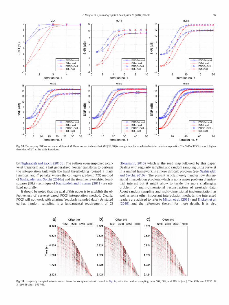
To offer more insights into the performance of POCS versus IST, 6experiments have been carried out after 5, 10, 20, 35, 50, and 80 iter-ations respectively. These experiments are based on the same geo-physical data as Fig. 9 with 40% random missing traces. Theirvarying SNR curves are shown in Fig. 10. Large iteration number Mimplies that we divide the threshold range [τmin,τmax] into finer stepsize. It is deserved to note that a slight increment of M can improvethe interpolation greatly when M is small; however, too large Mdoes not mean better recovery, and improves the result very little.Our experience on different geophysical data sets indicates thatM∈ [30,50] is enough to achieve a desirable interpolation in practice.As a matter of fact, a reasonable and moderate iteration number M isvery important, especially for very large scale applications. This hasbeen noted by many researchers, such as Fomel (2007) in his shapingregularization. It happens that Fomel and Jin (2009) even suggestedanother decreasing manner of regularization technique within asmall number of iterations. And our results are well in accordancewith this argument.

From the SNR curves in Fig. 10, it is surprising to find that the SNR ofPOCS is much higher than that of IST at the early iterations. In fact, it is anatural result because we use zeros to initialize d(k) for both POCS andIST. It always holds that PΛd

(k+1)=dobs,∀k in POCS method (cf.Eq. (14)) but not in ISTmethod. Noticing thatwe take the second largestcurvelet coefficient as the threshold (λk≈λmaxwhen k is very small), al-most all of the curvelet coefficients are thrown away, leading to toomany negligible values in d(k+1) such that ‖d‖2≈‖d−dk+1‖2 andSNR≈0 (cf. Eqs. (7), (10) and (20)). It seems that at the early iterations,to obtain comparable performance of interpolation as POCS, a betterthresholding strategy is required in the IST method. For moderate M,when k→M, the IST method can achieve the same performance as thePOCS algorithm, as shown in Fig. 10. This is easy to understand in con-sideration of Eq. (13).

As can be seen from the above, curvelet-based POCS with hardthresholding scheme is superior to other choices. Now we considertwo scenarios using this scheme. One scenario using random

2 All the remaining figures are the symmetric clipped data for the convenience ofdisplaying softer seismic events. We even employ the SNR measure to quantify the re-construction behavior of different methods.

Fig. 6. Interpolated results of the synthetic seismic data. (a) Interpolated result of POCS+hard thresholding, SNR=12.3057 dB. (b) Interpolated result of IST+hard thresholding,SNR=8.39441 dB. (c) Interpolated result of POCS+soft thresholding, SNR=6.808 dB. (d) Interpolated result of IST+soft thresholding, SNR=2.84215 dB. (a′–d′) The correspondingdifferences between Fig. 5a and panels a–d of this figure.

95P. Yang et al. / Journal of Applied Geophysics 79 (2012) 90–99

decimating rates 50%, 60%, and 70%, is plotted in Fig. 11. The interpo-lated seismic records are shown in Fig. 12. This result indicates thatthis method gains less SNR with too much random missing traces. Itis important to note that we only test our method in low dimensionalcases with only individual shot record. It is necessary to implementthe curvelet-based POCS with hard thresholding scheme in higherdimensional cases and many shots for more performanceimprovements.

The other scenario is the data with a gap. The motivation of de-signing such scenario is clear: in the process of real data acquisition,we always encounter the cases such as some regions where surveylines can not traverse, for example, a river, a lake or a mountain in aplain. This implies that we can only obtain seismic records includinglarge missing gaps, as plotted in Fig. 13a. Fig. 13b displays our

Fig. 7. One shot record from the real marine data set. (a) The complete data set, 430 traces,this data as the reference signal to compute the SNR behavior in the remaining article. (b) Raimated data with 40% missing traces, SNR=3.82511 dB.

reconstructed seismic record. Visually, the missing part has been re-covered to some extent. The difference between our interpolated re-sult and the complete data in Fig. 7a is shown in Fig. 13c. It seemsthat however, this method even fails because there still exist manyresidual traces which are not recovered. As a matter of fact, one fun-damental requirement of our method is random sampling. It is notapplicable to handle the regularly sampled seismic record and thesampled data with overlarge missing gaps.

6. Concluding remarks

Obviously, the mathematical framework in this article is general,not only restricted to the Fourier and curvelet transforms. In fact,many related approaches have been reported in the literature.

512 samples in each trace, the spatial interval=12.5 m, merely 0.124–2.124 s. We usendomly decimated data with 20% missing traces, SNR=7.32728 dB. (c) Randomly dec-

Fig. 8. Interpolated results of 20% missing marine data. (a) Interpolated result of POCS+hard thresholding, SNR=20.2571 dB. (b) Interpolated result of IST+hard thresholding,SNR=20.2571 dB. (c) Interpolated result of POCS+soft thresholding, SNR=19.5772 dB. (d) Interpolated result of IST+soft thresholding, SNR=19.5769 dB. (a′–d′) The corre-sponding differences between Fig. 7a and panels a–d of this figure.

96 P. Yang et al. / Journal of Applied Geophysics 79 (2012) 90–99

Sacchi et al. (1998) presented high-resolution discrete Fourier trans-form to perform the task of interpolation and extrapolation, utilizinga Cauchy–Gaussian a priori regularizer. Liu and Sacchi (2004)

Fig. 9. Interpolated results of 40% missing marine data. (a) Interpolated result of POCS+haSNR=14.5644 dB. (c) Interpolated result of POCS+soft thresholding, SNR=13.0042 dB. (sponding differences between Fig. 7a and Fig. 8a–d.

designed a minimum weighted norm interpolation (MWNI) algo-rithm, using weighted norm on the Fourier coefficients to stabilizethis geophysical inverse problem. This work was developed further

rd thresholding, SNR=14.5644 dB. (b) Interpolated result of IST+hard thresholding,d) Interpolated result of IST+soft thresholding, SNR=13.0041 dB. (a′–d′) The corre-

1 2 3 4 5−1

0

1

2

3

4

5

6

7

Iteration no. #

SN

R (

dB)

M=5

POCS−HardIST−HardPOCS−SoftIST−Soft

0 2 4 6 8 10−2

0

2

4

6

8

10

12

Iteration no. #

SN

R (

dB)

M=10

POCS−HardIST−HardPOCS−SoftIST−Soft

0 5 10 15 20−2

0

2

4

6

8

10

12

14

Iteration no. #

SN

R (

dB)

M=20

POCS−HardIST−HardPOCS−SoftIST−Soft

0 5 10 15 20 25 30 35−2

0

2

4

6

8

10

12

14

16

Iteration no. #

SN

R (

dB)

M=35

POCS−HardIST−HardPOCS−SoftIST−Soft

0 10 20 30 40 50−2

0

2

4

6

8

10

12

14

16

Iteration no. #

SN

R (

dB)

M=50

POCS−HardIST−HardPOCS−SoftIST−Soft

0 20 40 60 80−2

0

2

4

6

8

10

12

14

16

Iteration no. #

SN

R (

dB)

M=80

POCS−HardIST−HardPOCS−SoftIST−Soft

Fig. 10. The varying SNR curves under different M. These curves indicate thatM∈ [30,50] is enough to achieve a desirable interpolation in practice. The SNR of POCS is much higherthan that of IST at the early iterations.

97P. Yang et al. / Journal of Applied Geophysics 79 (2012) 90–99

by Naghizadeh and Sacchi (2010b). The authors even employed a cur-velet transform and a fast generalized Fourier transform to performthe interpolation task with the hard thresholding (coined a maskfunction) and ‘2 penalty, where the conjugate gradient (CG) methodof Naghizadeh and Sacchi (2010a) and the iterative reweighted least-squares (IRLS) technique of Naghizadeh and Innanen (2011) are uti-lized naturally.

It should be noted that the goal of this paper is to establish the ef-fectiveness of curvelet-based POCS interpolation method. Clearly,POCS will not work with aliasing (regularly sampled data). As statedearlier, random sampling is a fundamental requirement of CS

Fig. 11. Irregularly sampled seismic record from the complete seismic record in Fig. 7a, w2.1299 dB and 1.5557 dB.

(Herrmann, 2010) which is the road map followed by this paper.Dealing with regularly sampling and random sampling using curveletin a unified framework is a more difficult problem (see Naghizadehand Sacchi, 2010a). The present article merely handles low dimen-sional interpolation problem, which is not a major problem of indus-trial interest but it might allow to tackle the more challengingproblem of multi-dimensional reconstruction of prestack data.About random sampling and multi-dimensional implementation, aswell as some other important interpolation methods, the interestedreaders are advised to refer to Milton et al. (2011) and Trickett et al.(2010) and the references therein for more details. It is also

ith the random sampling rates 50%, 60%, and 70% in (a–c). The SNRs are 2.7635 dB,

Fig. 12. Interpolation from the missing traces in Fig. 11, using curvelet-based POCS with hard thresholding. (a–c) The interpolated results of Fig. 11a–c. Their SNRs are 11.9193 dB,10.2242 dB and 7.6424 dB, respectively. (a′–c′) The corresponding difference between the original complete data in Fig. 7a and our interpolation.

98 P. Yang et al. / Journal of Applied Geophysics 79 (2012) 90–99

important to point out that random sampling brings noisy spectrum,and regularly sampling produces aliased spectrum, which has beenout of the scope of our method.

As a summary, we would like to stress that our curvelet-basedPOCS interpolation method follows a sparseness-promoting approachthat is different from the previous contributions of many researchers.Even though soft thresholding is advocated in the IST algorithm byHennenfent and Herrmann (2005), Herrmann et al. (2007) andHerrmann (2010), POCS with hard thresholding scheme seemsmore appealing in practice, especially when we intend to carry outfew iterations to obtain a desirable reconstructed result.

Fig. 13. Interpolation with large gaps. (a) The incomplete seismic record including large gabetween (b) and Fig. 7a.

Acknowledgments

This work is supported by National Natural Science Foundation ofChina (40730424, 40674064) and National Science and TechnologyMajor Project (2008ZX05023-005-005, 2008ZX05025-001-009). Wewish to thank the authors of SeismicLab (http://www-geo.phys.ualberta.ca/saig/SeismicLab) and CurveLab (http://www.curvelet.org/) for their free available codes. We are grateful for the largeamount of valuable comments from Dirk J. Eric Verschuur and anoth-er anonymous reviewer, which lead to substantial improvements andmore awareness about the related references in this paper.

ps, SNR=8.5437 dB. (b) Our interpolated result, SNR=10.5240 dB. (c) The difference

99P. Yang et al. / Journal of Applied Geophysics 79 (2012) 90–99

References

Abma, R., Kabir, N., 2006. 3D interpolation of irregular data with a POCS algorithm.Geophysics 71, E91–E97.

Blumensath, T., Davies, M., 2008. Iterative thresholding for sparse approximations.Journal of Fourier Analysis and Applications 14, 629–654.

Blumensath, T., Davies, M., 2009. Iterative hard thresholding for compressed sensing.Applied and Computational Harmonic Analysis 27, 265–274.

Cai, J., Chan, R., 2008. A framelet-based image inpainting algorithm. Applied and Com-putational Harmonic Analysis 1–21.

Candès, E., 2006. Compressive sampling. Proceedings of the International Congress ofMathematicians, Citeseer, pp. 1433–1452.

Candès, E., Demanet, L., 2005. The curvelet representation of wave propagators is opti-mally sparse. Communications on Pure and Applied Mathematics 58, 1472–1528.

Candès, E., Donoho, D., 1999. Curvelets: a surprisingly effective nonadaptive represen-tation for objects with edges. In: Cohen, A., Rabut, C., Schumaker, L. (Eds.), Curveand Surface Fitting: Saint-Malo. Vanderbilt Univ. Press.

Daubechies, I., Defrise, M., De Mol, C., 2004. An iterative thresholding algorithm forlinear inverse problems with a sparsity constraint. Communications on Pure andApplied Mathematics 57, 1413–1457.

Donoho, D., 2006. Compressed sensing. IEEE Transactions on Information Theory 52,1289–1306.

Fomel, S., 2007. Shaping regularization in geophysical-estimation problems. Geophys-ics 72, R29–R36.

Fomel, S., Jin, L., 2009. Time-lapse image registration using the local similarity attribute.Geophysics 74, A7–A11.

Gao, J., Chen, X., Li, J., Liu, G., Ma, J., 2010. Irregular seismic data reconstruction based onexponential threshold model of POCS method. Applied Geophysics 7, 229–238.

Gao, J., Sacchi, M., Chen, X., 2011. Convergence improvement and noise attenuationconsiderations for POCS reconstruction. Proceedings of the EAGE 73th Conference.

Guleryuz, O., 2006a. Nonlinear approximation based image recovery using adaptivesparse reconstructions and iterated denoising—part I: theory. IEEE Transactionson Image Processing 15, 539–554.

Guleryuz, O., 2006b. Nonlinear approximation based image recovery using adaptivesparse reconstructions and iterated denoising—part II: adaptive algorithms. IEEETransactions on Image Processing 15, 555–571.

Gulunay, N., 2003. Seismic trace interpolation in the Fourier transform domain. Geo-physics 68, 355–369.

Hennenfent, G., Herrmann, F., 2005. Sparseness-constrained data continuation withframes: applications to missing traces and aliased signals in 2/3d. ExpandedAbstracts, SEG, Tulsa.

Hennenfent, G., Herrmann, F., 2006. Seismic denoising with nonuniformly sampledcurvelets. Computing in Science & Engineering 8, 16–25.

Hennenfent, G., Herrmann, F., 2007. Irregular sampling: from aliasing to noise. EAGE69th Conference & Exhibition.

Herrmann, F., 2003. Optimal seismic imaging with curvelets. SEG Expanded Abstracts.Herrmann, F., 2010. Randomized sampling and sparsity: getting more information

from fewer samples. Geophysics WB173–WB187.Herrmann, F.J., 2004. Curvelet imaging and processing: an overview. CSEG National

Convention.Herrmann, F.J., Böniger, U., Verschuur, D.J.E., 2007. Non-linear primary-multiple sepa-

ration with directional curvelet frames. Geophysical Journal International 170,781–799.

Kabir, M., Verschuur, D., 1995. Restoration of missing offsets by parabolic radon trans-form. Geophysical Prospecting 43, 347–368.

Lin, T.T.Y., Herrmann, F.J., 2007. Compressed wavefield extrapolation. Geophysics 72,SM77–SM93.

Liu, B., Sacchi, M., 2004. Minimum weighted norm interpolation of seismic records.Geophysics 69, 1560–1568.

Loris, I., Douma, H., Nolet, G., Daubechies, I., Regone, C., 2010. Nonlinear regularizationtechniques for seismic tomography. Journal of Computational Physics 229,890–905.

Milton, A., Trickett, S., Burroughs, L., 2011. Reducing acquisition costs with randomsampling and multidimensional interpolation. SEG San Antonio 2011 AnnualMeeting.

Naghizadeh, M., Innanen, K., 2011. Seismic data interpolation using a fast generalizedFourier transform. Geophysics 76, V1–V10.

Naghizadeh, M., Sacchi, M.D., 2007. Multistep autoregressive reconstruction of seismicrecords. Geophysics 72, V111–V118.

Naghizadeh, M., Sacchi, M.D., 2010a. Beyond alias hierarchical scale curvelet interpola-tion of regularly and irregularly sampled seismic data. Geophysics 75,WB189–WB202.

Naghizadeh, M., Sacchi, M.D., 2010b. On sampling functions and Fourier reconstructionmethods. Geophysics 75, WB137–WB151.

Neelamani, R.N., Krohn, C.E., Krebs, J.R., Romberg, J.K., Deffenbaugh, M., Anderson, J.E.,2010. Efficient seismic forward modeling using simultaneous random sources andsparsity. Geophysics 75, WB15–WB27.

Porsani, M.J., 1999. Seismic trace interpolation using half-step prediction filters. Geo-physics 64, 1461–1467.

Sacchi, M., 1997. Reweighting strategies in seismic deconvolution. Geophysical JournalInternational 129, 651–656.

Sacchi, M., Ulrych, T., 1995. High-resolution velocity gathers and offset space recon-struction. Geophysics 60, 1169–1177.

Sacchi, M., Ulrych, T., Walker, C., 1998. Interpolation and extrapolation using a high-resolution discrete Fourier transform. IEEE Transactions on Signal Processing 46,31–38.

Spitz, S., 1991. Seismic trace interpolation in the F–X domain. Geophysics 56, 785–794.Starck, J., Elad, M., Donoho, D., 2005. Image decomposition via the combination of

sparse representations and a variational approach. IEEE Transactions on Image Pro-cessing 14, 1570–1582.

Thorson, J.R., Claerbout, J.F., 1985. Velocity-stack and slant-stack stochastic inversion.Geophysics 50, 2727–2741.

Tian, B., Sclabassi, R., Hsu, J., Liu, Q., Pon, L., Li, C., Sun, M., 2004. POCS supperresolutionimage reconstruction using wavelet transform. ISPACS 2004., IEEE, pp. 67–70.

Trad, D., Ulrych, T., 2002. Accurate interpolation with high-resolution time-variantRadon transforms. Geophysics 67, 644–656.

Trad, D., Ulrych, T., Sacchi, M., 2003. Latest views of the sparse radon transform.Geophysics 68, 386.

Trickett, S., Burroughs, L., Milton, A., Walton, L., Dack, R., 2010. Rank-reduction-basedtrace interpolation. SEG Denver 2010 Annual Meeting.

Wang, Y., 2002. Seismic trace interpolation in the fxy domain. Geophysics 67,1232–1239.

Wang, Y., 2003. Sparseness-constrained least-squares inversion: application to seismicwave reconstruction. Geophysics 68, 1633–1638.

Zwartjes, P., Gisolf, A., 2007. Fourier reconstruction with sparse inversion. GeophysicalProspecting 55, 199–221.

Zwartjes, P.M., Sacchi, M.D., 2007. Fourier reconstruction of nonuniformly sampled,aliased seismic data. Geophysics 72, V21–V32.