Finite element time domain modeling of controlled-Source electromagneticdata with a hybrid boundary condition

Hongzhu Cai, Xiangyun Hu, Bin Xiong, Esben Auken, Muran Han,Jianhui Li

PII: S0926-9851(17)30087-3DOI: doi:10.1016/j.jappgeo.2017.08.005Reference: APPGEO 3321

To appear in: Journal of Applied Geophysics

Received date: 19 January 2017Revised date: 27 July 2017Accepted date: 16 August 2017

Please cite this article as: Cai, Hongzhu, Hu, Xiangyun, Xiong, Bin, Auken, Esben,Han, Muran, Li, Jianhui, Finite element time domain modeling of controlled-Sourceelectromagnetic data with a hybrid boundary condition, Journal of Applied Geophysics(2017), doi:10.1016/j.jappgeo.2017.08.005

This is a PDF file of an unedited manuscript that has been accepted for publication.As a service to our customers we are providing this early version of the manuscript.The manuscript will undergo copyediting, typesetting, and review of the resulting proofbefore it is published in its final form. Please note that during the production processerrors may be discovered which could affect the content, and all legal disclaimers thatapply to the journal pertain.

ACC

EPTE

D M

ANU

SCR

IPT

ACCEPTED MANUSCRIPT

Finite element time domain modeling of

controlled-Source electromagnetic data with a hybrid

boundary condition

Hongzhu Caia, Xiangyun Hub, Bin Xiongc, Esben Aukend, Muran Hane,Jianhui Lib

aAarhus University, Department of Geoscience, Aarhus, Denmark (Previously withTechnoImaging, Salt Lake City, Utah, US)

bChina University of Geosciences, Institute of Geophysics and Geomatics, Wuhan, ChinacCollege of Earth Sciences, Guilin University of Technology, Guilin, Guangxi, China 541004

dAarhus University, Department of Geoscience, Aarhus, DenmarkeUniversity of Utah, Salt Lake City, Utah, USA 84112

Abstract

We implemented an edge-based finite element time domain (FETD) modeling

algorithm for simulating controlled-source electromagnetic (CSEM) data. The

modeling domain is discretized using unstructured tetrahedral mesh and we con-

sider a finite difference discretization of time using the backward Euler method

which is unconditionally stable. We solve the diffusion equation for the electric

field with a total field formulation. The finite element system of equation is

solved using the direct method. The solutions of electric field, at different time,

can be obtained using the effective time stepping method with trivial computa-

tion cost once the matrix is factorized. We try to keep the same time step size for

a fixed number of steps using an adaptive time step doubling (ATSD) method.

The finite element modeling domain is also truncated using a semi-adaptive

method. We proposed a new boundary condition based on approximating the

total field on the modeling boundary using the primary field corresponding to

a layered background model. We validate our algorithm using several synthetic

model studies.

Email addresses: caihongzhu@hotmail.com (Hongzhu Cai), xyhu@cug.edu.cn (XiangyunHu), hsiungbin@hotmail.com (Bin Xiong), esben.auken@geo.au.dk (Esben Auken),muran.han@gmail.com (Muran Han), ljhiiicumt@126.com (Jianhui Li)

Preprint submitted to Journal of LATEX Templates August 17, 2017

ACC

EPTE

D M

ANU

SCR

IPT

ACCEPTED MANUSCRIPT

Keywords: Electromagnetics, marine geophysics, time domain, finite element,

backward Euler, direct solver

1. Introduction

The controlled-source electromagnetic (CSEM) methods can be used to pro-

vide a resistivity map of the subsurface structure in geophysical exploration

(Mulder et al., 2007). This method has been widely adopted in the applica-

tion of mineral exploration, environmental study, ground water exploration and

oil reservoir identification (Fitterman and Stewart, 1986; Ward and Hohmann,

1988; Kamenetsky, 1997; Oh et al., 2015; Persova et al., 2015; Beka et al., 2017).

Recently, we also observed a strong interest of using such method in offshore

exploration for hydrocarbon reservoir (Constable and Srnka, 2007; Wang et al.,

2017). There exist two main categories of CSEM methods: the frequency do-

main CSEM method and the time domain CSEM method (Ward and Hohmann,

1988; Zhdanov, 2009).

The frequency domain CSEM method has been widely applied in both land

and marine environment to map the resistivity structures (Ward and Hohmann,

1988; Connell and Key, 2013). However, the frequency domain electromag-

netic (EM) signal is usually dominated by the primary field for typical CSEM

survey configurations and this fact leads to a relative small target response

(Ward and Hohmann, 1988). Moreover, the air-wave is dominant in land and in

shallow marine environments, especially at long source-receiver offsets (Mulder et al.,

2007; Key, 2012a; Connell and Key, 2013). The airwave is also coupled with the

earth structure which makes the airwave decomposition methods technically dif-

ficult (Connell and Key, 2013). The time-domain electromagnetic methods is

suggested to overcome these difficulties since the airwave arrives at the early

times and the target response from the earth’s structures arrives at relatively

late-time (Mulder et al., 2007; Connell and Key, 2013; Weiss, 2007; Li, 2010;

Jang and Kim, 2015; Sridhar et al., 2017). In addition, the time-domain CSEM

method collect data in a similar way to seismic method. The EM data can poten-

2

ACC

EPTE

D M

ANU

SCR

IPT

ACCEPTED MANUSCRIPT

tially be integrated with seismic data and the well-developed seismic data pro-

cessing techniques (e.g., stacking, filtering) can be applied (Strack and Allegar,

2008). It is beneficial to integrate the EM data with seismic data in order to

overcome the lower resolution of EM data arising from the diffusive nature of

the method (Strack and Allegar, 2008).

Unlike seismic data, the EM signals are diffusive in the conductive earth

medium and the direct interpretation of the time-domain EM data is challeng-

ing which makes inversion of the data necessary (Mulder et al., 2007). For

robust inversion of time-domain EM data, we need an efficient and accurate

modeling algorithm (Mulder et al., 2007; Yang et al.,, 2014). The better and

more accurate we can simulate the time domain response for realistic earth

models, the more useful geological information we can extract from the signals

(Sugeng et al., 1993). Comparing to the conventional approach which is to cal-

culate the time-domain response from the transformation of frequency domain

solution (Everett and Edwards, 1993; Mulder et al., 2007; Ralph-Uwe et al., 2008),

the direct time stepping of Maxwell’s equation for electric and magnetic field

is preferred, in certain applications, due to its accuracy and computational effi-

ciency (Jin, 2002, 2014; Wang and Hohmann, 1993).

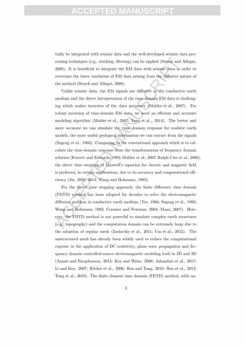
For the direct time stepping approach, the finite difference time domain

(FDTD) method has been adopted for decades to solve the electromagnetic

diffusion problem in conductive earth medium (Yee, 1966; Sugeng et al., 1993;

Wang and Hohmann, 1993; Commer and Newman, 2004; Maaø, 2007). How-

ever, the FDTD method is not powerful to simulate complex earth structures

(e.g., topography) and the computation domain can be extremely large due to

the adoption of regular mesh (Zaslavsky et al., 2011; Um et al., 2012). The

unstructured mesh has already been widely used to reduce the computational

expense in the application of DC resistivity, plane wave propagation and fre-

quency domain controlled-source electromagnetic modeling both in 2D and 3D

(Ansari and Farquharson, 2014; Key and Weiss, 2006; Jahandari et al., 2017;

Li and Key, 2007; Rucker et al., 2006; Ren and Tang, 2010; Ren et al., 2013;

Tang et al., 2010). The finite element time domain (FETD) method, with un-

3

ACC

EPTE

D M

ANU

SCR

IPT

ACCEPTED MANUSCRIPT

structured mesh, was proposed to overcome these difficulties in electric engi-

neering (Jin, 2002, 2014). This method was recently introduced to the geophys-

ical community for simulating electromagnetic diffusion problems (Um, 2011;

Um et al., 2012; Yin et al., 2016). However, the FETD method requires solv-

ing the sparse system of equations at each time stepping for either the explicit

or implicit scheme. Fortunately, the developments of computer hardware and

the modern direct solver algorithms make it possible to factorize the sparse

finite element system of equations efficiently (Jin, 2002, 2014). For the same

time stepping size, the FETD stiffness matrix stays unchanged (Jin, 2002, 2014;

Um et al., 2012). As a result, the matrix factorization can be reused for the

direct solution of the system of equations (Jin, 2002, 2014; Um et al., 2012).

In this paper, we consider the FETD formulation with adaptive time step dou-

bling proposed by Um et al. (2012). Within the framework of this approach,

the time step size increases with time and the computation cost can be reduced

significantly.

For either FDTD or FETD modeling, the Dirichlet boundary is usually

adopted (Wang and Hohmann, 1993; Um et al., 2012). For a typical geophysical

application, the modeling domain size needs to be tens or hundred km, in each

dimension (Um, 2011; Um et al., 2012). The more advanced absorbing bound-

ary conditions (ABC) and the perfectly matched layer (PML) were commonly

used to truncate the computation regions in electric engineering (Jin, 2002, 2014;

Feng and Liu, 2014). We have observed some trials of using these boundary con-

ditions for geophysical application (Wang and Tripp, 1996; Chen et al.,, 1997).

However, these boundary conditions are still not quite applicable to lossy me-

dia (Wang and Tripp, 1996; Chen et al.,, 1997) and the implementation of these

boundary condition requires significant effort (Jin, 2002, 2014). To address this

problem, we approximate the total electric field at different time stage by the

primary field corresponding to a layered background conductivity model which

can best approximate the full 3D structure (Cai et al., 2017). The primary

field in the time domain, for the layered background model, is calculated from

the transformation of the frequency domain data obtained using fast Hankel

4

ACC

EPTE

D M

ANU

SCR

IPT

ACCEPTED MANUSCRIPT

transform (Anderson, 1989; Guptasarma and Singh, 1997; Ward and Hohmann,

1988; Kirkegaard and Auken, 2015). However, the calculated time domain pri-

mary field is not accurate for the very earlier stage (Li, 2016). We propose to

use the conventional Dirichlet boundary condition with a large modeling domain

for the very early modeling stage. Once the FETD solution on the truncated

modeling domain boundary produces similar result as the primary field on this

boundary, the algorithm will switch to the hybrid boundary condition with the

truncated modeling domain. With this method, the computation cost can be

reduced significantly.

In the rest part of this paper, we will demonstrate our developed method

and algorithm using several typical synthetic model studies.

2. Finite Element Time Domain Discretization of Maxwell’s Equation

Consider the quasi-static approximation, we can write the Maxwell’s equa-

tion in time domain as follows (Ward and Hohmann, 1988; Um et al., 2012):

∇×E = −µ∂H

∂t(1)

∇×H = je + Js (2)

where E andH are electric and magnetic fields. Js is source current density and

je is the induction current in the conductive earth medium (Ward and Hohmann,

1988; Zhdanov, 2009):

je = σE (3)

Here, we consider a general anisotropic earth in our formulation by introducing

the electric conductivity tensor σ (Cai et al., 2017).

We can eliminate the magnetic field term from the Maxwell’s equation and

obtain the following diffusion equation (Um et al., 2012):

∇×∇× E(t) + µ∂je(t)

∂t= −µ

∂Js(t)

∂t(4)

5

ACC

EPTE

D M

ANU

SCR

IPT

ACCEPTED MANUSCRIPT

Fig. 1. A tetrahedral element with edge and node definition (Cai et al., 2017).

By substituting (3) into (4), we arrive at the following equation which is ready

to be solved using FETD method:

∇×∇× E(t) + µσ∂E(t)

∂t= −µ

∂Js(t)

∂t(5)

We consider the edge-based finite element (Nedelec, 1980; Jin, 2002, 2014)

with a total field formulation and unstructured tetrahedral mesh, as shown in

Fig. 1. For the edge-based finite element method, the electric field, at different

time stage, is assigned on the element edges and the field inside the element can

be calculated from the linear combination of the field on the edges:

Ee(t) =6∑

i=1

NeiE

ei (t). (6)

We apply the Galerkin finite element analysis to (5) and obtain a finite element

system of equations as follows (Jin, 2002, 2014):

KE(t) + µσM∂E(t)

∂t= −µM

∂Js(t)

∂t(7)

where the stiffness matrix K and M are defined as:

Keij =

∫

Ωe

(∇×Nei ) ·(∇×Ne

j

)dv, (8)

Meij =

∫

Ωe

Nei ·N

ejdv, (9)

6

ACC

EPTE

D M

ANU

SCR

IPT

ACCEPTED MANUSCRIPT

and Ωe indicates the domain for each element.

We consider a backward Euler scheme, which is unconditionally stable, to

calculate the time derivative term in (7) (Ascher and Greif, 2011; Jin, 2002,

2014; Haber, 2014):∂E(t)

∂t≈

E(t)−E(t−∆t)

∆t(10)

where ∆t is the time-step size.

By substituting this equation into (7), we can obtain:

KE(t) +µσ

∆tME(t) =

µσ

∆tME(t−∆t)− µM

∂Js(t)

∂t(11)

With known initial condition, source waveform and proper boundary condition,

the electric field at any time can be obtained by solving (11) in a time stepping

manner.

We can further write (11) in a simple form as follows:

AE(t) = b (12)

where:

A = K +µσ

∆tM, (13)

and

b =µσ

∆tME(t−∆t)− µM

∂Js(t)

∂t. (14)

3. Hybrid Boundary Condition

Before one can solve the system of equations (12), proper boundary condition

needs to be applied to specify the electromagnetic field on the boundary of the

modeling domain in order to get a unique solution (Ward and Hohmann, 1988).

The homogeneous Dirichlet boundary condition:

E(t)Ωs= 0, (15)

which assumes the electromagnetic field vanishes on the boundary at all time

stage, is the mostly used one due to its simplicity. This type of simple bound-

ary condition generally works effectively for the secondary field formulation

7

ACC

EPTE

D M

ANU

SCR

IPT

ACCEPTED MANUSCRIPT

considering that the secondary field is relatively small, the modeling domain is

reasonably large enough and its boundary is far away from the region filled with

anomalous conductivity (Zhdanov, 2009; Silva et al., 2012; Um, 2011; Um et al.,

2012). Due to these reasons, the homogeneous Dirichlet boundary has been

widely used for the numerical modeling of CSEM data using finite difference,

finite volume and finite element methods (Badea et al., 2001; Streich, 2009;

Schwarzbach et al., 2011; Um et al., 2012; Silva et al., 2012; Cai et al., 2014).

However, to use the homogeneous Dirichlet boundary condition for the total

field formulation, one has to set a relatively large modeling domain (Ward and Hohmann,

1988; Jahandari and Farquharson, 2014; Haber et al., 2007; Haber, 2014). One

need to note that the size of a modeling domain also depends on the moment of

the source (Cai et al., 2017). The same grid may work for a survey with lower

source moment but it may not work anymore if one increase the source moment.

In addition, the electric field on the modeling domain boundary also changes

with time for FETD modeling (Jin, 2002, 2014). As a result, the application of

the conventional Dirichlet boundary condition can be problematic.

We propose to use a new boundary condition which approximate the to-

tal field on the domain boundary by the primary field. We define a layered

background conductivity model which can best approximate the actual 3D con-

ductivity. As a result, the background model contains the averaged conductivity

information of the actual 3D model. We define the primary field as the electro-

magnetic response excited by the source in the background conductivity model.

In our algorithm, we can either specify this background conductivity model in

input file or let the algorithm calculate it automatically. Based on our numerical

tests, we find that this type of boundary condition works much more efficiently

than the homogeneous Dirichlet boundary condition. The size of the model-

ing domain can be reduced dramatically. In addition, the size of the modeling

domain becomes irrelevant with the source moment.

Fig. 2 shows a 2D illustration of this hybrid boundary condition (our method

is actually for a general 3D case). For the conventional homogeneous Dirichlet

boundary condition, we have to use a large domain A with boundary of ΩA.

8

ACC

EPTE

D M

ANU

SCR

IPT

ACCEPTED MANUSCRIPT

Fig. 2. 2D illustration of modeling domain truncation and the hybrid boundary

condition.

Instead, we can use a small modeling domain B with boundary of ΩB . In this

case, we approximate the time-domain electric field on ΩB by the primary field

corresponding to a layered background model.

This approach has been demonstrated to be effective for frequency domain

EM modeling (Cai et al., 2017) where the optimized truncation domain ΩB

can be decided in a semi-adaptive manner (Cai et al., 2017). For a specific

frequency, we can start from a small modeling domain and gradually increase

the domain size. We can do forward modeling for these different domains (from

the smallest one) and terminate the process until the solution difference reaches

the tolerance. For one frequency, the solution for a small domain can be obtained

very quickly and the computation cost for this process is low (Cai et al., 2017).

However, this adaptive approach cannot be directly applied to time domain,

since the computational cost in each small domain is much more expensive than

for frequency domain modeling. In this paper, the size of the truncated domain

is obtained based on experience.

9

ACC

EPTE

D M

ANU

SCR

IPT

ACCEPTED MANUSCRIPT

As we mentioned before, the calculated time domain primary field on the

boundary of the truncated domain is not accurate for the earlier stage due to

the limitation of digital filter used for the frequency-time domain transformation

(Key, 2012b; Li, 2016). As a result, one need to be cautious to apply such hybrid

boundary condition. To overcome this problem, we decide to use a dual domain

modeling method as shown in Fig. 2. For the earlier stage, we use a large

domain A with homogeneous Dirichlet boundary condition. Once the difference

between the primary field and the FETD solution, simulated with homogeneous

Dirichlet boundary condition and larger domain, on boundary ΩB is within the

preselected tolerance ǫ, we will switch to the hybrid boundary condition with a

smaller modeling domain of B.

4. Initial Condition and Solution of FETD System

Before applying the time stepping process, we need to specify the initial

condition based on the source waveform. In this paper, we adopt the impulse

source which is approximated by a Gaussian function as shown in Fig. 3. For

this type of source waveform, a zero initial condition can be used (Um et al.,

2012). Actually, our algorithm can take the arbitrary waveform as input. The

initial time stepping size depends on the discretization of the source waveform.

With the discussed initial and boundary condition, the system of equation (12)

is ready to be solved. It has been shown that we have to solve the system

at each step for FETD formulation (Jin, 2002, 2014). It will be unrealistic to

solve such system using iterative solver considering the number of time stepping

could be large (Jin, 2002, 2014; Um et al., 2012). It has been shown that the

FETD stiffness matrix stays the same if we use the same time stepping size of

∆t. In this scenario, it may be reasonable to use a direct solver since the matrix

factorization can be reused if we keep the same time stepping size (Jin, 2002,

2014; Oldenburg et al., 2012). In this paper, we use the direct solver package

SuiteSparse v4.5.3 with a MATLAB interface (Davis, 2006) to solve the system

of equations.

10

ACC

EPTE

D M

ANU

SCR

IPT

ACCEPTED MANUSCRIPT

0 0.1 0.2 0.3 0.4 0.5 0.6 0.7 0.8 0.9 1t(s) 10-6

0

0.5

1

1.5

2

2.5

3

3.5

4

A

106 Gaussian pulse

Fig. 3. Approximation of the impulse source waveform with Gaussian pulse.

However, the number of time steps will be significantly large if we keep

∆t unchanged since a small time stepping size is required in the earlier stage

(Um et al., 2012). To solve this problem, we consider an adaptive time stepping

doubling methods (Um et al., 2012) to gradually increase the time stepping size.

Within the framework of this approach, we keep the same time stepping size ∆t

for a fixed number of steps (e.g., 100 step) and then try to increase the time step

size to 2∆t. If the difference between the FETD solution for these two different

time step size is smaller than the tolerance, the time stepping doubling will

be accepted and vice versa (Um, 2011; Um et al., 2012). If the time stepping

doubling is rejected, the matrix factorization for the FETD matrix with step size

of 2∆t can still be saved for the next time stepping doubling trial. It has been

demonstrated that the time stepping process can be speeded up dramatically by

adopting the ATSD (adaptive time step doubling) method (Um et al., 2012).

5. Model Studies

In this section, we will validate the developed algorithm by several model

studies. For simplicity, we consider the electric dipole source. The more com-

plicated source geometry (e.g., long wire and loop) can be constructed from

integration of electric dipoles (Ward and Hohmann, 1988; Cai et al., 2017) and

11

ACC

EPTE

D M

ANU

SCR

IPT

ACCEPTED MANUSCRIPT

will be studied in the future. We first consider a halfspace model with the elec-

tric dipole source located at the air-earth interface such that the solution of

the EM signal at the receiver has a closed form. Following this, we consider a

3D anomaly embedded in the half space background. For the frequency-time

domain transformation, we use the method in Key (2012b) with 101 frequen-

cies uniformly spaced from 10−5 Hz to 105 Hz in logarithmic space. Finally,

we demonstrate our algorithm by the more realistic SEG marine salt model

with complex bathymetry. We run the algorithm on a PC desktop with 4 cores

(i7-6700K) and 64 GB memory.

5.1. Halfspace model

We first consider the electromagnetic diffusion in a halfspace earth, with the

resistivity of 500Ω ·m, excited by an electric dipole located at (−1000, 0, 0)m.

We use the same source waveform as shown in Fig. 3. The source waveform

discretization results in an initial time step size of 5 × 10−8s. We simulate the

electromagnetic response from t = 0 to t = 1s.

As mentioned, we use a dual modeling domain during this simulation. In the

earlier stage, we use a large modeling domain with a size of 50km×50km×50km.

Such relative large domain contains 312,551 elements and 371,328 edges. In the

late stage, we use a smaller modeling domain with the size of 4km×4km×4km.

The smaller domain (truncated domain) contains 68,705 elements and 81,358

edges. The homogeneous Dirichlet boundary condition and the proposed hybrid

boundary condition are applied to the larger and smaller modeling domain,

respectively. The total computation time is around 400 s for the dual-modeling

domain approach with the proposed hybrid boundary condition. However, it

takes around 25 minutes to finish the calculation if we choose the homogeneous

Dirichlet boundary condition with the large modeling domain. The total number

of time steps is 1773 with the ATSD method. Fig. 4 shows that the time step

size increases with time. The total number of steps would be 2 × 107 if we use

a uniform time step size of 5 × 10−8.

Fig. 5 shows the inline electric field on the earth’s surface calculated from an

12

ACC

EPTE

D M

ANU

SCR

IPT

ACCEPTED MANUSCRIPT

10 -6 10 -4 10 -2 10 0

t(s)

10 -7

10 -6

10 -5

10 -4

10 -3

t(s)

Fig. 4. Adaptive time step size for the halfspace model.

analytical solution (see equation (A.8)) and FETD method with the proposed

hybrid boundary condition at two different offsets. We can see that the FETD

solution compares well to the analytical solution in both earlier and late-time.

Fig. 6 shows the inline electric field on the earth’s surface calculated from the

analytical solution and the FETD method with the conventional zero Dirichlet

boundary condition at two different offsets. From this figure, we can clearly

see that the difference between the FETD solution and the analytical for late-

time, although we used a relative large modeling domain for the zero Dirichlet

boundary condition.

Fig. 7 shows the sparsity pattern of the FETD stiffness matrix for the model-

ing with conventional zero Dirichlet boundary condition and the hybrid bound-

ary condition. We can see that the number of non-zeros for the conventional zero

Dirichlet boundary condition case is almost 5 times as the case with the pro-

posed hybrid condition. It is clear that the computational expense and memory

cost can be reduced significantly by adopting this hybrid boundary condition. In

the meantime, the numerical accuracy is improved dramatically. Furthermore,

we want to emphasize that for the conventional zero Dirichlet boundary con-

13

ACC

EPTE

D M

ANU

SCR

IPT

ACCEPTED MANUSCRIPT

10 -4 10 -2 10 0

t(s)

10 -6

10 -4

10 -2

10 0

10 2

V/m

Offset=1000, z=0

AnalyticalFETD

10 -3 10 -2 10 -1 10 0

t(s)

10 -6

10 -4

10 -2

10 0

V/m

Offset=2000, z=0

Fig. 5. A comparison between the inline electric field component, Ex, calculated

from analytical solution and FETD method with the hybrid boundary condition for

the halfspace model at the offsets of 1000m and 2000 m.

14

ACC

EPTE

D M

ANU

SCR

IPT

ACCEPTED MANUSCRIPT

10 -4 10 -2 10 0

t(s)

10 -6

10 -4

10 -2

10 0

10 2

V/m

Offset=1000, z=0

AnalyticalFETD

10 -3 10 -2 10 -1 10 0

t(s)

10 -6

10 -4

10 -2

10 0

V/m

Offset=2000, z=0

Fig. 6. A comparison between the inline electric field component, Ex, calculated from

analytical solution and FETD method with the conventional zero Dirichlet boundary

condition for the halfspace model at the offsets of 1000m and 2000 m.

15

ACC

EPTE

D M

ANU

SCR

IPT

ACCEPTED MANUSCRIPT

Fig. 7. Panel a) shows the sparsity pattern of stiffness matrix for the FETD method

with the conventional zero Dirichlet boundary condition; panel b) shows the sparsity

pattern of stiffness matrix for the FETD method with the proposed hybrid boundary

condition. The parameter nz in each panel represents the number of no-zeros in the

stiffness matrix.

dition, the modeling domain also depends on the source moment. A modeling

domain works for small source moment may not work anymore if we increase

the source moment (Cai et al., 2017). However, within the framework of the

proposed hybrid boundary condition, the size of the domain truncation actually

does not depends on the source moment.

5.2. 3D model with flat surface

We now consider a 3D model with two anomalous bodies embedded in the

halfspace earth with a resistivity of 500Ω · m. Fig. 8 is an illustration of this

16

ACC

EPTE

D M

ANU

SCR

IPT

ACCEPTED MANUSCRIPT

500

1000

500

y(m)

0

-500 1000500

x(m)

0-500-1000

-1000

z(m

)

3D Model

0

Fig. 8. Illustration of the 3D model. The red cubes are the anomalous bodies. The

black dots represent the receivers while the red diamond shape in the left indicates

the location of the electric dipole source.

model. The size of these two anomalous bodies are 250m×250m×250m. The

resistivity of the left body is 1Ω·m while the resistivity of the right body is

0.2Ω·m. The center location of these two bodies are located at (−400, 100, 300)m

and (400, 0, 200)m, respectively. The x oriented electric dipole source is located

at (−1000, 0, 0)m.

We use the hybrid boundary condition for this model and the finite element

modeling domain is the same as the previous halfspace model. However, we

refined the mesh inside the anomalous bodies and the observation surface. The

tetrahedral mesh for the large domain contains 306, 908 elements and 361, 763

edges. The tetrahedral mesh for the truncated domain contains 185, 801 ele-

ments and 220, 408 edges. The total computation time for this model is around

10 minutes.

For comparison, we also compute the time domain response using the cosine

transform and the frequency domain response is calculated using a frequency

17

ACC

EPTE

D M

ANU

SCR

IPT

ACCEPTED MANUSCRIPT

FETD, t=0.25119 s

-500 0 500 1000x(m)

-1000

-500

0

500

1000

z(m

)

3

3.5

4

4.5

5

V/m

10-10

Cosine Transform, t=0.25119 s

-500 0 500 1000x(m)

-1000

-500

0

500

1000z(

m)

3

3.5

4

4.5

5

V/m

10-10

Fig. 9. FETD solution and the frequency domain transformed solution for the 3D

model with a flat surface. The arrows represent the direction of the electric field on

the surface.

domain FEM code (Cai et al., 2017). Fig. 9 shows the electric field, on the

earth’s surface at t≈0.25s, calculated with the FETD method and the cosine

transform, respectively. We can see that the FETD solution compares well with

the frequency-domain transformed result. Fig. 10 shows the electric field, at

t≈0.25s, on the vertical plane of y = 0.

Fig. 11 shows the time domain response of the electric field at the location of

(−400, 0, 0) m, which is directly above the left anomalous body. In this figure,

we also present the comparison between the FETD solution and the frequency

domain transformed result, at one station. We can see that the FETD solution

matches well with the frequency domain transformed solution at different time

stages. In addition, we compared the results with the halfspace response (dashed

black line). We can clearly see the distortion from the 3D bodies. At this

18

ACC

EPTE

D M

ANU

SCR

IPT

ACCEPTED MANUSCRIPT

Et, t=0.25119 s

-800 -600 -400 -200 0 200 400 600 800x(m)

200

400

600

800

1000

1200

1400

z(m

)

1

2

3

4

5

6

7

8

9

10

V/m

10-10

Fig. 10. FETD solution, for the 3D model with a flat surface, on the plane of y = 0.

The arrows represent the direction of the electric field on this plane.

19

ACC

EPTE

D M

ANU

SCR

IPT

ACCEPTED MANUSCRIPT

10-3 10-2 10-1 100

time(s)

10-10

10-8

10-6

10-4

10-2

V/m

Ex at (-400, 0, 0) m

FETD 3DCosine Transform 3D1D Analytical

Fig. 11. Time domain response of electric field at x = −400 m, y = 0 and z = 0.

sounding station, which is above the left anomalous body, the size of the body

is relative large comparing to the source-receiver offset, the EM response is

affected significantly by the target even in the late-time.

Fig. 12 shows the time domain response of the electric field at the location

of (1000, 0, 0) m. It shows the EM response for the case with and without 3D

anomaly. In the case of without 3D anomaly, the solution is calculated both

with the analytical method and FETD method (we use exact the same mesh

as the case with 3D anomaly). We see that the halfspace response calculated

from analytical solution (black dots) is almost identical with the solution from

the FETD method (solid blue line). By doing this comparison, we can further

validate that the selected mesh grid and modeling domain is proper and will

not cause artificial anomalies. The dashed red line in Fig. 12 represents the

EM response for the model with 3D anomalies. At this sounding station, the

source-receiver offset is relative much larger comparing to the dimension of the

3D anomalies and the receiver is at some distance from the anomalous bodies,

the 3D model response converges, as expected, to the halfspace response at

20

ACC

EPTE

D M

ANU

SCR

IPT

ACCEPTED MANUSCRIPT

late-time channels.

6. Realistic marine salt dome model

Finally, we consider a marine CSEM model with complex bathymetry and a

salt structure (Aminzadeh et al., 1996) that we used in our previous publication

(Cai et al., 2017). Fig. 13 shows an illustration of this model.

This model contains multiple geological layers characterized by resistivity

anisotropy. The resistivity of the seawater is 3.3Ω · m. The horizontal and

vertical resistivity of sediments are 1Ω · m and 1.25Ω · m, respectively. The

horizontal and vertical resistivity of the basement rock, underlie the sediments,

are 10Ω · m and 20Ω · m. The salt structure is resistive with a horizontal

and vertical resistivity of 100Ω · m and 500Ω · m, respectively. We consider

several x oriented electric dipole sources towed above the seafloor. Because

we adopt the direct solver, the matrix only needs to be factorized once for all

sources. As a result, the number of sources will not increase the calculation

time significantly. We will only show the results for the electric dipole source

located at (−4000, 0, 800) m. The source waveform is the same as the previous

models.

The optimized truncated modeling domain size is 16km×14km×14km and

the unstructured discretization of this truncated domain results in 548,419 el-

ements and 465,904 edges. The size of the large domain with homogeneous

Dirichlet boundary condition is 60km×60km×60km and the corresponding un-

structured mesh contains 691,169 elements and 813,504 edges. The total com-

putation for running this model is around 36 minutes. However, it takes around

2 hours to solve it with a large domain and the Dirichlet boundary condition.

In addition, the large domain with 813,504 edges almost reaches the limits of

the SuiteSparse solver.

Fig. 14 shows a comparison between the FETD solution and the transforma-

tion from the frequency domain result (Cai et al., 2017) at one receiver location.

We can see the FETD result compares well with the frequency domain trans-

21

ACC

EPTE

D M

ANU

SCR

IPT

ACCEPTED MANUSCRIPT

10-3 10-2 10-1

t(s)

10-10

10-9

10-8

10-7

10-6

10-5

V/m

Ex at (1000,0,0) m

FETD With No Anomaly1D AnalyticalFETD 3D

Fig. 12. Time domain response of electric field at x = 1000 m, y = 0 and z = 0.

22

ACC

EPTE

D M

ANU

SCR

IPT

ACCEPTED MANUSCRIPT

Fig. 13. SEG salt dome model with complex bathymetry. The lower panel shows the

surface discretization of the salt (Cai et al., 2017).

23

ACC

EPTE

D M

ANU

SCR

IPT

ACCEPTED MANUSCRIPT

100 101 102

t(s)

10-15

10-14

V/m

Ex, x=3000m

FETDCosine Transform

Fig. 14. A comparison between FETD solution and the frequency domain trans-

formed solution for the salt dome model, at x = 3000 and y = 0.

formed result for this complex model. The FETD solution also compares well

to the frequency domain transformed solution for all other receivers.

We also computed the total field with bathymetry but without the salt dome

response. Fig. 15 shows a comparison between the total field, layered back-

ground response and the total field without salt dome, at x = 3000 and y = 0.

From this figure, we can clearly see the distortion caused by bathymetry and

the salt dome from t = 1s to t = 10s.

We can normalize the total field by some background field to get the nor-

malized anomaly which can reflect the distortion from the target. We normalize

the total field by the layered background response and also by the bathymetry

background. We define the bathymetry background as the total field for the

model with bathymetry but without the salt dome. Fig. 16 shows a comparison

between these two different normalized anomalies. We can see that the normal-

ized anomaly can be overestimated without carefully considering the bathymetry

effects.

24

ACC

EPTE

D M

ANU

SCR

IPT

ACCEPTED MANUSCRIPT

100 101

t(s)

10-15

10-14

V/m

Ex, x=3000m

TotalLayered BackgroundTotal without salt

Fig. 15. The time domain response of the electric field, at x = 3000 and y = 0, for

different scenarios.

25

ACC

EPTE

D M

ANU

SCR

IPT

ACCEPTED MANUSCRIPT

100 101

t(s)

1

1.05

1.1

1.15

1.2

1.25

Rat

io

Total/Layered backgroundTotal/Bathymetry background

Fig. 16. Normalized anomaly of the time domain electric field, at x = 3000 and

y = 0, by different background field.

Finally, we calculate the time domain response for this model with isotropic

resistivity by setting the resistivity as the horizontal resistivity in all area.

Fig. 17 shows a comparison between the time domain response for this model

with isotropic and anisotropic resistivity. We can see that the time domain

response is distorted remarkably by the anisotropic effects.

7. Conclusions

We have developed a 3D edge-based finite element time domain model-

ing algorithm for solving electromagnetic diffusion problem in conductive earth

medium. The diffusive equation is discretized using a backward Euler scheme

which is unconditionally stable. The sparse system of equation is solved using

the direct method based on LU decomposition and as a result the matrix fac-

torization can be reused for the same time stepping size. We also consider an

adaptive time step doubling scheme to gradually increase the time step size. The

modeling domain is discretized using unstructured tetrahedral mesh to reduce

the size of the problem and simulate complex geometry.

26

ACC

EPTE

D M

ANU

SCR

IPT

ACCEPTED MANUSCRIPT

100 101 102

t(s)

10-15

10-14

V/m

Ex, x=3000m

Total AnisotropicTotal Isotropic

Fig. 17. A comparison between the time domain response of the electric field, at

x = 3000 and y = 0, for the isotropic and anisotropic model.

We consider a total field formulation for the electric field. Comparing to the

conventional homogeneous Dirichlet boundary condition, we proposed a hybrid

boundary condition. The electric field on the truncated domain boundary is as-

sumed to be the same as the primary field corresponding to a layered earth model

which can best approximate the actual 3D model. As a result, this boundary

condition for the total field formulation is equivalent to the Dirichlet boundary

condition with a secondary field formulation. We have demonstrated that the

application of this type of boundary condition can reduce the computation cost

significantly. Within the framework of this approach, the primary field on the

truncated domain boundary is calculated in frequency domain and transformed

to time domain using digital filter. Such transformation can result in incorrect

result for the earlier stage. We have proposed a dual modeling domain approach

to address this problem. In the earlier stage, we still use a larger modeling do-

main with the Dirichlet boundary condition. With time increase, the algorithm

will automatically switch to the truncated domain and the proposed boundary

27

ACC

EPTE

D M

ANU

SCR

IPT

ACCEPTED MANUSCRIPT

condition.

We have validated the proposed method and algorithm using several syn-

thetically models. The numerical studies show that our algorithm can produce

accurate result for typical time domain CSEM modeling and the code is capa-

ble of simulating realistic models with complex topography. Our future work

includes parallelizing the algorithm for large scale modeling.

8. Acknowledgement

The authors are thankful to Professor Ren and another anonymous reviewer

for their valuable suggestions.

References

Anderson, W.L., 1989. A hybrid fast hankel transform algorithm for electro-

magnetic modeling, Geophysics. 54, 263–266.

Aminzadeh, F., Burkhard, N., Long, J., Kunz, T. and Duclos, P., 1996. Three

dimensional SEG/EAEG models-an update, The Leading Edge. 15, 131-134.

Ascher U. M. and Greif C., 2011. A first course in numerical methods, SIAM.

Ansari, S. and Farquharson, C.G., 2014. 3D finite-element forward modeling

of electromagnetic data using vector and scalar potentials and unstructured

grids, Geophysics. 79, E149-E165.

Badea, E.A., Everett, M.E., Newman, G.A. and Biro, O., 2001. Finite-element

analysis of controlled-source electromagnetic induction using Coulomb-gauged

potentials, Geophysics. 66, 786-799.

Beka, T.I., Senger, K., Autio, U.A., Smirnov, M. and Birkelund, Y., 2017. Inte-

grated electromagnetic data investigation of a Mesozoic CO2 storage target

reservoir-cap-rock succession, Svalbard, Journal of Applied Geophysics. 136,

417-430.

28

ACC

EPTE

D M

ANU

SCR

IPT

ACCEPTED MANUSCRIPT

Chen, Y.H., Chew, W.C. and Oristaglio, M.L., 1997. Application of perfectly

matched layers to the transient modeling of subsurface EM problems, Geo-

physics. 62, 1730-1736.

Commer, M. and Newman, G., 2004. A parallel finite-difference approach for

3D transient electromagnetic modeling with galvanic sources, Geophysics. 69,

1192-1202.

Constable, S. and Srnka, L.J., 2007. An introduction to marine controlled-source

electromagnetic methods for hydrocarbon exploration, Geophysics. 72, WA3-

WA12.

Connell, D. and Key, K., 2013. A numerical comparison of time and frequen-

cydomain marine electromagnetic methods for hydrocarbon exploration in

shallow water, Geophys. Prospect.. 61, 187-199.

Cai, H., Xiong, B., Han, M. and Zhdanov, M., 2014. 3D controlled-source elec-

tromagnetic modeling in anisotropic medium using edge-based finite element

method, Computers & Geosciences. 73, 164–176.

Cai, H., Cuma, M. and Zhdanov, M.S., 2015, Three-Dimensional Parallel Edge-

Based Finite Element Modeling of Electromagnetic Data with Field Redatum-

ing, 85th Annual International Meeting, SEG, Expanded Abstract. 1012–1017.

Cai, H., Hu, X., Li, J., Endo, M. and Xiong, B., 2017. Parallelized 3D CSEM

modeling using edge-based finite element with total field formulation and

unstructured mesh, Computers & Geosciences. 99, 125-134.

Davis, T., 2006. Direct methods for sparse linear systems, SIAM.

Everett, M.E. and Edwards, R.N., 1993. Transient marine electromagnetics:

The 2.5-D forward problem, Geophys. J. Int.. 113, 545-561.

Fitterman, D.V. and Stewart, M.T., 1986. Transient electromagnetic sounding

for groundwater, Geophysics. 54, 995-1005.

29

ACC

EPTE

D M

ANU

SCR

IPT

ACCEPTED MANUSCRIPT

Feng, N. and Liu, Q.H., 2014. Efficient implementation of multi-pole UPML

using trapezoidal approximation for general media, Journal of Applied Geo-

physics. 111, 59-65.

Guptasarma, D., Singh, B., 1997. New digital linear filters for Hankel J0and J1

transforms, Geophys. Prospect.. 54, 263–266.

Haber, E., Oldenburg, D.W. and Shekhtman, R., 2007. Inversion of time domain

three-dimensional electromagnetic data, Geophys. J. Int.. 171, 550-564.

Haber, E., 2014. Computational methods in geophysical electromagnetics (Vol.

1), SIAM.

Jin, J., 2002. Finite element method in electromagnetics, Second Edition, Wiley-

IEEE Press.

Jin, J., 2014. Finite element method in electromagnetics, Third Edition, Wiley-

IEEE Press.

Jang, H. and Kim, H.J., 2015. Mapping deep-sea hydrothermal deposits with

an in-loop transient electromagnetic method: Insights from 1D forward and

inverse modeling, Journal of Applied Geophysics. 123, 170-176.

Jahandari, H. and Farquharson, C.G., 2014. A finite-volume solution to the

geophysical electromagnetic forward problem using unstructured grids, Geo-

physics. 79, E287-E302.

Jahandari, H., Ansari, S. and Farquharson, C.G., 2017. Comparison between

staggered grid finitevolume and edgebased finiteelement modelling of geo-

physical electromagnetic data on unstructured grids, Journal of Applied Geo-

physics. 138, 185-197.

Kamenetsky, F.M., 1997. Transient geo-electromagnetics, GEOS.

Key, K. and Weiss, C., 2006. Adaptive finite-element modeling using unstruc-

tured grids: The 2D magnetotelluric example, Geophysics. 71, G291-G299.

30

ACC

EPTE

D M

ANU

SCR

IPT

ACCEPTED MANUSCRIPT

Key, K., 2012. Marine electromagnetic studies of seafloor resources and tecton-

ics, Surveys in geophysics. 33, 135-167.

Key, K., 2012. Is the fast Hankel transform faster than quadrature?, Geophysics.

77, F21-F30.

Kirkegaard, C. and Auken, E., 2015. A parallel, scalable and memory efficient

inversion code for very largescale airborne electromagnetics surveys, Geophys.

Prospect.. 63, 495-507.

Li, Y. and Key, K., 2007. 2D marine controlled-source electromagnetic modeling:

Part 1 – An adaptive finite-element algorithm, Geophysics. 72, WA51-WA62.

Li, Y. and Constable, S., 2010. Transient electromagnetic in shallow water:

insights from 1D modeling, Chinese Journal of Geophysics-Chinese Edition.

53, 737-742.

Li, J., Farquharson, C.G. and Hu, X., 2016. Three effective inverse Laplace

transform algorithms for computing time-domain electromagnetic responses,

Geophysics. 81, E113-E128.

Meerschaert, M.M. and Tadjeran, C., 2004. Finite difference approximations for

fractional advectiondispersion flow equations, Journal of Computational and

Applied Mathematics. 172, 65-77.

Maaø, F.A., 2007. Fast finite-difference time-domain modeling for marine-

subsurface electromagnetic problems, Geophysics. 72, A19-A23.

Mulder, W.A., Wirianto, M. and Slob, E.C., 2007. Time-domain modeling of

electromagnetic diffusion with a frequency-domain code, Geophysics. 73, F1-

F8.

Nedelec, J.C., 1980. Mixed finite elements in R3, Numer. Math.. 35, 315–341.

Oldenburg, D.W., Haber, E. and Shekhtman, R., 2012. Three dimensional in-

version of multisource time domain electromagnetic data, Geophysics. 78,

E47-E57.

31

ACC

EPTE

D M

ANU

SCR

IPT

ACCEPTED MANUSCRIPT

Oh, S., Noh, K., Seol, S.J., Byun, J. and Yi, M.J., 2016. Interpretation of

controlled-source electromagnetic data from iron ores under rough topogra-

phy, Journal of Applied Geophysics. 124, 106-116.

Persova, M.G., Soloveichik, Y.G., Domnikov, P.A., Vagin, D.V. and Koshk-

ina, Y.I., 2015. Electromagnetic field analysis in the marine CSEM detection

of homogeneous and inhomogeneous hydrocarbon 3D reservoirs, Journal of

Applied Geophysics. 119, 147-155.

Rucker, C., Gunther, T. and Spitzer, K., 2006. Three-dimensional modelling

and inversion of DC resistivity data incorporating topographyI. Modelling,

Geophys. J. Int.. 166, 495-505.

Ralph-Uwe, B., Ernst, O.G. and Spitzer, K., 2008. Fast 3-D simulation of tran-

sient electromagnetic fields by model reduction in the frequency domain using

Krylov subspace projection, Geophys. J. Int.. 173, 766-780.

Ren, Z. and Tang, J., 2010. 3D direct current resistivity modeling with unstruc-

tured mesh by adaptive finite-element method, Geophysics. 75, H7-H17.

Ren, Z., Kalscheuer, T., Greenhalgh, S. and Maurer, H., 2013. A goal-oriented

adaptive finite-element approach for plane wave 3-D electromagnetic mod-

elling, Geophys. J. Int.. 194, 700-718.

Sugeng, F., Raiche, A. and Rijo, L., 1993. Comparing the Time-Domain EM

Response of 2-D and Elongated 3-D Conductors Excited by a Rectangular

Loop Source, Journal of geomagnetism and geoelectricity. 45, 873-885.

Strack, K.M. and Allegar, N., 2008. Marine time domain CSEM: an emerg-

ing technology, 78rd Annual International Meeting, SEG, Expanded Abstract.

653–656.

Streich, R., 2009. 3D finite-difference frequency-domain modeling of controlled-

source electromagnetic data: Direct solution and optimization for high accu-

racy, Geophysics. 75, F95F105.

32

ACC

EPTE

D M

ANU

SCR

IPT

ACCEPTED MANUSCRIPT

Schwarzbach, C., Borner, R.U., Spitzer, K., 2011. Three-dimensional adap-

tive higher order finite element simulation for geo-electromagnetics–a marine

CSEM example, Geophys. J. Int.. 187, 63–74.

Silva, N.V., Morgan, J.V., MacGregor, L., Warner, M., 2012. A finite element

multifrontal method for 3D CSEM modeling in the frequency domain, Geo-

physics. 77, E101–E115.

Sridhar, M., Markandeyulu, A. and Chaturvedi, A.K., 2017. Mapping subtrap-

pean sediments and delineating structure with the aid of heliborne time do-

main electromagnetics: Case study from Kaladgi Basin, Karnataka, Journal

of Applied Geophysics. 136, 9-18.

Tang, J.T., Wang, F.Y. and Ren, Z.Y., 2010. 2.5-D DC resistivity modeling by

adaptive finite-element method with unstructured triangulation, Chinese J.

Geophys. 53, 708-716.

Tu, X., 2015. Time domain approach for multi-channel transient electromagnetic

modeling, Master Thesis, University of Chinese Academy of Sciences.

Um, E.S., 2011. Three-dimensional finite-element time-domain modeling of the

marine controlled-source electromagnetic method, Ph.D dissertation, Stanford

University.

Um, E.S., Harris, J.M. and Alumbaugh, D.L., 2012. An iterative finite element

time-domain method for simulating three-dimensional electromagnetic diffu-

sion in earth, Geophys. J. Int.. 190, 871-886.

Ward, S.H., Hohmann, G.W., 1988. Electromagnetic Theory for Geophysical

Applications:, SEG.

Wang, T. and Hohmann, G.W., 1993. A finite-difference, time-domain solution

for three-dimensional electromagnetic modeling, Geophysics. 58, 797-809.

Wang, T. and Tripp, A.C., 1996. FDTD simulation of EM wave propagation in

3-D media, Geophysics. 61, 110-120.

33

ACC

EPTE

D M

ANU

SCR

IPT

ACCEPTED MANUSCRIPT

Weiss, C.J., 2007. The fallacy of the shallow-water problem in marine CSEM

exploration, Geophysics. 72, A93-A97.

Wang, M., Deng, M., Wu, Z., Luo, X., Jing, J. and Chen, K., 2017. The deep-tow

marine controlled-source electromagnetic transmitter system for gas hydrate

exploration, Journal of Applied Geophysics. 137, 138-144.

Yee, K.S., 1966. Numerical solution of initial value problems involving Maxwell’s

equations in isotropic media, IEEE Transactions on Antennas and Propaga-

tion. 14, 302-307.

Yin, C., Qi, Y. and Liu, Y., 2016. 3D time-domain airborne EM modeling for

an arbitrarily anisotropic earth, Journal of Applied Geophysics. 131, 163-178.

Yang, D., Oldenburg, D.W. and Haber, E., 2014. 3-D inversion of airborne

electromagnetic data parallelized and accelerated by local mesh and adaptive

soundings, Geophys. J. Int.. 196, 1492-1507.

Zhdanov, M.S., 2009. Geophysical Electromagnetic Theory and Methods, Else-

vier.

Zaslavsky, M., Druskin, V. and Knizhnerman, L., 2011. Solution of 3D time-

domain electromagnetic problems using optimal subspace projection, Geo-

physics. 76, F339-F351.

34

ACC

EPTE

D M

ANU

SCR

IPT

ACCEPTED MANUSCRIPT

Appendix A. Analytical Solution of Horizontal Electric Dipole with

Impulse Source

Given an horizontal electric dipole on the earth’s surface (z=0) and a homo-

geneous halfspace, the frequency domain response of electric field (take Ex for

example) on the earth’s surface can be written as follows(Ward and Hohmann,

1988):

Ex =Ids

2π

∂

∂x

xρ

∞∫

0

λ

y1J1(λρ)dλ

− z0Ids

2π

∞∫

0

λ

λ+ u1J0(λρ)dλ (A.1)

where I is the current of the electric dipole, ds is the length of the dipole,

ρ =√x2 + y2, λ2 = k2x + k2y, u1 =

√k2x + k2y − k2

1, k1 =

√µǫω2 − iωµσ is the

wavenumber for homogeneous halfspace earth, y = σ + iωǫ is the admittivity,

z = iωµ is the impedivity, ω is the angular frequency, J0 and J1 are the Bessel

function of the zero and first order.

By substituting s = iω in the frequency domain expression, dividing by s,

and take the inverse Laplace transform (L−1), one can find the time domain

response caused by a step source. The analytical solution of the step response

caused by a horizontal electric dipole has been given in Ward and Hohmann

(1988). Similarly, the direct transformation of the frequency domain response

generates the impulse response in time domain. The derivation of the analytical

solution for impulse response is presented for vertical magnetic dipole source in

Ward and Hohmann (1988). Here, we briefly discuss the derivation of impulse

response for electric dipole source. We take the inverse Laplace transform of

(A.1) to obtain the time domain response for impulse source:

Ex(t) =Ids

2π

∂

∂x

xρ

∞∫

0

L−1(

λ

y1)J1(λρ)dλ

− L−1

z0Ids

2π

∞∫

0

λ

λ+ u1J0(λρ)dλ

(A.2)

We now consider the first term in the right hand side of (A.2). By considering

the following identity (Tu, 2015):

L−1(

λ

y1) = L−1(

λ

σ + sǫ) =

λ

ǫe

−σtǫ , (A.3)

35

ACC

EPTE

D M

ANU

SCR

IPT

ACCEPTED MANUSCRIPT

we can obtain:

∞∫

0

L−1(

λ

y1)J1(λρ)dλ =

1

ǫe

−σtǫ

∞∫

0

λJ1(λρ)dλ =1

ǫe

−σtǫ

1

ρ2(A.4)

where we also used the identity that∞∫0

λJ1(λρ)dλ = 1/ρ2

Follow this, we consider the second term in the right hand side of (A.2).

After some simple substitution, we find that (Tu, 2015):

z0Ids

2π

∞∫

0

λ

λ+ u1J0(λρ)dλ = −

Ids

2πσ

∞∫

0

λ2J0(λρ)dλ−

∞∫

0

λu1J0(λρ)dλ

(A.5)

By considering the well-known Lipschitz’s Integral and Somerfield identity

(Ward and Hohmann, 1988), we can obtain the following equations:

∞∫

0

λ2J0(λρ)dλ =∂2

∂z2

(1

r

)(A.6)

∞∫

0

λu1J0(λρ)dλ =∂2

∂z2

(e−ik1r

r

)(A.7)

where r =√ρ2 + z2 = ρ (considering that z=0).

By substituting equations (A.4),(A.5), (A.6),(A.7) into equation (A.2); after

some simplification, we can obtain the time domain response for the impulse

source as follows (Tu, 2015):

Ex(t) =Ids

2πǫe−σt/ǫ

(3x2

ρ5−

1

ρ3

)+Ids

8

(µ3σ

π3t5

) 1

2

e−µσρ2

4t +Ids

2πσρ3δ(t). (A.8)

In the derivation, we have used some other basic properties of Laplace trans-

forms, for example:

L−1

(e−k

√

s)=

k

2√πt3

e−k2

4t , k > 0 (A.9)

Due to the page limits, we will not list all these properties in this derivation.

36

ACC

EPTE

D M

ANU

SCR

IPT

ACCEPTED MANUSCRIPT

Highlights

• This paper develops a finite element time domain algorithm for 3D CSEM

modeling

• We proposed a hybrid condition to reduce the size of problem

• The finite element system of equations is solved using direct solver

• The developed method is effective in modeling complex geometry such as

bathymetry

37