Joukowsky Airfoil StudyLaura Carpenter

Advanced Fluid Dynamics (ME 7300)November 2, 2015

Carpenter 2

Introduction

Joukowsky, a Russian mathematician, invented a mapping function that converts the geometry and flow physics of the rotating cylinder into the geometry and flow physics of the Joukowsky airfoil, displayed in Figure 1.

Figure 1

Figure 1 shows the geometry of the Joukowsky airfoil in the (x”, y”) coordinate system.

When working with airfoils the goal is often to increase the lift force and decrease the drag force. The lift force is the force perpendicular to the incoming freestream velocity and the drag force is the force parallel to the incoming freestream velocity. In order to calculate the lift and drag forces it is necessary to know the velocity distribution around the airfoil. The velocity distribution can then be used to calculate the pressure distribution, and the pressure distribution can be integrated along the surface to calculate the force. When working with lift and drag it is common to speak of the coefficient of lift and the coefficient of drag which are dimensionless numbers. Dimensionless numbers allow experimenters to conduct less experiments while studying the effects of a number of variables. They are also compact, easy to use, and can be understood in any coordinate system. The thickness and camber of the airfoil can be adjusted to maximize the coefficient of lift.

Carpenter 3

The z’ Transformation and Joukowsky Transformation

Two transformations are utilized to convert a circle into the Joukowsky airfoil shape. The first is the z’ transformation followed by the Joukowsky transformation. The z’ transformation (Equation 2) is applied to the equation of a circle centered at (0, 0) in the (x, y) plane with a radius of a=1 (Equation 1).

z=aeiθ Equation 1

z '=z+zc ' ,where zc '=xc '+ i yc ' Equation 2

The z’ transformation converts the coordinates to the new z’ coordinate system, changing the center of the circle as seen in Figure 2.

Figure 2

Figure 2 illustrates the conversion from the z coordinate system to the z’ coordinate system.

The blue circle represents the original circle and the red circle is a result of the z’ transformation where xc

' =−0.1 and yc' =0.1. The second transformation is the Joukowsky transformation which can be

expressed in the following way.

z=z'+ {{b} ^ {2}} over {z' Equation 3

The expression for b in the Joukowsky transformation is conveyed below.

b=xc' +√a2− yc

' 2 Equation 4

This transformation converts the circle centered at (xc’, yc’) in red into an airfoil shape as shown in Figure 3.

Carpenter 4

Figure 3

Figure 3 displays the Joukowsky transformation which converts a circle into an airfoil shape.

With the airfoil coordinates defined it is now possible to calculate the fluid velocities at the surface of the airfoil. This is assuming inviscid flow.

Velocity Distribution

The velocity calculation begins with a study of the flow past a circular cylinder with circulation. The corresponding complex potential, w, expression follows.

w=z U ¿+ a2

zU+ i Γ

2πln z

a Equation 5

The complex potential for the rotating circular cylinder includes a uniform stream term, a doublet term, and a vortex term for the circulation which is necessary for lift. U ¿ is the complex conjugate of the incoming freestream velocity, while U is simply the incoming freestream velocity. Γ is the circulation.

Γ=4 πa|U|sinβ ,where β=α+sin−1 yc'

a Equation 6

Carpenter 5

|U| is the magnitude of the incoming freestream velocity which is 1, and α is the angle of attack. Upon differentiating the complex potential the x-velocity, vx, and y-velocity, vy, become apparent.

dwdz

=vx−i v y Equation 7

Differentiating the complex potential function yields Equation 8.

dwdz

=U ¿−a2

z2 U+ i Γ2πz

Equation 8

This is the velocity around the rotating cylinder. To calculate the velocity around the Joukowsky airfoil, the w must be differentiated with respect the airfoil coordinates, z”.

dwdz} = {dw} over {dz} {{z} ^ {'2}} over {{z} ^ {'2} - {b} ^ {2} ¿ Equation 9

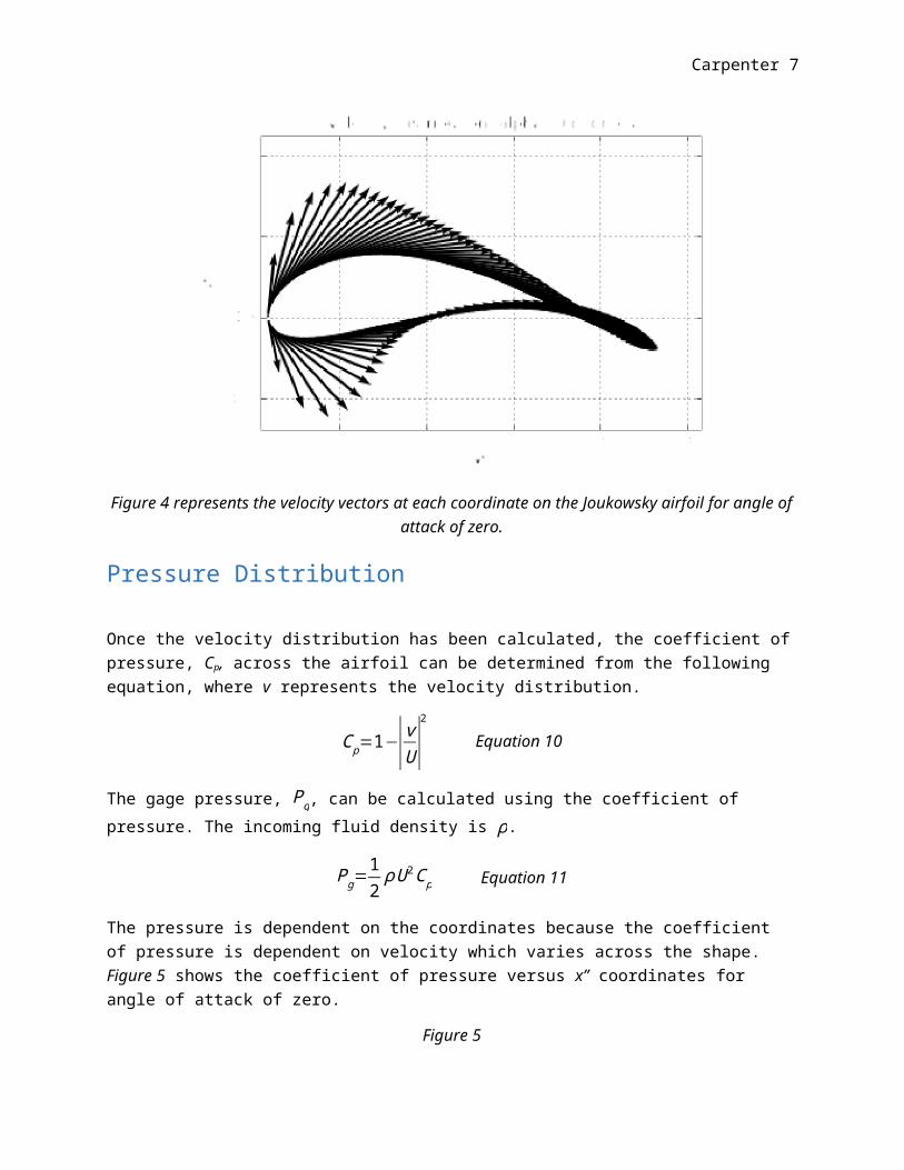
Figure 4 shows the velocity vector plot for the Joukowsky airfoil for an angle of attack of zero.

Figure 4

Figure 4 represents the velocity vectors at each coordinate on the Joukowsky airfoil for angle of attack of zero.

Pressure Distribution

Carpenter 6

Once the velocity distribution has been calculated, the coefficient of pressure, Cp, across the airfoil can be determined from the following equation, where v represents the velocity distribution.

C p=1−| vU |

2

Equation 10

The gage pressure, Pg, can be calculated using the coefficient of pressure. The incoming fluid density is ρ.

Pg=12

ρU 2C p Equation 11

The pressure is dependent on the coordinates because the coefficient of pressure is dependent on velocity which varies across the shape. Figure 5 shows the coefficient of pressure versus x” coordinates for angle of attack of zero.

Figure 5

Figure 5 presents the coefficient of pressure at angle of attack of zero. The plot reveals a lower pressure on the top of the airfoil and a higher pressure on the bottom of the airfoil.

Force Distribution

The pressure distribution can be utilized to find the force distribution. The force is the gage pressure acting on the area, A, of the airfoil.

F=A Pg Equation 12

The differential force is calculated for elements of the airfoil surface by multiplying the average pressure applied to the element by the distance it’s applied over, assuming the spanwise thickness in the z-direction is one.

Carpenter 7

dF ix=Pgi+Pg(i+1)

2( y i

} - {y} rsub {i+1} rsup { ) Equation 13

dF iy=Pgi+Pg (i+1)

2(x i +1

} - {x} rsub {i} rsup {) Equation 14

The total x-force, F x, and y-force, F y, are simply the sum of the elements of dF ix and dF iy.

F x=∑ dFix Equation 15

F y=∑ dF iy Equation 16

Coefficient of Lift

To evaluate the coefficient of lift, the airfoil’s lift force, L, must first be determined. This is the force perpendicular to the incoming freestream velocity.

L=−F x sinα+F y sin ( π2−α ) Equation 17

Finally the coefficient of lift, CL, can be calculated as follows, where c is the chordlength.

CL=L

12

ρU 2 c Equation 18

Results

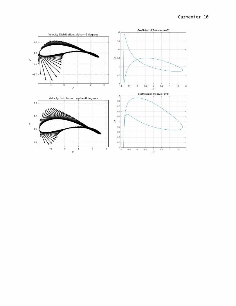
Figure 6 shows the velocity distribution and the coefficient of pressure for α=-10, -5, 0, 5, 10.

Figure 6

Carpenter 8

Carpenter 9

Figure 6 presents the velocity distribution and the coefficient of pressure versus x” for various angles of attack.

In the velocity plot for zero angle of attack the velocity is split around the leading edge at y ”=0. For the two negative angles of attack (-5⁰, -10⁰) the flow is split slightly above y ”=0, while for the two positive angles of attack (5⁰, 10⁰) it is split slightly below y ”=0. After the split the fluid flows tangential to the airfoil shape. For the larger magnitude of angles of attack there are larger vectors at the leading edge. In the 10⁰ angle of attack vector plot the vectors are very closely attached to the bottom surface, showing the fluid pushing against the bottom surface. On the top surface the fluid is going away from the surface on the leading edge end. This indicates a reduction of pressure on the top surface. With the vectors pushing against the surface on the bottom and moving away from the surface on the top, the lift phenomena is present.

In the pressure plots there is a low pressure on the top of the airfoil and a higher pressure on the bottom of the airfoil. Going from 5⁰ to 10⁰ the pressure difference increases. The plots with negative angle of attacks have an interesting pattern where the top surface and bottom surface pressures intersect so that toward the trailing edge the top surface has a higher pressure instead of lower. At 0⁰ angle of attack the pressure difference is the smallest.

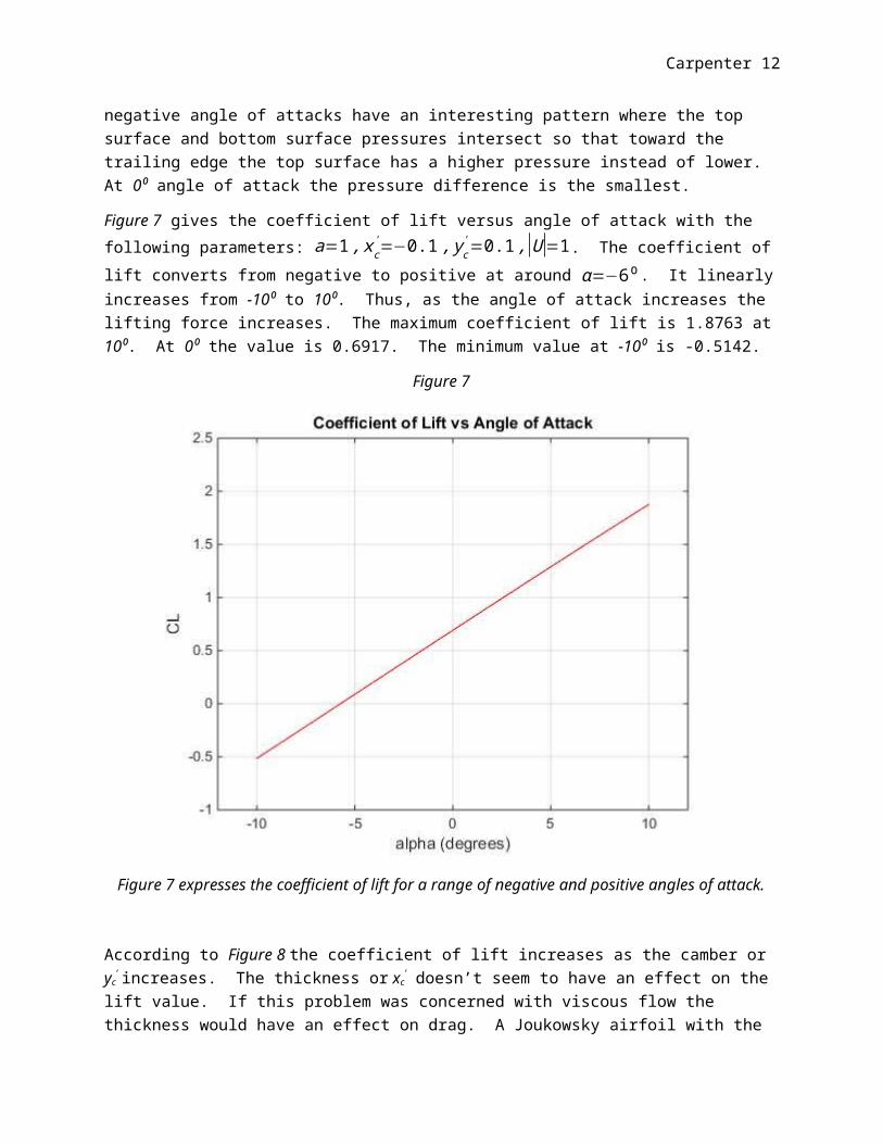
Figure 7 gives the coefficient of lift versus angle of attack with the following parameters: a=1 , xc

' =−0.1, yc' =0.1 ,|U|=1. The coefficient of lift converts from negative to positive at around

α=−6⁰. It linearly increases from -10⁰ to 10⁰. Thus, as the angle of attack increases the lifting force

Carpenter 10

increases. The maximum coefficient of lift is 1.8763 at 10⁰. At 0⁰ the value is 0.6917. The minimum value at -10⁰ is -0.5142.

Figure 7

Figure 7 expresses the coefficient of lift for a range of negative and positive angles of attack.

According to Figure 8 the coefficient of lift increases as the camber or yc’ increases. The thickness or xc

’ doesn’t seem to have an effect on the lift value. If this problem was concerned with viscous flow the thickness would have an effect on drag. A Joukowsky airfoil with the following parameters has a higher lift coefficient than the original plotted Joukowsky airfoil: a=1 , xc

' =−0.3 , yc' =0.5 ,|U|=1. This airfoil

is plotted in Figure 9.

Carpenter 11

Figure 8

Carpenter 12

Figure 8 shows plots of the coefficient of lift versus the angle of attack for various xc’ and yc

’ values.

Figure 9

In Figure 9 the Joukowsky airfoil is optimized by changing the xc' from -0.1 to 0.3 and the yc

' from 0.1 to 0.5. This magnified the camber to increase lift and enlarged the thickness to increase structural support.

Carpenter 13

This new airfoil design has an increased camber and thickness compared to the Joukowsky airfoil in Figure 3.4.3 of Advance Fluid Mechanics by W.P. Graebel. The new airfoil provides more lift as seen in Figure 10.

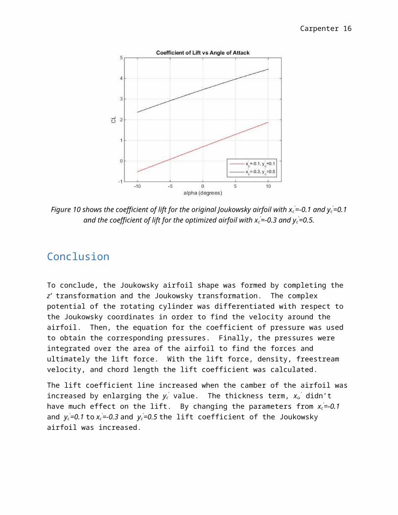
Figure 10

Figure 10 shows the coefficient of lift for the original Joukowsky airfoil with xc’=-0.1 and yc

’=0.1 and the coefficient of lift for the optimized airfoil with xc

’=-0.3 and yc’=0.5.

Conclusion

To conclude, the Joukowsky airfoil shape was formed by completing the z’ transformation and the Joukowsky transformation. The complex potential of the rotating cylinder was differentiated with respect to the Joukowsky coordinates in order to find the velocity around the airfoil. Then, the equation for the coefficient of pressure was used to obtain the corresponding pressures. Finally, the pressures were integrated over the area of the airfoil to find the forces and ultimately the lift force. With the lift force, density, freestream velocity, and chord length the lift coefficient was calculated.

The lift coefficient line increased when the camber of the airfoil was increased by enlarging the yc’ value.

The thickness term, xc,’ didn’t have much effect on the lift. By changing the parameters from xc’=-0.1 and

yc’=0.1 to xc

’=-0.3 and yc’=0.5 the lift coefficient of the Joukowsky airfoil was increased.

Carpenter 14

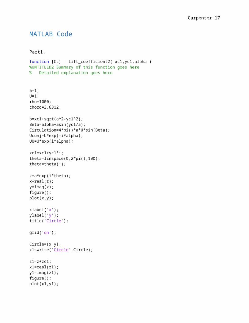
MATLAB Code

Part1.

function [CL] = lift_coefficient2( xc1,yc1,alpha )%UNTITLED2 Summary of this function goes here% Detailed explanation goes here a=1;U=1;rho=1000;chord=3.6312; b=xc1+sqrt(a^2-yc1^2);Beta=alpha+asin(yc1/a);Circulation=4*pi()*a*U*sin(Beta);Uconj=U*exp(-i*alpha);UU=U*exp(i*alpha); zc1=xc1+yc1*i;theta=linspace(0,2*pi(),100);theta=theta(:); z=a*exp(i*theta);x=real(z);y=imag(z);figure();plot(x,y); xlabel('x');ylabel('y');title('Circle'); grid('on'); Circle=[x y];xlswrite('Circle',Circle); z1=z+zc1;x1=real(z1);y1=imag(z1);figure();plot(x1,y1); xlabel('x1');ylabel('y1');title('Circle with Center (xc1,yc1)'); grid('on'); Circle2=[x1 y1];xlswrite('Circle2',Circle2);

Carpenter 15

z2=z1+(b^2./z1);x2=real(z2);y2=imag(z2);figure(); plot(x2,y2);axis([-2,2,-1,2]); xlabel('x"');ylabel('y"');title('Optimal Joukowsky Airfoil Shape'); grid('on'); Joukowsky=[x2 y2];xlswrite('Joukowsky2',Joukowsky); dwdz=Uconj-(UU./z.^2)+((i*Circulation)./(2*pi()*z));dwdz2=dwdz.*(z1.^2./(z1.^2-b^2)); vx=real(dwdz2);vy=-imag(dwdz2); v=[x2 y2 vx vy]; xlswrite('vectorplot',v); v2=sqrt(vx.^2+vy.^2); Cp=(1-(abs(v2/U)).^2);figure();plot(x2,Cp); xlabel('x2');ylabel('Cp');title('Coefficient of Pressure'); grid('on'); PP=.5*rho*UU^2*Cp;figure();plot(x2,PP); xlabel('x2');ylabel('PP');title('Pressure Distribution'); grid('on');

Carpenter 16

for g=1:99; dFiy=((PP(g,1)+PP(g+1,1))/2).*(x2(g+1,1)-x2(g,1)); dFix=((PP(g,1)+PP(g+1,1))/2).*(y2(g,1)-y2(g+1,1)); dFy(g,1)=dFiy; dFx(g,1)=dFix;end Fy=sum(dFy);Fx=sum(dFx); L=-Fx*sin(alpha)+Fy*sin((pi()/2)-alpha);CL=L/(.5*rho*UU^2*chord) end

Part2.

alphad=linspace(-10,10,21)alpha=alphad*2*pi()/360alpha=alpha(:)liftcoeffs=zeros(21,1) for k=1:21 al=alpha(k,1); coeff=lift_coefficient2(-0.1,0.1,al) liftcoeffs(k,1)=coeffend plot(alphad,liftcoeffs,'r') xlabel('alpha (degrees)')ylabel('CL')title('Coefficient of Lift vs Angle of Attack')grid('on')axis([-12,12,-1,2.5])

Part3.

alphad=linspace(-10,10,21)alpha=alphad*2*pi()/360alpha=alpha(:)liftcoeffs=zeros(21,1) for k=1:21 al=alpha(k,1); coeff=lift_coefficient2(-0.1,0.1,al) liftcoeffs(k,1)=coeff

Carpenter 17

end a1=plot(alphad,liftcoeffs,'r'); M1='x_c^''=-0.1, y_c^''=0.1' xlabel('alpha (degrees)')ylabel('CL')title('Coefficient of Lift vs Angle of Attack')grid('on')axis([-12,12,-1,5])hold on for k=1:21 al=alpha(k,1); coeff=lift_coefficient2(-0.3,0.5,al) liftcoeffs(k,1)=coeffend a2=plot(alphad,liftcoeffs,'k'); M2='x_c^''=-0.3, y_c^''=0.5' legend([a1; a2], [M1; M2],'Location','SouthEast');