Joseph F. HennawiUC Berkeley

&

OSUOctober 3, 2007

Xavier Prochaska(UCSC)

Quasars Probing QuasarsQuasars Probing QuasarsQuasars Probing QuasarsQuasars Probing Quasars

A Simple ObservationA Simple Observation

Spectrum from Wallace Sargent

The Basic PictureThe Basic Picture

HI cloud

Line-of-Sight

QSO

Transverse

b/g QSO

f/g QSOR||

R

HI cloud

• Ly absorption can probe 8 decades in NHI (Ly is large!).

• Neighboring sightline provides a another view of the QSO.

• Redshift space distortions from kT motions (~ 20 km/s ) smooth with Gaussian of Rprop ~ 60 kpc = 10” @ z = 2.

• Need projected QSO pairs to study small scales!

What Can Proximity Effects Teach Us?

What Can Proximity Effects Teach Us?

• How is HI distributed around quasars?

• What is the quasar duty cycle tQSO/tH ?• What is the obscured fraction (1- Ω/4)?

• Can we constrain episodic QSO variability, tburst?

• Directly observe impact of AGN feedback on the IGM?

nQSO(> L) :

tQSO

tH

Ω4

⎛⎝⎜

⎞⎠⎟nHost/Relics(> ?) ;

Ω4π

=nQSO

nQSO + nobscured

Physics of IGM well understood no sub-grid physics or semi-analytical recipes!

Mining Large SurveysMining Large SurveysApache Point Observatory (APO) • Spectroscopic QSO survey

– 5000 deg2

– 45,000 z < 2.2; i < 19.1– 5,000 z > 3; i < 20.2– Precise (u,g,r, i, z) photometry

• Photometric QSO sample– 8000 deg2

– 500,000 z < 3; i < 21.0– 20,000 z > 3; i < 21.0 – Richards et al. 2004; Hennawi et al. 2006

SDSS 2.5m

ARC 3.5m

Jim Gunn

Follow up QSO pair confirmation

from ARC 3.5m and MMT 6.5m

MMT 6.5m

= 3.7”

2’55”

ExcludedArea

Finding Quasar PairsFinding Quasar Pairs

SDSS QSO @ z =3.13

4.02.0

3.0

2.03.0

3.0

2.04.0

low-zQSOs

f/g QSO z = 2.29

b/g QSO z = 3.13

Keck LRIS spectra (Å)

Cosmology with Quasar PairsCosmology with Quasar PairsClose Quasar Pair Survey

• Discovered > 100 sub-Mpc pairs (z > 2) • Factor 25 increase in number known• Moderate & Echelle Resolution Spectra• Near-IR Foreground QSO Redshifts• About 50 Keck & Gemni nights.

= 13.8”, z = 3.00; Beam =79 kpc/h

Spectra from Keck ESI

Keck Gemini-N

Science• Dark energy at z > 2 from AP test

• Small scale structure of Ly forest

• Thermal history of the Universe

• Topology of metal enrichment from

• Transverse proximity effects

Gemini-S

Collaborators: Jason Prochaska, Crystal Martin, Sara Ellison, George Djorgovski, Scott Burles

Ly Forest Correlations

CIV Metal Line Correlations

Nor

mal

ized

Flu

x

Quasar Absorption LinesQuasar Absorption Lines

DLA (HST/STIS)

Moller et al. (2003)

LLS

Nobody et al. (200?)

Lyz = 2.96

Lyman Limitz = 2.96

QSO z = 3.0 LLS

Lyz = 2.58

DLA

• Ly Forest– Optically thin diffuse IGM / ~ 1-10; 1014 < NHI < 1017.2

– well studied for R > 1 Mpc/h

• Lyman Limit Systems (LLSs)– Optically thick 912 > 1

– 1017.2 < NHI < 1020.3

– almost totally unexplored

• Damped Ly Systems (DLAs)– NHI > 1020.3 comparable to disks

– sub-L galaxies?

– Dominate HI content of Universe

Self Shielding: A Local ExampleSelf Shielding: A Local Example

Sharp edges of galaxy disks set by ionization equilibrium with the UV background. HI is ‘self-shielded’ from extragalactic UV photons.

Braun & Thilker (2004)M31 (Andromeda) M33 VLA 21cm map

DLA

Ly forest

LLS

What if the MBH = 3107 M black hole at Andromeda’s center started accreting at the Eddington limit? What would M33 look like then?

bump due

to M33

Average HI of Andromeda

Neutral Gas

Isolated QSO

Proximity EffectsProximity Effects

• Proximity Effect Decrease in Ly forest absorption due to large ionizing flux near a quasar

• Transverse Proximity Effect Decrease in absorption in background QSO spectrum due to transverse ionizing flux of a foreground quasar– Geometry of quasar radiation field (obscuration?)

– Quasar lifetime/variability

– Measure distribution of HI in quasar environments

Are there similar effects for optically thick absorbers?

Ionized Gas

Projected QSO Pair

nQSO :

tQSO

tH

Ω4

⎛⎝⎜

⎞⎠⎟nHosts

Transverse Optically ThickTransverse Optically Thick

Hennawi, Prochaska, et al. (2007)

zbg = 3.13; zfg= 2.29; R = 22 kpc/h; logNHI = 20.5

zbg = 2.07; zfg= 1.98; R = 139 kpc/h; logNHI = 19.0

zbg = 2.21; zfg= 2.18; R = 61 kpc/h; logNHI = 18.5

zbg = 2.53; zfg= 2.43; R = 78 kpc/h; logNHI = 19.7

zbg = 2.35; zfg= 2.28; R = 37 kpc/h; logNHI = 18.9

zbg = 2.17; zfg= 2.11; R = 97 kpc/h; logNHI = 20.3

Transverse Optically Thick Clustering

Transverse Optically Thick ClusteringHennawi, Prochaska et al. (2007);

Hennawi & Prochaska (2007)

= Keck = Gemini = SDSS

= has absorber = no absorber

En

han

cem

ent

over

UV

Bz

(re

dsh

ift)

= 2.0 = 1.6

QSO-LBG

• 29 new QSO-LLSs with R < 2 Mpc/h

• High covering factor for R < 100 kpc/h

• For T(r) = (r/rT)-, = 1.6, log NHI > 19

rT = 9 1.7 Mpc/h (3 QSO-LBG)

Line-of-Sight ClusteringLine-of-Sight Clustering

Prochaska, Hennawi, & Herbert-Fort (2007)

• Factor 5-10 fewer PDLAs then expected from transverse clustering.

• Transverse clustering strength at z = 2.5 predicts that ~ 90% of QSO’s should

have an absorber with NHI > 1019 cm-2 along the LOS??

• Rapid redshift evolution of QSO clustering compared to paucity of proximate

DLAs implies that photoevaporation has to be occurring.

Transverse prediction

1 +

||(

∆v)

z

Line-of-Sight Clustering Strength

Extrapolation of trans. predictions

Line-of-sight measurements

Proximate DLA DLA within v < 3000 km/s

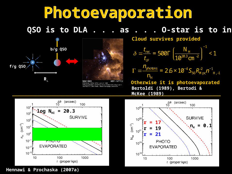
PhotoevaporationPhotoevaporation

f/g QSO

b/g QSO

R

QSO is to DLA . . . as . . . O-star is to interstellar cloud

Γ =nphotons

nH

= 2.6 ×10−4S56RMpc-2 n−1

H, -1

Hennawi & Prochaska (2007a)

δ =trect IF

= 500ΓNH

1020.3cm-2

⎛⎝⎜

⎞⎠⎟

−1

< 1

Otherwise it is photoevaporatedBertoldi (1989), Bertodi & McKee (1989)

Cloud survives provided

r = 17r = 19r = 21

nH = 0.1

log NHI = 20.3

Emission AnisotropyEmission AnisotropyObscuration/Beaming

f/g QSO

b/g QSO

Absorber

R

Ω > 104 yr

• Episodic Variability QSO’s vary significantly on timescale

t < tcross ~ 4 105 yr @ = 20” (120 kpc/h).

Current best limit is tburst > 104 yr.

Episodic Variability

f/g QSO

b/g QSO

Absorber

We observe light emitted at time t = t0

Ionization state of gas depends on QSO at time t = t0 - R/c R

t = t0

• Optically Thick LLSs and DLAs (today’s talk)

– Nature of absorbers near QSO’s is unclear.

• Gas entrained from AGN driven outflow? (AGN feedback!)

• Absorption from nearby dwarf galaxies?

– To measure tQSO/tH or (Ω/4) we need to model

absorbers and do radiative transfer (hard).

• Optically Thin Ly Forest (in progess)

– Best for constraining tQSO/tH and (Ω/4).

– Why? Because we can predict the Ly forest

fluctuations ab initio from N-body simulations (easy).

Proximity Effects: Thick and ThinProximity Effects: Thick and Thin

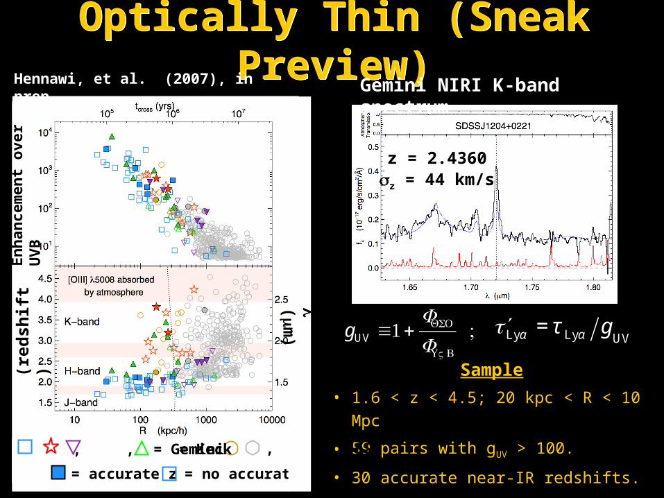
Optically Thin (Sneak Preview)Optically Thin (Sneak Preview)Hennawi, et al. (2007), in prep

= Gemini

= accurate z = no accurate z

En

han

cem

ent

over

UV

Bz

(re

dsh

ift)

Sample

• 1.6 < z < 4.5; 20 kpc < R < 10 Mpc

• 59 pairs with gUV > 100.

• 30 accurate near-IR redshifts.

(

m)

, , = Keck , = SDSS

gUV ≡1+FQSO

FUVB

; ′Lyα = τ Lyα gUV

z = 2.4360z = 44 km/s

Gemini NIRI K-band spectrum

Transverse Proximity Effect?Transverse Proximity Effect?

z = 3.8135

z = 44 km/s

zbg = 4.11, zfg= 3.81

= 34”, R = 175 kpc/h

tcross = 5.7107 yr

gUV = 626!

with f/g QSO

without f/g QSO

RealReal

SimulatedSimulated

Hennawi et al. 2007, in prep.

Gemini NIRI K-band spectrumSpectrum from Keck ESI

SummarySummary• With projected pairs, QSO environments can be probed

down to ~ 20 kpc where ionizing flux is ~ 104 times the UVB.

• Clustering of optically thick absorbers around QSOs is highly anisotropic.

• Paucity of PDLAs implies photoevaporation has to occur.

• Physical arguments indicate DLAs < 1 Mpc from a QSO can

be photoevaporated.

• There is a LOS optically thick proximity effect but no transverse one.

• Either QSOs emit anisotropically or are variable on timescales < 106 yr.

• The optically thin proximity effect will distinguish between these two possibility and yield new quantitative constraints.