Joint Learning from Earth Observation and OpenStreetMap Data

to Get Faster Better Semantic Maps

Nicolas Audebert, Bertrand Le Saux

ONERA, The French Aerospace Lab

F-91761 Palaiseau, France

(nicolas.audebert,bertrand.le_saux)@onera.fr

Sébastien Lefèvre

Univ. Bretagne-Sud, UMR 6074, IRISA

F-56000 Vannes, France

sebastien.lefevre@irisa.fr

Abstract

In this work, we investigate the use of OpenStreetMap

data for semantic labeling of Earth Observation images.

Deep neural networks have been used in the past for re-

mote sensing data classification from various sensors, in-

cluding multispectral, hyperspectral, SAR and LiDAR data.

While OpenStreetMap has already been used as ground

truth data for training such networks, this abundant data

source remains rarely exploited as an input information

layer. In this paper, we study different use cases and deep

network architectures to leverage OpenStreetMap data for

semantic labeling of aerial and satellite images. Espe-

cially, we look into fusion based architectures and coarse-

to-fine segmentation to include the OpenStreetMap layer

into multispectral-based deep fully convolutional networks.

We illustrate how these methods can be successfully used

on two public datasets: ISPRS Potsdam and DFC2017. We

show that OpenStreetMap data can efficiently be integrated

into the vision-based deep learning models and that it sig-

nificantly improves both the accuracy performance and the

convergence speed of the networks.

1. Introduction

Dense labeling of remote sensing data is a common task

to generate semantic maps of large areas automatically, ei-

ther to perform cartography of urban areas or to determine

land use covers at a large scale. Many techniques that orig-

inated in the computer vision community for semantic seg-

mentation can be applied on Red-Green-Blue (RGB) re-

mote sensing data to this end and has been successfully used

with state-of-the-art results, e.g. Convolutional Neural Net-

works (CNN) for land use classification [4] or Fully Con-

volutional Networks (FCN) for semantic labeling of urban

areas [1]. Yet, remote sensing data is rarely limited to RGB

channels. Often, multiple sensors are used to obtain com-

plementary physical information about the observed area,

with the final products being co-registered multispectral,

LiDAR and SAR data. Several works successfully inves-

tigated semantic labeling of remote sensing data using fu-

sion of multiple heterogeneous sensors [1, 26, 16] to lever-

age complementary informations sources. However, there

is still a huge untapped source of information: the public

geo-information system (GIS) databases that rely on volun-

tary crowdsourced annotations. These databases, such as

the very popular OpenStreetMap (OSM), are an extremely

valuable source of information, that is mostly used as a

training ground truth [24] as it contains data layers such as

roads, buildings footprints or forest coverage. But this data

can also be seen as an alternative input layer that will pro-

vide another information channel compared to the classical

sensors. Consequently, we investigate here the following

question: how can we use OSM data to improve sensor-

based semantic labeling of remote sensing data ?

2. Related work

Semantic labeling of aerial and satellite images using

deep neural networks has been investigated several times

in the literature. Since the early work on road extraction

using CNN [24], many studies investigated deep neural net-

works for automatic processing of aerial and satellite data.

The most recent works using deep learning mostly focus

on the use of Fully Convolutional Networks [20], an ar-

chitecture initially designed for semantic segmentation of

multimedia images, and later successfully applied to re-

mote sensing data at various resolutions. This type of

deep models obtained excellent results on very high reso-

lution datasets [28], often combined with multiscale anal-

ysis [1], graphical model post-processing [33] and bound-

ary prediction [22]. The same architectures were also suc-

cessful for building and roads extraction from satellite im-

ages [21, 31, 34] at a significantly lower resolution.

Although most of the works are limited to optical data,

e.g. RGB or multispectral images, the fusion of hetero-

geneous data layers has also been investigated in several

67

works. Notably, multimodal processing of very high resolu-

tion images has been successfully applied to a combination

of deep features and superpixel classification in [3], while

a deep framework for the fusion of video and multispectral

data was proposed in [25]. Fusion of multitemporal data for

joint registration and change detection was investigated in

[32]. Heterogeneous data fusion was also explored through

deep features mixed with hand-crafted features for random

forest classification [26], and later using end-to-end deep

networks in [1] for LiDAR and RGB data, and [16] for hy-

perspectral and SAR data.

While all these works investigated data fusion of var-

ious sensors, they did not study the inclusion of highly

processed, semantically richer data such as OpenStreetMap

layers. Indeed, since the launch of OpenStreetMap (OSM)

and Google Maps in 2004, map data became widely avail-

able and have been largely used within remote sensing

applications. First, they can be used as targets for deep

learning algorithms, such as in the seminal work of Mnih

[24, 23], since those layers already provide accurate in-

formation about the buildings and roads footprints. More

recent works in simultaneous registration and classifica-

tion [32] and large-scale classification [21, 6] also rely on

OSM data to perform supervised learning. The generation

of OpenStreetMap rasters from optical images with Gener-

ative Adversarial Networks has also been investigated [17],

but the authors did not evaluate their method with classifi-

cation metrics as they were only interested by perceptually

coherent image-to-image translation. Second, the map lay-

ers can be used as inputs of a processing flow to produce

new geo-spatial data. Although the coverage and the qual-

ity of the annotations from open GIS vary a lot depending

on the users’ knowledge and number of contributors, this

data may contain relevant information for mapping specific

areas and classes. A deterministic framework to create land

use and land cover maps from crowdsourced maps such as

OSM data was proposed in [10]. Machine learning tools (a

random forest variant) also allow coupling remote sensing

and volunteered geographic information (VGI) to predict

natural hazard exposure [11] and local climate zones [8],

while active deep learning helps finding unlabeled objects

in OSM [5]. However, to the best of our knowledge, no

VGI has been used as an input (opposite of a target) in deep

neural networks yet.

3. Method

In this work, we investigate two use cases for highly

structured semantic data as input to deep networks. The first

one occurs when the semantic data is close to the ground

truth, in our case where OpenStreetMap already contains a

part of the information we want to label, e.g. finding roads

in airborne images. The second one occurs when what we

want to label can be inferred from OpenStreetMap but only

indirectly, for example when we want to derive the type of

settlement based on building footprints.

3.1. Coarse­to­fine segmentation

In some cases, OpenStreetMap data can be used as a

coarse approximation from the ground truth, e.g. for objects

such as buildings and roads. Therefore, we would need only

to learn how to refine this coarse map to obtain the final very

high resolution pixel-wise segmentation. Especially, learn-

ing only this difference can be seen as a form of residual

learning [15] which should help the training process. This

was also suggested in [19] to help the classification process

by first learning coarse approximations of the ground truth

before iteratively refining the predictions.

In our case, we can use a simple FCN with only two lay-

ers to convert the raw rasterized OSM data into a semantic

map that approximates the ground truth, trained with the

usual backpropagation technique. This FCN will be de-

noted OSMNet in the following sections. OSMNet only

manipulates the original OSM map to project it in a rep-

resentation space compatible with the ground truth classes.

The optical data will then be used as input to a FCN model

to infer a semantic segmentation that will complete the ap-

proximate map derived from OSM. In this work, we will

use the SegNet architecture [2] that we will train following

the guidelines from [1]. SegNet is an encoder-decoder deep

neural network that projects an input image into a seman-

tic map with the same resolution. Using these two models,

we can compute the average prediction computed using the

two data sources. In this framework, if we denote I the

input image, O the input OSM raster, Popt the prediction

function for SegNet and Posm the prediction function for

OSMNet, the final prediction P is:

P (I,O) =1

2(Popt(I) + Posm(O)) . (1)

If Posm(O) is already an adequate approximation of the

ground truth GT , then the training process will try to mini-

mize:

Popt ∝ GT − Posm(O) ≪ GT , (2)

which should have a similar effect on the training process

than the residual learning from [15].

Moreover, to refine even further this average map, we use

a residual correction network [1]. This module consists in a

residual three-layer FCN that learns how to correct the av-

erage prediction using the complementary information from

the OSM and optical data sources. If we denote C the pre-

diction function of the residual correction network, we fi-

nally have:

P (I,O) =1

2(Popt(I)+Posm(O))+C(Zopt(I), Zosm(O)) ,

(3)

68

RGB

OSM

CNNconv + BN + ReLU

densepredictions

densepredictions

concat

fusion

densepredictions

softm

ax

⊕

⊕

Encoderconv + BN + ReLU

+ pooling

Decoderupsampling +

conv + BN + ReLU

Segmentation

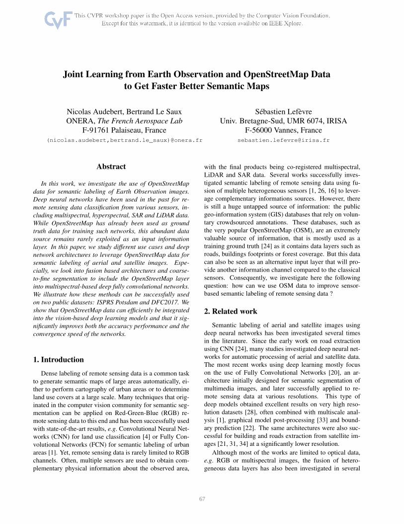
(a) Optical and OSM data fusion using residual correction [1].

RGB

OSM ⊕ ⊕ ⊕ ⊕ ⊕

densepredictions

softm

ax

Encoderconv + BN + ReLU + pooling

Decoderupsampling + conv + BN + ReLU

Segmentation

(b) FuseNet [13] architecture applied to optical and OSM data.

Figure 1: Deep learning architectures for joint processing of optical and OpenStreetMap data.

where Zopt and Zosm are the last feature maps from SegNet

and OSMNet, respectively.

The residual learning using this module can be seen as

learning an error correction to refine and correct occasional

errors in the prediction. The full pipeline is illustrated in

the Fig. 1a. The whole architecture is trained jointly.

3.2. Dual­stream convolutional neural networks

FCN with several sources have been investigated several

times in the past, notably for processing RGB-D (or 2.5D)

images in the computer vision community [9]. In this work,

we use the FuseNet architecture [13] to combine optical and

OSM data. It is based on the popular SegNet [2] model.

FuseNet has two encoders, one for each source. After each

convolutional block, the activations maps from the second

encoder are summed into the activations maps from the first

encoder. This allows the two encoders to learn a joint repre-

sentation of the two modalities. Then, a single decoder per-

forms both the spatial upsampling and the pixel-wise clas-

sification. As detailed in Fig. 1b, one main branch learns

this joint summed representation while the ancillary branch

learns only OSM-dependent activations. If we denote P the

prediction function from FuseNet, I the input image, O the

input OSM rasters, E{opt,osm}i the encoded feature maps

after the ith block, B{opt,osm}i the encoding functions for

the ith block and D the decoding function:

P (I,O) = D(Eopt5 (I,O)) (4)

and

Eopti+1

(I,O) = Bopti (Eopt

i (I,O))+Bosmi (Eosm

i (O)) . (5)

This architecture allows us to fuse both data streams in the

internal representation learnt by the network. This model is

illustrated in Fig. 1b.

4. Experiments

4.1. Datasets

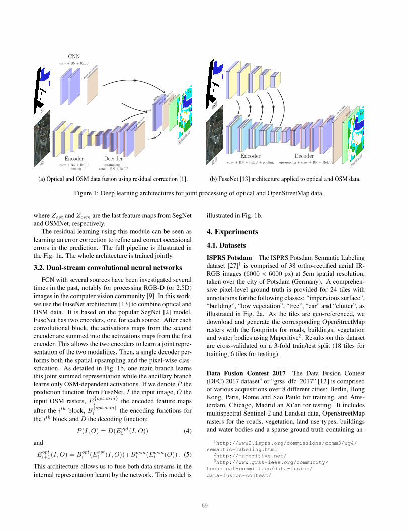
ISPRS Potsdam The ISPRS Potsdam Semantic Labeling

dataset [27]1 is comprised of 38 ortho-rectified aerial IR-

RGB images (6000 × 6000 px) at 5cm spatial resolution,

taken over the city of Potsdam (Germany). A comprehen-

sive pixel-level ground truth is provided for 24 tiles with

annotations for the following classes: “impervious surface”,

“building”, “low vegetation”, “tree”, “car” and “clutter”, as

illustrated in Fig. 2a. As the tiles are geo-referenced, we

download and generate the corresponding OpenStreetMap

rasters with the footprints for roads, buildings, vegetation

and water bodies using Maperitive2. Results on this dataset

are cross-validated on a 3-fold train/test split (18 tiles for

training, 6 tiles for testing).

Data Fusion Contest 2017 The Data Fusion Contest

(DFC) 2017 dataset3 or “grss_dfc_2017” [12] is comprised

of various acquisitions over 8 different cities: Berlin, Hong

Kong, Paris, Rome and Sao Paulo for training, and Ams-

terdam, Chicago, Madrid an Xi’an for testing. It includes

multispectral Sentinel-2 and Landsat data, OpenStreetMap

rasters for the roads, vegetation, land use types, buildings

and water bodies and a sparse ground truth containing an-

1http://www2.isprs.org/commissions/comm3/wg4/

semantic-labeling.html2http://maperitive.net/3http://www.grss-ieee.org/community/

technical-committees/data-fusion/

data-fusion-contest/

69

Potsdam (RGB) Potsdam (GT)

(a) ISPRS Potsdam dataset

DFC 2017 (false RGB) DFC 2017 (GT)

(b) DFC 2017 dataset (extract from São Paulo)

Figure 2: Extract of the ISPRS Potsdam and DFC2017 datasets

notations for several Local Climate Zones (LCZ), as illus-

trated in Fig. 2b. The LCZ define urban or rural areas such

as “sparsely built urban area”, “water body”, “dense trees”

and so on, using the taxonomy from [30]. The annotations

cover only a part of the cities and are provided at 100m/pixel

resolution. The goal is to generalize those annotations to

the testing cities. In this work, we use the multispectral

20m/pixel resolution Sentinel-2 data and the OSM raster for

roads, buildings, vegetation and water bodies. We prepro-

cess the multispectral data by clipping the 2% highest val-

ues. All 13 bands are kept and stacked as input to the neural

network. As Sentinel-2 multispectral data includes bands

at 10m/pixel, 20m/pixel and 60m/pixel resolutions, bands

that have a resolution lower or higher than 20m/pixel are

rescaled using bilinear interpolation. Results on this dataset

are computed on the held-out testing set from the bench-

mark.

4.2. Experimental setup

We train our models on the ISPRS Potsdam dataset in an

end-to-end fashion, following the guidelines from [1]. We

randomly extract 128×128 patches from the RGB and OSM

training tiles on which we apply random flipping or mirror-

ing as data augmentation. The optimization is performed

with a batch size of 10 on the RGB tiles using a Stochas-

tic Gradient Descent (SGD) with a learning rate of 0.01

divided by 10 every 2 epochs (≃ 30 000 iterations). Seg-

Net’s encoder for the RGB data is initialized using VGG-

16 [29] weights trained on ImageNet, while the decoder

is randomly initialized using the MSRA [14] scheme. The

learning rate for the encoder is set to half the learning rate

for the decoder. During testing, each tile is processed by

sliding a 128 × 128 window with a stride of 64 (i.e. 50%

overlap). Multiple predictions for overlapping regions are

averaged to smooth the map and reduce visible stitching on

the patch borders. Training until convergence (≃ 150,000

iterations) takes around 20 hours on a NVIDIA K20c, while

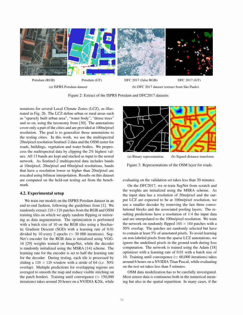
(a) Binary representation. (b) Signed distance transform.

Figure 3: Representations of the OSM layer for roads.

evaluating on the validation set takes less than 30 minutes.

On the DFC2017, we re-train SegNet from scratch and

the weights are initialized using the MSRA scheme. As

the input data has a resolution of 20m/pixel and the out-

put LCZ are expected to be at 100m/pixel resolution, we

use a smaller decoder by removing the last three convo-

lutional blocks and the associated pooling layers. The re-

sulting predictions have a resolution of 1:4 the input data

and are interpolated to the 100m/pixel resolution. We train

the network on randomly flipped 160 × 160 patches with a

50% overlap. The patches are randomly selected but have

to contain at least 5% of annotated pixels. To avoid learning

on non-labeled pixels from the sparse LCZ annotations, we

ignore the undefined pixels in the ground truth during loss

computation. The network is trained using the Adam [18]

optimizer with a learning rate of 0.01 with a batch size of

10. Training until convergence (≃ 60,000 iterations) takes

around 6 hours on a NVIDIA Titan Pascal, while evaluating

on the test set takes less than 5 minutes.

OSM data modelization has to be carefully investigated.

Most sensor data is continuous both in the numerical mean-

ing but also in the spatial repartition. In many cases, if the

70

original data is not continuous but sparse, well-chosen rep-

resentations are used to get the continuity back, e.g. the Dig-

ital Surface Model which is a continuous topology extracted

from the sparse LiDAR point cloud. In our case, the OSM

data is sparse and discrete like the labels. Therefore, it is

dubious if the deep network will be able to handle all the

information using such a representation. We compare two

representations, illustrated in Fig. 3:

• Sparse tensor representation, which is discrete. For

each raster, we have an associated channel in the ten-

sor which is a binary map denoting the presence of the

raster class in the specified pixel (cf. Fig. 3a).

• Signed distance transform (SDT) representation,

which is continuous. We generate for each raster the

associated channel corresponding to the distance trans-

form d, with d > 0 if the pixel is inside the class and

d < 0 if not (cf. Fig. 3b, with a color range from blue

to red).

The signed distance transform was used in [34] for build-

ing extraction in remote sensing data. The continuous rep-

resentation helped densifying the sparse building footprints

that were extracted from a public GIS database and success-

fully improved the classification accuracy.

4.3. Results

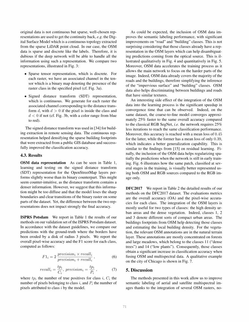
OSM data representation As can be seen in Table 1,

learning and testing on the signed distance transform

(SDT) representation for the OpenStreetMap layers per-

forms slightly worse than its binary counterpart. This might

seem counter-intuitive, as the distance transform contains a

denser information. However, we suggest that this informa-

tion might be too diffuse and that the model loses the sharp

boundaries and clear transitions of the binary raster on some

parts of the dataset. Yet, the difference between the two rep-

resentations does not impact strongly the final accuracy.

ISPRS Potsdam We report in Table 1 the results of our

methods on our validation set of the ISPRS Potsdam dataset.

In accordance with the dataset guidelines, we compare our

predictions with the ground-truth where the borders have

been eroded by a disk of radius 3 pixels. We report the

overall pixel-wise accuracy and the F1 score for each class,

computed as follows:

F1i = 2precisioni × recalli

precisioni + recalli, (6)

recalli =tpi

Ci

, precisioni =tpi

Pi

, (7)

where tpi the number of true positives for class i, Ci the

number of pixels belonging to class i, and Pi the number of

pixels attributed to class i by the model.

As could be expected, the inclusion of OSM data im-

proves the semantic labeling performance, with significant

improvements on “road” and “building” classes. This is not

surprising considering that those classes already have a rep-

resentation in the OSM layers which can help disambiguat-

ing predictions coming from the optical source. This is il-

lustrated qualitatively in Fig. 4 and quantitatively in Fig. 5.

Moreover, OSM data accelerates the training process as it

allows the main network to focus on the harder parts of the

image. Indeed, OSM data already covers the majority of the

roads and the buildings, therefore simplifying the inference

of the “impervious surface” and “building” classes. OSM

data also helps discriminating between buildings and roads

that have similar textures.

An interesting side effect of the integration of the OSM

data into the learning process is the significant speedup in

convergence time that can be observed. Indeed, on the

same dataset, the coarse-to-fine model converges approxi-

mately 25% faster to the same overall accuracy compared

to the classical RGB SegNet, i.e. the network requires 25%

less iterations to reach the same classification performance.

Moreover, this accuracy is reached with a mean loss of 0.45for the latter, while the former has a mean loss of only 0.39,

which indicates a better generalization capability. This is

similar to the findings from [15] on residual learning. Fi-

nally, the inclusion of the OSM data helps regularizing spa-

tially the predictions when the network is still in early train-

ing. Fig. 6 illustrates how the same patch, classified at sev-

eral stages in the training, is visually better represented us-

ing both OSM and RGB sources compared to the RGB im-

age only.

DFC2017 We report in Table 2 the detailed results of our

methods on the DFC2017 dataset. The evaluations metrics

are the overall accuracy (OA) and the pixel-wise accura-

cies for each class. The integration of the OSM layers is

mostly useful for two types of classes: the high density ur-

ban areas and the dense vegetation. Indeed, classes 1, 2

and 3 denote different sorts of compact urban areas. The

buildings footprints from OSM help detecting those classes

and estimating the local building density. For the vegeta-

tion, the relevant OSM annotations are in the natural terrain

layer. These annotations are mostly concentrated on forests

and large meadows, which belong to the classes 11 (“dense

trees”) and 14 (“low plants”). Consequently, those classes

obtain a significant increase in classification accuracy when

fusing OSM and multispectral data. A qualitative example

on the city of Chicago is shown in Fig. 7.

5. Discussion

The methods presented in this work allow us to improve

semantic labeling of aerial and satellite multispectral im-

ages thanks to the integration of several OSM rasters, no-

71

Table 1: Test results on the ISPRS Potsdam dataset (pixel-wise overall accuracy and F1 score per class).

OSM Method imp. surfaces buildings low veg. trees cars Overall

Binary OSMNet 54.8 90.0 51.5 0.0 0.0 60.3

∅ SegNet RGB 93.0 92.9 85.0 85.1 95.1 89.7

BinaryResidual Correction RGB+OSM 93.9 92.8 85.1 85.2 95.8 90.6

FuseNet RGB+OSM 95.3 95.9 86.3 85.1 96.8 92.3

SDTResidual Correction RGB+OSM 93.8 92.7 85.2 84.8 95.9 90.5

FuseNet RGB+OSM 95.2 95.9 86.4 85.0 96.5 92.3

Table 2: Test results on the DFC2017 dataset (pixel-wise accuracies)

LCZ

Urban Rural

Compact OpenMisc.

buildingsTrees Vegetation Soils and water

1 2 3 4 5 6 7 8 9 10 11 12 13 14 15 16 17 OA

SegNet multispectral 34.7 25.4 8.6 19.7 14.6 17.5 0.0 62.3 0.0 1.0 66.9 4.3 13.1 62.5 0.0 0.0 89.2 41.7

FuseNet multispectral + OSM 34.3 39.1 26.0 16.7 6.2 37.1 0.0 45.2 9.2 0.0 83.4 1.8 0.0 80.2 1.4 0.0 87.3 46.5

tably the roads, buildings and vegetation land use. However,

OpenStreetMap data is much more exhaustive than such

layers and also contains specific information (e.g. swamps,

agriculture fields, industrial areas, different categories of

roads. . . ). However, if all information are stacked by us-

ing one map per layer of interest, the OSM memory foot-

print would become huge very quickly, especially consider-

ing that OSM provides vector information that can be ras-

terized at any spatial resolution. In our case, we rasterize

the OSM layers to the same resolution as our input image,

which can be very high for airborne acquisitions. Moreover,

we have not addressed here the question of the subclassifi-

cation, while this is definitely a source of future improve-

ment. Indeed, thanks to OSM data, we can know that some

specific buildings have a particular type, e.g. a building can

be a church, a grocery store or a house. Point annotations,

such as parking lots, are also dismissed but could provide

meaningful insights about the semantics of the area. Fur-

thermore, we underline that even though the OSM layers

that we used were more recent (2 years) than to the optical

data, there were few enough disagreements so that the mod-

els were robust to those conflicts. Yet, data fusion should

be done carefully if the sources do not represent the same

underlying reality. In the case of the OSM data, this could

be worked around by extracting the layers from the OSM

archives if the optical data is not recent enough. Finally,

mapping style and coverage can vary a lot based on the

observed regions. For example, urban areas in developed

countries are thoroughly mapped, whereas annotations are

very scarce in rural areas in developing countries. This en-

forces the need for the model to be robust to errors and miss-

ing OSM input data for very large scale mapping.

6. Conclusion

In this work, we showed how to integrate ancillary GIS

data in deep learning-based semantic labeling. We pre-

sented two methods: one for coarse-to-fine segmentation,

using deep learning on RGB data to refine OpenStreetMap

semantic maps, and one for data fusion to merge multispec-

tral data and OSM rasters to predict local climate zones. We

validated our methods on two public datasets: the ISPRS

Potsdam 2D Semantic Labeling Challenge and the Data Fu-

sion Contest 2017. We increase our semantic labeling over-

all accuracy by 2.5% on the former and by nearly 5% on

the latter by integrating OpenStreetMap data in the learning

process. Moreover, on the ISPRS Potsdam dataset, using

OSM layers in a residual correction fashion accelerates the

model convergence by 25%. Our findings show that GIS

sparse data can be leveraged successfully for semantic la-

beling on those two use cases, as it improves significantly

the classification accuracy of the models. We think that us-

ing crowdsourced and open GIS data is an exciting topic

of research, and this work provides new insights on how to

use this data to improve and accelerate learning based on

traditional sensors.

Acknowledgements

The Vaihingen dataset was provided by the Ger-

man Society for Photogrammetry, Remote Sensing and

Geoinformation (DGPF) [7]: http://www.ifp.

uni-stuttgart.de/dgpf/DKEP-Allg.html.

72

(a) RGB input (b) OSM input (c) Target ground truth

(d) SegNet (RGB) (e) FuseNet (OSM+RGB)

Figure 4: Excerpt from the classification results on Potsdam

The authors thank the ISPRS for making the Vaihingen and

Potsdam datasets available and organizing the semantic

labeling challenge. The authors would like to thank

the WUDAPT (http://www.wudapt.org/) and

GeoWIKI (http://geo-wiki.org/) initiatives and

the IEEE GRSS Image Analysis and Data Fusion Technical

Committee. Nicolas Audebert’s work is supported by the

Total-ONERA research project NAOMI.

References

[1] N. Audebert, B. Le Saux, and S. Lefèvre. Semantic Seg-

mentation of Earth Observation Data Using Multimodal and

Multi-scale Deep Networks. In Computer Vision – ACCV

2016, pages 180–196. Springer, Cham, Nov. 2016.

[2] V. Badrinarayanan, A. Kendall, and R. Cipolla. SegNet:

A Deep Convolutional Encoder-Decoder Architecture for

Scene Segmentation. IEEE Transactions on Pattern Anal-

ysis and Machine Intelligence, PP(99):1–1, 2017.

[3] M. Campos-Taberner, A. Romero-Soriano, C. Gatta,

G. Camps-Valls, A. Lagrange, B. Le Saux, A. Beaupère,

A. Boulch, A. Chan-Hon-Tong, S. Herbin, H. Randrianarivo,

M. Ferecatu, M. Shimoni, G. Moser, and D. Tuia. Processing

of Extremely High-Resolution LiDAR and RGB Data: Out-

come of the 2015 IEEE GRSS Data Fusion Contest Part A: 2-

D Contest. IEEE Journal of Selected Topics in Applied Earth

Observations and Remote Sensing, PP(99):1–13, 2016.

73

impervious surfaces buildings low vegetation trees cars

cars

trees

low vegetation

buildings

impervious surfaces

49485 14444 1754 35150 3010013

521341 57615 3122028 19490186 44788

1108857 558643 35856853 2083046 352

1664120 51520875 2967059 111546 76285

62297705 1126605 1878448 725054 21838

1.5

3.0

4.5

6.0

1e7

(a) SegNet RGB

impervious surfaces buildings low vegetation trees cars

cars

trees

low vegetation

buildings

impervious surfaces

57425 18174 665 39127 2999795

561322 66035 3004559 19578633 39992

1485836 485991 35536974 2206183 658

1316018 52340387 2541862 112340 90877

62840673 906387 1553010 697701 28881

1.5

3.0

4.5

6.0

1e7

(b) Residual Correction OSM+RGB

impervious surfaces buildings low vegetation trees cars

cars

trees

low vegetation

buildings

impervious surfaces

48348 25658 2871 37085 3001551

474568 49960 2658349 20038376 44156

1218568 583730 35235082 2715956 213

2549169 50056828 3264962 133645 77819

62461202 1084647 1848230 860691 30171

1.5

3.0

4.5

6.0

1e7

(c) FuseNet OSM+RGB

Figure 5: Confusion matrices on Potsdam using the different methods.

RGB only RGB

RGB + OSM GT

iteration 10,000 20,000 50,000 80,000 120,000

Figure 6: Evolution of the predictions coming from SegNet using RGB only vs. RGB + OSM. Integrating OSM data makesthe output more visually coherent, even in the early learning stages.Legend: white: impervious surfaces, blue: buildings, cyan: low vegetation, green: trees, yellow: vehicles, red: clutter, black: undefined.

(a) RGB (composite) (b) Prediction (FuseNet)

Figure 7: Partial results on the city of Chicago (DFC2017)Legend: cyan: compact high rise, blue: compact mid-rise, yellow:

open high rise, brown: dense trees, grey: water

[4] M. Castelluccio, G. Poggi, C. Sansone, and L. Verdoliva.

Land use classification in remote sensing images by convolu-

tional neural networks. arXiv:1508.00092 [cs], Aug. 2015.

[5] J. Chen and A. Zipf. DeepVGI: Deep Learning with Volun-

teered Geographic Information. In 26th International World

Wide Web Conference (Poster). ACM, 2017.

[6] D. Costea and M. Leordeanu. Aerial image geolocalization

from recognition and matching of roads and intersections.

arXiv:1605.08323 [cs], May 2016. arXiv: 1605.08323.

[7] M. Cramer. The DGPF test on digital aerial camera evalu-

ation – overview and test design. Photogrammetrie – Fern-

erkundung – Geoinformation, 2:73–82, 2010.

[8] O. Danylo, L. See, B. Bechtel, D. Schepaschenko, and

S. Fritz. Contributing to WUDAPT: A Local Climate Zone

Classification of Two Cities in Ukraine. IEEE Journal of

Selected Topics in Applied Earth Observations and Remote

Sensing, 9(5):1841–1853, May 2016.

[9] A. Eitel, J. T. Springenberg, L. Spinello, M. Riedmiller, and

W. Burgard. Multimodal deep learning for robust RGB-D

object recognition. In 2015 IEEE/RSJ International Confer-

ence on Intelligent Robots and Systems (IROS), pages 681–

687, Sept. 2015.

[10] C. C. Fonte, J. A. Patriarca, M. Minghini, V. Antoniou,

L. See, and M. A. Brovelli. Using OpenStreetMap to Cre-

ate Land Use and Land Cover Maps. In C. E. C. Campelo,

M. Bertolotto, and P. Corcoran, editors, Volunteered Ge-

ographic Information and the Future of Geospatial Data,

pages 113–137. IGI Global, IGI Global, 2017.

[11] C. Geiß, A. Schauß, T. Riedlinger, S. Dech, C. Zelaya,

N. Guzmán, M. A. Hube, J. J. Arsanjani, and H. Tauben-

böck. Joint use of remote sensing data and volunteered geo-

graphic information for exposure estimation: evidence from

Valparaíso, Chile. Natural Hazards, 86(1):81–105, Mar.

2017.

[12] GRSS. 2017 IEEE GRSS Data Fusion Contest, 2017.

74

[13] C. Hazirbas, L. Ma, C. Domokos, and D. Cremers. FuseNet:

Incorporating Depth into Semantic Segmentation via Fusion-

Based CNN Architecture. In Computer Vision – ACCV 2016,

pages 213–228. Springer, Cham, Nov. 2016.

[14] K. He, X. Zhang, S. Ren, and J. Sun. Delving Deep into Rec-

tifiers: Surpassing Human-Level Performance on ImageNet

Classification. In 2015 IEEE International Conference on

Computer Vision (ICCV), pages 1026–1034, 2015.

[15] K. He, X. Zhang, S. Ren, and J. Sun. Deep Residual Learning

for Image Recognition. In 2016 IEEE Conference on Com-

puter Vision and Pattern Recognition (CVPR), pages 770–

778, June 2016.

[16] J. Hu, L. Mou, A. Schmitt, and X. X. Zhu. FusioNet: A

Two-Stream Convolutional Neural Network for Urban Scene

Classification using PolSAR and Hyperspectral Data. In

2017 Joint Urban Remote Sensing Event (JURSE), Mar.

2017.

[17] P. Isola, J.-Y. Zhu, T. Zhou, and A. A. Efros. Image-to-

Image Translation with Conditional Adversarial Networks.

arXiv:1611.07004 [cs], Nov. 2016. arXiv: 1611.07004.

[18] D. Kingma and J. Ba. Adam: A Method for Stochastic

Optimization. arXiv:1412.6980 [cs], Dec. 2014. arXiv:

1412.6980.

[19] G. Lin, A. Milan, C. Shen, and I. Reid. RefineNet:

Multi-Path Refinement Networks with Identity Mappings

for High-Resolution Semantic Segmentation. arXiv preprint

arXiv:1611.06612, 2016.

[20] J. Long, E. Shelhamer, and T. Darrell. Fully convolutional

networks for semantic segmentation. In 2015 IEEE Confer-

ence on Computer Vision and Pattern Recognition (CVPR),

pages 3431–3440, June 2015.

[21] E. Maggiori, Y. Tarabalka, G. Charpiat, and P. Alliez. Fully

convolutional neural networks for remote sensing image

classification. In 2016 IEEE International Geoscience and

Remote Sensing Symposium (IGARSS), pages 5071–5074,

July 2016.

[22] D. Marmanis, K. Schindler, J. D. Wegner, S. Galliani,

M. Datcu, and U. Stilla. Classification With an Edge:

Improving Semantic Image Segmentation with Boundary

Detection. arXiv:1612.01337 [cs], Dec. 2016. arXiv:

1612.01337.

[23] V. Mnih. Machine Learning for Aerial Image Labeling. PhD

thesis, University of Toronto, 2013.

[24] V. Mnih and G. E. Hinton. Learning to Detect Roads in High-

Resolution Aerial Images. In K. Daniilidis, P. Maragos, and

N. Paragios, editors, Computer Vision – ECCV 2010, number

6316 in Lecture Notes in Computer Science, pages 210–223.

Springer Berlin Heidelberg, Sept. 2010.

[25] L. Mou and X. X. Zhu. Spatiotemporal scene interpreta-

tion of space videos via deep neural network and track-

let analysis. In Geoscience and Remote Sensing Sympo-

sium (IGARSS), 2016 IEEE International, pages 1823–1826.

IEEE, 2016.

[26] S. Paisitkriangkrai, J. Sherrah, P. Janney, and A. Van

Den Hengel. Effective semantic pixel labelling with convo-

lutional networks and Conditional Random Fields. In 2015

IEEE Conference on Computer Vision and Pattern Recogni-

tion Workshops (CVPRW), pages 36–43, June 2015.

[27] F. Rottensteiner, G. Sohn, J. Jung, M. Gerke, C. Baillard,

S. Benitez, and U. Breitkopf. The ISPRS benchmark on

urban object classification and 3d building reconstruction.

ISPRS Annals of the Photogrammetry, Remote Sensing and

Spatial Information Sciences, 1:3, 2012.

[28] J. Sherrah. Fully Convolutional Networks for Dense

Semantic Labelling of High-Resolution Aerial Imagery.

arXiv:1606.02585 [cs], June 2016.

[29] K. Simonyan and A. Zisserman. Very Deep Con-

volutional Networks for Large-Scale Image Recognition.

arXiv:1409.1556 [cs], Sept. 2014.

[30] I. D. Stewart and T. R. Oke. Local Climate Zones for Urban

Temperature Studies. Bulletin of the American Meteorologi-

cal Society, 93(12):1879–1900, 2012.

[31] M. Vakalopoulou, K. Karantzalos, N. Komodakis, and

N. Paragios. Building detection in very high resolution mul-

tispectral data with deep learning features. In Geoscience

and Remote Sensing Symposium (IGARSS), 2015 IEEE In-

ternational, pages 1873–1876. IEEE, 2015.

[32] M. Vakalopoulou, C. Platias, M. Papadomanolaki, N. Para-

gios, and K. Karantzalos. Simultaneous registration, seg-

mentation and change detection from multisensor, multitem-

poral satellite image pairs. July 2016.

[33] M. Volpi and D. Tuia. Dense Semantic Labeling of Sub-

decimeter Resolution Images With Convolutional Neural

Networks. IEEE Transactions on Geoscience and Remote

Sensing, 55(2):881–893, 2017.

[34] J. Yuan. Automatic Building Extraction in Aerial

Scenes Using Convolutional Networks. arXiv preprint

arXiv:1602.06564, 2016.

75