Embed Size (px)
Citation preview

S. HRG. 105-66
THE EMPLOYMENT SITUATION: APRIL
1997 AND THE CONSUMER PRICE INDEX
HEARING
before the
JOINT ECONOMIC COMMITTEE
CONGRESS OF THE UNITED STATES
ONE HUNDRED FIFTH CONGRESS
FIRST SESSION
May 2, 1997
Printed for the use of the Joint Economic Committee
U.S. GOVERNMENT PRINTING OFFICE
WASHINGTON: 1997eo 41-7o1
For sale by the U.S. Government Printing OfficeSuperintendent of Documents, Congressional Sales Office, Washington, DC 20402
ISBN 0-16-055374-1
JOINT ECONOMIC COMMITTEE
[Created pursuant to Sec. 5(a) of Public Law 304, 79th Congress]
House of Representatives Senate
JIM SAXTON, New Jersey, ChairmanDONALD MANZULLO, Illinois
MARK SANFORD, South Carolina
MAC THORNBERRY, Texas
JOHN DOOLITTLE, California
JIM MCCRERY, Louisiana
FORTNEY PETE STARK, California
LEE H. HAMILTON, Indiana
MAURICE D. HINCHEY, New York
CAROLYN B. MALONEY, New York
CONNIE MACK, Florida, Vice ChairmanWILLIAM V. ROTH, JR., Delaware
ROBERT F. BENNETT, Utah
ROD GRAMs, Minnesota
SAM BROWNBACK, Kansas
JEFF SESSIONS, Alabama
JEFF BINGAMAN, New Mexico
PAUL S. SARBANES, Maryland
EDWARD M. KENNEDY, MassachusettsCHARLES S. ROBB, Virginia
CHRISTOPHER FRENZE, Executive DirectorROBERT KELEHER, ChiefMacro Economist
Prepared by VICTORIA L.A. NORCROSS
(ii)

CONTENTS
OPENING STATEMENT OF MEMBERS
Opening Statement of Representative Jim Saxton, Chairman ....... IOpening Statement of Representative Mac Thornberry ..... ...... 9Opening Statement of Representative Carolyn B. Maloney ....... 26
WITNESS
Statement of the Honorable Katharine G. Abraham, Commissioner,Bureau of Labor Statistics, Accompanied by Kenneth V. Dalton,Associate Commissioner for Prices and Living Conditions; and PhilRones, Assistant Commissioner of Current Employment Analysis . 3
SUBMISSIONS FOR THE RECORD
Prepared Statement of Representative Jim Saxton, Chairman, togetherwith Press Releases Nos. 105-34, 105-39; and Joint EconomicCommittee studies: "The Consumer Price Index and Public Policy",December 1996 and "The Consumer Price Index and Tax Policy",March 1997 ....................................... 31
Prepared Statement of Commissioner Abraham, together with PressRelease No. 97-148 entitled, "The Employment Situation: April1997," Bureau of Labor Statistics, Department of Labor, Friday,May2, 1997, Consumer Prince Index Issues and Plans together withattachments .......................................... 41
Letter to Chairman Saxton from Commissioner Abraham ........ 86Prepared Statement of Representative Carolyn B. Maloney ..... 111Letter from Representative Maloney to Commissioner Abraham,
May 20, 1997 ....................................... 113Response to Representative Maloney's letter from Commissioner
Abraham ........................................... 115
(iii)

THE EMPLOYMENT SITUATION: APRIL 1997
AND THE CONSUMER PRICE INDEX
Friday, May 2,1997
CONGRESS OF THE UNITED STATES
JOINT ECONOMIC COMMITTEE,
WASHINGTON, D.C.
The Committee met, pursuant to notice, at 9:32 a.m., in Room 1334,Longworth House Office Building, the Honorable Jim Saxton,Chairman of the Committee presiding.
Present: Representatives Saxton, Thornberry and Maloney.Staff Present: Christopher Frenze, Mary Hewitt, Amy Pardo, Roni
Singleton, Meredith Aber, Victoria Norcross, Nita Morgan, HowardRosen and John Blair.
OPENING STATEMENT OF
REPRESENTATIVE JIM SAXTON, CHAIRMAN
Representative Saxton. Good morning. As always, it is a pleasure
to welcome Commissioner Abraham before the Joint EconomicCommittee. We are glad you are back with us. And once again,Commissioner Abraham brings good news.
According to the household survey, 209,000 jobs were added inApril, and the unemployment rate fell to 4.9 percent, the lowest it hasbeen in some time. Employment growth as measured by the payrollsurvey is somewhat softer than expected, posting an increase of 142,000jobs. The business cycle expansion continues to provide output andemployment gains with no evidence of a significant slowdown in thenear future.
Unfortunately, the recent release of data on middle class earnings
continue to show stagnation through the first quarter of 1997. As Ipointed out last week, another benefit of the sustained expansion hasbeen the marked improvement in the budget situation. The strong

2
economy has produced strong revenue growth, and this is pushing the
projected 1997 deficit down far below official projections.
It now appears that the 1997 deficit - and this is extremely good
news - may fall below $70 billion. Obviously, this is occurring because
of expansion in the economy; and this is something that I think we
should all take note of because, for at least a decade, there have been
those of us who have said continually that the way to solve the deficit
problem, in large part, is to see expansion in the economy, which in turn
produces expansion in Federal revenues; and as a result of that concept,
we may be seeing a deficit in 1997 as low as $70 billion, again
primarily because of economic expansion.
The sustained business cycle upswing has brought a solid economic
situation with strong output and employment growth and a rapidly
improving near-term budget outlook. Moreover, the low inflation
climate produced by the Federal Reserve's disinflation policy
demonstrates that price stability is an important foundation for sustained
economic growth.
The experience over the last two decades shows that low inflation
leads to job growth and low unemployment. Just as in the late 1970s, it
proved that high and accelerating inflation can lead to high
unemployment. The strong employment and economic growth over the
last two quarters is a very positive development. Moreover, there is no
real evidence of accelerating inflation in price indices, measured
commodity prices or the value of the dollar.
While the Federal Reserve has done an excellent job in keeping
inflation low, I have voiced concerns in recent months that it may be
tending to view the current economic strength as potentially
inflationary, and it is my belief that that is not necessarily so. Though
there is agreement that price stability should be the ultimate objective,
our research here at the JEC suggests that price stability should be
implemented using inflation targets based on broad price indices. In the
absence of inflation, shown in these indices or forward-looking inflation
measures, I do not believe that strong economic growth is itself

3
inflationary or is a justification for increases in interest rates by the
Federal Reserve.
The time data on the unemployment cost index and average hourly
earnings, released by BLS this week, lend further support to this view.
I will, Dr. Abraham, have some other comments and questions a
little bit later on, but perhaps my colleague - does not have an opening
statement. And when Mrs. Maloney arrives in a few minutes, she may
have an opening statement as well. But in the meantime, Dr. Abraham,
we are extremely grateful that you are here with us again this month.
Again, as I said earlier, there is good economic news, and so we shallbe interested to hear your comments this morning.
[The prepared statement of Representative Jim Saxton together with
press releases and Joint Economic Committee studies appear in the
Submissions for the Record.]
STATEMENT OF THE
HONORABLE KATHARINE G. ABRAHAM,
COMMISSIONER, BUREAU OF LABOR STATISTICS
ACCOMPANIED BY KENNETH V. DALTON, ASSOCIATE COMMISSIONER FOR
PRICES AND LIVING CONDITIONS; AND PHIL RONES, ASSISTANT
COMMISSIONER OF CURRENT EMPLOYMENT ANALYSIS
Ms. Abraham. Thank you, Mr. Chairman. As always, I appreciate
the opportunity to be here to talk about the economic data we have to
report.
As you have noted, unemployment declined in April, and nonfarm
payroll employment rose. The unemployment rate dropped by
three-tenths of a percentage point to 4.9 percent. Over the prior 10
months, the rate had remained in a narrow range from 5.2 to 5.4 percent.
Payroll employment increased by 142,000 in April, which is about
the same as the gain in March, as revised, but well below the growth
realized in January and February. Unfavorable weather during the
survey reference periods dampened construction hiring in both March
and April.
In April, employment in the services industry increased by 93,000.
There were relatively large over-the-month gains in health services,

4
social services and engineering and management services. Job growth
in computer and data processing services continued at its steady pace.
In all these industries, employment has been on an upward trend for
many years.
Partly offsetting these increases in April was a decline in amusement
and recreation services. Help-supply services showed virtually no
change in employment in April. Although this industry has been a
major contributor to job growth during the six years of the current
economic expansion, gains since last August have been both more
modest and more sporadic.
In April, each of the major components of finance, insurance, and
real estate added jobs, and employment also continued to rise in
transportation and communications. In retail trade, a gain in eating and
drinking places was partly offset by a decline in general merchandise
stores.
In manufacturing, employment declined by 14,000 over the month,
reflecting in part a strike in auto manufacturing and some temporary
shutdowns for inventory control in that industry. From September to
March, factories had added 75,000 jobs.
In April, growth continued in industrial machinery, fabricated metals
and aircraft. Also, I might note, overall manufacturing hours, however,
rose to match its post-World War II high level at 42.2 hours, and
overtime edged up to five hours, its highest level since that series began
in 1956.
In April, construction employment declined for the second month in
a row. Following a large gain in February, employment in construction
has decreased by 69,000 over the past two months on a seasonally
adjusted basis. Bad weather across much of the country during the
March and April survey reference periods probably delayed some of the
normal hiring that we otherwise would have expected to see during
those months.
Average hourly earnings edged down by a penny in April. This
followed increases totalling 11 cents over the first quarter of the year.
Although the month-to-month movements in this data series remain

5
quite volatile, the over-the-year gains for recent months clearly havebeen running higher than during the early part of 1996.
The 4.9 percent unemployment rate in April was the lowest since1973. The number of unemployed persons declined to 6.7 million. Allthe major demographic groups contributed to the decline in the overalljobless rate and the unemployment rates for both whites and blacks andfor adult women were down significantly.
Unemployment decreased among those who had been looking forwork for less than 14 weeks and among those who had lost jobs towhich they did not expect to be recalled. Although a great deal ofattention undoubtedly will be paid to the drop in the jobless rate, Iwould caution, as always, against reading too much into any onemonth's data.
Total employment, as measured by our household survey, wasessentially unchanged in April. The proportion of the population withjobs, the employment-to-population ratio, however, remained at arecord level of 63.8 percent.
In summary, unemployment fell in April and payroll employmentrose modestly. The employment-to-population ratio, manufacturinghours, and manufacturing overtime all remained at historically highlevels.
My colleagues and I, of course, would be more than happy to answerany questions you might want to address to us.
[The prepared statement of Commissioner Abraham andaccompanying press release appear in the Submissions for the Record.]
Representative Saxton. Well, thank you very much, Dr. Abraham.Congressman Thornberry has joined us from the State of Texas, and
I just wanted to point that out. And we look forward to hearing hiscomments here shortly.
But let me just ask a couple of questions. There seems to be somemixed news here. And let me concentrate on the good news first andthen ask some questions about, perhaps, more questionable aspects ofthe data that you bring us.

6
A 4.9 percent rate of unemployment, no matter how anybody looks
at it, has got to be good news. As a matter of fact, you just mentioned it
was 1973, 24 years ago, that we had the opportunity to look at an
unemployment rate that low. I am wondering if you believe that this is
a figure that will hold, based on what you have seen in the past several
months, whether this is a trend or perhaps we have seen something
happen here in terms of statistical data and analysis that would produce
a one-month aberration. And I am hopeful, as you are, I guess, that this
is a trend, but what are your thoughts on this?
Ms. Abraham. Well, with respect to this 4.9 percent unemployment
rate figure, there isn't anything in the data that I would say is peculiar or
that is in any way an anomaly that we think would have contributed to
this. So it is not a quirky number in that sense; on the other hand, it is
just I month's data, and before drawing any sort of conclusion that there
is a trend here, I would want to wait and see some data for additional
months.
Representative Saxton. As you know, Dr. Abraham, Dr. Norwood
was the BLS Commissioner; and when she was, she consistently warned
against reading too much into one month's data, and you have just -
Ms. Abraham. I would concur in that recommendation, certainly.
Representative Saxton. You concur that we ought not to be as
elated as one might be if we thought this was more significant than that.
Ms. Abraham. Well, I think, clearly, 4.9 percent unemployment is
low by recent historical standards.
Representative Saxton. Absolutely.
Ms. Abraham. Whether we are going to see the same number next
month, I obviously just don't know.
Representative Saxton. Obviously. Okay.
Also, the number of unemployed fell, according to our data, by
430,000 in April, which would seem to be a very, very large drop for
one month. How would you interpret this monthly decline?
Ms. Abraham. Well, again, more so with the estimates of levels in
the household survey - levels of employment, levels of unemployment.

7
I would not read too much into one month's change. Those levelestimates do jump around considerably from month to month.
The 430,000 decline in unemployment is a larger jump than we haveseen recently, but if you look back through the changes inunemployment, month to month, you do see them bouncing aroundquite a lot.
Representative Saxton. Now, is this -Ms. Abraham. So again I guess I am saying that I wouldn't attach
undue significance to that particular figure.Representative Saxton. Sure.Is this 430,000 number from the household payroll?Ms. Abraham. Yes. When we talk about unemployment, we are
always talking about data that we have derived from the householdsurvey.
Representative Saxton. So this is a survey where experts orsurveyors actually go out and ask questions about employmenttendencies in individual households.
Ms. Abraham. The survey is done for us by the Census Bureau.Each month, people in roughly 50,000 households are interviewed.
There is a series of specific questions that we ask about people'slabor force activity from which we derive these estimates ofemployment and unemployment. So we are not just asking themgeneral questions; these are very specific questions. But it is based onthe answers to those.
Representative Saxton. Now, there is another survey, or set of data,that we use, known as the payroll employment figures.
Ms. Abraham. Yes.Representative Saxton. How do these figures differ in the way they
are collected and the sources of these figures? And what is that figureand how does it compare with the 430,000 drop?
Ms. Abraham. The payroll employment figures are derived from asurvey of employers. So we get those numbers by collecting responsesfrom a large number of employers, about 400,000 employers, each

8
month, asking them about what has happened to the employment on
their payrolls.
Those figures don't always track one another precisely on a
month-to-month basis or even on a longer-term basis.
Over the past year, for example, our payroll employment figures
show that employment has grown by about 2.7 million, whereas our
household figures, adjusted to be more comparable in terms of the
concepts to the payroll employment figures, show employment was up
over the year by 3 million. So it is not uncommon for them to diverge,
certainly month to month or even over longer periods of time.
Representative Saxton. Thank you.
You indicated in your statement that manufacturing employment fell
in April. How would you interpret such a decline?
Ms. Abraham. The only information that I would have to contribute
on that would be sort of a breakout of where we were - seeing increases
in manufacturing and where we were seeing decreases. If we look at
the manufacturing employment figures, we saw a decline last month;
manufacturing employment overall was down 14,000. Motor vehicles
and equipment employment was down by 13,000.
As I noted, the largest share of the decline in motor vehicles and
equipment was due to strikes and also to some temporary shutdowns for
inventory control, although that was not the whole story in motor
vehicles and equipment. And if you look at the other parts of
manufacturing, there are some industries where we saw small increases,
some industries where we saw decreases, but those were, on net,
offsetting, more or less.
Representative Saxton. So what was the total falloff in
manufacturing employment in 1996? Do you recall?
Ms. Abraham. Well, the figure I have in my head covers a slightly
different period than that. Manufacturing employment had fallen
between mid-1995 and the fall of 1996 by some 300,000-plus. Looking
over 1996, it was down. It was down between December 1995 and
December 1996. That was down by almost 100,000.

9
Representative Saxton. Almost 100,000. That corresponds withsome numbers that we have, at least in a general range.
In the service-producing sector, we have seen quite the oppositetendency. Does that fit with what you believe is true?
Ms. Abraham. Yes. Certainly over the long haul,service-producing industries have been the big job generators.
Representative Saxton. So what we have talked about this morningis good news in that we have seen a significant drop in unemployment.That is one thing that we can all agree on.
We can also all agree that we have seen a significant decline, or atendency of decline, over the past year or so, and probably more thanthat with regard to manufacturing jobs. And, conversely, once again,good news in the service sector where we have seen a significantincrease in jobs; is that all correct?
Ms. Abraham. Well, looking at manufacturing, we had seenbetween September of last year and last month some cumulativeincreases, though those were smaller than the declines that had occurredover the previous year and a half.
Representative Saxton. Obviously we all agree, without question,that the unemployment rate is lower now than it has been for almost aquarter of a century.
Ms. Abraham. That is correct.
Representative Saxton. The tendency seems to be, however, thatmanufacturing jobs are decreasing while service sector job areincreasing.
Ms. Abraham. Taking a long-haul perspective, that is okay.Representative Saxton. Okay. Thank you very much.Let me yield at this point to the gentleman from Texas, Mr.
Thornberry, for whatever questions he may have.
OPENING STATEMENT OF
REPRESENTATIVE MAC THORNBERRY
Representative Thornberry. Thank you, Mr. Chairman.Commissioner, as you are aware, one of the struggles that we have in
Congress, as well as in the Administration, is to take the information
10
that you provide and try to evaluate its accuracy, what level of
confidence we have in it, and then what it tells us, what we can
determine from there. And that is, that is not an easy think. And, as
you know, there is a lot of debate in that area right now.
Let me ask you for example, on the unemployment rate, lowest in 25
years, is obviously a very significant change, a significant milestone.
What level of confidence can we put in the accuracy of that number?
For some time, we have heard, for example, that the unemployment
measure does not count, people have given up looking for jobs. And
what sorts of questions should we ask? What sorts of doubts, problems,
are there in the way that we measure unemployment? And the second
part of that is, do we measure it differently now than we did 25 years
ago? Are you changing, updating, modernizing the way that you arrive
at the unemployment rate?
Ms. Abraham. Let me try to answer those questions. I could
maybe start out by giving you just a statistical answer.
A statistical answer is that the size of the survey that we have is big
enough that if we see month-to-month change in the unemployment rate
of 0.2 percentage points or greater, that that is a statistically significant
change at about a 90 percent confident level. So we have a fair degree
if confidence, if you see movements in the unemployment rate of that
magnitude, that that is meaningful. But I think that is not really the main
thrust of what you are asking.
There is a set of concepts embedded in the unemployment rate. We
are drawing a line in terms of who we count and who we don't count.
We are saying that if you actively searched for work within the last four
weeks and are currently available for work that you are counted as
unemployed.
If the last time you , did something to look for work was six weeks
ago, we don't count you. So we are drawing a line there. Exactly where
we draw that line is unavoidably somewhat arbitrary.
I think the important thing is the consistency of the measure over
time. Because these data are used so much for assessing trends in the
labor market, we are very careful about changing the survey. The only

I1
big change in our survey that is used for measuring unemployment thatwe have made in the last 25 years was a change that was made inJanuary of 1994 that involved a thoroughgoing revamping of thequestionnaire. We have learned things about how to ask betterquestions. So there was a major change in the survey then.
Based on our analysis of the data that we have available, our sense isthat that change had a very modest effect on the unemployment rate,that the change in the survey questionnaire and the survey instrumentmay have bumped the unemployment rate up by - what did we say -0. 1, a tenth of a percentage point, but we think it had a fairly modesteffect. So the data are really quite comparable over time.
In addition to publishing the unemployment rate, because we havedrawn a line and some people are in, but others are out, we actuallypublish a whole range of measures that are less inclusive, moreinclusive. Our most inclusive measure is a measure that includes theunemployed plus everyone who is what we have - have called"marginally attached" to the labor force, that is, everyone who says thatthey have done anything to look for work within the last year and wouldbe available to work now if a job were offered to them, plus everyonewho says that they are currently working part-time, but would preferfull-time work. So that is obviously a much more inclusive measure.
That group, as a share of the civilian labor force, plus the marginallyattached, totaled 9 percent. That is down from a year earlier when itwas 9.7 percent. So we have seen declines in that measure as well.
Representative Thornberry. But essentially you havequestionnaires that you send out to a sampling of employers, and that iswhere the basic raw data comes back to you from?
Ms. Abraham. The basic data for unemployment comes from asurvey of households, in-person interviews in households, asking themthings like are you employed? If you are not, have you been looking forwork? When did you look for work? What did you do to look forwork?
Representative Thornberry. And what is your sample size?Ms. Abraham. It is about 50,000 households.

12
Representative Thornberry. As I understood, at some point,
before January 1994 you all decided there is a better way to ask these
questions in the questionnaire, and so that has been the only substantial
change.
Ms. Abraham. Right. Right.
Representative Thornberry. Was that a change that the Bureau
initiated on its own, saying that we just don't have the confidence that
we could have if we ask questions a little bit better? And how long did
it take you to get to the new questionnaire?
Ms. Abraham. The initial impetus for reviewing what we were
doing, I guess, I would say was the 1979 Levitan Commission report
that was a review of all of the country's labor force statistics. The
process of reviewing the current questionnaire, devising improved
questions, testing those questions went on over many years, at least 8
years.
I don't know, do you remember when the -
Mr. Rones. About eight years.
Ms. Abraham. About eight years. So it was quite a long-term,
exhaustive process.
Representative Thornberry. And then of course the other area that
we hear so much about is the Consumer Price Index. It was my
understanding that you all have a requirement or an internal policy - I
am not sure which - to review and revise the method by which you
come up with the CPI.
Can you refresh my memory on when and how and why that revision
process occurs?
Ms. Abraham. I think what you must be referring to is our
every- 10 -year revisions of the Consumer Price Index.
The Consumer Price Index, I suspect you know, is based on tracking
the prices of a fixed market basket of goods and services. It is also
based on data, collected in a set of geographic areas.
It makes sense to update what items you are collecting data for and
also where you are collecting data on a periodic basis to ensure that it is
more representative of what people are buying and where the population

13
actually lives. Every 10 years we get data from the census on how thedistribution of the population across the country has shifted. Andhistorically it has been the practice of the BLS to - when thatinformation becomes available, - fold it into the sample used for theConsumer Price Index; and also, in the context of updating thegeographic sample, the set of cities where data are being collected, totake the opportunity to introduce other improvements in the index.
The rationale for doing this roughly every 10 years has been that thatis when census data become available. But as I said, we also takeadvantage of doing that updating to introduce other improvements.
The Bureau has, in addition, from time to time, as our ongoingreview of the index, the procedures used to construct the index suggest,made other improvements in the index; and I have a list which I wouldbe happy to get to you, although I don't have a copy here, of thoseimprovements that we have made. There is a whole set ofimprovements that we have made in the index over just the last twoyears.
[Information provided by Commissioner Abraham appears in theSubmissions for the Record]
Representative Thornberry. When are we scheduled for the next1 0-year revision?
Ms. Abraham. We are in the process of a roughly-every-10-yearrevision as we speak. We are planning to introduce an updated marketbasket, which will affect the weighting in the index of different items, inJanuary of 1998. So less than a year from now.
Representative Thornberry. And the revision in January of 1998 isto update the items that are included in what you sample every month;is that - is that right?
Ms. Abraham. That is correct.Representative Thornberry. Okay. In and of itself, that does not
address some of the other concerns that people have raised, substitutionand other things.
Ms. Abraham. No. Putting more recent market basket weights inplace partially addresses the substitution bias problem. Getting more

14
recent weights in place will help with that, but it does not correct the
problem. And it does not, in and of itself, correct the quality, new
goods, and other problems that people have suggested exist.
Representative Thornberry. Well, my understanding is that
Chairman Saxton had written you earlier asking about a request from
the Bureau in - I believe it was back in 1993 to have additional money
to update or revise the Consumer Price Index at that time. Have you
requested money through the budget process to update this index, which
was then denied?
Ms. Abraham. I should say that this was before my time at the
Bureau. The Bureau did have a proposal that had been developed to get
started with the revision of the Consumer Price Index beginning in
fiscal year 1994 that did not in the end find its way into the President's
budget request. I think that was laid out in the documents that we have
supplied to the Chairman.
We again requested funding to get started with that revision in fiscal
year 1995 and received full funding for our work at that time and at
each point since.
I might note that we did, between preparing the initial request for
funds and the subsequent request for funds, rework our plans so that, in
fact, the date at which the new market basket weights are being
introduced, that is, January of 1998, is the same as had been originally
planned, though some other activities were rescheduled to make that
possible.
Representative Thornberry. Okay. When was the last time the
market basket was updated?
Ms. Abraham. The last time the market basket was updated was
1987. At that time, weights were based on consumer expenditures for
the 1982 to 1984 period.
Representative Thornberry. So we are going to be roughly a year
behind if you count 10-year -
Ms. Abraham. Well, if you go back, it was 1978, the time before
that; but the revision before that was 1964. So I say -
Representative Thornberry. We don't always make 10 years?

15
Ms. Abraham. I say roughly every 10 years, but it is very roughly.Representative Thornberry. Okay.Now, in addition to updating the items that you count, as we
mentioned, there are other criticisms that are made of the CPI. And it ismy impression that you have announced that there would be someadditional consideration given for some of the substitution effect or atleast an alternative index where you all would look at it.
Could you refresh my memory on what you have decided, what youhave announced so far?
Ms. Abraham. Certainly. By way of a little bit of perhapsnecessary background, the Consumer Price Index is put together basedon about 90,000 prices we collect each month that are then used toproduce subindexes that, in turn, get aggregated to produce the overallindex. And there are substitution bias issues that arise both with respectto the construction of the subindexes and with respect to the way thoseget aggregated.
We recently released an experimental index that differs from theofficial CPI in the way that the subindexes are constructed. Theexperimental indexes use a geometric mean aggregation formula whichmay, in practical terms, under certain assumptions about consumerbehavior, address the substitution bias at that level of constructing the -
Representative Saxton. Would the gentleman yield to me for just aminute?
Representative Thornberry. Certainly.Representative Saxton. I would like to explore this. This is a very
important point. Let me just state what I believe substitution means andyou tell me if I am correct or not.
As consumers purchase goods, we all know that from time to timecertain prices of goods increase, while others perhaps do not. And so aconsumer who goes to the market, for example, and decides that theywant to buy their normal favorite kind of apples - say they like to buyMcIntosh apples as opposed to Granny apples - and all of a sudden theprice for some reason, climatic conditions or whatever, McIntosh apples

16
have a significant increase in price. Therefore, might be encouraged to
purchase Granny apples.
Ms. Abraham. Right.
Representative Saxton. And that is what you are referring to as
substitution; is that correct?
Ms. Abraham. Not precisely. I think it is not quite the right
thought experiment for what we are talking about. Could I try to
explain why, briefly?
Representative Saxton. Please.
Ms. Abraham. Clearly, if you go into the store and the price of
everything is the same as it was last month, except the price of these
McIntosh apples that you like has gone up, you are worse off than you
were the month before.
Representative Saxton. Right.
Ms. Abraham. Prices unambiguously have risen, and we want to
pick a price increase up in the measure we produce. The question
though is, are you as much worse off? Do you need as much more
money to achieve the same level of well-being as you had last month as
it would take for you to buy exactly the same amount of McIntosh
apples this month that you were buying last month? Then if you think
that there is any willingness on the part of consumers to make trade-offs
between different things, you probably don't. You could probably
achieve the same level of well-being maybe only a little bit less money
than it would take you to keep buying exactly what you were buying
last month.
Maybe a better thought experiment is, what happens if you come into
the store and the price of McIntosh apples has gone up and the price of
Gala apples, which happens to be my personal favorite, has gone down?
Well, you might see some substitution there. That is more the flavor of
what we are talking about with this substitution effect. What happens
when relative prices change?
I am sensing from your expression that that wasn't particularly
clarifying.

17
Representative Saxton. It is a complicated issue. But the fact of
the matter is that this substitution is very difficult to measure and
creates some inaccuracies in the CPI. There is some thought being
given on Capitol Hill and at BLS that we should try to find ways to
offset these seeming inaccuracies; is that correct?
Ms. Abraham. Yes. I think, clearly, if you assume that none of that
sort of substitution is going on, which is the assumption embedded in
the Consumer Price Index as currently constructed, you have a measure
that is giving you an upper bound on what is happening to the cost of
living, which is how historically the Bureau has always characterized
the CPI.
Representative Saxton. So the CPI looks at the cost of the apples?
Ms. Abraham. Yes.
Representative Saxton. And does not necessarily take into
consideration -
Ms. Abraham. Right.
Representative Saxton. - whether or not consumption of the more
expensive apples is taking place as it did when they were at the lower
price?Ms. Abraham. The implicit assumption is -
Representative Saxton. And there -
Ms. Abraham. - people buy what they buy last month.
Representative Saxton. Therefore, the resulting CPI, taking
account only of the cost of the product and not whether or not the
product is consumed, creates the less-than-accurate number?
Ms. Abraham. It is a number. I mean, the number is what it is.
What it is is an index that conceptually, theoretically gives you an upper
bound on the cost of living.
Representative Saxton. Now, if the gentleman will permit me to
just ask one additional question - do you believe this substitution,
affects all segments of society equally? In other words, do younger
people and older people find the same effects of substitution, let's say,
for one segment of society that is less mobile than others? Is it more

18
difficult for that less mobile section of society to shop around, to find
lower-priced products?
Ms. Abraham. That is not something we know much about. The
information that we have on the magnitude of the substitution effect has
been information derived from the whole urban population. So it is
very much an average sort of measure.
Representative Saxton. Dr. Abraham, do you have any hard
evidence at all on differences between age groups?
Ms. Abraham. There has been some research done by a researcher
named Mary Kakoski in our office that I believe may shed some light
on this. I am not familiar enough to describe -
Representative Saxton. What I would really like, what I am really
trying -
Ms. Abraham. If you would be interested in having those results
described, I believe John Greenlees -
Representative Saxton. That would be wonderful. What I am
really interested in trying to determine is whether or not substitution
effect is the same on people, let's say over 65 years of age, as it is on
people under 65 years of age.
Ms. Abraham. I don't think we know.
Mr. Dalton. We don't know.
Ms. Abriham. There is - I think we just don't know at this point.
Is the, is the -
Mr. Dalton. We know the spending patterns, but we don't know.
Representative Saxton. Does that mean, you don't have the
evidence?
Ms. Abraham. Yes, I don't. Other than this study which I have
heard alluded to and which I have not had a chance to review myself, I
don't think we have any evidence.
Oh, I am sorry. That was just - I am being told that that was just on
the poor; it did not look at things by age group. So we have no
evidence.
Representative Saxton. Thank you. I will yield back to the
gentleman.

19
Representative Thornberry. And Commissioner, as I understand,
this experimental index that we were talking about tries to have some
recognition that some substitution takes place. Is that kind of the
bottom line to it?
Ms. Abraham. That is the bottom line.
Representative Thornberry. Okay. And are you making a specific
numerical compensation for substitution in this experimental index, or
is it something that varies? Or is it a hard and fast number we are going
to take "X" amount off of every -
Ms. Abraham. No, it is a different way of computing the index we
are considering for potential adoption; and it would, in principal, yield,
it could well yield, probably would yield different results in terms of the
impact from month to month.
I should say we have produced this experimental index that uses this
alternative formula across the board. I think it is very unlikely that we
would end up adopting that alternative formula across the board,
because I don't think it makes sense in all cases.
Representative Thornberry. You may across the board, for all
products.
Ms. Abraham. For all the components of the index.
Representative Thornberry. Did you look at certain - so you
would have to pick out which of the 900 products you analyzed
substitution is likely and -
Ms. Abraham. Yes.
Representative Thornberry. - and make adjustments based on
that?
Ms. Abraham. It is not quite that bad.
Representative Thornberry. It sounds pretty bad.
Ms. Abraham. We have 200 item categories and we shall have to
make some judgment about which of those item categories this
alternative formula makes sense for and which of them it does not.
Representative Thornberry. Let me ask you about another area
that I have heard discussed and that is the inability of the Consumer
Price Index to take changes of quality into account. And to switch a

20
little bit from apples to computers, because it is something that hits
close to me.
Buy a home computer in November 1995, you spend $2,000, you get
this capability; spend the same amount today, and you get dramatically
more capability. As I understand it, the current Consumer Price Index
cannot take that into account. In other words, you can't take - the more
you are getting for your money with certain products cannot be
reflected in, in the index; is that right?
Ms. Abraham. I think that is not quite accurate. We do have
procedures in place that are designed to take change in the quality of the
items we are producing into account. In some cases, we do make direct
adjustments for changes in items' characteristics.
We do that in automobiles, for example. If a new model of car comes
out and it has features that the old model didn't have, we value those
and adjust that out of the price increase. We make explicit adjustments
for item quality in apparel. We also do some adjustments in the housing
area.
But even in the components of the index where we don't explicitly
adjust for changes in item characteristics and try to value those, we do
make efforts to take change in quality out of the price numbers we are
reporting. And the basic way that that works is that we are pricing an
item and it stops being available, and we start pricing another item. In
your example, it is the old computer; and it goes off the market, and we
start pricing a new computer.
It is slightly more complicated. But, in essence, what we do is say,
well, if there is a difference at that point in time between the price of the
new item and the price of the old item, we assume that that is reflecting
the difference in their characteristics, their value to consumers. And we
subtract that out. There is quite a lot that gets subtracted out of the raw
price change that we pick up in that way.
Representative Thornberry. But if there is no price change -
Ms. Abraham. If it really were the case that at the point in time
when the old model were going off the market, that there was no price

21
difference between the old model and the new model, we wouldn't makean adjustment.
My point isn't that what we do is perfect; it is that we do makesubstantial effort and actually remove quite a lot of price change that wewould otherwise be measuring in the application of our qualityadjustment techniques.
I think it is clear that it would be better to expand the set of items forwhich we are directly taking item characteristics into account. And partof the budget proposal that we currently have pending before theCongress for our fiscal year 1988 budget would be the resources to letus expand what we are doing in that regard.
Representative Thornberry. So your plans now are to in January1988 have an updated market basket -
Ms. Abraham. January 1998, yes.Representative Thornberry. I am sorry, 1998.Do you have specific plans to have other changes to the CPI other
than this experimental index that you are looking at, but probably won'tadopt across the board?
Ms. Abraham. We are looking at that; we shall make a decisionabout that by the end of this year and make whatever changes we decideupon - most likely, at this point, I would say, in January of 1999.
In addition to that, we are planning to make changes in the way thatwe bring new items into the sample. Historically, we have alwaysbrought new items into the sample on a city-by-city basis. So 20percent of the cities get updated samples each year. We are shifting toa different way of doing that, that will allow us, among other things, tofocus on components of the index where we think there is a lot ofchange, either in what people are buying or where they are buying it.And we shall be able to bring in new items on those cases on a morefrequent schedule, and that may have some impact on the index.
As part of the budget proposal we have pending before the Congress,we also have requested resources to, as I said, do more of this, explicitlytaking into account changes in the quality, the characteristics of itemsand the value of those characteristics to consumers. And also to make

22
more targeted efforts to ensure that new goods that show up in the
market get into the index more quickly.
So that is the set of things that we have planned, unless I have
inadvertently left something out.
Mr. Dalton. Superlative index.
Ms. Abraham. The one thing I might add, we also are working on
producing, as an alternative to the CPI, a set of measures that would be
on a strengthened statistical footing that would come out once a year
with a lag and that would take the substitution bias at the upper level
into account in a way we can't in the monthly index.
Representative Saxton. Dr. Abraham, as you know, this subject of
the CPI has been hotly debated and may continue to be hotly debated
for quite some time. There is a fair amount of concern that we have
accurate data, there is also a fair amount of concern that the government
programs that accurate - or inaccurate data affects, has not only an
effect on our budgetary situation and our fiscal situation, but also on
people that Members of Congress represent.
Let me just ask, have the Office of Management and Budget or the
White House offices been in contact with BLS personnel in connection
with the CPI issue and the budget?
Ms. Abraham. Yes. We have been in contact with a great many
people both in the executive branch and on the Hill.
Representative Saxton. Can you tell us which White House offices
have been involved and what issues have been discussed?
Ms. Abraham. I have had conversations with various people, most
particularly people on the Council of Economic Advisers. 1, together with
Ken Dalton, John Greenlees and others have gone over and given a number
of briefings for the CEA, but including a whole lot of other people on the
whole range of issues regarding the Consumer Price Index -
Representative Saxton. Commissioner -
Ms. Abraham. - substitution bias, quality, new goods bias.
Representative Saxton. Obviously, some of this material may have
been given in written form?
Ms. Abraham. Sir, I have briefing materials.

23
Representative Saxton. I wonder if we could request that whateverbriefing materials were used, or written materials used, be provided tothe Committee for Members of both sides of the aisle.[Information in response to Chairman Saxton's request appears in theSubmissions for the Record]
Ms. Abraham. Certainly.
Representative Saxton. We would appreciate that. And if youcould -
Ms. Abraham. Many of these materials, I suspect you have seenbefore, since, in terms of the briefings that we went and gave, thematerials that we used were essentially the same materials as were usedin our -
Representative Saxton. Sure.Ms. Abraham. - press briefing and so on.Representative Saxton. Well, there are many differences of
opinion on Capitol Hill and at the White House about this issue. I thinkit is important for us to avail ourselves to whatever statistical or otherinformation you may have. So if you would provide that to us, I wouldbe most appreciative.
Before we wrap up, if I may just change the subject one more time,one of the functions that this Committee does is to try to evaluatestatistical information and government policy from one quarter of thegovernment or another to determine what, if any, effect they have oneconomic growth, or the lack thereof, or on the performance generallyof our economy. Those of us who have studied these issues over timenote that we had a sustained period of economic growth in the 1980s,and that one of the major policy changes in the 1980s had to do with taxrates making it possible for businesses to expand for economic growthto take place, for wages to go up - and a fairly successful period ofeconomic growth. So there are a whole group of folks around CapitolHill who believe the tax policy has a lot to do with economicperformance.
Now, I know it is not your job to evaluate in a less than objectiveway these kinds of policy notions that we deal with, but there is another

24
policy notion that I would like to discuss this morning from a statistical
point of view with you. In the 1990s, we have had another, thankfully,
sustained period of economic growth and quite the opposite tax policy
that we had in the 1980s. And, therefore, we have been searching for
answers or reasons as to why we might have experienced this economic
growth. And, lo and behold, we have hit upon yet another theory which
is closely related perhaps to tax policy - but certainly not tax policy; it
has to do with Federal Reserve policy.
We began this period of economic growth in 1991; in fact it was the
last quarter of 1991 when we came out of the recession. And statistics
show that inflation, or the CPI, was during the late 1980s increasing at
rates above 4 percent.
And, strangely, in 1991 when the period of economic expansion
started, the rate of inflation dropped to 3.1 percent. In 1992, the
average for the year was 2.9 percent. In 1993, 2.7 percent. In 1994, 2.7
percent, and in 1995, 2.5 percent.
Lo and behold, in 1996 we had an annual average of 3.3 percent
which says to us that somebody, some agency or some government
function, must have had some effect on inflation in the 1990s. I expect
it had something to do with Federal Reserve policy.
Now, first of all, would you confirm that the figures that I recited are
in fact accurate figures with regard to changes in consumer prices
during those years?
Ms. Abraham. Ken, were you tracking those against the printout?
Mr. Dalton. Yes, I was. Those were accurate. Just to be sure, I will
read them real quickly: 3.1, 2.9, 2.7, 2.7, 2.5, 3.3.
Representative Saxton. We got it right.
Mr. Dalton. Okay. Good.
Representative Saxton. Now, if that is in fact true, then the Fed,
seemingly through their efforts to provide a period of price stability,
have created an opportunity or a series of events that have encouraged
certain types of economic activity to take place. And that has provided
for economic growth through all these years.

25
Now, I know that you don't like, or it is not your job to comment onwhether or not Fed policy in fact, as we have begun to interpret it, hascaused this type of economic growth to take place. But I would beinterested in any comments that you have in this regard, whether theyare related to the statistics that I recited or whether you want to ventureinto the area of commenting on Fed policy or inflation or anything thatmight shed light on these issues for the benefit of policymakers here onCapitol Hill and specifically, of course, on the Committee.
Ms. Abraham. Thank you for the offer. I think I will decline.Representative Saxton. Well, I appreciate that. And I suspected
that you might. But I just think that it is extremely important that whenwe talk about price stability and the CPI, that all of the Members, and Iknow they do - and incidentally I have been joined by Mrs. Maloney.
Thank you for being here. We welcome you, and we will get to youin just a moment. But this is an extremely important set ofcircumstances for us to evaluate and understand, because governmenthas the responsibility of understanding what it does, or doesn't do, thathas an effect on the economy.
And you know, I told Alan Greenspan a month or so ago, howpleased we were that they had taken the necessary steps, and since,during the decade of the 1990s literally have squeezed inflation out ofour economy. And that is certainly something that is, I believe, quitenotable that has happened. And it is at least a good coincidence that wehave seen economic growth during this period of time when inflationhas been relatively absent from the scene. And, I suspect, we will findthat as history marches forward and we look back, we shall in fact findthat the Fed policy did have a lot to do with the fact that we have finallygotten to a 25-year low in unemployment figures this month.
And so even if we do have some differences over the current Fedpolicy, we can certainly agree that these circumstances have, at the veryminimum, happened together.
Mrs. Maloney, welcome aboard, we were about to finish up, butplease take whatever few minutes you need to ask your questions ormake your comments.
26
OPENING STATEMENT OF
REPRESENTATIVE CAROLYN B. MALONEY
Representative Maloney. Okay. Thank you very much, Mr.
Chairman.
And welcome, Madam Commissioner. I was delayed this morning;
I just testified at a hearing on campaign finance reform. It is indeed a
pleasure to be with you now.
In contrast with the skeptics, I am pleased to say that the 4.9 percent
unemployment rate was the lowest since 1973 and with virtually no
inflation. It looks like Mr. Greenspan's so called preemptive strike was
unnecessary. We should not be afraid to celebrate good news in the
economy. And I certainly would hope that Mr. Greenspan would join
us.
The so-called euphoria over the budget deal should not preempt a
serious discussion on the issues of the CPI. Right here in this
Committee, Members from both sides of the aisle have begun this
process. Versions of the CPI are used to measure inflation that affects
America. The CPI is used to adjust the benefits of over 40 million
Social Security recipients as well as the benefits of millions of other
pensioners in government and private plans. It is also used to determine
the cost-of-living adjustments and worker wage agreements.
Finally, the Internal Revenue Code requires that the personal
exemption, the standard deduction, the minimum and maximum dollar
amounts of each tax bracket, among other provisions, all be indexed to
the CPI.
During fiscal year 1994, 31 cents of every Federal dollar spent, or
460 billion; and 44 cents of every dollar in tax revenue collected, or 550
billion, were indexed to the CPI.
The recent flurry of interest in the CPI started on January 10th, 1995,
when Federal Reserve Chairman Alan Greenspan told a joint meeting of
the House and Senate Budget Committees that he thought that CPI
exaggerates annual inflation anywhere from 0.5 to 1.5 percentage
points.

27
At first, many people saw an opportunity to raise revenue for theFederal Government by lowering the cost-of-living adjustment to themillions of Americans on government pension plans.
In December of 1996, the Senate Finance Committee issued the finalreport of an advisory committee it had directed to study the ConsumerPrice Index. The commission became known as the BoskinCommission after its distinguished chairman Michael Boskin.
Let me say something about the views of the four of the highlyqualified and distinguished members of the commission. Their 1995estimates of the government, of the CPI, were reported to be 1 percentor more, with Professor Robert Gordon being the highest at 1.7 percent.That high estimate would turn the March 1997 reported 0.1 percentinflation rate into a report of falling prices. A lot of consumersshopping in the real world would find that very hard to believe.
But many experts did not share these views. For example, ProfessorCharles Holton at the University of Maryland informed my staffyesterday that the errors in the CPI have not been estimated withenough accuracy tojustify an arbitrary adjustment in the CPI. ProfessorHolton says that there are a number of elements in the CPI that mightunderstate inflation as well as elements that might overstate inflation.
He suggested that we should leave this adjustment totally to theBureau of Labor Statistics. I couldn't agree more. I have a resolutionbefore Congress, a bipartisan one with John Fox and Phil English andmy Democratic colleague, Joe Kennedy, which calls upon the Bureau ofLabor Statistics alone to make any adjustments in the CPI, if any areneeded, and to use the methodology used to determine the ConsumerPrice Index. And we argue that the Consumer Price Index is usefulonly if it is technical and not a political measurement.
There has been a lot of agreement. I would say now - at one point itlooked like there was a lot of support for the Boskin Commission andfor the idea of a commission. I would say that certainly CongressmanGephardt and leaders on both the Republican and Democratic sidessupport the Bureau of Labor Statistics making any adjustment, if anadjustment is needed.

28
I understand that there has been an allocation for you to hire more
staff and to take steps to move forward in a more expansive way. I
would like you to comment on that. And I would like to ask you, will
there be a need for any legislative authority for you to make any
adjustments in the CPI, if any you declare are needed?
[The prepared statement of Representative Carolyn Maloney appears in
the Submissions for the Record]
Ms. Abraham. Okay. We have currently pending before the
Congress a request for funds beginning in fiscal year 1998 to take a
number of steps to improve the Consumer Price Index; in addition to
things we already had in the works, that would give us funding to do
more to explicitly take account of changes in the quality of items and
also to more aggressively ensure that new goods that come on the
market find their way into the index more quickly.
At the time that we were putting together this budget proposal, we
sat down and thought through all of the things that we felt we knew how
to do at that point in time to improve the index; and we requested funds
to do all of those things. This is in addition to things that we had
previously had in the works.
We are looking at changes in the formula for constructing the
subindexes to address the substitution bias problem. We are planning to
update the market basket weights in January of 1998. We are making
changes in the way we bring new items into the index, again to ensure
representativeness of our sample. Those things already planned, plus
the things that we asked for funding for, represent, I would say,
everything we know how to do to improve the index.
Having said that, there are a variety of issues that have been raised
concerning the index that I don't think we or anyone else at this point
knows how to address and that are going to constitute a long-term
research agenda for us and, I hope, for the economics profession.
Representative Maloney. The Chairman informs me that while I
was testifying on campaign finance, he asked a series of questions on
the CPI, and I don't want to repeat in that area. I would like to submit a

29
series of questions on the CPI for the record and ask another question
very briefly on wage differential.
[Letter from Representative Maloney to Commissioner Abraham and
Commissioner Abraham's response appear in the Submissions for the
Record.]
Representative Maloney. Roughly 2 weeks ago we celebrated Pay
Inequity Day where it was reported that women are being paid 71 cents
to the dollar, and that it takes a woman in the same job to work 3
months and 11 days to be paid the same as a man in a comparableposition. I have a series of questions on the wage gap between men and
women. Again, I will submit them to you in writing so that - the
Chairman informs me that he would like to conclude this hearing.
But specifically I, I want to know that, if you have changed the way
that you figure out the wage differential? At one point there was a huge
change, specifically women were at one point at 50 cents to the dollar.
Then, over a long period of time, it moved to 60 cents. And then there
was a huge jump into the 70 cents to the dollar. And I would like to
know historically if you changed any way that you figure out the
differential.
Was there a change in the way that you figured out the differential
that forced this huge change in the gap differences? And I really would
like more questions focused on that area; I am interested in how you
come up with those numbers, and I would like to understand it in
greater detail.
But the Chairman has informed me that he needs to conclude this
hearing. I will present my questions to you in writing.
Ms. Abraham. Okay.
Representative Maloney. And it was good to hear your good news
today.
Representative Saxton. Thank you, Mrs. Maloney.
Ms. Abraham. Thank you.
Representative Saxton. Thank you for also indicating that, as
others here believe, including yours truly, that perhaps the Fed
41-721 97 - 2

30
preemptive strike against inflation was unwarranted; and I know that we
have chatted about that at some length.
So, Dr. Abraham, I want to again express our appreciation for your
being here. I believe it was two months ago that we requested, and you
agreed to provide, a BLS report on the Consumer Price Index. We're
looking forward to receiving that, and thank you again for being here.
The hearing is adjourned.
Thank you.
Ms. Abraham. Thank you.
[Whereupon, at 10:40 a.m., the committee was adjourned.]

31
SUBMISSIONS FOR THE RECORD
PREPARED STATEMENT OF REPRESENTATIVE
JIM SAXTON, CHAIRMAN
As always, it is a pleasure to welcome Commissioner Abrahambefore the Joint Economic Committee.
Once again, Commissioner Abraham brings good news. According
to the household survey, 209,000 jobs were added in April, and the
unemployment rate fell to 4.9 percent. Employment growth as
measured by the payroll survey was softer than expected, posting anincrease of 142,000 jobs. This business cycle expansion continues toproduce output and employment gains with no evidence of a significant
slowdown in the near future. Unfortunately, the recent release of dataon middle class earnings continue to show stagnation through the first
quarter of 1997.
As I pointed out last week, another benefit of this sustained
expansion has been the marked improvement in the budget situation.
The strong economy has produced strong revenue growth, and this is
pushing the projected 1997 deficit down far below official projections.
It now appears possible that the 1997 deficit may even fall below $70
billion.
The sustained business cycle upswing has brought a solid economic
situation with strong output and employment growth, and a rapidly
improving near term budget outlook. Moreover, the low inflation
climate produced by the Federal Reserve's disinflation policydemonstrates that price stability is an important foundation for sustained
economic growth. The experience over the last two decades shows that
low inflation leads to job growth and low unemployment, just as the late
1970s proved that high and accelerating inflation can lead to high
employment.
The strong employment and economic growth in the last two
quarters is a very positive development. Moreover, there is no real
evidence of accelerating inflation in price index measures, commodity

32
prices, or the value of the dollar. While the Federal Reserve has done a
very good job keeping inflation low, I have voiced concerns in recent
months that it may be tending to view the current economic strength as
potentially inflationary.
Though there is agreement that price stability should be the ultimate
objective, our research here at the JEC suggests that price stability
should be implemented using inflation targets based on broad price
indexes. In the absence of inflation shown in these indexes or forward
looking inflation measures, I do not believe that strong economic
growth is itself inflationary, or is ajustification for increases in interest
rates by the Federal Reserve. The tame data on the employment cost
index and average hourly earnings released by BLS this week, lend
further support to this view.

33
JOINT ECONOMIC COMMITTEECONGRESS OF THlE UNITED STATES
Jim Saxton, Chairman
PRESS RELEASE
Press Release #105-34For Immediate Release Contact:.Mary HewittApril 1, 1997 (202) 224-5171
ADMINISTRATION DELAYED PROGRESS ON CPI IMPROVEMENTS
WASHINGTON, D.C. -- Joint Economic Committee (JEC) Chairman Jim Saxton(R-NJ) released a letter today indicating that the Administration blocked a Bureau of LaborStatistics (BLS) budget request for the Consumer Price Index (CPI) revision in 1993.
In recent months the CPI and the BLS have been at the center of intense political controversybecause of the seemingly slow progress in updating several components of the CPI. The delayshave added support for the view that BLS had been dilatory in making any CPI improvements,though several have been underway for some time.
This letter submitted by the BLS Commissioner provides the missing clue as to why CPIimprovements have been delayed. "It wasn't because of BLS fumbling, but rather because theWhite House had dropped the ball and blocked the agency's budget request for a CPI revision,"Saxton stated. "It's unfortunate that the Administration permitted the BLS to be criticized fordelays that were not its fault. Now the Administration wants the Congress to correct its delay,"he concluded.
The letter to Saxton from the BLS Commissioner Katharine Abraham comes as a response to hisquestions at a JEC hearing last month about whether funding issues had played any role indelaying CPI improvements. The Commissioner's letter shows that the Clinton Administrationdelayed the 1993 BLS budget requests for improvements in the CPI, although it relented a yearlater.
Though dropped from the President's budget proposal submitted in 1993, as luck would have itthe BLS request was mistakenly printed on page 802 of the Appendix to the budget. Apparentlythe BLS request had been carried over from the previous budget proposal of the outgoing BushAdministration.
G-O1 Dirksen Senate Office Building * Washington, DC 20510 * (202)224-5171 Fax (202) 224-0240
34
*.' JOINT ECONOMIC COMMITTEE
CONGRESS OF THE UNITED STATES
Jim Saxton, Chairman
PRESS RELEASE
Foer Immediate ReleasePress Release #105-39
April 15, 1997 Contact: Mary Hewitt(202) 224-5171
TAME CPI SHOULD DETER FEDERAL RESERVE INCREASE IN INTEREST RATES
WASHINGTON, D.C.--Today's release of the Consumer Price Index (CPI) showed only
a 0.1 percent increase in March, while the core rate, which excludes food and energy,
advanced only 0.2 percenL Joint Economic Committee (JEC) Chairman Jim Saxton (R-
NJ) cited the CPI release as further evidence that inflation remains in check, and another
reason that Federal Reserve policy should not lead to significantly higher interest rates.
"As I pointed out to Chairman Greenspan at the March 20th JEC hearing, there is no
significant evidence of inflation tojustify a change in monetary policy. The goal of price
stability should remain the centerpiece of Fed policy," Saxton stated. "In the absence of
inflation signals reflected in the CPI, commodity markets, the value of the dollar, or bond
markeL, Federal Reserve hikes in interest rates are not warranted," he continued.
As Chairman of the JEC, Saxton has released a series of studies on the Federal
Reserve and monetary policy authored by a JEC economist formerly with the Federal
Reserve for 14 years. These studies suggest that Federal Reserve policy should be guided
by targeting inflation as defined by projected changes in the consumer price or similar index.
Saxton also chaired the March 20th JEC hearing in which Chairman Greenspan was
widely viewed as telegraphing changes in policy at an imminent Federal Open Market
Committee (FOMC) meeting. The studies and the hearing both underscored the importance
of openness at the Federal Reserve, and the danger of unnecessary uncertainties about the
direction of monetary policy.
"The recent interest rate increase by the Federal Reserve has introduced much
uncertainty about the basis and future conduct of monetary policy," Saxton noted.
"Chairman Greenspan should act quickly to publicly dispel this uncertainty by clearly stating
the objective of monetary policy and how it will be implemented," Saxton concluded.
G-OIDirksen Senate Office Building " Washington, DC 20510 - (202)224-5171 Fax (202)224-0240

35
i.
TJOINT ECONOMIC COMMITTEE BRIEF )JnIt SAXrON, VICE-CHAIRMAN
153 n Ln., Horne- Ofk, Dn C 2051S P.o.. 202.226-3234 Fa 202.226-3950 tnl.,, M.Hon. P.,n. boupv/j.S
December 1996
The Consumer Price Index and Public Policy
On December 4, 1996 a commission of five economists headed by former BushAdministration Council of Economic Advisers (CEA) chairman Michael Boskin issued its reporton the Consumer Price Index (CPI) to the Senate Finance Committee. The report, TowardaMore Accurate Measure of the Cost of Living suggests that the current CPI may overstateinflation by between 0.8 to 1.6 percentage points annually. The commission concluded that themost reasonable point estimate of this overstatement is 1. I percentage points per year.
This conclusion will spark a controversy because the CPI is used to inflation index socialsecurity, military retirement, and several other entitlement programs. Less often noted is its useto index parts of the income tax including tax brackets, personal exemptions, and the standarddeduction. Over time, the cumulative budget effects of a significant reduction in CPI increaseswould amount to hundreds of billions of dollars in spending restraint, higher tax revenues fromprimarily middle class taxpayers, and lower deficits, relative to baseline projections. Forexample, according to the commission's report, over a ten year period (1997-2006), well over$600 billion would be shaved from deficits by reducing CPI increases by 1. I percentage pointsannually.
The commission's report suggests implementing legislation to adjust the CPI in order torealize the associated savings and revenues increases. The available analysis indicates that taxincreases would comprise about 40 percent of the direct budget effects, wehile entitlement savingswould comprise about 60 percent of these direct effects. For example, for every $100 billion oflegislated budget changes, roughly $40 billion would be tax increases, and about $60 billionwould be entitlement savings. Further outlay reductions would result from debt service savings.Policy makers will have to evaluate whether this ratio of tax increases to entitlement savings isoptimal. This paper will take no position on this policy question, but only is intended to providesome background on some of the key issues.
The CPI and Measurement Issues
Although there is some agreement among economists that the CPI probably overstatesinflation to some degree, there is great disagreement over the extent of this overstatement.Attempts to produce precise estimates of this overstatement involve resolution of many thornyissues inherent in any price index of this type. The difficulties are large enough that the Boskincommission's interim report estimated an upward statistical bias of 0.7-2.0 percentage points, avery large range in which the upper bound is nearly three times as large as the lower bound.
36
Page 2JEC Brief: 7he Consumer Price Index and Public PolicyDecember 1996
Most of the problems related to the CPI were identified by the Stigler committee severaldecades ago, and by the Bureau of Labor Statistics (BLS) since. The Stigler committee, headedby George Stigler (later named a Nobel Laureate) reported its findings in hearings held by theJoint Economic Committee (JEC) in 1961. Though BLS has addressed some of these issues,
others remain.
The Stigler committee identified several sources of problems conmion to price indexesincluding "frequency of revision of the Weight Bases" -'referring to updating the market basketof goods and services -- quality changes, treatment of new products, treatment of consumer
durables, and other issues. BLS has examined these and other issues over the years, and theBoskin commission also addressed them.
The technical issues related to the CPI are extremely complicated. The CPI is producedby classifying 207 strata of consumption items in 44 geographical areas, resulting in 9,108components in the CPI. Aside from the sheer size of the CPI, the methodology also can be asource of problems. The CPI is an index composed of a fixed weight market basket of goods andservices. Thus the substitution of lower priced goods for higher priced goods produces asubstitution effect. When the price of one product rises, consumers tend to substitute likeproducts to avoid the price increases. Even when sharply higher prices force substitution toavoid price increases, the CPI methodology assumes that consumer spending on each item is anunchanged proportion of the index over time, and thus price increases tend to be overstated.Likewise, when the price of one good drops, more of it may be purchased, but this increase is notreflected in changing weights in the CPI. Every ten years or so the CPI is reweighted with amore current reflection of relative consumption patterns. The problematic effects of substitutioneffects in a fixed weight index have been well recognized for many years.
Another issue results from the fact that the same product can be purchased from discountoutlets. The proliferation of retail outlets such as the "Price Club" over the last ten years meansthat a larger proportion of some products are purchased on a discount basis, though oftenassociated with a loss of service. This is called the outlet substitution effect.
One of the most difficult issues, the extent to which quality improvements account forprice increases, appears impossible to resolve with precision. Exactly how much moreproductive is an item of computer software or hardware now relative to price changes occurringover several years? What is the increased value supplied by medical technology such as thelatest MRIs and noninvasive surgical procedures relative to their prices and those of moreprimitive technology and procedures? Another problem area regards the introduction of entirelynew products. How should a product's output and price be evaluated that may not have evenexisted several years before? Various statistical techniques can be used to try to resolve such

37
Page 3JEC Brief: The Consumer Price lndee and Pablic PolicyDecember 1996
questions, but precise answers often cannot be obtained.
Conclusion
The Boskin commission has produced a serious report that merits serious examination.Careful consideration of CPI revision is needed because if it is excessive, it would have animportant impact on social security and other retirement programs. It could also result in sizabletax increases on middle class taxpayers. Because the implications of the report are so significant,the report should be closely examined by other experts ii the field. If aconsensus develops thatthe CPI is not useful as an inflation adjustment index, perhaps some other index should beconsidered, as recommended by the Boskin commission. Some of the ideas contained in therecommendations of the Boskin commission have been under consideration or development byBLS for some time.
Christopher FrenzeChief Economist to the Vice Chairman

38
JOITECONOMIC COMarkdLr- EJIM SAXON, GIAIRMAN INSE3E MA.L
GMt Diksen Building Washing, DC 20l10 Phone 2s-224-5t7 Fa 22-224-02W Intmnet Home Page .hosegomfiec
March 1997
THE CONSUMER PRICE INDEX AND TAX POLICY
Last December, a panel of five economists, headed by Michael Boskin, Chairman of the Council
of Economic Advisers (CEA) during the Bush Administration, released its report on the Consumer
Price Index (CPI). The Boskin Commission report, Toward a Mare Accurate Measure of the Cost
ofLiving, analyzes technical issues regarding the CPI and makes recommendations intended to lead
to a more accurate measure of changes in the cost of living. This report also calls for legislative
action to adjust indexing provisions.
The Commission found that the current CPI may overstate annual change in the cost of living
from 0.8 to 1.6 percentage points. The Commission also concluded that the most plausible point
estimate of this overstatement is 1.1 percentage points per year. Although there is considerable
agreement among economists that the CPI probably overstates price inflation to some degree, there
is great uncertainty over the extent of this overstatement.
The Commission's report has proved controversial because a variety of Federal entitlement
programs, including Social Security and military retirement, are indexed using the CPI. This paper
will focus on how a reduction in annual CPI adjustments would affect the Federal income tax. A
previous Joint Economic Committee (JEC) report' found that income tax increases, falling primarily
on middle class taxpayers, would comprise about 40 percent of the direct budget effects of a CPI
revision. This paper takes no position on the policy issues related to adjusting the CPI.
THE CPI AND THE FEDERAL INCOME TAX
Under the provisions of the Economic Recovery Tax Act (ERTA) of 1981, certain features of
the individual income tax were indexed to the CPI starting in 1915. These features include the
personal exemption, standard deduction, and tax bracket boundaries. The effect of indexing is to
expose a smaller proportion of income to taxation and to tax a portion of income at lower as opposed
to higher tax rates. Conversely, a legislated cutback in annual tax indexing means that a higher
proportion of personal income would be taxable, and some of it would be taxable at higher tax rates.
Over time, the cumulative effects of curtailing tax indexing are very significant.
'See JEC report, The Cons Lmer Price Ide, and Public Policy, Decernber 1996.

A JOINT ECONOMIC COMMwT=EE BRIEF
AnnualI Tax Increases from Indexing Revision,
IvS"o J
Moo 4 -l
S20 0 4 < ' ':~~~~~ -' 'M.0~~~~~~~' ..
S100 q
199 199$ 19 20 2X1 2X 200 20 200 20 2X7 200
5,Os~,Co po,.l"o~g . . om Eoo&.- C o 0* '.b d
As. 0 I -p.o w "n, .cPS My, .0 A .., , 0,d1 morn, -l p -r .
Figure 2
According to theavailable estimates, a 1.1percentage point reductionin tax indexing would leadto a tax increase of about$322 billion over the next12 years. Though the taxincreases in the early yearsare not very large, thecumulative effects of de-indexing mount rapidlyafter the turn of the century.By 2008, the final yearprojected in the BoskinCommission report, theannual tax increase growsto about $56 billion. Thus,
a reduction in tax indexing would lead to a maj or structural change in revenues in relation to othercomponents of the budget. Figure I displays the amount of annual tax increases over the next 12fiscal years.
Any attempt to calculate the effects of this proposal on individual taxpayers is very difficultbecause of the different tax situations of taxpayers. The number of personal exemptions, use or non-use of the standard deduction, and the proximity of taxable income to tax bracket thresholds aresome of the variables involved. Nonetheless, the aggregate revenue numbers can be usedconservatively to estimate the average tax increase per taxpayer resulting from reducing the CPIadjustment. By dividing the annual aggregate tax increase by the number of tax returns, the averageimpact per taxpayer can be approximated.
The projected number of individual tax returns for the next decade by tax year is available fromthe Intermal Revenue Service. Use of tax filer data for this purpose is a conservative approach todetermining the average tax increase per taxpayer because more than 15 percent of tax filers do notactually incur income tax liability. However, the erosion of tax indexing would force many lowincome filers currently without tax liability to become subject to the income tax.
The data show the significant effects caused by the erosion of tax indexing. By the year 2003,the average tax increase per taxpayer would total $208 annually. By the last year of the BoskinCommission projection, 2008, the average tax increase per taxpayer would amount to $405 annually.Over the entire 12-year period, the average tax increase would amount to about $2,424. Figure 2displays the cumulative effects of this proposal.
2
39
I9
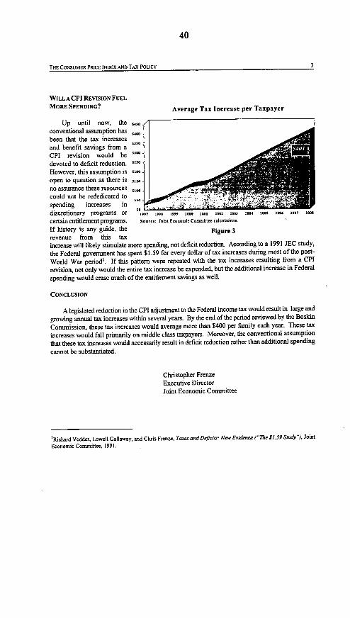
40
THE CONSUMER PRICE INDEX AND TAX POLICY 3
WILL A CPI REVISION FUEL
MORE SPENDING? Average Tax Increase per Taxpayer
Up until now, the .s..conventional assumption has
been that the tax increases
and benefit savings from aCPI revision would be SS0Odevoted to deficit reduction. s""However, this assumption is szoo
open to question as there is ,,,no assurance these resources ..00
could not be rededicated to :. X
spending increases in
discretionary programs or 9, , ,.. , 2" o 0000 200 200 2004 2007 000W
certain entitlement programs. So-.: JOil Ecoo...ic commaitoe oaulnliot..
If history is any guide, the Figure 3
revenue from this taxincrease will likely stimulate more spending, not deficit reduction. According to a 1991 JEC study,
the Federal government has spent $1.59 for every dollar of tax increases during most of the post-
World War period'. If this pattern were repeated with the tax increases resulting from a CPI
revision, not only would the entire tax increase be expended, but the additional increase in Federal
spending would erase much of the entitlement savings as well.
CONCLUSION
A legislated reduction in the CPI adjustment to the Federal income tax would result in large and
growing annual tax increases within several years. By the end of the period reviewed by the Boskin
Commission, these tax increases would average more than $400 per family each year. These tax
increases would fall primarily on middle class taxpayers. Moreover, the conventional assumption
that these tax increases would necessarily result in deficit reduction rather than additional spending
cannot be substantiated.
Christopher FrenzeExecutive DirectorJoint Economic Committee
'Richard Vedder, Lowell Gallaway, and Chris Frenre, Taxes and Deficits: Nei-Evidce ("eSTh ]. 59 Study'), Joint
Economic Committee, 1991.

41
PREPARED STATEMENT OF COMMISSIONER ABRAHAMMr. Chairman and Members of the Committee:
I appreciate this opportunity to comment on the labor market datareleased this morning.
Unemployment declined in April, and nonfarm payroll employmentrose. The unemployment rate dropped by three-tenths of a percentagepoint to 4.9 percent; over the prior 10 months, the rate had remained ina narrow range from 5.2 to 5.4 percent. Payroll employment increasedby 142,000 in April, about the same as in March (as revised), but wellbelow the growth realized in January and February. Unfavorableweather during the survey reference periods dampened constructionhiring in both March and April.
In April, employment in the services industry increased by 93,000.There were relatively large over-the-month gains in health services,Social services, and engineering and management services. Job growthin computer and data processing services continued at its steady pace.In all these industries, employment has been on an upward trend formany years. Partly offsetting these increases in April was a decline inamusement and recreation services. Help supply services showedvirtually no change in employment in April. Although this industry hasbeen a major contributor to job growth during the six years of thecurrent economic expansion, gains since last August have been bothmore modest and more sporadic.
In April, each of the major components of finance, insurance, andreal estate added jobs, and employment also continued to rise intransportation and communications. In retail trade, a gain in eating anddrinking places was partly offset by a decline in general merchandisestores.
In manufacturing, employment declined by 14,000 over the month,reflecting, in part, a strike in auto manufacturing and some temporaryshutdowns for inventory control in that industry. From September toMarch, factories had added 75,000 jobs. In April, growth continued inindustrial machinery, fabricated metals, and aircraft. Also, overallmanufacturing hours rose to match its post-World-War-II high level, at

42
42.2 hours, and overtime edged up to 5.0 hours, its highest level since
the series began in 1956.
In April, construction employment declined for the second month in
a row. Following a large gain in February, employment in the industry
has decreased by 69,000 over the past two months, on a seasonally
adjusted basis. Bad weather across much of the country during the
March and April survey reference periods probably delayed some of the
normal hiring that we would have otherwise expected to see during
those months.
Average hourly earnings edged down by a penny in April. This
followed increases totaling 11 cents over the first quarter of the year.
Although the month-to month movements in this data series remain
quite volatile, the over-the-year gains for recent months clearly have
been running higher than during the early part of 1996.
The 4.9 percent unemployment rate in April was the lowest since
1973. The number of unemployed persons declined to 6.7 million. All
the major demographic groups contributed to the decline in the overall
jobless rate, and the unemployment rates for both whites and blacks and
for adult women were down significantly. Unemployment decreased
among those who had been looking for work for less than 14 weeks and
among those who had lost jobs to which they did expect to be recalled.
Although a great deal of attention will undoubtedly will be paid to the
drop in the jobless rate, I would caution, as always, against reading too
much into any one month's data.
Total employment, as measured by our household survey, was
essentially unchanged in April. The proportion of the population with
jobs (the employment-population ratio), however, remained at a record
level of 63.8 percent.
In summary, unemployment fell in April, and payroll employment
rose modestly. The employment-to-population ratio, manufacturing
hours and manufacturing overtime all remained at historically high
levels.
My colleagues and I now world be glad to respond to your questions.
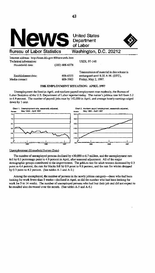
43
S | United States
% 41 e w s Department
Bureau of Labor Statistics Washington, D.C. 20212Internet address: http://stats.bls.gov:80/newsrels.htmTechnical information:
Household data: (202) 606-6378
Establishmentdata:Media contact:
Transmission of material in this release is606-6555 embargoed until 8:30 A.M. (EDT),606-5902 Friday, May 2, 1997.
THE EMPLOYMENT SITUATION: APRIL 1997
Unemployment declined in April, and nonfarm payroll employment rose modestly, the Bureau ofLabor Statistics of the U.S. Department of Labor reported today. The nation's jobless rate fell from 5.2to 4.9 percent. The number of payroll jobs rose by 142,000 in April, and average hourly earnings edgeddown by 1 cent.
Chan 1. Unemployment rate, sea99al9 adjusted,vow,~i May 1994 -Apnl 1997
5.0 \oo,,,I. . . . I .. . . . .,
*996 *995 *S9
Chan 2. Nontattt paymrt: emplyrment seasonaty adjusted,a May 1994 -Apri 1997
110
00 '. , , .. . .. I . .. . .. .. . ., , I . . .. .. .. ..I .1955 *598 *ss
Unemployment (Household Survey Data)
The number of unemployed persons declined by 430,000 to 6.7 million, and the unemployment ratefell by 0.3 percentage point to 4.9 percent in April, after seasonal adjustment. All of the majordemographic groups contributed to the improvement. The jobless rate for adult women decreased by 0.3point to 4.4 percent, the rate for blacks fell by 0.9 point to 9.8 percent, and the rate for whites droppedby 0.3 point to 4.2 percent. (See tables A-I and A-2.)
Among the unemployed, the number of persons in the newly jobless category-those who had beenlooking for work fewer than 5 weeks-declined in April, as did the number who had been looking forwork for 5 to 14 weeks. The number of unemployed persons who had lost their job and did not expect tobe recalled also decreased over the month. (See tables A-5 and A-6.)
USDL 97-148

44
2
Table A. Major indicators of labor market activity, seasonally adjusted
(Numbers in thousands)
Quarterly averages Monthly data Mar.-
Category 1996 1997' 1997' Apr.
I Feb. I Mar. I Apr. change
HOUSEHOLD DATA Labor force status
Civilian labor force...........................
Employm ent...............................
Unemployment............................
Not in labor force..............................
All workers........................................
Adult men...................................
Adult wom en...............................
Teenagers....................................
W hite...........................................
Black...........................................Hispanic origin............................
ESTABLISHMENT DATA
Nonfarm employment .......................
Goods-producing'.......................
Construction...........................
M anufacturing........................
Service-producing' .....................
Retail trade.............................
Services..................................Governm ent...........................
Total private......................................
M anufacturing.............................
Overtime.................................
Average hourly earnings,
total private..................................Average weekly earnings,
total private..................................
1'
134,830 135,934 135,634 136,319 136,098 -221
127,705 128,728 128,430 129,175 129,384 209
7,124 7,206 7,205 7,144 6,714 -430
66.627 66,462 66,754 66,194 66,577 383
Unemployment rates
5.3 5.3 5.3 5.2 4.9 -0.3
4 4 4.5 4.41 4.4 4.2| -.2
4. 1 4.7 4.71 4.71 4.4| -.3
16.6 17.0 17.5 16.1 1 5
.4
-1.0
4.6 4.5 4.5 4.5 4.2 -.3
10.6 10.9 11.3 1 0
.7 9
.8
-.9
8.0 8.3 8.1 8.6 8.1! -.5
Employment
120,509 p121.238 121,296 p121,4
35 pl2
1.577 p14 2
24,320 p2 4
,4 6 9
24,508 p24,499 p24
,4 4 2
p-57
5,492 p5.596 5,639 p5,61
4p5,5
7 0p-44
18.262 p18,304 18,299 p1 8
,3 1 6
p18,3 0 2
p.14
96,189 p96,769 96,788 p96,936 p97,135 p1 9 9
21,864 p2 1
,9 5 2
21,940 p2 1
,9 9 3
p22,0 2
5 p3 2
34,785 p35,096
35,101 p35,17 3
p35.2 6 6
p93
19510 p19557 19,577 pl9,550 p19,582 p32
Hours of worka
34.6 p3 4
.7
34. p3 4
-9
p3 4
.6
41.84 1.
1. 41.9 p42.1 p42.2
4.5 p4.8 4.7 p4.9 p5.0
p-0.3
P1P.1
Earnings'
$11.98 p$l2.101 $12.10 pS12
.15 p$12.14 p-$0.0 1
414.00 p419.48[ 422.29 p424.04 20.04 .00
' Beginning in January 1997, household data reflect revised population controls used in the survey.2 Includes other industries, not shown separately.' Data relate to private production or nonsupervisory workers.p=preliminary.
_ _. ... .. _ . . .. . .: .
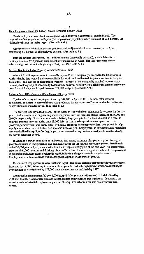
45
3
Total Employment and the Labor Force (Household Survey Data)
Total employment was about unchanged in April, following a substantial gain in March. Theproportion of the population with jobs (the employment-population ratio) remained at 63.8 percent, thehighest level since the series began. (See table A- I.)
Approximately 7.9 million persons (not seasonally adjusted) held more than one job in April,comprising 6.1 percent of all employed persons. (See table A-9.)
Both the civilian labor force, 136.1 million persons (seasonally adjusted), and the labor forceparticipation rate, 67.2 percent, were essentially unchanged in April. The labor force has shownsubstantial growth since the beginning of last year. (See table A- l.)
Persons Not in the Labor Force (Household Survey Data)
About 1.5 million persons (not seasonally adjusted) were marginally attached to the labor force inApril-that is, they wanted and were available for work, and had looked for jobs sometime in the prior12 months. The number of discouraged workers-a subset of the marginally attached who were notcurrently looking forjobs specifically because they believed nojobs were available for them or there werenone for which they would qualify-was 379,000 in April. (See table A-9.)
Industry Payroll Employment (Establishment Survey Data)
Total nonfarm payroll employment rose by 142,000 in April to 121.6 million, after seasonaladjustment. Job gains in many of the service-producing industries were offset somewhat by declines inconstruction and manufacturing. (See table B-l.)
The services industry added 93,000 jobs in April, in line with the average monthly change for the pastyear. Health services and engineering and management services recorded strong increases of 34,000 and29,000, respectively. Social services had a relatively large job gain for the second month in a row. Incontrast, business services added only 19,000 jobs, as continued expansion in computer and dataprocessing employment was partly offset by a small decline in help supply services. Job growth in help
supply services has been both slow and sporadic since August. Employment in amusement and recreationservices declined in April, reflecting, in part, slow seasonal hiring due to unusually cold weather duringthe survey reference period.
In April, job growth continued in finance and real estate; insurance also posted a gain. Strong jobgrowth continued in transportation and communications for the fourth consecutive month. Retail tradeadded 32,000 jobs in April, somewhat below the average monthly gain of the past year. An employmentincrease of 46,000 in eating and drinking places offset a loss of similar magnitude in March. Employmentin general merchandise stores declined in April, following a large increase in the prior month.Employment in wholesale trade was unchanged in April after 2 months of growth.
Government employment rose by 32,000 in April. The noneducation component of local governmentincreased by 19,000, following 2 months without growth. Federal employment, which was unchangedover the month, has declined by 275,000 since the most recent peak in May 1992.
Construction employment fell by 44,000 in April (after seasonal adjustment); it had declined by25,000 in March. Unfavorable weather in both months contributed to this weakness. In contrast, theindustry had a substantial employment gain in February, when the weather was much warmer thannormal.

46
4
Manufacturing employment declined by 14,000 in April, following again of 75,000 over the prior 6months. Motor vehicles and equipment lost 13,000 jobs in April, mostly due to temporary shutdowns forinventory control and a strike of 3,500 workers. Employment growth continued in industrial machinery,fabricated metals, and aircraft; gains in these three industries totaled 14,000 over the month and 102,000over the past year.
Weekly Hours (Establishment Survey Data)
The average workweek for production or nonsupervisory workers on private nonfarm payrolls fell by0.3 hour in April, to 34.6 hours, seasonally adjusted. The manufacturing workweek edged up by 0.1 hourto 42.2 hours, matching its post-World War E high reached in January 1995. Factory overtime edged upto 5.0 hours, the highest level since the series began in 1956. (See table B-2.)
Reflecting the decline in the average workweek, the index of aggregate weekly hours of privateproduction or nonsupervisory workers on nonfarm payrolls dropped by 0.8 percent to 139.6 (1982=100)in April, on a seasonally adjusted basis. The manufacturing index, in contrast, edged up by 0.2 percent to107.6. (See table B-5.)
Hourly and Weekly Earnings (Establishment Survey Data)
Average hourly earnings of private production or nonsupervisory workers edged down I cent in Aprilto $12.14, seasonally adjusted, following gains totaling 11 cents in the first quarter. Average weeklyearnings were down 0.9 percent to $420.04 in April. Over the past year, average hourly earnings haveincreased by 3.6 percent and average weekly earnings by 4.5 percent. (See table B-3.)
The Employment Situation for May 1997 is scheduled to be released on Friday, June 6, at 8:30 A.M.(EDT).
Revisions in the Establishment Survey DataThe Employment Situation news release of May data in June will introduce revisions in
the establishment-based series on nonfarm payroll employment, hours, and earnings to reflectthe regular annual benchmark adjustments for March 1996 and updated seasonal adjustmentfactors.
This year's benchmark process affects all unadjusted series from April 1995 forward. Inaddition, the unadjusted data from January 1988 forward for selected series in the transporta-tion and public utilities division will be revised to reflect industry coding changes for a groupof employers within the airline and trucking industries. These recomputations will have aslight effect on higher level aggregate series, including total nonfarm employment.
All seasonally adjusted series will be revised from January 1988 forward to incorporatean updated version of the X-12 ARIMA seasonal adjustment software. Seasonal adjustmentfactors for March through October 1997 will be available on May 30, 1 week prior to therelease of the May estimates, on the Internet (http://stats.bls.gov:80/ceshome.htm) or bycalling (202) 606-6555.

47
Explanatory Note
This sews elease presents statistics from two major surveys. theCurrent Population Surey (household survey) and the Curreot
Employment Staistics survey (establishment survey). The household
surey provides the information on the labor force, eiployment. and
unemployment that appears in the A tables, marked HOUSEHOLD
DATA. It is a sample survey of about 50.000 households conductedby the Bureau of the Ceosus for the Bureau of Labor Statistics (BLS).
The establishment survey peovidrs the information on theemployment, hours, and earnings of worke us on sofarm payrolls that
appears in the B tables, marked ESTABLISHMENT DATA. This
information is collected from payroll records by BLS in cooperarioswith State agencies. In June 1996. the sample included about 390.000
establishments employing over 47 million people.For both surveys. the data for a gives month relate to a paricular
week or pay period. Is the household survey. the reference week is
generally the calendar week that contains the 12th day of the month. In
the establishment survey, the reference peiod is the pay peiodincluding the 12th, which may or may not correspond directly to the
calendar week.
Coverage, definitions, and differences
between surveysHousebold survey. The sample is selected to reflect the enutre
cinilian nonimtitutional population. Based on responses to a senes of
questiom n work and jobsearch activities, each person 16 years andover in a sample household is classified a employed, unemployed. or
not in the labor force.People are classified asemploydif they did any work at all as paid
employees during the reference week: worked in their own business.profession. or on their own fans, or marked without pay at least 15
hours infamily businessorfarm. Peoplenrealocoumed asemployed
if they were temporaily abtset fomm thetjobsbecauseof illness, badweather, vacation, labor-management disputes, or personal reasons.
People are clssified asunrployed ifrhey meet all of the followingcriteia: Thy had noemploymentdoriegthe reference wk: they were
available for work at that time; and they made specific efforts ta find
employment sometime duaing the 4-week period ending with the
referenceweek. Personslaidofffnm a joba-denpectingrecall need
ntbelowkingforworktobeco-Medasunemployed. The-uemploymentdata derived from the household survey in no way depend upon the
ehgibility for or receipt of unemployment insurance benefits.
The civilian labhrforre is the sum of employed and unemployed
persons. Those not classified as employed or unemployed aremn in the
laborforce. The uaemploymen crle is the number unemployed . apercent of the labor force. The latb.force pnicipuo.n rate is the
labor force as a percent of the population, and the employee-
populairo ratio is the employed as a percent of the population.
Buoablislsmentsmrrey- The sample establishments are drawn frompovate nonfarm businesses such a factories, offices, and stors.as well
as Federal, State. and local govermmententities. Earploy-eeon sorfaou
payrolls are those who received pay for soy part of the reference payperiod, including persons on paid leave. Persons an coumted in each
job they hold. Hournand ena-ingsdata-am for povam bosinesnesoandmime only to producuon workers in the goods-prodacing sector and
auosuperviscry workers in the sorvice-prduacng sectorDifferenets in employment estimates. The numerous cooLeptual
and methodological differences between the household andstablishmemsurveysresultinimpornantdistictiosiintLheemploymem
esomates derived from the surveys. Among these are:
* The household survey includes agricultural workers. the self.
employed, unpaid family workers and private household workers among
the employed. Thee groups aenxcluded from the etablishount urvey.* The household survey irnludes people so unpaid leave among the
employed. The establishment survey does am.
* Thehouseholdsrveyis limitedio onksers 16years-fageandolder.
The establishment survey is not limiated by age.* The household surey has no duplication of individuals. because
individuals sue counted only once, even if they hold more than onejob. Inthe establishment survey, employees wurking at more thas one job and
thus appearing on more dhai one payroll would be counted separatly foreach app-ence.
Other differences between the two surveys are described in
"Comparing Employment Estimates from Household and Payroll
Surveys." which may be obtained from BLS upon request.
Seasonal adjustmentOver the course of a year. the nice of the nation's labor force and
the levelsofemploymentanduoemploymentendergoshamfpluctuatiomsdue to such seasonal events as chauges in weather, reduced or
eupanded poduction, harvests, major holidays. and the opening and
closing of schools The effect ofsuch seasonal vasiationcas be verylarge: seasonal flucuations may account for as much as 95 percent of
the month-to-month changes in unemployment.Because these seasonal events follow a more or less regular pattenm
each year, their influence on statistical trends can be eliminated by
adjusting the statistics from month to month. These adjustments make
nonseasonal developments, such a declines in economic activity or
increases in the participation of women in the labor force. easier to
spot. For example, the large number of youth entaing the labor forceeach June is likely to obscure any other changes that have taken place
relative to May, making it difficult to determine if the levl of
econouic activity has sn or declined. However. because the effectof students finishing school in prerious years is knows, the statistics
for the current year can be adjusted to allow fora comparable change.
Insofar as the seasomnl adjustment is made orrectly, the adjustedfigure provides a more useful tool with which to analyce changes ineconomic activity.
Is both the household and establishment surveys. most seasonally
adjusted seris are independently adjusted. However, the adjustedseris for many major estimates. such a total payroll employment,
employment in most major industry divisions, toaI employment. and
unemployment are computed by aggregating independently adjustedcomponent series. For enample, total usomployment is derived by
summing the adjusted series for four major age-ur components: this
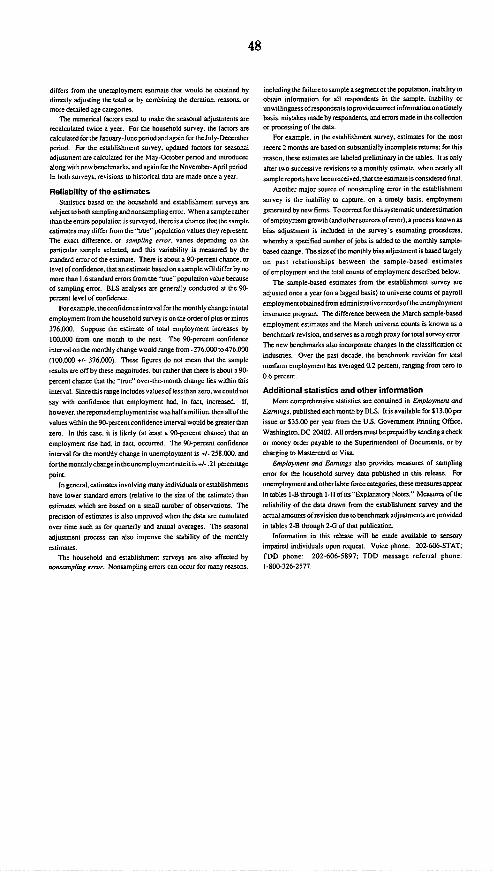
48
differs from the unemployment estimate that would be obtained by
directly adjusting the total or by combining the duration. reasons. or
more detailed age categones.
Tbe numenscal factors used to make the seasonal adjustments are
recalculated twice a year For the household sorvey, the factors are
calcolatedfortheianuary-Jane penod and agaio forthe July-December
period. For the establishment survey. updated factors for seasonal
adjustment are calculated for the May-October persod and introduced
along with new benchmarks, and again for the Novembe ,April penod
In both surveys, rvisions to histotical data ae made once a year.
Reliability of the estimates
Statisncs based on the household and establishment surveys ae
subject to both sampbing and nonsampling error. When a sample rather
than the entire population is sorveyed. there is 3 chance that the sample
estmates may differ from the "tue' population values they represent.
The exact difference, or ampling error, varies depending on the
particular sample se[leted, and this vanability is measured by the
standard error of the esumale. There is about a 90-percent chance, or
level of confidence. that an estimate based on a sample will differ by no
more than 1.6 standard errors from the "iron" population vale because
of sampling error BLS analyses am generally conducted at the 90-
penmeno level of confidence.
Fouexampletheconfidence interval forthemonthly change in total
employment from the household survey ison the order of plus or minus
376,000. Suppose the estimate of total employment increases by
100,000 from one month to the next. The 90-percent confidence
interval on the monthly change would range from -276.000to476,000
(100,000 +/- 376,000). These figures do not mean that the sample
results are off by these magnitudes. but rather that there is about a 90-
percent chance that the "true" over-the-month change lies within this
interval Sincethisrongeincludesvaluesoftessthan zero, we could not
say with confidence that employment had, in fact, increased. If,
however. the meponed employment ise was halfa million, then all of the
values within the 90-percent confidence interval would be greater than
em. In this case. it is likely (at least a 90-penent chance) that an
employment rise had, in fact, occured. The 90-percent confidence
interval for the monthly change in unemployment is +/. 258,000. and
forthe monthly change in the unemployment rnote it is +-.21 percentage
point.
In general. estimates involving many individuals or establishments
have lower standard emons (relative to the sim of the esamate) than
estimates which are based on a small number of observations. The
precision of estimates is also improved when the dam am cumulated
oven nime such as for quarterly and annual averages. The seasonal
adjustment process can also improve the stability of the monthly
estimates.
The household and establishment surveys ame also affected by
non-ampling error- Nonsampfihg errors ran occur for many reasons,
including the failure to sample a segmentof the population. inability toobsain inforsaton for all respondents in the sample. inability or
unwillingnessofrespondenLstopmidecorrectinfontnaiononatmelybasis, mistakes made by respondents, and enors made in the collectionor processing of the data
For example, in the establishment survey, estimates for the most
recent 2 months am based on substantially incomplete remms: for this
reaso, these esumates are labeled preliminary in the tables. It is only
after two successive revision to a monthly estimate. when nearly all
sample reports have been received, ham theestimate isconsidered final.
Another major source of nonsampling eror in the esutabshment
survey is the inability to capture. on a imely basis. employment
generated by new firms. To correct for this systemaac underestimation
of employment gowth (and othersources oferor). a process known as
bias adjustment is included in the survey's esimating procedures.
whereby a specified number of jobs is added to the monthly sample-
based change. The si of he monthly bias adjustment is based largely
on past relationships between the sample-based estimates
of employment and the toet counts of employment described below.
The sample-based estimates from the establishment survey are
adjusted once a year (on a lagged basis) to universe counts of payroll
employmentobtained from administrative records of theunemployment
insurance program. The difference between the March sample-based
employment estumates and the March universe counts is known as a
benchmark revision, and serves as a tough pnoxy for total survey ernor.
The new benchmarks alto incorporate changes in the classification of
industries. Over the past decade, the benchmark revision for total
nonfam employment has averaged 0.2 percent, ranging from rem to
0.6 percent.
Additional statistics and other information
More comprehensive statistics are contained in Eiipluy-eni and
Earninga, poblished each month by BLS. It is available foS13.00 pen
issue or $35.00 per year from the U.S. Government Printing Office,
Washington, DC 20402. All orders must b prepaid by sending a check
or money order payable to the Superintendent of Documents, or by
charging to Mastercard or Visa.
Employnsenr and Eareorgs also provides measures of sampling
eror for the household survey data published in this release. For
unemploymero and other labor force categories, these measumrs appear
in tables Il-B through I -H of its 'Explanatory Notes." Measures of the
reliability of the data drawn from the estabbshmeM survey and the
actual amounts of revision due to benchmark adjustments amprovided
in tables 2-B through 2-G of thau pubbcation.
Information in this release will be made available to sensory
impaired individuals upon request. Voice phone: 202-606-STAT:
TDD phone: 202-606-5897; TDD message referral phone:
I-800-326-2577.
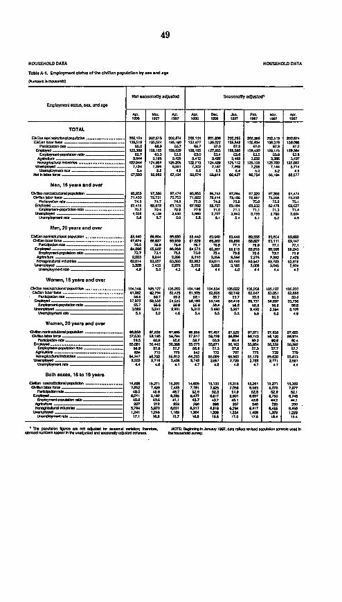
49
HOUSEHOLD DATA HOUSEHOLD DATA
To 1 A-1. Epk-M t 9 10 1 D 9999999019 pop91910f by sex end age
Not Seasnlly9ao5std so....y 981a9usteoI
Eo96p9oy91 sl s16 .99, a,1d ago
0 I7.1 9. I. F. r . . F- I .39 1967 1 1997 1996 J 99w 9 997 1997 ID97
TOTAL
C9,00,199,099613699TOTAL 20O.101 291593 20.674 299101 201.636 20285 299.339 29Z.13 2029.74r9091M.II6919 139,512 135,52. 135.19 1933.427 135r 135.848 9355.63 136,319 135,09.
P9,193.8990999 m56.2 96.9 r6.7 69.7 67.0 672 673 67.3 67.269089y99 _91J236 120.125 12.69 926.125 17V355 9205,90 92.39 1 290.75 129.36
EO6*s, mc 62.7 63.3 63.5 63.0 634 63.9 6r3.5 63.0no .9A514011999 3.394 3.166 3920 3.412 3.926 3.230 3 r 13.6 3.907
14992996959999649969999 9229 92,959 925.29 122.73 124.429 120112 125.139 I25.79 9250 766.76d994 1 7.124 7.329 6.10 7.fl 7.167 7.269 7.20 7.94 6.714
161951519p5999 rc99 _________________ 5.4 5.5 43 5.5 3 s .4 5J3 52 4*9MI996b96 r7Ps5s 66,989 67.4 49 68.674 rsss4 9r437 65,754 66.195 66.577
Men, 16 years and over
r9 n p O 95.95 97.386 97.474 e6.9s 9`.742 97W.204 07 0 97.396 97.474Cb 96 9 k990 79.909 7.731 72.750 71.92 7Z4914 73.196 7299Z 7 73.268 73.2
PwlcO n9a' 1991 74.5 74.7 74.6 75. 74.9 75.2 75.0 75.2 75.106989|99 67.415 66.573 69.105 67.932 69.707 r9.194 W=.22 69.478 69.627
E919019,n99999-9996699I1,,,9 20.3 70.4 702 70' 71.0 7191 719. 79. 719.I74.03 45,1a 3.650 3.990 3.707 3.942 3,755 3.790 3.690
169999830.669090 .9ss 5.7 s0 50 9.1 5. 5.9 5.2 4.9
Men, 20 years and over
096f5ro9996699 p966f9369 89440 s9.694 89600 09.0 9.040 95.449 89.554 S9,04 859.90r0 b16 b6 9 67.924 6.957 66.S3 67.999 66.369 6.3998 69927 69.11 9 r.147
P99lcp99io,9 9969 76 79.9 76.9 79.7 75.9 77.1 79.9 77.9 77.1E,1989wd r.06439 60092 6s930 69.573 6.367 63.13 69.818 66.06s 66,243
ECo p .pd6 98 73.7 73m1 73.0 76 73.4 73.6 75 73.7 73n9Ag*W9 2.23 2.24 2.396 2.310 2359 2,364 2276 2.362 3.2N9 93 9.4,L09i9 62.61 63o257 63.560 620r3 63.099 6&3.49 3.542 63.703 63.815
93997b690d 3.35 3.9045 2.976 3356 3= 3.185 3AD9 36045 2.994u9n.9198,I5,:0n9, 4.9 3.0 4.3 4.9 44 4.6 4.4 4.9 42
Women, 16 years and over
rO1 n6ft rPOPW 10949M *os.127 105.200 1049149 90435 ICS. IMAM 9.1927 905926ri09,639 95b 9 61.0 62.79 62.426 61595 62.D 62 742 62647 63.061 62366
Pa99 MIe. 59.9 59.7 595 59.1 59.7 59.7 596 60.0 o 96D57.973 50.552 59.525 59.193 59,149 59.416 59.197 59.7 59.756
E996r-9*.,9 969 55.7 569. 56.6 55.9 59.4 50.6 s 569 9e.1666 7d._ 3.089 3.241 2.901 3,312 3.490 3.327 3.50 3.54 31
u6989,9119 5. 1 52 4* 5.4 55 5.3 53 5.3 49
Women, 20 years and over
r 9 9 9121 9 5p6 _ _ 96MAsS 9763 67.685 9Sal5s 07,457 677520 67,571 7.638 W7A6S0r99 b96669699 57.636 5 59.7D 9 9739117 59.7029 5UN 56.743 59.1*3 s9.79
ftftk t,9 99.5 60.6 602 59.7 69.3 G6M 6.02 6.6 60.4E998o4d4 55- 31 56.492 56.399 55.075 5537 9.165 55.954 56.359 5639
Br99p9.VM9 9 foU 069 W79 57.7 549. 57.3 57J 57.3 57.7 57.7Ag9t999 834 710 775 642 772 797 775 739 779Nl-gft996 W 699A. 594247 55.732 55.913 54233 55.909 650369 55.179 55.2 55,.13
69199996954 2.555 2.716 2aD9 27a2 2.657 29 2.788 2.771 2.599Wn0O 9 9ta 4.4 4.6 9.9 4.7 49 43 4.7 4.7 4.4
Both sexes, 16 to 19 yeara
9X9 n9r9 o n4- | 9996 19 271 J5.309 M4.9N5 139 15.318 95.2I 95271 15,90r01 b69 19 7252 7.420 7.453 7.731 7J75 7.906 e .os5 4.079 7J77
P96P1991 n9o 49.0 46. 49.7 52.6 523 519 523 92.9 521E.Op694 60991 6.1s2 6205 6.477 9317 6.6D9 6.657 6.750 6.749
E.*bp .999p 99 9b91 40.9 6.0 491.1 43.7 437 43. 43 44.02 ".A UW49 92 727 212 M 2379 296 307 240 25 7iN a dFhff9s b96. 5.76 5.970 6.91 6217 6.319 6294 6.417 6.465 6.458
_. __ _ _._ 1.241 124 1.169 1.4 1*x 1J54 1.4I0 1.= 279999990p9o19 a99 17.1 I63 15.7 163 96.5 17.0 i7.5 16.4 91.
'9. TVbJion fig- -mr 699 W 999 990. 6.9.. NOTE9.6.9h4 Ih J-ary 1907.96941199499d49,AW9940999us699hUn09 99919deed99998or69939*X984999994999990S*164y09,99 9BY,99 t.. 96b 7.
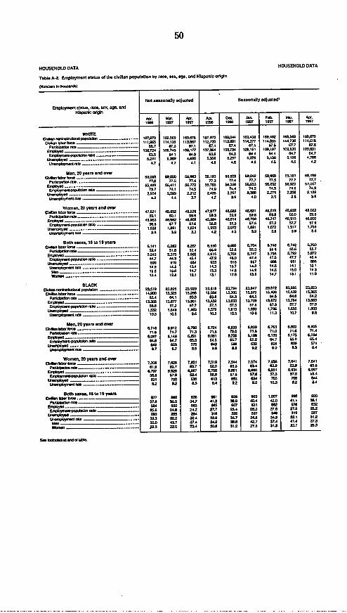
50
HOUSEHOLD DATA HOUSEHOLD DATA
Table A.2. Employment 9 of tlofl pop9dl00n by sac, 000. 0ge nd Otopooto otglo
(0.00 0 * .:*)
Not o"oily odjootod S.-.ooflty .,-tod9
Ho*940019 _ _ __40. 0m. m..0a9. 0 F , age. . A.
.me 997 I"?7 900 10 90 97J99]9
WolTEClm, 9900090950 907.073 99900_ 90007 907.07 004 90..3 199.409 900.0 9.7
CoON. 0905 99.135 993.07 912.720 93.9 994.A77 194.333 194.738 194.618p 99bp9 90.7 7 07.o9 67.1 07.4 I7.5 I7. 07.7 67.0
e40290|0 900.724 .705 909.177 907.34 9097643 1 4.4 909...9 9 .037 &4.7Er~~p099990.000940099 000 0~~3.5 GM. 64.3 SIR 43 04 40 047 0.
050nwpyod 5.241 53e 4.90 w .2GA7 56 05.93 5.105 4.700
uthdr-a W 4. 07 4.9 4.8 4.0 4.0 4.5 4.5 .2
Mo. 20 004 oWGG_ t0 SUM * 900s) 0M 90.903 04& . 90.002 MM 90.901 053940
ftftol m"A . 77. 77 7.4 77 n774 77.7 77. 7.7 7.7
Eo00W90 05.409 9.99 564 4 5.773 00.765 50200 00.053 00.00 5-Me 5-7.0
E~~op~oyl.900.0op00l 90909 ~~~~73.7 74.9 0. 74. 0 C 74.0 74.0 74.5 74. 74.9.
009.9099984 . Z-2.0 2.500 2.212 2.020 2. 2. .300 2.275 2.23 2.93
I h-br o 900 4.3 04 3.7 4.2 3. 40 3.0 3.0 3.6
WBot , 2070e 790 0'd
C _e bb. 900 47.029 04.0 0.e5; 47.097 0.00C 40.031 45.090 40.3 48.02
e t_00990........ ..2 -| 9 00.391 090 005 000 50.03 90. 0.0 00.0
09190909984 00.003 40.0962 E 492 0.4 40.010 40750 40.747 40.090 40.o H
e,9o0990000.00900920 9010 00.0 577 570 00.0 573 07.0 57.0 57.7 07.0
W=lowo n 1.3 9.09 1.024 9993 Z.572 I.009 10723 I917 I.753
00,9009799.90 - 3.0 3.9 3.3 4.2 423 3. 3.0 &3. 3.6
Both 80099.160to107y099
CWe III 0 61410 0202 0.357 050 = 0.704 6.746 6.702 60.700
P00094.09991000 52.~~~~~~~~~4 09.0 04 03.9 5500 03.3 950. 5506 50.7
e r00900.4 0202 5.373 00 5.615 5.7 5.747 5.759 0.799 5072
E.001091Tds0.7009009019 4.7 003 03.0 47.0 00.0 474 47.0 47.7 40.0
Women,09054 000 0~s e10 004 930 090 007 000 059 .60000090959-9 900..9.0 94.5 93.0 943 37 942 140 941 3.
___ 95.0 9. 14.7 95.3 4.0 94. 14 19 94
_________oth __________________ _ 13." 1 S4 93.0 12. 93. 92. 9 14 .7 93I9 99.0
BLACKC9.0009_ 0909 923.90 23.00 23.9 23.509 23.704 0000 23 .073 23.8000U 23.3
CO.00400099000 . 9~~~~~~~~~4.09W is-V 10.0 90.004 90.3M IS.3= 95.408 95.439 I0.30
a000t.0gr49090 03.4 04.9 G" 03. 604 60.5 6452 6006 642
t0d0790084 13.368 3.7 13.801 4342 23 376 9 3,03 6 3.704 93.003
Eoo09ol9009009900l00 9. - - - 00.0 572 57.7 57.1 075 97.0 0723 57.7 59
U-qby0709d 1.532 1I04 1.463 9.07 10913 Jim0 9.730 1A0 I.00
9me0909,0 000 - ~~~~ ~~~~~~1023 10.0 0A 13. 90.0 9.0 112 93.7 0.0
MMts 20 yaG,,,.d4 0Q.
ChiomeIftO00 ,790 0.092 0.790 0.724 0.00 0.029 0i.70 O.90 0.809
p099~~~~~99099990 ~~~~~~79.0 79.7 79.3 79.0 73.0 79.0 71.0 7906 71.4
00009084 0.00~~~~~~~~~~~6,7 0.194 0.23 0.09 0.23 G.90 0.150 0.173 0.209
E09009010090000900001 9000 0~~~~4.0 09.7 03.3 000 05.7 0W. 04.7 05.0 654
00900090980 040~~~~~~~~~~e so3 575 003 000 32 am0 an 971
90~~9900O 9098 __________________ ~ 0.7 9.7 0.0 Le0. 0.2 00 0.3 0,4
W009000. 200YoII,, so oowC~ 9 007.= 7.028 7.319 7.310 7?4 7.974 7.030 7.041 7.049
P019 9890 __________________________ 09s 837 937 MD. G". 93.4 63..9 09 63.8
05o09o~~~~~~~~84 0.7~~~~~07 0.0S 0.997 0.79 0.00 0.00 0.001 0.030 0.097
lobo900B0090990 50. 07.0 00.0 90. 5705 070 57M 97 00.4
009.9~~~~~~~~~o84 0~~~~~01 700 030 093 003 004 700 70 604490-0997990900 8.G2 0.2 0.3 04 02 02 90.2 02 0.4
Both -80I000.10051070090CbW bbt S"0 7 00 83 999 22e 900 127 990 200
P00~~~~~~9 9090 ~~~~~~~370 30.5 34.7 4193 310.9 40,4 42.0 41.9 30.9E
9 ~.OW 994 Sao 503 045 607 031 002 070 032E7000951990-9009009009 9000 00.0~Z5L 2405 24.2 271.7 20.4 09.3 2706 2709 25.2- ~~~~ ~~~~ ~~~~~~~~~283 200 254 390 322 337 340 390I 207
00 ,7990000 32.3 32.2 30.4 3. 347 30.0 34.3 32.9 391
00.9 30.0~ ~~~~~~~~~~~~ 43.7 374 34.0 300 03.7 37.4 09.4 372PS. 23.0 23.4 30.1 392 27.5 312 207 2023
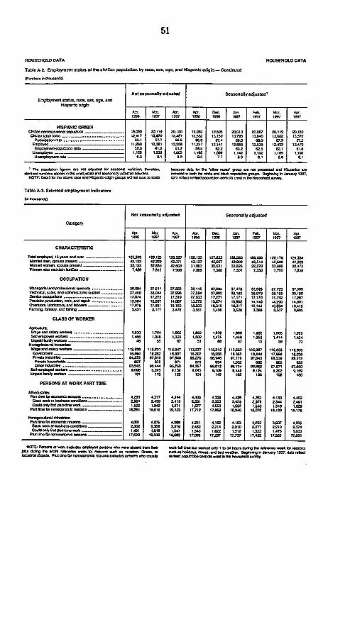
51
HOUSEHOLD DATA
Tab09 A-2. E999p!oy..d 091h 9 d of t Mli0 m pp lti.n by 9.e, 990 .g9 .999 Hipa799 odgi0 7- Co99999
Cur 99 i 0 no
HOUISEHOLD DATA
Not os-as99ly odjuwted S a on.y adJu ted'E,, t s't-lus.ya, r. sGo age, and
AMl. M.~. AP'. AP. D-e .2.kt9 .90. AP.196 1997 1997 1996 199S 1937 l997 aw 1997
HISPANIC ORIGINt7 r l 9998090119.990 20.19 2190 199 15.9 20.013 20.097 29.119 20.19eCto29 t Ie 1 .917 I3.W 19.27 123992 19.990 13.79 13a6 13.612 13572
999.91939011919 69~~~~~~-1 67.7 60. 699 7 9. a". 62.9 97.3Emrpbod~ 611.9 12.391 123.99 115957 12.141 12,653 12.w33 126493 12.970E,1oopo99.p~799 9.90o90 61.5 692 99 622 6.2 6zs. V-i 61L
U-9,p9d 1.15 1239 1.069 1.195 .M09 1.12 1.199 1.199 1.199U6-069 -,99 9.3 9.1 .0 9.5 7.7 0.3 &I a.6 &I
Th. P91t9, fg0. 9 -9 _I9tor 999 3 a19 199 1 - ald Hs 99976337 0= . hl h r99t ,d)8 E h y 8151 7.-69
59201
909 .1 9 9.
01M9 D.W 09 9 - a9 939. h,92 e9793 -r0 97 991 e.919 90979 0919000 9910
T.bl7 A-3. S99999 991oymem 1901icat60
Not-0o1909 117.y0dj9tad Saao-0ly djusted
001. 999. 89 . 9.0. J- F09. M.. A0..7M99 1W9 1w7 195 9996 IM 1W 1997 1
CHARACTERITC
T9081. 199 eG rd o80 125.339 920.125 1929W 120.125 127759 1289.50 129.830 129.I7S 929.309911 0 q1 9101009992 4239 2.3771 92.127 92.97 92.99 9.5913 t2.39 Z329M1816d -V t0 _ X 323 32A30 32A6 31 .03 32.631 32.z26 32.576 326999 3Z973tN 11 99 hm 7.429 7.812 7s 7.706 7.30 7.501 7.59 7.729 7.9
OCCUPATnON
d9099906609289992 _.9919999.3337 .... 130.9 37s811 37.99 3.116 27 37.470 97.923 3773,3 37599T.&-L aW.99. 37. SO 39.4 37.990 37.399 37.99 30.163 3973 30.159 3a.199S r. .999 17.4 17.52 17.319 17.933 I7.V7 17.171 17.970 97.M39 1729791600 90019 1999. 7t,8 99990P 1339 9339 1.7 1372 13.7 9399 8. 19.299 14.39Ow1979.79,3 d - - 97975 17.991 19.93 0.209 100 .317 914 9.234 10.11F-mt 99y.697 i6099 9.939 3.977 3.478 3.561 3.0# 3.A2 3.38 3sc7 3.999
CLASS OF WORKER
t.999 9d mm ; _ 1.929 1.704 9.0s I1.2 1.979 1.09 9.9.2 1.99 *.0990W011d982079 1.966 934 .393 9 9.97' 9.449 1.353 41. 7.24U.999w ft9999099999 40 SS 67 91 99 62 15 59 75
W.P ondubzyo s 9 9930 999.991 999547 9397 9159212 93 95.50 1999.97 196.33 1999680G006199 98.569 90392 9039 9039 Cm29 I0.30 9I.1 97.994 90C99PF-d8 90du9 - = 04.372 9?.9319 97.99 959279) 90906 67.179 97.993 99539 9.5,72pr0 9l1l99 9h B27 979 979 7n 938 9 .90 992 8 992909990d20i9 9~o 3.945 s" 32 943975 7 . .092 99174 06.9 67.6579 999.30
99391909900699 9.0608 0.245 9.,132 .9 9. 1950.; 0.489 .928 9.299 0.9956699099099990601 909 113 929 109 989 992 939 90 930
PERSONS AT WORK PART T7ME
Al k9,b9999.P90909l 901wt . a9 e r 9 1999191. 4299 9277 244 4.649 4t3358 4.936 4292 4.153 4,492
990991906991999999192.91 2.5 2.41 2.999 2.3S3 42.43 2.3719 2.349 2.891C1983999995099939919o199, 9.533 9.542 9.579 9~~~~~~.977 1653 I.52 79 9.999 l9
Pan finhI W 9.9 9 10.291 1901.8 19.139 17.712 17.665 0 103990 90.970 90.920 19176
P91990999919990695919331919 ~~4.999 8.075 4.960 47259 4.192 4.163 4-99 3.937 8795Plntmeora91.___ 2 03' 2.39 2.279 2.4962 2214 2.30 22 2.92190 2.374Ct.d390199 I &W 9' 19.96 9.57 1.33 I= 9152 I533 1.475 9.993
P99 9119 9t7 rac119999o r9W19 917.wo IL= Is0.9 97.069 17.237 17.77 17.952 17.565 17.61
Ntam Pen t ow _ -_- P i0 6Ai rtt;^t tft b1A .W I Mytt 34 ht &AV h9 6 W -A @ r t .Jw d- cr r9" erY e f- - to -lie Ms D e r . ar r, 4r h.a __. 6 h 1997. Cs rbto
.hw w Pa't tci- Io n rzaat e -*a a rdW. O -wbi dhlwd
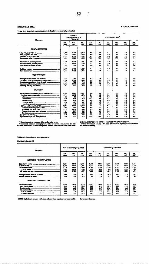
52
HOUSEHOLD DATA
Tobl. A.4. Sde9bd hnclpltyn9nt In.lc0.97, se-son.fly a6usted
HOUSEHOLD DATA
Calegoly 9, '. "
AM99. 64,. Ap'. A4. D-Fl 64,. _1999 1i97 19996 9I 19397 9997 1997 1997
CHARACTERISTIC
T99.1*6 o_ . 72 7,144 6,714 S.5 5.3 .4 9,3 52 49Mm20- 39 9, _.. 3256 3 42 4.4 . 44 4.4 42W6 90 925 0 2Z74 Z771 2.969 4.7 4.9 46 4.7 4.7 4ABa .. 959 Is IS a 1= 304 - .. 2 1229 96. 98. *7.0 7.5 964 9.4
M-W U- p969960990 12937 v.2a 9.161 3.0 3.0 22 2.9 2.8 2.7. m994 p , 1,272°3 9.2C6 1026 2.7 27 933 2. 3.2 3.1
W9.4994 -4. 5_ _ ._ . 992 769 637 7J 64 9., 90 9.1 7.5
Fs6.9 .99969 _. S9579 S7356 5 329 9.4 52 52 9.9 9 .9 * *P9.4.4 0 ..___ _ _ .44 *.428 1.495 5.9 59. 97 6.0 5.7 5.7
OCCUPATION 7
Id..b..94897 o5 M7 2.3 7 4Z Z z9 ZO 2Z0T S 7ml91.99909..994C.v44 9999904669_-....... .750 9.702 ,,53 44 .6 4.4 4* 4* 42P- 19 4 .'At Iw _ 739 732 714 59. 94 SJ 4.7 4.9 420.. 919.081. .9 9296 *.453 72S 7. 72 8.9 89 72F.oA b-y. 09. 9dhq _ _ 303 279 254 7.9 7.7 75 7.5 7.4 65
INDUSTRY
N p9 Ud 99b.9.9 0y _ .. 57905 5.7 447 52 .9 55.4 S.4 5.3 52 9.0G09469's94495~6O.989.8 9.794 9.095 9.579 6.9 5.9 6. 592 5 5 4
6449.90 ~~~ ~~~ ~~~~~~ ~~~ ~~26 29 93 426 7.6 60 4 0 2.0Ca98599,99.......... _- __ 59 674 699 90.3 8.4 909 9.0 98 6.7S498t49 9 ,O3 995 947 4J 4. 4.2 4.5 43 4 4
Dm09.. m.044 979 467 457 4.7 4. 7 4.4 4. 30 2.6N6 IQ.4 . - 427 449 490 59 9.0 42 9J 52 SJ
S--j..9 q kh.s 32.999 . 3.643 ,5S 552 592 52 9.9 49T99999 8- m,.d c94999 296 209 42 0 4. 4.3 4. 228VfCth,." l 01 ____.__. .712 1.675 .69 6.5 652 64 65 63 62
19. h. . 7n 9 . 9 *81 247 255 2.4 2.1 35 2 52 245 _- | .799 9.214 I.522 9.6 52 4.9 5.0 4.
Go-9 99._ _ 545 523 439 .9 2 0 .9 22 28 Z4A94.4-p .96 9 9Y9Z'8 29 22 292 9 9053 6.6 La 9 95
I U-998999999098 06-,490 940d9.59959 99 6990.9 9909.9. - 99949- 50 M690d6.4h 9.9 09998-69--
z 5 KJ tcllK4 ~~~~d"' ID . K 4 NOTE. BepVnh, h1 A.1t 1997. dat rIIK 1 ;Ia= ~dh1 X 1 s~~~~~n, ~4d~ 1 ol Wlo W th. Wboud. W -.
Th966 A.S. tutio. ot un-mployil
Not ..a--09y . dju9SW- So -- lly adj.std
.. . 4-. AV. ' . . Fb. M.. A,.9996 M 997 1997 9899s I99 1987 1997 9997 1997
NUMBER OF UNElltPLOYED
16669989.609 - ~~~~~~ ~~~~2.221 2.313 2.139 2.450 2.671 2.91 2.591 2.650 2.354n s_4. Z3___ 23 2.A63 I2.9 2.332 2397 2253 2.32 2.399 2.956
958 06 90I 2.770 2.423 2439 2397 2179 2155 2.99 2. 2092I I29_. 9.343 1.253 1293 9.9 976 942 9.29 9.329 9.09027. .I 9,Mr36 9427 1.9 947 9299 9.09 9212 9.138 9.98 9.9
Ap 16. 96,3 16,7 1973 99 16.0 I8. 15.3 152n 90.2 6.3 902 as 72 7.7 64 729 63
PERCENT D1STRIEUTION
Tuall fl 11000 10090 109.0 999.9 1012 900.9 900.0 1000 *0101099 9989.009 __h____________________ 59312 319 322 342 37.9 39.0 36.3 37.4 39.799o94. _____________ 29. 99.0 35.2 32.5 32.7 3190 33.4 35.6 32.7
S.9.d o _ 29.8 327 372 3 35.2 302 300 29. 31.79592.299.00 I&II__________ 9 9720 19.7 95.3 932 92. I" 9419 16.02769996 290 19.7 97.5 9. 96.7 96 1I95 992 15.7
0OTE1 9D t9 0 ho0 r9 9. 99.,9.9d9 .h.067

53
HOUSEHOLD DATA
T.ble A4. Region ¶ or unInpiy.-
1,A r h I)
HOUSEHOLD DATA
Not NooOSeNydh
Asn M.r. APo AW. D- J- F. 4.. AIW.1556 i957 ¶907 ¶906 ¶206 ¶067 ¶067 ¶007 1997
NUMBER OF UNEMPLOYED
J.9 ¶01 "90 o 17 - 3.10 3 3.493 3.50 3.W5 3.21 3245 3.163 3.I87 2.79On 0911791017 9309 9,294 1.250 gm9 1.09 997 553 44 1.1 976NO4 rn _010 &) 2.517 U2243 3.9 Z793 2234 2.2 2.21, 2.167 2003p blo10o060916I090 0,299 15° ¶,3 (') (') (~ ) I | ~ V | 69
Job 1. 694 a09 72 723 845 990 797 784 7M4R.060900 ______________________ 30291 2.579 2.0 2.=6497 2.562 2.99 2.649 27535 2.42N909' 53.03 SW9 54 07 M9 900 47 947 M7
PERCENT DISTRIBUTION
Taal 100: 10 o0. loom o0 I oo 110 sa OU 101.0 100 100.0J.b b- " m 0- -00 rd~ M4*6y j9 _ 5097 472 49 4a.3 4.4 4".9 4.7 445 3
nOn bydl 1549. ¶4 16.9 15.1 ¶4.9 ¶3. ¶2 03.9 1¶.3 14.9906¶9119097 rnum 11 -a _ Js 30.3 3Z1 33 909 31.7 0.6 30.3 M9.9
JS9oO¶ .- 9.7 ¶0.0 1.9 99 ¶07 12.3 ¶0.9 I¶1. ¶11R.099,99 06.2 34.2 342 340 3.3 34.6 356. 354 369.
7.4 7.7 92 7. 9.6 9.3 8.9 95 o 86
UNEMPLOYED AS A PERCENT OF THECIVILIAN LABOR FORCE
Jd0 I.- 71 o 4 r_ .. Z7 2.6 2.3 Z6 i4 34 2.3 2.3 2.2.4099400 b .5 A s .5 5 .J .7 .6 .J .J
R _9160610 ¶7 0.0 1.7 1. .99 1.9 3.0 1. 0¶910.9909 .~~~~~~~~~~~~~4 .4 .4 .4 .0 4 .59 .
¶ ¶09600 .ns 01479104999ry.
T.be A-7. R np of afteronatf- m99 of9 r 00d9b041c-I9klon
Not e99009911794009 99990 djoo
_. A. A. D- J- Ap..1999 1997 IM97 1996 ¶I96 ¶007 ¶907 ¶007 1997
U.1 P990 0¶1790 ¶0 _0h o9 b44w. 9p4dftd9 9L3 1.9 1.9 0.9 1.9 J 1.9 1.5 1.5
U-2 .lb bwn 5n r- ,ho _Mfd
999999 Z7 2.9 2.3 2. 2.4 .4 2.3 2.3 2.2
W U4. 79193 n 6 p 4.r9091 d.rn,191 I9b0. ¶ (0dllr I unmdm n s 59 5 0 55 0.3 s4 5.3 52 4.9
U. T799 U pk. ad
961961941109 - 7 5.7 0.1 (I) (V (l( ('1 (¶9 (¶9
U-5 T74 u0OoK Pk. *191d 100 ph. M 611. erTh
U9 10 1 9 8 9.4 9.0 0.9 VIq VI VI V ( '
'c.0-9h.0y9ww- 9.7 9 0 ('I n VI ne s 0' (
NOTE Thb. -9 d ki d lof k w F pl.n a n bf ie " .n Ia. . .n = U l d9 -v41 P 1 90 A-7 4d h9 1994. A9 I97 d .9* p r ID .- 90M1. . 9p961 dd1d L9 F.9m6 9 - P-- 99 -- B- r6. 06.99kdo¶¶i.M - *09.2 kmodoo 91109 ft-009190 .11¶10br16bw h 9199 It" ¶99 01-o..94.t. e -95* 61 l p. - r ¶ 9. 91109 0w 9d 4 .r P.069h.h
_ h ft e PS 0--pd .d- . A- of ,,, l r 097 y J 49 1997. d1ft. 0rdb19.J rp16tb-1-o0,1W .ft h-hk6.

54
HOUSEHOLD DATA
Table A-9. U0emPIOYd P09)990 by S90 and 4g9. seasonally AdC.td
HOUSEHOLD DATA
d pr a , p-
Agp nd (444_)
4-1 40. Ap,. Apl. 999 r.1 e. F~9. Apl.
1999 1997 1991 1996 1996 1997 1997 1997 1997
T91. 16 y097 d 70 7.°2 72144 6.714 5.5 5.3 9.4 5S.3 22 4.9
1619 24 y9 2.93 2.554 2.4.9 11. 11.9 272 12.0 I1.s 11.19141999l. - .5 1.32 Im 19. 19.5 17.0 17. 9,4 1S.41. X _ 621 937 19 190 193 17.7 1 19.4 19.
l1Sa emoco - sO 697 174 152 14.7 1959 *2 1.6 132
2919240 9n 1 359 I2ee 1.2 2 921 29 9. 4 .7 9.0 900
25 4.740 4.191 4326 42 I. 4.0 4.1 4.0 c 67
25. .4. - 25 4.018 3.710 4°4 4 2 42 2 4.1 32
591 0.5 S5W 407 323 2 3.325 3.9 33 32
M191.169919199_9 _ ___ 3 9 9597 7 36.90 9. 9.1 9A 9. 52 4.9
Is 4247019 1.439 .3924 1.331 '2 343 19 2.0 13 1
IS. I-p J.4 1 I7h9 $2
11919979.734 745 701 179 1.97.9 . 17.9 17
1Is.7949.....357 39 350 212 me9 204 'O. 21.4 29.
1 199919...ml. 9 399 36 10-2 19.4 17.1 19.4 157 152
20919249919 999 645 621 92 9.3 92 9.6 0 9.
25 Y199099.... SS7.5 2.999 2.707 4.2 3.8 40 2.9 3.9 2.
251. S. Z.... ~ 7299 2.999 2.993 4.4 . 4.1 4.0 2.9 39
55991144-99273 32 7 21 24 32 2. 2.5 2.
9911119to99191-903 2312 2393S4 3.109 9.4 9.9 53 5S 9.3 429
191924999 ... 1.103 1.170 1.11I9 11I 1. 4 I 11I4 11I.9 II.3 102916191999419... ~~~~~~~~~~~~ 97~~0 583 99 1"2 I5-5 11.5 1S 149 12.9
1 A1-17 2- 299 19.7 19.1 Me 9 197 17 16.5
I9191979Ml9 391 311 255 3193 1994 1 92 19.0 3 113
291249 9 9.4 9.9 9.9 9.9 9.1 92
D _998198l479111....... 2.197 2.202 1.99I 42 42 49. 42 4 3.9
621949-9..9175 1990 1.747' 42 4.7 423 4. 42 3923 I
55P.9Y9 0- 9 p252 227 214 2.6 9 2 2. T2 2.
I q°e l.9111919991 949191011 01994l1 51119 4199119519947999.0 S9
NOTE 8"9 VJ.9.9 y M198719. dU, 9191-94 p01944 19 1911 119d 41
'.b9 Cur9. Pner .... p. I the4 anord 90m d tome -d )9 joho bpl frcuy by9. 0on ... HY4 (5n91d
T9.ed M49. W0. 499 6
99 17 1999 197 1996 1997
NOT IN THE0 LAbOR FORCE
TOWl 11945III 9)19 97.59 67.494 24.56 24. 719 43.064 42.775P1191991191121.41991899(99 5.379 4239 2.255 2.770 2.113 2.716~~~~~~~~~~~~~2. 3113 .76
5.1919-44f1999.~~4.449049419*199.9119l1991
- .~~ 1.59 1.480 749 799 767 79
D CCSC 919 91916917 190c1b411 hbo99l4daf r "11
0904s101 991 c0 91489 493 l 37 27 29 13 1 s73
99491919901899I1114909111909199919
1~~~~~~.113 1.101 479 494 634 See
MULTIPLE J013HOLDERS
T91l1494lj09o419 7-9 72874 4.117 4.123 3.9 2.751Pen1 .19o9048191104Ayd ... .9 9 .1 .1 6.0 9.9 9.3
Pft~~yj~ft~bne____deyob__ft_ 4,250 4.445 2.94 2.631 125S5 12814P1419 (91 -49999 9900 WS, jPb 911 4. I.9 .3 54I5 .19 15
P19904yar47049914977j069b90II4]9118 ~~~~ ~~~241 221 169 162 72 09
99019997799909111971904049911y10b 1.301 1.351~~~~~~~~~~A 796 762 599 590
0919911999911918191918_ 04194 J.9 9191 91149 189 12 11111 14 .4l4h -990 S19 d9l91 o4999 9 -9.&
99191999191919191011919418941949919891911491 111819999119199911,8-7. .0 i9~18 4 64069l9 34 11499919119199~199. 4997 40 -199 19491 119 .hW--
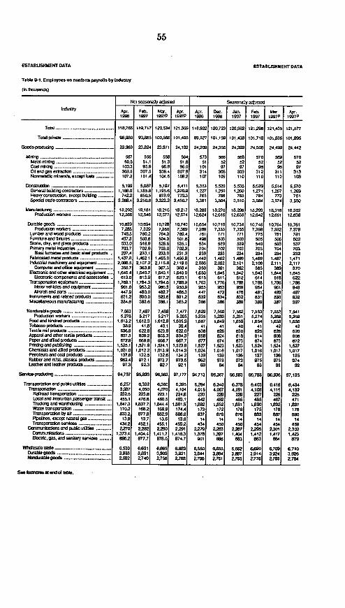
55
ESTABLISHMENT DATA ESTABULiSMENT DATA
T.ble B-1. Eloplyala on no.nto payout by kdwBY
(lo 0S5oducts)
Not soamapi adjusted Seasonomy a5uspstd
v~stry IA S Feb. I 1 I pe. AprI 1 ec. I - I F. lp.l_1993 1997 1997P 1997 [ 19 99 1997 1 1997P J 1997P
TO9 -- --- 118.765 119.717 120.534 121,399 118,922 120.723 120,99 121,399 121.435 121.577
Total pdooe -.----------------- - 98.990 99,995 100.566 101.405 99.527 101.199 101.,438 101.719 101.99 101.995
Goods.71d5c5,Q 22-W 23.824 23,971 24.192 24.20 24,356 24.39 24.509 24.499 24.442
MJdg ...... 567 556 559 564 573 596 569 570 569 570Mo5netal 99.5--------- 51.1 51.3 51.0 SI 52 52 52 52 52
Coal nfrg . ....... 10032 95,9 95,9 99.0 101 97 97 99 99 970Od 5d4asexrati ........ .... . . ..... 399.5 307.5 399.4 307,9 314 308 309 312 311 313N-tloaflfocloeals.excepllofu9 .. 107.2 101.4 104.5 106.2 107 109 110 110 110 199
C0999oU , -i .. 5.199 5.097 5.1917 5.411 5.353 5.520 5.535 SAM3 5.614 5,570Generloibu41drg . ...... ......... .. 1.18560 1.185,8 1.195.6 1.220,9 1.227 1,250 1.250 1.271 1.267 1.259*495Y except9007 building ......... 742.2 650.5 978.9 739.3 765 766 765 764 773 761SpecoialM. c-taroolos 3............ .2. 35.4 3,250,6 3,222 3.450.7 3,361 3.504 3.510 3.554 3.574 3550
Me,,uoacsurng .............. . .... ..... ........ 18.202 15.161 19,216 18.217 18,283 189270 18.96 18.39 19,16 180302Pmouctio1 01519r6. 12.566 12.546 12.577 12.574 12.624 12.616 12.638 12.642 12,651 12.638
Duwobe good . .......... ...................... 10.529 10,694 10.729 1 0.740 10.654 10.710 10.734 10.745 10.764 10.761P1od521920e9;....1..1..9 ... .............. 7,39 7,329 7,390 7,350 7.299 7,33 7.355 7.368 7,30 7.379
Lumber105 a ond. ploducts 748,8 760.2 764.3 76994 761 771 771 775 781 791Fomit. an fixt5ur199............ 497,3 003.6 504.3 501,9 458 503 503 505 5SW 502Sim.. clay. wd 1m p4501duct2........... 533.0 518,9 525.5 525.1 534 529 529 540 538 527Plomary tratl irclu~sts.......... ......... 703.7 702,9 703.0 702. 704 702 752 703 7G4 703
91451101145000591a454 bsi.le rduct0s451 237A 223.1 223.0 221.3 238 223 224 234 224 2322Fobrcated etal0roducs ........ .......... 1.437,9 1.452.1 1,455.0 1.466,9 1.440 1.492 1.499 1.499 1.497 1.471Industrial macnoly " ectoplllea........2.056.5 2.107.2 2.115.8 2.119.0 2.086 2.092 2.101 2.109 2.111 Z.117
Caompltwerud oofce elipou,,o . 356.7 363,9 357.3 355.4 3158 391 352 385 359 370E0e6u6u00and00101, 00915.1 .quiprne 1.645.4 1,940.7 1.60401 1,640.0 1,650 1,945 1,92 1543 1,944 1.645
Eolectoroloooponelos atd acessodel; .. 613.0 613,9 617.2 620.1 615 611 612 614 616 622Tlamspor99ieolleeiuiou ... . .... ... 1.769.1 1.784,3 1,794.6 1.756,9 1,753 1.776 1.756 1.756 1.796 1.799
lubw0,ehicle0s wd0137pmem 9... 61.0 9532, 960.3 950.9 999 952 959 954 991 949Ai-aft Wpanls ..... . ................ 447,9 450.0 492.7 499.3 447 472 476 481 483 497
1mmnrt n d 051l15related p1oduc9s.. 92....... 81.2 920.0 629.6 631.2 832 824 832 831 830 8322M~scellanous nlaruldecdng ......... ........ 384,6 383.6 356.1 305.2 386 399 399 389 387 397
Nondurable goods............... ...... 7.59 7.497 7,488 7.477 7,929 7.560 7.562 7,535 7.552 7.541Pmduction wok04 ..................... 5.278 5.217 52317 5.205 5,335 5.283 5.281 5.274 52359 5.259
F-Id and kir41drod Md.=....... ..... 1,61323 1,912.3 1,1.61 1,95,9 1 ^67 1,949 1.659 1,954 1,55 1.656Tobaoproducts 3. 8.9 41,8 40.1 35.4 41 41 40 41 42 42Textile rnil p10u49 ...............6.......- . 925,9 622.8 622.8 622.0 635 628 630 625 635 620Appoaoel ad oftexl690p0l9ducts 6579 809.2 905.3 804,3 699 824 916 614 905 869Papol and a~lled p71ducts . 9... 72.9 Gags9 96s7 657.7 677 974 673 974 973 672ProdoIv a5d pub5lshin... . .......... ..... . 1,525.1 1.521,9 1,524.1 1,523,8 1,527 1.52 1.52 1.524 1.524 1.527Chemoilds and aoied products........... .1021.0 1.012.2 1.013,9 1.014,3 1.024 1.016 1.017 1.016 1.017 1.017Peroleu s n o~al prducs---------- 137.8 132.5 132.6 134.2 139 139 135 137 135 135RotbbW and11104C. P11SICS Pr54001 .-- 962.4 972.1 673.7 973.5 962 973 972 975 975 974Leal5e a10 le8 he4prducs0.. . .......... 97,3 92.3 927 92.1 56 04 94 93 93 92
Ser,4o.71od. ..... 94.797 95,99 96-59 97.177 94.713 99,39 96,592 96,786 99.98 97.135
Trarlspoelimaond65 public 099509 .... ... .. 6.257 6.332 6,350 6,395 6.294 6,340 6,376 0.403 6.416 6.434Tmosponoadon 3,997 4.050 4.97 4.104 4.015 4.057 4.991 4.105 4.115 4.132
Railrosl Irmspoaooon - -- -. 222.6 223.0 223.1 224.8 233 225 225 227 225 225Local and intewr9a pa0ssenger 0919s.. 450.1 476,9 480.5 492.1 442 492 465 465 497 471Truln5ig a5d irehousing ............... .. 1.847,3 1,937.7 1,844.4 I,951,9 1,952 1 =5 1,961 I.69 1,992 1,567Waler tr0sport8
011 . 170,2 168.2 169.9 174.4 173 172 176 175 175 176
Transportatono by 83................ 93.2 977,9 562.9 856,9 927 979 976 692 567 890Pbpeblnw. excpt ntai gs ..... ..... 13.9 13.7 13.6 13.6 14 14 14 1 4 14 14Traruspoelatiortservices .............. 434.2 452.1 455.1 4S9,2 434 450 450 454 454 459
Coooisraaoroosel and Public odtse 2 I7 2.29 2.290 2.312 .29 2.383 2.7 295 ,31 .302Corrunsoli09ols, .................. . .... 1,373.4 1,404.4 1,411.7 1.416, 1,379 1.39 1.404 1.412 1,417 1.423Elctic. gas. and iloaz Servics ... 9992 977.7 978.0 874.7 901 m8 883 863 864 679-
Whwisale ande 6.530 6,931 6M6 6,9 656.550 555 6.65 6,990 6.709 6.710Durale~ goods ......... ................ . 3.38 3,991 3,9919 3.921 3.864 3.594 3.997 3,914 3,924 3.925N405591109G -- --. .- 2.692 Z.740 2.756 2.5 Z.709 2.761 2.765 2.776 Z.785 2.794
See, o6 o1 mug.
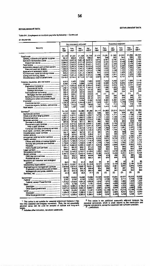
56
ESTABUSWMENT DATA
Table B-1. Emptapses on nonsarm payrols by industry - Continued
(In thnusandsi
Industy
Re ail eade ......... ........................................Builing materials and garden supp5ies.General mrdundidse stores ..................
Depsfrtent stores ....................................Food stores .. .... ._ _ _ .AutOmmoive dealers and service statrs.
New and sed ar dealers .................. ..Apparel and acessory stores .................. .Fumure end home furishings suoresEaing and dinling places .. .......- - -Miscelaneous reta estabishments .............
Finrc. insurancar mnd real estate ----------Fm ram ce .._..................... .................................
Drposi ,rsl .u.. .s .........................Commerciad banks .......... ..Savings institutmins ...............................
Nondrposholy instituions ........................Mortgage batkers and bmklers .............
Secuiry and ooomory bsers ..............Hdding and other inestment of-e ._...
Insurane .............................................
Real estate .... .....................................RealM esm ................................... ............... .
Saervcss2
-. _ ____ .Agnolal" services..... ............. .....Hotels end other bdgig paces ...................Personal servies _ ....... _ ._ _Business services . .. .... ._
Serves to buldings . ...... _Persornnel supply sermices ........................
Help supply servies ....Computer and data processing services..
Auro repair. services. and paring ..............Miscellaneotus repuir services ......................Mollon piFaes ....... ._Amusement od rereation serices ............Health servicnsn . ...... _ .
OAloes and duso d medal dorors.Nursing mid petnald care taciaties..._
Hospilals ...........Horme heath are services _,_.....
l.egl services .........Educaona seri .....................................Social serviAces. .....
Child day wre seis.ces ..._..._.................Rsdnarr..__... ..... ................ ....Resideninal we .---- .....
Museumis mnd boanc arid zoologicgarnbwst..._.__...__..-
Engineenrng and management seroves -_..Engineering and architetural servwmesManagement and pubscrealin ----------
Goviesmnet ....... _._.. ....... .__.. ..... _ _-Federal
Federal. mcept Postat Ser .... .State . .......... __.. _.. .._.
Edutati--on _ --....... -.______Other Srale gcnernnent ........... ..... _._ ...
Local ....................... ...............
Eduction_ ......Oder local govemmenI .... ..........
I rNao seasna7y asshed |
Apr. Feb. Mar Apr.
1996 1997 1997P 19975
21.170 21,401 21 526 21.753go" 992.9 918.6 998.6
2.573.8 2.65738 206.9 2.65752.28423 2.3493 2377n0 2,349.43.3652 3.432,9 3.430.8 3.440,12.24423 2225 2304.5 2.319.1.022.0 1,044,5 1.047.3 1049.81,070.4 1.0,9F9 1,073.7 1.075.5
949.2 1,014.4 1,011.3 1.008897.4493 7.30513 72392.3 7.572.2,616.2 2,739.3 2.712.8 2.710.6
6.912 7.023 7.056 7.086
3.234 3376 3.390 3,4002,014.7 2,030.0 2033.8 2.035.21,450.1 1.478.2 1,481.7 1.4833
2654 253.1 252. 4 251.8505.4 535.9 542.6 4.228.4 243.1 247.3 24.253224 5613 563.6 567.2
241.0 2483 249.6 25122,253 2,2e0 2.264 2.265
1. 46,1 1.545,4 1.5449 1.543.7
706.2 7142 719.3 720.81.365 1.387 1,402 1,421
34,143 34,654 34,988 35290612.3 533.1 564,9 6392
1, 625.1 1 ,622.7 1.639.9 1,6.9,71,2373 1.2642 1,208.3 1.256.5
6.9ss6i 7,229,9 7238.6 7.3762895,8 573,9 877.7 8832
2.0109 2.57523 2.653s9 2.668.12,216,9 2.2623 2.331.7 2I3412
1.170.1 1,21.7 1A07.9 1,319.1,072.2 1,13369 1.143. 1.14.2
3611 363.7 367. 2 371.522.0 533.9 5372 529fl
1,497,9 138123 1.442.4 1,52,9l9,509.4 9,694.9 9,726.9 9I7542
1,6543 1.7083 1,710.4 1,718.1.726,9 1,709. 1,762.9 1,76.13,837,4 388332 3,993.5 3.8972
654.1 661S9 666.1 671.0572,9 94323 949.2 952
2,119,9 2.1483 2,160.1 2,18W2.23972 2.431.7 2,452.4 2485,
585.1 592.1 599.8 600.
.652 676.7 682.0 685.4
822 79.1 81.2 856.t125.1 2. 1301 2141.2 2,1436t.6768 2.970o2 2f992.7 3.024.182.7 654 .8 861. 4 869.881.7 942A4 900.7 9644
45,4 46.0 46.9 471
19785 19.852 19,288 19,9942.767 2,788 2.702 2,760
1,9142 1,848.8 1,851.2 1,852.94 772 4 148 4,7 7 4181
2.0541 2,088 2 .1082 I.11122,6774 2,699 2642 2.69
1. 246 12404 12493 12,4817. 0342 7,165 7 .0 7,195.15,211.4 5238A4 5,265.0 5.2862
-I
ESTABULSHMENT DATA
Apr.
21,415888
2.6752 2068
3,4012,2531,0241,099957
7,46B2.667
6,9423,492.0231.467
265505
(1)534241
2.25l1 .549707
1.7367334,117
6881.8731.173I7,085
2,5692.2721.1691.072
363517
1,5166, 52018.65
I1,72l
31,893661
l I
2.381569861
942.137
834
893(3)
19295l2.776
4.6431.850
22976
6,6825294
Dec.1936
21,931949.7,81
3,461.2.31:
1,044
71,012.75:
32612,49!1.481
25752,
(1)55!241
2.28!1.55*
71.,1,411
621.701,167322
882.6922371.281,12
3753
1,509,671491.763.88
66
94
2.415767
2.81!299
94(3)
19.512,7;
1.814.6,
12,lt
5231
Seasuiia~~~~~~~p started~~~~~~
Seasonasyed~us.id
Jan. Feb.
1997 1997
21.922 21.9406 942 9451 2.736 2.747| 241 2 ,432
; 3.49 3.4722.315 2.322
4 1.047 1.050t 1i1 1.1,0
I 1,017 1.0203 7.571 7,574
22.764 2,757
27.02 7.0771 3.379 3.384l 2.035 2,0371 1.484 1l494
1 255 2001 532 534
(1) (15 560 5645 248 245
5 2.20 2.264i 1. 549 1,549I 711 7151 1,423 1,429
5 35,015 35.10123 634 6382 1,711 1.714
3 1,19 1.1956 7.339 7.4145 878 8850 2,762 2,7329 2.443 2,4032 1 277 1,2916 1.133 1143
0 369 3692 136 5379 .565 1.557
9 9.709 9.72197 1.71 1.7160 1.763 1,76560 3.880 326a6 670 665
3 944 9481 2.016 2.0296 2.425 2.43175 580 58176 678 679
r7 88 87
Z 2.154 2.15ll 2,961 2.9738g 991 997
12 941 949(3) (3)
4 19.544 19.5 l'9 2.725 2,714'0 1360 186642 4.038 4.64
13 1.960 1,870l9 2,676 2,67l53 12e191 12.2151I 6a 6.857IS 5,3#8 5258
Mau,1970
219958
2.7942,4833.47922281,650
1,18
1.0217.5392.770
7,095
3,372,041
1,488253541
568
249
2.021,544
7191,435
35,173631
1,1917.467
893
1207
1,144370525
9.7371.7161,7672.895
667
2.441882694
872.1062.976
ff72952
(3i
1952,
2.708
13s
4,642
2.68012,199
,8,415.35B
Apr.1997P
22.0259642.7802.446
3,480
2.3281,0511,103
1,0197,585
2,788
7,1183,4102.0431,491
252546(l)570251
2.2581. 546
7221,440
35.265632
1 ,7081.1947.486
2.7532Z422
1.3201,149
372528
1,5419.771
1,7231,7722,901
673958
2,0312.453! 94
688
as21573,885
877965
(3)
19,582
Z 27091,8574.693
1.972
12.2208.8r43527
a-22
I This series is no suitable ioc msan, adjuspbent becse it has 3 Tis swies is not puVtsld seaseonaly adjosted bmcase the
very ole. seoA aid iriegular movemeit. Thss. the not Seasonally seamisona c ,npose ehich is sosf relattee to mie send-cyids mid
adjusted sersis cn be used lot anasysi Of cY0al aid bng-terenn bir ar 0 ooponents. cannot be separated wit suffment presbin.tr . ind'stres. m sitose sepsstaly. pnminay."''udd esyoter industries no ls~oan separately.
l -l| s,3n

57
ESTABUSMOENT DATA ESTABUSH4IEW4 DATA
Table B.?. A-119. -eeky bhee . predadl., - ewep.-b~y -erl-e -epr1e eafare payee.f by [.du.",
Industry I -;7-I AP. IFeb
=l,7 tgussed OeSo--4Y e1S~d
I .IA-. I e = 1 Dec. 1 Jan. I e. 1 Mkec. I JAP.99P 49WP 1 1 J9 197
1 199 J937P 937P
To14lyze 6........ .. ........... 34.1 34.5 24A 34.4 34.3 34.A 34.2 34-9 34.A 34.6
Go~-pd-P odU= ............... ........... ....... 40.7 40.7 41.2 41.2 41.0 41.3 40.0 41.3 41.4 41.5
K'16-9 ~~~~~44.0 45.6 45.5 45.0 45.0 45.7 443 48.2 40.1 45.2
C-9reseb60. 38.6 37.4 30.3 38.7 30.0 30.0 37.8 30.0 38.0 30.9
RO~~csn ........... ............ 41.2 41.6 42.0 41.0 41.5 42.0 41.7 41.9 42.1 42.24.2 4.5 4.7 4.6 4.6 4.6 4.7 4.7 4.0 5.0
M.N.kl goeds......... .............. 42.0 42.5 42.0 42.7 42.4 42.7 42.4 42.0 42.0 43.1CKtie61nh=oe ....... 4.5 4.0 5.1 5.0 4.0 4.0 5.0 0.0 5.3 5.4
Lul115P6114W111pyrducts ..... ...... . 40.7 40.2 40.7 41.3 40.0 41.0 40.4 40.0 41.0 41.3Fomso~e 61nd fisu,-e . . 30.7 30.0 30.0 30.5 30.2 40.2 39.7 390A 403 40.2Ste ly n gas oL 43.2 42.0 42.6 42.9 43.4 43.4 42.3 43.5 43.2 43.0Proimay m1etal industries.................436 44.6 44A 44.6 43.0 44.6 44.4 44.7 44.8 40.0Rest l 5,11156,d15 b sic p10M&= - 44.0 44.5 44. 44.2 44.1 44.6 . 44.06M 44.7 44.5Fabricated 111114 plodsL ........ . 41.8 42.2 42.5 42.5 42.3 42.5 42.1 42.5 42.6 43.111145044 aldinely end4 equipnole. ....... 42.7 43.5 43.6 43.6 43.2 43.2 43.1 43.5 43.0 43 .0Elecumi. ant! wh18e, ect,8ieool G o1Moen 40,7 41.7 42.1 41.0 40.0 41.0 41.1 42.1 42.1 42.4TranlsoOnaton ay~pWMr ................ 44.1 44.3 M4A MA6 44A 44.5 45.0 MA 40.1 44.7
Moto' vehi4es 611d qtoip1mem.......... 45.4 * 45.0 45. 43 40.0 45.1 45A9 45.1 45.0 45.4.smleelmso1are1ed prodos .......... 41.3 42.0 42.2 41lA 41.4 42.1 41A6 42.3 42.0 42.1lA-odallenews mamdeclurng ............ . 394 40.1 404 40.2 30.6 40A 40.0 40.7 40.3 40.5
6lord-obe goed ..................... 40.0 40.4 40.7 40.6 40.4 41.0 40A6 40.A 41.0 41.0Mme1111 0O= ............................ 320 4.0 4.2 4.1 4.2 4.3 4.2 4.3 4.4 4.4
Fo~odad kindred predoL,............ .... 40.2 40.7 40.7 40.6 41.1 41.4 41.0 41.3 41.3 41.4T60beCOdO PM ......... ............... 39.4 39.1 30.1 38.7 40.4 41.A 39.4 41.4 39.7 39.3l611e16m114pro1ducs......................40.1 40.3 41.2 41.3 40.3 41A6 41.1 40A6 41.3 41.5AoPP-andi othe0r5 11111l1 prodxLs . .... 36.4 30.0 37.5 37.2 30.5 37.4 37.1 37.1 37A5 37.5PaPar erdafb1e4PdI-etS............. 42.9 43.3 43A6 43.5 43.4 43A8 43.7 43.7 MA. 43.0
Prntn adpoblishg....................37.0 30.1 30A1 38.4 30.1 38.4 30.1 38.5 38.0 30.6Chemicals and1 allied prodeL= .... ...... 42A 43.2 43.2 43.1 42.0 43.0 43.2 43.4 43.2 43.2Patol- ae call p1odoas................. 43.4 43.4 42A8 42.0 (2) (2) (2) (2) (2) (2)Rbb., and nos. plastics prodLsol.........41.1 41.5 41A 41.7 41.4 41.0 41.2 41A6 41.9 42.0L.eathe,ea,14 leather prod, ct.. ............. 37.5 37.0 380A 30.5 37A6 30.0 30.0 30.0 30.8 38.9
S-i4-v0 d.L0 h ......................... 32.4 32.0 32A9 32.7 32.5 33.0 32.4 33.2 33.1 32.
Tnansp~maooand01 pt5k 0100tes...... . . ..... 30.2 39.0 39.0 39.6 30.4 40.0 39.4 40.1 40.2 39.7
Whlesale bade1 ...... ~ 30.1 30.5 38.5 38.3 30.1 30.0 30.0 30A8 30.7 30.3
Ret1116made .1.. ..... ...................... 28.4 2807 23A 28.6 23.6 23A 28.7 20.4 29.2 28.9
Finame. irwrance.a.d realiestale.......... 35.0 36.7 36.0 35.0 (2) (2) (2) (2) (2) (2)
Senoe..... .. m..... 32.2 32.7 32.0 32.4 (2) (2) (2) (2) (2) (2)
1106118. 6114 1641 estat6: ar14 6se866. These g861ps attsm for Irregular onopon~ems. 861186 be separaled .01 su(Oole1ent pr008s1o1.apprownwely4 1611-05115h of1 the 1616 wnp04yees 111 011a611 11611611 p = Prenloimiay.
7 �- =

ESTABUSHMENT DATA
TabIo 8-3. Avrg houdy end weldy *mIndogs of produetlon or noosuper-laoy w.rtskn1
-n prhvate n.onarm payrolls by Industry
Industty
Totel pr,,ate . ............... _Seasonaily atdpsled .... .............
Goodsg .. . ....... .... __ .__.._............... ........Minirng ._.~....__
Cr nstmaittn . _. ..... ____..
Lbrend taon .... ......... ......... ------ __
Duraie goods ......................... ..
Luanbr roe] nood P04655.Furniture end in ures ....................................Stone. dty. end glass products . ..................Prinay metal industries ...............................
Etast lurnaces and batic stnel PoduCts..Fanricrted meut1 products . ....... .........Industrial aneery and eqLiprnt .............Electroni and other electriral equiMent.Transportation eqnypnent ................ ......__
Mblor vehicles and equipme ..................fistrurnents and reiated products _...............Misreelbneous rnanudadtiring ...............
Nonduurttee goods ...........Food end indred products ...........................Tobactn products .......................................Tettile mill products ...................... _Apparel end other tetole products . ..............Paper end allied producrts .............................Printing and publishing .............. ._Chenmials and aelied products ......................Pevoleurn and ceal products ........................Rubber end mis. plastics products ..............Leather end leither products ........................
Stemaice-oducing _._ .................... ............
Transportation end public utgices .......__........
Wholesale pde ..... …... …._.._ ._ ._
Retal trade . ......... ._
Fnance. insurrnce and real estate ._.._.__.. -.
I See tootrrotel.odrie 6-2. P �prelroroary.
58
Average hourty earnings
01e.4 Ma.
ESTABUSHMENT DATA
Average weeldy earnings
Apr.19itf
S11.75
11.72
13235
15.55
15.19
1Z.73
13.2910.33
12.7615.W01 79212.4313.4412.W517527179713.0310.35
11-93
20761657,94
14.6112.5216.171 9.301 1.19
S.41
11i22
14.49
1276
7192
12.76
1.172
S12.1412.10
13.66
16.05
15.65
13.02
13.5810.iO10.34135415 .1017.7812.7213.8912.4117.4317.9613.381057
12.20113418.79999618
14.7912.8916.532.401 1.45
8e2
11.65
14.67
1323
823
13.16
12.25
S12Z1712.15
13.72
16.03
15.64
13.08
13.4106110.4313.0015.1617.712.7513.9412.5017.5418.0813.4610.561226
11.4310.679.916.23
14.9412.9916.4820.4811.50837
11.67
14.68
13.25
826
1322
1229
51r.1 $4000
12.14
13.78
16.18
15.72
13.10
13.6510.6410.4213.0415.1718.02128013.9612.57175518.1313.4510.56
12.a211.4720.52
9.03822
15.0112.9416.49Zo.1311.558.P9
11.5
14.76
13.30
626
13.14
1222
402.00
54335
698.20
586.33
524.48
559.18420.433893255123654.00788.4851857573 .89488.40761.61815.84538.14407.7
47720450.64629.67
386.72939.02629.7747451692.08837.62459.0131538
363.53
558.01
486.16
224.93
45426
37738
A$8rage w42.dy ea0egs
_ Feb. M~~~~~~~~~~~~~~~~~~~~~r.~~~~422.9
555.96
731698
58531
541.63
577.15426.12402 23547068673.46791.21536.7860422517.50772.1580820561.93423336
492.68461.54734.69398.57301.02b40.41491.11714.1088536475.16337.18
323329
593.67
50936
23620
48297
40W.58
S421 .09424.04
56526
72937
590.01
54926
585.16431563416.16553 .0
679.17797.00541.8610.57525.25787.55
282.06558.0142f.62
4986.04t5.20759.1040829308.63651 38504 01'711.94876.54480.70342233
392.04
56426
510.13
237.69
432953
399fiB
$418.99420.04
067.74
728.10
608.36
547.58
562S6439.43411.59659.42676.58795.48544.00608f6i52f.6b762.738212906221424.51
498.57465f68794.12410.11305.76bS2.94496 90709.43b63.59481.6424227
3809i6
564.50
509.39
2t9.1
470.41
395.93
P . pn Sminaty.1 iSee tote 1 W.biB-Z
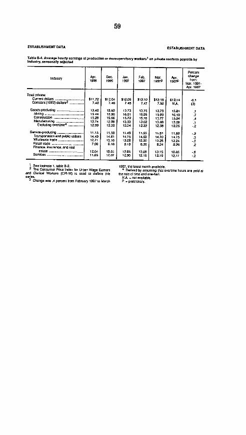
59
ESTABUSHMENT DATA ESTABUSHMENT DATA
Table B-. Average hourty earnings of productlon or nonsupervlsory workers' on private nonarmr payrolls byIndustry, Seasonally adjuste
Percent
Industry Apr. Dec Jan. Feb. Mar. Apr. chang1998 1996 1997 1997 1997P 1997P frormMar. 1967-Apr. 1997
Total private:Currenl do!ars .......................... $11.72 $12.04 $12.05 012.10 $12.15 $12.14 -0.1Conslanl (1982) dolars2 ................ 7.40 7.46 7.46 7.47 7.50 NA (3)
Goods-producing .. ........ 13.40 13.69 13.73 13.75 13.79 13.81 .1Mining .......... . 15.44 15.90 16.01 15.95 15.99 16.10 .7Consructon ...... . 15.66 15.72 15.76 15.77 15.64 .4Manufacturing ....................... 12.74 12.99 13.03 13.02 13.08 13.09 .1
Exclud~ng overtm'e4
................ 12.09 12.30 12.34 12.32 12.38 12.35 -.2
Service-productng ...................... .15 11.50 11.49 11.55 11.61 11.59 -.2Transportatnon and publrc uilies 14.49 14.61 14.75 14.63 14.70 14.75 .3Wholesale trade ....................... 12.71 13.16 13.08 13.20 13.29 13.24 -.3Retail rade .............. ......... 7.90 8.16 8.18 8.20 8.24 8.26 .2Finance. insurance. and real
estate ........... ............ 12.64 13.01 12.95 13.08 13.15 13.05 -.8Services .......... ............. 11.65 12.07 12.06 12.15 12.19 12.17 -.2
1 See bootnole 1. table B-2. 1997. the latest month avadlable.2The Consumer Price Inden for Urban Wage Earners 4 Denved by assuming that overtime hours are paid at
and Clerncal Workes (CPI-W) is used to dellate this he tale of iume and one-hall.senes. NA. oul avaitable.
3Change was .4 percent trom February 1997 to March P . prelimrnary.

60
ESTABUSIIMEhlT DATAESTABUSHMENT DATA
Table B-S. IndeXxs of 9gg9ga.9 weekly hours of poodoUlion or nonsuplrory workrs' on psivl naiodanm payroll by lndlol0y
(1982-100)
Industry
Trotl pr vle ........................ .....
Gowd.Producno ............. . _
Mru ng .- . .... _ _-----__-_._-__
Consiof n ........._.........._ _._.___
Dulraal good .s . ........_ ..... . .._Lumober ad wd products . .................... ..Fumitbe and Gnuns ....................................0t0e. cday, and glass p08ducms ..._..._.........Primary metal Mnustifte ...............................
Bas furnaces and basc stel p sod ..tsFaoricaed metal 0 0oduc0 s . ...........Irdusolial marhinery and equipmnt .............Eec0 aod o0her elerancal equ1pmem1...Twansipwasn e0uip0M ............................
Morte vhicles aod equipmenl . ................tosurrnemos end related podocls ................Misceilaneou nwlaulacluning .......................
Nondurable goods ..........................................Food and kindred produlas . ................._._._Tobar op dxuctS ........................................Tenie mill pzducts . ........... _..Apparel and other tooile products ................Paper and alied plo~dus ................._Printing ald pubishix * ... ....... -Chemicals and allied products ............Pe39leu and ca Products -................. _.Rubber and misc. plastics prrldUcs .._._...._Leath.o a leather produr.s ..................
Serirce-prnducingI .................................................
Toolafsirtatl n od public u0lities ....................
Whldesotrade . ... ..... ............
Retail iando.... ..... ......... ........... ._ _
Fendoe i._su01c. Old l etao _ _
0No seasonally alIbtued
Ap. Fob Ma,. APl.1996 1997 1997P 1997P _
133.6 139.1 137.9 13M1
107.7 106.9
54.2
131.3
105.2
1086132.712.22102.192.671.4
115.5106.1107.81236163274.0
102.0
100.7
03.298.5
107.7121.79B.370SI
141.741.1
149.2
1?9.6
139.0
13Z.5
106.5
179.4
53.7
1402
104.3
106.H132.119 41083290.571.8
112.01025
105.8122.41673729
100.5
100.9107.2
69.775.4
1066122.299.7
73.0138.743.8
145.3
1?5.0
123.1
139.8
123.8
1744
109.0
54.7
137.7
106.5
110.11351125.3105.1
93271.6
116.5107.31 08S.13?5.6167.774.2
103.3
101.610868
59.490B725
15OB.1124.196.671.0
142.94Z.1
150.4
130.4
139.8
133.7
139.5
181.1
110.2
54.7
1462
106.1
109S13892123.6103.1
92.870B
116.8106.910831250163273.3
102.3
100S107.757090.771.7
139.0122.998.472.
142.441.7
150.6
130.5
136.5
13475
181B
APl.
166
135.2
110.0
54.6
146.8
105.7
107.71348120.8108B
91.072.4
113.5103.610b.8
187.472.9
101.4
1029114.164.0
90.175.5
106.512.7100.172.8
139.7439
146.6
127.6
1237
132.7
124.2
175.1
Dec.199P
Soasonedy odjoslod
139.3 137.1 1 140.7 1 140.7
1115
55.1
151.3
106B1
1093137.7125.4110.2
92.672.1
1159
124.0107.9123.
74.2103.8
103.4114.26599Z.173.10B.813.2998
75.5142.643.5
151.7
130.5
127.2
137.1
130.B
181.5
110.5
54.0
147.9
106.1
135.6124.2107.492.272Z8
115.3104.4
105.9126.1167 .7
73.3103.5
102.5113.7
91 .273.1
109.5121.8
98.776.3
140.342.0
149.1
129.
125.4
136.0
12.8
177.7
11Z.6
56.7
156.3
106.9
110.0137.8125.1
111.09298
72.1116.5
103.124.0173.5
74.5
102.0
103.7
114.1
153.8
7327
139.512?32
99.17138
14Z.442.8
153.4
132.3
13?85
139.8
131.1
183.0
112.7
56.8
154.3
107.4
110.5139.8127.01309.493.1
722117.0
106.01 OB9126.7167.5
73.8
103.5
103.1114.262.990972B
110.0124.298.774.1143.5
42.3
153.3
133.0
128.5
1392
131.3
183.0
P . p9rotmiaY.1 See boo ol 1. Nb. B-2.
Apr.
1997P
139.6
113.4
63.7
15Z.3
107.6
110.9140.6
106.793.871.511a8
107.3109.9124.7163.273B.
103.7Im..103 .0
114.2
6Z390.9
72.31309.8
123.499.073.9
143843.4
151.8
131.6
127.1
137.8
1231
181.7
-
_ Il
II
Seas=Cy a4uslad
IiDil
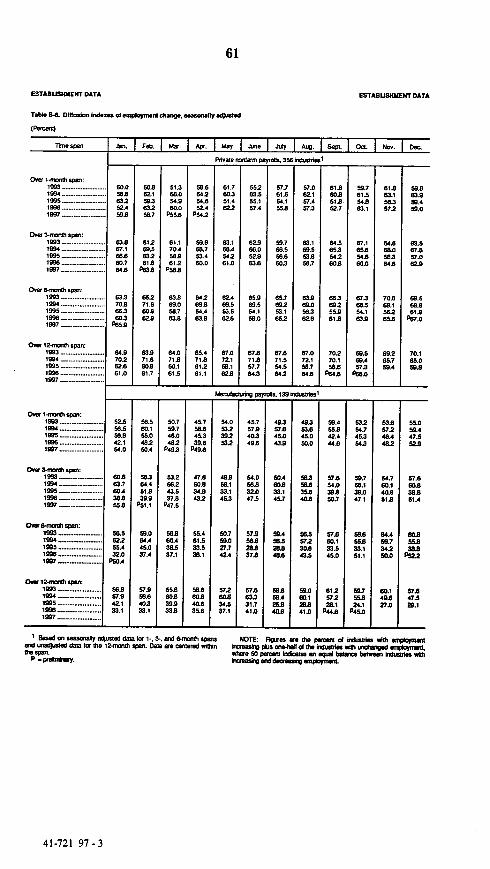
61
ESTABUSS48EPT DATA
Table B.6. DilfflWi Ind 0i ann M dWnga. a y dhrd
(PWW
The span
Om 1.mnhl sa:
1935 .__....._...............1ISS ....... __ .._....
ID37 ......._.._..__......18 3. ..._
1594 __........_.._.
199 7. ..................1934-_5 ..._
lD95 . _ ...... _._.......
1936 _...__......_.......
1 937__....1934 ...... ._
1995 .. _..... ......1936 ._....... ......
085.12.w1560h51p1119931I8 _4..... .
1936718i705....__.__Om 3 rnf sr:
1993
193 .... _..... _...
1993 ..._...1i99731804
Over 6Itthsn
1934
1985 .. ..._...1907 -_ _-
O_ 12.11561 0pan1
1994 _ .._
1937 __.__
J. I Feb.I IM .1 AP. I MayI JOnIJu I A,. IS 1 |e t.-No. |D.c
60.058.863252A
63267.166860.784.8
63J70.8663602
P5S
64.870262n.61.0
52556556642.154.0
60B863.760.4385655.5
62255.432.0
P50A4
56857S42.133.1
60.86Z153J63258.7
612680563261.8
P63fi
65271.860.8632
63S71.860.861.7
565880.155048250.4
58664.451B
582064.4450374
57.S58.S40J33.1
51J68.054D860.0
P55.8
81.170458.8612
P582
63.i
8507
636
64.071.860.1615
50.7S9.746 0482
P49J
532280266 2
43.537B
P47.5
0A4
37.1
552860.8390.332
58.864.254.6524
P542
Gs.753.460.0
64.263.854.4633
65.471.861261.1
45.758B45.339.8
P4 9B
47B860.834.9432
SS461533.538t1
58.660.840.3M6
Pdm. ,rorft payrolls. 356 ianlsi0l
61.780J51.4622
63.166454261.0
62.480 .553.563.8625
67.072.15816328
55263555.157.4
6826025226326
65B69.554.159.0
872712A57.7642
57.761554.1552
53.763556B602
65.763253.1652
67271.5545642
57.06Z.157.4572
63.1635S3BO58.7
90B63.
62B
87072.158 .764B
MW1b80gr Da8rL 139 Mfi d 081
54.0522392532
4865S833.1453
50.7S9.027.742.4
57.2
34537.1
45.757S4023492
54.056S320475
49357245043S
50.460B33.145.7
57,9 1 09AS7S S9u426B 26B837B8 435
57263231.7410
5S259.425i402
4905435Bo450250.0
582
SSBA35B40B.
57230B43.5
59.080.123B410
61B60B851B85Q.7
0425655354260.B
632553961B
70270.1586
P64B
59.4SSB42.444B
57254.036850.7
57260.1332450
6125722B.1
P44B
5S.761.554B63.1
67.165B54260.0
67J
80S
69 .5
54 .16329
69.4573
P68.0
53254.7453543
59.7S13S847.1
5893552,^33.151.1
59.755224.1
P452
61B63.1SS257.2
642tt6.0SuL64B6
70B69.1562852
692
S9.4
53257248A482
54.760.140a512
644
3425020
t0.14ttB270
582S3B58.459.0
03.567257.062S
69.566B
70.1
5.82
55.050.447.5
572aB363
51.4
8025S
522
ass
57.247.8ml.
41-721 97-3
ESTA1U5ISIENT DATA
I M seasonll~y a~u11 dlaim, for1-, 3.. ar08.0618185811pan NOTE: 519ur8s ara the pet8cn 01 inotivtes with emo1mpmr_re w1uwtd dat kw Me 12.05610 &pan Bass ar 1 wIrd on i e=V phus onrtt8I Ot ffxkan id~ Id 81 - OplUo .
81 span. 811 50 P810 clicatus all equal balance Weems 85880885.80P .prsknibwn. klra. end1 daacasi- 81rnplopW8
-
i a
. . . .. . . . . . .
-
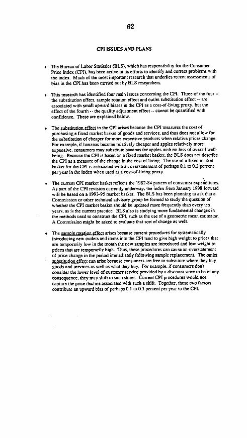
62
CPI ISSUES AND PLANS
* The Bureau of Labor Statistics (BLS), which has responsibility for the ConsumerPrice Index (CPI), has been active in its efforts to identify and correct problems withthe index. Much of the most important research that underlies recent assessments ofbias in the CPI has been carried out by BLS researchers.
* This research has identified four main issues concerning the CPI. Three of the four --the substitution effect, sample rotation effect and outlet substitution effect -- areassociated wish small upward biases in she CPI as a cost-of-living proxy, but theeffect of the fourth -- the quality adjustment effect -- cannot be quantified withconfidence. These are explained below.
* The substtution effect in the CPI arises because the CPI measures the cost ofpurchasing a fixed market basket of goods and services, and thus does not allow forshe substitution of cheaper for more expensive products when relative prices change.For example, if bananas become relatively cheaper and apples relatively moreexpensive, consumers may substitute bananas for apples with no loss of overall well-being. Because the CPI is based on a fixed market basket, the BLS does not describethe CPI as a measure of the change in the cost of living. The use of a fixed marketbasket for the CPI is associated with an overstatement of perhaps 0. to 0.2 percentper year in the index when used as a cost-of-living proxy.
* The current CPI market basket reflects the 1982-84 pattern of consumer expenditures.As part of the CPI revision currently underway, the index from January 1998 forwardwill be based on a 1993-95 market basket. The BLS has been planning to ask that aCommission or other technical advisory group be formed to study she question ofwhether the CPI market basket should be updated more frequently than every tenyears, as is the current practice. BLS also is studying more fundamental changes inthe methods used to construct the CPI, such as the use of a geometric mean estimator.A Commission might be asked to evaluate that sort of change as well.
* The sample rotation effect arises because current procedures for systematicallyintroducing new outlets and items into the CPI tend to give high weight to prices thatare temporarily low in the month the new samples are introduced and low weight toprices that are temporarily high. Thus, these procedures can cause an overstatementof price change in the period immediately following sample replacement. The oletac* bitn deft can arise because consumers are free to substitute where they buygoods and services as well as what they buy. For example, if consumers don'tconsider the lower level of customer service provided by a discount store to be of anyconsequence, they may shift to such stores. Current CPI procedures would notcapture the price decline associated with such a shift. Together, these two factorscontribute an upward bias of perhaps 0.1 to 0.3 percent per year to the CPI.

63
* Having recently established the existence of these latter two effects, the BLS hastaken steps to address the sample rotation problem effective with the data for January1995. If further corrective measures can be identified, they will be incorporated aspart of the ongoing CPI revision and reflected in the data for January 1998 forward.
* Any estimate of overstatement in the CPI as large as 1.5 percent per year requires thatthere be a large osalitv-adiustment bias, arising as a consequence of substantialimprovements in the quality of the goods and services consumers purchase that arenot reflected in the construction of the index. The BLS currently makes aconsiderable effort to properly account for changes in the quality of the items itprices. Although many believe that the CPI is biased upward because qualityimprovements are not fully accounted for, there is little direct evidence to supportthis view. Indeed, some have even suggested that quality adjustment problems leadto a downward, not an upward, bias in the CPI.
* Assessments of the total bias in the CPI as a cost-of-living proxy vary. FederalReserve Board research staff have concluded that the CPI may overstate the changein the cost of living by 0.4 to 1.5 percent per year, though they also say that "theseestimates are by necessity extremely rough." Another review done recently byresearchers at the Congressional Budget Office concludes that the bias in the index isprobably much smaller, in the range from 0.2 to 0.8 percent. Researchers at theDallas Federal Reserve Bank conclude that "a figure of less than I percent ... strikesus as a plausible estimate of the overall [upward) bias" in the CPI, but add "the truefigure may be a lot larger or a lot smaller, at present we simply do not know."
Bureau of Labor StatisticsFebruary 1, 1995

CPI SEMINAR--ATrACMENT 2
CHANGES IN CONSUMER PRICE INDEX COVERAGE AND METHODOLOGYINTRODUCED IN SUCCESSIVE REVISIONS
Expenditure weight Number ofperiod (introduced) areas included
Family characteristics Methodology characteristics
32 Minimum of husband, wife, and one child.Salaried workers must earn less than $2,000 ayear; no limits on wage earners. No slum orcharity families; white only. Resident of U.S.for 5 or more years; no non-English speaking.families
33 Two or more persons. Not more than 2 boarders orlodgers, or guests for more than 26 weeks.Earnings must exceed $300. Salaried workersmust earn less than $2,000. No relief families.White only, except where black population wassignificant part of total; in areas for 9 months ormore.
34 Family income under $10,000 after taxes in surveyyear. No minimum income limit, except that familieswith no income from wage and salary earners wereexcluded. No length of residency, nativity, orracial limitations.
46 Major portion of income of family head must comefrom employment as wage earner or salariedclerical worker.
U.S. city average based onunweighted average of cityindexes, which used regionalweights; no account of areasnot sampled.
Indexes for cities weighted bypopulation in calculation of U.S.City Average. Introduced newitems such as automobiles, radios,and dry cleaning.
Interim adjustment pending com-pletion of 1953 CPI revision. Groupweights were revised to reflect postWW 11 expenditure patterns. Rentindex revised back to 1940 to correctfor "new unit bias".
Expanded item coverage includedowned home-s and restaurant meals.Agsample included small urtnplaces as well as larger cities.
1917-19(1919)
1934-36(1940)
1947-49(1951)
1950(1953)
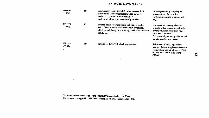
CPI SEMINAR--ATrACMENT 2
56' Single person family included. More than one-halfof combined family income from wage-eamer orworker occupation. A minimum of 37weeks worked for at least one family member.
85 Same as above for wage earner and clerical workerindex. New all urban consumers index introduced,which excluded only rural, military, and institutionalizedpopulation.
852 Same as for 1972-73 for both populations.
Limited probability sampling forselecting items for inclusion.First pricing outside of the centralcity.
Introduced more comprehensiveindex to reflect expenditures for theurban population other than wageand clerical workers.Full probability sampling of items andoutlets was also introduced.
Refinement of rental equivalencemethod of measuring homeownershipcosts, which was introduced in 1983in the CPI-U and in 1985 in theCPI-W.
'Six areas were added in 1966 to the original 50 areas introduced in 1964.2Six areas were dropped in 1988 from the original 91 areas introduced in 1987.
1960-61(1964)
1972-73(1978)
1982-84(1987)

CPI SEMINAR--A1TAQIMENT 3
IIWROVUavS TO TIM CPI DWBur MAJOR ZVZIBZIOS
DATEINPLENENTED
DESCRIPTION
Adjustment of ItemWeights
Interim Market BasketUpdate
New Construction
Quality Adjustment ofNew Automobile Prices
Sample rotation
Rental Equivalence
Return from Sale PriceImputation
Rental Equivalence
Enhanced SeasonalProducts Methodology
Quality Adjustment ofUsed Car Prices
1943
1951
1966
1967
1981
1983
1984
1985
1987
1987
Adjustment of commodity expenditure weightsfor items disappearing from market place.
a. Revised city population weights;b. Correction of new unit bias in rent index;c. Added a number of new products; e.g. TV,
Group Health Insurance Payments;d. Revised commodity weights.
Augmented rent samples with units built after
1960.
New automobile prices adjusted for quality
differences after model change-overs.
Introduced a systematic replacement of
outlets between major revisions.
Changed homeowners' component from cost of
purchase to value of rental services for CPI-U.
Introduced procedure to eliminate downwardbias for items discontinued by outlets that
went out of index with discounted prices.
Changed CPI-W homeowners' component to value
of services.
Enhanced methodology used for seasonal items
by expanding the number of price quotationsto select products from alternate seasons and
eliminate under-representation of such items.
Prices of used cars adjusted for differencesin quality after model change-overs.
CHANGE
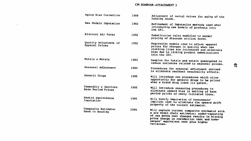
CPI SENUNAR--ATTACHM4ENT 3
Aging Bias Correction
New Models Imputation
Discount Air Fares
Quality Adjustment ofApparel Prices
Hotels & Motels
Seasonal Adjustment
Generic Drugs
Commodity & ServicesBase Period Prices
Rental EquivalenceImputation
Composite EstimatorUsed in Housing
1988
1992
1992
1992
1993
1994
1995
1995
1995
1995
Adjustment of rental values for aging of thehousing stock.
Refinement of imputation methods used whenintroducing new models of products intothe CPI.
Substitution rules modified to permitpricing of discount airline fares.
Regression models used to adjust apparelprices for changes in quality when newclothing lines are introduced and eliminatebias due to linking product substitutionsinto the CPI.
Samples for hotels and motels quadrupled toreduce variances related to seasonal prices.
Procedures for seasonal adjustment revisedto eliminate residual seasonality effects.
Will introduce new procedures which allowopportunity for generic drugs to be pricedwhen a brand drug loses its patent.
Will introduce seasoning procedures toeliminate upward bias in setting of baseperiod prices of newly initiated items.
Will modify imputation of homeowners'implicit rent to eliminate the upward driftproperty of the current estimator.
Will replace current composite estimator witha six month chain estimator; under-reportingof one month rent changes results in missingprice change in residential rent and home-owners' equivalent rent plus highervariances.

68
CPI SEMINAR--A1TACHMENT 4
OWNERS' IMPLICIT RENT
The current Sauerbeck imputation formula for the 6-month owner
relative is (except for a depreciation factor):
I P..Sj =-E p
N ii n i., -a'
where Pi. is the current period pure rent of matched renter i, Pi.. -6 is
the pure rent from 6 months previous, Qj is the set of renters matched
to owner j, and nj is the number of renters in that set. This price
relative is multiplied by the previous owner's implicit rent to arrive at
the new estimated rent.
This imputation formula does not satisfy the "proportionality" principle,
as illustrated by the following example.
Owner implicit Owner implicit
Date Matched rent# I Matched rent # 2 rent: Sauerbeck rent: ratio-of-
formula sums formula
Jan-93 $500 $500 $500 $500
Jul-93 600 500 550 550
Jan-94 600 600 605 600
An alternative formula for the 6-month owner price relative that
satisfies the proportionality criterion is the ratio of sums (A):
E Pi.,* -6,

69
CPI SEMINAR-AITACtMENT 5
ONE- AND SIX-MONTH RENT CHANGES FORSAME-TENANT HOUSING UNITS
CALENDAR YEAR 1993
PANEL NUMBEROF % Mr CHAGES % EXPECTED % REPORTEDHOUSING SINCE LAST RENT CHANGES RENT CHANGES
UNITS COLIECION SIa LASr MON'H SINCE LAST MONTE
All Panels 34,690 30.9 5.1 2.0
Panel 1 5,612 31.0 5.2 2.7(Jan. & July)
Panel 2 5,899 30.3 5.0 2.0(Feb. & Aug.)
Panel 3 5,785 30.8 5.1 1.8(Mar. & Sep.)
Region 4 5,875 30.8 5.1 1.9(Apr. & Oc.)
Region 5 5,973 30.3 5.0 1.9(May & Nov.)
Region 6 5,546 32.2 5.3 1.5(June & Dec.)

70
CPI SEMiNAR-ArrACHMENT 6
Index Estimation for Shelter
The current "composite" estimator for shelter was introduced with twoobjectives: to improve the timeliness of the index and to reduce the
variance. The form of the composite estimator currently used for rent
and homeowners' equivalent rent is
fi=0.65xRzt-ixhT-1 + 0.35xRt.t-6xlt-6,
where It, IL - i, and It - 6 are the current period, previous period, and
period t - 6 indexes for the area, Ri - X is the 1-month relative, which
is calculated using respondent recall of the previous month's rent, andRtt - 6 is the 6-month relative, which is calculated from comparingcurrent rent to the rent reported during the last interview, six monthspreviously.
Because the 6-month relative is considered much more reliable, ingeneral, than the 1-month relative, the following "6-month chained"formula has been studied as an alternative to the current compositeestimator.
It = (Rt, t -6)V16 x It - I
The composite estimation formula for the shelter indexes led tosubstantial variation and oscillating patterns for the index estimatesbecause the 6-month component of the formula produced largeestimates of price change which were applied to a 6-month interval oftime. The 6-month chained formula reduces the overall amount ofvariation by applying a dampened change to a 1-month interval.
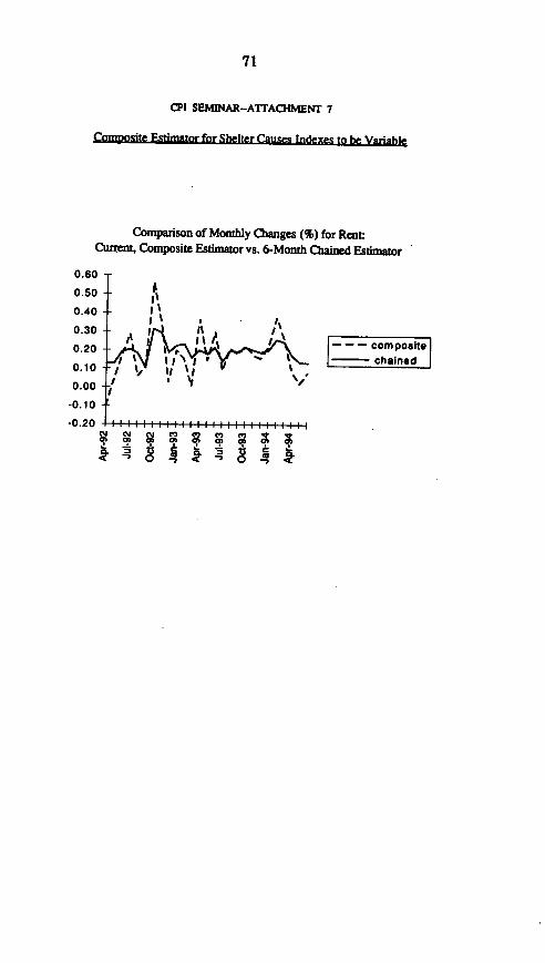
71
CPI SEMINAR-ATTACHMENT 7
ConoAsite Fstimator for Shelter Causes Indexes to be Variable
Comparison of Monthly Changes (%) for Rent:Current, Composite Estimator vs. 6-Month Chained Estimator
0.60
0.50 hi-
0.40 --
0° 20° ark j 1|- Composite0.10 - /,, k t chained|0.00-I \
-0.10
-0.20 - . . . . . .Na N N X X X0V a M a n 0 AE0.C-j .

72
CPI SEMINAR--A1TACHMENT 8
IMPROVING CPI SAMPLE ROTATION PROCEDURESFOR FOOD AT HOME ITEMS
The current procedures assign too much importance to items with temporarily low
prices, and too little to items with temporarily high prices.
Ideally, relative price change in the CPI (Rt,t- I) is a Laspeyres-based estimate
using the ratio of the current cost of purchasing the base period quantities in periodt to the cost in the previous period t-1,
t 1 PtQb
A, Pt - lQb
where P is the price of an item and Qb its base period quantity.
In practice, Point-of-Purchase base period quantities (Qb) are not available; only
estimates of expenditures (EXb) are collected during the base period. Becauseexpenditures are products of quantities and prices, a proxy for base periodquantities can be estimated using the relation Qb = (EXb/Pb), and the Laspeyres-based formula can be re-written as:
, I Pt(EXb / Pb)
R Pt - I (EXb / Pb)
Because the sample is drawn after the base period, the base-period prices (Pb) are
also unknown, and a proxy base price (Pk) for each selected item is calculated by
dividing the link-month price of the item by the price change of the componentitem-area relative from the POPS reference period to the link month, as in
lbPb =-Plink,
Link

73
CPI SEMINAR--ATTACHMENT 8
where lb is the component index value in the POPS base period and 11ink is theindex value at link month.
In the first month after the new sample is introduced, then, the price relative is
R 1 Plink + i(EXb / Pb)Riink +1,ln=
A, Plink(EXb / Pb)
or
_ Ak Plink + I [EXb / (X * Plink)]Rlink + 1, Iin=
A Piink[EXb / (X * Plink)]
where X = lb/Ilink.
In the formula above, there is a negative correlation between the starting price forthe new sample (Plink) and the implicit base period quantity weight[EXb/(X*Plink)]. Thus, the lower the starting (link month) price, the higher theweight of the quote. Because newly sampled items that are on sale or haveunusually low link-month prices tend to increase in price in the next period, theformula has the effect of giving higher weights to items that are increasing in pricethe month after the introduction of the new sample.
For example, in our current procedures, suppose we sample two equally-weightedbananas where the average price in an area is always $2.00, but prices betweenoutlets can vary. In this case, we might have:

74
CPI SEMINAR--ATTACHMENT 8
Base period Link month Link month+1
priceLN price (Plink) price (Plink+11
Banana #1 $2.50 $2.50 $2.00
Banana #2 $1.50 $1.50 $2.00
Since the average price of bananas is assumed to be unchanged over time in our
example, the estimated base period price would be the same as the link month
price. The formula, again, is
Ri Pnk + 1(EXb / Pb)Rlink + I, link =
X, Plink(EXb / Pb)
or, since the expenditures are equal in this example,
+I (Plink + I / Pb)Rlink + 1, link = Pin b
E(Plink / Pb)
Therefore, the estimate of price change in link month +1 would be
(2.00/ 2.50) + (2.00/1.50) = 0.8 +13 = 2.133 = + 6.7 %
(2.50/2.50) + (1.50/1.50) 1 + 1 2
Change in CPI methodology for introducing new samples. Breaking the
correlation between the weight and the starting (link month) price would alleviate
this bias. One way to reduce the correlation would be to price the new sample, and
estimate the base period price for each item in the new sample, some months

75
CPI SEMINAR--ATrACHMENT 8
before actually using the prices for the new sample in index calculation. Duringthis time frame, the old sample would continue to be used in index calculations.Although it is costly to collect prices for both the new and old sample at the sametime, this approach would be of particular benefit for those items where prices arehighly volatile from month to month, such as for most apparel and food items.Indeed, this method is already in place in the CPI for apparel commodities.
Starting in January 1995, BLS will begin pricing both the old and new samples forfood-at-home categories for 3 months. This means that the CPI would continue toprice and use in the index calculation the old samples for food-at-homeobservations for 3 months after the introduction of new food-at-home samples thatwould be priced but not used in index calculations. By doing this, base-periodprices can be calculated that are much less likely to be correlated with price changeafter the new sample is linked into the index. Research indicates that the pricing ofdouble samples for food at home for 3 months will result in the food at home indexincreasing about 0.3-0.4 percent less per year under the new method.
Mathematically, the calculation of the basic item-area price relatives for food athome will then be:
Rink _ _ Plink + I [EXb / (X * Plink - 3)]Rlink + 1, link 1
A, Plink[EXb / (X * Plink - 3)]
where X = lb/Ilink-3.
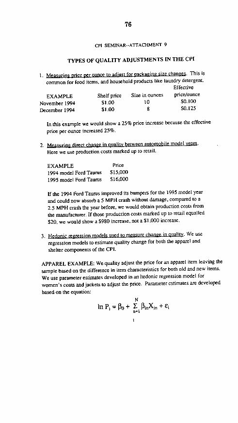
76
CPI SEMINAR--ATr'ACHMENT 9
TYPES OF QUALITY ADJUSTMENTS IN THE CPI
1. Measuring price per ounce to adiust for packaging size changes. This is
common for food items, and household products like laundry detergent.Effective
EXAMPLE Shelf price Size in ounces price/ounce
November 1994 $1.00 10 $0.100
December 1994 $1.00 8 $0.125
In this example we would show a 25% price increase because the effective
price per ounce increased 25%.
2. Measuring direct change in quality between automobile model years.
Here we use production costs marked up to retail.
EXAMPLE Price
1994 model Ford Taurus $15,000
1995 model Ford Taurus $16,000
If the 1994 Ford Taurus improved its bumpers for the 1995 model year
and could now absorb a 5 MPH crash without damage, compared to a
2.5 MPH crash the year before, we would obtain production costs from
the manufacturer. If those production costs marked up to retail equalled
$20, we would show a $980 increase, not a $1,000 increase.
3. Hedonic regression models used to measure change in quality. We use
regression models to estimate quality change for both the apparel and
shelter components of the CPI.
APPAREL EXAMPLE: We quality adjust the price for an apparel item leaving the
sample based on the difference in item characteristics for both old and new items.
We use parameter estimates developed in an hedonic regression model for
women's coats and jackets to adjust the price. Parameter estimates are developed
based on the equation:
N
In Pi = P + I 1inXin + Ein=1

77
CPI SEMINAR--ATTACHMENT 9
Where In Pi represents the natural logarithm of the price of item i, P. is a constant,
Pi. is the parameter estimate developed for the nh characteristic of item i, Xi. is thequantity (or presence or absence) of the nhb characteristic for item i, and e, is arandom disturbance term. The proportional effect of the characteristic'scontribution to price will be exp(p,). In this example, assume only the fibercontent for the new item is different.
Item Description: Old Item Description New Item Description
Design Trenchcoat TrenchcoatFiber All Wool All CottonLength Mid-Calf Mid-CalfLining Full Lining Full Lining
Price Information:
Old Item's Price = $63.00New Item's Price = $40.00Proportional Price Effect for All Wool Characteristic = 0.47896929Proportional Price Effect for All Cotton Characteristic = 0.10039884
Hedonic Quality Adjustment Procedure:
1. Determine All Wool Value to Price (0.47896929)*(63.00) = 30.182. Determine All Cotton Value to Price (0.10039884)*(63.00) = 6.333. Determine the Quality Adjustment Amount (-30.18) + (6.33) = -23.854. Determine Quality Adjusted Price (-23.85) + (63.00) = 39.15
The New Price Change With Quality Adjustment:
Quality-adjusted price change =
[(New Item price/quality-adjusted price of old item)-I] * 100 = 2.2%.
We also use regressions to adjust for the age of the shelter stock.
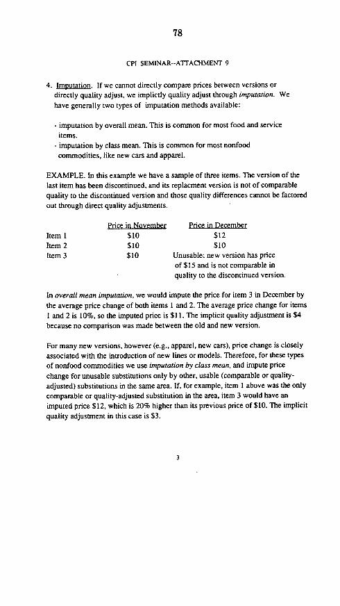
78
CPI SEMINAR--ATrACHMENT 9
4. Imputation. If we cannot directly compare prices between versions ordirectly quality adjust, we implictly quality adjust through imputation. We
have generally two types of imputation methods available:
- imputation by overall mean. This is common for most food and service
items.- imputation by class mean. This is common for most nonfood
commodities, like new cars and apparel.
EXAMPLE. In this example we have a sample of three items. The version of thelast item has been discontinued, and its replacment version is not of comparablequality to the discontinued version and those quality differences cannot be factored
out through direct quality adjustments.
Price in November Price in December
Item 1 $10 $12
Item 2 $10 $10Item 3 $10 Unusable; new version has price
of $15 and is not comparable inquality to the discontinued version.
In overall mean imputation, we would impute the price for item 3 in December by
the average price change of both items I and 2. The average price change for itemsI and 2 is 10%, so the imputed price is $11. The implicit quality adjustment is $4
because no comparison was made between the old and new version.
For many new versions, however (e.g., apparel, new cars), price change is closelyassociated with the introduction of new lines or models. Therefore, for these typesof nonfood commodities we use imputation by class mean, and impute price
change for unusable substitutions only by other, usable (comparable or quality-adjusted) substitutions in the same area. If, for example, item I above was the onlycomparable or quality-adjusted substitution in the area, item 3 would have animputed price $12, which is 20% higher than its previous price of $10. The implicit
quality adjustment in this case is $3.

79
CPI SEMINAR-.ATTACHMENT 10
Problems New Products Pose for the CPH
* Timely introduction of new items
* Whether and how new items should be compared to previous items
* Entirely new items that do not fit in current classification structure
Tvnes of New Products
Renlacement Products -- new models of previously available, but soon to be discontinued,items
May enter through: Substitution, Reinitiation, Sample rotation, Sampleaugmentation, or Major revision
Examples: New automobile models
New season's coats or dresses
Sunnlemental Prduc -- newly added brands or varieties of currently available goods orservices; items with new features
May enter through: Substitution, Reinitiation, Sample rotation, Sampleaugmentation, or Major revision
Examples Generic drugs
Cereal varieties
Special airline ticketfares
Entirely New Products -- not closely tied to any previously available item need a new categoryand therefore must wait for a CPI major revision
May enter only through: Major revision
Examples: Personal computers
Video cameras and recorders

80
CPI SEMINAR--ATrACHMENT 10
How New Items Enter the CPI
Sample rotation
* Regularly scheduled; 20% of sample rotates each year with whole sample rotating over Syears
* New outlet and item samples selected
* New items introduced in proportion to their market share.* New items have no predecessors in the sample; their prices are NOT compared to the
prices of old items.
* Overlapgricing: The market prices of both the old and the new items are collected by thefield representative in month t
Current period price change: AP, = pr - plo
Next period price change: AP,, =1 =P- P
* Assumes quality difference = price difference (between observed market prices of new andold items)
Quality change between items: AQ = Par - p~m
Reinitian
* At the judgment of the National Office, the sample of items in an existing outlet or outktsis re-selected
* Less common.
* Overlap pricing is used in these cases (as above).
* Assumes price difference - quality difference (as above).
2

81
CPI SEMINAR--ATrACHMENT 10
Substtuio
* Usually forced by the marketplace. (Outle permanently discontinues item we havebeen pricing).
* Occasionally directed by the National Office (for example, new car models; genericdrugs).
* Common occurrence, last year, 3.5% of the prices collectedforthe CPI wereforsubstitute items
* No overlap pricing.* Item has a predecessor; price of the new item may be compared to a previous item's
price.* Commodity analyst judges the comparability of the new and old items:
The analyst may deem a newly introduced item to be cmena to is predecessor (essentiallythe same item) (56% of substitutes were deemed comparable.)
Price change between items: A P Pr -P.
Quality change between items: AQ = 0
OR the analyst may decide that is possible to adjust the price of the new item to accountforthe impact of any quality change on its price. (11% of substitutes were in this category.)Price change between items: AP = Pi - P, - QA
Quality change between items: AQ = QA
OR the analyst may declare the new and old items to be nonc pra . Price movement isimputed (set equal to the average pice change of items in its stratum). (33% ofsubstitutes deemed noncomparable.)
Imputation factor: I Avg PI"
Current period price change: AP. = I X PF-T -_
Next period price change: AP,+, = P. -Pl
Quality change between items: AQ = p'-I x pid

82
CPI SEMINAR--ATrACHMENT 10
Sample augmentation
* Triggered by sample shortfall
* Additional items initiated
* Additional items are not compared to previousl priced items; supplement current sample,so there are no previous prices for comparison.
Malor revision
* At approximately 10 year intervals
* New strata and weights
* New base period
* No mapping of old items to new (below stratum level)
* New items introduced with new item strata
4

83
CPI SEMINAR--ATrACHMENT II
EXAMPLE OF NEW PRESCRIPTION DRUG PROCEDURES FORSELECTING BETWEEN BRAND DRUG AND GENERICEQUIVALENT DRUG AFTER THE PATENT EXPIRES.
Tagament - Patent Expired May, 1994. In January 1995, the field staff needsto obtain from the outlet the quantity of prescriptions dispensed for the brandTagament versus the generic equivalent, Cimetidine.
Step I
Item Selection Process -- Probability Proportional to Size
Outlet 1234567 Quote 200
Quantity of PrescriptionsD=ntg dispensed for last 3 months
Running RandomPercent total number
TagamentCimetidineTotal
30150180
17 1-1783 18-100 55
Step 2
A random number between I and 100 was selected from a random numbertable. In this example the selected number was 55 and that number fallswithin the running total for the generic equivalent, Cimetidine. Thus, thegeneric equivalent was selected.
Step 3
The quote described with Cimetidine will be compared to the previousTagament description and any price difference will be reflected in the indexfor January 1995.

84
CPI SEMINAR--ATTACHMENT 12
Example of Laspeyres and geometric mean indexes
The current CPI estimation formula is designed to estimate a Laspeyres
index formula that holds the base-period quantity of an item fixed. The
Laspeyres formula is the ratio of the sum of base-period quantities
times comparison-period prices to the sum of base-period quantities
times base-period prices:
I = Y QoPt' Qo~'o
The geometric mean formula is based on the assumption that a
consumer responds to a I percent price increase by reducing the
quantity purchased by I percent, thus holding the share of total
expenditures on the item fixed. The formula is the product of the ratios
of comparison-period price to base-period price, with each ratio raised
to the power of the base-period expenditure share:
It = rl(p )s where So = Q0PO
The difference between the two formulas can be illustrated by the
following numerical example. Suppose that during the base period the
consumer purchased 5 units of item A, which has a price of $1.00, and
10 units of item B, which has a price of $0.50. During the comparison
period the price of item A and B both increase to $2.00.
Base Period Comrarison Period
Item QuLniti Price Expenditue ndir Share Price
A 5 $1.00 $5.00 0.5 $2.00
B 10 $.50 $5.00 0.5 S2.00

85
CPI SEMINAR--ATrACHMENT 12
The Laspeyres index is
1 5(2)+10(2) 10 + 20 30 3.0005(1) +10(0.5) 5 + 5 10
'Te geometric mean index is
1 =(2)052) = (2)5(4) =(8) =2.828.

86
U. S. Departbment of Labor ComnnissionerBureau of Labor StatisticsWashington, 0.C. 20212
MAY 2 2 W97
Honorable James SaxtonChairman, Joint Economic CommitteeHouse of RepresentativesWashington, D.C. 20515
Dear Congressman Saxton:
At the Joint Economic Committee hearing on May 2, you asked thatI provide you with copies of any written materials pertaining topossible bias in the Consumer Price Index (CPI) that I haddistributed at meetings or otherwise exchanged withAdministration economists.
Based upon my own recollections and a review of my calendar, Ihave been able to identify five meetings at which I, togetherwith other Bureau of Labor Statistics (BLS) staff, briefedAdministration economists on issues pertaining to the CPI. Thefirst of these briefings, organized by the Council of EconomicAdvisers (CRA), was held on December 21, 1994, and was followedby a similar briefing organized by the Office of Management andBudget (OMB), held on January 24, 1995. The written materialsdistributed at these meetings were approximately those includedin the package labeled "Seminar on Current Consumer Price Index(CPI) Issues.' (My staff and I briefed many different groups onCPI issues during the period from December 1994 through March1995, including members of the Board of Governors of the FederalReserve System, Congressional Budget Office staff, andCongressional committee staff; the materials used for thesedifferent briefings were very similar, but we have not retained acopy of a package that can be identified specifically as thatused for either the CBA or the OMB briefing.)
A third briefing, organized by the CBA, was held on March 28,1996; this meeting focused on BLS plans for resolving the so-called "formula bias" problem in the CPI. The announcement ofthose plans, released to the public the next day, is enclosed. Afourth briefing, also organized by the CBA, was held onDecember 10, 1996; that meeting focused on the preliminary BLSreaction to the Final Report of the Advisory Commission to Study

87
Honorable James Saxton--2
MRY 22 KMT
the Consumer Price Index released on December 4, 1996. As best Ican determine, no written materials were distributed at thatsession. Finally, a briefing which focused on BLS plans foraddressing substitution bias in the CPI was held on April 7,1997, again organized by the CRA and again with no writtenmaterials distributed.
Various Administration economists also received copies of thematerials distributed at BLS press briefings held over the pasttwo years on various aspects of the measurement of consumer priceinflation and the construction of the CPI. Five separate pressbriefings were held on the following dates and topics:
(1) February 1, 1995-CPI measurement issues and January 1995CPI improvements.
(2) March 29, 1996--Announcement and explanation of the June andJuly 1996 changes in sample rotation and substitutionprocedures to eliminate 'formula bias.'
(3) December 3, 1996--Background information relevant to theforthcoming Advisory Commission report: the CPI Revisionprocess, the new item structure for 1998, the BLS scannerresearch program, geometric mean issues, the BLS experimentalCPI for the elderly, and other matters.
(4) December 19, 1996--Initial response to the AdvisoryCommissions bias estimates and recommendations.
(5) April 10, 1996-Explanation of the new CPI-U-XG experimentalindex using geometric means.
I would be happy to provide you with copies of any of these pressbriefing packages you would like to have.
Finally, early this month, Janet Yellen, the Chairman of the CEA,wrote to me to ask whether it would be feasible for the BLS toprovide, on an ongoing basis, estimates of the substitution biasin the CPI as a proxy for the cost of living. Her letter to meand my reply are enclosed.
Beyond the written materials I have described and transmitted,there has been considerable informal communication between BLSstaff at all levels and numerous staff, again at all levels, fromother parts of the executive branch. Given the nature of thesecommunications, it would be impossible for me to reconstruct ahistory of them.

88
Honorable James Saxton--3
MKE 22 W
Please let me know if there are any questions about the materialsI have provided.
Sincerely yours,
KATHARINE G. ABRAHAMCommissioner
Enclosures

89
U. S. D*partment of Labor commissione,Bweau of Lator Stat-stcsWashington. 0 C 20212
May 1. 1997
Dr Janet L YellenChairmanCouncil of Economic AdvisersWashington, D.C. 20500
Dear Chairman Yellen:
I am writing in response to the letter I received from you earlier today.
Based upon work the BLS has done and has planned, it would indeed be possible for us toproduce, annually and on an ongoing basis, estimates of the substitution bias in the ConsumerPrice Index (CPI) as used in the tax and benefit indexation formulas cited in your letter. As youare aware, the CPI follows the approach of tracking the price of a fixed market basket of goodsand services. The index therefore does not allow for shifts in consumer purchases in response torelative price change, and, for that reason, provides an upper bound on a true cost-of-living index(COLI).
As your letter indicates, and as I have discussed in recent Congressional hearings, substitution biasmay show up at two levels. The CPI is constructed by first aggregating price quotations to forma series of subindexes for categories of items such as Apples, Men's Shirts, and PrescriptionDrugs, and then aggregating those subindexes to form the overall index. "Lower-level"substitution bias arises because the formula used to aggregate the individual price quotations toform the subindexes does not account for consumers' ability to substitute across items within itemcategories when the relative prices of those items change-for example, when the price ofDelicious apples increases and the price of Granny Smith apples falls. Similarly, the formula usedto aggregate the subindexes to form the overall CPI does not reflect the substitution across itemcategories that takes place when the relative prices of items in different categories change-forexample, when the price of apples falls relative to the price of oranges. This leads to "upper-level" substitution bias.
The experimental "geometric mean" index which the BLS began publishing this month may, undercertain conditions and assumptions, better reflect consumer substitution within CPI itemcategories than the existing measures. Evaluation of the geometric mean formula underlying thenew measure is expected to lead to its partial adoption in the official CPI, which will address thelower-level substitution bias. We will make a decision by the end of this year as to which CPIcategories should employ the geometric mean formula, and we will introduce these modificationsinto the official index, most likely with the release of data for January 1999. We have estimatedthat this will reduce the rate of CPI growth by between zero and one-quarter of one percentagepoint per year, depending on how many, and which, CPI categories are modified to use thegeometric mean approach. Put another way, our current estimate is that lower-level substitution

90
-2-
bias in the CPI is between zero and 0 25 percent per year. By the end of 1997, we expect to havea refined estimate of the lower-level substitution bias in the CPI for the period beginning inJanuary 1995 (or perhaps even earlier), based on our geometric mean research. Accordingly, wewill be able to use these data to estimate the extent of lower-level substitution bias in the CPI asrelevant for the indexation formulas you cite for fiscal year 1999 and thereafter.
With respect to upper-level substitution bias, it is possible to construct a measure that accountsfor substitution across item categories in response to relative price changes, though not on thesame schedule as the current CPI. The expenditure information required to construct such ameasure-one of the so-called superlative indexes-is available only with a lag, so that the indexcannot be produced during the year to which it applies. The BLS cunrently produces suchmeasures on an experimental basis. Based on the historical values of those experimental indexes,our estimates have been that, for periods beginning after the scheduled January 1998 introductionof the updated 1993-1995 market basket, the upper-level substitution bias win averageapproximately 0. 15 percent per year. We expect to be able to provide an updated estimate ofupper-level substitution bias by mid-October of each year, based in part on the previous year'ssuperlative inflation estimate, which should be available at that time. Our Fiscal Year 1998budget submission includes funds to allow us to begin work on construction of a superlative indexof enhanced quality, but such an index could not replace the current CPI due to the lags necessaryfor its computation.
Summing the above estimates, we estimate that the CPI will be subject to an overall substitutionbias of 0.15 to 0.4 percent during 1998. Due to the anticipated incorporation of the geometricmean formula, we would expect the CPI itself to grow between zero and 0.25 percent per yearless rapidly from January 1999 forward than it would have absent this planned change. As thischange will address lower-level substitution bias in the CPI, the estimated average remainingsubstitution bias in the CPI declines to 0.15 percent per year for 1999 and thereafter. Weemphasize that the particular upper-level substitution bias in any one year may vary somewhatfrom this average.
As you know, an updated market basket, reflecting consumer spending patterns in the 1993-1995period, will be introduced into the CPI effective with data for January 1998. Based upon pastexperience with such updatings, along with other evidence, we expect that introduction of thenew market basket will reduce the rate of increase in the index by 0.1 to 0.2 percentage point peryear relative to the current index. For the period prior to January 1998, we estimate that thesubstitution bias in the CPI is higher than the figures cited above for 1998 by a correspondingamount, so that it is in the range from 0.25 to 0.6 percent per year.
Please let me know if I can provide you with any additional information.
Sincerely yours,
Katharine G. AbrahamCommissioner

91
EXECUTIVE OFFICE OF THE PRESIDENTlo w COUNCIL OF ECONOMIC ADVISERS
'X it IWASHINGTON. O.C. stI
THE O WAN May 1, 1997
Dr. Yatharine AbrahamCommisionerBureau of Labor StatisticsDeparm ft of LaborWashington, D.C. 20212
Dear Coaissioner Abraham:
I am writing to aak if the Bureau of Labor Statistics con produce, amnally, on an ongoingbasis, estimates of the extent of substitution bias afiecting the CPI-based indexation formula ofour federal tax and benfit programs.' Such estimates could be used by Congress to correcat forthe substition bias now affecting the COLAs of exing tax benet progams. It would beup to the BLS to determine the appropriate methodology fbr this estimation, taking acount ofany changes that your agency may later implement to offx substitution bis in the ConsumerPrice Index.
As you know, economists are in agreement that the Consuw Price Index ovetaesincreases in the cost of fiving due to a substitution bias that results from the Cr, methodology ofprcing a fixed market basket of goods Because Such a Laspeyres price indet feils to takeaccount of the possibility that buying patterns change when relative prices chge, the CPIrepresents, as you noted in recent testimony, 'an upper bound on the change in the cost of living"
Ongoing research efforts at the BLS have enhanced considerably our knowledge of thelikely mnaitude of substitution bias in the CPI. For eample, the expaimental siqplativeindex that BLS hs been producing provide evidence on the so-called 'upper levelW ubstitutionbias. And the recently announced experimental CPI-U-XG id provides inmght into the likelymaitue of "lower level" substitution bias. I understand that BLS is in the procees of evaluatigwhich CPI basic indexes are best calculated using such eometric n formulas and thatadoption of ouch weighting in some ower level categories ofthe CPI is plamed by Jasnuty 1999.
Would it be possible for BLS, building on this body of reserh to produce technicalestimates of the magntude of substitution bias on a timely and ongoing basis for use in awustingthe indexation of govnment progr currently linked to moven in tbe Ccp7 Suchestimates would facilitate the application of a 'substitution bias adjustment fcto" to the anua
' Ihe indexation formula relevant to taxes in a given caledar year is the increase in theCPI-U for the 12 month period ending in August of the previous year over the prior 12-monthpenod. The indacstion formula relevant to Social Security and a variety of Federal penionprograms is the increae in the CPI-W for the third quarter ofthe previous year over the thirdquarter ofthe prior year.

92
cost-ofliving inreasea of the various Fedenl tax and benet prorams. If it is pouible for BLSto produce such 'substitution bias extirnatca, could you ten me when thes estimates would beavaibc and now provide your best estimate, or range of stimaes, of the maWitude of thesubstitution bias currently enbodied in these CPI-Iinked fonmulas? Could you alo Wd1 whatsteps you are planning to take to address substitution bas directly in the CP, when you plan totake such step and their likely impact on both the CM and also the magnitudc of any remainingsubstitution bias In the indcx?
Estmng the substiution bias in the CPI is an inionta tep in meeting the Criticalobjective of more acouraty meauring changes in the cost of living. I look forward to hearingfrom you
SincM ,
Janet L Yelkn
Dr. Katherine AbrahamCommissionerBureau of Labor StatiuticsDepartment of LaborWashington, DC 20212

93
POR RElAS:E 11.00 AbL E.S.TFlday. Mach 29. 1996
Exlending the Improvemen In CPISample Rotation Procedures andImproving the Procedures forSubstitute Items
Effdctive with the Cons RPie Wd for June 1996, the Bureau of LAbor Statistics will extendto all categories of items in the CPI the change in sample rotnuon procedures inteoduced in theJanuary 1995 CPI for food-at-home categories. In addition, effective with the CPI for July 1996,the BLS will change the way it determines the weight of replacepwent items thai enter the sampleduring certain types of item substitutons. Tese changes will complete die proes of correctinga technical problem that des an item's weight to its expected price change. BLS researchersoriginally identified this problem, nd showed that it can lead to an overstatement of inflaionwhenever new items ae incroduced into the CPI sample, The Senate Finance Conmittee'sAdvisory Commission To Study the CPI has referred to this problem as 'formila bias"
Te simple rotation ImprovementsThe CPI samples items in proportion to consumer expendituses for them. However, as a fixedquantity weight index, the CPI weights items by their quandties. BLS estimates the base periodquantity of a sample item by dividing its base period expenditure by an estimate of its price duningthe same period. BLS estimates the item's base period price by projecting a recent price for theitem back to the base period.
An ardcle ntied "mproving C(P Sample Rotation Procedures" in the October 1994 CPIDeailed Report provides a mathernatical description of how this procedure can lead to 'Yormulabias." The CPI replaces its samples of items and retail outlets on a 5-year rotation to keep themfrom becoming out of dat As part of the sample rotation process, there is an inidation periodduring which BLS staff members find the new outlets and select the items in them. In the overlapperiod, which follows the initiation period, BLS prices both the new and old samples but usesonly the old sample in the cPL The old practice was to estimate the base period prices of theitems in the new sample using their overlap-period prices. Then BLS would also use the overlap-period prices to calculate their subsequent price changes. This double use of the overlap-periodprices can set up a correlation between quantity weight and price change. Relatively highweights were. assigned to items with prices that were temporarily low and therefore rnore likely torise in subsequent periods. Conversely, items with temporarily high prices received relatively lowweighs
Many categores of food itenu exhibit short-term price fluctuations that make it especially likelythat they will suffer from this problem. Effective with the index for January 1995, in a processcalled seasoning," BLS lengthened the overlap period by three months for food-at-home items.The seasoning period isa time to obtain the data needed to properly weight each new sampleobservation before its use in the index. Seasoning breaks the link between the weights for food-at-home items and the prices eventually used in price index calculation. Th CPIDetwiled Reporn
41-721 97 - 4

94
article reemd to above explained this change in the treament of new samples in food-t-home
Starting with the index for June 1996, this teament wL be extended to all other non-sheltercategories in the CPl. atesidential rent and owners' equivalent rent art not subject to "formulabias" and their treatment will not be changed) Prices used in CPI price change calculations willno longer be used also to determine item weights. Item weights for city outlet samples introducedinto the index during 1996 will be based on prices collected during the samples' initiation periods.Subsequent city samples will be handled bV an extension of the 'seasoning" procedure from food-at-home categories to the remainder of the CPL. The overlap period for pricing of both old andnew samples will be lengthened by a mimnurn of three months. Special seasoning or otherprodiedus will be used in several minor sample rotation situations during 1996 and early 1997.
The kem subdftudo proeeWhen an outlet stops selling a CPI sample item, or other circumstances make it necessary ordesirable for the CPI to replace an item it has been following& the CPI field agent finds areplacement item. The object of the substitution process is to find the item in the outlet that ismst simu to the one the CPI had been following. About 3.5 percent of al pricings result insubstitutions. Whenever there is a substitution, a CPl analyst determines if the new item iscompable to. that is, no sigficantly different fom, the item it replaces. If the item is judgedcomparable, there is no break in the series or change in the item's weight About 55 percent ofsubstitutions are comparable. If the substitute is not comparable to the previous item, the analystmay be able to determine the value of the difference and make a quality adjustment to keep theseries continuous. The weight will change according to the value of the quality adjustment, but,since the quality adjustment does not depend on the price of the new item, this will not cause"formula bias." CPI analysts quality-adjust about 15 percent of the substitutions. However,about 30 percent of the substitutes arc neither comparable nor adjustable. In this case, the CPlstart the item's series anew and recalculates its base period price using the price of the substituteitem. As in the sample rotation case, this creates a situation in which the item's weight is notindependent of its probability of price change.
Effective with the CPI for July 1996, the CPI will-except in rare and-extreme cases-no longerrecalculate the base period prce, and hence the implicit quantity weight, of a noncomparablesubstitute item. Instead, the C?! will use tzfe originally calculated weight for the item throughoutthe life of that item series. Thi will prevent "formula bias" from entering the index through itemsubstitution.
Researc on alternative nethbodSince the "formula bias" problem was first identified by BLS researchers, a number of theoreticaland empirical research projects have been conducted to clearly define the problem and evaluate anumber of proposed solutions. The evaluation included simulations of sample rotations usinghistorical data, as well as mathematical derivations. The research indicated that the method ofseasoning, as described above, should effectively eliminate any upward bias associated withestimation of base prices following sample replacement

95
Reast of shmlatiou s nd eeft of Mm CI IBLS analyzed stulados band on two yean of histrical Ql datr to asse the impct of theimprvements to the smxple rtation and item substitution procedures. The u of the
mul tosu t tht th c ombined effect o the two chans wi be to rdc the msuredrate of price change of the all-Iem CP1 by about 0.10 pecent per year. The mehods used in thesimulations aem smii to those that were described in detail in BLS Woking Paper No. 263.lInpments to die Food at Hone, Shelter, and Preactiption Drug Indexes in die U.S.Co r Phc Index
Tbis estmed Impact of 0.10 pecent per year is in addition to the effects od ite auuay 1995chan in rotation procedure for food at hotme. In combination with dmutane improvementsin tde CPI shelter indeXes the 1995 food-at-homre changes were estimated at that time to reducethe raze of gowth in the all-itema index by approximately 0.11 percent per yew.
Because the exact mgnitude of fmrula bis will vary fom year yo yer. the Itmac ofelimiting it hon the index is imposible to calculate precisely in advance Estimed pcentugeeffects on die O mst be based on h ical simultion As tsou permit in dte fiBLS will continue to prepare retospective simulations of tde effects of these and otherMetodooia imptvme
For further information, write to the Bureau of Labor Statistics, Division of Comsune Pu= andPrice Indexes, Room 3615,2 Massachusetts Ave.. NE, Washington, D.C 20212-0001, or call(202) 606-7000.

96
SEMINAR ON CURRENT CONSUMER PRICE INDEX (CPI) ISSUES
List of Attachments
1. Expenditure classes, item strata and entry level items for the CPI and table ofrelative importance of CPI components
2. Changes in Consumer Price Index coverage and methodology introduced insuccessive revisions
3. Improvements to the CPI between major revisions
4. Owners' implicit rent
5. One- and six- month rent changes for same-tenant housing units, calendar year1993
6. Index estimation for shelter
7. Composite estimator for shelter causes indexes to be variable
8. Improving CPI sample rotation procedures for food at home items
9. Types of quality adjustments in the CPI
10. Problems new products pose for the CPI
11. Example of new prescription drug procedures for selecting between branddrug and generic equivalent drug after the patent expires
12. Example of Laspeyres and geometric mean indexes
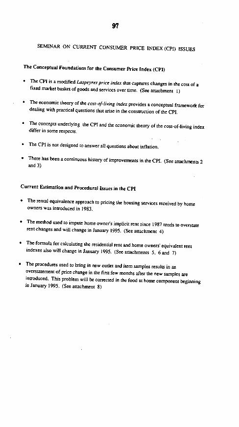
97
SEMINAR ON CURRENT CONSUMER PRICE INDEX (CPI) ISSUES
The Conceptual Foundations for the Consumer Price Index (CPI)
* The CPI is a modified Laspeyres price index that captures changes in the cost of afixed market basket of goods and services over time. (See attachment 1)
* The economic theory of the cost-of-living index provides a conceptual framework fordealing with practical questions that arise in the construction of the CPI.
* The concepts underlying the CPI and the economic theory of the cost-of-living indexdiffer in some respects.
* The CPI is not designed to answer all questions about inflation.
* There has been a continuous history of improvements in the CPI. (See attachments 2and 3)
Current Estimation and Procedural Issues in the CPI
* The rental equivalence approach to pricing the housing services received by homeowners was introduced in 1983.
* The method used to impute home owner's implicit rent since 1987 tends to overstaterent changes and will change in January 1995. (See attachment 4)
* The formula for calculating the residential rent and home owners' equivalent rentindexes also will change in January 1995. (See attachments 5, 6 and 7)
* The procedures used to bring in new outlet and item samples results in anoverstatement of price change in the first few months after the new samples areintroduced. This problem will be corrected in the food at home component beginningin January 1995. (See attachment 8)

98
SEMINAR ON CURRENT CPI ISSUES
Capturing Changes in Quality and Introducing New Goods in the CPI
* Constructing a measure of pure price change requires identifying and excluding the
effect of quality changes in goods and services. (See attachment 9)
* There are a number of areas for which we continue to improve adjustments for quality
changes.
* The total magnitude--and even the direction--of quality change effects on prices not
accounted for by our current procedures is unknown.
* New goods are introduced gradually into the CPI beginning soon after they appear in
the market. (See attachment 10)
* New outlets are also introduced gradually into the CPI.
* Special case: New procedures for introducing generic prescription drugs will take
effect in January 1995. (See attachment I1)
* Medical care pricing continues to be an area of concern.
Market Basket Updating and Imperfect Estimator Issues
* There are limitations to using an index with a fixed market basket as an approximation
to a cost-of-living index.
* BLS plans to update the market basket as part of the CPI revision currently underway.
* BLS continues research on alternative formulas for index aggregation.
* The Geometric mean estimator is an alternative method of estimating price change for
specific goods using expenditure shares for some previous period. (See
attachment 12)
2

99
SENMNAR ON CURRENT CPI ISSUES
Other Issues: CPI for Different Groups in Population
* CPIs are currently available for two population groups.
* At the request of Congress. BLS produces a test index for Older Americans (62 yearsand over).
* Some interest has been expressed in a CPI for the poor.
3
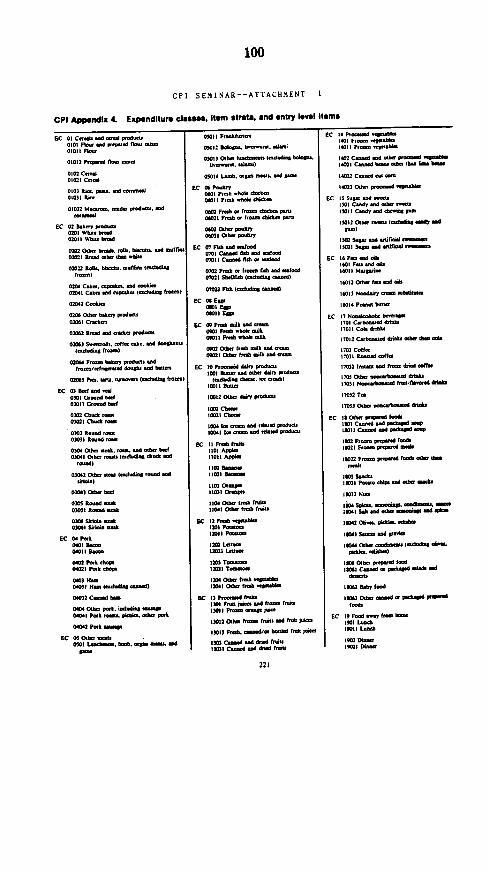
100
CPI SEMINAR--ATTACHMENT I
CPI Appendix 4. Expenditure clases, Item strata, and entry evel Items
EC 09 Cnsb nd 000 nl0190000 .0- pd 0pud 0, 0OIDI I Fb-
01012 ? r-
o0m Cd..0902 C.-10
0903 Ro. P-0 90nm0903 RK.
01032 M000. -J9. pod.u,-0
EC 02 hBkm 01020 .Wb00 b.002011 Wb9 9O9d
mm oa- bf d.a.d b- -Jr_
02ml lld ob. .n i
02022 Rdh. bi9iu 0.m00(0 1Jro)
02m Ck.9. 00n a. eon.Omo Csk. ad -Pk t-hi. I-
02003 Ceolk.
02m0 Obn 99 00009003c02D5I C,.k
02002 iBod 0 0 n. pk.
02063 S5..00. 9ff0 90 10. d .40.b0
OWN Fn bkM VW d
02903 Pi. 90090. 9 1 II
EC 03 Bkd 0190209 GCo.Wd b0030 I G-Gd bd
03m Cbd 00003029 Cba -0
0303 Ro..d 0000003031 R.0d 0
03000O.0=-.0. 000.001909h. 00.00491 Olbn - (.9 d100 60.1b d
01d9
03062 Olb00-a 91.oo 0(_ 0 d
0o3w ad- bfe01901.0903043 0O.00 000
0301 Ro.1 0.
0300004000 0.003061 Su90l00
EC 04 P0kDe01 96.000 01 B-
o002 F0. &qo0ml Poll dlp.
00403 HO.0X I H_ (..d. ..
00032 C..= 0.0
000 0C0= p0. _000 1 -P
0v41 P 0k 0.0= 00- pot
o0o2m = a--
EC 0 Olhn050 L b.b. 900. -M -- 0.0
D1011 000000
0901200 -. Ii .urc 0.9
05013 Olbn b-ks ( bob.L,,l. a-~)
,0504 1b. p. m-0 d
EC 00 00000
0101 FRh wbk h~kka
oom nFfb or frr dwk. oub0009 000 0099 09. 06 P-
ogo] Olhn pOO30031 Olb. P-7
EC 07 Fal0Uh4 .dooo0701 C-od hb old -f00 d0011 C.od 0b r. 0d
Om rn-b .r fo hhb d dooo07m0 Sbl000 (0dW n1.0)
OM2 Fl (crdud -M)
EC 00 E1M|0 ESP
EC 00 00.b 0.l9 .d0nn.000 0. 900.09
WD: 0a0 .9901. 0.996
Mo m lh f-h d ik dn0001 Ob0 F.h nilk 04d0n
EC 90 Pro0190 diY O40d9IWI B.- -d Ob. rI dPr cd
(_Adf d,. Ic. o -
10011 B91
W0912 00. ddr 4roderr
902 Cb_0021 Cb-
;W0Dk -a n d rd nbid pr.d-K10Ds IQ - -o ,1ead pwoue
EC 11 rmb (0009909 ApOI0.99099 AWk.
m2 _
9903 00000099031 Or.Mw
:10$ Oth. fn-h twd10$1 Mdi fnsb Inwu
EC 12 F0.6 ba0.012091000on9209 P.09012011 bulo
93029 0~
1203 T-9031 TAOrrI
0341 000.9 Irnb & n
EC 3 Pr.0d Ihh.9309 0rn n99 0d 190= fr(0901309 P0 ..00M
13012 O (h.9 h-I0 99.0 00.90=
13013 F00. dlor b0090 f(0 j9000
IXI C-w d _lrid fiu301 C3 0 _d dnid In
IC 90 P00000004 .03000000.EC 1. Prow 0-k
1^01 Flo .P-"i1.01 I F-o ,. k
ml1 c bn I- h.c rb h- bI002 C004 .040.0 p.00 o q.9=0 C000 00000000 9
919022 C00001 01
EC 93 S0.w0. 0d9Sol Cu= o0olbn00I 501 I Cad1 -d - P
I5012 Olhn. -09f( S (n _
95021 s d 00il(irl
EC 90 00 04 0b
9 0 01 .. 0
16012 CX-n J.. a-d eb
16013 N-dm -
16014 P-ne b-
EC 17 N... b t1701 Corord dnah1701 I Co.da b
17012 C _-. dnb Zb. lb. d
1707 Celfn17DII Romed -ff-
17032 ID s d f-a driW Wxli
1703 0ln r-b d &kb
17012 T.*
17013 Obn -db. &dxk
EC :9 00- mp. dd9009 C200=W90_ 0 V
'sC: I7 .9.00060 w .00P.000
18021 F- p.P -
9709 Cob 9.09999702 r00.091 9006040.040
97032 90000090=100.090
IsD31 P,-o dip d h- -
19032 N1
1W> Spicn _0 , -_-ISMI Sk d d- -rbn d_
1>42 Cl~ i~l -h"l
1>m} S- usd Pin
J M" Onh n_~ J- dN
:10 lb Id I F
901 099 0 0 019d ..ld -d
dno
110U Orlh. -d n pd Pd
=9.&
EC :9 300d -0 f 1 0
19011 Ie..h
I ml Din
221
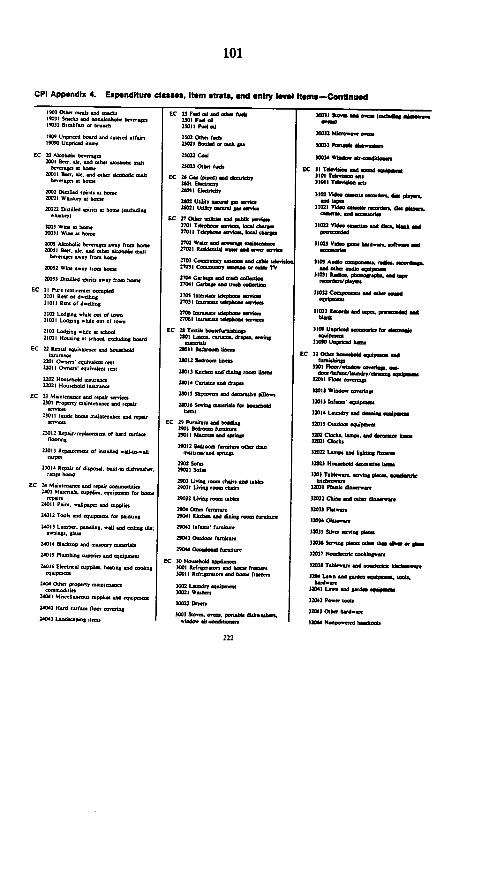
101
CPI Appendix 4. Expenditure classes, Item strata, and entry l1M Items-Continugd
15010 Olbn -n d -k,
29032 81.(o- or brca0b
1909 Uepnod 00d u802, d 6.22..19 Uo.p-d iln0-
EC 20 Akobdic b2.0.2200D Boo- .u d 8. 0dk. 0-h
bvoo,,q.n boo.22023., 0. .0.2.,.02.00.20011 B::. k. ul h.n;e1b.ftor D boo
2002 Drml2. l .l d r ho-
20022 322l6 diil07 . h02 2.0 di
2003 Wm, h-0,0.220D2 Woom bo
200 Akb b-n"n ...y rt b-Q22032 Boo. n k.208 l0n.00.0
b-. .o.y t,0 _ be.
2D532 W2.0 .0y bo- bo
253 D2ia2k0d pdn.- o-y 2,.. 2._..
EC 11 .. _p2 8 d.22 ds2101 R., or dwdhin21011 R., o d0281,8
21022 Lodposg .hik.00 tO22022 L00.2g .h. 02 -ol 0020
210113 2.0O8pg D. 020222.02d2223 Ho..,o 02 0000. 022280 b-d0
EC 22 RnW oror oto b0..0ld
2202 0.o,,, oqotooto nrr22021 On,,o .302020 roo
22r2 H-oth.od 20000022022 Ho-o.ld i000000
EC 23 Mi.Mtn2 Dld reo .i,2302 Prop,,, mo nr0000 0l8 rop.
2W2 2I08. boo, =nio 2 ld ro..
232 0p.lrol ooo 0208.00W12 RM6yir0 Or hvd W-r
23013 RIdnr- or itud0 d .02 -0...oO
2302014 RPor or dl.Pe.9 bi.2.i2 di2h02..
EC 20 Mo tr d uld ropu. _u-rdn2822.002002 PP.002,. 0002000 2. boo
2W002 Pim. o.22p., vd 008,2020
2012 Toold. v0 qWi200 f02. 00200
Wll3 L2.b.. r00i 002 v.08 20020o 0202242.. . o 2
W-14 Blalkp w d~wr nv
2W002 Plb oi. 0p0i0 vd q2p02
Wls6 Eln d ncl ob., b.ra4 vw oolirr
2W00 Oh. ropoy m2e
2040 Moo12o0o. 000020000 vw eqeui
24002 H.d 0200 n00 0,20n0
203 L-d " to,
EC 23 Fed 08 d 000 20b.2300 00808
2302 O2 0 b23021 Bookd n took 300
23022 C.d
2M Orbn (.hd
EC 2ri C 0 028) wd deyh,
2802 Ebe08MUO: I M-kl
2002 Uky o02O, Dn S.28022 Utty 00.0md S.0 -e0J.
EC 27 Obn W-l80 vw rrb.0k -i04272 T _ -- betd dvyr40270o I Tw2.0-0. bd d-
nZM Wn vw -W _d2MD2 ,Rnidm- - vd - -.6
2703 C-rm -y -4 v d 20 b2.27032 Conmfy 0r4 o 000 8 T1V
2Ml I- kpb r4 _ mx2705 o1.- I 8 L 0 00.2
273 I.-00o - -V-27000.0.oo -n
EC 20 Too.2. e..o d-biopWl Li.-c.ir dnpn -J
21o0I B.2wo 2e0,
21012 B0eoo bie.
240103 Kr Oedit eem rE
2401- C-i. vw dnp28020 CS.p- -d d
0..oop,
2W16 SM.4 .-. 0 fo. boedY
EC 29 Frrr- -8 vw.000202901 Weem fr.hru29012 Me w .0r004
2903 Lhie4 oow dr2n v08 0020
29032 Lhbom -. e.h2in
2903~ 1200,. -0 82..00 20029032 ULi. -w 14k.
290. Orho rw-924 ra dw dWMl /e br
M922 InovS fiwlar
23000 Od- f2.0..
EC 30 Hou-roo Hd 002001 JRfim re~ vd -> f-3021 Rdr1r-on vw 0 f0rou
30020 L-.80 em3022 Wvon
2003 30..e. r1ok d8b...
n20
_ 3 10011 200 _d (00.055.i_ 000
Q2<11 Mk- wr10011_ d302300200.., 0
MM340020.. k
EC 11 Td- vd -a nd p-3101 Tdable -431011 Tdo.2o -.n
1101 id.
11022 Vbow - 08000. bFb d
32023 VWO.e0 bdO.-. .0.00 -
3202 Aft2 -p-o. 0.0580. 0020
32021 508WW vw . O
32032 Cop0.. -0 ~d h.--a-M
1109 UWpd-d -l.n f d0.
31090 Ue.Pd 20
EC 32 00. 0..d0 qrdp .d
12dl Fl.. p er
32012 Floe 0 00
32023 Woo.' qp
32022 L 2.0000.20 "0p _
32014 0 v _
3202 CIO.". 0 d02v d0 0 l3203 Ct...
32032 Cteow 20 00U02. r'.oo
12033 H _.8 d00.
120 TvAk- ve. 4rg
203401 2l.. dl
1207 Crb- vw a&nd
3203371 r12MU2 Glo-.v
32037 Sib. iow 2 00
2rIMo Si.4 P.- .1h.4 lb. Oh d S"
32D37 N _od- 088. .
32381.20.., 200 .00w.2 w or41204 LUnn vdD-dl _. kk.-3200 qo 08080 v200..u 0.8.
h2.d.0SM124 L- vw px
12041 Po .08.h
12W24 Olh. hudwv
32030 N2. h.llob

102
CPI AppendIx 4. Expenditure classes, Item trxta. and entry level Items-Continued
p-~bW )30/030 MM 3403404333 UpooW0 33034' .03f333.d 3.0_ 14 m_1_ S~3013 M-"@ ;=k -917 bb'y
1MW - d 36MI FM.'. 0 S U 034.0 d- d bo403.
39090 Uoo'400
3#192 P.Ia b.-V-Wft 36- fO2 M.'. k&-b EC *0 F
d- kP3b9 WU3 134033 M.,m WI M... fl
0340403 0do r 3 30034 M.", O DC I I M.'. (- -
M bdosll p buls aGl lle 36O3S.Mtil' -Ie Wp t sesr AM4 I.0' 3d 30 ' f0.l
330I U34 d _-b.1d l-l 0II.0U 3604 M-o'. .0 AM3 4 - 03..a3 304004 P4.3 03.3a30 3003.4341 M.,. *I.909A=04~ CA .. 3003
3309 U i00 I. M ' . 4il2 Boi' 304v
E0 33 H.d..*"a .Oip60 M30 ', p- -4d .04 *.3 WW', ro_
I S da M Uoon8 .003.pr.d '. olo. d 4.3 EC 401 33.0' -d d4. .
3o01 OM. W.7 d d.1 Ft- m3090 U .4 04103 i.' 33-4. 4 l.4k4' a
3303 HldW PW Woft* i03430 EC 37 lw' . 41012 3I0.04' 4 d3l0 ' ply -d
33033 a300004 M"30. 40- pW- 3703 003.'9303
. b.. C l 3703 I03' D00 1a 4333 33.0'd . dd404 ' 3
33032 9A30. . -3 073 3PB0. git3 37032 DMr F - 41014 I3I,0' .d 3d0 ' _m.0
330# 0OIIY b-..M P_-0
r- 3 37013 07' .3309 43109 UolW 30' Ud0
W3 0
30 wpp3b0 37014 OM' 0d 3. 343 . 0d 30.0
33031 biod 0o3 007 AMUw.,d-
3M332 LO d . d.o WW. 37013 1D ' E C *230.910 m H .0. ha".
4H ' 37016 5,' wl 3,W- 0 0. d 34 3 42033 Fbk f3. 0 ki.0 d. 0 .
30133 P0 37017 Bo7-' . 0 3- 0323030 0 0 d 900.0
34023007034 3709 U., b0,' .f0 d W3 40X3 LU0W
34021 arbydFS - d.WMW3 0007.3408
I~~~~~3M pi I- C 432J.0lb7
MW00.1000390 37090 U-l i03 3C4.04M340 D.004k .O. I 34900303.34301 900000301 13 n EC 33 W.- '- VP-S .3011 W.1b.
340 0333 ba..003d-4 3*33 w n.in.1 4o 4302230.0337
4041 C0.04. d l 8 0 w 33 3 eo 43023 J403437
38 W-'. d3-0
302 W 0 .3 9133 32 0w-.0'. d-in EC 4 Ap 0d -0 i440300.0 aw330 .093
31043 1 Mo0. -- 0. MI 330 433W w_. -* 3. * 3 4011 333 03 l 0 d 033 3n
34044 H.3b3 d L33 3 3.003.04 Wo.-. W W Cm 4012 0033.0 d ppd 304730d
_.t o. 030W1 332 W'. 3 w
i4S C.W3." b04003304d4304740 3 W-', _ .d4 3 3 13 AW3. 0 '0 pW0134
38034 W-,. 0.3i34- *4014 CWAh8 -3
3400 APPi30- 4. f- P0..034063 1 3300303 0. di..4 W .00-d4 30 W -', 8.0 4.3 0 . 44013 W.03 d 3i4033r
*90333.0.0 434M Apwd b.4370d 044d03303
340p10 0 b0d _00 _3 W-', o -30u4 .0 p .. dn0.
3N40290W -'004.0.30 i I A9p333-3 30043 30430300.
74M _r or na ftI,,I wOd .s ec 534003 1.0933030037 03 30003.03 W -'.3 3300.0 EC AS44 303304k0
3407 C- 03 3-4 b4tY. 4d 0'4 Win'. *501 N4 e
343 IC I h .-- 450133 N-
3.071 Cue0 0 d Ol3000dddr, 4d e low45 W-,. &
10 tM b-8051 W-. ., 45M M.t .a.r
3 U I 3.0/40& d bO.b30 Un4P 39w U0 .3d Wo .0i3-033034= N-3a
34003 3 , 3300034d d . 430 4 N-
34I U.3048 ic EC 9 G9 .' EC 46eUd Okk.
ec 33 T ' =I 30 0I Gib' d 4"I3 U3d 033
33011 T n 3102 03i33' d- -03 4W0 AM U0 3 03 30 3 3d
SC 3634M.'. 03 44090 Uov.8. 04h-
XOI M-,.4 ek M104 Glib' -bU e-d *7401 M-li Nsd
XOII1 M... e. 390133003 8.o . 0 47011 M4430 3440
11012 M.'. - -si -ld Ulld pck.b 19016 Oblb' d _ld -- * 707 Ml OD. d1. Ud h. ilel Di
' 223
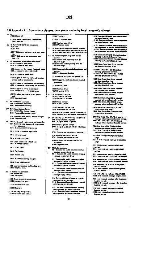
103
CPI Appendix 4. Expenditure classe, Item strata, and entry level Items-Continued
,73I M3406 oll
702 C r0 3 6 6 6. I06 6 6 u4 6mn4d dide
EC 46 A3 . b6 6 3 - l 3 6 d 6 6 -6wOI Tlra"DI I Tira
3602 V06 h 6 6- X6W 60 h-
"MIl V.Wid r ' Xql.PO
EC *7 A3336 b6 6 a6 6 3 - 6 ad 6r 6.701 AU- b dy wort*7011I A.-c:.1e bX7l ort
65023 .66.666636646666.676 r606.6
C u ~ o 60666 r,66 t W tR9 A- a., -k~s-,:
36033 16 .6 . .6 . IQ 6, 6 4. i 6 s
4503 A.Iu66f66. . 3 6 -6 iQ 66ud
4503 IA .3366 .66 6 6 03.6 d66 id.6490. A..-d, po..o 0~ r pu490.I A.-o P-w pi., .P.65033 33: 3ia 666 7 6666e n p66 6u 3490O U.:W 0. 666d 6
EC 50 A7QObilr 6666u6r5003 A -766obil6 i -66u 650 533 A3366 b6b6 i4 6 3 r6
EC S5 V.hid. fuano 63S.3 301 A33 36 obi6 6 ruu- 06. 6606.5101 I A.-: bil, fi- O.nS.
5309 U06 66 6d 6h60 06 d 06. r 6a 7b Sp653050 U:Wp-d n6
EC 52 V6 id,6 6.3. r 666 66. d uX i 63665 30 13 5 66 u 4 1 6 6 6 6 .6 6 6 0b0 4 6 6 6 0 6 6 3 6 0
530133 SI.,6 660376bi366063666060
33032 L-e63 636666b04 666660666
5230) D-. 3. h-
52014 V0 d3 6 i7 763
$207 CtO. -uQobik-.l.e rm33053 A7366604 66bil663
53032 T -kt r66
33033 Pa,036 3rm
7035 3A6. bik 0u 3h06.
20364 0606 6.hid. 7-063.
5309 U:Wk d d46ki6 s ad L. 43 f632 00 U 6
7iad i6606
EC 57 Po l0 k 366676667765303 Ai 6 5W6.
530 3 A u 6 66 66 67 636. 7 6
53023 Olb i3o07 6 T67 6 360S30221 I30 6 06y t- W .0
Si I-doeiy v. W:r.
53022 Sip 3.0
7303 30066 0y U 6wn66 353033 I367666y -p6 7606I6
53032 TvW rv
53033 C. -d - pb
5305066006 .d NW3350) Ualnud -a
EC S. Pr.6.5IV dm rad ad36 pph.-0 P ndrp ed 1dk ppi.
5.03 Pnaivd76 dmaQd aIkwl .,p.
EC 33 No.7wnoivoo dma, vd QdkU
3302 I366 vd -4 76.767066.606.6 dm66
5301 Nonpi W a4.6 _o.
35031 Topo.b vC p
55032 Mdi.4 .6p6 1a p-n W
55033 Sppo6j. d -666r .dierJ
sS71 Hnq. sid,
5350 U.3.6d dmp*505 ULpnad 0666
EC 54 Proaal 66666sos0 Phyb ' 634035 P566666 6656
3602 D-W6 ,-.56023 IDm3 -I
5603 E 7.. vd -156033 Eya36.66 "7r evf
3604 S0sia, by olbn . PrdkaW a,W.[ S-ke by ,h.e adl pf...-b
EC 57 H .pi,.l674.6 .ftd abo 665701 HorpiWol r-0. w-p57033 H6.7.p.J6. i. _
5102 11-7 i.p6 a 05~L HooLi.PW olbn -
SM Nw aM d bo anb
5703 H110i6 o .P.- 657033 1H4.poi,3 -V3.7 -ic
5706 Uncp66d 6 p66 66 676 .dkrlqiw
57050 U7wn.pd 6666
EC 3 6 .H 666i5II3 C.. 6 bah0b _. 66
53113 C W.- bahb _0- I.6 .4
a IP3612 C..0-dd b0hh i_- r.66
56321 C..06666 b000 . 606d4.. 3alap-dd ' .V-
'sI3 C oml66 I 0hb 06 _I36
18111 C l -db66 b br
S$313 C .... ddl 0.3lb _.6 l66d
ami a - -I5lls C..6O66 06.0 _ rruiredw666a,-m an m
56I3 Col 0306._6663_476331 Co666666 066006_66636
5353 a.b 0660066 6666
224
516 Col..0 b06666 1ASW
56136 C.063d6l b0 bl__ n.066.66606wbwft 66
5637 C...." bk6 b6-6 6_
53171 C..6old 0 b -3a.P-d _PJ bJ k _
-l C c e b 6h" m.ami.-pU brfp -V
58161 C...-.W b0.h036 6 6ar666a-6. bop _66.
3821 Ih Crlwoll 91kid4_.... 6a,-6.6.o., d.6766
3mi33h3. C-eu/63b "'W
--W. aPb ' knI56223 63, Cran63 3064 666
M"~ oh. Cmvl. ShW4 rel_am- -i_56223 63.6 C~2o.64366 3646.60
5624 Sb6 Cr1316 Sl66n
58243 6h. Cm63,.b, Shield -66
S32M. Croa1. Shd4 -- n4
51233 S66 C-81B. S0idd .. W
ammp-bosi. rooc7.b -ri56266 3. Crofh.6 6 bbdd64
- Whin-lpil.. -oir38261 366 C-111-b6 Sbidd 6-56664
abe7 11 r C, eql Shd Id
36271 SW C-W6.6 91idd a,..an -. 0b. = bold .I
SM~ Bh. Cro-llh. Shidd f-.WW
3U67 S3W CrB6 Sbidd rn3d
6666666660 36-664l 0.6331 *
ma,06-.66 0.p.6 an0. o
dNP
61-21 -MO rnIw 60*e
36336666 -64 666666.7667Kma
36333 HMO0n4 am p40d _
S3 HM066664 -66666605 m
56343116606663i46666-060666.50
136 00 H60 rnd 066666 _
$831 KMO -U n Pd_h' K_ a
5637 6160 rn-i:6d ami 2166 36l
iSM W ie-a N -w
3636 6606636 .63ai 6666s066 Ha . a63 1-*_6b56o3 6 6"0.606 6660amaW

104
CPI Appendix 4. Expenditure cicss**. Item strata, and entry level Items-Continued
5341 <2.h bnhb --7U ..56621 02202..K 660020020026...0
3662 Oln benhb b0w 20
3662 0266 6020 202260 0000p -pPhy- a
S$43 00.b bfthb o--,r mda00000P0(70000 660,
56621 0220 60026 000000202200
55" (Jlh. h-Rh inrmwl20600402J u00206
SW4 Olnb. hh w nd
$843 O.bn h.h i-pr -~,a. im
56451 OJlh h hb inwn -ndn d.... in a-h. profld7b Yn
394 Ob. bh-fh --7 -g
I oJlb.P n'h w nd
07 Wr h00 hh inmr id-mp-ah np~ia b..PiW -n
7U71 OJb. bg'h -c~ rndn
W.W .Olhn benbi-w i nd
5M M.im h.yad-.
366 026h6 h.2.lh in ndred0.006 -.P.-00 bo0pi6 d -
EC Yl Rding mml
77071 020Nw.m 262062006
$902 lml.S p00c0Ir00d blolu
"286 02k6 pb.1h20d h006 bk dubr
006B0-6 aa p.20 2d 006 b6
79W Unpew n_llmn"M0 Upid i r
EC 60 Sp 6.2 2 4nd0_nGODl Spau hon. mredinbseIOwl I (Jlb-nd -so Ud pn.d M-a
50012 U02.0 d b00 02 .02
6002100d-02600-b20 .. 60 M
W- ml~slm-eil.n m-
5662 H026 NM22 0 d _062
00208.02P20 iaam 6200
EC 39 Tv. h.bbi. nd aW _
6101 Top. bobb. d awx _k6 Oil Tep. S-, ud bobbW.
36102 P06. K9 Pn
41013 hlw iwu A
6102 Pba.aVtX pp00 -d q0 621061 R0
560= P00610hk -02d0601PU6
10 110064 62026
PC 60 SP-0 6000000P2020d 061021 P02. r-d10 .2020 000
02032 P06 of PM0P. 6 p v vP
61091 U.pri0d W. 0262006. i003000
61M> Unpild N-s
EC 62 E D-,,,, -6201 0.6 -bmhp d0a ,,d f-r620221 Clb v m2b-iv d0- 2660
620 F0 f2. 50 pip62021 00 f0 vP-.. P-.
62032 2A06.022 -- 2 fo .604
62032 Ad6is. 006 00200 v0
62 F.. fo. nons or .br m62062 Fe- f2. la 0 r b
6203 PObo..Pwo . ft p600020 PV
620320 60.0602o f6
62032 FR. p0O.(0i0
62053 P. o
62034 V -~h~ 6
62055 O mon .0.soao
6209 U11 ed r0.2 Of ;0001
62700 U0pd06d 6660
EC 63 Tobo- vodw6302 b 1 d.206 000606 020020
6301 0 0C00263022 Tobo- po40, 0262 6.
63013 SOkj. -0
6329 U1pnod ko podw
EC 66 g000 e6 vpv- w
6601 H&. d0.l. .,f6. D.101pn.onW -, p2ld4I
6.011 FPod6 .00 W. b06
6.012 Nok-1 anid fo. lbihMi,
66013 wo-',, b2i. pk .- l
6W" DQ.. Vd. X.d do
6 015 Sb.64. .0 v o. 0 -.
66016 D06 02,002
-P-...o6.yP.0060 p~oo0
66027 El022 p dO~ 020 Vo
660 Coono0/oO06 p0p0lliO0 .6
66031 C-.020 b.W./2k-P- -d _0
EC 63 P-ona -. .6501 BcY pclol -w r.fD65011 11Y p.0 -i fo fow
6302 H5.U.o Pld ob b2v ho
6X17 H&-u ad ol.e b.b "hP6000 aol.
650 UpnPad nW1i -f pd.-W
6SM U.pe-d hn-
PC 666060.6 book. .64 apo6aEC 66 SC'"o b-k. nd V vpl_
6601 Sh60 btk. nd .oppL. f.
66022 C022. 2-ba-6.
602 Rd-.0 book. .64 da.lu4n high hbaS bk.t
66021 El68 0 0 WA hbkb-k, vd VPv'Ua
66022 EP2yd0pdid nd lb.- *r006k.d b.k.o
602 U.pn 0 d .. 4 2 6bod
66W0 Unad il-k
EC 67 D.70t2 2222200.d .h. ellodP66-
6701 C0026 20l00 .6vd P067011 CoO.06 l 0.64 nd f60
6702 E2660l02' 0d 60hy b.6
670221 El-on .n h6 d60-iun d f.,d f_-
6703 Child doyon. o..rY 6..067031 Dnyo.o. nd ooro0Y d
6700 I TV 0d .64 2067042 T,6.hi.64 60-00.600
l1.i nd fuld f
6700 U1p104d a04d2620 nbod00200. D.06 .0nnd abn
67031 Un.vnu 0600
EC 66 L.00 finlall. nd fP L
68011 L000 Pm
610 Bnkin 4Od mn74 P_61021 Sf.P 0.p32i0 b.o -
68022 C6ki.0 -00 0 d q6
60023 T.u .-. 60 P.0d ndabo n.ung (m
6603 C-662y lou -d f0-6
68031 F-. mlcpnu
61000 Cvmo0 22 nd anu
69w Upw-d .ilU- P---
6wo Unpkwe i-
EC 69 i2d2000 P,-.- 6 _6701 Id -t r
qw-
69012 C,0600 006 0d
60023 T700 . peipbnL
66020 C0.26 600ddI20 _.62-nd yp-o
60015 M0 i6f0 pw;ip Vn
EC 72 W2illy 0 pn0 n7260 UlifilY -W;r y.. 40 ub7260112 U02000 - 0. 602402.0
7261 U11221 -Wo2 S 100. 2072611 Ulilbw 300S62202 100 Mt
7262 E2ncit6. 700 ki026u b60
225
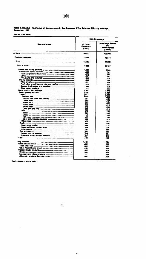
105
Tfbb 1. Roan hIoporlac ofr comcai5nb An tos Conseaive Pride kdxoa UAL dly ,
(p- com d dC _ -)
UA CR A"ft
nem Wad W" Al u~s urb We Eanrc4mlnr alda
Al 4556 _ ...... 0. - __000 _ ICO.A
FCoo ad bo_.u .MM 19___ ___.. 17291 34
Food _ - - 15.9 1 782=
FPoo at h W._ .............. _.__............ 11.187
Cam. VW baery P.__ 1.464 IeeoCerel Md off" -_ ..O.. .448 .541
FbV Old PVgpwd Isa l _ _. .072 M5Co. _ _ _ 097 341Rio. p&M. old amno~W~l .110
OMMuYPMM .d 1.119Whit bm -41 2seFresh OMe bbamf mk and oodie - 2n Z3C-*bakXd*_............. _el ___. _1l am .... ~. .360. AUSs00. polft NW . _- Om 3A1
MM%.. Palley. erl 45 h 2A26 3.2m __....... _.... 2....... 51435
9.el aM ~~~~~~~~~sd ~ ~ ~ ~ 1.529~~IA 1.249GoMbeed 06,. ma ma l .451C sMM ._ ....................... __ _1........ ... 507
oural MM . .... ..... ........................... __ __ __ - .36 4_1Rourd lan .....___._.___...... .. ....... AM e JOlSPut . Stsh . ....... . .. ..... .072 704Ote boa ad _ts ......... __ ._........ MI .41e0^lPaoko. A". .6 .706chops __-----_----_----.147 .1_.Kmo . .15_ .1_6Ot hr N _r--- .199 245
Cv, m B . .. . .......... .................. 46 .4G821aley .__. _ _._._............ _.___. ........ __.. ..442 .4956Fnd whl4 chicken .. ... ........ ...- .145 .173Flmh and tnol ceheck pw) ._ .... ............ .210 .22O rw paary .. .... __._._._...__.___.._......... .. . .oe6
Flh an mood _ 170 1 97Casnd fth ar.aldood An. . .064FP1h bow 1 o ....anal _ _ .5z fi4 .313
Eg . -_.. . _. . _ . _ . . ........... _15 .156
Daily VdC ___ .... . ...........1_91 1.321FnFsh met a~nb __ __ ._-------- -_---- .........,, . . . ... 43 .707
Frnsh - n _ .k 349 .435OOwb.yh r 1n .a ...... Ms.l .271
POW da i d4ply 0, I ......k W e.0..............40. . _ _ .019
S_. hOD el and t.t.
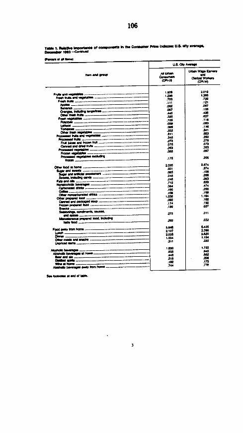
106
TgW 1. fq hiipM . oef _ ' 0I C-llS PlP blbxC t U.L "ty t * -
O0asrowt 1d -C
no.m No pou
Fnu^ _d .09 tf f . ..................... ._.__...__._ ._._Fm0 *4r d _ ... ___..--- ---
-mv - -0
COWe *So -po
F fr._____________d
Fruin4M W .___._--..
Tr p -- ___Rome -f w
FoN food at l -__
sum _6Nm, ------------qSmgo -oc -Sam st WC&#ig.
Pal ad _ e
reh bd Mke 1 .____..___Cow - d _ ._.._.-_.
Ra F s4 -_._ ---- -s ----
8n ck _ _ _ _ . ........C5 dW-- ----
_- - boLha
Food eary __ _m
Owes ne St-
tboo . __o. _gi_ _ 0 1..- _
aad am0 _ _Ale _1 B h_.._
Aom bewau ay amml06 - SI 6.401*1Aloaft g wyer o
See sp l at ad _ _ _ _ _.le
u--~~~~~~~~~~~~~~~~~~.S ~ WqUA at Amv
AS MM Wa W0EMM
.703 .706
.111 1l21
.062 .oer
.0C7 w 1 '
.443 .43
.505 . 62e7
.100 .110
.050 Ie=
.000 .116
.611 .663
Im 270.076 .0on
ca0 .067
.17 206
2320 2.674m33l 74.0xs .10l.248 20
246 263.712 .032J64 .474.100 206.120 .ASO
1030 1.104.002 .102174 .162
m7 .311
.262 .523
2107 213
52.22 5.201.04 1.104Jlla m
.96 .043Jil 2=.446 m.216 .206.192 .173.744 .77?
3

107
Table 1. Relaive I go tovc of compionml is UI Cornemmwr Prille. sieect.1A11Ltly-yine.December 11183 --Cm..,,.
(Peows Of di 868.a)
"COt ...................... ...... .........~...
R&M .~ h .Nag ....................------- -
Mlem cam t
... ... .... ..
Ma~Wm VWd 18Wei
(W'8.548 8698.1W0141-4odiga
N 8wo W8m atDMbe ...... .....o.06 ._........
NO ol ...a. ..... ay (n0. S )...
08w 081868 mnd p4886 IeMm.. .
50a8IdtS~~~~~~~~~548 ..................
TmOElh~etrcit al-......................... . ...
dw (omgm ........ ..... ............ -...TWPPM8 M . .... .............. ........
Loca 8 ru gas............. .............. .......... .-11't we- f ............... .- ..........VWale aMd mdmra omars .............. ....
H .s~j,dO W U ........ . .... . .. ....4..................
1'O~rg a,.* 8s.g ..... 0480148816.
aM p."imis l l................. ......... . .. ..408 dac wucaM 861 oNW) o. ...a...... ........ ......
86 1088168D 84ck s ........ ..................... .
U.& City AnWu
Al O Us be Wag. Ear..,r
(CPHJ Clft Watkir
27.84879ad8.7712.213
.220
19.768
.078
026.042
3.883
256.118
3.814i.'4381.175
1.7481.184
.352242.782.561.217
8.18334601.372
.382.211.183.30.88481
.080
280.300.911.088
.178238.213.187
.32
.70.814
38.814
81.088
1.487
1.324.W8
1.074
.324
.118
3.047
2.001
.220
.2473.8420
.2178.800
.317
3425
4202
.1782868948.531.ISO
.247
.332
.101.111.120
1.72
I.23
.079
4

108
Tom 1. Rpamve wnprmatCS of @flwofl 1In Vw Co w PF x 1nd0x5 U. Cft aVem,Deownbsr 1903 - t
(P.im at A 1ol
n1.a m e sm
La-by a W4 rn d - V . e-X I, .o ............ ......................
Lm40 m - ~-~ - w-as ~- -Hmnaat444 - - t a.y ....... ........... ......._
Gq h .W O W lt| W d _00 WA_ ................... .................._____
PO M -w __ -- ------- ...................... ___..... _._.._..... _.._ ._............_.__GAr4IW maW kcft lePai-a -----0 --- ------
G&den"o wW -V hmaad - oBobo -k----------m ~ e at . .......Cl h ,rd . . ..... . .. ........... .......... .......____ _
U4 __.._____...__-_Co A W " O___ v. 4w-m f..... ........ ......... .................. _. .. .__.
Ap a w . ................ ............. __._.__..... . .__... ......
Apwo _. ,. .. .i_ ko,,,.,,.......... ..... ............................
k$n s ........ .. .................. ___.__............._____....._._48m uft =0S 0.106 ... .......
Fw xnp ad MW CM ....... - -. --_._-----
5h % . - ..os ........ .............. ... ......Mul ft e .... .........
..l..._....._........... ................. ............... .......... ....... .......
D. a ......... ... .... ............. ..._. _._................ -__._---
ae, . _00 _a m.. m_ .- _.
ww 'an.n 0% _ ._ ............... ...... . _._.__ ........ _.._.__..._._._ ..... ......
Fw.e'0 and s_08 do..........______ . ____
nd W --_- -............. ------- -- --- _- ---------
U_. d._. rmWonUwW *koft4
nd _ _ ............... .... . ..............__ ._.. ____UspuW ___.____._ . ...... .......
40 w0 mcceem*diu - ----- ---------- -----w _. _ . ................... _._ .... _.__....... ___ ....._
Gnw - ~.. .......... .......... ......Wa........... .. .... ........................ ................ .......... ..... ...
cqS co O m^ . r .................... ............ ....... __ .......... _.a ....................... .... ... ...........
Wald I . . ............... ..................
Jr V y . ......... .. . .. _.___ ......... .................. _.._....
Fo"t . . ......... _.,_ ... _____..... ...... -__,,,._____-Mule
o O.s - - - .........__ ._.__ .. . .__ ........___..__
AM " s r -d ----- _ . _ .. ................. ...________
LON40Y OM dmY dem. OdW VWlen a__MId ... .......... ................................... _ _ .._1o _p o e O .._ .. . .. . .... ..............._.__....___.... .. ._._..._._._.-_
S foW at VW al .
U.S. Cty A.p
MLSAXI Up Wae Em
c4ar waoflC0105*llmW a.(Cl W)lu
1.109
.359
3571.473
.254182384203.234.051.110
S. so?5.3334.5521.3891.141.350201283233.015.247~2 722_ 421
too?200.338.975
.334
.183.030.354203.530.090.448.064
.365
.78251
.374504
206280
1.141.453
.3321.134
.248.141
218.328.067.039.091
5.3709451313931.080.277251285255.020.305
2.3561.948
.107
.341957
337.110.027406.261502oeo422.070934380206203.387.30
.229
.301
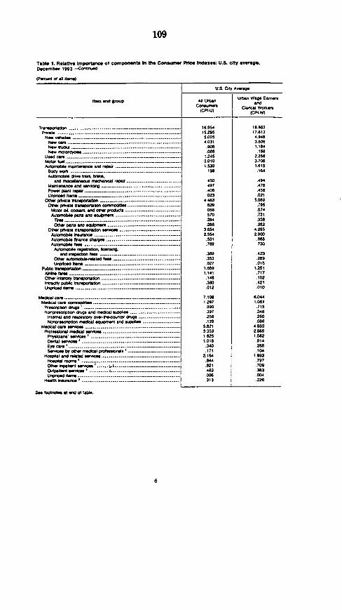
109
Tabil 1. Relatve importance of components In tiv. Consumer Price Indxese: U.S city averag.December 19J3 -Corwnd
(Peoer of 601.0.8e
U.S. Oby A-age
lum an, tr4up AD Uo UI.n Wage Eas
(CPI-U) ( WoIS6,
Trufpo abon ...... ...... __ ..... . __ .......... ...... ... ... ...... ........... 1e.954 18.B63r . . . ... _._............................. 15.295 17.813
NwOas .. ........... . _ . _._ 5.025 4.94BN . can, .. ..__....._._ . _.._ ............. ....._ _.__ ............ . 4031 3 SON WUn ...... _.___ .. ............ _.......... . .90B 1.184N Wro . . .. .. 0.. ................................ _ . .1
Ur.d e v r .... ...... 1.245 2.25Bmoor W . l ..... _ ._ ._._ ._ ._ _._.....__.. . 3.010 3.705A.ftobn e .r. ....... .... .... ._. 1.533 1.615
Body . ...... _ _. .................................. .S10 .184A6tonoo81 riv. nn b,
6Vd nrl l& r6eo 1 ............................ .. ... ... .450 .494r 6V d ne g 4978................... ._ ........... .497 .470
Po r repir ... 40...4............ __._... . .40 .458UO~o oreanl ... .2 _. *023 .021
Ote prialsloS tm ,. . . .... . ..... 4A4 .7a 5Motor or. W o r p ....................... .......... ._ .... O 5S .074Auo wbinle parts 64d aQqg nev .............................. 570 .721
Ti .. . ...... .. ... . . 284 338Otr pa va eqw .. ........................ . _ . _ _ ... .288 .3B2
008h P11. ouraptsuron . . .. 3854 4.295Ao56,0bil insurance........................ .... . . 2.554 28900A . r- rga ..................................................... 531 r885Aolo has . ................____.......... ... . . 789 .730
Automobie r.0 tim Iamd ho less .. . . ............................ .39 423
r0- 6b. d . ..................... . _ ..73 5 289
NW anpor n . .......... ... .._ 1.659 1.251Airlne a . ......... ... .. _ . ........................... 1141 .71709,6,Oy56ral, vale om ..................................... . . .148 .102lnuiloy pA t Owwpon . . 380 .421U, p adenw .... .................. _. .._ _ _ ._. .012 .010
Mod" cre-.- .............. ... ... ._._._ .- 7.108 6.044Medical cas .b...... . . . _ 127 1.061
P ea on r ............ . ............................................... B90 .715NorW-norton &.. nfed0wr ar,......... .. 397 346Intrral a nd rato ry rraa,-t 9 t WAP6 ............................ .......... .256 .260
rm socIa qprand Ripple .................... . . 13_ .096P001081 car ' . ...............-.... .. . 0.21 4.93ProD 'd ............ _ . . . . 3.353 2.865Pya c r .*. e... . 1._25 1.532D.l menaea . . ................... . ..................................... 1.019 .914Ey -r . _ .... . .. . ........... _ _. .340 .285
0r,6,cie r byow .ft.8 I0 ............ ... .11 .709Hospalad _ee .............. 3 ......................... 143 .3B3Unpnvd ... .............. . ................................. . 006 .004
H '0 . ............. ... _ . ................................ .313 22B
Sea f04t89866at 0o table.
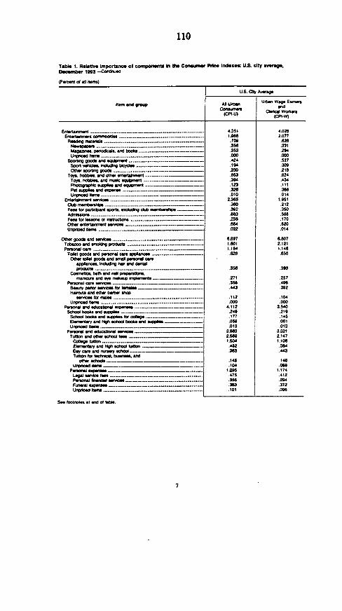
110
Table 1. Relative Importface of cohpofles In th e Cosne loe Indexes U.& dty average,Demb, bOBI -Cond
(PWcOM Of an de,,)
lts wwd -st$
Enl60Mtn _ __ _ ___.___ ___Eon ..a. 11-66.5. ._._._. ...... _... __ .......... _Ro1,. 110r 6 .olodha .h ......... .......... .
,fcw maeil ........................ .__. ........ _ -..--=-.
te aa~.' S005fl55_____
UdOe" .t.. ..___._._.._...__.__..___.___.
Spar _nlns. nodis- t. _ok._._.----.--
Topnco 11 xnd ottc .
Upticd vU=t _..__,
fe ak - ._ _s .._ ...... .. __._.__._.............. .... . ....... _ _ -- ----
Fesfo ptbVM t- a.ksV Cal---W~
Fees, for tssn vs mtrucuor0 ............ ....._......0ll t : __ . ................ _.___._ .............___.I
0_ 905d1s .. ........g.o..._ .. ..........Idw_Tobacco nd t . I .. .........................._.__ ...... ._ _ _PwsomrsM we
Toabt goodSod p 005 ---------t0w 1el pods sWd NMI -oe c'--appims bS~ hair d dera
oal .s .... ._ . ......... s. ___,_,_,
Beerty* parod O565 g~km lerre..wd
Hairs srld 0W- belts, M110Pl fo .__............. ............. __.......___........ ._.__...... -_ ------- -510006 Cd10 _ 11 __.__.___ . ..
Uvtol mbdeou...........___ _._U I 1 ._ . ...... ........ .... __._._.__......._
Prst and e ftal _ _...._ .0001book.so WO agplif
S00 books t4ad .___665 0__Elssol tw ard hg scrod books ad mapopEtny t14hsld tO114 1 __ _.___
eullonsi ram OlkdoJ .1__.._TIMM0 Ord Color_ _ _.__ =e
E tlA and high Khool Utlion _.Day canr and N" sdvoo _._ _ _ _Tdo for tooi tudas am
oVW, .d_.s. __. s__Urpiced . . _ _. -
L.9 s i fts .......................... __..... _._ ..__ ..... _.__.
Lsgsi IslaM tss
Ul o tema ........s.. _ ._.._ .o..t ._ ._._._._
Ses fwvwol *1 end Of tamI.
U.S. Mt AWae
A.lesa work|_~~~, Ut,- ~~~(ctW 'I-V
4.3511666.70S356303.000.424.194.2306B53
.394
.12t
.326
.0102.365
:20
.603
1.104
.35B
2.1
.443
.112-050
4.112.240.177050
013
3. SBB3
2.3561.504
452
.140
.104
.476
.2B8
.363
.13
.112
4.0202077
620331204.000527.309.21B.924.434.111366.014
1. 951.212350.5B.170.B20.014
6.6072.1211.14t.650
.393
.257
.406
.392
.104
.0003.540
.219
.115061013
3.3212.1471.106
.364
.443
.14B
1.174412264372.orc
A ........... ....... ___ ._..___.._
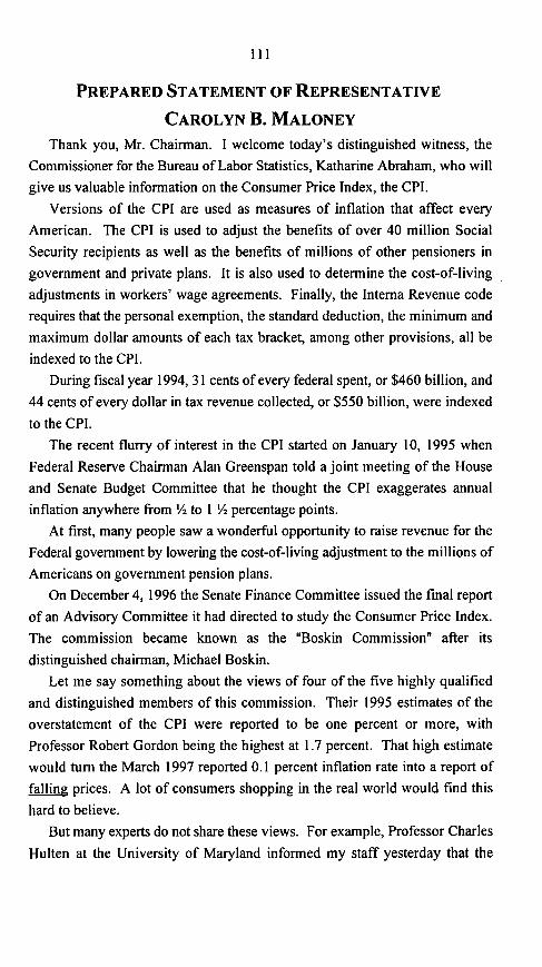
III
PREPARED STATEMENT OF REPRESENTATIVE
CAROLYN B. MALONEY
Thank you, Mr. Chairman. I welcome today's distinguished witness, the
Commissioner for the Bureau of Labor Statistics, Katharine Abraham, who will
give us valuable information on the Consumer Price Index, the CPI.
Versions of the CPI are used as measures of inflation that affect every
American. The CPI is used to adjust the benefits of over 40 million Social
Security recipients as well as the benefits of millions of other pensioners in
government and private plans. It is also used to determine the cost-of-living
adjustments in workers' wage agreements. Finally, the Interna Revenue code
requires that the personal exemption, the standard deduction, the minimum and
maximum dollar amounts of each tax bracket, among other provisions, all be
indexed to the CPI.
During fiscal year 1994, 31 cents of every federal spent, or $460 billion, and
44 cents of every dollar in tax revenue collected, or $550 billion, were indexed
to the CPI.
The recent flurry of interest in the CPI started on January 10, 1995 when
Federal Reserve Chairman Alan Greenspan told a joint meeting of the House
and Senate Budget Committee that he thought the CPI exaggerates annual
inflation anywhere from 1/2 to I 1/2 percentage points.
At first, many people saw a wonderful opportunity to raise revenue for the
Federal government by lowering the cost-of-living adjustment to the millions of
Americans on government pension plans.
On December 4, 1996 the Senate Finance Committee issued the final report
of an Advisory Committee it had directed to study the Consumer Price Index.
The commission became known as the "Boskin Commission" after its
distinguished chairman, Michael Boskin.
Let me say something about the views of four of the five highly qualified
and distinguished members of this commission. Their 1995 estimates of the
overstatement of the CPI were reported to be one percent or more, with
Professor Robert Gordon being the highest at 1.7 percent. That high estimate
would turn the March 1997 reported 0.1 percent inflation rate into a report of
falling prices. A lot of consumers shopping in the real world would find this
hard to believe.
But many experts do not share these views. For example, Professor Charles
Hulten at the University of Maryland informed my staff yesterday that the

112
errors in the CPI have not been estimated with enough accuracy to justify an
arbitrary adjustment in the CPI. Professor Hulten says that there are a number
of elements in the CPI that might understate inflation as well as elements that
might overstate inflation. He suggested that we should leave this adjustment to
the Bureau of Labor Statistics.
Joel Popkin, whose company has been estimating price indexes for many
years, wrote in his report for the American Association of Retired Persons that
the Boskin Commission's "conclusions are not convincing and provide no basis
for Congress to change federal indexation formulas that are based on the CPI..."
It is too bad that the Boskin Commission did not contain some of the experts
who do not believe its final conclusion of a 1.1 percent overstatement of the
CPI. The calculation of the CPI directly affects too many Americans to
arbitrarily change it on the basis of a controversial conclusion.
Noble Laureate Milton Friedman stated recently that "to manipulate [the
CPI] now is not good. In effect, an arbitrary adjustment of the CPI would
involve an increase in taxes."
I am asking my colleagues on both sides of the isle to support the resolution
I have submitted with my Republican colleagues Jon Fox and Phil English, and
my Democratic colleague Joe Kennedy. House Resolution 93 expresses the
sense of the House that the Bureau of Labor Statistics alone should make any
adjustments, if any are needed, to the methodology used to determine the
Consumer Price Index. We argue that the Consumer Price Index is only useful
if it is a technical , not a political measurement.
Our resolution has the support of the American Association of Retired
Persons, the Council on Aging, and the National Council of Senior Citizens.
I understand that the Bureau of Labor Statistics is in the middle of a six-year
program from 1995 to 2000 to make improvements in the calculation of the
CPI. I want to hear today from Commissioner Abraham about the progress
being made in that program and the budget needs for assuring the best possible
product.Thank you, Mr. Chairman.

113
CAROLYN B. MALONEY
*0i25.F4 2L;12) C-US
BANKING AND FINANOAL ° on-l' buts
GOVERNMENTRUFOBN- Congree; of the 1niteb Stated5OERSIGHT jtouse of Beprtntatibes
Ja.NT ECONOMIC C0-rr2EE)
Witbingtonl. MD 20515-3214
May 20, 1997
The Honorable Katharine G. Abraham, CommissionerBureau of Labor StatisticsUnited States Department of Labor2 Massachusetts Avenue, N.E., Room 4040Washington, DC 20212
Dear Commissioner Abraham:
It was a pleasure to receive your testimony before the Joint Economic Committee onMay 2, covering the Consumer Price Index (the C.P.I.) and the April employment situation. Iwas especially pleased to hear that the unemployment rate in April was 4.9 percent, the lowestit has been in almost 25 years. I do appreciate the fact that the statistics you presented arenational averages -- and as such do not reflect the condition of all workers. That said, I wouldcertainly appreciate your answers to the following questions:
I. The gap between wages for men and women appears to have narrowed over the lastseveral years, although there seems to be some discrepancies in the data. The gap inmedian annual earnings for year-round workers between men and women is reported tobe larger than the gap in median weekly earnings for men and women over the sameperiod. How do you explain this discrepancy? How are self-employed women treatedin the weekly and annual series?
Further, over the last several years, what has been the trend in the earning differentialsbetween men and women? And how does the Bureau calculate these earningdifferentials?
2. As part of the trend toward increased globalization, the value of U.S. imports hasalmost doubled over the last 10 years. Part of this increase has also been due to thecontinued strength of the dollar vis-a-vis the other major trading currencies. Has theBureau performed any research on what impact this significant increase in trade and thecontinued strength of the dollar has had on the C.P. I.? Are there estimates of whatwould have happened to the C.P.I. in the absence of these developments?
Given how important international trade is to the US economy and how much itdominates policy discussions, I would encourage you to make this issue a high priorityfor your Bureau's research agenda. I would appreciate if you would share with me, aswell as with the other members of the Committee, any findings as soon as they becomeavailable.
Juno of word *

114
Page 2
3. 1 understand the Bureau recently announced some changes in the way it calculates theConsumer Price Index. Would you please describe the types of improvements you havealready made, as well as those the Bureau plans to make over the next several years'?Can you provide an estimate of how much lower or higher the current C.P.I. wouldhave been, had these changes already been in place over the last year'?
4. According to the Bureau's statistics, the unemployment rate for New York City isapproaching close to twice the national average. Can you provide any further details --including break-downs by age, sex, race, education and occupation -- which might helpexplain this large differential?
I look forward to receiving your answers to these questions and to furthering our dialogue onthe condition of American workers.
Sincerely,
Carolyn B. MaloneyMember, Joint Economic Comfnittee
cc: The Honorable Jim Saxton, Chairman, Joint Economic CommitteeOils. Colleen Healy

115
U. Deparinat of Labor CmreasonerBureau of Labor Statis~csWasNngtonD.C. 20212
.AL 1 17
Honorable Carolyn B. MaloneyHouse of RepresentativesWashington, D.C. 20515-3214
Dear Congresswoman Maloney:
I am writing in response to your letter of May 20, in whichyou requested information on the female-to-male earningsratio, the effects of international trade on the ConsumerPrice Index (CPI), planned improvements to the CPI, and theunemployment situation in New York City.
Your first question concerned differences in measured annualand weekly earnings for men and women. Earnings data fromthe Current Population Survey (CPS), a monthly survey ofabout 50,000 households that is the primary source ofinformation on the Nation's labor force, are widely used toexamine trends in the women's-to-men's earnings ratio. Twodifferent measures of earnings typically are used for thispurpose: (1) median annual earnings derived from the Marchsupplement to the CPS, published by the Census Bureau and(2) median weekly earnings derived from a portion of themonthly CPS sample, published quarterly by the Bureau ofLabor Statistics (BLS). In 1995, the women's-to-men'searnings ratio based on the annual earnings figures was71.4 percent for persons employed year-round, full-time.The ratio based on the monthly CPS data was 75.5 percent forfull-time workers.
Both these ratios are simple comparisons of the earnings ofall the men and women in the defined universe. There are nocontrols for differences between men and women in measurabledemographic or work-related characteristics, such as age,education, and experience, nor do the ratios take into-account differences in men's and women's occupationaldistributions.
There are several conceptual and methodological differencesbetween the annual and weekly earnings data series. Forexample, the annual earnings estimates include earnings fromall jobs held during the year and earnings from both wageand salary employment and self employment. The weeklyearnings estimates pertain to the primary job only and

116
Honorable Carolyn B. Maloney--2
JL I 7 W97
include only wage and salary earnings. Given thesedifferences, it is not surprising that the women's-to-men'searnings ratios based on the two data series differsomewhat, but we know of no research that allows us toidentify the specific contributing factors.
Regarding the trend in the women's-to-men's earnings ratio,I have enclosed tables that show the BLS data series onmedian usual weekly earnings for women and men from 1979 to1996 by various characteristics, as well as the women's-to-men's earnings ratio for that period (see Enclosures 1, 2,and 3). As you can see, with the exception of a brief pausein the late-1980's, the women's-to-men's earnings ratio rosesteadily from 1979 to 1993. Several factors contributed tothe shrinking of the female-versus-male earningsdifferential over this period, including rapid increases inthe educational attainment of employed women and themovement of women into more highly paid managerial andprofessional occupations. Between 1994 and 1996, theoverall ratio of women's-to-men's median earnings edgeddown, although, as shown in the enclosed tables, there hasbeen some variation by age, education, and level ofearnings. (The decline in the women's-to-men's earningsratio in 1994 reflects, at least in part, the major redesignof the CPS that took effect in that year.)
The recent decline in women's relative earnings may reflecta number of factors such as the impact of the business cycleon earnings, secular changes in occupation and industryconcentrations, and the trends in women's and men's years ofwork experience and level of educational attainment.Sorting through these various effects would require in-depthanalysis that is beyond the scope of this letter.
In response to your second question, BLS has not conductedstudies of the impact of international trade and imports onthe overall CPI since the major revision of the index thatwas implemented in 1987. Prior to that revision, the CPIprogram had a general provision for "Country-of-origin"

117
Honorable Carolyn B. Maloney--3
JAL 1 7 MT?
codes, which enabled us, with limited success, to identifyimported items and track 'their direct contributions tochanges in the CPI. over time, however, we lost confidencein the accuracy of our measurement of the importance ofimports. It is relatively easy to identify imports at theborder, as goods are shipped into the country, but much moredifficult in retail outlets. The difficulties may be asmundane as labels indicating country of origin beingconcealed by plastic packaging. For items in manycategories-produce is a good example--country-of-origininformation may be burdensome for our respondents to supplyand thus difficult for us to collect. Difficulties alsoarise as a consequence of the production and distributionsystem having grown more complex. Many goods are producedby multinational firms, and the determination of such items'foreign content is subject to the sometimes-arbitrary cost-accounting procedures of those firms. A furtherconsideration is that imports may have indirect effects oninflation that our direct measurements of imported goods'prices could not capture. Increases in the price ofimported oil, for example, will affect the prices oftransportation services, which contribute to the retailcosts of many items. Conversely, import competition mayconstrain the ability of domestic firms to increase prices.
I should mention that for some items, particularly in theapparel area, we have resumed the collection of dataregarding the country of origin over the past four years.For these items, country of origin has become more importantin advertising and may affect the perceived quality of theitems.
As a general matter, the BLS has focused its researchefforts on the improvement of its measures. Whileinteresting and important, the relationships betweenexchange rates and import prices, and between the volume ofimports and the pricing behavior of domestic firms, aresubjects in which the BLS has no special competence.
In response to your third question, which concerned past andplanned future improvements to the CPI, I am enclosing an

118
Honorable Carolyn B. Maloney--4
JU. 1 7 1997
additional copy of a paper, entitled "Measurement Issues inthe Consumer Price Index," that we recently furnished to allmembers of the Joint Economic Committee (see Enclosure 4).This paper was requested by Congressman Jim Saxton in aletter dated January 28, 1997. As noted on page 9 of thispaper, in 1995 and 1996 we made several changes to eliminateformula bias in the CPI; we have estimated that thesechanges reduced the rate of growth of the index byapproximately 0.24 percentage point per year. In addition,we are currently investigating an experimental CPI that usesa geometric mean formula in the calculation of CPI componentindexes. As noted on page 25 of the paper, partial adoptionof this approach in the official CPI would be expected tohave a downward impact on its growth rate of between zeroand one-quarter of one percent a year. Other changes thatwe have made and that we have planned include the January1997 change in the hospital and related services componentand the January 1998 updating of the CPI market basket.These and other improvements are discussed in the concludingsection VII of the paper.
In response to your fourth question, I am enclosing a seriesof tables that may shed light on the joblessness situationin New York City, per your request. Unemployment in NewYork City has been above the U.S. average over most of thepast 30 years, with 1987 and 1988 being the most notableexceptions (see Table A). The jobless rate in the citybegan to rise before the most recent national upturn and,unlike the rate in most areas, has failed to return to pre-recession levels (see Chart 1). In 1996, New York City'sunemployment rate was about the same as that for some othermajor cities, such as Los Angeles and Washington, D.C.,places where the 1996 rate also remained well above the 1990figure (see Table B).
For all major demographic groups in the city, labor forceparticipation rates and employment-population ratios aresubstantially lower than the U.S average, and unemploymentrates are noticeably higher (see Table C). New York'sunemployment rates are also well above the U.S. average formost major industries and occupations (see Tables D and E).

119
Honorable Carolyn B. Maloney--5
JL I 7T9O
A substantially-larger-than-average share of the city's
employed population is comprised of African Americans andHispanics (see Table F).
I hope you find these responses to be informative and the
enclosed materials useful. If I can provide further
assistance to you on any of these topics, please let me
know. Philip Rones, Assistant Commissioner for CurrentEmployment Analysis, on 202--606-6378, would be happy to
answer any followup questions from your staff concerninglabor force data and John Greenlees, Assistant Commissionerfor the Division of Consumer Prices and Price Indexes,
on 202--606-6950, may be contacted regarding the CPI.
Sincerely yours,
KATHARINE G. ABRAHAMCommissioner
Enclosures

120
YNS MALONEY ' _ eE- IC- ~ ~ ~ ~ ~ ~ ~ ~ ~ ~ ~ ~ ~ ~ ~ ~ ~ ~ ~ - 'O~~ N
3s.. : .I-c. . ? a fl 4 t. 0.....-''°. s
. A CA 0. 26.st ,: *4. H
SERvICEs _
!srWv Er- COngre~s of tie Zniteb states5`,E AS~ Irr 1ouge of r;eprefmntutibeg - ... -..S,NOM'C COM.MEE 5- of
Warbington. OC 20515-3214
May 20, 1997
The Honorable Katharine G. Abraham. CommissionerBureau of Labor StatisticsUnited States Department of Labor2 Massachusetts Avenue, N.E., Room 4040Washington, DC 20212
Dear Commissioner Abraham:
It was a pleasure to receive your testimony before the Joint Economic Committee onMay 2, covering the Consumer Price Index (the C.P.I.) and the April employment sinuation. Iwas especially pleased to hear that the unemployment rate in April was 4.9 percent, the lowestit has been in almost 25 years. I do appreciate the fact that the statistics you presented arenational averages -- and as such do not reflect the condition of all workers. That said, I wouldcertainly appreciate your answers to the following questions:
I The gap between wages for men and women appears to have narrowed over the lastseveral years, although there seems to be some discrepancies in the data. The gap inmedian annual earnings for year-round workers between men and women is reported tobe larger than the gap in median weekly earnings for men and women over the sameperiod. How do you explain this discrepancy? How are self-employed women treatedin the weekly and annual series?
Further, over the last several years, what has been the trend in the earning differentialsbetween men and women? And ho" -acs the Bureau calculate these earning
'differentials?
2. As part of the trend toward increased globalization, the value of U.S. imports hasalmost doubled over the last 10 years. Part of this increase has also been due to thecontinued strength of the dollar vis-a-vis the other major trading currencies. Has theBurcau performed any research on what impact this significant increase in trade and thecontinued strength of the dollar has had on the C.P.I.? Are there estimates of whatwould have happened to the C.P.I. in the absence of these developments?
Given how important international trade is to the US economy and how much itdominates policy discussions, I would encourage you to make this issue a high priorityfor your Bureau's research agenda. I would appreciate if you would share with me, aswell as with the other members of the Committee, any findings as soon as they becomeavailable.
CAROL.a... ),
3OVET. C
,O.NT ECO
.1
I-22
.......
'i"II.
W

121
Page 2
3. 1 understand the Bureau recently announced some changes in the way it calculates theConsumer Price Index. Would you please describe the types cf improvements you havealready made, as well as those the Bureau plans to make over the next several years'Can you provide an estimate of how much lower or higher the current C.P.I. wouldhave been. had these changes already been in place over the last year?
4. According to the Bureau's statistics, the unemployment rate for New York City isapproaching close to twice the national average. Can you provide any further details --including break-downs by age, sex, race, education and occupation -- which might helpexplain this large differential?
I look forward to receiving your answers to these questions and to furthering our dialogue onthe condition of American workers.
Sincerely,
Carolyn B MaloneyMember, Joint Economic Co! i.ttee
* cc: Xhe Honorable Jim Saxton, Chairman. Joint Economic Committeevfvs. Colleen Healy

so -I
.1h .....
a6 Y.- -3 $2.0 $26. $263 $102 $313 $326 $343 $]SO $37) S) II 'IO I 'IO .. 2, $3, %.-I $426 TO 54 9 $':67 S. 9 62-:0
2 ........... III 187 3 331 2.2 2:I 29 1 "I "I 25*2 2 292 4. I:: .3 I.. . 11. I., 195 20' ass I.3 .1 I.
20 1. 2 11 4S'S 21050' 2.) 22 I'll II.,! 1110.I Y 2: 112 110 110 "I IS, 11, 1125 . ......... I&, as& .I . 41 .27 4.1 4 .1. ... I" 'IO
28, 3a� I:S. I.......... 316 IO 1 31. 3.2 319 391 .03 "I 5 11, .1as a 'S ), lo) 31 : 1.01 : I's :1112 : 1124 I 0.19 .11': � I....... 21S .,S III I'l I' 121 1 1 11 IIl IY . a a I ... ... I. 7 51, Ss.
.5 lo S.' :::::: 2"'o. 2'al' MO Us M I':91 :0'0' : 11' 121 412 .72 ..: 11:11 5"21 IS412 S.. 542 11 "I55 Y.... . ..... ass 276 3W 319 33, 356 314 38, 39. I11 I
SS - 64- ... 36 1 : 31 ! :110, 4 1 I :21 slo? 11 I 1.':4 IO' M' a ' I I '*O " 60' I I I I. "IIs Y- -d ... all I 3 211 25 1 0 271 .1. 219 1�0 III 11, I,) )9a l a,, as, Is,
"'.I. 16 `-', -` a 3is - 24 - N" 20'.' I' ? ; I'2': 2"Ill 2' 91 II 2. I41"I N " 2' : Z IN! N1 NI 3.1 4� 3' I� .6 I29.2 I'. I'71
`- ... .... .
10,
16 - I Is. .. a.20 3: ilo I, 11 all .111.0 �1111 .1110, I'll, .1:11 .11, 5 21" III, I 11 : 11 1: 11 11 11 I I I 13,
25 31. 33, 31311 M ..6 .22 1 4 2. .62 .7.1 4 0'7' 5000 S12 52) S36 5505 570'. 53 $I So S3 12 9�as 5. 'IO "I M 101 411 - "I 11 1: ll'� III '31 III s7l I.. 'I:
�' 9, a. I, .. .. .I '.3 :5 a, :I. :'I, '4 Y- I" I III I 9
5.2 siois I. -1:.... I, a,:,. " '9 " .4 "109 " a " 1-1 ll� N.' I I
13 109 : 32 ; Is, .1 10, "I "I S- I. 376 $91 6.I 62:SS '. 6 1 3'. as 461 ..: ::ll Soo I, 1. S., 5': ... .01 'a 3.1 I' "2: 2"66 300 Os 327 367 358 IGO 394 393 1 06) 467 421 4SI ..I .41 477
`-.1 It -d - 10, III 21, III 11 117 11 101 I I'l 11 14 1:: M II) M 4.6 -11 i. 24 ......... 154 I', I.0 ,I III I.) II0 2�: .. . I.: ": a '67 7 '.
11 21.1 V r....... 13i 1.5 .5. S7 158 III IGS III 171 III 117 ass 21.. IO' 'OS .. 31520 Y ........ III 17. .. I 211 210 2.0
as � . I S! 2'al' �' .1 'I I' 12 'I 1. I I. I 331 slot III 1.1 2 1.11 1.92 01 11 21 .1 .1:1.$1 2�. :" 4' .I 42S .13
25 o 3 N 215 256 211 285 216 110 323 31. V-1 ....... .99 218 219 257 211 ": '.'O' 33 'S 'I 3sol 3 002 315 391 .03
25 1 I 'I 'I 1.1 : I .1" 211 1 .1" ':' `5 IO' "I 32 3 411,6: - 2 I 1.1 O. '. '.'4. 'S' 'IO 191 10: 19 101 411.S I I a I as. I ... .,I as ,7 3,, as :,7 :. :16 ::Iso
SS -6 211 ':.' "I' 22' ':.' 1 M 320 3.2 ass 371 30, II 10,::::: la I':2. 2a. I 1 7 1 I Its 3:0 1.1) :z
.1 I 21. I, M 3)6 353 11.
II=. 1:1 I Io :s o 1. A.Bs._. of -_ ..e -_ acl-.. -t he r1e ae

7.60 . 2 343. aa..e _a.6y earnnol o. .81 6.313. . .oal I . by a... .e.. a... _. e~fleye tyr~iet. OrtlsYtyC., 5 -IIY ...0lvy 3.1elld 81n4lover.... l7s.56
total. 16 roar. .6d oyer. .............. 62.5 66.6 66.6 65.4 66.7 67.8 66.2 682. 70.0 70.2 70.1 70.9 76.2 75.6 77.1 76.4 75.5 75.016 C0 26 Yaara. ............ 76.6 80.3 82.6 65.3 68.2 67.9 67.5 69.0 67.9 93.0 90.6 90.2 93.3 p6.0 94.6 93.0 30.8 92.5
66 t- 10 V-- ......... 05.1 69.5 92.3 92.6 94.6 92.5 90.7 6.4 67.7 69.6 94.3 90.6 3.6 96.3 92.8 2.3 66.I 66.620 C0 26 Va . 76.7 76.0 0.6 82.4 65.9 85.2 6..7 67.5 60.0 90.0 69.7 60.3 93.7 94.3 5. 93.5 92.4 92.
25 year. ad over.. 6 62.5 6 2.8 64.6 65.6 664. 67.0 66.7 67.3 66.9 7 0.2 72.I 74 0 74.6 768 73.3 72.9 76.25 CO 54 Vers ...................... 62.3 62.9 61.2 65.1 667.3 67.7 67.6 .5 60.0 69.7 7.1 73.0 74.9 7 5.6 75.6 73.9 73.9 75.
25 O . ....... 67.5 61.. 705 70.0 77.2 7.3 751 7 7 .6 7.7 7 .0 62.0 63.0 92. 8.2 6.3510O 4 e ........... .56f.2 58.3 59.7 43.3 63.3 63.6 63.2 64.1 65.9 60.3 66.3 69.6 70.6 71.9 73.0 70.7 72.6 77.065 Ca S. . 5 6 5... 6.0 .3 59.0 59.6 6..0 62.6 61.7 60.7 63.8 65.0 65.8 67.6 67.1 7.7 69.9
55 .aar 69 o'er 63. . . .... 62.3 63.6 61.1 62.2 62.7 6.1 60.9 65.0 65.0 67.5 66.2 5.3 I 5.355 .. 66 569-3. 63.8 61.0 60.. 6..0 62.2 62.4 63.7 64.5 66.9 67.6 660 6.7 65.)65 rear, nd over 0 .7.6 76.3 70.7 70.3 69.5 66.7 65. 71.2 68.6 70.8 76.3 76.4 66.3 77.9 76.3 70.3 60.0 70.0
total. 36 year. oaa ever 63.7 63.3 43.0 66.3 65.6 67.0 67.4 67.9 66.2 69.4 69.3 73.5 72.7 75.1 76.5 76.6 73.3 73.606 C to e r 2.............77.9 79.2 82.3 66.0 67.7 66.8 66.5 66.0 67.1 69.0 69.9 69.5 92.7 93.0 92.9 93.6 90.6 92.325 year. n , l ovar.61.4 60.6 3.6 66.2 65.3 66.I 65.6 6 5. 6 66.6 .4 6 . 7 710.9 73.2 72.7 7. 73. 72. 72.7 76.1
25 10 50 ya . 61.5. ........... .6ls2.2 02.5 66.7 05.9 67.0 66.0 66.3 67.9 69. 5 70. 72.9 73.6 73.9 76.0 76.0 73.6 75.455 .ear. a nd any. 60.7 59.6 76.5 63.0 63.3 61.6 60.3 60.6 63.6 63.9 63.7 62. 6 64 66.6 65.3 66.9 66.0
total. 16 rear. .00 alloy.. 76.6 75.9 76.5 7.0 79.8 79.l 92.9 62.7 66.6 63.0 66.5 65.3 06.1 99.2 69.9 66.5 96.4 97.936 to 26 r 0 . 66.. ,,t2 91 .3 69 .0 32.7 94.8 90.9 97.0 90. 96.7 97.3 96.3 96.0 87.6 94.5 101.6 87. 9 8 4.925 Veara aS over ...... 73.2 7 3.5 75. 0 76. 6 76. 0 77.7 61.5 60.5 60.6 79.6 62.8 862.7 85.6 17.3 07.9 96.9 63.9 96.
25 to 56 yara . 73.9 73.9 75.6 76.9 76.0 77.9 62.2 60.3 60.7 60.0 60.3 63.0 85.7 60.3 6.3 66.3 2.a 6.655 Ver .0 od Or . 73.6 ... 73.8 73.6 72.3 72.2 70.6 76.6 75.6 63.6 73.5 76.0 79.7 91.6 76.9 92.9 76.9 79.0 79.0
total. 36 aerar aod11alver._. 60.6 82.0 66.7 65.6 67.0 90.4 99.1 90.5 66.9 67.3 89.816 CO 26 Vya6 . 95s.8 95.9 96.9 95.3 93.6 92.9 306.6 96.8 92.9 90.2 000.025 Y.- o r7 6 637 61.4 90.6 63.6 64.3 66. 6._0 63.2 64.9
25 tO 56 Y.: ........ 73.0 79.6 66.9 63.6 92.0 66.7 95.6 67.7 95.7 9.7 95.655 net. ar Ollol...................... _ _ ........ _ _ _ _ _ 71.1 76.6 76.5 77.5 07. 7 76.9 66.6 72.9 70.6 76.6 63.7
aaya ze63.e tab1al6O_ len 16 Carreet ea.3t1aee.. 2.6. 90r3 06 -400 bae eC Ler 611666a ea C 681 .0larlr* Oeo. t.I -Iee V*trOClly Cay63 l31 ale XCa .aylter year..
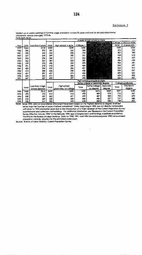
124
Enclosure 2
Median usual weekly earnings of lu-time wage and salary workers 25 years and over by sex and eductiotnaloattrnment. onnual avertoe$ 1979-96t-otI brht sem rs
Year Total Less than 4 years
1979 5265 S2101980 286 222
1981 308 2401982 327 2481983 343 2561984 362 2631985 379 2701986 391 2781987 403 2841988 414 288
1989 427 2971990 449 3031991 467 307
1992199319941995IWo
total Less than a highI school dpbmloen
$480493soo510520
S312316307309t17
4vrColee. 4 Years or more
Total Iif h school. 4 years Cotee. 1 Total 4 years onty$280 S249 S282 _344 S320302 266 304 376 352324 286 324 407 385349 302 351 438 410365 311 363 461 423382 323 382 486 454398 333 399 506 481410 344 409 525 497422 356 421 564 513438 368 430i 585 527457 375 452 609 563477 386 476 638 595490 397 489 666 607
_Hifno school graduate or moreSeec aeeo ssociate deareeI Clai rdee
Total Ho schoe Tt Some ca Assocte Total Bachebrmsroduetes no cotleg o no degree degree deoree
S499 $404 S485 S475 $509 $697512 416 495 484 519 716522 421 499 487 522 733538 432 508 496 537 747Ski6 443 518 504 556 758
$640661670686697
NOTE Siice 199Z data on educatIonal attainment hove been bared on the hloghest dploma oa degree recehled'rather than the "number ot years ot school completed.' Data. beginrging 199I 4 aTe not drectly comparablewith data for 1993 and eaeler years due to the introducton of 0 major redesign et the Current Population Surveyquesfannaire and colectn methodology. For additional intormdnorl. see T'evisons hi the Current Popuk7tionSurvey Effective January 1994,' in the February 1994 issue at Employment and Eamings a periodical pubtshedmonthly by the Bureau ot Labor Stadstics. Data tor 1990, 1991. and 1994 tonwerd incorporate I190 census-basedpopulation controh odjusted ter the estimated undercount.
Source: Bureau o1 Labor Statistics Current Poprulattn Survey
_ � � ._
I
l V Wow z . . - - - - _ - -__, , _ -

125
Median usual weekly eofnlgs ot tat-le wage and salary workers 25 years and over by sex and educationdotranrenr annud averages. 1979-96Totaln men
1979198019811982198319841985198619871988198919901991
I -A.. LrS-Ohr
sJro339372393407422443463477487500512523
S5y267286293301308314321324332346349349
rt 8
19921993199419951996
total Less than a highschoo I -do--
559576588SW9
360342347357
4 Years of h- h school or mare
l-C o h s c h o o l Totad u a teeorssn o re
Total Igh scho ol 4 ye tol Some c g s o ea ch or e
S363 33207 359 Ii i ll i s4297 548i393 356 38 o | 475 453
415 374 4 503 489430 388 422 no d e I deare 518 500453 399 446 * 562 523476 407 472 55 * 50 7488 416 485 ** 618 587499 423 47 ** 653 608510 437 53 * 679 621523 450 .517 s i 705 650547 459 542 * 741 683567 470 563 |11II 6 0
SHlah schoo Orroue orMr
Hig scoo Some cdleae or essocite^ dermee I Collgea g aduetes
Tod raduaese5 no coflea T.of I |Samedb0 Cllee Associate I Told I .... e~ciree
S579 S480 8 557 | $541 I $587 I - 793592 488 574 564 591 807607 496 587 578 607 826618 507 596 588 613 845631 516 604 593 6285 7
5736767756771
NOIE Since 992. data on educatioral attarnment hove been based on the _6ghest dpkoma or degree tecereer-rather than the 'number o1 years oa school completed.' Data, begirrnig In 1994, are not directly comparablewth data tor 1993 and earser years due to the inroductlion oa a major redesign of the Cunent Populodlon Surveyquestionnakre and colection methodology For additonal infonnation. see SRevisiogu in the Cunent PopulatenSurvey Etfectrie January 1994.' in "e February 1994 issue at Employment and Earnings a peroolcol publishedmontihly by the Bureau at Labor Staflstics. Data for 1990, 1991, and 1994 forward incorporate 1990 census-basedpopulation controls adjusted for the estimated undercount.
Source Bureau oa Labor Statistics Cunent Populaion Survey.
41-721 97 - 5
-1
=._ | 1 ---- -- '- ---- h=l | ' '- -- B'-- | --- | | -- U'-I M_1 h^/l tIIF/IUI I Wu
ARtO [ < tM
..- - --. -.__._- --.. _.. ..... .... E_..._ _ . . , _ /YU)
-
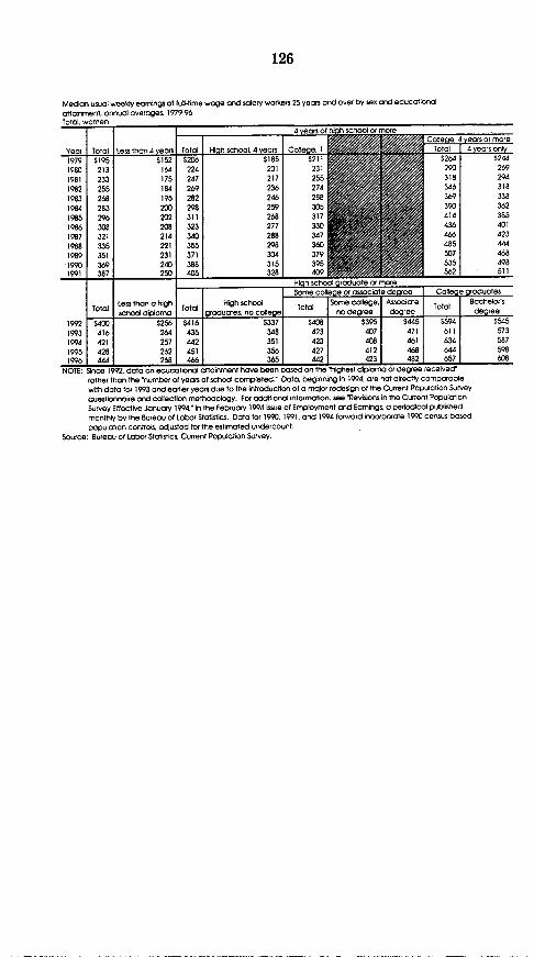
126
Median usuol weekly earnrngs of fu3-tlme wage and salary workers 25 years and over by sex and educational
attainment annual averages. 1979-96T-1J, v---e
Year Total Less than 4 years Total Hiph -sCh1Ol 41979 5152 S206
1980 213 164 2241981 233 175 2471982 255 184 2691983 268 195 2821984 283 200 2981985 296 202 3111986 308 208 3231987 321 214 3401988 335 221 3551989 351 231 3711990 369 240 3881991 387 250 405r
1992199319941995
Less than a highTotld school dlotran
5400416421428
$256264257262
TodaraduraTes nocrS416 _435442451
4 Yearsyaee.4ears or more
rears 4Cote. I Total 4 ears onl$185 8211 236 5244201 231 290 269317 255 318 294236 274 346 318246 288 369 338259 305 390 362268 317 414 385277 330 436 401288 347 466 4233298 360 485 444304 379 423 468315 395 531 498
Hiatt school graduate or mareSome coe ear associate de ree Callege graduates
Some college, Awsociate Ttl Bachelots.Ilege Ttl no degree degree degree$337 S408 $395 S445 S594 5545348 423 407 471 611 573351 423 408 461 634 587356 427 412 468 644 598365 _ 442 423 482 657 608
NOTE Since 1992. data an educational attaimnmrent hove been based on the 'highest diploma r adegree *eceived-rather than the 'number of years of school campleted. Data. beginnvsg In 1994. are not directly comparable
with data far 1993 and earlIer years due to the Introductian ol a major redesign of the Current Population Surveyquestionnaire and coalectlon methodology For additional intormation. see *Revisions in the Cunrent PopulatianSurvey Effective January 1994; in the February 1994 issue of Employment and Earnings. a periodical pubilshedmonthly by the Bureau af Labor Statistics. Data Tor 1990. 1991. and 1994 forward inootpadte 1990 census-basedpopulation controls. adjusted for the estimated undercount
Source: Bureau of Labor Statistics Current Population Survey.
_. .__ _., _. = 1, __
_ _ # ..,wo r zr I

127
Med an usual eeldy ear-ngs of lt-time wage and sagory workers 25 years and over by se. and educatronalattaonment. annual a-eroges. 1979-96Womens-to -- en's ernns-tin
-Y r ol 55r n e5 ol_ ihsho 4 v ears
YerITtlILess than 4 years IToald I th school. 4 yearsI Cotege.62.162862.c64965.8967.166.866.567368.870.272.174.0
74.473. I72.874 1
vO.~61v61.62.641.64.164.164.866C66.466.868871 6
Less than a highIo~ school delslm
7A '7^72.1
73.375.175.575 1
61 .7612762.864.865.6665866366.268.169.670.970.97.1
601
61.361 C63.163.464.5
66.8
68.168.2676.68.6AO A
HIgh scSomec
ga~ raduates, no cotege -o~
idut orme !ee. 4 years o more
oi e or associater dearee Co es roduateIsome college. IAssociate Ttl Bactrejars
no d degree degreeTotal
no degree I degree 6, de 64ee
71.8 70.2 73.2 73.0 75.8 749 _73.5 71.3 73.7 72.2 79.7 75772.8 70.8 72.1 70.6 75.9 76.873.0 70.2 71.6 ' 0.1 76.3 76.273.9 70.7 73.2 71 .3 77.1 752
NOTE: Since 1992. data on educational attairment hove been based on the 'highest diplomra or degree recehed'rather than the number o0 years of school completed. Data, beg nning In 1994. are not directly comparablewvith data tot 1993 and eadier years due to the introduction al a major redesgn oa the Current Population Surveyquestionnaire and collection methodology. Far additlonal inlormation see 'Revisons in the Current PopulationSurvey Effective January 1994, in the February 1994 issue of Employment and Earnings. a periodical publishedmonthly by the Bureau at Labor Statistics. Data for 1990. 991, and 1994 forword incorporate 1990 census-basedpopulation controls, adjusted tor the estimated undercount.
Source: 8ureau ot Labor Statstics. Current Population Survey
74.075.7776.77 6
Myyy
1980198119821983198419BS1986198719B3198919901991
1992199319941995l996
/O.2
__
- _ . -. I

Enclosure 3
Table 2. Usual weekly earnings of full-time wage and salary workers 25 yearsand over, by upper limits of selected quartiles and deciles, 1979-96 annual averages
Upper limit of Upper limit of:
First First Second Third I Ninth First First Second Third Ninth CPI-U
Year decile I quartile I quartile (median) quartile decile decile I quartile quartile (median) quartile decile (1982-84=100)
In current dollars In constant (1996) dollars
1979 $135 $185 $265 $369 $493 $292 $400 $573 $797 $1,065 72.6
1980 146 199 286 399 522 278 379 545 760 994 82.4
1981 159 215 308 430 582 274 371 532 742 1,005 90.9
1982 167 228 327 467 619 272 371 532 759 1,006 96.5
1983 175 238 343 487 658 276 375 540 767 1,037 99.6
1984 181 249 362 507 699 273 376 547 766 1,056 103.9
1985 185 258 379 522 730 270 376 553 761 1.064 107.6
1986 190 267 391 550 764 272 382 560 787 1,094 109.6
1987 195 277 403 577 798 269 383 557 797 1,102 113.6
1988 202 285 414 596 824 268 378 549 790 1,093 118.3
1989 209 293 427 617 867 264 371 540 781 1.097 124.0
1990 220 304 450 646 909 264 365 540 775 1,091 130.7
1991 230 314 468 674 950 265 362 539 776 1,094 136.2
1992 234 321 480 694 982 262 359 537 776 1,098 140.3
1993 241 331 493 716 1,000 262 359 535 777 1,086 144.5
1994 238 331 500 738 1,035 252 350 529 781 1,096 148.2
1995 244 339 510 754 1,069 251 349 525 776 1.101 152.4
1996 250 348 520 771_ _. r} . _ IA*:__ . . C 1,11 3, 250, 348 520 771 1,113 156.9
Source: Unpublished tabulations from the Current Population Survey, u.b. UepaILIrIilt VI LdJUI, ureaU VI -. aV .,-- y--
are not strictly comparable with data for earlier years.
T-1~z hnh - -F
I
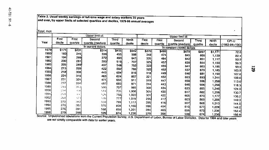
Table 2. Usual weekly earnings of full-time wage and salary workers 25 yearsand over, by upper limits of selected quartiles and deciles, 1979-96 annual averages
Total men
._T -First .. Upper limit of: Upper limit of:First First Second Third Ninth First | First Second Third Ninth CPI-UYear decile quartile quartile (median) quartile decile decile quartile quartile (median) quartile decile (1982-84=100)In current dollars In constant (1996) dollars
1979 $171 $231 $314 $415 $542 $370 $499 $679 $897 $1,171 72.61980 183 249 339 455 598 348 474 645 866 1.139 82.41981 194 269 372 493 647 335 464 642 851 1.117 90.91982 200 281 393 519 707 325 457 639 844 1,150 96.51983 205 289 407 548 752 323 455 641 863 1.185 99.61984 213 299 422 582 785 322 452 637 879 1,185 103.91985 218 308 443 604 816 318 449 646 881 1,190 107.61986 224 316 463 624 867 321 452 663 893 1,241 109.61987 231 324 477 656 911 319 447 659 906 1,258 113.61988 237 334 487 683 971 314 443 646 906 1,288 118.31989 ;!14 :W.1. 5(0 707 985 309 434 633 895 1,246 124.01990 : * 1 735 1,006 305 430 617 882 1,208 130.71991 .,, 758 1.022 301 422 605 873 1,177 136.21992 .jL,4 :. .i,3 777 1.078 295 417 603 869 1,206 140.31993 272 :Ii3 5s9 799 1,117 295 416 607 868 1,213 144.51994 270 382 576 828 1,160 286 404 610 877 1,228 148.21995 276 391 588 850 1,201 284 403 605 875 1,236 152.41996 279 398 599 874 1,236 279 398 599 874 1,236 156.9Source: Unnublished tabulations from thp rimprnt Pnn.,I~tlnn "--n, I I Q fl --- - .-' I - .- -†… ~ ~LUI nurea-u _ 01 .~ braists uai r 199 an ae erarce: not strictly omparable with data for eri yerren Po zulars.n SU vev Bur Of L U I 1994 and .: yearsare not strictly comparable with data for earlier years.

Table 2. Usual weekly earnings of full-time wage and salary workers 25 years
and over, by upper limits of selected quartiles and deciles, 1979-96 annual averages
Total, womenUpper limit of: Upper limit of:
First First Second Third Ninth First First Second Third Ninth CPI-U
Year decile I quartile uartile (median) | quarti le decie quartitle quartile (median) uarile decile (1982-84=100)
In current dollars In constant (1996) dollars
1979 $110 $146 $195 $260 $338 $238 $316 $421 $562 $730 72.6
1980 128 159 213 287 375 244 303 406 546 714 82.4
1981 138 175 233 315 413 238 302 402 544 713 90.9
1982 144 187 255 346 451 234 304 415 563 733 96.5
1983 150 196 268 367 480 236 309 422 578 756 99.6
1984 155 205 283 389 509 234 310 427 587 769 103.9
1985 159 212 296 410 532 232 309 432 598 776 107.6
1986 165 221 308 427 570 236 316 441 611 816 109.6
1987 172 231 321 455 601 238 319 443 628 830 113.6
1988 178 240 335 476 630 236 318 444 631 836 118.3
1989 185 250 351 497 675 234 316 444 629 854 124.0
1990 194 263 370 519 711 233 316 444 623 854 130.7
1991 205 277 388 548 751 236 319 447 631 865 136.2
1992 211 286 400 577 785 236 320 447 645 878 140.3
1993 219 294 416 599 816 238 319 452 650 886 144.5
1994 213 293 421 613 853 226 310 446 649 903 148.2
1995 220 299 428 627 868 226 308 441 646 894 152.4
199 227 307 444 646 902 227 307 444 646 902 156.9
Source: Unpublished tabulations from the Current Population Survey, U.S. Department of Labor, Bureau of Labor Statistics. Data for 1994 and later years
are not strictly comparable with data for earlier years.
0l

Table 2. Usual weekly earnings of full-time wage and salary workers 25 yearsand over, by upper limits of selected quartiles and deciles, 1979-96 annual averages
Ratio of women's to men's earninosUpper limit of:
Yer First Firs, Second Third Ninth IYear decile quartile quartile (median) quartile decile
*U,0 .~First A s S Ti Ni - th
198C1981198219831984198519861987198819891990199119921993199419951996
69.971.172.073.272.872.973.774.575.175.876.478.579.980.578.979.781.4
u3.e
63.965.166.567.868.668.869.971.371.972.973.575.776.776.876.776.577.1
bz. 162.862.664.965.867.166.866.567.368.870.272.073.974.274.473.172.874.1
_ _ _ _ _ _ _ _ _ ~~- A -. L _____ ___Source: Unpublished tabulations from the Current Population Survey, U.S. Department of Labor, Bureau of Labor Statistics. Data for 1994 and later yearsare not strictly comparable with data for earlier years.
62.763.163.966.767.066.867.968.469.469.770.370.672.374.375.074.073.873.9
62.462.763.863.863.864.865.265.766.064.968.570.773.572.873.173.572.373.0
I.-
I

132
Enclosure 4
MEASUREMENT ISSUES IN THE CONSUMER PRICE INDEX*
Bureau of Labor Statistics
U.S. Department of Labor
June 1997
*Prepared in response to a letter from Jim Saxton, Chairman of the Joint Economic
Committee, to Katharine Abraham, Comnrnissioner of the Bureau Labor Statistics, dated January
28, 1997.

133
I. Introduction
This paper on the Consumer Price Index (CPI) has been prepared in response to a letter
from Jim Saxton, Chairman of the Joint Economic Committee. to Katharine Abraham,
Commissioner of the Bureau Labor Statistics, dated January 28, 1997. The letter requested "a
serious, detailed response by the professional career staff of the Bureau of Labor Statistics
(BLS)... to fully inform Congress, the media, and the public of the central issues raised by the
Boskin Commission report, and the BLS response to them."
The following pages address the definition and measurement objective of the CPI,
together with the BLS response to the estimates. of bias put forward in the final report of the
Advisory Commission to Study the Consumer Price Index and to the specific recommendations
made to the Bureau by the commission. Decisions concerning whether and how the CPI should
be used in escalation, however, lie outside the purview of a statistical agency such as the BLS, so
the budgetary implications of any bias in the CPI are not discussed.
The Advisoiy Commission to Study the Consumer Price Index (CPI), established by the
Senate Finance Committee and chaired by Michael Boskin, delivered its final report on
December 4, 1996.' The present paper summarizes the response of the Bureau of Labor Statistics
to the findings of the commission.
The advisory commission compares the U.S. CPI to a hypothetical ideal measure of the
change in the cost of living and concludes that in several respects the CPI is biased relative to
this standard. The categories of bias discussed by the commission include: substitution bias (due
in large part to the fixed-weight nature of the index), outlet bias (which may occur if the benefits
to consumers from switching to discount outlets are not accounted for in the index), quality
change bias (which results when the quality differences between the goods priced in two
consecutive periods cannot be accurately measured and deducted from the accompanying price
' U.S. Senate, Committee on Finance, Final Report of the Advisory Commission to Study the Consumer Price Index.Print 104-72, t04 Cong.. 2 sess.. (Washington, D.C., Government Printing Office, 1996).

134
difference between the goods), and new product bias (due to the failure to reflect adequately the
value to consumers of new products that are introduced into the market). The commission, using
empirical evidence and the members' own judgments about the magnitude of these biases,
concludes that the CPI overstates the true cost-of-living change by I. I percentage points per year.
The commission also discusses the fiscal impact of CPI bias through its use as an adjustment
factor in several areas of the federal budget, including Social Security, military and civil service
retirement, and the income tax.
The advisory commission emphasizes that the U.S. economy is exceedingly complex and
dynamic, with the available offerings of goods and services constantly changing. It also
acknowledges that index number construction is a complex and difficult task. It recommends
that the BL.S make several changes in the methods used in constructing the CPI, including more
frequent updates of the market basket and expenditure information required by the index and the
use of formulas more consistent with the theoretical cost-of-living concept. Most prominently
and fundamentally, the commission recommends explicitly adopting the cost-of-living index as
the measurement objective of the CPI, replacing the current index by two indexes-a monthly
index that takes account of the changing market basket and a second annual index calculated
using a "superlative" formula and subject to revision-and using geometric means for
aggregating elementary price quotes. The commission also makes several intermediate and
longer run methodological and research recommendations.
The objectives of the present paper are: first, to discuss the relationship of the CPI to the
conceptual cost-of-living index; second, to review and critique the advisory commission's
estimates of bias; and third, to respond to the detailed recommendations made by the
commission. The advisory commission's report also raises a number of issues that will not be
addressed here. These include: first, the various uses of the CPI; second, the revenue impacts of
changes in the CPI; third, recommendations made to Congress and to the economics profession;
fourth, separate indexes for demographic subgroups of the population; and fifth, the potential
impact of including social and environmental factors (such as crime, AIDS, and pollution) in an
2

135
official index. The first three of these topics generally involve the formulation of policy and so
are outside the purview of the Bureau of Labor Statistics. The latter two are topics on which
relatively little research has been conducted.'
II. The CPI in a Cost-of-Living Framework
The CPI is a measure of the average change in the prices paid by urban consumers for a
fixed market basket of goods and services. Measuring price change through the use of a fixed
market basket has a long history in economics, going back to the early 1700's in England.' Over
time the state of the art for specification of the market basket has evolved from a judgmental
selection of representative items to the modem survey-based approach of defining a
comprehensive categorization of goods and services, selecting a representative sample of items to
track, and weighting them according to the consumption of the average consumer during a base
period.
The CPI is computed using an index number formula, known as the Laspeyres formula,
that measures the change in the cost of a fixed market basket.' In this formula the quantities of
the goods and services purchased by urban consumers during a base period serve as the weights
for the prices, so that the value of the market basket represents the cost of purchasing the same
items as were purchased during the base period. The CPI measures the current cost of the market
basket relative to its cost during a reference period. In other words, the Laspeyres price index
For experimental index results for the poor and elderly subgroups, see Thesia I. Garner, David S. Johnson, andNMaiy F. Kokoski, "An Experimental Consumer Price Index for the Poor". Monthly Labor Review, vol. 11 9, no. 9,September, 1996. pp. 32- 42: and Nathan Amble and Ken Stewart, "Experimental Price Index for ElderlyConsumers", Monthly Labor Review. vol. 117, no. 5, May, 1994, pp. I i-16. These experimental indexes simplyreweight CPI price measures to reflect the expenditure patterns of the poor and the elderly, so the price measures arenot necessarily representative of the outlets at which these groups shop or the specific items that they purchase. Thenon-market aspects of quality of life present conceptual and theoretical problems that have not been resolved and,thus, have not received a comprehensive empirical treatment to date.
See W. E. Diewen, "The Earls History of Price Index R esearch," in W Erwin Diewen and Alice 0. Nakamura.eds., Essays in Index Number Theoy. Volume I (Amsterdam. North-Holland, 1993).' The formula used by the BLS for the CPI is sometimes referred to as a "modified" Laspeyres formula because themarkei basket is representative of expenditures during an earlier penod than the period in which it is first used forpnce comparisons.
3
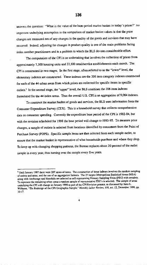
136
answ ers the question: "What is the value of the base-period market basket in today's prices?" An
important underlying assumption in the comparison of market basket values is that the price
changes are measured net of any changes in the quality of the goods and services that may have
occurred. Indeed, adjusting for changes in product quality is one of the main problems facing
index number practitioners and is a problem to which the BLS devotes considerable effort.
The computation of the CPI is an undertaking that involves the collection of prices from
approximately 7,300 housing units and 22,500 retail/service establishments each month. The
CPI is constructed in two stages. In the first stage, often referred to as the "lower" level, the
elementary indexes are constructed. These indexes are the 206 item category indexes constructed
for each of the 44 urban areas from which prices are collected for specific items in specific
outlets.' In the second stage, the "upper" level, the BLS combines the 206 item indexes
formulated for the 44 index areas. Thus the overall U.S. CPI is an aggregation of 9,064 indexes.
To construct the market basket of goods and services, the BLS uses information from the
Consumer Expenditure Survey (CEX). This is a household survey that collects comprehensive
data on consumer spending. Currently the expenditure base period of the CPI is 1982-84, but
with the revision scheduled for 1998 the base period will change to 1993-95. To measure price
changes, a sample of outlets is selected from locations identified by consumers from the Point of
Purchase Survey (POPS). Specific sample items are then selected from each sample outlet, to
ensure that the market basket is representative of what households purchase and where they shop.
To keep up with changing shopping pattems, the Bureau replaces about 20 percent of the outlet
sample in every year, thus turning over the sample every five years.
5 Until January 1997 there were 207 strata of items. The construction of these indexes involves the random sampling
of outlets and areas, and the use of an aggregation formula. The 27 largest Metropolitan Statistical Areas (MSA)along with Anchorage and Honolulu are selected as self-representing Primary Sampling Units (P5s) with cenainty.To represent the remaining urban areas a random sample of representative PSU's is selected. The sample of areas
underlying the CPI will change in January 1998 as part of the CPI Revision process, as discussed by Janet L.
Williams, 'The Redesign of the CPI Geographic Sample,' Monthly Labor Review. 119, no. 12, December 1996, pp.
10-17.
4

137
The CPI is used for many purposes, but measurement of changes in the cost of living is
one of the most important of these. The BLS has for many years used the concept of the cost-of-
living index as a framework for making decisions about the CPI and accepts the COLI as the
measurement objective for the index. 6 The cost-of-living index is a theoretical construct,
however, not a single or straightforward index formula readily amenable to practical use.
The cost-of-living index compares the cost to the consumer at different points in time of
maintaining a constant standard of well-being, without restrictions on the market basket. It is a
theoretical concept based on the well-being of the individual consumer, so that additional
assumptions about how to apply it as a nieasurement objective for an aggregated set of
consumers (such as the U.S. urban population) must be made. In addition, for an aggregate
measure, assumptions must be made about the implications of the distribution of prices paid for
the same good across markets. The general cost-of-living theory does not prescribe how any
compensation for changes in well-being would or should be administered. Thus, while the CPI
may be described formally in the context of a cost-of-living index, there is no single all-purpose
definition of this target. 7
In the most general sense, the cost-of-living index answers the following question: "What
is the minimum change in expenditure that would be required in order to leave a specified
consumer unit indifferent (or as well off) between a specified reference period's prices and a
comparison period's prices?"' The consumer's well-being depends on many aspects of life other
than market goods and services, e.g., environmental quality and amenities (such as clean air and
6 For a discussion of the relationship of tlhe CPI to th .*: : :i,,n index, see Roben Gillingham, "A ConceptualFramework for the Consumer Price Index," Procecr.L'- American Statistical Association 1974 Business andEconomic Statistics Section, (Washington, D.C.. An-,:-,. * ,ical Association, 1974).7 To some extent, the definition of a price index is . . : - the uses for which it is intended; see Jack E. Triplett,"Escalation Measures: What is the Answer? What. ::, -;'n ' in WE. Diewen and C. Montmarquette, eds.,Price Level Measurement: Proceedings from a Can,',, . ;- 'nsored by Statistics Canada (Ottawa, StatisticsCanada, 1983), pp. 457-87.' An alternative formulation of the cost-of-living ilid:: . :n :=:;ns of required income rather than expenditure. Thisformulation would imply the inclusion of income- and wage-based taxes. See, for example. Robert A. Pollak, "TheTreatment of Taxes in the Consumer Price Index," in The Thvaeon of the Cost-of-Living Index (New York, OxfordUniversity Press, 1989), pp. 193-199, and Roben Gillingham and John S Greenlees, "The Impact of Direct Taxes onthe Cost of Living," Journal of Political Economy, 95. no. 4. August 1987, pp. 775-796.
5

138
low crime), goods provided through taxes (such as national defense and fire protection), health
status. and future consumption goals (which depend on both current and expected future income.
and savings). All of these aspects of life can, and do, change over time along with commodity
and service prices. Most of these also are difficult to measure, and it would be even more
difficult to translate them into measured increments to well-being. The cost-of-living index
approximated by the CPI is a subindex of the all-encompassing cost-of-living concept,
specifically a subindex that is conditional on the excluded factors that affect consumer well
being, such as health status and the quantity and quality of govemment-provided goods and
services.9 The BLS defines the scope of the CPI to include only market goods and services or
govemment-provided goods for which explicit user charges are assessed.
In the case of medical care, for example, the CPI includes direct out-of-pocket
expenditures for medical care commodities and services, plus expenditures for the purchase of
health insurance. This definition includes the employee-paid share of premiums for employer-
provided health insurance coverage, as well as Medicare Part B monthly insurance premiums, but
excludes the portion of income and payroll tax payments used to fund the provision of medical
care for elderly and low-income beneficiaries. Although the advisory commission states that all
medical care spending should be included in the CPI, the BLS believes that the exclusion of
Medicaid and Medicare Part A is appropriate and consistent with the treatment of public schools
and other tax-funded goods, and services. '
Practical price index measures exist that do not hold the market basket of goods and
services fixed at its original value. Some of these index measures, known as "superlative"
indexes, have been shown theoretically to be closer to the cost-of-living concept than measures
9 See Pollak, Theory ofthe Cost-of-Living Index, and Gillingham, "A Conceptual Framework."'° U.S. Senate, Committee on Finance, Final Report, p. 37. The proper treatment of employer-provided medical care,
as well as other in-kind employee compensation, involves more difficult conceptual issues, and depends in part on
the uses made of the index. See Ralph Turvey et al., Consumer Price Indices: An ILO Manual (Geneva.
International Labour Office. 1989).
6
139
that track the cost of a fixed basket." The major superlative indexes are the Fisher and Tbmqv ist
measures. Using these formulas, one can construct an index that accounts for the changes that
consumers make in the quantities of the goods and services they consume in response to changes
in relative prices. By substituting goods that have become relatively cheaper for those that have
become relatively more expensive. consumers can achieve the same standard of well-being for
less than the cost of purchasing their original market basket. The difference between an index
that accurately accounts for this substitution and an index that does not (e.g. the Laspeyres index
used in the CPI) is known as substitution bias. Because the CPI holds the market basket fixed at
base period quantities, it incurs substitution bias by putting too much weight on the relatively
more expensive items from which consumers have shifted away. The superlative indexes,
because they adjust for changes in consumer expenditures, tend to avoid this type of bias. The
superlative indexes do, however, require estimation of the comparison period market basket.
Because it takes time to collect and process consumer expenditure data, a superlative index can
be produced only with a time lag.
III. Review of Advisory Commission Bias Estimates
Substitution Bias
The Commission report produces two estimates of substitution bias in the CPI: one for
the lower level of aggregation and one for the upper level of aggregation. At the lower level of
aggregation individual price quotes are aggregated to form subindexes for each category of
goods, such as apples, watches, or dental services. At the upper revel of aggregation these
"See W. E. Diewen. "Exact and Superlative Index Numbers," in Diewen and Nakamura, eds., Essays in IndexNumber Theory, Volume L, pp. 223-252.12 Whereas the BLS collects and processes CPI price data monthly, most CPI expenditure data are drawn from theCEX household interview survey, which is conducted quarterly. Fully edited expenditure data for a given year arenot available until late in the following year. As will be described in section VI] below, the BLS plans to take stepsto expedite the processing of the CEX data, but updating of expenditure weights on a monthly basis would beprohibitively expensive.
7

140
subindexes are collected into an all-items index. The formula currently used to aggregate the
individual price quotations to form the subindexes does not account for consumers' ability to
substitute across items within item categories when the relative prices of those items change-for
example, when the price of Delicious apples increases and the prsce of Granny Smith apples falls.
Similarly, the formula used to aggregate the subindexes to form the overall CPI does not reflect
the substitution across item categories that takes place when the relative prices of items in
different categories change-for example, when the price of apples falls relative to the price of
oranges.
For substitution bias at the upper level the commission's estimate of 0.15 percentage
point per year is based on BLS research that compares indexes calculated using superlative
formulas to an index calculated using the fixed-weight Laspeyres formula." The BLS and the
advisory commission essentially agree on the size and nature of the bias at this level.
Substitution bias at the lower level is sometimes confused with the separate problem of
formula bias." To understand what is meant by "formula bias," recall that the CPI measures the
change in the cost of purchasing goods and services using a formula that weights each item's
price by the quantity that was purchased during a base period. Because the household
'3 The original research was published in Ana M. Aizcorbe and Patrick C. Jackman, "The Commodity SubstitutionEffect in CPI Data, 1982-1991," Monthly Labor Review, 116, no. 12, December 1993, pp. 25-33. These estimates
subsequently have been updated by BLS staff. Until the introduction of the updated market basket in January 1998.the CPI may exceed the superlative indexes by somewhat more than this amount, as indicated by John S. Greenlees,"Expenditure Weight Updates and Measured Inflation," paper prepared for Third Meeting of the InternationalWorking Group on Price Indices, Voorburg, Netherlands, April 16-18. 1997 (Washington, D.C., Bureau of LaborStatistics); and Maithew D. Shapiro and David W. Wilcox, "Alternative Strategies for Aggregating Prices in the
CPI," paper presented at Federal Reserve Bank of St. Louis Fall Policy Conference on Measuring Inflation and RealGrowth. St. Louis, October 16-17, 1996 (University of Michigan).' For example, the commission is unclear about whether, in their usage, substitution bias equals, includes, or is
distinct from formula bias. At one point they state ". ..what we called 'formula bias' [we] now refer to as LowerLevel Substitution Bias" (see U.S. Senate, Committee on Finance, Final Reporr, p. 19). Subsequently, they state'BLS has reduced so-called formula bias, the part of Lower Level Substitution Bias resulting in substantial measure
from the introduction of sample rotation procedures" (p. 44). Then they state "Changing to geometric means will not
only solve the 'formula bias' problem.. .but will also alleviate the below-stratum-level substitution bias" (p. 51). Thelast of these statements, indicating that formula bias and substitution bias are distin:t phenomena, most closely
agrees with definition of formula bias that was given when it was originally identified by BLS research; see MarshallB. Reinsdorf, "Price Dispersion, Seller Substitution, and the U.S. CPI," BLS working paper 252 (Washington. D.C.,
Bureau of Labor Statistics, 1994). Appendix A of the present paper describes an additional confusion with thecommission's example of the related property of "time reversibility.'
8
141
expenditure surveys give information on dollar expenditures rather than quantities, the CPI
quantity %%eights must be derived indirectly. as expenditures divided by price. Until 1995
quantity weights for the items in the sample were formed by, first, projecting the initial price
collected for each item backwards using information on price trends for similar items, and, then,
dividing the appropriate expenditure figure by this backwards-projected price. This procedure,
however, had an unintended consequence. Items that were on sale as of the point in time when
they were first priced were systematically overweighted-expenditure divided by a low price
gives a high quantity weight. Because the prices of sale items are apt to rise in subsequent
months, this procedure imparted an upward bias, i.e., formula bias, to the index. The BLS
introduced procedures (principally what is known as "seasoning") to eliminate this formula bias
beginning in January 1995 for food-at-home and shelter, and June and July 1996 for all other
items.
To calculate the lower level substitution bias the commission first asserts that the
geometric means index is an unbiased estimate of the true cost-of-living index. They cite BLS
research showing from June 1992-December 1994 the difference between the growth rate of the
geometric means index and the CPI was 0.49 percentage point per year." Then the commission
makes an adjustment to take account for the changes made by the BLS during 1995 and 1996 to
eliminate formula bias, which the BLS has estimated to have reduced the rate of growth of the
CPI by 0.24 percentage point per year.i" Their estimate of lower level substitution bias therefore
is computed as the difference between 0.49 and 0.24, or 0.25 percentage point per year.
This estimate, however, may be too large. As described in Appendix A, the commission
fails to mention several strong assumptions about the distribution of price changes that they
5 The research paper cited by the commission is Brent R Moulton and Karin E. Smedley, "A Comparison ofEstimators for Elementary Aggregates of the CPI," paper presented at Western Economic Association Internationalconference, San Diego. July 7, 1995 (Washington, D.C., Bureau of Labor Statistics).6 See Roben McCletland, "Evaluating Formula Bias in Various Indexes Using Simulations," BLS working paper
289, 1996; and Brent R. Moulton, 'Estimation of Elementary Indexes of the Consumer Price Index," paper presentedat Amencan Statistical Association conference, Chicago, August 5. 1996 (Washington, D.C., Bureau of LaborStatistics).
9
142
implicitly use when claiming that the geometric means index is unbiased, or to note that, under
these same assumptions, the Laspeyres formula currently used by the BLS also is unbiased. There
is. moreover, reason to believe that the assumptions in question may not hold for many or most
of the CPI component strata. If they do not hold, the geometric means index still may be
unbiased, but only if the elasticity of substitution is exactly equal to one.'" If, on the other hand,
this elasticity is zero, the "seasoned" Laspeyres used by the BLS will correctly show price change
with no substitution.
As will be described in section IV, the BLS has made a commitment to evaluate the likely
applicability of the geometric mean aggregation formula this year, item category by item
category, and to make a decision by the end of the year about whether to adopt the geometric
mean approach to calculating some components of the CPI. It is unlikely that the conditions
necessary for the geometric mean formula to be unbiased will be found to hold in all cases.
Thus, the commission's estimate of lower level substitution bias may be too large.
New Outlet Bias
The comrtmission estimates that the entry of lower-priced outlets causes a bias of 0.1
percent per year. This estimate appears to be based on research conducted at the BLS by
Reinsdorf, which compared price levels in newly selected outlet samples with price levels in
outlet samples leaving the CPI." His estimates imply a price decline of about 0.25 percent a
year, which gives a figure of 0.1 percent per x.ir in an assumption that 40 percent of the CPI is
affected by new outlet bias.
7 The elasticity of substitution is a measure of consu,: -. .ii:mgness to substitute between commodities and isdefined by economists as the proportionate change e .. :'e quantites demanded divided by the proportionatechange of relative prices.' See Marshall Reinsdorf, nThe Effect of Outlet Price Ditferentials on the U.S. Consumer Price Index," in Murray F.Foss, Marilyn E. Manser and Allan H. Young, eds., Prnce Mcasurements and Their Uses, (Chicago, University ofChicago Press, 1993).
10

143
This estimate is subject to considerable uncertainty for three reasons. First, the effect of
outlet entry is likely to vary from year to year, and Reinsdorf's data cover only two years from
the late 1980's. Those years may be unrepresentative of long run trends. Second, Reinsdorf's
estimates have large enough standard errors so that conservative statistical hypothesis tests would
not rule out the hypothesis that the true effect of outlet changes is zero. Third, there is no
assurance that the item categories studied by Reinsdorf, food and gasoline, are representative of
other categories that may be subject to outlet bias.
Two additional considerations suggest that the estimate of 0.25 percent per year for the
items affected by new outlet bias is too high. First, this bias estimate is based on an assumption
that the new lower-priced outlets provide service of the same quality as the higher-priced
incumbents. In many discount and off-price stores reductions in costly retailer services help
make the low prices possible. (Examples of retailer services that might be less available at the
lower-priced outlets include knowledgeable sales staff, breadth and depth of product assortment,
assurance of item availability and quality, convenient location and hours, liberal return policy and
store ambiance.) Furthermore, under some circumstances, entry by low-priced outlets with
reduced services also could cause incumbents to reduce their services, thereby creating a
downward bias unless adjustments for these quality reductions were made in the CPI. Indeed,
because of the likelihood of quality declines, Reinsdorf interprets the 0.25 percent figure as an
upper bound estimate of outlet bias in those components of the index where such bias might
plausibly exist.
Second, changes other than entry of lower-priced outlets probably contribute to the price
declines in Reinsdorf's data. Since 1978, the BLS has updated its sample of brands and product
versions at the same time that it updates its outlet samples. Thus, if consumers were shifting
over time to cheaper brands or product versions, these choices would be reflected, through the
probability sampling methods used by the BLS, in selections of cheaper brands or product
versions in the newly sampled outlets, making their price advantage appear larger than it really is.
In a more recent study, Reinsdorf compares growth rates of sample average prices for food items
I1I
144
and CPI food indexes over periods from 1948 to 1963 and from 1967 to 1976, when the BLS
rarely changed the product version in the sample." These comparisons imply a price decline
from new outlets of just 0.1 percent per year, compared to the 0.25 percent estimate above. This
figure reflects price differences between outlets entering and leaving the sample because, for
most of those years, the BLS had a policy of allowing price differences between outlets to affect
its average price series but not its indexes.
Quality and New Products Bias
The largest share of the bias in the CPI that the commission concludes exists-0.6
percentage point per year, or more than half of the total of 1. I percentage points per year-arises
from an alleged failure to make adequate adjustment for changes in the quality of the goods and
services people buy and to account properly for the value to consumers of newly available goods.
Before commenting on the evidence marshaled by the commission in support of its
conclusions in the quality/new goods area, we emphasize that the BLS already has procedures in
place designed to account for changes in the quality of the items being priced. (It often
mistakenly has been assumed, though not by the commission, that the BLS makes few or no such
adjustments.) Although these adjustment procedures are not perfect, they do have a very
important effect on the rate of price change the BLS reports. The best available information on
this point applies to a CPI subindex covering roughly the commodities and services component
of the market basket (about 70 percent of the total, with shelter the largest exclusion). During
1995, this subindex would have risen by 3.9 percentage points had these procedures not been
applied. Because of their application, however, the subindex actually rose by only 2.2 percentage
points over the year. Roughly speaking, these figures imply that the adjustments made by the
9 Reinsdorf, "Price Dispersion."
12

145
BLS for changes in the quality of these goods and services amounted to 1.7 percentage points
over the course of a single year3.
The BLS also has established procedures for bringing new items into the index. The BLS
has updated the expenditure share information used to aggregate the CP! subindexes only once
every ten years or so, but the specific stores in which prices are collected and the specific items
priced are reselected on a five-year cycle. Although more frequent sample rotations undoubtedly
would be desirable, it is a fact that the BLS, by replacing 20 percent of the sample each year
through the POPS and the initiation of new samples of outlets and items, already devotes
considerable resources to ensuring that the sample of items priced is representative of what
consumers actually are purchasing.
The commission does not argue, of course, that the BLS is not making a good effort to
address quality/new goods biases, but rather that, in spite of a good effort, residual bias remains.
The report's approach to assessing this residual bias is to divide the CPI into 27 categories, and
then to make a judgment about the magnitude of the bias in each case. Unfortunately, the
evidence applicable to many of these categories is rather sparse.
Of the 27 categories, the commission assigns eight a quality/new goods bias of zero
(fuels, housekeeping supplies, housekeeping services, other private transportation, public
transportation, health insurance, entertainment services, and tobacco). Each of the remaining 19
categories is assigned an estimated bias, in all cases positive (i.e., they concluded that price
change is overstated because quality change is understated or the value of new products ignored).
The commission supported its estimates of bias using three types of evidence: first, analysis of
published and unpublished studies of quality/new goods bias for particular goods, second,
° See Brent R. Moulton and Karin E Moses. "Addressing the Quality Change Issue in the Consumer Price !ndex.forthcoming in Brookings Papers on Economic 4ctiviiy 1997:1 (Washington. D.C., Bureau of Labor Statistics.1997). These figures are somewhat different from those reported in an earlier version of theirpaper. They refinedtheir prior estimates principally to exclude some 'quality adjustments" that are made to account for simple changesin units of measurement or package size.
13

146
quantitative evidence assembled by the commission from independent sources of data, and third.
in the absence of direct evidence, estimates based on the judgment of the members.
For nine of the 19 categories (food at home other than produce, fresh fruits and
vegetables, food away from home, alcoholic beverages, other utilities including telephone, other
house furnishings, motor fuel, nonprescription drugs and medical supplies, and personal and
educational expenses), absent evidence, the commission is forced to fall back on its best
judgment. The alleged bias in these categories accounts for 0.11 of the 0.61 percentage point bias
the commission attributes to quality/new goods problems. The food and beverages categories are
an example; the commission's estimates of upward biases in these categories rest exclusively on
judgments regarding the value to consumers of increased variety on grocery and liquor store
shelves, together with the value of greater choice in restaurants, as shown in the following
quotation from the report:2
"...there is little if any published evidence on the food category, other than [Jerry]
Hausman's ... attempt to establish the value for the introduction of a new variety
of breakfast cereal... How much would a consumer pay to have the privilege of
choosing from the variety of items available in today's supermarket instead of
being constrained to the much more limited variety available 30 years ago? A
conservative estimate of the value of extra variety and convenience might be 10
percent for food consumed at home other than produce, 20 percent for produce
where the increased variety in winter (as well as summer farmers' markets) has
been so notable, and 5 percent for alcoholic beverages where imported beer,
microbreweries, and a greatly improved distribution of imported wines from all
over the world have improved the standard of living."
21 US. Senate, Comnmitee on Finance, Final Report, p. 28.
14
147
In putting forward these estimates. the commission does not cite any published or
unpublished studies, and indeed they comment on the absence of such evidence. Moreover, the
commission does not specify how their estimates were developed in the absence of evidence. In
several places the report characterizes the commission's specific estimates of bias as
"conservative," but it generally is not clear why this is believed to be so. The commission's
standard, the cost-of-living index, is defined as a function of consumer preferences, so reasonable
questions to ask are, "Whose preferences are being described?" and "How were they assessed?"
Although economists have methods for drawing inferences about preferences from market data
on observed consumer choices, the report does not indicate that the commission used such
methods in these cases. Appendix B presents an analysis of two categories, fresh fruits and
vegetables and motor fuel, which attempts to quantify the missed consumer benefit or "surplus"
that was described by the commission.' In both cases this analysis concludes that the
commission's estimates overstate the bias.
For four categories (shelter, apparel and upkeep, new vehicles, and used cars) members of
the commission have produced evidence that bears on the trend in prices for particular sorts of
items. The alleged bias in these categories accounts for 0.16 of the 0.61 percentage point bias the
commission attributes to quality/new goods problems. In each of these cases there are significant
problems with the inferences drawn by the commission.
An example of these problems is found in the commission's estimate of the quality bias
in the index for rent of shelter. The commission d reasoning is essentially as follows. Over the
period 1976 to 1993 the median rent increased jn m I percent per year faster than the CPI rent
index. This fact might suggest that the quali% - '&wnges already accounted for in the index are
substantial. According to the advisory cornon: En. however, these quality adjustments remain
inadequate because of a supposed 20 percent i:c;i:e in the average size of apartments between
l The analysis is taken from Moulton and Moses, "Addressing the Quality Change Issue."
15

148
1976 and 1993.23 In addition, they estimate that other improvements including "appliances,
central air conditioning, and improved bathroom plumbing, and other amenities" amount to 10
percent over the past 40 years, giving a net upward bias of 0.25 percent per year.
There are two fundamental problems with this analysis. First, rents generally increase
less than- proportionally to apartment size, which implies that the advisory commission's
proportional adjustment for apartment size would overstate the value of the increase. Second, the
commission's factual premise-the assertion that average apartment size has increased 20 percent
from 1976 to 1993-appears to be wrong. Although data giving an exact measure of the growth
in size of rental units since 1976 are not available, a recent study analyzing data from the
Residential Energy Consumption Survey, the American Housing Survey, and Current
Construction Reports concluded that the increase was probably about 6 percent-i.e., the
commission's estimate is too high by roughly a factor of three.2 ' After correcting this error, the
data cited by the commission no longer support an upward bias of the CPI rent index.
Another example is the commission's estimate that the growth in prices of new and used
cars has been overstated by 0.6 percentage point per year in the recent past. This estimate is
based on a flow of services approach in which the cost of consuming automobile services
declines as the useful life of the car increases. The commission presents data showing that the
average age of cars on the road has risen, which it takes as a measure of the increase in the useful
life of a car. To justify treating the increase in average age of cars as reflective of bias, the
commission also assumes that current CPI procedures do not capture any of the increases in
automobile durability that may have occurred. This latter assumption, however, is incorrect;
Appendix C lists some of the many durability-related model changes for which adjustments have
3 U.S. Senate, Committee on Finance, Final Report, p. 30. The commission provides no direct support for thisestimate, although reference is made to the changing characteristics of new single-family houses over the same
period. They also cite increases in the average number of bathrooms, and in the share of units containing central airconditioning, within the stock of rental units.2' Brent R. Moulton, "Issues in Measuring Price Changes for Rent of Shelter," unpublished paper presented at
Conference on Service Sector Productivity and the Productivity Paradox, Ottawa Canada, April 11-12, 1997(Washington, D.C., Bureau of Labor Statistics).
16

149
been made in the CPI over the past few years. Like other automobile quality adjustments in the
CPI. these are derived from manufacturer cost data, marked up to retail values. The commission
provides no evidence that this adjustment procedure would lead to an underestimate of the value
of quality improvements that have contributed to enhanced durability.
Finally, the commission's estimate that the CPI has overstated the rate of growth of
apparel prices by 1.0 percentage point per year since 1985 rests on a comparison of the official
CPI data with price indexes constructed using Sears catalogue prices for items whose
characteristics remain unchanged from one year to the next. Clearly one ought to have
reservations about drawing any general conclusions based upon the prices charged by a single
catalogue merchant. Moreover, BLS research has shown that price changes often are timed to
coincide with changes in product characteristics, particularly in the apparel market segment
where changing fashion is so important.' To the extent that this is true, the commission's
reliance on the data for unchanging items is likely to result in a downward bias, vitiating its
criticism of the CPI apparel index.
For the six remaining categories (appliances including electronic, prescription drugs,
professional medical services, hospital and related services, entertainment commodities, and
personal care) the advisory commission reviewed existing studies of bias in the price trends for
specific items to draw inferences about likely bias in the price trends for unstudied related items
within the category. These six categories can be categorized as constituting two major areas of
the index: medical care and high-tech consumer goods. More than half (0.34 percentage point)
2' See Jack E. Triplett, "Quality Bias in Price Indexes and New Methods of Quality Measurement," in Zvi Griliches,ed., Price Indexes and Quality Change: Studies in New Methods of Measurement, (Cambridge, MA, HarvardUniversity Press, 1971); Paul A. Arnknecht, "Quality Adjustment in the CPI and Methods to Improve It," inAmerican Statistical Association 1984 Proceedings of the Business and Economic Statistics Section (Washington.D.C., American Statistical Association, 1984); Paul A. Arnnknecht and Donald Weyback, "Adjustments for QualityChange in the U.S. Consumer Price Index, Journal of Official Statistics 5. 1989, pp. 107-23; Paul R. Liegey. Jr.,"Adjusting Apparel indexes in the Consumer Price Index for Quality Differences," in Murray F. Foss, Marilyn E.Manser, and Allan H. Young, eds.. Price Measurements and Their Uses. (Chicago, University of Chicago Press.1993); Paul R. Liegey, Jr., "Apparel Price Indexes: Effects of Hedonic Adjusument," Monthly Labor Review 117,May 1994, pp. 38-45; Marshall B. Reinsdorf, Paul Liegey, and Kenneth Stewart, "New Ways of Handling QualityChange in the U.S. Consumer Price Index," BLS working paper no. 276 (Washington, D.C., Bureau of LaborStatistics. 1995); and Moulton and Moses, "Addressing the Quality Change Issue."
17

150
of the quality/new goods bias the commission believes exists in the overall CPI is judged to
occur in just these areas of the index. These clearly are components of the index in which the
BLS faces particularly difficult measurement problems, though the inferences that the
commission has drawn about the magnitude of any bias in these index components involves
some degree of speculation and extrapolation.
The advisory commission's estimate of bias in the medical care component of the index
appears to have been largely based on just two recent empirical studies, one of cataracts, the
other of heart attacks, which both identified large quality improvements that are missed in the
calculation of the CPI.' Although we acknowledge that there have been enormous
improvements in medical technology over time, we also note the heterogeneity of the medical
services category, which includes services as diverse as dentistry, eyeglasses and eye care,
psychological counseling, podiatry, chiropractic, and physical therapy. Thus we are not
convinced that the two conditions cited by the commission should be considered representative
with respect to the unmeasured quality advances in the treatment of all medical conditions.
In some cases quality bias in the medical care component of the index may have arisen as
a result of failure by the BLS to capture improvements in procedures that led to shorter hospital
stays and out-patient treatment. The BLS recently has taken steps that, at least in principle,
should address medical care quality improvements of this type. For hospital services, beginning
in January 1997 the CPI has adopted the practice that previously had been used in the Producer
Price Index (PPI) of pricing completed treatments (as represented by the service bundles on
selected patient bills) rather than individual medical inputs. This change should permit BLS staff
to track changes in treatment over time.' This change, however, will not resolve all quality
2` The studies cited by the commission are Matthew D. Shapiro and David W. Wilcox. "Mismeasurement in the
Consumer Price Index: An Evaluation," in Ben S. Bemanke and Julio 1. Rotemberg, eds.. NBER Macroeconomics
Annual 1996, (MIT Press, 1996): and David M. Cutler, Mark McClellan, Joseph P. Newhouse, and Dahlia Remler,
Are Medical Prices Declining?" NBER working paper no. 5750 (Cambridge. MA, National Bureau of Economic
Research, 1996). The latter study, of heart attacks, was supported in part by the BLS.
See Elaine M. Cardenas, "Revision of the CPI Hospital Services Component." Monthly Labor Review, vol. I 19.
no. 12. December 1996, pp. 40-48.
18

151
adjustment problems in the medical care component. Some kinds of quality change are difficult
to evaluate. involving changes in patient outcomes, such as improved mortality or reduction in
pain. The BLS is continuing to support and encourage research on this topic, but we are
skeptical that it will be possible to develop methods that will permit reliable evaluation of all
kinds of quality changes on an on-going basis within the monthly CPI.
The area of high-tech consumer goods (e.g., consumer electronics) is one for which there
are a number of published studies documenting systematic quality bias of the CPI. Most of these
studies are based on the method of "hedonic" quality adjustment (i.e., adjustments based upon
the empirical relationship between the prices of various items and their characteristics), with
studies having been conducted of personal computers, television, video equipment, etc. The BLS
is currently applying hedonic methods in the PPI for personal computers and peripherals.
Projects are underway at the BLS to develop hedonic quality adjustment methods and improved
sampling of new products within the appliance category of the CPI.
In addition to these specific comments about the nature of the evidence on quality/new
goods biases assembled by the commission, there are several general remarks to be made. The
commission's estimates of bias are made case by case using a variety of methods, without any
clear statement of what methods are appropriately used in each circumstance. The absence of a
well defined methodology for deriving the commission's estimates represents a fundamental
reason why the BLS reaction to the quality/new products section of the report has been skeptical.
Also, in general, the commission's discussion of quality/new goods biases does not include
explicit recommendations regarding the adoption of procedures to correct the problems it
believes exist. In part, this appears to reflect a lack of consensus among economists about what
is practical and theoretically justified for measuring the benefit to consumers from new
products."s For production of the CPI and other national statistics the BLS must use methods that
are objective, reproducible, and verifiable.
- For examples of some of the methods that have been proposed, see the papers in Timothy F. Bresnahan and RobertJ. Gordon. eds., The Economics ofiVew Goods. (Chicago. University of Chicago Press, 1997).
19

152
The commission also failed to make any systematic effort to explore the possible
existence of negative biases in the CPI. Other analysts have hypothesized reduceu convenience
and comfort of air travel and deteriorating quality of higher education as examples of quality
decreases that are ignored in the CPI. More generally, whereas the commission notes some
service quality improvements, such as the introduction of automatic credit-card readers at
gasoline pumps, the BLS often hears complaints about broad-ranging declines in the quality of
customer service, which are equally difficult to incorporate in the CPI.
A more subtle issue is that price increases for many goods occur intermittently and often
are timed to coincide with model replacements or other quality improvements. The BLS
commonly adjusts for quality differences between successive models by, in effect, treating the
difference in price between them as wholly attributable to a difference in quality. There is a risk
that this procedure may over-adjust for quality change, imparting a downward bias to the index.
Methods have been introduced to try to minimize that possibility, but the commission paid little
attention to this potential problem.
From a BLS perspective, the most important question about possible quality/new goods
problems is what we might do to improve our procedures and ameliorate those problems.
Recognizing the particular difficulties associated with measuring medical care prices and high-
tech consumer goods prices, the BLS has devised and announced important improvements in our
methods. These include the changes noted above in our hospital price measurement procedures,
and prospective changes in our sample rotation 'rocedures that will allow us to update item
samples in rapidly changing market segments rmore frequently than once every five years (at the
cost of less frequent updates in more static nmrket egrments). In addition, the President's 1998
budget includes funds to improve the accurate.. :nethness. and relevance of the consumer price
data available from the BLS. The FY 199S bu. -ct request, if approved, would allow us to make
important progress in the quality/new goods area. by supporting greater use of hedonic
techniques and implementation of more aggressive procedures for identifying and beginning to
price new goods promptly once they appear in the marketplace.
20

153
IV. Short Run Recommendations'
Recommendation i. The BLS should establish a cost of living index (COLI) as its objective in
measuring consumer prices.
The advisory commission's report begins with one overarching recommendation: "The
BLS should establish a cost of living index (COLI) as its objective in measuring consumer
prices." The BLS basically concurs with this; indeed, the BLS long has said that it operates
within a cost-of-living framework in producing the CPI. That framework has guided, and will
continue to guide, operational decisions about the construction of the index. I Putting things
slightly differently, if the BLS staff or other technical experts knew how to produce a true cost-
of-living index on a monthly production schedule, that would be what we would produce. While
the BLS has no fundamental disagreement with the commission about what the objective of our
CPI program ought to be, we disagree to some extent about what changes to the index would be
feasible and prudent and about the timetable on which those changes could be implemented.
Because the cost-of-living concept does not imply a single all-purpose cost-of-living
index, the BLS will continue to need to make choices about the specific issues of formula,
coverage, and index construction. The BLS will continue to describe the scope and theoretical
assumptions of its price measures, as well as any necessary caveats with respect to their use.
Recommendation ii. The BLS should develop and publish two indexes: one published monthly
and one published and updated annually and revised historically.
Recommendation iii. The timely, monthly index should continue to be called the CPI and should
move toward a COLI concept by adopting a "superlative " indexformula to accountfor
29 The advisory commission uses two different methods for numbering their recommendations. See U.S. Senate.Committee on Finance, Final Report. pp. 2-3 and pp. 49-55. Herein we follow the numbers and text from pp. 2-3.30 BLS Handbook of Methods, Bulletin 2490, 1997, p. 170.
21
154
changing market baskets, abandoning the pretense of sustaining the fixed-weigki Laspeyres
formula.
Recommendation iv. The new annual COL index would use a compatible "superlative-index"
formula and reflect subsequent data, updated weights, and the introduction of new goods (with
their history extended backward).
Because these three recommendations address methods for dealing with the upper-level
substitution bias problem, we will discuss them together. The commission recommends that the
BLS should move to a "trailing Tornquist" formula for the monthly index." The Final Report
did not explicitly define this formula, but based on subsequent discussions with commission
members, we interpret this to mean a geometric mean formula in which the weights are lagged
expenditure shares, the weights are regularly updated, and the indexes are chained. The
commission also recommends that the BLS develop a new annual index that is calculated using a
superlative formula and is subject to revision.
The BLS continues to investigate several experimental indexes that use a superlative
formula at the upper level of aggregation. These include formulas which, due to the need for
current expenditure data, create indexes that must be produced with a lag, as well as new
methods that may approximate the superlative formula and allow the production of indexes in a
L....ciy fashion.
While the method of calculating the current CPI could be changed to incorporate a
superlative formula, the CPI would then have to be produced with a lag. Moreover, the
expenditure data that are required to derive the weights for the superlative index are available
with sufficient precision to be used in calculating such an index only at annual intervals, and thus
would not support a true monthly CPL.
3' U.S. Senate, Committee on Finance, Final Report, p. 50.
22

155
The timeliness of the CPI might be maintained by using some form of an approximation
to a superlative index. The commission's proposed "trailing Tomquist" formula, however, has
been shown to produce price changes that systematically understate the increases in the cost of
living, as measured by the superlative formulas."2 More recently, other approximation strategies
have been proposed, including a method based on the "constant elasticity of substitution" (CES)
formula." But such an approximation would not track the superlative indexes precisely-during
some years an index based on an approximation would rise more than the superlative index,
during other years it would rise less. This feature raises the issue of whether such an index
subsequently would need to be revised once the data were available to calculate the superlative
index. Another issue that needs to be addressed in considering use of approximations is the issue
of estimating the subaggregate indexes, i.e., the indexes for intermediate levels of aggregation,
such as for "food" or "transportation." Some of these indexes may consist of item categories that
are relatively close substitutes-fresh fruits, for example, consists of apples, bananas, oranges,
etc.-whereas others may consist of item categories that probably are not close substitutes-
medical professional services, for example, includes physicians, dentists, and eyecare. Because
the CES function is based on a single elasticity parameter which is assumed to be the same for all
items, while consumers' willingness to substitute is likely to vary across categories of items,
further research is needed to determine whether a simple approximation such as the CES would
produce sensible approximations for all of these subaggregates. Also, the use of an index based
on statistical approximation might be difficult to interpret and explain to users of the data. We
believe we would gain little, and possibly do much damage to the credibility of our statistical
system, if we were to move hastily to adopt untested techniques for producing the official CPI.
3'2 See Ana M. Aizcorbe, Robert A. Cage, and Patrick C. Jackman, "Commodity Substitution Bias in LaspeyresIndexes: Analysis Using CPI Source Data for 1982-1994." paper presented at the Western Economic AssociationInternational Conference in San Francisco, July 1996 (Washington. D.C., Bureau of Labor Statisucs); and Shapiroand Wilcox, "Alternative Strategies.""' See Shapiro and Wilcox, "Alternative Strategies." The CES formula that they proposed was originally derived byP.J. Lloyd, "Substitution Effects and Biases in Nontrue Price Indices." American Economic Review, vol. 65, June1975, 301-13, and was suggested by BLS staff as a method for approximating a superlative index without currentexpenditure data.
23

156
The President's 1998 budget includes funds to improve the accuracy and timeliness of the
CPI. and an important part of this request will support the production of a superlative index,
produced to a greater degree of accuracy than is now possible. The BLS plans to begin
publishing this measure in early 2002. In the interim, the superlative measures we currently
produce can be used to estimate the magnitude of the upper level substitution bias in the CPI, and
indeed are the best measures currently available for this purpose.
Recommendation v. The BLS should change its procedurefor combining price quotations by
moving to geometric means at the elementary aggregates level.
To address lower-level substitution bias, the commission has suggested adoption of a
geometric mean formula for aggregating price quotations, a formula that has been under
investigation by the BLS over the past several years. As discussed above, the current CPI
formula does not allow for the potential substitution among items within a category, such as
between different varieties of apples, when the relative prices of those items change. The
proposed geometric mean formula is based on an alternative assumption, namely that consumers
substitute among items in such a way as to hold the share of their expenditures devoted to each
item constant. Although this assumption is not likely to hold exactly for any particular stratum,
the geometric mean formula should provide a close approximation to the exact cost-of-living
subindex in cases where the stratum consists of substitutes, such as different varieties of apples,
and the price elasticity of demand for each variety is fairly large. If the elasticity of substitution
is zero, then the fixed weight Laspeyres formula is the appropriate measure of the cost-of-living
subindex. Again this assumption is not likely to hold exactly, but the Laspeyres index should
provide a close approximation to the exact cost-of-living subindex in cases where the price
elasticity of demand for each variety is quite small. It may be more plausible to assume that
consumers substitute freely between, for example, types of apples or between brands of
24
157
television sets when their relative prices change than to assume similar substitutability between,
for example, types of prescription drugs.
The BLS has begun issuing a monthly experimental measure that is constructed using the
geometric mean formula in all index components, and will make a decision by the end of this
year as to which components of the official CPI should employ the geometric mean formula."
Scanner data, studies of substitutions between brands, and other information will be used to
assess the propensity of consumers to substitute across items within individual item categories as
the relative prices of those items change. The likely date for implementation of any changes
decided upon for the official CPI is with the release of January 1999 CPI data.
Our best estimate is that the use of the geometric mean formula in all CPI subindexes
would lower the growth rate of the index by approximately one-quarter of one percent per year.
Partial adoption of the geometric mean formula, which is more likely than a full adoption, would
be expected to have a downward impact of between zero and one-quarter of one percent per year,
depending on how many, and which, indexes use the new formula.
V. Intermediate Run Recommendations
Recommendation vi. The BLS should study the behav ior of the individual components of the
index to ascertain which components provide most information on the future longer-term
movements in the index and which items have rtfhcisations which are largely unrelated to the
total and emphasize theformer in its data colhc::, air z-tivites.
Sample resources for the CPI are alloc %t:: N een the two major price surveys,
commodities and services (C&S) and housing:i. ..Jing to the relative importance and
variability of the survey estimators for each Cm :x'm.t. while taking into account the relative
costs of each survey. The sample for the C&S component of the CPI was designed to allocate
3 See Bureau of Labor Statistics, The Experimental CPI using Geometric Means (CPI-U-XG)." (Washington. DC.,Bureau of Labor Statistics, April 10, 1997).
25

158
resources systematically among major item groups and sample cities. utilizing models to
minimize the sampling variance of estimated price change, as measured by the all-items (less
shelter). national CPI, subject to cost and sample coverage constraints. Solution allocations
among items, outlets, and cities thus strike a balance with respect to the contributions of
components of sampling variability by sample items, their relative importance with respect to the
total consumer budget, and the relative cost of data collection and processing, while keeping
within the cost and coverage constraints of the program. 3"
The commission's recommendation suggests that data collection activities should focus
on a different objective, namely to provide information on the future longer term movements of
individual prices or the index as a whole. Forecasting inflation is a widespread and important
use of the CPI, of course, but one that is conceptually distinct from the measurement of cost-of-
living changes. If prediction of future inflation, or the measurement of "inflationary pressure,"
were the measurement objective of the CP1, this might imply different choices with respect to the
formulas and weights used in construction of the index, as well as with respect to the allocation
of the sample. The commission, however, emphasizes the use of the CPI as a measure of past and
contemporaneous changes in the cost of living in choosing the index formulas and weights, on
the one hand, while emphasizing the uses of the CPI in forecasting future price movements in
determining the sample allocation, on the other. This appears to be an internally inconsistent
strategy.
The commission suggests that resources devoted to the sample for bananas, a perishable
fresh fruit whose price-change sampling variability has been estimated to be substantial, but
whose price fluctuations are "not systematically related to the underlying trend movements of the
CPI," would be better allocated to surgical treatments, consumer electronics, and communication
services.3 6 The potential for saving resources by reducing data collection of items like bananas is
3 See S.G. Leaver, W.H. Johnson, R.M. Baskin, S. Scarlett, and R. Morse, "Commodities and Services SampleRedesign for the 1998 Consumer Price index Revision. Proceedings of the Survey Research Methods Section,American Statistical Association, 1996. forthcoming.36 U.S Senate, Committee on Finance. Final Report, p. 51.
26
159
fairly limited because the marginal cost of collection and processing is quite small-the stores
are already being visited to collect other grocery items and very little analysis is required after
collection. Because the sample has been allocated to minimize the variance, a reallocation of
resources away from any item with a high sampling variance toward other items necessarily
would result in an increase in the variability of its index and the reliability of the all-items index
would be diminished.
Recommendation vii. The BLS should change the CPI sampling procedures to de-emphasize
geography, startingfirst with sampling the universe of commodities to be priced and then
deciding, commodity by commodity, what is the most efficient way to collect a representative
sample of pricesfrom which outlets, and only later turn to geographically clustered samplesfor
the economy of data collection.
Because geographical coverage impinges on many aspects of the CPI data collection and
index estimation process, the practical meaning of this recommendation is somewhat unclear. By
the same token, the importance of the geographic structure underlying the CPI makes it a
continuing subject of BLS research.
The statement that the BLS should decide commodity by commodity, what is the most
efficient way to collect a sample, has been and will continue to be the standard practice. In
several cases, for example, postage and used cars, the BLS currently collects data on a national
level. In most cases, however, it is not possible to select samples of specific items at the national
level because of the lack of a national list (orframe) of items to sample, together with the sales
volume information needed to determine the probabilities of selection. Moreover, if specific
items were selected nationally, there would not usually be a feasible way to determine whether a
selected item was, in fact, cared by any particular sample retail outlet. These considerations
have led the Bureau to do sampling locally, by first selecting the urban area, then the outlet, and
finally the specific item within the outlet. This method helps to ensure that the sample of items is
27

160
timely and representative. The BLS is currently investigating potential uses of point-of-sale
(scanner) data which are available from private vendors, and in the future it might be possible in
some cases for the BLS to use such data to draw national samples of iterrs.37
Recommendation viii. The BLS should investigate the impact of classification, that is item group
definition and structure, on the price indexes to improve the ability of the index tofully capture
item substitution.
As part of the 1998 CPI revision activities, the BLS has just completed a process of
modifying the item classification structure." The ability of the index to capture consumer
substitution was one of the prominent factors that was considered in developing the new item
classification. In putting together the item classification, the BLS "also tried to see that [the
strata] formed natural groups, as consumers would view them...For example, using the consumer
view, items within the same stratum should have some affinity, such as substitutes (butter and
margarine), or complements (washers and dryers)."3 9
The commission points to some examples which cross item boundaries, such as "on-line
news services which compete with newspapers, automobile purchases with leases, and drugs
with surgical procedures they replace" as examples for which direct price comparisons are
needed so that the full substitution effect can be measured.' The BLS is sympathetic to the
commission's concem, and will continue to work to improve the CPI item structure.41 It seems to
us, however, that no feasible item classification system would completely capture the current and
" See Ralph Bradley, Bill Cook, Sylvia G. Leaver, and Brent R. Moulton, 'An Overview of Research on PotentialUses of Scanner Data in the U.S. CPI," paper presented at the Third Meeting of the International Working Group onPrice Indices, Voorburg, Netherlands, April 16-18, 1997 (Washington, D.C., Bureau of Labor Statistics)." Walter Lane, "Changing the Item Structure of the Consumer Price Index." Monthly LaborReview vol. 119 no. 12.December 1996, 18-25." Lane, "Changing the Item Structure." p. 22.3 See U.S. Senate. Committee on Finance, Final Report, p. 52.
l The January 1997 consolidation of three CPI strata-hospital room. other inpatient services, and outpatientservices-into one hospital services stratum was designed in part to capture substitution among those three settingsfor treatment provision. The inclusion of new cars and new trucks in a single new vehicles stratum is an example of asimilar change taking place as part of the January 1998 introduction of the revised CPI market basket.
28

161
possible future developments in consumer substitution behavior. Nor does it seem to us that the
item classification system is necessarily the most significant impediment to measuring the effects
of these substitutions. The more fundamental issue is the need to develop systematic methods for
identifying the substitution and accounting for differences in quality between the substituted
items.
Recommendation ix. There are a number of additional conceptual issues that require attention.
The price of durables, such as cars, should be converted to a price of annual services, along the
same lines as the current treatment of the price of owner-occupied housing. Also, the treatment
of "insurance " should move to an ex-ante consumer price measure rather than the currently
used ex-post insurance profits based measure.
When the BLS adopted the rental equivalence approach to pricing housing services in
1983, BLS staff were aware that the same conceptual issues arise in the pricing of other
consumer durables. 2 In principle the CPI is intended to measure the cost of consuming goods
and services, and durable goods provide a flow of services over time rather than immediate
consumption. To implement a flow-of-services approach, however, requires information on
either rental equivalence or user cost of the durable asset. In the case of housing, the existence of
rental markets makes it relatively easy to implement the rental equivalence approach, while the
long life of housing assets and the likelihood of price appreciation made the standard asset price
approach uniquely problematic. During the mid-1980s, BLS researchers investigated the
potential use of automobile leasing data to price automotive services, but at that time concluded
that the leasing markets were not sufficiently developed to support a leasing equivalence
approach to index construction. Subsequently, automobile leasing has grown to the point that in
1998 an automobile leasing stratum will be added to the CPI market basket. Currently BLS
'2See "Changing the CPI Homeownership Method to Rental Equivalence,' CP1 Dezailed Report, Bureau of Labor
Satistics, January 1983, pp. 3-17.
29
41-721 97 - 7

162
researchers are reexamining the flow-of-services approach for automobiles. possibly using a
leasing equivalence methodology. For durables other than automobiles. the lack of widespread
rental markets as well as the lack of data needed for direct estimation of user cost suggest that the
flow of services approach may not be practicable. As explained in our discussion of the
commission's quality bias estimate for automobiles, we do not agree with the commission's
premise that failure to price a flow of services necessarily leads to systematic quality bias.
The commission recommends that the BLS move the CPI for insurance to an "ex ante
consumer price measure" from the currently used "ex post insurance profit based measure." The
current CPI for health insurance does not directly price policies purchased by consumers."
Instead, an indirect approach to measuring the price of a policy is used; the price is seen as
deriving from the services provided by the insurer and the value of benefits paid to providers of
health care. The BLS prices these two parts separately, obtaining from insurers information on
retained earnings to measure changes in the vaiue of the insurance service component, and using
the price indexes in the CPI medical care component to measure changes in the cost of the health
benefits paid to providers. It is possible that direct pricing of health insurance policies would
have the virtue of automatically reflecting cost-reducing innovations in the treatment of medical
problems (such as the substitution of less-costly outpatient procedures). The countervailing
difficulty, however, is that health insurance policies can increase or decrease in price due to
changes in coverage or in the characteristics of the covered populations, and these changes may
be very difficult to observe or adjust for in the index.
The current CPI approach was adopted :n 1964. Prior to that the CPI collected the price
of the most widely-sold community-rated Blue Cross/Blue Shield policy. That approach was
dropped, however, when it became evident h.ai the quality of the policies was changing in ways
for which it was difficult to adjust the polic% pri..e In 1984-85 the Bureau experimented with the
direct pricing of a sample of health insurance policies but the experiment was terminated because
'3 Automobile and tenants insurance policies are priced directly in the CPI.
30

163
it again proved too difficult to maintain constant quality and coverage of risk over time. The
BLS recognizes the importance of the health insurance price movements to consumers as well as
to policy makers and will continue to search for ways to overcome the obstacles to accurate
adjustment for changes in policy characteristics.'
Recommendation x. The BLS needs a permanent mechanismfor bringing outside infonnation,
expertise, and research results to it. At the request of the BLS, this group should be organized by
an independent public professional entity and would provide BLS an improved channel to access
professional and business opinion on statistical, economic, and current market issues.
The BLS already has in place many mechanisms for bringing in outside information,
expertise, and research results. Business and labor research advisory committees meet regularly
with BLS staff and management and have long been a source of outside information and
expertise. A price research division has been a part of the price index programs since 1965, and
much of the discussion of CPI bias has been based upon the results of research conducted by BLS
staff. BLS economists and statisticians regularly solicit opinions from outside researchers by
presenting research papers at conferences and submitting them for publication at peer reviewed
journals. Academic researchers are regularly invited to present their research findings to BLS
staff in seminars. The Bureau's ASA-NSF-BLS fellowship program brings in scholars for
extended on-site research projects. The BLS has funded research by academic economists when
research by experts was needed to solve difficult measurement problems."
The BLS agrees that continued input from outside researchers is useful, and is currently
studying the possibility of creating an academic advisory commission. In addition, the BLS is
interested in having outside researchers address the important measurement issues that it faces,
" For discussions of past BLS research on the direct pncing of health insurance policies, and on the user-cost andleasing-equivalence approaches to pricing of automobile services, see Paul A. Armknecht and Daniel H. Ginsburg."Improvements in Measuring Price Changes in Consumer Services: Past, Present, and Future," in Zvi Griliches. ed..Output Measurement in the Service Sectors, (Chicago, University of Chicago Press, 1992)." See, e.g., Pollak, Theory of the Cost-of-Living Index; and Cutler, et al., "Are Medical Prices Declining?"
31

164
and will provide researchers with access to research databases to the extent possible, while
meeting data confidentiality requirements.
VI. Longer Run Recommendations
Recommendation xi. The BLS should develop a research program to look beyond its current
"market basket"frameworkfor the CPL
This recommendation suggests that the BLS should develop research programs exploring
"quality of life" issues such as time-saving benefits of new medical procedures and new
communication devices, and changes in the social or natural environment caused by rising crime
or new diseases. Because these things clearly affect our standard of living, a complete
accounting of U.S. economic progress would include them.
We do, however, have a reservation about this recommendation. Implicit in this
recommendation is a suggestion that the BLS should adjust the CPI for these effects. We think
that valuing changes in time allocation or in the general social environment may require too
many subjective judgments to fumish an acceptable basis for adjusting the CPI. Furthermore,
arriving at a comprehensive measure of changes in the quality of life will be quite difficult, yet
making such adjustments in only a few selected cases could make the CPI less accurate if these
cases are not representative. Finally, it is unclear whether "quality of life" valuations really
belong in an index used for the escalation of payments and adjustment of tax parameters. For
example, the advisory commission suggests that the CPI rent index should have made a quality
adjustment for changes in climate as renters migrated to the south.' Such a quality-of-life
adjustment, however, is properly viewed as out of scope under the current definition of the CPI.'
Most of the uses of the CPI have evolved within the context of an index limited to market goods
*" U.S. Senate, Committee on Finance, Final Report. p. 30.
"7 The commission's discussion of the appearance of AIDS, however, suggests agreement with the idea that not all
changes in the quality of life ought to be reflected in the CPI (U.S. Senate, Committee on Finance, Final Report. p.
47).
32
165
and service,. and presumably the appropriate uses of an index that incorporated changes in crime
levels. disease incidence, or income tax rates would be somewhat different from the current uses
of the CPI.
Recommendation xii. BLS should investigate the ramifications of the embedded assumption of
price equilibrium and the implications of it sometimes not holding.
Any systematic method for distinguishing quality change from price change must be
based on some theoretical framework and set of assumptions. In most cases the BLS, like
academic economists who do research in this field, relies on one or another assumption about
price equilibnum. An equilibrium assumption underlies hedonic methods for quality adjustment,
for example, as well as the matched model price comparisons commonly used by the BLS."
Although virtually all systematic methods for quality adjustment are based to some extent on
assumptions about price equilibrium, the nature of the assumptions differs between methods. Of
the methods used for quality adjustment by BLS, two (the "overlap method" and the "link
method") are based on a particularly strict equilibrium assumption-that quality differences can
be inferred from the price differences between individual items."9 The hedonic method, in
contrast, allows for random deviations of prices from equilibrium values and may allow for
differences in rates of price change between items of different vintages.
The commission recommends that the BLS investigate the assumption of price
equilibrium that underlies certain quality adjustment and item substitution procedures. We agree
that reducing reliance upon this assumption can sometimes make the CPI more accurate,
6 See lack E. Triplen, "Concepts of Quality in Input and Output Price Measures: A Resolution of the User Value-Resource Cost Debate," in Murray F. Foss, ed., The U.S. National Income and Product Accounts: Selected Topics(Chicago. University of Chicago Press. 1983).' For discussion of the quality adjustment methods used by the BLS. see Paul A Annknecht, Walter F. Lane, andKenneth J. Siewart, "New Products and the U.S. Consumer Price Index," in Timothy F. Bresnahan and Roben 1.Gordon, eds.. The Economics of New Goods (Chicago, University of Chicago Press, 1997): Reinsdorf, Liegey, andStewart. "New ways of Handling Quality Change;" and Moulton and Moses. "Addressing the Quality ChangeIssue."
33
166
particularly for long run comparisons. Indeed, the BLS already has made considerable progress
in doing this. Recent tabulations indicate that item replacements adjusted for quality using the
methods that embody a strong price equilibrium assumption (i.e., the "overlap method" and the
"link method") declined from about 2 percent of prices collected in 1983 to 0.62 percent in
1995.5 In addition, the CPI for prescription drugs now reflects consumers' savings from buying
therapeutically equivalent generic substitutes for branded products. We plan to continue research
on avoiding bias from unwarranted price equilibrium assumptions.
Recommendation xiii The BLS will require a number of new data collection initiatives to make
some progress along these lines. Most important, data on detailed time use from a large sample
of consumers must be developed.
The final longer run recommendation is that the BLS should develop new data collection
initiatives on time use and "quality of life" issues. These data would support the research
programs described in the commission's first longer run recommendation. We agree that time
use data would be valuable to researchers, and we concur with the focus on using them for
supplementary indicators rather than as part of the main cost-of-living framework.
VIL. Conclusion
The advisory commission report has performed a service by calling to the attention of
policy makers the many and varied issues that the BLS faces in constructing the CPI. Most public
attention has been focused on the commission's estimates of CPI bias, but the central argument
of the report is that almost every assumption underlying the procedures used around the world for
price index construction is called into question by the pace and form of market developments.
The issues are not new to index number experts (many of the issues are discussed, for example,
" Moulton and Moses, "Addressing the Quality Change Issue," Table 4.
34
167
in the articles in the December 1993 Monthly Labor Review), but the quantitative and budgetary
importance of price measurement problems and techniques have not always been appreciated by
users.
As discussed earlier in this paper, the BLS has a vigorous program of research and
development activities aimed at improving the CPI. In one category are the activities related to
upper- and lower-level substitution bias. These include:
* The continued monthly publication of the experimental geometric mean index (the
CPI-U-XG) and the evaluation of the geometric mean formula for use in the CPI-U and
CPI-W, probably beginning in January 1999.
* The continuing annual publication of experimental superlative indexes, and (assuming
approval of the Bureau's associated budget requests) introduction of an official
superlative index as a supplement to the CPI-U and CPI-W in 2002. With the
development of the CPI-U-XG, the experimental superlative indexes can be constructed
and compared using individual category indexes based on both arithmetic and geometric
mean formulas.
* Introduction of a new CPI market basket in January 1998 based on 1993-95 consumer
expenditure pattems, and consideration of a more frequent schedule of market basket
updates than the roughly ten-year cycle followed in the past. The BLS FY 1998 budget
initiative also calls for development ot an enhanced processing system that will enable us
to construct expenditure weights that !.-:' iUStwo years old when introduced into the
index. (By contrast, the 1993-95 mark: >'.ket will be 3 1/2 years old when it is
introduced in January 1998.)
The advisory commission recommends mi-i: a geometric mean formula for upper-level
aggregation, and annual market basket updaie. to approximate a superlative index while
avoiding the need for index lags or revisions. Evidence indicates that such an index would be
downward-biased relative to a cost-of-living index. As recommended by Shapiro and Wilcox,
35

168
however. one could develop an index based on the CES formula that provides a close
approximation to a superlative index over some historical period. The BLS plans to estimate such
an index as part of its experimental superlative index program. Additional research is needed on
the approximation properties of the CES formula, especially below the U.S. allritems level,
before it-could be considered for use in the CPI-U or CPI-W. Moreover, a move away from the
arithmetic-mean Laspeyres formula above the category level could make the CPI more difficult
to use and explain, and these considerations would have to be weighed against the potential
advantages of a closer approximation to a cost-of-living index. Also weighing in would be the
potential disadvantages of using a formula based upon an approximation to a superlative index,
which might need to be revised once the data were available to calculate the superlative index.
This paper has emphasized that substitution bias, and especially upper level substitution
bias, accounts for a relatively small part of the total bias that the advisory commission argues
exists in the CPI. Quality change in existing goods and services, the introduction of new
products, the establishment of new outlets, and the disappearance of older products and outlets,
present extremely important issues for which there are, as yet, no general solutions. The absence
of general solutions explains why the commission has no short-run recommendations in these
areas. The BLS will continue to study the pertinent intermediate-run recommendations-use of
leasing equivalence for automobiles, direct pricing of health insurance, and investigation of
improved item classification structures-but these are unlikely to solve the fundamental
measurement problems even in specific CPI components. Finally, the absence of systematic,
well-accepted ways to deal with these problems also means that there are no rigorous ways to
measure the new outlet or quality/new goods biases potentially created in the CPI. The advisory
commission, like other observers, was forced to use introspective or extrapolation methods to
obtain many of their bias estimates.
The BLS specifically rejects several of the estimated quality or new goods biases, in cases
where the commission presented new evidence. Examples of these cases noted in Section III
above include the estimates of a 0.25 percentage point annual bias in shelter, a 1.0 percentage
36

169
point annual bias in apparel and upkeep. and 0.59 percentage point annual biases in new and used
cars. Together. these comprise 0.16 of the 0.6 total estimated quality/new goods bias in the
overall CPI. In addition, the evidence presented in Appendix B suggests that the commission's
estimates of bias for the food and motor fuel components likely are overstated. Most of the
remaining estimated bias comes from two areas of the index: medical care and high-tech
consumer goods. These clearly are components of the index that present particularly difficult
measurement problems, but the quantitative evidence is very fragmentary and the BLS is
reluctant to speculate as to what the magnitude of any bias in these index components might be.
Finally, some analysts have cited potentially countervailing declines in quality, particularly in
services, that are not reflected in the CPI or in the advisory commission's bias estimates.
For the BLS, the primary task is not to evaluate the bias estimates set forward by the
advisory commission or other groups, but rather to employ the most accurate methods available
for dealing with quality change and with new goods and outlets. Those methods must be
rigorous, objective and reproducible, minimizing the role of analyst judgment, although these
considerations make it very difficult to incorporate in the CPI the benefits of some types of
product innovation." Improvements in medical care that enable patients to lead more active lives
have undoubted value, for example, but that value cannot now be, and may never be, measured
objectively enough to be reflected in official data series. Notwithstanding such limitations, the
BLS is taking several steps to improve its methods for dealing with quality change and new
products:
* Effective in January 1997, two improvements were made in the hospital and related
services component of the CPI. The hospital room, other inpatient, and outpatient
subcomponents were consolidated to enable the index to reflect shifts in the mix and
importance of treatment. At the same time, there was a shift from pricing individual
Marin Feldstein, in testimony before the Senate Finance Committee (February It, 1997), has agreed that the CPImust be based on tested and reliable statistical methods, even though in his view the resulting estimate will overstatethe srue increase in the cost of living.
37

170
items (like units of blood) to pricing the collections of services on selected patient bills;
among the benefits of this change are a better reflection of alternative reimbursement
methods and an enhanced potential for quality adjustment.
* In 1999, the BLS will implement a change in the CPI's sample rotation procedures from a
city-based to an item-based sequence. This ultimately will make it possible to update
item samples in rapidly changing market segments more frequently than once every five
years (at the cost of less frequent updates in more static market segments).
* The BLS FY 1998 budget request calls for data collection to support greater use of
hedonic techniques that explicitly account for changes in the characteristics of items
being purchased. (Even in the absence of such funding, the use of hedonic regression for
quality adjustment likely will expand into product categories such as personal computers
and televisions.) The requested resources also would support implementation of more
aggressive product initiation procedures for identifying and beginning to price new goods
promptly once they appear in the marketplace.
* Other potential intermediate-term changes include the direct pricing of health insurance
policies and a leasing equivalence approach to pricing of automobile services, as
recommended by the advisory commission. Both approaches have been evaluated by the
BLS in the past and rejected as infeasible, but new developments in the leasing and
medical care markets argue for their continued consideration.
Unfortunately, the ongoing controversies surrounding cost-of-living measurement and,
more generally, appropriate federal indexation policy, have led much of the public to conclude
that the CPI is somehow "broken." Although the BLS rejects that notion, it is evident that the
expanding number of users of the CPI have objectives and priorities that sometimes can come
into conflict. When this happens, the result can be an index that is less than optimal for certain
purposes. One example mentioned above reflects the competing objectives of an index that is
free of upper-level substitution bias (as might be desired, for example, for benefit indexation),
38

171
and of one that is not subject to lags or routine revision (for example, for indexing debt
instruments. Some also have argued the need for specialized indexes for program beneficiaries
or other population subgroups. It is, in fact, commonplace to observe that there is no single best
measure of inflation. The BLS response to this situation has been to develop a "family of
indexes" approach, including experimental measures designed to answer different questions from
those answered by the CPI-U and CPI-W. This "family of indexes" now includes the CPI-U-XG,
the CPI-E corresponding to the market basket of elderly consumers, and the experimental
superlative measures, and under the BLS FY 1998 budget request will include a production-
quality superlative measure beginning in 2002. As mentioned above, an experimental CES index
is a likely addition to the group.
The BLS is engaged in numerous CPI program enhancements that have not been
mentioned above. Some are part of the six-year CPI revision program now underway:
conversion to computer-assisted data collection and a telephone-based POPS survey,
improvements to the housing sample and estimator, and enhancements to the CEX survey
processing system. In addition, the FY 1998 budget request, if approved, would support an
expansion in the CEX sample, permitting more accurate expenditure weights and a more timely
CPI market basket. The solutions to many CPI measurement issues, however, must await
methodological breakthroughs in economics, or improved availability of data. Unfortunately, the
techniques available for measuring the gains in consumer welfare from new products (and the
losses from product disappearances) are in their infancy, and may never be adaptable for
implementation in a large, ongoing price measurement program like the CPI. The increased use
of scanner data in U.S. consumer markets offers broader opportunities, and the BLS has been
engaged in a significant research effort to explore the many possible uses of these data, in
identification of new products and outlets, sampling of items, and ultimately in the computation
of the CPI itself.
In summary, the concluding statements of the BLS report to the House Budget Committee
in April 1995 remain applicable today. The BLS is intensely aware of the sensitive nature of the
39

172
data it produces, and of the critical need for these data to be as accurate as possible, It will
continue to Investigate the measurement issues that it and others have identified, and will
introduce corresponding improvements to the index as quickly as it can.
40
173
Appendix A. Technical Issues About Lou er Level Substitution Bias
This appendix describes two technical problems with the commission's discussion of
lower level substitution bias and formula bias. The first of these problems involves the
commission's discussion of "time reversibility."' The commission describes this property as a
"requirement or test for an index number...that the index should remain the same if the
underlying prices undergo a reversal." Their example of this property, however, is incorrect. In
their example, the quantity of beef is 1.0, and the price of beef starts at 1.0 in period 1, rises to
1.6 in period 2, and then falls back to 1.0 in period 3. The commission claims that in such a case
the CPI would add the 60 percent increase between periods I and 2 to the 37.5 percent decrease
between periods 2 and 3 to show a total increaqe of 22.5 percent between periods I and 3.
Adding the percentage changes, however, is contrary to any reasonable procedure and is not an
accurate description of current or past BLS methods. The ratio of the price of beef in period 2 to
its price in period I is 1.6, and the ratio of the price in period 3 to the price in period 2 is 0.625.
So in this case the CPI would multiply the relative changes (1.6 x 0.625 = 1), correctly showing
no change in price between periods I and 3. Thus it is inaccurate to attribute the bias shown in
this example to the CPI.
A second problem is the commission's assertion that the geometric mean formula would
eliminate lower level substitution bias. The commission states that the difference between a
geometric means index and a Laspeyres index "is an estimate of the bias of the Laspeyres
formula, since [Matthew] Shapiro and [David] Wilcox... have shown that the geometric mean
provides an unbiased estimate of the underlying cost-of-living index."' This statement is
surprising, because it is well known that the geometric mean i,,dex is unbiased only under
restrictive conditions. The basis for the commission stated view appears to be as follows:
U. S. Senate, Committee on Finance, Final Report ofthe Advisory Commission to Study the Consumer Price Index.Print 104-72, 104 Cong.. 2 sess. (Washington. D.C.. Government Printing Office. 1996). p. 17.: U.S Senate, Committee on Finance, Final Report, p. 42. The article cited in this quotation is Matthew D. Shapiroand David W. Wilcox, "Mismeasurement in the Consumer Price Index: An Evaluation." in Ben S Bernanke andJulio I Rotemberg, eds., ,VBER Macroeconomics Annual 1996, (MIT Press, 1996).
41

174
"Shapiro and Wilcox...have provided an elegant rationale for the geometric
approach based on the correlation of relative prices over time. Provided that this
correlation is small, a modification of the geometric mean is approximately
unbiased for the underlying cost of living index, and this characterization does not
require information about the underlying system of consumer's preferences" (U.S.
Senate, Committee on Finance, Final Report, p. 19).
This statement mischaracterizes the discussion in Shapiro and Wilcox. That article made several
important assumptions that are not mentioned by the commission, including assumptions about
consumers' preferences. These assumptions are stated by Shapiro and Wilcox when they describe
the results of BLS research:3
"Several recent papers [by BLS authors]...have explored another alternative to the
Laspeyres-based formula, namely the modified geometric means estimator...Under
the same assumptions as we used above (CES utility, stationary distribution of
relative prices, etc.), one can show that the modified geometric means estimator is
approximately unbiased for the true cost-of-living index" (Shapiro and Wilcox,
"Mismeasurement," p. 111).
The assumptions made by Shapiro and Wilcox are fairly restrictive. For example, the
assumption of a stationary distribution of relative prices is an assumption that all of the prices in
a stratum follow the same underlying trend. Prices in heterogeneous strata very likely violate this
assumption because dissimilar goods may well follow different trends. Prices even in relatively
3The BLS authors cited by Shapiro and Wilcox are Brent R. Moulton, "Basic Components of the CPI: Estimation of
Price Changes." Monthly Labor Review, 116. no. 12, December 1993; Marshall B. Reinsdorf and Brent R. Moulton.'The Construction of Basic Components of Cost-of-Living Indexes," in Timothy F. Bresnahan and Robert J.Gordon, eds.. The Economics of New Goods (Chicago, University of Chicago Press, 1997); and Brent R. Moultonand Karin E. Smedley, "A Comparison of Estimators for Elementary Aggregates of the CPI," paper presented atWestern Economic Association International conference, San Diego, CA, July 7, 1995 (Washington, D.C., Bureau ofLabor Statistics).
42

175
homogeneous strata, such as tomatoes, can violate this assumption if some goods are produced
with different technologies, such as hand-picked versus mechanically picked tomatoes.
Moreover, if all of these assumptions hold (stationarity, small correlation of relative
prices over time, CES utility), the seasoning method now used to estimate the CPI component
indexes also is unbiased. As Shapiro and Wilcox state, under their assumptions:
"If pI-,, (the autocorrelation of the relative prices between periods I and n) is
small, [the "seasoned" version of the CPI]...should provide quite an accurate
estimate of the rate of increase in the true cost-of-living subindex, regardless of
the elasticity of substitution" (Shapiro and Wilcox, "Mismeasurement," p. 110).
The fact that the growth rates of geometric means index and the seasoned index actually differ
implies that an assumption, probably stationarity, is being violated. This weakens the
commnission's argument that the geometric means index necessarily approximates a true cost-of-
living index and points to the importance of taking account of consumer substitution behavior. If
relative prices are not stationary, then the geometric mean formula may still be the exact measure
of the stratum cost-of-living subindex, but only if the elasticity of substitution equals one.'
Altematively, the seasoned Laspeyres formula may still be the exact measure of the stratum cost-
of-living subindex, but only if the elasticity of substitution equals zero. The BLS intends to
determine which of these assumptions provides the closest approximation, item category by item
category.
' Shapiro and Wilcox, "Mismeasurement," fn. 22. p. II1.
43

176
Appendix B. Critique of Advisory Commission's Bias Estimates for Fresh Fruits and,
Vegetables and Motor Fuel'
Freshfruits and vegetables.
The quote cited above [see section III] indicates that the advisory commission attributes a
bias of 20 percent over the period 1967-96 due to increased seasonal availability and variety. It
is reasonable to think that, to the extent that consumers value the increased seasonal availability
of produce, they will consume more of it. Our analytical framework is to consider the
"November strawberry" to be a new good, distinct from the "June strawberry," and measure the
consumer surplus associated with the new good.2
Among the various methods that have been proposed for incorporating new goods in a
cost-of-living index, Jerry Hausman's suggestion of calculating the consumer surplus from a
linearized demand curve is particularly easy to apply to back of the envelope calculations.'
Hausman's linearized method implies that the percentage bias of the price index from failure to
incorporate the consumer surplus from a new good, n, is approximately
(1) bias=-0SxSS. / n
where Sn is the percentage expenditure share of the new good after introduction and o3n is its
price elasticity of demand. Thus the calculation of consumer surplus and bias can be inferred
' This appendix is an excerpt from a study by BLS researchers: Brent R. Moulton and Karin E. Moses, "Addressingthe Quality Change Issue in the Consumer Price Index,. forthcoming in Brookings Papers on Economic Activity
1997:1 (Washington, D.C., Bureau of Labor Statistics, 1997).2 See W. Erwin Diewert, "The Treatment of Seasonality in a Cost-of-living Index," in W.E. Diewert and C.Montmarquette, eds., Price Level Measurement: Proceedingsfrom a Conference Sponsored by Statistics Canada
(Ottawa. Siatistics Canada, 1983).3 See Jerry Hausman, "Cellular Telephone. New Products and the CPI," unpublished paper (Massachusetts Instituteof Technology. 1997). Hausman refers to his linearized method as a "lower bound" on the consumer surplus, but it isunclear to us whether the conditions for the method to be a lower bound-a convex shaped demand curve-necessarily hold in all cases.
44

177
from information on the expenditure share, which is often readily available, and the elasticity of
demand. which can be estimated or inferred from elasticity estimates for similar Poods. I
New varieties or seasonal availability of fresh fruits and vegetables face many substitutes,
not only from other fresh produce, but also from frozen fruits and vegetables. We assume a value
of-l.0 for J.n Under these assumptions, equation I implies that the increased consumption of
new seasonal items and varieties as a share of current consumption would need to be quite
large-about 40 percent of 1996 expenditures-to be consistent with the advisory commission's
estimated index bias of 20 percent.5
Table B I presents U.S. Department of Agriculture data on changes in per capita
consumption of fresh fruit from 1975 to 1995. The change in consumption is shown, somewhat
unconventionally, as a percentage of 1995 consumption, because the shares in equation 1 refer to
current period consumption. As the advisory commission observes, per capita consumption of
many fruits has indeed increased substantially over this period: in particular, limes, cranberries,
grapes, kiwifruit, mangos, papayas, and strawberries. Despite these large increases, however,
most of these items continue to represent a small percentage of overall fruit consumption, so that
the total increase in per capita fruit consumption as a share of 1995 consumption is only 14
percent (measured in pounds). The largest absolute increase in consumption of fruit is that for
bananas. We are confident there was no important improvement in seasonal availability of
bananas and that there were only minor increase :m consumption of new varieties of bananas
over this period. In addition, consumption ofr .:': '. Jid not change significantly and
consumption of oranges decreased. We wop.d- x:.. her the use of apples for baking may have
decreased during this period, which might nma- >sble increase in the consumption of raw
apples.
' If a new variety fully replaces an old one, the consumer iurplus calculation should deduct the lost surplus of thedisappearing variety from the surplus gained from ihe ne aritty.
Ideally, one would examine monthly consumption data to isolate seasonal changes in consumption, but such data donot appear to be available.
45

178
We do not attempt to calculate the overall bias using equation I because doing so would
require average price or expenditure data for each of the detailed categories, which we have not
been able to assemble. As mentioned earlier, under Hausman's model and our earlier
assumptions, to be consistent with the commission's bias estimate consumption of new varieties
and seasonal items would need to increase by about 40 percent over thirty years, which
annualizes to 25 percent over the twenty years for which we have data. If increased consumption
of seasonal varieties was relatively unimportant for apples, bananas, and citrus fruits, which,
according to the Consumer Expenditure Survey of the Bureau of Labor Statistics, together
represent 61 percent of dollar expenditures on fresh fruit in 1995, it would be difficult for
increased seasonal consumption of the other fruits to produce an estimated bias as large as the
commission proposes.
Table B2 shows changes in consumption of vegetables from 1972 to 1995. Unlike the
data for fruit, the data for vegetables show important increases in consumption for many items
and thus appear, at first glance, to be consistent with the advisory commission's estimates of
bias. Under the assumptions stated above, our consumer surplus calculations indicate that for the
commission's estimate to hold, the growth in consumption over thirty years would need to be
about 40 percent of current consumption, which annualizes to 29 percent over the twenty-three
years for which we have consumption data. This is, in fact, very close to the overall increase
over this period: 27 percent. We are skeptical, however, about concluding that the increase in
consumption derives entirely from improved seasonal availability. A BLS food specialist, Bill
Cook, has suggested that the increase in seasonal availability of fresh vegetables mostly occurred
before 1985, as evidenced by a 1984 internal BLS study showing that 91 percent of the CPI price
quotes for the "other fresh vegetables" category were by then available year round.6 Table B2
shows, however, that almost half of the increase in consumption of fresh vegetables occurred
6 Internal memorandum from William L. Weber to Dan Ginsburg, U.S. Bureau of Labor Statistics, May 25, 1984.
46

179
after 1985. Part of the increase appears to have been driven by shifts in preferences, perhaps as a
response to improved knowledge about the health benefits of fresh vegetables.
Motorfuel
For the motor fuel category, the advisory commission attributes "a small upward bias of
0.25 percent per year to the CPI for ignoring the convenience and time-saving contribution of
automatic credit-card readers built into gasoline pumps."' Because the commission applies this
estimate over a ten-year period, the estimate of the cumulative bias from this source amounts to
2.5 percent.! Our approach to measuring the consumer surplus created by pay-at-the-pump credit
card technology is to attempt to value the saving in time. Suppose that paying at the pump saves
two minutes per fill-up, and that the customer's time is valued at $18 per hour (average total
compensation per hour for all workers in private industry was S17.49 in 1996). Then the value of
paying at the pump is 60 cents per fill-up. Assuming that ten gallons are purchased, the quality
bias for the customer who pays at the pump is 6 cents per gallon, or roughly 4.5 percent of the
cost of a gallon of gasoline.
Since this service is of value only to the customers who use it, one must next determine
the approximate percentage of gasoline purchasers who use pay-at-the-pump technology.
Although we have not found direct information on this percentage, the September 1996 issue of
the trade joumal National Petroleum News reports that 28 percent of the retail facilities operated
by thirteen oil companies had installed pay-at-the-pump technology as of 1996.9 Since many of
U.S. Senate, Committee on Finance, Final Report of the Advisory Commission to Study the Consumer Price Index.Print 104-72. 104 Cong., 2 sess. (Washington, D.C., Government Printing Office, 1996), p. 36.
We also note that the report does not address possible unmeasured decline in retail services, such as theintroduction of fees for providing air for tires at some service stations. In addition, the advisory commissionincorrectly assumes that the CPI does not make quality adjustments for air pollution mandates and, agreeing with thissupposed BLS practice, makes no bias adjustment for the mandates itself Since BLS does, in fact, make cost-basedadjustments for motor fuel pollution mandates, the commission presumably should have counted these as downwardbias (see U.S. Bureau of Labor Statistics, "Quality Adjustment for Gasoline," CPl Detailed Report. January 1995. p.8)."'Pay-at-the-Pump Shows Solid Growth in '90s.' Nationat Petroteum News. September 1996, p. 22.
47

180
the customers at these stations do not use credit cards, we attempt to find the percentage of
gasoline customers who do so. We have not found published information, but an industry source
has told us that roughly 35 percent of sales are made through credit cards.
A naive estimate of the proportion of sales using pay-at-the-pump technology would thus
be 10 percent (28 percent x 35 percent). However, there are at least three reasons why this
estimate is too low: first, pay-at-the-pump technology was doubtless first targeted at high-
volume sites in areas with high credit card usage; second, the availability of the technology
induces customers to make more use of credit cards; and third, the technology is spreading
rapidly, so that even estimates published in September 1996 will understate current availability.
Consequently we take 25 percent as our estimate of the percentage of customer sales made with
pay-at-the-pump technology at the end of 1996. Under these assumptions, we calculate the
cumulative index bias from neglecting the benefits of this technology as approximately 1.1
percent (4.5 percent x 25 percent), which is less than half of the advisory commission's estimate.
48

181
Table Bi. Per Capita Consumption of Fresh Fruits, by Type, 1975-9SUnits as indicated
Cianee. 1975-95Pounds Per capita As percentage of In
Type offruit 1975 1985 1995 1995 consumption poundsCitrusOranges and temples 15.9 11.6 12.3 -29.6 -3.6Tangerines and tangelos 2.6 1.5 2.0 -27.9 -0.6Lemons - 2.0 2.3 2.9 32.1 0.9Limes 0.2 0.6 1.2 81.7 1.0Grapefruit 8.4 5.5 6.0 -38.4 -2.3
Total 29.0 21.5 24.4 -18.9 -4.6
NoncitrusApples 19.5 17.3 18.9 -3.0 -0.6Apricots 0.1 0.2 0.1 20.0 0.0Avocados 1.2 1.8 1.4 10.9 0.2Bananas 17.6 23.5 27.4 35.6 9.8Cherries 0.7 0.4 0.2 -187.5 -0.5Cranberries 0.1 0.1 0.3 53.3 0.2Grapes 3.6 6.8 7.6 52.7 4.0Kiwifruit ... 0.1 0.5Mangos 0.2 0.4 1.1 85.8 1.0Peaches and Nectarines 5.0 5.5 5.4 8.5 0.5Pears 2.7 2.8 3.4 19.4 0.7Pineapples 1.0 1.5 1.9 46.6 0.9Papayas 0.2 0.2 0.4 56.8 0.2Plums and Prunes 1.3 1.4 0.9 -41.5 -0.4Strawberries 1.8 3.0 3.8 52.1 2.0
Total 55.1 65.1 73.5 25.0 18.4
Total 84.1 86.5 97.9 14.1 13.8Source: U.S. Department of Agriculture, Economic Research Service, Fruit and Tree Nuts,FTS-278, October 1996) (table F-29).
49
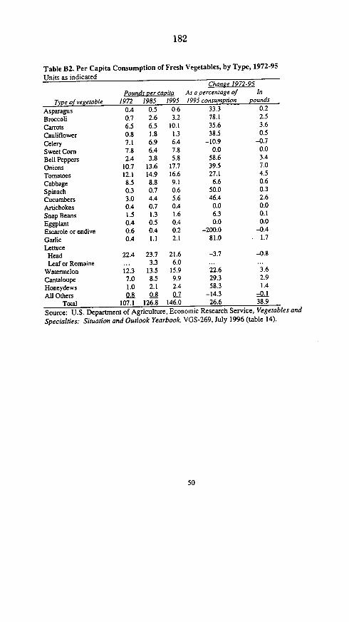
182
Table B2. Per Capita Consumption of Fresh Vegetables, by Type, 1972-95
Units as indicatedChance 1972-95
Pounds Per capita As a percentage of In
Type of vegetable 1972 1985 1995 1995 consumption pounds
Asparagus 0.4 0.5 0.6 33.3 0.2
Broccoli 0.7 2.6 3.2 78.1 2.5
Carrots 6.5 6.5 10.1 35.6 3.6
Cauliflower 0.8 1.8 1.3 38.5 0.5
Celery 7.1 6.9 6.4 -10.9 -0.7
Sweet Corn 7.8 6.4 7.8 0.0 0.0
Bell Peppers 2.4 3.8 5.8 58.6 3.4
Onions 10.7 13.6 17.7 39.5 7.0
Tomatoes 12.1 14.9 16.6 27.1 4.5
Cabbage 8.5 8.8 9.1 6.6 0.6
Spinach 0.3 0.7 0.6 50.0 0.3
Cucumbers 3.0 4.4 5.6 46.4 2.6
Artichokes 0.4 0.7 0.4 0.0 0.0
Snap Beans 1.5 1.3 1.6 6.3 0.1
Eggplant 0.4 0.5 0.4 0.0 0.0
Escarole or endive 0.6 0.4 0.2 -200.0 -0.4
Garlic 0.4 1.1 2.1 81.0 . 1.7
LettuceHead 22.4 23.7 21.6 -3.7 -0.8
Leaf or Romaine ... 3.3 6.0 ... ...
Watermelon 12.3 13.5 15.9 22.6 3.6
Cantaloupe 7.0 8.5 9.9 29.3 2.9
Honeydews 1.0 2.1 2.4 58.3 1.4
All Others 0.8 0.8 0.7 -14.3 -0. 1
Total 107.1 126.8 146.0 26.6 38.9
Source: U.S. Department of Agriculture, Economic Research Service, Vegetables and
Specialties: Situation and Outlook Yearbook, VGS-269, July 1996 (table 14).
50

183
Appendix C. Examples of New Car ReliabilitylDurability Quality Adjustments in the CPI
Since 1992
* Improved corrosion protection -body, electrical system, fuel tank, pump, shocks. brakes and
cables
* Increased warranties
* Body side cladding
* Sealing improvements
* Stainless steel exhaust
* Longer life spark plugs - 100,000 mile life
* Improved steering gears
* Powertrain improvements
* Dextron III transmission fluid - 100,000 mile life
* Water pump front face - 150,000 mile life
* Battery saver
* Increased catalyst load - 100,000 mile life
* Rust resistant fuel injection -100,000 mile life
* Clearcoat paint
* sided galvanized steel body panels
* Serpentine drive belt
51
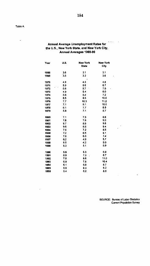
184
Table A.
Annual Average Unemployment Rates forthe U.S., New York State, and New York City,
Annual Averages 1968-96
Year U.S. New York New YorkState City
1968 3.6 3.1 3.11969 3.5 3.3 3.6
1970 4.9 4.5 4.81971 5.9 6.6 6.71972 5.6 6.7 7.01973 4.9 5.4 6.01974 5.6 6.4 7.21975 8.5 9.5 10.61976 7.7 10.3 11.21977 7.1 9.1 10.01978 6.1 7.7 8.91979 5.8 7.1 8.7
1980 7.1 7.5 8.61981 7.6 7.6 9.01982 9.7 8.6 9.61983 9.6 8.6 9.41984 7.5 7.2 8.91985 7.2 6.5 8.11986 7.0 6.3 7.41987 6.2 4.9 5.71988 5.5 4.2 5.01989 5.3 5.1 6.9
1990 5.6 5.3 6.91991 6.8 7.3 8.71992 7.5 8.6 11.01993 6.9 7.8 10.41994 6.1 6.9 8.71995 5.6 6.3 8.21996 5.4 6.2 8.8
SOURCE: Bureau of Labor StabsticCurrent Population Survey

185
Table B.
Annual Average Unemployment Rates forthe 20 Largest Cities, 1990 and 1996
City
New YorkLos AngelesChicagoHoustonPhiladelphiaSan DiegoDallasPhoenixDetroitSan AntonioSan JoseIndianapolisSan FranciscoBaltimoreJacksonvilleColumbusMihaukeeMemphisWashington, DCBoston
1990 1996
6.9 8.86.7 9.38.4 6.76.1 6.46.3 6.94.8 5.46.2 5.24.9 4.014.3 9.17.9 4.94.7 4.23.8 3.73.8 4.78.2 8.15.3 3.83.9 3.45.7 5.15.4 5.36.6 8.55.7 4.5
Population ranking is based on 1992 population.
SOURCE: Bureau of Labor StatisticsLocal Area Unemployment Statistics

186
Table C.
Labor Force Participation Rates, Employment-Population Ratios,and Unemployment Rates by Sex, Age, Race, and Hispanic Origin
for the U.S. and New York City,1996 Annual Averages
Labor Force Employment- UnemploymentPopulation Group Participation Rates Populaion Ratio Rate
U.S. I N.Y.C. U.S. N.Y.C. U.S. | N.Y.C.
Total 66.8 56.7 63.2 51.7 5.4 8.8Men 74.9 66.4 70.9 60.4 5.4 9.0Women 59.3 48.7 56.0 44.5 5.4 8.5Both sexes, 16-19 years 52.3 25.0 43.5 17.8 16.7 29.0
White 67.2 55.7 64.1 51.6 4.7 7.4
Black 64.1 55.4 57.4 48.4 10.5 12.5
Hispanic origin 66.5 52.7 60.6 47.0 8.9 10.8
SOURCE: Bureau of Labor StatisticsCurrent Population Survey

187
Table D.
Unemployment Rates by Occupationfor the U.S. and New York City,
1996 Annual Averages
Occupational Category
Managenal and Professional SpecialtyExecutive, Administrative & ManagenalProfessional
Technical, Sales, & Administrative SupportTechnical and Related SupportSales
Administrative Support (includes clerical)
Service Occupations
Precision Production. Craft. & Repair
Operators, Fabricators, & LaborersMachine Operators, Assemblers, & InspectorsTransportation & Material MovingHandlers, Equipment Cleaners, Helpers, & Laborers
United States New York City
2.4 3.22.3 4.5
2.8 5.65.2 9.54.2 8.9
7.2 9.4
5.5 11.0
7.75.2
11.1
11.36.316.7
NOTE: Occupational detail excludes persons with no previous work experience.Farming and fishing occupations are not shown separately.
SOURCE: Bureau of Labor StatisticsCurrent Population Survey

188
Table E.
Unemployment Rates by Industryfor Nonagricultural Workers
in the U.S. and New York City,1996 Annual Averages
Industry
ConstructionManufacturing
TotalDurable GoodsNondurable Goods
Transportation, Communications and Public UtilitiesTradeFinance, Insurance & Real EstateServices
Government
United States New York City
10.1 17-2
4.8 8.74.5 10.45.2 8.14.1 8.16.4 10.92.7 5.05.4 8.22.8 4.6
NOTE: Industry detail excludes persons with no previous work experience.
SOURCE: Bureau of Labor StatisticsCurrent Population Survey

189
Table F.
Percent of Employed Persons in Occupationsby Demographic Group,
for the U.S. and New York City,1996 Annual Averages
Occupational Category
TotalManagerial and Professional Specialty
Executive, Administrative & ManagerialProfessional
Technical, Sales, & Administrative SupportTechnical and Related SupportSales
Administrative Support (includes clerical)
Service Occupations
Precision Production, Craft, & Repair
Operators, Fabricators, & LaborersMachine Operators, Assemblers, & InspectorsTransportation & Material MovingHandlers. Equipment Cleaners. Helpers, & Laborers
New York City United StatesPercent of total Percent of total
Women Black Hispanic Women Black Hispanicorigin origin
471 27.2 22.7 46.2 10.7 92
43.2 16.3 11.5 438 69 4857.0 20.2 9.7 533 79 43
48.6 24.3 20.0 52.5 9.4 6.341.5 18.0 174 495 79 7070.1 35.0 237 791 125 83
52.0 38.0 32.4 594 17.2 13.7
78 28.8 26.9 90 7.9 110
51.4 20.7 51.4 37.7 15.2 16.421 39.4 24.5 9.5 14.6 10398 284 37.3 193 164 15.2
NOTE Occupational detail excludes persons with no previous work experienceTotal includes farming and fishing, not shown separately.
SOURCE Bureau of Labor StatisticsCurrent Population Survey
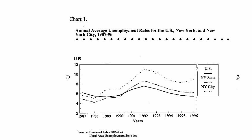
Chart 1.
Annual Average Unemployment Rates for the U.S., New York, and NewYork City, 1987-96
U R12
U.S.
010 - - ~~~~~~~~~~~~~~NY State
8 - ~~~~~~~~~~~~~~NY City
4
Source: Bureau of Labor StatisticsLbcal Area Unemployment Statistics
2 l l l l l l l I1987 1988 1989 1990 1991 1992 1993 1994 1995 1996
Years

ISBN 0-16-055374-1
1 17811 11 1155374519 780160 553745--- --


![BEFORE THE JOINT ECONOMIC COMMITTEE CONGRESS OF THE … · (II) JOINT ECONOMIC COMMITTEE [Created pursuant to Sec. 5(a) of Public Law 304, 79th Congress] HOUSE OF REPRESENTATIVES](https://img.dokumen.tips/doc/110x75/5f3ac3529f8a1c7bbc2a9514/before-the-joint-economic-committee-congress-of-the-ii-joint-economic-committee.jpg)