Embed Size (px)
Citation preview
Iyer - Lecture 16
ECE 313 - Fall 2013
Joint Distribution Functions, Independent Random Variables
ECE 313 Probability with Engineering Applications
Lecture 16 Professor Ravi K. Iyer
Dept. of Electrical and Computer Engineering University of Illinois at Urbana Champaign

Iyer - Lecture 16
ECE 313 - Fall 2013
Announcements
• Midterm next Tuesday, October 22 11:00am – 12:20pm, in class
– All topics covered in Lectures 1 to 15 – Homework 1-6, In-class projects 1-3, and Mini-Projects 1-2
• Be on time, exam starts at 11:00am sharp. • You are allowed to bring only one 8”x11” sheet of notes
• Review Session Today, 5:00pm – 7:00pm, CSL 141
• Additional TA Office hours on Friday, 2:00pm – 5pm, CSL 249.

Iyer - Lecture 16
ECE 313 - Fall 2013
Today’s Topics
• Quick Review on Joint Distribution Functions
– Example
• Independence of Random Variables
• Review of Material for the Midterm Exam

Iyer - Lecture 16
ECE 313 - Fall 2013
Joint Distribution Functions
• We have concerned ourselves with the probability distribution of a single random variable
• Often interested in probability statements concerning two or more random variables
• Define, for any two random variables X and Y, the joint cumulative probability distribution function of X and Y by
• The distribution of X can be obtained from the joint distribution of X and Y as follows:
∞<<∞−≤≤= babYaXPbaF ,},,{),(
),( },{
}{)(FX
∞=∞<≤=
≤=
aFYaXP
aXPa
Iyer - Lecture 16
ECE 313 - Fall 2013
Joint Distribution Functions Cont’d
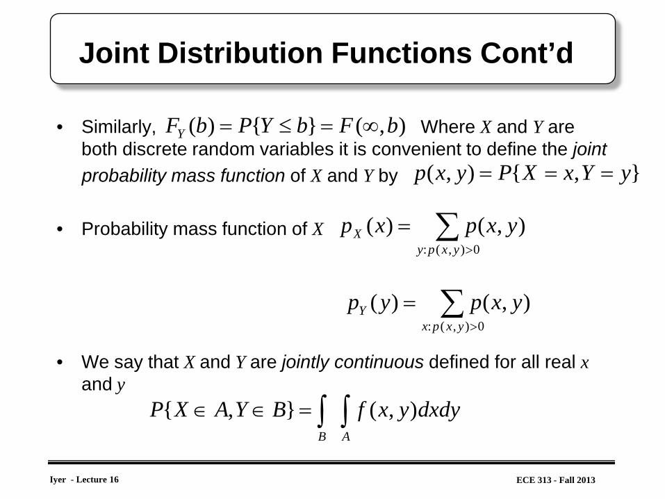
• Similarly, Where X and Y are both discrete random variables it is convenient to define the joint
probability mass function of X and Y by
• Probability mass function of X
• We say that X and Y are jointly continuous defined for all real x and y
),(}{)( bFbYPbFY ∞=≤=
},{),( yYxXPyxp ===
∑>
=0),(:
),()(yxpy
X yxpxp
∑>
=0),(:
),()(yxpx
Y yxpyp
∫∫=∈∈AB
dxdyyxfBYAXP ),(},{

Iyer - Lecture 16
ECE 313 - Fall 2013
Joint Distribution Functions Cont’d
• Called the joint probability density function of X and Y. The probability density of X is thus the probability density function of X
• Similarly the probability density function of Y is because
∫∫∫
=
=
∞−∞∈∈=∈∞
∞−
A X
A
dxxf
dxdyyxf
YAXPAXP
)(
),(
)},(,{}{
∫∞
∞−= dyyxfxf X ),()(
∫∞
∞−= dxyxfyfY ),()(
∫∫ ∞−∞−=≤≤=
badydxyxfbYaXPbaF ),(),(),(
Iyer - Lecture 16
ECE 313 - Fall 2013
Joint Distribution Functions Cont’d
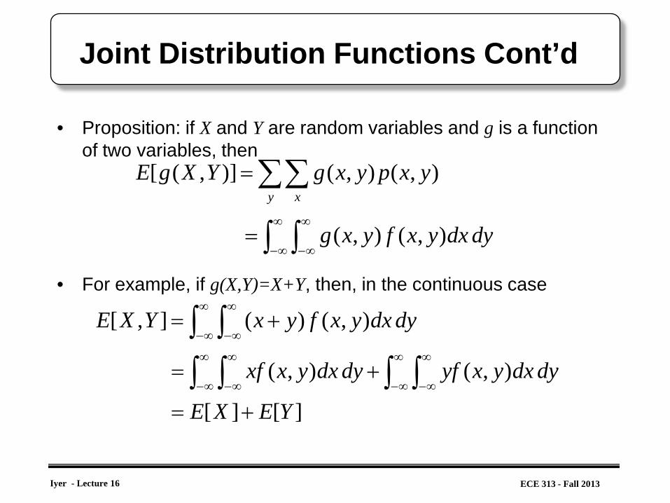
• Proposition: if X and Y are random variables and g is a function of two variables, then
• For example, if g(X,Y)=X+Y, then, in the continuous case
dydxyxfyxg
yxpyxgYXgEy x
),(),(
),(),()],([
∫ ∫
∑∑∞
∞−
∞
∞−=
=
][][
),(),(
),()(],[
YEXE
dydxyxyfdydxyxxf
dydxyxfyxYXE
+=
+=
+=
∫ ∫∫ ∫∫ ∫
∞
∞−
∞
∞−
∞
∞−
∞
∞−
∞
∞−
∞
∞−

Iyer - Lecture 16
ECE 313 - Fall 2013
Joint Distribution Functions Cont’d
• Where the first integral is evaluated by using the foregoing Proposition with g(x,y)=x and the second with g(x,y)=y
• In the discrete case • Joint probability distributions may also be defined for n random
variables. If are n random variables, then for any n constants
nXXX ,...,, 21
][][][ YbEXaEbYaXE +=+
naaa ,...,, 21
][...][][]...[ 22112211 nnnn XEaXEaXEaXaXaXaE +++=++
Iyer - Lecture 16
ECE 313 - Fall 2013
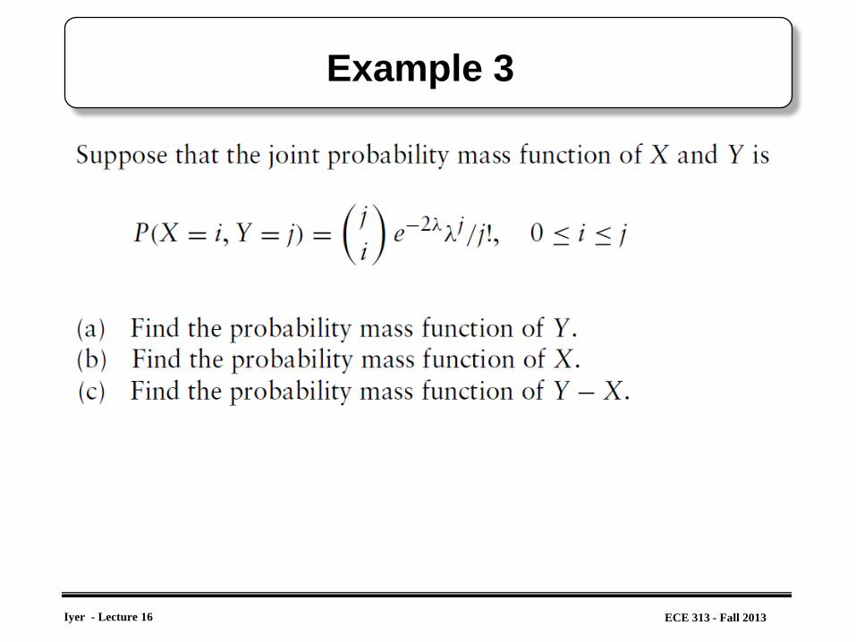
Example 3

Iyer - Lecture 16
ECE 313 - Fall 2013
Example 3 (Cont’d)
a) Marginal PDF of Y:
b) Marginal PDF of X:
Iyer - Lecture 16
ECE 313 - Fall 2013
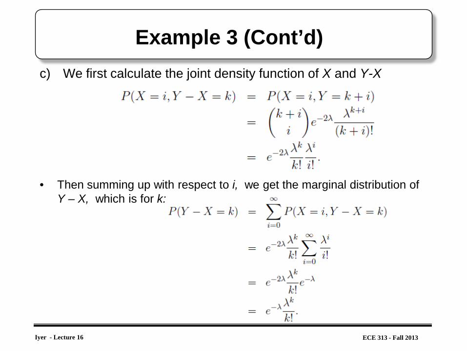
Example 3 (Cont’d) c) We first calculate the joint density function of X and Y-X
• Then summing up with respect to i, we get the marginal distribution of Y – X, which is for k:

Iyer - Lecture 16
ECE 313 - Fall 2013
Independent Random Variables
• We define two random variables X and Y to be independent if:
• Independence of random variables X and Y implies that their joint CDF factors into the product of the marginal CDFs.
• Applies to all types of random variables • In case X and Y are discrete, the preceding definition of
independence is equivalent to • If X and Y are continuous, the preceding definition of
independence is equivalent to the condition assuming that f(x,y) exists.
• The joint distribution of X and Y when one of them is a discrete random variable while the other is a continuous random variable
∞<<−∞∞<<∞−= yxyFxFyxF YX ,),()(),(
)()(),( yPxPyxp YX=
∞<<−∞∞<<∞−= yxyfxfyxf YX ,),()(),(

Iyer - Lecture 16
ECE 313 - Fall 2013
Independent Random Variables Cont’d
• If X is discrete and Y is continuous their independence becomes:
• The definition of joint distribution, joint density, and independence of two random variables can be easily generalized to a set of n random variables,
• Example (Independent R.V.) • Assume that the lifetime X and the brightness Y of a light bulb
are being modeled as continuous random variables. Let the joint pdf be given by
• This is known as the bivariate exponential density. • The marginal density of X is
∞<<∞<<= +− yxeyxf yx 0,0,),( )(21
21 λλλλ
.,...,, 21 nXXX
Iyer - Lecture 16
ECE 313 - Fall 2013
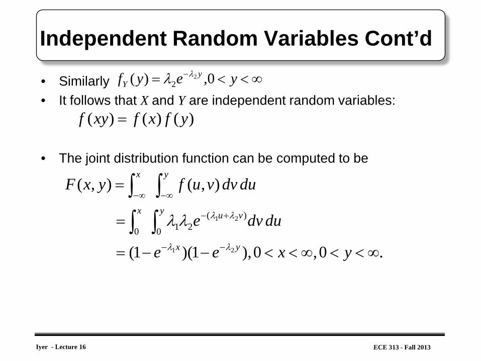
Independent Random Variables Cont’d
• Similarly • It follows that X and Y are independent random variables:
• The joint distribution function can be computed to be
∞<<= − yeyf yY 0,)( 2
2λλ
.0,0),1)(1(
),(),(
21
21
0
)(210
∞<<∞<<−−=
=
=
−−
+−
∞−∞−
∫∫∫∫
yxee
dudve
dudvvufyxF
yx
y vux
yx
λλ
λλλλ
)()()( yfxfxyf =

Iyer - Lecture 16
ECE 313 - Fall 2013
Exam Review
• Basic Concepts: – Random experiment is an experiment the outcome of which is not certain – Sample Space (S) is the totality of the possible outcomes of a random
experiment – Discrete (countable) sample space is a sample space which is either
• finite, i.e., the set of all possible outcomes of the experiment is finite • countably infinite, i.e., the set of all outcomes can be put into a one-
to-one correspondence with the natural numbers – Continuous sample space is a sample space for which all elements
constitute a continuum, such as all the points on a line, all the points in a plane
– An event is a collection of certain sample points, i.e., a subset of the sample space • Universal event is the entire sample space S • The null set ∅ is a null or impossible event
Iyer - Lecture 16
ECE 313 - Fall 2013
Exam Review
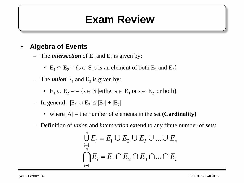
• Algebra of Events – The intersection of E1 and E2 is given by:
• E1 ∩ E2 = {s ∈ S |s is an element of both E1 and E2}
– The union E1 and E2 is given by:
• E1 ∪ E2 = = {s ∈ S |either s ∈ E1 or s ∈ E2 or both}
– In general: |E1 ∪ E2| ≤ |E1| + |E2|
• where |A| = the number of elements in the set (Cardinality)
– Definition of union and intersection extend to any finite number of sets:
Iyer - Lecture 16
ECE 313 - Fall 2013
Exam Review
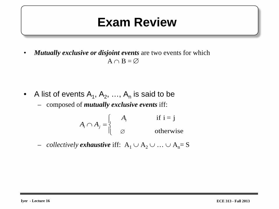
• Mutually exclusive or disjoint events are two events for which A ∩ B = ∅
• A list of events A1, A2, …, An is said to be – composed of mutually exclusive events iff:
– collectively exhaustive iff: A1 ∪ A2 ∪ … ∪ An= S
=∩otherwise
j = i if i
ji
AAA
∅

Iyer - Lecture 16
ECE 313 - Fall 2013
Exam Review
• Probability Axioms – Let S be a sample space of a random experiment and P(A) be the
probability of the event A – The probability function P(.) must satisfy the three following axioms: – (A1) For any event A, P(A) ≥ 0 (probabilities are nonnegative real numbers) – (A2) P(S) = 1 (probability of a certain event, an event that must happen is equal 1) – (A3) P(A ∪ B) = P(A) + P(B), whenever A and B are mutually exclusive
events, i.e., A ∩ B = ∅ (probability function must be additive) – (A3’) For any countable sequence of events A1, A2, …, An …, that are
mutually exclusive (that is Aj ∩ Ak = ∅ whenever j ≠ k)

Iyer - Lecture 16
ECE 313 - Fall 2013
Exam Review
• (Ra) For any event A, P( ) = 1 - P(A) • (Rb) If ∅ is the impossible event, then P(∅) = 0 • (Rc) If A and B are any events, not necessarily mutually
exclusive, then P (A ∪ B) = P(A) + P(B) - P (A ∩ B)
• (Rd)(generalization of Rc) If A1, A2, …, An are any events, then
where the successive sums are over all possible events, pairs of events, triples of events, and so on.
(Can prove this relation by induction (see class web site))

Iyer - Lecture 16
ECE 313 - Fall 2013
Exam Review
• Combinatorial Problems – Permutations with replacement:
• Ordered samples of size k, with replacement P(n, k) – Permutations without replacement
• Ordered Samples of size k, without replacement
– Combinations • Unordered sample of size k, without replacement
• Binomial Theorem
k)!(nn!1)k1)....(nn(n−
=+−− k = 1, 2, …, n
nk
=
n!k!(n − k)!
Iyer - Lecture 16
ECE 313 - Fall 2013
Exam Review
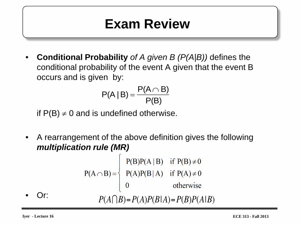
• Conditional Probability of A given B (P(A|B)) defines the conditional probability of the event A given that the event B occurs and is given by:
if P(B) ≠ 0 and is undefined otherwise.
• A rearrangement of the above definition gives the following multiplication rule (MR)
• Or:
P(A | B) =
P(A ∩ B)P(B)

Iyer - Lecture 16
ECE 313 - Fall 2013
Exam Review • Theorem of Total Probability • Any event A can be partitioned into two disjoint subsets:
• Then:
• In general:
• Bayes Formula:
)()( BABAA ∩∪∩=
)()|()()|(
)()()(
BPBAPBPBAP
BAPBAPAP
+=
∩∪∩=
∑ ==
n
i ii BPBAPAP1
)()|()(
∑=
∩=
iii
jjjj BPBAP
BPBAPAP
ABPABP
)()|()()|(
)()(
)|(
Iyer - Lecture 16
ECE 313 - Fall 2013
Exam Review
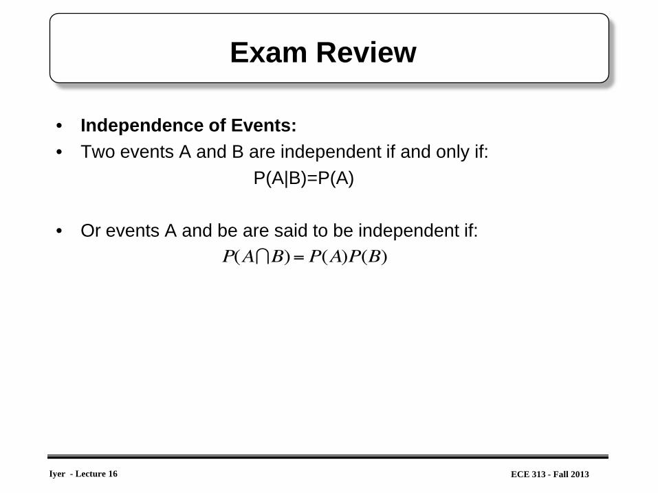
• Independence of Events: • Two events A and B are independent if and only if: P(A|B)=P(A) • Or events A and be are said to be independent if:
Iyer - Lecture 16
ECE 313 - Fall 2013
Exam Review
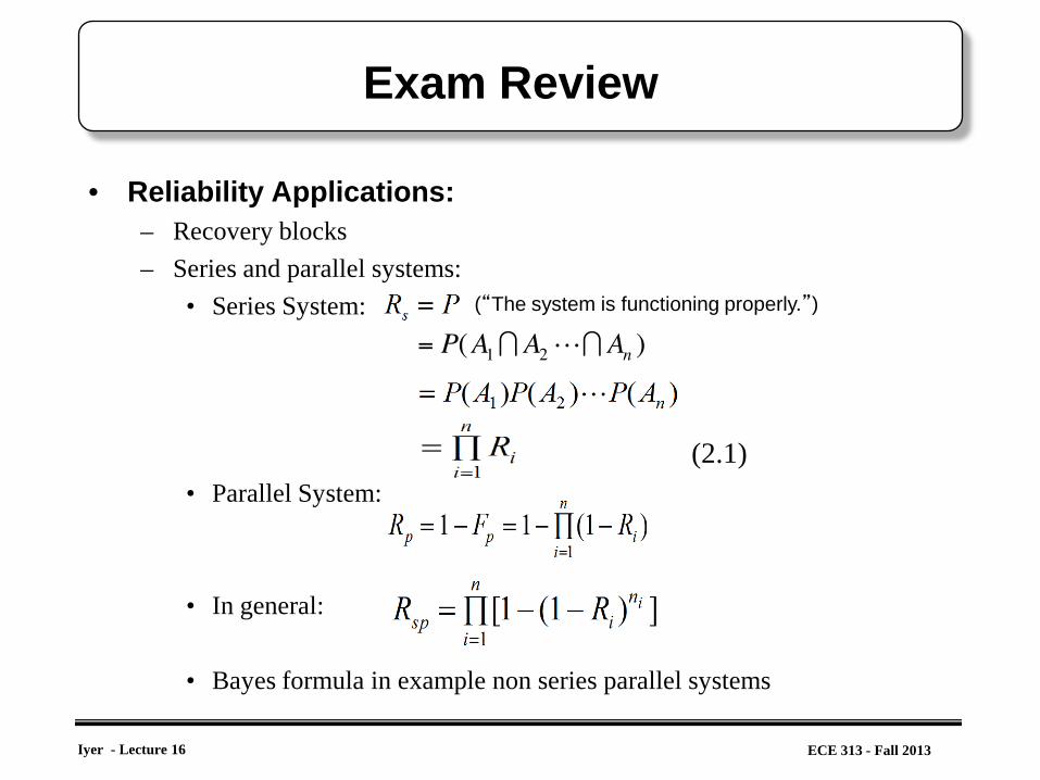
• Reliability Applications: – Recovery blocks – Series and parallel systems:
• Series System:
• Parallel System:
• In general:
• Bayes formula in example non series parallel systems
(2.1)
(“The system is functioning properly.”)
Iyer - Lecture 16
ECE 313 - Fall 2013
Exam Review
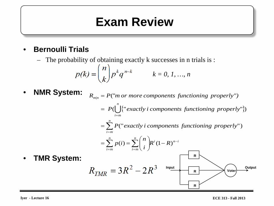
• Bernoulli Trials – The probability of obtaining exactly k successes in n trials is :
• NMR System:
• TMR System:
k = 0, 1, …, n
{ }
∑∑
∑
=
−
=
=
=
−
==
=
=
=
n
mi
inin
mi
n
mi
n
mi
nm
RRin
ip
properly gfunctionin components iexactly P
properly gfunctionin components iexactly P
") properly gfunctionin components more or m"PR
)1()(
)"("
)""(
(|
R
R
R
Voter Output Input
Iyer - Lecture 16
ECE 313 - Fall 2013
Exam Review
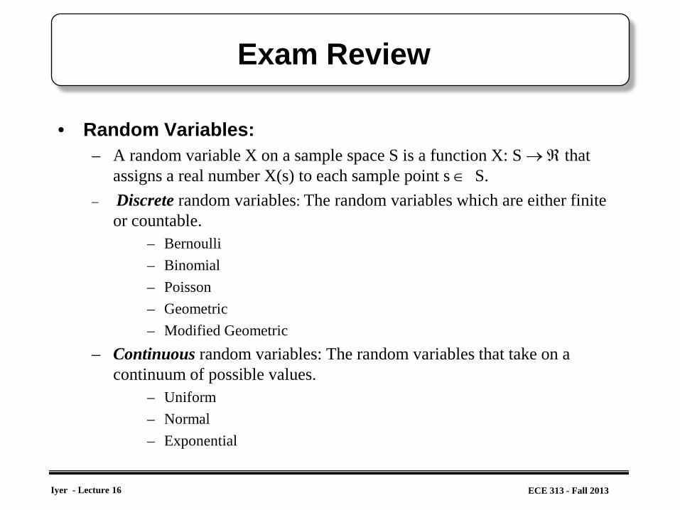
• Random Variables: – A random variable X on a sample space S is a function X: S → ℜ that
assigns a real number X(s) to each sample point s ∈ S. – Discrete random variables: The random variables which are either finite
or countable. – Bernoulli – Binomial – Poisson – Geometric – Modified Geometric
– Continuous random variables: The random variables that take on a continuum of possible values.
– Uniform – Normal – Exponential
Iyer - Lecture 16
ECE 313 - Fall 2013
Exam Review
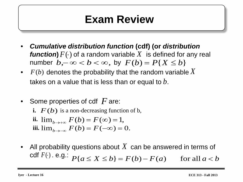
• Cumulative distribution function (cdf) (or distribution function) of a random variable is defined for any real number by
• denotes the probability that the random variable takes on a value that is less than or equal to .
• Some properties of cdf are:
i. is a non-decreasing function of b, ii. iii.
• All probability questions about can be answered in terms of
cdf . e.g.:
)(⋅F X,, ∞<<∞− bb }{)( bXPbF ≤=
)(bF Xb
F)(bF
,1)()(lim =∞=+∞→ FbFb.0)()(lim =−∞=−∞→ FbFb
)(⋅F baaFbFbXaP <−=≤≤ allfor )()(}{
X
Iyer - Lecture 16
ECE 313 - Fall 2013
Exam Review
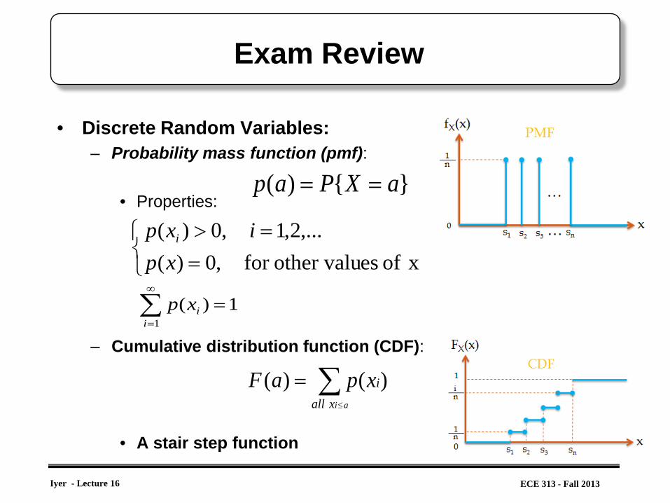
• Discrete Random Variables: – Probability mass function (pmf):
• Properties:
– Cumulative distribution function (CDF):
• A stair step function
}{)( aXPap ==
==>
xof esother valufor ,0)(,...2,1,0)(
xpixp i
1)(1
=∑∞
=iixp
∑≤
=aixall
ixpaF )()(

Iyer - Lecture 16
ECE 313 - Fall 2013
Exam Review
• Continuous Random Variables: – Probability distribution function (pdf):
• Properties:
• All probability statements about X can be answered by f(x):
– Cumulative distribution function (CDF):
• Properties:
• A continuous function
∫∞
∞−=∞−∞∈= dxxfXP )()},({1
∫=≤≤b
adxxfbXaP )(}{
∫ ===a
adxxfaXP 0)(}{
)()( afaFdad
=
∫∞−
∞<<∞−=≤=x
xx xdttfxXPxF , )()()(

Iyer - Lecture 16
ECE 313 - Fall 2013
Exam Review
• Summary of important distributions:
Iyer - Lecture 16
ECE 313 - Fall 2013
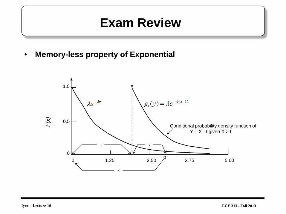
Exam Review
• Memory-less property of Exponential F(
x)
0
1.0
0.5
1.25 2.50 3.75 5.00 0
t y
x
Conditional probability density function of Y = X - t given X > t
Iyer - Lecture 16
ECE 313 - Fall 2013
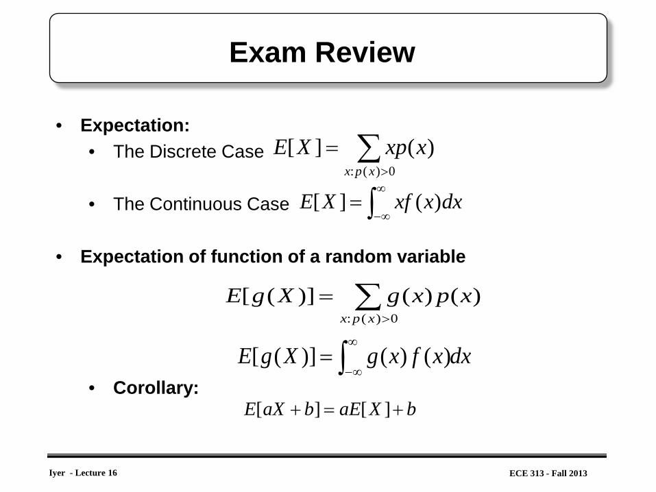
• Expectation: • The Discrete Case
• The Continuous Case
• Expectation of function of a random variable
• Corollary:
Exam Review
∑>
=0)(:
)(][xpx
xxpXE
∫∞
∞−= dxxxfXE )(][
∑>
=0)(:
)()()]([xpx
xpxgXgE
dxxfxgXgE ∫∞
∞−= )()()]([
bXaEbaXE +=+ ][][
Iyer - Lecture 16
ECE 313 - Fall 2013
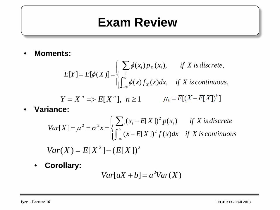
Exam Review
• Moments:
• Variance: • Corollary:
−
−===
∫∑∞
∞−continuousisXifdxxfXEx
discreteisXifxpXExxXVar i ii
)(])[(
)(])[(][ 2
2
22 σµ
==∫
∑∞
∞−,,)()(
,),()()]([][
continuousisXifdxxfx
discreteisXifxpxXEYE
X
iiXi
φ
φφ
1],[ ≥=>= nXEXY nn
22 ])[(][)( XEXEXVar −=
)(][ 2 XVarabaXVar =+
Iyer - Lecture 16
ECE 313 - Fall 2013
Exam Review
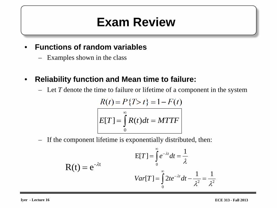
• Functions of random variables – Examples shown in the class
• Reliability function and Mean time to failure:
– Let T denote the time to failure or lifetime of a component in the system
– If the component lifetime is exponentially distributed, then:
∫∞
==0
)(][ MTTFdttRTE
t-eR(t) λ=22
0
0
112][
1][E
λλ
λ
λ
λ
=−=
==
∫
∫∞
−
∞−
dtteTVar
dteT
t
t
Iyer - Lecture 16
ECE 313 - Fall 2013
Exam Review
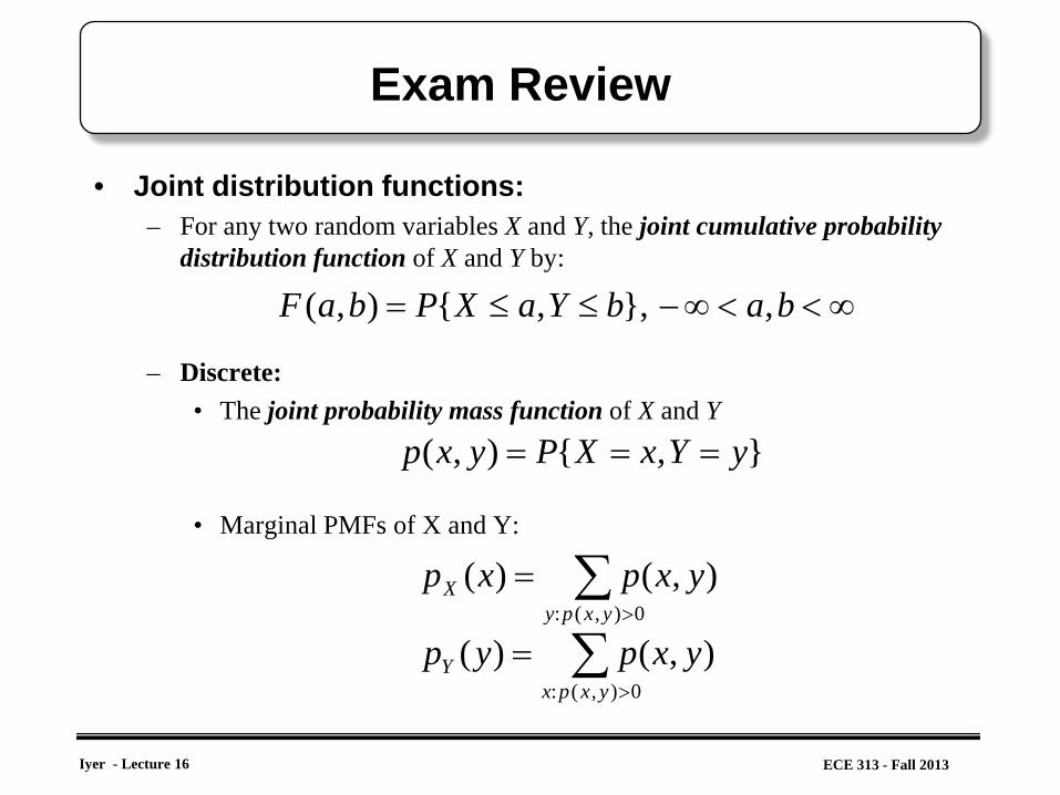
• Joint distribution functions: – For any two random variables X and Y, the joint cumulative probability
distribution function of X and Y by:
– Discrete: • The joint probability mass function of X and Y
• Marginal PMFs of X and Y:
∞<<∞−≤≤= babYaXPbaF ,},,{),(
},{),( yYxXPyxp ===
∑>
=0),(:
),()(yxpy
X yxpxp
∑>
=0),(:
),()(yxpx
Y yxpyp
Iyer - Lecture 16
ECE 313 - Fall 2013
Exam Review
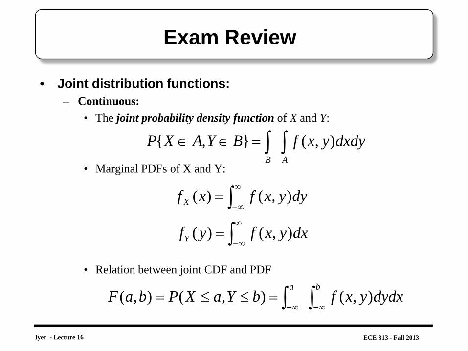
• Joint distribution functions: – Continuous:
• The joint probability density function of X and Y:
• Marginal PDFs of X and Y:
• Relation between joint CDF and PDF
∫∫=∈∈AB
dxdyyxfBYAXP ),(},{
∫∞
∞−= dyyxfxf X ),()(
∫∞
∞−= dxyxfyfY ),()(
∫∫ ∞−∞−=≤≤=
badydxyxfbYaXPbaF ),(),(),(

Iyer - Lecture 16
ECE 313 - Fall 2013
Exam Review
• Function of two joint random variables
• For example, if g(X,Y)=X+Y, then, in the continuous case
dydxyxfyxg
yxpyxgYXgEy x
),(),(
),(),()],([
∫ ∫
∑∑∞
∞−
∞
∞−=
=

Iyer - Lecture 16
ECE 313 - Fall 2013
Exam Review
• Independent Random Variables: Two random variables X and Y are said to be independent if:
• If X and Y are continuous:
• If X is discrete and Y is continuous:
∞<<−∞∞<<∞−= yxyFxFyxF YX ,),()(),(
∞<<−∞∞<<∞−= yxyfxfyxf YX ,),()(),(