Johns Hopkins APL

TECH N I CAL DIG EST July-September 1980, Vol. 1, No. 3

The Magsat issue

Editorial Board

Walter G. Berl, Chairman Frederick S. Billig Billy D. Dobbins Morton H. Friedman Robert W. Hart Samuel Koslov Vincent L. Pisacane Gary L. Smith Robert J. Thompson, Jr .

Ex Officio Edward L. Cochran M. B. Gilbert Vernon M. Root

Editorial Staff

M. B. Gilbert, Managing Editor Jerome W. Howe, Associate Editor Stephen G. Smith, Art Director Daryl L. George, Staff Artist David W. Sussman, Staff Photographer

The Johns Hopkins APL Technical Di­gest (ISSN 0001-2211), established in 1961 as the APL Technical Digest, is published quarterly under the auspices of The Johns Hopkins University Ap­plied Physics Laboratory (JHU/ APL), Johns Hopkins Road, Laurel, Md . 208lO. The objective of the publication is to provide a summary of unclassified individual programs under way at JHU/ APL. Requests for free individual copies, free subscriptions, or permission to reprint the text should be submitted to the Managing Editor.

Postmaster: Send address changes to that address. Second-class postage paid at Laurel, Md.

© 1980 by The Johns Hopkins Univer­sity Applied Physics Laboratory.

fohns Hopkins APL

TECHNICAL DIGEST July-September 1980, Volume 1, Number 3

The Magsa[ issue

TECHNICAL ARTICLES

162 The Geomagnetic Field and Its Measurement: Introduction and Magnetic Field Satellite (Magsat) Glossary

171 Overview of the Magsat Program

175 Magsat Performance Highlights

179 The Magsat Power System

183 The Magsat Telecommunications System

188 The Magsat Attitude Control System

194 The Magsat Attitude Determination System

201 The Magsat Magnetometer Boom System

205 The Magsat Scalar Magnetometer

210 The Magsat Precision Vector Magnetometer

214 Magsat Scientific Investigations

228 Studies of Auroral Field-Aligned Currents with Magsat

SPECIAL TOPIC

233 China - As Viewed by an Aerospace Engineer

DEP ARTMENTS

240 Publications, Presentations, APL Colloquia, The Authors

Front Cover:

T. A . Potemra, F. F. Mobley, L. D. Eckard

G. W. Ousley

F. F. Mobley

W. E. Allen

A . L. Lew, B. C. Moore, J . R . Dozsa, R . K. Burek

K. J . Heffernan, G. H. Foun/ain, B. E. Tossman, F. F. Mobley

G. H. Foun/ain, F. W. Schenkel, T. B. Coughlin, C. A. Wingate

J. F. Smola,

W. H. Farthing

M. H. Acuna

R . A . Langel

T. A. POlemra

F. S. Billig

Conceptual painting by S. G. Smith of the Digest staff. The earth, showing the magnetic anomalies mea­sured by Magsat and earlier satellite vehicles, is silhouetted against the frontispiece of Gilbert's seminal trea­tise on geomagnetism (De Magnete, second edition, 1628). A line drawing of Magsat IS in the foreground.

THOMAS A. POTEMRA, FREDERICK F. MOBLEY, and LEWIS D. ECKARD

THE GEOMAGNETIC FIELD AND ITS MEASUREMENT: INTRODUCTION AND MAGNETIC FIELD SATELLITE (MAGSAT) GLOSSARY

The earth's magnetic field, its measurement by conventional methods, and the specific objec­tives and functions of the Magsat system to obtain precise absolute and directional values of the earth's magnetic field on a global scale are briefly described.

EARLY HISTORY The directional property of the earth's magnetic

field has been appreciated by the Chinese for more than 4500 years. Records indicate I that in 2634 B.C. the Chinese emperor Hoang-Ti was at war with a local prince named Tchi-Yeou and that they fought a great battle in the plain of Tcho-Iuo. Tchi-Yeou raised a dense fog that produced disorder in the imperial army - a forerunner of the modern smokescreen . As a countermeasure, Hoang-Ti con­structed a chariot on which stood the small figure of a man with his arm outstretched. This figure, apparently free to revolve on its vertical axis , always pointed to the south, allowing the emperor to locate the direction of his enemy's retreat. Tchi­Yeou was captured and put to death.

The first systematic and scientific study of the earth's magnetic field was conducted by William Gilbert, physician (later promoted to electrician) to Queen Elizabeth, who published in 1600 his procla­mation "Magnus magnes ipse est globus ter­restrius" (the earth globe itself is a great magnet) in his De Magnete. 2 This treatise was published nearly a century before Newton's Philosophiae Naturalis Principia Mathematica (1687), and it has been suggested that Gilbert invented the whole pro­cess of modern science rather than merely having discovered the basic laws of magnetism and of static electricity.3 Gilbert' s efforts may have been inspired by the need for Her Majesty's Navy to im­prove (if not understand) the principal means of navigation - the magnetic compass. This fact is evident from the frontispiece of the second Latin edition of De Magnete, (Fig. 1) published in 1628.

An understanding of the earth's magnetic field and its variations is still of great importance to navigators. (More recently the U.S . Navy has "in­spired" APL to develop and improve a more ad­vanced satellite system for navigation.) The geo-

162

PKYSIOLOGIA NOVA

D£MAGNETL MAGNETICI SQVE CORPO' RIBVS ET MAGNO MAG~ETE tc\1ure Sox Iibris. comprehcn[us

Guiliclmo Gilbcrl~ colcef1rcnG , Modico Londincnri . .

ill '1U1b"; (a ,,!U{( ad ~an( malrrinm fpcc/an!.",!,, · mrs dar:.qumm!tsat (Xff'nmmf!s (~ac1!fslm('

a':f'lu1!ftlmr~ ~r4dal171lr d 'Y!t (Il~fu r . Omnia nuncdihgcntcr rccognlta lk ernen,

dalius quam ank '" lucom <plta,auda 8<: flgu , n! illuJlrat~ opera&: AudiO

wolfoangi>to'~man6 / 1 . U . D . .:J & Mathernali. .

Ad calcrm librilldjunciu; fS llndrxCapl ,. fum Rfrnm rl Vrrborum IOCllflrl ift lmus

ExCVSVS SEDIN I Typis G6tzianis Sumpfibus

../fufhorlS dnnoM.DC.XXVlII .

Fig. 1-The engraved title page from the second Latin edition of Gilbert 's De Magnete. It shows lodestones, compasses, and a terrella (a small spherical magnet sim­ulating the earth, in the upper left corner). In a vignette at the bottom is a ship sailing away from a floating bowl compass with a terrella at the center. The first edition of De Magnete was published in 1600, and copies have become extremely rare.

magnetic field also plays an important practical role in searching for possible resources beneath the earth's crust and in stabilizing artificial satellites. Major disturbances to the geomagnetic field -called "magnetic storms" - induce large, un-

Johns Hopkins APL Technical Diges(

__________________________________________________ TECHNICALARTICLES

wanted effects in long-distance telephone circuits and sometimes cause widespread power blackouts. The geomagnetic field and its interaction with the continuous flow of ionized gas (plasma) from the sun (the solar wind) provide the basic framework for the complicated space environment of the earth, including the Van Allen radiation belts and auroral zones. The distorted configuration of its geomagnetic field is called the "magnetosphere." Many APL-built spacecraft have made major con­tributions to an understanding of the geomagnetic field and associated magnetospheric phenomena during the past 15 years. Magsat is the latest one to do so.

GEOMAGNETIC FIELD DESCRIPTION The geomagnetic field can be thought of as being

produced by a huge bar magnet imbedded in the earth, with the axis of the magnet tilted away slightly from the earth's rotational axis. The poles of this magnet are located near Thule, Greenland, and Vostok, Antarctica (a U.S.S.R. research sta­tion). To a good approximation, the geomagnetic field can be represented by a simple dipole, but there is a significant contribution from nondipole components and from a system of complicated cur­rents that flow in the magnetospheric regions surrounding the earth. The most accurate represen­tation of the geomagnetic field is provided by a series of spherical harmonic functions. 4 The coef­ficients of such a series representation are evaluated from an international set of spacecraft and surface observations of the geomagnetic field and are pub­lished for a variety of practical uses in navigation and resource surveys. A principal goal of Magsat is to provide the most accurate evaluation of the geo­magnetic field model in this manner (see the article by Langel in this issue).

MAGNETIC UNITS AND TERMINOLOGY A wide variety of units and symbols are currently

in use in the many scientific and engineering fields involved with magnetism. The following definitions are offered in hope of clarifying some of these for a better understanding of the following discussions.

Classic experiments have shown that the force acting on a charged particle moving in a magnetic field is proportional to the magnitude of the charge. A vector quantity known as the "magni­tude induction" is usually denoted by ii which characterizes the magnetic field in a manner similar

Volume I, Number 3,1980

to that done for electric fields by E, for example. This unit of induction, ii, is 1 weber per square meter (1 Wb/m2); it is the magnetic induction of a field in which 1 coulomb of charge, moving with a component of velocity of 1 m/s perpendicular to the field, is acted on by a force of I newton. In SI units, 1 Wb/m 2 = 1 tesla.

In studies of planetary fields, where very small fields are involved, the nanotesla (nT), formerly the "gamma" ('Y), is used where 1 nT = 10.9

tesla = 10-9 Wb/m2 = 1 'Y. (The cgs unit of magnetic intensity is the gauss, where 1 tesla = 104 gauss.) The intensity of the surface geomagnetic field varies from about 30,000 nT at the equator to more than 50,000 nT at high latitudes near the magnetic poles.

SECULAR VARIATION It has been known for over 400 years that the

main geomagnetic field is not steady but experi­ences global secular variations. In fact, from a study of the paleomagnetic properties of igneous rocks, it has been determined that the geomagnetic field has reversed polarity several times over the past 4.5 million years (Fig. 2).5

The behavior of the geomagnetic field over a shorter time scale is shown in Fig. 3. That figure shows the positions of the virtual geomagnetic pole since 1000 A.D. based on the assumption that the geomagnetic field is a centered dipole. 6

The following five features of the secular varia­tion have been determined: 7

1. A decrease in the moment of the dipole field by 0.05070 per year, indicating that the present geomagnetic field may reverse polarity 2000 years from now. Preliminary analysis of Mag­sat data has revealed that this variation may be more rapid than was suspected from previ­ous observations, and that the field may re­verse polarity in only 1400 years;

2. A westward precessional rotation of the di­pole of 0.05 0 of longitude per year;

3. A rotation of the dipole toward the geograph­ic axis of 0.020 of latitude per year;

4 . A westward drift of the nondipole field of 0.20 of longitude per year;

5. Growth and decay of features of the nondi­pole field with average changes of about 10 nT per year.

Although these secular variations necessitate con­tinual corrections to magnetic compasses they pro-

163

Epoch Brunhes Matuyama

II

Gauss

I I 2.13 2.43 2.80

~ Normal field

~ Reversed field

Gilbert

0.93 0.87

1.68 1.85 2.11 2.90 2.94 3.06

Fig. 2-The polarity of the geomagnetic field for the past 4.5 million years deduced from measurements on ig­neous rocks dated by the potassium- argon method and from measurements on cores from ocean sediments (from Ref. 5).

0.350

0.330

0.114

.108

0.02

0.69

Millions of years before present

vide some clues to the internal source of the geo­magnetic field.

GEOMAGNETIC FIELD SOURCES If the average westward drift of the dipole field

in item 2 above is representative of the rate of mo­tion of the field, then the corresponding surface

Fig. 3-The virtual geomagnetic pole positions since 1000 A.D ., which correspond to the secular variations at London if one ascribes the geomagnetic field entirely to a centered dipole. The London variations were deduced from magnetic field orientations of samples obtained from archeological kilns, ovens, and hearths in the southern half of Britain (from Ref. 6). The present virtual pole is located near Thule, Greenland.

164

3.32

3.70

3.92

4.05

4.25

4.38

4.50

velocity is about 20 km per year. This is a million times faster than the large-scale motions of the solid part of the earth deduced from geological ob­servations and considerations. Seismological evi­dence reveals a fluid core for the earth that can easily experience large-scale motions, and it is pre­sumed that the geomagnetic secular variation -and indeed the main field itself - is related to this fluid core. Furthermore, geochemical and density considerations are consistent with a core composed mainly of iron - a good electric and magnetic con­ductor. Therefore, the study of the earth' s internal magnetic field draws in another discipline - mag­netohydrodynamics, which involves moving fluid conductors and magnetic fields.

Modern theories of the geomagnetic field are based on the original suggestion of Larmor that the appropriate internal motion of a conducting fluid could cause it to act as a self-exciting dynamo. S To visualize this, assume the moving core to be an in­finitely good conductor. Any primordial magnetic field lines, outside the core, for example, will be dragged around by the currents within the core as if they were "frozen" into the core. If the core rotates nonuniformly with depth, the field lines will become twisted around the axis of rotation in a way that opposes the initial field. The twisting ac­tion packs the magnetic field lines more closely, causing the field intensity to grow. This growth can neutralize the original field and produce an even larger reversal field. The concept of magnetic field amplification by the differential rotation of con­ductors has been used by astrophysicists to explain the magnetic fields of stars (including the sun), Jupiter, and Saturn. Many theories exist, but the precise generation mechanisms for the internal geomagnetic field are still unknown. 8

MAGNETOSPHERIC CURRENTS When viewed from outer space, the earth's

magnetic field does not resemble a simple dipole

Johns Hopkins APL Technical Diges{

but is severely distorted into a comet-shaped configuration by the continuous flow of plasma (the solar wind) from the sun (depicted in Fig. 4). This distortion demands the existence of a com­plicated set of currents flowing within the distorted magnetic field configuration called the "magneto­sphere." For example, the compression of the geo­magnetic field by the solar wind plasma on the day side of the earth must give rise to a large-scale current flowing across the geomagnetic field lines, called the Chapman-Ferraro or magneto pause cur­rent (see Fig. 4).

The magnetospheric system includes large-scale currents that flow in the "tail"; "Birkeland" cur­rents that flow along geomagnetic field lines (see the article by Potemra in this issue) into and away from the two auroral regions; the ring current that flows at high altitudes around the equator of the earth; and a complex system of currents that flow completely within the layers of the ionosphere, the earth's ionized atmosphere. The intensities of these various currents reach millions of amperes and are closely related to solar activity. They produce mag­netic fields that vary with time scales ranging from a few seconds (micro pulsations) to 11 years (corre­sponding to the solar cycle).

Widespread magnetic disturbances sometimes ob­served over the entire surface of the earth are known as magnetic storms. These storms are asso­ciated with major solar eruptions that emit X rays, ultraviolet and extreme ultraviolet radiations, and particles with energies from I keV to sometimes over 100 MeV. The solar plasma accompanying so­lar eruptions causes a magnetic storm when it col­lides with the earth's magnetosphere. Minor mag-

Solar wind

Fig. 4-The configuration of the earth's dipole magnetic field distorted into the comet·like shape called the mag· netosphere. The various current systems that flow in this complicated plasma laboratory are labeled. The interplan· etary magnetic field is the magnetic field of the sun, which has a modulating effect on the processes that oc­cur within the magnetosphere.

Volume 1, Number 3,1980

netic storms can occur every few weeks during the peak of the II-year solar cycle (the peak of the present cycle is thought to have occurred in 1980), whereas "super" magnetic storms that so severely distort the geomagnetic field as to move the entire auroral zone to lower latitudes are a much rarer event (the last super storm occurred on August 2, 1972, when an aurora was observed in Kentucky). Besides the evaluation of models for the internal geomagnetic field, Magsat, launched in October 1979, provided the most sensitive measurements yet of the magnetospheric current system.

MAGNETIC FIELD MEASUREMENTS The technique of using airplanes for magnetic

field surveys for geological prospecting became well established in the 1950's. Airplanes make their sur­veys at altitudes of 1 to 5 km, whereas satellites or­bit the earth at 200 km or higher. Thus it was somewhat of a surprise when scient ists discovered from the data of the Orbiting Geophysical Obser­vatory satellites in 1972 that useful information about the structure of the earth's crust could be derived from satellite data - information that would be very difficult to detect in airplane survey data. Ideas for a satellite devoted to this objective were discussed for a number of years, finally lead­ing to the Magsat program, which had the addi­tional objective of measuring the "main" field for making new magnetic charts.

MAGSATSPACECRAFT Preliminary discussions among APL, NASA, and

the U.S. Geological Survey (USGS), commencing in the mid-1970's, culminated in conceptual studies of a spacecraft dedicated to the task of completing a global survey of the earth's geomagnetic field. NASA and the USGS subsequently entered into an agreement to conduct such a program on a cooper­ative basis. The Goddard Space Flight Center (GSFC) was selected by NASA as the lead labora­tory for this endeavor. Numerous trade-off design studies were undertaken, with emphasis on flying an adaptation of an available spacecraft design, launched from an early Space Shuttle, as against flying a small spacecraft on a NASA/DoD Scout launch vehicle. However, in view of the uncertain­ties surrounding the availability of the Shuttle, and in light of the desire of USGS to incorporate satel­lite magnetic field data into their 1980 map up­dates, the decision was made by early 1977 to pro­ceed with a Scout-launched spacecraft.

In April 1977, after a successful preliminary de­sign review, APL was funded to proceed with the Magsat design and development effort with the goal of launching the spacecraft by September 21, 1979, at a projected cost of about ten million dollars.

The Small Astronomical Satellite (SAS-3) had been designed and built by APL and launched in

165

1975. Many of the features of SAS-3 seemed ide­ally suited to the magnetic field satellite mission. It was a small spacecraft capable of being launched by the inexpensive Scout rocket, it had the world's most precise tracking system (i.e., positi on determi­nation) in it s Doppler tracking system (a deri va tive of the APL Transit system), it had two star trackers that could provide attitude determination to 10 arc-s (I arc-s = 0.00028) accuracy, and it s attitude control sys tem used an infrared earth­horizon scanner/ momentum wheel assembly that was ideally suited for Magsat. A critical problem, which was quickly id enti fied , was the excessive weight of Magsat. Tape recorders with a large r capacity for data sto rage were needed, a nd new S­band transmitters were required for the high data rate during tape recorder playback. Com promi ses in the solar cell array were necessary to keep the weight down to 182 kg, the maximum that the Scout rocket could launch into a 350 by 500 km or­bit.

MAGSAT ORBIT A n orbit was needed that would give full earth

coverage and as little shadowing by the earth as possible . A polar orbit would be ideal for earth coverage, but because the orbit plane would remain fixed in space, the motion of the earth about the sun would cause shadowing of the satellite within 30 to 60 days after launch. Also, it would be diffi­cult to find star camera orientations that would not present problems with direct sunlight. However, for an orbit inclination of 97", the orbit plane precesses at the rate of 10 / day, just the right amount to make the orbit plane follow the sun. (This precess ion is due to the bulge in the earth's gravity field at the equator.) This sun-synchronous orbi t (Fig. 5) gives nearly 100070 earth coverage and many months of full sunlit orbits. The star cameras

166

could be placed on the dark side of the satellite to avoid direct sunlight.

Even in this case, as the sun approaches the highest latitudes of + 23 0 on June 21, the orbit would be shadowed in the south polar region. Shadowing was expected to begin in April so a launch date of September 1979 was chosen, which would allow six months of fully sunlit orbits. Launch actually occurred at the end of October 1979, so 5 Y2 months of fully sunlit orbits were ob­tained.

THE SPACECRAFT Magsat was intended to measure the vector com­

ponents of the earth's field to an accuracy of 0.01 070; thi s meant that the orientation of the vec­tor sensors must be known to 15 arc-s accuracy. The star cameras were good to an accuracy of 10 arc-s, but they had 2 kg of essential magnetic shielding that would di stort the magnetic field . An extendable boom was needed to put the vector sen­sors 6 meters away from the magnetic disturbance caused by the star cameras. But it was not possible for the boom to be mechanically stable to 5 arc-so A system was needed to measure the orientation of the vector sensors relative to the star cameras. This system, the Attitude Transfer System (ATS), used an opt ical technique involving mirrors attached to the vector sensor to make the necessary measure­ment (see the article by Fountain el 01. in thi s issue).

The elements of the A TS and the two star cameras had to be tied together mechanically in some permanent and extremely stable fashion. The structure to achieve this was the optical bench, a built-up assembly of graphite fiber and epoxy resin that provided a near-zero coefficient of thermal ex­pansion. The bench was attached to the satellite at five point s, two of which were released by pyro­technic devices after the sa tellite was in orbit. The

Fig. 5-The precession of the Magsat orbit plane with time. The Magsat orbit plane makes an angle of 9r with the earth's equatorial plane. At this inclination (and at the altitude of Magsat), the equa­torial bulge of the earth causes the orbit plane to roo tate above the polar axis at 1 '/day, just the right amount to turn the orbit plane toward the sun as the earth proceeds in its orbit about the sun. Un· fortunately , the 23' tilt of the earth polar axis adds to the r tilt of the orbit plane in June, causing shadowing of the southern portion of the orbit by the earth. This shadowing began in mid-April for Magsat.

Johns Hopkins APL Technical Digest

three remaining support points did not apply stress to the bench. Heaters and temperature sensors at eight places stabilized the bench temperature at 25°C.

At the end of the 6 meter extendable boom were the vector magnetometer sensor and a scalar mag­netometer sensor (see the articles by Acuna and Farthing). The vector sensor consisted of three small toroidal cores of highly permeable magnetic material with platinum wire windings used to sense the components of the field. They were mounted on a very stable ceramic block, and the tempera­ture was controlled at 25°C. The scalar magnetometer measured the field magnitude very accurately, but not its direction. it used Zeeman splitting of energy levels in cesium-133 gas as a technique for measuring the field. The scalar data provided redundancy and an independent check on the calibration of the vector magnetometer.

Magsat was the latest and most complex of the satellites built by APL. The command system fea­tured its own dual computers, which permitted storage of 164 commands, to be implemented at desired times (see the article by Lew et al.). This was very helpful because the low altitude of Magsat meant that a ground station had only 9 to 10 minutes in which to send commands, receive the data played back by the tape recorders, and make decisions about managing the satellite's health. The command system was also designed to accept com­mands from another on-board system, viz., the at­titude control system. The attitude control system also used a small computer to manage the satellite attitude. When it decided that commands were needed, a request was sent to the command system, which then implemented the command.

TESTING Fabrication and test of components and

subassemblies commenced during the winter of 1977-78 and were completed in 1979. The instru­ment module was assembled in December 1978 and exposed to a thermal balance test in vacuum. The base module was assembled in January and Febru­ary 1979, and a critical test of the attitude control system was performed to verify various design and performance parameters. Development difficulties delayed availability of the magnetometer boom assembly until May 1979. The base module and in­strument module were assembled without the boom and taken to GSFC for the star camera and ATS alignments.

The alignment and calibration of all the optical elements mounted on the optical bench was an es­pecially difficult task. It was done with the fully as­sembled satellite mounted inside an aluminum cage, using the optical test laboratory at GSFC. Since the calibration was done in the gravity field of the earth (i.e., 1 g), the weight of the star camera and ATS components would distort the optical bench.

Vulume I, Number 3.1980

But in orbit, the satellite continuously experiences zero g, these distortions would disappear, and our ground calibrations would be invalidated. To solve the problem, we made a second calibration with the satellite upside down, thereby reversing the direc­tion of the weight force (i.e., -I g) and producing distortions equal and opposite to those of the ini­tial calibration. We then presumed that the zero-g calibration must be exactly midway between the two results. This technique has been confirmed with our flight results.

The spacecraft was returned to APL where the two modules were separated so that the magnetom­eter boom assembly could be installed. A series of boom extension tests was performed to verify ATS performance and alignment and to calibrate the boom deployment telemetry channels. In June 1979, the spacecraft was reassembled and, after a preliminary weight and balance determination, was returned to GSFC for initial magnetics tests and radio frequency interference tests aimed at verify­ing that all subsystems could operate in the orbital configuration without interfering with one another. Upon its return to APL, there followed detailed electrical performance tests, establishing the base­line for future reference.

During August 1979, the spacecraft was exposed to launch phase vibration and shock excitation tests followed by two weeks of combined thermal vac­uum and thermal balance testing. In September the spacecraft was once again taken to GSFC for final weight, center-of-gravity location, and moment-of­inertia determinations; final magnetic tests; and post-environmental verification of the optical align­ment of the star cameras and ATS. Upon its return to APL, a final vibration exposure (single axis) was performed to ensure that all components were secure. This was followed by a short electrical test.

LAUNCH AND POST-LAUNCH EXPERIENCES

The spacecraft, ground station, and supporting equipment were trucked from APL to Vandenberg Air Force Base, arriving on the morning of Octo­ber 8, 1979 . Intensive field operations followed, in­cluding electrical tests, assembly to the fourth stage rocket, and final spin balance. The spacecraft fourth stage rocket assembly was then mounted on the main rocket assembly, the heat shield was in­stalled, and all-systems tests were performed. On October 27, 1979, a dress rehearsal was conducted, leaving all in readiness for launch, planned for Oc­tober 29 at dawn. The countdown began on the evening of October 28 but had to be suspended just prior to terminal countdown because of extremely high winds at about 10,000 ft altitude. The launch operation was resumed on the evening of October 29 and culminated in a successful launch at 6: 16 A.M. PST, October 30, 1979. All stages fired cor-

167

rectly and the spacecraft was injected into a 352 by 578 km sun-synchronous orbit.

Subsequently, details of the spacecraft components are discussed. The concluding articles describe the scientific results and on-going studies. Data were recorded until the satellite burned up

at low altitude on June 11, 1980. A large amount of vector and scalar magnetometer data was col­lected, and scientific results are beginning to become available. We experienced some operational problems because of earth shadowing in the latter portion of Magsat's life, primarily caused by an unexpected loss of battery capacity that forced some compromises in data collection. The sun­shades of the star cameras showed light leaks, which caused the loss of some data. On the whole, however, the Magsat satellite has been very suc­cessful, and all mission objectives should be ac­complished when the data are fully processed.

REFERENCES IS. Chapman and J. Bartels, Geomagnelism , Oxford Press, p. 888 (1940).

2W. Gilbert, On the Magnet; The Colfeclor's Series in Science (D. J. Price, ed.) Basic Books, Inc., New York (1958).

3 Ibid, pp. v-xi. 4A. J . Zmuda (ed.), World Magnetic Survey, 1957-1969, International Association of Geomagnetism and Aeronomy Bulletin No. 28, Paris (1971).

SF. D. Stacey, Physics of lhe Earlh, John Wiley and Sons , New York (1969).

6M. J . Aitken and G. H. Weaver, "Recent Archeomagnetic Results in England," J. Geomag. Geoelecl. 17, p. 391 (1965).

7T. Nagata, " Main Characteristics of Recent Geomagnetic Secular Variation," J. Geomag. Ceoelecl. 17, p. 263 (1965).

8See reviews of W. M. Elsasser , "Hydromagnetic Dynamo Theory, " Revs. Mod. Phys. 28, p. 135 (1956); D. R. Ingli s, "Theories of the Earth's Magnetism," Revs. Mod. Phys. 27 , p. 212 (1955); and T. Rikitake, Eleclromagnetism and the Earlh's Inferior, Elsevier, Amster­dam (1966) .

The articles that follow describe the develop­ments that led to the Magsat program, and the mis­sion objectives, and summarize early flight events.

A GLOSSARY OF MAGSAT COMPONENTS

Aerotrim Boom - A motorized ex­tendable boom consisting of a pair of silver-plated beryllium-copper tapes, 0.002 inch thick, rolled on a pair of spools. When extended the tapes formed a tube 0.5 inch in diameter up to 12 meters long. The air drag on the boom was used to balance the aerodynamic torques in yaw.

Attitude Control System - The system that controlled the satellite at­titude; in Magsat it held the satellite properly oriented with respect to the earth and the orbit plane. It consisted primarily of a momentum wheel with an integral infrared earth horizon scanner, magnetic torque coils, gyro system, and associated electronics.

Attitude Transfer System (ATS) - An electronic and optical system for mea­suring the orientation of the vector magnetometer sensor relative to the star cameras. Two optical heads of the ATS

were mounted on the optical bench near the star cameras. One of the heads transmitted a beam of light to a plane mirror on the back of the vector magne­tometer. The beam was reflected back into the same head where its angular deviation was measured and two angles of the plane mirror were determined. The second head sent a beam of light to a dihedral mirror also on the back of the vector magnetometer. The light was reflected to a dihedral mirror on the op­tical bench, and then via the first dihe­dral mirror back to the optical head. The position of the reflected beam was used to measure the twist angle of the vector sensor.

Command System - The apparatus aboard the satellite that accepted the digital bit stream from the receiver por­tion of the transponders, decoded it to recover the command words transmitted

168

from the ground, and routed the words to the destinations designated by the ad­dress codes contained in each word. At destination, the word was further decod­ed and the specific element of the satel­lite addressed was placed in the mode designated by the word.

Data Formatter - The portion of the telemetry system that took the various science and housekeeping digital data bits and arranged them in a predeter­mined sequence for modulation onto the carrier frequency of the transmitter as well as for recording by the tape re­corders. The predetermined sequence permitted decoding of the signals by ground-based computers.

Despin/Separation Timer - One of a pair of devices mounted on the head cap of the fourth-stage rocket motor. I twas intended to initiate despin followed by spacecraft separation at predetermined times following the completion of firing of the fourth-stage rocket motor.

Horizon Scanner - The momentum wheel had within its structure an optical system capable of detecting radiation

+y , Direction of flight

~

+B To the sun

-ct To the earth

\ -y

from the earth in the infrared (IR) at 15 micrometers . The field-of-view was a narrow beam rotated to form a 90· cone as the wheel spun. When the beam inter­sected the earth, the IR radiation was detected; an electronic system derived the pitch and roll angles of the satellite from this information.

Magnetic Coils - Magsat had X-, Y-, and Z-axis coils for torquing by interac­tion with the earth's magnetic field. A coil consisted of many turns of alumi­num wire mounted on the outer skin of the satellite. When energized with a steady electric current, the coils ex­perienced torques from the earth's mag­netic field that were used for attitude control.

Magnetometer Boom - A collapsible structural element composed of seven pairs of links in a scissors or "lazy­tongs"-type arrangement intended to move the sensor platform from its caged, launch-phase position to a posi­tion 6 meters away from the instrument module.

Magnetometers - The scientific in-

Fig. A-The orientation of Magsat in orbit, as determined by the attitude determination system.

----tOil axis) -A

Johns Hopkins A PL Technical Digesl

Fig. 8-The configuration of Magsat.

Tape recorder

ATS electronics

Temperature control electronics

Solar aspect sensor electronics

B-axis (Z) magnetic coil

Aerotrim boom

I R horizon scanner and momentum wheel

Base module containing:

Attitude control system Command system Data formatter Nutation damper Oscillator Power supp ly Telemetry Transponder

Solar cell array

Dipole antenna

ATS roll and pitch yaw heads Star cameras

Solar aspect sensor

Vector magnetometer ATS pitch/ yaw mirror

struments of Magsat consisted of a three-axis vector magnetometer and a scalar magnetometer for measuring the magnetic field of the earth. The vector magnetometer sensor had three small magnetic elements, each sensitive to one component of the earth's field . The scalar magnetometer measured only the magnitude of the field by optical pump­ing of atomic excitation states in cesium-133 gas .

Momentum Wheel - Magsat had an internal tungsten wheel that spun at about 1500 rpm. This rotation provided angular momentum that gave the satel­lite a form of gyroscopic attitude stabil­ity. This was a key feature of the atti­tude control system.

Nutation Damper - When a distur­bance torque is applied to a gyro-stabi­lized satellite such as Magsat, the atti­tude motion includes nodding or wob­bling. After the torque is removed, this nodding ("nutation") persists unless

Volume I, Number 3, 1980

damped. In Magsat , damping was ac­complished in two ways: by a pendulous mechanical damper that used magnetic eddy currents for damping, and by the closed-loop attitude control that modulated the momentum wheel speed to damp nutation .

Optical Bench - A structural plat­form constructed of a graphite fiber­epoxy-laminate honeycomb that was de­signed to provide a very stable surface for mounting the star cameras and ATS

components. The properties of the mate­rial were used to ensure that the exact angular relationship was maintained be­tween the star cameras and A TS compo­nents irrespective of instrument-module temperature fluctuations.

Oscillator - An ultrastable quartz crystal oscillator producing a 5 M'Hz output used as the source for the 162 and 324 MHz Doppler signals . The 5-MHz signal was also used to synchronize the various DC-DC converters aboard the

spacecraft to avoid developing spurious beat frequencies that could be a source of interference to the various electronic devices. The stability of the oscillator was achieved by placing the crystal in­side a double-oven arrangement, provid­ing a high degree of thermal isolation from the fluctuations experienced by the base module, and by using a cut quartz crystal selected so that its turnover temperature and the oven temperature were precisely matched. This permitted operation with virtually no temperature effect on the oscillation frequency.

Power Supply - The system con­sisted of the following elements: solar cell arrays to generate electricity; a bat­tery mounted in the base module to store the electrical energy for use during any shadowed portions of the orbits and to meet peak power demands; battery voltage limiter devices to control battery charging; and DC-DC converter regulators to condition power to the voltages need­ed by each user.

169

Solar Aspect Sensors - Several types were included in Magsat. Of special in­terest was the "precision" solar aspect sensor, mounted near the vector magne­tometer sensor, which measured the angles to the sun with an accuracy of 5 to 10 arc-seconds.

Star Cameras - Two star cameras were mounted rigidly on the optical bench. Each camera had a 4-inch-diame­ter lens that focused the stars on the front end of an "image-dissector" elec­tronic tube. Inside the tube, in the vacuum, was a very sensitive surface that emitted electrons wherever starlight fell upon it. These electrons were directed by magnetic coils to pass through a small hole into an electron multiplier where a cascade of electrons was generated, finally accumulating enough effect to be a measurable electric current. With magnetic coils driven in a predetermined manner, the surface of the tube was searched for sources of electrons (i.e., starlight). When a source

170

was found, the magnetic coils "locked" onto it for a few seconds and the posi­tion was recorded.

Tape Recorder - A device used to store telemetry data until the satellite was over or near a ground station. The signals were recorded magnetically on iron-oxide-coated Mylar tape running between a pair of coaxially mounted reels. Two tape recorders were mounted on the deck between the base module and instrument module.

Telemetry - The process by which the scientific (magnetometer) data and information concerning the satellite atti­tude, load currents, bus voltages, tem­peratures, and other "housekeeping" data were transmitted to the NASA STDN ground stations.

Transponder - A combined radio receiver and transmitter operating at S­band, used for receiving command sig­nals transmitted from the NASA STDN

ground stations and for transmitting the telemetry signals from Magsat to the

same ground stations. This NASA Stan­dard Near-Earth Transponder could also be used as a range/range rate trans­ponder for satellite tracking and orbit determination. Magsat, however, used the much more precise Doppler beacons in conjunction with the DMA tracking network.

Vehicle Adapter - The conically­shaped transition section bolted to the fourth-stage rocket to which the space­craft was clamped. The two halves of the clamp were fastened together at each end by bolts passing through pyrotechni­cally operated cutters. Separation of the spacecraft from the launch vehicle was achieved by actuating the bolt cutters by a stimulus from the spacecraft battery initiated by the despin / separation timers. When the bolts were cut, the two clamp halves moved apart, allowing small springs to force the spacecraft away from the adapter/fourth-stage assembly.

Johns Hopkills A PL Techllical DiMesl

GILBERT W. OUSLEY

OVERVIEW OF THE MAGSAT PROGRAM

The Magsat project, the background leading to its inception, and its mlSSlOn objectives are briefly described, followed by summaries of plans for studies of regional geology and geophysics, geomagnetic field modeling, and the inner earth.

PROJECT DESCRIPTION The purpose of the Magsat project was to

design, develop, and launch a satellite to measure the near-earth geomagnetic field as part of NASA's Resource Observation Pro~ram. It was intended to provide precise magnetic field measurements for geoscientific investigations by:

• Accurately describing the earth's main magnet­ic field for charting and mapping applications and for investigating the nature of the field source. This will provide more accurate mag­netic navigation information for small craft, will trace more accurately the magnetic field lines for the near-earth magnetosphere, will separate the magnetic field into crustal and ex­ternal field contributions, and will permit study of the earth's core and core-mantle boundary; and

• Mapping, on a global basis, the fields caused by sources in the earth's crust. This will con­tribute to our understanding of large-scale variations in the geologic and geophysical characteristics of the crust, and will in turn af­fect the future planning of resource explora­tion strategy.

BACKGROUND Magsat is one of several integrated elements of

the NASA Resource Observation Program that use satellites to study the earth's nonrenewable resources. One facet of this program is the use of space techniques to improve our understanding of the dynamic processes that formed the present geologic features of the earth and how these pro­cesses relate to phenomena such as earthquakes and to the location of resources.

One part of the Resource Observation Program is the measurement of the near-earth geomagnetic field. Before the satellite era, magnetic data from many geographic regions were acquired over peri­ods of years by a variety of measurement tech­niques. However, for many regions such as the oceans and poles, data were either sparse or nonex­istent.

Volume I, Number 3, 1980

Satellite measurements of the geomagnetic field began with the launch of Sputnik 3 in May 1958 and have continued sporadically in the intervening years. To date only the OGO-2, -4, and -6 satel­lites, which are the Polar Orbiting Geophysical Ob­servatories (Pogo's), have provided a truly accurate global geomagnetic survey. These satellites operated between October 1965 and June 1971, and their alkali-vapor magnetometers provided global mea­surements of the field magnitude approximately every half second over an altitude range of 400 to 1500 km.

The satellite geomagnetic field measurements were intended for mapping the main geopotential field originating in the earth's core, for determining the long-term temporal or secular variations in that field, and for investigating short-term field pertur­bations caused by ionospheric currents. Analysis of data from the Pogo satellites disclosed that the lower altitude contains separable fields related to anomalies in the earth's crust, thus opening the door to a new class of investigations. Several geo­magnetic field models and crustal anomaly maps based on the Pogo data have been published.

NASA established the Magsat program to pro­vide the United States Geological Survey (USGS) of the Department of the Interior with data to be used in making magnetic field maps for the 1980 epoch. The program is managed by the Goddard Space Flight Center (GSFC) in cooperation with the USGS. Responsibility for spacecraft design, devel­opment, and testing was assigned to APL.

The Magsat data are expected to resolve direc­tional ambiguities in both field modeling and mag­netic anomaly mapping. Increased resolution, coupled with higher signal levels from anomalous fields, will overcome some of the shortcomings of the Pogo data and provide improved anomaly maps.

Magsat data will be correlated with other geo­physical measurements. For example, the highly ac­curate determination of the earth's gravity field and geoid accomplished by both laser tracking of satellites and altimetry studies with geodetic satel­lites provides information about the density distri­bution within the earth's crust.

171

MISSION OBJECTIVES The USGS, principal user agency for this mis­

sion, and other users from both U.S. and foreign governments, universities, and industry will pursue the following objectives:

• Obtain an accurate, up-to-date, quantitative description of the earth's main magnetic field. Accuracy goals are 6 nanoteslas (l nT = 10-9

weber per square meter) root sum squares (rss) in each direction at the satellite altitude and 20 nT rss at the earth's surface in its representa­tion of the field from the earth's core at the time of the measurement;

• Provide data and a worldwide magnetic field model suitable for USGS use in updating and refining world and regional magnetic charts;

• Compile a global scalar and vector map of crustal magnetic anomalies. Accuracy goals are 3 nT rss in magnitude and 6 nT rss in each component. The spatial resolution goal of the anomaly map is 300 km; and

• Interpret the crustal anomaly map in terms of geologic and geophysical models of the earth's crust for assessing natural resources and deter­mining future exploration strategy.

MISSION PARAMETERS The altitude of the Magsat measurements was

dictated by a trade-off between two requirements: the lowest possible altitude is necessary for increas­ing the anomaly signals and their spatial resolution; a minimum satellite lifetime is necessary for obtain­ing adequate data distribution. On the basis of these requirements, the nominal perigee was about 350 km. The apogee was selected to provide the re­quired lifetime. Although higher altitude data are less useful, data up to 500 km could be used in anomaly studies. Accuracy goals are determined by the fact that, based on experience with Pogo, the anomaly amplitudes at 300 km are expected to be in the range of 0 to 50 nT. To obtain the maximum anomaly resolution and signal strength, data were acquired as the orbit decayed below 300 km during the reentry phase.

The main field and anomaly measurements must be made in the presence of the perturbing fields from ionospheric and magnetospheric sources . Since the mission was conducted during a period of very intense solar activity, only approximately 20% of the data obtained at latitudes below 50 0 will be sufficiently free of these perturbations to yield the required accuracy. At latitudes higher than 50 0

even fewer data are usable. To achieve a 300 km global anomaly resolution, coverage is needed along grid lines that are no more than 150 km apart. The time required for achieving this anomaly resolution is estimated to be 10 days for perfectly quiet data or 50 days during periods of maximum solar activity. This time represents minimal cover-

172

age with no capability of averaging or statistical analysis. To provide a workable sample, data that are three times as dense are needed.

Before launch the desired lifetime of the mission was established as approximately 150 days. The ac­tual lifetime was 225 days. This additional time provided a more than adequate statistical sample and increased the probability of obtaining "quiet day" coverage.

Data at all local times except for those between 0900 and 1500 are useful for anomaly studies. A dawn launch was chosen to obtain useful anomaly data on all portions of the orbit and to maximize power.

Originally, a 325 by 550 km orbit was proposed to provide an orbital lifetime of between 4 and 8 months. Because of the very high solar flux that was subsequently predicted during late 1979 and early 1980 (this flux increases the height of the at­mosphere and leads to higher drag forces), the final selected orbit was 350 by 550 km. A four-stage Scout vehicle injected Magsat into a sunlit (dawn to dusk) sun-synchronous orbit. It was launched from the Kennedy Space Center Western Test Range, Vandenberg AFB, Calif., on October 30,1979.

INVESTIGATION PLANS To achieve the Magsat mission objectives, inves­

tigations are being carried out at GSFC and the USGS and by competitively selected principal in­vestigators.

The GSFC investigations are those required for rapidly producing the principal mission products -spherical harmonic models of the main geopoten­tial field and magnetic anomaly maps, analytic tools needed by other investigators (e.g., equivalent source models of the anomaly field), and develop­ment of preliminary crustal models of selected areas not being studied by other investigators.

The USGS will produce charts of both the United States and the entire earth; will develop so­phisticated models of the main geopotential field using Magsat data along with appropriate correla­tion data, with particular emphasis on secular vari­ation studies; and will develop crustal models of selected regions.

REGIONAL GEOLOGIC AND GEOPHYSICAL STUDIES

Magnetic anomaly data are useful for regional studies of crustal structure and composition, the usefulness including possible correlation with the emplacement of natural resources and guidance for future resource exploration. Magnetic anomaly maps based on aeromagnetic surveys are standard tools for oil and mineral exploration. A magnetic anomaly, as the term is used in this overview, is the residual field remaining after the broader-scale earth's field is removed. The removed field is usually computed from a spherical harmonic

Johns Hopkins APL Technical Digest

model. The primary purpose of the regional studies is to identify subsurface geologic structures that may extend over distances and depths of a few ki­lometers and to help target specific areas for drill­ing or mining. Because of incomplete coverage and because of large temporal changes in background fields between the times when adjacent local surveys were made and when large local variations occurred, available aeromagnetic anomaly maps cannot effectively probe broad regional geological features. With the advent of the theory of plate tectonics, interest in identifying and mapping these broad regional features is increasing.

The anomalies measured by Magsat will reflect such important geologic features as composition, temperature of rock formation, remanent magne­tism, and geologic structure (faulting, subsidence, etc.) on a regional scale. Magsat is therefore pro­viding information on the broad structure of the earth's crust, with near global coverage.

Continental coverage will be most important for immediate economic applications. Magsat data will help to delineate the fundamental structure of the very old crystalline basement that underlies most continental areas. This structure will not necessarily parallel known younger trends.

Interpretation of the basic scalar anomaly map begins with the construction of a model of regional susceptibility contrasts. The inclusion of vector data will improve model accuracy. Vector data are then used to infer the magnetic-moment direction for each anomaly, permitting the presence of large­scale remanent magnetism to be distinguished from susceptibility contrasts. Correlative data, such as gravity anomalies and known geology, are used in interpretation so that the resulting geological and geophysical models closely resemble reality. These models will contribute substantially to our knowl­edge of the unexposed fundamental geology of the continents. Models yield information for both the shallow crustal features that are important to re­source assessment and the deep features that relate to faulting and earthquake mechanisms.

One application of Magsat anomaly maps will be the long-range planning of mineral and hydrocar­bon exploration programs. Such planning is con­cerned with delineating entire regions (frequently of subcontinental extent) that should be explored rather than with discovery of specific oil or mineral deposits. For example, in Australia serious explora­tion for oil began in areas that were known to have thick accumulations of sedimentary rock (i.e., sedi­mentary basins). Regional studies eventually nar­rowed the broad target areas to a few promising structures, which were then explored in detail.

Some idea of the relationship between the re­gional geology and mineralogy can be seen by noting that metallic mineral deposits are usually as­sociated, either directly or indirectly, with igneous rocks. From a broader viewpoint, the distribution of such deposits is closely interrelated with regional

Volume I, Number 3, 1980

geology, such as structure, lithology, and depth of exposure. For example, copper deposits such as those of the southwestern United States are associ­ated with a class of young granite intrusion that is, in turn, related to the Basin and Range Province, a large zone of block-faulting. In contrast, chromium occurs in large intrusions of iron-rich igneous rock of much greater age and completely different tec­tonic setting. A general factor that strongly affects both the formation of mineral deposits and the eventual discovery of their location is the crustal level at which they occur.

Because of these relationships, a sound knowl­edge of regional geology and geophysics is essential to the planning of mineral exploration and, gener­ally, to the assessment of the mine'ral reserves of a region or country. Magsat is providing new infor­mation on crustal structure and composition over very large areas, including those in which bedrock is poorly exposed. Therefore, the data will be helpful in selecting the most promising areas for future mineral exploration and ill determining the exploration strategy to be used. The full potential of the crustal anomaly measurements will not be realized for some time, but the near-term applica­tion of the initial results is obviously promising.

GEOMAGNETIC FIELD MODELING One of the principal contributions of satellite

magnetic field measurements to geomagnetism has been to make available a rapidly obtained global survey instead of conventional surface measure­ments that present the problem of the long-term, or secular, variation in the main geomagnetic field (which can amount to as much as 1 % per year in some localities). In order to represent the global geomagnetic field accurately at any given instant, measurements must be made worldwide at nearly the same time. This can be achieved only by satel­lite observations and, even then, only by spacecraft that are in polar orbits and that are equipped with on-board tape recorders. In addition, accurate global respresentation of the secular variation re­quires periodic worldwide surveys. Magsat will fur­nish one such survey and, together with existing surface data, will permit accurate global representa­tion of secular variation for the period beginning with OGO-2 to the demise of Magsat (October 1965 to June 1980).

Although Pogo data were global and taken over a short time, the limitation of measuring only the field magnitude resulted in some ambiguity in the field direction in spherical harmonic analyses. Magsat is eliminating this ambiguity by providing global vector data.

INNER-EARTH STUDIES The radius of the earth is about 6378 km. Direct

measurements in mines, drill holes, etc. are avail­able only in the upper few kilometers of the crust. In particular, for information regarding the core

173

and mantle, the only sources of data are extruded geologic structures (upper mantle only), the gravity field of the earth, the rotation rate and polar mo­tion, seismic measurements, and the magnetic field of the earth . Therefore, we must depend on only a few indirect measurements for information on more than 96070 of the earth's volume.

To understand the tectonic processes that con­tribute to the dynamics of the earth's crust (i.e., plate motions, earthquakes, volcanism, and mineral formation), it is necessary to investigate the mantle and core in which these processes originate.

Characteristics of magnetic fields at and near the earth's surface (e.g., secular change, field reversals, and power spectra of magnetic-field models) have heretofore been used to infer properties internal to the earth. Combining Magsat data with earlier satellite surveys and with surface data from in­tervening times will permit more accurate deter­mination of secular variation. This information can

174

be used to investigate changes of the fluid motions in the core that give rise to the field, properties of the core-mantle boundary that greatly affect fluid motions of the core, and the transmission of this temporarily varying field through the lower mantle.

When magnetospheric fields are time varying, they result in induced fields within the earth because of the finite conductivity of the earth. The characteristics of these induced fields are deter­mined by the composition and temperature of the materials in the earth's mantle. At present the limiting factor in determining a precise conductivity profile within the earth with adequate spatial reso­lution is the accuracy possible in determining the external and induced fields . Although the ultimate usefulness of satellite vector measurements in these studies is not completely clear, preliminary results are encouraging, suggesting that Magsat vector measurements will enable a much more accurate analysis to be made.

Johns Hopkins A PL Technical Digest

FREDERICK F. MOBLEY

MAGSAT PERFORMANCE HIGHLIGHTS

This article describes the commands given to the spacecraft during the first week after launch to prepare for collection of scientific data. It also discusses the performance of systems and in­struments during the data-gathering phase.

POST-LAUNCH ACTIVITY OCTOBER 30 - NOVEMBER 3,1979

Attitude Control It was critically important for Magsat to obtain

the proper attitude relative to the sun very soon after launch. Most satellites are designed to gener­ate adequate electrical power regardless of their solar orientation; in such cases the post-launch at­titude control adjustments can proceed gradually. However, Magsat had many electrical load require­ments that could not be dispensed with, and the solar array could not meet those loads except when the B axis of the satellite was within 60° of the sun (see Glossary, Fig. A). At the moment of satellite release in orbit, this angle (() ) would be near 90°, and the solar array output would be zero. There­fore, an immediate attitude control maneuver was required to move the B axis toward the sun before the battery became dangerously discharged.

Figure 1 shows the attitude control maneuvers that were programmed to occur in the first two or­bits of Magsat. These maneuvers were accom­plished by commanding a B-axis coil to be ener­gized with a current of 0.9 A, producing a magnet­ic dipole parallel to the satellite B axis. This dipole interacted with the earth ' s magnetic field and pro­duced a torque on the satellite. Since the satellite had substantial angular momentum (due to an in­ternal wheel spinning at 1500 rpm as well as to the rotation of the satellite itself) and the torque is ap­plied perpendicular to the momentum vector, the effect is to shift slowly the direction of the momen­tum vector in space.

To move the vector in a desired direction re­quires knowledge of the magnetic field strength and direction at the satellite position and the proper choice of command timing to take advantage of the field direction. This led to a particular command sequence and timing; the result is the predicted track of the B axis shown in Fig. 1. The commands for these maneuvers consisted of a series of B-coil commands, e.g., + SENSE, COIL ON, OFF, - SENSE, ON, OFF, etc., each at a particular time.

The Magsat command system could accommo­date 82 stored commands in each of its two redun­dant systems. Almost all of this capability was used

Volume 1, Number 3,1980

80°,-----,-----,----,,----,-----,-----, ~....--v~Sta rt

O~--~~--------------------------~

I Sun line

_20°'----____ '----____ '-__ ___"'-__ ___"~ __ ___" ____ ____' _200 o

L;. right ascension (deg)

Fig. 1-Predicted track of + B·axls maneuver In Initial or· bits of Magsat. Initial spin rate: 0.67 rpm.

to carry out the following commands in the first orbit:

1. Turn off a tape recorder a few minutes after injection into orbit to save power;

2. Fire pyrotechnics to release two of the five mounting points for the optical bench and to release the mechanical retention of the boom links (but not the magnetometer platform -that would come later);

3. Turn the Doppler transmitter on for the benefit of a receiving station in Winkfield, England;

4. Turn the B coil on and off at the right times and with the correct polarity in order to maneuver the B axis toward the sun; and

5. Extend the aerotrim boom to balance aerodynamic yaw torques.

Figure 1 shows the predicted track of the + B axis with an assumed satellite spin rate of 0.67 rpm. Figure 2 compares the predicted variation of the angle () versus time with the actual result in or­bit. Since the actual spin rate was 1.22 rpm, the angular momentum was greater than expected and the B axis failed to reach the sun line. Nevertheless, the final angle of 20° was more than adequate to provide the power requirements of the satellite.

175

c; Q)

:.':'. ""-~.

Cl C

'" c :J

(f)

0

20

40

60

80

./ V

./ ",­,..

".,if' ",-C1"

"., ".,

o ... ... ".,

... ...

."c1 ./ ~ctua l (spin rate = 1.22 rpm I

100L-~~ __ L-~~ __ L--L~ __ L--L~ __ L--L~ 10 30 50 70 90 110 150

Time after lift-off (mini

Fig. 2-Sun angle versus time for initial attitude maneuver of Magsat. A 8-axis coil is turned on to interact with the earth's magnetic field to precess the satellite spin axis toward the sun in a programmed maneuver. The predicted motion was not fully achieved because the satellite spin rate was higher than expected. The solar ar­ray generated 135 W at the final orientation.

Two additional manually controlled magnetic ma­neuvers were carried out in the next 48 hours to bring the B axis within 50 of the sun line.

The magnetic spin/ des pin system was used to re­duce the spin rate from 1.22 to 0.05 rpm in the first day. This system used X- and Y-axis coils that were energized proportionally to Y and X magne­tometers , respectively, making the satellite behave like the armature of a DC electric motor and chang­ing its spin rate slowly.

On October 31, 1979, the scalar and precision vector magnetometers were turned on to help ab­sorb some of the excess solar-array power (even though the magnetometer boom was not yet ex­tended and the data would be useless for scientific purposes). Very little drift in B-axis attitude was observed during this time period. The aero trim boom had been extended to 4.63 m as part of the initial stored command sequence. Even though this was shorter than the planned length of 5.30 m, the yaw aerodynamic torques were well trimmed.

Until this time the attitude of the satellite was not under any form of continuous active control. The momentum wheel was running at a constant speed of 1500 rpm, and the associated angular momentum provided a form of "gyro" stability. Now the orientation of the satellite allowed the IR scanner to see the earth, and closed-loop pitch con­trol was possible. At 1644 UT (Universal Time) on October 31, the attitude control was changed by command from the constant wheel-speed mode into the active pitch-control mode . In the latter mode the pitch angle of the satellite is detected by the IR scanner and if the pitch angle differs from the desired value, the wheel speed is increased or de­creased to produce a reaction torque on the satellite in pitch, driving the pitch angle to the desired value. At 1730 UT on November 1, the automatic

176

system for active roll-and yaw-angle control was activated. Full control of pitch, roll, and yaw angles was maintained thereafter.

Boom Extension and A TS Capture Late on November 1, 1979, the magnetometer

boom was deployed by command. Figure 3 shows the observed extension process versus time. The en­tire extension took 20 minutes, and was followed immediately by a further extension of the aerotrim boom to 6.99 m.

At this point the "moment of truth" came for one of the most challenging engineering tasks of the Magsat program. The pitch/ yaw head of the at­titude transfer system (ATS) sent a narrow beam of collimated light from the satellite to a small mirror (9 by 9 cm) mounted at the end of the boom, 6 m away. The mirror reflected the light back into the lens of the sending unit in order to measure the mirror angles of pitch and yaw. The ATS measures the mirror angles accurately over a range of ± 3 arc-min (0.01667") and is able to detect a signal out to ±6 arc-min (but cannot measure the angle ac­curately)_ Beyond that angle there is no signal. The critical question was, would the boom position and angle be correct for an ATS signal to be received? We had simulated the zero-gravity condition of space in a flow-tank test setup, but the pitch and yaw angles had to be simulated separately. Were our ground calibrations correct? Had some last minute changes disturbed our final alignments? Had the vibration of launch changed some critical angle? We were relieved and happy to discover af­ter the boom extension that ATS signals in pitch,

6

5

4

E .J:: 1J,

3 c ~

E 0 0 co • Telemetered data points

4 6 8 10 12 22 Time (min)

Fig. 3-Magnetometer boom extension on November 1, 1979. The boom is extended by a screw drive at the base of the boom. Static friction is overcome and the boom ex­tends rapidly, overshoots, and partially retracts - then the process repeats. This accounts for the irregular ex­tension process.

l ohll5 Hopkins APL Technical Digest

yaw, and roll were immediately received! On No­vember 2 the three-axis gimbals at the base of the boom were commanded to adjust the boom angles to bring all three ATS outputs into the linear range of the system. Subsequent boom deflections due to temperature changes are discussed on p. 203. It is important to note that the ATS signals were in their nominal range continuously, a credit to the design of the boom.

Star Camera Operation With attitude control fully established and the

magnetometer boom extended, the star cameras were turned on during the morning of November 2 and functioned normally. Figure 4 shows typical outputs of a star camera. The position of a star in the field of view of the camera is recorded in terms of its X I and Y I coordinates. While tracking a star, the Y I voltage stays relatively constant and the X I voltage increases steadily, which is expected because the satellite rotates slowly about its B axis . At a rate of "" 4 ° /min, a star would seem to move across the field of the star camera in "" 2 min because the star camera field of view is 8 by 8 ° . However, the star camera was programmed to break lock on a star after a shorter time (e.g., 30 s). The camera then began a raster scan to find another star and to track it for 30 s. Occasionally a star passed out of the field of view before the 30 s had elapsed; in such cases the camera started searching again.

Thermal Problems During the first few days in orbit, the internal

temperatures of the base module rose about lOoe higher than predicted. This caused concern because the tape recorder lifetime could be shortened at ele­vated temperature and the battery as well as the IR detector could be damaged by high temperatures. The temperature of the IR detector stabilized at 43°e, about re higher than the recommended maximum operating temperature. Battery tempera­ture was reduced by operating the battery in a mode in which it was not charged from the solar cells but was used to supply power during peak de­mand. The battery was recharged about once every 5 days. The tape recorder temperature reached 38°e after a period of continuous recording. This temperature was higher than desired but was toler­able for the short mission lifetime of Magsat. No satisfactory explanation for the higher temperatures has been found.

SUBSEQUENT PERFORMANCE By November 3, 1979, the satellite was fully

operational and collection of scientific data began. In the normal operating mode, tape recorder data playbacks were scheduled four times per day. Each playback proceeded at a data rate of 320,000 bitsls for telemetering to the ground data that were ac-

Volume I, Number 3,1980

cumulated at "" 2000 bitsls during the previous 6 to 7 hours. Before a playback was initiated the second tape recorder was started so that no scientific data were missed during the playback itself. Doppler transmitters were on continuously and Doppler data at 162 and 324 MHz were received by the worldwide Tranet stations of the Defense Mapping Agency. These data were forwarded to APL where the definitive satellite position versus time was pro­duced by B. Holland. Position accuracy of better than 70 m root mean square was achieved in spite of the high drag condition of the Magsat orbit.

Observation of attitude drift indicated that we had overcompensated for yaw aerodynamic torque with an aerotrim boom length of 6.99 m. A series of retractions brought the boom back to 4.48 m where a very good trim condition was established. Figure 5 shows the drift track of the satellite B axis from November 22 to December 3. The B axis drifts in a small clockwise circle about 1.5 ° in

Note the curvature of these tracks, resulting from nutation

! .:[ ... ' ~" <omoO "0 h'l 'COd"';;i ''"'' w,"'

-. 4 T",,,, """' < 2T"'''' "."coh"

~j~ o 100 200 300 400

Time (5)

Fig. 4-Typical X' and Y' coordinates from star camera No. 2 versus time (Day 311, 1835 UT), showing "tracking" of stars and the effect of nutation produced by the B·coil torque with the earth's magnetic field .

-3 -2 -1 o 2 3 4 5 Tilt to right (deg)

Fig. 5-Drift of B axis in space. The direction of the B axis drifts in a small circle during each orbit, and the center of this circle drifts in a larger elliptical path.'

177

diameter in each orbit. The circle gradually drifted about in a large counterclockwise elliptical path whose center was displaced about 4 0 above the or­bit normal. We believe this apparent tendency to circle about an orientation offset from the orbit normal was due to the rotation of the earth's at­mosphere - a predicted effect. However, subse­quent drift tracks have not been as simple and the cause is uncertain. It is important to note that hardly any magnetic torquing was necessary to maintain the satellite attitude except when the satellite came into lower altitudes and encountered higher aerodynamic forces .

Orbit Decay Figure 6 shows the actual decay of the apogee

and perigee of the Magsat orbit versus time as compared with an initial prediction made shortly after launch. Magsat remained in orbit longer than predicted, allowing more data collection when the magnetic field was quiet. However, there was a disadvantage because the low altitude data were delayed, to the extent that eclipsing of the satellite by the earth in April 1980 had deleterious effects on power, so that duty cycling of subsystems was necessary.

Vector and Scalar Magnetometers The scalar magnetometer data were noisy from

the start, probably because of lamp instability problems similar to those encountered before launch. However, the 20 to 40070 of the data points that were valid have been used to make final ad­justments in the calibration of the vector magne­tometer to achieve a correlation of 1.2 nT rms in the total field as measured by the two instruments . (More detail on these devices may be found in the Farthing and Acuna articles in this issue.)

Star Camera Operation Loss of star camera data for time periods of 30

to 40 minutes was observed beginning in early November. It occurred only in the southern hemi­sphere and is believed to be caused by sunlight fall­ing directly on the sides of the sunshades and pene­trating the black plastic skin of the sunshade. As expected, this phenomenon shifted from the south­ern to the northern hemisphere in March and April as the sun moved north.

FINAL EVENTS On April 12, 1980, eclipsing of Magsat by the

earth began, as predicted. The loss of solar array power during the eclipse meant that the satellite systems were entirely dependent on the stored energy in the nickel-cadmium battery. The battery voltage dropped much more rapidly than we ex­pected during the eclipse. After the data were

178

600

500

E 400 ~ Q) "0

~ . ., 300 «

200

100 265 315 0 50 100 150 200

(1979) (1980) Day number

Fig. 6-Magsat orbit decay. The decay was slower than predicted because the density of the atmosphere was less than expected. The satellite reentered on June 11, 1980.

analyzed it became apparent that the battery capacity had dropped to about 12% of its nominal capacity of 8 .ampere-hours. This loss in capacity has been ascribed to the "memory" effect asso­ciated with shallow discharging of nickel-cadmium batteries (which occurred prior to the eclipsing period) and also to simultaneous exposure to ele­vated temperatures.

The reduced battery capacity caused operational problems. During each orbit various subsystems were commanded OFF prior to eclipse and ON after eclipse. In spite of this effort, a low battery voltage condition occurred on April 17. The battery voltage dipped below 13.2 V and the satellite automatically went into a self-protective mode, which included turning off the gyro. The attitude control system responded by going automatically into another pitch control mode that does not require gyro in­put. Several hours later, the satellite was restored to normal operation by commands from the ground. A similar event occurred in May.

In early June, the satellite altitude decayed to "'" 240 km and eclipse times of 35 minutes were ex­perienced. It was necessary to turn off the scalar magnetometer, the star cameras, and the ATS to save power. The vector magnetometer data were acquired until a few hours before reentry. Since the star cameras were off, the vector data cannot be used to determine the field direction. However, the three components will be combined to form the magnitude of the field, and those data will be ana­lyzed for evidence of geomagnetic anomalies .

Reentry of the satellite occurred at 0720 UT on June 11, 1980, in the Atlantic Ocean. The satellite probably vaporized from the heat of aerodynamic friction. However, the momentum wheel (made of tungsten) may have survived. Some mariners of future civilizations may be puzzled at the strange " anchors" we used.

Johns Hopkins APL Technical Digesl

WALTER E. ALLEN

THE MAGSAT POWER SYSTEM

The Magsat power system was required to generate, store, and condition energy for use by all spacecraft systems. It consisted of a solar cell array, a rechargeable battery, redundant battery charge regulators, and several converters, inverters, and regulators to condition power for use by Magsat loads.

SOLAR CELL ARRAY An array of silicon solar cells mounted on four

deployable panels generated electrical power for the Magsat spacecraft. Each panel consisted of two in­terhinged, curved segments that were designed to be folded inside the rocket heat shield and re­strained against the side of the base module during launch by a thin-wire despin cable. After the spin­stabilized last rocket stage was fired, a special pur­pose timer activated pyrotechnic devices that re­leased the despin weights and cables. This action caused the spacecraft to despin while simultaneous­ly allowing deployment of the spring-loaded panels. The deployed panels formed a planar cruciform ar­ray, with the long axis of each panel perpendicular to the spacecraft B axis.

Each of the eight array segments was a curved, lightweight, aluminum-honeycomb structure ap­proximately 64 cm long by 36 cm wide. Two of the eight segments flown were from another spacecraft program and had 2 by 2 cm silicon solar cells on both sides . The remaining six segments were of more recent manufacture and had 2 by 4 cm, high­efficiency silicon solar cells on one side only. All segments were configured with two circuits of 57 series-connected cells in order to permit effective recharge of the spacecraft battery.

Opposing panel pairs in the array could be in­dependently rotated about their common axis, if desired, by ground command. Rotation to any angle from 0° (the normal value at deployment) to 90° could be effected. A separate synchronous motor drive was employed aboard the spacecraft to perform this function for each axis. The feature could have been used to optimize power generation by the array if the spacecraft had assumed some anomalous attitude.

The Magsat attitude control system was designed to maintain the B axis of the spacecraft nearly perpendicular to the sun-synchronous orbit plane. This resulted in relatively close alignment of the sun-earth line and the B axis of the spacecraft, and full orbit sunlight illumination throughout most of the mission lifetime. Therefore, the power gener­ated by the solar array was largely a function of the angle if; between the + B axis of the spacecraft

Volume 1, Number 3,1980

and the sun-earth line. Figure 1 illustrates the pre­launch predicted power available at the battery as a function of this angle.

BATTERY

The spacecraft battery consisted of 12 series­connected 8 A-h (ampere-hours) nickel-cadmium cells operating at a nominal voltage of 16.7 V. The battery supplied energy to meet brief demands in excess of the generating capability of the solar ar­ray and operated the spacecraft during transient phases of orbit acquisition and attitude adjustment. It also sustained operation of the spacecraft during periods of solar eclipse that occurred late in the mission lifetime.

180,-----,-----,-----,-----,----.-----.

160

140

~ ~ 120 o c. >-~ ro

ro 100 o (f)

80

60

Angle '" (deg)

Fig. 1-Power output of the Magsat solar array as a function of angle if; between the + B spacecraft axis and the sun-earth line. Variations in instantaneous array power output illustrated here result from array shadowing by both the base and instrument modules. These losses were evaluated with the assistance of a 3/B·scale model of the spacecraft.

179

BATTERY CHARGE CONTROL Since the Magsat battery was to be exposed to

extended periods of continuous overcharge, con­siderable design effort was expended to provide a charge control system that would permit rapid recharge of a depleted battery and would limit overcharge to levels that were electrically and ther­mally acceptable. The power system therefore in­corporated a lightweight shunt regulator of special design to dissipate excessive solar array power as heat (up to a maximum of approximately 120 W) on three externally mounted radiator panels.

The dissipative shunt regulator and its control element were fully redundant. The inputs to the control element were bus voltage, battery tempera­ture, and a voltage proportional to battery current. Depending on the operating mode selected (either fixed-rate trickle charge or voltage-limited charge), the controller exercised active elements in the regulator to shunt unwanted battery current. The electronic elements (shunt drivers) were mounted on an external panel on the + B axis of the space­craft. The resistive elements were distributed on ex­ternal radiators mounted on the sides of the base module. The selectable voltage limit charge control characteristics are shown in Fig. 2.

We anticipated that ground controllers would primarily employ shunt regulator No. 1 in the volt­age-limited mode to permit rapid recharge of a de­pleted battery while limiting maximum battery volt­age to a conservative value. The trickle charge mode, a viable one for noneclipsed orbits, was con­sidered a secondary operating mode. The trickle charge limit for both shunt regulators was 250 mAo

17.2r---,---,------,-------,------,---,

~ :§ 16.9 OJ

'" L'l o > og 16.8

..0

C ·ro ~

16.7

16.6

16.5 '------'----'--- - --'------'------'-----' 22 24 26 28 30 32 34

Battery temperature eCI

Fig. 2-Voltage limit of the Magsat main bus as a func· tion of battery temperature.

180

A block diagram of the subsystem is shown in Fig. 3, and its salient characteristics are provided in Table 1.

Table 1

POWER SYSTEM CHARACTERISTICS

Power available Main regulator capacity Unregulated bus voltage

Regulated bus voltage

Charge control system

Battery

Solar cell array type

Number of cells

Solar cell type

Number of cells in series Coverglass type

120to 163 W, average 4.0 A, maximum 18.6 V, maximum 16.7 V, nominal 15.0 V, minimum expected (circuit breaker actuates at 13 .2 V) 13.5 V ± 20/0

Redundant shunt regulator provides trickle charge andl or temperature compensated voltage limit. Shunt capacity: 120W

12 series-connected 8 A-h cells. Battery cell manufac­turer: SAFT America, Inc.

Four panels in rotatable co­planar pairs. Each panel consists of two inter hinged segments. 1824, 2 x 2 cm 1368, 2 x 4 cm Centralab 10 n-cm, Si, NIP cells,2 x 2 cm, and Spectrolab 10 n-cm, Si, NIP cells,2 x 4 cm 57 6 mil microsheet with anti­reflective filter applied by Optical Coating Labora­tories

SYSTEM OPERATION UNDER ABNORMAL CONDITIONS

The Magsat power system was designed to ac­commodate malfunctions within the spacecraft automatically. A low-voltage sensing system, acting as a circuit breaker, controlled all commandable relays that supplied power to noncritical loads. If the main bus voltage fell below 13.2 V (which in­dicates a depleted battery), the system automatical­ly took remedial action as indicated in the box on the next page. Ground controllers were required to reset the desired spacecraft power system configu­ration and to reenable the system to function by command, upon recovery from an undervoltage fault.

ORBITAL PERFORMANCE The Magsat power system performed satisfacto­

rily. The output power of the solar array exceeded

Johns Hopkins APL Technical Diges{

Auxiliary bus I LVISS I J

+X

-x

~

~ +y ~-+-.....

- y

Main bus

o

J J

I I

~..J

Instrument r ~module J interface

TLM TLM

\l - Relay controlled by ground command L_ TLM - To telemetry system

Fig. 3-Block diagram of the Magsat power subsystem. The loads are divided into critical and noncritical categories. Critical loads are defined as those that are essential to mission success and that must be powered continuously. The critical power system loads are the command system, selected attitude control system elements, and instrument module thermal control. A" loads derive power from the main power bus. The solar array is equally divided between the main bus and an auxiliary bus that is normally connected to the main bus when the noncritical loads are powered.

the predicted value by approximately 10070. This was attributable to the seasonal increase in solar il­lumination intensity at the time of observation,

Actuation of the Low-Voltage Sensing System

Main bus voltage drops below 13.2 V: Cause I-Insufficient solar array generating capability

(most probably attitude related). Cause 2-System electrical overload. Cause 3-Shunt regulator overload . Cause4-Battery failure.

System Response:

Action I-Noncritical loads are turned off to conserve power.

Action 2-The auxiliary solar array is connected directly to the battery to effect a rapid battery recharge. The battery is simultaneously oRed to the main bus as a power source by the battery diode.

Action 3-The controller of the shunt regulator is automatically switched to the voltage limit mode.

Action 4-Shunt regulator 2 instead of I is switched on (Fig. 3) . This also permits the main bus to achieve the slightly higher voltage limit.

If the low voltage condition results from cause I or 2, ac­tion I will be helpful. If it results from cause 3, action 4 is helpful. If it results from cause 4, action 2 will be helpful. In the case of cause I, actions 2 and 4 will help restore the battery to a charged condition and permit the determination of the particular subsystem causing the overload .

Volume 1, Number 3, 1980

panel illumination enhancement from earth albedo, and sunlight reflections from the highly reflective thermal control surfaces of the base and instrument modules onto the solar panels. We believe that re­flections are the principal contributor to array power enhancement.

The orbital operating temperatures of elements in the Magsat base module were somewhat higher than anticipated. In an attempt to minimize tem­peratures in the base module, the battery had been primarily operated in the OR mode with the battery diode not bypassed . OR mode operation, as the term suggests, permitted either the solar array or the battery (or both) to supply power to the main bus through their respective "one-way" blocking diodes. System operation in the OR mode prevented the battery from being charged but had the positive effect of reducing internal power dissipation in the base module by approximately 5 W, thereby lower­ing temperatures. The battery was discharged brief­ly during recovery of tape-recorded data, and con­tinuously by internal self-discharge mechanisms. As a result the battery required periodic recharge in order to maintain the necessary reserve capacity to meet anticipated storage demands and to cover contingencies.

In order to recharge the battery in orbit while operating in the OR mode, the battery diode was typically bypassed for one orbital revolution every

181

fifth day. Figure 4 illustrates the telemetered bat­tery performance data obtained during recharge on Day 316, 1979. Small step jumps in the data are at­tributable to the granularity of a digital telemetry system. Relatively large perturbations in initial bat­tery charge currents were caused by load variations that occurred as heaters were automatically switched on and off to maintain selected instru-

~ 35r--.--.--.---'--'--'--'---'-~--'--' i'l '" Cell 9 ~ 34 ·-I .. __ '\.. ___ .1--_.1--'"

~ u Ce ll 3 ---;"--33 "- '\" _ _ \. ~ ---

i~ 1 f~ "'," ,: ,:.,.~.~ ,--,0 ' . -(' . ~r1 l i4:/ 1

" I I6 ~V I J j 14 0020 0040 0100 01 20 0140 0200

T ime (UT, m in)

Fig. 4-Magsat battery 100 minute charge profile, Day 316,1979.

182

ment module temperatures , The battery charging current was tapered as the selected instrument tem­perature was reached , The battery charge regulator was activated; it shunted excess current to maintain the appropriate bus voltage throughout the re­mainder of the charge period.

Particularly noteworthy in Fig. 4 is the change in Magsat battery cell temperature during recharge. During the early part of the charge cycle, the tem­peratures of cells 3 and 9 dropped because of the endothermic nature of the chemical reactions tak­ing place during recharge. During the last 40 min­utes of the charge cycle, temperatures began to rise, indicating the onset of overcharge.

All telemetered performance parameters of the Magsat power system were nominal, including load currents and converter output voltages. The main bus voltage was closer to 16.5 V than to the pre­dicted 16.7 V. This was a direct result of the some­what higher than nominal operating temperature of the base module.

A significant loss in battery capacity was ob­served late in the Magsat mission lifetime. This loss is believed to be attributable to sustained high tem­perature operation , As a result of this capacity loss, operation of the spacecraft proved somewhat problematic during periods of solar eclipse; selected loads had to be switched off briefly during these periods in order to reduce the electrical load im­posed on the battery.

Johns Hopkins A PL Technical Digesl

ARK L. LEW, BRUCE C. MOORE, JOHN R. DOZSA, AND RONALD K. BUREK

THE MAGSAT TELECOMMUNICATIONS SYSTEM

The Magsat telecommunications system, consisting of the command and telemetry subsystems, performed the command, control, data-gathering, and transmission functions between Magsat and the NASA ground stations.

INTRODU CTI ON The design of the Magsat telecommunications

system was based in part on using hardware from the Small Astronomy Satellite (SAS-3) wherever possible. However, the telemetry modulation con­trol and tape recorder interface electronics were new designs. In addition, the need to accommodate the new NASA phased shift keying (PSK) uplink format, together with other considerations, led to a new command processor design, supported by ex­isting SAS-3 power switching modules and com­mand DC/ DC converters. Figure 1 illustrates the ma­jor telecommunications hardware functions and in­dicates the primary signal flow paths.

The NASA standard transponder and associated diplexers, couplers, and antennas were shared by the command and the telemetry subsystems. From each command receiver, the bit stream from the command decoding unit went to the command pro­cessor , where the commands were decoded,

Subsystems Pulse NASA standard interface commands

transponder

Receiver

Command coding unit

Transmitter

Transmitter

Tape> recorder transponder

interface

Command coding unitl-----I~

Receiver

Telemetry (SAS-3)

NASA standard transponder

Subsystems Pu Ise interface commands

Government furnished equipment

Volume I, Number 3,1980

checked for validity, and distributed to the users, either as relay drive pulses from the pulse com­mand matrix or as relay contact closures from the power switching unit. Command sequences could also be loaded into the command processor for de­layed command execution at times when the satel­lite was out of range of a ground station. The com­mand subsystem was completely redundant and was designed so that a single failure could not prevent commands from being processed.

The telemetry subsystem received data from all of the spacecraft systems, formatted the informa­tion into a single serial digital bit stream, and routed it to the transmitter and to the two tape recorders. Redundant precision crystal oscillators and digital clock divider logic in the telemetry sub­system provided timing signals for other spacecraft systems. The telemetry subsystem also had a data interface that allowed the command processors to preempt the entire telemetry frame for verification

Relay outputs

Telemetry inputs

Signal outputs

Relay outputs

New APL designs

Fig. 1-Magsat telecommuni· cations system.

183

of the stored command sequences before execution was begun.

COMMAND SUBSYSTEM Since the introduction of the first integrated cir­

cuit controllers in the early 1970's, microprocessors have matured to the point where the design of complex spacecraft electronics must consider the alternatives of microprocessor-based versus random logic design. Trade-off evaluations resulted in the selection of a microprocessor-based design for the Magsat command subsystem. I This new design rep­resented the first in a new generation of command subsystems, offering expanded capabilities and in­creased flexibilities in real-time and delayed com­manding operations for APL satellites.

A block diagram of the command subsystem is shown as part of Fig. 1. Except for the S-band an­tenna, it incorporated full addressed redundancy. Two receivers detected the PSK RF uplink and delivered command data to each respective com­mand processor for execution of the following functions: RELAY, SHORT DATA, LONG DATA, and PULSE commands. All command functions were ex­ecutable in real time or on a delayed basis. Addi­tionally, each command processor was programmed for limited semiautonomous operations with the telemetry, power, and attitude subsystems.

Multiple command execution was an important feature of this new design. Figure 2 shows the up­link command message depicting a real-time com­mand sequence that must be limited to a maximum of 2048 bits (the equivalent of 32 real-time com­mands) . Within the microstructure of each com­mand, a truncated Hamming code byte was used for error control.

Both command processors processed the uplink command message; however, only the selected pro­cessor executed the desired command once all in­terlocks were enabled. Both processors would nor­mally be in the main general polling routine shown in Fig. 3. The routine sampled flags according to a prescribed priority to determine the desired com­mand operation: real-time commands, low battery­voltage commands for load minimization, delayed commands, spacecraft attitude maneuvers, and automatic transmitter power turn-off. The routine could be interrupted for the loading of a real-time command message bit stream by the INTRCDLD sub­routine. Upon sensing a real-time hardware inter­rupt from the command decoder unit, the com­mand sequence was loaded into a working area in the random access memory for processing by the general polling routine. All real-time commands were processed similarly for either RELAY , PULSE,

SHORT DATA (24 data bits), or LONG DATA (memory load) commands. Delayed command sequences were extracted from the working random-access­memory space and loaded into a designated de­layed-command random-access-memory space. The delayed-command storage area could accommodate up to five different sequences totaling 82 com­mands; however, each delayed-command load was limited to a maximum of 31 commands. For each load, an automatic telemetry readout was generated for ground verification before sequence execution was started with an epoch set command. The de­layed commands were handled by two flags (for preservation of delayed-timing integrity) within the polling routine.

Subsystem Hardware The considerations that led to the decision in

favor of independent, redundant command chan­nels were reliability, the reliance of other subsys­tems on the command subsystem for configuration and control, and their use as a troubleshooting tool with the telemetry subsystem. Both channels had equivalent command capabilities so that a failure in either channel would not impair any command function. Within each channel there existed a mea­sure of circuit redundancy to reduce the probability of executing erroneous commands. Reinforcing the hardware redundancy were numerous software checks on the command message that had to be successfully verified before command execution could proceed.

Each" channel consisted of a receiver, a proces­sor, and the power switching electronics. The re­ceivers are discussed in the transponder section.

The command processor was implemented with the RCA COP 1802 family of circuits consisting of the COP 1802 microprocessor, COP 1852 interface circuit, COP 1822 lK x 1 random access memory, and HA 6611 256 x 4 programmable read-only memories . Complementary metal-oxide semicon­ductor (CMOS) support circuits were utilized for power considerations. The COP 1802 is the large­scale-integration CMOS, 8-bit register-oriented cen­tral processing unit with circuitry for fetching, in­terpreting, and executing instructions in external memory and generating input-output control sig­nals.

Each command processor contained four elec­tronics boards that were interconnected via flexible cabling, as is seen in Fig. 4. The four boards folded in accordion fashion and were housed in a magnesium casing.

The centralized power switching modules were housed separately. In addition to relay contact out-

1---128 bits ·1· SYNC word .1. 2048 bits ·1· 16 bits ---1 1 0 1 0 1 0 - - - 1 0 1 1 1 1 0 0 1 0 F 1 F2 F3 FM 1 0 1 0 1 0 - - - 1 0

Fig. 2- Command message stream.

FM = 64 bits command frame M ';; 32

184 J()hns H()pkins APL Technical Digesl

Execute next real time command and reset real time

flag at end

No

No

No

No

No

No

Execute low voltage sensing

switch command

puts, the two relay matrices also provided for low voltage sensing switch operations. A low voltage sensing circuit external to the command system provided a pulse to selected relays to switch off all nonessential loads upon sensing low battery volt­ages. The same pulse was also routed to each com­mand processor to initiate the low-voltage stored commands. Functions not accommodated by the SAS-3 power switching modules were assigned to the pulse command matrices (board 4 of Fig. 4).

Volume I, Number 3,1980

Reinitialize processor

Execute next delayed

commands

Execute next delayed commands

Execute attitude no. 1

command

Execute att itude no. 2

command

Execute attitude no. 3

command

Execute transmitter off

command

Subsystem Software

Fig. 3-Magsat command; general polling scheme.

There are four routines for each command pro­cessor, labeled as follows: INGENPOL, CMDEX, INTRCDLD, and STORED CMDS. INGENPOL performed all initialization operations and continually exe­cuted the general polling routine during the back­ground mode (Fig. 3). Within each loop the CMDEX routine was called to process command frames ,in­dividually after each real-time command load.

185

Board 1 Board 2 Board 3 Board 4

Fig. 4-Command processor. Each of the four electronics boards is 5.9 inches square.

After servicing subsequent flags, INGENPOL again invoked CMDEX to execute another real-time com­mand until all real-time commands were executed.

Real-time command sequences were loaded into each processor's random access memory by inter­rupting INGENPOL with INTRCDLD. The STORED CMDS portion of the firmware consisted of stored commands that were executed via software for spacecraft operations.

The entire command firmware required 2.8 kilo­bytes of programmable read-only memory. Soft­ware for this project was developed with the aid of the APL 1802 cross assembler.

TELEMETRY SUBSYSTEM For Magsat, the flight-qualified spare telemetry

"books" from the SAS-3 spacecraft were modified and requalified. Some of the flexibility designed in­to the SAS-3 telemetry subsystem 2 was not re­quired; this allowed some hardware to be deleted. The changes included deleting the variable format generator and its memory, the variable bit rate, and the transmitter and recorder interfaces, and changing the time code generator to a major frame counter. Also, the programmable read-only memo­ries that contained the SAS-3 fixed format program were removed from the format generator board and replaced with programmable read-only memo­ries containing the Magsat format. The relative ease with which the Magsat frame format was ac­commodated illustrates the flexibility inherent in a programmable controller like the SAS-3 format generator .

Since the interfaces to the transmitter, the NASA standard tape recorders, and the SAS-3 spare te­lemetry hardware were all predetermined and were not mutually compatible, a section of interface electronics had to be designed to interconnect them. The recorder-transponder interface represents the only new hardware design that was required for the telemetry subsystem. It provided the signal cross-strapping and m~de selection that allowed data from either tape recorder to be played back via either of the transmitters . The telemetry sub­system as a whole was not completely immune to

186

single-point failures, but there was much redundan­cy in the hardware (such as two independent for­mat memories). In addition, the recorder-trans­ponder interface was completely redundant. The in­terface unit required two standard welded wire boards of circuitry that fitted into the space that became available by eliminating the variable format generator. Pertinent characteristics of the telemetry electronics are summarized in Table 1.

Table 1

TELEMETRY CHARACTERISTICS

Bit Rate (b/s) 1953 Split phase PCM on 640 kHz subcarrier 312,000 Tape recorder playback on baseband

Frame Size

Minor frame: 960 bits Major frame: 256 minor frames

Rate (s)

Minor frame: 0049 Major frame: 125.8

Subcommutators Number: 4 analog, 4 digital Length: shortest, 4 channels;

longest, 256 channels

Size (cm) Main telemetry hardware Crystal oscillators Dual power converter

Weight (kg)

16.0 x 18.3 x 35 .6 lOA x 13.0 x 15.5 16.0 x 18.3 x 5.1

7.7 (excluding NST* and tape recorders)

Power (W)

9 (excluding NST* and tape recorders)

'NASA standard transponder

S-BAND TRANSPONDER The S-band transponders used on Magsat were

the NST - near earth type. They served as com-

Johns Hopkins APL Technical Digest

mand receivers, phase-coherent ranging trans­ponders, and telemetry transmitters. Each trans­ponder consisted of a double-conversion, phase­coherent receiver and a transmitter that was in­tegrally related in both frequency and phase with the receiver.

The transponder operated on a 2102.723 MHz uplink received signal and produced a 2283.5 MHz downlink transmitted signal. The phase-locked downlink RF carrier signal was precisely 2401221 times the uplink received RF signal frequency when operated in the ranging mode. On ground com­mand, the transponder would provide a noncoher­ent downlink RF signal frequency. In this nonrang­ing mode of operation, the transponder operated strictly as a command receiver and a telemetry transmitter that were independent of each other. In the absence of an uplink RF carrier signal, the downlink RF carrier signal was derived from a self­contained oscillator.

MAGSA T TAPE RECORDERS Tape recording the real-time telemetry data en­

sured that no information was lost during the time the spacecraft was out of contact with a ground re­ceiving station . Two recorders, manufactured by Odetics Corp., recorded up to 9 X 107 bits each, over a 12.5 hour maximum period. Upon com­mand, the accumulation of data was played back to the ground at 312,000 bls, which is 160 times the rate at which it was recorded. This took less than 4.7 minutes, well within the 6 to 10 minute duration of a satellite pass .over a ground station. The reels of tape were stacked one above the other and contrarotated to minimize disturbances to the spacecraft attitude by recorder speed changes. To reduce angular momentum transients further and to eliminate rewind time, the tapes were played out backwards so that the last datum recorded was the first recovered. Each recorder had three capstans coupled by redundant Kapton belts and was driven by a servo-controlled brushless DC motor with op-

Volume I, Number 3, 1980

tical commutation. Housings were pressurized by nitrogen to protect the recorders from the vacuum of space. Table 2 summarizes other tape recorder parameters.

Table 2

SALIENT CHARACTERISTICS OF THE MAGSAT TAPE RECORDERS

Record speed Playback speed Tape Power consumption Weight Size

PERFORMANCE

0.55 cmls 88.2 cmls 256 m x 0.635 cm x 25.4 /Lm

9 W record, 25 W playback 7.85 kg 35.4 x 22.9 x 15 .5 cm

Operation and performance of the telecom­munication system were highly satisfactory both during prelaunch and in orbit. For the prelaunch qualifications, the command processor, power switching, and telemetry electronics were exten­sively tested in automated test configurations con­trolled by an SEL 32 computer. The spacecraft op­erators found the versatility, in orbit, of the com­mand processor in handling delayed commands particularly useful. Successful execution of stored commands was crucial to spacecraft operations during the first orbit when the spacecraft was not in view of a ground station.

REFERENCES

tA. L. Lew, The Microprocessor Based MAGSA T Command Syslem, JHUlAPLCP077 (1980) .

2M. R. Peterson, "The SAS-3 Programmable Telemetry System," APL Tech. Dig. 14, No.4, pp . 7 - 13 (1975).

ACKNOWLEDGMENT - The authors wish to recognize the contribu­tions of H . Goodnight , D. Guynn, J. Kroutil , M. Peterson , D. StOtl, and G. Weaver in the production of this system .

187

KEVIN J. HEFFERNAN, GLEN H. FOUNTAIN, BARRY E. TOSSMAN, AND FREDERICK F. MOBLEY

THE MAGSAT ATTITUDE CONTROL SYSTEM

An account is presented of techniques used for orienting Magsat in the desired three-axis con­trolled attitude in space. The pitch angle was sensed by an infrared horizon scanner and con­trolled by reaction torques from an internal reaction wheel. Roll angle was also sensed by the in­frared scanner and controlled by torquing the satellite with a magnetic coil that interacted with the earth's magnetic field. A small on-board computer assessed the roll error and computed the proper strength of the magnetic coil in order to correct the error, accounting for the actual magnetic field strength and internal angular momentum. No direct measurement or control of yaw was necessary.

INTRODUCTION

The first two Small Astronomy Satellites, SAS-l and SAS-2, are good examples of previous APL at­titude control systems. A constant speed momen­tum wheel provided open-loop gyro stabilization of the Z axis in space (see Glossary, Fig. A and Ref. 1). X- and Y-axis coils were used to interact with the earth's magnetic field to control the satellite spin rate. A Z-axis coil was used to precess the Z axis to the desired orientation in space. Nutation damping was accomplished using a mechanical de­vice to dissipate nutation energy in the form of heat. Only the Z-axis orientation was controlled, and that only by command from the ground.

The third Small Astronomy Satellite, SAS-3, had a somewhat more sophisticated attitude control system (ACS). An internal gyro system was used to sense the satellite spin rate, and closed-loop control of spin rate was achieved by modulation of the wheel speed to provide the necessary torque. The wheel also incorporated an IR earth horizon scan­ner for closed-loop pitch angle control of the satellite. While this was not the desired flight mode for SAS-3, we did have the opportunity to demon­strate its proper operation several times during the four years of SAS-3 life. This form of control be­came the primary operating mode for Magsat.

In Magsat, the satellite was three-axis controlled to follow the local vertical axis system as the satel­lite moved in orbit. The axis system makes one complete rotation about the pitch axis during each orbit. The angles describing the satellite attitude are called pitch, roll, and yaw, where pitch refers to nose-up or -down (B axis), roll is rotation about the flight path axis (A axis), and yaw is rotation about the local vertical axis (C axis).

The momentum wheel had its axis of rotation aligned with the satellite pitch axis. The angular momentum of the wheel, spinning at approximately 1500 rpm, provided a form of weak gyro stabiliza-

188

tion to keep the roll and yaw angles from changing rapidly. However, the wheel momentum did not force the roll and yaw angles to return to zero. The IR earth horizon scanner provided a pitch error sig­nal, and closed-loop control in pitch was achieved by modulation of the wheel speed. A pitch-axis gyro system provided a measure of pitch rate and was used to enhance the damping of the pitch con­trol system. In time the accumulated effects of ex­ternal pitch disturbance torques caused the wheel speed to drift away from 1500 rpm. When the devi­ation reached a specified threshold, a magnetic torquing system was turned on to restore the wheel speed to 1500 rpm.

The IR scanner also sensed the roll angle of the satellite. This information was used at four specific points in the satellite orbit to decide whether cor­rective action was necessary. If the roll angle ex­ceeded a specified threshold (which could be set by command in the range from 0 to 16°), the B-axis magnetic coil was turned on with the correct polar­ity and strength to precess the roll error to zero. This calculation was done by a new electronic sys­tem called the attitude signal processor (ASP). It was a small on-board computer system using the RCA 1802 microprocessor. The ASP was the "brains" of the ACS - it sampled the roll angle and computed the necessary B-coil strength based on the sampled strength of the X and Y magnetic field components and the internal angular momen­tum as indicated by the wheel speed. In addition, it decided when to initiate momentum dumping, se­lected the proper polarity, and shut off momentum dumping when the wheel speed reached 1500 rpm.

No direct measurement or control of yaw was made, nor were they necessary. By controlling roll at four points 90° apart in the orbit, the yaw angle was automatically controlled. We relied on the fact that yaw would not change by more than 1 or 2 0 in the 23 minutes during which the satellite moved from one roll sample point to the next. This de-

Juhns Hupkins APL Technical Digesl

pended on an adequate ratio of internal angular momentum to external torque. Being able to ignore yaw permitted a very important simplification in system design. Yaw is difficult to observe directly in a satellite; an inertial reference platform with three-axis gimbals and gyros would be required, with a substantial increase in complexity and cost, and a loss in reliability.

SYSTEM REQUIREMENTS Four requirements played a major role in deter­

mining the design of the attitude control system. These were:

1. Stabilize pitch, roll, and yaw to ±5° to orient the star cameras, sun sensor, and solar panels properly;

2. Minimize angular rates and short-term motion Gitter) to avoid boom bending and to ease the analysis of the star camera data;

3. Minimize the demand on the ground station operators for rapid attitude control; and

4. Minimize the amount of magnetic torquing activity because the associated magnetic fields would degrade the fields at the primary scien­tific data sensors.

SYSTEM DESIGN A block diagram of the ACS is shown in Fig. 1.

Some of these elements are in common with the SAS-3 design described in Ref. 2, namely, the IR scanner wheel, the redundant gyro system, the B-axis coil used for orientation of the B axis, the X and Y coils and X and Y magnetometer and elec­tronics that make up the magnetic spin/ despin system, and the passive nutation damper. The ASP and the yaw aerodynamics trim boom are new fea­tures for Magsat.

The control of pitch and the control of roll and yaw use quite different and independent schemes. Both schemes are managed and operated by the ASP.

Pitch Control

Maintaining pitch control of the spacecraft is vital to the success of the mission. Loss of control for more than one orbit could prove disastrous; the motion of the spacecraft could cause the B axis to move away from the sun line far enough to reduce the power-generating capability below that required by the critical loads. As a result, five pitch-control modes were designed into the system to be used during different phases of the mission or in failure situations.

The ASP monitored a number of points as a check on the system's ability to make correct con­trol decisions and, upon detecting a malfunction, switched to a safe mode. A microprocessor bypass mode was provided in the event of a microproces­sor failure.

Figure 2 is a block diagram of the Magsat pitch control system. There were five modes, four of which were closed loop . Relay position numbers in the diagram correspond to the mode numbers.

Mode I: IR Scanner Pitch-Bias Mode with Gyro Damping - This was the primary mode of the mis­sion. The IR scanner provided pitch angle feedback, and a gyro simultaneously provided pitch rate feed­back for damping purposes. The error in pitch angle was reduced to zero by accelerating or decel­erating the momentum wheel. The equilibrium pitch angle could be offset from zero by a com­mand from the ground. This "pitch bias" could be commanded to any angle in the range of - 10 to + 10°. We correctly anticipated that this feature would be useful in seeking a pitch angle that had minimum pitch disturbance torque.

Mode 1 was designed with high damping and minimum bandwidth to provide a slow but smooth pitch response and thereby minimize the pitch jitter motion. The system bandwidth was approximately 0.01 Hz.

Great care was taken in the design to eliminate

r-;:--=-=- =-= ~-~ = --3--; -~ --: - - II Attitude signal processor (AS P) : Provides automatic 3·axis -axIs' . : ••• .••.••••• ••• ~": II magnetometer coils' signal processing and control capabili ty for various : Nutation dampmg. I 'I attitude control systems via a 5 kilobyte micro-; system : " 'computer and associated circuitry. • • I ,-____ --, Momentum wheel : Provides angular momentum for ~.INutation damper/:.: I ~ YawbaOeOromtrim I spin axis stabilization and a torquing capabi lity

. - used to control pitch rate and/or angle. • • , I '-------1 Infrared scanner (within the reaction wheet): detects • •••• _ ••••• ~ .... II _ _ __ __ __ __ __ ' infrared radiation above the earth and converts r- ---++ n this information to signals proportional to space-I, I ~ II I I craft pitch and roll angles.

•. Gyro: Provides a signal proportional to pitch rate. Orthogonal magnetic coils (3) , 3-axis vector magneto-

I I ~ I meter, magnetic control book: Provide magnetic

torquing capability for aligning spacecraft spin a axis, controll ing pitch rates and dumping reaction I Gyro processor : I wheel momentum.

I Momentum I Nutation damper: Dissipates nutational energy via

I L~°.!'l!.n!.u~ ~u~p~g_Sy~t~ _ wheel J I mechanical damping of a torsion wire pendulum .

I Yaw aerotrim boom : Reduces frequency of roll /yaw

I I I R scanner control maneuvers by providing in-flight balancing

I of yaw aerodynamic torques.

I LRoli/yaw control syst~ _ _ _ _ _ _ -.-J

...!'itch control system _______________ ..-J

Fig. 1-Block diagram of the Magsat attitude control system.

Volume I, Number 3,1980 189

1, 3, 5

5 2

+

L..----~-~-----~--__lIR scanner J..+-.-'-------------.J

Microprocessor Analog signal processor fR scanner/wheel

I ...... - --------Attitude signal processor ------------l.~1 1. I R scanner pitch-b ias mode with gyro damp ing 2, I R scanne r mode wi th pitch-bias 3. Pitch rate control mode 4 . Constant wh eel speed mode 5. Mic roprocessor bypass mode

Fig. 2-Block diagram of the Magsat pitch control system.

any internal noise effects on system operation. The pitch voltage, which was noisy due to a differenti­ating network in the IR scanner, was digitally filtered at 0.02 Hz in the microprocessor. Gyro noise was measured and found to be negligible.

This mode was initiated approximately 24 hours following pitch capture and was intended to con­tinue for the lifetime of the mission.

Mode 2: IR Scanner Mode with Pitch Bias -This was a pitch angle control mode, again with a commandable pitch bias capability to ± 10 0

•

However, the gyro was not required for this mode; it was a backup mode in case of gyro failure.

Mode 3: Pitch Rate Control Mode - In this mode the pitch rate was controlled, rather than the pitch angle. The gyro signal was used as a measure of the actual pitch rate, which was compared with the desired rate (as loaded by command). This mode was intended as a backup mode in case of an IR scanner failure or a roll angle so excessive that the IR scanner did not see the earth. The desired rate was set at 1 revolution per orbit.

Mode 4: Constant Wheel Speed Mode - In this mode the wheel speed was held fixed at 1500 rpm and no control of pitch angle or rate was at­tempted. The system was operating in this mode during launch and during the initial attitude ma­neuvers before closed-loop control was established.

Mode 5: Microprocessor Bypass Mode - As in the primary mode, both pitch angle and rate feed­back information were provided. However, unlike Mode 1, this mode had no microprocessor interface and therefore no pitch bias capability or 0.02 Hz filtering of the pitch signal. This loop would have

190

been used only in the event of a microprocessor failure and, due to loop gains, would have resulted in a steady state pitch angle of - 0.7 0

• All micro­processor control and signal processing functions would have been disabled in this mode . This was the only pitch control mode that was not used dur­ing the lifetime of the mission.

Momentum Dumping Momentum dumping was required to keep the

wheel speed in the range where it was capable of producing reaction torque (1100 to 1900 rpm) . Wheel speed changes were the result of external disturbance torques acting on the satellite. There were two techniques available to achieve momen­tum dumping, pitch angle bias and magnetic spin/ despin torquing. The pitch angle bias was used to allow aerodynamic, gravity-gradient, and other disturbance torques to offset one another, the accu­mulated effect being to minimize the overall exter­nal pitch torques. The bias angle was determined from analysis by the satellite operators, and a com­mand was sent to the satellite to implement the bias.

The magnetic spin/despin system was used auto­matically under the control of the attitude signal processor. If the wheel speed deviated from 1500 rpm by more than a predetermined amount, say 200 rpm, the ASP selected the proper polarity and turned on the magnetic spin/despin system. When the wheel speed reached 1500 rpm, the ASP turned off the magnetic torquing.

In order not to interfere with roll/yaw control, this could only be done at specific times in the or­bit. Figure 3 shows the orbit track about the earth and the assigned points for various allowed activi­ties by the ASP. Only at points Al and AS could

Johns Hopkins APL Technical Digesl

A8

_ - B coil declination correction

- B coil right ascension correction

_ - Spin/despin system may be on to dump momentum

A2

Al

AD

A9 Satellite orbit (planar view)

Orbit location Action

AD Orbit ascending node

A 1, A8 B coil turned OFF after right ascension correction; wheel speed sampled, spin/despin system turned ON if desired and necessary

A2, A9 Roll angle sample for declination correction

A3, A6, A 10, A 13 Spin/despin system turned OFF to sample magnetometers

A4, All B coil turned ON for declination correction if desired and necessary

A5, A 12 B coil turned OFF after declination correction

A7, A14 Roll angle sampled and B coil turned ON if desired and necessary for right ascension correction

Fig. 3-0rblt locations of roll/yaw control and momentum dumping events.

momentum dumping be initiated. Momentum dumping had to be completed by A3 or AlO, respectively, or it would have been terminated in preparation for possible roll control maneuvers.

The magnetic spin/despin system worked in the following manner: Voltages proportional to the X and Y components of the earth's magnetic field were amplified and used to drive the Y and X coils, respectively. One of the signals was inverted. This produced a net magnetic dipole that led or lagged the earth's field by 90 0

• The result was a torque about the satellite spin axis, the sense of the torque being determined by the ASP.

Roll/Yaw Control The roll/yaw control system was designed to

maintain nominal alignment of the B axis with the orbit normal. The automatic roll/yaw control mode took advantage of the system's ability to detect both declination and right ascension errors from the roll output of the IR scanner and corrected these errors by using an application of a B-axis magnetic dipole at appropriate places in the orbit.

For example, at equatorial crossings the roll

Volume I, Number 3,1980

angle provided a measure of the error in right ascension between the B axis and the orbit normal. The earth's magnetic field is oriented north in this region. With knowledge of the roll error, magnetic field strength, and wheel speed, the B coil could be energized at a specific strength and for a specific length of time to precess the B axis in right ascen­sion to correct the error almost exactly. By energiz­ing the B coil for an integral number of nutation periods (150 seconds each), residual nutational mo­tion of the spacecraft was minimized. Two nutation periods were used. This action was initiated at points A 7 and AI4 (Fig. 3) if the roll angle ex­ceeded a specified threshold value. The torquing was terminated at A8 and A I, respectively.

In a similar manner, spacecraft roll angle at the orbit poles is a measure of the declination error of the B axis from the orbit normal. Energizing the B coil when the earth's magnetic field is nearly paral­lel to the earth's equatorial plane would precess the B axis in declination and correct the observed er­ror. Figure 3 shows the orbit locations at which the roll angle was sampled (A2 and A9) and the B coil was energized (A4 and All) if the roll angle ex­ceeded the threshold.

In the interest of minimizing B-coil activity, a threshold on roll error was chosen below which no B-coil activity would occur. This threshold was normally set by command between 1 and 3 0

•

Computer analysis of the attitude dynamics showed that a significant yaw aerodynamic torque existed because the center of mass of the satellite was offset from the center of frontal area. This yaw torque would have continually perturbed the satellite, requiring frequent control activity. We therefore decided to balance the frontal area by in­stalling a yaw aerodynamic trim boom. It was a motorized boom made up of a silver plated berylli­um-copper tube 1.2 cm in diameter that could be extended to any length up to 12 m. Our analysis showed that about 5 m of extension would be re­quired to balance the yaw torques. This boom pro­truded from the base of the satellite.

Nutation Damping The primary means of reducing satellite nuta­

tional motion during the attitude acquisition phase was the nutation damper. It consisted of a damped pendulum pivoting on a torsion wire. The pendu­lum's arm swung in a plane normal to the intended spin axis and oscillated when the spacecraft nu­tated. Damping in the pendulum movement dissi­pated kinetic energy until all nutation ceased.

The predominant nutation damping mechanism for the mission phase used product-of-inertia cou­pling between nutational motions and the pitch control loop. Damping in the pitch loop simultane­ously damped nutations via the passive coupling. Loop gains and phase shifts were analyzed to as­sure stability. The nutation period was approxi-

191

mately 150 seconds, and the damping time constant was 40 minutes.

ATTITUDE SIGNAL PROCESSOR The attitude signal processor (ASP) coordinated

and controlled the activity in the attitude control system. It used the RCA 1802 microprocessor with 4096 bytes3 of programmable read-only memory (PROM) and 1024 bytes of random-access memory (RAM). The 1802 microprocessor employed a four­level individually maskable, priority-interrupt sche:ne. The highest priority interrupt used a direct memory access to enter commands to the ASP di­rectly into the RAM. The computer was synchro­nized to the telemetry clock by an interrupt gener­ated every half second.

A command of 256 bits was required to initiate the ASP activity. This message contained such in­formation as the orbital period, the time when the satellite would cross the equator north bound, the desired pitch mode, the pitch bias angle, the roll threshold, the desired pitch rate, etc. These data were stored in the RAM and used by the computer as it proceeded through its routine, which was stored in the PROM.

One of the most important features of the micro­computer was its diagnostic capability. The micro­computer performed a "checksum" every half sec­ond to verify that its embedded software had re­mained static. Also it checked for certain "faults" in the IR scanner and the gyro system; if any were detected, appropriate action was taken to change the pitch mode. Discrepancies in the command word were also detected and, depending upon the error the command was either rejected or cor­rected . Flags were generated for each fault both in a 128-byte telemetry output and in a special 4-bit status word provided as a warning system for the ground operators.

In the event of a momentary loss of the 5 V power supply, the destruction of each copy of ~he resident ASP command, or a program sequencmg anomaly, the ASP would automatically restart, ini­tializing both the foreground and background por­tions of the firmware and placing the attitude con­trol system in a safe mode. If the microprocessor had failed completely, a relay driven by the com­mand system would have placed the attitude con­trol system in a microprocessor-bypass pitch con­trol mode and would have disabled all microcom­puter control and signal processing capability.

The Magsat ACS was the first microcomputer­based ACS built at APL and quite possibly the first satellite microcomputer that was programmed in a high-level language (MICRO-FORTH) . The 1802 mi­croprocessor was chosen for the applicarion be­cause of its low power consumption, its compatibil­ity with other systems on board, and its ~vailability in a high reliability version. The ASP weIghed 0.86 kg and consumed 0.95 W of power.

192

PERFORMANCE IN ORBIT Initial satellite activity following launch included

the yo-yo despin, pitch-axis alignment with the or­bit normal, satellite despin using the spin/ despin system, and acquisition of closed-loop pitch con­trol. Details of the initial attitude maneuvers are given in the "Magsat Performance Highlights" ar­ticle in this issue.

The satellite was commanded into the primary pitch control mode on November I, 1979, and re­mained almost exclusively in that mode until June 10, 1980, the day before reentry. Attitude transfer system outputs indicated a peak-to-peak pitch oscil­lation of 1.5 arc-s at 0.6 Hz, well within the design specification.

Momentum dumping operations occurred period­ically during the first week of the mission. Pitch angle bias was used very successfully to minimize magnetic momentum dumping for the majority of the mission. However, toward the end of satellite life, magnetic momentum dumping became quite frequent as the aerodynamic disturbance torques increased.

The yaw aerotrim boom was deployed to 4.63 m before the initial satellite maneuvers and subse­quently was extended to 6.99 m after the magne-

8 r----.-----,----,-----~--_,----~

7

6

3

2

12

• Target

o /orbit normal

o

20

--Drift track

--Magnetic cont ro l

6

Right ascension offset (deg)

Fig. 4-Magsat attitude activity from January 8 to 27, 1980, showing drift of the + B axis in space. The roll ang Ie had to exceed a threshold of == 50 (with respect to target position) to initiate roll/yaw control activity. Lack of activity was due to the aerodynamic balancing effect of the yaw trim boom at the skewed target position.

johns Hopkins APL Technical Digest

tometer boom extension. Careful observation of the B-axis drift led to the decision to retract the boom to 4.88 m, which resulted in a minimum of B-coil magnetic torquing. Figure 4 shows the B-axis drift over a 17 day period in January 1980, during which only one roll/yaw control maneuver was re­quired.

Nutational motion was reduced from 10 to 0.5 0

in 12 hours by the mechanical damper prior to magnetometer boom extension and was held to ap­proximately 0.07 0 peak-to-peak by inertial coupling damping.

The entire ACS performed flawlessly in meeting each of its requirements. It oriented the satellite for optimum power generation and provided minimum

Volume 1, Number 3,1980

aerodynamic torque !1eeded to reduce magnetic tor­quing operations. In addition, it provided the stable platform needed for arc-second-quality at­titude determination solutions and high-resolution magnetic field measurements.

REFERENCES and NOTES 1 The B axis of Magsat is the same as the Z axis of SAS. The A and C axes are perpendicular to B. The X and Y axes are also perpendicular to B but are rotated 45' from the A and C axes.

2F. F. Mobley, P. Konigsberg, and G. H. Fountain, "The SAS-3 At­titudeControl System," APL Tecil. Dig. 14, No.3, pp. 16-23 (1975).

) A byte is an 8-bit word of data.

ACKNOWLEDGMENT - The authors wish to recognize the special ef­forts of T. Zaremba, D. Klein, and W. Schneider in designing the so ft ­ware for the ASP.

193

GLEN H. FOUNTAIN, FREDERICK W. SCHENKEL, THOMAS B. COUGHLIN, AND CLARENCE A. WINGATE

THE MAGSAT ATTITUDE DETERMINATION SYSTEM

The Magsat mission required knowledge of the magnetic field orientation with respect to a geocentric coordinate system with an accuracy of better than 20 arc-seconds. Attitude sensors were therefore incorporated into the spacecraft. The design, construction, and verification of these sensors as a system became a major task of the spacecraft development.

INTRODUCTION

The Magsat mission requirement for measure­ments of the earth's magnetic field with an ac­curacy of 6 nanoteslas (1 nT = 10.9 Weber/ m2

)

root sum square (rss) per vector axis imposed a stringent requirement on the spacecraft's attitude determination system (ADS) of 14.5 arc-s (0.00028 °) rss. The major sources of error in making such field measurements were the vector magnetometer, the satellite tracking system, and the ADS. The vec­tor magnetometer measured the magnetic field at a given position in a geocentric coordinate system as determined by the satellite tracking network. The orientation of the field was determined by the spacecraft attitude sensors. Initial estimates of the errors associated with the vector magnetometer and the spacecraft tracking system required the errors caused by attitude measurement to be less than 4.5

" "'khl;[/" ~-B

-A (roll , twist) -c

PlY ATS

Sun sensor

Orientation axes

Roll dihedral

magnetometer

194

6m

nT rss; for the maximum field strength anticipated (i.e., 64,000 nT) the angular error inferred was 14.5 arc-so

The design, fabrication, and verification of the ADS was one of the major challenges of the Magsat program. It is interesting, as a point of reference, to note that an angular measurement of 1 arc-s is equivalent to measuring the eye of a needle at a distance of 164 meters!

The Magsat ADS, shown schematically in Fig. 1, was a collection of sensors whose required accura­cies were a few arc-seconds. These accuracies had to be verified by ground tests where component weight effects and thermal environments differed slightly from the flight conditions. From these measurements the instrument alignment and accu­racies in orbit were inferred.

The ability to determine the attitude of satellites has been steadily improving. The Small Astronomy

Fig. 1-The attitude determi· nation system consists of two star cameras mounted on an optical bench, which also con· tains an attitude transfer sys· tem for relating the orienta· tion of the star cameras to the vector magnetometer. The sun sensor (and a rate gyro 10· cated in the spacecraft) pro· vides additional information to allow interpolation between star sightings.

Johns Hopkins APL Technical Digest

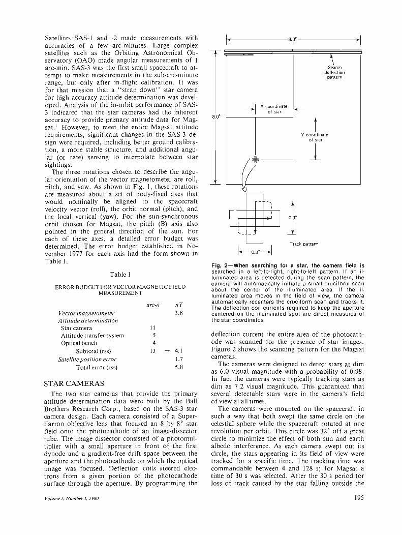
Satellites SAS-1 and -2 made measurements with accuracies of a few arc-minutes. Large complex satellites such as the Orbiting Astronomical Ob­servatory (OAO) made angular measurements of 1 arc-min. SAS-3 was the first small spacecraft to at­tempt to make measurements in the sub-arc-minute range, but only after in-flight calibration. It was for that mission that a "strap down" star camera for high accuracy attitude determination was devel­oped. Analysis of the in-orbit performance of SAS-3 indicated that the star cameras had the inherent accuracy to provide primary attitude data for Mag­sat. 1 However, to meet the entire Magsat attitude requirements, significant changes in the SAS-3 de­sign were required, including better ground calibra­tion, a more stable structure, and additional angu­lar (or rate) sensing to interpolate between star sightings.

The three rotations chosen to describe the angu­lar orientation of the vector magnetometer are roll, pitch, and yaw. As shown in Fig. 1, these rotations are measured about a set of body-fixed axes that would nominally be aligned to the spacecraft velocity vector (roll), the orbit normal (pitch), and the local vertical (yaw) . For the sun-synchronous orbit chosen for Magsat, the pitch (B) axis also pointed in the general direction of the sun. For each of these axes, a detailed error budget was determined. The error budget established in No­vember 1977 for each axis had the form shown in Table 1.

Table 1

ERROR BUDGET FOR VECTOR MAGNETIC FIELD MEASUREMENT

arc-s nT Vector magnetometer 3.8 A ttitude determination

Star camera II Attitude transfer system 5 Optical bench 4

Subtotal (rss) 13 4.1

Satellite position error 1.7

Total error (rss) 5.8

STAR CAMERAS The two star cameras that provide the primary

attitude determination data were built by the Ball Brothers Research Corp., based on the SAS-3 star camera design. Each camera consisted of a Super­Farron objective lens that focused an 8 by 8 0 star field onto the photocathode of an image-dissector tube. The image dissector consisted of a photomul­tiplier with a small aperture in front of the first dynode and a gradient-free drift space between the aperture and the photocathode on which the optical image was focused. Deflection coils steered elec­trons from a given portion of the photocathode surface through the aperture. By programming the

Volume I , Number 3, 1980

If-o"'f---------8.00 ----------l,.~1

s~rch deflection

pattern

--1 X coo rdinate ~ of star

l Y coo rd mate

of star

cjJ 1 "-----,(f

~

T 0.30

I

'- - 1 Track pattern

Fig. 2-When searching for a star, the camera field is searched in a left·to·right, right·to·left pattern. If an il· luminated area is detected during the scan pattern, the camera will automatically initiate a small cruciform scan about the center of the illuminated area. If the il· luminated area moves in the field of view, the camera automatically recenters the cruciform scan and tracks it. The deflection coil currents required to keep the aperture centered on the illuminated spot are direct measures of the star coordinates.

deflection current the entire area of the photocath­ode was scanned for the presence of star images. Figure 2 shows the scanning pattern for the Magsat cameras .

The cameras were designed to detect stars as dim as 6.0 visual magnitude with a probability of 0.98. In fact the cameras were typically tracking stars as dim as 7.2 visual magnitude. This guaranteed that several detectable stars were in the camera's field of view at all times.

The cameras were mounted on the spacecraft in such a way that both swept the same circle on the celestial sphere while the spacecraft rotated at one revolution per orbit. This circle was 32 0 off a great circle to minimize the effect of both sun and earth albedo interference. As each camera swept out its circle, the stars appearing in its field of view were tracked for a specific time. The tracking time was commandable between 4 and 128 s; for Magsat a time of 30 s was selected. After the 30 s period (or loss of track caused by the star failing outside the

195

camera's field of view) , the camera was com­manded to break lock and search for another star. In this manner a "snapshot" of stars was located in the camera field of view.

Like most real devices the camera outputs were not truly linear or independent. As a result there were variations from an idealized linear response of several arc-minutes. The camera's ultimate ac­curacy was achieved by calibrating these effects during ground tests and removing them during post-flight data processing. Each observed position, once these effects were removed, was accurate to 10 arc-s or better with respect to the camera optical axis.

ATTITUDE TRANSFER SYSTEM The transfer of each observed star position to the

vector magnetometer depended on the accuracy of the attitude transfer system (ATS). The system, built by the Barnes Engineering Corp., measured the relative orientation of the vector magnetometer with respect to the star cameras via two optical systems that measured the rotational angles of pitch, yaw, and roll. Both optical systems used a 125 Hz, 50070 duty cycle, modulated infrared beam at 930 nanometers to perform the optical measure­ment. This allowed both optical filtering and a syn­chronous detection scheme to eliminate effects of interfering light sources such as sun or earth albedo.

The simplest system was one that measured the pitch and yaw angles of the vector magnetometer with respect to the optical bench . The pitch/ yaw transceiver generated at the transceiver exit pupil a 1.8 cm square beam that was reflected by the flat mirror mounted on the vector magnetometer plat­form. The return beam formed a square image in the focal plane of the transceiver 0.03 cm on a side. When perfectly collimated, the image was centered on two split detectors as is shown in Fig. 3. Pitch or yaw rotations of the vector magnetom­eter platform produced displacements of the image. The two detectors were oriented so that, to first order, the pitch sensor was insensitive to yaw mo­tion and the yaw sensor was insensitive to pitch motion . A 1 arc-s rotation in either pitch or yaw produced displacement of the image on the order of 1.3 x 10 - 4 cm, which generated an output in the appropriate split detector. The maximum angular rotation, allowed to keep the pitch/ yaw system within its linear region, was ±3 arc-min. A second constraint on the pitch/ yaw system was the allowable translation of the vector magnetometer. If the flat mirror translated more than ± 1.9 cm, the collimated beam would be vignetted or possibly not returned to the pitch/yaw transceiver.

The roll system was much more complicated. It was, in essence, trying to measure the rotation (twist) about the line of sight of the optical system. The measurement was made by generating an off-

196

Main beamsplitte r

Light from objective lens

Yaw detector

Sp lit detectors

Beam image& in focal plane ~

Pitch detector

Compensation detector

~Beam image ~ in focal plane

Compensation reticle

Fig. 3-The light-emitting diode (LED) of the attitude transfer system generates an infrared signal that is formed into a square image by the LED mask at the focal plane of the objective lens. The source beamsplitter diverts a small amount of the transmitted and received energy to the compensation and automatic gain control detectors, which stabilize the sensor performance. The majority of the returned signal is diverted to the pitch and yaw detectors by the detector beamsplitters. There the image formed by the LED mask is focused on the two silicon cells in each detector. Yaw motion causes the beam image to move along the horizontal axis of each de­tector, producing a change in the differential output of the yaw detector while leaving the output of the pitch de­tector unchanged. Pitch motion causes the image to move along the vertical axis of the detector, producing change in the output of the pitch detector.

axis collimated beam that produced a pseudo-yaw signal as a function of roll rotations. The roll opti­cal system is illustrated in Fig. 4. A transceiver was located on the optical bench but was displaced from the roll axis. The collimated signal was trans­mitted to a dihedral mirror on the magnetometer platform that reflected the beam to a second dihe­dral mirror on the optical bench. From this base dihedral mirror the beam was reflected back on it­self to the transceiver.

In its simplest form the dihedral mirror on the magnetometer platform can be thought of as re­flecting the transmitted image onto a circle whose radius is defined by how far the transceiver is off the roll axis. As the magnetometer dihedral mirror rotates, the transmitted image moves around the circle, producing a pseudo-yaw motion. In fact, the two dihedral mirrors could be flat mirrors tilted at the appropriate angles and produce the same result, but both pitch and yaw motion of the magnetom­eter would corrupt the roll measurement. The dihe­dral mirrors are insensitive to rotations about the ridge line. Thus the dihedral mirror on the magne­tometer platform effectively decoupled yaw from the roll measurement and the decoupled pitch mo­tion of the base dihedral mirror .

The transmitted roll image was focused onto another split detector in the transceiver that de­tected the pseudo-yaw motion . In this case, how-

johns H opkins A PL Technical Digest

Roll

~~:;';:~4Sr---Dihedral ridge line

Light

sensor

Imagey~h

- - - - -./ "'Base dihedral

mirror

Fig. 4-The roll system transceiver generates a colli· mated beam that is reflected by the magnetometer dihe· dral mirror. As the dihedral mirror rotates about the roll axis, the reflected beam traces out a circle in the pitch/yaw plane. The base dihedral mirror causes the reflected beam to be returned to the transceiver when the magnetometer dihedral ridge line lies in the roll/yaw plane. For small roll rotations, the returned image is translated parallel to the pitch axis (as a yaw rotation would produce in an autocollimator), which is measured by the split detector.

ever, the pseudo-yaw motion for a 1 arc-s roll rota­tion was only 1 X 10 - 5 cm. In addition, because the roll rotation appeared as a yaw motion, actual yaw rotations between the transceiver and the base dihedral mirror appeared as roll motion and, un­fortunately, at an even more sensitive level than the true roll rotation. This put a very stringent require­ment on the Magsat optical bench and required the rotation about the line connecting the transceiver and the base dihedral (yaw) in the plane of the bench to be less than 0.2 arc-s if such motion was to affect the roll measurement by less than 2.5 arc-so This effect was noted during ground calibra­tion of the roll system. Measurements taken with the spacecraft in two configurations that reversed gravity-induced distortion in the optical bench pro­duced significant changes in the roll output. This 1 g bias was removed by the roll system calibra­tion.

PRECISION SUN SENSOR The precision sun sensor (see Figs. 5 and 6),

manufactured by the Adcole Corp., was the only primary attitude sensor that was sufficiently clean

Volume 1, Number 3, 1980

c

I

c A periodic pattern reticle

B periodic pattern reticle

A coarse reticle

B B coarse reticle

-A

Fig. 5-The precision sun sensor resolves the orientation of the sun line into two angles (ex and (3) in the sensor coordinate system by means of the A and B reticle assemblies. The periodic patterns determine the ex and {:3 angles with a precision of 2 arc·s in a 2.2' repeating pat· tern. The coarse reticles determine which one of the 2.2' segments (in the 32' field of view) actually contains the sun line.

Fig. 6-The periodic pattern reticle assemblies consist of two thin, fused, silica plates separated by a fused silica spacer. Four photocells are located beneath the bottom plate. A periodic grating deposited on the lower surface of the top plate has equal·width lines and spaces with a grating period w. The bottom plate has four identical periodic patterns deposited on the upper sun·facing sur· face, with the same grating period as the upper plate. However, each of these four lower patterns is displaced by one-quarter of the grating period. When combined, these four periodic patterns form a 4·phase filter for light reaching the photocells beneath the four patterns.

197

magnetically to be mounted near the vector magne­tometer. The sensor optical system resolved the angle between the sun line and a sensor coordinate system into two angles with a resolution of better than 2 arc-s and an accuracy of 12 arc-s root mean square (rms) based on preflight calibration. The sensor optics contained two reticle assemblies for each angle measurement. Each assembly consisted of one periodic pattern reticle and one coarse angle reticle. The periodic pattern reticle provided angu­lar information with 2 arc-s resolution over re­peated angular periods of 2.20. The coarse angle reticle determined which of the periodic patterns the sun line was in over a range of ± 32 0 •

The periodic pattern reticle acted as a 4-phase filter for the incident sunlight with a spatial distri­bution of intensity. The position of the intensity distribution, and consequently the amount of light transmitted by the 4-phase grating to the photo­cells, was a function of the sun angle. As the sun angle moved in the plane perpendicular to the grat­ing lines, the output of each of the 4 photocells varied sinusoidally with a period of 2.20 and with each cell in phase quadrature. The sensor electron­ics converted the photocell outputs to digital data.

By combining the periodic pattern reticle outputs with the coarse pattern reticle outputs, which un­ambiguously determine the angles ex and (3 with a resolution of 1 0

, the sun angle could be determined with a resolution of 2 arc-so

Like most other highly accurate sensors, small imperfections in the system created nonlinearities in the actual sensor output. For the sun sensor, these nonlinearities were caused by a number of factors such as the flatness of the grating substrates, the photocell spectral response, the skew (misalign­ment) between the input and output gratings, and the thickness of the grating patterns. Analysis by the Adcole Corp. resulted in a transfer function de­pendent on higher order harmonics of the fine reti­cle period that reduced the errors to the level of 12 arc-s rms.

Fig. 7-The Magsat optical bench shown here was fabri· cated by the Convair Division of General Dynamics. The inclined planes on the top surface hold the star cameras. The ATS components are mounted on the underneath side as illustrated in Fig. 1. The silver-like surface of the struc­ture is the aluminum moisture barrier.

198

OPTICAL BENCH REQUIREMENTS

For the ADS to function, the attitude sensors had to be connected by means of extremely stable struc­tures. The spacecraft optical bench (Fig. 7) and the magnetometer platform were designed and built to hold the alignment of the system elements mounted on them to deflections of 1 to 2 arc-s during orbital operations. In addition, they could suffer no align­ment changes during the launch and prestabiliza­tion phases of the mission. Severe weight con­straints, in conjunction with the thermal, struc­tural, and magnetic requirements, led to the choice of graphite-fiber reinforced epoxy (GFRE) for the construction of both structures. Active temperature control was necessary to meet thermal deflection objectives. The optical bench was attached to the spacecraft by means of a kinematic mounting ar­rangement to prevent significant deflection caused by spacecraft bending.

The selected material was superior to the other materials (such as aluminum or beryllium) in strength and stiffness ratios and in coefficient of thermal expansion, and it is not magnetic. It has some unique properties that require special care but are tractable. GFRE consists of graphite fibers lying in a single plane, held together by resin. The desir­able properties of GFRE exist only in the fiber plane. Normal to the plane, the thermal properties of GFRE degrade, approaching those of epoxy. By using an egg crate construction technique degrada­tion of the anisotropic properties was reduced.

Another factor considered was hygroscopicity. Strains caused by water absorption by GFRE during satellite construction and testing can approach 100 {(m/m and can produce deformations far exceeding those caused by thermal sources. Critical align­ments of bench-mounted components, performed when the bench had a high moisture content, were likely to change in orbit as the moisture was re­leased in vacuum. This undesirable property was reduced to tolerable levels by the application of a moisture barrier to the external surfaces of the op­tical bench. The moisture barrier consisted of 0.017 mm aluminum foil bonded to the GFRE.

A comparison of the critical alignment goals and the expected thermal deflections of the satellite structure when in orbit indicated that the bench should be attached to the structure in a manner that would not introduce bench bending. This anal­ysis led to a kinematic arrangement for attaching the bench to the spacecraft. Of the three attach­ments, one restricted all three translational degrees of freedom and the other two restricted the three rotational degrees of freedom without introducing additional translational constraints.

Even with the use of GFRE, the requirement for temperature control was reasonably stringent. For the optical bench, which was 3.8 cm thick and had a maximum separation between any two compo­nents of 66 cm, a temperature gradient through the

fohns Hopkins APL Technical Digesl

bench of 0.5°C would produce a deflection of 1 arc-so In addition to controlling the bench tempera­ture, -it was necessary to maintain each of the bench-mounted components at a constant tempera­ture. The basic approach taken was to prevent large temperature gradients by minimizing heat flow within the bench. The bench was first en­closed in its own multilayer thermal blanket within the spacecraft to reduce heat transfer by radiation to its surroundings. Second, the five components and three mounting points that must penetrate the blanket were heated to 25.0 ± 0.2°C. Third, ther­mal connections between the bench and the heater­controlled surfaces had relatively high thermal re­sistance.

The three spacecraft attachment fittings were de­signed to minimize heat flow between the bench and the spacecraft structure by controlling the tem­perature to 25 0 C through the use of thermostati­cally controlled heaters. Thermal resistance in­troduced between the bench and the spacecraft re­duced the required heater power substantially. Also, in those few cases when the temperature of the structure was greater than 25°C, the heat flow into the bench was limited by the resistance.

Because the optical components (i.e., the two ATS optical heads, the base dihedral mirror, and the two star cameras) have direct heat leaks to space, they had to be directly controlled to the de­sired temperature. In addition, they had to be mounted so that precise alignment was maintained through all mission phases. Thus titanium, a mate­rial with low thermal conductivity, was used for the joints between the bench and each component. A heater placed directly on the bottom of each com­ponent served the dual function of preventing heat flow from the bench and controlling the compo­nent's temperature. This design resulted in a bench with minimal thermal gradients through and across the bench. Post-launch data show that gradients were less than 0.1 ° C.

SYSTEM VERIFICATION AND PERFORMANCE

The Magsat attitude determination system was a composite of individual units that had to be assem­bled into a calibrated system. Each of the sensors was tested and calibrated by its manufacturer to various levels depending on the manufacturer's fa­cilities and the ability of that particular component to operate without assembly into the spacecraft. Verification of the primary attitude system was per­formed at the Calibration, Integration, and Align­ment Facility at the NASA/Goddard Space Flight Center. Tests were performed to determine the alignments of the star cameras and the ATS com­ponents to an optical reference mounted on the spacecraft optical bench. The star camera calibra­tion algorithms generated by the Massachusetts In-

Volume 1, Number 3,1980

stitute of Technology's Center for Space Research, based on the calibration data furnished by the Ball Brothers Research Corp., were verified. The cali­bration of the ATS system related the sensor out­puts to the angular relationships between the space­craft optical bench reference cube and a reference cube on the vector magnetometer (see Fig. 1). The alignments between the precision sun sensor and the vector magnetometer were also measured at this time, but no verification of the Adcole calibration of the sun sensor was performed.

The flexure induced in the bench by the weight of the components was measured by making all alignment measurements with the spacecraft B axis both up and down (i.e., ± 1 g). The measurements indicated that star camera No. 1 moved 9 arc-s and star camera No. 2 moved 30 arc-s because of weight reversal. The ATS pitch/yaw system moved less than 3 arc-s, but the roll system changed by 70 arc-s because of the sensitivity of the roll output to yaw rotation between the roll transceiver and the base dihedral mirror. Changes of 10 arc-s in the sun sensor alignment were measured when the vec­tor magnetometer plate assembly was flipped to re­verse the weight loading. The final calibration of the system used these measured changes to deter­mine the relative alignments when in space. The weight loading effect was removed by averaging the difference in alignment in the ± 1 g cases.

A second set of alignment measurements was made after the spacecraft had been exposed to en­vironmental testing. Residual changes caused by en­vironmental stress were less than 3 arc-s for the ATS and star camera No.2. Changes in star camera No.1 were slightly larger, reaching 10 arc-so

The data from the various attitude sensors were used as inputs to a computer program developed by the Computer Sciences Corp., that generated three­axis attitude information at 0.25 s intervals. 2 The program computed the attitude for each 0.25 s in­terval based on the sensor data available. If both cameras were tracking identified stars, the magne­tometer orientation was computed using the two star sightings and ATS data. If only one star camera was tracking an identified star, the second vector required for an attitude solution was derived from the sun sensor data. If neither star camera was tracking an identified star, a motion model was used to interpolate between valid star tracks. This motion model determined the right ascension and declination of the B axis from sun sensor data and the rotation (pitch) about the B axis by integrating the output of the pitch axis gyro.

The attitude determination program was capable of making certain self-consistency checks to ascer­tain the validity of the data and the stability of the system throughout the mission. One major check was the determination of biases in the system from data sets in which all three sensors generated valid data simultaneously. These bias determinations, computed from data taken early in the mission, in-

199

dicated that the two star cameras were within 6 arc­s of the prelaunch alignment measurements . Differ­ences between the attitude as computed by the star cameras, the A TS, and the sun sensor were larger than expected (based on ground testing). Since the star camera alignment did not appear to have changed, the discrepancy appeared to lie either in the A TS or the sun sensor. Further analysis, using a least squares fit of the observed magnetic field data, determined the distribution of the error. The best fit of the data to a model of the earth's field indicated that the major discrepancy of 200 arc-s in roll was due to the ATS (i.e., the precision sun sen­sor measures the roll angle correctly). Likewise, a smaller yaw discrepancy of 55 arc-s was associated with the sun sensor. The sources of these errors in the individual instruments have not been deter­mined .

In time, the input of each sensor varied over a large portion of its range; i.e., the sun moved in a circle about the B axis during each orbit of the spacecraft, the ATS angles varied, and many stars were tracked over the entire field of view. During such a period of time, variation in the difference

200

between a reference vector (determined by star camera No.2, the ATS, and the sun sensor) and the same vector determined solely by star camera No. 1 was computed to be 5 arc-s root mean square (rms) .3 This variation was a measure of the system noise and the ability of all sensor transfer functions to remove the system nonlinearities.

Computations of system biases were performed several times during the mission life. Variations in system alignments were small, but with some drift that was correlated with temperature changes. A failure of the heater on one of the star cameras in December 1979 caused a shift of 6 arc-s o The data set of attitude measurements for the Magsat mis­sion has good internal consistency and, with resolu­tion of the observed bias, the system has an ab­solute accuracy of 20 arc-s rms .

REFERENCES JR . L. C1eavinger and W. F. Mayer , "Attitude Determination Sensor for Explorer 53." AIAA Paper 76-114, Proc. 14th Aerospace Science Meeting (1976).

20. M. Gottlieb et al., MAGSA T Fine Aspect Baseline System Overview and Analysis, Computer Science Corp. Document CSC SO - 78 - 6067 (1978).

3F. Van Landingham , personal communications (March 1980).

Johns Hopkins APL Technical Digest

JAMES F. SMOLA

THE MAGSAT MAGNETOMETER BOOM SYSTEM

The boom connecting the sensor platform with the Magsat spacecraft provided position and tilt adjusting capabilities for the remote mirrors referenced to the vector magnetometer. Once set in orbit, the mirror positions were to be maintained passively. Only vanishingly small angular deviations caused by thermally and dynamically induced structural distortions were permissible, which made the design and test problems extremely difficult.

INTRODUCTION The need for a simple, extendable, lightweight,

precisely alignable, virtually distortion-free struc­ture for Magsat, capable of overcoming the stiff­ness of sizable multiconductor electrical cabling, presented a most difficult design requirement. The critical requirement was the need to position with precision magnetically sensitive instruments at a considerable distance from sources of magnetic contamination in the spacecraft. The problem was particularly acute because the magnetometer sen­sors were designed to measure a 60,000 nanotesla (1 nT = 10-9 weber per square meter) magnetic field with a precision of ± 1 nT.

Very ' precise knowledge of the vector magnetom­eter sensor's angular orientation was important. Because of the extremely narrow bandwidth of the attitude transfer system (ATS) , which measured the angular orientation of the magnetometer, special

Magnesium end fitting Graphite epoxy link

Length-indicating potentiometer

Boom caging T -rod

SP caging rod

precautions were taken to control thermal distor­tions, mechanical misalignments, and dimensional instabilities in the design of the structural system that supported the sensors and separated them from the spacecraft instrument section.

SYSTEM DESCRIPTION The magnetometer boom system consisted of a

14-link scissors boom, a 3-axis gimbal, and the sen­sor platform (see Fig. 1). The platform was con­nected to the instrument module electrically with multiconductor cabling that was routed through the interior of each boom link. Two independent, py­rotechnically actuated caging systems were used during launch to contain and protect the boom and platform in their stowed configurations . The 3-axis gimbal located at the boom base provided the boom with pitch, yaw, and roll capabilities of ±2,

Thermistors

Alignment guide

Pitch gimbal actuator

Fig. 1-Magnetometer boom system (partially extended).

Volume I. Number 3.1980 201

±2, and ±5°, respectively, for acqulSltlOn of the ATS. The drivers for each gimbal actuator, con­sisting of a 491-Hz square-wave inverter powering two phase-synchronous hysteresis gear motors cou­pled to gearboxes, provided average pitch, yaw, and roll scan rates of 30 arc-sis. A pair of tension springs attached to the drive base and the instru­ment module structure eliminated all unrestrained play in the gimbal actuator adjusting screws. Rota­ry potentiometers geared to the output shafts of each of these gearboxes were calibrated to give the angular orientation of the drive base.

The boom drive consisted of a right- and a left­handed ball screw that was rotated by a fourth, inverter-driven, synchronous hysteresis gear motor. A rotary potentiometer geared to the output shaft of the gearbox was calibrated to indicate boom length during deployment. Confirmation of total extension was given by a second potentiometer made of nonmagnetic materials and pinned to one of the boom hinges closest to the platform. Total deployment time was about 20 minutes.

Weight and thermal distortion dictated the use of graphite-epoxy material for the boom links. The basic link was 94 cm long and 1.07 X 5.08 cm in cross section . Magnesium fittings were fastened to the ends and the center of each link with semirigid epoxy to prevent interface cracking caused by dif­ferential expansion. Each link was a hollow box with a 0.076 cm thick wall and was covered inter­nally and externally with an aluminum foil mois­ture barrier to control moisture absorption and desorption - sources of dimensional instability -in the inherently hygroscopic graphite epoxy. A final wrapping of aluminized Kapton coated with aluminum oxide was added for temperature con­trol. The links were hinged to each other with pins that were forced through compliant undersized bushings. This permitted rotation but eliminated all unrestrained mechanical side play.

The aluminum-foiled, graphite-epoxy platform was attached to the tip of the boom through a hollow graphite-epoxy box-like spacer and a "figure-eight" mechanism that enabled the plat­form to translate while maintaining its attitude nor­mal to the boom axis as the boom extended. At­tached to the platform with a kinematic suspension was the temperature-controlled vector magnetome­ter base, which in turn had attached to it the vector magnetometer sensor, the remote plane and dihe­dral ATS mirrors, and a precision sun sensor. The kinematic suspension provided a compliant mount for the magnetometer base and isolated it from thermally induced structural distortions that would be detrimental to the alignment of the vector mag­netometer and the remote mirrors. The scalar mag­netometer was attached to a 1.27 cm thick epoxy­glass thermal isolator that was fastened to the side of the graphite-epoxy spacer.

The weight breakdown for the boom system is shown in Table 1.

202

Table 1

WEIGHTS OF BOOM SYSTEM COMPONENTS (kg)

Link structure 2.72 Drive assembly 2.93 Gimbal actuators (3) 3.09 Caging subsystems 1.13

Inverters (2) 0.62 Electrical subsystem 0.76

Sensor platform assembly 7.03 Boom cable 2.72

Total weight

9.87

1.38

9.75

21.00

OPERATIONAL REQUIREMENTS Magnetic contamination of the magnetometer

sensors was avoided by locating the star cameras (which were magnetic) on an optical bench in the spacecraft instrument module. (Since the potential for magnetic contamination of the sensors was so great, the urge to locate the cameras on the sensor platform was dispelled well in advance of any serious design effort.) On command, the boom was to uncage and displace the sensor platform 6 m away from the instrument module. To satisfy re­quirements imposed by the ATS, which measured the vector magnetometer tilt relative to the star cameras, the boom was to maintain the platform position so that the center of a plane mirror, pre­cisely attached to the backside of the vector magne­tometer sensor, remained within a ± 1.91 cm square target zone. This zone was centered on the axis defined by an infrared light beam emanating from an A TS optical head located in the instrument module. The plane mirror had to remain orthogo­nal to the optical axis within 3 arc-min; this turned out to be the greatest challenge.

AREAS OF MAJOR CONCERN Although the precision scissors boom was a

flight-proven concept, the remote, precisely aligned platform was not. Concern over magnetic interfer­ence disallowed electrically powered adjusting mechanisms at the platform end. Consequently, tilt adjustments could only be achieved by gimbaUing the boom at its base, which would cause the plat­form to translate. This side effect, coupled with the narrow field of view of the ATS, severely limited the tilt adjusting capability. For this reason con­siderable engineering analysis and testing were necessary to demonstrate that the Scout launch en­vironment, uncaging, deployment, thermal distor­tions, and attitude control disturbances would not compromise the ability to achieve the precise align­ments that were required.

Johns Hopkins APL Technical Digest

The following three major areas of concern re­ceived considerable attention.

Control of Thermal Distortion The requirement was to limit initial boom ther­

mal distortions caused by broadside solar illumina­tion sufficiently to permit acquisition of the ATS remote mirrors by gimballing the boom at its base. Although the gimbals were adjustable ±2° in pitch and yaw and ± 5 ° in roll, any tilting of the boom at its base would translate as well as rotate the remote mirrors . Since the target zone was ± 1.91 cm square, any mirror tilting that was necessary for acquistion had to be achieved within 0.33 ° once the mirrors entered the target zone. This made the ini­tial tilt angle of the mirrors and direction of tilt ex­tremely important. If, for instance, the mirrors were perfectly centered within the target zone ini­tially, acquisition would have to be achieved within 0.16° or 9.6 arc-min of angular displacement.

The ±3 arc-min requirement on mirror angle limited the permissible transverse offset of boom tip position to ±0.51 cm for simple mechanical misalignment and ±0.25 cm for misalignments caused by thermal distortion . It was important for the system to be free of play and for the boom ele­ments to be made of some material that is virtually immune to thermal distortion. (Active temperature control was ruled out because of the complexity re­quired for implementation and lack of sufficient electrical power.) Graphite fiber-reinforced plastic (graphite epoxy) with a coefficient of thermal ex­pansion of very nearly zero (+0.34 x 1O - 6rq was chosen to cope with the thermal distortion pro­blem.

To control boom-link temperatures and tempera­ture gradients in the presence of the solar and earth infrared environments, each link was taped with aluminized Kapton coated with aluminum oxide. This thermal covering was selected to give link equilibrium temperatures close to 25 ° C where all mechanical alignments would be checked .

Thermal distortion tests conducted in the God­dard Space Flight Center simulator on a four-link version of the flight boom yielded favorable results and indicated that the transverse and angular dis­placements of the platform caused by boom ther­mal distortion would be well within the allowable range.

U ncaging, Separation, and Extension Two independent caging systems were provided

to contain the boom during launch and to prevent the 7 kg sensor platform from transmitting damag­ing loads into the relatively delicate boom struc­ture. Both were actuated by pyrotechnic piston-type actuators. Because the boom system was stowed in an unheated external compartment, boom-link and cable temperatures as low as -70°C were expected. Resistive heaters attached to the boom drive base

Volume I, N umber 3,1980

were to provide 16 W of power to warm the boom cable and drive just prior to platform separation and boom extension. Torsion springs located at each boom-link pivot were designed to overcome cold-cable stiffness as well as hinge frictional resistance. The existence of many single-point failure mechanisms in this area of concern resulted in a considerable amount of cold temperature testing to demonstrate and guarantee system in­tegrity.

Pre-Launch Mechanical Alignments To bring the remote mirrors mounted on the sen­

sor platform into the fields of view of the ATS pitch/yaw and roll optical heads and then into linear range by fine adjustment , a terrestrial test that negated the 1 g bias had to be contrived . The best proposal utilized a pair of 6.1 m long water troughs (Fig. 2) . Specially designed float s with gim­balled pulleys were attached to each of the boom­link pivots. The idea was to simulate a zero-g con­dition in a plane parallel to the plane of the water . Remote mirror transverse or angular offsets could then be corrected by gimballing the boom at its base or introducing shims at the platform interface. The boom system was installed in a special fixture that was attached to a rotary table, the purpose of

Fig. 2-The Magsat magnetometer boom float system. The magnetometer boom is suspended from floats in 6.1 m long flotation tanks that provided zero-g simUlation in the horizontal plane. The boom was rotated about its longitudinal ax is into four positions 90° apart. Measurements of inclinations of sensor platform­mounted mirrors provided data that were used to align the mirrors by operating the gimbal at the base of the boom or by shimming the vector magnetometer base at the sensor platform end. Final measurements, adjust­ments, and checks were made by the attitude transfer system with the instrument module mounted on the ro­tary fixture.

203

which was to rotate the boom into its pitch and yaw planes for orthogonal plane, zero-g measure­ments, and adjustments. With the aid of an autore­flecting telescope, a theodolite, and numerous mir­rors to measure the transverse and angular offsets of the plane remote mirror, sufficient data were obtained to guarantee remote mirror acquisition in orbit.

OPERATIONAL PERFORMANCE On November 1, 1979, following a successful

launch a few days earlier, the spacecraft attitude was stabilized. At 6:27:53 PM EDT, after successful uncaging, the magnetometer boom was extended. Telemetry indicated that the extension was proper and complete (see Fig. 3 of the Mobley article in this issue). Surprisingly, telemetry indicated that the remote mirrors were within the field of view of the ATS optical heads. This obviated the need for extensive gimbal searching for ATS acquisition. On the following day slight gimbal adjustments were made to bring the remote mirrors into the ATS lin­ear range. Subsequent gimbal adjustments were un­necessary.

Figure 3 - data from one orbit 92 days into mission life - shows roll, pitch, and yaw angles relative to orbital time and boom-link temperatures as measured by thermistors attached directly oppo­site one another on a boom link. Oscillations are evident, with periods approximately equal to the orbital period and amplitUdes well within the ± 180 arc-s pitch and yaw and ±300 arc-s roll limitations of the ATS. The boom-link temperatures exhibit

204

Acquisition ranges: Pitch/yaw ±1S0 arc·s; Roll ±300 arc-s Nominal: 0 arc-s

20,--.---,--,---,--,---,--,---,---,--, '" ~ o -- ------~ -20 ~ -40 R2!L - __

",1ij -60 -- "-~ e -SO Pitch

.~ -100 -120

-----., .,

".­,/

u -"'~ 44

~----Orbital period: 92.S min-------;~~I

~ ~ 40I--S_u_n_sid_e_Design temperature bandwidth: 25°C ±10°C

Eo ~ 36 ....... ---o " Darkside en E 32

e 0~~---L--~--~~--~--~--S~0---L~100

Time (min)

Fig. 3-Magsat ATS remote mirror angles and magnetom­eter boom-link temperatures, 029:22:40:15 (January 29, 1980, orbit 1410).

this same cyclical characteristic. This coincidence leads to the inference that the boom is being ther­mally excited at the orbital frequency. The contin­ually varying temperatures are caused by the once­per-orbit coning of the solar vector. Their magni­tudes are functions of the boom-link angle relative to the sun, which is set by the link angle relative to the boom axis and the seasonal variation in the solar vector.

The landmark performance of the boom system in orbit is an endorsement of the concept and of the special precautions that were exercised to guarantee its successful use.

Johns Hopkins APL Technical Digest

WINFIELD H. FARTHING

THE MAGSAT SCALAR MAGNETOMETER

The Magsat scalar magnetometer is derived from optical pumping magnetometers flown on the Orbiting Geophysical Observatories. The basic sensor, a cross-coupled arrangement of absorption cells, photodiodes, and amplifiers, oscillates at the Larmor frequency of atomic moments pre­cessing about the ambient field direction. The Larmor frequency output is accumulated digitally and stored for transfer to the spacecraft telemetry stream. In orbit the instrument has met its principal objective of calibrating the vector magnetometer and providing scalar field data.

INTRODUCTION The cesium vapor optical pumping magnetometer

used on Magsat is derived from the rubidium mag­netometers flown on the Orbiting Geophysical Ob­servatories (OGO) between 1964 and 1971. The Polar Orbiting Geophysical Observatories (Pogo) used rubidium-85 optical pumping magnetometers, I while those on the Eccentric Orbiting Geophysical Observatories (Eogo) used the slightly higher gyro­magnetic ratio of rubidium-87.

Data generated by the Pogo instruments pro­vided the principal data base for the U.S. input to the World Magnetic Survey, 2 an international co­operative effort to survey and model the geomag­netic field . It is partly this body of data that under­lies the most accurate analytical models of the main geomagnetic field in present use. 3 Further studies of the Pogo data base and other sources led to the recognition of the need for a dedicated mission, such as Magsat, to increase the resolution for crustal studies, to incorporate vector measure­ments, and to correct the models for secular varia­tion.

When considering various options for implement­ing a scalar magnetometer for use in space, optical pumping instruments are clearly superior in view of requirements for accuracy, dynamic range, infor­mation bandwidth, ease of data collection and stor­age, power and weight requirements, and reliabil­ity. For the self-oscillating type used in OGO and Magsat, cesium-133 is superior to other alkali va­pors because of its narrower resonance line width, followed by rubidium-87 and rubidium-85. When instrumentation for Pogo was selected, cesium had not been used extensively in magnetometry and thus was not considered sufficiently developed to use in spaceflight. Rubidium-87, with its higher gyromagnetic ratio, would have resulted in a wide range of frequencies over which it would have been difficult to control the electronic phase shifts that are so important to accuracy. Rubidium-85, with its gyromagnetic ratio of 4.66737 Hz per nanotesla

Volume 1, Number 3,1980

(nT), was therefore used even though, from the standpoint of resonance line width, it is the poorest of the three. In the interim between OGO and Magsat, cesium-133 came to be the most commonly used isotope in alkali vapor magnetometry and was thus the natural selection for Magsat.

PRINCIPLE OF SENSOR OPERATION The alkali vapor magnetometer is based on the

phenomenon of optical pumping reported by Dehmelt4 in 1957. The development of practical magnetometers followed rapidly, evolving in one form finally to the dual-cell, self-oscillating magne­tometer5 shown in Fig. 1. Two of these twin-cell magnetometers are combined in the Magsat magne­tometer. In each twin-cell sensor an electrodeless discharge lamp driven by the RF exciter produces resonance radiation that is collimated and passed through an interference filter, which selects the DI spectral line (894.5 nm for cesium-133) and rejects the D2 spectral line (852.1 nm for cesium-133). The light is then circularly polarized before it is allowed to optically excite cesium vapor contained in the absorption cells.

Two identical sets of optics are employed, with the direction of light propagation anti parallel, thus defining the "optical axis" of the system. The transmission of each absorption cell is monitored by a photodetector, amplified, and cross-fed back to solenoidal coils wound about the absorption cells coaxially with the optical axis. A closed loop is thus formed that oscillates if the loop gain is greater than unity at the frequency where the loop phase shift is zero. The frequency of oscillation is a direct measure of the strength of the ambient mag­netic field, i.e., the Larmor frequency of atomic magnetic moments precessing about the ambient field direction.

The modulation of light transmission obtained through application of a Larmor frequency signal to the solenoidal coil, termed the "HI" coil, results from transitions between the discrete hyper fine

205

Boom

Main body

L-------------------------------------+--fAA;m~pmlif~ie~rl-----~ Amplifier Output signal

Fig. 1-Dual·cell cesium magnetometer. The loop, composed of absorption cells, photocells, and amplifiers oscillates at a frequency proportional to the ambient field magnitude.

energy states that exist in the cesium atom when it is subjected to a magnetic field. The hyperfine splitting of cesium-I33 is shown in Fig. 2. Prior to the application of pumping light, the atoms can be considered to have a Boltzmann distribution among the energy states. Optical pumping polarizes the sample so that a nonequilibrium concentration of atoms in either the m (the Larmor frequency for transition) = + 4 or m = - 4 sublevel of the ground state is obtained, depending on both the sense of circular polarization and the direction of the optical axis component of the magnetic field .

Application of a (Larmor frequency) signal to the HI coil at the transition frequency for m + 4, + 3 (or m = - 4, - 3) causes the selective depumping of a group of atoms having a certain phase with the driving signal. Since the pumping probability depends on the angle to the light wave normal as the group of depumped atoms precesses, the light transmission is modulated at the Larmor frequency.

A single-cell absorption cell process is subject to "heading error" in that the Larmor frequency for transition m = + 4, + 3 differs from that for tran­sition m = - 4, - 3. The dual-gas-cell configura­tion has a strong advantage over single-cell magne­tometers in that the sense of circular polarization is such that when one cell is pumped to the m = + 4 state, the other is pumped to the m = - 4 state, resulting in a reverse skew for the two absorption cells. Since the dual-cell loop transfer function in­cludes the product of the individual absorption lines, a symmetrical two-cell composite line is ob­tained. Thus the frequency of operation should n()t change under reversal of the ambient field with respect to the sensor.

The frequency of oscillation of the loop is deter­mined by the open loop phase shift of all the com­ponents. If the net phase shift from all sources other than the absorption cells is zero at any fre­quency, the closed loop oscillates at the frequency where the phase shifts of the two absorption cells are equal and opposite. By the symmetry of the system, this frequency is the average of the eight

206

t D2 852.1 nm

fn = A Ho + Bn Ho2

A = 3.49847

B1 = -Ba = -93.5 B2 = -B7 = -66.7 B3 = -8 6 = -40.0 B4 = -Bs = -13.4

F=3-+-----------------------

62P1 /2

F=2·~~---------------------

m = +41 +3 I f1 (4 -+ 3)

D1 894.5 nm

2l F = 3

t21(f2 (3 -+ 2)

+1 If f3 (2 -+ 1) r--------_~::::::::::::::=-- 0 f4 (1 -+ 0)

-1 f fs (0 -+ -1) '" c W

F = 2

-2 ff6 (-1 -+ -2)

-3 ff f7 (-2 -+ -3) - 4 fa (-3 -+ -4)

-3 -2

'----_~§:==== -6 +1 +2 +3

Fig. 2-Energy diagram for cesium·133. Transition frequencies f1 to fa are in hertz for the applied field Ho in gauss (1 gauss = 105 nT).

absorption frequencies of the Zeeman spectrum for F = 3. This yields for the theoretical oscillation frequency

f = 3.49847 Ho ,

where f is given in hertz if the ambient field Ho is expressed in nanoteslas.

The various processes of modulating and moni­toring light in the twin-cell sensor are such that the loop gain depends on the product sin2 e cos e, where e is the angle between the optical axis and

Johns Hopkins APL Technical Digest

the applied field. Thus null zones are to be ex­pected in a twin-cell sensor when the ambient field is either along or perpendicular to the optical axis. These zones are termed "polar" and "equatorial" null zones, respectively. The Magsat magnetometer incorporates two such sensors, with their optical axes crossed at 55 0. The polar null zones are thereby eliminated because they have no intersec­tion, and the only remaining composite null zone is the intersection of the two equatorial null zones, shown in Fig. 3. In the Magsat magnetometer, the composite null zone is directed normal to the orbit plane, such that in normal operation in near-polar orbit the ambient field will never lie within the composite null zone.

It is desired, of course, to minimize the width of the null zones for each individual sensor. It is thus necessary to use high gain amplifiers in the system, the limitations being the noise level of the system and the requirement to maintain near-zero phase shift over the operating frequency range. The width of the null zones is also quite dependent on the operating temperature of the absorption cells. For cesium-133, the optimum cell temperature is 52°e. The four absorption cells in the Magsat magnetom­eter are maintained at the desired temperature by individual thermostatically controlled heaters. The heaters are made from bifilar-wound resistance wire to avoid magnetic signature, and each heater dissipates 0.5 W at 30 V when the thermistor-oper­ated control circuitry closes the circuit. The overall thermal environment is achieved by controlling sep­arately the beryllia yoke (into which the sensors are mounted) at 41°C, and enclosing the entire sensor in a passive thermal enclosure with a radiator whose area is selected to radiate the required amount of energy . Figure 4 shows the Magsat sca­lar magnetometer sensor configuration without its thermal enclosure or radiator.

DIGITAL DATA GENERATION Figure 5 is a diagram of the electronics necessary

to operate the sensors and to interface the space­craft telemetry system. In order to prevent inter­ference between the two sensors, they must be op­erated in frequency lock . This is accomplished by using a combining amplifier on one side of the sen­sors. The combining amplifier is repeated in order to implement fully the design objective of main­taining the maximum amount of redundancy for single sensor operation. The output signals from the two combining amplifiers are processed through completely independent signal processors consisting of phase-locked loop tracking filters, accumulators, and readout gates . In each signal processor chain, the bandwidth of the tracking filter is set at 25 Hz to ensure that the loop will track the varying input frequency adequately and to make negligible any errors associated with time lag in the closed-loop transfer function. The accumulators are of a com-

Volume I, Number 3,1980

I I

J- _ _ _

_ Nul l zone for sensor A Nul l zone f or sensor 8

+8 orbit

normal

_ Composite zone f or two dual-ce ll sensors

Fig. 3-Spatial coverage of the scalar magnetometer. The composite null zone, or intersection of the two individual sensor null zones, is oriented normal to the spacecraft or· bit plane. It should never contain the magnetic field vec­tor.

Fig. 4-Magsat scalar magnetometer sensor. Each cylinder contains optics and hybrid preamplifiers for one dual cell magnetometer. The central yoke is made of beryllia to minimize the temperature gradient. A flat beryllia radiator (not shown) is attached to the top of the yoke. The entire structure is housed in a fiberglass and multilayer thermal blanket enclosure.

mandable aperture type, a design feature that was incorporated to allow the sampled data to vary from the normal situation of a 30 ms aperture time (in which the information bandwidth is primarily that of the tracking filter) to a maximum aperture case (where the frequency characteristic of the sam­pling function is primarily determined by the aper­ture time and the resulting output data are substan­tially protected from frequency aliasing effects). In

207

Exciter A

Power bus A---"--~ Converter A

Exciter B \--------1 Filter board

Power bus B---~ Converter B

.---__ Aperture status A (8 bit)

r---'-----.,.....i-Aperture time A Sample A Bit clock A

\.-___ j<OII~Word gate A

Output data A

Frame sync Housekeeping data Word gate

Output data B

.----'L--~Word gate B Bit clock B Sample B

I....-_.,...-_ ........ ,...Aperture B

'---_Aperture status B (8 bit)

Regulated power r------,

Survival heater power

Fig. 5-Block diagram of scalar magnetometer electronics.

order to make this design objective compatible with resolution requirements, the tracking filters were designed to multiply the Larmor frequency by a factor of 16.

The output data word assigned to each scalar magnetometer data point. is 20 bits long. The last bit is made a parity bit, and the next to last bit was desired to be a data quality flag associated with that particular sample. This leaves 18 bits for the primary data sample, which was not compatible with the full range of commandable aperture times. Thus a pre scalar is included in each data processing chain. The prescalar is under the control of the commanded aperture time, which is delivered to the experiment in the form of a binary number, N, that specifies the aperture time as (2N + I)Tb, where Tb is the telemetry bit time of 0.512 ms. For N :;; 63, the prescalar factor, P, is 1. For 64 :;; N :;; 127, the prescalar factor is 2. For N ~ 128, the prescalar factor divides by 4.

The logic equation for the data quality flag, Q, associated with each data point is, for instance, for scalar A,

QA = TFA . (SIGA + SIGB) . (BRA + BRB) ,

where each term in the logic function has to be true over the accumulation time in which that particular data sample was collected. TFA = 1 means that the tracking filter associated with that data point was in lock throughout the accumulation time. SIGA + SIGB = 1 is a condition that the signal amplitude in either sensor A or sensor B is above a predeter­mined threshold throughout the accumulation inter­val. BRA + BRB = 1 is a condition that one or

208

both of the lamps must be operating within a pre­determined brightness range throughout the ac­cumulation interval. This form of the logic func­tion was selected in order to be compatible with the operation of both processing chains with a single sensor and yet to be an efficient rejector of a number of possible malfunctions within the instru­ment.

The sampling of each scalar is done at 4 samples per second, and the samples of scalar A and scalar B are interleaved to obtain a total of 8 equidistant samples per second.

OPERATION IN ORBIT The Magsat scalar magnetometer met its prin­

cipal in-orbit objective of calibrating the vector magnetometer and returned scalar field data, al­though intermittent noise in the lamp excitation cir­cuitry caused loss of lock in the tracking filters and, therefore, a reduction in the expected data rate.

Engineering data returned from the instrument verified that the thermal control circuitry per­formed as expected in controlling lamp and absorp­tion cell temperatures. Monitors in the lamp RF control loops were only reliable when the intermit­tent noise was absent but at such times showed that lamp A operated at control parameters identical to those observed during ground thermal-vacuum test­ing. Lamp B, which ran extremely efficiently dur­ing ground testing, required slightly more RF power in orbit. Sensors A and B were operated indepen­dently at times to serve as a cross check on ab­solute accuracy and to verify the integrity of the Larmor sensors.

Johns Hopkins APL Technical Digest

The lamp noise problem manifested itself dif­ferently in the two lamps. It first appeared in lamp A about 12 hours after the instrument was turned on and, except for a few periods after the lamp had been off for a day or more, was consistently present in the lamp excitation until the spacecraft entered the eclipse season, when a dramatic im­provement occurred. The problem was first ob­served in lamp B two weeks after turn-on and was present intermittently over a period of several hours in a way that has not been explained. Transi­tions from one state to another often occurred when one of the tape recorders was played back, but the problem was not associated with a par­ticular tape recorder. The lamp problem was most likely caused by a feedback mechanism to the spacecraft power that was not present to the same degree on the ground.

The effect of the interference on tracking filter lock was much more serious when the noise was present in lamp B. Thus the operational mode was to operate lamp A continuously and to operate lamp B approximately one day out of five in order

Volume 1, Number 3,1980

to fill in the A sensor null zones and to provide a more complete data set for calibration of the vector magnetometer.

Incorporation of the data quality flag in the out­put word proved indispensable to the rejection of data when the tracking filter was out of lock and enabled the combination of vector and scalar mag­netometers to meet substantially all the objectives, even in the presence of the lamp excitation noise.

REFERENCES IW. H. Fanhing and W. C. Folz , " Rubidium Vapor Magnetometer for Near Eanh Orbiting Spacecraft," Rev. Sci. 1nstrum. 38, pp. 1023 - 1030 (1967).

2A. J. Zmuda (ed.), The World Magnetic Survey, IAGA Bulletin No. 28 (1971) .

3Ibid., p. 148 . 4H. G. Dehmelt , Phys. Rev. 105 , p. 1487 (1957). 5 A. L. Bloom, " Principles of Operation of the Rubidium Vapor Magnetometer," Appl. Opt. 1, pp. 61 - 68 (1962) .

ACKNOWLEDGMENT - The Magsat scalar magnetometer was built for the NASA/ Goddard Space Flight Center by Bell Aerospace Systems Divisio n, Western Laboratories, and Varian Associates, Canada, Ltd. Mr. David Synder, BASD, was program manager for the project. The RF exciters were provided by Mr. L. J . Rogers of GSFC.

209

MARIO H. ACUNA

THE MAGSAT PRECISION VECTOR MAGNETOMETER

The Magsat preClSlon vector magnetometer was a state-of-the-art instrument that covered the range of ±64,OOO nanoteslas (nT) using a ±2000 nT basic magnetometer and digitally controlled current sources to increase its dynamic range. Ultraprecision components and extremely efficient designs minimized power consumption.

INTRODUCTION The instrumentation aboard the Magsat space­

craft consisted of an alkali-vapor scalar magnetom­eter and a precision vector magnetometer. In addi­tion, information concerning the absolute orienta­tion of the spacecraft in inertial space was provided by two star cameras, a precision sun sensor, and a system to determine the orientation of the sensor platform, located at the tip of a 6 m boom, with respect to a reference coordinate system on the spacecraft.

The two types of instruments flown aboard the spacecraft provided complementary information about the measured field. The scalar magnetometer measured the magnitude of the field independent of its orientation with respect to the sensor, with an absolute accuracy that ' is determined by atomic constants and thus is not subject to change as a function of time. On the other hand, the precision vector magnetometer measured the projections of the ambient field in three orthogonal directions with an absolute accuracy determined by calibra­tions with respect to a standard; thus they were subject to error and drift. Accuracy goals for the mission required a vector magnetometer capable of measuring the ambient field with a maximum error of ± 1 part in 64,000 in magnitude and 5 arc-s in orientation (1 arc-s = 0.00028°). The development of such an instrument within the constraints im­posed by the spacecraft represents a major techno­logical achievement that would have been impossi­ble without parallel developments in the areas of ultraprecise linear integrated circuits and miniature resistors. The design implemented for Magsat rep­resented an optimum compromise among many conflicting requirements and limitations imposed by available resources, reliability considerations, and state-of-the-art electronics. This paper presents a brief description of this unique instrument.

INSTRUMENT DESCRIPTION Figure 1 is a block diagram of the vector magne­

tometer. The heart of the instrument is a highly

210

stable and linear triaxial fluxgate magnetometer with a dynamic range of ±2000 nT (1 nT = 10,9 weber per square meter) . The principles of opera­tion of fluxgate magnetometers are well known and will not be repeated here. The reader is directed to Refs. 1, 2, and 3 for further information concern­ing the detailed design of these instruments .

To extend the range of the basic magnetometer to the 64,000 nT required for Magsat, three digi­tally controlled current sources with 7 bit resolution and 17 bit accuracy were used to add or subtract automatically up to 128 bias steps of 1000 nT each. The X, Y, and Z outputs of the magnetometer were digitized by a 12 bit analog-to-digital con­verter that, in conjunction with the 7 bits asso­ciated with the digital current sources, yielded an overall instrument resolution of ±0.5 nT.

The ambient magnetic field was sampled 16 times per second along each of the three orthogonal di­rections, and the digital current sources were up­dated at the same rate. The digital data corre­sponding to the "fine" (12 bit) and "coarse" (7 bit) information were fed directly to the spacecraft through a serial interface. The fine data were sam­pled at 16 samples per second; the coarse data were sampled at only 4 samples per second. This sam­pling scheme took advantage of the fact that the ambient magnetic field changed slowly over the Magsat orbit; hence, coarse updates were not needed as frequently as fine updates. The response of the instrument to increasing and decreasing am­bient fields is shown in Fig. 2. The current steps, which are added or subtracted depending on the magnitude and direction of the external field, maintained the effective magnetic field seen by the fluxgate sensor within its operating range of 2000 nT. The stepping threshold was actually 1000 nT to allow the magnetometer to follow rapid changes in the field between two adjacent updates of the bias steps without loss of data.

As can be seen from Fig. 1, the magnetometer electronics, analog-to-digital converters, and digi­tally controlled current sources were implemented with redundant designs. This was also true for the

Johns Hopkins APL Technical Digest

Attitude transfer system

t t r-------t I I I Triaxial I

-250 KHz clock A Sample A

Coarse word gate A Coarse dat a A

f----Shift clock A

Fine data A

I fluxgate I sensor assembly ~*-'l---l...,.. ___ ..,. ______ ':-:"":'~':"-,..I----I I I L __ -

r __ oJ

Thermal control

Sun sensor assembly

Fine word gate B Fine data B

+----Shift clock B

Coarse data B Coarse word gate B

Calibration ~ Timing and 'Sample B

}A power in ~ control ~-250 KHz clock B

Data processor B -l -}B power in _ Housekeeping =-=-=-::: analog signals

---+-

Fig. 1-Block diagram of the precIsIon vector magnetometer. All subsystems are implemented with redundant designs to avoid loss of data in case of failures.

digital processors and power converters. The block­redundancy approach provided a fundamental mea­sure of reliability to this important instrument and eliminated from consideration single-point failures in the electronics. Selection of the particular system used (A or B in Fig. 1) for both the analog and digital portions of the instrument was executed by ground command.

TRIAXIAL FLUXGATE SENSOR The fiuxgate sensor used in the Magsat vector

magnetometer was a unique design that took ad­vantage of the ring core geometry . This particular geometry exhibits superior performance characteris­tics in terms of noise and zero-level stability. In ad-

EOU! [V ]

4095

dition, its uniform expansion characteristics were essential for achieving the angular stability re­quired. Figure 3 is a schematic diagram that shows the construction of each sensor. Crucial elements in the Magsat fiuxgate sensor design were the feed­back coil that nulls the external field , and the sen­sor core itself; they constitute the most important sources of error in terms of alignment stability as well as variation of scale factor with temperature. Any distortion or motion of the sensor core within the feedback coil represents an effective alignment shift. Structural deformations larger than 50 J.tm were sufficient to exceed the alignment stability tolerance.

The fundamental strategy followed for the Mag­sat vector magnetometer was to match the expan-

"E 3071 c: :J

~ :; 2047 B-

't / J / -5~A,

I".; /1 / I, ,,-', .t, .c' ":0 ,,-' ,,-" ,' , , 0 ,,-' .: 0 .co I [nT x 1000]

:J o Q)

c: u. 1023

o

rl'I'I':l:,:,.:1':f:,:,: ,:r / :/ :/ :/ :1 ~ / :/ :,' 1/ :/ :/ : / :/

~ " v V v _41... ~ ~ ~ f I I ( / 1 ----~c.B~--/ - 8

o 57 58 59 60 61 62 63 64 65 66 67 68 125126 127 n I I I I I I I 11 I I

o 1 2 58 59 60 61 62 63 64 65 66 67 68 69 126 127 I- --+ - -t - --u- - t - -t - -t - -t - --j - - + - -t - -t - + - -I- - + -- ~I- - -I- - --j

Field offset generato r step (coarse output)

Volume I, N umber 3,1980

Fig. 2-lnstrument response for increasing (solid curve) and decreasing (dashed curve) ambient field . Note the large safety margin in the switching threshold (half scale).

211

Feedback coil

Fig. 3-lndividual fluxgate magnetometer sensor construction. All parts have identical expansion coeffi­cients.

sion coefficients of all the materials used in the construction of the sensor assembly (core, feedback coil, and support structure) so that differential stresses induced by temperature variations were minimized. Since the sensor core expansion coeffi­cient is approximately 10 ppmrC, platinum wire was used to wind the feedback coil, and the sup­port structures were machined from solid blocks of Macor, a machinable glass-ceramic. The triaxial sensor assembly was mounted on a temperature-sta­bilized baseplate whose temperature was actively maintained at 25 ± 1°C. The attitude transfer system mirrors were mounted under this baseplate. Their expansion coefficient was nearly zero; hence, active thermal control of this crucial interface was needed.

Since the overall expansion coefficient of the sen­sor feedback coil was nonzero, the magnitude of the feedback field was a strong function of temper­ature. To minimize this effect, the magnetometer electronics incorporated a correction circuit that sensed the coil temperature by changes in its resis­tance and adjusted the feedback current to make the generated field independent of temperature.

The external magnetic field generated by the tri­axial fluxgate sensor assembly was less than ± 1 nT at the location of the scalar magnetometer. This low field value minimized the interference with the accuracy of the mea3urements obtained by the sca­lar instrument.

To determine the absolute orientation of the sen­sors with respect to a reference coordinate system, two optical cubes were bonded to the sensor mount. They allowed the sensor assembly to be ro­tated exactly 90° during calibrations to establish the absolute direction of the magnetic axes and later to reference the scalar instrument measure­ments to the principal spacecraft coordinate system.

MAGNETOMETER ELECTRONICS The electronics design for the vector magnetom­

eter incorporated a number of advanced develop­ments derived from the Voyager 1 and 2 magnetic field experiments 1.2 that were directly applicable to this instrl)ment. However, the extreme accuracy re-

212

quired of the analog signal processing circuits dic­tated the use of ultraprecise components, some of which had to be specifically developed for Magsat. The maximum allowable error voltage for the digi­tally controlled current sources was only 125 J.N so considerable attention had to be paid to the prob­lem of thermally generated electromotive forces that are produced across dissimilar metal junctions. Circuit layouts with a minimal number of solder joints, the proximity of essential conductors in order to minimize thermal gradients, and the use of cadmium-tin alloys for soldering and assembly re­duced the instrument errors to an absolute mini­mum. The resistors used in the digital current sources as well as the magnetometer feedback cir­cuit were ultraprecise, hermetically sealed units with an absolute temperature coefficient of less than 0.5 ppm/oC and a long term stability of 20 ppm/year. The calibration of the analog circuits re­quired special test instrumentation with accuracies established by the National Bureau of Standards and resolution of about 1 ppm (a type of design usually restricted to laboratory-grade instruments). Extensive reliability and performance trade-off analyses were carried out to ensure mission success.

The digital processors were implemented with CMOS digital integrated circuits to reduce power consumption to a minimum. Only one processor was powered at any given time by its respective power converter; the same was true for the analog electronics subsystem. As is illustrated in Fig. 1, there were then four possible arrangements for these subsystems, depending on how they were in­terconnected. To simplify testing, the "A-A" and "B-A" combinations were calibrated by an indirect analysis of the "A-A" and "B-B" configurations test data. A summary of performance parameters and technical characteristics of the magnetometer and the electronics system is given in Table 1.

CALI BRA nON AND ALIGNMENT The problem of determining the orientation of a

given magnetic field vector traditionally has been solved by assuming that the field orientation can be established accurately by the geometry of a calibra­tion coil. This method is generally sufficient to determine sensor orientation within a few arc­minutes from its true direction, but it is certainly not accurate enough for the Magsat case where ac­curacies of the order of 2 arc-s were required. The method to determine the sensor alignment assumed that the deviations from orthogonality of the sen­sor assembly and triaxial test coil system were small. In this case, a very accurate alignment of the sensor and test coil system can be obtained simulta­neously by rotating the sensor twice through exact­ly 90° in two planes. This method has been de­scribed in Refs. 4 and 5. An accurate optical refer­ence coordinate system was first established at the Goddard Space Flight Center (GSFC) Magnetics

Johns Hopkins APL Technical Diges/

Table 1 SUMMARY OF TECHNICAL CHARACTERISTICS OF THE

MAGSA T PRECISION VECTOR MAGNETOMETER

Basic Fluxgate Magnetometer Dynamic range: ±2000 nT Resolution: 12 bit A I D converter (±O.S nT) Noise: O.OOS nT rms (S Hz bandwidth) Zero level stability:

Sensor ( - 60 to + 60°C): ±0.2 nT Electronics ( - 20 to + SO°C): ±0.2 nT

Drive frequency : 12.S kHz Linearity error (compensated): less than I part in 105

Angular stability better than ± 3 arc-s over a tempera-ture range of 10 to 40°C

Offset Digitaliy Controlled Current Sources Dynamic range: ±64,000 nT Quantization step: 1000 nT Temperature coefficient: less than O.S ppmrC Long-term stability: within 2 parts inlO 5 per year

Sensor Assembly Mass: 0.6 kg Dimensions : 11.4 x 5.72 x S.Scm

Electronics (redundant) Mass: 2.6 kg Dimensions (approximate) : 22.23 x 17.S x 11.4 cm Total power consumption:

I.S W at 2SoC 2.0 W at O°C

Test Facility by means of a pair of first-order theodolites referenced to a 400 meter baseline. Numerous magnetic contamination problems asso­ciated with the optical system had to be solved to realize the intrinsic accuracy obtainable by this method. The short- and long-term mechanical sta­bility of the triaxial coil system presented very dif­ficult problems at times in terms of the consistency of test results. Nevertheless, after many hours of dedicated testing to determine the true performance

Volume I, Number 3,1980

of the magnetometer and coil system, excellent results were obtained, as is evident by the outstand­ing in-orbit performance of the vector magnetom­eter.

The individual axis scale factors were calibrated using a proton precession magnetometer as a refer­ence standard for fields greater than 20,000 nT. For small fields, the calibration constants were syn­thesized from selected incremental measurements above 20,000 nT to determine the exact "weights" of each of the 7 bits in the digitally controlled cur­rent sources. Final overall calibration included co­ordinated tests with the scalar magnetometer to determine mutual interference and relative accu­racy. Significant problems were encountered in this respect with the relatively large RF power required for operation of the scalar magnetometer. Prior to the installation of RF shielding on the spacecraft, this interference was rather serious, and consider­able effort was dedicated to its elimination.

REFERENCES

t M. H. Acuna, "Fluxgate Magnetometers for Outer Planets Explora· tion," IEEE Trans. Magn. MAG - 10, No.3 , p. 519 (1974).

2K. W. Behannon , M. H. Acuna, L. F. Buriaga, R. P. Lepping, N. F. Ness, and F. M. Neubauer, "Magnetic Field Experiment for Voyagers 1 and 2," Space Sci. Rev. 21, pp. 235 - 257 (1977).

3M. H. Acuna, C. S. Scearce, 1. B. Seek, and J. Scheifele, Tile MAGSA T VeClOr MagnelOmeler-A Precision Fluxgale Magnelollleler for lile Measuremenl of lile Geomagnelie Field, NASA Technical Memorandum 79656 (1978) .

4R. L. McPherron and R. C. Snare, "A Procedure for the Accurate Calibration of the Orientation of the Three Sensors in a Vector Magnetometer," IEEE Trans. Geosci. Eleclron. GE·16, No.2, pp. 134 - 137 (1978).

5M. H. Acuna, MAGSA T - Veelor MagnelOmeler Absolule Sensor Alignmenl Delerminalion, NASA Technical Memorandum 79648 (1978).

ACKNOWLEDGMENTS - The author would like to acknowledge the dedication and support provided during the development, test, and integration of this instrument by J. Seek, C. Scearce, J. Scheifele, and E. Worley of GSFC; C. Fewell of Northrop Services; R. Lundsten, and J. Scarzello of NSWC; and F. Mobley, J. Roberts, E. Marshall, and J. Smola of APL. The outstanding optical support provided by S. Hinkal was essential to the success of the calibration activity. The GSFC Mag­netics Test Facility personnel, C. Harris , R. Bender, and R. Ricucci , spent many hours waiting for us to understand our spacecraft; their cOn­tribution is deeply appreciated.

213

ROBERT A. LANGEL

MAGSAT SCIENTIFIC INVESTIGATIONS

The nature of the geomagnetic field and of presatellite and early satellite measurements is de­scribed. The objectives of each investigation in the areas of geomagnetic modeling, crustal mag­netic anomaly studies, investigations of the inner earth, and studies of external current systems are presented, along with some early results from Magsat.

INTRODUCTION The near-earth magnetic field, as measured by

the magnetometers on Magsat, contains contribu­tions from three sources: the earth's core, the earth's crust, and external current systems in the earth's ionosphere and beyond. By far the largest in magnitude is the field from the core, or the "main" field. The main field is nearly dipolar in nature. Its strength is more than 50,000 nT (nano­teslas) at the poles and near 30,000 nT at the equator. Its variation with time (" secular" varia­tion) is slow, with a maximum of about 1070 per year. External current systems are time varying on a scale of seconds to days and can vary in magni­tude from a fraction to thousands of nanoteslas. The current systems are located in a cavity-like region surrounding the earth, known as the "mag­netosphere." Although these currents are always present, their strength and location vary consider­ably between periods of magnetic quiet and periods of magnetic disturbance.

Magnetic fields from the earth's crust are by far the smallest in amplitude of the three sources at satellite altitudes. Their strength at Magsat altitudes is between 0 and 50 nT. Also called "anomaly fields," the sources are associated with variations in the geologic or geophysical properties in the earth's crust; accordingly, their temporal variations are on a geologic time scale.

Prior to the satellite era the earth's magnetic field was (and still is) monitored by means of per­manent magnetic observatories that measure the ambient field continuously and by periodically repeating measurements at selected sites. Field surveys are necessary to fill in the spatial gaps be­tween observatories and repeat sites. Such surveys were first conducted by early mariners and land surveyers. Edmund Halley made a sea voyage dur­ing 1689-1700 expressly to survey the magnetic field over the oceans. In 1701 he published the first chart of the magnetic declination in the region of the Atlantic Ocean; in the following year he ex­tended his chart to the Indian Ocean and to the sea near China.

In addition to land and sea surveys, some air­craft have been especially adapted for the measure-

214

ment of magnetic fields. Such surveys usually, although not always, measured only the scalar magnitude of the field. Many countries have been surveyed in their entirety, some more than once. Unfortunately, the United States has not yet been totally surveyed. In addition to their obvious value for modeling the earth's main field, such surveys are particularly useful for mapping the anomaly field at low altitude and, as a result, have been conducted by the oil and mineral exploration in­dustries on a local scale.

Satellite measurements of the geomagnetic field began with the launch of Sputnik 3 in May 1958 and have continued sporadically in the intervening years. Table 1 is a list of spacecraft that have made significant contributions to our understanding of the near-earth geomagnetic field. Each had its own limitations, ranging from a lack of global coverage caused by the absence of on-board tape recorders to limited accuracy due either to instrumental shortcomings or to ambient spacecraft fields. Prior to Magsat, only the Polar Orbiting Geophysical Observatory (Pogo) satellites (OGO -2, -4, and -6) had provided an accurate, global geomagnetic sur­vey. Their alkali vapor magnetometers provided measurements of the field magnitude about every half second over an altitude range of about 400 to 1500 km. 1,2

A new era in near-earth magnetic field measure­ments began with NASA's launch of Magsat in Oc­tober 1979. Magsat has provided the first truly global geomagnetic survey since the Pogo satellites and the very first global survey of vector compon­ents of the geomagnetic field. Designed with two major measurement tasks in view, Magsat provided a global vector survey of the main geopotential field and a lower altitude measurement of crustal anomalies. These tasks stemmed directly from the Magsat mission objectives outlined by Ousley in this issue. Data from Magsat are being analyzed by many investigators, some of whom are working cooperatively.

OVERVIEW OF INVESTIGATIONS Investigations are being carried out by scientists

at the Goddard Space Flight Center (GSFC) and

Johns Hopkins APL Technical Digest

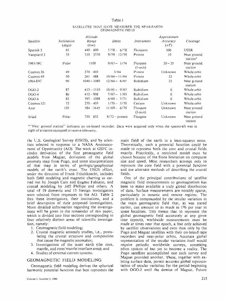
Table I

SATELLITES THAT HAVE MEASURED THE NEAR-EARTH GEOMAGNETI C FI ELD

Altitude Approximate Satellite Inclination Range Dates Instrument Accuracy Coverage

(degs) (km) (nT)

Sputnik 3 65 440-600 5/ 58 - 6/ 58 Fluxgates 100 USSR

Vanguard 3 33 510-3750 9/ 59 - 12/59 Proton 10 Near ground station·

1963-38C Polar 1100 9/ 63 - 1174 Fluxgate 30 - 35 Near ground (I-axis) station

Cosmos 26 49 270 - 403 3/ 64 Proton Unknown Whole orbit

Cosmos 49 50 261 - 488 10/ 64 - 11 / 64 Proton 22 Whole orbit

1964-83C 90 1040 - 1089 12/64- 6/ 65 Rubidium 22 Near ground station

OGO-2 87 413 -1510 10/ 65 - 9/ 67 Rubidium 6 Whole orbit

OGO-4 86 412 - 908 7/ 67 - 1/69 Rubidium 6 Whole orbit

OGO-6 82 397 - 1098 6/ 69 - 717 1 Rubidium 6 Whole orbit

Cosmos 321 72 270 -403 1170- 3170 Cesium Unknown Whole orbit

A zur 103 384 - 3145 11 / 69 - 6/ 70 Fluxgate Unknown Near ground (2-axis) station

Triad Polar 750- 832 9/ 72 - present Fluxgate Unknown Near ground

. " Near ground station" indicates no on-board recorder. sight of a station equipped to receive telemetry.

the U.S. Geological Survey (USGS), and by scien­tists selected in response to a NASA Announce­ment of Opportunity (AO) . The work at GSFC in­cludes derivation of the first geomagnetic field models from Magsat, derivation of the global anomaly map from Pogo, and some interpretations of that map in terms of geologic/geophysical models of the earth's crust. The USGS effort, under the direction of Frank Frischknecht, includes both field modeling and magnetic charting as car­ried out by Joseph Cain and Eugene Fabiano, and crustal modeling by Jeff Phillips and others. A total of 19 domestic and 13 foreign investigators were selected from responses to the AO. Table 2 lists these investigators, their institutions, and a brief description of their proposed investigations . More detailed information regarding the investiga­tions will be given in the remainder of this paper, which is divided into four sections corresponding to four relatively distinct areas of scientific investiga­tion, namely:

I. Geomagnetic field modeling; 2. Crustal magnetic anomaly studies, i.e., postu­

lating the crustal structure and composition that cause the magnetic anomalies;

3. Investigations of the inner earth (the core, mantle, and core/ mantle interface area); and

4. Studies of external current systems.

GEOMAGNETIC FIELD MODELING Geomagnetic field modeling derives the spherical

harmonic potential function that best represents the

Volume I, Number 3,1980

station

Data were acquired only when the spacecraft was in

main field of the earth in a least-squares sense. Theoretically, such a potential function could be made to represent both the core and crustal fields exactly. Practically, a restricted model must be chosen because of the finite limitation on computer size and speed. Most researchers attempt only to represent the core field with a potential function and use alternate methods of describing the crustal fields.

One of the principal contributions of satellite magnetic field measurements to geomagnetism has been to make available a truly global distribution of data. Surface measurements are notably sparse, particularly in oceanic and remote regions. The problem is compounded by the secular variation in the main geomagnetic field that, as was stated earlier, can amount to as much as 1070 per year in some localities. This means that to represent the global geomagnetic field accurately at any given time (epoch), worldwide measurements must be made at times near that epoch, a feat only achieved by satellite observations and even then only by the Pogo and Magsat satellites with their on-board tape recorders and near-polar orbits. Accurate global representation of the secular variation itself would require periodic worldwide surveys, something often spoken of but yet to become a reality. The Pogo satellites accomplished one such survey and Magsat provided another. These, together with ex­isting surface data, permit accurate global represen­tation of secular variation for the period beginning with OGO-2 until the demise of Magsat. Future

215

Investigator

David R. Barraclough

Charles R. Bentley

Edward R. Benton

B. N. Bhargava

Robert F. Brammer

J. Ronald Burrows

Robert S. Carmichael

Richard L. Coles

James C. Dooley

Naoshi Fukushima

Paolo Gasparini

Bruce P . Gibbs

M. R. Godivier

Stephen E. Haggerty

216

Table 2

LIST OF MAGSAT INVESTIGATORS

Institution/Country Title Objectives

Institute of Geological Sciences, United King­dom

Spherical Harmonic Represen- Produce an accurate model of the main geomagnetic field, to­tation of the Main Geomag- gether with reliable estimates of the accuracy of coefficients netic Field for World Charting and Investigation of Some Fundamental Problems of Physics and Geophysics

University of Wisconsin Investigation of Antarctic Using Magsat data, devise a general framework for the struc­Crust and Upper Mantle Using ture of Antarctica into which more specific and local measure­Magsat and Other Geophysical ments can be integrated Data

University of Colorado Geomagnetic Field Forecasting Adjust the gauss coefficients of the main field model of the and Fluid Dynamics of the Magsat data set to satisfy dynamic constraints; use Magsat Core data to test the ability to forecast the structure of the internal

Indian Institute for Geo- Magsat for Geomagnetic Stud-magnetism ies in the Indian Region

geomagnetic field

Prepare a regional geomagnetic reference field and magnetic anomaly maps over Indian and neighboring regions: (a) to gain a clearer understanding of secondary effect features and the variability of the dawn/dusk field, and (b) to study in detail the equatorial electrojet and transient variations

The Analytic Sciences Satellite Magnetic and Gravity Produce magnetic anomaly maps of the Indian Ocean; quantify Corporation (TASC) Investigation of the Eastern the comparison between Magsat data and Geos-3 gravity data;

Indian Ocean interpret the magnetic data using ancillary data

National Research Coun- Studies of High-Latitude Cur- Understand the physical processes that control high-latitude cil of Canada rent Systems Using Magsat current systems; improve the confidence level in studies of in-

Vector Data ternal field sources

University of Iowa Use of Magsat Anomaly Data for Crustal Structure and Min­eral Resources in the U. S. Midcontinent

Energy, Mines and Re- The Reduction, Verification sources, Canada and Interpretation of Magsat

Magnetic Data over Canada

Bureau of Mineral Magsat Data, the Regional Resources, Australia Magnetic Field, and the

Crustal Structure of Australia and Antarctica

Geophysics Research Proposal from Japanese Laboratory, Japan National Team for Magsat

Project

Analyze Magsat anomaly data to synthesize a total geologic model and interpret crustal geology in the midcontinent region; contribute to the interpretation and calculation of the depth of the Curie isotherm

Select quiet-time data; correct Magsat data for disturbance fields and apply the routines; compare Magsat and vector air­borne data; combine Magsat and aircraft data of magnetic anomalies; produce regional interpretations relating to earth structure

Incorporate Magsat data into regional magnetic field charts to improve their accuracy; determine if differences exist in temperature-depth curves for different tectonic areas; study the boundaries between major tectonic blocks and between con­tinental and oceanic crust; determine Curie point depth and crustal magnetization for Antarctica

Analyze the regional geomagnetic field around Japan and Japanese Antarctica; study the contributions to magnetic varia­tions by electric currents and hydromagnetic waves in and above the ionosphere

Osservatorio Vesuviano, Crustal Structures under the Calculate the depth of the Curie temperature for the Italy Active Volcanic Areas of Cen- Mediterranean area and relate to areas of volcanic activity; in­

tral and Eastern Mediterra- vestigate the Italian and Tyrrhenian anomaly nean

Business and Technolog- Geomagnetic Field Modeling Produce a state vector to predict field values for several years ical Systems, Incorpo- by Optimal Recursive Filtering beyond the Magsat model; obtain optimal estimates of field rated values throughout the 1900-1980 period

Office de la Recherche Magnetic Anomaly of Bangui Scientifique et Tech-nique, Outremer (ORSTOM), France

University of Massachu- The Mineralogy of Global setts Magnetic Anomalies

Improve the explanation of the cause of the Bangui anomaly, using Magsat data, other magnetic data, and gravity, seismic, and heat flow data

Interpret Magsat data to locate mafic and ultramafic source rocks and lineament expressions of anomalies that can be cor­related with crustal of upper mantle depths; determine mineral stabilities pertinent to magnetic anomalies to ascertain the magnetic properties of metamorphic rocks

Johns Hopkins APL Technical Digesl

Investigator

D. H. Hall

Christopher G. A. Harrison

David A. Hastings

JohnF. Hermance

William J. Hinze

B. David Johnson

G. R. Keller

David M. Klumpar

John L. LaBrecque

J ean-Louis LeMouel ·

Michael A. Mayhew

Michael A. Mayhew

Igor I. Gil Pacca

Volume I. Number 3.1980

Table 2 (continued)

LIST OF MAGSA T INVESTIGATORS

Institution/Country Title Objectives

University of Manitoba, Identification of the Magnetic Confirm and extend the model for crust mantle magnetization Canada Signatures of Lithostrato­

graphic and Structural Elements in the Canadian Shield Using Magnetic Anomalies and Data from In­dividual Tracks from Magsat

University of Miami

u.S. Geological Survey, EROS Data Center

Brown University

Purdue University

Investigations of Medium Determine the relationship of magnetic anomalies with surface Wavelength Magnetic Anomal- geological features ies in the Eastern Pacific Us-ing Magsat Data

An Investigation of Magsat Determine the Magsat magnetic signatures of various tectonic and Complementary Data Em- provinces; determine the geological associations of these phasizing Precambrian Shields signatures; synthesize Magsat and other data with mineral and Adjacent Areas of West resources data globally Africa and South America

Electromagnetic Deep-Probing Evaluate the applicability of electromagnetic deep-sounding ex­(100-1000 km) of the Earth's perimems using natural sources in the magnetosphere Interior from Artificial Satel-lites; Constraints on the Re-gional Emplacement of Crus-tal Resources

Application of Magsat to Use magnetic anomalies to develop lithospheric models to Lithospheric Modeling in determine the properties of principal tectonic features; correlate South America: Part 1- magnetic anomalies of South America with those of adjacent Processing and Interpretation continental areas to attempt to reconstruct Gondwanaland (see of Magnetic and Gravity Keller below) Anomaly Data

Macquarie Australia

University, An Investigation of the Produce a map of surface magnetization to understand the Crustal Properties of Australia evolution of the crust and to aid in mineral exploration

The University of Texas at EI Paso

The University of Texas at Dallas

Lamont-Doherty Geological Observatory

and Surrounding Regions Derived from Interpretation of Magsat Anomaly Field Data

Application of Magsat to Provide models of the seismic velocity structure of the Lithospheric Modeling in lithosphere (see Hinze above) South America: Part 11- Syn-thesis of Geologic and Seismic Data for Development of In-tegrated Crustal Models

Investigation of the Effects of External Current Systems on the Magsat Data Utilizing Grid Cell Modeling Tech­niques

Analysis of Intermediate­Wavelength Magnetic Anom­alies over the Oceans in Magsat and Sea Surface Data

Apply a modeling procedure to the vector Magsat data in order to separate the terrestrial component from that due to extrater­restrial sources

Determine the distribution of intermediate wavelength magnetic anomalies of lithospheric origin in the oceans, the extent to which Magsat describes the distribution, and the cause of these anomalies

Institut de Physique du Magsat Investigations Consor- Reduce Magsat vector data for a global analytic field model and constant altitude field maps; compare Magsat data to regional studies; study features of the core field; correlate globally and regionally Magsat and gravimetric data

Globe de Paris, France tium

Business and Technolog- Magsat Anomaly Field Inver- Construct a regional crustal temperature/heat flow model ical Systems, Incor- sion and Interpretation for the based on a developed magnetization model, heat flow/ produc-porated U.S. tion data, and spectral estimates of the Curie depth

Business and Technolog- Equivalent Source Modeling Model the core field; compute equivalent spherical harmonic ical Systems, Incor- of the Main Field Using coefficients for comparison with other field models; examine porated Magsat Data the spectral content of the core field

Instituto Astronomico e Geofisico-UPS, Brazil

Structure, Composition, and Construct preliminary crustal models in the Brazilian territory; Thermal State of the Crust in point out possible variations in crustal structure among dif-Brazil ferent geological provinces

217

Table 2 (continued)

LIST OF MAGSA T INVESTIGATORS

Investigator Institution /Country Title Objectives

Thomas A. POlemra The Johns Hopkins University Applied Physics Laboratory

A Proposal for the I nvestiga­tion of Magsat and Tri ad Magnetometer Data to Pro­vide Corrective Information on High-Latitude External Fields

Identify and evaluate high-latitude external fields from the comparison of data acquired by the Magsat and Triad spacecraft that can be used to improve geomagnetic field models

Robert D. Regan Phoenix Corporation Impro ve d Defin i tion of Develop an improved method for the identification of magnetic Cr ustal Magnetic Anomalies anomalies of crustal origin in satellite data by defining better in Magsat Data and removing the most persistent external field effects

Dav id P . Stern NASA/ Goddard Space Study of Enhanced Errors and Estimate the secular variation over the period 1965-80 by Flight Center of the Secular Magnetic Varia- removing mathematical instability based upon scalar field in­

ti on Using Magsa t Models and tensity alone Those Derived in P ogo Surveys

David W. Strangway University of Toronto, Proposal to Analyze the Examine the expected difference between the Grenville and Canada Magnetic Anomaly Maps from Superior provinces

Magsat over Portions of the Canadian and Other Shields

lhn Jae Won North Carolina State Compatibility Study of the Eva luate the compatibility between the Magsat and University Magsat Data and Aeromagnet- aeromagnetic data in the eastern North Ca rolina Piedmont

ic Data in the Eastern Pied-mont of the U.S.

satellite surveys will be needed for accurate global representations beyond the lifetime of Magsat.

Although Pogo data were global and taken over a short time span, the limitation of measuring only the field magnitude resulted in some ambiguity in the field direction in spherical harmonic analyses based on Pogo data alone.3

-6 This ambiguity is be­

ing removed by the acquisition of global vector data with Magsat.

The USGS is currently in the process of updating world and national magnetic charts and field models. Three sets of charts are being prepared: a U.S. chart of declination, a U.S. chart of total field intensity, and a set of world charts for all components. The declination chart was finalized in early 1980, the total intensity charts will be by the end of 1980, and the world charts by August 1981. Magsat data will contribute to all of these charts.

To provide timely input for all applications, a series of field models will be derived from data during magnetically quiet times over the period of data accumulation. One model has already been generated from two full days of data. 7 At ap­propriate intervals it will be updated with addi­tional data, culminating in a final model incor­porating all data with fine attitude coordinate ac­curacy, to be available about October 1981. Magsat data will also be combined with data from the Pogo satellites and other sources to derive predic­tive models with temporal terms.

Of the Magsat data currently available for analy­sis, November 5 and 6, 1979, showed the lowest value of magnetic activity indices. Plots of the data indicated that those days were indeed very quiet magnetically. Accordingly, a selection of 15,206 data points from those days was used to derive the

218

first geomagnetic field model from Magsat, desig­nated MGST (6/80). 7 The spherical harmonic coef­ficients are given in Table 3. Vector data above 50° latitude were not included because of non-curl-free fields from field-aligned currents. Such fields are transverse to the main field and, as shown by Langel,2 have little or no effect on the field magnitude. However, 3354 values of B" 3345 of Bo, and 3361 of B<I> were included for latitudes below 50°. (B" Be, and B<I> are the radial, north­south, and east-west components - in a spherical coordinate system - of the geomagnetic field.)

This model fits the selected data with the mean and standard deviations as follows:

Mean Standard Component Deviation Deviation

(nT) (nT) Scalar mag-

nitude 0.1 8.2 B, 2.5 6.5 Be -0.1 7.6 B<I> 0.5 7.4

The deviations are mainly due to a combination of fields from unmodeled external and crustal sources.

As part of our preparation for Magsat, Pogo data were combined with surface data from obser­vatories between 1960 and 1977, with selected repeat data, and with selected shipborne data to derive what we consider to be the best possible pre­Magsat model. 8 Constant and first-, second-, and third-derivative time terms were included to degree and order 13, 13, 6, and 4, respectively. This model, designated PMAG (7/80), used a new tech­nique for dealing with the observatory data. As at

Johns H opkins APL Technical Digest

Table 3

SPHERICAL HARMONIC COEFFICIENTS FOR MAGSAT GEOMAGNETIC FIELD MODEL MGST (6/80)

Internal Coefficients (nn

n m gn m h n m n m gflm h n m

0 - 29989.6 9 8 1.4 -5.9 1 1 - 1958.6 5608.1 9 9 -5. 1 2.1 2 0 - 1994.8 10 0 - 3.3 2 1 3027.2 -2127.3 10 1 -3.5 1.4 2 2 1661.6 - 196.1 10 2 2.5 0.4 3 0 1279.9 10 3 -5.3 2.6 3 I - 2179.8 - 334.4 10 4 -2.1 5.6 3 2 1251.4 270.7 10 5 4.6 - 4.2 3 3 833 .0 -251 .1 10 6 3.1 - 0.4 4 0 939.3 10 7 0.6 - 1.3 4 I 782 .5 211.6 10 8 1.8 3.5 4 2 398.4 -256.7 10 9 2.8 -0.5 4 3 -419.2 52.0 10 10 - 0.5 -6.2 4 4 199.3 - 297.6 II 0 2.4 5 0 - 217.4 II I - 1.3 0.7 5 1 357.6 45.2 II 2 -1.9 1.7 5 2 261.0 149.4 11 3 2.2 -1.1 5 3 -73.9 - 150.3 II 4 0.1 - 2.7 5 4 - 162.0 -78. 1 II 5 -0.4 0.6 5 5 -48.3 91.8 II 6 - 0.3 - 0.1 6 0 48 .3 II 7 1.7 -2.4 6 I 65 .2 -14.5 II 8 1.8 - 0.3 6 2 41.4 93.4 11 9 - 0.6 -1.4 6 3 - 192.2 70.6 II 10 2.1 -1.6 6 4 3.5 - 42.9 II II 3.5 0.6 6 5 13 .7 -2.4 12 0 - 1.6 6 6 - 107.6 16.9 12 1 0.4 0.6 7 0 71.7 12 2 - 0.1 0.6 7 I - 59.0 -82.4 12 3 - 0.1 2.3 7 2 1.6 - 27.5 12 4 0.6 -1.5 7 3 20.5 -4.9 12 5 0.5 0.5 7 4 - 12.6 16.1 12 6 -0.6 0.2 7 5 0.6 18. 1 12 7 - 0.4 -0.4 7 6 10.6 -22.9 12 8 0.1 0.0 7 7 - 2.0 - 9.9 12 9 -0.4 0.0 8 0 18.4 12 10 -0.2 - 1.5 8 I 6.8 6.9 12 II 0.7 0.3 8 2 -0.1 - 17 .9 12 12 0.0 0.7 8 3 -10.8 4.0 13 0 0.0 8 4 - 7.0 -22.3 13 I -0.5 - 0.4 8 5 4.3 9.2 13 2 0.3 0.4 8 6 2.7 16 .1 13 3 - 0.7 1.6 8 7 6.3 - 13.1 13 4 0.0 0.0 8 8 - 1.2 -14.8 13 5 1.2 - 0.6 9 0 5.6 13 6 - 0.4 -0. 1 9 I 10.4 - 21.1 13 7 0.4 0.8 9 2 1.1 15.2 13 8 -0.6 0.2 9 3 - 12.6 8.9 13 9 0.2 0.8 9 4 9.5 - 4.8 13 10 0.1 0.5 9 5 -3.3 -6.5 13 11 0.4 - 0.1 9 6 - 1.3 9.0 13 12 -0.4 0.0 9 7 6.8 9.5 13 13 0.0 - 0.1

External Coefficients (nn

n m gnl1l /1,,11/

0 20.4 -0.6 - 0.4

The mean radius of the earth is 6371.2 km The mean epoch is 1979.85

Volume I, Number 3,1980 219

the satellite, surface fields contain contributions from the three sources. For field modeling the an­nual mean value for each observatory is usually used so that the external contribution is some averaged value (we hope, small). However, crustal anomaly fields are typically quite large. For past models the rms residual of surface data to the model has been typically between 100 and 200 nT. 9

We have incorporated a procedure for solving in­dependently for the "bias" or anomaly field in each component at each observatory. This pro­cedure was used for the first time in the derivation of the PMAG (7 / 80) model. After solving for the coefficients of the potential function and the obser­vatory biases, the rms residual of the observatory data was reduced to below 28 nT for all com­ponents. For repeat data this procedure was not feasible because of a lack of extensive temporal coverage. These data were incorporated by in­cluding only locations where three or more measurements, made at different times, were available. Each component at each location was then represented by a linear fit; only the rate of change was used in deriving PMAG (7 / 80) . The residual to the fit was 10 nT per year for all com­ponents. For shipborne data, 39 long tracks in regions devoid of other surface measurements were selected. These were low-pass filtered with a cutoff of 500 km to eliminate the crustal anomaly field . The rms residual to the fit was 38 nT. Extension of this model by the addition of Magsat data does not change the above quoted residuals a great deal, and the resulting model, GSFC (9/ 80), is in good agree­ment with MGST (6/ 80) at the Magsat epoch.

Using quick-look data from the first few days of Magsat operation, various pre-Magsat models were evaluated. These results are summarized in Table 4.

Global geomagnetic models will be undertaken by the USGS (Cain, Fabiano) and by the French

investigators under the direction of LeMouel and the British investigators under the direction of Bar­raclough. The USGS investigators, in addition to publishing charts of the field, will pay particular attention to the problem of separating the core, crustal, and external contributions to the field, and of developing an adequate mathematical represen­tation of each. The French and British will attempt a very accurate model of secular variation for pre­dicting the field in the future and for studying pro­perties of core fluid motions and interactions at the core/mantle boundaries. In addition to the global models, several investigators will attempt more ac­curate regional models for particular areas in order to isolate better the crustal anomaly fields in those areas.

Magsat will provide an accurate model of the main geomagnetic field, but its lifetime was too short for determining the secular variation of the field. The secular variation can be determined through comparison with earlier global surveys of the geomagnetic field from space, but such surveys are known to suffer from enhanced errors in cer­tain sequences of harmonic terms. Stern (GSFC) will use the Magsat model to evaluate the extent ~f such enhanced errors, correct them, and then use the corrected models for deriving the mean secular variation over the 1965-1980 period.

Gibbs (Business and Technological Systems) will attack the secular variation problems from a sta­tistical point of view by using recursive estimation theory to combine conventional models into op­timal estimates of the field parameters for any given time. The statistical information so derived should enable a more accurate prediction capability as well as more accurate a posteriori models.

An alternative to the classical spherical harmonic representation will be attempted by Mayhew (Business and Technological Systems). He will

Table 4

RESIDUALS OF SELECTED MAGSA T DATA TO SOME PUBLISHED FIELD MODELS (nT)

POGO (2 /72)10 IGRF 1975 11 A WC/75 12 IGS/75 13 WC80 14 PMAG(7/ 80) H

Scalar: mean deviation 9 -91 60 21 -21 -2 standard deviation 105 124 125 119 117 79 rms deviation 105 154 139 121 119 82

Br : mean deviation 6 12 25 20 31 13 standard deviation 208 192 152 134 121 93 rms deviation 208 192 154 135 125 94

Be: mean deviation 18 51 -4 15 22 33 standard deviation 114 108 93 84 89 59 rms deviation 115 120 94 86 92 67

B .. : mean deviation 0 2 0 I standard deviation 165 125 89 89 61 61 rms deviation 165 125 89 89 61 61

220 Johns Hopkins APL Technical Digest

adopt methods of anomaly modeling by equivalent sources, representing the main field with an array of dipoles at a fixed radius within the core. If such a method proves feasible, it will potentially use less computer time than the usual methods.

CRUSTAL MAGNETIC ANOMALY INVESTIGA TIONS

A crustal magnetic anomaly is the residual field after estimates of the core and external fields have been subtracted from the measured field. An anomaly map is a contour map of the measured average anomaly field at the altitude of the data. Anomaly maps have been derived from aeromag­netic and shipborne data for many years and used in the construction of geologic/ geophysical models of the crust. Investigations with aeromagnetic and shipborne magnetic data have mainly concentrated on the very localized anomalies associated with small-scale geologic features and localized minerali­zation. However, in the past few years there has been an increased interest in studies of the broad­scale anomalies that appear in regional compila­tions of aeromagnetic and shipborne data. 15

-19

Satellite anomaly maps are of recent origin and describe only the very broadest scale anomalies. Aeromagnetic and ship borne anomaly maps have usually been interpreted assuming a flat earth and a constant ambient field over the region of interest. Because of the extremely large scale of satellite­derived anomalies, both of these assumptions

become invalid, thus necessitating development of new analysis techniques .

Originally, it was thought impossible to detect fields of crustal origin in satellite data. However, while analyzing data from the Pogo satellites, Regan et al. 20 discovered that the lower altitude data contained separable fields caused by crustal anomalies, thus opening the door to a new class of investigations. None of the satellites shown in Table 1 was designed for solid earth studies , yet results from the Pogo satellites have demonstrated the capability of mapping broad-scale anomalies. Although the map of Regan et al. was partially contaminated by "noise" from magnetospheric and ionospheric fields, the reality and crustal origin of several of the anomalies defined by the map were clearly demonstrated. More recently Langel et al. 10

have compared a Pogo-derived anomaly map with upward-continued aeromagnetic data from western Canada. Figure 1 shows the results of that com­parison. The two maps are in substantial agree­ment, demonstrating further both the reality and crustal origin of the anomalies.

The techniques for preparing such a map include selecting suitable quiet-time data, removing the best estimate of the fields not originating in the earth 's crust, and averaging data at the appropriate resolu­tion. It is believed that these techniques can be readily adapted to Magsat data, both scalar and vector. It will be some months before an anomaly map is available from Magsat data . Individual pass residuals, however, clearly show the presence of

Fig. 1-Comparison of anomaly maps from upward continued aeromagnetic data and from Pogo data. Units are nanoteslas (nT).

Volume 1, Number 3,1980 221

these crustal fields. Figure 2, for example, shows the Bangui or Central African anomaly first dis­covered by Regan et al. 20

The basic anomaly maps are only a starting point for interpretation. To maximize their usefulness they must be transformed to a common altitude and to the anomalies that would be present if the earth's field had the same inclination everywhere (reduction to a common inclination) . Preliminary techniques for reduction to common altitude now exist and have been applied to Pogo data between ± 50° latitude. The resulting map is shown in Fig. 3.

For geologic studies such anomaly maps must be inverted to a description of the magnetic properties of the crustal rocks. The inversions are not unique; constraints from other data sources will be required in their interpretation. As a first step in such modeling: traditional equivalent source methods, adapted for the case of a spherical earth with changing field inclination, have been applied to the United States 21 and Australia.22 This technique assumes a constant 40 km thickness of the magnet-

aJ <l

25,-----------------,------------------,

I \ \ '\

-25~--------------~~----------------~

30° 0° Latitude

Fig. 2-The Bangui or Central African anomaly as seen in Magsat data. The equatorial longitude is 14.6'; the altitude is 425 km . .lB is the residual anomalous field after subtracting a model of the core field from the measured field.

50

., 120 160 40

ic crust and derives the magnetization in such a crust that would cause the anomalies seen at the spacecraft. All of the anomalous field is assumed to be induced; i.e., remanent magnetization is assumed to be zero. The results for the United States are shown in Fig. 4. In many regions, known geologic features are clearly outlined (e.g., the Basin and Range Province, Colorado Plateau, Rio Grande Rift, Michigan Basin, and Mississippi Em­bayment) whereas some features are notable by the absence of magnetic features (e.g ., the mid­continent gravity high). It will be some years before these maps are fully understood and interpreted, but they promise to shed new light on the geology of the deep crust.

Anomaly maps, or even magnetization maps, are not an end in themselves. The object of these ef­forts is to derive models of the crust and upper mantle for large-scale regions of the globe. There are many kinds of models; their common purpose is to generalize observations and prediction . Through synthesis of particular models, complex models of crustal geologic systems are built up in terms of structural and compositional variations and the movements of material and energy. Con­clusions can then be drawn about the evolution of regions that lead to inferences about the distribu­tion of natural resources.

Figure 5 is an outline of an example of how one might think of the process of synthesizing models, beginning with satellite magnetic field data and in­cluding correlation with other data types. Models of gross variations in mean magnetization to the Curie isotherm can be developed from satellite data. This serves to quantify the anomaly map and can be of great utility in more detailed analysis of the data. Correlatively, from gravity measurements, variations in mean density to some fixed depth can be inferred, assuming homogeneity below that depth. These models can be combined with velocity

• 200

280 320 -'- - -

Na noteslas -8 to - 10 - 6 to -8 -4 to -6 - 2 to - 4 2 to 4 4 to 6 6 to 8

360 8 to 10 _ _ _ CJ C:=

C] --Fig. 3-Scalar magnetic anomaly map from the Pogo satellites reduced to 500 km altitude.

222 Volume I, Number 3,1980

Fig. 4-Equivalent bulk magnetization derived from Pogo satellite data assuming a constant·thickness magnetic crust of 40 km. Units are EMU/cm3 x 104 •

models based on seismic data and with composi­tional models based on laboratory measurements of rock properties to give large-scale models of crustal structure and composition. Similarly, models of rel­ative movements and of temperature distribution can be built for very large regions . These large­scale models can then be used to make more de­tailed models for smaller regions using a variety of data, some of which are also listed in Fig. 5. There are no hard and fast rules about the combination sequence, which depends on the region and the data available. Further, the process is an iterative one in which new data are sought based on predic­tions from interim models.

Data (examples)

The Pogo satellites from which these maps were derived had two severe limitations for the studies: the altitude range was high (most data were from above 500 km), and the data were of field magni­tude only . Magsat addresses both shortcomings . Its lower altitude increases the resolution by roughly a factor of 2 and the field strength of the anomalies by a factor of between 2 and 5, depending on the geometry of the source region. This is dramatically illustrated in Fig. 6, which shows a comparison be­tween the lowest altitude Magsat data and low­altitude Pogo data. The Magsat data are at 187-191 km, while the Pogo data are at 414-420 km. The tracks are nearly coincident geographically.

Lithospheric Models

Satellite

Magnetics

Gravity

Overall regional model

Imagery (regional)

Correlative

Seismic

Heat flow

Field geology

Comparative planetology

Satellite

Imagery (visual / I R/therm Altimetry Radar Passive microwave

Correlative Aeromagnetic Surface gravity Detailed seismology M agnetote II uric Petrologic/ radiometric Tilt, vertical movement Mineralization distributio

Volume I, Number 3,1980

all

n

Relative magnetization/curie isotherm depth

Density

Stru ctu ref to pograp hy / mega linea me nts

Regional velocity structure

Regional heat flux

Geologic/ tectonic maps

Evol utionary models

Refined composite mode l for selected subregions

~

Tectonic history Resource assessment, Hazard assessment

Fig. 5-Synthesis of geolog· ic/geophysical models (ideal­ized out line).

223

Anomaly map at 500 km derived from Pogo data

DD •• -4 to - 6 - 2 to -4 2 to 4 4 to 6

(nT)

140 160 180 Longitude (deg)

2.0 Magsat data ; June 10, 1980

~I titude: 187-191 km

~ - 14.0 '0 r''''"'--- - _ a; _30.0L----"'--_'-----" _ ___1 _ ___1-=.___1 _ ___1_--' _ ___'

:;:

~ 9.0 '0 .;;;

~ -3.0

Pogo-4 data ; December 17, 1967 Altitude: 414-420 km

-15,0 '-----"~'--'--___1 _ ___1 _ ___1 _ ___1 _ ___1_--' _ ___'

34.9 32.1 29.3 26.5 23.7 20.9 18.1 15.3 12,5 9.7 Latitude (deg)

Fig. 6-Comparison between Pogo (OGO·4) data and the lowest altitude data from Magsat.

Magsat's lower altitude greatly enhances the resolu­tion and signal strength of the anomalies. With field magnitude data, only indirect estimates of remanent magnetization are possible. 23 The vector data from Magsat measure anomaly directions other than along the earth's main field.

GSFC will derive a basic global magnetic anoma­ly map from the Magsat data. Many investigators will use that map or the associated magnetization map directly in their investigations. Other investiga­tors will reexamine the basic derivation of the anomaly map and seek to extend or modify these techniques. Among the latter are:

Investigator

Bhargava Fukushima Coles and Hall Hinze and Keller Mayhew

224

Region Investigated

India Japan and vicinity Canada South and Central America United States

Johnson and Dooley

LeMouel Australia and Antarctica Europe and Central Africa

This type of modeling will be used by the in­vestigators just listed for the continent-size regions indicated . When the larger region has been model­ed, features of particular interest will become the subject of more intensive investigations. In some cases existing tectonic features have already been singled out for more localized modeling, such as the Narmada-son lineament in central India (Bhargava), the Superior province of Canada (Strangway), or the Japan Trench (Fukushima).

Continental-scale studies will utilize maps made at GSFC, including those of Pacca (Brazil), Bentley (Antarctica), and Hastings (Africa and South America) .

Mayhew, Hinze, Coles, and Pacca will pay par­ticular attention to mapping the Curie isotherm. Hinze, Keller, and Hastings are interested in the implications of the Magsat data for the plate­tectonic reconstruction of Africa and South Ameri­ca, a topic now under study by Langel, Frey, and Mead at GSFC using the Pogo data.

In addition to the continental-scale studies, several investigators will study more limited areas or particular tectonic features. Godivier (ORSTOM) will extend the work of Regan and Marsh24 in the region around the Central African Republic where ORSTOM has a large amount of correlative data. Gasparini (Osservatorio Vesu­viano) will investigate the Curie depth and volcanism in the Mediterranean area. Won (North Carolina State University) will study a combination of Magsat, aeromagnetic, and regional gravity data in the eastern Piedmont of the United States. Car­michael and associates (University of Iowa) will study the central midcontinent of the United States with particular attention to the known midconti­nent geophysical anomaly.

In contrast to the large number of investigators studying continental-type regions, only three in­vestigators are giving concentrated attention to oceanic regions. There are several reasons for this. First, the satellite anomaly maps derived from Pogo data show very few anomalies in oceanic regions compared to continental regions. Second, theoretically, the thinner oceanic crust should not contain anomalous features of comparable size to continental crust. Harrison (University of Miami) notes that a minimum in the power spectrum should occur between the contributions from core and crustal sources but that such a minimum is not present in spectra from shipborne data over oceanic basins. He will use Magsat data to study the inter­mediate wavelength anomalies. Brammer (T ASC) will concentrate his efforts on a study of Magsat and Geos-3 altimeter gravity data in the eastern In­dian Ocean.

LaBreque (Lamont-Doherty) will organize the ex-

johns Hopkins APL Technical Digesl

isting shipborne data in an effort to help describe the secular variation over oceanic areas and to pro­vide surface anomaly maps suitable for upward continuation and comparison with Magsat data .

Underlying all crustal models derived from Magsat and correlative data is a need for understanding the basic magnetic properties of crustal rocks. Such understanding depends on careful laboratory measurements, some at the higher temperatures and pressures of the lower crust. Preliminary studies 25 have already claimed to show the extremely significant result that the Moho is a magnetic boundary even when the Curie iso­therm lies in the mantle. Wasilewski and the other GSFC investigators are continuing these efforts. Particular attention to petrologic constraints, the effects of oxygen fugacity, and other properties will be given by Haggerty (University of Massachu­setts). A substantial refinement of the petrology of source rocks responsible for deep crustal anomalies is expected.

INVESTIGATIONS OF THE INNER EARTH

Man has directly penetrated only a few kilometers of the 6371 km distance to the earth's center. Information about the inner earth must be obtained by indirect methods such as seismology and measurements of the gravitational and mag­netic fields.

Combining Magsat data with Pogo and near­surface surveys will permit more accurate deter­mination of the secular variation of the core field. This variation will be used by Benton (University of Colorado) to study properties of the fluid mo­tions in that core; in turn, appropriate magnetohy­drodynamic constraints will be investigated to determine if they can aid in better modeling the secular variation.

When they are time-varying, magnetospheric

Volume I, Number 3, 1980

fields result in induced fields within the earth because of the finite conductivity of the earth. The characteristics of these induced fields are deter­mined by the properties of the materials in the earth's mantle (i.e., composition, temperature). At present the limiting factor in determining a precise conductivity profile within the earth, with adequate spatial resolution, is the accuracy possible in deter­mining the external and induced fields. Hermance (Brown University) will use Magsat vector measure­ments together with surface data for a more accu­rate analysis than was previously possible.

STUDIES OF EXTERNAL CURRENT SYSTEMS

Early observers of the earth's magnetic field discovered that it continually undergoes transient changes. These changes include systematic varia­tions that occur with daily regularity and irregular variations, both of amplitude and of a totally dif­ferent kind, superimposed on the regular varia­tions . Periods of time when the changes are mostly regular are called magnetically quiet; periods when the magnetic disturbances become irregular are called magnetically disturbed. When the irregular fields are large but mainly confined to high lati­tude, the condition is called a magnetic substorm; when the irregular fields are large and worldwide, it is called a magnetic storm. To understand such changes in field, one must realize that the space surrounding the earth contains several "species" of electric current. The energy for these currents comes ultimately from the sun. Figure 7 is an ar­tist's conception (based on Fig. 1 of Heikkila/6

wherein there is a more detailed explanation) of the magnetic environment of the earth. A stream of charged particles from the sun, called the solar wind, confines the earth's magnetic field to a cavity known as the magnetosphere. This cavity is com­pressed on the front, or sunward, side and drawn

Fig. 7 -Artist's conception of the configuration of the mag­netosphere, adapted from Heikkila. 26 The magneto­sphere is the region into which the earth's magnetic field is confined by the solar wind.

225

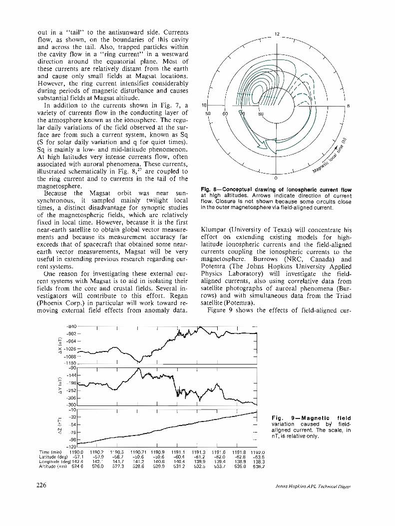
out in a "tail" to the antisunward side. Currents flow, as shown, on the boundaries of this cavity and across the tail. Also, trapped particles within the cavity flow in a "ring current" in a westward direction around the equatorial plane. Most of these currents are relatively distant from the earth and cause only small fields at Magsat locations. However, the ring current intensifies considerably during periods of magnetic disturbance and causes substantial fields at Magsat altitude.

In addition to the currents shown in Fig. 7, a variety of currents flow in the conducting layer of the atmosphere known as the ionosphere. The regu­lar daily variations of the field observed at the sur­face are from such a current system, known as Sq (S for solar daily variation and q for quiet times). Sq is mainly a low- and mid-latitude phenomenon. At high latitudes very intense currents flow, often associated with auroral phenomena. These currents, illustrated schematically in Fig. 8,27 are coupled to the ring current and to currents in the tail of the magnetosphere.

Because the Magsat orbit was near sun­synchronous, it sampled mainly twilight local times, a distinct disadvantage for synoptic studies of the magnetospheric fields, which are relatively fixed in local time. However, because it is the first near-earth satellite to obtain global vector measure­ments and because its measurement accuracy far exceeds that of spacecraft that obtained some near­earth vector measurements, Magsat will be very useful in extending previous research regarding cur­rent systems.

One reason for investigating these external cur­rent systems with Magsat is to aid in isolating their fields from the core and crustal fields. Several in­vestigators will contribute to this effort. Regan (Phoenix Corp.) in particular will work toward re­moving external field effects from anomaly data.

Time (min) 1190.0 1190.2 1190.5 1190.71 1190.9 1191.1 Latitude (deg) -57.1 -57.9 -58.7 -59.6 -59.6 -60.4 Longitude (deg) 142.4 142.1 141 .7 141 .2 140.8 140.4 Altitude (km) 524.6 526.0 527.3 528.6 529.9 531 .2

226

18 f----+--!.J.JIl-1Ll--=-i I--L-':'+--~----l----I 6

o

Fig. a-Conceptual drawing of Ionospheric current flow at high altitudes. Arrows indicate direction of current flow. Closure is not shown because some circuits close in the outer magnetosphere via field·aligned current.

Klumpar (University of Texas) will concentrate his effort on extending existing models for high­latitude ionospheric currents and the field-aligned currents coupling the ionospheric currents to the magnetosphere. Burrows (NRC, Canada) and Potemra (The Johns Hopkins University Applied Physics Laboratory) will investigate the field­aligned currents, also using correlative data from satellite photographs of auroral phenomena (Bur­rows) and with simultaneous data from the Triad satellite (Potemra).

1191.3 -61 .2 139.9 532.5

Figure 9 shows the effects of field-aligned cur-

1191 .6 1191.8 -62.0 -62.8 139.4 138.9 533.7 535.0

1192.0 - 63.6 138.3 536.2

Fig. 9-Magnetic field variation caused by field­al igned current. The scale, in nT, is relative only.

Johns H opkins APL Technical Digesl

rents in Magsat data. b.X, b. Y, b.Z are residuals from a field model in a north-, east-, and down­coordinated system. Large-amplitude, highly st ruc­tured variations occur in the north and east direc­tions but not in the vertical direction, as expected from field-aligned currents.

CONCLUSION Satellite-based magnetic field measurements

make global surveys practical for both field model­ing and for the mapping of large-scale crustal anomalies. They are the only practical method of accurately modeling the global secular variation . Magsat is providing a significant contribution, both because of the timeliness of the survey and because its vector measurement capability represents an ad­vance in the technology of such measurements.

Data from Magsat are available for any inter­ested user through the National Space Sciences Data Center at GSFC.

With the success of Magsat, future missions should take two courses. Field modeling requires periodic surveys, but not low-altitude measure­ments as required for crustal studies. On the other hand, further advances in satellite crustal studies will rest on NASA' s ability to orbit magnetometers at still lower altitudes; such concepts are still in the stage of discussions as to their feasibility.

REFERENCES I J . C. Cai n and R. A. La ngel, " Geomagnetic Survey by the Polar- Or­

biting Geophysica l Obse rvatories," World Magnelic Survey 1957-1969 (A. J. Zmuda, ed.) IAGA Bulleti n No . 28 (197 1) .

2R. A. Langel, "Near Earth Magnetic Dist urbance in Total Field at High Latitude, I. Sum mary of Data from OGO 2, 4, and 6," 1. Geophys. Res. 79, pp . 2363 - 237 1 (1974) .

3G. E. Backus, "Nonuniqueness of the External Geomagnetic Field Determined by Surface Intensity Measurements," 1. Geophys. Res. 75 , pp. 6339 - 634 1 (1970).

4L. Hurwitz and D. G. Knapp , " Inherent Vector Discrepancies in Geomagnetic Main Field Models Based on Scalar F," 1. Geophys. Res. 74 , pp. 3009-3013 (1974).

5D. P. Stern and J. H . Bredekamp, "Error Enhancement in Geomagnetic Models Derived from Scalar Data," 1. Geophys. Res. 80, pp. 1776 - 1782 (1975).

6F. J. Lowes, "Vector Errors in Spherical Harmonic Analys is o f Scalar Data," Geophys. 1. Roy ASlron. Soc. 42, pp. 637 - 651 (1975).

7R. A. Langel, R. H . Estes, G. D. Mead, E. B. Fabiano, and E. R. Lancaster, " Initial Geomagnetic Field Model from Magsal Vector Data," Geophys. Res. Lell. (in press).

SR. A. Langel, R. H . Estes, G. D. Mead, and E. R. Lancaster, "A Model of the Earth's Magnetic Field, 1960 - 1980" (in preparation).

Volume I , Number 3,1980

9J. C. Cain, S. J . H endricks, R. A. Langel, and W. V. Hudson, "A Proposed Model for the Int ernat ional Geomagnetic Reference Fields -1965 ," 1. Geomagll. GeoeleClr. 19, pp. 335 - 355 (1967).

tOR. A. Langel , R. L. Co les, and M. A . Mayhew, "Comparisons of Magnet ic Anoma li es o f Lit hospheric Origin as Measu red by Sa tellite and by Airbo rne Magnetometers over Western Canada, " Call. 1. Earlh Sci. X VII, pp. 876 - 887 (1980).

tt lAGA Di vis ion I Study Group, " Int ernational Geomagnetic Reference Field 1975," EOS, 57, pp. 120 - 121 (1976) .

t2D. R. Barraclough, J. M. Harwood , B. R. Leaton, and S. R. C. Malin , " A Model of the Geomagnetic Field at Epoch 1975" Geophys. 1. R. ASlroll . Soc. , 43 , pp. 645 - 659 (1975) .

l3N. W. Peddie and E. B. Fabia no, "A Model of the Geomagnetic Field for 1975 ," 1. Geophys. Res. 81 , pp. 1539 - 2542(1976).

14F. S. Baker and D. R. Barraclough , " World Magnetic Chart Model for 1980," EOS 61, p. 453 (1980) .

15L. C. Pakiser and l. Zietz, "Transcontinental C rustal and Upper Man­tle St ructure," Rev. Geophys. 3, pp. 505 - 520 (J965).

t6l. Zie tz, E. R. King . W. Geddes, and E. G. Lidiak , "Crustal Stud y of a Continental Strip fro m the Atlantic Ocean to the Rock y Moun­ta ins," Geolog. Soc. Am. BII/I. 77, pp. 1427 - 1448 ( 1966) .

17R. T. Shuey, D. R. Schellinger, E. H . Johnson , and L. G. Alley, "Aeromagnetics and the Transition between the Colorado Plat eau and th e Basin Range Province," Geology 1, pp. 107 - 110 (1973).

18D. H. Hall, "Long-Wavelengt h Aeromagnetic Anomalies and Deep Crustal Magnetization in Manitoba and North Western O ntario, Canada," 1. Geophys. 40, pp. 403 - 430 (1974) .

t9A. A. Kruithovskaya and l. K. Paskevich, " Magnetic Model for the Earth 's Crust under the Ukra inian Shield," Call . 1. Earlh Sci. 14, pp. 27 18 - 2728 (1977).

2o R. D. Regan, J . C. Cain , and W. M. Davis, " A Global Magnetic Anomaly Map," 1. Geophys. Res. 80, pp. 794 - 802 (J975 ).

21M. A. Mayhew, "Satellit e Derived Equivalent Magnetization of the United States" (in preparation, 1979).

22M. A. Mayhew, B. D. Johnson , and R. A . Langel , "Magnetic Anomalies a t Sa telli te Elevat ion over Aust ralia " (submitted to Earlh Plallel. Sci. Lell. , 1980) .

23 B. K. Bhattacharyya, " Reduction and Treatment of Magnetic Anomalies of Crustal Origin in Sa tell ite Data," 1. Geophys. Res. 82 , pp. 3379 - 3390 (1977).

24R. D. Regan and B. D. Marsh, "The Bangui Anomaly: Its Geological Origi n," 1. Geophys. Res. (in press).

25p. J. Wasilewski , H . H. Th omas, and M . A. Mayhew, " The Moho as a Magneti c Boundary," Geophys. Res. Lell . 6, pp. 54 1 - 544 (1979).

26W. J. Heikkila , " Penetrat ion of Particles into the Polar Cap Regions of the Magnetosphere, " Crilical Problems of MagnelUspheric Physics (E. R. Dyer, ed .), IUCSTP Secretariat (1972) .

27R. A . Langel, "Near Earth Magnetic Disturbance in Total Field at High Latitude, 2. Interpre tation of Data from OGO 2. 4, and 6," 1. Geophys. Res. 79 , pp. 2373 - 2392 (1974).

ACKNOWLEDGMENTS - I wish to thank all members of the Magsat team for making possibl e the acquisition and analysis of these data. Although it is not feasible to name all those included, my special thank s go to Gil Ousley of GSFC and L. D. Eckard of APL for directing the ef­fort that cu lminated in the success ful construction, launch, and operation of Magsat; to Mario Acuna and W. H. Farthing for the design and over­sig ht of the magnetometers; to John Berbert and Earl Beard of GSFC and Don Berman of Computer Science Corporation and their colleagues for their efforts at data preparation; and to Locke St uart and hi s team at GSFC for their successful o rganization of and interface with the Magsa t investigators. Finally, I particularly appreciate the encouragemenl, ad­vice, and general support of Gil Mead , Lou Walter, and Barbara Lueders of the GSFC Geophysics Branch.

227

THOMAS A. POTEMRA

STUDIES OF AURORAL FIELD-ALIGNED CURRENTS WITH MAGSAT

Electric currents that flow between the outermost boundaries of the magnetosphere and the auroral zones, sometimes deliver more power to the earth than is generated in the entire United States at any given time. These field-aligned "Birkeland" currents are detected on a regular basis by Magsat.

INTRODUCTION

Following earlier suggestions by Edmund Halley and Anders Celsius that the auroral phenomena behave magnetically, Kristian Birkeland discovered in his polar expeditions of 1902-03 that large-scale currents were associated with the aurora. He was also the first to suggest that these currents originated far from the earth and that they flowed into and away from the polar atmosphere along the geomagnetic field lines. The existence of such field­aligned currents was widely disputed because it was not possible from a study of only surface magnetic field measurements to distinguish unambiguously between current systems that are field aligned) and those that are completely ionospheric. 2 Further­more, theoretical calculations3

,4 predicted that the effects of field-aligned currents may be impossible to detect with ground-based magnetometers for cer­tain models of these current systems.

The first experimental confirmation of the pres­'ence of field-aligned ("Birkeland") currents was provided by A. J. Zmuda and his colleagues5

,6 who studied magnetic disturbances in the polar regions of the earth, observed with the single-axis magne­tometer used in the attitude determination system on the APLlU.S. Navy 5E-I (1963-38C) satellite. That satellite, launched on September 28, 1963, in­to a nearly circular polar orbit at an altitude of 1100 km, carried an array of particle detectors and a fluxgate magnetometer. 7

Zmuda5•6 discovered that disturbances normal to

the main geomagnetic field were often observed with 5E-l in the same region of the earth associ­ated with a variety of auroral phenomena. It was soon realized that the transverse disturbances could be interpreted as being caused by electric currents flowing along the geomagnetic field lines, and thus the first study of the global characteristics of Birkeland currents was begun at APL.

Recognizing the importance of sensitive satellite magnetic field measurements to the study of Birke­land currents, Armstrong and Zmuda8 suggested a

228

modification to the attitude magnetometer system for the APLlU.S. Navy Triad satellite. The Triad satellite was launched into a polar orbit at an altitude of 800 km on September 2, 1972, and, un­til the launch of Magsat on October 30, 1979, was the only satellite making continuous and high­resolution magnetic observations in the polar regions. The Triad magnetometer provides 2.25 vector samples per second with a resolution of 12 nanoteslas (1 nT = 10,9 weber per square meter), made possible by the 13-bit analog-to-digital con­verter incorporated into the system following the suggestion of Armstrong and Zmuda. The Triad magnetic field observations were used to determine for the first time the flow directions, spatial distribution, and intensities of Birkeland currents and their relationships to a variety of geophysical phenomena such as optical emissions, current­driven plasma instabilities, ionospheric currents, geomagnetic storms, and interplanetary phenome­na. During its brief lifetime, the improved Magsat magnetic field observations were correlated with the Triad observations to compile more informa­tion about the important Birkeland currents and to calibrate the Triad magnetometer. Fortunately for these studies, Magsat was launched near the time of the peak solar cycle (the larges t in many II-year cycles) so that disturbances produced by the Birke­land currents were observed on almost every orbit.

The importance of Birkeland currents to the coupling between outer space and the auroral at­mosphere is emphasized by their total intensity, which ranges between 106 and 107 A, and by the energy they dissipate in the upper atmosphere, which can exceed by a considerable factor the energy deposition associated with the dramatic, visual, auroral forms. The Birkeland currents are also the critical ingredient in a variety of com­plicated plasma phenomena that have important applications to earth (associated with substorms and the aurora) , to Jupiter (associated with 10-related radio emissions), ~.)O and to the galaxy (related to comets and double radio sources). ))

johns Hopkins APL Technical DiJ!,esl

MAGNETIC DISTURBANCES AND FIELD-ALIGNED CURRENTS

The magnitude and direction of equivalent cur­rents associated with magnetic disturbances, AB, are determined from the relationship f = (1//1-0) curl AB. The disturbances occur predominantly in the east-west (geomagnetic) direction so that J = (l//1-o)(J/Jx) My, where J is the density of the field-aligned current, x is positive in the northward direction, and My is the observed disturbance in the east-west direction. 12

,13 In this case, the formula is the same as that for the transverse magnetic dis­turbance due to current sheets of infinite longitudi­nal extent. At the altitude of Triad, a change in By equal to 100 nT over 10 of latitude is equivalent to a field-aligned current density of 0.64 /1-A/m2. The magnitude of the current intensity, Vdx, is given directly by the amplitude of the magnetic distur­bance My by Vdx = (11/1-0) My. A 100 nT distur­bance corresponds to a current intensity of 0.08 Aim.

An example of a transverse magnetic disturbance often observed with Triad is shown in Fig. 1 (from Ref. 13) with the deduced field-aligned current den­sity and intensity.

PRINCIPAL CHARACTERISTICS OF BIRKELAND CURRENTS

Large-scale Birkeland currents are concentrated in two principal areas that encircle the geomagnetic pole. 12· 16 Figure 2 is a summary of the average spatial distribution in the northern high-latitude region determined from 493 Triad passes during weakly disturbed geomagnetic conditions and 366 Triad passes during an active period (from Ref. 16.) The Birkeland current flow regions have been arbitrarily designated by Iijima and Potemra 14 , 15 as

65

Ionospheric electric field I_southward)

Current out of Current into

trfTft tTl'Trt 1540 UT May 4, 1973

JII = 5 x 10-7 A/m2

III = 8 x 10-2 Aim

75

Invariant latitude, A Ideg)

Fig. 1-An example of a magnetic disturbance transverse to the geomagnetic field measured by Triad on May 4, 1973 (from Zmuda and Armstrong 13). The density and flow direction of the field-aligned currents producing these disturbances are determined from Maxwell's equation J = (1//-'0) curl /lEI in the manner described in the text. The direction of the appropriate electric field, also shown, can produce a southward current flowing horizontally in the ionosphere to couple the upward and downward flow­ing field-aligned currents.

Volume I, Number 3,1980

IALI < 100 nT

r:::::=:::J Current into ionosphere

r:::::=:::J Current away from ionosphere

IALI> 100 nT

Fig. 2-Statistical distributions of the location and flow directions of large-scale Birkeland currents during weakly disturbed geomagnetic conditions (a) and during dis­turbed periods (b) (from Ref. 16).

Region 1 located at the poleward side and Region 2 located at the equatorward side. The Region 1 Birkeland currents flow into the ionosphere in the morning sector and away from the ionosphere in the evening sector, whereas the Region 2 currents flow in the opposite direction at any given local time. The basic flow pattern of Birkeland currents remains unchanged during geomagnetically inactive and active periods (Fig. 2), although the regions widen and shift to lower latitudes during disturbed periods (similar to optical auroral forms by Feld­stein I7

),

Figure 3 (from Ref. 18) is a schematic diagram of the large-scale Birkeland currents that flow into and away from the auroral regions shown in Fig. 2 and form cone-shaped regions. The current flow re­verses direction near midnight and near noon. This current system is permanent, with the total ampli­tude ranging between 106 and 107 A, depending on the solar-terrestrial conditions. The striking visual forms of the aurora occur only when the incoming particles are energetic enough to penetrate to low altitudes and excite the atmospheric gas.

Analyses of Triad magnetometer data acquired over the south polar regions and recorded at McMurdo, Antarctica, indicate that the basic flow pattern shown in Fig. 2 for the north pole is the same for the south pole. 19 At any given local time and invariant latitude location, the field-aligned current flow is the same.

The average values of field-aligned current densi­ty and intensity in the various regions and sectors discussed above are listed in Table 1 (from Ref. 16). The total current, estimated by integrating the observed current intensity over the local time extent of the appropriate region, is also listed in Table 1. The total amount of current flowing into the iono­sphere (including Regions 1 and 2) is always equal to the total current flowing away (within 5OJo) for every level of magnetic activity. The fact that cur­rent continuity is always preserved is important to

229

Table 1 A VERAGE CHARACTERISTICS OF LARGE-SCALE

FIELD-ALIGNED CURRENTS

Afternoon to Midnight to Midnight Forenoon

Parameter Region 1 Region 2 Region 1

Current density (jJ.A/m 2

)

Quiet -0.9 0.3 0.9 Disturbed -1.4 0.7 1.5

Total current (106 A) Quiet - 1.3 0.8 1.5 Disturbed - 2.8 2.6 3.2

A positive value denotes current flow into the ionosphere. A negative value denotes flow away from the ionosphere. Values are averages over specified regions.

Region 2

- 0.5 - 1.1

- 1.1 - 3.3

the development of the models of the three-dimen­sional current system that couples the magneto­sphere with the lower atmosphere and ionosphere. It is also significant that the total field-aligned cur­rent in Region I is significan tly larger than the Region 2 total current during relatively quiet condi­tions, while during active periods the total current flow in both regions becomes nearly equal.

230

Fig. 3-Cone·shaped regions formed by Birkeland currents flowing into and away from the auroral region . The cur­rents on a given sheet reverse direction near midnight and noon (from Ref. 18).

MAGSAT OBSERVATIONS OF BIRKELAND CURRENTS

The Magsat spacecraft was launched into a dawn-dusk synchronous orbit, whereas Triad is in a polar orbit and appears to precess westward with respect to the earth-sun line at a rate of approx­imately a degree per day. The orbital planes of the two spacecraft were nearly coincident in November 1979, when magnetic field measurements were made at nearly the same point in time and space (separated only by their altitude difference and the time differential related to their orbital periods - a value that cannot exceed one-half the orbit period, or approximately 50 minutes, when they are mov­ing in the same direction). Data were acquired by Magsat and Triad during a disturbed period on November 7, 1979 at nearly the same place in the north auroral region. Segments of their orbital tracks are shown in Fig. 4 superimposed on the statistical distribution of Birkeland currents shown in Fig. 2 determined for disturbed conditions. The Triad observations were made at 17 : 12:30 UT, and the Magsat observations 25.5 minutes later (at 17:38 UT) . Regions of upward- and downward­flowing Birkeland currents detected by Magsat and Triad are shown by the shaded areas of Fig. 4. They are coincident and are close to the statistical distribution. The orientations of the transverse

Juhlls Hopkins APL Technical Diges{

magnetometer axes (denoted A and B) for the two spacecraft with respect to their velocity vectors are shown in the upper right corner of Fig. 4 . The A and B axes for Triad are directed 135 and 45°, respectively, from the velocity vector, and for Mag­sat are parallel and normal, respectively, to the velocity vector.

Triad/Magsat Nov. 7, 1979 (17:12:30 UT/17 :38:00 UTI

IALI > 100 nT 12

14

18r+~~-r----~-----+------~--~+-~~~6

22 2

o

c::::::::::::J Currents into ionosphere c=::::J Currents away from ionosphere

Fig. 4-0rbital tracks of Triad and Magsat superimposed on the statistical pattern of Birkeland currents shown in Fig. 2. The locations and flow directions of the Birkeland currents detected by the two satellites are shown by the shaded areas.

UT 63300 MLT 0426 MLA 78.71

63360 0450

74.92

63420 0504

71.05

63480 0513

67.12

63540 0520

63.18

Theoretical magnetic field values (computed from the 1965 Model International Geomagnetic Reference Field) extrapolated to the period of observation were subtracted from the Triad and Magsat observations. The resulting disturbance vec­tors were rotated from the spacecraft coordinate systems to the geomagnetic reference frame. The components in the geomagnetic east-west direction (i.e., tangent to the circles in Figs. 2 and 4) from Triad and Magsat are shown in Fig . 5. These pre­liminary data show the amazing similarity of the details in the transverse magnetic disturbances mea­sured by different spacecraft. The disturbances are over 1000 nT and can be interpreted as resulting from a pair of intense Birkeland currents flowing into the ionosphere between about 67 and 65° magnetic latitude and away from the ionosphere between about 65 and 61 ° magnetic latitude. The density of these currents is about 2 {lA/m2 and their intensity is about 0.8 Aim.

The processing of the Magsat data is in a prelim­inary stage and work is only beginning on the in­vestigation of disturbances associated with Birke­land currents. The spatially separated measure­ments provided by Magsat and Triad will permit the determination of the spatial extent of the Birkeland currents and of the differences, if any, in the intensities of these currents over sunlit and dark portions of the polar ionosphere. The improved sensitivity of the Magsat magnetometer and its lower altitude (in comparison to Triad) will also provide data on the potential field contribution of ionospheric auroral currents that flow at an alti­tude of about 100 km (the magnetic effects of which have been observed on the ground on a regu­lar basis since Birkeland's original work). The ulti­mate objective of these studies is to understand and define the variable high-latitude magnetic distur­bances to assist in the Magsat program's goal of obtaining an accurate, up-to-date quantitative de­scription of the earth's main geomagnetic field.

500r-----,-----,-----,------,-----.-----,-----.------.----.

l­e:

'" t.l e: OJ

-e .~ "0 t.l .;::;

'" e: C>

E -500

Triad/Chatanika 11/7/79 17:09 (UT) Magsat 11/7/79 17 :25 (UT)

UT - Universal time (s) ML T - Magnetic local time (h, min) MLA - Magnetic latitude (deg)

-1000~----~----~----~----~-----L----~----~------L---~ UT 61800 61860 61920 61980 62040 62100 62160 M L T 0448 0515 0536 0552 0604 0615 0623 M LA 72.87 70.02 66.98 63.80 60.54 57.22 53.85

Volume I, Number 3, 1980

62220 0631

50.45

Fig. 5-The geomagnetic east· west component determined from the Magsat and Triad observations. The horizontal scale lists universal time (UT) in seconds, magnetic local time (ML T) in hours and minutes, and magnetic latitude (MLA) in degrees.

231

REFERENCES and NOTES I K. Birkeland, The Norwegian Aurora Polari s Expedi lion, 1902 - 03, Aschehoug, Oslo, Norway (1908).

2E. H. Vestine and S. Chapman, "The Eleclric Currelll Syslem of Geomagneti c DislUrbances," Terr. Magn. Almos. EleCIr. 43 , p. 35 1 (1938) .

3N. Fukushima, " Equivalence in Ground Geomagnetic Effect of Chapman-Vesline's and Birkeland-Alfven 's Electric Currelll Syslems for Polar Magnelic Storms," Rep. [o//os. Space Res. Jpn. 23 , p. 219 (1969).

4N . Fukushima, "Generalized Theorem for No Ground Magnelic Effect of Venica l Currelll Connecled with Pedersen Currents in the Uniform­ConduCliv it y Ionosphere," Rep. hmos. Space Res. Jpn . 30, p. 35 (1976).

5 A. J. Zmuda, 1. H. Manin , and F. T. Heuring, "Transverse Magnetic Dislurbances al 1100 km in Ihe Auroral Region," J. Geophys. Res. 71, p. 5033 (1966).

6A. J. Zmuda, F. T . Heuring, and J. H . Manin , "Day Side Magnetic DislUrbances al 1100 km in Ihe Auroral Oval ," J. Geophys. Res. 72 , p. 1115 (1967).

7The 5E series of satellites was des igned by APL in the period 1962-64 to make scienti fi c and eng ineering measuremelllS of the environme nt of the Transi l navigalion sate llites. Four were launched piggyback on Transit Type 5 satellites, and Ihree achieved orbi!. SlUdies of the 5E spacecraft data were carried ou t by scientis ts around the world, and 43 anicles were eventually publi shed on Iheir findings in profess ional journals. The 5E- 1 satellite became one of the most productive ever launched , still producing data in ils eleventh year (a full solar cycle), when a sy mposium was held at APL on September 27, 1974, celebra ting the outstanding success of the 5E program.

S J . C. Armstrong and A. J. Zmuda, " Triaxial Magnelic Measuremellls

232

of Field-Aligned Currems at 800 km in Ihe Auroral Region: Initial Resu lI s," J_ Geophys. Res. 78, p. 6802 (1973).

9p. A . Cioulier, R. E. Daniell , Jr. , A. 1. Dessler , and T. W . Hill, "A Comelary Ionosphere Model for [0," ASlrophys. Space Sci. 55, p. 93 (1978).

tOA. J. Dess ler and T. W . Hill , "Jovian Longitudinal Control of 10-Related Radio Emissions," ASlrophys. J. 227 , p. 664 (1978 ).

I I H . Alfve n, "Elecnic Currents in Cosmic Plasmas ," Rev. Geophys. Space Phys. 15, p. 271 (1977).

12A. J . Zmuda and J. C. Armstrong, "The Diurnal Varialion of Ihe Region with VeClor Magnelic Field Changes Associated with Field­Aligned C urrents," J. Geophys. Res. 79, p. 2501 (1974).

13 A. J. Zmuda and J . C. Armstrong , " The Diurnal Flow Pall ern of Field-A li gned Cu rrents," J. Geophys. Res. 79 , p. 461 I (1974).

14T. lijima a nd T. A. Potemra , "The Amplitude Dislribu tion of Field­Aligned Currems at Nonhern High Latitudes Observed by TR[AD," J. Geophys. Res. 81, p. 2165 (1976).

15T. [ijima and T. A. POIemra , "Field-Aligned Currenls in Ihe Dayside C usp Observed by TRIAD," J. Geophys. Res. 81 , p. 597 I (1976).

16T. li jima and T. A. Potemra, "Large-Scale Characteristics of Field­Al ig ned C urrents Associated with SubsLOrms," J . Geophys. Res. 83, p. 599 (1978).

17y. 1. Feldstein, "Peculiarities in the Auroral Distribution and Magnetic Disturbance Distribution in High Latitudes Caused by the Asymmetrical Form of the Magnetosphere," Planel. Space Sci. 14, p.121 (1966).

1ST . A. POlemra, " Aurora Borealis: The Greatest Light Show on Eanh," Smilhsonian 7, p. 64 (1977) .

t9T. A. Po te mra, S. Favin , and T. li jima, "Field-Aligned Currellls in the North and Sou th Auroral Regions Measured with TRIAD," EOS, 56, p. 617 (1975).

Johns Hopkins APL Technical Digesl

______________________________________________________ SPECIALTOPIC

FREDERICK S. BILLIG

CHINA--AS VIEWED BY AN AEROSPACE ENGINEER

From November 5 through 18, 1979, a group of eight U.S. scientists and engineers (Fig. 1) visited ramjet and turbojet engine facilities in the People 's Republic of China.

We took the train from Hong Kong to Canton on November 5, stayed overnight in Canton, and flew to Beijing (Peking) the next morning (Fig. 2) . The next five days were spent in Beijing at the In­stitute of Aeronautics and Astronautics, the Insti­tute of Mechanics of the Chinese Academy of Sci­ences, and the Power Plant Research Laboratory of the China Precision Machinery Corporation. On November 9, the delegation boarded the night train to Shenyang (Mukden) , visited the Shenyang Aero­engine Factory and its Development Center on November 10 and 11 , and returned by night train. Mr. Wilson of the Mar.quardt Co. and I left the delegation in Beijing to revisit the aforementioned facilities, while the remainder of the delegation went to the Sian Aeroengine Factory and the North Western Engineering University, and then to Chiang-Yu via Cheng Tu to visit the Aeronautical Research Establishment. The delegation was re­united in Beijing on November 18, flew to Canton, and left for Hong Kong the following day.

BEIJING INSTITUTE OF AERONAUTICS AND ASTRONAUTICS

Our first visit was to the Beijing Institute of Aeronautics and Astronautics, which is the prin-

cipal educational institution in aeronautical engineering in China. Currently there are 3000 undergraduate and 200 graduate students. Its prin­cipal areas of study are aerodynamics, propulsion, structures, radio (electrical) engineering, and instru­mentation.

After a warm greeting and a terse overview of the Institute, we were taken on a tour of the facilities. The first of two air supply systems that we saw consists of 3500 hp compressors that can pump 14 kg/ s of air to 25 atm. The air storage system comprises 220 tanks with a total volume of 224 m3

• The maximum operating pressure of the facility is 8 atm. Air is heated in a combustion heater, without oxygen makeup, to a maximum temperature of 600 °C and is available for compres­sor, combustor, and nozzle test rigs and a blow­down cold-flow wind tunnel with run times of about 2 min . The facility exhauster consists of two air-to-air ejectors that provide altitude simulation to 9 km. The wind tunnel has cross-section dimen­sions of 540 x 470 mm. Five contoured nozzles range in Mach from 1.5 to 2.75 and in Reynolds numbers to as high as 2 x 106

. Models are mounted in a 3.8 mm diameter, six-component strain gauge balance that can provide continuously varying angles of attack of - 6 to + 8 0. A mini­computer built in China (2 /J-S, 16K 16-bit words) is used in conjunction with a 200 sample/s data ac­quisition system.

Fig. 1-Delegation members and hosts in front of the Institute of Mechanics, Chinese Academy of Sciences. Left to right, first row: L. O'Brien, United Technologies Research Center; D. Wilson, The Marquardt Co.; C. Swan, Boeing Aero· space Co.; Wu Chung Hua, of the Institute; J. G. Mitchell, Arnold Air Force Station; Yao Peng, Avco Lycoming; Zhu Shouxin (the interpreter), Chinese aeronautical establishment. Staggered second/third row: Mr. Wu and Chen Nai Xing of the Institute; Dr. J . E. Bubb (delegation head), F. M. Fox and Assoc. ; Tsien Shou Hua and Huang Chao Hsia of the Institute; the writer; Ko Shau Yen and S. Yue of the Institute. (E. WolI , General Electric Co. , joined the delegation later.)

Volume I , Number 3,1980 233

Beijing: Institute of Aeronautics and Astronautics Institute of Mechanics, Chinese Academy of Sciences Power Plant Research Laboratory, China Precision Machinery Corp .

Shenyang: Aeroengine Factory and Development Center

Sian: Sian Aeroengine Factory North Western Engineering University

Chiang-Yu: Aeronautical Research Establishment

Jo Hong Kong

Fig. 2-ltlnerary of the U.S. delegation to the People's Republic of China.

Another test rig is used to study supersonic mix­ing. Here we saw a 16-channel oscillograph record­er, a precisely machined spherical pressure probe about 0.8 mm in diameter containing eight separate tops, and Schlieren/ shadowgraph systems, all made in China.

The second air storage system has a volume of 24 m3 at 150 atm, 500 m3 at 55 atm, and 1000 m3

at 8 atm. A silica gel dryer is used in this system, and again air-to-air ejectors are used for the ex­hauster. Connected to the air supply is a manually controlled variable Mach number (1.5 to 3.5) wind tunnel with a 100 x 100 mm test section. Maxi­mum total pressure in this tunnel is 8 atm and maximum run time is 5 to 8 min. A normal shock inlet about 50 mm in diameter was being tested.

Next we saw a connected pipe test setup of a ducted rocket. A rubber-based propellant with 20070 aluminum and 3% magnesium was used on the gas generator. Air was brought to the secondary combustion chamber in four ducts about 50 mm in diameter each. The entrance angle was 90° and the flow rate was about 5 kg/so The secondary com­bustor was about 150 mm in diameter and 760 mm in length, and the nozzle throat area was about 50% of the duct area. On our second visit, we were shown a video tape of a motor firing and were told that the air/rocket flow ratio was 3: 1, the rocket pressure 70 atm, the burn time 20 s, and the aver­age specific impulse (Isp ) 389 S.

We were then shown a modern large-scale com-

234

puter facility that featured a 256K 32-bit word, 200,000 computations-per-second computer "Felix" built in Romania under French license. Peripherals included eight disk drives, five tape drives, two high speed card readers, and a high speed printer.

We saw a Continental jet engine with a maxi­mum thrust of 870 kg that was used by students to measure thrust, specific fuel consumption, pres­sures, temperatures, etc. Quarter segments of sever­al other engines, including the Rolls Royce HS 125, the GE 147, and engines for the MiG 15 and 17, were also in use as teaching aids.

Following our tour, each member of the delega­tion met with a particular group of 20 to 30 pro­fessors, graduate students, and staff for technical discussions. As it turned out, this format of "one on many" was to be typical of many subsequent sessions at this Institute and elsewhere. In some cases, an interpreter was needed, but generally the host scientist filled that role. The discussion usually focused on reports on the technical activities in the U.S., but a notable exception was a discussion by Professor 1. S. Chin, a graduate of the University of Cranfield, England, on the enhancement of igni­tion in afterburners with the addition of small amounts of oxygen (see, e.g., Ref. 1).

Undergraduate students at the Institute are selected on the basis of nationwide examinations, which result in tuition-free university level educa­tion for only about 10070 of the relevant age group in the population. A disproportionate 50% of those admitted are from urban secondary schools, where­as these students represent only 20% of the total population. The undergraduate curriculum has been extended from three years2 to four years. Neither undergraduate nor graduate degrees are granted (graduate students spend either two or six additional years in the Institute), but the recogni­tion that titles are important in dealing with the outside world may cause the issuance of degrees within one to two years.

INSTITUTE OF MECHANICS, CHINESE ACADEMY OF SCIENCES

On November 6, the delegation visited the In­stitute of Mechanics, Chinese Academy of Sciences in Beijing. I made a second visit to the Institute on November 15 to discuss catalytic combustion with Huang Chao Hsiang and his colleagues.

The Chinese Academy of Sciences, formed in 1949, is the national academic organization for re­search in science and technology in China. It con­tains four science and engineering universities, the Ministry of Education, and 112 research institutes, 36 of which are located in Beijing. The staff has grown from 300 in 1949 to 36,000 at present and includes 23,000 research scientists and engineers, 1600 research professors or associate professors, plus supporting personnel.

fohns Hopkins APL Technical Digest

In 1960 the Power Laboratory was merged with several research institutes in gas dynamics that had been formed during 1956-60 into the Institute of Mechanics. At present there are 400 research scien­tists and engineers and 56 professors and associate professors.

The Institute has two major departments: Me­chanics and Engineering Thermophysics. The Me­chanics Department has five divisions: (a) High Speed Aerodynamics, (b) Solid Mechanics, (c) Ex­plosion Mechanics, (d) Plasma Dynamics and Mag­netohydrodynamics, and (e) Physical Mechanics. The Engineering Thermophysics Department also has five divisions: (a) Conversion and Transmission of Energy, (b) the 1st Research Division (Engine Thermodynamics and Aerothermodynamics of Tur­bomachinery), (c) the 2nd Research Division (Aero­thermodynamics of Heat Engines), (d) the 3rd Research Division (Heat and Mass Transfer), and (e) the 4th Research Division (Combustion).

Professor Wu Chung Hua, Deputy Director, gave a brief description of the Institute and intro­duced the division heads, each of whom described his technical activities and showed us the test facilities.

The Mechanics Department High Speed Aerodynamics - The division is

involved in experimental and theoretical studies of supersonic, hypersonic, and viscous flows. Its facilities include:

1. Two supersonic blow-down wind tunnels with 200 X 200 x 300 mm test sections and Mach 1.6, 2.0, 2.5, 3.0, and 4.0 nozzles. The air supply system comprises a 7 kg/s compressor system with a maximum pressure of 9 atm and two 600 m) storage tanks with an 8 atm capability. The tunnels were built in 1958. Future plans call for a 30 atm, 7 kg/s air capability. The exhauster system is a single 600 m) vacuum tank. The run durations are 3 min at Mach 4 and continuous at Mach 1.6.

2. A Mach 6.6 to 18 shock tunnel with a test section diameter of 1.2 m (Fig. 3). The driver gas is a mixture of 6.5070 oxygen and 93.5070 hydrogen ig­nited by a 10 kV spark discharge. The driven gas is a mixture of hydrogen and nitrogen. Maximum pressure is 800 atm and the run time is 5 to 11 ms.

3. A Mach 8 to 12 shock tunnel with a test sec­tion diameter of 0 .5 m. Driver and driven gas characteristics are similar to the larger tunnel.

4. A gun tunnel with a 200 x 200 mm test sec­tion and Mach 1.6 to 4 nozzles. An aluminum pis­ton is used, and the maximum pressure is 1000 atm with run times of 20 to 30 ms.

5. An 800 kW arc-heated tunnel for ablation testing of reentry bodies.

Solid Mechanics - This division studies light­weight structures, computational methods of stress analysis, vibration fatigue, fracture mechanics, crack growth, and modeling of elastic and plastic deformations . Its laboratories are well equipped for

Volume I, Number 3, 1980

Fig. 3-Mach 6.6 to 18 shock tunnel at the Institute of Mechanics.

measuring strain, crack propagation, etc., under constant and cyclical loading at ambient and ele­vated temperatures.

Explosion Mechanics - Programs include theo­retical and experimental studies of the effects of ex­plosions and high velocity.

Plasma Dynamics and Magnetohydrodynamics. - Investigations are conducted of the stability of magnetically confined high temperature plasmas and the industrial applications of low temperature plasma torches.

Physical Mechanics - Divisional studies com­prise fluid mechanics, biomechanics, mechanical properties of matter, and cosmic gas dynamics.

The Engineering Thermophysics Department

Conversion and Transmission oj Energy This division studies basic academic education with particular emphasis on engineering thermodynam­ics , aerothermodynamics of heat engines, heat and mass transfer, and combustion .

1st Research Division (Engine Thermodynamics and Aerothermodynamics oj Turbomachinery) -The division has 7 senior scientists, 18 junior scien­tists, and 23 engineers. Professor Chen, who speaks excellent English with a Russian accent reflecting his academic training in the Soviet Union, gave a rather detailed description of analytical work con­cerning an extension of Professor Wu's renowned work on turbomachinery flow theory. His work uses non orthogonal curvilinear coordinates and non orthogonal velocity components to provide a design procedure for axial flow turbomachine blades. Streamline extension techniques, matrix direct solution, and line relaxation methods are employed in the computer routines. By use of fic­titious grid points, the storage requirement (::; 32K) in the matrix direct solution is reduced by about one-half.

Figure 4 shows a M ~ 1.3 transonic cascade tun­nel that has a 220 x 290 mm 5-blade cascade test section. The cylindrical tube running transverse to the tunnel axis houses the Schlieren/ shadowgraph optics and provides an optical path that is free from room disturbances. Maximum airflow is 21 kg/s ; maximum Reynolds number is 3 X 106

; and

235

\ Fig. 4-Mach 1.3 cascade tunnel at the Institute of Mechanics.

maximum run time is 200 s. We were also shown a 500 kW rotating cascade driven by a 3000 kW motor at 750 rpm.

2nd Research Division (Aerothermodynamics of Heat Engines) - The division has three senior scientists, seven junior scientists, and seven engi­neers. The facilities include two centrifugal com­pressor test rigs, an axial turbine test rig, and a pressure wave supercharger engine. The compressor rigs are 250 kW and 850 kW with maximum speeds of 37,000 rpm. Under construction is a 3000 kW axial compressor test rig. The pressure wave super­charger is attached to a 150 hp rotary combustion engine.

3rd Research Division (Heat and Mass Trans­fer) - The division has three senior scientists, nine junior scientists, and ten engineers. Work in­cludes experimental and theoretical studies of film cooling of turbine blades, analysis of flowfields in turbojet and ramjet combustors, tests and analysis of sodium heat pipes to 800°C for cooling electrical equipment, techniques for harnessing solar energy, and heat transfer to improve the cooling of air-and water-cooled engines. In the tour of the heat trans­fer laboratory, we saw film cooling tests on flat plates and blade cascades, low and high tempera­ture heat pipes, and a rotary combustion engine. This 450 cc, 49 hp air-cooled engine had been run the equivalent of traveling 17,000 km without re­pair at an average specific fuel consumption of 25 gal hp-h.

4th Research Division (Combustion) - Five senior scientists, fifteen junior scientists, and four engineers comprise the division. Tasks include tests and analysis of annular gas turbine combustors and afterburners with emphasis on durability, oscilla­tory mixing and flow stabilization, the use of cat­alysts, the ignition of lean mixtures, combustion of hydrogen and air in supersonic flow, and mixing of parallel flows in a ramjet combustor. During the early 1960's, Professor Wu and his colleagues were

236

quite interested in supersonic combustion, but at present the work in this area is minimal. Nonethe­less, many of the Chinese scientists were interested in my lectures on the subject and asked many ques­tions regarding details from the contemporary U.S. literature.

POWER PLANT RESEARCH LABORATORY, CHINA PRECISION MACHINER Y CORP.

On November 7, the entire delegation visited the Power Plant Research Laboratory located at Yung­ang, southwest of Beijing in the Fengtai District. (En route we crossed the Yongding River on a new bridge adjacent to the old Marco Polo bridge, pass­ing into an area of restricted access to foreigners.) The Laboratory is responsible for the development of propulsion systems, primarily ramjets, some testing of turbojets, and some research for the China Precision Machinery Corp. The Laboratory is 35 to 40 years old and the airbreathing test facilities were built in the late 1950's and early 1960's. Its activity during the Cultural Revolution (1966-69) was limited, but it is currently very busy. Most of the staff of 600 are engineers.

Mr. Shu Shen Wang, the Director, described the activities of the Laboratory and led the tour of the test facilities (shown schematically in Fig. 5). Two 3500 kW centrifugal first stage compressors and two 1500 kW second stage superchargers comprise the pumping system. The air is stored in a large number of cylindrical tanks having a total volume of 6840 m3

• Of this volume, 6600 m3 is stored at 22 atm, the remainder at 220 atm. Air is piped to both the five test cells and two-stage air-air ejectors (Fig. 5) that are used to exhaust cells 2 through 4. In contrast to most U.S. airbreathing test facilities, which use common exhausters, each cell has its own ejector system. The maximum flow to the test cells is 230 kg/s, which can be heated directly in one of two vitiation heaters (cells 2 and 3) or in­directly in a tube-and-shell heat exchanger. For direct heating, the air is subdivided, with half of it passing into 16 kerosene-fueled turbojet can com­bustors and the other half bypassed for subsequent mixing. No provision is made for oxygen makeup. The vitiation heater is used for temperatures up to 350°C. The tube-and-shell heat exchanger is used for the range of 350 to 700°C, so it is possible to simulate flight Mach numbers up to 4.2 in the tropopause with unvitiated air.

Five test cells are in operation: a sea level cell, two direct-connect high altitude cells, a supersonic high altitude free-jet cell, and a ram-air-turbine test cell. A sixth cell for testing solid ducted rockets is currently under design. Test Cell 1 is approximately 2.6 m in diameter and 12 m in length, with a hy­draulically actuated cell closure similar to Cell 8 at the Marquardt Co. Both ramjet and turbojet en­gines, with inlet diameters up to 800 mm and 1000

Johns Hopkins APL Technical Digesl

Air compressors Air storage

2 centrifugal, 3500 kW each Density Volume Mass

r- (atm) ~ (kg) 2 2nd stage superchargers, --

1500 kW each 22 6600 177,000 220 240 64,500

Maximum pressure, 25 atm

115 k9/S~ 115 kg/s or~

230 kg/s 160 kg/s

Vitiation heater Tube and shell

16 kerosene·fueled heat exchanger

turbojet can combustors 1200 tubes

~ T max = 700°C

I Mixer I (M 4.2,

tropopause)

T max = 350°C

Test cells

1. Turbojet/ ramjet sea level maximum dia ., 80 cm 2. Direct connect maximum altitude (Zmax) = 20 km

maximum flow, 70 kg/s 3. Supersonic free·jet M 2- 4, 42 cm x 42 cm test section 4. Direct connect (not shown to delegation) 5. Ram air turbine test 6 . Pl anned solid ducted rocket test cell

Air·air ejectors 2·stage parallel: 80 kg/s primary I each 40 kg/s secondary stage

Fig. 5-Schematic diagram of the ramjet test facility at the Power Plant Research Laboratory.

mm, respectively, can be installed on a load cell balance for testing, with a maximum static thrust limit of 5700 kg.

Test Cell 2, completed in 1965, is a high altitude direct-connect facility with a maximum simulated altitude of 20 km and a maximum flow of 70 kg/so This cell is about 1.8 m in diameter and 4.6 m in length; cell closure is accomplished by hoisting a half cylinder cap in place. Cell 3, completed in 1969, is a Mach 2 to 4 free-jet facility. Five nozzles with nominal Mach numbers of 2.0, 2.5, 3.0, 3.5, and 4.0 are used. Minor adjustments can be made in the nozzle throat blocks (not during a run) to obtain ±0.25 M change from the nominal design Mach number in the test section. The nozzle exits are square, 420 mm on a side, and the major frac­tion of the air not captured by a test engine inlet, generally circular in cross section, passes through a bypass diffuser to the ejector system. The cowl of the engine inlet is then centered in a cut-out of the downstream end of the test cabin, which is sized to provide a small gap that permits clearance at angles of attack. The maximum engine diameter tested to date is 300 mm, which corresponds to 40070 of the nozzle discharge area. Engines are mounted on a 1000 kg maximum thrust stand that can be rotated in the horizontal plane from - 2 to + 10°. A long­focal-length Schlieren/shadowgraph optical system

Volume I, Number 3,1980

located in the vertical plane is used to view the flowfield via camera and TV coverage. Maximum flow rate to this cell was stated to be 115 kg/s , which would permit sea level testing at Mach 2 and altitude simulation of 1.3 and 2.1 km at Mach 3 and 4, respectively. Run times are typically 3 min. Instrumentation consists primarily of strain gauge pressure transducers and thermocouples connected to a 300-channel data acquisition system.

Cell 4 was not shown to the delegation. Cell 5 is a smaller test cell used for the development of ram­air turbines and pumps. Maximum airflow to this cell is 4 kg/ s at pressures of 10 atm and tempera­tures of 600°C. We were shown a turbine/ pump that produces 180 hp at 4000 rpm with a pump outlet pressure of 100 atm at a flow rate of 10 lis. The cell is also used for testing seals and bearings.

Under development at the facility were a Mach 3.5 to 4.0 ramjet, similar in design to the Typhon that was developed in the U.S. in the early 1960's, and a solid ducted rocket. We were also shown a wind tunnel test model of an aft-inlet ramjet in­stalled on a variable flow throttle support. The 1I4-scale model was about 88 mm in diameter, had been designed by method of characteristics, and was very precisely machined and assembled. It had been tested in a 1 x 1 m wind tunnel at the In­stitute of Mechanics in Beijing at angles of attack upt06°.

Mr. Wang also described briefly other research efforts at the Laboratory, including: analysis of bridging on spike and cone inlets; evaporation of droplets; injection, miXing, and atomization; studies of atomization from centrifugal injectors by the "wax" method; low temperature ignition of kerosene and high density fuels; and catalytic igni­tion and combustion.

SHENYANG AEROENGINE FACTORY AND DEVELOPMENT CENTER

The U.S. delegation took the overnight train on November 9 that arrived in Shenyang the following morning. Shenyang, an industrial center of 4 million people located in Manchuria, was occupied by the Japanese from 1931 until VJ Day. In­teresting was the widespread use of Pinyin (the Chinese phonetic alphabet) on street signs and buildings. The State Council has decreed that the Roman alphabet will be used to spell out Chinese names and places according to standard Beijing pronunciation beginning January 1, 1979.

On the morning of November 10, we visited the Aeroengine Factory where J6 and J7 engines for the MiG fighters are manufactured. The factory was built in the 1950's with the help of the Soviets. There are about 10,000 employees, 10070 of whom are technical (500 engineers, 500 graduates - a graduate must have 6 to 7 years experience before he is designated an engineer). The factory has .2000 "precision" machine tools and turns out 1000

237

engines per year on a two-shift, six-day (the stan­dard work week in China) operation. The equip­ment varied from 1930-vintage drop forges to computer-driven lathes for finish machining of compressor blades.

Following a visit to the manufacturing plant, we witnessed a "green run-in" of a 17 engine. With the afterburner operating, the exhaust nozzle was bright yellow and the three actuators and supports were a dull red, a most impressive sight. Normal procedure is to operate the engine for two hours at sea level conditions at various throttle settings, shut it down, disassemble and check all parts, and reas­semble it for three hours of additional testing be­fore shipment to the aircraft assembly plant. We also saw an advanced 9070 kg bypass engine about 1.15 m in diameter that was under development at the Development Center, which we visited in the afternoon.

The Development Center is a large facility used for engine development, including component test­ing of the compressor, combustor, turbine, after­burner, and exhaust nozzle. Power is supplied to the facility by two 18,000 kVA transformers that step down the voltage to the 6300 V compressor motors. The air supply consists of six centrifugal compressors driven by lO50 kW synchronous motors that pump 5 kg/s each to a pressure of 8 atm. This machinery was built in the Soviet Union and installed in Shenyang in the 1950's. In addition to the aforementioned bypass engine, we saw a 20,000 rpm spool test rig, several combustor test rigs emphasizing reignition capability, a set-up for bypass duct burning that was instrumented with an IR spectrometer, and a complete structural testing laboratory.

CONCLUSIONS, COMMENTS, AND TRIVIA

There is no doubt that the delegation members were truly "guests of the People's Republic of China," which is how we were treated and greeted on every occasion. The food was superb, the beer excellent, the wine sweet, and the mao tai (a liquor distilled from sorghum) strong. We entered and left China without clearing customs. We were met at each city by two or more interpreters, escorted to VIP waiting rooms, and chauffeured in vans or automobiles to guest houses or hotels, and were the guests at a banquet in each city. Our hosts could not have been more gracious.

There is no question that the principal objective of the delegation's visit was met, viz., "to promote cooperation through the exchange of scientific in­formation." The discussions were free and open. Questions in areas that would be regarded as sen­sitive were avoided for the most part, but when they arose, the disinclination to answer was un­hesitatingly accepted. The Chinese were apprecia­tive of the technical advice they were given and

238

want further exchanges. We were impressed by both their technical capability and their strong commitment to the training of aerospace engineers and to the development of facilities for testing and manufacturing advanced jet engines. Our hosts were very familiar with U.S. technical literature; it was not uncommon to be asked very detailed ques­tions regarding derivations of one's equations or methods of solution, or explanations of a particu­lar figure where the questioner had a photostatic copy of the material in hand. On many occasions, the Chinese described their own equipment as in­ferior and their technology as primitive. The dele­gation felt quite differently. We were impressed by both their technical capability and their ability to manufacture complex equipment. Obviously, al­though their resources at present are limited, they are focused on specific goals. There is little doubt that their national commitment to "The Great Goal of Four Modernizations," viz., achieving modernization of agriculture, industry, national defense, and science and technology by the end of this century, will result in world prominence in aerospace sciences and technology. 3

We were quite impressed by the apparent ade­quacy, if not abundance, of food. The fields of South China were lush, interwoven with myriad ir­rigation channels. In North China it was harvest time for bok toi, the white cabbage, which was stacked like cordwood on many of the sidewalks of Beijing and Shenyang. It sells for about four cents a kilogram and can be used during the entire win­ter. Wages range from $40 to $70 per month. All able-bodied adults work a six-day, 48-hour week, with five public holidays and one week vacation each year. Housing is very modest, being assigned by the state and consisting of one to two rooms per family at a cost of $2 to $5 per month. Most people live within walking or bicycling distance of their work. Private ownership of automobiles is nonexistent, but higher officials are assigned vehicles with drivers . Most of the automobiles are made in China and are eastern European in appear­ance. Both city and rural roads are crowded with buses (many imported), automobiles, trucks, vans, mechanized or animal-drawn farm vehicles, bicy­cles, and pedestrians.

Primary and secondary education for all is pro­vided by the government but university admission is limited and very competitive. Nationwide en­trance examinations are the basis for admittance. University life has returned to normal following the acute disruptions of the Cultural Revolution, which created a large void in the population of those with advanced education. Many people with technical inclinations had to be trained on the job during that period; they represent a significant part of the technical staff at the Power Plant Research Labo­ratory and similar facilities. Such people, who are anxious for opportunities to study abroad, inun­dated the writer with resumes and requests for the

Johns Hopkins APL Technical Diges{

names of people to contact in the U.S. Similarly, there were many expressions by university people for establishing programs to exchange graduate students.

Manufactured goods of all types were available in stores with prices comparable to the United States, e.g., good quality bicycles selling for $120 and color television sets for $500. However, not only does such a purchase represent many months of saving, but for many goods a ration coupon issued by the state is a prerequisite for purchase. The state-run television system broadcasts only a few hours a day, with heavy emphasis on educa­tion. In Beijing there is a daily program teaching

Volume I, Number 3,1980

English and one on computer programming (in English). We were also told that English is taught by radio throughout the nation .

Finally, although our sightseeing was limited, the places we visited - the Forbidden City, the Great Wall, the Ming Tombs, the Summer Palace, Beihai Park, and others - were magnificent.

REFERENCES I J . S. C hin , " The Effec t o f Oxygen Additio n on the Minimum Ignitio n Energy in a H o mogeneous C ombusti ble Mixture," Repo rt H-B429 , Bei­j in g Institu te of Aeronau tics and Ast ronau tics , p. 3 (1979) .

2G. Cornin g, "An Aeronauti cal Vis it to C hina," Aeronaut. Astronauf. , pp . 16- 19(1974).

3 Economic Reporter, Eng li sh Supplement . July-September 1979, Eco no mic Info rmation & Agency, Hong Ko ng.

239

PUBLICATIONS

F. J. Adrian, "Principles of the Radical Pair Mechanism of Chemically Induced Nuclear and Electron Spin Polariza­tion," Rev. Chem. Intermed. 3, No. 3, pp. 3 - 43 (1979).

F. J. Adrian and L. Monchick, "Analytic Formula for Chemically Induced Mag­netic Polarization by S-T ± I Mixing in a Strong Magnetic Field," J. Chem. Phys. 72, No. 10, pp. 5786 - 5787 (1980).

W. H . Avery, "Ocean Thermal Energy Conversion Contribution to the Energy Needs of the United States," Johns Hopkins APL Tech . Dig. I, No.2, pp. 101 - 107 (1980) .

C. B. Bargeron, "High Vacuum Scanning Electron Microscopy as a Tool in Sur­face Analysis," Johns Hopkins APL Tech. Dig. I, No. I, pp. 38 - 44 (1980).

R. C. Beal, "The Potential of Spaceborne Synthetic Aperture Radar for Oceanog­raphy," Johns Hopkins APL Tech. Dig. I, No.2, pp. 148 -156 (1980).

R. C. Beal, "Spaceborne Imaging Radar: Monitoring of Ocean Waves," Science 208, No . 4450, pp. 1373 -1375 (1980) .

W. G. Berl, "Albert Einstein - A Moral Visionary in a Distraught World," J. Wash. A cad. Sci. 69, No.3, pp. 101-108 (1979).

W. G. Berl and B. M. Halpin, "Human Fatalities from Unwanted Fires," Johns Hopkins APL Tech. Dig. I, No. 2, pp . 129 - 134 (1980) .

F. S. Billig, P. J. Waltrup, and R. D. Stockbridge, "The Integral-Rocket, Dual-Combustion Ramjet: A New Pro­pulsion Concept," J. Spacecr. Rockets 17, No.5, pp. 416-424 (1980).

J. F. Bird, "Sonomagnetic Pulses from Underwater Explosions and Implo­sions," J. Acoust. Soc. Am. 67, No.2, pp. 491 - 495 (1980).

J. F. Bird, R. W. Flower, and G. H. Mowbray, "Analysis of the Retina via Suprafusion Electroretinography," Bio­phys. J. 29, pp. 379-396(1980).

H. D. Black, "The Transit System, 1977: Performance, Plans, and Potential," Philos. Trans. R. Soc. London A294, pp. 217 - 236 (1980).

R. W. Blevins, H. L. Donnelly, J . T. Stadter, R. O. Weiss (APL), and L. Perez y Perez (DOE), "At-Sea Test of a Large Diameter Steel, Cold Water Pipe," Ocean Engineering for OTEC OED-9, ASME, pp. 47 - 65 (1980).

B. 1. Blum (APL) and C. J. Johns, E. E. McColligan, C. R. Smith, and D. M. Steinwachs (JHMl), "A Low Cost Am­bulatory Medical Information System," J. Clinical Eng. 4, No.4, pp. 372 - 378 (1979).

B. 1. Blum (APL) and R. E. Lenhard, Jr. (JHMI), "An Oncology Clinical Infor-

240

mati on System," Comput. Mag., pp. 42 - 50 (Nov 1979).

D. W. Bockemeier (MDAC/St. Louis), W. C. Caywood, P . J . Waltrup, R. D. Stockbridge, and F. S. Billig (APL), and R. S. Burford (Hercules/ ABL), "Conceptual Design of the Hypersonic Wide Area Defense Missile," CPIA Pub. 315, Vol. II, pp. 387 - 449.

J. Bohandy and B. F. Kim, "A Normal Mode Analysis of Free Base Por­phyrin," Spectrochim. Acta 36A, pp. 463 - 466 (1980) .

H. Bouver (APL) and R. E. Bargmann (Univ. Georgia), "Comparison of Com­putational Algorithms for the Evalua­tion of the Univariate and Bivariate Normal Distribution," Computer Science and Statistics: 12th Ann. Symp. on the Interface, pp. 344 - 348 (1979).

N. J . Brown (Univ. California) and D. M. Silver (APL), "Comparison of Reactive and Inelastic Scattering of H 2 + D2 Using Four Semiempirical Potential Energy Surfaces," J. Chem. Phys. 72, No. 7, pp. 3869 - 3879 (1980) .

J . L. Calkins (JHMI) and B. F. Hochheimer (APL), "Retinal Light Ex­posure from Operation Microscopes," Arch. Ophthalmol. 97, pp. 2363 - 2367 (1979).

J. F. Carbary, "Periodicities in the Jovian Magnetosphere: Magnetodisc Models after Voyager," Geophys. Res. Lett. 7, No . I, pp. 29 - 32 (1980).

J. F. Carbary and S. M. Krimigis, "Energetic Particle Activity at 5-min and IO-s Time Resolution in the Mag­netotail and Its Relation to Auroral Ac­tivity," J. Geophys. Res. 84, No. AI2, pp . 7123-7137 (1979) .

L. L. Cronvich and H. P. Liepman, "Ad­vanced Missile Technology - A Review of Technology Improvement Areas for Cruise Missiles," NASA CR 3187 (1979) .

O. J. Deters and C. B. Bargeron (APL), G. M. Hutchins (JHMI), and F. F. Mark and M. H. Friedman (APL), "Velocities in Unsteady Flow through Casts of Human Arteries (Abstract)" , Proc. 32nd Annual ConI. on Engineer­ing in Medicine and Biology (1979).

O. 1. Deters and M. H . Friedman, "Sim­ple Directionally Sensitive Two-Com­ponent Laser Doppler Anemometer," Appl. Opt. 19, No.8, p. 1221 (1980) .

G. L. Dugger, "Is There a Chance for OTEC?" Astronaut. Aeronaut. 17, No. 11 , pp . 36-42 (1979) .

G. L. Dugger, E. J. Francis, and W. H. Avery, "Comparisons of Estimates, Sharing Potentials, Subsidies, and Uses for OTEC Facilities and Plantships," Expanded Abstracts, Proc. 7th Ocean Energy Conf., paper mC/ I (1980) .

G. L. Dugger and F. K. Hill, "Use of Satellite-Derived Sea Surface Tempera­tures by Cruising OTEC Plants," Proc. 6th OTEC Conf., Vol. II (1980) .

G. L. Dugger, F. E. Naef, and J. E. Snyder Ill, "Ocean Thermal Energy Conversion," Chap. 19, Solar Energy Handbook, J. Kreider and F. Kreith (eds.), McGraw-Hill (1980).

C. Feldman, C. H. Arrington III, F. G. Satkiewicz, and N. A. Blum, "Vacuum Deposited Polycrystalline Silicon Films for Solar Cell Applications," Solar Research Institute Quarterly Report, 15 Sep - 31 Dec 1979, SERIIXS9/82781-1 (Mar 1980).

S. N. Foner and R. W. Hart, "The Mil­ton S. Eisenhower Research Center: Its Objectives and Activities," Johns Hopkins APL Tech. Dig. I, No. I, pp. 8-33 (1980).

E. J . Francis and G. L. Dugger, "Promis­ing Applications of OTEC," Proc. 7th Energy Technology ConI., pp. 1272-1286(1980).

A. B. Fraser, R. E. Walker, and F. C. Jurgens, "Spatial and Temporal Cor­relation of Underwater Sunlight Fluc­tuations in the Sea," IEEE J. Oceanic Eng. OE-S, No. 3, pp. 195 - 198 (1980).

R. K. Frazer, "Duplication of Radome Aerodynamic Heating Using the Central Receiver Test Facility Solar Furnace," Proc. 15th Symp. on Electromagnetic Windows (1980) .

M. H. Friedman, C. B. Bargeron, O. 1. Deters, and F. F. Mark (APL) and G. M. Hutchins (JHMI), "Hemodynamic Measurements in Human Arterial Casts: Geometric Effects and Morphological Correlates," Proc. 31st ASME Biomech. Symp. (1979); also in Proc. XII Int. ConI. on Medical and Biological Engi­neering (1979) .

R. M. Fristrom, "Report of the Task Force on the Flammability of Solid Polymer Cable Dielectrics, Final Report," National Research Council EL-1263, pp. 2-1/2-27 (Nov 1979).

J. Goldhirsh , "A Review on the Applica­tion of Nonattenuating Frequency Radars for Estimating Rain Attenuation and Space-Diversity Performance," IEEE Trans. Geosci. Electron. GE-17, No.4, pp.218 - 239(1979).

1. Goldhirsh, "Comparison of Radar Derived Slant Path Rain Attenuations with the COMST AR Beacon Fades at 28 .56 GHz for Summer and Winter Periods," IEEE Trans. Antennas Prop­ago AP-28, No.4, pp. 577 - 580 (1980) .

J . Goldhirsh, "The Use of Radar at Non­attenuating Wavelengths as a Tool for the Estimation of Rain Attenuation at Frequencies above 10 GHz," EASCON '79 Record AES I, pp . 48-55 (1979) .

Johns Hopkins APL Technical Digest

______ ~ _________________________________________________ DEPARTMENTS

B. L. Gotwols and G. B. Irani, "Optical Determination of the Phase Velocity of Short Gravity Waves," J. Geophys. Res. 85, No. C7, pp. 3964-3970 (1980) .

W. M. Gray and R. W. Witte, "Guidance System Evaluation Laboratory," Johns Hopkins APL Tech. Dig. 1, No.2, pp. 144 -147 (1980).

R. A. Greenwald (Max-Planck Inst. Aero­nomie), T. A. Potemra (APL), and N. A. Saflekos (Boston College), "Stare and Triad Observations of Field­Aligned Current Closure and Joule Heating in the Vicinity of the Harang Discontinuity," J. Geophys. Res. 85, No. A2, pp. 563 - 568 (1980) .

G. Gucer (JHMI) and L. J. Viernstein (APL), "Clinical Evaluation of Long­Term Epidural Monitoring of Intra­cranial Pressure," Surg. Neurol. 12, pp. 373 - 377 (1979).

G. Gucer (JHMI) and L. J. Viernstein (APL), "Continuous Recording of ICP in the Normal Monkey," Intracranial Pressure IV, (K. Shulman et. aI., eds.), Springer - Verlag, Berlin (1980).

G. Gucer (JHMI) and L. J. Viernstein (APL), "Intracranial Pressure in the Normal Monkey while Awake and Asleep," J. Neurosurg. 51, pp . 206 - 210 (1979).

G. Gucer (JHMI), L. J . Viernstein and J . G. Chubbuck (APL), and A. E. Walker (JHMI), "Clinical Evaluation of Long Term Epidural Monitoring of Intra­cranial Pressure," Surg. Neurol. 12, pp. 373 - 377 (1979) .

G. Gucer (JHMI), L. J. Viernstein and W. H . Guier (APL), "A Hemodynamic Model for Relating Phasic Pressure and Flow in the Large Arteries," IEEE Trans. Biomed. Eng. BME-27, No.8, pp. 479 - 482 (1980).

G. Gucer (JHMI), L. J. Viernstein (APL), and A. E. Walker (JHMI), "Continu­ous Intracranial Pressure Recording in Adult Hydrocephalus, Surg. Neurol., 13, pp. 323 - 328 (1980) .

M. E. Hawley, W. A. Bryden, A. N. Bloch, and D. O. Cowan (JHU), T. O. Poehler (APL), and J. P. Stokes (JHU), "Mott Transition and Magnetic Properties of HMTSF (TCNQ)x (TCNQF4)J - x," Bull. Am. Phys. Soc. 24, No . 3, p. 232 (1979).

B. F. Hochheimer (APL) and S. A. D'Anna and J. L. Calkins (JHMI), "Retinal Damage from Light," Am. J. Ophthalmol. 88, pp. 1039 - 1044 (1979).

H. Hopfield, "Improvements in the Tropospheric Refraction Correction for Range Measurement," Philos. Trans. R . Soc. London A294, pp. 341 - 352 (1980) .

A. N. Jette and J . G. Parker, "Excitation of an Elastic Half-Space by a Buried

Volume 1. Number 3. 1980

Line Source of Conical Waves," J. Sound Vib . 67, No. 4, pp. 523 - 531 (1979). _

A. N. Jette and J . G . Parker, "Surface Displacements Accompanying the Prop­agation of Acoustic Waves within an Underground Pipe," J. Sound Vib . 69, No. 2, pp . 265 - 274 (1980).

S. M. Krimigis, "Observations of Particle Acceleration in the Earth's Magneto­tail," AlP Conf. Proc., No . 56, pp. 179-197 (1979).

S. M. Krimigis (APL), T . P. Armstrong (Univ. Kansas), W. I. Axford (Max­Planck Inst. Aeronomie), C . O. Bostrom (APL), c. Y. Fan (Univ. Arizona), G. Gloeckler (Univ . Maryland), L. J. Lanzerotti (Bell Labs), D. C. Hamilton (Univ. Maryland), and R . D. Zwick I (Los Alamos Scientific Lab.), "Energetic ('" 100keV) Tailward Directed Ion Beam Outside the Jovian Plasma Boundary," Geophys. Res. Lett. 7, No.1, pp. 13 - 16 (1980).

S. M. Krimigis (APL) and E . T. Sarris (Democritos Univ. Thrace), "Energetic Particle Bursts in the Earth's Environ­ment," in Dynamics of the Magneto­sphere, D. Reidel, pp. 599 - 630 (1979) .

J. R. Kuttler and V. G. Sigillito, "Upper and Lower Bounds for Frequencies of Clamped Rhombical Plates," J. Sound Vib. 68, No.4, pp. 597 - 607 (1980).

A . T. Y. Lui, "Observations on Plasma Sheet Dynamics during Magnetospheric Substorms," in Dynamics of the Mag­netosphere, D. Reidel, pp. 563 - 597 (1979) .

M. M. Labes, M. Jones, H. Kao, L. Nichols, and C. Hsu (Temple Univ.) and T. O. Poehler (APL), "Conductivi­ty and Optical Properties of a Polyiodine Canal Complex (Ben­zophenone)9 (KI)zhCHCl)," Mol. Cryst. Liq. Cryst. 52, p . 115 (1979).

M . Maxfield, D. O. Cowan, and A. N. Bloch (JHU) and T. O. Poehler (APL), "Synthesis of 13,13,14,14-Tetracyano-4,5,9, 10-Tetra hyd ropyrenoquino­dimethane, an Electron Acceptor for Organic Metals," Nouv. J. Chimie 3, No. II, p. 647 (1979).

C .-I. Meng, "Polar Cap Variations and the Interplanetary Magnetic Field," in Dynamics of the Magnetosphere, D. Reidel, pp. 23 - 46 (1979) .

R . A. Meyer, M. E. Zaruba, and G. M. McKhann, "Flow Cytometry of Iso­lated Cells from the Brain," Anal. Quant. Cytol. J. 2, No. I, pp. 66 - 74 (1980).

L. Monchick, "Surface Diffusion and Spin Polarization: Two Dimensional CIDEP," J. Chem. Phys. 72, No. II, pp. 6258 - 6264 (1980) .

L. Monchick, J . G. Parker, and T . A.

Potemra, "The Role of Vibrationally Excited Oxygen in Auroral Excitation of 02 (I Ag)," J. Geophys. Res. 85, No. A4, pp.1792 - 1794(1980).

M. L. Moon, "Environmental Impact of Salt Drift from a Natural Draft Cooling Tower," Johns Hopkins APL Tech. Dig. 1, No.2, pp. 120 - 128 (1980).

R. R. Newton, "On the Fractions of Degrees in an Ancient Star Catalogue," Q. J. R. Astron. Soc. 20, pp . 383 - 394 (1979).

V. O'Brien, "Fully Developed Forced Convection in Rectangular Ducts and Illustrations of Some General In­equalities," J. Appl. Math. Phys. (ZAMP) 30, pp. 913 - 928 (1979).

V. O'Brien, "Pulsatile Flow through a Constricted Artery," Bull. Am. Phys. Soc. 24, No.8, p. 1130 (1979).

V. O'Brien and L. W. Ehrlich, "Pulsatile Flow through a Constricted Artery," Proc. 2nd Mid-Atlantic Conf. on Bio­Fluid Mechanisms, pp. 497 - 516 (1980) .

F. C. Paddison and K. Yu, "Use of Geothermal Energy in the Eastern United States," Johns Hopkins APL Tech. Dig. 1, No.2, pp. 88 - 100 (1980).

D . A. Payne, " Backlund Transformations in Several Variables," J. Math. Phys. 21, No. 7, pp.1593 - 1602(1980).

T . E. Phillips (APL) and B. M. Hoffman, C. J. Schramm, and S. K. Wright (Northwestern Univ.), "Conductive Molecular Crystals: Metallic Behavior in Partially Oxidized Porphyrin, Tetrabenzporphyrin, and Phthalo­cyanine," Molecular Metals, Plenum Press, p. 393 (1979).

T. O. Poehler (APL) and M. E . Hawley, W. A. Bryden, J. P . Stokes, A. N . Bloch, and D. O. Cowan (JHU), "Charge Transfer Salts of Fluorinated TCNQ: Mott Insulators Isostructural with Organic Conductors," Proc. Conf. Organic Conductors and Semiconduc­tors, Springer-Verlag, Berlin (1979) .

T. O. Poehler and R. S. Potember (APL) and D. O . Cowan and A. N. Bloch (JHU), "Switching and Memory Phenomena in Semiconducting Charge­transfer Complexes, Proc. Electrochem. Soc. 80-1, pp . 189-190(1980).

I. P. Pollack (JHMI), L. J. Viernstein (APL), and R. L. Radius (JHMI), "An Instrument for Constant-Pressure Tonography," Exp. Eye Res. 29, pp. 579 - 585 (1979).

R . S. Potember and T. O. Poehler (APL) and A. Rappa, D. O. Cowan, and A . N. Bloch (JHU), "A Reversible Field Induced Phase Transition in Semicon­ducting Films of Silver and Copper TNAP Radical-Ion Salts," J. Am.

241

Chem . Soc. 102, Vol. 10, pp. 3659 - 3660 (1980).

T. A. Potemra, "Current Systems in the Earth's Magnetosphere," Rev. Geo­phys. Space Phys. 17, No. 4, pp. 640 - 656 (1979).

T. A. Potemra (APL) , T. Iijima (Univ. Tokyo), and N. A. Saflekos (Boston College), "Large-Scale Characteristics of Birkeland Currents," in Dynamics of the Magnetosphere, D. Riedel, pp. 165 -199 (1979) .

W. R. Powell, "Community Annual Stor­age Energy System," Johns Hopkins APL Tech. Dig. I, No.2, pp. 108 - 113 (1980).

D. W. Rabenhorst, "Demonstration of a Low Cost Flywheel in an Energy Stor­age System," Proc. 1979 Mechanical and Magnetic Energy Storage Contrac­tors' Review Meeting, pp. 408-414 (1979).

D. W. Rabenhorst, "Energy Conservation with Flywheels," Johns Hopkins APL Tech. Dig. I, No.2, pp. 114 - 119 (1980).

R. P. Rich, "Mechanical Proof Testing," Comput. Lang. 5, pp. 1-28 (1980).

C. H. Ronnenburg and R. L. Trapp, "Automated Antenna Tests Save Time and Cut Costs, Microwaves 19, No. I, pp. 66 -72 (1980).

L. J . Rueger and A. G. Bates, "Nova Satellite Time Experiment," Radio Sci. 14, No . 4, pp. 707 -714 (1979).

N. A. Saflekos and T. A. Potemra, "The Orientation of Birkeland Current Sheets in the Dayside Polar Region and Its Relationship to the lMF," J. Geophys. Res. 85, No. A5, pp. 1987-1994 (1980).

F. G. Satkiewicz, "Secondary Ion 'Mass Spectrometry for the Study of Solids," Johns Hopkins APL Tech. Dig. I, No. I, pp. 45 - 48 (1980) .

J . A. Schetz, F. S. Billig, and S. Favin, "Approximate Analysis ofAxisymmet­ric Supersonic Base Flows with Injec­tion," AIAA J. 18, No.8, pp . 867 - 868 (1980).

G. Schmeisser (JHMI) and W. Seamone

PRESENTATIONS

F. J. Adrian, "Nature of the Three­E lectron Bond in Noble Gas Monohalides as Revealed by ESR Spec­troscopy," Meeting, Greater Washington ESR Discussion Group, Georgetown Univ., 22 Feb 1980.

F. J . Adrian, "Radical Pair Mechanism of Chemically Induced Magnetic Polarization," Seminar, Princeton Univ., 23 Oct 1979.

R. H . Andreo, "Stochastic Variational Principles for Electromagnetic Wave Scattering from Random Systems," Meeting on Recent Developments in Classical Wave Scattering: Focus on the T-Matrix Approach, Ohio State Univ., 25 - 27 Jun 1979.

242

(APL), "An Assistive Equipment Con­troller for Quadriplegics," Johns Hopkins Med. J. 145, No.3, pp. 84-88 (1979).

G. Schmeisser (JHMI) and W. Seamone (APL), "Low Cost Assistive Device Systems for a High Spinal Cord Injured Person in the Home Environment," Bull. Prosthetics Res. BPR 10 - 32, pp. 212 - 223 (1979) .

D. M. Silver, " Interaction Energy be­tween Two Ground-State Helium Atoms Using Many-Body Perturbation Theory," Phys. Rev. A 21, No. 4, pp. 1106 - 1117 (1980).

D. M. Silver, "Rotationally Inelastic Col­lisions of LiH with He. l. Ab Initio Potential Energy Surface," J. Chem. Phys. 72, No. 12, pp. 6445 - 6451 (1980).

D. M. Silver (APL) and N. J. Brown (Univ. California), "Valence Bond Model Potential Energy Surface for H4," J. Chem. Phys. 72, No.7, pp. 3859 - 3868 (1980).

W. D. Stanbro and D. A. Pyrck, "Stabili­ty of Rhodamine WT in Saline Waters," Water Resour. Res. IS, No. 6, pp. 1631-1632(1979).

J. P. Stokes, A. N. Bloch, W. A. Bryden, D. O. Cowan, and M. E. Hawley (JHU) and T. O. Poehler (APL), "Mott Transition and Conductivity in the Organic Solid Solutions HMTSF (TCNQ)x (TCNQF4)I - x," Bull. Am. Phys. Soc. 24, No.3, p. 232 (1979) .

A. M. Stone, "Geothermal Energy - An Overview," Johns Hopkins APL Tech: Dig. 1, No.2, pp. 78 - 87 (1980) .

H. Sulzbacher and W. Baumjohann (Univ. Munster, FRG) and T. A. Potemra (APL), "Coordinated Mag­netic Observations of Morning Sector Auroral Zone Currents with Triad and the Scandinavian Magnetometer Array: A Case Study, " J. Geophys. Res. 48 , pp. 7 -17 (1980) .

L. J. Viernstein, "Intracranial Pressure Monitoring," Johns Hopkins APL

R. H. Andreo and J. A . Krill, "Vector Stochastic Variational Expressions for Electromagnetic Wave Scattering from Random Magnetic Objects," Workshop on Wave Propagation in Random Media, VPI&SU, 25 Mar 1980.

R. H. Andreo and J. A. Krill, "Vector Stochastic Variational Principles: Generalizations and Computational Features," 1980 CSL Scientific Con­ference on Obscuration and Aerosol Research, Aberdeen Proving Ground, 22 Ju11980.

W. H. Avery, "The OTEC Contribution to Energy Needs of All Regions of the U.S.," IEEE 1980 Region 6 Conf., San Diego, 21 Feb 1980.

Tech. Dig. I, No.2, pp. 135 - 143 (1980).

L. J . Viernstein (APL) and l. P . Pollack (JHMI), "Validity of the Imbert-Fick Law for Constant-Pressure Tonog­raphy," Exp. Eye Res. 29, pp. 587 - 594 (1979) .

J . L. Wagner (APL) and J . D. Anderson, Jr. (Univ. Maryland), "Laser Radiation - Gasdynamic Coupling in the SF6-Air Laminar Boundary Layer," AIAA J. 18, No. 3, pp. 333 - 334 (1980) .

L. T. Watson (Michigan State Univ.) and D. Fenner (APL), "Algorithm 555: Chow-Yorke Algorithm for Fixed Points or Zeros of C2 Maps [C51." ACM Trans. Math. Software 6, No.2, pp. 252 - 259 (1980) .

R. O. Weiss, R. W. Blevins, H. L. Don­nelly, J . T. Stadter (APL), and L. Perez y Perez (DOT), "At-Sea Test of a Large Diameter Steel, Cold Water Pipe," Ocean Engineering for OTEC, Proc. 1980 Energy-Sources Technology Conj., pp. 47 - 67 (1980) .

R. O. Weiss and J. T. Stadter, "Analysis of Contact through Finite Element Gaps," Comput. Struct. 10, pp. 867 - 873 (1979).

S. Wilson (Science Research Council, UK) and D. M. Silver (APL), "On the Con­tribution of Higher-Order Excitations to Correlation Energies: The Ground State of the Water Molecule," Theoret. Chim. Acta 54, pp. 83 - 91 (1979).

S. Wilson (Science Research Council, UK) and D. M. Silver (APL), "Diagram­matic Perturbation Theory: An Appli­cation to the Nitrogen, Carbon Monox­ide, and Boron Fluoride Molecules Us­ing a Universal Even-Tempered Basis Set," J. Chem. Phys. 72, No. 3, pp. 2159 - 2165 (1980) .

S. K. Wright and C. J. Schramm (North­western Univ.), T. E. Phillips (APL), and D. M. Scholler and B. M. Hoff­man (Northwestern Univ.), "Conduc­tive Molecular Solids: Partial Iodine Oxidation of Octaethylporphyrins," Synth. Metals I, No. I, p. 43 (1979).

C. B. Bargeron, "Precursive Blistering in the Localized Corrosion of Alumi­num," Corrosion Seminar, NSWC, White Oak, Md., 15 Jan 1980; also presented at Washington, D.C. Chapter, Electrochemical Society, 3 Apr 1980.

J . L. Calkins (JHMI), B. F. Hochheimer (APL), and S. A. D'Anna (JHMI), "Potential Hazards from Specific Ophthalmic Devices," Conference on Intense Light Hazards in Ophthalmic Diagnosis and Treatment, Houston, 25 Nov 1979.

L. L. Cronvich, "Aerodynamics of Air­Breathing Missiles for U.S. Navy Surface-to-Air Application," Workshop

Johns Hopkins APL Technical Digesl

on Aerodynamics of Missiles with Air­breathing Propulsion, London, 8 - 9 May 1980.

G. L. Dugger, "Ocean Thermal Energy Conversion," First International Symp. on Non-Conventional Energy, Trieste, 27 Aug - 21 Sep 1979, AEO-79-4I, Sep 1979.

G. L. Dugger, E. J. Francis, and W. H. Avery, "Projected Costs for Electricity and Products from OTEC Facilities and Plantships," IECEC '80, 15th Intersoci­ety Energy Conversion Engineering Conf., "Energy to the 21st Century," Seattle, 18-22Aug 1980.

W. L. Ebert, "Multiple Marker Bi-Plane Cineventriculogrammetry," Interdepart­mental Seminars on Cardiovascular Research, The Johns Hopkins Univ., 25 Oct 1979.

A. Eisner and S. M. Yionoulis, "Neutral Density Variations in the 900-1200 km Region of the Upper Atmosphere," In­ternational Symp. on Space Geodesy and Its Applications, Cannes, 18 - 21 Nov 1979.

C. Feldman, "Vacuum Deposited Polycrystalline Silicon Films for Solar Cell Applications," 14th IEEE Photo­voltaic Conf., San Diego, 7 - 10 Jan 1980.

D . W. Fox, "Bounds for Eigenfrequencies of Reinforced Elastic Plates," Seminar, Dept. Mathematical Sciences, The Johns Hopkins Univ., 10 Apr 1980.

J. W. Giles and H. A. Kues, "Photo­graphic Dye Studies of Underwater Wakes," Ocean Optics VI, Naval Postgraduate School, 25 Nov 1979.

J. F. George and D. Richards, "Design and Integration of a 40 MWe Floating OTEC Pilot Plant," 7th Ocean Energy Conf., Washington, D.C., 2 - 4 Jun 1980.

J. F. George and D. Richards, "Prelimi­nary Design of a Cruising OTEC Mod­ular Experiment," 14th Intersociety Energy Conversion Engineering Conf., Boston, 10 Aug 1979.

G . Giicer (JHMI) and L. J. Viernstein (APL), "Continuous Recording of ICP in the Normal Monkey," American Association of Neurological Surgeons, Los Angeles, Apr 1979; also presented at the 4th International Symp. on In­tracranial Pressure, Williamsburg, Va., Jun 1979.

A. N. Jette, "Interpretation of Hyperfine Interaction and Structure of Defect Centers Using a Spin-Correlated Va­lence Bond Theory," Seminar, Univ. Antwerp, 4 Mar 1980; also presented at Seminar, Gesamthochschule Paderborn, FRG, 22Apr 1980.

A. N. Jette, "Valence Bond Study of Hyperfine Interactions and Structure of Hypervalent Radicals," Zentrum Inter­diszipliniire Forschung, Univ. Bielefeld, FRG, 11 Mar 1980.

H . A. Kues, "Retinal Nerve Fiber En­hancement Techniques," Wilmer Re­search Institute Meeting, Baltimore, 27 Sep 1979.

J. R. Kuttler, "Estimating Characteristic

Volume 1, Number 3,1980

Frequencies of Orthotropic Clamped Plates," Meeting, American Mathemati­cal Society, San Antonio, 6 Jan 1980.

L. Monchick, "Anisotropic Forces and Molecular Collisions," Zentrum Inter­dis zip lin are Forschung, Univ. Bielefeld, FRG, 20 Nov 1979; also presented at Inst. Theoretical Physics, Univ. Erlangen-Niirnberg, 3 Dec 1979.

K. Moorjani, "Disordered Magnets," Physics Dept. Seminar, Univ . Mary­land, College Park, 27 Feb 1980.

K. Moorjani, "Magnetic Glasses," Groupe de Transition des Phases, C.N.R.S., Grenoble, France, 23 Jul 1979; also presented at 7th AIRAPT In­ternational Conf., Le Creusot, France, 30 Jul - 3 Aug 1979.

K. Moorjani (APL) and S. K. Ghatak (In­dian Inst. of Tech., Khargpur), "Com­peting Exchange Interactions in Ran­dom Magnets," American Physical Society Meeting, Chicago, 20 - 21 Jan 1980.

J. C. Murphy, "Time Dependent Pro­cesses in Photoacoustic Spectroscopy," Topical Meeting on Photoacomtic Spec­troscopy, Univ. Iowa, 1-3 Aug 1979.

V. O'Brien, "Pulsatile Blood Flow," Bioengineering Seminar, The Johns Hopkins Univ., 22 Oct 1979.

V. O'Brien, "Pulsatile Flow in Arteries," Fluid Dynamics Reviews, Univ. Mary­land, College Park, 2 May 1980.

V. O'Brien and L. Ehrlich, "Planar Entry Flow of Viscoelastic Fluid," Workshop ofVEFlow, BrownUniv., 2Nov1979.

T. O. Poehler, "Infrared Extinction in Organic Compounds and Polymers," CSL Scientific Conf. on Obscuration and Aerosol Research, Aberdeen Prov­ing Ground, Md., 17 - 21 Sep 1979.

T. O. Poehler, "Switching and Memory Effects in Organic Semiconducting Charge-Transfer Complexes," Chemis­try Div . Symp., Naval Res. Lab ., Washington, D.C., 13 Feb 1980.

R. S. Potember and T. O. Poehler, "Switching Phenomena and Memory in Organic Semiconductors," Chemistry Dept. Colloq., Univ. Pennsylvania, 29 Jan 1980.

R. S. Potember and T. O. Poehler (APL) and A. Rappa, D. O. Cowan, and A. N. Bloch (JHU), "Electrical Switching and Memory Phenomena in Semicon­ducting Organic Charge-Transfer Com­plexes," NATO Advanced Study Inst. on Physics and Chemistry of Low Dimensional Solids, Tomar, Portugal, 27 Aug - 7 Sep 1979.

R. S. Potember and T. O. Poehler (APL) and D. O. Cowan (JHU), "Switching and Memory Phenomena in Semicon­ducting Charge-Transfer Complexes," Meeting, American Chemical Society, Washington, D.C., 10 - 13 Sep 1979.

J. C. W. Rogers, "Numerical Solution of Systems of Conservation Laws," Col­loq., Dept. Mathematics, Univ. Wiscon­sin, Madison, 1 Apr 1980.

J. C . W. Rogers, "The Stefan Problem," Analysis Seminar, Univ. Minnesota, 31 Mar 1980.

J. A. Schetz, F. S. Billig, and S. Favin, "Analysis of Mixing and Combustion in a Scramjet Combustor with Co-Axial Fuel Jet," 16th AIAA/ SAE/ ASME Joint Propulsion Conf., Hartford, Jun 1980.

J . A. Schetz, F. S. Billig, and S. Favin, "Approximate Analysis of Base Drag Reduction by Base and/ or External Burning for Axisymmetric Supersonic Bodies," 16th AIAA/ SAE/ ASME Joint Propulsion Conf., Hartford, Jun 1980.

D. M. Silver, "Electron Correlation in Simple Chemical Systems," Univ . of Electro-Communications, Chofu-shi, Tokyo, 16 Nov 1979.

D. M. Silver, "Rotational Energy Transfer in LiH-He Collisions: A Com­parison between Theory and Experi­ment," Hebrew Univ., Jerusalem, 23 Dec 1979.

J. E. Tillman, "Differentiation of Mesozoic Fractures by Fluid Inclusion Analysis," U.S. Geological Survey Seminar, Reston, Va., 7 Feb 1980.

J. E. Tillman, "Hydrothermal and Uplift Histories of the Northern Appalachian Basin," Eastern Section Meeting, Assoc. of Petroleum Geologists, Morgantown, W. Va., 1-40ct 1979.

J . E. Tillman, "Unraveling the Cenozoic Tectonic History of the Eastern U.S.," Nuclear Regulatory Commission Seminar, Bethesda, Md., 19 Feb 1980.

P. J. Waitrup, "Observed Pressure Oscillations in Full-Scale Subsonic Dump Combustors," and "Overview of NA VSEA Air Breathing Propulsion Programs," 1979 JANNAF Workshop on Pressure Oscillations in Ramjets, Monterey, 7 - 8 Sep 1979.

P . J . Waitrup, F. S. Billig, and M. C. Evans, "Critical Considerations in the Design of Supersonic Combustion Ram­jet (Scramjet) Engines," 16th AIAA/ SAE/ ASME Joint Propulsion Conf., Hartford, 30 Jun - 2 Ju11980.

G. P. Warman, J . C. Murphy, and L. C. Aamodt, "Surface Area Effects in Photoacoustic Spectroscopy," Topical Meeting on Photoacoustic Spectros­copy, Univ.lowa,I-3AugI979.

L. B. Weckesser, "DC93-104 Thermal Modeling Efforts," JANNAF Ramjet Combustor Insulator Thermal Modeling Workshop, Monterey, 14 Mar 1980.

L. B. Weckesser, "Radome Aerodynamic Heating Effects on Boresight Error," 15th Symp. on Electromagnetic Windows, Atlanta, 18 - 20 Jun 1980.

L. B. Weckesser and L. L. Perini, "Ther­mal Modeling of Combustor Insulation DC93-104," JANNAF 1980 Propulsion Meeting, Monterey, 11 - 13 Mar 1980.

R. O. Weiss (APL), R. Barr (Hydro­nautics), J . Gianotti (Giannotti and Assoc.), W. Deuchler (Gibbs and Cox), R. Scotti (NOAA), J. Stadter (APL), and J . Walsh (VSE), "Report of the Ad Hoc OTEC CWP Committee: An As­sessment of Existing Analytical Tools for Predicting CWP Stresses," 7th Ocean Energy Conf., Washington, D.C., 2-4Jun 1980.

243

APL COLLOQUIA

Jan. 4, 1980 - "The Riddle of Tektites," by J. A. O'Keefe, NASA/Goddard Space Flight Center.

Jan. 11- "Technical- Congressional In-teraction on Synthetic Fuel Produc­tion," by H. C. Hottel, Massachusetts Inst. of Technology.

Jan. 18 - "An Overview of Our Energy Future," by O. M. Phillips, The Johns Hopkins Univ.

Jan. 25 - "The Acid Rain," by J . N. Galloway, Univ. of Virginia.

Feb. I - "Fireplaces and Wood burning Stoves," by R. D. Thulman, Thulman Eastern Corp.

Feb. 8 - " The Physics of Violins," by N, Pickering, Southampton Hospital.

Feb. IS - "Designing a Global Future: Some Reflections on the New Social Paradigm," by D. Pirages, Uni" . of Maryland.

Feb. 22 - "Quarks, Gluons, ... A Walk

244

Through the Garden of Elementary Par­ticles," by A., Pevsner, The Johns Hopkins Univ .

Feb. 29 - "Gas Industry Perspective on Future Energy Resources," by A. C. Eberle, Columbia Gas System Service Corp.

Mar. 7 - "Particle-Beam Weapons," by K. Tsipis, Massachusetts Inst. of Technology.

Mar. 14 - "Electrochemistry of Solid State Batteries," by A. Schneider, Catalyst Research Corp.

Mar. 21 - " Photoacoustics - Principles and Recent Developments," by A. Rosencwaig, Lawrence Livermore Laboratory.

Mar. 28 - "The New Genetics," by D. Nathans, The Johns Hopkins Univ.

Apr. 4 - " Impressions of Soviet Science and Technology," by A. S. Greenberg, U.S. Dept. of State.

Apr. II - "A Visit to China," by F. S. Billig, APL.

Apr. 18 - "Godel, Escher, Bach: An Eter­nal Golden Braid," by D. R. Hofstadter, Univ. of Indiana.

Apr. 25 - "National Laboratories: What Are They? What Do They Do? Who Cares?," by W. E . Massey, Argonne National Lab.

May 2 - "The Automatic Implantable Defibrillator from Inception to Clinical Application," by M. Mirowski, Sinai Hospital and The Johns Hopkins Univ.

May 9 - "The Piltdown Man Hoax : Whodunit?," by J . Weiner , Univ. of London.

May 16 - "The Role of the Oceans in the Earth's Heat Balance," by A. H. Oort , Princeton Univ.

May 30 - "The Role of Oxygen in Retinopathy: A 14-Year APL - Wilmer Institute Cooperative Study," by R. W. Flower, APL.

johns Hopkins APL Technical Digest

THE AUTHORS

MARIO H. ACUNA was born in 1940 in Cordoba, Argentina, where he received his undergraduate degree from the University. He earned the M.S.E.E. degree from the University of Tucuman (1967) and the Ph.D. in space science from The Catholic University of America (1974) . In 1969, he joined the Goddard Space Flight Center, where his research interests have centered around instrumentation for geophysical and space research as well as studies of magnetic fields and plasmas in inter­planetary space and in magnetospheres. Dr. Acuna has been involved with Ex­plorers 47 and 50, Mariner 10, Pioneer 11, Voyagers 1 and 2, Magsat, the Inter­national Solar Polar Mission, Project Firewheel, and Ampte as instrument en­gineer, principal investigator or en­gineer, or project scientist. He has received many awards in recognition of his contributions to NASA programs.

WALTER E. ALLEN was born in New York City in 1932. He attended Queens College, Indiana Technical Col-

Volume 1, Number 3,1980

lege, and The Polytechnic Institute of Brooklyn where he obtained the B.S.M.E. degree in 1954. He was an engineering instructor at the U.S. Naval Academy for three years prior to joining I. the Space Department of APL in 1960. He is a power systems specialist and has been responsible for the design and development of both solar and nuclear power systems for many spacecraft, in-cluding Transit, Geos, Triad, Transit Improvement Program, and Magsat. Mr. Allen is supervisor of the Space Power Systems Section and assistant supervisor of the Spacecraft Systems Group .

FREDERICK S. BILLIG was born in Pittsburgh in 1933. He did his under­graduate work at The Johns Hopkins University and earned the M.S. (1957) and Ph.D. (1964) degrees in mechanical engineering from the University of Mary-

land. He joined APL in 1955 where he participated in experimental programs in­volving hypersonic wind tunnels and ex­ternal burning, and developed theoreti­cal/ experimental techniques for analyzing supersonic combustion. Subsequently Dr. Billig studied hypersonic propulsion ram­jets, hydrogen and storable liquid fuels, the SCRAM combustor, ignition and combustion of fuels, and the penetration of liquid jets into supersonic streams. Since 1977, he has been assistant supervisor of the Aeronautics Division.

He received the Distinguished Young Scientist Award of the Maryland Aca­demy of Sciences in 1966 and the Silver Combustion Medal of The Combustion Institute in 1970. He is presently a direc­tor of the AIAA.

RONALD K. BUREK was born in Detroit in 1940. He received the B.E.E. degree from the University of Detroit

(1964) and has done graduate work at The Johns Hopkins University. In 1964 he joined APL where he has been in­volved primarily in hardware and soft­ware design for digital electronic systems associated with space, shipboard, and ground applications. In particular he contributed to the design of the Seas at radar altimeter and the Transim satellite navigation processor. Mr. Burek de­signed and programmed the LORAN-C

navigation software used in the Hydro and Aries ocean experiments, and has been responsible for the data storage subsystems for several recent spacecraft. He is working on a microprocessor­based data handling system for the Ampte spacecraft and is exploring the potential use of magnetic bubble mem­ories for space applications.

THOMAS B COUGHLIN was born in Baltimore in 1941. He studied me­chanical engineering at the University of Maryland (B.S., 1964) and at Drexel

245

University (M.S., 1967). He worked in missile dynamics at the Martin Co. dur­ing 1964-67 and in the mechanical design ®d structural analysis of the ATS-6 and Sert spacecraft at Fairchild Industries during 1967-72.

Since joining APL in 1972, Mr. Coughlin participated in the analysis and testing of spacecraft mechanical systems. He is now supervisor of the Structural Analysis and Test Section of the Space Electromechanical Design Group.

JOHN R. DOZSA was born in Alpha, N.J. He received a B.S.E.E. from La­fayette College in 1963 and has done graduate work at the University of Maryland. Upon joining APL in 1963, he assisted in the installation of the Typhon Radar System aboard the USS Norton Sound. From 1964 to 1973 he was involved in the design of electronic flight and ground equipment for space satellite systems including portions of the Dodge satellite TV cameras and

other imaging camera systems, scan con­verters, and displays. During 1973-78, Mr. Dozsa designed shipboard hardware units for the SEATIPS and AN/SYS-I automatic detection and tracking radars. In 1978 he became the cognizant engi­neer for the Magsat standard s-band transponder. At present, he is a design engineer in the Ocean Engineering Pro­gram Sensor Evaluation Laboratory of the Strategic Systems Department

LEWIS D. ECKARD, JR. was born in Philadelphia in 1923. He received the B.S.M.E. degree (aeronautical option) in 1949 from the University of Maryland, and has done graduate work in aeronau­tical engineering at the University of Maryland and in engineering administra­tion at George Washington University.

In 1952 Mr. Eckard started working for the Engineering Research Corpora­tion, where he performed analyses in support of the development of electronic flight simulators. In 1957 he joined APL

246

where he specialized in thermal analysis of spacecraft. During 1961-63 he served as a branch manager in the Environmen­tal Test Division at the Goddard Space Flight Center. Returning to APL in 1963 as a project engineer, he has been super­visor of the Space Systems Branch since 1967. During 1977-79, he also acted as program manager for the Magsat space­craft. On January 1, 1981, he will be­come Assistant Head of the Space De­partment and Programs Manager.

WINFIELD H. FARTHING was born in North Carolina in 1934. He received his undergraduate education at North Carolina State University, and the Ph.D. from The Catholic University of Amer­ica. He was employed by the National

Security Agency before transferring to the Goddard Space Flight Center (GSFC) in 1962.

He now is an electronics engineer with GSFC, where he has participated in the design and implementation of a variety of scientific instruments for spaceflight. He was project engineer of the scalar magnetometers flown on the Pogo satel­lites and participated in the early efforts to bring a follow-on mission such as Magsat into being. In addition to being technical officer for the Magsat scalar

magnetometer, Dr. Farthing is a co-in­vestigator for the magnetic fields experi­ments on Dynamics Explorer, and is sci­ence manager for the Space Environ­ment Monitor onboard Geos.

GLEN H. FOUNTAIN was born in Hutchinson, Kans. in 1942 and received the B.S.E.E. and M.S.E.E. degrees from Kansas State University in 1965 and 1966. Since 1966 he has been employed by APL in the area of satellite attitude control and detection and system in­strumentation. He has participated in the design of control systems for a number of satellites including the Small

Astronomy Satellites . Appointed assis­tant project scientist for Magsat in 1977 , Mr. Fountain has been principally con­cerned with the design of the attitude control and determination subsystems. Other professional interests have in­cluded biomedical engineering and the study of coherence of the earth's mag­netic noise field.

/

I KEVIN J. HEFFERNAN was born in

Bryn Mawr, Pa. in 1952 and received his B.S.E.E. from Drexel University and his M.S .E.E. from The Johns Hopkins Uni-

lohns Hopkins APL Technical Digest

versity in 1975 and 1980 . Specializing in control theory and electronic design, he joined APL's Attitude Control Systems Group in 1977. His principle responsibil­ities on Magsat were as program sponsor of the IR scanner reaction wheel, co­designer of the microprocessor-based at­titude signal processor, and participant in the simulation and analysis of the various pitch control modes for stability purposes.

Mr. Heffernan is currently designing another microprocessor-based system -a magnetometer signal processor - for the Air Force Defense Meteorological Satellite Program.

ROBERT A. LANGEL was born in Pittsburgh in 1937 but spent most of his youth in Ohio. His undergraduate de­gree was earned at Wheaton College (1959) and his Ph.D. in physics was received from the University of Mary­land in 1973. After undergraduate school he worked for three years at the Naval Research Laboratory before going to Goddard Space Flight Center (GSFC) where he is presently a member of the Geophysics Branch. While at GSFC he has participated in the magnetic field ex­periments on the Ogo and Pogo satel­lites, including pioneering studies of magnetic disturbances at high latitudes. During his professional career Dr. Langel has authored or co-authored 30 papers and is recognized as an authority in geomagnetism. He is presently project scientist for the Magsat project and a leader in GSFC's research in the area of the earth's main magnetic field and crustal magnetic anomalies.

ARK L. LEW was born in Canton, China, in 1941. He received the B.S.E.E. degree from Case Institute of Technology (1963) and the M.S.E. degree from The Johns Hopkins Univer­sity in 1968 . Since joining APL in 1963, he has worked in the areas of spacecraft systems and electronics design. He has designed electronics for the Explorer,

Volume I, Number 3,1980

Geos, and Small Astronomy Satellite ve­hicles. Mr. Lew has been the command system leader for the Triad, Transit Im­provement Program, and Magsat space­craft. Currently, he is working on another microprocessor-based design -the data system for the LAN experiment of the Solar Polar spacecraft. Mr. Lew is supervisor of the Systems Analysis and Development Section of the Space Instrumentation Systems Group.

FREDERICK F. MOBLEY was born in Atlanta in 1932. He received a B.S. degree from the University of Illinois in 1953 and an M.S. in aeronautical engi­neering from the Massachusetts Institute of Technology in 1958. He came to APL in 1955. Since 1960 Mr. Mobley has worked on satellite attitude control, in­cluding gravity-gradient stabilization of the Transit satellites and the use of magnetic control systems in the Small Astronomy Satellites and Magsat. He was the APL project scientist on Magsat and participated in the overall satellite design and its implementation. Mr. Mobley is supervisor of the Space At­titude Control Systems Group.

BRUCE C. MOORE was born in Hackensack, N.J., in 1943. He received the B.E.E. from Rensselaer Polytechnic Institute in 1965 and the M.S.E .E. from The Johns Hopkins University in 1978. Prior to joining APL in 1975, he was employed as an engineer by RCA Astro Electronics Division where he worked on such space programs as Tiros, Apollo, and Atmosphere Explorer. At APL he has been involved in the design of com­mand and telemetry hardware on the Transit, Transit Improvement Program, and Magsat satellites. Mr. Moore is a member of the Space Instrumentation Systems Group and is providing techni­cal support to the Fleet Systems Depart­ment for telemetry pertaining to the Standard Missile program.

GILBERT W. OUSLEY received his B.S.M.E. (1954) and M.S .M.E. (1958) from the University of Maryland. In 1959 he joined the NASA Goddard Space Flight Center (GSFC) where he has held several line, staff, and project manager positions . He spent two years in Paris in the mid-1960's as the first representative in Europe of NASA Headquarters . He has been the Magsat project manager from project initiation

247

through in-orbit mission operations. He is now manager of NASA's Ampte pro­ject.

Mr. Ousley is the recipient of the DoD Meritorious Civilian Service Award, the NASA Exceptional Service Medal, the Medaille de Vermeil du CNES, the Bundesverdienstkreuz, as well as GSFC performance and achieve­ment awards.

THOMAS A. POTEMRA was born in Cleveland in 1938. He did both his undergraduate and graduate work in

electrical engineering, receiving the B.S. from Case Institute of Technology (1966), the M.E.E. from New York Uni­versity (1962) and the Ph.D. from Stan­ford Uriiversity (1966).

Since joining APL in 1965 Dr. Potem­ra has engaged in research in ionosphere and space physics. He was principal in­vestigator for the Triad magnetometer experiment and co-investigator for the Atmospheric Explorer photoelectron spectrometer experiment. He is presently assistant group supervisor of the Space Physics and Instrumentation Group. Among his many activities outside the Laboratory, he is associate editor of the Journal oj Geophysical Research and secretary of the Aeronomy Section of the American Geophysical Union.

FREDERICK W. SCHENKEL was born in Jersey City in 1932. He earned a B.S. E.E. degree at Fairleigh Dickinson University in 1958, and has done gradu­ate work at Johns Hopkins and the Uni­versity of Maryland. During 1955-63 he was engaged in physical electronics R&D and engineering with the Allen B. Du­Mont and CBS Laboratories.

Mr. Schenkel joined APL in 1963 as section supervisor in the Microelectron­ics Group. Since 1965 he has been with the Space Department, where he has been involved in electro-optic systems design and analysis, including the Dodge satelli te' s color TV camera system, which secured the first color pictures of the full earth. He was also responsible

248

,/

/

for the Small Astronomy Satellite star mappers built at APL and was heavily involved in the development of the Atti­tude Transfer Sys tem and optical me­trology for Magsat. He is a senior member of the IEEE.

JAMES F. SMOLA was born in Chi­cago in 1928 and obtained a B.S.M.E. at the Illinois Inst itute of Technology in

1951 and an M.S. in numerical science from The Johns Hopkins University in 1969. During 1955-58 he was directly in­volved in the integration of the Terrier, Tartar, and Talos surface-to-air missiles aboard vessels of the U.S. Navy's sur­face fleet. During that period he was employed by the Vitro Corp. and the Washington Technological Associates.

In 1958 Mr. Smola joined APL where he has been involved in the design, fab­rication and testing of mechanical, elec­tromechanical, and attitude control sys­tems for spacecraft. At present he is an assistant group supervisor and section supervisor in the Space Attitude Systems Group.

BARRY E . TOSSMAN was born in Baltimore in 1940 and received his B.S .M.E. and M.S.M.E. degrees from the University of Maryland in 1961 and

1964. He is currently enrolled in the M.S. program in technical management of the Johns Hopkins Evening College. Since joining APL in 1961, he has spent most of his time in the Space Depart­ment where he has been responsible for mechanical and attitude control system design, control system simulations, elec­tronic and electromechanical hardware development, and post-launch opera­tions and analysis. Mr. Tossman has also been responsible for state-of-the-art systems development of magnetic instru­mentation for the Strategic Systems Department. He is currently program

manager for the Galileo Energetic Par­ticles Detector Project and the LAN project of the Solar Polar spacecraft.

CLARENCE A. WINGATE was born in 1930 in Charlotte, N.C. He received a B.S .M.E. (1952) and an M.S.M.E. (1958) from North Carolina State Uni­versity and did graduate work in physics during 1960-64 at the University of Maryland . Upon joining APL in 1958 he worked on ramjet performance analysis until 1967, when he became supervisor of the Thermal Systems Design Section of the Spacecraft Systems Group. Since then he has been directly involved in the design analysis and testing of 12 space­craft and five spacecraft instruments.

Johns Hopkins APL Technical Digesl

Volume 1, Number 3,1980

The APL 6O-foot-diameter parabolic antenna for transmitting com­mands to and receiving telemetry from some orbiting satellites.