Embed Size (px)
Citation preview

Elementary Theory and Methods for Elliptic PartialDifferential Equations
John Villavert

Contents
1 Introduction and Basic Theory 4
1.1 Harmonic Functions . . . . . . . . . . . . . . . . . . . . . . . . . . . . . . . 5
1.1.1 Mean Value Properties . . . . . . . . . . . . . . . . . . . . . . . . . . 5
1.1.2 Sub-harmonic and Super-harmonic Functions . . . . . . . . . . . . . 8
1.1.3 Further Properties of Harmonic Functions . . . . . . . . . . . . . . . 11
1.1.4 Energy and Comparison Methods for Harmonic Functions . . . . . . 14
1.2 Classical Maximum Principles . . . . . . . . . . . . . . . . . . . . . . . . . . 17
1.2.1 The Weak Maximum Principle . . . . . . . . . . . . . . . . . . . . . . 17
1.2.2 The Strong Maximum Principle . . . . . . . . . . . . . . . . . . . . . 18
1.3 Newtonian and Riesz Potentials . . . . . . . . . . . . . . . . . . . . . . . . . 21
1.3.1 The Newtonian Potential and Green’s Formula . . . . . . . . . . . . . 21
1.3.2 Riesz Potentials and the Hardy-Littlewood-Sobolev Inequalitiy . . . . 23
1.3.3 Green’s Function and Representation Formulas of Solutions . . . . . . 25
1.3.4 Green’s Function for a Half-Space . . . . . . . . . . . . . . . . . . . . 26
1.3.5 Green’s Function for a Ball . . . . . . . . . . . . . . . . . . . . . . . 28
1.4 Holder Regularity for Poisson’s Equation . . . . . . . . . . . . . . . . . . . . 31
1.4.1 The Dirichlet Problem for Poisson’s Equation . . . . . . . . . . . . . 33
1.4.2 Interior Holder Estimates for Second Derivatives . . . . . . . . . . . . 36
1.4.3 Boundary Holder Estimates for Second Derivatives . . . . . . . . . . 40
2 Existence Theory 43
2.1 The Lax-Milgram Theorem . . . . . . . . . . . . . . . . . . . . . . . . . . . . 43
2.1.1 Existence of Weak Solutions . . . . . . . . . . . . . . . . . . . . . . . 44
2.2 The Fredholm Alternative . . . . . . . . . . . . . . . . . . . . . . . . . . . . 47
2.2.1 Existence of Weak Solutions . . . . . . . . . . . . . . . . . . . . . . . 48
2.3 Eigenvalues and Eigenfunctions . . . . . . . . . . . . . . . . . . . . . . . . . 52
1

2.4 Topological Fixed Point Theorems . . . . . . . . . . . . . . . . . . . . . . . . 53
2.4.1 Brouwer’s Fixed Point Theorem . . . . . . . . . . . . . . . . . . . . . 54
2.4.2 Schauder’s Fixed Point Theorem . . . . . . . . . . . . . . . . . . . . 55
2.4.3 Schaefer’s Fixed Point Theorem . . . . . . . . . . . . . . . . . . . . . 56
2.4.4 Application to Nonlinear Elliptic Boundary Value Problems . . . . . 57
2.5 Perron Method . . . . . . . . . . . . . . . . . . . . . . . . . . . . . . . . . . 59
2.6 Continuity Method . . . . . . . . . . . . . . . . . . . . . . . . . . . . . . . . 65
2.7 Calculus of Variations I: Minimizers and Weak Solutions . . . . . . . . . . . 68
2.7.1 Existence of Weak Solutions . . . . . . . . . . . . . . . . . . . . . . . 71
2.7.2 Existence of Minimizers Under Constraints . . . . . . . . . . . . . . . 73
2.8 Calculus of Variations II: Critical Points and the Mountain Pass Theorem . . 75
2.8.1 The Deformation and Mountain Pass Theorems . . . . . . . . . . . . 75
2.8.2 Application of the Mountain Pass Theorem . . . . . . . . . . . . . . . 79
2.9 Calculus of Variations III: Concentration Compactness . . . . . . . . . . . . 83
2.10 Sharp Existence Results for Semilinear Equations . . . . . . . . . . . . . . . 87
3 Regularity Theory for Second-order Elliptic Equations 92
3.1 Preliminaries . . . . . . . . . . . . . . . . . . . . . . . . . . . . . . . . . . . 92
3.1.1 Flattening out the Boudary . . . . . . . . . . . . . . . . . . . . . . . 92
3.1.2 Weak Lebesgue Spaces and Lorentz Spaces . . . . . . . . . . . . . . . 93
3.1.3 The Marcinkiewicz Interpolation Inequalities . . . . . . . . . . . . . . 96
3.1.4 Calderon–Zygmund and the John-Nirenberg Lemmas . . . . . . . . . 96
3.1.5 Lp Boundedness of Integral Operators . . . . . . . . . . . . . . . . . . 97
3.2 W 2,p Regularity for Weak Solutions . . . . . . . . . . . . . . . . . . . . . . . 105
3.2.1 W 2,p A Priori Estimates . . . . . . . . . . . . . . . . . . . . . . . . . 105
3.2.2 Regularity of Solutions and A Priori Estimates . . . . . . . . . . . . . 110
3.3 Bootstraping: Two Basic Examples . . . . . . . . . . . . . . . . . . . . . . . 114
3.4 Regularity in the Sobolev Spaces Hk . . . . . . . . . . . . . . . . . . . . . . 115
3.4.1 Interior regularity . . . . . . . . . . . . . . . . . . . . . . . . . . . . . 116
3.4.2 Higher interior regularity . . . . . . . . . . . . . . . . . . . . . . . . . 119
3.4.3 Global regularity . . . . . . . . . . . . . . . . . . . . . . . . . . . . . 121
3.4.4 Higher global regularity . . . . . . . . . . . . . . . . . . . . . . . . . 125
3.5 The Schauder Estimates and C2,α Regularity . . . . . . . . . . . . . . . . . . 127
3.6 Holder Continuity for Weak Solutions: A Perturbation Approach . . . . . . . 129
3.6.1 Morrey–Campanato Spaces . . . . . . . . . . . . . . . . . . . . . . . 130
3.6.2 Preliminary Estimates . . . . . . . . . . . . . . . . . . . . . . . . . . 132
3.6.3 Holder Continuity of Weak Solutions . . . . . . . . . . . . . . . . . . 134
3.6.4 Holder Continuity of the Gradient . . . . . . . . . . . . . . . . . . . . 141
3.7 De Giorgi–Nash–Moser Regularity Theory . . . . . . . . . . . . . . . . . . . 141
3.7.1 Motivation . . . . . . . . . . . . . . . . . . . . . . . . . . . . . . . . . 141
2

3.7.2 Local Boundedness and Preliminary Lemmas . . . . . . . . . . . . . . 142
3.7.3 Proof of Local Boundedness: Moser Iteration . . . . . . . . . . . . . . 145
3.7.4 Holder Regularity: De Giorgi’s Approach . . . . . . . . . . . . . . . . 150
3.7.5 Holder Regularity: the Weak Harnack Inequality . . . . . . . . . . . . 155
3.7.6 Further Applications of the Weak Harnack Inequality . . . . . . . . . 160
4 Viscosity Solutions and Fully Nonlinear Equations 163
4.1 Introduction . . . . . . . . . . . . . . . . . . . . . . . . . . . . . . . . . . . . 163
4.2 A Harnack Inequality . . . . . . . . . . . . . . . . . . . . . . . . . . . . . . . 169
4.3 Schauder Estimates . . . . . . . . . . . . . . . . . . . . . . . . . . . . . . . . 174
4.4 W 2,p Estimates . . . . . . . . . . . . . . . . . . . . . . . . . . . . . . . . . . 178
5 The Method of Moving Planes and Its Variants 180
5.1 Preliminaries . . . . . . . . . . . . . . . . . . . . . . . . . . . . . . . . . . . 180
5.2 The Proof of Theorem 5.1 . . . . . . . . . . . . . . . . . . . . . . . . . . . . 183
5.3 The Method of Moving Spheres . . . . . . . . . . . . . . . . . . . . . . . . . 186
6 Concentration and Non-compactness of Critical Sobolev Embeddings 191
6.1 Introduction . . . . . . . . . . . . . . . . . . . . . . . . . . . . . . . . . . . . 191
6.2 Concentration and Sobolev Inequalities . . . . . . . . . . . . . . . . . . . . . 193
6.3 Minimizers for Critical Sobolev Inequalities . . . . . . . . . . . . . . . . . . . 195
A Basic Inequalities, Embeddings and Convergence Theorems 199
A.1 Basic Inequalities . . . . . . . . . . . . . . . . . . . . . . . . . . . . . . . . . 199
A.2 Sobolev Inequalities . . . . . . . . . . . . . . . . . . . . . . . . . . . . . . . . 202
A.2.1 Extension and Trace Operators . . . . . . . . . . . . . . . . . . . . . 205
A.2.2 Sobolev Embeddings and Poincare Inequalities . . . . . . . . . . . . . 207
A.3 Convergence Theorems . . . . . . . . . . . . . . . . . . . . . . . . . . . . . . 213
3

CHAPTER 1
Introduction and Basic Theory
In this introductory chapter, we provide some preliminary background which we will use
later in establishing various results for general elliptic partial differential equations (PDEs).
The material found within these notes aims to compile the fundamental theory for second-
order elliptic PDEs and serves as complementary notes to many well-known references on
the subject, c.f., [5, 6, 8, 11, 13]. Several recommended resources on basic background that
supplement these notes and the aforementioned references are the textbooks [2, 9, 21].
We will mainly focus on the Dirichlet problem,{Lu = f in U,u = 0 on ∂U,
(1.1)
where U is a bounded open subset of Rn with boundary ∂U , and u : Rn 7→ R is the unknown
quantity. For this problem, f : U 7→ R is given, and L is a second-order differential operator
having either the form
Lu = −n∑
i,j=1
Dj
(aij(x)Diu
)+
n∑i=1
bi(x)Diu+ c(x)u, (1.2)
or else
Lu = −n∑
i,j=1
aij(x)Diju+n∑i=1
bi(x)Diu+ c(x)u, (1.3)
for given coefficient functions aij, bi, and c (i, j = 1, 2, . . . , n) which are assumed to be
measurable in U , the closure of the set U . However, in this chapter, we take these coefficients
to be continuous in U . If L takes the form (1.2), then it is said to be in divergence form,
and if it takes the form (1.3), then it is said to be in non-divergence form.
4

Remark 1.1. Here, Dij = DiDj. In practice, (1.2) is natural for energy methods while (1.3)
is more appropriate for the maximum principles. In addition, the Dirichlet problem (1.1)
can be extended to systems, i.e., Lui = fi in U , and ui = 0 on ∂U , for i = 1, 2, . . . , L ∈ Z+.
A simple example of a second-order differential operator is the Laplacian, L := −∆, where
aij = δij, bi = c = 0 (i, j = 1, 2 . . . , n) in either (1.2) or (1.3).
Remark 1.2. The elliptic theory for equations in divergence form was developed first as
we can easily exploit the distributional framework and energy methods for weak solutions in
Sobolev spaces, for example. Much of our focus in these notes will be on establishing the
basic elliptic PDE theory for equations in divergence form.
Remark 1.3. Extending this theory to elliptic equations in non-divergence form has certain
obstacles, and its treatment requires a somewhat different approach. We shall study one
way of examining such equations using another concept of a weak solution called a viscosity
solution, which are defined with the help of maximum and comparison principles. We shall
give a brief introduction to fully nonlinear elliptic equations in non-divergence form and their
viscosity solutions in Chapter 4.
Unless stated otherwise, we shall always assume that L is uniformly elliptic, i.e., there
exist λ,Λ > 0 such that
λ|ξ|2 ≤n∑
i,j=1
aij(x)ξiξj ≤ Λ|ξ|2 a.e x ∈ U, for all ξ ∈ Rn.
Moreover, u ∈ H10 (U) is said to be a weak solution of (1.1) in divergence form if
B[u, v] = (f, v), for all v ∈ H10 (U),
where B[·, ·] is the associated bilinear form,
B[u, v] :=
ˆU
n∑i,j=1
aijDiuDjv +n∑i=1
bi(x)Diuv + c(x)uv dx.
1.1 Harmonic Functions
First we shall introduce the mean-value property, which provides the key ingredient in es-
tablishing many important properties for harmonic functions.
1.1.1 Mean Value Properties
Definition 1.1. For u ∈ C(U) we define
5

(i) u satisfies the first mean value property (in U) if
u(x) =1
|∂Br(x)|
ˆ∂Br(x)
u(y) dσy for any Br(x) ⊂ U ;
(ii) u satisfies the second mean value property if
u(x) =1
|Br(x)|
ˆBr(x)
u(y) dy for any Br(x) ⊂ U.
Remark 1.4. These two definitions are equivalent. To see this, observe that if we rewrite
(i) as
u(x)rn−1 =1
ωn
ˆ∂Br(x)
u(y) dσy,
where ωn denotes the surface area of the (n− 1)-dimensional unit sphere Sn, then integrate
with respect to r, we get
u(x)rn
n=
1
ωn
ˆ r
0
ˆ∂Bs(x)
u(y) dσy ds =1
ωn
ˆBr(x)
u(y) dy.
If we rewrite (ii) as
u(x)rn =n
ωn
ˆBr(x)
u(y) dy =n
ωn
ˆ r
0
ˆ∂Bs(x)
u(y) dσyds
then differentiate with respect to r, we obtain (i).
Remark 1.5. The mean value properties can easily be expressed in the following ways.
(i) u ∈ C(U) satisfies the first mean value property if
u(x) =1
ωn
ˆ∂B1(0)
u(x+ rω) dσω for any Br(x) ⊂ U ;
(ii) u ∈ C(U) satisfies the second mean value property if
u(x) =n
ωn
ˆB1(0)
u(x+ ry) dy for any Br(x) ⊂ U ;
Theorem 1.1. If u ∈ C2(U) is harmonic, then u satisfies the mean value property.
Proof. Set
φ(r) =1
|∂Br(x)|
ˆ∂Br(x)
u(y) dσy =1
ωn
ˆ∂B1(0)
u(x+ rω) dσω.
6

Then
φ′(r) =1
ωn
ˆ∂B1(0)
Du(x+ rω) · ω dσω =1
|∂Br(x)|
ˆ∂Br(x)
Du(y) · y − xr
dσy
=1
ωnrn−1
ˆ∂Br(x)
∂u
∂ν(y) dσy =
r
n
n
ωnrn
ˆ∂Br(x)
∂u
∂ν(y) dσy
=r
n
1
|Br(x)|
ˆBr(x)
∆u(y) dy = 0.
Hence, φ is constant. Therefore, by the Lebesgue differentiation theorem (see Theorem 3.4),
φ(r) = limt−→0
φ(t) = limt−→0
1
|∂Bt(x)|
ˆ∂Bt(x)
u(y) dσy = u(x).
The next theorem is the converse of the previous result. Namely, functions satisfying the
mean value property are harmonic.
Theorem 1.2. If u ∈ C2(U) satisfies the mean value property, then u is harmonic.
Proof. If ∆u 6≡ 0, we may assume without loss of generality that there exists a ball Br(x) ⊂ U
for which ∆u > 0 within Br(x) However, as in the previous computation,
0 = φ′(r) =r
n
1
|Br(x)|
ˆBr(x)
∆u(y) dy > 0,
which is a contradiction.
The next theorem is the maximum principle for harmonic functions.
Theorem 1.3 (Strong maximum principle for harmonic functions). Suppose u ∈ C2(U) ∩C(U) is harmonic within U .
(i) Then
maxU
u = max∂U
u.
(ii) In addition, if U is connected and there exists a point x0 ∈ U such that
u(x0) = maxU
u(x),
then u is constant in U .
Proof. Suppose that there is such a point x0 ∈ U with u(x0) = M := maxU u. Then for
0 < r < dist(x0, ∂U), the mean value property asserts
M = u(x0) =1
|Br(x0)|
ˆBr(x0)
u(y) dy ≤M.
Hence, equality holds only if u ≡M in Br(x0). That is, the set {x ∈ U |u(x) = M} is both
open and relatively closed in U . Therefore, this set must equal U since U is connected. This
proves assertion (ii), from which (i) follows.
7

1.1.2 Sub-harmonic and Super-harmonic Functions
Interestingly, mean-value properties and maximum principles hold for sub-harmonic and
super-harmonic functions. Let us state such results including some important applications.
We say a function u ∈ C2(U) is sub-harmonic in U if −∆u ≤ 0 in U and super-harmonic if
−∆u ≥ 0 in U .
Lemma 1.1 (Mean Value Inequality). Let x ∈ Br0(x) ⊂ U for some r0 > 0.
(i) If −∆u > 0 within Br0(x), then for any r ∈ (0, r0),
u(x) >1
|∂Br(x)|
ˆ∂Br(x)
u(y) dσy.
It follows that if x0 is a minimum point of u in U , then
−∆u(x0) ≤ 0.
(ii) If −∆u < 0 within Br0(x), then for any r ∈ (0, r0),
u(x) <1
|∂Br(x)|
ˆ∂Br(x)
u(y) dσy.
It follows that if x0 is a maximum point of u in U , then
−∆u(x0) ≥ 0.
Proof. As in the proof of Theorem 1.1, we seeˆBr(x)
∆u(x) dx = rn−1
ˆ∂B1(0)
∂u
∂r(x+ rω) dσω. (1.4)
We only prove (i) since the proof of (ii) follows from similar arguments. From (1.4), we see
that if −∆u > 0, then∂
∂r
ˆ∂B1(0)
u(x+ rω) dσω < 0.
Integrating this from 0 to r yieldsˆ∂B1(0)
u(x+ rω) dσω − u(x)|∂B1(0)| < 0,
in which the desired inequality follows immediately. To prove the second statement in (i),
we proceed by contradiction. On the contrary, suppose that x0 is a minimum point of u in
U and assume that −∆u(x0) > 0. By the continuity of u, we can find a δ > 0 for which
−∆u > 0 within Bδ(x0). But the mean value inequality implies that
u(x0) >1
|∂Br(x0)|
ˆ∂Br(x0)
u(y) dσy for any r ∈ (0, δ).
This contradicts with the assumption that x0 is a minimum of u.
8

A nice application of the mean value inequalities is the weak maximum principle for
the Laplacian. Analogous results for more general uniformly elliptic equations are provided
below. In addition, unlike the strong maximum principles for harmonic functions provided
earlier, we do not make any connectedness assumption on the domain U .
Theorem 1.4 (Weak Maximum Principle for the Laplacian). Suppose that u ∈ C2(U) ∩C(U).
(i) If
−∆u ≥ 0 within U,
then
minUu ≥ min
∂Uu.
(ii) If
−∆u ≤ 0 within U,
then
maxU
u ≤ max∂U
u.
Proof. We only prove (i) since (ii) follows from similar arguments. First, we assume u is
strictly super-harmonic: −∆u > 0 within U . Let x0 be a minimum of u in U , but the mean
value inequality implies −∆u(x0) ≤ 0, which is a contradiction. Thus, minU u ≥ min∂U u.
Now, suppose u is super-harmonic: −∆u ≥ 0 within U and set uε = u− ε|x|2. Obviously, uεis strictly super-harmonic, i.e.,
−∆uε = −∆u+ 2εn > 0.
It follows that minU uε ≥ min∂U uε and the desired result follows after sending ε −→ 0.
An application of the weak maximum principle is the following interior gradient estimate
for harmonic functions.
Corollary 1.1 (Bernstein). Suppose u is harmonic in U and let V ⊂⊂ U . Then there holds
supV|Du| ≤ C sup
∂U|u|,
where C = C(n, V ) is a positive constant. In particular, for any α ∈ (0, 1) there holds
|u(x)− u(y)| ≤ C|x− y|α sup∂U|u| for any x, y ∈ V.
9

Proof. A direct calculation shows
∆(|Du|2) = 2n∑
i,j=1
(Diju)2 + 2n∑i=1
DiuDi(∆u) = 2n∑
i,j=1
(Diju)2 ≥ 0. (1.5)
That is, |Du|2 is a sub-harmonic function in U . Then, for any test function ϕ ∈ C10(U), a
basic identity yields
∆(ϕ|Du|2) = (∆ϕ)|Du|2 + 2Dϕ ·D(|Du|2) + ϕ∆(|Du|2).
Hence, combining this with (1.5) gives us
∆(ϕ|Du|2) = (∆ϕ)|Du|2 + 4n∑
i,j=1
DiϕDjuDiju+ 2ϕn∑
i,j=1
(Diju)2.
We establish the gradient estimates using a cutoff function. By taking ϕ = η2 for some
η ∈ C10(U) with η ≡ 1 within V , we obtain by Holder’s inequality,
∆(η2|Du|2) = 2η∆η|Du|2 + 2|Dη|2|Du|2 + 8ηn∑
i,j=1
DiηDjuDiju+ 2η2
n∑ij=1
(Diju)2
≥ (2η∆η − 6|Dη|2)|Du|2 ≥ −C|Du|2 = −C2
∆(u2),
where C is a positive constant depending only on η. In the last line, we used the fact that
∆(u2) = 2|Du|2 + 2u∆u = 2|Du|2 since u is harmonic. By choosing a ≥ C/2 large enough,
we obtain
∆(η2|Du|2 + au2) ≥ 0.
By part (ii) of the weak maximum principle, we obtain
supV|Du|2 ≤ sup
V
{η2|Du|2 + a|u|2
}≤ sup
U
{η2|Du|2 + a|u|2
}= a sup
∂U|u|2.
Theorem 1.5 (Removable Discontinuity). Let u be a harmonic function in BR(0)\{0} that
satisfies u(x) = o(|x|2−n) as |x| −→ 0 if n ≥ 3 or u(x) = o(log |x|) as |x| −→ 0 if n = 2.
Then u can be defined at 0 so that it is smooth and harmonic in BR(0).
Proof. For simplicity, let us only consider the case n ≥ 3, since the case when n = 2 is
treated exactly the same except that the fundamental solution is of the logarithmic type.
Assume u is continuous in the punctured disk BR(0)\{0} and let v solve{∆v = 0 in BR(0),v = u on ∂BR(0).
10

Moreover, assume that lim|x|→0 u(x)|x|n−2 = 0, i.e., any possible singularity of u at the
origin grows no faster than the fundamental solution |x|2−n (of course, this property is
trivial whenever u is bounded).
It suffices to prove that u ≡ v in BR(0)\{0}. Set w = v − u in BR(0)\{0}, 0 < r < R,
and Mr := max∂Br(0) |w|. Clearly,
|w(x)| ≤Mrrn−2
|x|n−2on ∂Br(0).
Note that both w and 1|x|n−2 are harmonic in BR(0)\Br(0). Hence, the weak maximum
principle implies
|w(x)| ≤Mrrn−2
|x|n−2for any x ∈ BR(0)\Br(0).
Then for each fixed x 6= 0,
|w(x)| ≤ max∂BR(0)
|u| · rn−2
|x|n−2+
max∂Br(0) |u||x|n−2
· rn−2︸ ︷︷ ︸|x|2−no(1) as r→ 0
−→ 0 as r −→ 0,
where we used the estimate
Mr = max∂Br(0)
|v − u| ≤ max∂Br(0)
|v|+ max∂Br(0)
|u| ≤ max∂BR(0)
|v|+ max∂Br(0)
|u| ≤ max∂BR(0)
|u|+ max∂Br(0)
|u|.
Hence, w ≡ 0 in BR(0)\{0}.
1.1.3 Further Properties of Harmonic Functions
Theorem 1.6 (Regularity). If u ∈ C(U) satisfies the mean value property in U , then u ∈C∞(U).
Proof. Define η ∈ C∞c (Rn) to be the standard mollifier
η(x) :=
C exp( 1
|x|2 − 1
), if |x| < 1,
0, if |x| ≥ 1,
where C > 0 is chosen so that ‖η‖L1(Rn) = 1, and set uε := ηε ∗ u in Uε = {x ∈U | dist(x, ∂U) > ε}. Then uε ∈ C∞(Uε). Now, the mean-value property and simple calcula-
tions imply
uε(x) =
ˆU
ηε(x− y)u(y) dy =1
εn
ˆBε(x)
η
(|x− y|ε
)u(y) dy
=1
εn
ˆ ε
0
η(rε
)(ˆ∂Br(x)
u(y) dσy
)dr =
1
εn
ˆ ε
0
η(rε
) ωnnrn−1u(x) dr
= u(x)
ˆBε(0)
ηε(y) dy = u(x).
Thus, u ≡ uε in Uε and so u ∈ C∞(Uε) for each ε > 0.
11

Remark 1.6. We mention some other regularizing properties of the mollifier introduced
above. If u ∈ C(U), then uε −→ u uniformly on compact subsets of U as ε −→ 0. Moreover,
if 1 ≤ p <∞ and the function u ∈ Lploc(U), then uε −→ u in Lploc(U).
Theorem 1.7 (Pointwise Estimates for Derivatives). Suppose u is harmonic in U . Then
|Dαu(x)| ≤ Ckrn+k‖u‖L1(Br(x)), (1.6)
for each ball Br(x) ⊂ U and each multi-index α of order |α| = k. Particularly,
C0 =n
ωn, Ck =
(2n+1k)knk+1
ωn(k = 1, 2, . . .). (1.7)
Proof. We proceed by induction in which the case when k = 0 is clear. For k = 1, we note
that derivatives of harmonic functions are also harmonic. Consequently,
|uxi(x)| =∣∣∣ 1
|Br/2(x)|
ˆBr/2(x)
uxi(y) dy∣∣∣ =
∣∣∣ n2n
ωnrn
ˆ∂Br/2(x)
u(y)νi dσy
∣∣∣ ≤ 2n
r‖u‖L∞(∂Br/2(x))
(1.8)
If y ∈ ∂Br/2(x), then Br/2(y) ⊂ Br(x) ⊂ U , and so
|u(y)| ≤ n
ωn
(2
r
)n‖u‖L1(Br(x)),
where we used the estimate for the previous case k = 0. Inserting this into estimate (1.8)
completes the verification for the case k = 1. Now assume that k ≥ 2 and the estimates
(1.6)–(1.7) hold for all balls in U and for each multi-index of order less than or equal to
k − 1. Fix Br(x) ⊂ U and let α be a multi-index with |α| = k. Then Dαu = (Dβu)xi for
some i ∈ {1, 2, . . . , n}, |β| = k − 1. Using similar calculations as before, we obtain
|Dαu(x)| ≤ nk
r‖Dβu‖L∞(∂Br/k(x)).
If y ∈ Br/k(x), then B k−1kr(y) ⊂ Br(x) ⊂ U . Thus, estimates (1.6)–(1.7) imply
|Dβu(y)| ≤ n(2n+1n(k − 1))k−1
ωn(k−1kr)n+k−1
‖u‖L1(Br(x)).
Combining the last two estimates imply the desired estimate
|Dαu(x)| ≤ n(2n+1nk)k
ωnrn+k‖u‖L1(Br(x)) =
Ckrn+k‖u‖L1(Br(x)).
12

Theorem 1.8 (Liouville). Suppose u : Rn −→ R is harmonic and bounded. Then u is
constant.
Proof. Fix x ∈ Rn, r > 0, and apply Theorem 1.7 on Br(x) to get
|Du(x)| ≤ C1
rn+1‖u‖L1(Br(x)) ≤
C1
rn+1
ωnnrn‖u‖L∞(Br(x)) ≤
C
r−→ 0 as r −→∞.
Hence, Du ≡ 0, and so u is constant.
Theorem 1.9 (Harnack’s Inequality). For each connected open set V ⊂⊂ U , there exists a
positive constant C = C(V ), depending only on V , such that
supVu ≤ C inf
Vu
for all non-negative harmonic functions u in U . In particular,
C−1u(y) ≤ u(x) ≤ Cu(y)
for all x, y ∈ V .
Remark 1.7. Harnack’s inequality asserts that non-negative harmonic functions within V
are in a sense all comparable and shows that the oscillation of such functions can be con-
trolled. Basically, a harmonic function cannot be small (large, respectively) at some point in
V unless it is small (large,respectively) on all other points in V .
Proof. Let r := 14dist(V, ∂U) and choose x, y ∈ V with |x− y| ≤ r. Then
u(x) =1
|B2r(x)|
ˆB2r(x)
u(z) dz ≥ n
ωn2nrn
ˆBr(y)
u(z) dz
=1
2n1
|Br(y)|
ˆBr(y)
u(z) dz =1
2nu(y).
Hence, 12nu(y) ≤ u(x) ≤ 2nu(y) if x, y ∈ V with |x − y| ≤ r. Since V is connected and its
closure is compact, we can cover V by a chain of finitely many balls {Bi}Ni=1, each of which
has radius r/2 and Bi ∩Bi−1 6= ∅ for i = 2, 3, . . . N . Then
u(x) ≥ 1
2n(N+1)u(y)
for all x, y ∈ V .
The following provides an another equivalent characterization of harmonic functions, and
it gives a proper motivation for the notion of viscosity solutions to fully nonlinear elliptic
equations (see Chapter 4).
13

Theorem 1.10. Let U be a open bounded domain in Rn. Then, u is a harmonic function
in U if and only if u is continuous and satisfies the following two conditions.
(i) If u− ϕ has a local maximum at x0 ∈ U and ϕ ∈ C2(U), then −∆ϕ(x0) ≤ 0.
(ii) If u− ϕ has a local minimum at x0 ∈ U and ϕ ∈ C2(U), then −∆ϕ(x0) ≥ 0.
Proof. If u is harmonic in U , then u is clearly continuous and showing it satisfies the two
conditions is obvious. For instance, if u− ϕ has a local maximum at x0 ∈ U , then
−∆ϕ(x0) = ∆(u(x0)− ϕ(x0)) ≤ 0.
The second condition is verified in a similar manner. Now suppose that the two conditions
are satisfied. By regularity properties of harmonic functions as indicated earlier, we may
assume that u is C2. Then, it is clear that if u ∈ C2(U), then we can set ϕ = u in the two
conditions and conclude that u = ϕ is harmonic in U .
1.1.4 Energy and Comparison Methods for Harmonic Functions
The following are simple approaches for harmonic functions that we will make use of in the
later chapters. We begin with Cacciopolli’s inequality, which is sometimes called the reversed
Poincare inequality.
Lemma 1.2 (Cacciopolli’s Inequality). Suppose u ∈ C1(B1) satisfiesˆB1
aij(x)DiuDjϕdx = 0 and ϕ ∈ C10(B1).
Then for any function η ∈ C10(B1), we haveˆB1
η2|Du|2 dx ≤ C
ˆB1
|Dη|2u2 dx,
where C = C(λ,Λ) is a positive constant.
Proof. For any η ∈ C10(B1) set ϕ = η2u. From the definition of a weak solution, we have
λ
ˆB1
η2|Du|2 dx ≤ Λ
ˆB1
η|u||Dη||Du| dx.
Then by Holder’s inequality,
λ
ˆB1
η2|Du|2 dx ≤ Λ
ˆB1
η|u||Dη||Du| dx
≤ Λ
(ˆB1
η2|Du|2 dx) 1
2(ˆ
B1
|Dη|2u2 dx
) 12
and the result follows immediately.
14

Corollary 1.2. Let u be as in Lemma 1.2. Then for any 0 ≤ r < R ≤ 1, there holds
ˆBr
|Du|2 dx ≤ C
(R− r)2
ˆBR
|u|2 dx,
where C = C(λ,Λ).
Proof. Choose η such that η ≡ 1 on Br, η ≡ 0 outside BR and |Dη| ≤ 2(R− r)−1 then apply
Lemma 1.2.
Corollary 1.3. Let u be as in Lemma 1.2. Then for any 0 < R ≤ 1, there hold
ˆBR/2
u2 dx ≤ θ
ˆBR
u2 dx, and
ˆBR/2
|Du|2 dx ≤ θ
ˆBR
|Du|2 dx,
where θ = θ(n, λ,Λ) ∈ (0, 1).
Proof. Take η ∈ C10(BR) with η ≡ 1 on BR/2 and |Dη| ≤ 2R−1. Then by Lemma 1.2 and
since Dη ≡ 0 in BR/2, we have
ˆBR
|D(ηu)|2 dx ≤ˆBR
|Dη|2u2 + η2|Du|2 dx ≤ C
ˆBR
|Dη|2u2 dx ≤ C
R2
ˆBR\BR/2
u2 dx.
From this estimate and Poincare’s inequality, we obtain
ˆBR/2
u2 dx ≤ˆBR
(ηu)2 dx ≤ CnR2
ˆBR
|D(ηu)|2 dx ≤ C
ˆBR\BR/2
u2 dx.
This further implies
(C + 1)
ˆBR/2
u2 dx ≤ C
ˆBR
u2 dx,
which completes the proof of the first estimate. The proof of the second estimate follows
similar arguments.
Remark 1.8. Interestingly, Corollary 1.3 implies that every harmonic function in Rn with
finite L2-norm are identically zero and every harmonic function in Rn with finite Dirichlet
integral is constant. Moreover, iterating the estimates in Corollary 1.3 leads to the following
estimates. Let u be as in Lemma 1.2, then for any 0 < ρ < r ≤ 1 there hold
ˆBρ
u2 dx ≤ C(ρr
)µ ˆBr
u2 dx, and
ˆBρ
|Du|2 dx ≤ C(ρr
)µ ˆBr
|Du|2 dx,
for some positive constant µ = µ(n, λ,Λ). Later on we prove that we can take µ ∈ (n−2, n).
15

Lemma 1.3 (Basic Estimates for Harmonic Functions). Suppose {aij} is a constant positive
definite matrix satisfying the uniformly elliptic condition,
λ|ξ|2 ≤ aij(x)ξiξj ≤ Λ|ξ|2 for any ξ ∈ Rn (1.9)
for some 0 < λ ≤ Λ. Suppose u ∈ C1(B1) satisfiesˆB1
aij(x)DiuDjϕ = 0 for any ϕ ∈ C10(B1).
Then for any 0 < ρ ≤ r, there holdˆBρ
|u|2 dx ≤ C(ρr
)n ˆBr
|u|2 dx,
ˆBρ
|u− (u)0,ρ|2 dx ≤ C(ρr
)n+2ˆBr
|u− (u)0,r|2 dx,
where C = C(λ,Λ).
Proof. By dilation, consider r = 1. We restrict our consideration to the range ρ ∈ (0, 1/2],
since the estimates are trivial for when ρ ∈ (1/2, 1].
Claim:
‖u‖2L∞(B1/2) + ‖Du‖2
L∞(B1/2) ≤ C(λ,Λ)
ˆB1
|u|2 dx.
From this we get ˆBρ
|u|2 dx ≤ ρn‖u‖2L∞(B1/2) ≤ cρn
ˆB1
|u|2 dx
and ˆBρ
|u− uρ|2 dx ≤ˆBρ
|u− u(0)|2 dx ≤ ρn+2‖Du‖2L∞(B1/2) ≤ cρn+2
ˆB1
|u|2 dx.
If u is a solution of (1.9) then so is u−u1. With u replaced by u−u1 in the above inequality,
there holds ˆBρ
|u− uρ|2 dx ≤ cρn+2
ˆB1
|u− u1|2 dx.
It remains to prove the claim. If u is a solution of (1.9), then so are any derivatives of u. By
applying Corollary 1.2 to the derivatives of u, we conclude that for any positive integer k
‖u‖Hk(B1/2) ≤ c(k, λ,Λ)‖u‖L2(B1).
By fixing k sufficiently large, the Sobolev embedding theorem implies that Hk(B1/2) ↪→C1(B1/2). Thus,
‖u‖C1(B1/2) = supB1/2
|u(x)|+ supB1/2
|Du(x)| ≤ c(n)‖u‖Hk(B1/2) ≤ c(n, k, λ,Λ)‖u‖L2(B1).
This completes the proof of the lemma.
16

1.2 Classical Maximum Principles
In this section, we consider an elliptic operator L in non-divergence form:
Lu = −n∑
i,j=1
aij(x)uxixj +n∑i=1
bi(x)uxi + c(x)u,
where the coefficients aij, bi, c are continuous in some bounded open subset U ⊂ Rn and the
uniform ellipticity condition holds. We now introduce the important maximum principles
for second-order uniformly elliptic equations. In the next chapter, we will instead focus on
uniformly elliptic operators in divergence form, which are more appropriate for the energy
and variational methods introduced in that chapter. In the later chapters, we will also look
at maximum principles for weak solutions when we study the weak Harnack inequality and
its connection with regularity properties of solutions to elliptic equations (see Theorem 3.33
for example).
1.2.1 The Weak Maximum Principle
Theorem 1.11 (Weak Maximum Principle). Assume u ∈ C2(U) ∩ C(U) and c ≡ 0 in U .
(a) If Lu ≤ 0 in U , then maxU
u = max∂U
u.
(b) If Lu ≥ 0 in U , then minUu = min
∂Uu.
Proof. We prove assertion (a).
Step 1: First we assume Lu < 0 in U but there exists x0 ∈ U such that u(x0) = maxU u. Of
course, at this maximum point there hold
(i) Du(x0) = 0 and (ii) D2u(x0) ≤ 0. (1.10)
SinceA = (aij(x0)) is symmetric and positive definite, there is an orthogonal matrixO = (oij)
such that
OAOT = diag(d1, d2, . . . , dn), (1.11)
where OOT = I and dk > 0 for k = 1, 2, . . . , n. Write y = x0 + O(x− x0) so that x− x0 =
OT (y − x0),
uxi =n∑k=1
uykoki and uxixj =n∑
k,`=1
uyky`okio`j (i, j = 1, 2, . . . , n).
Hence, at the point x0,n∑
i,j=1
aijuxixj =n∑
k,`=1
n∑k,`=1
aijuyky`okio`j
=n∑k=1
dkuykyk ≤ 0, (1.12)
17

where in the last line the inequality is due to (1.10)(ii) and the fact that dk > 0 for k =
1, 2, . . . , n, and the equality is due to (1.11). From (1.10)(i) and (1.12), at the point x0 we
have
Lu = −n∑
i,j=1
aijuxixj +n∑i=1
biuxi ≥ 0,
and we arrive at a contradiction.
Step 2: Now we complete the proof for the case when Lu ≥ 0 in U . Set
uε(x) := u(x) + εeλx1 , x ∈ U,
where λ > 0 will be specified below and ε > 0. From the uniform ellipticity condition, there
holds aii(x) ≥ θ for i = 1, 2, . . . , n, x ∈ U . Hence,
Luε = Lu+ εL(eλx1) ≤ εeλx1(−λ2a11 + λb1) ≤ εeλx1(−λ2θ + ‖b‖L∞λ) < 0 in U,
provided that λ > 0 is chosen to be sufficiently large. Namely, we have Luε > 0 in U and we
conclude maxU uε = max∂U u
ε from step 1. Let ε −→ 0 to find maxU u = max∂U u.
Assertion (b) follows easily from (a) once we make the simple observation that −u is a
subsolution, i.e., L(−u) ≤ 0 in U whenever u is a supersolution.
1.2.2 The Strong Maximum Principle
Just as we have for harmonic functions, the weak maximum principles may be strengthened
after some added conditions on U . In order to do this, we make use of Hopf’s Lemma.
Lemma 1.4 (Hopf’s Lemma). Assume u ∈ C2(U)∩C(U) and c ≡ 0 in U . Suppose further
that Lu ≥ 0 in U and there is a ball B contained in U with a point x0 ∈ ∂U ∩ ∂B such that
u(x) > u(x0) for all x ∈ B. (1.13)
(a) Then for any outward directional derivative at x0,
∂u
∂ν(x0) < 0.
(b) If c ≥ 0 in U , the same conclusion holds provided u(x0) ≤ 0.
Remark 1.9. An analogous result holds for when Lu ≤ 0 in U but with the inequalities
in the above “interior ball” condition and the conclusions are switched to be in the opposite
direction.
18

Proof of Hopf’s Lemma. Assume c ≥ 0 and also assume, without loss of generality, that
B = Br(0) for some r > 0.
Step 1: Define
v(x) := e−λ|x|2 − e−λr2
for x ∈ Br(0)
for λ > 0 to be specified below. Then, from the uniform ellipticity condition,
Lv = −n∑
i,j=1
aijuxixj +n∑i=1
bivxi + cv
= e−λ|x|2
n∑i,j=1
aij(−4λ2xixj + 2λδij)− e−λ|x|2
n∑i=1
bi2λxi + c(e−λ|x|2 − e−λr2
)
≤ e−λ|x|2
(−4θλ2|x|2 + 2λtr(A) + 2λ|b||x|+ c),
for A = (aij) and b = (bi). Next consider the open annulus R = B0r (0)\Br/2(0) and so
Lv ≤ e−λ|x|2
(−θλ2r2 + 2λtr(A) + 2λ|b|r + c) ≤ 0 in R (1.14)
provided that λ > 0 is fixed to be large enough.
Step 2: In view of (1.13), there exists a constant ε > 0 small for which
u(x0) ≥ u(x) + εv(x) for x ∈ ∂Br/2(0). (1.15)
In addition, notice since v ≡ 0 on ∂Br(0),
u(x0) ≥ u(x) + εv(x) for x ∈ ∂Br(0). (1.16)
Step 3: From (1.14), we see
L(u+ εv − u(x0)) ≤ −cu(x0) ≤ 0 in R,
and from (1.15) and (1.16) we have
u+ εv − u(x0) ≤ 0 on ∂R.
The weak maximum principle implies that u+εv−u(x0) ≤ 0 in R, but u(x0)+εv(x0)−u(x0) =
0, and so∂u
∂ν(x0) + ε
∂v
∂ν(x0) ≥ 0.
Consequently,
∂u
∂ν(x0) ≥ −ε∂v
∂ν(x0) = − ε
rDv(x0) · x0 = 2λεre−λr
2
> 0.
This completes the proof.
19

Theorem 1.12 (Strong Maximum Principle). Assume u ∈ C2(U)∩C(U), c ≡ 0 in U ⊂ Rn,
and U is connected, open and bounded.
(a) If Lu ≤ 0 in U and u attains its maximum over U at an interior point, then u is constant
within U .
(b) If Lu ≥ 0 in U and u attains its minimum over U at an interior point, then u is constant
within U .
Proof. We prove statement (a) only, since statement (b) follows similarly. WriteM = maxU u
and take C = {x ∈ U |u(x) = M}. If C is empty or if u ≡ M we are done. Otherwise, if
u 6≡M , set
V = {x ∈ U |u(x) < M}.
Choose a point y ∈ V satisfying dist(y, C) < dist(y, ∂U) and let B denote the largest ball
with center y whose interior lies in V . Then there exists some point x0 ∈ C with x0 ∈ ∂B.
It is easy to check that V satisfies the interior ball condition at x0. Hence, by part (a) of
Hopf’s lemma, ∂u/∂ν(x0) > 0. But this contradicts with the fact that Du(x0) = 0 since u
attains its maximum at x0 ∈ U .
If the coefficient c(x) is non-negative, then we have the following version of the strong
maximum principle. Its proof is the same as before but invokes statement (b) in Hopf’s
lemma.
Theorem 1.13 (Strong Maximum Principle for c ≥ 0). Assume u ∈ C2(U) ∩ C(U), c ≥ 0
in U ⊂ Rn, and U is connected, open and bounded.
(a) If Lu ≤ 0 in U and u attains a non-negative maximum over U at an interior point, then
u is constant within U .
(b) If Lu ≥ 0 in U and u attains a non-positive minimum over U at an interior point, then
u is constant within U .
Finally, we state a quantitative version of the maximum principle for second-order elliptic
equations called Harnack’s inequality. However, a more general version with proof shall be
offered in Chapter 3. There we will see the importance of Harnack’s inequality and how it
applies to obtaining several results on a weaker notion of solution, called weak or distribu-
tional solutions, for elliptic equations. This includes results on their regularity properties,
Liouville type theorems, and even a version of the strong maximum principle adapted to
weak solutions.
Theorem 1.14. Assume u is a non-negative C2 solution of
Lu = 0 in U,
20

and suppose V ⊂⊂ U is connected. Then there exists a constant C such that
supVu ≤ C inf
Vu.
The constant C depends only on V and the coefficients of L.
1.3 Newtonian and Riesz Potentials
1.3.1 The Newtonian Potential and Green’s Formula
Definition 1.2. The function
Γ(x) :=
1
2πlog |x|, if n = 2,
1
ωn(n− 2)
1
|x|n−2, if n ≥ 3.
defined for all x ∈ Rn\{0}, is the fundamental solution of Laplace’s equation. In addition,
if f ∈ Lp(U) for 1 < p <∞, then the Newtonian potential of f is defined by
w(x) :=
ˆRn
Γ(x− y)f(y) dy.
The following theorem is a basic result which states that the kernel Γ in the Newtonian
potential is the fundamental solution of Poisson’s equation. We refer the reader to the
references introduced earlier for a proof of this elementary result.
Theorem 1.15. Let f ∈ C2c (Rn) and define u to be the Newtonian potential of f . Then
(i) u ∈ C2(Rn),
(ii) −∆u = f in Rn.
Proof. Step 1: Clearly,
u(x) =
ˆRn
Γ(x− y)f(y) dy =
ˆRn
Γ(y)f(x− y) dy,
therefore,u(x+ hei)− u(x)
h=
ˆRn
Γ(y)(f(x+ hei − y)− f(x− y)
h
)dy,
where h 6= 0 and ei = (0, . . . , 1, 0, . . . 0) where the 1 is in the ith slot. Of course,
f(x+ hei − y)− f(x− y)
h−→ fxi(x− y) uniformly on Rn as h −→ 0,
21

and thus for i = 1, 2, . . . , n,
uxi(x) =
ˆRn
Γ(y)fxi(x− y) dy.
Likewise, for i = 1, 2, . . . , n,
uxixj(x) =
ˆRn
Γ(y)fxixj(x− y) dy
and this shows u is C2 since the right-hand side of the last identity is continuous.
Step 2: Fix ε > 0 and suppose n ≥ 3. Due to the singularity of fundamental solution
at the origin, we must be careful in our calculation. Namely, we first consider the splitting
∆u(x) =
ˆBε(0)
Γ(y)∆xf(x− y) dy +
ˆRn\Bε(0)
Γ(y)∆xf(x− y) dy := I1ε + I2
ε . (1.17)
Then, polar coordinates implies
|I1ε | ≤ C‖D2f‖L∞(Rn)
ˆBε(0)
|Γ(y)| dy ≤ Cεn−(n−2) ≤ Cε2. (1.18)
Integration by parts implies
I2ε =
ˆRn\Bε(0)
Γ(y)∆yf(x− y) dy
=
ˆRn\Bε(0)
DΓ(y) ·Dyf(x− y) dy +
ˆ∂Bε(0)
Γ(y)∂f
∂ν(x− y) dS(y)
:= J1ε + J2
ε , (1.19)
where ν denotes the inward pointing unit normal along ∂Bε(0). Now,
|J2ε | ≤ ‖Df‖L∞(Rn)
ˆ∂Bε(0)
|Γ(y)| dS(y) ≤ Cε. (1.20)
Again, integration by parts and since Γ is harmonic away from the origin, we get
J1ε =
ˆRn\Bε(0)
∆Γ(y)f(x− y) dy −ˆ∂Bε(0)
∂Γ
∂ν(y)f(x− y) dS(y)
= −ˆ∂Bε(0)
∂Γ
∂ν(y)f(x− y) dS(y). (1.21)
Now, it is clear that DΓ(y) = − 1ωn
y|y|n (y 6= 0) and ν = −y/|y| = −y/ε on ∂Bε(0). Thus,
∂Γ
∂ν(y) = ν ·DΓ(y) =
1
ωnεn−1on ∂Bε(0).
22

Hence,
J1ε = − 1
ωnεn−1
ˆ∂Bε(0)
f(x− y) dS(y) = − 1
|Bε(0)|
ˆ∂Bε(0)
f(x− y) dS(y) −→ −f(x) (1.22)
as ε −→ 0. Hence, combining the estimates (1.18)–(1.22) and sending ε −→ 0 in (1.17), we
obtain −∆u(x) = f(x) and this completes the proof.
Remark 1.10. The proof above remains valid in the case where n = 2 except that the
estimates for I1ε and J2
ε become
|I1ε | ≤ Cε2| log ε| and |J2
ε | ≤ Cε| log ε|.
1.3.2 Riesz Potentials and the Hardy-Littlewood-Sobolev Inequal-itiy
From the previous theorem, we see that the Newtonian potential provides an explicit formula
for solutions of Poisson’s equation. On the other hand, the integral equation provides a simple
example of a singular integral operator, which can be naturally extended to more general
singular integral operators such as the Riesz potential. Remarkably yet not surprisingly, the
Riesz potentials are very closely related to problems involving fractional Laplacians such
as the Lane-Emden and Hardy-Littlewood-Sobolev systems. We give a definition of Riesz
potentials here and briefly discuss their boundedness in Lp spaces.
Definition 1.3. Let α be a complex number with positive real part Re α > 0. The Riesz
potential of order α is the operator
Iα = (−∆)−α/2.
In particular,
Iα(f)(x) = Cn,α
ˆRn
f(y)
|x− y|n−αdy
where Cn,α = 2−απ−n2
Γ(n−α2
)
Γ(α2
)and the integral is convergent if f ∈ S, i.e., f belongs in the
Schwartz class.
The following result is the well-known Hardy-Littlewood-Sobolev inequality, which shows
the boundedness of the Riesz potentials. The proof of these theorems can be found in [5, 16].
Theorem 1.16 (Hardy-Littlewood-Sobolev inequality). Let 0 < α < n and p, q > 1 such
that1
p+
1
q+n− αn
= 2.
Then ˆRn
ˆRn
f(x)g(y)
|x− y|n−αdxdy ≤ Cn,p,α‖f‖Lp(Rn)‖g‖Lq(Rn) (1.23)
for any f ∈ Lp(Rn) and g ∈ Lq(Rn) where Cn,p,α is a positive constant.
23
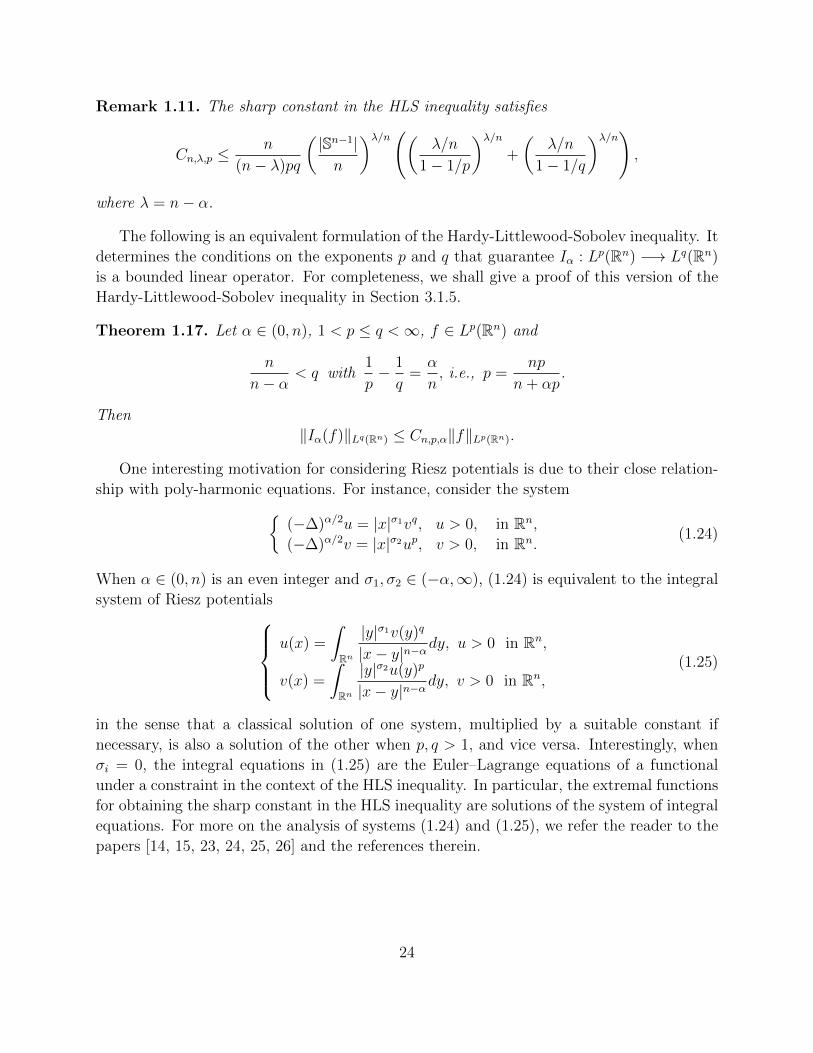
Remark 1.11. The sharp constant in the HLS inequality satisfies
Cn,λ,p ≤n
(n− λ)pq
(|Sn−1|n
)λ/n((λ/n
1− 1/p
)λ/n+
(λ/n
1− 1/q
)λ/n),
where λ = n− α.
The following is an equivalent formulation of the Hardy-Littlewood-Sobolev inequality. It
determines the conditions on the exponents p and q that guarantee Iα : Lp(Rn) −→ Lq(Rn)
is a bounded linear operator. For completeness, we shall give a proof of this version of the
Hardy-Littlewood-Sobolev inequality in Section 3.1.5.
Theorem 1.17. Let α ∈ (0, n), 1 < p ≤ q <∞, f ∈ Lp(Rn) and
n
n− α< q with
1
p− 1
q=α
n, i.e., p =
np
n+ αp.
Then
‖Iα(f)‖Lq(Rn) ≤ Cn,p,α‖f‖Lp(Rn).
One interesting motivation for considering Riesz potentials is due to their close relation-
ship with poly-harmonic equations. For instance, consider the system{(−∆)α/2u = |x|σ1vq, u > 0, in Rn,
(−∆)α/2v = |x|σ2up, v > 0, in Rn.(1.24)
When α ∈ (0, n) is an even integer and σ1, σ2 ∈ (−α,∞), (1.24) is equivalent to the integral
system of Riesz potentialsu(x) =
ˆRn
|y|σ1v(y)q
|x− y|n−αdy, u > 0 in Rn,
v(x) =
ˆRn
|y|σ2u(y)p
|x− y|n−αdy, v > 0 in Rn,
(1.25)
in the sense that a classical solution of one system, multiplied by a suitable constant if
necessary, is also a solution of the other when p, q > 1, and vice versa. Interestingly, when
σi = 0, the integral equations in (1.25) are the Euler–Lagrange equations of a functional
under a constraint in the context of the HLS inequality. In particular, the extremal functions
for obtaining the sharp constant in the HLS inequality are solutions of the system of integral
equations. For more on the analysis of systems (1.24) and (1.25), we refer the reader to the
papers [14, 15, 23, 24, 25, 26] and the references therein.
24

1.3.3 Green’s Function and Representation Formulas of Solutions
Let U ⊂ Rn be an open and bounded subset with C1 boundary ∂U . Our goal here is to find
a representation of the solution of Poisson’s equation
−∆u = f in U
subject to the prescribed boundary condition
u = g on ∂U.
We derive the formula for the Green’s function to this problem. Fix x ∈ U and choose ε > 0
suitably small so that Bε(x) ⊂ U . Then, apply Green’s formula on the region Vε = U\Bε(x)
to u(y) and Γ(y − x) to getˆVε
u(y)∆Γ(y−x)−Γ(y−x)∆u(y) dy =
ˆ∂Vε
u(y)∂Γ
∂ν(y−x)−Γ(y−x)
∂u
∂ν(y) dS(y). (1.26)
Notice that ∆Γ(x− y) = 0 for x 6= y and that∣∣∣ ˆ∂Bε(x)
Γ(y − x)∂u
∂ν(y) dS(y)
∣∣∣ ≤ Cεn−1 max∂Bε(0)
|Γ| = o(1).
Then, similar to the proof of Theorem 1.15, we can show thatˆ∂Bε(x)
u(y)∂Γ
∂ν(y − x) dS(y) =
1
|∂Bε(x)|
ˆ∂Bε(x)
u(y) dS(y) −→ u(x)
as ε −→ 0. Hence, sending ε −→ 0 in (1.26) yields
u(x) =
ˆ∂U
{Γ(y − x)
∂u
∂ν(y)− u(y)
∂Γ
∂ν(y − x)
}dS(y)−
ˆU
Γ(y − x)∆u(y) dy. (1.27)
Indeed, identity (1.27) holds for any point x ∈ U and any function u ∈ C2(U). This
representation of u is almost complete since we know u satisfies Poisson’s equation and
its values on the boundary are given, i.e., we know the values of ∆u in U and u = g on
∂U . However, we do not know a priori the value of ∂u/∂ν on ∂U . To circumvent this,
we introduce, for fixed x ∈ U , a corrector function φx = φx(y), solving the boundary-value
problem {∆φx = 0 in U,φx = Γ(y − x) on ∂U.
(1.28)
As before, if we apply Green’s formula once more, we obtain
−ˆU
φx(y)∆u(y) dy =
ˆ∂U
u(y)∂φx
∂ν(y)− φx(y)
∂u
∂ν(y) dS(y)
=
ˆ∂U
u(y)∂φx
∂ν(y)− Γ(y − x)
∂u
∂ν(y) dS(y). (1.29)
Now introduce the Green’s function for the region U .
25

Definition 1.4. The Green’s function for the region U is
G(x, y) := Γ(y − x)− φx(y) for x, y ∈ U, x 6= y.
In view of this definition, adding (1.29) to (1.27) yields
u(x) = −ˆ∂U
u(y)∂G
∂ν(x, y) dS(y)−
ˆU
G(x, y)∆u(y) dy (x ∈ U), (1.30)
where∂G
∂ν(x, y) = DyG(x, y) · ν(y)
is the outer normal derivative of G with respect to the variable y. Here, observe that the
term ∂u/∂ν no longer appears in identity (1.30).
In summary, suppose that u ∈ C2(U) is a solution of the boundary-value problem{−∆u = f in U,
u = g on ∂U,(1.31)
for given continuous functions f and g. Then, we have basically shown the following.
Theorem 1.18 (Representation formula via Green’s function). If u ∈ C2(U) solves problem
(1.31), then
u(x) = −ˆ∂U
g(y)∂G
∂ν(x, y) dS(y) +
ˆU
G(x, y)f(y) dy (x ∈ U). (1.32)
If the geometry of U is simple enough, then we can actually compute the corrector
function explicitly to obtain G. Two such examples are when U is the unit ball or the
hyperbolic or half-space in Rn.
1.3.4 Green’s Function for a Half-Space
Consider the half-space
Rn+ = {x = (x1, x2, . . . , xn) ∈ Rn |xn > 0},
whose boundary is given by ∂Rn+ = Rn−1. Although the half-space is unbounded and the
calculations in the previous section assumed U was bounded, we can still use the same ideas
to find the Green’s function for the half-space. In order to do so, we adopt a reflection
argument. Namely, if x = (x1, x2, . . . , xn) ∈ Rn+, we let x = (x1, x2, . . . ,−xn), the reflection
of x in the plane ∂Rn+. Then set
φx(y) = Γ(y − x) = Γ(y1 − x1, . . . , yn−1 − xn−1, yn + xn) for x, y ∈ Rn+.
26

The idea is that this corrector φx is built from Γ by reflecting the singularity from x ∈ Rn+
to x 6∈ Rn+. Observe that
φx(y) = Γ(y − x) if y ∈ ∂Rn+,
and thus {∆φx = 0 in Rn
+,φx = Γ(y − x) on ∂Rn
+,(1.33)
as required. That is, we have the following definition.
Definition 1.5. The Green’s function for the half-space Rn+ is
G(x, y) := Γ(y − x)− Γ(y − x) for x, y ∈ Rn+, x 6= y.
Then
Gyn(x, y) = Γyn(y − x)− Γyn(y − x) =−1
ωn
[ yn − xn|y − x|n
− yn + xn|y − x|n
].
Consequently, if y ∈ ∂Rn+,
∂G
∂ν(x, y) = −Gyn(x, y) = −2xn
ωn
1
|x− y|n.
Now if u solves the boundary-value problem{∆u = 0 in Rn
+,u = g on ∂Rn
+,(1.34)
then the representation formula (1.32) of the previous theorem suggests that
u(x) =2xnωn
ˆ∂Rn+
g(y)
|x− y|ndy (x ∈ Rn
+) (1.35)
is the representation formula for the solution. Here, the function
K(x, y) :=2xnωn
1
|x− y|nfor x ∈ Rn
+, y ∈ ∂Rn+
is called Poisson’s kernel for U = Rn+ and (1.35) is called Poisson’s formula. Now, let us
prove that Poisson’s formula indeed gives the formula for the solution of the boundary-value
problem (1.34).
Theorem 1.19 (Poisson’s formula for Rn+). Assume g ∈ C(Rn−1) ∩ L∞(Rn−1), and define
u by Poisson’s formula (1.35). Then
(a) u ∈ C∞(Rn+) ∩ L∞(Rn
+),
(b) ∆u = 0 in Rn+,
(c) limx→x0,x∈Rn+
u(x) = g(x0) for each point x0 ∈ ∂Rn+.
27

1.3.5 Green’s Function for a Ball
If U = B1(0), we construct the Green’s function through another reflection argument, but
here we exploit an inversion through the unit sphere ∂B1(0).
Definition 1.6. If x ∈ Rn\{0}, the point
x =x
|x|2
is called the point dual to x with respect to ∂B1(0). The mapping x 7→ x is inversion through
the unit sphere ∂B1(0).
Obviously, the inversion maps points on the sphere to itself, maps the points in the ball
to its exterior Rn\B1(0), and maps points in the exterior into the ball. Now fix x ∈ B1(0)
and we want to find the corrector function φx = φx(y) solving{∆φx = 0 in B1(0),φx = Γ(y − x) on ∂B1(0),
(1.36)
with the Green’s function
G(x, y) = Γ(y − x)− φx(y).
Notice that the mapping y 7→ Γ(y − x) is harmonic for y 6= x. Thus y 7→ |x|2−nΓ(y − x) is
harmonic for y 6= x. Hence,
φx(y) := Γ(|x|(y − x)) (1.37)
is harmonic in U = B1(0). Furthermore, if y ∈ ∂B1(0) and x 6= 0,
|x|2|y − x|2 = |x|2(|y|2 − 2
y · x|x|2
+1
|x|2)
= |x|2 − 2y · x+ 1 = |x− y|2.
That is, |x− y|2−n = (|x||y − x|)2−n and so
φx(y) = Γ(y − x) (y ∈ ∂B1(0)),
as required.
Definition 1.7. The Green’s function for the unit ball B1(0) is
G(x, y) := Γ(y − x)− Γ(|x|(y − x)) (x, y ∈ B1(0)). (1.38)
Note that the same formula holds when n = 2, where the kernel Γ is of the logarithmic
type. Now assume u solves the boundary-value problem{∆u = 0 in B1(0),u = g on ∂B1(0).
(1.39)
28
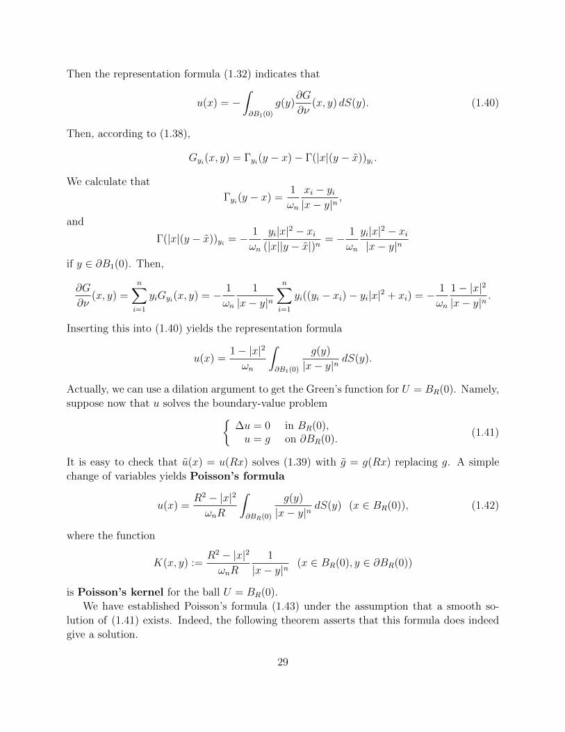
Then the representation formula (1.32) indicates that
u(x) = −ˆ∂B1(0)
g(y)∂G
∂ν(x, y) dS(y). (1.40)
Then, according to (1.38),
Gyi(x, y) = Γyi(y − x)− Γ(|x|(y − x))yi .
We calculate that
Γyi(y − x) =1
ωn
xi − yi|x− y|n
,
and
Γ(|x|(y − x))yi = − 1
ωn
yi|x|2 − xi(|x||y − x|)n
= − 1
ωn
yi|x|2 − xi|x− y|n
if y ∈ ∂B1(0). Then,
∂G
∂ν(x, y) =
n∑i=1
yiGyi(x, y) = − 1
ωn
1
|x− y|nn∑i=1
yi((yi − xi)− yi|x|2 + xi) = − 1
ωn
1− |x|2
|x− y|n.
Inserting this into (1.40) yields the representation formula
u(x) =1− |x|2
ωn
ˆ∂B1(0)
g(y)
|x− y|ndS(y).
Actually, we can use a dilation argument to get the Green’s function for U = BR(0). Namely,
suppose now that u solves the boundary-value problem{∆u = 0 in BR(0),u = g on ∂BR(0).
(1.41)
It is easy to check that u(x) = u(Rx) solves (1.39) with g = g(Rx) replacing g. A simple
change of variables yields Poisson’s formula
u(x) =R2 − |x|2
ωnR
ˆ∂BR(0)
g(y)
|x− y|ndS(y) (x ∈ BR(0)), (1.42)
where the function
K(x, y) :=R2 − |x|2
ωnR
1
|x− y|n(x ∈ BR(0), y ∈ ∂BR(0))
is Poisson’s kernel for the ball U = BR(0).
We have established Poisson’s formula (1.43) under the assumption that a smooth so-
lution of (1.41) exists. Indeed, the following theorem asserts that this formula does indeed
give a solution.
29

Theorem 1.20 (Poisson’s formula for the ball BR(0)). Assume g ∈ C(∂BR(0)) and define
u by Poisson’s formula (1.43). Then
(a) u ∈ C∞(BR(0)),
(b) ∆u = 0 in BR(0),
(c) limx→x0,x∈BR(0)
u(x) = g(x0) for each point x0 ∈ ∂BR(0).
Observe that Harnack’s inequality can be established directly from Poisson’s formula
(1.43).
Theorem 1.21 (Harnack’s inequality). Suppose u is a non-negative harmonic function in
BR(x0). Then ( R
R + r
)n−2R− rR + r
u(x0) ≤ u(x) ≤( R
R− r
)n−2R + r
R− ru(x0)
where r = |x− x0| < R.
Proof. By the regularity and translation invariance properties of harmonic functions, we may
assume x0 = 0 and u ∈ C(BR). Thus, from Poisson’s formula,
u(x) =R2 − |x|2
ωnR
ˆ∂BR(0)
u(y)
|x− y|ndS(y) (x ∈ BR(0)). (1.43)
Now, since R− |x| ≤ |x− y| ≤ R + |x| for |y| = R, we obtain
1
ωnR
R− |x|R + |x|
( 1
R + |x|
)n−2ˆ∂BR
u(y) dS ≤ u(x) ≤ 1
ωnR
R + |x|R− |x|
( 1
R− |x|
)n−2ˆ∂BR
u(y) dS.
In view of the mean value property,
u(0) =1
ωnRn−1
ˆ∂BR
u(y) dS,
we insert this into the previous estimates to arrive at the desired result.
From this, we deduce the Liouville theorem.
Corollary 1.4. If u is an entire function, i.e., it is harmonic in U = Rn, and u is either
bounded above or below, then u is necessarily constant.
Proof. By shifting, we may assume u is non-negative in Rn. Then take any point x ∈ Rn
and apply the previous Harnack’s inequality to u on any ball BR(0) with |x| < R to get( R
R + |x|
)n−2R− |x|R + |x|
u(0) ≤ u(x) ≤( R
R− |x|
)n−2R + |x|R− |x|
u(0).
Sending R −→ +∞ here yields u(x) = u(0), and we conclude that u is constant everywhere
in Rn since x was chosen arbitrarily.
30

1.4 Holder Regularity for Poisson’s Equation
Let us motivate the consideration of Holder spaces Ck,α rather than the classical Ck spaces
when dealing with regularity and solvability of elliptic problems of the form Lu = f in U .
For instance, if f ∈ C∞0 (U) and Γ = Γ(x) is the fundamental solution of Laplace’s
equation, then the Newtonian potential of f , i.e., w = Γ ∗ f or
w(x) =
ˆU
Γ(x− y)f(y) dy,
belongs to C∞(U). However, if f is merely just continuous, then w is not necessarily twice
differentiable.
Generally, Lu = f in U is uniquely solvable for all f ∈ C2(U) in that there exists a unique
solution u ∈ C2(U) for each such f ; namely, the elliptic operator L : C2(U) → C2(U) is a
bijective mapping. On the other hand, we naturally ask if for every f ∈ C(U) the equation
Lu = f has a solution u in C2(U). Interestingly enough, this is not true and so the mapping
L : C2(U) → C(U) is not bijective. For instance, if L = −∆ or L = −(∆ − 1) and for the
equation Lu = f , it is not true that for every f ∈ C(U) the corresponding solution u belongs
in C2(U) (see the example given below). Fortunately, if we hope to recover the bijectivity
of the map L, we must instead consider the Holder space Cα(U) in place of C(U).
Remark 1.12. One instance where the bijectivity (namely, the invertibility) of the map L
becomes very important is in the method of continuity (see Section 2.6). This method makes
use of the bijection of the solution map and the global C2,α regularity estimates to prove
existence results to general elliptic boundary value problems. Therefore, this gives further
motivation and a glimpse of some topics examined in the later chapters.
Example: Let us provide an example in which the solvability of −∆u = f for a carefully
chosen continuous f fails within the class of C2 solutions. Take the continuous but not
Holder continuous function
f(x) =x2
1 − x22
2|x|2( n+ 2
(− log |x|)1/2+
1
2(− log |x|)3/2
),
set
g(x) =√− logR(x2
2 − x21),
and let U = BR(0) with R < 1. Then
u(x) = (x22 − x2
1)(− log |x|)1/2
belongs to C(BR(0)) ∩ C∞(BR(0)\{0}) and satisfies{−∆u = f in BR(0)\{0},
u = g on ∂BR(0),(1.44)
31
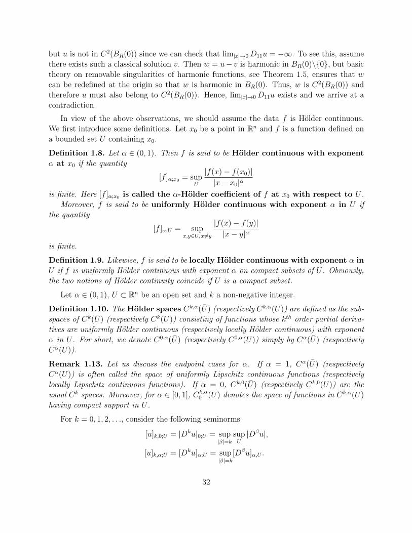
but u is not in C2(BR(0)) since we can check that lim|x|→0D11u = −∞. To see this, assume
there exists such a classical solution v. Then w = u− v is harmonic in BR(0)\{0}, but basic
theory on removable singularities of harmonic functions, see Theorem 1.5, ensures that w
can be redefined at the origin so that w is harmonic in BR(0). Thus, w is C2(BR(0)) and
therefore u must also belong to C2(BR(0)). Hence, lim|x|→0D11u exists and we arrive at a
contradiction.
In view of the above observations, we should assume the data f is Holder continuous.
We first introduce some definitions. Let x0 be a point in Rn and f is a function defined on
a bounded set U containing x0.
Definition 1.8. Let α ∈ (0, 1). Then f is said to be Holder continuous with exponent
α at x0 if the quantity
[f ]α;x0 = supU
|f(x)− f(x0)||x− x0|α
is finite. Here [f ]α;x0 is called the α-Holder coefficient of f at x0 with respect to U .
Moreover, f is said to be uniformly Holder continuous with exponent α in U if
the quantity
[f ]α;U = supx,y∈U, x6=y
|f(x)− f(y)||x− y|α
is finite.
Definition 1.9. Likewise, f is said to be locally Holder continuous with exponent α in
U if f is uniformly Holder continuous with exponent α on compact subsets of U . Obviously,
the two notions of Holder continuity coincide if U is a compact subset.
Let α ∈ (0, 1), U ⊂ Rn be an open set and k a non-negative integer.
Definition 1.10. The Holder spaces Ck,α(U) (respectively Ck,α(U)) are defined as the sub-
spaces of Ck(U) (respectively Ck(U)) consisting of functions whose kth order partial deriva-
tives are uniformly Holder continuous (respectively locally Holder continuous) with exponent
α in U . For short, we denote C0,α(U) (respectively C0,α(U)) simply by Cα(U) (respectively
Cα(U)).
Remark 1.13. Let us discuss the endpoint cases for α. If α = 1, Cα(U) (respectively
Cα(U)) is often called the space of uniformly Lipschitz continuous functions (respectively
locally Lipschitz continuous functions). If α = 0, Ck,0(U) (respectively Ck,0(U)) are the
usual Ck spaces. Moreover, for α ∈ [0, 1], Ck,α0 (U) denotes the space of functions in Ck,α(U)
having compact support in U .
For k = 0, 1, 2, . . ., consider the following seminorms
[u]k,0;U = |Dku|0;U = sup|β|=k
supU|Dβu|,
[u]k,α;U = [Dku]α;U = sup|β|=k
[Dβu]α,U .
32

With these seminorms, we can define the norms
‖u‖Ck(U) = |u|k;U = |u|k,0;U =k∑j=0
[u]j,0;U =k∑j=0
|Dju|0;U ,
‖u‖Ck,α(U) = |u|k,α;U = |u|k;U + [u]k,α;U = |u|k;U + [Dku]α;U ,
on the spaces Ck(U), Ck,α(U). It is sometimes useful, especially in this section anyway,
to consider non-dimensional norms on these spaces. In particular, if U is bounded with
d = diam(U), we set
‖u‖′Ck(U) = |u|′k;U =k∑j=0
dj[u]j,0;U =k∑j=0
dj|Dju|0;U ,
‖u‖′Ck,α(U) = |u|′k,α;U = |u|′k;U + dk+α[u]k,α;U = |u|′k;U + dk+α[Dku]α;U .
Not surprisingly, we have the following basic result, which we give without proof.
Theorem 1.22. Let α ∈ [0, 1] and U ⊂ Rn be an open domain. The spaces Ck(U), Ck,α(U)
equipped with the norms defined above are Banach spaces.
The following algebra property holds: the product of Holder continuous functions is
again Holder continuous. Namely, if u ∈ Cα(U), v ∈ Cβ(U), we have uv ∈ Cγ(U) where
γ = min{α, β}, and
‖uv‖Cγ(U) ≤ max(1, dα+β−2γ)‖u‖Cα(U)‖v‖Cβ(U),
‖uv‖′Cγ(U) ≤ ‖u‖′
Cα(U)‖v‖′
Cβ(U).
1.4.1 The Dirichlet Problem for Poisson’s Equation
We now develop the regularity properties of Newtonian potentials. We will use this to
then show that Poisson’s equation in a bounded domain U may be solved under the same
boundary conditions for which Laplace’s equation is solvable.
Lemma 1.5. Let f be a bounded and integrable in U , and let w be the Newtonian potential
of f . Then w ∈ C1(Rn) and for any x ∈ U ,
Diw(x) =
ˆU
DiΓ(x− y)f(y) dy, i = 1, 2, . . . , n.
Proof. It is easy to check the following derivative estimates for Γ:|DiΓ(x− y)| ≤ 1
nωn|x− y|1−n,
|DijΓ(x− y)| ≤ 1
ωn|x− y|−n,
|DβΓ(x− y) ≤ C(n, |β|)|x− y|2−n−|β|.
(1.45)
33

From this, the function
v(x) =
ˆU
DiΓ(x− y)f(y) dy
is well-defined. We now show that v = Diw. To do so, for ε > 0, let ηε(x, y) = η(|x− y|/ε)where η = η(|x|) is some non-negative radial function in C1(R) with supp(η) ⊆ [0, 1],
supp(η′) ⊆ [0, 2], and
η(|x|) :=
{0, if |x| ≤ 1,1, if |x| ≥ 2.
Define
wε(x) =
ˆU
ηε(x, y)Γ(x− y)f(y) dy,
which is obviously in C1(Rn). Then, there holds,
v(x)−Diwε(x) =
ˆB2ε(x)
Di
[(1− ηε(x, y))Γ(x− y)
]f(y) dy.
Hence, if n ≥ 3,
|v(x)−Diwε(x)| ≤ ‖f‖∞ˆB2ε(x)
|DiΓ(x− y)|+ 2
ε|Γ(x− y)| dy ≤ 2nε
n− 2‖f‖∞.
Note that if n = 2, it follows that
|v(x)−Diwε(x)| ≤ 4ε(1 + | ln 2ε|).
In either case, we conclude that as ε −→ 0, wε and Diwε converge uniformly on compact
subsets of Rn to w and v, respectively. Therefore, w ∈ C1(Rn) and v = Diw.
Lemma 1.6. Let f be bounded and locally Holder continuous in U with exponent α ∈ (0, 1],
and let w be the Newtonian potential of f . Then
(a) w ∈ C2(U);
(b) −∆w = f in U ;
(c) For any x ∈ U ,
Dijw(x) =
ˆU0
DijΓ(x−y)(f(y)−f(x)) dy−f(x)
ˆ∂U0
DiΓ(x−y)νj(y) dSy, i, j = 1, 2, . . . , n.
(1.46)
Here, U0 is any domain containing U for which the divergence theorem holds and f is extended
to vanish outside U .
34

Proof. Using the derivative estimates of (1.45) for D2Γ and since f is pointwise Holder
cotinuous in U , the function
u(x) =
ˆU0
DijΓ(x− y)(f(y)− f(x)) dy − f(x)
ˆ∂U0
DiΓ(x− y)νj(y) dSy,
is well-defined. Let v = Diw and define for ε > 0,
vε(x) =
ˆU
DiΓ(x− y)ηε(x, y)f(y) dy,
where ηε is the same test function as in the previous lemma. Obviously, vε ∈ C1(U) and for
ε > 0 sufficiently small, differentiating leads to
Djvε(x) =
ˆU
Dj(DiΓ(x− y)ηε(x, y))f(y) dy
=
ˆU
Dj(DiΓ(x− y)ηε(x, y))(f(y)− f(x)) dy + f(x)
ˆU0
Dj(DiΓ(x− y)ηε(x, y)) dy
=
ˆU
Dj(DiΓ(x− y)ηε(x, y))(f(y)− f(x)) dy + f(x)
ˆ∂U0
DiΓ(x− y)νj(y) dSy.
Hence, by subtracting this from u(x), we estimate that
|u(x)−Djvε(x)| =∣∣∣ˆ
B2ε(x)
Dj[(1− ηε)DiΓ(x− y)](f(y)− f(x)) dy∣∣∣
≤ [f ]α;x
ˆB2ε(x)
(|DijΓ|+
2
ε|DiΓ|
)|x− y|α dy
≤(nα
+ 4)
(2ε)α[f ]α;x,
provided that 2ε < dist(x, ∂U). Therefore, Djvε converges to u uniformly on compact subsets
of U as ε −→ 0. Of course, vε converges to v = Diw as ε −→ 0. Hence, w ∈ C2(U) and
u = Dijw. Then, if we set U0 = Br(x) for r suitably large,
−∆w(x) =1
ωnrn−1f(x)
ˆ∂Br(x)
νi(y)νi(y) dSy = f(x).
This completes the proof of the lemma.
A consequence of Lemmas 1.5 and 1.6 is the following theorem. This result should be
compared with Theorem 1.15 as it generalizes that result in that f is assumed to be bounded
and locally Holder continuous in U rather than the stronger condition that f ∈ C2c (U).
Theorem 1.23. Let U be a bounded domain and suppose that each point of ∂U is regular
(with respect to the Laplacian). Then, if f is a bounded, locally Holder continuous function
in U , the classical Dirichlet problem{−∆u = f in U,
u = g on ∂U,(1.47)
35

is uniquely solvable for any continuous boundary values g in the class of classical solutions,
i.e., u ∈ C2(U) ∩ C(U).
Proof. Let w be the Newtonian potential of f and consider the function v = u−w. It is clear
that −∆v = 0 in U and v = g − w on ∂U , but it is obvious that the unique solvability of
this boundary-value problem for Laplace’s equation will imply the desired result. Now, the
existence of classical solutions of Laplace’s equation follows from several methods, e.g. the
Perron method, which are provided in the next chapter, and the uniqueness of the solution
is a consequence of the maximum principles.
Remark 1.14. Here, a boundary point will be called regular (with respect to the Laplacian)
if there exists a barrier function at that point. For the definition of a barrier function, see
(2.22) in the next chapter discussing Perron’s method. There we shall see that if ∂U is C2
then each point on the boundary is indeed regular. Furthermore, the regularity theory below
indicates that the unique solution of the above Dirichlet problem on a Euclidean ball domain
belongs to C2,α(U) ∩ C(U)
Remark 1.15. If U = BR(0), the last theorem follows from the two preceding lemmas and
Poisson’s formula (1.43) for the ball. In fact, we even have an explicit representation of the
unique solution, which is given by
u(x) =
ˆ∂BR(0)
K(x, y)g(y) dSy +
ˆBR(0)
G(x, y)f(y) dy,
where K(x, y) and G(x, y) = Γ(y− x)− φx(y) are Poisson’s kernel and the Green’s function
on the ball, respectively. In particular, for all x, y ∈ BR(0), x 6= y,
G(x, y) = Γ(√
(|x||y|/2)2 +R2 − 2x · y)− Γ(√|x|2 + |y|2 − 2x · y). (1.48)
1.4.2 Interior Holder Estimates for Second Derivatives
For concentric balls of radius R > 0 centered at x0 in Rn, we set B1 = BR(x0) and B2 =
B2R(x0).
Lemma 1.7. Suppose that f ∈ Cα(B2), α ∈ (0, 1), and let w be the Newtonian potential of
f in B2. Then w ∈ C2,α(B1) and
|D2w|′0,α;B1≤ C(n, α)|f |′0,α;B2
,
|D2w|0;B1 +Rα[D2w]α;B1 ≤ C(n, α)(|f |0;B2 +Rα[f ]α;B2).
Remark 1.16. For general domains U1 ⊂ B1(x0) and B2(x0) ⊂ U2, and f ∈ Cα(U2) and w
is the Newtonian potential of f over U2. Then the statement of Lemma 1.7 with Ui replacing
Bi(x0), i = 1, 2, respectively, still remains true.
36

Proof of Lemma 1.7. For any x ∈ B1, identity (1.46) yields
Dijw(x) =
ˆB2
DijΓ(x− y)[f(y)− f(x)] dy − f(x)
ˆ∂B2
DiΓ(x− y)νj(y) dSy (1.49)
and thus, by the derivative estimates in (1.45),
|Dijw(x)| ≤ |f(x)|nωn
R1−nˆ∂B2
dSy +[f ]α;x
ωn
ˆB2
|x− y|α−n dy
= 2n−1|f(x)|+ n
α(3R)α[f ]α;x ≤ C(n, α)(|f(x)|+Rα[f ]α;x). (1.50)
Then, again (1.46) implies that for any other point x ∈ B1 we have
Dijw(x) =
ˆB2
DijΓ(x− y)[f(y)− f(x)] dy − f(x)
ˆ∂B2
DiΓ(x− y)νj(y) dSy. (1.51)
Set δ = |x− x| and ξ = (x+ x)/2. Subtracting (1.51) from (1.49) yields
Dijw(x)−Dijw(x) = f(x)I1 + [f(x)− f(x)]I2 + I3 + I4 + [f(x)− f(x)]I5 + I6,
where
I1 =
ˆ∂B2
[DiΓ(x− y)−DiΓ(x− y)]νj(y) dSy,
I2 =
ˆ∂B2
DiΓ(x− y)νj(y) dSy,
I3 =
ˆBδ(ξ)
DijΓ(x− y)[f(x)− f(y)] dy,
I4 =
ˆBδ(ξ)
DijΓ(x− y)[f(y)− f(x)] dy,
I5 =
ˆB2\Bδ(ξ)
DijΓ(x− y) dy,
I6 =
ˆB2\Bδ(ξ)
[DijΓ(x− y)−DijΓ(x− y)][f(x)− f(y)] dy.
We estimate each term Ii: For some x between x and x,
|I1| ≤ |x− x|ˆ∂B2
|DDiΓ(x− y)| dSy
≤ n22n−1|x− x|R
(since |x− y| ≥ R for y ∈ ∂B2)
≤ n22n−α( δR
)α(since δ = |x− x| < 2R).
37

|I2| ≤1
nωnR1−n
ˆ∂B2
dSy = 2n−1.
|I3| ≤ˆBδ(ξ)
|DijΓ(x− y)||f(x)− f(y)| dy ≤ 1
ωn[f ]α;x
ˆB(3/2)δ(x)
|x− y|α−n dy ≤ n
α
(3δ
2
)α[f ]α;x.
Similarly,
|I4| ≤n
α
(3δ
2
)α[f ]α;x.
|I5| =∣∣∣ ˆ
∂(B2\Bδ(ξ))DiΓ(x− y)νj(y) dSy
∣∣∣≤∣∣∣ˆ
∂B2
DiΓ(x− y)νj(y) dSy
∣∣∣+∣∣∣ ˆ
∂Bδ(ξ)
DiΓ(x− y)νj(y) dSy
∣∣∣≤ 2n−1 +
1
nωn
(δ2
)1−nˆ∂Bδ(ξ)
dSy = 2n−1 + 2n−1 = 2n.
|I6| ≤ |x− x|ˆB2\Bδ(ξ)
|DDijΓ(x− y)||f(x)− f(y)| dy (for some x between x and x)
≤ c(n)δ
ˆ|y−ξ|≥δ
|f(x)− f(y)||x− y|n+1
dy
≤ cδ[f ]α;x
ˆ|y−ξ|≥δ
|ξ − y|α−n−1 dy (since |x− y| ≤ (3/2)|ξ − y| ≤ 3|x− y|)
≤ c(n)(1− α)−12n+1(3
2
)αδα[f ]α;x.
Combining these estimates gives us
|Dijw(x)−Dijw(x)| ≤ C(n, α)(R−α|f(x)|+ [f ]α;x + [f ]α;x
)|x− x|α.
Hence, this along with (1.50) completes the proof of the lemma.
Theorem 1.24. Let f ∈ Cα0 (Rn) and suppose u ∈ C2
0(Rn) satisfy Poisson’s equation,
−∆u = f in Rn.
Then u ∈ C2,α0 (Rn), and if B = BR(x0) is any ball containing the support of u, then
|D2u|′0,α;B ≤ C(n, α)|f |′0,α;B,
|u|′1,B ≤ C(n)R2|f |0;B.
38

Proof. As indicated in Theorem 1.15 or Lemma 1.6, we can conclude that u = Γ ∗ f , even
if it was assumed there that f ∈ C2c (Rn) as it still holds true even when f ∈ Cα
0 (Rn). The
estimates for Du and D2u follow, respectively, from Lemma 1.5 and Lemma 1.7 and the fact
that f has compact support. The estimate for |u|0;B follows at once from that for Du.
The restriction that u and f have compact support in the last theorem can be removed.
Theorem 1.25. Let U be a domain in Rn and let f ∈ Cα(U), α ∈ (0, 1), and let u ∈ C2(U)
satisfy Poisson’s equation, −∆u = f in U . Then u ∈ C2,α(U) and for any two concentric
balls BR(x0), B2R(x0) ⊂⊂ U , we have
|u|′2,α;BR(x0) ≤ C(n, α)(|u|0;B2R(x0) +R2|f |′0,α;B2R(x0)). (1.52)
A consequence of the interior estimate (1.52) is the equicontinuity on compact subsets
of the second derivatives of any bounded set of solutions of Poisson’s equation. Therefore,
the Arzela–Ascoli theorem implies the following result on the compactness of solutions to
Poisson’s equation.
Corollary 1.5. Any bounded sequence of solutions of Poisson’s equation, −∆u = f in U ,
where f ∈ Cα(U), contains a subsequence converging uniformly on compact subsets of U to
another solution.
As a consequence of this compactness result, we establish an existence result for the
Dirichlet problem. Here, we denote dx = dx(U) = dist(x, ∂U).
Theorem 1.26. Let B be a ball in Rn and f be a function in Cα(B) for which
supx∈B
d2−βx |f(x)| ≤ N <∞
for some β ∈ (0, 1). Then there exists a unique function u ∈ C2(B) ∩ C(B) satisfying{−∆u = f in B,
u = 0 on ∂B.
Furthermore, the solution u satisfies the estimate
supx∈B
d−βx |u(x)| ≤ CN, (1.53)
where C = C(β).
Proof. Step 1: Estimate (1.53) follows from a simple barrier argument, i.e., let B = BR(x0),
r = |x− x0| and set w(x) = (R2 − r2)β. A direct calculation will show that
∆w(x) = − 2β(R2 − r2)β−2[n(R2 − r2) + 2(1− β)r2]
≤ − 4β(1− β)R2(R2 − r2)β−2 ≤ −β(1− β)Rβ(R− r)β−2.
39

Now suppose that −∆u = f in B and u = 0 on ∂B. Since dx = R− r, the hypothesis yields
|f(x)| ≤ Ndβ−2x = N(R− r)β−2 ≤ −C0N∆w,
where C0 = [β(1− β)Rβ]−1. Hence,
−∆(C0Nw ± u) ≥ 0 in B, and C0Nw ± u = 0 on ∂B.
Therefore, the maximum principle implies
|u(x)| ≤ C0Nw(x) ≤ CNdβx for x ∈ B, (1.54)
which implies (1.53) with constant C = 2/β(1− β).
Step 2: We now prove the existence of u. Define
fm =
m, if f ≥ m,f, if |f | ≤ m,−m, if f ≤ −m,
and let {Bk} be a sequence of concentric balls exhausting B such that |f | ≤ k in Bk. We
define um to be the solution of −∆um = fm in B and um = 0 on ∂B. By (1.53),
supx∈B
d−βx |um(x)| ≤ C supx∈B
d2−βx |fm(x)| ≤ CN,
so that the sequence {um} is uniformly bounded and −∆um = f in Bk for m ≥ k. Hence, by
Corollary 1.5 applied successively to the sequence of balls Bk, we can extract a convergent
subsequence of {um} with limit point u in C2(B) satisfying −∆u = f in B. Moreover, there
holds |u(x)| ≤ CNdβx and so u = 0 on ∂B. This completes the proof of the theorem.
1.4.3 Boundary Holder Estimates for Second Derivatives
We may refine the interior Holder regularity estimates by extending them up to the boundary.
We focus only on ball domains but the results certainly apply to bounded and open domains
with smooth boundary. We refer the reader to Chapter 3 for more details on obtaining
regularity estimates up to the boundary for general smooth domains.
We start with some notation. Let Rn+ := {x ∈ Rn |xn > 0} be the usual upper half-space
with boundary T = ∂Rn+, B2 := B2R(x0), B1 = BR(x0) where R > 0 and x0 ∈ Rn
+. Moreover,
set B+2 := B2 ∩ Rn
+ and B+1 = B1 ∩ Rn
+.
Lemma 1.8. Let f ∈ Cα(B+2 ) and let w be the Newtonian potential of f in B+
2 . Then
w ∈ C2,α(B+1 ) and
|D2w|′0,α;B+
1≤ C|f |′
0,α;B+2
(1.55)
where C = C(n, α).
40

Proof. We may assume B2 intersects T , otherwise the result is already contained in Lemma
1.7. The representation (1.46) holds for Dijw within U0 = B+2 . If either i or j 6= n, then the
portion of the boundary integralˆ∂B+
2
DiΓ(x− y)νj(y) dSy =
ˆ∂B+
2
DjΓ(x− y)νi(y) dSy
on T vanishes since νi or νj equals to 0 there. The estimates in Lemma 1.7 for Dijw (i
or j 6= 0) then proceed exactly as before with B2 replaced with B+2 , Bδ(ξ) replaced by
Bδ(ξ)∩B+2 and ∂B2 replaced by ∂B+
2 \T . Finally, Dnnw can be estimated from the equation
−∆w = f and the estimates Dkkw for k = 1, 2, . . . , n− 1.
Theorem 1.27. Let u ∈ C2(B+2 )∩C(B+
2 ), f ∈ Cα(B+2 ), satisfy −∆u = f in B+
2 , u = 0 on
T . Then u ∈ C2,α(B+1 ) and we have
|u|′2,α;B+
1≤ C(|u|0;B+
2+R2|f |′
0,α;B+2
) (1.56)
where C = C(n, α).
Proof. Let x′ = (x1, x2, . . . , xn−1), x∗ = (x′,−xn) and define
f ∗(x) = f ∗(x′, xn) :=
{f(x′, xn), if xn ≥ 0,f(x′,−xn), if xn ≤ 0.
We assume that B2 intersects T ; otherwise Theorem 1.7 already implies estimate (1.56).
Now set B−2 := {x ∈ Rn |x∗ ∈ B+2 } and D = B+
2 ∪ B−2 ∪ (B2 ∩ T ). Then f ∗ ∈ Cα(D) and
|f ∗|′0,α;B+
2
.
Define
w(x) =
ˆB+
2
[Γ(x− y)− Γ(x∗ − y)]f(y) dy
=
ˆB+
2
[Γ(x− y)− Γ(x− y∗)]f(y) dy, (1.57)
so that w(x′, 0) = 0 and −∆w = f in B+2 . Observe that
ˆB+
2
Γ(x− y∗)f(y) dy =
ˆB−2
Γ(x− y)f ∗(y) dy,
so then we get
w(x) = 2
ˆB+
2
Γ(x− y)f(y) dy −ˆD
Γ(x− y)f ∗(y) dy.
Letting
w∗(x) =
ˆD
Γ(x− y)f ∗(y) dy,
41
the remark following Lemma 1.7 with U1 = B+1 and U2 = D implies that
|D2w∗|′0,α;B+
1≤ C|f ∗|′0,α;D ≤ 2C|f |′
0,α;B+2.
Combining this with Lemma 1.8 yields
|D2w|′0,α;B+
1≤ C|f |′
0,α;B+2.
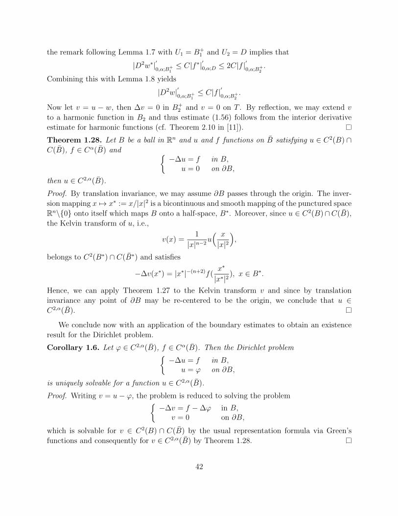
Now let v = u − w, then ∆v = 0 in B+2 and v = 0 on T . By reflection, we may extend v
to a harmonic function in B2 and thus estimate (1.56) follows from the interior derivative
estimate for harmonic functions (cf. Theorem 2.10 in [11]).
Theorem 1.28. Let B be a ball in Rn and u and f functions on B satisfying u ∈ C2(B) ∩C(B), f ∈ Cα(B) and {
−∆u = f in B,u = 0 on ∂B,
then u ∈ C2,α(B).
Proof. By translation invariance, we may assume ∂B passes through the origin. The inver-
sion mapping x 7→ x∗ := x/|x|2 is a bicontinuous and smooth mapping of the punctured space
Rn\{0} onto itself which maps B onto a half-space, B∗. Moreover, since u ∈ C2(B)∩C(B),
the Kelvin transform of u, i.e.,
v(x) =1
|x|n−2u( x
|x|2),
belongs to C2(B∗) ∩ C(B∗) and satisfies
−∆v(x∗) = |x∗|−(n+2)f(x∗
|x∗|2), x ∈ B∗.
Hence, we can apply Theorem 1.27 to the Kelvin transform v and since by translation
invariance any point of ∂B may be re-centered to be the origin, we conclude that u ∈C2,α(B).
We conclude now with an application of the boundary estimates to obtain an existence
result for the Dirichlet problem.
Corollary 1.6. Let ϕ ∈ C2,α(B), f ∈ Cα(B). Then the Dirichlet problem{−∆u = f in B,
u = ϕ on ∂B,
is uniquely solvable for a function u ∈ C2,α(B).
Proof. Writing v = u− ϕ, the problem is reduced to solving the problem{−∆v = f −∆ϕ in B,
v = 0 on ∂B,
which is solvable for v ∈ C2(B) ∩ C(B) by the usual representation formula via Green’s
functions and consequently for v ∈ C2,α(B) by Theorem 1.28.
42

CHAPTER 2
Existence Theory
2.1 The Lax-Milgram Theorem
Theorem 2.1 (Lax–Milgram). Let H be a Hilbert space with norm ‖·‖ and B : H×H −→ Ris a bilinear form. Suppose that there exist numbers α, β > 0 such that for any u, v ∈ H
(i) Boundedness: |B[u, v]| ≤ α‖u‖ · ‖v‖,
(ii) Coercivity: β‖u‖2 ≤ B[u, u],
then for each f ∈ L2(U) there exists a unique u ∈ H such that
B[u, v] = (f, v) for all v ∈ H.
To prove the theorem, we first recall the Riesz representation theorem for Hilbert spaces.
Theorem 2.2 (Riesz representation). If f is a bounded linear functional on a Hilbert Space
H with inner product (·, ·), then there exists an element v ∈ H such that < f, u >= (v, u)
for all u ∈ H.
It is clear that the inner product is a bilinear form which satisfies both the requirements of
the Lax–Milgram theorem. However, the Lax–Milgram theorem is a stronger result than the
Riesz representation theorem in that it does not require the bilinear form to be symmetric.
Proof. Existence: For each fixed w ∈ H, v −→ B[w, v] is a bounded linear functional on H.
By the Riesz representation theorem, there exists a u ∈ H such that (u, v) = B[w, v] for all
v ∈ H. We define the operator A : H −→ H by u = A[w].
43

Step 1: Claim that A : H −→ H is a bounded linear operator: To prove A is linear, observe
that
(A[λ1u1 + λ2u2], v) = B[λ1u1 + λ2u2, v] = λ1B[u1, v] + λ2B[u2, v]
= (λ1A[u1] + λ2A[u2], v) for all v ∈ H.
Thus, A[λ1u1 + λ2u2] = λ1A[u1] + λ2A[u2].
Moreover, A is bounded since
‖Au‖2 = (Au, Au) = B[Au, u] ≤ α‖u‖ · ‖Au‖
Hence, ‖Au‖ ≤ α‖u‖.
Step 2: Claim Ran(A) is closed in H.
Let {yk} be a convergent sequence in ran(A) so that there is a sequence {uk} ⊂ H for which
yk = A[uk] −→ y ∈ H. By coercivity, ‖uk − uj‖ ≤ β‖A[uk]−A[uj]‖, which implies {uk} is a
Cauchy sequence in H. Hence, uk converges to some element u ∈ H and y = A[u]; that is,
y ∈ Ran(A), thereby proving Ran(A) is closed in H.
Step 3: Claim Ran(A) = H.
On the contrary, assume that Ran(A) 6= H. Thus, we have that H = ran(A) ⊕ ran(A)⊥
since Ran(A) is closed, and we choose a non-zero element z ∈ ran(A)⊥. By the coercivity
condition, β‖z‖2 ≤ B[z, z] = (Az, z) = 0 and we arrive at a contradiction.
Step 4: For each f ∈ L2, the Riesz representation theorem once again implies there exists an
element z ∈ H for which (z, v) =< f, v > for all v ∈ H. In turn, we can find a u such that
z = A[u], i.e., (z, v) = (Au, v) = B[u, v] for all v ∈ H. Hence, we have found an element
u ∈ H for which B[u, v] = (f, v) for all v ∈ H.
Uniqueness: Suppose that u1 and u2 are two such elements satisfying B[u1, v] = (f, v) and
B[u2, v] = (f, v) for all v ∈ H, respectively. This implies that B[u1−u2, v] = 0 for all v ∈ H.
Now, if v = u1 − u2, the coercivity condition implies β‖u1 − u2‖2 ≤ B[u1 − u2, u1 − u2] = 0.
Hence, u1 = u2.
2.1.1 Existence of Weak Solutions
Our goal here is to prove existence and uniqueness of weak solutions to the Dirichlet boundary
value problem of the following form:{Lu+ µu = f in U,
u = 0 on ∂U,(2.1)
where µ is a non-negative constant to be determined later. Developing this result relies
mainly on certain energy estimates and the Lax-Milgram theorem. In addition, we will now
44

focus strictly on the second order differential operator in divergence form with its associated
bilinear form
B[u, v] :=
ˆU
n∑i,j=1
aij(x)DiuDjv +n∑i=1
bi(x)Diuv + c(x)uv dx,
and assume that aij, bi, c ∈ L∞(U) for i, j = 1, ..., n. Furthermore, assume U is an open and
bounded subset of Rn and denote H := H10 (U).
Energy Estimates
Theorem 2.3. There exists constants α, β > 0 and γ ≥ 0 such that
(i) |B[u, v]| ≤ α‖u‖H‖v‖H
(ii) β‖u‖2H ≤ B[u, u] + γ‖u‖2
L2(U) for all u, v ∈ H.
Proof. We prove the first estimate of the theorem.
|B[u, v]| =∣∣∣ ˆ
U
n∑i,j=1
aij(x)uxivxj +n∑i=1
bi(x)uxiv + cuv dx∣∣∣
≤n∑
i,j=1
‖aij‖L∞ˆU
|Du ·Dv| dx+n∑i=1
‖bi‖L∞ˆU
|Du||v| dx+ ‖c‖L∞ˆU
|u||v| dx,
since it was assumed that aij, bi, c ∈ L∞(U). Now apply Holder’s inequality sufficiently many
times and use the definition of the H-norm to get
|B[u, v]| ≤ C‖u‖H‖v‖Hfor some constant C.
To prove the second part, the definition of (uniform) ellipticity will be used. By uniform
ellipticity, there is some λ > 0 such that
λ
ˆU
|Du|2 dx ≤ˆU
n∑i,j=1
aij(x)uxiuxj dx = B[u, u]−ˆU
n∑i=1
bi(x)uxiu+ cu2 dx
≤ B[u, u] +n∑i=1
‖bi‖L∞(U)
ˆU
|Du||u| dx+ ‖c‖L∞(U)
ˆU
u2 dx (2.2)
Using the Cauchy’s inequality with ε i.e ab ≤ εa2 + b2
4ε, a, b > 0, ε > 0, we have
|Du||u| ≤ ε|Du|2 +u2
4ε=⇒ˆU
|Du||u| dx ≤ ε
ˆU
|Du|2 dx+1
4ε
ˆU
u2 dx.
45

We may choose ε > 0 such that ε∑n
i=1 ‖bi‖L∞(U) <λ2, then plugging this back into (2.2)
yields
λ
ˆU
|Du|2 dx ≤ B[u, u] + (n∑i=1
‖bi‖L∞(U))(ε
ˆU
|Du|2 dx+1
4ε
ˆU
u2 dx) + ‖c‖L∞(U)
ˆU
u2 dx
≤ B[u, u] +λ
2
ˆU
|Du|2 dx+ (n∑i=1
‖bi‖L∞(U))1
4ε+ ‖c‖L∞(U)
ˆU
u2 dx.
Now some rearrangement of terms yields
λ
2
ˆU
|Du|2 dx ≤ B[u, u] + C
ˆU
u2 dx.
Adding λ2
´U|u|2 dx on both sides of this inequality gives us our desired result,
λ
2‖u‖2
H ≤ B[u, u] +
(C +
λ
2
)‖u‖2
L2(U).
Remark 2.1. From our estimate (ii), we see that B[·, ·] does not directly satisfy the hy-
potheses of the Lax-Milgram theorem whenever γ > 0. Our next theorem will take this into
consideration as it provides our existence and uniqueness result for the Dirichlet boundary
value problem.
Theorem 2.4 (First Existence Theorem for weak solutions). There is a number γ ≥ 0
such that for each µ ≥ γ and each function f ∈ L2(U), there exists a unique weak solution
u ∈ H = H10 (U) of the Dirichlet boundary value problem{
Lu+ µu = f in U,u = 0 on ∂U.
(2.3)
Proof. Let γ be the same from the previous theorem, let µ ≥ γ and define the bilinear form
Bµ[u, v] = B[u, v] + µ(u, v)L2 with u, v ∈ H.
Claim: The bilinear form Bµ[·, ·] satisfies the hypotheses of the Lax-Milgram theorem. More
precisely, we have the bilinear estimate,
|Bµ[u, v]| = |B[u, v] + µ(u, v)L2| ≤ |B[u, v]|+ µ|(u, v)L2|≤ C‖u‖H‖v‖H + µ‖u‖L2‖v‖L2
≤ C‖u‖H‖v‖H ,
where in the second line we used the previous theorem and the Cauchy-Swharz inequality.
Moreover, we have the coercivity estimate,
Bµ[u, u] = B[u, u] + µ(u, u)L2
≥ B[u, u] + γ(u, u)L2
≥ C‖u‖H ,
46

where we used the second bound from the energy estimates.
Now fix f ∈ L2(U) and set ϕf (v) = (f, v)L2 . This is a bounded linear functional since,
by the Cauchy-Schwarz inequality,
|ϕf (v)| = |(f, v)L2| ≤ ‖f‖L2‖v‖L2 ≤ ‖f‖L2‖v‖H .
Thus, by the Lax-Milgram theorem, we can find a unique u ∈ H satisfying Bµ[u, v] = ϕf (v)
for all v ∈ H. That is, u ∈ H is a unique weak solution to the Dirichlet boundary value
problem.
2.2 The Fredholm Alternative
First, we recall the Fredholm theory for compact operators then apply it to further develop
our existence theory for second-order elliptic equations. Let X and Y be Banach spaces, H
denotes a real Hilbert space with inner product (·, ·), and the operator L is the usual second
order elliptic operator in divergence form.
Definition 2.1. A bounded linear operator K : X −→ Y is called compact provided each
bounded sequence {uk}∞k=1 ⊂ X, the sequence {Kuk}∞k=1 is precompact in Y , i.e., there exists
a subsequence {ukj}∞j=1 such that {Kukj}∞j=1 converges in Y .
Theorem 2.5 (Fredholm Alternative). Let K : H −→ H be a compact linear operator.
Then
(a) The kernel N(I −K) is finite dimensional,
(b) The range R(I −K) is closed,
(c) R(I −K) = N(I −K∗)⊥,
(d) N(I −K) = {0} if and only if R(I −K) = H.
Remark 2.2. This theorem basically asserts the following dichotomy, i.e., either
(α) For each f ∈ H, the equation u−Ku = f has a unique solution; or else
(β) the homogeneous equation u−Ku = 0 has non-trivial solutions.
Further, should (β) hold, the space of solutions of this homogeneous equation is finite
dimensional, and the non-homogeneous equation
(γ) u−Ku = f has a solution if and only if f ∈ N(I −K∗)⊥.
47
We shall also require the following basic result on the spectrum of compact linear oper-
ators.
Theorem 2.6 (Spectrum of a compact operator). Assume dim(H) =∞ and K : H −→ H
is a compact linear operator. Then
(i) 0 ∈ σ(K),
(ii) σ(K)\{0} = σp(K)\{0},
(iii) σ(K)\{0} is finite, or else is a sequence tending to 0.
2.2.1 Existence of Weak Solutions
Definition 2.2. We define the following.
(a) The operator L∗, the formal adjoint of L, is
L∗v := −n∑
i,j=1
(aij(x)vxj)xi −n∑i=1
bi(x)vxi +(c(x)−
n∑i=1
bixi(x))v,
provided bi ∈ C1(U), i = 1, 2, . . . , n.
(b) The adjoint bilinear form B∗ : H10 (U)×H1
0 (U) −→ R is defined by
B∗[v, u] := B[u, v]
for all u, v ∈ H10 (U).
(c) We say that v ∈ H10 (U) is a weak solution of the adjoint problem{
L∗v = f in U,v = 0 on ∂U,
provided that
B∗[v, u] = (f, u)
for all u ∈ H10 (U).
Theorem 2.7 (Second Existence Theorem for weak solutions). There holds the following.
(a) Precisely one of the following statements holds:
(α) For each f ∈ L2(U) there exists a unique weak solution u of the boundary value
problem {Lu = f in U,u = 0 on ∂U,
(2.4)
48

or else
(β) there exists a weak solution u 6≡ 0 of the homogeneous problem{Lu = 0 in U,u = 0 on ∂U.
(2.5)
(b) Furthermore, should assertion (β) hold, the dimension of the subspace N ⊂ H10 (U) of
weak solutions of (2.5) is finite and equals the dimension of the subspace N∗ ⊂ H10 (U)
of weak solutions of {L∗v = 0 in U,v = 0 on ∂U.
(2.6)
(c) Finally, the boundary value problem (2.4) has a weak solution if and only if
(f, v) = 0 for all v ∈ N∗.
Proof. Step 1: As in the proof of Theorem 2.4, choose µ = γ and define the bilinear form
Bγ[u, v] := B[u, v] + γ(u, v),
corresponding to the operator Lγu := Lu + γu. Thus, for each g ∈ L2(U), there exists a
unique u ∈ H10 (U) solving
Bγ[u, v] = (g, v) for all v ∈ H10 (U). (2.7)
Write u = L−1γ g whenever (2.7) holds.
Step 2: Observe that u ∈ H10 (U) is a weak solution of (2.4) if and only if
Bγ[u, v] = (γu+ f, v) for all v ∈ H10 (U), (2.8)
that is, if and only if
u = L−1γ (γu+ f). (2.9)
We can rewrite this as
u−Ku = h, (2.10)
where Ku := γL−1γ u and h := L−1
γ f .
Step 3: We now claim that K : L2(U) −→ L2(U) is a bounded, linear, compact operator.
Indeed, from our choice of γ and the energy estimates from the previous section, we note
that if (2.7) holds, then
β‖u‖2H1
0 (U) ≤ Bγ[u, u] = (g, u) ≤ ‖g‖L2(U)‖u‖L2(U) ≤ ‖g‖L2(U)‖u‖H10 (U),
49

and so
‖Kg‖L2(U) ≤ ‖Kg‖H10 (U) = ‖γL−1
γ g‖H10 (U) = ‖u‖H1
0 (U) ≤ C‖g‖L2(U) for g ∈ L2(U)
for some suitable constant C > 0. However, since H10 (U) ⊂⊂ L2(U) by the Rellich-
Kondrachov compactness theorem (see Theorem A.18), we conclude that K is a compact
operator.
Step 4: By the Fredholm alternative, we conclude either
(α) for each h ∈ L2(U) the equation u−Ku = h has a unique solution u ∈ L2(U); or else
(β) the equation u−Ku = 0 has non-trivial solutions in L2(U).
Should assertion (α) hold, then according to (2.8)–(2.10), there exists a unique weak
solution of problem (2.4). On the other hand, should assertion (β) be valid, then necessarily
γ 6= 0 and we recall that the dimension of the space N of the solutions of u − Ku = 0 is
finite and equals the dimension of the space N∗ of solutions of the equation
v −K∗v = 0. (2.11)
However, we have that (β) holds if and only if u is a weak solution of (2.5) and that (2.11)
holds if and only if v is a weak solution of (2.6).
Step 5: Finally, we recall equation u−Ku = h in (α) has a solution if and only if
(h, v) = 0
for all v solving (2.11). However, from (2.11) we compute that
(h, v) =1
γ(Kf, v) =
1
γ(f,K∗v) =
1
γ(f, v).
Hence, the boundary value problem (2.4) has a solution if and only if (f, v) = 0 for all weak
solutions v of (2.6).
Definition 2.3. We say λ ∈ Σ, the (real) spectrum of the operator L, if the boundary value
problem {Lu = λu in U,u = 0 on ∂U,
has a non-trivial solution w, in which case λ is called an eigenvalue of L, w a corresponding
eigenfunction. Particularly, the partial differential equation Lu = λu for L = −∆ is often
called the Helmholtz equation.
Theorem 2.8 (Third Existence Theorem for weak solutions). There holds the following.
50

(a) There exists an at most coutable set Σ ⊂ R such that the boundary value problem{Lu = λu+ f in U,u = 0 on ∂U.
(2.12)
has a unique weak solution for each f ∈ L2(U) if and only if λ 6∈ Σ.
(b) If Σ is infinite, then Σ = {λk}∞k=1, the values of a non-decreasing sequence with λk −→∞.
Proof. Step 1: Let γ be the constant from Theorem 2.3 and assume λ > −γ. Without loss
of generality, we also assume γ > 0.
According to the Fredholm alternative, problem (2.12) has a unique weak solution for
each f ∈ L2(U) if and only if u ≡ 0 is the only weak solution of the homogeneous problem{Lu = λu in U,u = 0 on ∂U.
This is in turn true if and only if u ≡ 0 is the only weak solution of{Lu+ γu = (γ + λ)u in U,
u = 0 on ∂U.(2.13)
Now (2.13) holds precisely when
u = L−1γ (γ + λ)u =
γ + λ
γKu, (2.14)
where, as in the proof of the previous theorem, Ku := γL−1γ u and K is a bounded and
compact linear operator on L2(U).
Now, if u ≡ 0 is the only solution of (2.14), we see
γ
γ + λis not an eigenvalue of K. (2.15)
Hence, we see that (2.12) has a unique weak solution for each f ∈ L2(U) if and only if
(2.15) holds.
Step 2: According to Theorem 2.6, the set of all non-zero eigenvalues of K forms either
finite set or else the values of a sequence converging to zero. In the second case, λ > −γ and
(2.14) imply that (2.12) has a unique weak solution for all f ∈ L2(U) except for a sequence
λk −→∞.
Theorem 2.9 (Boundedness of the inverse). If λ 6∈ Σ, there exists a positive constant C
such that
‖u‖L2(U) ≤ C‖f‖L2(U),
whenever f ∈ L2(U) and u ∈ H10 (U) is the unique weak solution of{
Lu = λu+ f in U,u = 0 on ∂U.
The constant C depends only on λ, U , and the coefficients of the elliptic operator L.
51

2.3 Eigenvalues and Eigenfunctions
This section is somewhat of a digression from the rest of the chapter in that we study
eigenvalues for symmetric uniformly elliptic operators. We feel that this follows naturally
from the previous section as we continue to examine properties of compact operators in
the setting of partial differential equations. As such, we only consider symmetric elliptic
operators, but the theory certainly extends to the non-symmetric setting (see [8]).
We consider the boundary value problem{Lw = λw in U,w = 0 on ∂U,
(2.16)
where U ⊂ Rn is open, bounded and connected. We say λ ∈ C is an eigenvalue of L provided
there exists a non-trivial solution w of problem (2.16) where w is called the corresponding
eigenfunction of λ. As we shall see, L is a compact and symmetric linear operator (actually
it is really the inverse operator L−1 that satisfies these properties) and therefore, elementary
spectral theory indicates the spectrum Σ of L is positive, real and at most countable. In
particular, we take L to be of the form
Lu = −n∑
i,j=1
(aijuxi)xj ,
where aij ∈ C∞(U) and aij = aji for i, j = 1, 2, . . . , n. We note that the associated bilinear
form B[·, ·] associated with this eigenvalue problem is symmetric, i.e., B[u, v] = B[v, u] for
all u, v ∈ H10 (U) since L is formally symmetric.
Theorem 2.10 (Eigenvalues of symmetric elliptic operators). There hold the following.
(a) Each eigenvalue of L is real.
(b) Furthermore, if we repeat each eigenvalue according to its finite multiplicity, we have
Σ = {λk}∞k=1
where
0 < λ1 ≤ λ2 ≤ λ3 ≤ . . . .
and λk −→∞ as k −→∞.
(c) Finally, there exists an orthonormal basis {wk}nk=1 of L2(U) where wk ∈ H10 (U) is an
eigenvalue corresponding to λk in (2.16).
Remark 2.3. The first eigenvalue λ1 > 0 is often called the principal eigenvalue of L.
Moreover, as examined in the next chapter, basic regularity theory ensures the eigenfunctions
wk, for k = 1, 2, . . . , actually belong to C∞(U). In fact, they belong to C∞(U) provided that
the boundary ∂U is smooth.
52

Proof. In fact, it is simple to show that S = L−1 is a bounded and compact linear operator
on L2(U). More precisely, for f ∈ L2(U), Sf = u means u ∈ H10 (U) is the weak solution of{
Lu = f in U,u = 0 on ∂U,
Now, we claim that S is also symmetric. To see this, let f, g ∈ L2(U) and take Sf = u
and Sg = v. Notice that
(Sf, g) = (u, g) = B[u, v]
and
(f, Sg) = (f, v) = B[u, v].
Hence, the basic theory of compact, symmetric linear operators on Hilbert spaces imply
the eigenvalues of S are real, positive and its corresponding eigenfunctions make up an
orthonormal basis of L2(U). Moreover, for η 6= 0 and λ = η−1, there holds Sw = ηw if and
only if Lw = λw. Thus, the same properties translate to the eigenvalues and eigenfunctions
of L as well. This completes the proof.
Theorem 2.11 (Variational principle for the principal eigenvalue). There hold the following
statements.
(a) Rayleigh’s formula holds, i.e.,
λ1 = min‖u‖L2(U)
{B[u, v] |u ∈ H10 (U)} = min
u6=0 in H10 (U)
B[u, u]
‖u‖2L2(U)
.
(b) Furthermore, the above minimum is attained by a function w1 ∈ H10 (U), positive within
U , which is also a weak solution of{Lu = λ1u in U,u = 0 on ∂U.
(c) The principle eigenvalue is simple, i.e., if u ∈ H10 (U) is any weak solution of{
Lu = λ1u in U,u = 0 on ∂U,
then u is a multiple of w1. Therefore, the eigenvalues of L can be ordered as follows:
0 < λ1 < λ2 ≤ λ3 ≤ . . . .
2.4 Topological Fixed Point Theorems
This section introduces topological fixed point theorems from functional analysis to establish
the existence of weak solutions to a class of nonlinear elliptic PDEs.
53

2.4.1 Brouwer’s Fixed Point Theorem
Before stating and proving Schauder’s fixed point theorem, we state and prove Brouwer’s
fixed point theorem, since we will need it to prove Schauder’s version. In particular,
Schauder’s theorem will be a generalization of Brouwer’s to infinite dimensional Banach
spaces. We adopt the notation that Br(x) or B(x, r) ⊂ Rn to represent the ball of radius r
with center x ∈ Rn, and we denote its closure by Br(x) or B(x, r), respectively.
Theorem 2.12 (Brouwer’s Fixed Point Theorem). Assume u : B1(0)→ B1(0) is continuous.
Then u has a fixed point, that is, there exists a point x ∈ B1(0)) with u(x) = x.
To prove this, we exploit the fact that the unit sphere is not a retract of the closed unit
ball. Namely, we prove
Theorem 2.13 (No Retraction Theorem). There is no continuous function
u : B1(0) −→ ∂B1(0)
such that u ≡ Identity on ∂B1(0).
Proof. We proceed with a topological degree argument (see Chapter 1 in [19]). Assume that
the unit sphere is a retract of the closed unit ball and a retraction mapping is given by u.
Then, homotopy invariance ensures that deg(u,B1(0), 0) = deg(Identity, B1(0), 0) = 1 and
thus there exists an interior point x ∈ B1(0) such that u(x) = 0. This is a contradiction
with the assumption that u(B1(0)) ⊆ ∂B1(0).
Proof of Brouwer’s Fixed Point Theorem. Assume that u(x) 6= x for all x ∈ B1(0). Thus,
we can define a map w : B1(0) −→ ∂B1(0) by letting w be the intersection of ∂B1(0) with
the straight line starting at u(x) and passing through x and ending on the boundary. This
terminal boundary point is equal to w(x), or more precisely,
w(x) = x+ γ(u(x)− x),
where γ = γ(x) is a real-valued map that ensures that w(x) has unit norm. Clearly, w is
continuous and w(x) = x for all x ∈ ∂B1(0). Therefore, this implies that the unit sphere is
a retract of the closed unit ball and we arrive at a contradiction with Theorem 2.13. This
completes the proof of the theorem.
Remark 2.4. Brouwer’s fixed point theorem generalizes to bounded and closed convex subsets
in Rn, since such proper subsets with non-empty interior are homeomorphic to the closed unit
ball.
54

2.4.2 Schauder’s Fixed Point Theorem
Let us consider a Banach space X with norm ‖ · ‖.
Theorem 2.14 (Schauder). Suppose that K is a compact and convex subset of X. Assume
that A : K → K is continuous. Then A has a fixed point in K.
Proof. Step 1: Fix ε > 0. Since K is compact, we can choose finitely many points
u1, u2, ..., uNε so that the collection of open balls {B(ui, ε)}Nεi=1 is a cover for K, i.e., K ⊂⋃Nεi=1B(ui, ε). Now let Kε be the closed convex hull of the points {u1, u2, ..., uNε}:
Kε ={∑Nε
i=1 λiui | 0 ≤ λi ≤ 1,∑Nε
i=1 λi = 1}
.
So Kε ⊂ K from the convexity of K and by definition of Kε.
Let us define the operator Pε : K −→ K by
Pε(u) =
∑Nεi=1 dist(u,K −B(ui, ε))ui∑Nεi=1 dist(u,K −B(ui, ε))
for u ∈ K.
Remark 2.5. We define the distance of x ∈ X from a subset Y ⊂ X by
dist(x, Y ) = infy∈Y
dist(x, y) = infy∈Y‖x− y‖.
Pε : K −→ K is well-defined since the denominator∑Nε
i=1 dist(u,K −B(ui, ε)) is never zero
since K ⊂⋃Nεi=1B(ui, ε), i.e., u belongs to at least one of the open balls in the cover.
Step 2: In addition, Pε : K −→ K is continuous. Suppose {vk} −→ v in K. Define for each
j = 1, ..., Nε the operator P jε : K −→ K by
P jε (u) =
dist(u,K −B(uj, ε))uj∑Nεi=1 dist(u,K −B(ui, ε))
for u ∈ K.
Then for some constant M ,
‖P jε (vk)− P j
ε (v)‖ ≤M · infy∈K−B(uj)
|‖vk − y‖ − ‖v − y‖|
≤M · infy∈K−B(uj)
‖vk − v‖ −→ 0 as k −→∞.
Hence, each P jε is continuous so therefore
Pε =Nε∑j=1
P jε
is continuous. Moreover, for u ∈ K we have
55

‖Pε(u)− u‖ =∥∥∥∑Nε
i=1 dist(u,K −B(ui, ε))ui∑Nεi=1 dist(u,K −B(ui, ε))
− u∥∥∥ ≤ ∥∥∥∑Nε
i=1 dist(u,K −B(ui, ε))(ui − u)∑Nεi=1 dist(u,K −B(ui, ε))
∥∥∥≤∑Nε
i=1 dist(u,K −B(ui, ε))‖ui − u‖∑Nεi=1 dist(u,K −B(ui, ε))
≤ ‖ui − u‖ ≤ ε.
Step 3: Now consider the operator Aε : Kε −→ Kε defined by Aε[u] := Pε[A(u)], (u ∈ Kε).
As remarked earlier, we note that Kε is homeomorphic to the closed unit ball B(0, 1) in the
Euclidean space RMε for some Mε ≤ Nε. With this result, we can apply Brouwer’s fixed point
theorem to obtain the existence of a fixed point uε ∈ Kε with Aε[uε] = uε.
Step 4: We have that {uε}ε>0 forms a sequence in K. The compactness of K implies that
there is a subsequence, {uεj}εj>0, of {uε}ε>0 that converges to some element v ∈ K. We now
will show that this element v is in fact a fixed point of A. Using the bound from Step 2, one
can establish that
‖uεj − A[uεj ]‖ = ‖Aεj [uεj ]− A[uεj ]‖ = ‖Pεj [A[uεj ]]− A[uεj ]‖ ≤ εj.
By utilizing the continuity of A, as εj −→ 0 then the bound gives us that ‖v−Av‖ ≤ 0 and
thus Av − v = 0.
2.4.3 Schaefer’s Fixed Point Theorem
We shall deduce Schaefer’s fixed point theorem from Schauder’s. We shall see that this
theorem is much more useful in application to PDEs since we work with compact operators
rather than compact subsets of our Banach space X. However, before proceeding, we give
two equivalent definitions on the notion of a compact operator or map.
Definition 2.4. A (nonlinear) mapping A : X −→ X on a Banach space X is compact if
1. for each bounded sequence {uk}∞k=1 in X, the sequence {A[uk]}∞k=1 is precompact, i.e.,
has a convergent subsequence in X.
2. for each bounded set B ⊂ X, A(B) is precompact in X, i.e., its closure in X is a
compact subset of X.
Remark 2.6. The former definition of sequential compactness was already provided in the
previous section concerning the Fredholm alternative.
Theorem 2.15 (Schaefer). Suppose A : X −→ X is a continuous and compact mapping.
Assume further that the set S = {u ∈ X |u = λA[u], for some 0 ≤ λ ≤ 1} is bounded. Then
A has a fixed point in X.
56

Proof. Suppose u = λA[u] for some λ ∈ [0, 1]. Since S is bounded, we can find M > 0 such
that ‖u‖ < M . Define A : B(0,M) −→ B(0,M) by
A[u] =
A[u] if ‖A[u]‖ ≤M,
M
‖A[u]‖A[u] if ‖A[u]‖ ≥M.
(2.17)
Set K to be the closed convex hull of A(B(0, 1)). Since A is compact, and any scalar
multiple of a compact operator is compact implies that A is compact as well. Using the
result that the convex hull of a precompact set is precompact, we deduce that K is a convex,
closed and precompact subset of X. Hence K is a compact and convex subset of X and
A : K −→ K is a compact and continuous map. By Schauder’s fixed point theorem, there
exists a fixed point u∗ ∈ K with A[u∗] = u∗.
We will now show that u∗ is also a fixed point of A. Assume otherwise; so that ‖A[u∗]‖ > 0
and u∗ = λA[u∗] with λ = M‖A[u∗]‖ < 1. However, ‖u∗‖ = ‖A[u∗]‖ = M since ‖λA[u∗]‖ =
M‖A[u∗]‖‖A[u∗]‖ = A[u∗] = M , a contradiction.
2.4.4 Application to Nonlinear Elliptic Boundary Value Problems
We focus on solving a class of non-linear elliptic PDEs which can be treated as compact
operators on some suitable function space. In such cases, Schaefer’s fixed point theorem can
be applied. We provide a fundamental example.
Consider the semilinear boundary-value problem{−∆u+ b(Du) + µu = f in U
u = 0 on ∂U,(2.18)
where U is a bounded and open subset of Rn and ∂U is smooth, b : Rn −→ R is smooth and
Lipschitz continuous so that
|b(p)| ≤ C(|p|+ 1)
for some positive constant C. We will prove the following claim.
Theorem 2.16. If µ > 0 is sufficiently large, there exists a function u ∈ H10 (U) solving the
boundary-value problem (2.18). Furthermore, u also belongs to H2(U).
Proof. We prove the theorem in three main steps.
Step 1: Given u ∈ H10 (U), set f := −b(Du). So by Lipschitz continuity we can show
f ∈ L2(U) since
|f(u)| = |b(Du)| ≤ C(|Du|+ 1),
then
‖f‖L2(U) ≤ ‖Du‖L2(U) + C ≤ ‖u‖H10 (U) + C <∞.
57

Now we will define the map A : H10 (U) → H1
0 (U). Formulate the linear boundary value
problem {−∆w + µw = f(u) in U
w = 0 on ∂U.(2.19)
Since f was shown to belong to L2(U), linear PDE theory ensures the existence of a unique
weak solution w ∈ H10 (U) of the linear problem (2.19). Hence, for u ∈ H1
0 (U), define
A[u] = w. Moreover, basic elliptic regularity theory yields the estimate
‖w‖H2(U) = ‖A[u]‖H2(U) ≤ C‖f‖L2(U)
for some constant C (see Theorem 3.14 in the next chapter). Combining this with the above
L2 estimate on f , we get
‖w‖H2(U) = ‖A[u]‖H2(U) ≤ C(‖u‖H10 (U) + 1)
for some constant C.
Step 2: We will show that A : H10 (U) → H1
0 (U) is a continuous and compact mapping.
Suppose that {uk}∞k=1 −→ u in H10 (U). Since
‖w‖H2(U) ≤ C(‖u‖H10 (U) + 1) for each k ∈ N,
this implies that
supk‖wk‖2
H(U) <∞.
Then, as a consequence of the Rellich-Kondrachov compactness theorem (see Theorem A.18),
there is a subsequence {wkj}∞j=1 and a function w ∈ H10 (U) with {wkj}∞j=1 −→ w in H1
0 (U).
Note that each element of the subsequence satisfies −∆wkj + µwkj = b(Dukj). Now if we
multiply this by any v ∈ H10 (U) and integrate over U we obtain
ˆU
−∆wkjv + µwkjv dx = −ˆU
b(Dukj)v dx.
Integration by parts on the first term yields
ˆU
Dwkj ·Dv + µwkjv dx = −ˆU
b(Dukj)v dx.
Taking the limit as j −→∞ gives us
ˆU
Dw ·Dv + µwv dx = −ˆU
b(Du)v dx for all v ∈ H10 (U).
This shows that A[u] = w and A[uk] −→ A[u] in H10 (U) given uk −→ u in H1
0 (U). So A is a
continuous map.
58

It is similar to show that A is compact. Take {uk}∞k=1 to be a bounded sequence in H10 (U)
We have already shown that supk ‖wk‖H2(U) < ∞ so {A[uk]}∞k=1 is a bounded sequence in
H2(U) ∩ H10 (U); therefore it must contain a strongly convergent subsequence in H1
0 (U).
Again, this is a consequence of the Rellich-Kondrachov compactness theorem, which says
that H2(U) is compactly embedded into H10 (U).
Step 3: The final part to show is that if µ is sufficiently large, the set
S ={u ∈ H1
0 (U) |u = λA[u] for some 0 < λ ≤ 1}
is a bounded set in H10 (U). So let us assume u ∈ S so that u/λ = A[u] or u ∈ H2(U)∩H1
0 (U)
and −∆u+ µu = λb(Du) a.e. in U . Multiply (2.18) by u then integrate over U to get
ˆU
(−∆ + µu)u dx =
ˆU
Du ·Du+ µ|u|2 dx =
ˆU
|Du|2 + µ|u|2 dx
= −ˆU
λb(Du)u dx ≤ˆU
|b(Du)||u| dx ≤ˆU
C(|Du|+ 1)|u| dx
≤ 1
2
ˆU
(|Du|+ 1)2 + C|u|2 dx ≤ 1
2
ˆU
|Du|2 +K
ˆU
|u|2 + 1 dx
for some constants C and K independent of λ. This implies that
1
2
ˆU
|Du|2 dx+ (µ−K)
ˆU
|u|2 dx ≤ K
ˆU
dx =:1
2M2
where M is a positive constant. From our bounds, note that M is independent of the choice
of u ∈ S. So if we choose
µ = K +1
2
then1
2
ˆU
|u|2 + |Du|2 dx ≤ 1
2M2.
Hence, ‖u‖H10 (U) ≤M <∞ for all u ∈ S, i.e., S is bounded in H1
0 (U).
Finally apply Schaefer’s fixed point theorem on X = H10 (U) to show that A has a fixed
point in H2(U) ∩H10 (U). By our construction of the mapping A, this fixed point solves our
semilinear elliptic problem.
2.5 Perron Method
In this section, we introduce the Perron method to obtain the existence of classical solutions
to Dirichlet problems on general domains provided that the solutions of the same problems
on ball domains are known to exist. For simplicity and as our main example, we consider
59

Laplace’s equation on general domains. That is, let U be a bounded domain in Rn and ϕ be
a continuous function on ∂U . Consider{−∆u = 0 in U,
u = ϕ on ∂U.(2.20)
Note that, if U is an open ball, then the solutions of (2.20) are given by Poisson’s formula via
the Green’s function on a ball domain. Otherwise, we shall use the Perron method in which
the maximum principle plays an important role. First, we define continuous subharmonic
and superharmonic functions based on the maximum principle.
Definition 2.5. Let U be a bounded domain in Rn and v be a continuous function in U .
Then v is subharmonic (respectively superharmonic) in U if for any ball B ⊂ U and any
harmonic function w ∈ C(B),
v ≤ (respectively ≥)w on ∂B implies v ≤ (respectively ≥)w in B.
Before introducing the Perron method, we start with some preliminary results.
Lemma 2.1. Let U be a bounded domain in Rn and u, v ∈ C(U). Suppose u is subharmonic
in U and v is superharmonic in U with u ≤ v on ∂U . Then u ≤ v in U .
Proof. Without loss of generality, let us assume U is connected. Indeed, u − v ≤ 0 on ∂U .
Set M = maxU(u− v) and
D = {x ∈ U |u(x)− v(x) = M} ⊂ U.
We claim that D is both an open and relatively closed subset of U and so, by the connect-
edness of U , either D = ∅ or D = U . It is clear that D is a relatively closed subset by the
continuity of u and v. To show D is open, take any point x0 ∈ D and take r < dist(x0, ∂U).
Let u and v solve, respectively,
∆u = 0, in Br(x0), u = u on ∂Br(x0),
∆v = 0, in Br(x0), v = v on ∂Br(x0).
Now, the existence of the solutions u and v is guaranteed by Poisson’s formula for U = Br(x0).
Moreover, by recalling the definitions of subsolutions and supersolutions, we deduce that
u ≤ u and v ≤ v in Br(x0). Therefore,
u− v ≥ u− v in Br(x0).
Next, {∆(u− v) = 0 in Br(x0),
u− v = u− v on ∂Br(x0).
60

With u − v ≤ M on ∂Br(x0), the maximum principle implies u − v ≤ M in Br(x0). In
particular,
M ≥ (u− v)(x0) ≥ (u− v)(x0) = M.
Hence, (u− v)(x0) = M and then u− v has an interior maximum at x0. Then, by the strong
maximum principle, u − v ≡ M in ¯Br(x0), i.e., u − v = M on ∂Br(x0), and this holds for
all r < dist(x0, ∂U). Then u − v = M in Br(x0) and thus Br(x0) ⊂ D. We conclude that
D = ∅ or D = U , i.e., either u− v attains its maximum only at ∂U or u− v is constant in
U . By u ≤ v in ∂U , we have u ≤ v in U in both cases.
Remark 2.7. In the proof above, we actually proved the strong maximum principle: Either
u < v in U or u− v is constant in U .
Lemma 2.2. Let v ∈ C(U) be a subharmonic function in U and B ⊂⊂ U is a ball. Let w
be defined by w = v in U\B and ∆w = 0 in B. Then w is a subharmonic function in U and
v ≤ w in U .
Remark 2.8. Here, the function w is often called the harmonic lifting of v in B.
Proof of Lemma 2.2. The existence of w is implied by Poisson’s formula for U = B. Also, w
is smooth in B and continuous in U . We also have v ≤ w in B by definition of subharmonic
functions in U . Now take any B′ ⊂⊂ U and consider a harmonic function u ∈ C(B′) with
w ≤ u on ∂B′. By v ≤ w on ∂B′, we have v ≤ u on ∂B′. Then, v is subharmonic and u is
harmonic in B′ with v ≤ u on ∂B′. By Lemma 2.1, we have v ≤ u in B′. Hence, w ≤ u in
B\B′. Additionally, both w and u are harmonic in B ∩ B′ and w ≤ u on ∂(B ∩ B′). So by
the maximum principle, we have w ≤ u in B ∩ B′. Hence, w ≤ u in B′. We then conclude
that, by definition, w is subharmonic in U . This completes the proof of the lemma.
Now we are ready to solve (2.20) via the Perron method. Set
uϕ(x) = sup{v(x) | v ∈ C(U) is subharmonic in U, v ≤ ϕ on ∂U}. (2.21)
Ultimately, our goal is to show that this function uϕ is indeed a solution of the Dirichlet
problem (2.20). The first step in the Perron method is to show that uϕ in (2.21) is indeed
harmonic in U .
Lemma 2.3. Let U be a bounded domain in Rn and ϕ be a continuous function on ∂U .
Then uϕ defined in (2.21) is harmonic in U .
Proof. Set
Sϕ = {v | v ∈ C(U) is subharmonic in U, v ≤ ϕ on ∂U},
and we set S = Sϕ if there is no confusion in its meaning. Then for any x ∈ U ,
uϕ(x) = sup{v(x) | v ∈ S}.
61

Step 1: The quanitity uϕ is well defined.
To show this, first set
m = min∂U
ϕ and M = max∂U
ϕ.
We note that the constant function m is in S and thus the set S is non-empty. Next, the
constant function M is clearly harmonic in U with ϕ ≤ M on ∂U . By Lemma 2.1, for any
v ∈ S,
v ≤M in U .
Thus uϕ is well-defined and uϕ ≤M in U .
Step 2: We show S is closed by taking the maximum among finitely many functions in
S.
Choose arbitrary v1, v2, . . . , vk ∈ S and set
v = max{v1, v2, . . . , vk}.
It follows easily, by definition, that v is subharmonic in U . Hence, v ∈ S.
Step 3: We prove that uϕ is harmonic in any Br(x0) ⊂ U .
By definition of uϕ, there exists a sequence of functions vi ∈ S such that
limi→∞
vi(x0) = uϕ(x0).
We may replace vi above by any vi ∈ S with vi ≥ vi since
vi(x0) ≤ vi(x0) ≤ uϕ(x0).
Replacing, if necessary, vi by max{m, vi} ∈ S, we may also assume
m ≤ vi ≤ uϕ in U.
For fix Br(x0) and each vi, we let wi be the harmonic lifting in Lemma 2.2. Then wi = vi in
U\Br(x0) and {∆wi = 0 in Br(x0),wi = vi on ∂Br(x0).
By Lemma 2.2, wi ∈ S and vi ≤ wi in U . Moreover, wi is harmonic in Br(x0) and satisfies
limi→∞
wi(x0) = uϕ(x0),
m ≤ wi ≤ uϕ in U,
for any i = 1, 2, . . . . By the compactness of bounded harmonic functions (see Corollary 1.5),
there exists a harmonic function w in Br(x0) such that a subsequence of {wi}, we still denote
by {wi}, converges to w on compact subsets of Br(x0). We deduce that
w ≤ uϕ in Br(x0) and w(x0) = uϕ(x0).
62

We now claim that uϕ = w in Br(x0). To see this, take any x ∈ Br(x0) and proceed similarly
as before, with x replacing x0. By definition of uϕ, there exists a sequence {vi} ⊂ S such
that
limi→∞
vi(x) = uϕ(x).
As before, we can replace, if necessary, vi by max{vi, wi} ∈ S. So we may also assume that
wi ≤ vi ≤ uϕ in U.
For the fixed Br(x0) and each vi, we let wi be the harmonic lifting in Lemma 2.2. Then,
wi ∈ S and vi ≤ wi in U . Moreover, wi is harmonic in Br(x0) and satisfies
limi→∞
wi(x) = uϕ(x),
m ≤ max{vi, wi} ≤ wi ≤ uϕ in U,
for any i = 1, 2, . . . . Again, by compactness, there exists a harmonic function w in Br(x0)
with a maximum attained at x0. Then, by the strong maximum principle applied to w − win Br′(x0) for any r′ < r, we deduce that w − w is constant and thus is equal to zero. This
implies w = w in Br(x0) and particularly, w(x) = w(x) = uϕ(x). Hence, w = uϕ in Br(x0)
since x was chosen arbitrarily in Br(x0). This proves uϕ is harmonic in Br(x0).
Observe carefully that uϕ as given in the previous lemma is only defined in U . To discuss
the limits of uϕ(x) as x approaches the boundary, we must make some additional assumptions
on the boundary of U , ∂U .
Lemma 2.4. Let ϕ be a continuous function on ∂U and uϕ be the function defined in (2.21).
For some x0 ∈ ∂U , suppose wx0 ∈ C(U) is a subharmonic function in U such that
wx0(x0) = 0, wx0(x) < 0 for any x ∈ ∂U\{x0}, (2.22)
then
limx→x0
uϕ(x) = ϕ(x0).
Proof. As before, consider the set
Sϕ = {v | v ∈ C(U) is subharmonic in U, v ≤ ϕ on ∂U}.
To simplify notation, we just write w = wx0 and set M = max∂U |ϕ|. Let ε > 0 be arbitrary,
and by the continuity of ϕ at x0, there exists a δ > 0 such that
|ϕ(x)− ϕ(x0)| < ε for any x ∈ ∂U ∩Bδ(x0).
We then choose K suitably large so that −Kw(x) ≥ 2M for any x ∈ ∂U\Bδ(x0). Thus,
|ϕ(x)− ϕ(x0)| < ε−Kw for x ∈ ∂U.
63

Since ϕ(x0)− ε+Kw(x) is a subharmonic function in U with ϕ(x0)− ε+Kw ≤ ϕ on ∂U ,
we have that ϕ(x0)− ε+Kw ∈ Sϕ. The definition of uϕ then implies that
ϕ(x0)− ε+Kw ≤ uϕ in U. (2.23)
However, ϕ(x0) + ε−Kw is super-harmonic in U with ϕ(x0) + ε−Kw ≥ ϕ on ∂U . Thus,
for any v ∈ Sϕ, we obtain from Lemma 2.1
v(x) ≤ ϕ(x0) + ε−Kw(x) for x ∈ U.
Again, by the definition of uϕ,
uϕ(x) ≤ ϕ(x0) + ε−Kw(x) for x ∈ U. (2.24)
Hence, (2.23) and (2.24) imply
|uϕ(x)− ϕ(x0)| < ε−Kw(x) for x ∈ U,
and since w is continuous so that w(x) −→ w(x0) = 0 as x −→ x0, we arrive at
lim supx→x0
|uϕ(x)− ϕ(x0)| < ε.
The desired result follows once after sending ε −→ 0.
Remark 2.9. The function wx0 satisfying (2.22) is often called a barrier function. Barrier
functions can be constructed for a large class of domains. One type of domain, for instance,
is when U satisfies an exterior sphere condition at x0 ∈ ∂U , i.e., there exists a ball
Br0(y0) such that
U ∩Br0(y0) = ∅, U ∩ Br0(y0) = {x0}.
To construct a barrier function at x0, we take
wx0(x) = Γ(x− y0)− Γ(x0 − y0) for any x ∈ U
where Γ is the fundamental solution of Laplace’s equation. Therefore, wx0 is harmonic in U
and satisfies (2.22). In addition, we mention that the exterior sphere condition always holds
for C2 domains.
Combining the previous lemmas and remark, we have essentially constructed a solution
u = uϕ to the Dirichlet problem (2.20). That is, we have shown the following existence
result.
Theorem 2.17. Let U be a bounded domain in Rn satisfying the exterior sphere condition
at every boundary point. Then, for any ϕ ∈ C(∂U), the Dirichlet problem (2.20) admits a
solution u ∈ C∞(U) ∩ C(U).
64

In summary, the solvability of the Dirichlet problem for Laplace’s equation depends on
both the data g and the geometry of the domain U . As indicated in Lemma 2.4, the issue
resolves around the following question. When can the harmonic function from the Perron
method be extended continuously up to the boundary? In other words, when are the points
of the boundary regular with respect to the Laplacian? Of course, g being continuous on ∂U
and U satisfying the exterior sphere condition are enough to give a positive answer to this
question. Alternatively, another criterion indicating when a boundary point is regular with
respect to the Laplacian can be given in terms of 2-capacities. This criterion is called the
Wiener criterion, and it easily generalizes to uniformly elliptic equations in divergence form.
Let n ≥ 3 and
Kp = {f : Rn → R+ | f ∈ Lp∗(Rn), Df ∈ Lp(Rn;Rn)}.
If A ⊂ Rn, we define the p-capacity of A by
Capp(A) = inf{ˆ
Rn|Df |p dx : f ∈ Kp, A ⊂ interior{f ≥ 1}
}.
By regularization, note that
Capp(K) = inf{ˆ
Rn|Df |p dx : f ∈ C∞c (Rn), f ≥ χK
}for each compact set K ⊂ Rn.
Let x0 be a boundary point in ∂U . Then for any fixed λ ∈ (0, 1), let
Aj = {x 6∈ U : |x− x0| ≤ λj}.
The Wiener criterion states that x0 is a regular boundary point of U if and only if the
series
∞∑j=0
Cap2(Aj)
λj(n−2)
diverges.
2.6 Continuity Method
In this section, we introduce the continuity method to prove the existence of classical solu-
tions to general uniformly elliptic equations of second-order. One crucial ingredient of the
method relies on global C2,α a priori estimates of solutions (see the Schauder estimates in
Section 3.5) and this provides one important application of the regularity theory for such
equations. In the next chapter, we will investigate the various types of regularity properties
of solutions to uniformly elliptic equations in great detail.
65

Let U ⊂ Rn be a bounded domain, let aij, bi and c be defined in U with aij symmetric.
Consider the second-order elliptic operator
Lu = −aij(x)Diju+ bi(x)Diu+ c(x)u in U
and assume L is uniformly elliptic in the following sense:
aij(x)ξiξj ≥ λ|ξ|2 for any x ∈ U and ξ ∈ Rn
for some positive constant λ > 0.
We prove the following general existence result for solutions of Dirichlet boundary value
problem with C2,α boundary values involving the operator L with Cα coefficients.
Theorem 2.18. Let U ⊂ Rn be a bounded C2,α domain, let L be a uniformly elliptic operator
as defined as above with c ≥ 0 in U and aij, b, c ∈ Cα(U) for some α ∈ (0, 1). Then for any
f ∈ Cα(U) and ϕ ∈ C2,α(U), there exists a unique solution u ∈ C2,α(U) of the Dirichlet
problem {Lu = f in U,u = ϕ on ∂U.
(2.25)
In fact, we shall prove the solvability of the boundary value problem (2.25) if the same is
true for the boundary value problem with L = −∆, i.e., for Poisson’s equation. Of course,
the latter is a basic known result and so Theorem 2.18 follows accordingly.
Theorem 2.19. Let U ⊂ Rn be a bounded C2,α domain, let L be a uniformly elliptic operator
as defined above with c ≥ 0 in U and aij, b, c ∈ Cα(U) for some α ∈ (0, 1). If the Dirichlet
problem for Poisson’s equation {−∆u = f in U,
u = ϕ on ∂U,(2.26)
has a C2,α(U) solution for all f ∈ Cα(U) and ϕ ∈ C2,α(U), then the Dirichlet problem,{Lu = f in U,u = ϕ on ∂U,
(2.27)
also has a (unique) C2,α(U) solution for all such f and ϕ.
Proof. Without loss of generality, we assume ϕ ≡ 0; otherwise, we consider Lv = f − Lϕ in
U and v = 0 on ∂U .
Consider the family of equations:
Ltu ≡ tLu+ (1− t)(−∆)u = f
for t ∈ [0, 1]. We note that L0 = −∆ and L1 = L.
66

If we write
Ltu = aijt (x)Diju+ bit(x)Diu+ ct(x)u,
we can easily verify that
aijt (x)ξiξj ≥ min(1, λ)|ξ|2
for any x ∈ U and ξ ∈ Rn and that
|aijt |Cα(U), |bit|Cα(U), |ct|Cα(U) ≤ max(1,Λ)
independently of t ∈ [0, 1]. Thus,
|Ltu|Cα(U) ≤ C|u|C2,α(U)
where C is a positive constant depending only on n, α, λ,Λ and U . Then for each t ∈ [0, 1],
Lt : X → Cα(U) is a bounded operator, where
X = {u ∈ C2,α(U) |u = 0 on ∂U}
is the Banach space equipped with the norm | · |C2,α(U).
Define the set I containing the points s ∈ [0, 1] such that the Dirichlet problem{Lsu = f in U,u = 0 on ∂U,
(2.28)
is solvable in C2,α(U) for any f ∈ Cα(U). We take an s ∈ I and let u = L−1s f be the (unique)
solution. Then, standard global C2,α estimates (cf. Theorem 3.18) and the maximum prin-
ciple imply
|L−1s f |C2,α(U) ≤ C|f |Cα(U).
For any t ∈ [0, 1] and f ∈ Cα(U), we can write Ltu = f as
Lsu = f + (Ls − Lt)u = f + (t− s)(∆u− Lu).
Hence, u ∈ C2,α(U) is a solution of{Ltu = f in U,u = 0 on ∂U,
if and only if
u = L−1s (f + (t− s)(∆− L)u).
For any u ∈ X, set
Tu = L−1s (f + (t− s)(∆u− Lu))
67

so that T : X −→ X is an operator, and we claim T is a contraction mapping. Indeed, for
any u, v ∈ X,
|Tu− Tv|C2,α(U) = |(t− s)L−1s ((∆− L)(u− v))|C2,α(U)
≤ C|t− s||(∆− L)(u− v)|Cα(U) ≤ C|t− s||u− v|C2,α(U).
Therefore, T : X → X is a contraction mapping if |t−s| < δ := C−1. Hence, for any t ∈ [0, 1]
with |t− s| < δ, there exists a unique u ∈ X such that u = Tu, i.e.,
u = L−1s (f + (t− s)(∆u− Lu)).
Namely, for any t ∈ [0, 1] with |t − s| < δ and any f ∈ Cα(U), there exists a solution of
u ∈ C2,α(U) of {Ltu = f in U,u = 0 on ∂U.
Therefore, if s ∈ I, then t ∈ I for any t ∈ [0, 1] with |t−s| < δ. So we can divide the interval
[0, 1] into subintervals of length less than δ. By 0 ∈ I, we deduce 1 ∈ I. This completes the
proof of the theorem.
2.7 Calculus of Variations I: Minimizers and Weak So-
lutions
Another approach for establishing the existence of weak solutions to elliptic equations is
through variational methods. This is especially important since if we are searching for
weak solutions of semilinear equations, Lu = f(x, u), then the Lax–Milgram theorem no
longer applies. Variational methods are often used to circumvent this issue. The key idea
is to carefully identify an associated energy functional of the elliptic equation whose critical
points are indeed weak solutions of the elliptic problem.
Remark 2.10. Although variational methods are used to find weak solutions, elliptic regu-
larity theory often ensures that weak solutions are actually strong or classical solutions.
We begin with a simple example for the sake of illustration. Consider{−∆u = f(x) in U,
u = 0 on ∂U,(2.29)
and consider the functional
J(u) =1
2
ˆU
|Du|2 dx−ˆU
f(x)u dx, u ∈ H10 (U). (2.30)
68

Remark 2.11. In general, we will consider the semilinear case when f = f(x, u) case. In
the special case where f(x, u) = |u|p−1u, then we get the problem{−∆u = |u|p−1u in U,
u = 0 on ∂U.(2.31)
Equation (2.31) is often called the Lane-Emden equation. It serves as the prototypical semi-
linear equation, and it is the model that we will study in great detail throughout these notes.
Indeed, the exponent p has important implications in both the quantitative and qualitative
properties of solutions and there are three primary cases to consider. In particular, we say
the equation is subcritical, critical or super-critical, respectively, if p < n+2n−2
, p = n+2n−2
or
p > n+2n−2
.
We now show that if u is a minimizer of this functional J(·) in the class of H10 (U), then
u a weak solution of (2.29). Let v be any function in H10 (U) and consider the real-valued
function
g(t) = J(u+ tv), t ∈ R.Since u is a minimizer of J(·), the function g(t) has a minimum at t = 0, and thus we must
have
0 = g′(0) =d
dtJ(u+ tv)
∣∣∣t=0,
where explicitly,
J(u+ tv) =1
2
ˆU
|D(u+ tv)|2 dx−ˆU
f(x)(u+ tv) dx,
andd
dtJ(u+ tv) =
ˆU
D(u+ tv) ·Dv dx−ˆU
f(x)v dx.
Hence, g′(0) = 0 impliesˆU
Du ·Dv dx−ˆU
f(x)v dx = 0, for all v ∈ H10 (U),
and so u is a weak solution of (2.29).
Remark 2.12. The first derivative g′(0) is often called the first variation of J(·). In the
next chapter, we develop the regularity theory for the weak solutions of such elliptic problems.
In particular, it follows that the weak solution of (2.29) obtained by our variational method
is a classical solution provided f is regular enough, e.g., it is Holder continuous.
Clearly, for u to be a weak solution it need not be a minimum; it can be a maximum or
saddle point of the functional, or generally any point that satisfies
0 =d
dtJ(u+ tv)
∣∣∣t=0.
This motivates the following definition.
69

Definition 2.6. Let J = J(·) be a functional on a Banach space X.
(a) We say that J is Frechet differentiable at u ∈ X if there exists a continuous linear map
L : X −→ X∗ satisfying: For any ε > 0, there is a δ = δ(ε, u) such that
|J(u+ v)− J(u)− 〈L(u), v〉| ≤ ε‖v‖X whenever ‖v‖X < δ.
The mapping L(u) is commonly denoted by J ′(u).
(b) A critical point of J is a point at which J ′(u) = 0; that is,
〈J ′(u), v〉 = 0 for all v ∈ X.
We call J ′(u) = 0, and the PDE associated with this distribution equation, the Euler-
Lagrange equation of the functional J(·).
Remark 2.13. One can verify that if J is Frechet differentiable at u, then
〈J ′(u), v〉 = limt−→0
J(u+ tv)− J(u)
t=
d
dtJ(u+ tv)
∣∣∣t=0.
More generally, given the Lagrangian L : Rn × R × U −→ R with L = L(p, z, x) and
using the notation DpL = (Lp1 , . . . , Lpn),DzL = Lz,DxL = (Lx1 , . . . , Lxn),
we may consider the functional
J(u) =
ˆU
L(Du(x), u(x), x) dx.
As before, we may compute the Euler-Langrange equation associated with this functional
J(·) to be the divergence-form elliptic equation
−n∑i=1
(Lpi(Du, u, x))xi + Lz(Du, u, x) = 0 in U.
Although we will mostly focus on the special case
L(p, z, x) =1
2|p|2 − zf(x),
which corresponds to the functional (2.30), the results we cover extend to more general
Lagrangians under some coercivity and convexity assumptions on L (see Chapter 8 in [8]).
70

2.7.1 Existence of Weak Solutions
We prove the following theorem.
Theorem 2.20. Suppose that U ⊂ Rn is a bounded domain with smooth boundary ∂U . Then
for every f ∈ L2nn+2 (U) with n > 2, the functional
J(u) =1
2
ˆU
|Du|2 dx−ˆU
f(x)u dx
possesses a minimum u0 ∈ H10 (U), which is a weak solution of the boundary value problem{
−∆u = f(x) in U,u = 0 on ∂U.
(2.32)
Proof. Let uk be a minimizing sequence, i.e.,
infu∈H1
0 (U)J(u) = lim
k−→∞J(uk).
Our goal is to show there does exist a function u0 ∈ H10 (U) such that
J(u0) = limk−→∞
J(uk) = infu∈H1
0 (U)J(u),
and as discussed earlier, u0 is indeed a weak solution of the boundary value problem (2.32).
To prove the existence of a minimum of the functional J , there are three main ingredients
to verify: the functional J is
1. bounded from below,
2. coercive, and
3. weakly lower semi-continuous on H10 (U).
1. We prove that J is bounded from below in H := H10 (U) if f ∈ L2(U). From Poincare’s
inequality, we endow the following equivalent norm on H:
‖u‖H :=
(ˆU
|Du|2 dx)1/2
Thus, by Holder and Poincare’s inequalities, we have
J(u) ≥ 1
2‖u‖2
H − C‖u‖H‖f‖L2(U) =1
2
(‖u‖H − C‖f‖L2(U)
)2 − C2
2‖f‖2
L2(U) ≥ −C2
2‖f‖2
L2(U).
2. Observe that a function bounded below does not guarantee it has a minimum. Take, for
instance, 11+x2 on the real line. For a given minimizing sequence, we must make certain that
71

the sequence does not “leak” to infinity. This motivates our need for a coercive condition.
That is, if a sequence {uk} tends to infinity, i.e., ‖uk‖H −→∞, then J(uk) must also become
unbounded. In fact, it is clear that J(uk) −→ ∞ as ‖uk‖H −→ ∞ for our specific problem.
This implies that a minimizing sequence would be retained in a bounded set; that is, any
minimizing sequence must be bounded in H.
By the reflexivity of the Hilbert space H and the weak-∗ compactness of the unit ball,
the minimizing sequence has a weakly convergent subsequence, we still denote {uk}, in H
with limit point u0 ∈ H. We shall show that u0 is a minimum point of J .
3. We prove J is weakly lower semi-continuous on H.
Definition 2.7. We say a functional J(·) is weakly lower semi-continuous on a Banach
space X if for every weakly convergent sequence
uk ⇀ u0 in X,
we have
J(u0) ≤ lim infk−→∞
J(uk).
Clearly, it holds from the definition that J(u0) ≥ lim infk−→∞ J(uk). Thus, if J is weakly
lower semi-continuous, then J(u0) = limk−→∞ J(uk). Hence, u0 is a minimum of J and this
completes the proof of the theorem provided we show J is weakly lower semi-continuous on
H. Note that since f ∈ L2nn+2 (U), Holder’s inequality implies that u −→
´Uf(x)u dx is a
continuous linear functional on H and thus,
ˆU
f(x)uk dx −→ˆU
f(x)u0 dx as k −→∞. (2.33)
From the algebraic inequality a2 + b2 ≥ 2ab, we get |Duk|2 + |Du0|2 ≥ 2Du0 ·Duk or
ˆU
|Duk|2 dx+
ˆU
|Du0|2 dx ≥ 2
ˆU
Du0 ·Duk dx,
which after subtracting 2´U|Du0|2 dx on both sides of this inequality yields
ˆU
|Duk|2 dx ≥ˆU
|Du0|2 dx+ 2
ˆU
Du0 · (Duk −Du0) dx.
This leads to
lim infk−→∞
ˆU
|Duk|2 dx ≥ˆU
|Du0|2 dx,
since ˆU
Du0 · (Duk −Du0) dx −→ 0 as k −→∞.
Combining this with (2.33) yields the desired result.
72

2.7.2 Existence of Minimizers Under Constraints
We extend the previous result to the Lane-Emden equation in the subcritical case.
Theorem 2.21. Suppose that U ⊂ Rn is a bounded domain with smooth boundary ∂U and
let 1 < p < n+2n−2
. Then there exists a non-trivial weak solution u ∈ H10 (U) of the semi-linear
Dirichlet problem {−∆u = |u|p−1u in U,
u = 0 on ∂U.(2.34)
Remark 2.14. We must be careful in setting up our variational procedure for this problem.
For example, we can naively consider the functional
J(u) =1
2
ˆU
|Du|2 dx− 1
p+ 1
ˆU
|u|p+1 dx.
It is not to difficult to show that
d
dtJ(u+ tv)
∣∣∣t=0
=
ˆU
Du ·Dv − |u|p−1uv dx.
Therefore, a critical point of the functional J in H := H10 (U) is a weak solution of (2.34).
However, the functional J is not bounded from below in H. To see this, fix u ∈ H and
consider
J(tu) =t2
2
ˆU
|Du|2 dx− tp+1
p+ 1
ˆU
|u|p+1 dx.
Since p + 1 > 2, we see that J(tu) −→ −∞ as t −→ ∞. To get around this problem, we
choose a different functional with constraints.
Proof. Set
I(u) =1
2
ˆU
|Du|2 dx
under the constraint
M := {u ∈ H : G(u) :=
ˆU
|u|p+1 dx = 1}.
We seek minimizers of I in M . Let {uk} ⊂ M be a minimizing sequence. It follows that´U|Duk|2 dx is bounded so that {uk} is bounded in H. By the weak-∗ compactness of
bounded sets in the reflexive Hilbert space H, uk converges weakly to some u0 in H. Thus,
the weak lower semi-continuity of the functional I implies that
I(u0) ≤ lim infk−→∞
I(uk) =: m. (2.35)
73

Since p+1 < 2nn−2
, the compact Sobolev embedding theorem implies that H1(U) is compactly
embedded in Lp+1(U). Therefore, uk converges strongly to u0 in Lp+1(U), which implies
u0 ∈M since
1 =
ˆU
|uk|p+1 dx −→ˆU
|u0|p+1 dx as k −→∞.
Thus, I(u0) ≥ m. Combining this with (2.35) yields I(u0) = m. This proves the existence
of a minimizer u0 of I in M . It remains to show that u0, multiplied by a suitable constant if
necessary, is a non-trivial weak solution of (2.34). This entails identifying the corresponding
Euler–Lagrange equation for this minimizer under the constraint, which is provided by the
following theorem whose proof is given on page 60 in [5].
Theorem 2.22 (Lagrange Multiplier). Let u be a minimizer of I in M , i.e.,
I(u) = minv∈M
I(v).
Then there exists a real number λ such that
I ′(u) = λG′(u)
or
〈I ′(u), v〉 = λ〈G′(u), v〉 for all v ∈ H.
We are now ready to show the minimizer u0 is a weak solution of (2.34) after a suitable
dilation. The minimizer u0 of I under the constraint G(u) = 1 satisfies the Euler–Lagrange
equation
〈I ′(u0), v〉 = λ〈G′(u0), v〉 for all v ∈ H;
that is, ˆU
Du0 ·Dv dx = λ
ˆU
|u0|p−1u0v dx for all v ∈ H.
From this, we can choose v = u0 so that
λ =
ˆU
|Du0|2 dxˆU
|u0|p+1 dx
,
and thus λ > 0. Then we can set u = au0 where λ/ap−1 = 1 since p > 1. Hence
ˆU
Du ·Dv dx =
ˆU
|u|p−1uv dx,
so u ∈ H is a weak solution of (2.34).
74

2.8 Calculus of Variations II: Critical Points and the
Mountain Pass Theorem
In the previous examples, we obtained minimizers to a certain functional, which are weak
solutions to its corresponding PDE. More generally, we also showed that the critical points
of the functional are also weak solutions. In this section, we use the celebrated Mountain
Pass theorem of Ambrosetti and Rabinowitz (see [1]) to find these critical points, which are
often times saddle points rather than minimizers or maximizers. In order to state and prove
the Mountain Pass theorem, we first need to introduce some definitions and an important
deformation theorem.
2.8.1 The Deformation and Mountain Pass Theorems
Hereafter, H denotes a Hilbert space with inner product (·, ·) and induced norm ‖ · ‖ and
I : H −→ R is a nonlinear functional on H.
Definition 2.8. We say I is differentiable at u ∈ H if there exists v ∈ H such that
I[w] = I[u] + (v, w − u) + o(‖w − v‖) for w ∈ H. (2.36)
The element v, if it exists, is unique and we write I ′[u] = v.
Definition 2.9. We say I belongs to C1(H;R) if I ′[u] exists for each u ∈ H and the mapping
I ′ : H −→ H is continuous.
Remark 2.15. (a) The results we develop in this section holds if I ∈ C1(H : R), but for
simplicity, we shall additionally assume that I ′ : H −→ H is Lipschitz continuous on
bounded subsets of H. Moreover, we denote by C the collection of such I satisfying these
conditions.
(b) If c ∈ R, we set
Ac := {u ∈ H | I[u] ≤ c} and Kc := {u ∈ H | I[u] = c, I ′[u] = 0}.
Definition 2.10. We say u ∈ H is a critical point if I ′[u] = 0. The real number c is a
critical value if Kc 6= ∅.
In general, H is taken to be an infinite dimensional Hilbert space, thus we need to impose
some sort of compactness condition.
Definition 2.11 (Palais-Smale). A functional I ∈ C1(H;R) satisfies the Palais-Smale com-
pactness condition if each sequence {uk}∞k=1 ⊂ H such that
(a) {I[uk]}∞k=1 is bounded,
75

(b) I ′[uk] −→ 0 in H,
is precompact in H.
The following theorem states that if c is not a critical value, we can deform the set Ac+εinto Ac−ε for some ε > 0. The principle idea lies around solving an ODE in H.
Theorem 2.23 (Deformation). Assume I ∈ C satisfies the Palais-Smale condition and
suppose that Kc = ∅. Then for each sufficiently small ε > 0, there exists a constant δ ∈ (0, ε)
and a deformation function
η ∈ C([0, 1]×H;H)
such that the mappings
ηt(u) = η(t, u) for t ∈ [0, 1], u ∈ H
satisfy
(i) η0(u) = u for u ∈ H,
(ii) η1(u) = u for u 6∈ I−1[c− ε, c+ ε]),
(iii) I[ηt(u)] ≤ I[u] for t ∈ [0, 1], u ∈ H,
(iv) η1(Ac+δ) ⊂ Ac−δ.
Proof. Step 1: We claim that there exist constants σ, ε ∈ (0, 1) such that
‖I ′[u]‖ ≥ σ for each u ∈ Ac+ε − Ac−ε. (2.37)
To see this, we proceed by contradiction. Assume (2.37) were false for all constant σ, ε > 0.
Then there would exist sequences σk → 0 and εk → 0 and elements
uk ∈ Ac+εk − Ac−εk with ‖I ′[uk]‖ ≤ σk. (2.38)
According to the Palais-Smale condition, there is a subsequence {ukj}∞j=1 and an element
u ∈ H such that uk → u in H. Since I ∈ C1(H;R), (2.38) implies that I[u] = c and
I ′[u] = 0. Hence, Kc 6= ∅ and we arrive at a contradiction.
Step 2: Now fix δ such that
δ ∈ (0, ε) and δ ∈ (0, σ2/2). (2.39)
Denote
A := {u ∈ H | I[u] ≤ c− ε or I[u] ≥ c+ ε},B := {u ∈ H | c− δ ≤ I[u] ≤ c+ δ}.
76

Since I ′ is bounded on bounded sets, we verify that the mapping u 7→ dist(u,A)+dist(u,B)
is bounded from below by a positive constant on each bounded subset of H. Therefore, the
function,
g(u) =dist(u,A)
dist(u,A) + dist(u,B), (u ∈ H),
is Lipschitz continuous on bounded sets and satisfies
0 ≤ g ≤ 1, g = 0 on A, g = 1 on B.
Now set
h(t) =
{1, if t ∈ [0, 1],1/t, if t ≥ 1,
(2.40)
and define the bounded operator V : H → H by
V (u) = −g(u)h(‖I ′[u]‖)I ′[u] (u ∈ H). (2.41)
Consider, for each u ∈ H, the abstract ordinary differential equation{d
dtη(t) = V (η(t)) t > 0,
η(0) = u.(2.42)
Indeed, there exists a unique global solution η = η(t, u) = ηt(u) for t ≥ 0, since V is
bounded and Lipschitz continuous on bounded sets. Moreover, if we restrict our attention
to the smaller interval t ∈ [0, 1], it is easy to see that η ∈ C([0, 1] × H;H) and satisfies
assertions (i) and (ii).
Step 3: It remains to verify assertions (iii) - (iv).
There holds
d
dtI[ηt(u)] = I ′[ηt(u)] · d
dtηt(u) = I ′[ηt(u)] · V (ηt(u)) = −g(ηt(u))h(‖I ′[ηt(u)]‖)‖I ′[ηt(u)]‖2.
(2.43)
In particular,d
dtI[ηt(u)] ≤ 0 for u ∈ H, t ∈ [0, 1],
and this verifies assertion (iii).
Now fix any point u ∈ Ac+δ. We claim that η1(u) ∈ Ac−δ, i.e., assertion (iv) holds. To
see this, if ηt(u) 6∈ B for some t ∈ [0, 1], we are done. So, instead, assume that ηt(u) ∈ B for
all t ∈ [0, 1]. Then g(ηt(u)) = 1 for all t ∈ [0, 1]. Hence, identity (2.43) implies that
d
dtI[ηt(u)] = −h(‖I ′[ηt(u)]‖)‖I ′[ηt(u)]‖2. (2.44)
If ‖I ′[ηt(u)]‖ ≥ 1, then (2.37) and (2.40) imply that
d
dtI[ηt(u)] = −‖I ′[ηt(u)]‖2 ≤ −σ2.
77

Likewise, if ‖I ′[ηt(u)]‖ ≤ 1, then (2.37) and (2.40) also imply that
d
dtI[ηt(u)] ≤ −σ2.
These two inequalities, when combined with (2.39) and (2.44), imply
I[η1(u)] ≤ I[u]− σ2 ≤ c+ δ − σ2 ≤ c− δ.
This verifies the claim that η1(u) ∈ Ac−δ and this completes the proof.
With the help of the Deformation Theorem, we shall now prove the celebrated Mountain
Pass Theorem, which guarantees the existence of a critical point.
Theorem 2.24 (Mountain Pass). Assume I ∈ C satisfies the Palais-Smale condition. Sup-
pose, in addition, that
(i) I[0] = 0,
(ii) there exist constants a, r > 0 such that
I[u] ≥ a if ‖u‖ = r,
(iii) there exists an element v ∈ H with
‖v‖ > r, I[v] ≤ 0.
Then
c = infg∈Γ
max0≤t≤1
I[g(t)],
where
Γ := {g ∈ C([0, 1];H) | g(0) = 0, g(1) = v},
is a critical value of I.
Proof. Indeed, it is clear that c ≥ a. Now assume that c is not a critical value of I so that
Kc = ∅. Choose a suitably small ε ∈ (0, a/2). According to the deformation theorem, there
exists a constant δ ∈ (0, ε) and a homeomorphism η : H → H with
η(Ac+δ) ⊂ Ac−δ
and
η(u) = u if u 6∈ I−1[c− ε, c+ ε]. (2.45)
Now select g ∈ Γ such that
max0≤t≤1
I[g(t)] ≤ c+ δ. (2.46)
78

Then the composition
g = η ◦ g
is also in Γ, since η(g(0)) = η(0) = 0 and η(g(1)) = η(v) = v as indicated in (2.45). But
then (2.46) implies that
max0≤t≤1
I[g(t)] ≤ c− δ,
and so
c = infg∈Γ
max0≤t≤1
I[g(t)] ≤ c− δ,
which is a contradiction.
2.8.2 Application of the Mountain Pass Theorem
We will prove the existence of at least one non-trivial weak solution to a general semilinear
boundary value problem in which the Lane-Emden equation is a special case. Namely,
consider the boundary value problem{−∆u = f(u) in U,
u = 0 on ∂U.(2.47)
We assume f is smooth, and for some 1 < p < n+2n−2
, there holds for some positive constant
C,
|f(z)| ≤ C(1 + |z|p), |f ′(z)| ≤ C(1 + |z|p−1) for z ∈ R. (2.48)
If we denote
F (z) =
ˆ z
0
f(s) ds and z ∈ R,
we also assume that
0 ≤ F (z) ≤ γf(z)z for some constant γ < 1/2, (2.49)
and for constants 0 < a ≤ A,
a|z|p+1 ≤ |F (z)| ≤ A|z|p+1 for z ∈ R. (2.50)
Remark 2.16. (a) Indeed, (2.50) implies that f(0) = 0 and so u ≡ 0 is a trivial solution of
(2.47).
(b) It is easy to check that f(u) = |u|p−1u satisfies the above conditions.
Theorem 2.25. The boundary value problem (2.47) has at least one non-trivial weak solu-
tion.
79

The basic idea of the proof is to consider the functional
I[u] :=
ˆU
1
2|Du|2 − F (u) dx for u ∈ H, (2.51)
where H = H10 (U) with the induced norm coming from the inner product (u, v) =
´UDu ·
Dv dx, then show that the Mountain Pass Theorem applies. Therefore, the existence of
a non-trivial critical point of I implies the existence of a non-trivial weak solution of the
boundary value problem. To best illustrate the main ingredients of the proof, we introduce
the following lemmas.
Lemma 2.5. There hold I[0] = 0 and I belongs to the class C.
Proof. It is obvious that I[0] = 0. It remains to show that I ∈ C. Consider the splitting
I[u] =1
2‖u‖2 −
ˆU
F (u) dx := I1[u] + I2[u].
Indeed, for u,w ∈ H,
I1[w] =1
2‖w‖2 =
1
2‖u+w−u‖2 =
1
2‖u‖2+(u,w−u)+
1
2‖w−u‖2 = I1[u]+(u,w−u)+o(‖w−u‖).
Therefore, I1 is differentiable at u with I ′1[u] = u, and thus I1 ∈ C. Now we show I2 ∈ C.First we make some preliminary observations. Recall that the Lax-Milgram theorem states
that for each element v∗ ∈ H−1(U), the boundary value problem,{−∆v = v∗ in U,
v = 0 on ∂U.(2.52)
has a unique solution v ∈ H10 (U). Write v = Kv∗ so that
K : H−1(U)→ H10 (U) (2.53)
is an isometry. In particular, recall that if w ∈ L2nn+2 (U), then the linear functional w∗ defined
by
(w∗, u) :=
ˆU
wudx for u ∈ H10 (U)
belongs to H−1(U). Here we shall abuse conventional notation and say that w belongs to
H−1(U). In addition, the subcritical condition implies that p( 2nn+2
) < 2nn−2
and so f(u) belongs
to L2nn+2 (U) ⊂ H−1(U) provided that u ∈ H1
0 (U). The crucial step here is that
I ′2[u] = K[f(u)]. (2.54)
To see this, notice that
F (a+ b) = F (a) + f(a)b+
ˆ 1
0
(1− s)f ′(a+ sb) dsb2
80

and thus for each w ∈ H10 (U),
I2[w] =
ˆU
F (w) dx =
ˆU
F (u+ w − u) dx =
ˆU
F (u) + f(u)(w − u) dx+R
= I2(u) +
ˆU
DK[f(u)] ·D(w − u) dx+R,
where the remainder term R, according to (2.48), satisfies
|R| ≤ C
ˆU
(1 + |u|p−1 + |w − u|p−1)|w − u|2 dx
≤ C1
(ˆU
|w − u|2 + |w − u|p+1 dx)
+ C2
( ˆU
|u|p+1 dx) p−1p+1(ˆ
U
|w − u|p+1 dx) 2p+1.
Hence, since p+ 1 < 2nn−2
, Sobolev embedding implies that R = o(‖w − u‖). Therefore,
I2[w] = I2[w] + (K[f(u)], w − u) + o(‖w − u‖).
Lastly, if u, v ∈ BL(0) ⊂ H10 (U), then
‖I ′2[u]− I ′2[v]‖ = ‖K[f(u)]−K[f(v)]‖H10 (U) = ‖f(u)− f(v)‖H−1(U) ≤ ‖f(u)− f(v)‖
L2nn+2
.
Furthermore, (2.48) and Holder’s inequality imply
‖f(u)− f(v)‖L
2nn+2 (U)
≤ C( ˆ
U
((1 + |u|p−1 + |v|p−1)|u− v|)2nn+2 dx
)n+22n
≤ C( ˆ
U
((1 + |u|p−1 + |v|p−1)|u− v|)2nn+2
n+24 dx
) 2n‖u− v‖
L2nn−2 (U)
≤ C(L)‖u− v‖L
2nn−2 (U)
≤ C(L)‖u− v‖.
This shows that I ′2 : H10 (U) → H1
0 (U) is Lipschitz continuous on bounded sets and thus,
I2 ∈ C. This completes the proof of the lemma.
Lemma 2.6. The functional I ∈ C satisfies the Palais-Smale condition.
Proof. Suppose the sequence {uk}∞k=1 in H10 (U) satisfies
(i) {I[uk]}∞k=1 is bounded, and (ii) I ′[uk]→ 0 in H10 (U). (2.55)
Obviously, we have that
uk −K(f(uk))→ 0 in H10 (U). (2.56)
81

Thus, for each ε > 0, we have
|(I ′[uk], v)| =∣∣∣ ˆ
U
Duk ·Dv − f(uk)v dx∣∣∣ ≤ ε‖v‖ for v ∈ H1
0 (U)
for sufficiently large k. Namely, if we take v = uk and set ε = 1, then we get∣∣∣ ˆU
|Duk|2 − f(uk)uk dx∣∣∣ ≤ ‖uk‖
for sufficiently large k. From (2.55), we have that(1
2‖uk‖2 −
ˆU
F (uk) dx)≤ C <∞
for all k. Hence, we deduce from above and (2.49) that
‖uk‖2 ≤ C + 2
ˆU
F (uk) dx ≤ C + 2γ(‖uk‖2 + ‖uk‖).
As 2γ < 1, we can absorb the last two terms on the right-hand side by the left-hand side to
get that {uk}∞k=1 is bounded in H10 (U). We can then extract a subsequence {ukj}∞j=1, that
converges weakly to u ∈ H10 (U). Hence, ukj −→ u in Lp+1(U) since p + 1 < 2n
n−2by the
compact Sobolev embedding. But then f(ukj) −→ f(u) in H−1(U) and so K[f(ukj)] −→K[f(u)] in H1
0 (U). Consequently, from (2.56), we arrive at the desired conclusion that
ukj → u in H10 (U). (2.57)
Lemma 2.7. There hold the following statements.
(a) There exist constants r, a > 0 such that
I[u] ≥ a if ‖u‖ = r.
(b) There exists an element v ∈ H10 (U) with
‖v‖ > r and I[v] ≤ 0.
Proof. (i) Suppose that u ∈ H10 (U) with ‖u‖ = r for some r > 0 to be determined below.
Then
I[u] = I1[u]− I2[u] =r2
2− I2[u].
By (2.50) and Sobolev embedding, as p+ 1 < 2nn−2
, we obtain that
|I2[u]| ≤ C
ˆU
|u|p+1 dx ≤ C(ˆ
U
|u|2nn−2 dx
) (p+1)(n−2)2n ≤ C‖u‖p+1 ≤ Crp+1.
82

Hence,
I[u] ≥ r2
2− Crp+1 ≥ r2
4= a > 0,
provided that r > 0 is chosen small enough, since p+ 1 > 2.
(ii) Fix some non-trivial element u ∈ H10 (U) and write v = tu for t > 0 to be determined
below. Then, using (2.50), we get
I[v] = I1[tu]− I2[tu] = t2I1[u]−ˆU
F (tu) dx ≤ t2I1[u]− atp+1
ˆU
|u|p+1 dx < 0
for t > 0 large enough.
Proof of Theorem 2.25. Indeed, Lemmas 2.5–2.7 verify all the hypotheses in the Moun-
tain Pass theorem. Hence, the Mountain Pass theorem implies there exists a non-trivial
function u ∈ H10 (U) with
I ′[u] = u−K[f(u)] = 0.
In particular, for each v ∈ H10 (U), there holdsˆU
Du ·Dv dx =
ˆU
f(u)v dx,
and so u is a non-trivial weak solution of the boundary value problem (2.47).
2.9 Calculus of Variations III: Concentration Compact-
ness
In our variational approach for establishing the existence of solutions to semilinear equa-
tions, we exploited the compact Sobolev embedding due to the subcritical exponent p. In
the critical setting, however, this compactness property fails. Fortunately, we can apply
the principle of concentration compactness to recover the compactness of the minimizing
sequence in the strong topology of H10 (U). In Chapter 6, we look at this precise problem of
concentration phenomena and how it relates to the breakdown of the compactness of critical
Sobolev embeddings. More precisely, there we examine finding extremal functions to a con-
strained energy functional for a critical Sobolev inequality. Then we use the concentration
compactness principle to recover strong convergence of a minimizing sequence to obtain a
minimizer for the functional.
For now, we illustrate how to apply the concentration compactness principle to estab-
lish an existence result for a model elliptic problem. Namely, we consider the stationary
Schrodinger equation {−∆u = λu+ |u|p−1u in Rn,lim|x|→∞ u(x) = 0.
(2.58)
where n ≥ 3, λ < 0 and p > 1.
83

We first begin with some background and motivation. The well-known nonlinear Schrodinger
(NLS) equation is given by{i∂tv + ∆v = ±|v|p−1v (x, t) in Rn × (0,∞),
v(x, 0) = ϕ(x) in H10 (Rn),
(2.59)
where solutions are understood in the usual weak or distributional sense. We say the non-
linearity in equation (2.59) is focusing or defocusing, respectively, if the right-hand side is
−|v|p−1v or +|v|p−1v, but we shall only concern ourselves with the focusing case. In either
case, however, a key feature of the NLS equation is that mass and energy are conserved
quantities, i.e., M(v(t)) = M(v(0)) and E(v(t)) = M(v(0)) where
M(v(t)) =
ˆRn|v(x, t)|2 dx
and
E(v(t)) =
ˆRn|Dv(x, t)|2 dx± 1
p+ 1
ˆRn|v(x, t)|p+1 dx.
In the focusing case, we may search for solitary wave solutions of the form v(x, t) = u(x)e−iλt
where u is some function in H1(Rn) and λ < 0. Then, it is simple to see that u satisfies
−∆u = λu+ |u|p−1u in Rn. (2.60)
Indeed, there does exist solutions to equation (2.60) whenever 1 < p < (n + 2)/(n − 2),
and this can be established through various ODE or variational approaches. For the sake of
illustration and to keep our presentation simple, we employ the concentration compactness
principle of P. Lions to solve a closely related variational problem. Namely, for n ≥ 3 and
1 < p < 1 + 4/n, we look for minimizers of the energy functional
E(u) =1
2
ˆRn|Du|2 dx− 1
p+ 1
ˆRn|u|p+1 dx
under the constraint ‖u‖22 = λ for a fixed λ > 0. More precisely, we consider
Iλ = inf{E(u) |u ∈ H1(Rn), ‖u‖22 = λ}. (2.61)
We establish
Theorem 2.26. Let n ≥ 3 and let p ∈ (1, 1 + 4/n) and λ > 0 be arbitrary. Then Iλ > −∞and for any minimizing sequence {uk}∞k=1 ⊂ H1(Rn) of (2.61), there exists a sequence of
points {yk}∞k=1 ⊂ Rn such that the translated sequence {uk(· + yk)}∞k=1 is relatively compact
in H1(Rn) and whose limit is a minimizer of E(·).
Remark 2.17. (a) If 1 < p < 1 + 4/n and for any λ > 0, we have that Iλ < 0 and is finite.
84

(b) Unfortunately, if p > 1+4/n, then Iλ = −∞ for any λ > 0, i.e., the energy functional is
no longer bounded from below (and this illustrates the restriction on p). For 1+4/n ≤ p <
(n+2)/(n−2), we can circumvent this issue by minimizing a slightly different functional
(see Theorem 2.31). For another similar problem that minimizes the Dirichlet integral
over an appropriately chosen admissible set, we refer the reader to Section 6.3 in Chapter
6.
(c) These minimizers for E(·) are indeed weak solutions to equation (2.60) but for a com-
pletely different parameter λ. In particular, the parameter λ in the problem for Iλ (λ > 0)
and equation (2.60) (λ < 0) are not the same and are opposite in sign.
We shall make use of the following concentration compactness principle which we state
without proof [17, 18]. Essentially, this proposition asserts that there are three possibilities
when given a bounded sequence in H1(Rn). The usual strategy for our variational prob-
lem is to verify that the other two “bad” scenarios cannot happen and that only strong
precompactness of the sequence must hold.
Proposition 2.1. Let λ > 0 and suppose {uk}∞k=1 is a bounded sequence in H1(Rn) such
that ‖uk‖22 = λ (k = 1, 2, 3, . . .). Then there exists a subsequence {ukj}∞j=1 satisfying one of
the following three properties.
(I) (Compactness) There exists {yj}∞j=1 ⊂ Rn such that for any ε > 0, there exists R > 0
for which ˆyj+BR(0)
u2kj
(x+ yj) dx ≥ λ− ε for j = 1, 2, 3, . . . .
(II) (Vanishing) For all R > 0,
limj→∞
supy∈Rn
ˆy+BR(0)
u2kj
(x) dx = 0.
(III) (Dichotomy) There exist α ∈ (0, λ) and bounded sequences {u1j}∞j=1 and {u2
j}∞j=1 in
H1(Rn) such that
(a) limj→∞‖ukj − (u1
j + u2j)‖q −→ 0 for 2 ≤ q <
2n
n− 2;
(b) α = limj→∞‖u1
j‖2L2(Rn) and λ− α = lim
j→∞‖u2
j‖2L2(Rn);
(c) lim infj→∞
ˆRn
{|Dukj |2 − |Du1
j |2 − |Du2j |2}dx ≥ 0.
Remark 2.18. Roughly speaking, only three situations can occur for such a bounded sequence
of functions. Either (I) the sequence of functions concentrate near the points {yj}, (II) such
concentration does not occur at any of the points {yj}, or (III) some fraction λ ∈ (0, 1)
concentrates near some points {yj} while the remaining part spreads away from these points.
85

We shall also require the following intermediate result.
Lemma 2.8. There holds Iλ < Iα + Iλ−α for any λ > 0 and α ∈ (0, λ).
Proof. Let α ∈ [λ/2, λ) and θ ∈ (1, λ/α]. Then
Iθα = infu∈H1(Rn),‖u‖2
L2(Rn)=θα
E(u) = infu∈H1(Rn),‖u‖2
L2(Rn)=αE(θ1/2u)
= θ infu∈H1(Rn),‖u‖2
L2(Rn)=α
{E(u)− θ(p−1)/2
p+ 1
ˆRn|u|p+1 dx
}< θIα,
where we used the fact that Iα < 0 as indicated in Remark 2.17. Hence,
Iλ <λ
αIα = Iα +
λ− αα
Iα ≤ Iα + Iλ−α
Proof of Theorem 2.26. We divide the proof into three main steps.
Step 1: Let {uk}∞k=1 be a minimizing sequence for the energy functional E(·). The bound-
edness of the minimizing sequence follows immediately since the sequences {E(uk)}∞k=1 and
{‖Duk‖L2(Rn)}∞k=1 are bounded. From the concentration compactness principle of Proposi-
tion 2.1, there are three possibilities that may occur. The goal is to show that (II) vanishing
and (III) dichotomy do not happen and that (I) compactness occurs. Once this is verified,
the result follows accordingly. Namely, as done in the preceding sections, we may exploit the
structure of the energy functional E(u) to show the strong precompactness of the minimizing
sequence, i.e., the translated subsequence given in (I) converges to some u ∈ H1(Rn) with
‖u‖2L2(Rn) ≤ λ. As usual, the next step is to show that the limit point u is admissible, i.e.,
‖u‖2L2(Rn = λ, but this is immediately deduced from case (I) of Proposition 2.1 and we are
done. Thus, it only remains to show that (II) and (III) cannot happen.
Step 2: (III) dichotomy does not occur.
Assume the contrary. Let αj > 0 and βj > 0 be such that ‖αju1j‖2L2(Rn) = α and
‖βju2j‖2L2(Rn) = λ− α. Then αj, βj −→ 1 as j −→∞ and we have
E(ukj) ≥ E(u1j) + E(u2
j) + γj = E(αju1j) + E(βju
2j) + γ
′
j
where γj, γ′j −→ 0 as j −→∞. Hence,
Iλ = limj→∞
E(ukj) ≥ limj→∞
[E(αju1j) + E(βju
2j)] ≥ Iα + Iλ−α,
but this contradicts with Lemma 2.8.
86

Step 3: (II) vanishing does not occur.
Assume otherwise. It suffices to show that if (II) holds, then ‖ukj‖p+1Lp+1(Rn) −→ 0 as
j −→ ∞ because then lim infj→∞E(ukj) ≥ 0 and we get a contradiction with the fact that
Iλ < 0. Choose an arbitrary R > 0. For any y ∈ Rn, the Sobolev inequality yields
‖u‖p+1Lp+1(BR(0)) ≤ C(R)
(‖u‖p+1
L2(y+BR(0)) + ‖u‖p+1+n−n2
(p+1)
L2(y+BR(0)) ‖Du‖n2
(p+1)−nL2(y+BR(0))
).
Choose a sequence {zr}∞r=1 ⊂ Rn such that
Rn ⊂∞⋃r=1
{zr +BR(0)}
and each point x ∈ Rn is contained in at most ` balls where ` is a fixed positive integer.
Then, noting that εj := supr ‖ukj‖p−1L2(zr+BR(0)) −→ 0 as j −→ ∞ and applying the preceding
Sobolev inequality, we get
‖ukj‖p+1Lp+1(Rn) ≤
∞∑r=1
‖ukj‖p+1Lp+1(zr+BR(0))
≤ C(R)εj
∞∑r=1
{‖ukj‖2
L2(zr+BR(0)) + ‖ukj‖2+n−n
2(p+1)
L2(zr+BR(0))‖Dukj‖n2
(p+1)−nL2(zr+BR(0))
}≤ Cεj
∞∑r=1
ˆzr+BR(0)
[u2kj
+ |Dukj |2] dx ≤ C`εj‖ukj‖2L1(Rn) −→ 0
as j −→∞, where we used Jensen’s inequality in the last line. This proves the claim.
Hence, u is a minimizer of E(·), i.e., E(u) = Iλ as defined in problem (2.61). This
completes the proof.
2.10 Sharp Existence Results for Semilinear Equations
We examine, in more detail, existence results for the semilinear problem{−∆u = |u|p−1u in U,
u = 0 on ∂U.(2.62)
In this section, we discuss how the existence results obtained by the calculus of variations are
indeed optimal. We will also study how the geometry and topology of the domain influences
the existence and non-existence of solutions. For instance, the existence result of Theorem
2.21 is sharp in that the equation admits no classical non-trivial solution in the super-critical
case. Thus, the only solution is indeed the trivial one.
Theorem 2.27. Let p > (n + 2)/(n − 2) and U ⊂ Rn is a bounded open subset with
smooth boundary. Further suppose U is a star-shaped domain with respect to the origin. If
u ∈ C2(U) ∩ C1(U) is a solution of (2.62), then it must necessarily be the trivial solution
u ≡ 0.
87

For completeness sake, we include the sketch of the proof, which centers on the following
Rellich-Pohozaev identity.
Proposition 2.2. Let U ⊂ Rn be a bounded open domain with smooth boundary and star-
shaped with respect to the origin. If u ∈ C2(U) ∩ C1(U) is a solution of (2.62) with p > 1,
thenn− 2
2
ˆU
|Du|2 dx+1
2
ˆ∂U
|Du|2(x · ν) dS =n
1 + p
ˆU
|u|p+1 dx. (2.63)
Proof. Multiplying the PDE by x ·Du then integrating over U gives usˆU
(x ·Du)(−∆)u dx =
ˆU
(x ·Du)|u|p−1u dx.
Elementary calculations will show that the left-hand side becomesˆU
(x ·Du)(−∆)u dx =2− nn
ˆU
|Du|2 dx− 1
2
ˆ∂U
|Du|2(x · ν) dS.
Likewise, we calculate that the right-hand term becomesˆU
|u|p−1u(x ·Du) dx =1
p+ 1
ˆU
x ·D|u|p+1 dx
= − n
p+ 1
ˆU
|u|p+1 dx+1
p+ 1
ˆ∂U
|u|p+1(x · ν) dS
= − n
p+ 1
ˆU
|u|p+1 dx.
The identity follows immediately.
Proof of Theorem 2.27. Assume otherwise; that is, u is a non-trivial solution of (2.62). If
we multiply the PDE by u then integrate over U , we obtainˆU
−u∆u dx =
ˆU
|u|p+1 dx.
Then, integration by parts and the zero boundary condition imply thatˆU
−u∆u dx = −ˆ∂U
u∂u
∂νdS +
ˆU
|Du|2 dx =
ˆU
|Du|2 dx.
Hence, we arrive at ˆU
|u|p+1 dx =
ˆU
|Du|2 dx.
Inserting this into identity (2.63), we get( n
p+ 1− n− 2
2
) ˆU
|u|p+1 dx =1
2
ˆ∂U
|Du|2(x · ν) dS ≥ 0. (2.64)
The inequality on the right is due to x · ν ≥ 0 on ∂U , since U is star-shaped with respect to
the origin. But this implies that p ≤ (n+ 2)/(n− 2), which is a contradiction.
88

For special domains and in the setting of positive solutions, this non-existence result can
be improved to include the critical exponent p = (n+ 2)/(n−2). For instance, if U = BR(0)
is the ball of radius R > 0 centered at the origin, then x · ν = R > 0 on ∂BR(0). In view of
this and Hopf’s lemma, if we take p ≥ (n+ 2)/(n− 2), then the inequality in (2.64) becomes
a strict one. Thus, we can deduce that p < (n+ 2)/(n− 2) and get a contradiction. Hence,
we have the following sharp existence result.
Theorem 2.28. Let U = BR(0) for any R > 0 and p > 1. Then equation (2.34) admits a
positive classical solution if and only if p < (n+ 2)/(n− 2).
Interestingly, if U = Rn, then the role of the exponent p reverses in the Lane-Emden
equation. Particularly, there holds the following sharp existence result.
Theorem 2.29. Let p > 1 and consider the Lane-Emden equation in the whole space{−∆u = |u|p−1u in Rn,
u > 0 in Rn.(2.65)
Then
(a) Equation (2.65) admits a positive classical solution whenever p ≥ (n+ 2)/(n− 2).
(b) In particular, if p = (n+ 2)/(n− 2), every positive classical solution is radially symmet-
ric and monotone decreasing about some point. Therefore, each positive solution must
assume the form
u(x) = cn
( λ
λ2 + |x− x0|2)n−2
2
for some constants cn, λ > 0 and some point x0 ∈ Rn.
(c) Equation (2.65) has no positive classical solution in the subcritical case, p < (n+2)/(n−2). That is, u ≡ 0 is the only non-negative solution of (2.65).
Proof. In the critical case, the existence of solutions may follow from standard variational
methods. In either the super-critical or critical case, the existence of solutions, radially sym-
metric solutions in particular, follows from a shooting method for ODEs (for a more recent
approach combining Brouwer topological fixed point arguments with shooting methods, the
reader is referred to [14, 15, 23]). The reason for requiring a shooting method approach is
due to the fact that solutions in the super-critical case no longer have finite-energy or belong
to a suitable Lp space. Thus, traditional variational methods may no longer apply in this
case. Parts (b) and (c) follow from the method of moving planes (see Chapter 5).
89

Consider the more general nonlinear eigenvalue problem{−∆u = λu+ |u|p−1u in U,
u = 0 on ∂U.(2.66)
We have the following non-existence result, which also follows from a Rellich-Pohozaev type
identity. We only state the result and omit the proof (but see [20] for the details).
Theorem 2.30. Let u ∈ C2(U) ∩C1(U) be a solution of (2.66), U ⊂ Rn is a bounded open
domain with smooth boundary, and further assume U is a star-shaped domain with respect
to the origin.
(a) If λ < 0 and p ≥ (n+ 2)/(n− 2),
(b) or if λ ≤ 0 and p > (n+ 2)/(n− 2),
then u ≡ 0.
To address the question of existence, particularly that of positive solutions, let λ1 be the
first eigenvalue of the Laplace operator −∆ on H10 (U). Recall λ1 is positive and characterized
by the variational formula (see Theorem 2.11)
λ1 = infu∈H1
0 (U), u 6=0
ˆU
|Du|2 dxˆU
|u|2 dx. (2.67)
The next theorem shows that the previous non-existence result is sharp for λ < 0. In fact,
the existence result remains true for non-negative λ so long as it remains below λ1.
Theorem 2.31. Let 1 < p < (n+2)/(n−2) and suppose U ⊂ Rn is a bounded open domain
with smooth boundary. Then there exists a positive solution u ∈ H10 (U) to (2.66) provided
that λ < λ1.
Proof. Consider the functional
E(u) =1
2
ˆU
|Du|2 − λ|u|2 dx. (2.68)
It suffices to establish the existence of a minimizer for the functional E(·) over the admissible
set
M = {u ∈ H10 (U) | ‖u‖Lp+1(U) = 1}.
The proof is the same as that of Theorem 2.21 except that the boundedness from below
and the coercivity of the functional need to be verified. Indeed, this is obvious if λ ≤ 0.
Generally, however, we can easily check that (2.67) implies that
E(u) ≥ 1
2min
{1, 1 + λ/λ1
}‖u‖H1
0 (U) for u ∈ H10 (U), whenever λ < λ1.
This shows that E(·) is bounded from below and coercive on H10 (U). This completes the
proof.
90

The previous existence result for positive solutions can be further refined in the critical
case. The following is referred to as the Brezis-Nirenberg theorem, and we state it without
proof.
Theorem 2.32 (Brezis-Nirenberg). Let p = (n+2)/(n−2) and suppose U ⊂ Rn is a bounded
open domain.
(a) If n ≥ 4, there exists a positive solution u ∈ H10 (U) of (2.66) for any λ ∈ [0, λ1].
(b) If n = 3, there exists λ∗ ∈ [0, λ1) such that (2.66) admits a positive solution u ∈ H10 (U)
for each λ ∈ (λ∗, λ1).
(c) If n = 3 and U = B1(0) ⊂ R3, then λ∗ = λ1/4 and for λ ≤ λ∗ there is no positive weak
solution to (2.66).
Removing the star-shaped condition on the domain can drastically change the existence
of solutions to (2.66). For example, instead let U be the annulus {x ∈ Rn | r1 < |x| < r2}and consider the Sobolev space of radially symmetric functions
H10,rad(U) = {u ∈ H1
0 (U) |u(x) = u(|x|)}.
Since U is an annulus, the key point here is that the embedding H10,rad(U) ↪→ Lp+1(U)
remains compact for all p > 1! So we may apply a variational method with constraint or
use a mountain pass approach on E(·) within this class of radial functions. Thus, we can
show the existence of infinitely-many radially symmetric positive solutions to (2.66) for any
1 < p <∞ and λ ∈ R.
Remark 2.19. In each of the existence results in this section, the assumption that solutions
belong to C2(U)∩C1(U) can be replaced with the weaker assumption that solutions belong to
H10 (U). This is due to the regularity theory for weak solutions, which we cover in the next
chapter.
91
CHAPTER 3
Regularity Theory for Second-order Elliptic Equations
This chapter compiles the basic regularity theory for second-order elliptic equations in diver-
gence form. Roughly speaking, we may classify the study of regularity properties of solutions
into three main types:
(A) Schauder’s approach or the regularity theory for classical solutions
(B) Calderon-Zygmund or Lp theory
(C) Holder regularity of weak solutions (using both perturbation and iteration approaches)
Our goal is to cover elementary regularity results along with their proofs for each type, but
we must prepare some background material beforehand.
3.1 Preliminaries
In this section, we provide a concise treatment of the tools we require in establishing var-
ious regularity results for elliptic equations. Namely, we study the weak Lp, BMO and
Morrey–Campanato spaces, the Calderon–Zygmund Decomposition, and the Marcinkiewicz
interpolation inequalities.
3.1.1 Flattening out the Boudary
We often assume that the boundary of our domain U is smooth in some sense in order to
establish regularity estimates at the boundary. Roughly speaking, such assumptions allows
us to flatten the boundary locally and treat it much like what we would do in establishing
92

interior regularity estimates. In particular, let U be an open and bounded domain in Rn and
k ∈ {1, 2, 3, . . .}.
Definition 3.1. We say the boundary ∂U is Ck if for each point x0 ∈ ∂U there exists r > 0
and a Ck function γ : Rn−1 −→ R such that, upon relabeling and reorienting the coordinate
axes if necessary, we have
U ∩Br(x0) = {x ∈ Br(x
0) |xn > γ(x1, . . . , xn−1)}.
Likewise, we say ∂U is C∞ if ∂U is Ck for each k = 1, 2, 3, . . . , and we say ∂U is analytic
if the mapping γ is analytic.
We often need to change the coordinates near a boundary point of ∂U as to flatten out
the boundary. More precisely, fix x0 ∈ ∂U and choose γ and r as in the previous definition.
Define yi = xi =: Φi(x) if i = 1, 2, . . . , n − 1 and yn = xn − γ(x1, . . . , xn−1) =: Φn(x), and
write
y = Φ(x).
Similarly, we set xi = yi =: Ψi(y) for i = 1, 2, . . . , n − 1 and xn = yn + γ(y1, . . . , yn−1) =:
Ψn(y), and write
x = Ψ(y).
Then
Φ = Ψ−1
and the mapping x 7→ Φ(x) = y “straightens out” the boundary ∂U near x0. Observe
additionally that these maps are volume preserving, i.e.,
detDΦ = detDΨ = 1.
3.1.2 Weak Lebesgue Spaces and Lorentz Spaces
Let X, or more precisely (X,A, µ), be a measure space where µ is a positive, not necessarily
finite, measure on X. In most cases, we take X = Rn with the usual n-dimensional Lebesgue
measure. For a measurable function f on X, the distribution function of f is the function
df defined on [0,∞) as follows:
df (t) = µ({x ∈ X : |f(x)| > t}).
Some basic properties of distribution functions are given by the following proposition.
Proposition 3.1. Let f and g be measurable functions on X. Then for all s, t > 0 we have
(a) |g| ≤ |f | µ–a.e. implies that dg ≤ df ,
(b) dcf (t) = df (t/|c|) for all c ∈ C\{0},
93

(c) df+g(s+ t) ≤ df (s) + dg(t),
(d) dfg(st) ≤ df (s) + dg(t).
Now we describe Lp norm in terms of the distribution function and define the weak Lp
space.
Proposition 3.2. For f ∈ Lp(X), 0 < p <∞, we have
‖f‖pLp = p
ˆ ∞0
tp−1df (t) dt.
Proof.
p
ˆ ∞0
tp−1df (t) dt = p
ˆ ∞0
tp−1
ˆX
χ{x∈X:|f(x)|>t} dµ(x) dt
=
ˆX
ˆ |f(x)|
0
ptp−1 dt dµ(x)
=
ˆX
|f(x)|p dµ(x)
= ‖f‖pLp ,
where we used Fubini’s Theorem in the second equality.
Definition 3.2. For 0 < p <∞, the space weak Lp(X), also denoted by Lpw(X) or Lp,∞(X),
is defined as the set of all µ-measurable functions f such that
‖f‖Lp,∞ = inf{C > 0 : df (t) ≤
(C
t
)pfor all t > 0
}= sup
{tdf (t)
1/p : t > 0}
is finite. The space weak L∞(X) is by definition L∞(X).
Remark 3.1. The weak Lp(X) space is commonly denoted by Lpw(X) or by its equivalent
Lorentz space characterization Lp,∞(X). Moreover, we can show that
(a) ‖f‖Lp,∞ = 0 =⇒ f = 0 µ a.e.,
(b) ‖kf‖Lp,∞ = |k|‖f‖Lp,∞,
(c) ‖f + g‖Lp,∞ ≤ max{2, 21/p}(‖f‖Lp,∞ + ‖g‖Lp,∞).
Hence, the triangle inequality does not hold so that Lp,∞(X) is a quasi-normed linear space
for 0 < p <∞. In fact, these spaces are complete.
Obviously, the weak Lp spaces are larger than Lp spaces.
94
Proposition 3.3. For any 0 < p <∞ and any f ∈ Lp(X), we have
‖f‖Lp,∞ ≤ ‖f‖Lp .
Hence, Lp(X) ↪→ Lp,∞(X).
Proof. This is a trivial consequence of Chebyshev’s inequality:
tpdf (t) ≤ˆ{x∈X : |f(x)|>t}
|f(x)|p dµ(x).
Definition 3.3. An operator T : Lp(X) −→ Lq(X) is of strong type (p, q) if
‖Tf‖Lq ≤ C‖f‖Lp for all f ∈ Lp(X).
Similarly, T is of weak type (p, q) if
‖Tf‖Lq,∞ ≤ C‖f‖Lp for all f ∈ Lp(X).
For completeness, we introduce the Lorentz spaces in which the Lebesgue and weak
Lebesgue spaces are special cases. First, if f is a real (or comlex) valued function defined on
X, then the decreasing rearrangement of f is the function f ∗ defined on [0,∞) by
f ∗(t) = inf{s > 0 | df (s) ≤ t}.
We adopt the convention that inf ∅ = ∞, thus f ∗(t) = ∞ whenever df (s) > t for all s ≥ 0.
Now, given a measurable function f on X and 0 < p, q ≤ ∞, define
‖f‖Lp,q(X) =(ˆ ∞
0
(t1/pf ∗(t))qdt
t
)1/q
whenever q <∞, and if q =∞ we take
‖f‖Lp,∞(X) = supt>0
t1/pf ∗(t).
Then the set of all f with ‖f‖Lp,q(X) <∞ is denoted by Lp,q(X) and is called the Lorentz
space with indices p and q. It is interesting to note several properties of the decreasing
rearrangement of f . Namely, we have that
(a) df = df∗ ,
(b) (|f |p)∗ = (f ∗)p whenever 0 < p <∞,
(c)´X|f |p dµ =
´∞0f ∗(t)p dt whenever 0 < p <∞,
(d) supt>0 tqf ∗(t) = supα>0 α(df (α))q for 0 < q <∞.
In view of these properties, it is simple to verify that Lp,p(X) = Lp(X), L∞,∞(X) = L∞(X),
and weak Lp(X) = Lp,∞(X).
95
3.1.3 The Marcinkiewicz Interpolation Inequalities
The following is known as the Marcinkiewicz interpolation theorem. A more general “non-
diagonal” version involving the Lorentz spaces holds, but we shall not make use of it in these
notes and thus omit it.
Theorem 3.1 (Marcinkiewicz interpolation). Let T be a linear operator from Lp(X)∩Lq(X)
into itself with 1 ≤ p < q ≤ ∞. If T is of weak type (p, p) and weak type (q, q), then for any
p < r < q, T is of strong type (r, r). More precisely, if there exist constants Bp and Bq such
that
dTf (t) ≤(Bp‖f‖p
t
)pand
dTf (t) ≤(Bq‖f‖q
t
)qfor all f ∈ Lp(X) ∩ Lq(X), then
‖Tf‖Lr ≤ CBθpB
1−θq ‖f‖r for all f ∈ Lp(X) ∩ Lq(X),
where1
r=θ
p+
1− θq
and C = C(p, q, r) is a positive constant. Note that if q =∞, then the Lq(X) and Lq,∞(X)
spaces and their norms above are replaced with the space L∞(X) = L∞,∞(X) and its norm.
3.1.4 Calderon–Zygmund and the John-Nirenberg Lemmas
Lemma 3.1 (Calderon–Zygmund Decomposition). For f ∈ L1(Rn), a fixed α > 0, there
exists E and G such that
(a) Rn = E ∪G, E ∩G = ∅,
(b) |f(x)| ≤ α a.e. x ∈ E,
(c) G = ∪∞k=1Qk, {Qk} are disjoint cubes for which
α <1
|Qk|
ˆQk
|f(x)| dx ≤ 2nα.
Lemma 3.2 (John-Nirenberg). Suppose u ∈ L1(U) satisfiesˆBr(x)
|u− (u)x,r| dy ≤Mrn for any Br(x) ⊂ U.
Then there holds for any Br(x) ⊂ UˆBr(x)
ep0M|u−(u)x,r| dy ≤ Crn
for some positive p0 and C depending only on n.
96

3.1.5 Lp Boundedness of Integral Operators
We briefly introduce some basic results on integral operators of convolution type but our
goal is to ultimately prove the Hardy-Littlewood-Sobolev (HLS) inequality. However, we
will need some basic properties of the Hardy-Littlewood maximal function in order to prove
the HLS inequality. The weak Lebesgue spaces, the Calderon–Zygmund decomposition and
the Marcinkiewicz interpolation inequalities will play very important roles here.
Specifically, the operators we consider are examples of singular integral operators whose
kernels do not belong to a proper Lp space but rather to a weak Lp space, e.g., the Riesz
type kernel |x|−(n−α) belongs to Lp,∞(Rn) but not to Lp(Rn) when p = n/(n − α). This
type of issue is relevant in the Lp regularity theory for elliptic partial differential equations
studied later in this chapter. Particularly, we shall see in Section 3.2 that deriving W 2,p a
priori estimates on weak solutions requires showing certain differential operators involving
the Newtonian potentials are weak and strong type operators. A similar dichotomy appears
for the maximal function operators.
The function
M(f)(x) = supδ>0
AvgBδ(x)|f | = supδ>0
1
nωnδn
ˆBδ(0)
|f(x− y)| dy
is called the centered Hardy-Littlewood maximal function of f . Likewise, the function
M(f)(x) = supδ>0, |y−x|<δ
AvgBδ(y)|f |
is called the uncentered Hardy-Littlewood maximal function of f .
Clearly, M(f) ≤ M(f). Also, M(f) = M(|f |) ≥ 0, i.e., the maximal function is a
positive operator, and obviously M maps L∞ to itself, i.e.,
‖M(f)‖L∞ ≤ ‖f‖L∞ .
We show that the maximal function as an integral operator is of weak type (1, 1) and thus
is of strong type (p, p) for any 1 < p < ∞ by interpolation. The proof of this requires the
following basic result which is sometimes referred to as the Vitali covering lemma.
Lemma 3.3. Let {B1, B2, . . . , Bk} be a finite collection of open balls in Rn. Then there
exists a finite subcollection {Bj1 , Bj2 , . . . , Bj`} of pairwise disjoint balls such that
∑r=1
|Bjr | ≥ 3−n∣∣∣ k⋃i=1
Bi
∣∣∣. (3.1)
Proof. Without loss of generality, we can assume that the collection of balls satisfies
|B1| ≥ |B2| ≥ . . . ≥ |Bk|.
97

Let j1 = 1. Having chosen j1, j2, . . . , ji, let ji+1 be the least index s > ji such that ∪im=1Bjm
is disjoint from Bs. Since we have a finite collection of balls, this process must stop after
some ` finite number of steps. Indeed, this yields a finite subcollection of pairwise disjoint
balls Bj1 , Bj2 , . . . , Bj` . If some Bm was not selected, i.e., m 6∈ {j1, j2, . . . , j`}, then Bm must
intersect a selected ball Bjr for some jr < m. Then Bm has smaller size than Bjr and we
must have Bm ⊆ 3Bjr . This shows that the union of the unselected balls is contained in the
union of triples of the selected balls. Thus, the union of all balls is contained in the union
of the triples of the selected balls and so
∣∣∣ k⋃i=1
Bi
∣∣∣ ≤ | ⋃r=1
3Bjr | ≤∑r=1
|3Bjr | = 3n∑r=1
|Bjr |.
This completes the proof.
Theorem 3.2. The uncentered Hardy-Littlewood maximal function maps L1(Rn) to L1,∞(Rn)
with constant at most 3n and also Lp(Rn) to itself for 1 < p < ∞ with constant at most
3n/pp(p− 1)−1. The same is true for the centered maximal operator M.
Proof. Since M(f) ≥M(f), we have
{x ∈ Rn | |M(f)(x)| > t} ⊆ {x ∈ Rn | |M(f)(x)| > t},
and therefore it suffices to show that
dM(f)(t) := |{x ∈ Rn | |M(f)(x)| > t}| ≤ 3n‖f‖L1(Rn)
t. (3.2)
Step 1: We claim that the set
Et = {x ∈ Rn | |M(f)(x)| > t}
is open. Indeed, for x ∈ Et there is an open ball Bx containing x such that the average of |f |over Bx is strictly bigger than t. Then the uncentered maximal function of any other point
in Bx is also bigger than t, and thus Bx is contained in Et. This proves that Et is open.
Step 2: Estimate (3.2) holds.
Let K be any compact subset of Et. For each x ∈ K there exists an open ball Bx
containing the point x such that
ˆBx
|f(y)| dy > t|Bx|. (3.3)
Observe that Bx ⊂ Et for all x, and by compactness there exists a finite subcover
{Bx1 , Bx2 , . . . , Bxk} of the subset K.
98

In view of Lemma 3.3, we find a subcollection of pairwise disjoint balls Bxj1, . . . , Bxj`
such
that (3.1) holds and combining this with (3.3) yields
|K| ≤∣∣∣ k⋃i=1
Bxi
∣∣∣ ≤ 3n∑i=1
|Bxji| ≤ 3n
t
∑i=1
ˆBxji
|f(y)| dy ≤ 3n
t
ˆEt
|f(y)| dy
since all the balls Bxjiare disjoint and contained in Et. From this we deduce (3.2) after
taking the supremum over all compact subsets of K ⊆ Et and using the inner regularity
of the Lebesgue measure. This verifies M = M(f) (as well as M = M(f)) is of weak
type (1, 1). Recall that M is of strong type (p, p) with p = ∞. Thus, the Marcinkiewicz
interpolation theorem (see Theorem 3.1) implies the operator M is of strong type (p, p) for
all 1 < p <∞. This completes the proof of the theorem.
The following result states that the maximal operator controls the averages of a function
with respect to any radially decreasing integrable function. We omit the proof but refer to
Theorem 2.1.10 in [12].
Theorem 3.3. Let k ≥ 0 be a function on [0,∞) that is continuous except at a finite number
of points. Suppose that K(x) = k(|x|) is an integrable function on Rn and satisfies
K(x) ≥ K(y) whenever |x| ≤ |y|,
i.e., k is decreasing. Then
supε>0|f | ∗Kε(x) ≤ ‖K‖L1(Rn)M(f)(x)
for all locally integrable functions f on Rn. Here Kε(x) = ε−nK(x/ε). An important case is
when K(x) = |x|α−nχ|x|<R(x) for any fixed R ∈ (0,∞) and α ∈ (0, n).
With the results presented above, we are now ready to offer some important applications
of the Hardy-Littlewood maximal functions.
The Lebesgue Differentiation Theorem
Theorem 3.4 (Lebesgue Differentiation Theorem). For any f ∈ L1loc(Rn), there holds
limr−→0
1
|Br(x)|
ˆBr(x)
f(y) dy = f(x) for a.e. x ∈ Rn. (3.4)
Consequently, |f | ≤ M(f) a.e.
Before we prove this, we need some preliminary tools. First, let (X,µ) and (Y, ν) be two
measure spaces, p ∈ (0,∞] and q ∈ (0,∞). Suppose that D is a dense subspace of Lp(X,µ)
and for every ε > 0, Tε is a linear operator on Lp(X,µ) with values in the set of measurable
functions on Y . Define the sublinear operator
T∗(f)(x) = supε>0|Tε(f)(x)|.
99

Theorem 3.5. Let p, q ∈ (0,∞). Suppose that for some constant C > 0 and all f ∈ Lp(X,µ)
we have
‖T∗(f)‖Lq,∞ ≤ C‖f‖Lp ,
and for all f ∈ D,
limε−→0
Tε(f) = T (f) (3.5)
exists and is finite for ν-a.e. and defines a linear operator on D. Then, for all f ∈ Lp(X,µ),
the limit (3.5) exists and finite ν-a.e. and uniquely defines an operator T on Lp(X,µ), by
the continuous extension of T on the dense subspace D, such that
‖T (f)‖Lq,∞ ≤ C‖f‖Lp . (3.6)
Proof. Given f ∈ Lp(X,µ), we define the oscillation of f by
Of (y) = lim supε→0
lim supθ→0
|Tε(f)(y)− Tθ(f)(y)|.
We claim that for all f ∈ Lp(X,µ) and δ > 0,
ν({y ∈ Y |Of (y) > δ}) = 0. (3.7)
Once, we prove this claim, then Of (y) = 0 for ν-a.e. y, which further implies that Tε(f)(y) is
Cauchy for ν-a.e. y. This implies that Tε(f)(y) converges ν-a.e. to some T (f)(y) as ε −→ 0.
The operator T defined this way on Lp(X,µ) is linear and extends T defined on D.
We now prove the claim. Choose η > 0 and by density, we may choose g ∈ D such that
‖f − g‖Lp < η. Since Tε(g) −→ T (g) ν-a.e., it follows that Og = 0 ν-a.e. From this and the
linearity of Tε, we conclude that
Of (y) ≤ Og(y) +Of−g(y) = Of−g(y) for ν-a.e. y.
Now for any δ > 0, we have
ν({y ∈ Y |Of (y) > δ}) ≤ ν({y ∈ Y |Of−g(y) > δ})≤ ν({y ∈ Y | 2T∗(f − g)(y) > δ})≤ ((2C/δ)‖f − g‖Lp)q ≤ (2Cη/δ)q.
Then sending η −→ 0, we deduce (3.7). We thus conclude that Tε(f) is a Cauchy sequence
and hence converges ν-a.e. to some T (f). Since |T (f)| ≤ |T∗(f)|, the estimate (3.6) follows
immediately.
Proof of Theorem 3.4. Since Rn is locally compact and is the union of the open balls BN(0),
N = 1, 2, 3, . . ., it suffices to prove the theorem for almost every x inside the ball BN(0).
Then we may take f supported in a larger ball, thus working with f integrable over the
whole space Rn.
100

Let Tε(f) = Kε∗f , where Kε(x) = ε−nk(x/ε) with k = |B1(0)|−1χB1(0). We know that the
corresponding operator T∗ is controlled by the centered Hardy-Littlewood maximal function
M (see Theorem 3.3), which maps L1(Rn) to L1,∞(Rn), i.e.,M is an operator of weak type
(1, 1). Hence, T∗ must also be of weak type (1, 1).
It is easy to show that (3.4) holds in the space of continuous functions f with compact
support, which is dense in L1(Rn). From this and the fact that T∗ maps L1(Rn) to L1,∞(Rn),
Theorem 3.5 implies that (3.4) holds for all f ∈ L1(Rn).
The Hardy-Littlewood-Sobolev inequality
Consider the integral operator
Iα(f)(x) =
ˆRn
f(y)
|x− y|n−αdy
and recall its boundedness property in Lp spaces, which we introduced earlier as the Hardy-
Littlewood-Sobolev (HLS) inequality. The proof that we present here center on the strong
boundedness of the Hardy-Littlewood maximal function and Theorem 3.3.
Theorem 3.6 (HLS inequality). Let α ∈ (0, n) and 1 < p < q <∞ satisfy
1
p− 1
q=α
n.
Then there exists a finite positive constant C = C(n, α, p) such that for all f ∈ Lp(Rn) there
holds
‖Iα(f)‖Lq(Rn) ≤ C‖f‖Lp(Rn). (3.8)
Proof. The main idea is to estimate the operator Iα in terms of the Hardy-Littlewood maxi-
mal function. Specifically, our estimates below will involve the uncentered maximal operator
M(f). First, observe that Iα(f) is well-defined in the Schwartz class S(Rn) which is dense
in Lp(Rn) for 1 ≤ p < ∞. So it suffices to assume that f ∈ S(Rn). We may also assume
that f ≥ 0 since Iα(|f |) ≥ |Iα(f)|. Now consider the splitting,
ˆRnf(x− y)|y|α−n dy = J1(f)(x) + J2(f)(x),
where
J1(f)(x) =
ˆ|y|<R
f(x− y)|y|α−n dy,
J2(f)(x) =
ˆ|y|≥R
f(x− y)|y|α−n dy,
and R > 0 is some constant to be specified below.
101
Estimating J1: Particularly, J1 is given by convolution with the function |y|α−nχ|y|<R. So
by applying Theorem 3.3, we have that
J1(f)(x) ≤M(f)(x)
ˆ|y|<R
|y|α−n dy =ωnαRαM(f)(x).
Estimating J2: Holder’s inequality yields
|J2(f)(x)| ≤(ˆ|y|≥R
|y|p(α−n)/(p−1) dy)(p−1)/p
‖f‖Lp(Rn)
=((p− 1)qωn
pn
)(p−1)/p
R−n/q‖f‖Lp(Rn).
Combining the above estimates for J1 and J2 yields for any R > 0
Iα(f)(x) ≤ C(n, α, p)(RαM(f)(x) +R−n/q‖f‖Lp(Rn)).
Hence, by choosing a constant multiple of the quantity
R = ‖f‖p/nLp(Rn)(M(f)(x))−p/n,
we reduce the previous estimate to
Iα(f)(x) ≤ C(n, α, p)M(f)(x)p/q‖f‖1−p/qLp(Rn). (3.9)
We deduce the desired result by raising estimate (3.9) to the power q then integrating over
Rn then using the fact that M(f) is of strong type (p, p) for any 1 < p < ∞ (see Theorem
3.2). This completes the proof.
Remark 3.2. Interestingly enough, a weaker version of the HLS inequality holds in the
endpoint case p = 1 but with the original estimate (3.8) being replaced with the estimate
‖Iα(f)‖Lq,∞(Rn) ≤ C(n, α)‖f‖L1(Rn)
where q = n/(n−α). The proof of this is just as before since the weaker inequality will follow
from the estimate (3.9) and the fact that M(f) is of weak type (1, 1).
The Hilbert and Riesz Transforms
For completeness, we look at another prototypical example of a singular integral operator of
convolution type called the Hilbert transform. There are several ways to define the Hilbert
transform. First, we give its definition as a convolution operator with a certain principle
value distribution. We begin by defining the distribution W0 ∈ S ′(R) as
〈W0, ϕ〉 = π−1 limε→0
ˆε≤|x|≤1
ϕ(x)
xdx+ π−1
ˆ|x|≥1
ϕ(x)
xdx for ϕ ∈ S(R).
102

Then the Hilbert transform of f ∈ S(R) is defined by
H(f)(x) = (W0 ∗ f)(x) =1
πP.V.
ˆ ∞−∞
f(x− y)
ydy =
1
πP.V.
ˆ ∞−∞
f(y)
x− ydy, (3.10)
where
P.V.
ˆ ∞−∞
F (x, y) dy = limε→0
ˆ|x−y|≥ε
F (x, y) dy
is the usual principle value integral.
Remark 3.3. Note that ˆ ∞−∞
f(x− y)
ydy
does not converge absolutely, and it is important to notice that the function 1/y integrated
over [−1,−ε] ∩ [ε, 1] has mean value 0. Therefore, this is precisely why we must treat the
above improper integral in the principal value sense. Also, for each x ∈ R, H(f)(x) is defined
for all integrable functions f on R that satisfy a Holder condition near the point x.
Alternatively, we can define the Hilbert transform using the Fourier transform. Namely,
there holds
W0(ξ) = −isgn(ξ),
and so
H(f)(x) = F−1(f(ξ)[−isgn(ξ)])(x). (3.11)
An immediate consequence of (3.11) is that H is an isometry on L2(R), i.e.,
‖H(f)‖L2(R) = ‖f‖L2(R).
Moreover, it follows that the adjoint of H is H∗ = −H. Now, as with the Hardy-Littlewood
maximal operator, the Hilbert transform is of strong type (p, p) for all 1 < p < ∞. We
sketch the proof of this. First, we can show the estimate
|{x ∈ R | |H(χE)(x)| > t}| ≤ 2
π
|E|t, t > 0,
holds for all subsets E of the real line of finite measure. This inequality and a basic result
(see Theorem 1.4.19 in [12]) ensure H is bounded on Lp(R) for 1 < p < 2. By duality,
H∗ = −H is bounded on Lp(R) for 2 < p < ∞. Thus, H is also bounded on Lp(R) for
2 < p <∞. Finally, H is an isometry on L2(R). This completes the proof.
The Riesz tranforms are the n-dimensional analogue of the Hilbert transform. To intro-
duce such transforms, we introduce the tempered distributions Wj on Rn, for 1 ≤ j ≤ n as
follows. For ϕ ∈ S(Rn), let
〈Wj, ϕ〉 =Γ(n+2
2)
πn+1
2
P.V.
ˆRn
yj|y|n+1
ϕ(y) dy.
103

Then the jth Riesz transform of f , denoted by Rj(f), is given by convolution with Wj,
i.e.,
Rj(f)(x) = (f ∗Wj)(x) =Γ(n+2
2)
πn+1
2
P.V.
ˆRn
xj − yj|x− y|n+1
f(y) dy
for all f ∈ S(Rn). Alternatively, the jth Riesz transform can be defined via the Fourier
transform, i.e.,
Rj(f)(x) = F−1(−iξj|ξ|f(ξ))(x) for all f ∈ S(Rn).
Interestingly enough, the Riesz transforms satisfy
−Identity =n∑j=1
R2j .
Likewise, the jth Riesz transforms Rj are bounded operators on Lp(Rn) for 1 < p <∞.
Application of Riesz tranforms to the Poisson equation
Another interesting application of Riesz tranforms is to Poisson’s equation. Namely, suppose
that f belongs to S(Rn) and u is a tempered distribution that solves the elliptic equation
−∆u = f.
Indeed, there holds from the Fourier transform that
(4π2|ξ|2)u(ξ) = f(ξ).
Notice that for all 1 ≤ j, k ≤ n we have
∂j∂ku = F−1((2πiξj)(2πiξk)u(ξ)) = F−1(
(2πiξj)(2πiξk)f(ξ)
4π2|ξ|2)
= RjRk(f) = RjRk(−∆u).
That is, we conclude that ∂j∂ku are functions. Thus, Riesz transforms provide an explicit
way to recover second-order derivatives in terms of the Laplacian.
Remark 3.4. If f = 0, then we reduce the problem to the Laplace equation, ∆u = 0, and
a solution u ∈ S ′(Rn) is usually called a harmonic distribution. As above, applying the
Fourier transform yields ∆u = 0 and so
−4π2|ξ|2u = 0 in S ′(Rn).
This implies that u is supported at the origin, so applying the inverse Fourier transform
implies the Liovuille theorem that u is a polynomial.
104
3.2 W 2,p Regularity for Weak Solutions
This section covers the Lp or so-called Calderon-Zygmund regularity theory for second-order
elliptic equations.
3.2.1 W 2,p A Priori Estimates
Initially, we will establish the W 2,p a priori estimates for the Newtonian potentials, then
extend the result to general elliptic equations.
Theorem 3.7 (W 2,p a priori Estimate for the Newtonian Potential). Let f ∈ Lp(U) for
1 < p <∞, and let w = Γ ∗ f be the Newtonian potential of f . Then w ∈ W 2,p(U) and
−∆w = f(x) a.e. x ∈ U and ‖D2w‖Lp ≤ C‖f‖Lp .
Proof. We provide a sketch of the proof in four key steps. We define the linear operator T
by
Tf = DijΓ ∗ f.
Observe that it suffices to show that T is a bounded linear operator on Lp(U).
Step 1: T : L2(U) −→ L2(U) is a bounded linear operator, i.e., T is of strong type (2, 2).
Let f ∈ C∞0 (U) ⊂ C∞0 (Rn). Recall that w ∈ C∞(Rn) and satisfies Poisson’s equation
−∆w = f(x) in Rn.
With the help of the Fourier transform and Plancherel’s identity,ˆU
|f(x)|2 dx =
ˆRn|f(x)|2 dx =
ˆRn|∆w|2 dx =
ˆRn|∆w(ξ)|2 dξ
=
ˆRn|ξ|4|w(ξ)|2 dx =
n∑k,j=1
ˆRnξ2kξ
2j |w(ξ)|2 dξ
=n∑
k,j=1
ˆRn|Dkjw(ξ)|2 dξ =
n∑k,j=1
ˆRn|Dkjw(x)|2 dx
=
ˆRn|D2w|2 dx.
Hence, ‖Tf‖L2 ≤ ‖f‖L2 for all f ∈ C∞0 (U) and so T : L2(U) −→ L2(U) is a bounded linear
operator simply by the density of C∞0 (U) in L2(U).
Step 2: T is of weak type (1, 1).
This result follows from the Calderon–Zygmund decomposition and we skip its proof for
the sake of brevity, but the reader is referred to [5][page 82] for the proof.
105

Step 3: T is of strong type (p, p) for any 1 < p <∞.
Since T is of weak type (1, 1) and is of strong type (2, 2)—therefore is of weak type
(2, 2)—the Marcinkiewicz interpolation theorem implies that T is of strong type (r, r) for
1 < r ≤ 2. Given any 2 < q < ∞, let r = qq−1∈ (1, 2]. By duality and the fact that T is of
strong type (r, r), we see that
‖Tf‖Lq = sup‖g‖Lr=1
〈g, Tf〉 := sup‖g‖Lr=1
ˆU
g(x)Tf(x) dx
= sup‖g‖Lr=1
〈Tg, f〉 ≤ sup‖g‖Lr=1
‖Tg‖Lr‖f‖Lq
≤ sup‖g‖Lr=1
Cr‖g‖Lr‖f‖Lq
≤ Cr‖f‖Lq .
Thus, T is of strong type (q, q) for q ∈ (2,∞). Hence, T is of strong type (p, p) for any
1 < p <∞.
Now we present the W 2,p a priori estimates on strong solutions for the uniformly elliptic
equation with bounded coefficients:
Lu = f(x) in U. (3.12)
Definition 3.4. We say that u is a strong solution of (3.12) if u is twice weakly differ-
entiable in U and satisfies the equation almost everywhere in U .
Throughout this section, we assume U ⊂ Rn is bounded and open with C2,α boundary,
aij ∈ C(U), bi ∈ Lq(U) and c ∈ Lq(U) for some q ∈ (n,∞]. In the details below, we will
assume q =∞ for simplicity.
Theorem 3.8 (W 2,p Estimates for Uniformly Elliptic Equations). Let 1 < p < ∞, f ∈Lp(U), and let u ∈ W 2,p(U) ∩H1
0 (U) be a strong solution of (3.12). Then
‖u‖W 2,p ≤ C (‖u‖Lp + ‖f‖Lp)
where C = C(λ,Λ, n, p, U, ‖bi‖L∞ , ‖c‖L∞) is a positive constant.
Proof. The proof can be separated into two major estimates—the interior estimate and the
boundary estimate.
Part I: Interior Estimate
‖D2u‖Lp(K) ≤ C(‖Du‖Lp(U) + ‖u‖Lp(U) + ‖f‖Lp(U)
)(3.13)
where K is any compact subset of U .
106

Part II: Boundary Estimate
‖D2u‖Lp(U\Uδ) ≤ C(‖Du‖Lp(U) + ‖u‖Lp(U) + ‖f‖Lp(U)
)(3.14)
where Uδ = {x ∈ U | dist(x, ∂U) > δ}.
Part III: The interior and boundary estimates imply
‖u‖W 2,p(U) ≤ C(‖u‖Lp(U) + ‖f‖Lp(U)
). (3.15)
To see this, it is obvious that both estimates yield
‖u‖W 2,p(U) ≤ ‖u‖W 2,p(U\U2δ) + ‖u‖W 2,p(Uδ)
≤ C(‖Du‖Lp(U) + ‖u‖Lp(U) + ‖f‖Lp(U)
). (3.16)
We have the following estimate
‖Du‖Lp(U) ≤ C‖u‖1/2Lp(U)‖D
2u‖1/2Lp(U)
≤ ε‖D2u‖Lp(U) +C
4ε‖u‖Lp(U)
where the first inequality is the well-known Gagliardo–John–Nirenberg interpolation inequal-
ity and the second inequality is the basic Cauchy inequality with ε. Substituting this into
(3.16) yields
‖u‖W 2,p(U) ≤ Cε‖D2u‖Lp(U) + C
(C
4ε‖u‖Lp(U) + ‖u‖Lp(U) + ‖f‖Lp(U)
).
If we choose ε < 12C
, we can absorb the Cε‖D2u‖Lp(U) term on the right-hand side by the
left-hand side and arrive at the desired estimate.
Let us give provide the details in obtaining interior and boundary estimates.
Part I: Interior Estimates We proceed using the well-known method of frozen coefficients.
Define the cut-off function ϕ ∈ C∞c (R) to be the function
ϕ(s) :=
{1 if s ≤ 1,0 if s ≥ 2.
Then we measure the module continuity of the coefficients aij with
ε(δ) = sup|x−y|≤δ,x,y∈U,1≤i,j≤n
|aij(x)− aij(y)|.
Note that the function ε(δ) −→ 0 as δ −→ 0. Then for any x0 ∈ U2δ, let
η(x) = ϕ
(|x− x0|
δ
)and w(x) = η(x)u(x).
107

We compute
aij(x0)∂2w
∂xi∂xj= (aij(x0)− aij(x))
∂2w
∂xi∂xj+ aij(x)
∂2w
∂xi∂xj
= (aij(x0)− aij(x))∂2w
∂xi∂xj+ η(x)aij(x)
∂2u
∂xi∂xj
+ aij(x)u(x)∂2η
∂xi∂xj+ 2aij(x)
∂u
∂xi
∂η
∂xj
= (aij(x0)− aij(x))∂2w
∂xi∂xj+ η(x)
(bi(x)
∂u
∂xi+ c(x)u− f(x)
)+ aij(x)u(x)
∂2η
∂xi∂xj+ 2aij(x)
∂u
∂xi
∂η
∂xj
:= F (x) for x ∈ Rn.
Notice that all terms in F are supported in B2δ(x0) ⊂ U . By the uniformly elliptic condition,
we can assume aij(x0) = δij by a simple linear transformation. Thus, w and Γ∗F are solution
of −∆u = F , which implies w ≡ Γ ∗F by uniqueness. Then, by our earlier estimates on the
Newtonian potential, we obtain
‖D2w‖Lp(B2δ(x0)) = ‖D2w‖Lp(Rn) ≤ C‖F‖Lp(Rn) = C‖F‖Lp(B2δ(x0)). (3.17)
Estimating each term in F yields
‖F‖Lp(B2δ(x0)) ≤ ε(2δ)‖D2w‖Lp(B2δ(x0)) + ‖f‖Lp(B2δ(x0)) +C(‖Du‖Lp(B2δ(x0)) + ‖u‖Lp(B2δ(x0))
).
Combining this estimate with the estimate (3.17) and choosing δ sufficiently small so that
Cε(2δ) < 1/2, we have
‖D2w‖Lp(B2δ(x0)) ≤1
2‖D2w‖Lp(B2δ(x0)) + C
(‖f‖Lp(B2δ(x0)) + ‖Du‖Lp(B2δ(x0)) + ‖u‖Lp(B2δ(x0))
),
which is equivalent to
‖D2w‖Lp(B2δ(x0)) ≤ C(‖f‖Lp(B2δ(x0)) + ‖Du‖Lp(B2δ(x0)) + ‖u‖Lp(B2δ(x0))
).
Hence,
‖D2u‖Lp(Bδ(x0)) ≤ C(‖f‖Lp(B2δ(x0)) + ‖Du‖Lp(B2δ(x0)) + ‖u‖Lp(B2δ(x0))
),
where we used the fact that ‖D2u‖Lp(Bδ(x0)) = ‖D2w‖Lp(Bδ(x0)) since u ≡ w on Bδ(x0).
We can easily extend this estimate from a δ-ball to any compact subset K of U via a
standard covering argument. Namely, for any compact subset K ⊂ U , let δ < 12dist(K, ∂U),
then K ⊂ U2δ and we can derive the desired interior estimate:
‖D2u‖Lp(K) ≤ C(‖f‖Lp(U) + ‖Du‖Lp(U) + ‖u‖Lp(U)
).
108
Part II: Boundary Estimates.
The main ideas used in establishing the boundary estimate are relatively similar to the
proof of the interior estimate. Roughly speaking, we may flatten out the boundary and
treat the regularity problem as one on an upper half-space. We refer the reader to [5, 6, 11]
for more details and we only sketch the main steps here. More precisely, for any point
x0 ∈ ∂U , the intersection Bδ(x0) ∩ ∂U is a C2,α graph for δ > 0 small enough. Therefore,
after flattening out the boundary, we may assume that this graph is given by
xn = h(x1, x2, . . . , xn−1) = h(x′),
and U lies on top of this graph locally. Now let y = ψ(x) = (x′ − x′0, xn − h(x′)) so that
ψ is a diffeomorphism mapping a neighborhood of x0 onto the upper ball B+r (0) = {y ∈
Br(0) | yn > 0}. Under this map, the elliptic equation becomes{−aij(y)Diju(y) + bi(y)Diu(y) + c(y)u(y) = f(y) in B+
r (0),u(y) = 0 on ∂B+
r (0).(3.18)
Here the coefficients come from the original coefficients under the diffeomorphism ψ. For
example, using the chain rule,
aij(y) =∂ψi
∂x`(ψ−1(y))a`k(ψ−1(y))
∂ψj
∂xk(ψ−1(y)).
We can assume aij(0) = δij otherwise we can apply a linear transformation to ensure this
property holds. Moreover, since planes are mapped to planes under this diffeomorphism,
we can assume problem (3.18) is valid even for smaller r. Applying the method of frozen
coefficients with w(y) = ϕ(2|y|/r)u(y) yields
−∆w(y) = F (y) in B+r (0).
Now let w(y) and F (y), respectively, be the odd extension of w(y) and F (y) from B+r (0) to
Br(0). More precisely,
w(y) :=
{w(y1, y2, . . . , yn−1, yn) if yn ≥ 0,−w(y1, y2, . . . , yn−1,−yn) if yn < 0.
and
F (y) :=
{F (y1, y2, . . . , yn−1, yn) if yn ≥ 0,−F (y1, y2, . . . , yn−1,−yn) if yn < 0.
We can show that
−∆w(y) = F (y) in Br(0).
109

Thus, we can apply the same arguments as before to get the basic interior estimate for this
problem, i.e.,
‖D2u‖Lp(Br(x0)) ≤ C(‖f‖Lp(B2r(x0)) + ‖Du‖Lp(B2r(x0)) + ‖u‖Lp(B2r(x0)))
≤ C(‖f‖Lp(B2r(x0)∩U) + ‖Du‖Lp(B2r(x0)∩U) + ‖u‖Lp(B2r(x0)∩U)),
and this holds for any x0 on ∂U and for some small radius r > 0. Note that the last line of
the previous estimate follows from the symmetric extension of w to w from the half ball to
the whole ball.
Furthermore, these balls form a covering of the boundary ∂U . By compactness of this
boundary, there is a finite cover Bri(xi), i = 1, 2, . . . k. These balls also cover a neighborhood
of ∂U including U\Uδ for some suitably small δ > 0. Summing the estimates over each ball
in the finite cover will imply the desired boundary estimate
‖u‖W 2,p(U\Uδ) ≤ C(‖Du‖Lp(U) + ‖u‖Lp(U) + ‖f‖Lp(U)).
This completes the proof of the W 2,p a priori estimates.
3.2.2 Regularity of Solutions and A Priori Estimates
Let 1 < p < ∞. So far, we have established a priori estimates to solutions in the W 2,p(U)
norm by assuming weak solutions were already strong solutions belonging to H10 (U) ∩
W 2,p(U). Here we shall only assume u is a weak solution in W 1,p0 (U). Then we actually
show that u necessarily belongs to W 2,p(U) with the help of the a priori estimates. The
procedure for doing so has many points in common with our earlier derivations of the W 2,p
a priori estimates but with some subtle differences.
We say u ∈ W 1,p0 (U) is a weak solution of{
Lu = f in U,u = 0 on ∂U,
(3.19)
if for any v ∈ W 1,q0 (U) with 1/p+ 1/q = 1,ˆU
[aij(x)DiuDjv + bi(x)(Diu)v + c(x)uv
]dx =
ˆU
f(x)v dx.
Although this notion of weak solution relies on duality to define the equation in the distri-
bution sense, the density of C∞0 (U) in W 1,q0 (U) ensures it is enough for the identity to hold
for all test functions v ∈ C∞0 (U). Our main result is the following.
Theorem 3.9. Let n ≥ 2 and 1 < p < ∞ and let U ⊂ Rn be a bounded and open subset.
Suppose that L is a uniformly elliptic operator whose leading coefficient aij(x) is Lipschitz
continuous in U , and the lower-order terms bi(x) and c(x) are bounded functions in U . If
u ∈ W 1,p0 (U) is a weak solution of the boundary value problem (3.19) where f ∈ Lp(U), then
u ∈ W 2,p(U).
110

We shall see that the uniqueness of weak solutions of (3.19) is an important ingredient
in establishing our regularity result. We only consider the case p ≥ 2 since the uniqueness
of solutions is simpler in this situation. The reason is that the uniqueness of weak solutions
will allow us to improve the a priori estimates.
Lemma 3.4. Assume that if u ∈ W 1,p(U) is a weak solution of
Lu = f(x) in U, (3.20)
then the a priori estimate
‖u‖W 2,p(U) ≤ C(‖u‖Lp(U) + ‖f‖Lp(U))
holds. In addition, assume uniqueness holds in the sense that if Lu = 0, then u ≡ 0 in U .
Then, for the unique solution u of (3.20), we obtain the refined a priori estimate
‖u‖W 2,p(U) ≤ C‖f‖Lp(U). (3.21)
Proof. Assume the inequality (3.21) is false. That is, there exists a sequence of functions
(fk) with ‖f‖Lp(U) = 1 and the sequence of corresponding solutions (uk) satisfying
Luk = fk(x) in U,
such that
‖uk‖W 2,p(U) −→∞ as k −→∞.We consider the normalized functions
vk := uk/‖uk‖Lp(U) and gk := fk/‖uk‖Lp(U).
Thus,
‖vk‖Lp(U) = 1 and ‖gk‖Lp(U) −→ 0 as k −→∞, (3.22)
and
Lvk = gk(x) in U. (3.23)
Of course, we have the a priori estimate
‖vk‖W 2,p(U) ≤ C(‖vk‖Lp(U) + ‖gk‖Lp(U)).
Combining this with (3.22) shows (vk) is bounded in W 2,p(U) and so the Banach-Alaoglu
theorem implies there exists a subsequence, which we still label as (vk), that converges
weakly to some v ∈ W 2,p(U). On the other hand, the compact Sobolev embedding implies
that the same subsequence converges strongly to v ∈ Lp(U), and hence ‖v‖Lp(U) = 1. Sending
k −→∞ in (3.23) shows
Lv = 0 in U.
By the uniqueness assumption, v ≡ 0, but this contradicts with ‖v‖Lp(U) = 1. This completes
the proof.
111

Proposition 3.4. Let p ≥ 1 and assume f ∈ Lp(B1(0)). Then the Dirichlet problem{−∆u = f in B1(0),
u = 0 on ∂B1(0),(3.24)
has a unique solution u ∈ W 2,p(B1(0)) satisfying
‖u‖W 2,p(B1(0)) ≤ C‖f‖Lp(B1(0)). (3.25)
Proof. Uniqueness follows by testing the equation against u, integrating over B1(0) then
integrating by parts to get ˆB1(0)
|Du|2 dx = 0.
Thus, Du ≡ 0 and so u is constant in B1(0). The boundary condition further implies that
u ≡ 0.
Since f is continuous, the existence of solutions follows from the integral representation,
u(x) =
ˆB1(0)
G(x, y)f(y) dy, x ∈ B1(0),
where G(x, y) is the Green’s function for the region B1(0). More precisely,
G(x, y) = Γ(y − x)− φx(y)
where Γ(x) is the fundamental solution of Laplace’s equation and φx(y), when n ≥ 3, is the
corrector function (c.f., (1.48))
φx(y) =1
(n− 2)ωn(|x||x/|x|2 − y|)2−n.
It remains to show the W 2,p estimate for this integral representation of the solution. Of
course, we have already established the estimate for the first partˆB1(0)
Γ(x− y)f(y) dy
since this is just the Newtonian potential of f(x), but we are missing the estimate for the
part involving the corrector function. Instead, we proceed with an approximation argument.
For δ > 0 suitably small, consider the ball B1−δ(0) and set
uδ(x) =
ˆB1(0)
G(x, y)fδ(y) dy,
where
fδ(x) :=
{f(x) if x ∈ B1−δ(0),0 elsewhere.
112

From our earlier result on Newtonian potentials, there holds that D2uδ belongs to Lp(B1(0)).
Thus, by Poincare’s inequality, uδ belongs to Lp(B1(0)) and hence, to W 2,p(B1(0)) as well.
From Lemma 3.4, we have the improved a priori estimate
‖uδ‖W 2,p(B1(0)) ≤ C‖fδ‖Lp(B1(0)).
We may choose a sequence {δi} −→ 0+ so that the corresponding solutions {uδi} is a Cauchy
sequence in W 2,p(B1(0)). This follows since
‖uδi − uδj‖W 2,p(B1(0)) ≤ C‖fδi − fδj‖Lp(B1(0)) −→ 0
as i, j −→∞. Then let u0 be the limit point of this Cauchy sequence in W 2,p(B1(0)). Then
u0 ∈ W 2,p(B1(0)) is a solution of (3.24) and the improved a priori estimate (3.25) holds.
This completes the proof.
Proof of Theorem 3.9. In view of our comments above, assume that p ≥ 2. Consider the
usual smooth cut-off function
ϕ(s) :=
{1 if s ≤ 1,0 if s ≥ 2.
Let u ∈ W 1,p0 (U) be a weak solution of (3.19). For any x0 in U2δ := {x ∈ U | dist(x, ∂U) ≥
2δ}, let
η(x) = ϕ( |x− x0|
δ
)and w(x) = η(x)u(x).
Thus, w is supported in B2δ(x0). By our definition of a weak solution in W 1,p0 (U), it is easily
verified that for any v ∈ C∞0 (B2δ(x0)),
ˆB2δ(x0)
aij(x0)DiwDjv dx =
ˆB2δ(x0)
[aij(x0)− aij(x)]DiwDjv + F (x)v dx,
where
F (x) = f(x)−Dj(aij(x)(Diη)u)− bi(x)Diu− c(x)u.
Namely, w is a weak solution of{−aij(x0)Dijw = −Dj([a
ij(x0)− aij(x)]Diw) + F (x) in B2δ(x0),w = 0 on ∂B2δ(x0).
(3.26)
As before, we may assume aij(x0) = δij and we may rewrite (3.26) as
−∆w = −Dj([aij(x0)− aij(x)]Diw) + F (x)
= − [aij(x0)− aij(x)]Dijw + F (x) in B2δ(x0), (3.27)
113

where
F (x) = Dj[aij(x)]Diw + F (x).
For any v ∈ W 2,p(B2δ(x0)), clearly
[aij(x0)− aij(x)]Dijv ∈ Lp(B2δ(x0)).
In addition, it is easy to verify that F belongs to Lp(B2δ(x0)). In view of Proposition 3.4,
the Laplacian ∆ is an invertible linear operator, and so we may consider the equation
v = Kv + (−∆)−1F in W 2,p, (3.28)
where
Kv(x) := ∆−1([aij(x0)− aij(x)]Dijv).
From the Lipschitz continuity of aij(x), K is a contraction mapping from W 2,p(B2δ(x0))
to itself provided that δ > 0 is sufficiently small. Thus, there exists a unique solution
v ∈ W 2,p(B2δ(x0)) to equation (3.28). By the uniqueness of solutions of (3.27), which
follows from arguments similar to those in the proof of Proposition 3.4, we have that w ≡ v
in W 2,p(B2δ(x0)). Therefore, the regularity of u holds locally in a neighborhood of x0 ∈ U .
Since x0 was chosen arbitrarily and since U is bounded, a standard covering argument yields
the regularity of u up to the entire domain. That is, u belongs to W 2,p(U).
Remark 3.5. In summary, a priori regularity estimates imply the actual regularity of weak
solutions. From this point on, we study the regularity of solutions in various settings and
function spaces, however, we only establish the a priori estimates. It should be understood
that the actual regularity of the solutions will follow from the a priori estimates using similar
ideas in this section.
3.3 Bootstraping: Two Basic Examples
We show how to combine the previous W 2,p a priori estimates with the Holder estimates
of Sections 1.4.2 and 1.4.3 (or more generally the Schauder estimates of Section 3.5 below)
to get the smoothness of weak solutions to a simple linear PDE and a related semilinear
problem. The goal here is to introduce and provide simple examples of bootstrap methods.
Let n ≥ 3 and suppose U ⊂ Rn is a bounded open subset with C1 boundary. Consider
the linear problem {−∆u = c(x)u in U,
u = 0 on ∂U,(3.29)
and the semilinear problem {−∆u = |u|p−1u in U,
u = 0 on ∂U.(3.30)
114
We shall prove that if u ∈ H10 (U) is a weak solution of either problem, then it is actually
smooth and therefore a classical solution. The idea is to treat each PDE as a linear equation
with an integrable coefficient, then we apply the Sobolev embedding recursively to boost the
smoothness of u and verify it is Holder continuous. The Schauder estimates will then show
u is of class C2,α. Similarly, applying the Schauder estimates successively will further imply
that the solution is in fact smooth.
Remark 3.6. This idea of starting with a solution residing in a lower regularity space and
iterating the a priori estimates to show it actually belongs to a higher regularity space is an
example of a bootstrap procedure. We shall revisit bootstrap arguments again in the subsequent
sections.
Theorem 3.10. Suppose that u ∈ H10 (U) is a weak solution of problem (3.29) and c(x)
belongs to Ln2 (U). Then u is smooth, i.e., u ∈ C∞.
Proof. By the Sobolev inequality, u belongs to L2nn−2 (U). Thus, Holder’s inequality ensures
the source term c(x)u belongs to L2nn+2 (U), since
‖cu‖L
2nn+2 (U)
≤ ‖c‖Ln2 (U)‖u‖
L2nn−2 (U)
.
Then the Lp regularity theory implies u ∈ W 2,s0(U) where s0 = 2n/(n + 2). Again, the
Sobolev embedding W 2,s(U) ↪→ Lnsn−2s (U) implies that u belongs to Ls1(U) and thus belongs
to W 2,s1(U), where s1 = ns0/(n− 2s0). If s1 > n, Sobolev embedding, particularly Morrey’s
inequality, implies that u belongs to Cα(U) where α = 1 − n/s1 ∈ (0, 1); otherwise, if
s1 ≤ n, we can invoke the Lp theory and the Sobolev embedding once again to deduce that
u ∈ W 2,s1(U) ↪→ Ls2(U), where s2 = ns1/(n − 2s1) = ns0/(n − 4s0). Therefore, if s2 > n,
we get that u belongs to Cα(U) for some α ∈ (0, 1) and we are done. Otherwise, we may
repeat this argument successively to find a suitably large j in which sj > n and u belongs to
W 2,sj(U). Hence, Sobolev embedding ensures u ∈ Cα(U) for some α ∈ (0, 1). By applying
the Schauder estimates repeatedly, we deduce that u is smooth.
A consequence of this result is the smoothness of weak solutions to problem (3.30).
Corollary 3.1. Suppose 1 < p < (n+2)/(n−2). If u ∈ H10 (U) is a weak solution of problem
(3.30), then u is smooth.
Proof. Set c(x) = |u|p−1. Since u belongs to H10 (U), the Sobolev inequality implies that
u ∈ Ls(U) for 1 ≤ s ≤ 2n/(n−2). From this, it is easy to check that c(x) belongs to Ln2 (U).
Hence, the previous theorem applies to show u is smooth.
3.4 Regularity in the Sobolev Spaces Hk
In this section, we show the regularity of weak solutions to uniformly elliptic equations in
H2(U) or W 2,2(U). Under the appropriate conditions, we shall establish both interior and
115

boundary a priori estimates for the weak solutions to conclude that they are indeed strong
solutions. Then, we iterate these estimates under the right conditions to conclude that
the weak solutions belong to higher order Sobolev spaces. In fact, we show weak solutions
are actually classical solutions if the data of the elliptic problem are smooth. We assume
throughout the section that U ⊂ Rn is a bounded, open set and we take u ∈ H10 (U) to be a
weak solution of {Lu = f in U,u = 0 on ∂U,
where as always L is uniformly elliptic and is in divergence form, i.e.,
Lu = −n∑
i,j=1
Dj
(aij(x)Diu
)+
n∑j=1
bi(x)Diu+ c(x)u.
Of course, the regularity of the coefficients aij, bi and c and the source term f must be
specified for each regularity result.
3.4.1 Interior regularity
Theorem 3.11 (Interior H2-regularity). Assume
aij ∈ C1(U), bi, c ∈ L∞(U) for i, j = 1, 2, . . . , n, (3.31)
and f ∈ L2(U). Suppose further that u ∈ H1(U) is a weak solution of the elliptic PDE
Lu = f in U.
Then u belongs to H2loc(U) and thus is a strong solution of this elliptic PDE, and for each
open subset V ⊂⊂ U there holds the estimate
‖u‖H2(V ) ≤ C(‖u‖L2(U) + ‖f‖L2(U)), (3.32)
where the positive constant C depends only on V , U and the coefficients of the operator L.
Remark 3.7. Note that this theorem is not assuming u satisfies the Dirichlet boundary
condition on ∂U . Also, recall that u is said to be a strong solution of the elliptic PDE if it
is twice weakly differentiable and satisfies the equation Lu = f , for a.e. x in U . Indeed, this
follows simply from the fact that u belongs to H2loc(U). More precisely, the definition of a
weak solution and integration by parts indicates that
(Lu, v) = B[u, v] = (f, v)
for all v ∈ C∞c (U). Thus, from Corollary A.2, this shows that Lu − f = 0 a.e. or that
Lu = f for a.e. x ∈ U .
116

Proof of Theorem 3.11. Fix V ⊂⊂ U , choose an open W such that V ⊂⊂ W ⊂⊂ U , and
select a smooth cut-off function ζ such that 0 ≤ ζ ≤ 1, ζ ≡ 1 in V and ζ ≡ 0 in WC .
Step 1: Since u ∈ H1(U) is a weak solution of Lu = f in U , there holds
n∑i,j=1
ˆU
aij(x)DiuDjv dx =
ˆU
Fv dx for every v ∈ H10 (U), (3.33)
where
F := f −n∑i=1
bi(x)Diu− c(x)u.
Step 2: Let |h| > 0 be small, choose k ∈ {1, 2, . . . , n} and substitute
v = −D−hk (ζ2Dhku)
into (3.33) where Dhku is the difference quotient
Dhku(x) =
u(x+ hek)− u(x)
h(h ∈ R\{0}).
For this particular test function v, we denote the resulting left-hand side (respectively, right-
hand side) of (3.33) by A (respectively, B). After some tedious calculations and denoting
vh(x) := v(x+ hek), we calculate
A =n∑
i,j=1
ˆU
aij,h(x)DhkDiuD
hkDjuζ
2 dx+n∑
i,j=1
ˆU
[aij,h(x)DhkDiuD
hku(2ζ)Djζ
+(Dhka
ij(x))DiuDhkDjuζ
2 + (Dhka
ij(x))DiuDhku(2ζ)Djζ] dx
=: A1 + A2.
Indeed, the uniform ellipticity condition implies
A1 ≥ θ
ˆU
ζ2|DhkDu|2 dx.
In addition, from (3.31) we get
|A2| ≤ C
ˆU
ζ|DhkDu||Dh
ku|+ ζ|DhkDu||Du|+ ζ|Dh
ku||Du| dx,
for some constant C > 0. Thus, Cauchy’s inequality with ε (see Theorem A.1) implies the
estimate
|A2| ≤ ε
ˆU
ζ2|DhkDu|2 dx+
C
ε
ˆW
|Dhku|2 + |Du|2 dx.
117

Choosing ε = θ/2 and using the fact that
ˆW
|Dhku|2 dx ≤ C
ˆU
|Du|2 dx,
we arrive at
|A2| ≤θ
2
ˆU
ζ2|DhkDu|2 dx+ C
ˆU
|Du|2 dx.
This estimate and the estimate of A1 imply
A ≥ θ
2
ˆU
ζ2|DhkDu|2 dx− C
ˆU
|Du|2 dx. (3.34)
Recalling the definition of F and our particular choice of the test function v, we get
|B| ≤ C
ˆU
(|f |+ |Du|+ |u|)|v| dx
≤ ε
ˆU
ζ2|DhkDu|2 dx+
C
ε
ˆU
f 2 + u2 + |Du|2 dx
where we used Cauchy’s inequality with ε (Theorem A.1) and the fact that
ˆU
|v|2 dx ≤ C
ˆU
|Du|2 + ζ2|DhkDu|2 dx.
Choosing ε = θ/4, we arrive at
|B| ≤ θ
4
ˆU
ζ2|DhkDu|2 dx+ C
ˆU
f 2 + u2 + |Du|2 dx ≤ C(‖f‖2L2(U) + ‖u‖2
H1(U)). (3.35)
Recalling that A = B and inserting the estimates (3.34) and (3.35), we deduce that
ˆV
|DhkDu|2 dx ≤
ˆU
ζ2|DhkDu|2 dx ≤ C
ˆU
f 2 + u2 + |Du|2 dx
for k = 1, 2, . . . , n, and all sufficiently small |h| 6= 0. This implies that Du ∈ H1loc(U ;Rn).
Hence, we have that u ∈ H2loc(U) with the estimate
‖u‖H2(V ) ≤ C(‖f‖L2(U) + ‖u‖H1(U)). (3.36)
Step 3: Notice that we are not quite done; namely, it remains to replace the H1 norm of u
instead with its L2 norm in the estimate (3.36).
Indeed, since V ⊂⊂ W ⊂⊂ U , the procedure above can be used to establish the interior
estimate
‖u‖H2(V ) ≤ C(‖f‖L2(W ) + ‖u‖H1(W )) (3.37)
118

for an appropriate positive constant C depending on V , W , etc. Choosing a new smooth
cut-off function 0 ≤ ζ ≤ 1 with ζ ≡ 1 in W , supp(ζ) ⊂ U and setting v = ζ2 in identity
(3.33), elementary calculations will lead to the estimateˆU
ζ2|Du|2 dx ≤ C
ˆU
f 2 + u2 dx.
Hence,
‖u‖H1(W ) ≤ C(‖f‖L2(U) + ‖u‖L2(U)),
and inserting this into (3.37) completes the proof of the theorem.
3.4.2 Higher interior regularity
By assuming stronger smoothness of the coefficients in the elliptic equation, we may iter-
ate the previous interior regularity theorem to get the higher regularity of weak solutions.
Namely, there holds the following.
Theorem 3.12 (Higher interior regularity). Let m be a non-negative integer, and assume
aij, bi, c ∈ Cm+1(U) for i, j = 1, 2, . . . , n,
and
f ∈ Hm(U).
Suppose further that u ∈ H1(U) is a weak solution of the elliptic PDE
Lu = f in U.
Then
u belongs to Hm+2loc (U), (3.38)
and for each open subset V ⊂⊂ U there holds the estimate
‖u‖Hm+2(V ) ≤ C(‖u‖L2(U) + ‖f‖Hm(U)), (3.39)
where the positive constant C depends only on m, V , U and the coefficients of the elliptic
operator L.
Proof. We proceed by induction. Clearly, the case m = 0 holds by Theorem 3.11.
Step 1: Assume that assertions (3.38) and (3.39) hold for an arbitrary integer m ≥ 2 and
all open sets U , coefficients aij, bi, c, etc. Now suppose
aij, bi, c ∈ Cm+2(U), (3.40)
and
f ∈ Hm+1(U), (3.41)
119

and u ∈ H1(U) is a weak solution of Lu = f in U .
So by the induction hypothesis, there holds u ∈ Hm+2loc (U) with the interior estimate
‖u‖Hm+2loc (W ) ≤ C(‖f‖Hm(U) + ‖u‖L2(U)) (3.42)
for each W ⊂⊂ U and an appropriate positive constant C, depending only on W , the
coefficients of L, etc. Now fix V ⊂⊂ W ⊂⊂ U .
Step 2: Now let α be any multi-index with |α| = m+ 1, and choose any test function v1 ∈C∞c (W ). Inserting v := (−1)|α|Dαv1 into the weak solution definition B[u, v] = (f, v)L2(U),
elementary calculations will lead to the identity
B[u1, v1] = (f1, v1)L2(U) (3.43)
where
u1 := Dαu ∈ H1(W ) (3.44)
and
f1 := Dαf −∑
β≤α,β 6=α
(α
β
)[−
n∑i,j=1
Dj
(Dα−βaij(x)DβDiu
)+
n∑i=1
Dα−βbi(x)DβDiu+Dα−βc(x)Dβu]. (3.45)
Since (3.43) holds for each v1 ∈ C∞c (W ), we see that u1 is a weak solution of Lu = f1 in W .
So in view of (3.40)–(3.42) and (3.44), we have f1 ∈ L2(U) with
‖f1‖L2(W ) ≤ C(‖f‖Hm+1(U) + ‖u‖L2(U)).
Step 3: From Theorem 3.11, we conclude that u1 belongs to H2(V ) with the estimate
‖u1‖H2(V ) ≤ C(‖f1‖L2(W ) + ‖u1‖L2(W )) ≤ C(‖f‖Hm+1(U) + ‖u‖L2(U)).
Since this estimate holds for each multi-index α with |α| = m+ 1 and u1 = Dαu, we deduce
that u ∈ Hm+3(V ) and
‖u‖Hm+3(V ) ≤ C(‖f‖Hm+1(U) + ‖u‖L2(U)).
This completes the induction step for the case m + 1, and this finishes the proof of the
theorem.
In fact, provided that the data of the problem are smooth, we can apply Theorem 3.12
successively to deduce that the weak solutions are actually smooth.
120

Theorem 3.13 (Infinite differentiability in the interior). Assume
aij, bi, c ∈ C∞(U) for i, j = 1, 2, . . . , n
and
f ∈ C∞(U).
Suppose further that u ∈ H1(U) is a weak solution of the elliptic PDE
Lu = f in U.
Then u belongs to C∞(U).
Proof. According to Theorem 3.12, u belongs to Hmloc(U) for each integer m = 1, 2, . . . . So
by the general Sobolev inqualities (see Theorem A.17), u belongs to Ck(U) for k = 1, 2, . . . .
This completes the proof.
3.4.3 Global regularity
Next, we extend the earlier interior regularity estimates up to the boundary, but not sur-
prisingly, additional smoothness up to the boundary ∂U on the data of the problem are
needed.
Theorem 3.14 (Boundary H2-regularity). Assume
aij ∈ C1(U), bi, c ∈ L∞(U) for i, j = 1, 2, . . . , n, (3.46)
f ∈ L2(U) and the boundary ∂U is C2. Suppose that u ∈ H10 (U) is a weak solution of the
boundary-value problem {Lu = f in U,u = 0 on ∂U.
(3.47)
Then u ∈ H2(U), and there holds the estimate
‖u‖H2(U) ≤ C(‖u‖L2(U) + ‖f‖L2(U)), (3.48)
where the positive constant C depends only on U and the coefficients of L.
Remark 3.8. Note that we are now prescribing a Dirichlet boundary condition on the solu-
tion of (3.47). This boundary condition, of course, should be understood in the trace sense.
In addition, if u is the unique weak solution of the Dirichlet problem, then estimate (3.48)
simplifies to
‖u‖H2(U) ≤ C‖f‖L2(U),
since Theorem 2.9 implies that ‖u‖L2(U) ≤ C‖f‖L2(U) where C depends only on U and the
coefficients of L.
121

Proof of Theorem 3.14. We first prove the theorem for the special case when U is the half-
ball
U = B1(0) ∩ Rn+.
Step 1: Set V = B1/2(0) ∩ Rn+ and select a smooth cut-off function ζ for which 0 ≤ ζ ≤ 1,
ζ ≡ 1 in B1/2(0), and ζ ≡ 0 in B1(0)C . In particular, ζ ≡ 1 in V and vanishes near the
curved part of ∂U . Since u is a weak solution of (3.47), we have that
B[u, v] = (f, v) for all v ∈ H10 (U),
and son∑
i,j=1
ˆU
aij(x)DiuDjv dx =
ˆU
Fv dx, (3.49)
where
F := f −n∑i=1
bi(x)Diu− c(x)u.
Step 2: Now let h > 0 be small, choose k ∈ {1, 2, . . . , n− 1} and write
v := −D−hk (ζ2Dhku).
Note that
v(x) = − 1
hD−hk (ζ2(x)[u(x+ hek)− u(x)])
=1
h2
(ζ2(x− hek)[u(x)− u(x− hek)]− ζ2(x)[u(x+ hek)− u(x)]
)(x ∈ U).
Then, since u = 0 along {xn = 0} in the trace sense and ζ = 0 near the curved portion of
∂U , we get that v ∈ H10 (U). Then, substituting this particular choice of v into (3.49), we
may write the resulting expression as A = B where
A :=n∑
i,j=1
ˆU
aij(x)DiuDjv dx (3.50)
and
B :=
ˆU
Fv dx. (3.51)
Step 3: We estimate the terms A and B, but the steps are similar to the steps found in the
proof of Theorem 3.11 so we omit the details. Namely, there holds
A ≥ θ
2
ˆU
ζ2|DhkDu|2 dx− C
ˆU
|Du|2 dx (3.52)
and
|B| ≤ θ
4
ˆU
ζ2|DhkDu|2 dx+ C
ˆU
f 2 + u2 + |Du|2 dx, (3.53)
122

for an appropriate positive constant C. Inserting estimates (3.52) and (3.53) into the ex-
pression A = B, we deduceˆV
|DhkDu|2 dx ≤ C
ˆU
f 2 + u2|Du|2 dx
for k = 1, 2, . . . , n− 1. Thus, this implies that
Dku ∈ H1(V ) for k = 1, 2, . . . , n− 1
with the estimate
n∑k,`=1,k+`<2n
‖D`ku‖L2(V ) ≤ C(‖u‖H1(U) + ‖f‖L2(U)). (3.54)
Step 4: Notice that estimate (3.54) is missing the last term ‖Dnnu‖L2(U). We now estimate
this term.
In view of Theorem 3.11 and the definition of the elliptic operator L, u is a strong solution
of Lu = f in V . That is,
−n∑
i,j=1
aij(x)DiuDju+n∑i=1
bi(x)Diu+ c(x)u = f (3.55)
where bi(x) := bi(x)−∑n
j=1 Djaij(x) for i = 1, 2, . . . , n. From this we can solve for the last
term Dnnu, i.e.,
ann(x)Dnnu = −∑
i,j=1, i+j<2n
aij(x)Diju+n∑i=1
bi(x)Diu+ c(x)− f. (3.56)
From the uniform ellipticity condition,∑n
i,j=1 aij(x)ξiξj ≥ θ|ξ|2 for all x ∈ U , ξ ∈ Rn. Thus,
if we take ξ = en = (0, 0, . . . , 0, 1) in the last estimate, we get
ann(x) ≥ θ > 0 in U. (3.57)
Hence, combining this and the assumptions (3.46) with identity (3.56) gives us
|Dnnu| ≤ C( n∑i,j=1, i+j<2n
|Diju|+ |Du|+ |u|+ |f |)
in U. (3.58)
Therefore, applying estimate (3.54) to this, we arrive at the estimate
‖u‖H2(V ) ≤ C(‖u‖L2(U) + ‖f‖L2(U)) (3.59)
for some appropriate positive constant C.
123

Step 5: We drop the assumption that U is a half-ball. In general, we may choose any point
x0 ∈ ∂U and since ∂U is C2, we may assume, upon relabelling and reorienting the axes if
necessary, that
U ∩Br(x0) = {x ∈ Br(x
0) |xn > γ(x1, x2, . . . , xn−1)}
for some r > 0 and some C2 function γ : Rn−1 −→ R. As indicated at the beginning of this
chapter, we can change variables and write
y = Φ(x) and x = Ψ(y).
Step 6: Choose s > 0 so small that the half-ball U1 = Bs(0)∩{yn > 0} lies in Φ(U∩Br(x0)).
Set
V1 = Bs/2(0) ∩ {yn > 0} (3.60)
and define
u1(y) := u(Ψ(y)) for y ∈ U1.
Then it turns out that
(i) u1 ∈ H1(U1), (ii) u1 = 0 on ∂U1 ∩ {yn = 0} (3.61)
where property (ii) should be understood in the trace sense. Then, after some elementary
calculations, we can deduce that this u1 is a weak solution of the PDE
L1u = f1 in U1
where
f1(y) = f(Ψ(y))
and
L1u = −n∑
k,`=1
D`(ak`1 Dku1) +
n∑k=1
bk1(x)Dku+ c1(c)u
with
ak`1 (y) =n∑
r,s=1
ars(Ψ(y))Φkxr(Ψ(y))Φ`
xs(Ψ(y)) (k, ` = 1, 2, . . . , n),
bk1(y) =n∑r=1
br(Ψ(y))Φkxr(Ψ(y)) (k = 1, 2, . . . , n),
c1(y) = c(Ψ(y)).
Then, it turns out that L1 is a uniformly elliptic operator and the matrix coefficient ak`1 (x)
is C1 since Φ and Ψ are C2 maps.
124

Step 7: Applying our results from Steps 1–4 to the elliptic problem L1u = f1 in U1 and
recalling (3.60), we deduce that u1 ∈ H2(V1) with the estimate
‖u1‖H2(V1) ≤ C(‖u1‖L2(U1) + ‖f1‖L2(U1)),
and so
‖u‖H2(V ) ≤ C(‖u‖L2(U) + ‖f‖L2(U)) (3.62)
for V := Ψ(V1).
Step 8: Finally, since ∂U is compact, we can cover it with finitely many sets V1, V2, . . . , VNas above in which the estimate (3.62) holds in each Vi. Summing up these estimates over
all Vi and combining the resulting estimate with the interior regularity estimate shows that
u ∈ H2(U) with
‖u‖H2(U) ≤ C(‖u‖L2(U) + ‖f‖L2(U)).
This completes the proof of the theorem.
3.4.4 Higher global regularity
Theorem 3.15 (Higher boundary regularity). Let m be a non-negative integer, and assume
aij, bi, c ∈ Cm+1(U) for i, j = 1, 2, . . . , n, (3.63)
f ∈ Hm(U) (3.64)
and the boundary ∂U is Cm+2. Suppose that u ∈ H10 (U) is a weak solution of the boundary-
value problem {Lu = f in U,u = 0 on ∂U.
Then u ∈ Hm+2(U), and there holds the estimate
‖u‖Hm+2(U) ≤ C(‖u‖L2(U) + ‖f‖Hm(U)), (3.65)
where the positive constant C depends only on m, U and the coefficients of the elliptic
operator L.
Proof. We only prove the boundary estimate for the special case when the domain is the
half-ball U = Bs(0)∩Rn+ for some s > 0. Proving it for a general domain U involves similar
ideas as in the preceding theorem by straightening out the boundary and applying a standard
covering argument.
Fix t ∈ (0, s) and set V = Bt(0) ∩ Rn+.
125

Step 1: We proceed by induction on the non-negative integer m with the goal of showing
that (3.63) and (3.64), whenever u = 0 along {xn = 0} in the trace sense, imply u ∈ Hm+2(V )
with the estimate
‖u‖Hm+2(V ) ≤ C(‖u‖L2(U) + ‖f‖L2(U)),
for some positive constant C depending only on U , V and the coefficients of the operator L.
Of course, the case m = 0 is a direct consequence of the preceding theorem.
Suppose then that
(i) aij, bi, c ∈ Cm+2(U), (ii) f ∈ Hm+1(U), (3.66)
u is a weak solution of
Lu = f in U,
and u vanishes along {xn = 0} in the trace sense. Fix any 0 < t < r < s and write
W = Br(0) ∩ Rn+. By the induction assumption, we have u ∈ Hm+2(W ) with
‖u‖Hm+2(W ) ≤ C(‖u‖L2(U) + ‖f‖Hm(U)). (3.67)
Furthermore, according to the interior regularity result of Theorem 3.12, u ∈ Hm+3loc (U).
Step 2: Let α be any multi-index with |α| = m+ 1 and αn = 0. Then set u1 := Dαu, which
belongs to H1(U) and vanishes along the plane {xn = 0} in the trace sense. Furthermore,
as in the proof of Theorem 3.12, u1 is a weak solution of
L1u = f1,
where
f1 := Dαf −∑
β≤α, β 6=α
(α
β
)[ n∑i,j=1
−(Dα−βaij(x)DβDiu
)+
n∑i=1
Dα−βbi(x)DβDiu+Dα−βc(x)Dβu].
So in view of (3.63), (3.64), (3.66)(ii) and (3.67), we see that f1 ∈ L2(W ) with
‖f1‖L2(W ) ≤ C(‖u‖L2(U) + ‖f‖Hm+1(U)).
From our proof of Theorem 3.14, we can deduce that u1 ∈ H2(V ) with
‖u1‖H2(V ) ≤ C(‖u1‖L2(W ) + ‖f1‖L2(W )) ≤ C(‖u‖L2(U) + ‖f‖Hm+1(U)).
Noting that u1 = Dαu, this shows that
‖Dβu‖L2(V ) ≤ C(‖u‖L2(U) + ‖f‖Hm+1(U))
126
for any multi-index β with |β| = m+ 3 and βn = 0, 1, or 2.
Step 3: We only need to remove the previous restriction on βn, and we do so by induction.
Namely, assume that
‖Dβu‖L2(V ) ≤ C(‖u‖L2(U) + ‖f‖Hm+1(U))
for any multi-index β with |β| = m+ 3 and βn = 0, 1, 2, . . . , j for some j ∈ {2, 3, . . . ,m+ 2}.Assume then |β| = m + 3, βn = j + 1. Let us write β = γ + δ for δ = (0, . . . , 0, 2) and
|γ| = m+ 1. Since, u ∈ Hm+3loc (U) and Lu = f in U , we have DγLu = Dγf a.e. in U . Now,
DγLu = ann(x)Dβu+ T where T is a sum of terms involving at most j derivatives of u with
respect to xn and at most m + 3 derivatives with respect to all the other variables. Since
ann(x) ≥ θ > 0 in U , the initial induction hypothesis imply that
‖Dβu‖L2(V ) ≤ C(‖u‖L2(U) + ‖f‖Hm+1(U))
provided that |β| = m+ 3 and βn = j + 1. So by induction, we have
‖u‖Hm+3(V ) ≤ C(‖u‖L2(U) + ‖f‖Hm+1(U)).
This completes the proof.
We have a global smoothness property of weak solutions to the Dirichlet problem provided
the data are globally smooth.
Theorem 3.16 (Infinite differentiability up to the boundary). Assume
aij, bi, c ∈ C∞(U) for i, j = 1, 2, . . . , n,
f ∈ C∞(U) and the boundary ∂U is C∞. Suppose that u ∈ H10 (U) is a weak solution of the
boundary-value problem {Lu = f in U,u = 0 on ∂U.
Then u ∈ C∞(U).
Proof. According to Theorem 3.15, we have u ∈ Hm(U) for each integer m = 1, 2, . . . . Thus,
Theorem A.17 implies that u belongs to Ck(U) for each k = 1, 2, . . . . This completes the
proof of the theorem.
3.5 The Schauder Estimates and C2,α Regularity
This section briefly recalls results from the Schauder theory for classical solutions. The
proofs of the interior and global estimates can be found in [6].
127

Let U ⊆ Rn, x0 ∈ U and α ∈ (0, 1]. We denote by Ck(U) = Ck,0(U) the Banach space of
functions f which are k-times continuously differentiable on U equipped with the norm
‖f‖k;U :=k∑j=0
[f ]j;U , (3.68)
where [f ]j;U := supU |Djf(x)|.For Holder continuity, we introduce the corresponding class of spaces often called Holder
spaces. We say a function f is Holder continuous with exponent α at x0 if the quantity
[f ]α,x0 := supU
|f(x)− f(x0)||x− x0|α
is finite. Furthermore, if α = 1, then f is said to be Lipschitz continuous at x0. We say f is
Holder continuous with exponent α in U if
[f ]α;U := supx,y∈U,x 6=y
|f(x)− f(y)||x− y|α
is finite. For α ∈ (0, 1], we introduce the additional semi-norms
[f ]0,0;U = [f ]0;U := supU|f(x)|,
[f ]0,α;U = [f ]α;U := supx0∈U
[f ]α,x0 ,
[f ]k,0;U = [f ]k;U :=∑|β|=k
[Dβf ]0;U ,
[f ]k,α;U :=∑|β|=k
[Dβf ]α;U .
Definition 3.5. We denote by Ck,α(U) (0 < α ≤ 1) the space consisting of functions
f ∈ Ck(U) satisfying [f ]k,α;U < ∞. This space is indeed a Banach space equipped with the
norm
‖f‖k,α;U := ‖f‖k;U + [f ]k,α;U . (3.69)
Let U be an bounded open domain and consider the general second-order linear elliptic
equation
−aij(x)Diju+ bi(x)Diu+ c(x)u = f in U. (3.70)
As usual, we assume there exist 0 < λ ≤ Λ such that
λ|ξ|2 ≤ aij(x)ξiξj ≤ Λ|ξ|2 for all x ∈ U, ξ ∈ Rn,
aij, bi, c ∈ Cα(U) (0 < α < 1) and
1
λ
{∑ij
‖aij‖α;U +∑i
‖bi‖α;U + ‖c‖α;U
}≤ Λα.
128

Theorem 3.17 (Interior Schauder estimates). For α ∈ (0, 1), let u ∈ C2,α(U) be a solution
of (3.70). Then for U ′ ⊂⊂ U , we have
‖u‖2,α;U ′ ≤ C
(1
λ‖f‖α;U + ‖u‖0;U
),
where C depends only on n, α,Λ/λ,Λα and dist(U ′, ∂U).
Following similar ideas used in obtaining the interior estimates, we can establish corre-
sponding boundary Schauder estimates.
Theorem 3.18 (Global Schauder estimates). Consider the same assumptions from the pre-
vious theorem and further assume ∂U ∈ C2,α. Suppose that u ∈ C2,α(U) is a solution of
(3.70) satisfying the boundary condition u = g on ∂U where g ∈ C2,α(U). Then
‖u‖2,α;U ≤ C
(1
λ‖f‖α;U + ‖g‖2,α;U + ‖u‖0;U
),
where C depends only on n, α,Λ/λ,Λα and U . Moreover, if u satisfies the maximum princi-
ple, then the last term on the right-hand side of the global estimate can be dropped.
3.6 Holder Continuity for Weak Solutions: A Pertur-
bation Approach
In this section, we prove the classical Holder estimates for second-order elliptic equations
using a perturbation approach. For the sake of simplicity, we consider the Dirichlet boundary
value problem {Lu = f in U,u = 0 on ∂U,
(3.71)
where
Lu = −n∑
i,j=1
Dj
(aij(x)Diu
)+ c(x)u.
Recall that u ∈ H10 (U) is a weak solution of (3.71) if
ˆU
aij(x)DiuDjϕ+ c(x)uϕ dx =
ˆU
f(x)ϕdx for all ϕ ∈ H10 (U).
As before, we assume L is uniformly elliptic, aij ∈ L∞(U), the coefficient c ∈ Ln2 (U), and
f ∈ L2nn+2 (U). Note that the assumptions on c and f and the Sobolev embedding allows
for the weak solution definition to make sense. Now, the proper space to study the Holder
regularity properties in this perturbation framework are the Morrey and Campanato spaces.
129

3.6.1 Morrey–Campanato Spaces
Here, we shall provide the definitions and basic properties of certain subspaces of Lp spaces—
the Morrey and Campanato spaces. These function spaces allow us to generalize the Sobolev
inequalities and provide the proper setting for studying the Holder regularity of weak solu-
tions to elliptic equations. As usual, we let U ⊂ Rn be open (not necessarily bounded) and
let Ur(x) := Br(x) ∩ U .
Definition 3.6 (Morrey Space). Let 1 ≤ p < ∞ and λ ≥ 0. The Morrey space Mp,λ(U) is
defined as
Mp,λ(U) :=
{f ∈ Lp(U)
∣∣∣ ˆUr(x0)
|f |p dx ≤ Cp · rλ for any x0 ∈ U, r > 0
}
with norm
‖f‖Mp,λ(U) :=
(sup
x0∈U,r>0
1
rλ
ˆUr(x0)
|f |p dx)1/p
.
Proposition 3.5. Let 1 ≤ p <∞ and λ ≥ 0. Then
(i) Mp,λ(U) is a Banach space,
(ii) Mp,0(U) = Lp(U),
(iii) Mp,n(U) = L∞(U),
(iv) If q > p then Lq(U) ↪→Mp,λ(U) for λ = λ(p, q).
Definition 3.7 (Type A domains). A domain U is of type A if there exists a constant A > 0
such that for any x0 ∈ U and 0 < r < diam(U), |Ur(x0)| ≥ A · rn.
Definition 3.8 (Campanato Space). Let 1 ≤ p < ∞ and λ ≥ 0. The Campanato space
Lp,λ(U) is defined as
Lp,λ(U) :={f ∈ Lp(U)
∣∣∣ [f ]Lp,λ(U) <∞}
where the Campanato seminorm is given by
[f ]Lp,λ(U) :=
(sup
x0∈U,r>0
1
rλ
ˆUr(x0)
|f − (f)x0,r|p dx)1/p
.
Remark 3.9. Indeed, the quantity [f ]Lp,λ(U) is a seminorm as any constant function f
satisfies [f ]Lp,λ(U) = 0.
Proposition 3.6. Let 1 ≤ p <∞ and λ ≥ 0. Then
(i) If U is of type A and 0 < λ < n, then Mp,λ(U) = Lp,λ(U),
130

(ii) If λ = n and p = 1, then L1,n(U) = BMO(U) for any U ,
(iii) If λ > n + p, then for any U and any p, Lp,λ(U) is trivial in that it only contains
constant functions.
Remark 3.10. To summarize, the Morrey and Campanato spaces are indistinguishable in
the range λ ∈ (0, n). In the endpoint case p = 1 and λ = n, the Campanato space reduces
to the space BMO, which is larger and properly contains the space L∞(U) = Mp,n(U). In
the interval λ ∈ (n, n+ p] we shall see that the Campanato spaces are indistinguishable from
the Holder and Lipschitz spaces, and this is precisely the setting for studying the Holder
regularity of weak solutions to elliptic equations. Of course, when λ > n+ p, the Campanato
spaces (just as with the Cα(U) spaces when α > 1) are trivial consisting of only the constant
functions.
We start with the following important embedding property.
Theorem 3.19 (Sobolev–Morrey Embedding). Let U ⊂ Rn be of type A, 1 ≤ p < ∞ and
α ∈ (0, 1). If u ∈ W 1,p(U) such that Du ∈ Lp,n−p+pα(U), then u ∈ Cα(U).
Notice that this is a generalization of Morrey’s inequality and Theorem A.16; that is,
we recover Theorem A.16 from this if p > n and α = 1 − n/p (or n − p + pα = 0). Now
to prove Theorem 3.19, we will need the next result, which indicates that the Campanato
space Lp,λ(U) is equivalent to the Holder space Cα(U) for 1 ≤ p < ∞ and λ = n + pα
with α ∈ (0, 1). Indeed, this illustrates an important application of the Morrey–Campanato
spaces when studying the Holder regularity of weak solutions to elliptic equations.
Theorem 3.20. Suppose the domain U ⊂ Rn is of type A and let α ∈ (0, 1), then
Lp,n+pα(U) = Cα(U).
Proof. First, we prove that Cα(U) ↪→ Lp,n+pα(U). Observe that
|f(x)− (f)x,r| ≤1
|Br(x)|
ˆBr(x)
|f(x)− f(y)| dy ≤ Crα[f ]Cα(U).
Thus,
1
rn+pα
ˆBr(x0)
|f(x)− (f)x0,r|p dx ≤1
rn+pα
ˆBr(x0)
|f(x)− f(x0) + f(x0)− (f)x0,r|p dx
≤ C
rn+pα
ˆBr(x0)
( |f(x)− f(x0)||x− x0|α
+ [f ]Cα(U)
)p|x− x0|pα dx
≤C[f ]pCα(U)
rn+pα
ˆBr(x0)
|x− x0|pα dx
≤ C[f ]pCα(U)r−n−pα
ˆ r
0
tn+pα dt
t
≤ C[f ]pCα(U).
131

This implies that
‖f‖Lp,n+pα(U) ≤ C‖f‖Cα(U),
and so f ∈ Lp,n+pα(U) whenever f ∈ Cα(U), i.e., Cα(U) ↪→ Lp,n+pα(U). Hence, it only
remains to prove that Lp,n+pα(U) ↪→ Cα(U). For simplicity we only give the proof of this for
the case p = 2 (see Theorem 3.21 below), since our Holder regularity results only considers
weak solutions belonging to H1(U) = W 1,p=2(U).
Proof of Theorem 3.19. This clearly follows from Theorem 3.20 and Poincare’s inequality.
3.6.2 Preliminary Estimates
The following basically states and proves special cases of Theorems 3.19 and 3.20.
Theorem 3.21. Suppose u ∈ L2(U) satisfiesˆBr(x)
|u− ux,r|2 dx ≤M2rn+2α for any Br(x) ⊂ U
for some α ∈ (0, 1). Then u ∈ Cα(U) and for any U ′ ⊂⊂ U there holds
‖u‖Cα(U ′) ≤ C(M + ‖u‖L2),
where C = C(n, α, U ′, U) and ‖u‖Cα(U ′) := supU ′|u|+ sup
x,y∈U ′, x 6=y
|u(x)− u(y)||x− y|α
.
Proof. Uniform Estimate: Denote R0 = dist(U ′, ∂U). For any x0 ∈ U ′ and 0 < r1 < r2 ≤R0, we have
|ux0,r1 − ux0,r2|2 ≤ (|u(x)− ux0,r1|+ |u(x)− ux0,r2|)2
≤ |u(x)− ux0,r1|2 + 2|u(x)− ux0,r1||u(x)− ux0,r2|+ |u(x)− ux0,r2|2
≤ 2(|u(x)− ux0,r1|2 + |u(x)− ux0,r1|2),
where we applied Young’s inequality: 2ab ≤ a2 +b2 for a, b ∈ R. Integrating this with respect
to x in Br1(x0) yields
|ux0,r1 − ux0,r2|2 ·ωnnrn1 = 2
{ˆBr1 (x0)
|u− ux0,r1 |2 dx+
ˆBr2 (x0)
|u− ux0,r2|2 dx},
from which the estimate
|ux0,r1 − ux0,r2|2 ≤ C(n)M2r−n1
(rn+2α
1 + rn+2α2
)(3.72)
follows. For any R ≤ R0, with r1 = R/2i+1, r2 = R/2i, we obtain
|ux0,2−(i+1)R − ux0,2−iR| ≤ C(n)2−(i+1)αMRα.
132

Thus, for any h < k,
|ux0,2−hR − ux0,2−kR| ≤C(n)
2(h+1)αMRα
k−h−1∑i=0
2−iα ≤ C(n, α)
2hαMRα.
This shows that {ux0,2−iR} ⊂ R is a Cauchy sequence, and therefore convergent whose limit
u(x0) is independent of the choice of R, since (3.72) can be applied with r1 = 2−iR and
r2 = 2−iR whenever 0 < R < R ≤ R0. Thus, we obtain
u(x0) = limr−→0
ux0,r and |ux0,r − u(x0)| ≤ C(n)Mrα (3.73)
for any 0 < r ≤ R0. Recall that by Lebesgue’s differentiation theorem, {ux,r} converges to
u in L1(U) as r −→ 0, so we have u = u a.e. and the inequality in (3.73) implies {ux,r}converges uniformly to u(x) in U ′. Moreover, since x 7→ ux,r is continuous for any r > 0,
u(x) is continuous. Again, by the estimate in (3.73), we get
|u(x)| ≤ CMRα + |ux,R|
for any x ∈ U ′ and R ≤ R0. Hence, u is bounded in U ′ where
‖u‖L∞(U ′) ≤ C(MRα
0 + ‖u‖L2(U)
).
Holder Estimate: Let x, y ∈ U ′ with R = |x− y| < R0/2. Then we have
|u(x)− u(y)| ≤ |u(x)− ux,2R|+ |u(y)− uy,2R|+ |ux,2R − uy,2R|.
The first two terms are estimated by the inequality in (3.73). For the last term, we rewrite
it
|ux,2R − uy,2R| ≤ |ux,2R − u(ζ)|+ |uy,2R − u(ζ)|,
and integrating with respect to ζ over B2R(x) ∩B2R(y), which contains BR(x), yields
|ux,2R − uy,2R|2 ≤2
|BR(x)|
{ˆB2R(x)
|u− ux,2R|2 dx+
ˆB2R(y)
|u− uy,2R|2 dx}
≤ C(n, α)M2R2α.
Hence,
|u(x)− u(y)| ≤ C(n, α)M |x− y|α.
For |x− y| > R0/2 we obtain
|u(x)− u(y)| ≤ 2‖u‖L∞(U ′) ≤ C{M +
1
Rα0
‖u‖L2
}|x− y|α.
This completes the proof.
133

As remarked earlier, a consequence of this result is a special case of Theorem 3.19.
Corollary 3.2. Suppose u ∈ H1loc(U) satisfies
ˆBr(x)
|Du|2 dx ≤M2rn−2+2α for any Br(x) ⊂ U
for some α ∈ (0, 1). Then u ∈ Cα(U) and for any U ′ ⊂⊂ U there holds
‖u‖Cα(U ′) ≤ C(M + ‖u‖L2),
where C = C(n, α, U ′, U)
Proof. From Poincare’s inequality, we haveˆBr(x)
|u− ux,r|2 dx ≤ C(n)r2
ˆBr(x)
|Du|2 dx ≤ CnM2rn+2α,
and the result follows immediately from the previous theorem.
3.6.3 Holder Continuity of Weak Solutions
First, we state two lemmas, which are key to establishing the Holder continuity of weak
solutions. The estimates in the resulting regularity theorems in this section are sometimes
called Cordes-Nirenberg type estimates.
Lemma 3.5. Let ϕ(t) be a non-negative and non-decreasing function on [0, R]. Suppose that
ϕ(ρ) ≤ A{(ρ
r
)α+ ε}ϕ(r) +Brβ for any 0 < ρ ≤ r ≤ R, (3.74)
where A,B, α, β are non-negative constants and β < α. Then, for any γ ∈ (β, α), there
exists a constant ε0 = ε0(A,α, β, γ) such that if ε < ε0, we have for all 0 < ρ ≤ r ≤ R
ϕ(ρ) ≤ C{(ρ
r
)γϕ(r) +Bρβ
},
where C = C(A,α, β, γ) > 0. In particular, we have for any 0 < r ≤ R,
ϕ(r) ≤ C{ϕ(R)
Rγrγ +Brβ
}.
Proof. For τ ∈ (0, 1) and r ∈ (0, R), we rewrite (3.74) as
ϕ(τr) ≤ τ γ(1 + ετ−α)ϕ(r) +Brβ.
Choosing τ so that 2Aτα = τ γ and assuming ε0τ−α < 1, we get
ϕ(τr) ≤ τ γϕ(r) +Brβ for each r < R.
134

Iterating this for all positive integers k, we obtain
ϕ(τ k+1r) ≤ τ γϕ(τ kr) +Bτ kβrβ ≤ τ (k+1)γϕ(r) +Bτ kβrβk∑j=0
τ j(γ−β)
≤ τ (k+1)γϕ(r) +Bτ kβrβ
1− τ γ−β.
From this, we choose k so that τ k+2r < ρ ≤ τ k+1r and we arrive at
ϕ(ρ) ≤ 1
τ γ
(ρr
)γϕ(r) +
Bρβ
τ 2β(1− τ γ−β).
Lemma 3.6. Suppose u ∈ H1(U) satisfies
ˆBr(x0)
|Du|2 dx ≤Mrµ for any Br(x0) ⊂ U,
for some µ ∈ [0, n). Then for any U ′ ⊂⊂ U there holds for any Br(x0) ⊂ U with x0 ∈ U ′
ˆBr(x0)
|u|2 dx ≤ C(n, λ, µ, U, U ′)
(M +
ˆU
|u|2 dx)rλ,
where λ = µ+ 2 if µ < n− 2 and λ ∈ [0, n) if n− 2 ≤ µ < n.
Proof. From Poincare’s inequality,
ˆBr(x0)
|u− ux0,r|2 dx ≤ Cr2
ˆBr(x0)
|Du|2 dx ≤ c(n)Mrµ+2
for any x0 ∈ U ′ and 0 < r ≤ R0 := dist(U ′, ∂U). Hence,
ˆBr(x0)
|u− ux0,r|2 dx ≤ c(n)Mrλ
where λ is as stated in the lemma. Then for any 0ρ < r ≤ R0, we have
ˆBρ(x0)
u2 dx ≤ 2
ˆBρ(x0)
|ux0,r|2 dx+ 2
ˆBρ(x0)
|u− ux0,r|2 dx
≤ c(n)ρn|ux0,r|2 + 2
ˆBr(x0)
|u− ux0,r|2 dx
≤ c(n)(ρr
)n ˆBr(x0)
u2 dx+Mrλ,
135

where we used |ux0,r|2 ≤c(n)rn
´Br(x0)
u2 dx. Indeed, it follows that ϕ(r) =´Br(x0)
u2 dx satisfies
ϕ(ρ) ≤ c(n)[(ρr
)ϕ(r) +Mrλ
]for any 0 < ρ < r ≤ R0.
Therefore, Lemma 3.5 implies that for any 0 < ρ < r ≤ R0,ˆBρ(x0)
u2 dx ≤ c[(ρr
)λ ˆBr(x0)
u2 dx+Mρλ].
In particular, if r = R0,ˆBρ(x0)
u2 dx ≤ cρλ(M +
ˆU
u2 dx)
for 0 < ρ ≤ R0.
To best illustrate the main ideas in the Holder continuity of weak solutions, we assume
that U = B1 = B1(0).
Theorem 3.22. Let u ∈ H1(B1) be a weak solution of (3.71). Assume aij ∈ C(B1), c ∈Ln(B1), and f ∈ Lq(B1) for some q ∈ (n/2, n). Then u ∈ Cα(B1) with α = 2−n/q ∈ (0, 1).
Moreover, there exists an R0 = R0(λ,Λ, τ, ‖c‖Ln) such that for any x ∈ B1/2 and r ≤ R0,
there holds ˆBr(x)
|Du|2 dx ≤ Crn−2+2α{‖f‖2
Lq(B1) + ‖u‖2H1(B1)
},
where C = C(λ,Λ, τ, ‖c‖Ln) is a positive constant with
|aij(x)− aij(y)| ≤ τ |x− y| for any x, y ∈ B1.
Remark 3.11. In the case where c ≡ 0, we may replace ‖u‖H1(B1) with ‖Du‖L2(B1).
The main idea in the proof is to compare the solution with harmonic functions and use
a perturbation argument. So we rely on the previous estimates and comparison results on
harmonic functions.
Lemma 3.7 (Basic Estimates for Harmonic Functions). Suppose {aij} is a constant positive
definite matrix satisfying the uniformly elliptic condition,
λ|ξ|2 ≤ aijξiξj ≤ Λ|ξ|2 for any ξ ∈ Rn
for some 0 < λ ≤ Λ. Suppose w ∈ H1(Br(x0)) is a weak solution of Di(aij(x)Djw) = 0 in
Br(x0). Then for any 0 < ρ ≤ r, there holdˆBρ(x0)
|Dw|2 dx ≤ C(ρr
)n ˆBr(x0)
|Dw|2 dx,
ˆBρ(x0)
|Dw − (Dw)x0,ρ|2 dx ≤ C(ρr
)n+2ˆBr(x0)
|Dw − (Dw)x0,r|2 dx,
where C = C(λ,Λ).
136

Proof. This follows from Lemma 1.3 with u replaced by Dw instead.
Lemma 3.8 (Comparison with Harmonic Functions). Suppose w is as in the previous lemma.
Then for any u ∈ H10 (Br(x0)) there hold for any 0 < ρ ≤ r,
ˆBρ(x0)
|Du|2 dx ≤ C{(ρ
r
)n ˆBr(x0)
|Du|2 dx+
ˆBr(x0)
|D(u− w)|2 dx},
ˆBρ(x0)
|Du−(Du)x0,r|2 dx ≤ C{(ρ
r
)n+2ˆBr(x0)
|Du−(Du)x0,r|2 dx+
ˆBr(x0)
|D(u−w)|2 dx},
where C = C(λ,Λ).
Proof. We prove this by directly by simple computations. With v = u−w we have that for
any 0 < ρ ≤ r,
ˆBρ(x0)
|Du|2 dx ≤ 2
ˆBρ(x0)
|Dw|2 dx+ 2
ˆBρ(x0)
|Dv|2 dx
≤ C(ρr
)n ˆBr(x0)
|Dw|2 dx+ 2
ˆBr(x0)
|Dv|2 dx
≤ C(ρr
)n ˆBr(x0)
|Du|2 dx+ C{
1 +(ρr
)n }ˆBr(x0)
|Dv|2 dx,
andˆBρ(x0)
|Du− (Du)x0,ρ|2 dx ≤ 2
ˆBρ(x0)
|Du− (Dw)x0,ρ|2 dx+ 2
ˆBρ(x0)
|Dv|2 dx
≤ 4
ˆBρ(x0)
|Dw − (Dw)x0,ρ|2 dx+ 6
ˆBρ(x0)
|Dv|2 dx
≤ C(ρr
)n+2ˆBr(x0)
|Dw − (Dw)x0,ρ|2 dx+ 6
ˆBr(x0)
|Dv|2 dx
≤ C(ρr
)n+2ˆBr(x0)
|Du− (Du)x0,ρ|2 dx
+ C{
1 +(ρr
)n+2 }ˆBr(x0)
|Dv|2 dx.
Proof of Theorem 3.22. We decompose u into a sum v+w where w satisfies a homogeneous
equation and v has estimates in terms of non-homogeneous terms.
For any Br(x0) ⊂ B1, write the equation as
ˆB1
aij(x0)DiuDjϕdx =
ˆB1
fϕ− cuϕ+ (aij(x0)− aij(x))DiuDjϕdx.
137

In Br(x0), the Dirichlet problem,ˆBr(x0)
aij(x0)DiwDjϕdx = 0 for any ϕ ∈ H10 (Br(x0))
has a unique weak solution in H10 (Br(x0)) and u − w ∈ H1
0 (Br(x0)). Clearly, v = u − w
belongs in H10 (Br(x0)) and satisfies
ˆB1
aij(x0)DivDjϕdx =
ˆB1
fϕ− cuϕ+ (aij(x0)− aij(x))DiuDjϕdx (3.75)
for any ϕ ∈ H10 (Br(x0)). By taking the test function ϕ = v, we have the following estimates
on each term in the right-hand side of (3.75):
ˆBr(x0)
fv dx ≤(ˆ
Br(x0)
f2nn+2 dx
)n+22n(ˆ
Br(x0)
|v|2nn−2 dx
)n−22n
≤(ˆ
Br(x0)
f2nn+2 dx
)n+22n(ˆ
Br(x0)
|Dv|2 dx) 1
2
,
ˆBr(x0)
cuv dx ≤(ˆ
Br(x0)
|c|n dx) 1
n(ˆ
Br(x0)
|uv|nn−1 dx
)n−1n
≤(ˆ
Br(x0)
|c|n dx) 1
n(ˆ
Br(x0)
|u|2 dx) 1
2(ˆ
Br(x0)
|v|2nn−2 dx
)n−22n
≤(ˆ
Br(x0)
|c|n dx) 1
n(ˆ
Br(x0)
|u|2 dx) 1
2(ˆ
Br(x0)
|Dv|2 dx) 1
2
,
ˆBr(x0)
(aij(x0)− aij(x))DiuDjv dx ≤ τ(r)2
(ˆBr(x0)
|Du|2 dx) 1
2(ˆ
Br(x0)
|v|2nn−2 dx
)n−22n
≤ τ(r)2
(ˆBr(x0)
|Du|2 dx) 1
2(ˆ
Br(x0)
|Dv|2 dx) 1
2
,
where we used Holder’s inequality and the Sobolev embedding theorem. From the uniform
ellipticity condition, we estimate the terms in (3.75) by using the previous three estimates
then divide both sides of the inequality by ‖Dv‖L2(Br(x0)) to get
ˆBr(x0)
|Dv|2 dx
≤ C
{τ(r)2
ˆBr(x0)
|Du|2 dx+
(ˆBr(x0)
|c|n dx)2/n ˆ
Br(x0)
|u|2 dx+
(ˆBr(x0)
|f |2nn+2
)n+2n
}.
138
Therefore, Corollary 3.8 implies that for any 0 < ρ ≤ r,
ˆBρ(x0)
|Du|2 dx ≤ C
{((ρr
)n+ τ(r)2
) ˆBr(x0)
|Du|2 dx
+
(ˆBr(x0)
|c|n dx)2/n ˆ
Br(x0)
|u|2 dx+
(ˆBr(x0)
|f |2nn+2
)n+2n
}, (3.76)
where C = (n, λ,Λ) is a positive constant. By Holder’s inequality,(ˆBr(x0)
|f |2nn+2
)n+2n
≤(ˆ
Br(x0)
|f |q dx) 2
q
rn−2+2α,
where α = 2− nq∈ (0, 1) whenever q ∈ (n
2, n). Thus, (3.76) implies for any Br(x0) ⊂ B1 and
any 0 < ρ ≤ r,
ˆBρ(x0)
|Du|2 dx ≤ C
{((ρr
)n+ τ(r)2
) ˆBr(x0)
|Du|2 dx
+
(ˆBr(x0)
|c|n dx)2/n ˆ
Br(x0)
|u|2 dx+ rn−2+2α‖f‖2Lq(B1)
}.
Case 1: c ≡ 0.
We have for any Br(x0) ⊂ B1 and for any 0 < ρ ≤ r,
ˆBρ(x0)
|Du|2 dx ≤ C
{((ρr
)n+ τ(r)2
) ˆBr(x0)
|Du|2 dx+ rn−2+2α‖f‖2Lq(B1)
}.
By Lemma 3.5, we may replace rn−2+2α in the last estimate by ρn−2+2α, in which case the
proof is complete. More precisely, there exists an R0 > 0 such that for any x0 ∈ B1/2(0) and
any 0 < ρ < r ≤ R0, we have
ˆBρ(x0)
|Du|2 dx ≤ C
{((ρr
)n+ τ(r)2
)ˆBr(x0)
|Du|2 dx+ ρn−2+2α‖f‖2Lq(B1)
}.
In particular, taking r = R0 yields for any ρ < R0,
ˆBρ(x0)
|Du|2 dx ≤ Cρn−2+2α
{ˆB1
|Du|2 dx+ ‖f‖2Lq(B1)
}.
Case 2: General coefficient c ∈ Ln(B1). We have for any Br(x0) ⊂ B1 and any 0 < ρ ≤ r,
ˆBρ(x0)
|Du|2 dx ≤ C
{((ρr
)n+ τ(r)2
)ˆBr(x0)
|Du|2 dx+ rn−2+2αχ(F ) +
ˆBr(x0)
u2 dx
}(3.77)
139

where χ(F ) = ‖f‖2Lq(B1). We will prove, via a bootstrap argument, that for any x0 ∈ B1/2
and any 0 < ρ < r < 1/2,
ˆBρ(x0)
|Du|2 dx ≤ C
{((ρr
)n+ τ(r)2
)ˆBr(x0)
|Du|2 dx
+ rn−2+2α
(χ(F ) +
ˆB1
u2 dx+
ˆB1
|Du|2 dx)}
. (3.78)
First by Lemma 3.6, there exists an R1 ∈ (1/2, 1) such that there holds for any x0 ∈ BR1
and any 0 < r ≤ 1−R1
ˆBr(x0)
u2 dx ≤ Crδ1
{ˆB1
|Du|2 dx+
ˆB1
u2 dx
}(3.79)
where δ1 = 2 if n > 2 and δ1 is arbitrary in (0, 2) if n = 2. This, combined with (3.77),
implies
ˆBρ(x0)
|Du|2 dx ≤ C
{((ρr
)n+ τ(r)2
)ˆBr(x0)
|Du|2 dx+ rn−2+2αχ(F ) + rδ1‖u‖2H1(B1)
}.
Then (3.78) holds in the following cases:
(i) n = 2, by choosing δ1 = 2α,
(ii) n > 2 while n− 2 + 2α ≤ 2, by choosing δ1 = 2.
However, for n > 2 and n− 2 + 2α > 2, we have
ˆBρ(x0)
|Du|2 dx ≤ C
{((ρr
)n+ τ(r)2
)ˆBr(x0)
|Du|2 dx+ r2(χ(F ) + rδ1‖u‖2
H1(B1)
)}.
Lemma 3.5 again implies that for any x0 ∈ BR1 and any 0 < r ≤ 1−R1
ˆBr(x0)
|Du|2 dx ≤ Cr2
{χ(F ) + ‖u‖2
H1(B1)
}.
Then by Lemma 3.6, there exists an R2 ∈ (1/2, R1) such that there holds for any x0 ∈ BR2
and any 0 < r ≤ R1 −R2 ˆBr(x0)
u2 dx ≤ Crδ2{χ(F ) + ‖u‖2
H1(B1)
}(3.80)
where δ2 = 4 if n > 4 and δ2 is arbitrary in (2, n) if n = 3 or 4. Notice that this last estimate
(3.80) is an improvement compared with (3.79). Substitute (3.80) in (3.77) and continue the
process. After finite steps we arrive at (3.78).
140

3.6.4 Holder Continuity of the Gradient
As before, we take U = B1. We have the following estimate for the gradient of weak solutions
of equation (3.71). The proof is similar as before, so we omit the details.
Theorem 3.23. Let u ∈ H1(B1) be a weak solution of (3.71). Assume aij ∈ Cα(B1),
c ∈ Lq(B1) and f ∈ Lq(B1) for some q > n and α = 1 − n/q ∈ (0, 1). Then Du ∈ Cα(B1).
Moreover, there exists an R0 = R0(λ, |aij|Cα , ‖c‖Lq) such that for any x ∈ B1/2 and r ≤ R0,
there holds ˆBr(x)
|Du− (Du)x,r|2 dx ≤ Crn+2α{‖f‖2
Lq(B1) + ‖u‖2H1(B1)
},
where C = C(λ, |aij|Cα , ‖c‖Lq) is a positive constant.
3.7 De Giorgi–Nash–Moser Regularity Theory
This section introduces the celebrated De Giorgi–Nash–Moser regularity theory for the
Holder continuity of solutions, and we introduce two ideas for completeness. That is, we first
introduce De Giorgi’s approach which develops the local boundedness of solutions followed
by the estimate on its oscillation. These two ingredients will imply the Holder continuity of
solutions. Then, we study Moser’s approach, which also uses the same local boundedness
result combined with Moser’s version of the Harnack inequality to conclude the same result
on the Holder continuity of solutions. Note carefully that, unlike in the previous section,
we will not make any regularity assumptions on the coefficients of the elliptic operators.
Furthermore, the overall idea we use here relies on a delicate iteration technique rather than
perturbation methods.
3.7.1 Motivation
Before we proceed with the technical aspects of this theory, let us motivate its historical
relevance. Recall that the nineteenth problem in Hilbert’s famous program asked whether
or not minimizers w ∈ H10 (U) ∩H2(U) of the energy functional
J(w) =
ˆU
L(Dw) dx
are smooth. The Lagrangian L is assumed to be smooth and satisfies some additional
conditions (such as those described in Chapter 2, specifically the first section on the calculus
of variations). The Euler-Lagrange equation for this variational problem is the nonlinear
elliptic equationn∑i=1
(Lpi(Dw))xi = 0 in U. (3.81)
141

Indeed, the minimizers are smooth and this can be proved using the Schauder estimates and
a standard bootstrap argument. To carry out the procedure, however, we initially require
the minimizer to be of class C1,α. The main result of the De Giorgi–Nash–Moser theory
precisely ensures minimizers are of class C1,α and thus it provided the crucial ingredient in
resolving Hilbert’s nineteenth problem.
What follows is only a rough explanation of the procedure but the arguments can certainly
be made rigorous. If we formally differentiate equation (3.81) with respect to xk then insert
(3.81) into the resulting calculation, we would obtain
n∑i,j=1
(Lpipj(Dw)wxjxk)xi = 0.
Thus, if we set u = wxk , this implies that u satisfies the linear elliptic equation
n∑i,j=1
(aij(x)uxj)xi = 0, (3.82)
where aij(x) = Lpipj(Dw(x)) satisfies some type of uniform ellipticity condition. De Giorgi–
Nash–Moser theory ensures that if u is a weak solution of equation (3.82), then u is Holder
continuous and so w is a C1,α solution of (3.81). Hence, the coefficients aij(x) are Holder
continuous and the Schauder estimates imply that u ∈ C2,α. By bootstrap, u is of class Ck,α
for k = 2, 3, 4, . . . and is therefore, along with w, smooth.
3.7.2 Local Boundedness and Preliminary Lemmas
Both De Giorgi and Moser’s approach rely initially on the local boundedness of solutions
before arriving at the Holder regularity result. We now state this result but defer its proof
to the next section.
Theorem 3.24 (local boundedness). Suppose aij ∈ L∞(B1) and c ∈ Lq(B1) for some
q > n/2 satisfy the following assumptions:
aij(x)ξiξj ≥ λ|ξ|2 for any x ∈ B1, ξ ∈ Rn,
and
‖aij‖L∞(B1) + ‖c‖Lq(B1) ≤ Λ
for some positive constants λ and Λ. Suppose that u ∈ H1(B1) is a sub-solution in the
following sense:
ˆB1
aijDiuDjϕ+ cuϕ dx ≤ˆB1
fϕ dx for any non-negative ϕ ∈ H10 (B1). (3.83)
142

If f ∈ Lq(B1), then u+ ∈ L∞loc(B1). Moreover, there holds for any θ ∈ (0, 1) and p > 0
supBθ
u+ ≤ C{ 1
(1− θ)n/p‖u+‖Lp(B1) + ‖f‖Lq(B1)
},
where C = C(n, λ,Λ, p, q) is a positive constant.
One strategy to prove this is to use a clever iteration procedure of Moser, which will also
appear in our proof of the weak Harnack inequality below. In either case, Moser’s iteration
procedure will also make use of the following elementary result.
Lemma 3.9. Let U be a bounded subset, u : U 7→ R is measurable, |u|p ∈ L1(U) for p ≥ 1
and assume
Φ(p) :=( 1
|U |
ˆU
|u|p dx)1/p
is well-defined. Then
limp→∞
Φ(p) = supUu.
Proof. Assume p′ > p is arbitrary. If u ∈ Lp′(U), then Holder’s inequality yields( 1
|U |
ˆU
up dx)1/p
≤ 1
|U |1/p( ˆ
U
1 dx) p′−p
pp′(ˆ
U
(up)p′/p dx
)1/p′
=( 1
|U |
ˆU
up′dx)1/p′
.
Hence, Φ(p) is monotone increasing with respect to p > 1. Moreover, Φ(p) is bounded above
by supU u since
Φ(p) ≤( 1
|U |
ˆU
(supUu)p dx
)1/p
≤ supUu.
Thus, limp→∞Φ(p) ≤ supU u.
On the other hand, by definition of the essential supremum, for each ε > 0 there exists
δ > 0 such that |A| > δ, where
A = {x ∈ U |u(x) ≥ supUu− ε}.
Therefore,
Φ(p) ≥( 1
|A|
ˆA
up dx)1/p
≥ supUu− ε.
Hence, for every ε > 0,
limp→∞
Φ(p) ≥ supu− ε,
which immediately implies that limp→∞Φ(p) ≥ supu. This completes the proof of the
lemma.
143

After establishing local boundedness, the Holder continuity of weak solutions will be a
consequence of the following important lemma and a Harnack or oscillation inequality.
Lemma 3.10. Let ω and σ be non-decreasing functions in an interval (0, R]. Suppose there
holds for all r ≤ R,
ω(τr) ≤ γω(r) + σ(r)
for some 0 < γ, τ < 1. Then for any µ ∈ (0, 1) and r ≤ R we have
ω(r) ≤ C{( r
R
)αω(R) + σ(rµR1−µ)
}where C = C(γ, τ) is a positive constant and α = (1− µ) log γ/ log τ .
Proof. Fix some r1 ≤ R. Then for any r ≤ r1 we have
ω(τr) ≤ γω(r) + σ(r1)
since σ is non-decreasing. We now iterate this inequality to get for any positive integer k
ω(τ kr1) ≤ γkω(r1) + σ(r1)k−1∑i=0
γi ≤ γkω(R) +σ(r1)
1− γ.
For any r ≤ r1, choose k so that
τ kr1 < r ≤ τ k−1r1.
This ensures that (log γk)(log τ) ≤ (log γ)(log(r/r1)) and so
γk ≤ (r/r1)log γ/ log τ .
Hence, the monotonicity of ω then implies that
ω(r) ≤ ω(τ k−1r1) ≤ γk−1ω(R) +σ(r1)
1− γ≤ 1
γ
( rr1
) log γlog τ
ω(R) +σ(r1)
1− γ.
If we take r1 = rµR1−µ, we obtain
ω(r) ≤ 1
γ
( rR
)(1−µ) log γlog τ
ω(R) +σ(rµR1−µ)
1− γ.
144

3.7.3 Proof of Local Boundedness: Moser Iteration
To illustrate the main idea in our proof of Theorem 3.24, let us describe our strategy for
the case when f ≡ 0, θ = 1/2 and p = 2. By choosing an appropriate test function, we will
estimate the Lp1 norm of u in a smaller ball by the Lp2 norm of u in a larger ball for p1 > p2;
that is, we establish a reverse type Holder inequality
‖u‖Lp1 (Br1 ) ≤ C‖u‖Lp2 (Br2 ), (3.84)
for p1 > p2 and r1 < r2. The issue is our choice of test function forces the constant C
to behave like (r2 − r1)−1. Moser’s approach, however, is to carefully iterate the estimate
and choose sequences {ri} and {pi} which avoids this constant from blowing up. Thus, this
iteration technique and Lemma 3.9 allows us to send p1 →∞, p2 → 2, r1 → 1/2 and r2 → 1
in (3.84) to get the desired estimate.
Proof of Theorem 3.24. The proof is long, so we divide it into several steps.
Step 1: We prove the theorem for θ = 1/2 and p = 2. We follow Moser’s proof, but an
alternative proof by De Giorgi can also be found in [13]. For some k > 0 and m > 0, set
u = u+ + k and
um =
{u if u < m,m+ k if u ≥ m.
Then we have Dum = 0 in {u < 0} and {u > m} and um ≤ u. Set the test function
ϕ = η2(uβmu− kβ+1) ∈ H10 (B1)
for some β ≥ 0 and some non-negative function η ∈ C10(B1). Direct calculation yields
Dϕ = βη2uβ−1m Dumu+ η2uβmDu+ 2ηDη(uβmu− kβ+1)
≥ η2uβm(βDum +Du) + 2ηDη(uβmu− kβ+1). (3.85)
Note that ϕ = 0 and Dϕ = 0 in {u ≤ 0}. Hence, if we substitute such ϕ in the equation,
we integrate in the set {u > 0} then send m to infinity. Note also that u+ ≤ u and
uβmu−kβ+1 ≤ uβmu for k > 0. From the elementary inequality ab ≤ 2ab ≤ a2 +b2 for a, b ≥ 0,
we have
Λ|Du||Dη|uβmuη = a× b:= Λ(2/λ)1/2|Dη|uβ/2m u× (λ/2)1/2ηuβ/2m |Du|
≤ 2Λ2
λ|Dη|2uβmu2 +
λ
2η2uβm|Du|2. (3.86)
145
Hence,
ˆaij(x)DiuDjϕdx =
ˆaij(x)Diu(βDjum +Dju)η2uβm + 2
ˆaij(x)DiuDjη(uβmu− kβ+1)η dx
≥ λβ
ˆη2uβm|Dum|2 dx+ λ
ˆη2uβm|Du|2 dx− Λ
ˆ|Du||Dη|uβmuη dx
≥ λβ
ˆη2uβm|Dum|2 dx+
λ
2
ˆη2uβm|Du|2 dx−
2Λ2
λ
ˆ|Dη|2uβmu2 dx,
where we used (3.85) in the first line and we used (3.86) to estimate the last line. Therefore,
noting that u ≥ k, we obtain
β
ˆη2uβm|Dum|2 dx+
ˆη2uβm|Du|2 dx ≤ C
{ˆ|Dη|2uβmu2 dx+
ˆ|c|η2uβmu
2 + |f |η2uβmu dx
}
≤ C
{ˆ|Dη|2uβmu2 dx+
ˆc0η
2uβmu2 dx
}, (3.87)
where c0 is defined as
c0 = |c|+ |f |k.
Choose k = ‖f‖Lq(B1) if f is not identically 0. Otherwise, choose arbitrary k > 0 and
eventually let k −→ 0+. By assumption, we have
‖c0‖Lq ≤ Λ + 1.
Set w = uβ/2m u and so
|Dw|2 ≤ (1 + β){βuβm|Dum|2 + uβm|Du|2
}.
Thus, from (3.87) we have
ˆ|Dw|2η2 dx ≤ C
{(1 + β)
ˆw2|Dη|2 dx+ (1 + β)
ˆc0w
2η2 dx
}or ˆ
|D(wη)|2η2 dx ≤ C
{(1 + β)
ˆw2|Dη|2 dx+ (1 + β)
ˆc0w
2η2 dx
}. (3.88)
Holder’s inequality implies
ˆc0w
2η2 dx ≤(ˆ
cq0 dx
) 1q(ˆ
(ηw)2qq−1 dx
)1−1/q
≤ (1 + Λ)
(ˆ(ηw)
2qq−1 dx
)1−1/q
.
146

By interpolation and Sobolev embedding with 2∗ = 2nn−2
> 2qq−1
> 2 if q > n2, we have
‖ηw‖L
2qq−1≤ ε‖ηw‖L2∗ + C(n, q)ε−
n2q−n‖ηw‖L2
≤ ε‖D(ηw)‖L2 + C(n, q)ε−n
2q−n‖ηw‖L2
for small ε > 0. Therefore, combining this with (3.88) yields
ˆ|D(wη)|2 dx ≤ C
{(1 + β)
ˆw2|Dη|2 dx+ (1 + β)
2q2q−n
ˆw2η2 dx
},
and in particular
ˆ|D(wη)|2 dx ≤ C(1 + β)α
ˆ(|Dη|2 + η2)w2 dx,
where α is a positive number depending only on n and q. Sobolev embedding then implies(ˆ|ηw|2χ dx
)1/χ
≤ C(1 + β)αˆ
(|Dη|2 + η2)w2 dx,
where χ = nn−2
> 1 for n > 2 and χ > 2 for n = 2.
Choose the cutoff function as follows. For any 0 < r < R ≤ 1, set η ∈ C10(BR) with the
property
η ≡ 1 in Br and |Dη| ≤ 2
R− r.
Then we obtain (ˆBr
w2χ dx
)1/χ
≤ C(1 + β)α
(R− r)2
ˆBR
w2 dx.
If we recall the definition of w, we have(ˆBr
u2χuβχm dx
)1/χ
≤ C(1 + β)α
(R− r)2
ˆBR
u2uβm dx.
Set γ = β + 2 ≥ 2, then we get(ˆBr
uγχm dx
)1/χ
≤ C(γ − 1)α
(R− r)2
ˆBR
uγ dx
provided that the integral on the right-hand side is finite. By sending m −→∞, we conclude
that
‖u‖Lγχ(Br) ≤(C
(γ − 1)α
(R− r)2
)1/γ
‖u‖Lγ(BR)
147

provided that ‖u‖Lγ(BR) < ∞, where C = C(n, q, λ,Λ) is a positive constant indepen-
dent of γ. We shall iterate the previous estimated beginning with γ = 2 and proceed via
2, 2χ, 2χ2, . . . . Now set for i = 0, 1, 2, . . . ,
γi = 2χi and ri =1
2+
1
2i+1.
Since γi = χγi−1 and ri−1 − ri = 2−(i+1), we have for i = 1, 2, . . . ,
‖u‖Lγi (Bri ) ≤ C(n, q, λ,Λ)i
χi ‖u‖Lγi−1 (Bri−1 )
provided that ‖u‖Lγi−1(Bri−1) <∞. Hence, by iteration, we obtain
‖u‖Lγi (Bri ) ≤ C∑ i
χi ‖u‖L2(B1)
or in particular, (ˆB1/2
u2χi dx
) 1
2χi
≤ C
(ˆB1
u2 dx
) 12
.
Sending i −→∞ in the previous esitmate yields
supB1/2
u ≤ C‖u‖L2(B1) or supB1/2
u+ ≤ C‖u+‖L2(B1) + k = C{‖u+‖L2(B1) + ‖f‖Lq(B1)
}.
This completes the proof of the theorem for the case p = 2.
Remark 3.12. If the subsolution u is bounded, we may simply take the test function
ϕ = η2(uβ+1 − kβ+1) ∈ H10 (B1).
for some β ≥ 0 and some non-negative function η ∈ C10(B1).
Step 2: We now prove the theorem for p ≥ 2.
Based on a dilation argument, we take any R ≤ 1 and define
u(y) = u(Ry) for y ∈ B1.
It is easy to see that u satisfies
ˆB1
aij(x)Diu Djϕ+ cuϕ dx ≤ˆB1
fϕ dx
for any non-negative ϕ ∈ H10 (B1) where
a(y) = a(Ry), c(y) = R2c(Ry), and f(y) = R2f(Ry),
148

for any y ∈ B1. Direct calculation shows
‖aij‖L∞(B1) + ‖c‖Lq(B1) = ‖aij‖L∞(B1) +R2−n/q‖c‖Lq(BR) ≤ Λ.
We may apply what we proved above to u in B1 (iterating with γ = p instead of γ = 2) and
rewrite the result in terms of u. Hence, we obtain for p ≥ 2
supBR/2
u+ ≤ C
{R−n/p‖u+‖Lp(BR) +R2−n/q‖f‖Lq(BR)
}where C = C(n, λ,Λ, p, q) is a positive constant. The estimate in BθR can be obtained by
applying the above result to B(1−θ)R(y) for any y ∈ BθR. Take R = 1. This is Theorem 3.24
for any θ ∈ (0, 1) and p ≥ 2.
Step 3: We now prove the theorem for p ∈ (0, 2). We show that for any θ ∈ (0, 1) and
0 < R ≤ 1 there holds
‖u+‖L∞(BθR) ≤ C
{1
[(1− θ)R]n/2‖u+‖L2(BR) +R2−n/q‖f‖Lq(BR)
}
≤ C
{1
[(1− θ)R]n/2‖u+‖L2(BR) + ‖f‖Lq(BR)
}.
For p ∈ (0, 2) we have ˆBR
(u+)2 dx ≤ ‖u+‖2−pL∞(BR)
ˆBR
(u+)p dx.
Thus, by Holder’s inequality,
‖u+‖L∞(BθR) ≤ C
{1
[(1− θ)R]n/2‖u+‖1−p/2
L∞(BR)
(ˆBR
(u+)p dx
) 12
+ ‖f‖Lq(BR)
}
≤ 1
2‖u+‖L∞(BR) + C
{1
[(1− θ)R]n/p
(ˆBR
(u+)p dx
) 1p
+ ‖f‖Lq(BR)
}.
Set h(t) = ‖u+‖L∞(Bt) for t ∈ (0, 1] so that the previous estimate can be rewritten as
h(r) ≤ 1
2h(R) +
C
(R− r)n/p‖u+‖Lp(B1) + C‖f‖Lq(B1) for any 0 < r < R ≤ 1.
We apply Lemma 3.11 from below to get for any 0 < r < R < 1
h(r) ≤ C
(R− r)n/p‖u+‖Lp(B1) + C‖f‖Lq(B1).
Let R −→ 1−. Hence, for any 0 < θ < 1 we get the desired estimate
‖u+‖L∞(Bθ) ≤C
(1− θ)n/p‖u+‖Lp(B1) + C‖f‖Lq(B1).
149

At the end of the proof, recall that we invoked the following lemma whose proof can be
found in [13].
Lemma 3.11. Let h(t) ≥ 0 be bounded in [τ0, τ1] with τ0 ≥ 0. Suppose for τ0 ≤ t < s ≤ τ1
we have
h(t) ≤ θh(s) +A
(s− t)α+B
for some θ ∈ [0, 1). Then for any τ0 ≤ t < s ≤ τ1 there holds
h(t) ≤ c(α, θ)
{A
(s− t)α+B
}.
Moser’s iteration can again be applied to prove a closely related high integrability result.
We omit its proof but refer the reader to [13] for the details.
Theorem 3.25 (high integrability). Suppose aij ∈ L∞(B1) and c ∈ Ln2 (B1) satisfy the
following assumption:
λ|ξ|2 ≤ aij(x)ξiξj ≤ Λ|ξ|2 for any x ∈ B1, ξ ∈ Rn,
for some positive constants λ and Λ. Suppose that u ∈ H1(B1) is a subsolution in the
following sense: ˆB1
aij(x)DiuDjϕ+ c(x)uϕ dx ≤ˆB1
fϕ dx
for any non-negative ϕ ∈ H10 (B1). If f ∈ Lq(B1) for some q ∈ [ 2n
n+2, n
2), then u+ ∈ Lq
∗
loc(B1)
for 1q∗
= 1q− 2
n. Moreover, there holds
‖u+‖Lq∗ (B1/2) ≤ C{‖u+‖L2(B1) + ‖f‖Lq(B1)
}where C = C(n, λ,Λ, q, ε(K)) is a positive constant with
ε(K) =
(ˆ{|c|>K}
|c|n2
) 2n
.
3.7.4 Holder Regularity: De Giorgi’s Approach
For simplicity, we establish the Holder continuity of weak solutions to homogeneous equations
without lower-order terms,
Lu ≡ −n∑
i,j=1
Di
(aij(x)Dju
)in B1(0) ⊂ Rn,
where aij ∈ L∞(B1) satisfies
λ|ξ|2 ≤ aij(x)ξiξj ≤ Λ|ξ|2 for all x ∈ B1(0) and ξ ∈ Rn
for some positive constants λ and Λ.
150

Definition 3.9. The function u ∈ H1loc(B1) is called a subsolution (resp. supersolution)
of the equation Lu = 0 ifˆB1
aij(x)DiuDjϕdx ≤ 0 (resp. ≥ 0) for all non-negative ϕ ∈ H10 (B1).
First, we will need the following, which indicates that monotone convex mappings pre-
serve subsolutions and supersolutions. The proof follows from a direct computation and we
omit the details (cf. [13] for the proof).
Lemma 3.12. Let Φ ∈ C0,1loc (R) be convex. Then
(i) If u is a subsolution and Φ′ ≥ 0, then v = Φ(u) is also a subsolution provided that
v ∈ H1loc(B1).
(ii) If u is a supersolution and Φ′ ≤ 0, then v = Φ(u) is a subsolution provided that
v ∈ H1loc(B1).
Next is a Poincare type inequality. But unlike the more common Poincare inequalities
that assume u belongs to H10 (B1) or an inequality that involves the difference between u
and its average, this version says that if u ∈ H1(B1) vanishes in a measurable portion of the
domain, then it can be controlled by its gradient in L2.
Lemma 3.13 (Poincare–Sobolev). For any ε > 0 there exists a constant C = C(ε, n) such
that for u ∈ H1(B1) with µ({x ∈ B1 |u = 0}) ≥ εµ(B1), there holdsˆB1
u2 dx ≤ C
ˆB1
|Du|2 dx.
Proof. Suppose the contrary. Then there is a sequence {um} ⊂ H1(B1) such that
µ({x ∈ B1 |u = 0}) ≥ εµ(B1),
ˆB1
u2m dx = 1,
ˆB1
|Dum|2 dx −→ 0 as m −→∞.
Hence, we may assume um −→ u0 ∈ H1(B1) strongly in L2(B1) and weakly in H1(B1).
Clearly, u0 is a non-zero constant. Thus,
0 = limm−→∞
ˆB1
|um − u0|2 dx ≥ limm−→∞
ˆ{um=0}
|um − u0|2 dx
≥ |u0|2 infmµ({um = 0}) > 0,
which is a contradiction.
If u is some positive weak solution, or more generally a supersolution, and it is bounded
uniformly away from zero in a measurable portion of the domain, then we can use the
previous two lemmas to prove that u is locally bounded away from zero.
151
Theorem 3.26 (Density). Suppose u is a positive supersolution in B2 with
µ({x ∈ B1 |u ≥ 1}) ≥ εµ(B1).
Then there exists a constant C depending only on ε, n, and Λ/λ such that
infB1/2
u ≥ C.
Proof. We may assume that u ≥ δ > 0. Then let δ −→ 0. By Lemma 3.12, v = (log u)− is
a subsolution, bounded by log δ−1. Then Theorem 3.24 implies
supB1/2
v ≤ C
(ˆB1
|v|2 dx) 1
2
.
Observe that µ({x ∈ B1 | v = 0}) = µ({x ∈ B1 |u ≥ 1}) ≥ εµ(B1). Lemma 3.13 implies
supB1/2
v ≤ C
(ˆB1
|Dv|2 dx) 1
2
. (3.89)
Set ϕ = ζ/u for ζ ∈ C10(B2) as the test function. Then
0 ≤ˆaij(x)DiuDj
(ζ2
u
)dx = −
ˆζ2a
ij(x)DiuDju
u2dx+ 2
ˆζaij(x)DiuDjζ
udx,
which implies ˆζ2|D log u|2 dx ≤ C
ˆ|Dζ|2 dx.
Thus, for fixed ζ ∈ C10(B2) with ζ ≡ 1 in B1, we obtain
ˆB1
|D log u|2 dx ≤ C.
Combining this with (3.89) yields
supB1/2
v = supB1/2
(log u)− ≤ C,
which implies
infB1/2
u ≥ e−C > 0.
The preceding density theorem will be used to control the oscillation of a weak solution
u, which is the key ingredient in deriving its local Holder continuity.
152
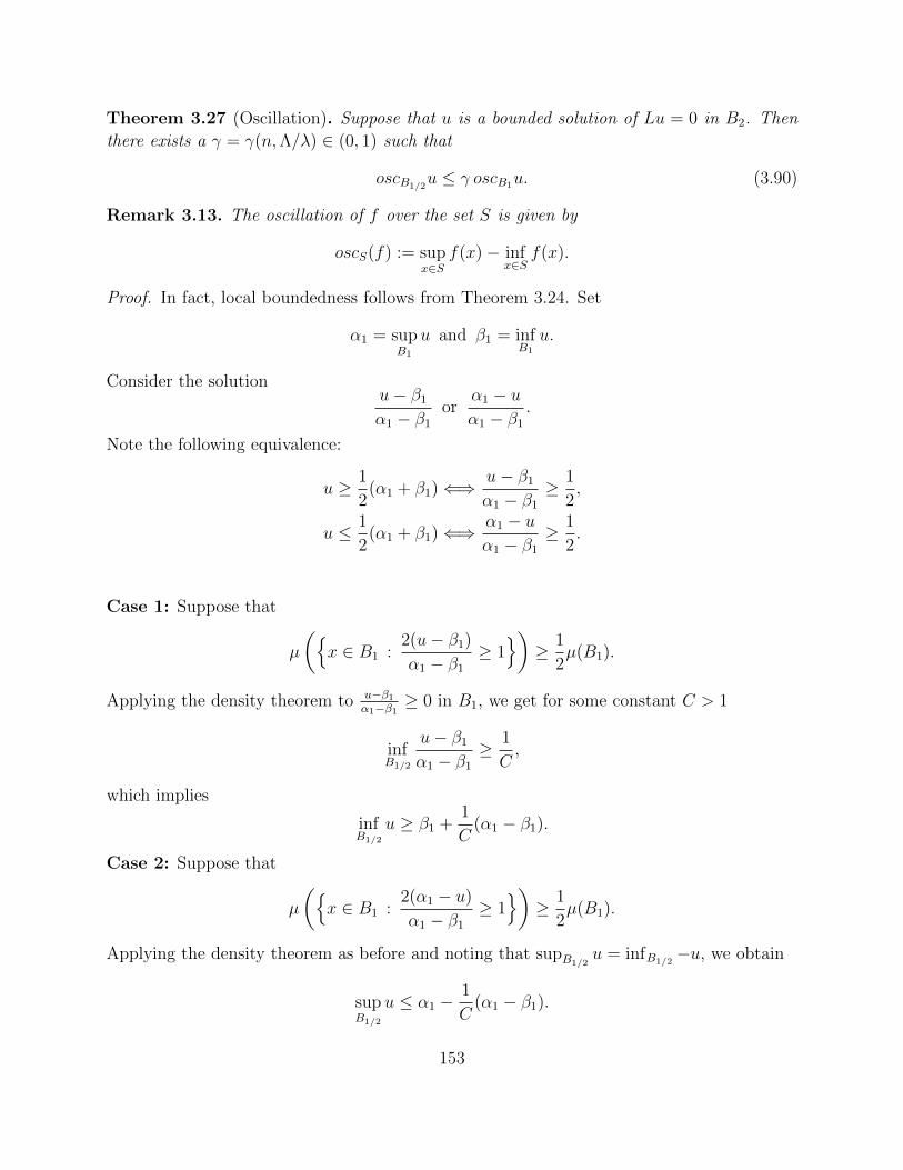
Theorem 3.27 (Oscillation). Suppose that u is a bounded solution of Lu = 0 in B2. Then
there exists a γ = γ(n,Λ/λ) ∈ (0, 1) such that
oscB1/2u ≤ γ oscB1u. (3.90)
Remark 3.13. The oscillation of f over the set S is given by
oscS(f) := supx∈S
f(x)− infx∈S
f(x).
Proof. In fact, local boundedness follows from Theorem 3.24. Set
α1 = supB1
u and β1 = infB1
u.
Consider the solutionu− β1
α1 − β1
orα1 − uα1 − β1
.
Note the following equivalence:
u ≥ 1
2(α1 + β1)⇐⇒ u− β1
α1 − β1
≥ 1
2,
u ≤ 1
2(α1 + β1)⇐⇒ α1 − u
α1 − β1
≥ 1
2.
Case 1: Suppose that
µ
({x ∈ B1 :
2(u− β1)
α1 − β1
≥ 1})≥ 1
2µ(B1).
Applying the density theorem to u−β1
α1−β1≥ 0 in B1, we get for some constant C > 1
infB1/2
u− β1
α1 − β1
≥ 1
C,
which implies
infB1/2
u ≥ β1 +1
C(α1 − β1).
Case 2: Suppose that
µ
({x ∈ B1 :
2(α1 − u)
α1 − β1
≥ 1})≥ 1
2µ(B1).
Applying the density theorem as before and noting that supB1/2u = infB1/2
−u, we obtain
supB1/2
u ≤ α1 −1
C(α1 − β1).
153

Now set
α2 = supB1/2
u and β2 = infB1/2
u,
and note that β2 ≥ β1 and α2 ≤ α1. In both cases, we have
α2 − β2 ≤(
1− 1
C
)(α1 − β1).
This is precisely the estimate (3.90) with γ = 1− 1/C ∈ (0, 1).
At last, we are now equipped to state and prove De Giorgi’s Holder regularity theorem.
Theorem 3.28 (De Giorgi). Suppose Lu = 0 weakly in B1. Then there holds
supB1/2
|u(x)|+ supx,y∈B1/2
|u(x)− u(y)||x− y|α
≤ C(n,Λ/λ)‖u‖L2(B1),
where α = α(n,Λ/λ) ∈ (0, 1).
Proof. The first part of the estimate follows from Theorem 3.24; that is,
supB1/2
|u(x)| ≤ C(n,Λ/λ)‖u‖L2(B1).
We prove the second part of the estimate. Fix any two distinct points x, y ∈ B1/2, set
r = |x− y| and let
ω(r) := oscBr(u) = supBr
u− infBru.
By Theorem 3.27 and rescaling, we obtain that
ω(r/2) ≤ γω(r).
Hence, Lemma 3.10 implies that
ω(r) ≤ Crαω(1/2) for all 0 < r ≤ 1/2,
where α = α(n,Λ/λ) is some number in (0, 1). By Theorem 3.24, we have that
ω(1/2) ≤ supB1/2
|u(x)| ≤ C‖u‖L2(B1).
Inserting this into the previous estimate yields
ω(r) ≤ Crα‖u‖L2(B1),
which further implies
supx,y∈B1/2
|u(x)− u(y)||x− y|α
≤ C(n,Λ/λ)‖u‖L2(B1).
This completes the proof.
154

3.7.5 Holder Regularity: the Weak Harnack Inequality
We now state and prove the weak Harnack inequality. As a result, we derive Moser’s Harnack
inequality as a special case, and we combine it with our previous local boundedness result to
give another proof of the interior Holder continuity of weak solutions. Then, we also examine
applications of the weak Harnack inequality to obtain a Liouville type theorem and a version
of the strong maximum principles for weak solutions.
For simplicity, we only consider elliptic equations without lower order terms. Suppose
U ⊂ Rn, aij ∈ L∞(U) satisfies
λ|ξ|2 ≤ aij(x)ξiξj ≤ Λ|ξ|2 for all x ∈ U and ξ ∈ Rn
for some positive constants λ and Λ.
Theorem 3.29 (Weak Harnack inequality). Let u ∈ H1(U) be a non-negative supersolution
in U , i.e.,
ˆU
aij(x)DiuDjϕdx ≥ˆU
fϕ dx for any non-negative ϕ ∈ H10 (U). (3.91)
Suppose f ∈ Lq(U) for some q > n/2. Then for any BR ⊂ U , there holds for any p ∈ (0, nn−2
)
and any 0 < θ < τ < 1,
infBθR
u+R2−nq ‖f‖Lq(BR) ≥ C
( 1
Rn
ˆBτR
up) 1p
where C = C(n, λ,Λ, p, q, θ, τ) is a positive constant.
The proof of the weak Harnack inequality and the result on the Holder continuity of
weak solutions will make use of the following result, which is a special case of the local
boundedness result of Theorem 3.24.
Theorem 3.30 (local boundedness). Let u ∈ H1(U) be a non-negative subsolution in U in
the following sense:
ˆU
aij(x)DiuDjϕdx ≤ˆU
fϕ dx for any non-negative ϕ ∈ H10 (U).
Suppose f ∈ Lq(U) for some q > n/2. Then there holds for any BR ⊂ U , any r ∈ (0, R),
and any p > 0,
supBr
u ≤ C{ 1
(R− r)n/p‖u+‖Lp(BR) +R2−n
q ‖f‖Lq(BR)
}where C = C(n, λ,Λ, p, q) is a positive constant.
155
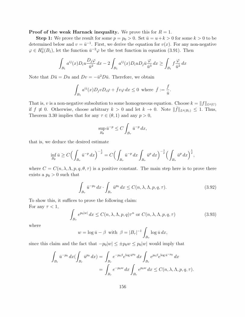
Proof of the weak Harnack inequality. We prove this for R = 1.
Step 1: We prove the result for some p = p0 > 0. Set u = u+k > 0 for some k > 0 to be
determined below and v = u−1. First, we derive the equation for v(x). For any non-negative
ϕ ∈ H10 (B1), let the function u−2ϕ be the test function in equation (3.91). Then
ˆB1
aij(x)DiuDjϕ
u2dx− 2
ˆB1
aij(x)DiuDjuϕ
u3dx ≥
ˆB1
fϕ
u2dx
Note that Du = Du and Dv = −u2Du. Therefore, we obtain
ˆB1
aij(x)DjvDiϕ+ fvϕ dx ≤ 0 where f :=f
u.
That is, v is a non-negative subsolution to some homogeneous equation. Choose k = ‖f‖Lq(U)
if f 6≡ 0. Otherwise, choose arbitrary k > 0 and let k → 0. Note ‖f‖Lq(B1) ≤ 1. Thus,
Theorem 3.30 implies that for any τ ∈ (θ, 1) and any p > 0,
supBθ
u−p ≤ C
ˆBτ
u−p dx,
that is, we deduce the desired estimate
infBθu ≥ C
(ˆBτ
u−p dx)− 1
p= C
( ˆBτ
u−p dx
ˆBτ
up dx)− 1
p(ˆ
Bτ
up dx) 1p,
where C = C(n, λ,Λ, p, q, θ, τ) is a positive constant. The main step here is to prove there
exists a p0 > 0 such that
ˆBτ
u−p0 dx ·ˆBτ
up0 dx ≤ C(n, λ,Λ, p, q, τ). (3.92)
To show this, it suffices to prove the following claim:
For any τ < 1, ˆBτ
ep0|w| dx ≤ C(n, λ,Λ, p, q)τn or C(n, λ,Λ, p, q, τ) (3.93)
where
w = log u− β with β = |Bτ |−1
ˆBτ
log u dx,
since this claim and the fact that −p0|w| ≤ ±p0w ≤ p0|w| would imply that
ˆBr
u−p0 dx(
ˆBr
up0 dx) =
ˆBr
e−p0βelog up0 dx
ˆBr
ep0βelog u−p0 dx
=
ˆBr
e−p0w dx
ˆBr
ep0w dx ≤ C(n, λ,Λ, p, q, τ).
156

To prove estimate (3.93), we notice that it follows directly from the John-Nirenberg lemma,
i.e., Lemma 3.2, provided that we show w ∈ BMO, i.e.,
1
rn
ˆBr
|w − wy,r| dx ≤ C.
We first derive the equation for w. As before, consider u−1ϕ to be the test function in (3.91)
and assume that ϕ is non-negative with ϕ ∈ L∞(B1) ∩H10 (B1). By direct calculations and
the fact that Dw = u−1Du, we get thatˆB1
aij(x)DiwDj(wϕ) dx ≤ˆB1
aij(x)DiwDjϕdx+
ˆB1
−fϕ dx (3.94)
for any non-negative ϕ ∈ L∞(B1) ∩ H10 (B1). Replace ϕ by ϕ2 in (3.94). Then Holder’s
inequality yieldsˆB1
|Dw|2ϕ2 dx ≤ C( ˆ
B1
|Dϕ|2 dx+
ˆB1
|f |ϕ2 dx). (3.95)
Furthermore, Holder’s inequality and the Sobolev embedding implyˆB1
|f |ϕ2 dx ≤ ‖f‖Ln/2(B1)‖ϕ‖2
L2nn−2 (B1)
≤ C(n, q)‖Dϕ‖2L2(B1).
Hence, ˆB1
|Dw|2ϕ2 dx ≤ C(n, q, λ,Λ)
ˆB1
|Dϕ|2 dx. (3.96)
Here, we can choose ϕ to be in C10(B1). Moreover, for any B2r(y) ⊂ B1, we can choose ϕ
with suppϕ ⊂ B2r(y), ϕ ≡ 1 in Br(y), and |Dϕ| ≤ 2r. Then
ˆBr(y)
|Dw|2 dx ≤ Crn−2.
Hence, Poincare’s inequality yields
1
rn
ˆBr(y)
|w − wy,r| dx ≤1
rn/2
(ˆBr(y)
|w − wy,r|2 dx) 1
2 ≤ 1
rn/2
(r2
ˆBr(y)
|Dw|2 dx) 1
2 ≤ C.
That is, w ∈ BMO and this proves the claim.
Step 2: We now verify the result for any p ∈ (0, nn−2
), but we only sketch the main steps
as it is similar to the proof of Theorem 3.24. It suffices to prove the following claim. Namely,
by the existence of p0 from Step 1, Moser’s iteration scheme yields, for any 0 < r1 < r2 < 1
and 0 < p2 < p1 <nn−2
,(ˆBr1
up1 dx) 1p1 ≤ C(n, q, λ,Λ, r1, r2, p1, p2)
( ˆBr2
up2 dx) 1p2 . (3.97)
157

To start, we take ϕ = u−β−1η2 for β ∈ (0, 1) as the test function in (3.91). Then, we can
establish thatˆB1
|Du|2u−β−1η2 dx ≤ C{ 1
β2
ˆB1
|Dη|2u1−β dx+1
β
ˆB1
|f |kη2u1−β dx
}.
Set γ = 1− β ∈ (0, 1) and w = uγ/2. Then we have
ˆ|Dw|2η2 dx ≤ C
(1− γ)α
ˆw2(|Dη|2 + η2) dx
or ˆ|D(wη)|2dx ≤ C
(1− γ)α
ˆw2(|Dη|2 + η2) dx
for some positive α > 0. By the Sobolev embedding and a proper choice of a cutoff function
with χ = n/(n− 2), we obtain for any γ ∈ (0, 1) and 0 < r < R < 1,( ˆBr
w2χ dx)1/χ
≤ C
(1− γ)α1
(R− r)2
ˆBR
w2 dx,
or (ˆBr
uγχ dx)1/γχ
≤( C
(1− γ)α1
(R− r)2
)1/γ(ˆBR
uγ dx)1/γ
≤(C(1 + γ)1+σ
R− r
)2/γ(ˆBR
uγ dx)1/γ
(3.98)
for some σ > 0. We may iterate this last estimate finitely-many times to get (3.97).
A special case of the weak Harnack inequality is Moser’s version.
Theorem 3.31 (Moser’s Harnack inequality). Let u ∈ H1(U) be a non-negative solution in
U , i.e., ˆU
aij(x)DiuDjϕdx =
ˆU
fϕ dx for any ϕ ∈ H10 (U).
Suppose f ∈ Lq(U) for some q > n/2. Then there holds for any BR ⊂ U ,
maxBR/2
u ≤ C(
minBR/2
u+R2−nq ‖f‖Lq(BR)
)where C = C(n, λ,Λ, q) is a positive constant.
The proof of Moser’s version of the Harnack inequality follows from the weak version and
Lemma 3.9.
158

Proof of Moser’s Harnack Inequality. Define Φ(p, r) by
Φ(p, r) :=(ˆ
Br
up dx)1/p
.
Then (3.98) implies the estimate
Φ(χγ, r) ≤(C(1 + γ)σ+1
R− r
)2/γ
Φ(γ,R). (3.99)
Set for m = 0, 1, 2, 3, . . . ,
γ = γm = χmp and rm = 1/2 + 2−(m+1).
Then, by iterating estimate (3.99), we get
Φ(χmγ, 1/2) ≤ (Cχ)2(1+σ)∑mχ−mΦ(p, 1).
By sending m −→∞ here and applying Lemma 3.9, we arrive at
supB1/2
u ≤ CΦ(p, 1).
The desired estimate follows from this and the weak Harnack inequality.
Now, our goal is to establish the Holder continuity of weak solutions using the local
boundedness result and Moser’s Harnack inequality.
Corollary 3.3 (Holder continuity). Let u ∈ H1(U) be a solution of the equation in U :ˆU
aij(x)DiuDjϕdx =
ˆU
fϕ dx for any ϕ ∈ H10 (U).
Suppose f ∈ Lq(U) for some q > n/2. Then u ∈ Cα(U) for some α ∈ (0, 1) depending only
on n, q, λ and Λ. Moreover, there holds for any BR ⊂ U
|u(x)− u(y)| ≤ C( |x− y|
R
)α{( 1
Rn
ˆBR
u2 dx) 1
2+R2−n
q ‖f‖Lq(BR)
}for any x, y ∈ BR/2 where C = C(n, λ,Λ, q) is a positive constant.
Proof. We prove the estimate for the case R = 1. Set for r ∈ (0, 1)
M(r) = maxBr
u and m(r) = minBr
u.
Then M(r) <∞ and m(r) > −∞. It suffices to prove for any r < 1/2,
ω(r) := M(r)−m(r) ≤ Crα{(ˆ
B1
u2 dx) 1
2+ ‖f‖Lq(B1)
}. (3.100)
159

Set δ = 2− n/q and apply Theorem 3.31 to M(r)− u ≥ 0 in Br to get
supBr/2
(M(r)− u) ≤ C{
infBr/2
(M(r)− u) + rδ‖f‖Lq(Br)}.
Combining this with the definitions of the supremum and infimum, we get
infBr/2
(M(r)− u) ≤ supBr/2
(M(r)− u)
≤ C{
infBr/2
(M(r)− u) + rδ‖f‖Lq(Br)}≤ C
{supBr/2
(M(r)− u) + rδ‖f‖Lq(Br)}.
Hence,
M(r)−m(r/2) ≤ C{
(M(r)−M(r/2)) + rδ‖f‖Lq(Br)}. (3.101)
Likewise, applying the same argument to u−m(r) ≥ 0 in Br, we get
M(r/2)−m(r) ≤ C{
(m(r/2)−m(r)) + rδ‖f‖Lq(Br)}. (3.102)
Adding (3.101) and (3.102) together yields
ω(r) + ω(r/2) ≤ C{
(ω(r)− ω(r/2)) + rδ‖f‖Lq(Br)}
or
ω(r/2) ≤ γω(r) + Crδ‖f‖Lq(Br)for some γ = (C − 1)/(C + 1) < 1.
Apply Lemma 3.10 with µ is chosen such that α = (1− µ) log γ/ log τ < µδ. Then
ω(ρ) ≤ Cρα{ω(1/2) + ‖f‖Lq(B1)} for any ρ ∈ (0, 1/2]. (3.103)
On the other hand, Theorem 3.30 implies
ω(1/2) ≤ C{( ˆ
B1
u2 dx) 1
2+ ‖f‖Lq(B1)
}and inserting this into (3.103) completes the proof of the corollary.
3.7.6 Further Applications of the Weak Harnack Inequality
A Liouville theorem
First, we point out an application of Lemma 3.10. Namely, we can derive the following
Liouville theorem.
160

Theorem 3.32. Suppose u ∈ H1(U) is a solution to the homogeneous equation in Rn:ˆRnaij(x)DiuDjϕdx = 0 for any ϕ ∈ H1
0 (Rn).
If u is bounded, then u is constant.
Proof. From the previous corollary, we showed that there exists a γ < 1 such that
ω(r) ≤ γω(2r).
By iteration, we obtain
ω(r) ≤ γkω(2kr)→ 0 as k →∞
since ω(2kr) ≤ C if u is bounded. Hence, for any r > 0,
ω(r) = 0.
Thus, u ≡ constant.
Maximum principles for weak solutions
An application of the weak Harnack inequality is the strong maximum principle adapted for
weak solutions. However, we introduce some necessary definitions and consider the weak
maximum principle for weak solutions. We say that u ∈ H1(U) satisfies u ≤ 0 on ∂U
if its positive part u+ = max{u, 0} belongs to H10 (U). Of course if u is continuous in a
neighborhood of ∂U then u satisfies u ≤ 0 on ∂U if the inequality holds in the classical
pointwise sense. Likewise, we say u ≥ 0 on ∂U if −u ≤ 0 on ∂U ; and u ≤ v ∈ H1(U) on ∂U
if u− v ≤ 0 on ∂U . As usual, we take
Lu = −Di(aij(x)Dju)
and solutions, supersolutions, and subsolutions associated with this elliptic operator are
understood in the distributional sense.
Theorem 3.33 (Weak Maximum Principle for Weak Solutions). Let u ∈ H1(U).
(a) If Lu ≤ 0 in U , then supU u ≤ sup∂U u+.
(b) If Lu ≥ 0 in U , then infU u ≥ inf∂U u−.
Proof. Since Lu ≤ 0 in U in the distribution sense, we writeˆU
aij(x)DjuDiv dx ≤ 0
for all non-negative v ∈ H10 (U). If we set ` = sup∂U u
+ and take v = max{u − `, 0}, then
v ∈ H10 (U), Dv = Du if u − ` > 0 and Dv = 0 if u − ` ≤ 0. We proceed by contradiction.
161

That is, assume v > 0 or u > ` in some subset B ⊂⊂ U with µ(B) > 0; otherwise, if v ≡ 0
then we would be done. Clearly, Dv = Du within B; but the positivity of (aij(x)) and the
uniform ellipticity condition imply thatˆB
|Dv|2 dx ≤ 0,
and we get that v, and therefore u, is constant in a subset of U with positive measure. At the
same time, a basic result guarantees Du = 0 a.e. in this subset and we deduce a contradiction.
This completes the proof for part (a). Part (b) follows along a similar argument; namely, we
can apply the previous proof to −Lu ≤ 0 and the fact that infD u = − supD(−u).
From this, we immediately deduce a uniqueness result.
Corollary 3.4. Let u ∈ H10 (U) satisfy Lu = 0 in U . Then u = 0 in U .
We are now ready to introduce the strong version of the maximum principle adapted for
weak solutions. Unlike the weak maximum principle above, we are only assuming the weak
solution belongs to H1(U). We do not assume the solution vanishes at the boundary in the
trace sense, i.e., it does not necessarily belong to H10 (U). The Harnack inequality plays an
essential role in its proof.
Theorem 3.34 (Strong Maximum Principle for Weak Solutions). Let U be a bounded and
open subset and let u ∈ H1(U) satisfy Lu ≤ 0 in U . Then, if for some ball B ⊂⊂ U we have
supBu = sup
Uu ≥ 0, (3.104)
the function u must be constant in U .
Proof. Denote B = BR(y) and without loss of generality, we can assume that B4R(y) ⊂ U .
Now let M = supU u and then apply the weak Harnack inequality (see Theorem 3.29) with
p = 1 to the supersolution v = M − u. Namely, we use the following dilated version of the
weak Harnack inequality with p = 1:
R−n‖v‖L1(B2R(y)) ≤ C infBR(y)
v.
Hence,
R−nˆB2R
(M − u) dx ≤ C infB
(M − u) = 0
and so u ≡ M in B2R. Therefore, supremum of u is attained for a larger ball in U . We can
then show u ≡M in U by a simple covering argument.
Remark 3.14. Likewise, we have an analogous result which states the solution to Lu ≥ 0
in U is constant whenever it attains an interior minimum.
162

CHAPTER 4
Viscosity Solutions and Fully Nonlinear Equations
4.1 Introduction
This chapter introduces a very weak concept of solution for second-order elliptic equations
called viscosity solutions. To simplify our presentation, the results given here are for equa-
tions involving linear elliptic operators without lower order terms, but they can certainly be
extended to fully nonlinear elliptic equations of the type
F (D2u, u, x) = f(x) in U,
where F : Rn×n × R× Rn is usually a monotone and convex mapping possibly nonlinear in
D2u and u. For a nice introductory treatment of this topic, we refer the reader to Caffarelli
and Cabre [3].
The advantage of considering the notion of viscosity solution is it allows us to consider
elliptic equations in non-divergence form, and it extends the notion of classical solutions.
Another advantage is that viscosity solutions are stable under local uniform convergence
in both u and F and because existence and uniqueness results for such solutions can be
obtained under far more general conditions. In fact, in the definition given below, notice
that we can make sense of such solutions without resorting to differentiating the equations
directly. This was a major obstacle in extending elliptic theory to equations having non-
divergence form, since the usual procedure of integrating by parts and treating equations
in the distribution sense was not generally possible, or the usual notions of solution was
not always guaranteed to exist in this context. Thus, finding a successful framework that
circumvents this obstacle was a tremendous breakthrough in the modern theory of elliptic
partial differential equations.
163

The results we establish below should be reminiscent of those for elliptic equations in
divergence form studied earlier, however, we obtain the results via perturbation methods
relying heavily on approximation and density arguments. More precisely, we shall give a
concise introduction, develop the Alexandroff maximum principle along with a Harnack
inequality for viscosity solutions. Then we use these to develop the interior Schauder and
W 2,p regularity estimates for viscosity solutions. Global versions of these regularity results
without proof are also provided at the end of the chapter.
Let U be a bounded and connected domain in Rn and (aij) is of class C(U) and satisfies
λ|ξ|2 ≤ aij(x)ξiξj ≤ Λ|ξ|2
for any x ∈ U and any ξ ∈ Rn. We consider the operator L in U defined by
Lu = −n∑
i,j=1
aij(x)Diju for u ∈ C2(U). (4.1)
Throughout, we shall assume that f belongs to C(U).
Definition 4.1. The function u ∈ C(U) is said to be a viscosity supersolution (respec-
tively viscosity subsolution) of the equation
Lu = f in U (4.2)
if for any x0 ∈ U and any function ϕ ∈ C2(U) such that u − ϕ has a local minimum
(respectively, local maximum) at x0 there holds
Lϕ(x0) ≥ f(x0) (respectively,Lϕ(x0) ≤ f(x0)).
The following definition of solution should be compared with the result of Theorem 1.10.
Definition 4.2. We say u ∈ C(U) is a viscosity solution of equation (4.1) if it is both a
viscosity subsolution and a viscosity supersolution.
Remark 4.1. By density, the C2 function ϕ in the above definitions may be replaced by
quadratic polynomials.
Next we look at the class of all solutions to all elliptic equations. First we make the
following important observation. Let e1, e2, . . . , en be the eigenvalues of the Hessian matrix
D2ϕ(x0) where ϕ is any C2 function at x0 ∈ U . We have the following chain of equivalent
estimates:n∑
i,j=1
aij(x0)Dijϕ(x0) ≤ 0⇐⇒n∑i=1
αiei ≤ 0 for αi ∈ [λ,Λ],
⇐⇒∑ei>0
αiei +∑ei<0
αiei ≤ 0,
⇐⇒∑ei>0
αiei ≤∑ei<0
αi(−ei),
164

where the last line implies
λ∑ei>0
αiei ≤ Λ∑ei<0
αi(−ei).
Namely, if u is a “supersolution,” then the positive eigenvalues of the Hessian matrix D2ϕ(x0)
are controlled by its negative eigenvalues. This motivates the following definition.
Definition 4.3. Suppose f ∈ C(U) and λ and Λ are two positive constants. We define
u ∈ C(U) to belong to S+(λ,Λ, f) if for any x0 ∈ U and any function ϕ ∈ C2(U) such that
u− ϕ has a local minimum at x0, there holds
λ∑
ei(x0)>0
ei(x0) + Λ∑ei<0
ei(x0) ≥ f(x0),
where e1(x0), e2(x0), . . . , en(x0) are eigenvalues of the Hessian matrix D2ϕ(x0).
Similarly, we define u ∈ C(U) to belong to S−(λ,Λ, f) if for any x0 ∈ U and any function
ϕ ∈ C2(U) such that u− ϕ has a local maximum at x0, there holds
Λ∑
ei(x0)>0
ei(x0) + λ∑ei<0
ei(x0) ≤ f(x0).
We denote S(λ,Λ, f) = S+(λ,Λ, f) ∩ S−(λ,Λ, f)
Notice that any viscosity supersolution of (4.2) belongs to the class S+(λ,Λ, f). In fact,
the class S+(λ,Λ, f) and S−(λ,Λ, f) also include solutions to fully nonlinear equations such
as the Pucci equations.
We say the matrix A = (aij) belongs to the class Aλ,Λ with any two constants λ,Λ > 0
if A is symmetric and
λ|ξ|2 ≤ aij(x)ξiξj ≤ Λ|ξ|2 for x ∈ U, ξ ∈ Rn
so that its eigenvalues belong to [λ,Λ].
Now, for any symmetric matrix M = (mij), we define the Pucci extremal operators:
M−(M) =M−(λ,Λ,M) = infA∈Aλ,Λ
aijmij,
M+(M) =M+(λ,Λ,M) = supA∈Aλ,Λ
aijmij.
Then Pucci’s equations are given by
M−(λ,Λ,M) = f,
M+(λ,Λ,M) = g,
165
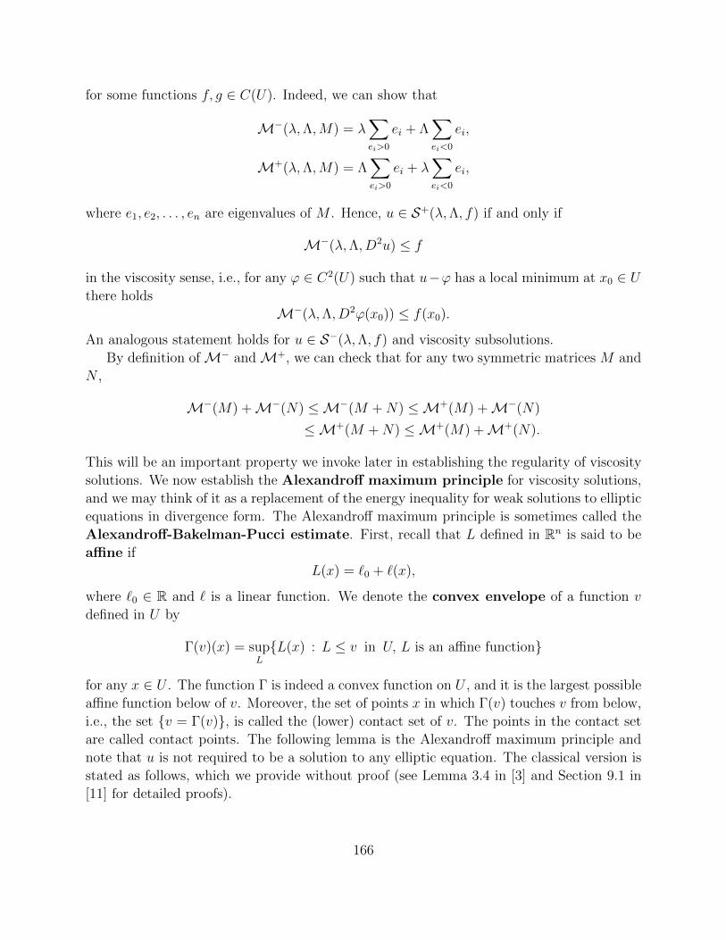
for some functions f, g ∈ C(U). Indeed, we can show that
M−(λ,Λ,M) = λ∑ei>0
ei + Λ∑ei<0
ei,
M+(λ,Λ,M) = Λ∑ei>0
ei + λ∑ei<0
ei,
where e1, e2, . . . , en are eigenvalues of M . Hence, u ∈ S+(λ,Λ, f) if and only if
M−(λ,Λ, D2u) ≤ f
in the viscosity sense, i.e., for any ϕ ∈ C2(U) such that u−ϕ has a local minimum at x0 ∈ Uthere holds
M−(λ,Λ, D2ϕ(x0)) ≤ f(x0).
An analogous statement holds for u ∈ S−(λ,Λ, f) and viscosity subsolutions.
By definition ofM− andM+, we can check that for any two symmetric matrices M and
N ,
M−(M) +M−(N) ≤M−(M +N) ≤M+(M) +M−(N)
≤M+(M +N) ≤M+(M) +M+(N).
This will be an important property we invoke later in establishing the regularity of viscosity
solutions. We now establish the Alexandroff maximum principle for viscosity solutions,
and we may think of it as a replacement of the energy inequality for weak solutions to elliptic
equations in divergence form. The Alexandroff maximum principle is sometimes called the
Alexandroff-Bakelman-Pucci estimate. First, recall that L defined in Rn is said to be
affine if
L(x) = `0 + `(x),
where `0 ∈ R and ` is a linear function. We denote the convex envelope of a function v
defined in U by
Γ(v)(x) = supL{L(x) : L ≤ v in U, L is an affine function}
for any x ∈ U . The function Γ is indeed a convex function on U , and it is the largest possible
affine function below of v. Moreover, the set of points x in which Γ(v) touches v from below,
i.e., the set {v = Γ(v)}, is called the (lower) contact set of v. The points in the contact set
are called contact points. The following lemma is the Alexandroff maximum principle and
note that u is not required to be a solution to any elliptic equation. The classical version is
stated as follows, which we provide without proof (see Lemma 3.4 in [3] and Section 9.1 in
[11] for detailed proofs).
166

Lemma 4.1. Suppose u is a C1,1 function in B1 with u ≥ 0 on ∂B1. Then
supB1
u− ≤ C(n)(ˆ
B1∩{u=Γu}det(D2u) dx
)1/n
,
where Γu is the convex envelope of −u− = min{u, 0}.
The version of this for viscosity solutions is the following, which we will prove with the
help of Lemma 4.1.
Theorem 4.1 (Alexandroff Maximum Principle). Suppose u belongs to S+(λ,Λ, f) in B1
with u ≥ 0 on ∂B1 for some f ∈ C(U). Then
supB1
u− ≤ C(n, λ,Λ)( ˆ
B1∩{u=Γu}(f+)n dx
)1/n
,
where Γu is the convex envelope of −u− = min{u, 0}.
Proof. The goal is to ultimately apply Lemma 4.1 to the convex envelope Γu(x). Namely,
we need to prove that Γu belongs to C1,1(B1) and at a contact point x0, we have that
f(x0) ≥ 0 (4.3)
and
L(x) ≤ Γu(x) ≤ L(x) + C(n, λ,Λ)(f(x0) + ε(x))|x− x0|2 (4.4)
for some affine function L and any x sufficiently close to x0 with ε(x) = o(1) as x −→ x0.
Once we prove this claim, clearly (4.4) implies that
det(D2Γu)(x) ≤ C(n, λ,Λ)f(x)n for a.e.x ∈ {u = Γu}.
So Lemma 4.1 applied to the function Γu implies the result. Therefore, it remains to prove
the claim.
Let x0 be a contact point, i.e., u(x0) = Γu(x0). Without loss of generality, assume x0 = 0.
We may also assume, after subtracting a supporting plane at x0 = 0 if necessary, that u ≥ 0
in B1 with u(0) = 0. Take h(x) = −ε|x|2/2 in B1. Clearly, u − h has a minimum at 0,
and note that the eigenvalues of D2h(0) is just −ε with multiplicity n. By definition of
S+(λ,Λ, f), we have that
−nΛε ≤ f(0).
We obtain (4.3) after sending ε −→ 0 in the preceding estimate.
Finally, to obtain estimate (4.4), we will prove
0 ≤ Γu(x) ≤ C(n, λ,Λ)(f(0) + ε(x))|x|2 for x ∈ B1,
where ε(x) = o(1) as x −→ 0.
167

We need to get an estimate for
Cr =1
r2maxBr
Γu
for small r > 0. By convexity, Γu attains its maximum in the closed ball Br at some point on
the boundary, say at (0, . . . , 0, r). Now the set {x ∈ B1 : Γu(x) ≤ Γu(0, . . . , 0, r)} is convex
and contains Br. Hence,
Γu(x′, r) ≥ Γu(0, . . . , 0, r) = Crr
2 for any x = (x′, r) ∈ B1.
Choose a positive number N to be specified at a later time. Set
Rr = {(x′, xn) : |x′| ≤ Nr, |xn| ≤ r}.
We construct a quadratic polynomial that touches u from below in Rr and curves upward
very steeply. Set, for some b > 0,
h(x) = (xn + r)2 − b|x′|2.
Then,
(a) for xn = −r, h ≤ 0;
(b) for |x′| = Nr, h ≤ (4− bN2)r2 ≤ 0 if we take b = 4/N2;
(c) for xn = r, h = 4r2 − b|x′|2 ≤ 4r2.
Therefore, if we take
h(x) =Cr4h(x) =
Cr4
((xn + r)2 − 4
N2|x′|2
),
and since Γu is the convex envelope of u, we have h ≤ Γu ≤ u on ∂Rr. Moreover, h(0) =
Crr2/4 > 0 = Γu(0) = u(0). Then, after lowering h if necessary, we deduce that u− h has a
local minimum in the interior of Rr. It is easily checked that the eigenvalues of D2h are
Cr/2,−2Cr/N2, . . . ,−2Cr/N
2.
Hence, by definition of S+(λ,Λ, f), we have that
λCr2− 2Λ(n− 1)
CrN2≤ max
Rrf.
We can now choose N suitably large, which depends only on n, λ and Λ, so that
2Λ(n− 1)/N2 ≤ λ/4.
168

Thus, we obtain
Cr ≤4
λmaxRr
f ; that is, maxBr
Γu ≤4
λr2 max
Rrf.
Hence,
Γu(x) ≤ maxBr
Γu ≤4
λε(r)r2,
where ε(|x|) = ε(r) = maxRr f = o(1). This completes the proof.
Finally, we end this section with a basic result as a consequence of the Calderon-Zygmund
decompostion. We will need this result when establishing the Harnack inequality and the
regularity theory for viscosity solutions. Here we work in dyadic cubes rather than balls.
Q denotes such a dyadic cube after refinement of a given Euclidean domain. We often use
Q`(x0) to denote a dyadic cube centered at x0 ∈ Rn with side length `. Sometimes we omit
x0 if x0 = 0, i.e., Q`(0) = Q`.
Lemma 4.2. Suppse measurable sets A ⊂ B ⊂ Q1 have the following properties.
(a) |A| < δ for some δ ∈ (0, 1);
(b) for any dyadic cube Q, |A ∩Q| ≥ δ|Q| implies Q ⊂ B for the predecessor Q of Q.
Then |A| ≤ δ|B|.
4.2 A Harnack Inequality
Theorem 4.2 (Harnack inequality). Suppose u belongs to S(λ,Λ, f) in B1 with u ≥ 0 in
B1 for some f ∈ C(B1). Then
supB1/2
u ≤ C(
infB1/2
u+ ‖f‖Ln(B1)
)(4.5)
where C is a positive constant depending only on n, λ and Λ.
As we have encountered already, Harnack type inequalities imply the interior Holder
regularity of solutions. Thus, we have the following result whose proof we omit but follows
similarly to that of Corollary 3.3.
Corollary 4.1. Suppose u belongs to S(λ,Λ, f) in B1 for some f ∈ C(B1). Then u ∈ Cα(B1)
for some α ∈ (0, 1) depending only on n, λ, and Λ. In particular,
|u(x)− u(y)| ≤ C|x− y|α(
supB1
|u|+ ‖f‖Ln(B1)
)for any x, y ∈ B1/2.
The main ingredient in proving the Harnack inequality is the following result.
169

Proposition 4.1. Suppose u belongs to S(λ,Λ, f) in Q4√n with u ≥ 0 in Q4
√n for some
f ∈ C(Q4√n). Then there exist two positive constants ε0 and C, depending only on n, λ, and
Λ, such that if
infQ1/4
u ≤ 1 and ‖f‖Ln(Q4√n) ≤ ε0,
then
supQ1/4
u ≤ C.
To see how Theorem 4.2 follows from this, consider the function
uδ =u
infQ1/4u+ δ + ε−1
0 ‖f‖Ln(Q4√n)
(δ > 0),
provided that u ∈ S(λ,Λ, f) in Q4√n with u ≥ 0 in Q4
√n. Applying Proposition 4.1 to uδ
then sending δ −→ 0, we get
supQ1/4
u ≤ C( infQ1/4
u+ ‖f‖Ln(Q4√n)).
Then estimate (4.5) follows from a standard covering argument.
Lemma 4.3. Suppose u belongs to S+(λ,Λ, f) in B2√n for some f ∈ C(B2
√n). Then there
exist constants ε0 > 0, µ ∈ (0, 1), and M > 1, depending only on n, λ, and Λ, such that if
u ≥ 0 in B2√n, inf
Q3
u ≤ 1 and ‖f‖Ln(B2√n) ≤ ε0, (4.6)
then
|{u ≤M} ∩Q1| > µ.
Proof. The idea here to localize where the contact set occurs by choosing suitable functions.
Namely, we construct a function g that is “very concave” outside Q1 so that if we “correct”
u by g, the contact set is in Q1. First note that B1/4 ⊂ B1/2 ⊂ Q1 ⊂ Q3 ⊂ B2√n. Define g
in B2√n by
g(x) = −M(1− |x|2/4n)β
for some β > 0 to be specified later and some M > 0. We choose M with respect to β so
that
g ≡ 0 on ∂B2√n, and g ≤ −2 in Q3. (4.7)
Set w = u + g in B2√n. We shall prove that w, in particular g, belongs to S+(λ,Λ, f) in
B2√n\Q1 provided we choose β large enough. Suppose ϕ is a quadratic polynomial such that
w − ϕ has a local minimum at x0 ∈ B2√n. Then u− (ϕ− g) has a local minimum at x0 as
well. By definitions of S+(λ,Λ, f) and the Pucci extremal operator M−,
M−(λ,Λ, D2ϕ(x0)−D2g(x0)) ≤ f(x0),
170

or
M−(λ,Λ, D2ϕ(x0)) +M−(λ,Λ,−D2g(x0)) ≤ f(x0).
Therefore, to show g belongs to S+(λ,Λ, f) inB2√n\Q1, it remains to showM−(λ,Λ,−D2g(x0))
is non-negative. Well, the Hessian matrix of g is given by
Dijg(x) = (Mβ/2n)(1− |x|2/4n)β−1δij − [Mβ(β − 1)/(2n)2](1− |x|2/4n)β−2xixj.
Choose x = (|x|, 0, 0, . . . , 0), then the eigenvalues of −D2g(x) are given by
e+ = (Mβ/2n)(1− |x|2/4n)β−2((2β − 1)|x|2/4n− 1) with multiplicity 1,
e− = − (Mβ/2n)(1− |x|2/4n)β−2 with multiplicity n− 1.
Now choose β > 0 large enough so that e+ > 0 and e− < 0 for |x| ≥ 1/4. Thus, for |x| ≥ 1/4,
we have
M−(λ,Λ,−D2g(x)) = λe+(x) + (n− 1)Λe−(x)
=Mβ
2n(1− |x|2/4n)β−2
[λ(2β − 1
4n|x|2 − 1
)− (n− 1)Λ(1− |x|2/4n)
]≥ 0.
In fact, we have actually proved that
w ∈ S+(λ,Λ, f + η) in B2√n
for some η ∈ C∞0 (Q1) and supp(η) ⊆ [0, C(nλ,Λ)]. We may apply the Alexandroff maximum
principle (Theorem 4.1) to w in B2√n. Also note that infQ3 w ≤ −1 and w ≥ 0 on ∂B2
√n
due to (4.6) and (4.7). Thus,
1 ≤ C( ˆ
B2√n∩{w=Γw}
(|f |+ η)n dx)1/n
≤ C‖f‖Ln(B2√n) + C|{w = Γw} ∩Q1|1/n.
Choosing ε0 small enough, we get
(1/2) ≤ C|{w = Γw} ∩Q1|1/n ≤ C|{u ≤M} ∩Q1|1/n
since w(x) = Γw(x) implies w(x) ≤ 0 and thus u(x) ≤ −g(x) ≤ M . This completes the
proof.
Next we derive the power decay property of the distribution function of u.
171

Lemma 4.4. Let u belong to S+(λ,Λ, f) in B2√n for some f ∈ C(B2
√n). Then there exist
positive constants ε0, ε and C, depending only on n, λ, and Λ, such that if
u ≥ 0 in B2√n, inf
Q3
u ≤ 1 and ‖f‖Ln(B2√n) ≤ ε0, (4.8)
then
|{u ≥ t} ∩Q1| ≤ Ct−ε for t > 0.
Proof. Under the assumptions (4.8), we claim
|{u > Mk} ∩Q1| ≤ (1− µ)k for k = 1, 2, . . . , (4.9)
where M and µ are the same parameters from Lemma 4.3. We proceed by induction. Indeed,
for k = 1, (4.9) is just Lemma 4.3. So assume (4.9) holds for k− 1. Set A = {u > Mk}∩Q1
and B = {u > Mk−1} ∩Q1. We claim that
|A| ≤ (1− µ)|B| (4.10)
We do so by using Lemma 4.2. Clearly, A ⊂ B ⊂ Q1 and |A| ≤ |{u > M} ∩Q1| ≤ 1− µ by
Lemma 4.3. We claim that if Q = Qr(x0) is a cube in Q1 such that
|A ∩B| > (1− µ)|Q|, (4.11)
then Q ∩ Q1 ⊂ B for Q = Q3r(x0). We prove this by contradiction. Consider the transfor-
mation x = x0 + ry for y ∈ Q1 and x ∈ Q = Qr(x0), and the function
u(y) = M−(k−1)u(x).
Then u ≥ 0 in B2√n and infQ3 u ≤ 1. It is easy to check that u ∈ S+(λ,Λ, f) in B2
√n with
‖f‖Ln(B2√n) ≤ ε0. In fact,
f(y) =r2
Mk−1f(x) for y ∈ B2
√n.
Hence,
‖f‖Ln(B2√n)≤ r
Mk−1‖f‖Ln(B2
√n)≤ ‖f‖Ln(B2
√n)≤ ε0.
Therefore, u satisfies (4.8). Thus, Lemma 4.3 applied to u implies
µ < |{u(y) ≤M} ∩Q1| = r−n|{u(x) ≤Mk} ∩Q|.
Hence, |Q ∩ Ac| > µ|Q|, but this contradicts with (4.11). Applying Lemma 4.2 yields
(4.10).
172

Proof of Proposition 4.1. We show there exist two constants θ > 1 and M0 � 1, depending
only on n, λ, and Λ, such that if u(x0) = P > M0 for some x0 ∈ B1/4 there exists a sequence
{xk} ⊂ B1/2 such that
u(xk) ≥ θkP for k = 0, 1, 2, . . . .
This contradicts with the boundedness of u and thus supB1/4u ≤M0.
Suppose u(x0) = P > M0 for some x0 ∈ B1/4. We will determine M0 and θ in the process.
Consider a cube Qr(x0) centered at x0 with side length r, which will be specified below. We
want to find a point x1 ∈ Q4√nr(x0) such that u(x1) ≥ θP . To do so, we choose r such that
{u > P/2} covers less than half of Qr(x0). This can be done using the power decay of the
distribution function of u (see Lemma 4.4). Namely, since infQ3 u ≤ infQ1/4u ≤ 1, Lemma
4.4 implies
|{u > P/2} ∩Q1| ≤ C(P/2)−ε.
We choose r such that rn/2 ≥ C(P/2)−ε and r ≤ 1/4. Hence, we have, for such r, Qr(x0) ⊂Q1 and
1
|Qr(x0)||{u > P/2} ∩Qr(x0)| ≤ 1/2. (4.12)
Next we show that for θ > 1, with θ − 1 small, u ≥ θP at some point in Q4√nr(x0). We
proceed by contradiction. That is, assume u ≤ θP in Q4√nr(x0). Consider the transformation
x = r0 + ry for Q4√n and x ∈ Q4
√nr(x0)
and the function
u(y) =θP − u(x)
(θ − 1)P.
Clearly, u ≥ 0 in B2√n and u(0) = 1, and thus infQ3 u ≤ 1. It follows that u belongs to
S+(λ,Λ, f) in B2√n with ‖f‖Ln(B2
√n) ≤ ε0. Indeed, we have
f(y) = − r2
(θ − 1)Pf(x) for y ∈ B2
√n
and so
‖f‖Ln(B2√n) ≤
r
(θ − 1)P‖f‖Ln(B2
√n) ≤ ε0
provided we choose P so that r ≤ (θ − 1)P . Applying Lemma 4.3 to u and noting that
u(x) ≤ P/2 ⇐⇒ u(y) ≥ (θ − 1/2)/(θ − 1)� 1 provided that θ is close to 1, we get
1
|Qr(x0)||{u ≤ P/2} ∩Qr(x0)| = |u ≥ (θ − 1/2)/(θ − 1)} ∩Q1|
≤ C((θ − 1/2)/(θ − 1))−ε < 1/2.
This contradicts with (4.12). Hence, we deduce the existence of a θ = θ(n, λ,Λ) > 1 such
that if
u(x0) = P for some x0 ∈ B1/4,
173

then
u(x1) ≥ θP for some x1 ∈ Q4√nr(x0) ⊂ B2nr(x0)
provided that
C(n, λ,Λ)P−ε/n ≤ r ≤ (θ − 1)P.
Specifically, we need to choose P such that P ≥ (C/(θ−1))n/(n+ε) and then take r = CP−ε/n.
Iterating the previous result yields a sequence {xk} such that of for any k = 1, 2, 3, . . . ,
u(xk) ≥ θkP for some xk ∈ B2nrk(xk−1)
where rk = C(θk−1P )−ε/n = Cθ−(k−1)ε/nP−ε/n.
To ensure {xk} ⊂ B1/2, we take∑
2nrk < 1/4. Hence, we choose M0 so that
Mε/n0 ≥ 8nC
∞∑k=1
θ−(k−1)ε/n and M0 ≥( C
θ − 1
)n/(n+ε)
,
and choose P > M0. This completes the proof.
4.3 Schauder Estimates
In this section, we prove the Schauder estimates for viscosity solutions. Throughout this
section, we always assume that aij(x) ∈ C(B1) satisfies
λ|ξ|2 ≤ aij(x)ξiξj ≤ Λ|ξ|2
for any x ∈ B1 and any ξ ∈ Rn.
We shall need the following approximation result. Namely, it states that if the coefficient
matrix (aij(x)) is a “close” perturbation of the constant matrix (aij(0)) and thus is “close”
to the identity matrix by the uniform ellipticity assumption, then the viscosity solution u is
“close” to a solution of a Poisson equation at least locally.
Lemma 4.5. Suppose u ∈ C(B1) is a viscosity solution of
aij(x)Diju = f in B1
with |u| ≤ 1 in B1. Assume for some ε ∈ (0, 1/16),
‖aij − aij(0)‖Ln(B3/4) ≤ ε.
Then there exists a function h ∈ C(B3/4) with aij(0)Dijh = 0 in B3/4 and |h| ≤ 1 in B3/4
for which
‖u− h‖L∞(B1/2) ≤ C(εγ + ‖f‖Ln(B1))
where C > 0 is a constant and γ ∈ (0, 1) both depending only on n, λ, and Λ.
174

Proof. We can certainly solve for such a harmonic function h ∈ C(B3/4) ∩ C∞(B3/4) where
aij(0)Dijh = 0 in B3/4 and h = u on ∂B3/4. The maximum principle ensures |h| ≤ 1 in
B3/4 and note that u belongs to S(λ,Λ, f) in B1. Corollary 4.1 implies u ∈ Cα(B3/4) for
some α = α(n, λ,Λ) ∈ (0, 1). Thus, from the global Schauder regularity theory for harmonic
functions, the basic estimate
‖u‖Cα(B3/4) ≤ C(n, λ,Λ)(1 + ‖f‖Ln(B1))
implies
‖h‖Cα/2(B3/4) ≤ C‖u‖Cα(B3/4) ≤ C(n, λ,Λ)(1 + ‖f‖Ln(B1)).
Since u− h = 0 on ∂B3/4, we get for δ ∈ (0, 1/4),
‖u− h‖L∞(∂B3/4−δ) ≤ Cδα/2(1 + ‖f‖Ln(B1)). (4.13)
We claim that
‖D2h‖L∞(∂B3/4−δ) ≤ Cδα/2−2(1 + ‖f‖Ln(B1)). (4.14)
In fact, for any x0 ∈ B3/4−δ, applying interior C2 estimates on h − h(x1) in Bδ(x0) ⊂ B3/4
for some x1 ∈ ∂Bδ(x0) yields
|D2h(x0)| ≤ Cδ−2 supBδ(x0)
|h− h(x1)| ≤ Cδ−2δα/2(1 + ‖f‖Ln(B1)).
Note that u− h is a viscosity solution of
aij(x)Dij(u− h) = f(x)− (aij(x)− aij(0))Dijh := F in B3/4.
So by the Alexandroff maximum principle and (4.13)-(4.14),
‖u− h‖L∞(B3/4−δ) ≤ ‖u− h‖L∞(B3/4−δ) + C‖F‖Ln(B3/4−δ)
≤ ‖u− h‖L∞(B3/4−δ) + C‖D2‖L∞(B3/4−δ)‖aij − aij(0)‖Ln(B3/4) + C‖f‖Ln(B1)
≤ C(δα/2 + δα/2−2ε)(1 + ‖f‖Ln(B1)) + C‖f‖Ln(B1).
The proof is complete once we take δ =√ε and then γ = α/4.
Definition 4.4. A function g is Holder continuous at 0 with exponent α in the Ln sense if
[g]CαLn (0) = sup0≤r≤1
1
rα
( 1
|Br|
ˆBr
|g(x)− g(0)|n dx)1/n
<∞.
Theorem 4.3 (Schauder estimates). Suppose u ∈ C(B1) is a viscosity solution of
aij(x)Diju = f in B1.
175

Assume (aij) is Holder continous at 0 with exponent α in the Ln sense for some α ∈ (0, 1). If
f is Holder continuous at 0 with exponent α in the Ln sense, then u is C2,α at 0. Moreover,
there exists a polynomial P of degree 2 such that
|u− P |L∞(Br(0)) ≤ C∗r2+α for any r ∈ (0, 1),
|P (0)|+ |DP (0)|+ |D2P (0)| ≤ C∗,
C∗ ≤ C(‖u‖L∞(B1) + |f(0)|+ [f ]CαLn (0)),
where C > 0 is a constant depending only on n, λ,Λ, α and [aij]CαLn (0).
Proof. We organize the proof into two steps.
Step 1: Preparations We assume f(0) = 0 otherwise we may consider v = u−bijxixjf(0)/2
for some constant matrix (bij) such that aij(0)bij = 1. By scaling, we also assume that
[aij]CαLn (0) is small. Next, by considering for δ > 0,
u
‖u‖L∞(B1) + δ−1[f ]CαLn (0),
we may also assume ‖u‖L∞(B1) ≤ 1 and [f ]CαLn (0) ≤ δ.
Step 2: Suppose u ∈ C(B1) is a viscosity solution of
aij(x)Diju = f in B1
with
‖u‖L∞(B1) ≤ 1, [aij]CαLn (0) ≤ δ
and ( 1
|Br|
ˆBr
|f |n dx)1/n
≤ δrα for any r ∈ (0, 1).
We claim there exists a constant δ > 0, depending only on n, λ,Λ, and α and a polynomial
P of degree 2 with
‖u− P‖L∞(Br) ≤ Cr2+α for any r ∈ (0, 1), (4.15)
and
|P (0)|+ |DP (0)|+ |D2P (0)| ≤ C(n, λ,Λ, α). (4.16)
First, we show there exist µ ∈ (0, 1), depending only on n, λ,Λ, and α, and a sequence
of polynomials of degree 2,
Pk(x) = ak + bk · x+ (1/2)xTCkx,
such that for any k = 0, 1, 2, . . . ,
aij(0)DijPk = 0, ‖u− Pk‖L∞(Bµk
) ≤ µk(2+α), (4.17)
176

and
|ak − ak−1|+ µk−1|bk − bk−1|+ µ2(k−1)|Ck − Ck−1| ≤ Cµ(k−1)(2+α). (4.18)
Note that P0, P−1 ≡ 0 and C is a constant depending only on n, λ,Λ, and α.
Obviously, the theorem follows from (4.17)-(4.18) since ak, bk and Ck converge to some
a, b and C, and the limiting polynomial,
P (x) = a+ b · x+ (1/2)xTCx,
satisfies
|Pk(x)− P (x)| ≤ C(|x|2µαk + |x|µ(α+1)k + µ(α+2)k) ≤ Cµ(2+α)k
for any |x| ≤ µk. Hence, for |x| ≤ µk,
|u(x)− P (x)| ≤ |u(x)− Pk(x)|+ |Pk(x)− P (x)| ≤ Cµ(2+α)k,
which implies
|u(x)− P (x)| ≤ C|x|2+α for any x ∈ B1.
Therefore, it only remains to prove (4.17) and (4.18), and we do so by induction. The initial
step k = 0 is clearly true. Assume both estimates hold for k = 0, 1, . . . , `. We prove the next
step k = `+ 1 holds. Consider the function
u(y) =1
µ`(2+α)(u− P`)(µ`y) for y ∈ B1.
Then u belongs to C(B1) and is a viscosity solution of
aij(x)Diju = f in B1
where
aij(y) = µ−`αaij(µ`y),
and
f(y) = µ−`α(f(µ`y)− aij(µ`y)DijPk).
We want to apply Lemma 4.16. So we check that
‖aij − aij(0)‖Ln(B1) ≤ µ−`α‖aij − aij(0)‖Ln(Bµ`
) ≤ [aij]αLn(0) ≤ δ,
and
‖f‖Ln(B1) ≤ µ−`α‖f‖Ln(Bµ`
) + µ−`α sup |D2P`|‖aij − aij(0)‖Ln(Bµ`
) ≤ δ + Cδ
where we used
|D2P`| ≤∑k=1
|D2Pk −D2Pk−1| ≤∑k=1
µ(k−1)α ≤ C.
177
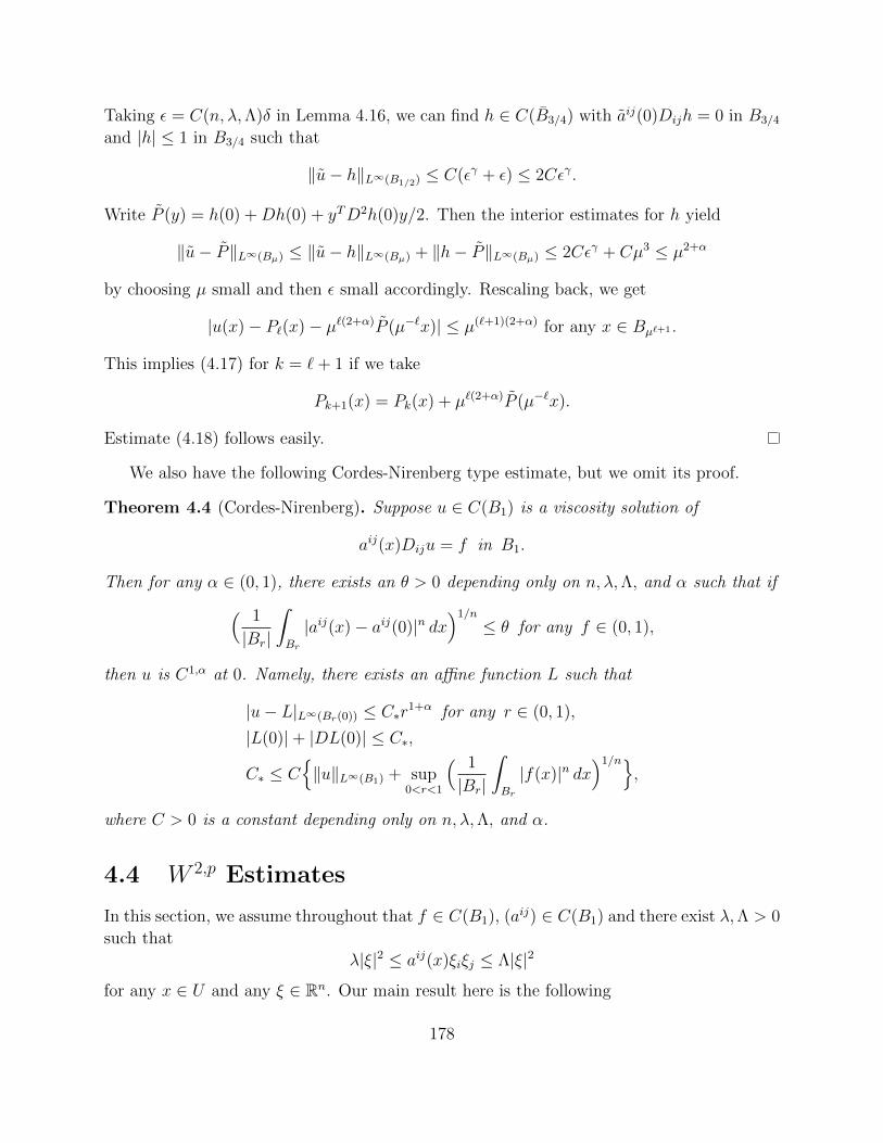
Taking ε = C(n, λ,Λ)δ in Lemma 4.16, we can find h ∈ C(B3/4) with aij(0)Dijh = 0 in B3/4
and |h| ≤ 1 in B3/4 such that
‖u− h‖L∞(B1/2) ≤ C(εγ + ε) ≤ 2Cεγ.
Write P (y) = h(0) +Dh(0) + yTD2h(0)y/2. Then the interior estimates for h yield
‖u− P‖L∞(Bµ) ≤ ‖u− h‖L∞(Bµ) + ‖h− P‖L∞(Bµ) ≤ 2Cεγ + Cµ3 ≤ µ2+α
by choosing µ small and then ε small accordingly. Rescaling back, we get
|u(x)− P`(x)− µ`(2+α)P (µ−`x)| ≤ µ(`+1)(2+α) for any x ∈ Bµ`+1 .
This implies (4.17) for k = `+ 1 if we take
Pk+1(x) = Pk(x) + µ`(2+α)P (µ−`x).
Estimate (4.18) follows easily.
We also have the following Cordes-Nirenberg type estimate, but we omit its proof.
Theorem 4.4 (Cordes-Nirenberg). Suppose u ∈ C(B1) is a viscosity solution of
aij(x)Diju = f in B1.
Then for any α ∈ (0, 1), there exists an θ > 0 depending only on n, λ,Λ, and α such that if( 1
|Br|
ˆBr
|aij(x)− aij(0)|n dx)1/n
≤ θ for any f ∈ (0, 1),
then u is C1,α at 0. Namely, there exists an affine function L such that
|u− L|L∞(Br(0)) ≤ C∗r1+α for any r ∈ (0, 1),
|L(0)|+ |DL(0)| ≤ C∗,
C∗ ≤ C{‖u‖L∞(B1) + sup
0<r<1
( 1
|Br|
ˆBr
|f(x)|n dx)1/n}
,
where C > 0 is a constant depending only on n, λ,Λ, and α.
4.4 W 2,p Estimates
In this section, we assume throughout that f ∈ C(B1), (aij) ∈ C(B1) and there exist λ,Λ > 0
such that
λ|ξ|2 ≤ aij(x)ξiξj ≤ Λ|ξ|2
for any x ∈ U and any ξ ∈ Rn. Our main result here is the following
178

Theorem 4.5. Suppose u ∈ C(B1) is a viscosity solution of
aij(x)Diju = f in B1.
For any p ∈ (n,∞), there exists an ε > 0 depending only on n, λ,Λ, and p such that if( 1
|Br(x0)|
ˆBr(x0)
|aij(x)− aij(x0)|n dx)1/n
≤ ε for any Br(x0) ⊂ B1,
then u ∈ W 2,ploc (B1). Moreover,
‖u‖W 2,p(B1/2) ≤ C(‖u‖L∞(B1) + ‖f‖Lp(B1)),
where C > 0 is a constant depending only on n, λ,Λ, and p.
As before, it suffices to prove the following.
Theorem 4.6. Suppose u ∈ C(B8√n) is a viscosity solution of
aij(x)Diju = f in B8√n.
For any p ∈ (n,∞), there exist ε > 0 and C > 0 depending only on n, λ,Λ, and p such that
if
‖u‖L∞(B8√n) ≤ 1 and ‖f‖Lp(B8
√n) ≤ ε
and if ( 1
|Br(x0)|
ˆBr(x0)
|aij(x)− aij(x0)|n dx)1/n
≤ ε for any Br(x0) ⊂ B8√n,
then u ∈ W 2,p(B1) and ‖u‖W 2,p(B1) ≤ C.
179

CHAPTER 5
The Method of Moving Planes and Its Variants
In this chapter, we introduce a powerful tool used to study the properties of solutions for
semilinear elliptic equations. The method is called the method of moving planes and it
originated from Alexandroff in his study of embedded constant mean curvature surfaces.
It was further developed in the works of Serrin [22] and Gidas, Ni and Nirenberg [10] and
later adapted to many other problems involving differential and integral equations (see [5]
and the references therein). We will focus on applying this method to obtain symmetry
and monotonicity results for positive solutions of the Lane-Emden equation and we shall
essentially adopt the framework of Chen and Li [4].
Consider the following semilinear elliptic problem
−∆u = up, x ∈ Rn, n ≥ 3. (5.1)
Our goal is to prove the following main result.
Theorem 5.1. For p = (n+ 2)/(n−2), every positive C2 solution of equation (5.1) must be
radially symmetric and monotone decreasing about some point, and thus assumes the form
u(x) =[n(n− 2)λ2]
n−24
(λ2 + |x− x0|2)n−2
2
for some λ > 0 and x0 ∈ Rn.
For 1 < p < (n+2)/(n−2), the only non-negative C2 solution of equation (5.1) is the trivial
one, u ≡ 0.
5.1 Preliminaries
We first start by introducing some necessary tools for the method of moving planes. Namely,
we introduce the Kelvin transform and various comparison theorems, i.e., maximum princi-
180

ples, for elliptic problems on unbounded domains. First, the Kelvin transform of the function
u, which we denote by u, is given by
u(x) =1
|x|n−2u( x
|x|2).
Then, if u is a solution of equation (5.1), then u is a solution of
−∆u = |x|p(n−2)−(n+2)up, x ∈ Rn\{0}. (5.2)
Now we introduce the maximum principles based on comparisons, which are the essential
ingredients in the method of moving planes.
Theorem 5.2. Assume that U is a bounded domain. Let φ be a positive function on U
satisfying
−∆φ+ λ(x)φ ≥ 0. (5.3)
Assume that u is a solution of{−∆u+ c(x)u ≥ 0 in U,
u ≥ 0 on ∂U.(5.4)
If
c(x) > λ(x) for all x ∈ U, (5.5)
then
u ≥ 0 in U.
If U is unbounded, then the result remains true provided that the following additional
condition is assumed:
lim inf|x|−→∞
u(x)
φ(x)≥ 0. (5.6)
Proof. We proceed by contradiction. Let v(x) = u(x)/φ(x) and assume that u < 0 at some
point in U . Thus, v < 0 at that same point, since φ is positive in U . Let x0 ∈ U be the
minimum of v and by a simple calculation, we obtain that
−∆v = 2Dv · Dφφ
+1
φ(−∆u+
∆φ
φu). (5.7)
However, since x0 is a minimum of v, we have that
−∆v(x0) ≤ 0 (5.8)
and
Dv(x0) = 0. (5.9)
181

But from (5.3)–(5.5) and since u(x0) < 0, we have that
−∆u(x0) +∆φ
φ(x0)u(x0) ≥ −∆u(x0) + λ(x0)u(x0) > −∆u(x0) + c(x0)u(x0) ≥ 0.
By inserting this into (5.7) and using (5.9), we get that −∆v(x0) > 0, but this contradicts
with (5.8). This completes the proof. In the case that U is unbounded, the same arguments
apply since the additional assumption (5.6) guarantees that the minimum of v does not leak
away to infinity.
Remark 5.1. As illustrated in the proof, conditions (5.3) and (5.5) are required only at the
points where v attains its minimum or at points where u is negative.
In our application of the above theorem, we will consider two cases:
(a) U is a “narrow” region,
(b) the coefficient c(x) has sufficient decay at infinity.
First, we examine when U is a narrow region; namely, let us consider the narrow strip with
width ` > 0, i.e.,
U = {x ∈ Rn | 0 < x1 < `}.We can take ϕ(x) = sin((x1 + ε)/`) so that −∆ϕ = (1/`)2ϕ. Thus, λ(x) = −(1/`)2, which
can be “very negative” if ` is suitably small.
Corollary 5.1 (Narrow region). If u satisfies (5.4) with bounded function c(x), the width `
of the region U is sufficiently small, c(x) satisfies (5.5), i.e., c(x) > λ(x) = −1/`2, then
u ≥ 0 in U.
In the case of (b) with n ≥ 3, we can choose a positive number q < n − 2 and take
φ(x) = |x|−q, then a simple calculation yields
−∆φ =q(n− 2− q)|x|2
φ := −λ(x)φ.
Therefore, if c(x) has sufficient decay, the previous theorem implies the following.
Corollary 5.2 (Decay at infinity). Assume there exists R > 0 such that
c(x) > −q(n− 2− q)|x|2
, for all |x| > R. (5.10)
Suppose that
lim|x|→∞
u(x)|x|q = 0.
Let U be a region contained in BCR(0). If u satisfies (5.4) on U , then
u(x) ≥ 0 for all x ∈ U.
Remark 5.2. As pointed out in the last remark, one can see that condition (5.10) is only
required at points where u is negative.
182

5.2 The Proof of Theorem 5.1
We are now ready to prove Theorem 5.1.
Proof. Set p = n+2n−2
and we shall first impose a fast decay assumption on the solution, i.e.,
u(x) = O(|x|−(n−2)). (5.11)
Define
Σλ :={x = (x1, x2, . . . , xn) ∈ Rn |x1 < λ
}and Tλ := ∂Σλ
and let xλ be the reflection point of x about the plane Tλ, i.e.,
xλ = (2λ− x1, x2, . . . , xn).
Define
uλ(x) := u(xλ) and wλ(x) := uλ(x)− u(x).
Step 1: Prepare to move the plane near −∞.
Namely, we will show that we can find N > 0 suitably large so that if λ ≤ −N ,
wλ(x) ≥ 0 for all x ∈ Σλ. (5.12)
Indeed, the mean value theorem implies
−∆wλ(x) = upλ(x)− up(x) = pψp−1λ wλ(x), (5.13)
where ψλ(x) is some number between uλ(x) and u(x). In view of Theorem 5.2 and Corollary
5.2, we take c(x) = −pψp−1λ (x) and see that (5.12) holds provided we show c(x) has sufficient
decay at infinity at the points x where wλ(x) < 0. Well, at these points, we have
uλ(x) < u(x)
and so
0 ≤ uλ(x) ≤ ψλ(x) ≤ u(x).
Indeed, by assumption (5.11) and since p = n+2n−2
,
ψp−1λ (x) = O
((|x|−(n−2))
4n−2
)= O(|x|−4)
and the decay of the coefficient is greater than 2 as required in Corollary 5.2, which implies
the desired result. Namely, we can find N > 0 sufficiently large so that for λ ≤ −N (or |x|sufficiently large), we must have (5.12).
Step 2: Moving the Plane.
183

We can increase the value of λ, and thus move the plane Tλ to right, provided inequality
(5.12) holds. Define
λ0 := sup{λ |wλ(x) ≥ 0, for all x ∈ Σλ}.
Clearly, λ0 <∞ due to the asymptotic behavior of u for x1 near ∞. We claim that
wλ0 ≡ 0 in Σλ0 . (5.14)
Otherwise, the strong maximum principle on unbounded domains implies that
wλ0(x) > 0 for all x ∈ interior(Σλ0). (5.15)
Then we show that we can then move the plane Tλ0 further to the right a small distance,
thereby contradicting the definition of λ0 and conclude that (5.14) holds. Namely, we claim
there exists a δ0 > 0 such that for all δ ∈ (0, δ0), we have that
wλ0+δ(x) ≥ 0 for all x ∈ Σλ0+δ. (5.16)
At first glance, one may assume that this would follow from Corollary 5.1, however, we
cannot apply this directly since we are not able to guarantee that wλ0 is bounded away from
0 on the left boundary of the narrow region. To circumvent this, we apply Corollary 5.2
instead but to a carefully chosen auxiliary function. Namely, we set
wλ(x) =wλ(x)
φ(x),
where
φ(x) = |x|−q with q ∈ (0, n− 2).
Then, a direct calculation will show that
−∆wλ = 2Dwλ ·Dφ
φ+(−∆wλ +
∆φ
φwλ
)1
φ. (5.17)
Claim: There exists R0 > 0, independent of λ, such that if x0 is a minimum point of wλand wλ(x
0) < 0, then |x0| < R0.
To show this claim holds, we proceed by contradiction. Assume that x0 is a negative
minimum of wλ but that |x0| can be chosen to be suitably large. Thus,
−∆wλ(x0) ≤ 0, (5.18)
and
Dwλ(x0) = 0. (5.19)
By the asymptotic behavior of u at infinity and since |x0| is sufficiently large,
c(x0) := −pψλ(x0)p−1 > −q(n− 2− q)|x0|2
≡ ∆φ(x0)
φ(x0).
184

It follows from (5.13) and wλ(x0) < 0 that
0 = −∆wλ(x0) + c(x0)wλ(x
0) < −∆wλ(x0) +
∆φ(x0)
φ(x0)wλ(x
0).
Hence, (−∆wλ +
∆φ
φwλ
)(x0) > 0.
Combining this with (5.17) and (5.19) leads to −∆wλ(x0) > 0, which contradicts with (5.18).
This completes the proof of the claim.
Hence, if (5.16) is violated for any δ > 0, then we can find a sequence of positive numbers
{δi} −→ 0 where for each i, we denote the corresponding negative minimum of wλ0+δi by xi.
Then, by the last claim, we have |xi| ≤ R0 for i = 1, 2, 3, . . . . Then, by compactness, we can
extract a subsequence, which we still denote by {xi}, that converges to some point x0 ∈ Rn.
Hence,
Dwλ0(x0) = limi→∞
Dwλ0+δi(xi) = 0,
wλ0(x0) = limi→∞
wλ0+δi(xi) ≤ 0.
From this, we deduce that wλ0(x0) = 0, since we also know that wλ0 ≥ 0. Moreover,
Dwλ0(x0) = Dwλ0(x0)φ(x0) + wλ0(x0)Dφ(x0) = 0. (5.20)
In view of (5.15) and the fact that wλ0(x0) = 0, we must have that x0 lies on the boundary
of Σλ0 . Then Hopf’s lemma indicates that
∂wλ0
∂ν(x0) < 0,
which contradicts with (5.20) and we conclude that wλ0 ≡ 0 or that u(x) = uλ0(x) for all
x ∈ Σλ0 .
So far, we have shown that u is symmetric and monotone decreasing about the plane
Tλ0 . Since the coordinate axis x1 can be chosen arbitrarily, we conclude that u must be
radially symmetric and monotone decreasing about some point. Moreover, basic uniqueness
theory for ordinary differential equations imply that u must have the form as described in
the theorem.
Step 3: Removing the fast decay assumption.
Apply the Kelvin transform on the solution u(x) to get v(x):
v(x) =1
|x|n−2u( x
|x|2).
Then v has the fast decay at infinity and satisfies the following semilinear equation in punc-
tured space,
−∆v = vp in Rn\{0}.
185

We can apply the same arguments of Steps 1 and 2, after minor modifications (we must
carry out the procedure on Σλ\{xλ} to avoid the possible singularity introduced by the
Kelvin transform) to conclude that v is radially symmetric and monotone decreasing about
some point x0 in Rn. If x0 is not the origin, then the origin is a regular point and u has the
fast decay property at infinity and we are done. Otherwise, if v is symmetric and monotone
about the origin, then u is also symmetric and monotone about the origin since it is easy to
check that u(x) = |x|−(n−2)v(x/|x|2).
Step 4: Liouville property in the subcritical case.
It remains to prove that u ≡ 0 in the subcritical case p ∈ (1, n+2n−2
). Again, by the Kelvin
transform, we have that v, as defined earlier, is now a solution of
−∆v = |x|p(n−2)−(n+2)vp in Rn\{0}. (5.21)
Since the subcritical condition implies that p(n−2)− (n+ 2) < 0, the coefficient of equation
(5.21) decays at infinity. Therefore, we may apply the method of moving planes, i.e., Steps
1–3, to get that v is radially symmetric and monotone decreasing about some point x0 ∈ Rn.
In fact, it is clear that x0 = 0 due to the singular coefficient of equation (5.21). Thus, it
is easy to see that u is also radially symmetric and monotone decreasing about the origin.
Then, as a consequence of the well-known Pohozaev type identity for equation (5.21), u ≡ 0.
Alternatively, we can argue, using the translation and dilation invariance of equation (5.21),
that v must actually be constant and therefore trivial. This completes the proof of the
theorem.
Remark 5.3. We see that the “decay at infinity” principle is important in applying the
method of moving planes to the Lane-Emden equation in Rn, but we did not make use of
the “narrow region” principle. Indeed, the narrow region principle is more appropriate for
certain bounded domains. Namely, it is a key ingredient in applying the method of moving
planes for radially symmetric, bounded domains. A consequence of this is the following result
whose proof we omit.
Theorem 5.3. Assume that f is a Lipschitz continuous function such that
|f(p)− f(q)| ≤ C0|p− q|
for some positive constant C0. Then every positive solution u ∈ C2(B1(0)) ∩ C(B1(0)) of{−∆u = f(u) in B1(0),
u = 0 on ∂B1(0),
is radially symmetric and monotone decreasing about the origin.
5.3 The Method of Moving Spheres
In this section, we introduce a variant of the method of moving planes known as the method
of moving spheres. This alternative technique uses the inversion of the Kelvin transform on
186

spheres and invokes comparison theorems to obtain symmetry and monotonicity properties
of solutions to certain elliptic problems. The advantage of this approach is that we can
deduce the classification and Liouville theorems for non-negative solutions in one fell swoop.
This is, in some sense, more direct than the method of moving planes, which first establishes
the radial symmetry and monotonicity properties then reduces the problem into an ODE
one to arrive at the desired results. The moving sphere approach is also advantageous in
certain domains such as half-spaces.
First, we state and prove two fundamental calculus lemmas that are important ingredients
in the method of moving spheres.
Lemma 5.1. Let f ∈ C1(Rn), n ≥ 1 and ν > 0. Suppose that for each x ∈ Rn, there exists
λ = λ(x) such that( λ(x)
|y − x|
)νf(x+ λ(x)2 y − x
|y − x|2)
= f(y), y ∈ Rn\{x}. (5.22)
Then for some a ≥ 0, d > 0, and x0 ∈ Rn,
f(x) = ±( a
d+ |x− x0|2)ν/2
.
Proof. From (5.22), we have that
` := lim|y|→∞
|y|νf(y) = λ(x)νf(x), x ∈ Rn.
If ` = 0, then f ≡ 0 and we are done. However, if ` 6= 0, then f does not change sign.
Therefore, without loss of generality, we may take ` = 1 and f positive. For large y, taking
Taylor expansions of the left-hand side of (5.22) at 0 and x yield
f(y) =(λ(0)
|y|
)ν(f(0) +
∂f
∂yi(0)λ(0)2 yi
|y|2+ o(|y|−1)
)(5.23)
and
f(y) =( λ(x)
|y − x|
)ν(f(x) +
∂f
∂yi(x)λ(x)2 yi − xi
|y − x|2+ o(|y|−1)
), (5.24)
where o(|y|−1) represents some higher-order term such that o(|y|−1)/|y|−1 −→ 0 as |y| −→ ∞.
From our assumption that ` = 1, we combine (5.22), (5.23), and (5.24) together to get
f(x)−1−2/ν ∂f
∂yi(x) = f(0)−1−2/ν ∂f
∂yi(0)− νxi.
It follows that for some x0 ∈ RN , d > 0,
f(y)−2/ν = |y − x0|2 + d.
Solving for f(y) will finish the proof.
187

Lemma 5.2. Let f ∈ C1(RN), n ≥ 1, and ν > 0. Suppose that( λ
|y − x|
)νf(x+ λ
y − x|y − x|2
)≤ f(y), for all λ > 0, x ∈ Rn, |y − x| ≥ λ. (5.25)
Then f ≡ constant.
Proof. For x ∈ Rn, λ > 0, define
gx,λ(z) = f(x+ z)−( λ|z|
)νf(x+ λ2 z
|z|2), |z| ≥ λ.
Indeed, gx,|z|(z) = 0 and gx,|z|(rz) ≥ 0 for r ≥ 1. Then, it follows that
d
drgx,|z|(rz)
∣∣∣r=1≥ 0.
Hence, a direct calculation yields
2Df(z + x) · z + νf(z + x) ≥ 0.
Since z and x are chosen arbitrarily, a change of variables shows that
2Df(y) · (y − x) + νf(y) ≥ 0.
Multiplying the preceding inequality by |x|−1 and sending |x| −→ ∞, we conclude that
Df(y) · θ ≤ 0 for all y ∈ Rn and θ ∈ Sn−1. Hence, Df ≡ 0 in Rn, and this completes the
proof.
We give an alternative proof of Theorem 5.1 using the method of moving spheres. We
interrupt momentarily for some notation. For x ∈ Rn and λ > 0, define the Kelvin transfor-
mation of u by
ux,λ(y) =( λ
|y − x|
)n−2
u(x+ λ2 y − x
|y − x|2), y ∈ Rn\{x}.
The following lemma ensures that we may start the moving sphere procedure.
Lemma 5.3. For every x ∈ Rn, there exists λ(x) > 0 such that ux,λ(x)(y) ≤ u(y).
From this we may define the following value λ0 ∈ (0,∞]. For each x ∈ Rn we set
λ0(x) = sup{µ > 0 |ux,λ(y) ≤ u(y), for all |y − x| ≥ λ, λ ∈ (0, µ]}.
Proof of Theorem 5.1. We consider the two cases separately.
Critical case: Let p = (n+ 2)/(n− 2) and suppose that u is a positive solution of (5.1).
188

Step 1: We claim that if λ0(x) <∞ for some point x ∈ Rn, then
ux,λ0(x) ≡ u in Rn\{0}.
Without loss of generality, we may take x = 0 and λ0 = λ0(0), uλ = u0,λ, and
Σλ = {y ∈ Rn | |y| > λ}.
From the definition of λ0,
u ≥ uλ0 on Σλ0 .
Recall that the Kelvin transform of u satisfies
−∆uλ = un+2n−2
λ , λ > 0.
So by setting wλ = u− uλ, we get
−∆wλ0 = un+2n−2 − u
n+2n−2
λ0≥ 0 in Σλ0 .
If wλ0 ≡ 0 in Σλ0 , then we are done. Otherwise, Hopf’s lemma and the compactness of
∂Bλ0(0) imply thatd
drwλ0
∣∣∣∂Bλ0
(0)≥ c > 0.
By the continuity of Du, there exists R ≥ λ0 such that
d
drwλ ≥ c/2 > 0, for λ ∈ [λ0, R], r ∈ [λ,R].
Thus, since wλ ≡ 0 on ∂Bλ(0), we have
wλ(y) > 0 for λ ∈ [λ0, R], |y| ∈ (λ,R]. (5.26)
Setting m = min∂BR(0) wλ0 > 0 and since −∆wλ0 > 0 in Σλ0 ,
wλ0(y) ≥ mRn−2
|y|n−2, for |y| ≥ R.
Hence,
wλ(y) ≥ mRn−2
|y|n−2− (uλ(y)− uλ0(y)), for |y| ≥ R. (5.27)
By the uniform continuity of u on BR(0), there exists ε ∈ (0, R − λ0) such that for λ ∈(λ0, λ0 + ε), ∣∣∣λn−2u
(λ2 y
|y|2)− λn−2
0 u(λ2
0
y
|y|2)∣∣∣ < mR
2, for |y| ≥ R.
189

From this and (5.27), we get
wλ(y) > 0 for λ ∈ [λ0, λ0 + ε], |y| ≥ R. (5.28)
However, estimates (5.26) and (5.28) contradict the definition of λ0. This proves the claim.
Step 2: We claim that if λ0(x0) =∞ for some x0 ∈ Rn, then λ0(x) =∞ for all x ∈ Rn.
Observe that, by definition,
ux0,λ(y) ≤ u(y), for all λ > 0, |y − x0| ≥ λ.
Thus,
lim|y|→∞
|y|2−nu(y) =∞.
Assume that λ0(x) =∞ for some x ∈ Rn. Then by Step 1,
lim|y|→∞
|y|n−2u(y) = lim|y|→∞
|y|n−2ux,λ0(x)(y) = λ0(x)n−2u(x) <∞,
and we arrive at a contradiction.
Step 3: We claim λ0(x) <∞ for all x ∈ Rn.
To see this, note that if λ0(x0) = ∞ for some point x0 ∈ Rn, then Step 2 ensures
λ0(x) = ∞ for all x ∈ Rn. Lemma 5.2 then implies that u ≡ constant. Since u is assumed
to be positive and we have shown it is necessarily constant, we arrive at a contradiction.
Step 4: We are now ready to complete the proof of the theorem in the critical case. From
the previous steps, for each x ∈ Rn it follows that λ0(x) < ∞ and ux,λ0(x) ≡ u in Rn\{x}.From Lemma 5.1, there are a, d > 0 and some x0 ∈ Rn such that
u(x) =( a
d+ |x− x0|2)n−2
2, x ∈ Rn.
This proves the result in the critical case.
Subcritical case: Let p < (n+2)/(n−2) and suppose u is a non-negative solution of (5.1).
The proof in this case is similar to the critical case. Namely, due to the Kelvin transform,
we can show that λ0(x0) = ∞ for some x0 ∈ Rn. As before, this implies that λ0(x) = ∞for each x ∈ Rn. Then, by Lemma 5.2, u ≡ constant and so u ≡ 0. This completes the
proof.
190

CHAPTER 6
Concentration and Non-compactness of Critical Sobolev Embeddings
6.1 Introduction
In this chapter, we explore the breakdown of the compactness of the injection
W 1,p(U) ↪→ Lq(U)
where 1/q = 1/p − 1/n (see the appendix for the statements and proofs of the Sobolev in-
equalities and embeddings). A closely related and important issue is when weak compactness
fails to imply strong compactness. We have already encountered problems from the calculus
of variations in which we recover the strong compactness of a minimizing sequence from its
weak compactness by exploiting the coercivity and the weak lower semi-continuity of the
functional undergoing minimization. Here we focus on the case when this compactness issue
arises from a concentration phenomena due to an inherent scaling invariance in the problem.
The approach we introduce to regain strong convergence (concentration compactness) is to
show that concentration only occurs in a small or negligible set. We follow the notes of L.
C. Evans [7], but we also refer the reader to P. L. Lions [17, 18]
To illustrate the key points, let us discuss the possibility that a sequence fk ⇀ f weakly
in Lq(U) fails to converge strongly, i.e., fk −→ f strongly in Lq(U) does not hold. Indeed,
in addition to assuming weak convergence, let us also assume pointwise convergence almost
everywhere, fk −→ f a.e. in U . This ensures that no wild oscillations may occur, which
itself is another potential culprit responsible for the failure of strong convergence. However,
even this additional assumption does not guarantee strong convergence due to a possible
concentration of mass onto a negligible set. Namely, the obstruction is that the mass |fk−f |qmay somehow coalesce onto a set with zero Lebesgue measure.
191

The central example we use to illustrate the concentration compactness principle is the
problem on obtaining extremal functions to the sharp Sobolev inequality. In particular,
we first give a simple characterization of the non-compactness of the Sobolev embedding in
terms of concentration. Then, we use this characterization to recover strong compactness of
a minimizing sequence via translations and dilations to obtain an extremal function to the
sharp Sobolev inequality. For simplicity, we focus only on the special case where H1(Rn) ↪→L2n/(n−2)(Rn), i.e., when p = 2 and q = 2n/(n− 2) in the Sobolev inequality. Sometimes we
denote the borderline Sobolev exponent 2n/(n− 2) by 2∗. Prior to stating our main results,
we review some terminology and basic theorems but we omit their proofs.
Theorem 6.1. Let U ⊂ Rn be a bounded open subset, 1 ≤ q < ∞, and assume fk ⇀ f in
Lq(U). Then
(a) {fk}∞k=1 is bounded in Lq(U) and
(b) ‖f‖Lq(U) ≤ lim infk→∞ ‖fk‖Lq(U).
(c) (Refinement of Part (b)) If 1 < q <∞, fk ⇀ f in Lq(U) and ‖f‖Lq(U) = limk→∞ ‖fk‖Lq(U),
then
fk −→ f strongly in Lq(U).
Recall the following special case of the Banach-Alaoglu theorem.
Theorem 6.2. Assume 1 < q <∞. If the sequence {fk}∞k=1 is bounded in Lq(U), then it is
weakly precompact in Lq(U). That is, there exists a subsequence {fkj}∞j=1 ⊂ {fk}∞k=1 and a
function f ∈ Lq(U) such that fkj ⇀ f in Lq(U).
Remark 6.1. The previous result holds in the case q = ∞ but the convergence of the
subsequence in L∞(U) is understood in the weak star sense, since U ⊆ Rn is σ-finite and
L∞(U) is isometrically isomorphic to the dual space L1(U)∗. Namely, we treat sequences in
L∞(U) as sequences of bounded linear functionals on L1(U). The weak compactness in the
case q = 1 is obviously false. To circumvent this issue, the Riesz Representation Theorem
indicates that it is natural to consider L1(U) as a subset of M(U), the space of signed finite
Radon measures on U .
Definition 6.1. A sequence {µk}∞k=1 ⊂ M(U) converges weakly to µ ∈ M(U), written
as
µk ⇀ µ in M(U),
provided that ˆU
g dµk −→ˆU
g dµ as k −→∞
for each g ∈ Cc(U).
192

Theorem 6.3. Assume µk ⇀ µ weakly in M(U). Then
lim supk→∞
µk(K) ≤ µ(K)
for each compact set K ⊂ U , and
µ(V ) ≤ lim infk→∞
µk(V )
for each open set V ⊂ U .
Theorem 6.4 (Weak Compactness for Measures). Assume the sequence {µk}∞k=1 is bounded
in M(U). Then there exists a subsequence {µkj}∞j=1 and a measure µ in M(U) such that
µkj ⇀ µ in M(U).
Remark 6.2. We extend the terminology above to the Sobolev space W 1,q(U), 1 ≤ q < ∞,
by saying that fk ⇀ f weakly in W 1,q(U) whenever fk ⇀ f in Lq(U) and Dfk ⇀ Df in
Lq(U ;Rn).
Theorem 6.5 (Compactness for Measures). Assume the sequence {µk}∞k=1 is bounded in
M(U). Then {µk}∞k=1 is precompact in W−1,q(U) for each 1 ≤ q < 1∗.
We will need the following refinement of Fatou’s lemma (see Lemma A.1) due to Brezis
and Lieb.
Theorem 6.6 (Refined Fatou). Let 1 ≤ q < ∞ and assume fk ⇀ f weakly in Lq(U) and
fk −→ f a.e. in U . Then
limk→∞
(‖fk‖qLq(U) − ‖fk − f‖
qLq(U)
)= ‖f‖qLq(U).
6.2 Concentration and Sobolev Inequalities
Let C2 be the best constant in the Gagliardo-Nirenberg-Sobolev inequality in this case (see
A.9 in the appendix). There holds the following.
Theorem 6.7. Assume that n ≥ 3,
fk −→ f strongly in L2loc(Rn), Dfk ⇀ Df in L2(Rn;Rn).
Suppose further that
|Dfk|2 ⇀ µ in M(Rn), |fk|2∗⇀ ν in M(Rn).
(a) Then there exists an at most countable index set J , distinct points {xj}j∈J ⊂ Rn, and
non-negative weights {µj, νj}j∈J such that
ν = |f |2∗ +∑j∈J
νjδxj , µ ≥ |Df |2 +∑j∈J
µjδxj . (6.1)
193

(b) Furthermore,
νj ≤ C2∗
2 µ2∗/2j (j ∈ J). (6.2)
(c) If f ≡ 0 and
ν(Rn)1/2∗ ≥ C2µ(Rn)1/2,
then ν is concentrated at a single point.
Proof. Step 1: Assume first that f ≡ 0. Choosing ϕ ∈ C∞c (Rn), from (A.9) we deduce that( ˆRn|ϕfk|2
∗dx) 1
2∗ ≤ C2
( ˆRn|D(ϕfk)|2 dx
) 12.
Since fk −→ f ≡ 0 strongly in L2loc(Rn), we obtain( ˆ
Rn|ϕ|2∗ dν
) 12∗ ≤ C2
( ˆRn|ϕ|2 dµ
) 12. (6.3)
So by approximation, we have
ν(E)1/2∗ ≤ C2µ(E)1/2 (6.4)
where E ⊂ Rn is any Borel set. Now since µ is a finite measure, the set
D := {x ∈ Rn |µ({x}) > 0}
is at most countable. Thus, we can write D = {xj}j∈J , µj := µ({xj}) (j ∈ J) so that
µ ≥∑j∈J
µjδxj .
From (6.4) and the theory of symmetric derivatives of Radon measures (see Federer), we
conclude that ν � µ and so for each Borel set E,
ν(E) =
ˆE
Dµν dµ (6.5)
where
Dµν(x) := limr→0
ν(Br(x))
µ(Br(x)). (6.6)
But (6.4) impliesν(Br(x))
µ(Br(x))≤ C2∗
2 µ(Br(x))2/(n−2), (6.7)
provided that µ(Br(x)) 6= 0. Thus, we infer
Dµν = 0 µ− a.e. on Rn\D. (6.8)
194

Now define νj := Dµν(xj)µj. Then (6.5)-(6.8) imply asserts (a) and (b) of the theorem
(for f ≡ 0).
Step 2: Next, assume the hypotheses of assertion (c) in the theorem. Then (6.4) gives
ν(Rn)1/2∗ = C2µ(Rn)1/2.
Since (6.3) ensures that( ˆRn|ϕ|2∗ dν
) 12∗ ≤ C2µ(Rn)
1n
(ˆRn|ϕ|2 dµ
) 12,
we deduce that ν = C2∗2 µ(Rn)2/(n−2)µ. Consequently, (6.3) reads( ˆ
Rn|ϕ|2∗ dν
) 12∗ ≤ C2ν(Rn)
1n
(ˆRn|ϕ|2 dν
) 12,
and so ν(E)1/2∗ν(Rn)1/n ≤ ν(E)1/2 for each Borel set E. This cannot happen if ν is concen-
trated at more than one point.
Step 3: Now assume f 6≡ 0 and write gk := fk − f . The calculations in the Steps 1 and 2
apply to {gk}∞k=1 as well. Moreover, there holds
|Dgk|2 = |Dfk|2 − 2Dfk ·Df + |Df |2 ⇀ µ− |Df |2 in M(Rn),
and Theorem 6.6 implies |gk|2∗⇀ ν − |f |2∗ in M(Rn). This completes the proof. and
6.3 Minimizers for Critical Sobolev Inequalities
Let n ≥ 3 and consider the problem of minimizing the functional
I[w] =
ˆRn|Dw|2 dx, (6.9)
over the admissible set
M := {w ∈ L2∗(Rn) | ‖w‖L2∗ (Rn) = 1, Dw ∈ L2(Rn;Rn)}.
Notice carefully that
I := infw∈M
I[w] = C−22 .
Our goal is to show that this infimum is indeed obtained by a suitable minimizer. On
a related note, we may also consider the same minimization problem but on an arbitrary
domain U with functional
IU [w] =
ˆU
|Dw|2 dx
195

undergoing minimization over
MU := {w ∈ L2∗(U) | ‖w‖L2∗ (U) = 1, Dw ∈ L2(U ;Rn)}.
Interestingly enough, the infimum here is also given by the best constant in the Gagliardo-
Nirenberg-Sobolev inequality, i.e.,
minw∈MU
IU [w] = I = C−22 ,
but the minimum is not achieved for U 6= Rn. In other words, the best constant in the sharp
Sobolev inequality does not depend on the domain and the culprit responsible for this is the
scaling invariance
u(x) 7→ uR(x) := Rn/2∗u(Rx) = R(n−2)/2u(Rx), R > 0,
with respect to the norms in the Sobolev inequality. In particular, if for example, u ∈ H1(Rn)
with unit norm, then ‖uR‖L2∗ (U) = ‖u‖L2∗ (U) = 1 but uR ⇀ 0 in H1(Rn) as R −→ ∞.
Therefore, relative compactness of minimizing sequences is not expected to hold. What
ultimately saves us is the actions of rescaling and translations, which can recover the relative
compactness of minimizing sequences.
Remark 6.3. (a) Recall that the method of moving planes indicates that the critical points
of the functional I, which includes its minimizers, are essentially unique. Namely, all
critical points must admit the form
uε,x0(x) = c(n)( ε
ε2 + |x− x0|2)n−2
2(6.10)
for some ε > 0 and some point x0 ∈ Rn.
(b) The classification of critical points in (a) also illustrates the concentration property which
occurs in the critical Sobolev inequality. Indeed, upon normalizing, there holds
C‖uε,x0‖H1(Rn) = ‖uε,x0‖L2∗ (Rn) = 1
so that the sequence {uε,x0}ε>0 is bounded in these norms. However, as ε −→ 0, we have
that {uε,x0(x) −→ 0 for x 6= x0,
uε,x0(x) = 1/ε(n−2)/2 −→∞ for x = x0.
Now we choose a minimizing sequence {uk}∞k=1 ⊂M with
I[uk] −→ I. (6.11)
196

We may assume Duk ⇀ Du in L2(Rn;Rn) and uk ⇀ u in L2∗(Rn). Recall from Chapter 2
that
I[u] ≤ lim infk→∞
I[uk] = infw∈M
I[w].
Hence, u is a minimizer as long as u ∈M . Now, since we have
‖u‖L2∗ (Rn) ≤ 1, (6.12)
what is only left to verify is if ‖u‖L2∗ (Rn) = 1. Once we verify this, we are done. Before
we state and prove the main result, for v ∈ M , y ∈ Rn and s > 0, we define the rescaled
function
vy,s(x) := s−n−2
2 v(x− y
s
)(x ∈ Rn).
Theorem 6.8. Let {uk}∞k=1 ⊂M satisfy (6.11). Then there exist translations {yk}∞k=1 ⊂ Rn
and dilations {sk}∞k=1 ⊂ (0,∞) such that the rescaled family {uyk,skk }∞k=1 ⊂ M is strongly
precompact in L2∗(Rn). In particular there exists a minimizer u ∈M of the functional I.
Sketch of Proof. We outline the proof in five main steps.
Step 1: Define the Levy concentration functions
Qk(t) := supy∈Rn
ˆBt(y)
|uk|2∗dx (t > 0, k = 1, 2, 3, . . .).
Then Qy,sk (t) = Qy,1
k (t/s) where Qy,sk is the concentration function of uy,sk . The fact that
limt→∞
Qk(t) = 1
ensures we can choose dilations {sk}∞k=1 such that
Qy,skk (1) = 1/2 for all y ∈ Rn, k = 1, 2, 3, . . . .
Then this allows us to select translations {yk}∞k=1 so that the measures, νyk,skk = |uyk,skk |2∗
(k = 1, 2, 3 . . .), are tight in M(Rn).
Step 2: To simplify notation, we assume the dilations and translations of step one were
unnecessary and so Qk(1) = 1/2 (k = 1, 2, 3, . . .) and the measures {νk}∞k=1 are tight. Thus,
passing to a subsequence, if necessary, we may assume
νk ⇀ ν in M(Rn), ν(Rn) = 1. (6.13)
We may also assume that
µk ⇀ µ in M(Rn) (6.14)
for µk := |Duk|2 (k = 1, 2, 3, . . .).
Step 3: We claim that u 6≡ 0.
197

Assume the contrary. By noting that µk(Rn) −→ I, µ(Rn) ≤ I = C−22 , and (6.13), we
use part (c) of Theorem 6.7 to get that ν is concentrated at a single point x0 ∈ Rn. From
this we deduce the contradiction
1
2= Qk(1) ≥
ˆB1(x0)
|uk|2∗dx −→ 1.
Step 4: We claim that u ∈M .
Assume otherwise, i.e., assume that ‖u‖2∗
L2∗ (Rn)= λ ∈ (0, 1). Setting
Mλ := {w ∈ L2∗(Rn) | ‖w‖L2∗ (Rn) = λ, Dw ∈ L2(Rn;Rn)},
we write
Iλ := infw∈Mλ
I[w].
Then Iλ = λ2/2∗I.
Step 5: According to (a) and (b) of Theorem 6.7, we have
ν = |u|2∗ +∑j∈J
νjδxj , µ ≥ |Du|2 +∑j∈J
µjδxj
for some countable set of points {xj}j∈J and positive weights {µj, νj}j∈J , satisfying
λ+∑j∈J
νj = 1, µj ≥ ν2/2∗
j I (j ∈ J).
Hence, we arrive at the contradiction
I ≥ µ(Rn) ≥ˆRn|Du|2 dx+
∑j∈J
µj
≥ Iλ +∑j∈J
µj ≥(λ2/2∗ +
∑j∈J
ν2/2∗
j
)I
> I,
and this completes the proof.
Remark 6.4. Roughly speaking, Steps 3 to 5 in the proof show that vanishing and dichotomy
in the principle of concentration compactness do not occur and therefore, compactness must
hold (see Proposition 2.1). Step 5, in particular, shows that if a portion of the mass con-
centrates, our minimization problem splits into two parts, the sum of whose energies strictly
exceeds the energy were splitting not to occur.
198
APPENDIX A
Basic Inequalities, Embeddings and Convergence Theorems
This appendix covers some basic inequalities, embeddings and convergence results that we
frequently apply throughout.
A.1 Basic Inequalities
Theorem A.1 (Cauchy’s inequality). There holds for a, b ∈ R,
ab ≤ a2
2+b2
2.
More generally, we have Cauchy’s inequality with ε:
ab ≤ εa2 +b2
4ε(a, b > 0, ε > 0).
Theorem A.2 (Young’s inequality). Let 1 < p, q <∞ and 1/p+ 1/q = 1. Then
ab ≤ ap
p+bq
q.
Theorem A.3 (Jensen’s inequality). Assume f : Rm −→ R is convex, i.e.,
f(τx+ (1− τ)y) ≤ τf(x) + (1− τ)f(y)
for all x, y ∈ Rm, and U ⊂ Rn is bounded and open. Let u : U −→ Rm be summable. Then
f( 1
|U |
ˆU
u dx)≤ 1
|U |
ˆU
f(u) dx.
199

Theorem A.4 (Holder’s inequality). Assume 1 ≤ p, q ≤ ∞ and 1/p+1/q = 1. If u ∈ Lp(U),
v ∈ Lq(U), then ˆU
|uv| dx ≤ ‖u‖Lp(U)‖v‖Lq(U). (A.1)
Proof. Let u ∈ Lp(U) and v ∈ Lq(U). From the homogeneity of the Lp norms, we can
assume that ‖u‖Lp(U) = ‖v‖Lq(U) = 1. Then by Young’s inequality of Theorem A.2,ˆU
uv dx ≤ 1
p
ˆU
up dx+1
q
ˆU
vq dx =1
p+
1
q= 1 = ‖u‖Lp(U)‖v‖Lq(U).
An easy extension of this inequality is the following whose proof we omit.
Theorem A.5 (General Holder’s Inequality). Let 1 ≤ p1, p2, . . . , pm ≤ ∞ with∑m
k=11pk
= 1,
and assume uk ∈ Lpk(U) for k = 1, . . . ,m. ThenˆU
|u1 . . . um| dx ≤m∏k=1
‖uk‖Lpk (U). (A.2)
Theorem A.6 (Lp interpolation). Assume that 1 ≤ p ≤ r ≤ q ≤ ∞ and
1
r=θ
p+
(1− θ)q
.
Suppose also that u ∈ Lp(U) ∩ Lq(U). Then u ∈ Lr(U) and
‖u‖Lr(U) ≤ ‖u‖θLp(U)‖u‖1−θLq(U). (A.3)
Proof. Since θrp
+ (1−θ)rq
= 1, Holder’s inequality yields
ˆU
|u|r dx =
ˆU
|u|θr|u|(1−θ)r dx ≤(ˆ
U
|u|θrpθr
) θrp(ˆ
U
|u|(1−θ)rq
(1−θ)r dx
) (1−θ)rq
.
Theorem A.7 (Gronwall’s inequality). Let η(·) be a non-negative absolutely continuous (i.e.,
differentiable a.e.) function on [0, T ], which satisfies for a.e. t, the differential inequality
η′(t) ≤ φ(t)η(t) + ψ(t), (A.4)
where φ(t) and ψ(t) are non-negative, summable functions on [0, T ]. Then
η(t) ≤ e´ t0 φ(s) ds
(η(0) +
ˆ t
0
ψ(s) ds)
for all 0 ≤ t < T. (A.5)
In particular, if η(0) = 0 and
η′(t) ≤ φη on [0, T ],
then
η ≡ 0 on [0, T ].
200

Proof. From (A.4),
d
ds
(η(s)e−
´ s0 φ(r) dr
)= e−
´ s0 φ(r) dr(η′(s)− φ(s)η(s)) ≤ e−
´ s0 φ(r) drψ(s) for a.e. 0 ≤ s ≤ T.
Integrating this we get, for each 0 ≤ t ≤ T ,
η(t)e−´ t0 φ(r) dr ≤ η(0) +
ˆ t
0
e−´ s0 φ(r) drψ(s) ds ≤ η(0) +
ˆ t
0
ψ(s) ds.
Sometimes, it is more convenient to use the integral form of Gronwall’s inequality.
Theorem A.8. Let ξ(t) be a non-negative, summable function on [0, T ] which satisfies, for
a.e. t the integral inequality
ξ(t) ≤ C1
ˆ t
0
ξ(s) ds+ C2, (A.6)
for some constants C1, C2 ≥ 0. Then
ξ(t) ≤ C2(1 + C1teC1t) for a.e. 0 ≤ t ≤ T.
In particular, if
ξ(t) ≤ C1
ˆ t
0
ξ(s) ds for a.e. 0 ≤ t ≤ T,
then
ξ ≡ 0 on [0, T ].
Proof. Set η(t) =´ t
0ξ(s) ds so that η′(t) ≤ C1η(t) + C2 for a.e. t in [0, T ]. According to the
differential version of Gronwall’s inequality, we obtain
η(t) ≤ eC1t(η(0) + C2t) = C2teC1t.
The result then follows from (A.6) since
ξ(t) ≤ C1η(t) + C2 ≤ C2(1 + C1teC1t).
201

A.2 Sobolev Inequalities
Next, we introduce and prove the Gagliardo–Nirenberg–Sobolev inequality and Morrey’s
inequality. For each estimate, we establish its corresponding Sobolev embedding theorems.
Theorem A.9 (Gagliardo-Nirenberg-Sobolev). Assume 1 ≤ p < n and denote p∗ := np/(n−p). There exists a constant C = C(n, p) such that
‖u‖Lp∗ (Rn) ≤ C(n, p)‖Du‖Lp(Rn) (A.7)
for all u ∈ C1c (Rn).
Remark A.1. Note that the functions u must have compact support to discriminate from
obvious cases such as constant functions. However, it is interesting that the constant C does
not depend on the size of the support of u.
Proof. Step 1: We first prove the estimate for p = 1.
Since u has compact support, for each i = 1, 2, . . . , n and x ∈ Rn we have
u(x) =
ˆ xi
−∞uxi(x1, . . . , xi−1, yi, xi+1, . . . , xn) dyi;
and so for i = 1, 2, . . . , n,
|u(x)| ≤ˆ ∞−∞|Du(x1, . . . , yi, . . . , xn)| dyi.
Therefore,
|u(x)|nn−1 ≤
n∏i=1
(ˆ ∞−∞|Du(x1, . . . , yi, . . . , xn)| dyi
) 1n−1
.
Integrating this inequality with respect to x1 yields
ˆ ∞−∞|u|
nn−1 dx1 ≤
ˆ ∞−∞
n∏i=1
(ˆ ∞−∞|Du| dyi
) 1n−1
dx1
=
(ˆ ∞−∞|Du| dy1
) 1n−1ˆ ∞−∞
n∏i=2
(ˆ ∞−∞|Du| dyi
) 1n−1
dx1
≤(ˆ ∞−∞|Du| dy1
) 1n−1
(n∏i=2
ˆ ∞−∞
ˆ ∞−∞|Du| dx1 dyi
) 1n−1
, (A.8)
where we used the general Holder’s inequality in the last inequality. Now integrate (A.8)
with respect to x2:
ˆ ∞−∞
ˆ ∞−∞|u|
nn−1 dx1 dx2 ≤
(ˆ ∞−∞
ˆ ∞−∞|Du| dx1 dx2
) 1n−1ˆ ∞−∞
n∏i=1,i 6=2
I1
n−1
i dx2,
202

where
I1 =
ˆ ∞−∞|Du| dy1, Ii =
ˆ ∞−∞
ˆ ∞−∞|Du| dx1 dyi (i = 3, 4, . . . , n).
Applying the general Holder’s inequality once more to this yields
ˆ ∞−∞
ˆ ∞−∞|u|
nn−1 dx1 dx2 ≤
(ˆ ∞−∞
ˆ ∞−∞|Du| dx1 dx2
) 1n−1(ˆ ∞−∞
ˆ ∞−∞|Du| dy1 dx2
) 1n−1
n∏i=3
(ˆ ∞−∞
ˆ ∞−∞
ˆ ∞−∞|Du| dx1 dx2 dyi
) 1n−1
We continue integrating with respect to x3, x4, . . . , xn, until we arrive at
ˆRn|u|
nn−1 dx ≤
n∏i=1
(ˆ ∞−∞
. . .
ˆ ∞−∞|Du| dx1 . . . dyi, . . . dxn
) 1n−1
=
(ˆRn|Du| dx
) nn−1
. (A.9)
Hence, this proves the theorem for p = 1.
Step 2: Consider the case where p ∈ (1, n). If we apply estimate (A.9) to v := |u|γ ( γ > 1
is to be determined below), we obtain(ˆRn|u|
γnn−1 dx
)n−1n
≤ˆRn|Dv| dx = γ
ˆRn|u|γ−1|Du| dx
≤ γ
(ˆRn|u|(γ−1) p
p−1 dx
) p−1p(ˆ
Rn|Du|p dx
) 1p
. (A.10)
Set
γ =p(n− 1)
n− p> 1
so thatγn
n− 1= (γ − 1)
p
p− 1=
np
n− p= p∗.
Thus, (A.10) becomes (ˆRn|u|p∗ dx
) 1p∗
≤ C
(ˆRn|Du|p dx
) 1p
and this completes the proof.
Theorem A.10 (Morrey’s inequality). Assume n < p ≤ ∞. Then there exists a constant
C(n, p) such that
‖u‖C0,1−n/p(Rn) ≤ C(n, p)‖u‖W 1,p(Rn) (A.11)
for all u ∈ C1(Rn).
203

Proof. Step 1: We claim there exists a constant C = C(n) depending only on n such that
1
|Br(x)|
ˆBr(x)
|u(y)− u(x)| dy ≤ C
ˆBr(x)
|Du(y)||y − x|n−1
dy (A.12)
for each open ball Br(x) ⊂ Rn.
To show this, fix any point w ∈ ∂B1(0). Then, if 0 < s < r,
|u(x+ sw)− u(x)| =
∣∣∣∣∣ˆ s
0
d
dtu(x+ tw) dt
∣∣∣∣∣ =
∣∣∣∣∣ˆ s
0
Du(x+ tw) · w dt
∣∣∣∣∣≤ˆ s
0
|Du(x+ tw)| dt.
Hence, ˆ∂B1(0)
|u(x+ sw)− u(x)| dsw ≤ˆ s
0
ˆ∂B1(0)
|Du(x+ tw)| dsw dt. (A.13)
We estimate the right-hand side of this inequality to getˆ s
0
ˆ∂B1(0)
|Du(x+ tw)| dsw dt =
ˆ s
0
ˆ∂Bt(x)
|Du(y)|tn−1
dsy dt
=
ˆBs(x)
|Du(y)||x− y|n−1
dy ≤ˆBr(x)
|Du(y)||x− y|n−1
dy,
where y = x+ tw and t = |x− y|. The left-hand side can be writtenˆ∂B1(0)
|u(x+ sw)− u(x)| dsw =1
sn−1
ˆ∂Bs(x)
|u(z)− u(x)| dsz,
where z = x + sw. Combining the preceding two calculations in (A.13), we obtain the
estimate ˆ∂Bs(x)
|u(z)− u(x)| dsz ≤ sn−1
ˆBr(x)
|Du(y)||x− y|n−1
dy.
Integrate this with respect to s from 0 to r yieldsˆBr(x)
|u(y)− u(x)| dy ≤ rn
n
ˆBr(x)
|Du(y)||x− y|n−1
dy.
This proves our first claim.
Step 2: Fix x ∈ Rn. Applying estimate (A.12) then Holder’s inequality, we get
|u(x)| ≤ 1
|B1(x)|
ˆB1(x)
|u(x)− u(y)| dy +1
|B1(x)|
ˆB1(x)
|u(y)| dy
≤ C
ˆBr(x)
|Du(y)||y − x|n−1
dy + C‖u‖Lp(B1(x))
≤ C
(ˆRn|Du|p dy
) 1p
(ˆB1(x)
1
|x− y|(n−1) pp−1
dy
) p−1p
+ C‖u‖Lp(Rn)
≤ C‖u‖W 1,p(Rn).
204

The last estimate holds since p > n implies (n− 1) pp−1
< n, so that
ˆB1(x)
1
|x− y|(n−1) pp−1
dy <∞.
As x ∈ Rn is arbitrary, there holds
supx∈Rn|u(x)| ≤ C‖u‖W 1,p(Rn).
Step 3: Next, choose any two points x, y ∈ Rn and set r := |x−y|. Let W := Br(x)∩Br(y).
Then
|u(x)− u(y)| ≤ 1
|W |
ˆW
|u(x)− u(z)| dz +1
|W |
ˆW
|u(y)− u(z)| dz = I1 + I2.
Furthermore, estimate (A.12) allows us to estimate
I1 =1
|W |
ˆW
|u(x)− u(z)| dz ≤ C
(1
|Br(x)|
ˆBr(x)
|u(x)− u(z)| dz)
≤ C
(ˆBr(x)
|Du|p dz) 1
p
(ˆBr(x)
dz
|x− z|(n−1) pp−1
) p−1p
≤ C(rn−(n−1) p
p−1
) p−1p ‖Du‖Lp(Rn)
≤ Cr1−np ‖Du‖Lp(Rn).
Similarly, we calculate
I2 =1
|W |
ˆW
|u(y)− u(z)| dz ≤ Cr1−np ‖Du‖Lp(Rn)
Hence,
|u(x)− u(y)| ≤ Cr1−np ‖Du‖Lp(Rn) = C|x− y|1−
np ‖Du‖Lp(Rn),
therefore,
[u]C
0,1−np (Rn)= sup
x 6=y
|u(x)− u(y)||x− y|1−
np
≤ C‖Du‖Lp(Rn).
A.2.1 Extension and Trace Operators
Although we use the Gagliardo-Nirenberg-Sobolev and Morrey inequalities to prove the
classical Sobolev embedding theorems, we shall also make use of the following basic results.
205

Theorem A.11 (Extension Theorem). Assume U is bounded and ∂U is C1. Select a bounded
open set V such that U ⊂⊂ V . Then there exists a bounded linear operator
E : W 1,p(U) −→ W 1,p(Rn)
such that for each u ∈ W 1,p(U) there hold
(a) Eu = u a.e. in U ,
(b) Eu has support within V ,
(c) ‖Eu‖W 1,p(Rn) ≤ C‖u‖W 1,p(Rn)
with the positive constant C = C(p, U, V ) depending only on p, U and V . Here Eu is called
an extension of u to Rn.
Theorem A.12 (Trace Theorem). Assume U is bounded and ∂U is C1. Then there exists
a bounded linear operator
T : W 1,p(U) −→ Lp(∂U)
such that
(a) Tu = u|∂U if u ∈ W 1,p(U) ∩ C(U),
(b) ‖Tu‖Lp(∂U) ≤ C‖u‖W 1,p(U) for each u ∈ W 1,p(U)
with the positive constant C = C(p, U) depending only on p and U .
Remark A.2. The trace operator T enables us to assign boundary values along ∂U to func-
tions in W 1,p(U). This is especially useful for studying the Dirichlet problem and character-
izing the space W 1,p0 (U), the closure of C∞c (U) in W 1,p(U), as the W 1,p functions vanishing
at the boundary. For example, if U is bounded and ∂U is C1, and u ∈ W 1,p(U), then (see
[8][Theorem 2 on page 273])
u ∈ W 1,p0 (U) if and only if Tu = 0 on ∂U.
The next property concerns the global approximation of functions in W 1,p(U) by smooth
functions.
Theorem A.13 (Density Theorem). Assume that U is bounded and suppose that u ∈W 1,p(U) for some 1 ≤ p <∞.
(a) There exists functions um ∈ C∞(U) ∩W 1,p(U) such that
um −→ u in W 1,p(U).
(b) If, in addition, ∂U is C1, then statement (a) holds but the approximating sequence of
functions can be taken to be smooth up to the boundary, i.e., um ∈ C∞(U).
206

A.2.2 Sobolev Embeddings and Poincare Inequalities
The first embedding theorem follows from the Gagliardo-Nirenberg-Sobolev inequality.
Theorem A.14 (Sobolev embedding 1). Let U be a bounded open subset of Rn and suppose
∂U is C1. Assume 1 ≤ p < n and u ∈ W 1,p(U). Then u ∈ Lp∗(U) with the estimate
‖u‖Lp∗ (U) ≤ C(n, p, U)‖u‖W 1,p(U),
where the constant C = C(n, p, U) depends only on n, p, and U .
Proof. Since ∂U is C1, the extension theorem of Theorem A.11 implies that there exists an
extension Eu = u ∈ W 1,p(Rn) such that u = u in U , u has compact support, and
‖u‖W 1,p(Rn) ≤ C‖u‖W 1,p(U). (A.14)
Since u ∈ W 1,p(Rn) has compact support, the Density theorem or Theorem A.13 implies
that there exists a sequence of functions um ∈ C∞c (Rn) (m = 1, 2, . . .) such that
um −→ u in W 1,p(Rn). (A.15)
From the Gagliardo–Nirenberg–Sobolev inequality, we obtain
‖um − ul‖Lp∗ (Rn) ≤ C‖Dum −Dul‖Lp(Rn)
for all l,m ≥ 1. Hence,
um −→ u in Lp∗(Rn). (A.16)
Moreover, the Gagliardo–Nirenberg–Sobolev inequality also implies
‖um‖Lp∗ (Rn) ≤ C‖Dum‖Lp(Rn),
Therefore, (A.15) and (A.16) imply
‖u‖Lp∗ (Rn) ≤ C‖Du‖Lp(Rn),
This inequality and (A.14) complete the proof.
Theorem A.15 (Sobolev embedding 2). Assume U is a bounded open subset of Rn. Suppose
u ∈ W 1,p0 (U) for some 1 ≤ p < n. Then we have the estimate
‖u‖Lq(U) ≤ C(n, p, q, U)‖Du‖Lp(U)
for each q ∈ [1, p∗], where the constant C = C(n, p, q, U) depends only on n, p, q, and U . In
particular, for all 1 ≤ p ≤ ∞,
‖u‖Lp(U) ≤ C(n, p, q, U)‖Du‖Lp(U). (A.17)
207

Remark A.3. Estimate (A.17) is sometimes called Poincare’s inequality. Consequently,
this inequality implies the norm ‖Du‖Lp(U) is equivalent to ‖u‖W 1,p(U) in W 1,p0 (U) provided
U is bounded.
Proof of Theorem A.15. Since u ∈ W 1,p0 (U), there exist functions um ∈ C∞c (U) (m =
1, 2, . . .) converging to u in W 1,p(U). We extend each function um to be 0 on Rn\U (we
do not need to invoke the extension theorem) and apply the Gagliardo–Nirenberg–Sobolev
inequality to obtain
‖u‖Lp∗ (U) ≤ C‖Du‖Lp(U).
Since µ(U) <∞, basic interpolation theory says the identity map, I : Lp∗(U) −→ Lq(U), is
bounded provided 1 ≤ q ≤ p∗, i.e., ‖u‖Lq(U) ≤ C‖u‖Lp∗ (U) if 1 ≤ q ≤ p∗.
Definition A.1. We say u∗ is a version of a given function u if u = u∗ a.e.
The next embedding theorem is a result of Morrey’s inequality.
Theorem A.16 (Sobolev embedding 3). Let U be a bounded open subset of Rn and suppose
its boundary ∂U is C1. Assume n < p ≤ ∞ and u ∈ W 1,p(U). Then u has a version
u∗ ∈ C0,γ(U), for γ = 1− np, with the estimate
‖u∗‖C0,γ(U) ≤ C(n, p, U)‖u‖W 1,p(U).
The constant C = C(n, p, U) depends only on n, p and U .
Proof. We only consider the case n < p <∞ since the case p =∞ is easy to prove directly.
Since ∂U is C1, the extension theorem implies that there is an extension Eu = u ∈ W 1,p(Rn)
such that u = u in U , u has compact support, and
‖u‖W 1,p(Rn) ≤ C‖u‖W 1,p(U). (A.18)
Since u has compact support, Theorem A.13 implies there exist functions um ∈ C∞c (Rn)
such that
um −→ u in W 1,p(Rn). (A.19)
According to Morrey’s inequality, ‖um − ul‖C0,γ(Rn) ≤ C‖um − ul‖W 1,p(Rn) where γ = 1 − np
for all l,m ≥ 1. Hence, there exists a function u∗ ∈ C0,γ(Rn) such that
um −→ u∗ in C0,γ(Rn). (A.20)
Owing to (A.19) and (A.20), we see that u = u∗ a.e. in U , so u∗ is a version of u. Morrey’s
inequality also implies ‖um‖C0,γ(Rn) ≤ C‖um‖W 1,p(Rn). Thus, (A.19) and (A.20) imply
‖u∗‖C0,γ(Rn) ≤ C‖u‖W 1,p(Rn).
This inequality and (A.18) complete the proof of the theorem.
208
The previous Sobolev inequalities for W 1,p(U) can be further generalized to the Sobolev
spaces W k,p(U) for k ∈ N.
Theorem A.17 (General Sobolev inequalities). Let U be a bounded open subset of Rn with
a C1 boundary ∂U . Assume u ∈ W k,p(U).
(i) If k < np, then u ∈ Lq(U) where
1
q=
1
p− k
n⇐⇒ q =
np
n− kp.
We have, in addition, the estimate
‖u‖Lq(U) ≤ C(k, n, p, U)‖u‖W 1,p(U).
The constant C = C(k, n, p, U) depends only on k, n, p, and U .
(ii) If k > np, then u ∈ Ck−[n
p]−1,γ(U), where
γ =
{ [np
]+ 1− n
p, if n
pis not an integer ,
any positive number < 1, if np
is an integer.
We have, in addition, the estimate
‖u‖Ck−[np ]−1,γ
(U)≤ C(k, n, p, γ, U)‖u‖Wk,p(U),
the constant C = C(k, n, p, γ, U) depending only on k, n, p, γ, and U .
Proof. The proof is standard, similar to the aforementioned special cases above, and we refer
the reader to Evans [8] for more details.
Remark A.4 (Case p = n). In the endpoint borderline case for p ∈ [1, n), p∗ = np/(n −p) −→ +∞ by sending p −→ n which suggests that W 1,n(U) ⊂ L∞(U). Unfortunately,
this only holds when n = 1 and fails for n ≥ 2. For example, if we take n ≥ 2 and
U = B1(0) ⊂ Rn, then the function log log(
1 + 1|x|
)belongs to W 1,n(U) but not to L∞(U).
However, BMO(U), the space of functions with bounded mean oscillation, is the proper
embedding space to replace L∞(U) in order to preserve the embedding of the Sobolev space
(see Corollary A.1).
The next theorem is on the compact embedding of Sobolev spaces into Lebesgue spaces.
Theorem A.18 (Rellich–Kondrachov compactness). Assume U is a bounded open subset of
Rn with C1 boundary ∂U . Suppose 1 ≤ p < n, then
W 1,p(U) ⊂⊂ Lq(U)
for each 1 ≤ q < p∗.
209

Proof. 1. Fix 1 ≤ q < p∗ and note that since U is bounded, Theorem A.14 implies W 1,p(U) ⊂Lq(U) and ‖u‖Lq(U) ≤ C‖u‖W 1,p(U). Thus, it remains to show that if {um}∞m=1 is a bounded
sequence in W 1,p(U), there exists a subsequence {umj}∞j=1 which converges in Lq(U).
2. By the Extension theorem, we may assume, without loss of generality, that U = Rn and
the functions {um}∞m=1 all have compact support in some bounded open set V ⊂ Rn. We
also may assume
supm‖um‖W 1,p(U) <∞. (A.21)
3. We first examine the smoothed functions
uεm := ηε ∗ um (ε > 0,m = 1, 2, 3, . . .),
where ηε denotes the standard mollifier. We may assume that the functions {uεm}∞m=1 all
have support in V as well.
4. We claim that
uεm −→ um in Lq(V ) as ε −→ 0 uniformly in m. (A.22)
To prove this, we note that if um is smooth, then
uεm(x)− um(x) =1
εn
ˆBε(x)
η
(x− zε
)(um(z)− um(x)) dz
=
ˆB1(0)
η(y)(um(x− εy)− um(x)) dy
=
ˆB1(0)
η(y)
ˆ 1
0
d
dt(um(x− εty)) dt dy
= − εˆB1(0)
η(y)
ˆ 1
0
Dum(x− εty) · y dt dy.
Therefore,
ˆV
|uεm(x)− um(x)| dx ≤ ε
ˆB1(0)
η(y)
ˆ 1
0
ˆV
|Dum(x− εty)| dx dt dy
≤ ε
ˆV
|Dum(z)| dz.
By approximation, this estimate holds if um ∈ W 1,p(V ). Since V is bounded, we obtain
‖uεm − um‖L1(V ) ≤ ε‖Dum‖L1(V ) ≤ εC‖Dum‖Lp(V ),
By virtue of (A.21), we have
uεm −→ um in L1(V ) uniformly in m. (A.23)
210

Then since 1 ≤ q < p∗, the Lp interpolation inequality yields
‖uεm − um‖Lq(V ) ≤ ‖uεm − um‖θL1(V )‖uεm − um‖1−θLp∗ (V )
,
where 1q
= θ+ (1−θ)p∗
and θ ∈ (0, 1). As a consequence of (A.21) and the Gagliardo–Nirenberg–
Sobolev inequality, we obtain
‖uεm − um‖Lq(V ) ≤ C‖uεm − um‖θL1(V ).
Hence, (A.22) follows from (A.21).
5. Next, we claim that for each ε > 0, the sequence {um}∞m=1 is uniformly bounded and
equicontinuous.
Indeed, if x ∈ Rn, then
|uεm(x)| ≤ˆBε(x)
ηε(x− y)|um(y)| dy ≤ ‖ηε‖L∞(Rn)‖um‖L1(V ) ≤ Cε−n <∞,
for m = 1, 2, . . . . Similarly,
|Duεm(x)| ≤ˆBε(x)
|Dηε(x− y)||um(y)| dy ≤ ‖Dηε‖L∞(Rn)‖um‖L1(V ) ≤ Cε−(n+1) <∞,
for m = 1, 2, . . . . Thus, the claim follows from these two estimates.
6. Now fix δ > 0. We show that there exists a subsequence {umj}∞j=1 ⊂ {um}∞m=1 such that
limj,k−→∞
‖umj − umk‖Lq(V ) ≤ δ. (A.24)
To see this, we employ (A.22) to select ε > 0 suitably small such that
‖uεm − um‖Lq(V ) ≤ δ/2 (A.25)
for m = 1, 2, . . . .
Now observe that since the functions {um}∞m=1, and thus the functions {uεm}∞m=1, have
support in some fixed bounded set V ⊂ Rn, we can apply the claim in 5. and the Arzela–
Ascoli compactness theorem to extract a subsequence {uεmj}∞j=1 ⊂ {uεm}∞m=1 which converges
uniformly on V . Therefore,
lim supj,k−→∞
‖uεmj − uεmk‖Lq(V ) = 0.
But then this combined with (A.25) imply
lim supj,k−→∞
‖umj − umk‖Lq(V ) ≤ δ.
This proves (A.24).
211

7. By applying assertion (A.24) with δ = 1, 1/2, 1/3, . . . and use a standard diagonal argu-
ment to extract a subsequence {umj}∞j=1 ⊂ {um}∞m=1 satisfying
lim supl,k−→∞
‖uml − umk‖Lq(V ) = 0.
This completes the proof of the theorem.
Remark A.5. Since p∗ > p and p∗ −→∞ as p −→ n, we have
W 1,p(U) ⊂⊂ Lp(U)
for all 1 ≤ p ≤ ∞. In addition, note that
W 1,p0 (U) ⊂⊂ Lp(U),
even if we do not assume ∂U is C1.
The Rellich–Kondrachov compactness theorem allows us to establish the following Poincare
type inequalities. We omit their proofs but refer the readers to Evans [8] for more details.
Theorem A.19 (Poincare’s inequality). Let U be a bounded, connected, and open subset of
Rn with C1 boundary ∂U . Assume 1 ≤ p ≤ ∞. Then there exists a constant C = C(n, p, U)
depending only on n, p, and U, such that
‖u− (u)U‖Lp(U) ≤ C(n, p, U)‖Du‖Lp(U)
for each function u ∈ W 1,p(U) where (u)U :=1
|U |
ˆU
u dy.
Theorem A.20 (Poincare’s inequality on balls). Assume 1 ≤ p ≤ ∞. Then there exists a
constant C = C(n, p) depending only on n and p such that
‖u− (u)x,r‖Lp(Br(x)) ≤ C(n, p) · r‖Du‖Lp(Br(x))
for each ball Br(x) ⊂ Rn and each function u ∈ W 1,p(Br(x)) where (u)x,r :=1
|Br(x)|
ˆBr(x)
u dy.
A simple application is the embedding of W 1,p(Rn) into BMO(Rn).
Corollary A.1. Let n ≥ 1 and suppose u ∈ W 1,n(Rn) ∩ L1(Rn). Then u ∈ BMO(Rn).
Proof. From Theorem A.20 with p = 1 and Holder’s inequality, we get
1
|Br(x)|
ˆBr(x)
|u− (u)x,r| dy ≤ Cr1
|Br(x)|
ˆBr(x)
|Du| dy
≤ Cr( 1
|Br(x)|
ˆBr(x)
|Du|n dy)1/n
≤ C( ˆ
Br(x)
|Du|n dy)1/n
.
212

Hence, we deduce that
‖u‖BMO(Rn) := supx∈Rn, r>0
1
|Br(x)|
ˆBr(x)
|u− (u)x,r| dy ≤ C(n)‖u‖W 1,n(Rn).
A.3 Convergence Theorems
Let (X,A, µ) be a fixed measure space.
Theorem A.21 (Lebesgue’s Montone Convergence). Let {fn} be a monotone increasing
sequence of non-negative measurable functions that converges pointwise to a function f(x),
i.e.,
(a) 0 ≤ f1(x) ≤ f2(x) ≤ . . . ≤ fn(x) ≤ . . . ≤ ∞ for every x ∈ X (monotone increasing),
(b) and
limn→∞
fn(x) = f(x) for every x ∈ X (pointwise convergence).
Then f is measurable andˆX
fn dµ −→ˆX
f dµ as n −→∞.
Lemma A.1 (Fatou’s). If fn : X −→ [0,∞] is measurable, for each positive integer n, then
ˆX
(lim infn→∞
fn
)dµ ≤ lim inf
n→∞
ˆX
fn dµ.
The next is a consequence of Fatou’s lemma which we often use. For instance, it implies
that strong solutions of elliptic equations on a bounded domain satisfy the equation pointwise
almost everywhere in the domain.
Corollary A.2. Suppose that f is a non-negative measurable function. Then f = 0 µ-almost
everywhere in X if and only if ˆX
f dµ = 0. (A.26)
Proof. If (A.26) holds, let
En ={x ∈ X
∣∣∣ f(x) > 1/n},
so that f ≥ (1/n)χEn , from which
0 =
ˆX
f dµ ≥ 1
nµ(En) ≥ 0.
213

Thus, µ(En) = 0 and so the set
{x ∈ X | f(x) > 0} =∞⋃n=1
En
has measure zero by the countable additive property of measures.
Conversely, assume f = 0 µ-almost everywhere. If
E = {x ∈ X | f(x) > 0},
then obviously µ(E) = 0. Then set fn = nχE so that f ≤ lim inf fn. Thus, by Fatou’s
lemma,
0 ≤ˆX
f dµ ≤ lim inf
ˆX
fn dµ = 0.
Hence, ‖f‖L1(µ) = 0, and this completes the proof.
We can invoke the previous corollary to replace pointwise convergence with µ-almost
everywhere convergence in Theorem A.21 but the limit function is assumed to be measurable
a priori.
Corollary A.3. Let {fn} be a monotone increasing sequence of non-negative measurable
functions that converges µ-almost everywhere in X to a non-negative measurable function
f(x). Then ˆX
f dµ = limn→∞
ˆX
fn dµ.
Proof. Choose N ∈ A be such that µ(N) = 0 and {fn} converges to f at every point of
M = X\N . Then {fnχM} converges to fχM in X. Thus Theorem A.21 implies that
ˆX
fχM dµ = limn→∞
ˆX
fnχM dµ.
Since µ(N) = 0, the functions fχN and fnχN vanish µ-almost everywhere. It follows from
Corollary A.26 that ˆX
fχN dµ = 0 and
ˆX
fnχN dµ = 0.
Since f = fχM + fχN and fm = fnχM + fnχN , it follows that
ˆX
f dµ =
ˆX
fχM dµ = limn→∞
ˆX
fnχM dµ = limn→∞
ˆX
fn dµ.
214
Theorem A.22 (Lebesgue’s Dominated Convergence). Suppose {fn} is a sequence of mea-
surable functions on X such that
f(x) = limn→∞
fn(x)
exists for every x ∈ X. If there is a function g ∈ L1(µ) such that
|fn(x)| ≤ g(x) for n = 1, 2, 3, . . . ; x ∈ X,
then f ∈ L1(µ),
limn→∞
ˆX
|fn − f | dµ = 0
and
limn→∞
ˆX
fn dµ =
ˆX
f dµ.
An immediate application of Theorem A.22 is the following
Corollary A.4. If t −→ f(x, t) is continuous on [a, b] for each x ∈ X, and if there exists
g ∈ L1(µ) such that |f(x, t)| ≤ g(x) for x ∈ X, then the function F defined by
F (t) =
ˆX
f(x, t) dµ(x) (A.27)
is continuous for each t in [a, b].
Another basic application of Theorem A.22 indicates when we may differentiate F and
when it is equivalent to passing derivatives onto the integrand f . Hereafter, an integrable
function f on X means f is a measurable function on X belonging to L1(µ).
Corollary A.5. Suppose that for some t0 in [a, b], the function x −→ f(x, t0) is integrable
on X, that ∂f/∂t exists on X × [a, b], and that there exists an integrable function g on X
such that ∣∣∣∂f∂t
(x, t)∣∣∣ ≤ g(x).
Then the function F as defined in (A.27) is differentiable on [a, b] and
dF
dt(t) =
d
dt
ˆX
f(x, t) dµ(x) =
ˆX
∂f
∂t(x, t) dµ(x).
Proof. Let t be any point of [a, b]. If {tn} is a sequence in [a, b] converging to t with tn 6= t,
then∂f
∂t(x, t) = lim
n→∞
f(x, tn)− f(x, t)
tn − t, x ∈ X.
Therefore, the function x −→ (∂f/∂t)(x, t) is measurable.
215
If x ∈ X and t ∈ [a, b], by the mean-value theorem, there exists s1 between t0 and t such
that
f(x, t)− f(x, t0) = (t− t0)∂f
∂t(x, s1).
Therefore,
|f(x, t)| ≤ |f(x, t0)|+ |t− t0|g(x),
which implies that the function x −→ f(x, t) is integrable for each t in [a, b]. Hence, if tn 6= t,
thenF (tn)− F (t)
tn − t=
ˆX
f(x, tn)− f(x, t)
tn − tdµ(x).
Since this integrand is dominated by g(x), we may apply Theorem A.22 to conclude the
desired result.
We can use Theorem A.22 to establish a similar convergence result in the Lebesgue spaces
Lp(µ) with 1 ≤ p <∞.
Theorem A.23. Let 1 ≤ p < ∞ and suppose {fn} is a sequence in Lp(µ) which converges
µ-almost everywhere to a measurable function f . If there exists a g ∈ Lp(µ) such that
|fn(x)| ≤ g(x), x ∈ X, n ∈ N,
then f belongs to Lp(µ) and {fn} converges in Lp to f .
Proof. Assume 1 < p < ∞ since the case p = 1 is exactly Theorem A.22. Obviously, the
following two properties hold for µ-almost everywhere,
|fn(x)− f(x)|p ≤ [2g(x)]p, and limn→∞
|fn(x)− f(x)|p = 0;
and there holds [2g]p and thus gp belongs to L1(µ). Hence, from Theorem A.22, we get
limn→∞
ˆX
|fn − f |p dµ = 0,
and this completes the proof of the theorem.
Remark A.6. Lebesgue’s dominated convergence theorem and its extension provide sufficient
conditions that guarantee when pointwise convergence of a sequence of measurable functions
implies strong convergence in the Lp norm topology; namely, if the sequence of functions can
be compared to an Lp function, then pointwise convergence implies Lp convergence. Con-
versely, Lp convergence does not generally imply pointwise convergence. We give an example
below illustrating this.
216
Let X = [0, 1], the sigma algebra A are the Borel sets, and µ is the Lebesgue measure.
Consider the ordered list of intervals
[0, 1], [0, 12], [1
2, 1], [0, 1
3], [1
3, 2
3], [2
3, 1], [0, 1
4], [1
4, 1
2], [1
2, 3
4], [3
4, 1], [0, 1
5], [1
5, 2
5], . . . ; let fn be the
characteristic function of the nth interval on this list, and let f be identically zero. If
n > m(m+ 1)/2 = 1 + 2 + . . .+m, then fn is a characteristic function of an interval I whose
measure is at most 1/m. Hence,
‖f − f‖pLp(µ) =
ˆX
|fn − f |p dµ =
ˆX
|fn|p dµ =
ˆX
fn dµ = µ(I) ≤ 1/m,
and this shows {fn} converges in Lp to f ≡ 0.
On the other hand, if x is any point of [0, 1], then the sequence of numbers {fn(x)} has a
subsequence consisting only of 1’s and another subsequence consisting of 0’s. Therefore, the
sequence {fn} does not converge at any point of [0, 1]! (although we may select a particular
subsequence of {fn} which does converge to f).
217

Bibliography
[1] A. Ambrosetti and P. H. Rabinowitz. Dual variational methods in critical point theory
and applications. J. Funct. Anal., 14:349–381, 1973.
[2] R. G. Bartle. The Elements of Integration and Lebesgue Measure. Wiley Classics Library.
A Wiley-Interscience Publication. John Wiley & Sons, Inc., New York, 1999.
[3] L. Caffarelli and X. Cabre. Fully Nonlinear Elliptic Equations, volume 43. American
Mathematical Soc. Colloq. Publ., 1995.
[4] W. Chen and C. Li. Classification of solutions of some nonlinear elliptic equations. Duke
Math. J., 63:615–622, 1991.
[5] W. Chen and C. Li. Methods on Nonlinear Elliptic Equations, volume 1. AIMS Book
Series on Differential Equations & Dynamical Systems, 2010.
[6] Y. Z. Chen and L. Wu. Second Order Elliptic Equations and Elliptic Systems, volume
174. AMS Bookstore, 1998.
[7] L. C. Evans. Weak Convergence Methods for Nonlinear Partial Differential Equations.
CBMS Regional Conference Series in Mathematics, 74, 1990.
[8] L. C. Evans. Partial Differential Equations, 2nd Edition, volume 19. American Mathe-
matical Society, 2010.
[9] G. B. Folland. Real Analysis: Modern Techniques and Their Applications. Second Edi-
tion. Pure and Applied Mathematics (New York). A Wiley-Interscience Publication,
1999.
[10] B. Gidas, W. Ni, and L. Nirennberg. Symmetry and related properties via the maximum
principle. Comm. Math. Phys., 68:209–243, 1979.
218

[11] D. Gilbarg and N. S. Trudinger. Elliptic Partial Differential Equations of Second Order,
volume 224. Springer, 2001.
[12] L. Grafakos. Classical Fourier Analysis. Springer, 2008.
[13] Q. Han and F. H. Lin. Elliptic Partial Differential Equations, volume 1. American
Mathematical Soc., 2011.
[14] C. Li and J. Villavert. A degree theory framework for semilinear elliptic systems. Proc.
Amer. Math. Soc., 144(9):3731–3740, 2016.
[15] C. Li and J. Villavert. Existence of positive solutions to semilinear elliptic systems with
supercritical growth. Comm. Partial Differential Equations, 41(7):1029–1039, 2016.
[16] E. H. Lieb and M. Loss. Analysis, volume 4. American Mathematical Soc., Providence,
RI, 2001.
[17] P. L. Lions. The concentration-compactness principle in the calculus of variations. The
limit case. I. Rev. Mat. Iberoamericana, 1(1), 1985.
[18] P. L. Lions. The concentration-compactness principle in the calculus of variations. The
limit case. II. Rev. Mat. Iberoamericana, 1(2), 1985.
[19] L. Nirenberg. Topics in Nonlinear Functional Analysis. Notes by R. A. Artino, volume
6 of Courant Lecture Notes in Mathematics. The American Mathematical Society, 2001.
[20] P. Pucci and J. Serrin. A general variational identity. Indiana Univ. J. Math., 35:681–
703, 1986.
[21] W. Rudin. Real & Complex Analysis. Third Edition. McGraw-Hill Book Co., New York,
1987.
[22] J. Serrin. A symmetry problem in potential theory. Arch. Rat. Mech. Anal., 43:304–318,
1971.
[23] J. Villavert. Shooting with degree theory: Analysis of some weighted poly-harmonic
systems. J. Differential Equations, 257(4):1148–1167, 2014.
[24] J. Villavert. A characterization of fast decaying solutions for quasilinear and Wolff type
systems with singular coefficients. J. Math. Anal. Appl., 424(2):1348–1373, 2015.
[25] J. Villavert. Qualitative properties of solutions for an integral system related to the
Hardy–Sobolev inequality. J. Differential Equations, 258(5):1685–1714, 2015.
[26] J. Villavert. Sharp existence criteria for positive solutions of Hardy–Sobolev type sys-
tems. Commun. Pure Appl. Anal., 14(2):493–515, 2015.
219