Embed Size (px)
Citation preview

Classical Mechanics
Joel A. Shapiro
October 5, 2010

ii
Copyright C 1994-2010 by Joel A. ShapiroAll rights reserved. No part of this publication may be reproduced, stored ina retrieval system, or transmitted in any form or by any means, electronic,mechanical, photocopying, or otherwise, without the prior written permissionof the author.
This is a preliminary version of the book, not to be considered a fullypublished edition.
The author welcomes corrections, comments, and criticism.

Contents
1 Particle Kinematics 1
1.1 Introduction . . . . . . . . . . . . . . . . . . . . . . . . . . . . 1
1.2 Single Particle Kinematics . . . . . . . . . . . . . . . . . . . . 3
1.2.1 Motion in configuration space . . . . . . . . . . . . . . 3
1.2.2 Conserved Quantities . . . . . . . . . . . . . . . . . . . 5
1.3 Systems of Particles . . . . . . . . . . . . . . . . . . . . . . . . 9
1.3.1 External and internal forces . . . . . . . . . . . . . . . 9
1.3.2 Constraints . . . . . . . . . . . . . . . . . . . . . . . . 13
1.3.3 Generalized Coordinates for Unconstrained Systems . . 16
1.3.4 Kinetic energy in generalized coordinates . . . . . . . . 17
1.4 Phase Space . . . . . . . . . . . . . . . . . . . . . . . . . . . . 20
1.4.1 Dynamical Systems . . . . . . . . . . . . . . . . . . . . 21
1.4.2 Phase Space Flows . . . . . . . . . . . . . . . . . . . . 25
2 Lagrange’s and Hamilton’s Equations 35
2.1 Lagrangian for unconstrained systems . . . . . . . . . . . . . . 36
2.2 Lagrangian for Constrained Systems . . . . . . . . . . . . . . 39
2.2.1 Some examples of the use of Lagrangians . . . . . . . . 42
2.3 Hamilton’s Principle . . . . . . . . . . . . . . . . . . . . . . . 44
2.3.1 Examples of functional variation . . . . . . . . . . . . . 46
2.4 Conserved Quantities . . . . . . . . . . . . . . . . . . . . . . . 48
2.4.1 Ignorable Coordinates . . . . . . . . . . . . . . . . . . 48
2.4.2 Energy Conservation . . . . . . . . . . . . . . . . . . . 50
2.5 Hamilton’s Equations . . . . . . . . . . . . . . . . . . . . . . . 52
2.6 Don’t plug Equations of Motion into the Lagrangian! . . . . . 54
2.7 Velocity-dependent forces . . . . . . . . . . . . . . . . . . . . . 55
iii

iv CONTENTS
3 Two Body Central Forces 653.1 Reduction to a one dimensional problem . . . . . . . . . . . . 65
3.1.1 Reduction to a one-body problem . . . . . . . . . . . . 653.1.2 Reduction to one dimension . . . . . . . . . . . . . . . 67
3.2 Integrating the motion . . . . . . . . . . . . . . . . . . . . . . 683.2.1 The Kepler problem . . . . . . . . . . . . . . . . . . . 703.2.2 Nearly Circular Orbits . . . . . . . . . . . . . . . . . . 73
3.3 The Laplace-Runge-Lenz Vector . . . . . . . . . . . . . . . . . 763.4 The virial theorem . . . . . . . . . . . . . . . . . . . . . . . . 773.5 Rutherford Scattering . . . . . . . . . . . . . . . . . . . . . . . 78
4 Rigid Body Motion 854.1 Configuration space for a rigid body . . . . . . . . . . . . . . . 85
4.1.1 Orthogonal Transformations . . . . . . . . . . . . . . . 874.1.2 Groups . . . . . . . . . . . . . . . . . . . . . . . . . . . 91
4.2 Kinematics in a rotating coordinate system . . . . . . . . . . . 934.3 The moment of inertia tensor . . . . . . . . . . . . . . . . . . 97
4.3.1 Motion about a fixed point . . . . . . . . . . . . . . . . 974.3.2 More General Motion . . . . . . . . . . . . . . . . . . . 99
4.4 Dynamics . . . . . . . . . . . . . . . . . . . . . . . . . . . . . 1064.4.1 Euler’s Equations . . . . . . . . . . . . . . . . . . . . . 1064.4.2 Euler angles . . . . . . . . . . . . . . . . . . . . . . . . 1124.4.3 The symmetric top . . . . . . . . . . . . . . . . . . . . 115
5 Small Oscillations 1235.1 Small oscillations about stable equilibrium . . . . . . . . . . . 123
5.1.1 Molecular Vibrations . . . . . . . . . . . . . . . . . . . 1265.1.2 An Alternative Approach . . . . . . . . . . . . . . . . . 132
5.2 Other interactions . . . . . . . . . . . . . . . . . . . . . . . . . 1335.3 String dynamics . . . . . . . . . . . . . . . . . . . . . . . . . . 1345.4 Field theory . . . . . . . . . . . . . . . . . . . . . . . . . . . . 139
5.4.1 Lagrangian density . . . . . . . . . . . . . . . . . . . . 1395.4.2 Three dimensional continua . . . . . . . . . . . . . . . 142
6 Hamilton’s Equations 1536.1 Legendre transforms . . . . . . . . . . . . . . . . . . . . . . . 1536.2 Variations on phase curves . . . . . . . . . . . . . . . . . . . . 1586.3 Canonical transformations . . . . . . . . . . . . . . . . . . . . 159

CONTENTS v
6.4 Poisson Brackets . . . . . . . . . . . . . . . . . . . . . . . . . 1626.5 Higher Differential Forms . . . . . . . . . . . . . . . . . . . . . 1676.6 The natural symplectic 2-form . . . . . . . . . . . . . . . . . . 175
6.6.1 Generating Functions . . . . . . . . . . . . . . . . . . . 1796.7 Hamilton–Jacobi Theory . . . . . . . . . . . . . . . . . . . . . 1876.8 Action-Angle Variables . . . . . . . . . . . . . . . . . . . . . . 192
7 Perturbation Theory 1977.1 Integrable systems . . . . . . . . . . . . . . . . . . . . . . . . 1977.2 Canonical Perturbation Theory . . . . . . . . . . . . . . . . . 206
7.2.1 Time Dependent Perturbation Theory . . . . . . . . . 2087.3 Adiabatic Invariants . . . . . . . . . . . . . . . . . . . . . . . 210
7.3.1 Introduction . . . . . . . . . . . . . . . . . . . . . . . . 2107.3.2 For a time-independent Hamiltonian . . . . . . . . . . 2107.3.3 Slow time variation in H(q, p, t) . . . . . . . . . . . . . 2117.3.4 Systems with Many Degrees of Freedom . . . . . . . . 2177.3.5 Formal Perturbative Treatment . . . . . . . . . . . . . 220
7.4 Rapidly Varying Perturbations . . . . . . . . . . . . . . . . . . 222
8 Field Theory 2298.1 Lagrangian Mechanics for Fields . . . . . . . . . . . . . . . . . 2298.2 Special Relativity . . . . . . . . . . . . . . . . . . . . . . . . . 2398.3 Noether’s Theorem . . . . . . . . . . . . . . . . . . . . . . . . 242
8.3.1 Applications of Noether’s Theorem . . . . . . . . . . . 2508.4 Examples of Relativistic Fields . . . . . . . . . . . . . . . . . 252
A Appendices 259A.1 εijk and cross products . . . . . . . . . . . . . . . . . . . . . . 259
A.1.1 Vector Operations: δij and εijk . . . . . . . . . . . . . . 259A.2 The gradient operator . . . . . . . . . . . . . . . . . . . . . . 262A.3 Gradient in Spherical Coordinates . . . . . . . . . . . . . . . . 264

vi CONTENTS
Chapter 1
Particle Kinematics
1.1 Introduction
Classical mechanics, narrowly defined, is the investigation of the motion ofsystems of particles in Euclidean three-dimensional space, under the influenceof specified force laws, with the motion’s evolution determined by Newton’ssecond law, a second order differential equation. That is, given certain lawsdetermining physical forces, and some boundary conditions on the positionsof the particles at some particular times, the problem is to determine the po-sitions of all the particles at all times. We will be discussing motions underspecific fundamental laws of great physical importance, such as Coulomb’slaw for the electrostatic force between charged particles. We will also dis-cuss laws which are less fundamental, because the motion under them can besolved explicitly, allowing them to serve as very useful models for approxima-tions to more complicated physical situations, or as a testbed for examiningconcepts in an explicitly evaluatable situation. Techniques suitable for broadclasses of force laws will also be developed.
The formalism of Newtonian classical mechanics, together with investi-gations into the appropriate force laws, provided the basic framework forphysics from the time of Newton until the beginning of the last century. Thesystems considered had a wide range of complexity. One might consider asingle particle on which the Earth’s gravity acts. But one could also con-sider systems as the limit of an infinite number of very small particles, withdisplacements smoothly varying in space, which gives rise to the continuumlimit. One example of this is the consideration of transverse waves on a
1

2 CHAPTER 1. PARTICLE KINEMATICS
stretched string, in which every point on the string has an associated degreeof freedom, its transverse displacement.
The scope of classical mechanics was broadened in the 19th century, inorder to consider electromagnetism. Here the degrees of freedom were notjust the positions in space of charged particles, but also other quantities,distributed throughout space, such as the the electric field at each point.This expansion in the type of degrees of freedom has continued, and now infundamental physics one considers many degrees of freedom which correspondto no spatial motion, but one can still discuss the classical mechanics of suchsystems.
As a fundamental framework for physics, classical mechanics gave wayon several fronts to more sophisticated concepts in the early 1900’s. Mostdramatically, quantum mechanics has changed our focus from specific solu-tions for the dynamical degrees of freedom as a function of time to the wavefunction, which determines the probabilities that a system have particularvalues of these degrees of freedom. Special relativity not only produced avariation of the Galilean invariance implicit in Newton’s laws, but also is, ata fundamental level, at odds with the basic ingredient of classical mechanics— that one particle can exert a force on another, depending only on theirsimultaneous but different positions. Finally general relativity brought outthe narrowness of the assumption that the coordinates of a particle are in aEuclidean space, indicating instead not only that on the largest scales thesecoordinates describe a curved manifold rather than a flat space, but also thatthis geometry is itself a dynamical field.
Indeed, most of 20th century physics goes beyond classical Newtonianmechanics in one way or another. As many readers of this book expectto become physicists working at the cutting edge of physics research, andtherefore will need to go beyond classical mechanics, we begin with a fewwords of justification for investing effort in understanding classical mechanics.
First of all, classical mechanics is still very useful in itself, and not justfor engineers. Consider the problems (scientific — not political) that NASAfaces if it wants to land a rocket on a planet. This requires an accuracyof predicting the position of both planet and rocket far beyond what onegets assuming Kepler’s laws, which is the motion one predicts by treatingthe planet as a point particle influenced only by the Newtonian gravitationalfield of the Sun, also treated as a point particle. NASA must consider othereffects, and either demonstrate that they are ignorable or include them intothe calculations. These include

1.2. SINGLE PARTICLE KINEMATICS 3
• multipole moments of the sun
• forces due to other planets
• effects of corrections to Newtonian gravity due to general relativity
• friction due to the solar wind and gas in the solar system
Learning how to estimate or incorporate such effects is not trivial.Secondly, classical mechanics is not a dead field of research — in fact, in
the last few decades there has been a great deal of interest in “dynamicalsystems”. Attention has shifted from calculation of the trajectory over fixedintervals of time to questions of the long-term stability of the motion. Newways of looking at dynamical behavior have emerged, such as chaos andfractal systems.
Thirdly, the fundamental concepts of classical mechanics provide the con-ceptual framework of quantum mechanics. For example, although the Hamil-tonian and Lagrangian were developed as sophisticated techniques for per-forming classical mechanics calculations, they provide the basic dynamicalobjects of quantum mechanics and quantum field theory respectively. Oneview of classical mechanics is as a steepest path approximation to the pathintegral which describes quantum mechanics. This integral over paths is ofa classical quantity depending on the “action” of the motion.
So classical mechanics is worth learning well, and we might as well jumpright in.
1.2 Single Particle Kinematics
We start with the simplest kind of system, a single unconstrained particle,free to move in three dimensional space, under the influence of a force ~F .
1.2.1 Motion in configuration space
The motion of the particle is described by a function which gives its posi-tion as a function of time. These positions are points in Euclidean space.Euclidean space is similar to a vector space, except that there is no specialpoint which is fixed as the origin. It does have a metric, that is, a notionof distance between any two points, D(A,B). It also has the concept of adisplacement A − B from one point B in the Euclidean space to another,

4 CHAPTER 1. PARTICLE KINEMATICS
A. These displacements do form a vector space, and for a three-dimensionalEuclidean space, the vectors form a three-dimensional real vector space R3,which can be given an orthonormal basis such that the distance between A
and B is given by D(A,B) =√∑3
i=1[(A−B)i]2. Because the mathematicsof vector spaces is so useful, we often convert our Euclidean space to a vectorspace by choosing a particular point as the origin. Each particle’s positionis then equated to the displacement of that position from the origin, so thatit is described by a position vector ~r relative to this origin. But the originhas no physical significance unless it has been choosen in some physicallymeaningful way. In general the multiplication of a position vector by a scalaris as meaningless physically as saying that 42nd street is three times 14thstreet. The cartesian components of the vector ~r, with respect to some fixedthough arbitrary coordinate system, are called the coordinates, cartesian co-ordinates in this case. We shall find that we often (even usually) prefer tochange to other sets of coordinates, such as polar or spherical coordinates,but for the time being we stick to cartesian coordinates.
The motion of the particle is the function ~r(t) of time. Certainly one ofthe central questions of classical mechanics is to determine, given the physicalproperties of a system and some initial conditions, what the subsequent mo-tion is. The required “physical properties” is a specification of the force, ~F .The beginnings of modern classical mechanics was the realization early in the17th century that the physics, or dynamics, enters into the motion (or kine-matics) through the force and its effect on the acceleration, and not throughany direct effect of dynamics on the position or velocity of the particle.
Most likely the force will depend on the position of the particle, say for aparticle in the gravitational field of a fixed (heavy) source at the origin, forwhich
~F (~r) = −GMm
r3~r. (1.1)
But the force might also depend explicitly on time. For example, for themotion of a spaceship near the Earth, we might assume that the force isgiven by sum of the Newtonian gravitational forces of the Sun, Moon andEarth. Each of these forces depends on the positions of the correspondingheavenly body, which varies with time. The assumption here is that themotion of these bodies is independent of the position of the light spaceship.We assume someone else has already performed the nontrivial problem offinding the positions of these bodies as functions of time. Given that, we

1.2. SINGLE PARTICLE KINEMATICS 5
can write down the force the spaceship feels at time t if it happens to be atposition ~r,
~F (~r, t) = −GmMS~r − ~RS(t)
|r −RS(t)|3−GmME
~r − ~RE(t)
|r −RE(t)|3
−GmMM~r − ~RM(t)
|r −RM(t)|3.
So there is an explicit dependence on t Finally, the force might depend onthe velocity of the particle, as for example for the Lorentz force on a chargedparticle in electric and magnetic fields
~F (~r,~v, t) = q ~E(~r, t) + q ~v × ~B(~r, t). (1.2)
However the force is determined, it determines the motion of the particlethrough the second order differential equation known as Newton’s SecondLaw
~F (~r,~v, t) = m~a = md2~r
dt2.
As this is a second order differential equation, the solution depends in generalon two arbitrary (3-vector) parameters, which we might choose to be theinitial position and velocity, ~r(0) and ~v(0).
For a given physical situation and a given set of initial conditions forthe particle, Newton’s laws determine the motion ~r(t), which is a curve inconfiguration space parameterized by time t, known as the trajectory inconfiguration space. If we consider the curve itself, independent of how itdepends on time, this is called the orbit of the particle. For example, theorbit of a planet, in the approximation that it feels only the field of a fixedsun, is an ellipse. That word does not imply any information about the timedependence or parameterization of the curve.
1.2.2 Conserved Quantities
While we tend to think of Newtonian mechanics as centered on Newton’sSecond Law in the form ~F = m~a, he actually started with the observationthat in the absence of a force, there was uniform motion. We would now saythat under these circumstances the momentum ~p(t) is conserved, d~p/dt =

6 CHAPTER 1. PARTICLE KINEMATICS
0. In his second law, Newton stated the effect of a force as producing a rateof change of momentum, which we would write as
~F = d~p/dt,
rather than as producing an acceleration ~F = m~a. In focusing on the con-cept of momentum, Newton emphasized one of the fundamental quantities ofphysics, useful beyond Newtonian mechanics, in both relativity and quantummechanics1. Only after using the classical relation of momentum to velocity,~p = m~v, and the assumption that m is constant, do we find the familiar~F = m~a.
One of the principal tools in understanding the motion of many systemsis isolating those quantities which do not change with time. A conservedquantity is a function of the positions and momenta, and perhaps explicitlyof time as well, Q(~r, ~p, t), which remains unchanged when evaluated alongthe actual motion, dQ(~r(t), ~p(t), t)/dt = 0. A function depending on thepositions, momenta, and time is said to be a function on extended phasespace2. When time is not included, the space is called phase space. In thislanguage, a conserved quantity is a function on extended phase space witha vanishing total time derivative along any path which describes the motionof the system.
A single particle with no forces acting on it provides a very simple exam-ple. As Newton tells us, ~p = d~p/dt = ~F = 0, so the momentum is conserved.
There are three more conserved quantities ~Q(~r, ~p, t) := ~r(t)− t~p(t)/m, which
have a time rate of change d~Q/dt = ~r−~p/m −t~p/m = 0. These six indepen-dent conserved quantities are as many as one could have for a system witha six dimensional phase space, and they completely solve for the motion. Ofcourse this was a very simple system to solve. We now consider a particleunder the influence of a force.
Energy
Consider a particle under the influence of an external force ~F . In general,the momentum will not be conserved, although if any cartesian componentof the force vanishes along the motion, that component of the momentum
1The relationship of momentum to velocity is changed in these extensions, however.2Phase space is discussed further in section 1.4.

1.2. SINGLE PARTICLE KINEMATICS 7
will be conserved. Also the kinetic energy, defined as T = 12m~v 2, will not
in general be conserved, because
dT
dt= m~v · ~v = ~F · ~v.
As the particle moves from the point ~ri to the point ~rf the total change in
the kinetic energy is the work done by the force ~F ,
∆T =∫ ~rf
~ri
~F · d~r.
If the force law ~F (~r, ~p, t) applicable to the particle is independent of timeand velocity, then the work done will not depend on how quickly the particlemoved along the path from ~ri to ~rf . If in addition the work done is inde-pendent of the path taken between these points, so it depends only on theendpoints, then the force is called a conservative force and we assosciatewith it potential energy
U(~r) = U(~r0) +∫ ~r0
~r
~F (~r ′) · d~r ′,
where ~r0 is some arbitrary reference position and U(~r0) is an arbitrarilychosen reference energy, which has no physical significance in ordinary me-chanics. U(~r) represents the potential the force has for doing work on theparticle if the particle is at position ~r.
The condition for the path inte-gral to be independent of the path isthat it gives the same results alongany two coterminous paths Γ1 and Γ2,or alternatively that it give zero whenevaluated along any closed path suchas Γ = Γ1 − Γ2, the path consisting offollowing Γ1 and then taking Γ2 back-wards to the starting point. By Stokes’Theorem, this line integral is equiva-lent to an integral over any surface Sbounded by Γ,∮
Γ
~F · d~r =∫S
~∇× ~F dS.
ri
rf rf
ri
Γ
Γ
Γ2
1
Independence of path∫
Γ1=∫
Γ2is
equivalent to vanishing of the pathintegral over closed paths Γ, whichis in turn equivalent to the vanishingof the curl on the surface whoseboundary is Γ.

8 CHAPTER 1. PARTICLE KINEMATICS
Thus the requirement that the integral of ~F · d~r vanish around any closedpath is equivalent to the requirement that the curl of ~F vanish everywherein space.
By considering an infinitesimal path from ~r to ~r + ∆~r, we see that
U(~r + ~∆)− U(~r) = −~F ·∆~r, or
~F (r) = −~∇U(r).
The value of the concept of potential energy is that it enables findinga conserved quantity, the total energy, in situtations in which all forces areconservative. Then the total energy E = T + U changes at a rate
dE
dt=dT
dt+d~r
dt· ~∇U = ~F · ~v − ~v · ~F = 0.
The total energy can also be used in systems with both conservative and non-conservative forces, giving a quantity whose rate of change is determined bythe work done only by the nonconservative forces. One example of this use-fulness is in the discussion of a slightly damped harmonic oscillator driven bya periodic force near resonance. Then the amplitude of steady-state motionis determined by a balence between the average power input by the drivingforce and the average power dissipated by friction, the two nonconservativeforces in the problem, without needing to worry about the work done by thespring.
Angular momentum
Another quantity which is often useful because it may be conserved is the an-gular momentum. The definition requires a reference point in the Euclideanspace, say ~r0. Then a particle at position ~r with momentum ~p has an angu-lar momentum about ~r0 given by ~L = (~r− ~r0)× ~p. Very often we take thereference point ~r0 to be the same as the point we have chosen as the originin converting the Euclidian space to a vector space, so ~r0 = 0, and
~L = ~r × ~pd~L
dt=
d~r
dt× ~p+ ~r × d~p
dt=
1
m~p× ~p+ ~r × ~F = 0 + ~τ = ~τ .
where we have defined the torque about ~r0 as τ = (~r − ~r0) × ~F in general,
and τ = ~r × ~F when our reference point ~r0 is at the origin.

1.3. SYSTEMS OF PARTICLES 9
We see that if the torque ~τ(t) vanishes (at all times) the angular momen-tum is conserved. This can happen not only if the force is zero, but also ifthe force always points to the reference point. This is the case in a centralforce problem such as motion of a planet about the sun.
1.3 Systems of Particles
So far we have talked about a system consisting of only a single particle,possibly influenced by external forces. Consider now a system of n particleswith positions ~ri, i = 1, . . . , n, in flat space. The configuration of the systemthen has 3n coordinates (configuration space is R3n), and the phase spacehas 6n coordinates ~ri, ~pi.
1.3.1 External and internal forces
Let ~Fi be the total force acting on particle i. It is the sum of the forcesproduced by each of the other particles and that due to any external force.Let ~Fji be the force particle j exerts on particle i and let ~FE
i be the externalforce on particle i. Using Newton’s second law on particle i, we have
~Fi = ~FEi +
∑j
~Fji = ~pi = mi~vi,
where mi is the mass of the i’th particle. Here we are assuming forces haveidentifiable causes, which is the real meaning of Newton’s second law, andthat the causes are either individual particles or external forces. Thus we areassuming there are no “three-body” forces which are not simply the sum of“two-body” forces that one object exerts on another.
Define the center of mass and total mass
~R =
∑mi~ri∑mi
, M =∑
mi.
Then if we define the total momentum
~P =∑
~pi =∑
mi~vi =d
dt
∑mi~ri = M
d~R
dt,
we haved~P
dt= ~P =
∑~pi =
∑~Fi =
∑i
~FEi +
∑ij
~Fji.

10 CHAPTER 1. PARTICLE KINEMATICS
Let us define ~FE =∑i~FEi to be the total external force. If Newton’s
Third Law holds,
~Fji = −~Fij, so∑ij
~Fij = 0, and
~P = ~FE. (1.3)
Thus the internal forces cancel in pairs in their effect on the total momentum,which changes only in response to the total external force. As an obviousbut very important consequence3 the total momentum of an isolated systemis conserved.
The total angular momentum is also just a sum over the individual an-gular momenta, so for a system of point particles,
~L =∑
~Li =∑
~ri × ~pi.
Its rate of change with time is
d~L
dt= ~L =
∑i
~vi × ~pi +∑i
~ri × ~Fi = 0 +∑
~ri × ~FEi +
∑ij
~ri × ~Fji.
3There are situations and ways of describing them in which the law of action andreaction seems not to hold. For example, a current i1 flowing through a wire segment d~s1contributes, according to the law of Biot and Savart, a magnetic field d ~B = µ0i1d~s1 ×~r/4π|r|3 at a point ~r away from the current element. If a current i2 flows through asegment of wire d~s2 at that point, it feels a force
~F12 =µ0
4πi1i2
d~s2 × (d~s1 × ~r)|r|3
due to element 1. On the other hand ~F21 is given by the same expression with d~s1 andd~s2 interchanged and the sign of ~r reversed, so
~F12 + ~F21 =µ0
4πi1i2|r|3
[d~s1(d~s2 · ~r)− d~s2(d~s1 · ~r)] ,
which is not generally zero.One should not despair for the validity of momentum conservation. The Law of Biot
and Savart only holds for time-independent current distributions. Unless the currents formclosed loops, there will be a charge buildup and Coulomb forces need to be considered. Ifthe loops are closed, the total momentum will involve integrals over the two closed loops,for which
∫ ∫F12 + F21 can be shown to vanish. More generally, even the sum of the
momenta of the current elements is not the whole story, because there is momentum inthe electromagnetic field, which will be changing in the time-dependent situation.

1.3. SYSTEMS OF PARTICLES 11
The total external torque is naturally defined as
~τ =∑i
~ri × ~FEi ,
so we might ask if the last term vanishes due the Third Law, which permitsus to rewrite ~Fji = 1
2
(~Fji − ~Fij
). Then the last term becomes
∑ij
~ri × ~Fji =1
2
∑ij
~ri × ~Fji −1
2
∑ij
~ri × ~Fij
=1
2
∑ij
~ri × ~Fji −1
2
∑ij
~rj × ~Fji
=1
2
∑ij
(~ri − ~rj)× ~Fji.
This is not automatically zero, but vanishes if one assumes a stronger formof the Third Law, namely that the action and reaction forces between twoparticles acts along the line of separation of the particles. If the force lawis independent of velocity and rotationally and translationally symmetric,there is no other direction for it to point. For spinning particles and magneticforces the argument is not so simple — in fact electromagnetic forces betweenmoving charged particles are really only correctly viewed in a context in whichthe system includes not only the particles but also the fields themselves.For such a system, in general the total energy, momentum, and angularmomentum of the particles alone will not be conserved, because the fields cancarry all of these quantities. But properly defining the energy, momentum,and angular momentum of the electromagnetic fields, and including them inthe totals, will result in quantities conserved as a result of symmetries of theunderlying physics. This is further discussed in section 8.3.
Making the assumption that the strong form of Newton’s Third Lawholds, we have shown that
~τ =d~L
dt. (1.4)
The conservation laws are very useful because they permit algebraic so-lution for part of the velocity. Taking a single particle as an example, ifE = 1
2mv2 + U(~r) is conserved, the speed |v(t)| is determined at all times
(as a function of ~r) by one arbitrary constant E. Similarly if ~L is conserved,

12 CHAPTER 1. PARTICLE KINEMATICS
the components of ~v which are perpendicular to ~r are determined in termsof the fixed constant ~L. With both conserved, ~v is completely determinedexcept for the sign of the radial component. Examples of the usefulness ofconserved quantities are everywhere, and will be particularly clear when weconsider the two body central force problem later. But first we continue ourdiscussion of general systems of particles.
As we mentioned earlier, the total angular momentum depends on thepoint of evaluation, that is, the origin of the coordinate system used. Wenow show that it consists of two contributions, the angular momentum aboutthe center of mass and the angular momentum of a fictitious point objectlocated at the center of mass. Let ~r ′i be the position of the i’th particle with
respect to the center of mass, so ~r ′i = ~ri − ~R. Then
~L =∑i
mi~ri × ~vi =∑i
mi
(~r ′i + ~R
)×(~r ′i + ~R
)=
∑i
mi~r′i × ~r ′i +
∑i
mi~r′i × ~R
+~R×∑
mi~r′i +M ~R× ~R
=∑i
~r ′i ×~p ′i + ~R× ~P .
Here we have noted that∑mi~r
′i = 0, and also its derivative
∑mi~v
′i = 0.
We have defined ~p ′i = mi~v′i, the momentum in the center of mass reference
frame. The first term of the final form is the sum of the angular momentaof the particles about their center of mass, while the second term is theangular momentum the system would have if it were collapsed to a point atthe center of mass. Notice we did not need to assume the center of mass isunaccelerated.
What about the total energy? The kinetic energy
T =1
2
∑miv
2i =
1
2
∑mi
(~v ′i + ~V
)·(~v ′i + ~V
)=
1
2
∑miv
′2i +
1
2MV 2, (1.5)
where ~V = ~R is the velocity of the center of mass. The cross term vanishesonce again, because
∑mi~v
′i = 0. Thus the kinetic energy of the system can
also be viewed as the sum of the kinetic energies of the constituents about

1.3. SYSTEMS OF PARTICLES 13
the center of mass, plus the kinetic energy the system would have if it werecollapsed to a particle at the center of mass.
If the forces on the system are due to potentials, the total energy willbe conserved, but this includes not only the potential due to the externalforces but also that due to interparticle forces,
∑Uij(~ri, ~rj). In general this
contribution will not be zero or even constant with time, and the internalpotential energy will need to be considered. One exception to this is the caseof a rigid body.
1.3.2 Constraints
A rigid body is defined as a system of n particles for which all the inter-particle distances are constrained to fixed constants, |~ri − ~rj| = cij, and theinterparticle potentials are functions only of these interparticle distances. Asthese distances do not vary, neither does the internal potential energy. Theseinterparticle forces cannot do work, and the internal potential energy maybe ignored.
The rigid body is an example of a constrained system, in which the gen-eral 3n degrees of freedom are restricted by some forces of constraint whichplace conditions on the coordinates ~ri, perhaps in conjunction with their mo-menta. In such descriptions we do not wish to consider or specify the forcesthemselves, but only their (approximate) effect. The forces are assumed tobe whatever is necessary to have that effect. It is generally assumed, as inthe case with the rigid body, that the constraint forces do no work under dis-placements allowed by the constraints. We will consider this point in moredetail later.
If the constraints can be phrased so that they are on the coordinatesand time only, as Φi(~r1, ...~rn, t) = 0, i = 1, . . . , k, they are known as holo-nomic constraints. These constraints determine hypersurfaces in configu-ration space to which all motion of the system is confined. In general thishypersurface forms a 3n − k dimensional manifold. We might describe theconfiguration point on this manifold in terms of 3n − k generalized coordi-nates, qj, j = 1, . . . , 3n− k, so that the 3n− k variables qj, together with thek constraint conditions Φi(~ri) = 0, determine the ~ri = ~ri(q1, . . . , q3n−k, t)

14 CHAPTER 1. PARTICLE KINEMATICS
The constrained subspace ofconfiguration space need not be aflat space. Consider, for exam-ple, a mass on one end of a rigidlight rod of length L, the otherend of which is fixed to be at theorigin ~r = 0, though the rod iscompletely free to rotate. Clearlythe possible values of the carte-sian coordinates ~r of the positionof the mass satisfy the constraint|~r| = L, so ~r lies on the sur-face of a sphere of radius L. Wemight choose as generalized coor-dinates the standard spherical an-gles θ and φ. Thus the constrainedsubspace is two dimensional butnot flat — rather it is the surfaceof a sphere, which mathematicianscall S2. It is natural to reexpressthe dynamics in terms of θ and φ.
ϕ
x
y
z
θL
Generalized coordinates (θ, φ) fora particle constrained to lie on asphere.[Note: mathematics books tendto interchange θ and φ from thechoice we use here, which is whatmost physics books use.]
Note that with this constrained configuration space, we see that ideascommon in Euclidean space are no longer clear. The displacement betweentwo points A and B, as a three vector, cannot be added to a general pointC, and in two dimensions, a change, for example, of ∆φ is a very differnentchange in configuration depending on what θ is.
The use of generalized (non-cartesian) coordinates is not just for con-strained systems. The motion of a particle in a central force field about theorigin, with a potential U(~r) = U(|~r|), is far more naturally described interms of spherical coordinates r, θ, and φ than in terms of x, y, and z.
Before we pursue a discussion of generalized coordinates, it must bepointed out that not all constraints are holonomic. The standard example isa disk of radius R, which rolls on a fixed horizontal plane. It is constrainedto always remain vertical, and also to roll without slipping on the plane. Ascoordinates we can choose the x and y of the center of the disk, which arealso the x and y of the contact point, together with the angle a fixed line onthe disk makes with the downward direction, φ, and the angle the axis of thedisk makes with the x axis, θ.

1.3. SYSTEMS OF PARTICLES 15
As the disk rolls through anangle dφ, the point of contactmoves a distance Rdφ in a di-rection depending on θ,
Rdφ sin θ = dx
Rdφ cos θ = dy
Dividing by dt, we get two con-straints involving the positionsand velocities,
Φ1 := Rφ sin θ − x = 0
Φ2 := Rφ cos θ − y = 0.
The fact that these involvevelocities does not automati-cally make them nonholonomic.In the simpler one-dimensionalproblem in which the disk isconfined to the yz plane, rolling
θ
R
x
φ y
z
A vertical disk free to roll on a plane. Afixed line on the disk makes an angle of φwith respect to the vertical, and the axis ofthe disk makes an angle θ with the x-axis.The long curved path is the trajectory ofthe contact point. The three small pathsare alternate trajectories illustrating thatx, y, and φ can each be changed withoutany net change in the other coordinates.
along x = 0 (θ = 0), we would have only the coordinates φ and y, withthe rolling constraint Rφ − y = 0. But this constraint can be integrated,Rφ(t)− y(t) = c, for some constant c, so that it becomes a constraint amongjust the coordinates, and is holomorphic. This cannot be done with the two-dimensional problem. We can see that there is no constraint among the fourcoordinates themselves because each of them can be changed by a motionwhich leaves the others unchanged. Rotating θ without moving the othercoordinates is straightforward. By rolling the disk along each of the threesmall paths shown to the right of the disk, we can change one of the variablesx, y, or φ, respectively, with no net change in the other coordinates. Thusall values of the coordinates4 can be achieved in this fashion.
There are other, less interesting, nonholonomic constraints given by in-equalities rather than constraint equations. A bug sliding down a bowling
4Thus the configuration space is x ∈ R, y ∈ R, θ ∈ [0, 2π) and φ ∈ [0, 2π), or, ifwe allow more carefully for the continuity as θ and φ go through 2π, the more accuratestatement is that configuration space is R2 × (S1)2, where S1 is the circumference of acircle, θ ∈ [0, 2π], with the requirement that θ = 0 is equivalent to θ = 2π.
16 CHAPTER 1. PARTICLE KINEMATICS
ball obeys the constraint |~r| ≥ R. Such problems are solved by consideringthe constraint with an equality (|~r| = R), but restricting the region of va-lidity of the solution by an inequality on the constraint force (N ≥ 0), andthen supplementing with the unconstrained problem once the bug leaves thesurface.
In quantum field theory, anholonomic constraints which are functions ofthe positions and momenta are further subdivided into first and second classconstraints a la Dirac, with the first class constraints leading to local gaugeinvariance, as in Quantum Electrodynamics or Yang-Mills theory. But thisis heading far afield.
1.3.3 Generalized Coordinates for Unconstrained Sys-tems
Before we get further into constrained systems and D’Alembert’s Principle,we will discuss the formulation of a conservative unconstrained system ingeneralized coordinates. Thus we wish to use 3n generalized coordinates qj,which, together with time, determine all of the 3n cartesian coordinates ~ri:
~ri = ~ri(q1, ..., q3n, t).
Notice that this is a relationship between different descriptions of the samepoint in configuration space, and the functions ~ri(q, t) are independent ofthe motion of any particle. We are assuming that the ~ri and the qj are eacha complete set of coordinates for the space, so the q’s are also functions ofthe ~ri and t:
qj = qj(~r1, ..., ~rn, t).
The t dependence permits there to be an explicit dependence of this relationon time, as we would have, for example, in relating a rotating coordinatesystem to an inertial cartesian one.
Let us change the cartesian coordinate notation slightly, with xk the3n cartesian coordinates of the n 3-vectors ~ri, deemphasizing the division ofthese coordinates into triplets.
A small change in the coordinates of a particle in configuration space,whether an actual change over a small time interval dt or a “virtual” changebetween where a particle is and where it might have been under slightlyaltered circumstances, can be described by a set of δxk or by a set of δqj. If

1.3. SYSTEMS OF PARTICLES 17
we are talking about a virtual change at the same time, these are related bythe chain rule
δxk =∑j
∂xk∂qj
δqj, δqj =∑k
∂qj∂xk
δxk, (for δt = 0). (1.6)
For the actual motion through time, or any variation where δt is not assumedto be zero, we need the more general form,
δxk =∑j
∂xk∂qj
δqj +∂xk∂t
δt, δqj =∑k
∂qj∂xk
δxk +∂qk∂t
δt. (1.7)
A virtual displacement, with δt = 0, is the kind of variation we need tofind the forces described by a potential. Thus the force is
Fk = −∂U(x)∂xk
= −∑j
∂U(x(q))∂qj
∂qj∂xk
=∑j
∂qj∂xk
Qj, (1.8)
where
Qj :=∑k
Fk∂xk∂qj
= −∂U(x(q))∂qj
(1.9)
is known as the generalized force. We may think of U(q, t) := U(x(q), t)as a potential in the generalized coordinates q. Note that if the coordinatetransformation is time-dependent, it is possible that a time-independent po-tential U(x) will lead to a time-dependent potential U(q, t), and a systemwith forces described by a time-dependent potential is not conservative.
The definition of the generalized force Qj in the left part of (1.9) holdseven if the cartesian force is not described by a potential.
The qk do not necessarily have units of distance. For example, one qkmight be an angle, as in polar or spherical coordinates. The correspondingcomponent of the generalized force will have the units of energy and we mightconsider it a torque rather than a force.
1.3.4 Kinetic energy in generalized coordinates
We have seen that, under the right circumstances, the potential energy can bethought of as a function of the generalized coordinates qk, and the generalized

18 CHAPTER 1. PARTICLE KINEMATICS
forces Qk are given by the potential just as for ordinary cartesian coordinatesand their forces. Now we examine the kinetic energy
T =1
2
∑i
mi~ri2
=1
2
∑j
mjx2j
where the 3n values mj are not really independent, as each particle has thesame mass in all three dimensions in ordinary Newtonian mechanics5. Now
xj = lim∆t→0
∆xj∆t
= lim∆t→0
∑k
∂xj∂qk
∣∣∣∣∣q,t
∆qk∆t
+∂xj∂t
∣∣∣∣∣q
,
where |q,t means that t and the q’s other than qk are held fixed. The lastterm is due to the possibility that the coordinates xi(q1, ..., q3n, t) may varywith time even for fixed values of qk. So the chain rule is giving us
xj =dxjdt
=∑k
∂xj∂qk
∣∣∣∣∣q,t
qk +∂xj∂t
∣∣∣∣∣q
. (1.10)
Plugging this into the kinetic energy, we see that
T =1
2
∑j,k,`
mj∂xj∂qk
∂xj∂q`
qkq` +∑j,k
mj∂xj∂qk
qk∂xj∂t
∣∣∣∣∣q
+1
2
∑j
mj
∂xj∂t
∣∣∣∣∣q
2
. (1.11)
What is the interpretation of these terms? Only the first term arises if therelation between x and q is time independent. The second and third termsare the sources of the ~r · (~ω × ~r) and (~ω × ~r)2 terms in the kinetic energywhen we consider rotating coordinate systems6.
5But in an anisotropic crystal, the effective mass of a particle might in fact be differentin different directions.
6This will be fully developed in section 4.2

1.3. SYSTEMS OF PARTICLES 19
Let’s work a simple example: wewill consider a two dimensional systemusing polar coordinates with θ measuredfrom a direction rotating at angular ve-locity ω. Thus the angle the radius vec-tor to an arbitrary point (r, θ) makeswith the inertial x1-axis is θ + ωt, andthe relations are
x1 = r cos(θ + ωt),
x2 = r sin(θ + ωt),
with inverse relations
r =√x2
1 + x22,
θ = sin−1(x2/r)− ωt.
ωθt
r
x
x1
2
Rotating polar coordinatesrelated to inertial cartesiancoordinates.
So x1 = r cos(θ + ωt) − θr sin(θ + ωt) − ωr sin(θ + ωt), where the last termis from ∂xj/∂t, and x2 = r sin(θ + ωt) + θr cos(θ + ωt) + ωr cos(θ + ωt). Inthe square, things get a bit simpler,
∑x2i = r2 + r2(ω + θ)2.
We see that the form of the kinetic energy in terms of the generalized co-ordinates and their velocities is much more complicated than it is in cartesianinertial coordinates, where it is coordinate independent, and a simple diago-nal quadratic form in the velocities. In generalized coordinates, it is quadraticbut not homogeneous7 in the velocities, and with an arbitrary dependence onthe coordinates. In general, even if the coordinate transformation is time in-dependent, the form of the kinetic energy is still coordinate dependent and,while a purely quadratic form in the velocities, it is not necessarily diagonal.In this time-independent situation, we have
T =1
2
∑k`
Mk`(q)qkq`, with Mk`(q) =∑j
mj∂xj∂qk
∂xj∂q`
, (1.12)
where Mk` is known as the mass matrix, and is always symmetric but notnecessarily diagonal or coordinate independent.
The mass matrix is independent of the ∂xj/∂t terms, and we can un-derstand the results we just obtained for it in our two-dimensional example
7It involves quadratic and lower order terms in the velocities, not just quadratic ones.

20 CHAPTER 1. PARTICLE KINEMATICS
above,M11 = m, M12 = M21 = 0, M22 = mr2,
by considering the case without rotation, ω = 0. We can also derive thisexpression for the kinetic energy in nonrotating polar coordinates by ex-pressing the velocity vector ~v = rer + rθeθ in terms of unit vectors in theradial and tangential directions respectively. The coefficients of these unitvectors can be understood graphically with geometric arguments. This leadsmore quickly to ~v 2 = (r)2 +r2(θ)2, T = 1
2mr2 + 1
2mr2θ2, and the mass matrix
follows. Similar geometric arguments are usually used to find the form of thekinetic energy in spherical coordinates, but the formal approach of (1.12)enables us to find the form even in situations where the geometry is difficultto picture.
It is important to keep in mind that when we view T as a function ofcoordinates and velocities, these are independent arguments evaluated at aparticular moment of time. Thus we can ask independently how T varies aswe change xi or as we change xi, each time holding the other variable fixed.Thus the kinetic energy is not a function on the 3n-dimensional configurationspace, but on a larger, 6n-dimensional space8 with a point specifying boththe coordinates qi and the velocities qi.
1.4 Phase Space
If the trajectory of the system in configuration space, ~r(t), is known, thevelocity as a function of time, ~v(t) is also determined. As the mass of theparticle is simply a physical constant, the momentum ~p = m~v contains thesame information as the velocity. Viewed as functions of time, this givesnothing beyond the information in the trajectory. But at any given time,~r and ~p provide a complete set of initial conditions, while ~r alone does not.We define phase space as the set of possible positions and momenta forthe system at some instant. Equivalently, it is the set of possible initialconditions, or the set of possible motions obeying the equations of motion9.For a single particle in cartesian coordinates, the six coordinates of phase
8This space is called the tangent bundle to configuration space. For cartesian coordi-nates it is almost identical to phase space, which is in general the “cotangent bundle”to configuration space.
9As each initial condition gives rise to a unique future development of a trajectory,there is an isomorphism between initial conditions and allowed trajectories.

1.4. PHASE SPACE 21
space are the three components of ~r and the three components of ~p. At anyinstant of time, the system is represented by a point in this space, called thephase point, and that point moves with time according to the physical lawsof the system. These laws are embodied in the force function, which we nowconsider as a function of ~p rather than ~v, in addition to ~r and t. We maywrite these equations as
d~r
dt=
~p
m,
d~p
dt= ~F (~r, ~p, t).
Note that these are first order equations, which means that the motion ofthe point representing the system in phase space is completely determined10
by where the phase point is. This is to be distinguished from the trajectoryin configuration space, where in order to know the trajectory you must havenot only an initial point (position) but also its initial time derivative.
1.4.1 Dynamical Systems
We have spoken of the coordinates of phase space for a single particle as ~r and~p, but from a mathematical point of view these together give the coordinatesof the phase point in phase space. We might describe these coordinates interms of a six dimensional vector ~η = (r1, r2, r3, p1, p2, p3). The physical lawsdetermine at each point a velocity function for the phase point as it movesthrough phase space,
d~η
dt= ~V (~η, t), (1.13)
which gives the velocity at which the phase point representing the systemmoves through phase space. Only half of this velocity is the ordinary velocity,while the other half represents the rapidity with which the momentum ischanging, i.e. the force. The path traced by the phase point as it travelsthrough phase space is called the phase curve.
For a system of n particles in three dimensions, the complete set of initialconditions requires 3n spatial coordinates and 3n momenta, so phase space is6n dimensional. While this certainly makes visualization difficult, the large
10We will assume throughout that the force function is a well defined continuous functionof its arguments.

22 CHAPTER 1. PARTICLE KINEMATICS
dimensionality is no hindrance for formal developments. Also, it is sometimespossible to focus on particular dimensions, or to make generalizations of ideasfamiliar in two and three dimensions. For example, in discussing integrablesystems (7.1), we will find that the motion of the phase point is confinedto a 3n-dimensional torus, a generalization of one and two dimensional tori,which are circles and the surface of a donut respectively.
Thus for a system composed of a finite number of particles, the dynamicsis determined by the first order ordinary differential equation (1.13), formallya very simple equation. All of the complication of the physical situation ishidden in the large dimensionality of the dependent variable ~η and in thefunctional dependence of the velocity function V (~η, t) on it.
There are other systems besides Newtonian mechanics which are con-trolled by equation (1.13), with a suitable velocity function. Collectivelythese are known as dynamical systems. For example, individuals of anasexual mutually hostile species might have a fixed birth rate b and a deathrate proportional to the population, so the population would obey the logis-tic equation11 dp/dt = bp−cp2, a dynamical system with a one-dimensionalspace for its dependent variable. The populations of three competing speciescould be described by eq. (1.13) with ~η in three dimensions.
The dimensionality d of ~η in (1.13) is called the order of the dynamicalsystem. A d’th order differential equation in one independent variable mayalways be recast as a first order differential equation in d variables, so it is oneexample of a d’th order dynamical system. The space of these dependent vari-ables is called the phase space of the dynamical system. Newtonian systemsalways give rise to an even-order system, because each spatial coordinate ispaired with a momentum. For n particles unconstrained in D dimensions, theorder of the dynamical system is d = 2nD. Even for constrained Newtoniansystems, there is always a pairing of coordinates and momenta, which givesa restricting structure, called the symplectic structure12, on phase space.
If the force function does not depend explicitly on time, we say the systemis autonomous. The velocity function has no explicit dependance on time,~V = ~V (~η), and is a time-independent vector field on phase space, which wecan indicate by arrows just as we might the electric field in ordinary space,or the velocity field of a fluid in motion. This gives a visual indication of
11This is not to be confused with the simpler logistic map, which is a recursion relationwith the same form but with solutions displaying a very different behavior.
12This will be discussed in sections (6.3) and (6.6).

1.4. PHASE SPACE 23
the motion of the system’s point. For example, consider a damped harmonicoscillator with ~F = −kx− αp, for which the velocity function is(
dx
dt,dp
dt
)=(p
m,−kx− αp
).
A plot of this field for the undamped (α = 0) and damped oscillators is
x
p
Undamped
x
p
Damped
Figure 1.1: Velocity field for undamped and damped harmonic oscillators,and one possible phase curve for each system through phase space.
shown in Figure 1.1. The velocity field is everywhere tangent to any possiblepath, one of which is shown for each case. Note that qualitative features ofthe motion can be seen from the velocity field without any solving of thedifferential equations; it is clear that in the damped case the path of thesystem must spiral in toward the origin.
The paths taken by possible physical motions through the phase space ofan autonomous system have an important property. Because the rate anddirection with which the phase point moves away from a given point of phasespace is completely determined by the velocity function at that point, if thesystem ever returns to a point it must move away from that point exactly asit did the last time. That is, if the system at time T returns to a point inphase space that it was at at time t = 0, then its subsequent motion must bejust as it was, so ~η(T + t) = ~η(t), and the motion is periodic with periodT . This almost implies that the phase curve the object takes through phasespace must be nonintersecting13.
In the non-autonomous case, where the velocity field is time dependent,it may be preferable to think in terms of extended phase space, a 6n + 1
13An exception can occur at an unstable equilibrium point, where the velocity functionvanishes. The motion can just end at such a point, and several possible phase curves canterminate at that point.

24 CHAPTER 1. PARTICLE KINEMATICS
dimensional space with coordinates (~η, t). The velocity field can be extendedto this space by giving each vector a last component of 1, as dt/dt = 1. Thenthe motion of the system is relentlessly upwards in this direction, thoughstill complex in the others. For the undamped one-dimensional harmonicoscillator, the path is a helix in the three dimensional extended phase space.
Most of this book is devoted to finding analytic methods for exploring themotion of a system. In several cases we will be able to find exact analyticsolutions, but it should be noted that these exactly solvable problems, whilevery important, cover only a small set of real problems. It is therefore impor-tant to have methods other than searching for analytic solutions to deal withdynamical systems. Phase space provides one method for finding qualitativeinformation about the solutions. Another approach is numerical. Newton’sLaw, and more generally the equation (1.13) for a dynamical system, is a setof ordinary differential equations for the evolution of the system’s positionin phase space. Thus it is always subject to numerical solution given aninitial configuration, at least up until such point that some singularity in thevelocity function is reached. One primitive technique which will work for allsuch systems is to choose a small time interval of length ∆t, and use d~η/dt atthe beginning of each interval to approximate ∆~η during this interval. Thisgives a new approximate value for ~η at the end of this interval, which maythen be taken as the beginning of the next.14
14This is a very unsophisticated method. The errors made in each step for ∆~r and ∆~pare typically O(∆t)2. As any calculation of the evolution from time t0 to tf will involvea number ([tf − t0]/∆t) of time steps which grows inversely to ∆t, the cumulative errorcan be expected to be O(∆t). In principle therefore we can approach exact results for afinite time evolution by taking smaller and smaller time steps, but in practise there areother considerations, such as computer time and roundoff errors, which argue strongly infavor of using more sophisticated numerical techniques, with errors of higher order in ∆t.Increasingly sophisticated methods can be generated which give cumulative errors of orderO((∆t)n), for any n. A very common technique is called fourth-order Runge-Kutta, whichgives an error O((∆t)5). These methods can be found in any text on numerical methods.

1.4. PHASE SPACE 25
As an example, we show themeat of a calculation for thedamped harmonic oscillator. Thissame technique will work even witha very complicated situation. Oneneed only add lines for all the com-ponents of the position and mo-mentum, and change the force lawappropriately.
This is not to say that numeri-cal solution is a good way to solvethis problem. An analytical solu-tion, if it can be found, is almostalways preferable, because
while (t < tf)
dx = (p/m) * dt;
dp = -(k*x+alpha*p)*dt;
x = x + dx;
p = p + dp;
t = t + dt;
print t, x, p;
Integrating the motion, for adamped harmonic oscillator.
• It is far more likely to provide insight into the qualitative features ofthe motion.
• Numerical solutions must be done separately for each value of the pa-rameters (k,m, α) and each value of the initial conditions (x0 and p0).
• Numerical solutions have subtle numerical problems in that they areonly exact as ∆t → 0, and only if the computations are done ex-actly. Sometimes uncontrolled approximate solutions lead to surpris-ingly large errors.
Nonetheless, numerical solutions are often the only way to handle a real prob-lem, and there has been extensive development of techniques for efficientlyand accurately handling the problem, which is essentially one of solving asystem of first order ordinary differential equations.
1.4.2 Phase Space Flows
As we just saw, Newton’s equations for a system of particles can be cast inthe form of a set of first order ordinary differential equations in time on phasespace, with the motion in phase space described by the velocity field. Thiscould be more generally discussed as a d’th order dynamical system, with aphase point representing the system in a d-dimensional phase space, moving

26 CHAPTER 1. PARTICLE KINEMATICS
with time t along the velocity field, sweeping out a path in phase space calledthe phase curve. The phase point ~η(t) is also called the state of the systemat time t. Many qualitative features of the motion can be stated in terms ofthe phase curve.
Fixed Points
There may be points ~ηk, known as fixed points, at which the velocity func-tion vanishes, ~V (~ηk) = 0. This is a point of equilibrium for the system, for ifthe system is at a fixed point at one moment, ~η(t0) = ~ηk, it remains at thatpoint. At other points, the system does not stay put, but there may be setsof states which flow into each other, such as the elliptical orbit for the un-damped harmonic oscillator. These are called invariant sets of states. Ina first order dynamical system15, the fixed points divide the line into intervalswhich are invariant sets.
Even though a first-order system is smaller than any Newtonian system, itis worthwhile discussing briefly the phase flow there. We have been assumingthe velocity function is a smooth function — generically its zeros will be firstorder, and near the fixed point η0 we will have V (η) ≈ c(η − η0). If theconstant c < 0, dη/dt will have the opposite sign from η−η0, and the systemwill flow towards the fixed point, which is therefore called stable. On theother hand, if c > 0, the displacement η − η0 will grow with time, and thefixed point is unstable. Of course there are other possibilities: if V (η) = cη2,the fixed point η = 0 is stable from the left and unstable from the right. Butthis kind of situation is somewhat artificial, and such a system is structuallyunstable. What that means is that if the velocity field is perturbed by asmall smooth variation V (η) → V (η) + εw(η), for some bounded smoothfunction w, the fixed point at η = 0 is likely to either disappear or splitinto two fixed points, whereas the fixed points discussed earlier will simplybe shifted by order ε in position and will retain their stability or instability.Thus the simple zero in the velocity function is structurally stable. Notethat structual stability is quite a different notion from stability of the fixedpoint.
In this discussion of stability in first order dynamical systems, we see thatgenerically the stable fixed points occur where the velocity function decreasesthrough zero, while the unstable points are where it increases through zero.
15Note that this is not a one-dimensional Newtonian system, which is a two dimensional~η = (x, p) dynamical system.

1.4. PHASE SPACE 27
Thus generically the fixed points will alternate in stability, dividing the phaseline into open intervals which are each invariant sets of states, with the pointsin a given interval flowing either to the left or to the right, but never leavingthe open interval. The state never reaches the stable fixed point because thetime t =
∫dη/V (η) ≈ (1/c)
∫dη/(η − η0) diverges. On the other hand, in
the case V (η) = cη2, a system starting at η0 at t = 0 has a motion given byη = (η−1
0 − ct)−1, which runs off to infinity as t → 1/η0c. Thus the solutionterminates at t = 1/η0c, and makes no sense thereafter. This form of solutionis called terminating motion.
For higher order dynamical systems, the d equations Vi(~η) = 0 requiredfor a fixed point will generically determine the d variables ηj, so the genericform of the velocity field near a fixed point η0 is Vi(~η) =
∑jMij(ηj − η0j)
with a nonsingular matrix M . The stability of the flow will be determinedby this d-dimensional square matrix M . Generically the eigenvalue equation,a d’th order polynomial in λ, will have d distinct solutions. Because Mis a real matrix, the eigenvalues must either be real or come in complexconjugate pairs. For the real case, whether the eigenvalue is positive ornegative determines the instability or stability of the flow along the directionof the eigenvector. For a pair of complex conjugate eigenvalues λ = u + ivand λ∗ = u − iv, with eigenvectors ~e and ~e ∗ respectively, we may describethe flow in the plane δ~η = ~η − ~η0 = x(~e+ ~e ∗) + iy(~e− ~e ∗), so
~η = M · δ~η = x(λ~e+ λ∗~e ∗) + iy(λ~e− λ∗~e ∗)= (ux− vy)(~e+ ~e ∗) + (vx+ uy)(~e− ~e ∗)
so (xy
)=(u −vv u
)(xy
), or
x = Aeut cos(vt+ φ)y = Aeut sin(vt+ φ)
.
Thus we see that the motion spirals in towards the fixed point if u is negative,and spirals away from the fixed point if u is positive. Stability in thesedirections is determined by the sign of the real part of the eigenvalue.
In general, then, stability in each subspace around the fixed point ~η0
depends on the sign of the real part of the eigenvalue. If all the real partsare negative, the system will flow from anywhere in some neighborhood of~η0 towards the fixed point, so limt→∞ ~η(t) = ~η0 provided we start in thatneighborhood. Then ~η0 is an attractor and is a strongly stable fixed point.On the other hand, if some of the eigenvalues have positive real parts, thereare unstable directions. Starting from a generic point in any neighborhood

28 CHAPTER 1. PARTICLE KINEMATICS
of ~η0, the motion will eventually flow out along an unstable direction, andthe fixed point is considered unstable, although there may be subspacesalong which the flow may be into ~η0. An example is the line x = y in thehyperbolic fixed point case shown in Figure 1.2.
Some examples of two dimensional flows in the neighborhood of a genericfixed point are shown in Figure 1.2. Note that none of these describe thefixed point of the undamped harmonic oscillator of Figure 1.1. We havediscussed generic situations as if the velocity field were chosen arbitrarilyfrom the set of all smooth vector functions, but in fact Newtonian mechanicsimposes constraints on the velocity fields in many situations, in particular ifthere are conserved quantities.
x = −x+ y,
y = −2x− y.
Strongly stablespiral point.
λ = −1±√
2i.
x = −3x− y,y = −x− 3y.
Strongly stablefixed point,
λ = −1,−2.
x = 3x+ y,
y = x+ 3y.
Unstable fixedpoint,
λ = 1, 2.
x = −x− 3y,
y = −3x− y.
Hyperbolic fixedpoint,
λ = −2, 1.
Figure 1.2: Four generic fixed points for a second order dynamical system.
Effect of conserved quantities on the flow
If the system has a conserved quantity Q(q, p) which is a function on phasespace only, and not of time, the flow in phase space is considerably changed.This is because the equations Q(q, p) = K gives a set of subsurfaces orcontours in phase space, and the system is confined to stay on whichevercontour it is on initially. Unless this conserved quantity is a trivial function,

1.4. PHASE SPACE 29
i.e. constant, in the vicinity of a fixed point, it is not possible for all pointsto flow into the fixed point, and thus it is not strongly stable.
For the case of a single particle in a potential, the total energy E =p2/2m + U(~r) is conserved, and so the motion of the system is confined toone surface of a given energy. As ~p/m is part of the velocity function, afixed point must have ~p = 0. The vanishing of the other half of the velocityfield gives ∇U(~r0) = 0, which is the condition for a stationary point of thepotential energy, and for the force to vanish. If this point is a maximum ora saddle of U , the motion along a descending path will be unstable. If thefixed point is a minimum of the potential, the region E(~r, ~p) < E(~r0, 0) + ε,for sufficiently small ε, gives a neighborhood around ~η0 = (~r0, 0) to which themotion is confined if it starts within this region. Such a fixed point is calledstable16, but it is not strongly stable, as the flow does not settle down to ~η0.This is the situation we saw for the undamped harmonic oscillator. For thatsituation F = −kx, so the potential energy may be taken to be
U(x) =∫ 0
x−kx dx =
1
2kx2,
and so the total energy E = p2/2m + 12kx2 is conserved. The curves of
constant E in phase space are ellipses, and each motion orbits the appropriateellipse, as shown in Fig. 1.1 for the undamped oscillator. This contrasts tothe case of the damped oscillator, for which there is no conserved energy, andfor which the origin is a strongly stable fixed point.
16A fixed point is stable if it is in arbitrarity small neighborhoods, each with theproperty that if the system is in that neighborhood at one time, it remains in it at all latertimes.

30 CHAPTER 1. PARTICLE KINEMATICS
As an example of a con-servative system with bothstable and unstable fixedpoints, consider a particle inone dimension with a cubicpotential U(x) = ax2 − bx3,as shown in Fig. 1.3. Thereis a stable equilibrium atxs = 0 and an unstable oneat xu = 2a/3b. Each has anassociated fixed point in phasespace, an elliptic fixed pointηs = (xs, 0) and a hyperbolicfixed point ηu = (xu, 0). Thevelocity field in phase spaceand several possible orbitsare shown. Near the stableequilibrium, the trajectoriesare approximately ellipses, asthey were for the harmonic os-cillator, but for larger energiesthey begin to feel the asym-metry of the potential, andthe orbits become egg-shaped.
1
-1
x
p
1.210.80.60.40.2-0.2-0.4 0
0.3
0.2
0.1
0
-0.1
-0.2
-0.3
x
UU(x)
Figure 1.3. Motion in a cubic poten-
tial.
If the system has total energy precisely U(xu), the contour line crossesitself. This contour actually consists of three separate orbits. One starts att→ −∞ at x = xu, completes one trip though the potential well, and returnsas t → +∞ to x = xu. The other two are orbits which go from x = xu tox =∞, one incoming and one outgoing. For E > U(xu), all the orbits startand end at x = +∞. Note that generically the orbits deform continuouslyas the energy varies, but at E = U(xu) this is not the case — the characterof the orbit changes as E passes through U(xu). An orbit with this criticalvalue of the energy is called a separatrix, as it separates regions in phasespace where the orbits have different qualitative characteristics.
Quite generally hyperbolic fixed points are at the ends of separatrices. Inour case the contour E = U(xu) consists of four invariant sets of states, oneof which is the point ηu itself, and the other three are the orbits which are

1.4. PHASE SPACE 31
the disconnected pieces left of the contour after removing ηu.
Exercises
1.1 (a) Find the potential energy function U(~r) for a particle in the gravita-tional field of the Earth, for which the force law is ~F (~r) = −GMEm~r/r
3.(b) Find the escape velocity from the Earth, that is, the minimum velocity aparticle near the surface can have for which it is possible that the particle willeventually coast to arbitrarily large distances without being acted upon by anyforce other than gravity. The Earth has a mass of 6.0 × 1024 kg and a radius of6.4× 106 m. Newton’s gravitational constant is 6.67× 10⁻¹¹N ·m2/kg2.
1.2 In the discussion of a system of particles, it is important that the particlesincluded in the system remain the same. There are some situations in which wewish to focus our attention on a set of particles which changes with time, such asa rocket ship which is emitting gas continuously. The equation of motion for sucha problem may be derived by considering an infinitesimal time interval, [t, t+ ∆t],and choosing the system to be the rocket with the fuel still in it at time t, so thatat time t + ∆t the system consists of the rocket with its remaining fuel and alsothe small amount of fuel emitted during the infinitesimal time interval.Let M(t) be the mass of the rocket and remaining fuel at time t, assume that thefuel is emitted with velocity ~u with respect to the rocket, and call the velocityof the rocket ~v(t) in an inertial coordinate system. If the external force on therocket is ~F (t) and the external force on the infinitesimal amount of exhaust isinfinitesimal, the fact that F (t) is the rate of change of the total momentum givesthe equation of motion for the rocket.(a) Show that this equation is
Md~v
dt= ~F (t) + ~u
dM
dt.
(b) Suppose the rocket is in a constant gravitational field ~F = −Mgez for theperiod during which it is burning fuel, and that it is fired straight up with constantexhaust velocity (~u = −uez), starting from rest. Find v(t) in terms of t and M(t).(c) Find the maximum fraction of the initial mass of the rocket which can escapethe Earth’s gravitational field if u = 2000m/s.
1.3 For a particle in two dimensions, we might use polar coordinates (r, θ) anduse basis unit vectors er and eθ in the radial and tangent directions respectively todescribe more general vectors. Because this pair of unit vectors differ from point

32 CHAPTER 1. PARTICLE KINEMATICS
to point, the er and eθ along the trajectory of a moving particle are themselveschanging with time.(a) Show that
d
dter = θeθ,
d
dteθ = −θer.
(b) Thus show that the derivative of ~r = rer is
~v = rer + rθeθ,
which verifies the discussion of Sec. (1.3.4).(c) Show that the derivative of the velocity is
~a =d
dt~v = (r − rθ2)er + (rθ + 2rθ)eθ.
(d) Thus Newton’s Law says for the radial and tangential components of theforce are Fr = er · F = m(r − rθ2), Fθ = eθ · F = m(rθ + 2rθ). Show that thegeneralized forces are Qr = Fr and Qθ = rFθ.
1.4 Analyze the errors in the integration of Newton’s Laws in the simple Euler’sapproach described in section 1.4.1, where we approximated the change for x and pin each time interval ∆t between ti and ti+1 by x(t) ≈ x(ti), p(t) ≈ F (x(ti), v(ti)).Assuming F to be differentiable, show that the error which accumulates in a finitetime interval T is of order (∆t)1.
1.5 Write a simple program to integrate the equation of the harmonic oscillatorthrough one period of oscillation, using Euler’s method with a step size ∆t. Dothis for several ∆t, and see whether the error accumulated in one period meets theexpectations of problem 1.4.
1.6 Describe the one dimensional phase space for the logistic equation p = bp−cp2, with b > 0, c > 0. Give the fixed points, the invariant sets of states, anddescribe the flow on each of the invariant sets.
1.7 Consider a pendulum consisting of a mass at the end of a massless rod oflength L, the other end of which is fixed but free to rotate. Ignore one of thehorizontal directions, and describe the dynamics in terms of the angle θ betweenthe rod and the downwards direction, without making a small angle approximation.(a) Find the generalized force Qθ and find the conserved quantity on phase space.(b) Give a sketch of the velocity function, including all the regions of phasespace. Show all fixed points, separatrices, and describe all the invariant sets ofstates. [Note: the variable θ is defined only modulo 2π, so the phase space is the

1.4. PHASE SPACE 33
Cartesian product of an interval of length 2π in θ with the real line for pθ. Thiscan be plotted on a strip, with the understanding that the left and right edges areidentified. To avoid having important points on the boundary, it would be well toplot this with θ ∈ [−π/2, 3π/2].
1.8 Consider again the pendulum of mass m on a massless rod of length L,with motion restricted to a fixed vertical plane, with θ, the angle made with thedownward direction, the generalized coordinate. Using the fact that the energy Eis a constant,(a) Find dθ/dt as a function of θ.(b) Assuming the energy is such that the mass comes to rest at θ = ±θ0, find anintegral expression for the period of the pendulum.(c) Show that the answer is 4
√LgK(sin2(θ0/2), where
K(m) :=∫ π/2
0
dφ√1−m sin2 φ
is the complete elliptic integral of the first kind.(Note: the circumference of an ellipse is 4aK(e2), where a is the semi-major axisand e the eccentricity.)(d) Show that K(m) is given by the power series expansion
K(m) =π
2
∞∑n=0
((2n− 1)!!
(2n)!!
)2
mn,
and give an estimate for the ratio of the period for θ0 = 60 to that for smallangles.
1.9 As mentioned in the footnote in section 1.3, a current i1 flowing through awire segment d~s1 at ~s1 exerts a force
~F12 =µ0
4πi1i2
d~s2 × (d~s1 × ~r )|r|3
on a current i2 flowing through a wire segment d~s2 at ~s2, where ~r = ~s2 − ~s1.(a) Show, as stated in that footnote, that the sum of this force and its Newtonianreaction force is
~F12 + ~F21 =µ0
4πi1i2|r|3
[d~s1(d~s2 · ~r)− d~s2(d~s1 · ~r)] ,
which is not generally zero.(b) Show that if the currents each flow around closed loops, the total force
∮ ∮F12+
F21 vanishes.[Note: Eq. (A.7) of appendix (A.1) may be useful, along with Stokes’ theorem.]

34 CHAPTER 1. PARTICLE KINEMATICS

Chapter 2
Lagrange’s and Hamilton’sEquations
In this chapter, we consider two reformulations of Newtonian mechanics, theLagrangian and the Hamiltonian formalism. The first is naturally associatedwith configuration space, extended by time, while the latter is the naturaldescription for working in phase space.
Lagrange developed his approach in 1764 in a study of the libration ofthe moon, but it is best thought of as a general method of treating dynamicsin terms of generalized coordinates for configuration space. It so transcendsits origin that the Lagrangian is considered the fundamental object whichdescribes a quantum field theory.
Hamilton’s approach arose in 1835 in his unification of the language ofoptics and mechanics. It too had a usefulness far beyond its origin, andthe Hamiltonian is now most familiar as the operator in quantum mechanicswhich determines the evolution in time of the wave function.
We begin by deriving Lagrange’s equation as a simple change of coordi-nates in an unconstrained system, one which is evolving according to New-ton’s laws with force laws given by some potential. Lagrangian mechanicsis also and especially useful in the presence of constraints, so we will thenextend the formalism to this more general situation.
35

36 CHAPTER 2. LAGRANGE’S AND HAMILTON’S EQUATIONS
2.1 Lagrangian for unconstrained systems
For a collection of particles with conservative forces described by a potential,we have in inertial cartesian coordinates
mxi = Fi.
The left hand side of this equation is determined by the kinetic energy func-tion as the time derivative of the momentum pi = ∂T/∂xi, while the righthand side is a derivative of the potential energy, −∂U/∂xi. As T is indepen-dent of xi and U is independent of xi in these coordinates, we can write bothsides in terms of the Lagrangian L = T − U , which is then a function ofboth the coordinates and their velocities. Thus we have established
d
dt
∂L
∂xi− ∂L
∂xi= 0,
which, once we generalize it to arbitrary coordinates, will be known as La-grange’s equation. Note that we are treating L as a function of the 2Nindependent variables xi and xi, so that ∂L/∂xi means vary one xi holdingall the other xj and all the xk fixed. Making this particular combination
of T (~r) with U(~r) to get the more complicated L(~r, ~r) seems an artificialconstruction for the inertial cartesian coordinates, but it has the advantageof preserving the form of Lagrange’s equations for any set of generalizedcoordinates.
As we did in section 1.3.3, we assume we have a set of generalized coor-dinates qj which parameterize all of coordinate space, so that each pointmay be described by the qj or by the xi, i, j ∈ [1, N ], and thus each setmay be thought of as a function of the other, and time:
qj = qj(x1, ...xN , t) xi = xi(q1, ...qN , t). (2.1)
We may consider L as a function1 of the generalized coordinates qj and qj,
1Of course we are not saying that L(x, x, t) is the same function of its coordinates asL(q, q, t), but rather that these are two functions which agree at the corresponding physicalpoints. More precisely, we are defining a new function L(q, q, t) = L(x(q, t), x(q, q, t), t),but we are being physicists and neglecting the tilde. We are treating the Lagrangian hereas a scalar under coordinate transformations, in the sense used in general relativity, thatits value at a given physical point is unchanged by changing the coordinate system usedto define that point.

2.1. LAGRANGIAN FOR UNCONSTRAINED SYSTEMS 37
and ask whether the same expression in these coordinates
d
dt
∂L
∂qj− ∂L
∂qj
also vanishes. The chain rule tells us
∂L
∂xj=∑k
∂L
∂qk
∂qk∂xj
+∑k
∂L
∂qk
∂qk∂xj
. (2.2)
The first term vanishes because qk depends only on the coordinates xk andt, but not on the xk. From the inverse relation to (1.10),
qj =∑i
∂qj∂xi
xi +∂qj∂t, (2.3)
we have∂qj∂xi
=∂qj∂xi
.
Using this in (2.2),∂L
∂xi=∑j
∂L
∂qj
∂qj∂xi
. (2.4)
Lagrange’s equation involves the time derivative of this. Here what ismeant is not a partial derivative ∂/∂t, holding the point in configurationspace fixed, but rather the derivative along the path which the system takes asit moves through configuration space. It is called the stream derivative, aname which comes from fluid mechanics, where it gives the rate at which someproperty defined throughout the fluid, f(~r, t), changes for a fixed element offluid as the fluid as a whole flows. We write it as a total derivative to indicatethat we are following the motion rather than evaluating the rate of changeat a fixed point in space, as the partial derivative does.
For any function f(x, t) of extended configuration space, this total timederivative is
df
dt=∑j
∂f
∂xjxj +
∂f
∂t. (2.5)
Using Leibnitz’ rule on (2.4) and using (2.5) in the second term, we find
d
dt
∂L
∂xi=∑j
(d
dt
∂L
∂qj
)∂qj∂xi
+∑j
∂L
∂qj
(∑k
∂2qj∂xi∂xk
xk +∂2qj∂xi∂t
). (2.6)

38 CHAPTER 2. LAGRANGE’S AND HAMILTON’S EQUATIONS
On the other hand, the chain rule also tells us
∂L
∂xi=∑j
∂L
∂qj
∂qj∂xi
+∑j
∂L
∂qj
∂qj∂xi
,
where the last term does not necessarily vanish, as qj in general depends onboth the coordinates and velocities. In fact, from 2.3,
∂qj∂xi
=∑k
∂2qj∂xi∂xk
xk +∂2qj∂xi∂t
,
so∂L
∂xi=∑j
∂L
∂qj
∂qj∂xi
+∑j
∂L
∂qj
(∑k
∂2qj∂xi∂xk
xk +∂2qj∂xi∂t
). (2.7)
Lagrange’s equation in cartesian coordinates says (2.6) and (2.7) are equal,and in subtracting them the second terms cancel2, so
0 =∑j
(d
dt
∂L
∂qj− ∂L
∂qj
)∂qj∂xi
.
The matrix ∂qj/∂xi is nonsingular, as it has ∂xi/∂qj as its inverse, so wehave derived Lagrange’s Equation in generalized coordinates:
d
dt
∂L
∂qj− ∂L
∂qj= 0.
Thus we see that Lagrange’s equations are form invariant under changes ofthe generalized coordinates used to describe the configuration of the system.It is primarily for this reason that this particular and peculiar combinationof kinetic and potential energy is useful. Note that we implicity assume theLagrangian itself transformed like a scalar, in that its value at a given phys-ical point of configuration space is independent of the choice of generalizedcoordinates that describe the point. The change of coordinates itself (2.1) iscalled a point transformation.
2This is why we chose the particular combination we did for the Lagrangian, ratherthan L = T − αU for some α 6= 1. Had we done so, Lagrange’s equation in cartesiancoordinates would have been α d(∂L/∂xj)/dt − ∂L/∂xj = 0, and in the subtraction of(2.7) from α×(2.6), the terms proportional to ∂L/∂qi (without a time derivative) wouldnot have cancelled.

2.2. LAGRANGIAN FOR CONSTRAINED SYSTEMS 39
2.2 Lagrangian for Constrained Systems
We now wish to generalize our discussion to include contraints. At the sametime we will also consider possibly nonconservative forces. As we mentionedin section 1.3.2, we often have a system with internal forces whose effect isbetter understood than the forces themselves, with which we may not beconcerned. We will assume the constraints are holonomic, expressible as kreal functions Φα(~r1, ..., ~rn, t) = 0, which are somehow enforced by constraint
forces ~FCi on the particles i. There may also be other forces, which we
will call FDi and will treat as having a dynamical effect. These are given by
known functions of the configuration and time, possibly but not necessarilyin terms of a potential.
This distinction will seem artificial without examples, so it would be wellto keep these two in mind. In each of these cases the full configurationspace is R3, but the constraints restrict the motion to an allowed subspaceof extended configuration space.
1. In section 1.3.2 we discussed a mass on a light rigid rod, the other endof which is fixed at the origin. Thus the mass is constrained to have|~r| = L, and the allowed subspace of configuration space is the surfaceof a sphere, independent of time. The rod exerts the constraint forceto avoid compression or expansion. The natural assumption to make isthat the force is in the radial direction, and therefore has no componentin the direction of allowed motions, the tangential directions. That is,for all allowed displacements, δ~r, we have ~FC ·δ~r = 0, and the constraintforce does no work.
2. Consider a bead free to slide without friction on the spoke of a rotatingbicycle wheel3, rotating about a fixed axis at fixed angular velocity ω.That is, for the polar angle θ of inertial coordinates, Φ := θ−ωt = 0 isa constraint4, but the r coordinate is unconstrained. Here the allowedsubspace is not time independent, but is a helical sort of structure inextended configuration space. We expect the force exerted by the spokeon the bead to be in the eθ direction. This is again perpendicular toany virtual displacement, by which we mean an allowed change in
3Unlike a real bicycle wheel, we are assuming here that the spoke is directly along aradius of the circle, pointing directly to the axle.
4There is also a constraint z = 0.

40 CHAPTER 2. LAGRANGE’S AND HAMILTON’S EQUATIONS
configuration at a fixed time. It is important to distinguish this virtualdisplacement from a small segment of the trajectory of the particle. Inthis case a virtual displacement is a change in r without a change in θ,and is perpendicular to eθ. So again, we have the “net virtual work” ofthe constraint forces is zero. It is important to note that this does notmean that the net real work is zero. In a small time interval, the dis-placement ∆~r includes a component rω∆t in the tangential direction,and the force of constraint does do work!
We will assume that the constraint forces in general satisfy this restrictionthat no net virtual work is done by the forces of constraint for any possiblevirtual displacement. Newton’s law tells us that ~pi = Fi = FC
i + FDi . We
can multiply by an arbitrary virtual displacement∑i
(~FDi − ~pi
)· δ~ri = −
∑i
~FCi · δ~ri = 0,
where the first equality would be true even if δ~ri did not satisfy the con-straints, but the second requires δ~ri to be an allowed virtual displacement.Thus ∑
i
(~FDi − ~pi
)· δ~ri = 0, (2.8)
which is known as D’Alembert’s Principle. This gives an equation whichdetermines the motion on the constrained subspace and does not involve theunspecified forces of constraint FC . We drop the superscript D from now on.
Suppose we know generalized coordinates q1, . . . , qN which parameterizethe constrained subspace, which means ~ri = ~ri(q1, . . . , qN , t), for i = 1, . . . , n,are known functions and the N q’s are independent. There are N = 3n −k of these independent coordinates, where k is the number of holonomicconstraints. Then ∂~ri/∂qj is no longer an invertable, or even square, matrix,but we still have
∆~ri =∑j
∂~ri∂qj
∆qj +∂~ri∂t
∆t.
For the velocity of the particle, divide this by ∆t, giving
~vi =∑j
∂~ri∂qj
qj +∂~ri∂t, (2.9)
but for a virtual displacement ∆t = 0 we have
δ~ri =∑j
∂~ri∂qj
δqj.

2.2. LAGRANGIAN FOR CONSTRAINED SYSTEMS 41
Differentiating (2.9) we note that,
∂~vi∂qj
=∂~ri∂qj
, (2.10)
and also∂~vi∂qj
=∑k
∂2~ri∂qj∂qk
qk +∂2~ri∂qj∂t
=d
dt
∂~ri∂qj
, (2.11)
where the last equality comes from applying (2.5), with coordinates qj ratherthan xj, to f = ∂~ri/∂qj. The first term in the equation (2.8) statingD’Alembert’s principle is
∑i
~Fi · δ~ri =∑j
∑i
~Fi ·∂~ri∂qj
δqj =∑j
Qj · δqj.
The generalized force Qj has the same form as in the unconstrained case, asgiven by (1.9), but there are only as many of them as there are unconstraineddegrees of freedom.
The second term of (2.8) involves
∑i
~pi · δ~ri =∑i
dpidt
∂~ri∂qj
δqj
=∑j
d
dt
(∑i
~pi ·∂~ri∂qj
)δqj −
∑ij
pi ·(d
dt
∂~ri∂qj
)δqj
=∑j
d
dt
(∑i
~pi ·∂~vi∂qj
)δqj −
∑ij
pi ·∂~vi∂qj
δqj
=∑j
[d
dt
∑i
mi~vi ·∂~vi∂qj−∑i
mivi ·∂~vi∂qj
]δqj
=∑j
[d
dt
∂T
∂qj− ∂T
∂qj
]δqj,
where we used (2.10) and (2.11) to get the third line. Plugging in the ex-pressions we have found for the two terms in D’Alembert’s Principle,
∑j
[d
dt
∂T
∂qj− ∂T
∂qj−Qj
]δqj = 0.

42 CHAPTER 2. LAGRANGE’S AND HAMILTON’S EQUATIONS
We assumed we had a holonomic system and the q’s were all independent,so this equation holds for arbitrary virtual displacements δqj, and therefore
d
dt
∂T
∂qj− ∂T
∂qj−Qj = 0. (2.12)
Now let us restrict ourselves to forces given by a potential, with ~Fi =−~∇iU(~r, t), or
Qj = −∑i
∂~ri∂qj· ~∇iU = − ∂U(q, t)
∂qj
∣∣∣∣∣t
.
Notice that Qj depends only on the value of U on the constrained surface.Also, U is independent of the qi’s, so
d
dt
∂T
∂qj− ∂T
∂qj+∂U
∂qj= 0 =
d
dt
∂(T − U)
∂qj− ∂(T − U)
∂qj,
or
d
dt
∂L
∂qj− ∂L
∂qj= 0. (2.13)
This is Lagrange’s equation, which we have now derived in the more generalcontext of constrained systems.
2.2.1 Some examples of the use of Lagrangians
Atwood’s machine
Atwood’s machine consists of two blocks of mass m1 and m2 attached by aninextensible cord which suspends them from a pulley of moment of inertia Iwith frictionless bearings. The kinetic energy is
T =1
2m1x
2 +1
2m2x
2 +1
2Iω2
U = m1gx+m2g(K − x) = (m1 −m2)gx+ const
where we have used the fixed length of the cord to conclude that the sum ofthe heights of the masses is a constant K. We assume the cord does not slipon the pulley, so the angular velocity of the pulley is ω = x/r, and
L =1
2(m1 +m2 + I/r2)x2 + (m2 −m1)gx,

2.2. LAGRANGIAN FOR CONSTRAINED SYSTEMS 43
and Lagrange’s equation gives
d
dt
∂L
∂x− ∂L
∂x= 0 = (m1 +m2 + I/r2)x− (m2 −m1)g.
Notice that we set up our system in terms of only one degree of freedom, theheight of the first mass. This one degree of freedom parameterizes the linewhich is the allowed subspace of the unconstrained configuration space, athree dimensional space which also has directions corresponding to the angleof the pulley and the height of the second mass. The constraints restrictthese three variables because the string has a fixed length and does not slipon the pulley. Note that this formalism has permitted us to solve the problemwithout solving for the forces of constraint, which in this case are the tensionsin the cord on either side of the pulley.
Bead on spoke of wheel
As a second example, reconsider the bead on the spoke of a rotating bicyclewheel. In section (1.3.4) we saw that the kinetic energy is T = 1
2mr2 +
12mr2ω2. If there are no forces other than the constraint forces, U(r, θ) ≡ 0,
and the Lagrangian is
L =1
2mr2 +
1
2mr2ω2.
The equation of motion for the one degree of freedom is easy enough:
d
dt
∂L
∂r= mr =
∂L
∂r= mrω2,
which looks like a harmonic oscillator with a negative spring constant, so thesolution is a real exponential instead of oscillating,
r(t) = Ae−ωt +Beωt.
The velocity-independent term in T acts just like a potential would, and canin fact be considered the potential for the centrifugal force. But we see thatthe total energy T is not conserved but blows up as t→∞, T ∼ mB2ω2e2ωt.This is because the force of constraint, while it does no virtual work, does doreal work.

44 CHAPTER 2. LAGRANGE’S AND HAMILTON’S EQUATIONS
Mass on end of gimballed rod
Finally, let us consider the mass on the end of the gimballed rod. Theallowed subspace is the surface of a sphere, which can be parameterized byan azimuthal angle φ and the polar angle with the upwards direction, θ, interms of which
z = ` cos θ, x = ` sin θ cosφ, y = ` sin θ sinφ,
and T = 12m`2(θ2 + sin2 θφ2). With an arbitrary potential U(θ, φ), the La-
grangian becomes
L =1
2m`2(θ2 + sin2 θφ2)− U(θ, φ).
From the two independent variables θ, φ there are two Lagrange equations ofmotion,
m`2θ = −∂U∂θ
+1
2sin(2θ)φ2, (2.14)
d
dt
(m`2 sin2 θφ
)= −∂U
∂φ. (2.15)
Notice that this is a dynamical system with two coordinates, similar to ordi-nary mechanics in two dimensions, except that the mass matrix, while diag-onal, is coordinate dependent, and the space on which motion occurs is notan infinite flat plane, but a curved two dimensional surface, that of a sphere.These two distinctions are connected—the coordinates enter the mass ma-trix because it is impossible to describe a curved space with unconstrainedcartesian coordinates.
Often the potential U(θ, φ) will not actually depend on φ, in which caseEq. 2.15 tells us m`2 sin2 θφ is constant in time. We will discuss this furtherin Section 2.4.1.
2.3 Hamilton’s Principle
The configuration of a system at any moment is specified by the value of thegeneralized coordinates qj(t), and the space coordinatized by these q1, . . . , qNis the configuration space. The time evolution of the system is given by
2.3. HAMILTON’S PRINCIPLE 45
the trajectory, or motion of the point in configuration space as a function oftime, which can be specified by the functions qi(t).
One can imagine the system taking many paths, whether they obey New-ton’s Laws or not. We consider only paths for which the qi(t) are differen-tiable. Along any such path, we define the action as
S =∫ t2
t1L(q(t), q(t), t)dt. (2.16)
The action depends on the starting and ending points q(t1) and q(t2), butbeyond that, the value of the action depends on the path, unlike the workdone by a conservative force on a point moving in ordinary space. In fact,it is exactly this dependence on the path which makes this concept useful— Hamilton’s principle states that the actual motion of the particle fromq(t1) = qi to q(t2) = qf is along a path q(t) for which the action is stationary.That means that for any small deviation of the path from the actual one,keeping the initial and final configurations fixed, the variation of the actionvanishes to first order in the deviation.
To find out where a differentiable function of one variable has a stationarypoint, we differentiate and solve the equation found by setting the derivativeto zero. If we have a differentiable function f of several variables xi, thefirst-order variation of the function is ∆f =
∑i(xi−x0i) ∂f/∂xi|x0
, so unless∂f/∂xi|x0
= 0 for all i, there is some variation of the xi which causes afirst order variation of f , and then x0 is not a stationary point.
But our action is a functional, a function of functions, which representan infinite number of variables, even for a path in only one dimension. In-tuitively, at each time q(t) is a separate variable, though varying q at onlyone point makes q hard to interpret. A rigorous mathematician might wantto describe the path q(t) on t ∈ [0, 1] in terms of Fourier series, for whichq(t) = q0 + q1t+
∑n=1 an sin(nπt). Then the functional S(f) given by
S =∫f(q(t), q(t), t)dt
becomes a function of the infinitely many variables q0, q1, a1, . . .. The end-points fix q0 and q1, but the stationary condition gives an infinite number ofequations ∂S/∂an = 0.
It is not really necessary to be so rigorous, however. Under a changeq(t) → q(t) + δq(t), the derivative will vary by δq = d δq(t)/dt, and the

46 CHAPTER 2. LAGRANGE’S AND HAMILTON’S EQUATIONS
functional S will vary by
δS =∫ (
∂f
∂qδq +
∂f
∂qδq
)dt
=∂f
∂qδq
∣∣∣∣∣f
i
+∫ [
∂f
∂q− d
dt
∂f
∂q
]δqdt,
where we integrated the second term by parts. The boundary terms each havea factor of δq at the initial or final point, which vanish because Hamilton tellsus to hold the qi and qf fixed, and therefore the functional is stationary ifand only if
∂f
∂q− d
dt
∂f
∂q= 0 for t ∈ (ti, tf ) (2.17)
We see that if f is the Lagrangian, we get exactly Lagrange’s equation. Theabove derivation is essentially unaltered if we have many degrees of freedomqi instead of just one.
2.3.1 Examples of functional variation
In this section we will work through some examples of functional variationsboth in the context of the action and for other examples not directly relatedto mechanics.
The falling particle
As a first example of functional variation, consider a particle thrown up ina uniform gravitional field at t = 0, which lands at the same spot at t = T .The Lagrangian is L = 1
2m(x2 + y2 + z2)−mgz, and the boundary conditions
are x(t) = y(t) = z(t) = 0 at t = 0 and t = T . Elementary mechanics tellsus the solution to this problem is x(t) = y(t) ≡ 0, z(t) = v0t − 1
2gt2 with
v0 = 12gT . Let us evaluate the action for any other path, writing z(t) in
terms of its deviation from the suspected solution,
z(t) = ∆z(t) +1
2gT t− 1
2gt2.
We make no assumptions about this path other than that it is differentiableand meets the boundary conditions x = y = ∆z = 0 at t = 0 and at t = T .

2.3. HAMILTON’S PRINCIPLE 47
The action is
S =∫ T
0
1
2m
x2 + y2 +
(d∆z
dt
)2
+ g(T − 2t)d∆z
dt+
1
4g2(T − 2t)2
−mg∆z − 1
2mg2t(T − t)
dt.
The fourth term can be integrated by parts,
∫ T
0
1
2mg(T − 2t)
d∆z
dtdt =
1
2mg(T − 2t)∆z
∣∣∣∣T0
+∫ T
0mg∆z(t) dt.
The boundary term vanishes because ∆z = 0 where it is evaluated, and theother term cancels the sixth term in S, so
S =∫ T
0
1
2mg2
[1
4(T − 2t)2 − t(T − t)
]dt
+∫ T
0
1
2m
x2 + y2 +
(d∆z
dt
)2 .
The first integral is independent of the path, so the minimum action requiresthe second integral to be as small as possible. But it is an integral of a non-negative quantity, so its minimum is zero, requiring x = y = d∆z/dt = 0.As x = y = ∆z = 0 at t = 0, this tells us x = y = ∆z = 0 at all times, andthe path which minimizes the action is the one we expect from elementarymechanics.
Is the shortest path a straight line?
The calculus of variations occurs in other contexts, some of which are moreintuitive. The classic example is to find the shortest path between two pointsin the plane. The length ` of a path y(x) from (x1, y1) to (x2, y2) is given5 by
` =∫ x2
x1
ds =∫ x2
x1
√√√√1 +
(dy
dx
)2
dx.
5Here we are assuming the path is monotone in x, without moving somewhere to theleft and somewhere to the right. To prove that the straight line is shorter than other pathswhich might not obey this restriction, do Exercise 2.2.

48 CHAPTER 2. LAGRANGE’S AND HAMILTON’S EQUATIONS
We see that length ` is playing the role of the action, and x is playing the roleof t. Using y to represent dy/dx, we have the integrand f(y, y, x) =
√1 + y2,
and ∂f/∂y = 0, so Eq. 2.17 gives
d
dx
∂f
∂y=
d
dx
y√1 + y2
= 0, so y = const.
and the path is a straight line.
2.4 Conserved Quantities
2.4.1 Ignorable Coordinates
If the Lagrangian does not depend on one coordinate, say qk, then we sayit is an ignorable coordinate. Of course, we still want to solve for it, asits derivative may still enter the Lagrangian and effect the evolution of othercoordinates. By Lagrange’s equation
d
dt
∂L
∂qk=∂L
∂qk= 0,
so if in general we define
Pk :=∂L
∂qk,
as the generalized momentum, then in the case that L is independent ofqk, Pk is conserved, dPk/dt = 0.
Linear Momentum
As a very elementary example, consider a particle under a force given by apotential which depends only on y and z, but not x. Then
L =1
2m(x2 + y2 + z2
)− U(y, z)
is independent of x, x is an ignorable coordinate and
Px =∂L
∂x= mx
is conserved. This is no surprize, of course, because the force is F = −∇Uand Fx = −∂U/∂x = 0.

2.4. CONSERVED QUANTITIES 49
Note that, using the definition of the generalized momenta
Pk =∂L
∂qk,
Lagrange’s equation can be written as
d
dtPk =
∂L
∂qk=∂T
∂qk− ∂U
∂qk.
Only the last term enters the definition of the generalized force, so if thekinetic energy depends on the coordinates, as will often be the case, it isnot true that dPk/dt = Qk. In that sense we might say that the generalizedmomentum and the generalized force have not been defined consistently.
Angular Momentum
As a second example of a system with an ignorable coordinate, consider anaxially symmetric system described with inertial polar coordinates (r, θ, z),with z along the symmetry axis. Extending the form of the kinetic energywe found in sec (1.3.4) to include the z coordinate, we have T = 1
2mr2 +
12mr2θ2 + 1
2mz2. The potential is independent of θ, because otherwise the
system would not be symmetric about the z-axis, so the Lagrangian
L =1
2mr2 +
1
2mr2θ2 +
1
2mz2 − U(r, z)
does not depend on θ, which is therefore an ignorable coordinate, and
Pθ :=∂L
∂θ= mr2θ = constant.
We see that the conserved momentum Pθ is in fact the z-component of theangular momentum, and is conserved because the axially symmetric potentialcan exert no torque in the z-direction:
τz = −(~r × ~∇U
)z
= −r(~∇U
)θ
= −r2∂U
∂θ= 0.
Finally, consider a particle in a spherically symmetric potential in spher-ical coordinates. In section (3.1.2) we will show that the kinetic energy in

50 CHAPTER 2. LAGRANGE’S AND HAMILTON’S EQUATIONS
spherical coordinates is T = 12mr2 + 1
2mr2θ2 + 1
2mr2 sin2 θφ2, so the La-
grangian with a spherically symmetric potential is
L =1
2mr2 +
1
2mr2θ2 +
1
2mr2 sin2 θφ2 − U(r).
Again, φ is an ignorable coordinate and the conjugate momentum Pφ isconserved. Note, however, that even though the potential is independent ofθ as well, θ does appear undifferentiated in the Lagrangian, and it is not anignorable coordinate, nor is Pθ conserved6.
If qj is an ignorable coordinate, not appearing undifferentiated in theLagrangian, any possible motion qj(t) is related to a different trajectoryq′j(t) = qj(t) + c, in the sense that they have the same action, and if oneis an extremal path, so will the other be. Thus there is a symmetry of thesystem under qj → qj + c, a continuous symmetry in the sense that c cantake on any value. As we shall see in Section 8.3, such symmetries generallylead to conserved quantities. The symmetries can be less transparent thanan ignorable coordinate, however, as in the case just considered, of angularmomentum for a spherically symmetric potential, in which the conservationof Lz follows from an ignorable coordinate φ, but the conservation of Lx andLy follow from symmetry under rotation about the x and y axes respectively,and these are less apparent in the form of the Lagrangian.
2.4.2 Energy Conservation
We may ask what happens to the Lagrangian along the path of the motion.
dL
dt=
∑i
∂L
∂qi
dqidt
+∑i
∂L
∂qi
dqidt
+∂L
∂t
In the first term the first factor is
d
dt
∂L
∂qi
6It seems curious that we are finding straightforwardly one of the components of theconserved momentum, but not the other two, Ly and Lx, which are also conserved. Thefact that not all of these emerge as conjugates to ignorable coordinates is related to the factthat the components of the angular momentum do not commute in quantum mechanics.This will be discussed further in section (6.6.1).

2.4. CONSERVED QUANTITIES 51
by the equations of motion, so
dL
dt=
d
dt
(∑i
∂L
∂qiqi
)+∂L
∂t.
We expect energy conservation when the potential is time invariant and thereis not time dependence in the constraints, i.e. when ∂L/∂t = 0, so we rewritethis in terms of
H(q, q, t) =∑i
qi∂L
∂qi− L =
∑i
qiPi − L
Then for the actual motion of the system,
dH
dt= −∂L
∂t.
If ∂L/∂t = 0, H is conserved.H is essentially the Hamiltonian, although strictly speaking that name
is reserved for the function H(q, p, t) on extended phase space rather thanthe function with arguments (q, q, t). What is H physically? In the caseof Newtonian mechanics with a potential function, L is an inhomogeneousquadratic function of the velocities qi. If we write the Lagrangian L = L2 +L1 + L0 as a sum of pieces purely quadratic, purely linear, and independentof the velocities respectively, then
∑i
qi∂
∂qi
is an operator which multiplies each term by its order in velocities,
∑i
qi∂Ln∂qi
= nLn,∑i
qi∂L
∂qi= 2L2 + L1,
andH = L2 − L0.
For a system of particles described by their cartesian coordinates, L2 isjust the kinetic energy T , while L0 is the negative of the potential energyL0 = −U , so H = T + U is the ordinary energy. There are, however, con-strained systems, such as the bead on a spoke of Section 2.2.1, for which theHamiltonian is conserved but is not the ordinary energy.

52 CHAPTER 2. LAGRANGE’S AND HAMILTON’S EQUATIONS
2.5 Hamilton’s Equations
We have written the Lagrangian as a function of qi, qi, and t, so it is afunction of N +N + 1 variables. For a free particle we can write the kineticenergy either as 1
2mx2 or as p2/2m. More generally, we can7 reexpress the
dynamics in terms of the 2N + 1 variables qk, Pk, and t.The motion of the system sweeps out a path in the space (q, q, t) or a
path in (q, P, t). Along this line, the variation of L is
dL =∑k
(∂L
∂qkdqk +
∂L
∂qkdqk
)+∂L
∂tdt
=∑k
(Pkdqk + Pkdqk
)+∂L
∂tdt
where for the first term we used the definition of the generalized momentumand in the second we have used the equations of motion Pk = ∂L/∂qk. Thenexamining the change in the Hamiltonian H =
∑k Pkqk−L along this actual
motion,
dH =∑k
(Pkdqk + qkdPk)− dL
=∑k
(qkdPk − Pkdqk
)− ∂L
∂tdt.
If we think of qk and H as functions of q and P , and think of H as a functionof q, P , and t, we see that the physical motion obeys
qk =∂H
∂Pk
∣∣∣∣∣q,t
, Pk = − ∂H
∂qk
∣∣∣∣∣P,t
,∂H
∂t
∣∣∣∣∣q,P
= − ∂L
∂t
∣∣∣∣∣q,q
The first two constitute Hamilton’s equations of motion, which are firstorder equations for the motion of the point representing the system in phasespace.
Let’s work out a simple example, the one dimensional harmonic oscillator.Here the kinetic energy is T = 1
2mx2, the potential energy is U = 1
2kx2, so
7In field theory there arise situations in which the set of functions Pk(qi, qi) cannot beinverted to give functions qi = qi(qj , Pj). This gives rise to local gauge invariance, andwill be discussed in Chapter 8, but until then we will assume that the phase space (q, p),or cotangent bundle, is equivalent to the tangent bundle, i.e. the space of (q, q).

2.5. HAMILTON’S EQUATIONS 53
L = 12mx2− 1
2kx2, the only generalized momentum is P = ∂L/∂x = mx, and
the Hamiltonian is H = Px−L = P 2/m−(P 2/2m− 12kx2) = P 2/2m+ 1
2kx2.
Note this is just the sum of the kinetic and potential energies, or the totalenergy.
Hamilton’s equations give
x =∂H
∂P
∣∣∣∣∣x
=P
m, P = − ∂H
∂x
∣∣∣∣∣P
= −kx = F.
These two equations verify the usual connection of the momentum and ve-locity and give Newton’s second law.
The identification of H with the total energy is more general than ourparticular example. If T is purely quadratic in velocities, we can write T =12
∑ijMij qiqj in terms of a symmetric mass matrix Mij. If in addition U is
independent of velocities,
L =1
2
∑ij
Mij qiqj − U(q)
Pk =∂L
∂qk=∑i
Mkiqi
which as a matrix equation in a n-dimensional space is P = M · q. AssumingM is invertible,8 we also have q = M−1 · P , so
H = P T · q − L
= P T ·M−1 · P −(
1
2qT ·M · q − U(q)
)= P T ·M−1 · P − 1
2P T ·M−1 ·M ·M−1 · P + U(q)
=1
2P T ·M−1 · P + U(q) = T + U
so we see that the Hamiltonian is indeed the total energy under these cir-cumstances.
8If M were not invertible, there would be a linear combination of velocities whichdoes not affect the Lagrangian. The degree of freedom corresponding to this combinationwould have a Lagrange equation without time derivatives, so it would be a constraintequation rather than an equation of motion. But we are assuming that the q’s are a setof independent generalized coordinates that have already been pruned of all constraints.
54 CHAPTER 2. LAGRANGE’S AND HAMILTON’S EQUATIONS
2.6 Don’t plug Equations of Motion into the
Lagrangian!
When we have a Lagrangian with an ignorable coordinate, say θ, and there-fore a conjugate momentum Pθ which is conserved and can be considereda constant, we are able to reduce the problem to one involving one fewerdegrees of freedom. That is, one can substitute into the other differentialequations the value of θ in terms of Pθ and other degrees of freedom, sothat θ and its derivatives no longer appear in the equations of motion. Forexample, consider the two dimensional isotropic harmonic oscillator,
L =1
2m(x2 + y2
)− 1
2k(x2 + y2
)=
1
2m(r2 + r2θ2
)− 1
2kr2
in polar coordinates. The equations of motion are
Pθ = 0, where Pθ = mr2θ,
mr = −kr +mrθ2 =⇒ mr = −kr + P 2θ
/mr3.
The last equation is now a problem in the one degree of freedom r.
One might be tempted to substitute for θ into the Lagrangianand then have a Lagrangian involving one fewer degrees of free-dom. In our example, we would get
L =1
2mr2 +
P 2θ
2mr2− 1
2kr2,
which gives the equation of motion
mr = − P 2θ
mr3− kr.
This iswrong
Notice that the last equation has the sign of the P 2θ term reversed from
the correct equation. Why did we get the wrong answer? In deriving theLagrange equation which comes from varying r, we need
d
dt
∂L
∂r
∣∣∣∣∣r,θ,θ
=∂L
∂r
∣∣∣∣∣r,θ,θ
.

2.7. VELOCITY-DEPENDENT FORCES 55
But we treated Pθ as fixed, which means that when we vary r on the righthand side, we are not holding θ fixed, as we should be. While we oftenwrite partial derivatives without specifying explicitly what is being held fixed,they are not defined without such a specification, which we are expected tounderstand implicitly. However, there are several examples in Physics, suchas thermodynamics, where this implicit understanding can be unclear, andthe results may not be what was intended.
2.7 Velocity-dependent forces
We have concentrated thus far on Newtonian mechanics with a potentialgiven as a function of coordinates only. As the potential is a piece of theLagrangian, which may depend on velocities as well, we should also entertainthe possibility of velocity-dependent potentials. Only by considering such apotential can we possibly find velocity-dependent forces, and one of the mostimportant force laws in physics is of that form. This is the Lorentz force9
on a particle of charge q in the presence of electromagnetic fields ~E(~r, t) and~B(~r, t),
~F = q
(~E +
~v
c× ~B
). (2.18)
If the motion of a charged particle is described by Lagrangian mechanics witha potential U(~r,~v, t), Lagrange’s equation says
0 =d
dt
∂L
∂vi− ∂L
∂ri= mri −
d
dt
∂U
∂vi+∂U
∂ri, so Fi =
d
dt
∂U
∂vi− ∂U
∂ri.
We want a force linear in ~v and proportional to q, so let us try
U = q(φ(~r, t) + ~v · ~C(~r, t)
).
Then we need to have
~E +~v
c× ~B =
d
dt~C − ~∇φ−
∑j
vj ~∇Cj. (2.19)
9We have used Gaussian units here, but those who prefer S. I. units (rationalized MKS)can simply set c = 1.

56 CHAPTER 2. LAGRANGE’S AND HAMILTON’S EQUATIONS
The first term is a stream derivative evaluated at the time-dependent positionof the particle, so, as in Eq. (2.5),
d
dt~C =
∂ ~C
∂t+∑j
vj∂ ~C
∂xj.
The last term looks like the last term of (2.19), except that the indices on the
derivative operator and on ~C have been reversed. This suggests that thesetwo terms combine to form a cross product. Indeed, noting (A.17) that
~v ×(~∇× ~C
)=∑j
vj ~∇Cj −∑
vj∂ ~C
∂xj,
we see that (2.19) becomes
~E+~v
c× ~B =
∂ ~C
∂t− ~∇φ−
∑j
vj ~∇Cj +∑j
vj∂ ~C
∂xj=∂ ~C
∂t− ~∇φ−~v×
(~∇× ~C
).
We have successfully generated the term linear in ~v if we can show thatthere exists a vector field ~C(~r, t) such that ~B = −c~∇× ~C. A curl is always
divergenceless, so this requires ~∇· ~B = 0, but this is indeed one of Maxwell’sequations, and it ensures10 there exists a vector field ~A, known as the mag-netic vector potential, such that ~B = ~∇× ~A. Thus with ~C = − ~A/c, weneed only to find a φ such that
~E = −~∇φ− 1
c
∂ ~A
∂t.
Once again, one of Maxwell’s laws,
~∇× ~E +1
c
∂ ~B
∂t= 0,
guarantees the existence of φ, the electrostatic potential, because afterinserting ~B = ~∇× ~A, this is a statement that ~E + (1/c)∂ ~A/∂t has no curl,and is the gradient of something.
10This is but one of many consequences of the Poincare lemma, discussed in section 6.5(well, it should be). The particular forms we are using here state that if ~∇ · ~B = 0 and~∇× ~F = 0 in all of R3, then there exist a scalar function φ and a vector field ~A such that~B = ~∇× ~A and ~F = ~∇φ.

2.7. VELOCITY-DEPENDENT FORCES 57
Thus we see that the Lagrangian which describes the motion of a chargedparticle in an electromagnetic field is given by a velocity-dependent potential
U(~r,~v) = q(φ(r, t)− (~v/c) · ~A(~r, t)
).
Note, however, that this Lagrangian describes only the motion of the chargedparticle, and not the dynamics of the field itself.
Arbitrariness in the Lagrangian In this discussion of finding the La-grangian to describe the Lorentz force, we used the lemma that guaranteedthat the divergenceless magnetic field ~B can be written in terms of somemagnetic vector potential ~A, with ~B = ~∇× ~A. But ~A is not uniquely spec-ified by ~B; in fact, if a change is made, ~A → ~A + ~∇λ(~r, t), ~B is unchanged
because the curl of a gradient vanishes. The electric field ~E will be changedby −(1/c)∂ ~A/∂t, however, unless we also make a change in the electrostaticpotential, φ → φ − (1/c)∂λ/∂t. If we do, we have completely unchangedelectromagnetic fields, which is where the physics lies. This change in thepotentials,
~A→ ~A+ ~∇λ(~r, t), φ→ φ− (1/c)∂λ/∂t, (2.20)
is known as a gauge transformation, and the invariance of the physicsunder this change is known as gauge invariance. Under this change, thepotential U and the Lagrangian are not unchanged,
L→ L− q(δφ− ~v
c· δ ~A
)= L+
q
c
∂λ
∂t+q
c~v · ~∇λ(~r, t) = L+
q
c
dλ
dt.
We have here an example which points out that there is not a uniqueLagrangian which describes a given physical problem, and the ambiguity ismore that just the arbitrary constant we always knew was involved in thepotential energy. This ambiguity is quite general, not depending on the gaugetransformations of Maxwell fields. In general, if
L(2)(qj, qj, t) = L(1)(qj, qj, t) +d
dtf(qj, t) (2.21)
then L(1) and L(2) give the same equations of motion, and therefore the samephysics, for qj(t). While this can be easily checked by evaluating the Lagrangeequations, it is best understood in terms of the variation of the action. For

58 CHAPTER 2. LAGRANGE’S AND HAMILTON’S EQUATIONS
any path qj(t) between qjI at t = tI to qjF at t = tF , the two actions arerelated by
S(2) =∫ tF
tI
(L(1)(qj, qj, t) +
d
dtf(qj, t)
)dt
= S(1) + f(qjF , tF )− f(qjI , tI).
The variation of path that one makes to find the stationary action does notchange the endpoints qjF and qjI , so the difference S(2) − S(1) is a constantindependent of the trajectory, and a stationary trajectory for S(2) is clearlystationary for S(1) as well.
The conjugate momenta are affected by the change in Lagrangian, how-ever, because L(2) = L(1) +
∑j qj∂f/∂qj + ∂f/∂t, so
p(2)j =
∂L(2)
∂qj= p
(1)j +
∂f
∂qj.
This ambiguity is not usually mentioned in elementary mechanics, be-cause if we restict our attention to Lagrangians consisting of canonical kineticenergy and potentials which are velocity-independent, a change (2.21) to aLagrangian L(1) of this type will produce an L(2) which is not of this type, un-less f is independent of position q and leaves the momenta unchanged. Thatis, the only f which leaves U velocity independent is an arbitrary constant.
Dissipation Another familiar force which is velocity dependent is friction.Even the “constant” sliding friction met with in elementary courses dependson the direction, if not the magnitude, of the velocity. Friction in a viscousmedium is often taken to be a force proportional to the velocity, ~F = −α~v.We saw above that a potential linear in velocities produces a force perpen-dicular to ~v, and a term higher order in velocities will contribute a forcethat depends on acceleration. This situation cannot handled by Lagrange’sequations. More generally, a Lagrangian can produce a force Qi = Rij qj withantisymmetric Rij, but not for a symmetric matrix. An extension to the La-grange formalism, involving Rayleigh’s dissipation function, can handle sucha case. These dissipative forces are discussed in Ref. [6].
Exercises

2.7. VELOCITY-DEPENDENT FORCES 59
2.1 (Galelean relativity): Sally is sitting in a railroad car observing a system ofparticles, using a Cartesian coordinate system so that the particles are at positions~r
(S)i (t), and move under the influence of a potential U (S)(~r (S)
i ). Thomas is inanother railroad car, moving with constant velocity ~u with respect to Sally, and sohe describes the position of each particle as ~r (T )
i (t) = ~r(S)i (t)− ~ut. Each takes the
kinetic energy to be of the standard form in his system, i.e. T (S) = 12
∑mi
(~r
(S)i
)2
and T (T ) = 12
∑mi
(~r
(T )i
)2.
(a) Show that if Thomas assumes the potential function U (T )(~r (T )) to be the sameas Sally’s at the same physical points,
U (T )(~r (T )) = U (S)(~r (T ) + ~ut), (2.22)
then the equations of motion derived by Sally and Thomas describe the samephysics. That is, if r (S)
i (t) is a solution of Sally’s equations, r (T )i (t) = r
(S)i (t)− ~ut
is a solution of Thomas’.(b) show that if U (S) (~ri) is a function only of the displacements of one particlefrom another, ~ri − ~rj, then U (T ) is the same function of its arguments as U (S),U (T )(~ri) = U (S)(~ri). This is a different statement than Eq. 2.22, which statesthat they agree at the same physical configuration. Show it will not generally betrue if U (S) is not restricted to depend only on the differences in positions.(c) If it is true that U (S)(~r) = U (T )(~r), show that Sally and Thomas derive thesame equations of motion, which we call “form invariance” of the equations.(d) Show that nonetheless Sally and Thomas disagree on the energy of a particularphysical motion, and relate the difference to the total momentum. Which of thesequantities are conserved?
2.2 In order to show that the shortest path in two dimensional Euclidean spaceis a straight line without making the assumption that ∆x does not change signalong the path, we can consider using a parameter λ and describing the path bytwo functions x(λ) and y(λ), say with λ ∈ [0, 1]. Then
` =∫ 1
0dλ√x2(λ) + y2(λ),
where x means dx/dλ. This is of the form of a variational integral with twovariables. Show that the variational equations do not determine the functionsx(λ) and y(λ), but do determine that the path is a straight line. Show that thepair of functions (x(λ), y(λ)) gives the same action as another pair (x(λ), y(λ)),where x(λ) = x(t(λ)) and y(λ) = y(t(λ)), where t(λ) is any monotone functionmapping [0, 1] onto itself. Explain why this equality of the lengths is obvious

60 CHAPTER 2. LAGRANGE’S AND HAMILTON’S EQUATIONS
in terms of alternate parameterizations of the path. [In field theory, this is anexample of a local gauge invariance, and plays a major role in string theory.]
2.3 Consider a circular hoop of radius R rotating about a vertical diameter ata fixed angular velocity Ω. On the hoop there is a bead of mass m, which slideswithout friction on the hoop. The only external force is gravity. Derive theLagrangian and the Lagrange equation using the polar angle θ as the unconstrainedgeneralized coordinate. Find a conserved quantity, and find the equilibrium points,for which θ = 0. Find the condition on Ω such that there is an equilibrium pointaway from the axis.
2.4 Early steam engines had a feedback device, called a governor, to automat-ically control the speed. The engine rotated a vertical shaft with an angular
velocity Ω proportional to its speed. On oppo-site sides of this shaft, two hinged rods eachheld a metal weight, which was attached toanother such rod hinged to a sliding collar, asshown.
As the shaft rotates faster, the balls moveoutwards, the collar rises and uncovers a hole,releasing some steam. Assume all hinges arefrictionless, the rods massless, and each ballhas mass m1 and the collar has mass m2.
(a) Write the Lagrangian in terms of the gen-eralized coordinate θ.
(b) Find the equilibrium angle θ as a func-tion of the shaft angular velocity Ω. Tellwhether the equilibrium is stable or not.
m1 1
m
L
m2
Ω
L
Governor for a steam en-gine.
2.5 A transformer consists of two coils of conductor each of which has an induc-tance, but which also have a coupling, or mutual inductance.

2.7. VELOCITY-DEPENDENT FORCES 61
If the current flowing into the upper posts of coilsA and B are IA(t) and IB(t) respectively, the volt-age difference or EMF across each coil is VA and VBrespectively, where
VA = LAdIAdt
+MdIBdt
VB = LBdIBdt
+MdIAdt
A B
V
0
V
0
I IA B
A B
Consider the circuit shown, twocapacitors coupled by a such a trans-former, where the capacitances areCA and CB respectively, with thecharges q1(t) and q2(t) serving as thegeneralized coordinates for this prob-lem. Write down the two second or-der differential equations of “motion”for q1(t) and q2(t), and write a La-grangian for this system.
q
−q
q
−q
1 2A B
1 2
2.6 A cylinder of radius R is held horizontally in a fixed position, and a smalleruniform cylindrical disk of radius a is placed on top of the first cylinder, and isreleased from rest. There is a coefficient ofstatic friction µs and a coefficient of kineticfriction µk < µs for the contact between thecylinders. As the equilibrium at the top isunstable, the top cylinder will begin to roll onthe bottom cylinder.
(a) If µs is sufficiently large, the small diskwill roll until it separates from the fixedcylinder. Find the angle θ at which theseparation occurs, and find the mini-mum value of µs for which this situationholds.
(b) If µs is less than the minimum valuefound above, what happens differently,and at what angle θ does this differentbehavior begin?
θ
a
R
A small cylinder rolling ona fixed larger cylinder.
2.7 (a) Show that if Φ(q1, ..., qn, t) is an arbitrary differentiable function on ex-tended configuration space, and L(1)(qi, qj, t) and L(2)(qi, qj, t) are two

62 CHAPTER 2. LAGRANGE’S AND HAMILTON’S EQUATIONS
Lagrangians which differ by the total time derivative of Φ,
L(1)(qi, qj, t) = L(2)(qi, qj, t) +d
dtΦ(q1, ..., qn, t),
show by explicit calculations that the equations of motion determined by L(1) arethe same as the equations of motion determined by L(2).(b) What is the relationship between the momenta p
(1)i and p
(2)i determined by
these two Lagrangians respectively.
2.8 A particle of mass m1 moves in two dimensions on a frictionless horizontaltable with a tiny hole in it. An inextensible massless string attached to m1 goesthrough the hole and is connected to another particle of mass m2, which movesvertically only. Give a full set of generalized unconstrained coordinates and writethe Lagrangian in terms of these. Assume the string remains taut at all timesand that the motions in question never have either particle reaching the hole, andthere is no friction of the string sliding at the hole.Are there ignorable coordinates? Reduce the problem to a single second orderdifferential equation. Show this is equivalent to single particle motion in onedimension with a potential V (r), and find V (r).
2.9 Consider a mass m on the end of a massless rigid rod of length `, the otherend of which is free to rotate about a fixed point. This is a spherical pendulum.Find the Lagrangian and the equations of motion.
2.10 (a) Find a differential equation for θ(φ) for the shortest path on the surfaceof a sphere between two arbitrary points on that surface, by minimizing the lengthof the path, assuming it to be monotone in φ.(b) By geometrical argument (that it must be a great circle) argue that the pathshould satisfy
cos(φ− φ0) = K cot θ,
and show that this is indeed the solution of the differential equation you derived.
2.11 Consider some intelligent bugs who live on a turntable which, accordingto inertial observers, is spinning at angular velocity ω about its center. At anyone time, the inertial observer can describe the points on the turntable with polarcoordinates r, φ. If the bugs measure distances between two objects at rest withrespect to them, at infinitesimally close points, they will find

2.7. VELOCITY-DEPENDENT FORCES 63
d`2 = dr2 +r2
1− ω2r2/c2dφ2,
because their metersticks shrink in thetangential direction and it takes more ofthem to cover the distance we think ofas rdφ, though their metersticks agreewith ours when measuring radial dis-placements.
The bugs will declare a curve to bea geodesic, or the shortest path betweentwo points, if
∫d` is a minimum. Show
that this requires that r(φ) satisfies
dr
dφ= ± r
1− ω2r2/c2
√α2r2 − 1,
where α is a constant.
Straight lines to us and to the bugs,between the same two points.
2.12 Hamilton’s Principle tells us that the motion of a particle is determinedby the action functional being stationary under small variations of the path Γ inextended configuration space (t, ~x). The unsymmetrical treatment of t and ~x(t)is not suitable for relativity, but we may still associate an action with each path,which we can parameterize with λ, so Γ is the trajectory λ→ (t(λ), ~x(λ)).In the general relativistic treatment of a particle’s motion in a gravitational field,the action is given by mc2∆τ , where ∆τ is the elapsed proper time, ∆τ =
∫dτ .
But distances and time intervals are measured with a spatial varying metric gµν ,with µ and ν ranging from 0 to 3, with the zeroth component referring to time.The four components of extended configuration space are written xµ, with a su-perscript rather than a subscript, and x0 = ct. The gravitational field is de-scribed by the space-time dependence of the metric gµν(xρ). In this language,an infinitesimal element of the path of a particle corresponds to a proper timedτ = (1/c)
√∑µν gµνdx
µdxν , so
S = mc2∆τ = mc
∫dλ
√√√√∑µν
gµν(xρ)dxµ
dλ
dxν
dλ.
(a) Find the four Lagrange equations which follow from varying xρ(λ).
(b) Show that if we multiply these four equations by xρ and sum on ρ, we get anidentity rather than a differential equation helping to determine the functions

64 CHAPTER 2. LAGRANGE’S AND HAMILTON’S EQUATIONS
xµ(λ). Explain this as a consequence of the fact that any path has a lengthunchanged by a reparameterization of the path, λ→ σ(λ), x′µ(λ) = xµ(σ(λ)
(c) Using this freedom to choose λ to be τ , the proper time from the start of thepath to the point in question, show that the equations of motion are
d2xλ
dτ2+∑ρσ
Γλρσdxρ
dτ
dxσ
dτ= 0,
and find the expression for Γλρσ.
2.13 (a): Find the canonical momenta for a charged particle moving in an electro-magnetic field and also under the influence of a non-electromagnetic force describedby a potential U(~r).(b): If the electromagnetic field is a constant magnetic field ~B = B0ez, with noelectric field and with U(~r) = 0, what conserved quantities are there?

Chapter 3
Two Body Central Forces
Consider two particles of masses m1 and m2, with the only forces those oftheir mutual interaction, which we assume is given by a potential which is afunction only of the distance between them, U(|~r1− ~r2|). In a mathematicalsense this is a very strong restriction, but it applies very nicely to manyphysical situations. The classical case is the motion of a planet around theSun, ignoring the effects mentioned at the beginning of the book. But italso applies to electrostatic forces and to many effective representations ofnonrelativistic interparticle forces.
3.1 Reduction to a one dimensional problem
Our original problem has six degrees of freedom, but because of the sym-metries in the problem, many of these can be simply separated and solvedfor, reducing the problem to a mathematically equivalent problem of a singleparticle moving in one dimension. First we reduce it to a one-body problem,and then we reduce the dimensionality.
3.1.1 Reduction to a one-body problem
As there are no external forces, we expect the center of mass coordinate tobe in uniform motion, and it behoves us to use
~R =m1~r1 +m2~r2
m1 +m2
65

66 CHAPTER 3. TWO BODY CENTRAL FORCES
as three of our generalized coordinates. For the other three, we first use thecartesian components of the relative coordinate
~r := ~r2 − ~r1,
although we will soon change to spherical coordinates for this vector. Interms of ~R and ~r, the particle positions are
~r1 = ~R− m2
M~r, ~r2 = ~R +
m1
M~r, where M = m1 +m2.
The kinetic energy is
T =1
2m1r
21 +
1
2m2r
22
=1
2m1
(~R− m2
M~r)2
+1
2m2
(~R +
m1
M~r)2
=1
2(m1 +m2) ~R
2
+1
2
m1m2
M~r
2
=1
2M ~R
2
+1
2µ~r
2,
where
µ :=m1m2
m1 +m2
is called the reduced mass. Thus the kinetic energy is transformed to theform for two effective particles of mass M and µ, which is neither simplernor more complicated than it was in the original variables.
For the potential energy, however, the new variables are to be preferred,for U(~r1 − ~r2) = U(~r) is independent of ~R, whose three components aretherefore ignorable coordinates, and their conjugate momenta
(~Pcm
)i
=∂(T − U)
∂Ri
= MRi
are conserved. This reduces half of the motion to triviality, leaving an effec-tive one-body problem with T = 1
2µr2, and the given potential U(~r).
We have not yet made use of the fact that U only depends on the mag-nitude of ~r. In fact, the above reduction applies to any two-body systemwithout external forces, as long as Newton’s Third Law holds.

3.1. REDUCTION TO A ONE DIMENSIONAL PROBLEM 67
3.1.2 Reduction to one dimension
In the problem under discussion, however, there is the additional restrictionthat the potential depends only on the magnitude of ~r, that is, on the distancebetween the two particles, and not on the direction of ~r. Thus we now convertfrom cartesian to spherical coordinates (r, θ, φ) for ~r. In terms of the cartesiancoordinates (x, y, z)
r= (x2 + y2 + z2)12 x= r sin θ cosφ
θ= cos−1(z/r) y= r sin θ sinφφ= tan−1(y/x) z= r cos θ
Plugging into the kinetic energy is messy but eventually reduces to a rathersimple form
T =1
2µ[x2
1 + x22 + x2
3
]=
1
2µ[(r sin θ cosφ+ θr cos θ cosφ− φr sin θ sinφ)2
+(r sin θ sinφ+ θr cos θ sinφ+ φr sin θ cosφ)2
+(r cos θ − θr sin θ)2]
=1
2µ[r2 + r2θ2 + r2 sin2 θφ2
](3.1)
Notice that in spherical coordinates T is a funtion of r and θ as well as r, θ,and φ, but it is not a function of φ, which is therefore an ignorable coordinate,and
Pφ =∂L
∂φ= µr2 sin2 θφ = constant.
Note that r sin θ is the distance of the particle from the z-axis, so Pφ is just
the z-component of the angular momentum, Lz. Of course all of ~L = ~r × ~pis conserved, because in our effective one body problem there is no torqueabout the origin. Thus ~L is a constant1, and the motion must remain in aplane perpendicular to ~L and passing through the origin, as a consequence
1If ~L = 0, ~p and ~r are in the same direction, to which the motion is then confined.In this case it is more appropriate to use Cartesian coordinates with this direction as x,reducing the problem to a one-dimensional problem with potential U(x) = U(r = |x|). Inthe rest of this chapter we assume ~L 6= 0.

68 CHAPTER 3. TWO BODY CENTRAL FORCES
of the fact that ~r ⊥ ~L. It simplifies things if we choose our coordinates sothat ~L is in the z-direction. Then θ = π/2, θ = 0, L = µr2φ. The r equationof motion is then
µr − µrφ2 + dU/dr = 0 = µr − L2
µr3+ dU/dr.
This is the one-dimensional motion of body in an effective potential
Ueff(r) = U(r) +L2
2µr2.
Thus we have reduced a two-body three-dimensional problem to one witha single degree of freedom, without any additional complication except theaddition of a centrifugal barrier term L2/2µr2 to the potential.
Before we proceed, a comment may be useful in retrospect about the re-duction in variables in going from the three dimensional one-body problemto a one dimensional problem. Here we reduced the phase space from sixvariables to two, in a problem which had four conserved quantities, ~L andH. But we have not yet used the conservation of H in this reduction, wehave only used the three conserved quantities ~L. Where have these dimen-sions gone? From ~L conservation, by choosing our axes with ~L ‖ z, thetwo constraints Lx = 0 and Ly = 0 ( with Lz 6= 0) do imply z = pz = 0,thereby eliminating two of the coordinates of phase space. The conservationof Lz, however, is a consequence of an ignorable coordinate φ, with conservedconjugate momentum Pφ = Lz. In this case, not only is the correspondingmomentum restricted to a constant value, eliminating one dimension of vari-ation in phase space, but the corresponding coordinate, φ, while not fixed,drops out of consideration because it does not appear in the remaining onedimensional problem. This is generally true for an ignorable coordinate —the corresponding momentum becomes a time-constant parameter, and thecoordinate disappears from the remaining problem.
3.2 Integrating the motion
We can simplify the problem even more by using the one conservation lawleft, that of energy. Because the energy of the effective motion is a constant,
E =1
2µr2 + Ueff = constant

3.2. INTEGRATING THE MOTION 69
we can immediately solve for
dr
dt= ±
2
µ(E − Ueff(r))
1/2
.
This can be inverted and integrated over r, to give
t = t0 ±∫ dr√
2 (E − Ueff(r)) /µ, (3.2)
which is the inverse function of the solution to the radial motion problemr(t). We can also find the orbit because
dφ
dr=
φ
dr/dt=
L
µr2
dt
dr
so
φ = φ0 ± L∫ r
r0
dr
r2√
2µ (E − Ueff(r)). (3.3)
The sign ambiguity from the square root is only because r may be increasingor decreasing, but time, and usually φ/L, are always increasing.
Qualitative features of the motion are largely determined by the rangeover which the argument of the square root is positive, as for other values ofr we would have imaginary velocities. Thus the motion is restricted to thisallowed region. Unless L = 0 or the potential U(r) is very strongly attractivefor small r, the centrifugal barrier will dominate there, so Ueff −→
r→0+∞, and
there must be a smallest radius rp > 0 for which E ≥ Ueff . Generically theforce will not vanish there, so E−Ueff ≈ c(r−rp) for r ≈ rp, and the integralsin (3.2) and (3.3) are convergent. Thus an incoming orbit reaches r = rp at afinite time and finite angle, and the motion then continues with r increasingand the ± signs reversed. The radius rp is called a turning point of themotion. If there is also a maximum value of r for which the velocity is real,it is also a turning point, and an outgoing orbit will reach this maximum andthen r will start to decrease, confining the orbit to the allowed values of r.
If there are both minimum and maximum values, this interpretation ofEq. (3.3) gives φ as a multiple valued function of r, with an “inverse” r(φ)which is a periodic function of φ. But there is no particular reason for this

70 CHAPTER 3. TWO BODY CENTRAL FORCES
period to be the geometrically natural periodicity 2π of φ, so that differentvalues of r may be expected in successive passes through the same angle inthe plane of the motion. There would need to be something very specialabout the attractive potential for the period to turn out to be just 2π, butindeed that is the case for Newtonian gravity.
We have reduced the problem of the motion to doing integrals. In generalthat is all we can do explicitly, but in some cases we can do the integralanalytically, and two of these special cases are very important physically.
3.2.1 The Kepler problem
Consider first the force of Newtonian gravity, or equivalently the Coulombattraction of unlike charged particles. The force F (r) = −K/r2 has a poten-tial
U(r) = −Kr.
Then the φ integral is
φ = φ0 ±∫ L
µr2dr
2E
µ+
2K
r− L2
µ2r2
−1/2
= φ0 ±∫ du√
γ + αu− u2(3.4)
where we have made the variable substitution u = 1/r which simplifies theform, and have introduced abbreviations γ = 2µE/L2, α = 2Kµ2/L2.
As dφ/dr must be real the motion will clearly be confined to regions forwhich the argument of the square root is nonnegative, and the motion inr will reverse at the turning points where the argument vanishes. The ar-gument is clearly negative as u → ∞, which is r = 0. We have assumedL 6= 0, so the angular momentum barrier dominates over the Coulomb at-traction, and always prevents the particle from reaching the origin. Thusthere is always at least one turning point, umax, corresponding to the min-imum distance rp. Then the argument of the square root must factor into[−(u− umax)(u− umin)], although if umin is negative it is not really the min-imum u, which can never get past zero. The integral (3.4) can be done2 with
2Of course it can also be done by looking in a good table of integrals. For example, see2.261(c) of Gradshtein and Ryzhik[7].

3.2. INTEGRATING THE MOTION 71
the substitution sin2 β = (umax − u)/(umax − umin). This shows φ = φ0 ± 2β,where φ0 is the angle at r = rmin, u = umax. Then
u ≡ 1
r= A cos(φ− φ0) +B
where A and B are constants which could be followed from our sequence ofsubstitutions, but are better evaluated in terms of the conserved quantitiesE and L directly. φ = φ0 corresponds to the minimum r, r = rp, the pointof closest approach, or perigee3, so r−1
p = A+B, and A > 0. Let θ = φ− φ0
be the angle from this minimum, with the x axis along θ = 0. Then
1
r= A cos θ +B =
1
rp
(1− e
1 + e(1− cos θ)
)=
1
rp
1 + e cos θ
1 + e
where e = A/B.What is this orbit? Clearly rp just sets the scale of the whole orbit. From
rp(1 + e) = r + er cos θ = r + ex, if we subtract ex and square, we getr2p + 2rpe(rp − x) + e2(rp − x)2 = r2 = x2 + y2, which is clearly quadratic inx and y. It is therefore a conic section,
y2 + (1− e2)x2 + 2e(1 + e)xrp − (1 + e)2r2p = 0.
The nature of the curve depends on the coefficient of x2. For
• |e| < 1, the coefficient is > 0, and we have an ellipse.
• e = ±1, the coefficient vanishes and y2 = ax+ b is a parabola.
• |e| > 1, the coefficient is < 0, and we have a hyperbola.
All of these are possible motions. The bound orbits are ellipses, whichdescribe planetary motion and also the motion of comets. But objects whichhave enough energy to escape from the sun, such as Voyager 2, are in hyper-bolic orbit, or in the dividing case where the total energy is exactly zero, aparabolic orbit. Then as time goes to ∞, φ goes to a finite value, φ→ π fora parabola, or some constant less than π for a hyperbolic orbit.
3Perigee is the correct word if the heavier of the two is the Earth, perihelion if it isthe sun, periastron for some other star. Pericenter is also used, but not as generally as itought to be.

72 CHAPTER 3. TWO BODY CENTRAL FORCES
Let us return to the elliptic case. The closest approach, or perigee,is r = rp, while the furthest apart the objects get is at θ = π, r = ra =rp(1+e)/(1−e), which is called the apogee or aphelion. e is the eccentric-ity of the ellipse. An ellipse is a circle stretched uniformly in one direction;the diameter in that direction becomes the major axis of the ellipse, whilethe perpendicular diameter becomes the minor axis.
One half the length of the majoraxis is the semi-major axis andis denoted by a.
a =1
2
(rp + rp
1 + e
1− e
)=
rp1− e
,
so
rp = (1− e)a, ra = (1 + e)a.
Notice that the center of the el-lipse is ea away from the Sun.
arpr
rdea
a
a
Properties of an ellipse. The largedots are the foci. The eccentricityis e and a is the semi-major axis.
Kepler tells us not only that the orbit is an ellipse, but also that thesun is at one focus. To verify that, note the other focus of an ellipse issymmetrically located, at (−2ea, 0), and work out the sum of the distancesof any point on the ellipse from the two foci. This will verify that d+ r = 2ais a constant, showing that the orbit is indeed an ellipse with the sun at onefocus.
How are a and e related to the total energy E and the angular momentumL? At apogee and perigee, dr/dφ vanishes, and so does r, so E = U(r) +L2/2µr2 = −K/r + L2/2µr2, which holds at r = rp = a(1 − e) and atr = ra = a(1 + e). Thus Ea2(1 ± e)2 + Ka(1 ± e) − L2/2µ = 0. These twoequations are easily solved for a and e in terms of the constants of the motionE and L
a = − K
2E, e2 = 1 +
2EL2
µK2.
As expected for a bound orbit, we have found r as a periodic functionof φ, but it is surprising that the period is the natural period 2π. In otherwords, as the planet makes its revolutions around the sun, its perihelion isalways in the same direction. That didn’t have to be the case — one could

3.2. INTEGRATING THE MOTION 73
imagine that each time around, the minimum distance occurred at a slightlydifferent (or very different) angle. Such an effect is called the precessionof the perihelion. We will discuss this for nearly circular orbits in otherpotentials in section (3.2.2).
What about Kepler’s Third Law? The area of a triange with ~r as oneedge and the displacement during a small time interval δ~r = ~vδt is A =12|~r × ~v|δt = |~r × ~p|δt/2µ, so the area swept out per unit time is
dA
dt=
L
2µ.
which is constant. The area of an ellipse made by stretching a circle isstretched by the same amount, so A is π times the semimajor axis times thesemiminor axis. The endpoint of the semiminor axis is a away from eachfocus, so it is a
√1− e2 from the center, and
A = πa2√
1− e2 = πa2
√√√√1−(
1 +2EL2
µK2
)
= πa2 L
K
√−2E
µ.
Recall that for bound orbits E < 0, so A is real. The period is just the areaswept out in one revolution divided by the rate it is swept out, or
T = πa2 L
K
√−2E
µ
2µ
L
=2πa2
K
√−2µE =
π
2K(2µ)1/2(−E)−3/2 (3.5)
=2πa2
K
√µK/a = 2πa3/2(K)−1/2µ1/2, (3.6)
independent of L. The fact that T and a depend only on E and not onL is another fascinating manifestation of the very subtle symmetries of theKepler/Coulomb problem.
3.2.2 Nearly Circular Orbits
For a general central potential we cannot find an analytic form for the motion,which involves solving the effective one-dimensional problem with Ueff(r) =

74 CHAPTER 3. TWO BODY CENTRAL FORCES
U(r)+L2/2µr2. If Ueff(r) has a minimum at r = a, one solution is certainly acircular orbit of radius a. The minimum requires dUeff(r)/dr = 0 = −F (r)−L2/µr3, so
F (a) = − L2
µa3.
We may also ask about trajectories which differ only slightly from this orbit,for which |r − a| is small. Expanding Ueff(r) in a Taylor series about a,
Ueff(r) = Ueff(a) +1
2(r − a)2k,
where
k =d2Ueff
dr2
∣∣∣∣∣a
= −dFdr
+3L2
µa4= −
(dF
dr+
3F
a
).
For r = a to be a minimum and the nearly circular orbits to be stable, thesecond derivative and k must be positive, and therefore F ′ + 3F/a < 0. Asalways when we treat a problem as small deviations from a stable equilibrium4
we have harmonic oscillator motion, with a period Tosc = 2π√µ/k.
As a simple class of examples, consider the case where the force lawdepends on r with a simple power, F = −crn. Then k = (n+ 3)can−1, whichis positive and the orbit stable only if n > −3. For gravity, n = −2, c =K, k = K/a3, and
Tosc = 2π
õa3
K
agreeing with what we derived for the more general motion, not restricted tosmall deviations from circularity. But for more general n, we find
Tosc = 2π
√√√√ µa1−n
c(n+ 3).
4This statement has an exception if the second derivative vanishes, k = 0.

3.2. INTEGRATING THE MOTION 75
The period of revolution Trev can be calculated for the circular orbit, as
L = µa2φ = µa2 2π
Trev
=õa3|F (a)|,
so
Trev = 2π
õa
|F (a)|
which for the power law case is
Trev = 2π
√µa1−n
c.
Thus the two periods Tosc and Trev are not equal unless n = −2, as in thegravitational case. Let us define the apsidal angle ψ as the angle betweenan apogee and the next perigee. It is therefore ψ = πTosc/Trev = π/
√3 + n.
For the gravitational case ψ = π, the apogee and perigee are on opposite sidesof the orbit. For a two- or three-dimensional harmonic oscillator F (r) = −krwe have n = 1, ψ = 1
2π, and now an orbit contains two apogees and two
perigees, and is again an ellipse, but now with the center-of-force at thecenter of the ellipse rather than at one focus.
Note that if ψ/π is not rational, the orbit never closes, while if ψ/π = p/q,the orbit will close after p revolutions, having reached q apogees and perigees.The orbit will then be closed, but unless p = 1 it will be self-intersecting.This exact closure is also only true in the small deviation approximation;more generally, Bertrand’s Theorem states that only for the n = −2 andn = 1 cases are the generic orbits closed.
In the treatment of planetary motion, the precession of the perihelion isthe angle though which the perihelion slowly moves, so it is 2ψ−2π per orbit.We have seen that it is zero for the pure inverse force law. There is actuallysome precession of the planets, due mostly to perturbative effects of the otherplanets, but also in part due to corrections to Newtonian mechanics foundfrom Einstein’s theory of general relativity. In the late nineteenth centurydiscrepancies in the precession of Mercury’s orbit remained unexplained, andthe resolution by Einstein was one of the important initial successes of generalrelativity.

76 CHAPTER 3. TWO BODY CENTRAL FORCES
3.3 The Laplace-Runge-Lenz Vector
The remarkable simplicity of the motion for the Kepler and harmonic oscilla-tor central force problems is in each case connected with a hidden symmetry.We now explore this for the Kepler problem.
For any central force problem ~F = ~p = f(r)er we have a conserved
angular momentum ~L = µ(~r × ~r), for ~L = µ~r × ~r + (f(r)/r)~r × ~r = 0. The
motion is therefore confined to a plane perpendicular to ~L, and the vector~p× ~L is always in the plane of motion, as are ~r and ~p. Consider the evolutionof ~p× ~L with time5
d
dt
(~p× ~L
)= ~p× ~L = ~F × ~L = µf(r)er × (~r × ~r)
= µf(r)(~rer · ~r − ~rer · ~r
)= µf(r)(r~r − r~r)
On the other hand, the time variation of the unit vector er = ~r/r is
d
dter =
d
dt
~r
r=~r
r− r~r
r2= − r~r − r~r
r2.
For the Kepler case, where f(r) = −K/r2, these are proportional to eachother with a constant ratio, so we can combine them to form a conservedquantity ~A = ~p × ~L − µKer, called6 the Laplace-Runge-Lenz vector,d ~A/dt = 0.
While we have just found three conserved quantities in addition to theconserved energy and the three conserved components of ~L, these cannot allbe independent. Indeed we have already noted that ~A lies in the plane ofmotion and is perpendicular to ~L, so ~A · ~L = 0. If we dot ~A into the positionvector,
~A · ~r = ~r · (~p× (~r × ~p))− µKr = (~r × ~p)2 − µKr = L2 − µKr,
so if θ is the angle between ~A and ~r, we have Ar cos θ + µKr = L2, or
1
r=µK
L2
(1 +
A
µKcos θ
),
5Some hints: ~A×( ~B× ~C) = ~B( ~A· ~C)− ~C( ~A· ~B), and er ·~r = (1/r)~r·~r = (1/2r)d(r2)/dt =r. The first equation, known as the bac-cab equation, is shown in Appendix A.1.
6by Goldstein, at least. While others often use only the last two names, Laplace clearlyhas priority.

3.4. THE VIRIAL THEOREM 77
which is an elegant way of deriving the formula we found previously byintegration, with A = µKe. Note θ = 0 is the perigee, so ~A is a constantvector pointing towards the perigee.
We also see that the magnitude of ~A is given in terms of e, which we havepreviously related to L and E, so A2 = µ2K2 + 2µEL2 is a further relationamong the seven conserved quantities, showing that only five are indepen-dent. There could not be more than five independent conserved functionsdepending analytically on the six variables of phase space (for the relativemotion only), for otherwise the point representing the system in phase spacewould be unable to move. In fact, the five independent conserved quantitieson the six dimensional dimensional phase space confine a generic invariantset of states, or orbit, to a one dimensional subspace. For power laws otherthan n = −2 and n = 1, as the orbits do not close, they are dense in a twodimensional region of phase space, indicating that there cannot be more thanfour independent conserved analytic functions on phase space. So we see theconnection between the existence of the conserved ~A in the Kepler case andthe fact that the orbits are closed.
3.4 The virial theorem
Consider a system of particles and the quantity G =∑i ~pi ·~ri. Then the rate
at which this changes is
dG
dt=∑
~Fi · ~ri + 2T.
If the system returns to a region in phase space where it had been, after sometime, G returns to what it was, and the average value of dG/dt vanishes,⟨
dG
dt
⟩=⟨∑
~Fi · ~ri⟩
+ 2 〈T 〉 = 0.
This average will also be zero if the region stays in some bounded part ofphase space for whichG can only take bounded values, and the averaging timeis taken to infinity. This is appropriate for a system in thermal equilibrium,for example.
Consider a gas of particles which interact only with the fixed walls of thecontainer, so that the force acts only on the surface, and the sum becomesan integral over d~F = −pd ~A, where p is the uniform pressure and d ~A is

78 CHAPTER 3. TWO BODY CENTRAL FORCES
an outward pointing vector representing a small piece of the surface of thevolume. Then⟨∑
~Fi · ~ri⟩
= −∫δVp~r · d ~A = −p
∫V∇ · ~rdV = −3pV
so 〈2T 〉 = 3pV . In thermodynamics we have the equipartition theoremwhich states that 〈T 〉 = 3
2NkBτ , where N is the number of particles, kB is
Boltzmann’s constant and τ the temperature, so pV = NkBτ .A very different application occurs for a power law central force between
pairs of particles, say for a potential U(~ri, ~rj) = c|~ri − ~rj|n+1. Then this
action and reaction contribute ~Fij · ~rj + ~Fji · ~ri = ~Fji · (~ri − ~rj) =−(n+ 1)c|~ri − ~rj|n+1 = −(n+ 1)U(~ri, ~rj). So summing over all the particles
and using 〈2T 〉 = −〈∑ ~F · ~r〉, we have
〈T 〉 =n+ 1
2〈U〉.
For Kepler, n = −2, so 〈T 〉 = −12〈U〉 = −〈T+U〉 = −E must hold for closed
orbits or for large systems of particles which remain bound and uncollapsed.It is not true, of course, for unbound systems which have E > 0.
The fact that the average value of the kinetic energy in a bound systemgives a measure of the potential energy is the basis of the measurementsof the missing mass, or dark matter, in galaxies and in clusters of galaxies.This remains a useful tool despite the fact that a multiparticle gravitationallybound system can generally throw off some particles by bringing others closertogether, so that, strictly speaking, G does not return to its original value orremain bounded.
3.5 Rutherford Scattering
We have discussed the 1/r potential in terms of Newtonian gravity, but ofcourse it is equally applicable to Coulomb’s law of electrostatic forces. Theforce between nonrelativistic charges Q and q is given7 by
~F =1
4πε0
r3~r,
7Here we use S. I. or rationalized MKS units. For Gaussian units drop the 4πε0, or forHeaviside-Lorentz units drop only the ε0.

3.5. RUTHERFORD SCATTERING 79
and the potential energy is U(r) = −K/r with K = −Qq/4πε0.
Unlike gravity, the force is not al-ways attractive (K > 0), and forlike sign charges we have K < 0,and therefore U and the total en-ergy are always positive, and thereare no bound motions. Whateverthe relative signs, we are going toconsider scattering here, and there-fore positive energy solutions withthe initial state of finite speed v0
and r →∞. Thus the relative mo-tion is a hyperbola, with
r = rp1 + e
1 + e cosφ
e = ±√
1 +2EL2
µK2.
This starts and ends with r → ∞,at φ → ±α = ± cos−1(−1/e), andthe angle θ through which the ve-locity changes is called the scat-tering angle. For simplicity wewill consider the repulsive case,with e < 0 so that α < π/2.
r
φ
α
α
θ
b
Rutherford scattering. An α par-ticle approaches a heavy nucleuswith an impact parameter b, scat-tering through an angle θ. Thecross sectional area dσ of the inci-dent beam is scattered through an-gles ∈ [θ, θ + dθ].
We see that θ = π − 2α, so
tanθ
2= cotα =
cosα√1− cos2 α
=|e|−1√
1− |e|−2=
1√e2 − 1
=
õK2
2EL2.
We have K = Qq/4πε0. We need to evaluate E and L. At r = ∞, U → 0,E = 1
2µv2
0, L = µbv0, where b is the impact parameter, the distance bywhich the asymptotic line of the initial motion misses the scattering center.Thus
tanθ
2= |K|
õ
µv20(µbv0)2
=|K|µbv2
0
. (3.7)

80 CHAPTER 3. TWO BODY CENTRAL FORCES
The scattering angle therefore depends on b, the perpendicular displace-ment from the axis parallel to the beam through the nucleus. Particlespassing through a given area will be scattered through a given angle, witha fixed angle θ corresponding to a circle centered on the axis, having radiusb(θ) given by 3.7. The area of the beam dσ in an annular ring of impactparameters ∈ [b, b + db] is dσ = 2πb|db|. To relate db to dθ, we differentiatethe scattering equation for fixed v0,
1
2sec2 θ
2dθ =
−Kµv2
0b2db,
dσ
dθ= 2πb
µv20b
2
2K cos2(θ/2)=
πµv20b
3
K cos2(θ/2)
=πµv2
0
K cos2(θ/2)
(K
µv20
)3 (cos θ/2
sin θ/2
)3
= π
(K
µv20
)2cos θ/2
sin3 θ/2
=π
2
(K
µv20
)2sin θ
sin4 θ/2.
(The last expression is useful because sin θdθ is the “natural measure” for θ,in the sense that integrating over volume in spherical coordinates is d3V =r2dr sin θdθdφ.)
How do we measure dσ/dθ? There is a beam of N particles shot atrandom impact parameters onto a foil with n scattering centers per unitarea, and we confine the beam to an area A. Each particle will be significantlyscattered only by the scattering center to which it comes closest, if the foilis thin enough. The number of incident particles per unit area is N/A, andthe number of scatterers being bombarded is nA, so the number which getscattered through an angle ∈ [θ, θ + dθ] is
N
A× nA× dσ
dθdθ = Nn
dσ
dθdθ.
We have used the cylindrical symmetry of this problem to ignore the φdependance of the scattering. More generally, the scattering would not beuniform in φ, so that the area of beam scattered into a given region of (θ,φ)would be
dσ =dσ
dΩsin θdθdφ,

3.5. RUTHERFORD SCATTERING 81
where dσ/dΩ is called the differential cross section. For Rutherford scat-tering we have
dσ
dΩ=
1
4
(K
µv20
)2
csc4 θ
2.
Scattering in other potentials
We see that the cross section depends on the angle through which the incidentparticle is scattered for a given impact parameter. In Rutherford scatteringθ increases monotonically as b decreases, which is possible only because theforce is “hard”, and a particle aimed right at the center will turn aroundrather than plowing through. This was a surprize to Rutherford, for theconcurrent model of the nucleus, Thompson’s plum pudding model, had thenuclear charge spread out over some atomic-sized spherical region, and theCoulomb force would have decreased once the alpha particle entered thisregion. So sufficiently energetic alpha particles aimed at the center shouldhave passed through undeflected instead of scattered backwards. In fact, ofcourse, the nucleus does have a finite size, and this is still true, but at a muchsmaller distance, and therefore a much larger energy.
If the scattering angle θ(b) does run smoothly from 0 at b = 0 to 0 atb → ∞, as shown, then there is an extremal value for which dθ/db|b0 = 0,and for θ < θ(b0), dσ/dθ can get contributions from several different b’s,
dσ
dΩ=∑i
bisin θ
db
dθ
∣∣∣∣∣i
.
It also means that the cross sec-tion becomes infinite as θ → θ(b0),and vanishes above that value ofθ. This effect is known as rain-bow scattering, and is the causeof rainbows, because the scatteringfor a given color light off a waterdroplet is very strongly peaked atthe maximum angle of scattering.
θ(b )
0b
b
θ 0
Another unusual effect occurs when θ(b) becomes 0 or π for some nonzerovalue of b, with db/dθ finite. Then dσ/dΩ blows up due to the sin θ in thedenominator, even though the integral
∫(dσ/dΩ) sin θdθdφ is perfectly finite.

82 CHAPTER 3. TWO BODY CENTRAL FORCES
This effect is called glory scattering, and can be seen around the shadowof a plane on the clouds below.
Exercises
3.1 A space ship is in circular orbit at radius R and speed v1, with the periodof revolution τ1. The crew wishes to go to planet X, which is in a circular orbitof radius 2R, and to revolve around the Sun staying near planet X. They proposeto do this by firing two blasts, one putting them in an orbit with perigee R andapogee 2R, and the second, when near X, to change their velocity so they will havethe same speed as X.
• (a) By how much must the first blast change their velocity? Express youranswer in terms of v1.
• (b) How long will it take until they reach the apogee? Express your answerin terms of τ1
• (c) By how much must the second blast change their speed? Will they needto slow down or speed up, relative to the sun.
3.2 Consider a spherical droplet of water in the sunlight. A ray of light withimpact parameter b is refracted, so by Snell’s Law n sinβ = sinα. It is theninternally reflected once and refracted again on the way out.(a) Express the scattering angle θ in terms of α and β.(b) Find the scattering cross sectiondσ/dΩ as a function of θ, α and β(which is implicitly a function of θfrom (a) and Snell’s Law).(c) The smallest value of θ is calledthe rainbow scattering angle. Why?Find it numerically to first order inδ if the index of refraction is n =1.333 + δ(d) The visual spectrum runs from vi-olet, where n = 1.343, to red, wheren = 1.331. Find the angular radiusof the rainbow’s circle, and the an-gular width of the rainbow, and tellwhether the red or blue is on the out-side.
θ
β
α
b
One way light can scatter from aspherical raindrop.

3.5. RUTHERFORD SCATTERING 83
3.3 Consider a particle constrained to move on the surface described in cylindricalcoordinates by z = αr3, subject to a constant gravitational force ~F = −mgez.Find the Lagrangian, two conserved quantities, and reduce the problem to a onedimensional problem. What is the condition for circular motion at constant r?
3.4 From the general expression for φ as an integral over r, applied to a threedimensional symmetrical harmonic oscillator U(~r) = 1
2kr2, integrate the equation,
and show that the motion is an ellipse, with the center of force at the center ofthe ellipse. Consider the three complex quantities Qi = pi − i
√kmri, and show
that each has a very simple equation of motion, as a consequence of which thenine quantities Q∗iQk are conserved. Identify as many as possible of these withpreviously known conserved quantities.
3.5 Show that if a particle under the influence of a central force has an orbitwhich is a circle passing through the point of attraction, then the force is a powerlaw with |F | ∝ r−5. Assuming the potential is defined so that U(∞) = 0, showthat for this particular orbit E = 0. In terms of the diameter and the angularmomentum, find the period, and by expressing x, y and the speed as a function ofthe angle measured from the center of the circle, and its derivative, show that x, yand the speed all go to infinity as the particle passes through the center of force.
3.6 For the Kepler problem we have the relative position tracing out an ellipse.What is the curve traced out by the momentum in momentum space? Show thatit is a circle centered at ~L× ~A/L2, where ~L and ~A are the angular momentum andRunge-Lenz vectors respectively.
3.7 The Rutherford cross section implies all incident projectiles will be scatteredand emerge at some angle θ, but a real planet has a finite radius, and a projectilethat hits the surface is likely to be captured rather than scattered.What is the capture cross section for an airless planet of radius R and mass Mfor a projectile with a speed v0? How is the scattering differential cross sectionmodified from the Rutherford prediction?
3.8 In problem 2.12 we learned that the general-relativistic motion of a particlein a gravitational field is given by Hamilton’s variational principle on the pathxµ(λ) with the action
S =∫dλL with L = mc
√√√√∑µν
gµν(xρ)dxµ
dλ
dxν
dλ,

84 CHAPTER 3. TWO BODY CENTRAL FORCES
where we may freely choose the path parameter λ to be the proper time (afterdoing the variation), so that the
√is c, the speed of light.
The gravitational field of a static point mass M is given by theSchwartzschild metric
g00 = 1− 2GMrc2
, grr = −1/(
1− 2GMrc2
), gθθ = −r2, gφφ = −r2 sin2 θ,
where all other components of gµν are zero. Treating the four xµ(λ) as the coordi-nates, with λ playing the role of time, find the four conjugate momenta pµ, showthat p0 and pφ = L are constants, and use the freedom to choose
λ = τ =1c
∫ √√√√∑µν
gµν(xρ)dxµ
dλ
dxν
dλ
to show m2c2 =∑µν g
µνpµpν , where gµν is the inverse matrix to gαβ. Use this toshow that
dr
dτ=
√κ−
(−2GM
r+
L2
m2r2− 2GML2
m2r3c2
),
where κ is a constant. For an almost circular orbit at the minimum r = a ofthe effective potential this implies, show that the precession of the perihelion is6πGM/ac2.Find the rate of precession for Mercury, with G = 6.67 × 10⁻¹¹ Nm2/kg2, M =1.99 × 1030 kg and a = 5.79 × 10¹⁰ m, per revolution, and also per century, usingthe period of the orbit as 0.241 years.

Chapter 4
Rigid Body Motion
In this chapter we develop the dynamics of a rigid body, one in which allinterparticle distances are fixed by internal forces of constraint. This is,of course, an idealization which ignores elastic and plastic deformations towhich any real body is susceptible, but it is an excellent approximation formany situations, and vastly simplifies the dynamics of the very large numberof constituent particles of which any macroscopic body is made. In fact, itreduces the problem to one with six degrees of freedom. While the ensuingmotion can still be quite complex, it is tractible. In the process we will bedealing with a configuration space which is a group, and is not a Euclideanspace. Degrees of freedom which lie on a group manifold rather than Eu-clidean space arise often in applications in quantum mechanics and quantumfield theory, in addition to the classical problems we will consider such asgyroscopes and tops.
4.1 Configuration space for a rigid body
A macroscopic body is made up of a very large number of atoms. Describingthe motion of such a system without some simplifications is clearly impos-sible. Many objects of interest, however, are very well approximated by theassumption that the distances between the atoms in the body are fixed1,
|~rα − ~rβ| = cαβ = constant. (4.1)
1In this chapter we will use Greek letters as subscripts to represent the different particleswithin the body, reserving Latin subscripts to represent the three spatial directions.
85

86 CHAPTER 4. RIGID BODY MOTION
This constitutes a set of holonomic constraints, but not independent ones, aswe have here 1
2n(n− 1) constraints on 3n coordinates. Rather than trying to
solve the constraints, we can understand what are the generalized coordinatesby recognizing that the possible motions which leave the interparticle lengthsfixed are combinations of
• translations of the body as a whole, ~rα → ~rα + ~C,
• rotations of the body about some fixed, or “marked”, point.
We will need to discuss how to represent the latter part of the configuration,(including what a rotation is), and how to reexpress the kinetic and potentialenergies in terms of this configuration space and its velocities.
The first part of the configuration, describing the translation, can bespecified by giving the coordinates of the marked point fixed in the body,R(t). Often, but not always, we will choose this marked point to be the
center of mass ~R(t) of the body. In order to discuss other points which arepart of the body, we will use an orthonormal coordinate system fixed in thebody, known as the body coordinates, with the origin at the fixed pointR. The constraints mean that the position of each particle of the body hasfixed coordinates in terms of this coordinate system. Thus the dynamicalconfiguration of the body is completely specified by giving the orientation ofthese coordinate axes in addition to R. This orientation needs to be describedrelative to a fixed inertial coordinate system, or inertial coordinates, withorthonormal basis ei.
Let the three orthogonal unit vectors defining the body coordinates bee′i, for i = 1, 2, 3. Then the position of any particle α in the body which hascoordinates b′αi in the body coordinate system is at the position ~rα = R +∑i b′αie′i. In order to know its components in the inertial frame ~rα =
∑i rαiei
we need to know the coordinates of the three vectors e′i in terms of the inertialcoordinates,
e′i =∑j
Aij ej. (4.2)
The nine quantities Aij, together with the three components of R =∑Riei,
specify the position of every particle,
rαi = Ri +∑j
b′αjAji,

4.1. CONFIGURATION SPACE FOR A RIGID BODY 87
and the configuration of the system is completely specified by Ri(t) andAij(t).
The nine real quantities in the matrix Aij are not independent, for thebasis vectors e′i of the body-fixed coordinate system are orthonormal,
e′i · e′k = δik =∑j`
AijAk`ej · e` =∑j`
AijAk`δj` =∑j
AijAkj,
or in matrix languag AAT = 1I. Such a matrix of real values, whose transposeis equal to its inverse, is called orthogonal, and is a transformation of basisvectors which preserves orthonormality of the basis vectors. Because theyplay such an important role in the study of rigid body motion, we need toexplore the properties of orthogonal transformations in some detail.
4.1.1 Orthogonal Transformations
There are two ways of thinking about an orthogonal transformation A andits action on an orthonormal basis, (Eq. 4.2). One way is to consider thatei and e′i are simply different basis vectors used to describe the same
physical vectors in the same vector space. A vector ~V is the same vectorwhether it is expanded in one basis ~V =
∑j Vj ej or the other ~V =
∑i V′i e′i.
Thus
~V =∑j
Vj ej =∑i
V ′i e′i =
∑ij
V ′iAij ej,
and we may conclude from the fact that the ej are linearly independentthat Vj =
∑i V′iAij, or in matrix notation that V = ATV ′. Because A is
orthogonal, multiplying by A (from the left) gives V ′ = AV , or
V ′i =∑j
AijVj. (4.3)
Thus A is to be viewed as a rule for giving the primed basis vectors in termsof the unprimed ones (4.2), and also for giving the components of a vector inthe primed coordinate system in terms of the components in the unprimedone (4.3). This picture of the role of A is called the passive interpretation.
One may also use matrices to represent a real physical transformationof an object or quantity. In particular, Eq. 4.2 gives A the interpretationof an operator that rotates each of the coordinate basis e1, e2, e3 into the

88 CHAPTER 4. RIGID BODY MOTION
corresponding new vector e′1, e′2, or e′3. For real rotation of the physicalsystem, all the vectors describing the objects are changed by the rotationinto new vectors ~V → ~V (R), physically different from the original vector, buthaving the same coordinates in the primed basis as V has in the unprimedbasis. This is called the active interpretation of the transformation. Bothactive and passive views of the transformation apply here, and this can easilylead to confusion. The transformation A(t) is the physical transformationwhich rotated the body from some standard orientation, in which the bodyaxes e′i were parallel to the “lab frame” axes ei, to the configuration of thebody at time t. But it also gives the relation of the components of the sameposition vectors (at time t) expressed in body fixed and lab frame coordinates.
If we first consider rotations in two dimensions, it is clear that they aregenerally described by the counterclockwise angle θ through which the basisis rotated,
e′1 = cos θe1 + sin θe2
e′2 = − sin θe1 + cos θe2
corresponding to the matrix
A =(
cos θ sin θ− sin θ cos θ
). (4.4)
θ
1
ee2
1e’
’^
^ ^
e
2θ
Clearly taking the transpose simply changes the sign of θ, which is justwhat is necessary to produce the inverse transformation. Thus each twodimensional rotation is an orthogonal transformation. The orthogonalityequation A · AT = 1 has four matrix elements. It is straightforward to showthat these four equations on the four elements of A determine A to be ofthe form (4.4) except that the sign of the bottom row is undetermined. Forexample, the transformation e′1 = e1, e′2 = −e2 is orthogonal but is nota rotation. Let us call this transformation P . Thus any two-dimensionalorthogonal matrix is a rotation or is P followed by a rotation. The set ofall real orthogonal matrices in two dimensions is called O(2), and the subsetconsisting of rotations is called SO(2).
In three dimensions we need to take some care with what we mean bya rotation. On the one hand, we might mean that the transformation has

4.1. CONFIGURATION SPACE FOR A RIGID BODY 89
some fixed axis and is a rotation through some angle about that axis. Letus call that a rotation about an axis. On the other hand, we might meanall transformations we can produce by a sequence of rotations about variousaxes. Let us define rotation in this sense. Clearly if we consider the rotationR which rotates the basis e into the basis e′, and if we have anotherrotation R′ which rotates e′ into e′′, then the transformation which firstdoes R and then does R′, called the composition of them, R = R′R, is alsoa rotation in this latter sense. As e′′i =
∑j R′ij e′j =
∑ij R
′ijRjkek, we see that
Rik =∑j R′ijRjk and e′′i =
∑k Rikek. Thus the composition R = R′R is given
by matrix multiplication. In two dimensions, straightforward evaluation willverify that if R and R′ are of the form (4.4) with angles θ and θ′ respectively,the product R is of the same form with angle θ = θ + θ′. Thus all rotationsare rotations about an axis there. Rotations in three dimensions are a bitmore complex, because they can take place in different directions as well asthrough different angles. We can still represent the composition of rotationswith matrix multiplication, now of 3×3 matrices. In general, matrices do notcommute, AB 6= BA, and this is indeed reflected in the fact that the effectof performing two rotations depends in the order in which they are done.A graphic illustration is worth trying. Let V be the process of rotating anobject through 90 about the vertical z-axis, and H be a rotation through 90
about the x-axis, which goes goes off to our right. If we start with the booklying face up facing us on the table, and first apply V and then H, we windup with the binding down and the front of the book facing us. If, however,we start from the same position but apply first H and then V , we wind upwith the book standing upright on the table with the binding towards us.Clearly the operations H and V do not commute.
It is clear that any composition of rotations must be orthogonal, as anyset of orthonormal basis vectors will remain orthonormal under each trans-formation. It is also clear that there is a three dimensional version of P , saye′1 = e1, e′2 = e2, e′3 = −e3, which is orthogonal but not a composition ofrotations, for it changes a right-handed coordinate system (with e1× e2 = e3)to a left handed one, while rotations preserve the handedness. It is straight-forward to show, in any dimension N , that any composition of orthogonalmatrices is orthogonal, for if AAT = 1I and BBT = 1I and C = AB, thenCCT = AB(AB)T = ABBTAT = A 1IAT = 1I, and C is orthogonal as well.So the rotations are a subset of the set O(N) of orthogonal matrices.

90 CHAPTER 4. RIGID BODY MOTION
V
H
H
V
V:
H:
Figure 4.1: The results of applying the two rotations H and V to a bookdepends on which is done first. Thus rotations do not commute. Here weare looking down at a book which is originally lying face up on a table. V isa rotation about the vertical z-axis, and H is a rotation about a fixed axispointing to the right, each through 90.

4.1. CONFIGURATION SPACE FOR A RIGID BODY 91
4.1.2 Groups
This set of orthogonal matrices is a group, which means that the set O(N)satisfies the following requirements, which we state for a general set G.
A set G of elements A,B,C, ... together with a group multiplicationrule () for combining two of them, is a group if
• Given any two elements A and B in the group, the product A B isalso in the group. One then says that the set G is closed under .In our case the group multiplication is ordinary matrix multiplication,the group consists of all N ×N orthogonal real matrices, and we havejust shown that it is closed.
• The product rule is associative; for every A,B,C ∈ G, we have A (B C) = (A B) C. For matrix multiplication this is simply dueto the commutivity of finite sums,
∑i
∑j =
∑j
∑i.
• There is an element e in G, called the identity, such that for everyelement A ∈ G, e A = A e = A. In our case e is the unit matrix1I, 1Iij = δij.
• Every element A ∈ G has an element A−1 ∈ G such that A A−1 =A−1A = e. This element is called the inverse of A, and in the case oforthogonal matrices is the inverse matrix, which always exists, becausefor orthogonal matrices the inverse is the transpose, which always existsfor any matrix.
While the constraints (4.1) would permit A(t) to be any orthogonal ma-trix, the nature of Newtonian mechanics of a rigid body requires it to varycontinuously in time. If the system starts with A = 1I, there must be a contin-uous path in the space of orthogonal matrices to the configuration A(t) at anylater time. But the set of matrices O(3) is not connected in this fashion: thereis no path from A = 1I to A = P . To see it is true, we look at the determinantof A. From AAT = 1I we see that det(AAT ) = 1 = det(A) det(AT ) = (detA)2
so detA = ±1 for all orthogonal matrices A. But the determinant varies con-tinuously as the matrix does, so no continuous variation of the matrix canlead to a jump in its determinant. Thus the matrices which represent rota-tions have unit determinant, detA = +1, and are called unimodular.
The set of all unimodular orthogonal matrices in N dimensions is calledSO(N). It is a subset of O(N), the set of all orthogonal matrices in N

92 CHAPTER 4. RIGID BODY MOTION
dimensions. Clearly all rotations are in this subset. The subset is closedunder multiplication, and the identity and the inverses of elements in SO(N)are also in SO(N), for their determinants are clearly 1. Thus SO(N) is asubgroup of O(N). It is actually the set of rotations, but we shall provethis statement only for the case N = 3, which is the immediately relevantone. Simultaneously we will show that every rotation in three dimensions isa rotation about an axis. We have already proven it for N = 2. We nowshow that every A ∈ SO(3) has one vector it leaves unchanged or invariant,so that it is effectively a rotation in the plane perpendicular to this direction,or in other words a rotation about the axis it leaves invariant. The fact thatevery unimodular orthogonal matrix in three dimensions is a rotation aboutan axis is known as Euler’s Theorem. To show that it is true, we note thatif A is orthogonal and has determinant 1,
det
(A− 1I)AT
= det(1I− AT ) = det(1I− A)
= det(A− 1I) det(A) = det(−(1I− A)) = (−1)3 det(1I− A)
= − det(1I− A),
so det(1I−A) = 0 and 1I−A is a singular matrix. Then there exists a vector~ω which is annihilated by it, (1I − A)~ω = 0, or A~ω = ~ω, and ~ω is invariantunder A. Of course this determines only the direction of ~ω, and only upto sign. If we choose a new coordinate system in which the z-axis pointsalong ~ω, we see that the elements Ai3 = (0, 0, 1), and orthogonality gives∑A2
3j = 1 = A233 so A31 = A32 = 0. Thus A is of the form
A =
(B )00
0 0 1
where B is an orthogonal unimodular 2 × 2 matrix, which is therefore arotation about the z-axis through some angle ω, which we may choose to bein the range ω ∈ (−π, π]. It is natural to define the vector ~ω, whose directiononly was determined above, to be ~ω = ωez. Thus we see that the set oforthogonal unimodular matrices is the set of rotations, and elements of thisset may be specified by a vector2 of length ≤ π.
2More precisely, we choose ~ω along one of the two opposite directions left invariant byA, so that the the angle of rotation is non-negative and ≤ π. This specifies a point in or onthe surface of a three dimensional ball of radius π, but in the case when the angle is exactlyπ the two diametrically opposed points both describe the same rotation. Mathematicianssay that the space of SO(3) is three-dimensional real projective space P3(R)[4].

4.2. KINEMATICS IN A ROTATING COORDINATE SYSTEM 93
Thus we see that the rotation which determines the orientation of a rigidbody can be described by the three degrees of freedom ~ω. Together withthe translational coordinates R, this parameterizes the configuration spaceof the rigid body, which is six dimensional. It is important to recognize thatthis is not motion in a flat six dimensional configuration space, however. Forexample, the configurations with ~ω = (0, 0, π − ε) and ~ω = (0, 0,−π + ε)approach each other as ε → 0, so that motion need not even be continuousin ~ω. The composition of rotations is by multiplication of the matrices, notby addition of the ~ω’s. There are other ways of describing the configurationspace, two of which are known as Euler angles and Cayley-Klein parameters,but none of these make describing the space very intuitive. For some purposeswe do not need all of the complications involved in describing finite rotations,but only what is necessary to describe infinitesimal changes between theconfiguration at time t and at time t+∆t. We will discuss these applicationsfirst. Later, when we do need to discuss the configuration in section 4.4.2,we will define Euler angles.
4.2 Kinematics in a rotating coordinate sys-
tem
We have seen that the rotations form a group. Let us describe the configu-ration of the body coordinate system by the position R(t) of a given pointand the rotation matrix A(t) : ei → e′i which transforms the canonical fixedbasis (inertial frame) into the body basis. A given particle of the body isfixed in the body coordinates, but this, of course, is not an inertial coordinatesystem, but a rotating and possibly accelerating one. We need to discuss thetransformation of kinematics between these two frames. While our currentinterest is in rigid bodies, we will first derive a general formula for rotating(and accelerating) coordinate systems.
Suppose a particle has coordinates~b(t) =∑i b′i(t)e
′i(t) in the body system.
We are not assuming at the moment that the particle is part of the rigidbody, in which case the b′i(t) would be independent of time. In the inertial
coordinates the particle has its position given by ~r(t) = R(t) +~b(t), but the
coordinates of ~b(t) are different in the space and body coordinates. Thus
ri(t) = Ri(t) + bi(t) = Ri(t) +∑j
(A−1(t)
)ijb′j(t).

94 CHAPTER 4. RIGID BODY MOTION
The velocity is ~v =∑i riei, because the ei are inertial and therefore consid-
ered stationary, so
~v = ˙R +∑ij
( ddtA−1(t)
)ij
b′j(t) +(A−1(t)
)ij
db′j(t)
dt
ei,and not ˙R+
∑i(db
′i/dt)e
′i, because the e′i are themselves changing with time.
We might define a “body time derivative”
(~b)b
:=
(d
dt~b
)b
:=∑i
(db′idt
)e′i,
but it is not the velocity of the particle α, even with respect to R(t), in thesense that physically a vector is basis independent, and its derivative requiresa notion of which basis vectors are considered time independent (inertial) andwhich are not. Converting the inertial evaluation to the body frame requires
the velocity to include the dA−1/dt term as well as the(~b)b
term.
What is the meaning of this extra term
V =∑ij
(d
dtA−1(t)
)ij
b′j(t)ei ?
The derivative is, of course,
V = lim∆t→0
1
∆t
∑ij
[A−1(t+ ∆t)ij − A−1(t)ij
]b′j(t)ei.
This expression has coordinates in the body frame with basis vectors fromthe inertial frame. It is better to describe it in terms of the body coordinatesand body basis vectors by inserting ei =
∑k(A
−1(t)ike′k(t) =
∑k Aki(t)e
′k(t).
Then we have
V =∑kj
e′k lim∆t→0
1
∆t
[A(t)A−1(t+ ∆t)− A(t)A−1(t)
]kjb′j(t).
The second term is easy enough to understand, as A(t)A−1(t) = 1I, so the
full second term is just ~b expressed in the body frame. The interpretation ofthe first term is suggested by its matrix form: A−1(t + ∆t) maps the body

4.2. KINEMATICS IN A ROTATING COORDINATE SYSTEM 95
basis at t + ∆t to the inertial frame, and A(t) maps this to the body basisat t. So together this is the infinitesimal rotation e′i(t + ∆t) → e′i(t). Thistransformation must be close to an identity, as ∆t→ 0. Let us expand it:
B := A(t)A−1(t+ ∆t) = 1I− Ω′∆t+O(∆t)2. (4.5)
Here Ω′ is a matrix which has fixed (finite) elements as ∆t → 0, and iscalled the generator of the rotation. Note B−1 = 1I + Ω′∆t to the order weare working, while the transpose BT = 1I−Ω′T∆t, so because we know B isorthogonal we must have that Ω′ is antisymmetric, Ω′ = −Ω′T , Ω′ij = −Ω′ji.
Subtracting 1I from both sides of (4.5) and taking the limit shows thatthe matrix
Ω′(t) = −A(t) · ddtA−1(t) =
(d
dtA(t)
)· A−1(t),
where the latter equality follows from differentiating A · A−1 = 1I. Theantisymmetric 3 × 3 real matrix Ω′ is determined by the three off-diagonalelements above the diagonal, Ω′23 = ω′1, Ω′13 = −ω′2, Ω′12 = ω′3. as theothers are given by antisymmetry. Thus it is effectively a vector. It is veryuseful to express this relationship by defining the Levi-Civita symbol εijk,a totally antisymmetric rank 3 tensor specified by ε123 = 1. Then the aboveexpressions are given by Ω′ij =
∑k εijkω
′k, and we also have
1
2
∑ij
εkijΩ′ij =
1
2
∑ij`
εkijεij`ω′` = ω′k,
because, as explored in Appendix A.1,
εkij = εijk,∑i
εijkεipq = δjpδkq − δjqδkp, so∑ij
εijkεij` = 2δk`.
Thus ω′k and Ω′ij are essentially the same thing.We have still not answered the question, “what is V?”
V =∑kj
e′k lim∆t→0
1
∆t[B − 1I]kj b
′j = −
∑kj
e′kΩ′kjb′j = −
∑kj`
e′kεkj`ω′`b′j
= ~ω ×~b,
where ~ω =∑` ω′`e′`. Note we have used Eq. A.4 for the cross-product. Thus
we have shown that
~v = ˙R + ~ω ×~b+ (~b)b, (4.6)
96 CHAPTER 4. RIGID BODY MOTION
and the second term, coming from V , represents the motion due to the ro-tating coordinate system.
When differentiating a true vector, which is independent of the originof the coordinate system, rather than a position, the first term in (4.6) is
absent, so in general for a vector ~C,
d
dt~C =
d~Cdt
b
+ ω × ~C. (4.7)
The velocity ~v is a vector, as are ˙R and~b, the latter because it is the differenceof two positions. The angular velocity ~ω is also a vector3, and its derivativeis particularly simple, because
~ω =d
dt~ω =
(d~ω
dt
)b
+ ~ω × ~ω =
(d~ω
dt
)b
. (4.8)
Another way to understand (4.7) is as a simple application of Leibnitz’
rule to ~C =∑C ′ie
′i, noting that
d
dte′i(t) =
∑j
d
dtAij(t)ej =
∑j
(Ω′A)ij ej =∑k
Ω′ike′k,
which means that the second term from Leibnitz is∑C ′i
d
dte′i(t) =
∑ik
C ′iΩ′ike′k =
∑ijk
C ′iεikjω′j e′k = ~ω × ~C,
as given in (4.7). This shows that even the peculiar object (~b)b obeys (4.7).Applying this to the velocity itself (4.6), we find the acceleration
~a =d
dt~v =
d
dt˙R +
dω
dt×~b+ ω × d
dt~b+
d
dt(~b)b
= ¨R + ~ω ×~b+ ω ×
d~bdt
b
+ ~ω ×~b
+
d2~b
dt2
b
+ ω ×
d~bdt
b
= ¨R +
d2~b
dt2
b
+ 2ω ×
d~bdt
b
+ ~ω ×~b+ ~ω ×(ω ×~b
).
3Actually ~ω is a pseudovector, which behaves like a vector under rotations but changessign compared to what a vector does under reflection in a mirror.

4.3. THE MOMENT OF INERTIA TENSOR 97
This is a general relation between any orthonormal coordinate system andan inertial one, and in general can be used to describe physics in noninertialcoordinates, regardless of whether that coordinate system is imbedded in arigid body. The full force on the particle is ~F = m~a, but if we use ~r, ~v ′, and~a ′ to represent ~b, (d~b/dt)b and (d2~b/dt2)b respectively, we have an expressionfor the apparent force
m~a ′ = ~F −m ¨R− 2m~ω ×~v ′ −m~ω × ~r −m~ω × (~ω × ~r).
The additions to the real force are the pseudoforce for an accelerating refer-
ence frame −m ¨R, the Coriolus force −2m~ω×~v ′, an unnamed force involvingthe angular acceleration of the coordinate system −m~ω×~r, and the centrifu-gal force −m~ω × (~ω × ~r) respectively.
4.3 The moment of inertia tensor
Let us return to a rigid body, where the particles are constrained to keepthe distances between them constant. Then the coordinates b′αi in the bodyframe are independant of time, and
~vα = ˙R + ω ×~bα
so the individual momenta and the total momentum are
~pα = mαV +mα~ω ×~bα~P = MV + ~ω ×
∑α
mα~bα
= MV +M~ω × ~B
where ~B is the center of mass position relative to the marked point R.
4.3.1 Motion about a fixed point
Angular Momentum
We next evaluate the total angular momentum, ~L =∑α ~rα × pα. We will
first consider the special case in which the body is rotating about the origin,so R ≡ 0, and then we will return to the general case. As ~pα = mα~ω ×~bα
98 CHAPTER 4. RIGID BODY MOTION
already involves a cross product, we will find a triple product, and will usethe reduction formula4
~A×(~B × ~C
)= ~B
(~A · ~C
)− ~C
(~A · ~B
).
Thus
~L =∑α
mα~bα ×
(~ω ×~bα
)(4.9)
= ~ω∑α
mα~b 2α −
∑α
mα~bα(~bα · ~ω
). (4.10)
We see that, in general, ~L need not be parallel to the angular velocity ~ω, but itis always linear in ~ω. Thus it is possible to generalize the equation ~L = I~ω ofelementary physics courses, but we need to generalize I from a multiplicativenumber to a linear operator which maps vectors into vectors, not necessarilyin the same direction. In component language this linear operation is clearlyin the form Li =
∑j Iijωj, so I is a 3× 3 matrix. Rewriting (4.10), we have
Li = ωi∑α
mα~b 2α −
∑α
mαbαi(~bα · ~ω
).
=∑j
∑α
mα
(~b 2αδij − bαibαj
)ωj
≡∑j
Iijωj,
whereIij =
∑α
mα
(~b 2αδij − bαibαj
)(4.11)
is the inertia tensor about the fixed point R. In matrix form, we now have(4.10) as
~L = I · ~ω, (4.12)
where I · ~ω means a vector with components (I · ~ω)i =∑j Iijωj.
If we consider the rigid body in the continuum limit, the sum over particlesbecomes an integral over space times the density of matter,
Iij =∫d3b ρ(~b)
(~b 2δij − bibj
). (4.13)
4This formula is colloquially known as the bac-cab formula. It is proven in AppendixA.1.
4.3. THE MOMENT OF INERTIA TENSOR 99
Kinetic energy
For a body rotating about the origin
T =1
2
∑α
mα~v2α =
1
2
∑α
mα
(~ω ×~bα
)·(~ω ×~bα
).
From the general 3-dimensional identity5(~A× ~B
)·(~C × ~D
)= ~A · ~C ~B · ~D − ~A · ~D ~B · ~C,
we have
T =1
2
∑α
mα
[~ω 2~b 2
α −(~ω ·~bα
)2]
=1
2
∑ij
ωiωj∑α
mα
(~b 2αδij −~bαi~bαj
)=
1
2
∑ij
ωiIijωj. (4.14)
or
T =1
2~ω · I · ~ω.
Noting that∑j Iijωj = Li, T = 1
2~ω · ~L for a rigid body rotating about the
origin, with ~L measured from that origin.
4.3.2 More General Motion
When the marked point R is not fixed in space, there is nothing special aboutit, and we might ask whether it would be better to evaluate the moment ofinertia about some other point. Working in the body-fixed coordinates, wemay consider a given point ~b and evaluate the moment of inertia about thatpoint, rather than about the origin. This means ~bα is replaced by ~bα −~b, so
I(~b )ij =
∑α
mα
[(~bα −~b
)2δij − (bαi − bi) (bαj − bj)
]= I
(0)ij +M
[(−2~b · ~B + b2
)δij +Bibj + biBj − bibj
], (4.15)
where we recall that ~B is the position of the center of mass with respect to R,the origin of the body fixed coordinates6. Subtracting the moment of inertia
5See Appendix A for a hint on how to derive this.6I(0) is evaluated about the body-fixed position ~b = 0, or about R, so it is given by Eq.
4.11.

100 CHAPTER 4. RIGID BODY MOTION
about the center of mass, given by (4.15) with b→ B, we have
I(~b )ij − I
( ~B )ij = M
[(−2~b · ~B + b2 +B2
)δij +Bibj + biBj − bibj −BiBj
]= M
[(~b− ~B
)2δij − (bi −Bi) (bj −Bj)
]. (4.16)
Note the difference is independent of the origin of the coordinate system,depending only on the vector b = ~b− ~B.
A possible axis of rotation can be specified by a point ~b through whichit passes, together with a unit vector n in the direction of the axis7. The
moment of inertia about the axis (~b, n) is defined as n·I(~b )·n. If we comparethis to the moment about a parallel axis through the center of mass, we seethat
n · I(~b ) · n− n · I(cm) · n = M[b2n2 − (b · n)2
]= M(n× b)2 = Mb2
⊥, (4.17)
where b⊥ is the projection of the vector, from the center of mass to ~b, ontothe plane perpendicular to the axis. Thus the moment of inertia about anyaxis is the moment of inertia about a parallel axis through the center ofmass, plus M`2, where ` = b⊥ is the distance between these two axes. Thisis known as the parallel axis theorem.
The general motion of a rigid body involves both a rotation and a trans-lation of a given point R. Then
~rα = R +~bα, ~rα = V + ~ω ×~bα, (4.18)
where V and ~ω may be functions of time, but they are the same for allparticles α. Then the angular momentum about the origin is
~L =∑α
mα~rα × ~rα =∑α
mα~rα × V +∑α
mα
(R +~bα
)×(~ω ×~bα
)= M ~R× V + I(0) · ~ω +MR× (~ω × ~B), (4.19)
where the inertia tensor I(0) is still measured8 about R, even though that isnot a fixed point. Recall that ~R is the laboratory position of the center of
7Actually, this gives more information than is needed to specify an axis, as ~b and ~b ′
specify the same axis if ~b−~b ′ ∝ n. In the expression for the moment of inertia about theaxis, (4.17), we see that the component of ~b parallel to n does not affect the result.
8 Recall the (~b) superscript in (4.15) refers to the body-fixed coordinate, so I(0) is about~b = 0, not about the origin in inertial coordinates.

4.3. THE MOMENT OF INERTIA TENSOR 101
mass, while ~B is its position in the body-fixed system. The kinetic energy isnow
T =∑α
1
2mα~r
2
α =1
2
∑α
mα
(V + ~ω ×~bα
)·(V + ~ω ×~bα
)=
1
2
∑α
mαV2 + V ·
(~ω ×
∑α
mα~bα
)+
1
2
∑α
mα
(~ω ×~bα
)2
=1
2MV 2 +MV ·
(~ω × ~B
)+
1
2~ω · I(0) · ~ω (4.20)
and again the inertia tensor I(0) is calculated about the arbitrary point R.We will see that it makes more sense to use the center of mass.
Simplification Using the Center of Mass
As each ~rα = V + ~ω ×~bα, the center of mass velocity is given by
M~V =∑α
mα~rα =∑α
mα
(V + ~ω ×~bα
)= M
(V + ~ω × ~B
), (4.21)
so 12M~V 2 = 1
2MV 2 + MV · (~ω × ~B) + 1
2M(ω × ~B)2. Comparing with 4.20,
we see that
T =1
2M~V 2 − 1
2M(~ω × ~B)2 +
1
2~ω · I(0) · ~ω.
The last two terms can be written in terms of the inertia tensor about thecenter of mass. From 4.16 with ~b = 0, as ~B is the center of mass,
I(cm)ij = I
(0)ij −MB2δij +MBiBj.
Using the formula for(~A× ~B
)·(~C × ~D
)again,
T =1
2M~V 2 − 1
2M[~ω2 ~B2 −
(~ω · ~B
)2]
+1
2~ω · I(0) · ~ω
=1
2M~V 2 +
1
2~ω · I(cm) · ~ω. (4.22)
A similar expression holds for the angular momentum. Inserting V = ~V −~ω × ~B into (4.19),
~L = M ~R×[~V − ~ω × ~B
]+ I(0) · ~ω +MR× (~ω × ~B)

102 CHAPTER 4. RIGID BODY MOTION
= M ~R× ~V −M(~R− R)× (~ω × ~B) + I(0) · ~ω= M ~R× ~V −M ~B × (~ω × ~B) + I(0) · ~ω= M ~R× ~V −M~ωB2 +M ~B ~ω · ~B + I(0) · ~ω= M ~R× ~V + I(cm) · ~ω. (4.23)
These two decompositions, (4.22) and (4.23), have a reasonable interpre-tation: the total angular momentum is the angular momentum about thecenter of mass, plus the angular momentum that a point particle of massM and position ~R(t) would have. Similiarly, the total kinetic energy is therotational kinetic energy of the body rotating about its center of mass, plusthe kinetic energy of the fictious point particle moving with the center ofmass.
Note that if we go back to the situation where the marked point R isstationary at the origin of the lab coordinates, V = 0, ~L = I · ~ω, T =12~ω · I · ~ω = 1
2~ω · ~L.
The angular momentum in Eqs. 4.19 and 4.23 is the angular momentummeasured about the origin of the lab coordinates, ~L =
∑αmα~rα × vα. It is
useful to consider the angular momentum as measured about the center ofmass,
~L cm =∑α
mα
(~rα − ~R
)×(~vα − ~V
)= ~L−M ~R× ~V , (4.24)
so we see that the angular momentum, measured about the center of mass,is just I(cm) · ~ω.
The parallel axis theorem is also of the form of a decomposition. Theinertia tensor about a given point ~r given by (4.16) is
I(r)ij = I
(cm)ij +M
[(~r − ~R
)2δij − (ri −Ri) (rj −Rj)
].
This is, once again, the sum of the quantity, here the inertia tensor, of thebody about the center of mass, plus the value a particle of mass M at thecenter of mass ~R would have, evaluated about ~r.
There is another theorem about moments of inertia, though much lessgeneral — it only applies to a planar object — let’s say in the xy plane, sothat zα ≈ 0 for all the particles constituting the body. As
Izz =∑α
mα
(x2α + y2
α
)

4.3. THE MOMENT OF INERTIA TENSOR 103
Ixx =∑α
mα
(y2α + z2
α
)=∑α
mαy2α
Iyy =∑α
mα
(x2α + z2
α
)=∑α
mαx2α,
we see that Izz = Ixx+Iyy, the moment of inertia about an axis perpendicularto the body is the sum of the moments about two perpendicular axes withinthe body, through the same point. This is known as the perpendicularaxis theorem. As an example of its usefulness we calculate the moments
for a thin uniform ring lying on the circle x2 + y2 = R2,z = 0, about the origin. As every particle of the ring hasthe same distance R from the z-axis, the moment of inertiaIzz is simply MR2. As Ixx = Iyy by symmetry, and asthe two must add up to Izz, we have, by a simple indirectcalculation, Ixx = 1
2MR2.
x
y
The parallel axis theorem (4.17) is also a useful calculational tool. Con-sider the moment of inertia of the ring about an axis parallel to its axis ofsymmetry but through a point on the ring. About the axis ofsymmetry, Izz = MR2, and b⊥ = R, so about a point on thering, Izz = 2MR2. If instead, we want the moment about atangent to the ring in the x direction, Ixx = I(cm)
xx +MR2 =12MR2 +MR2 = 3MR2/2. Of course for Iyy the b⊥ = 0, soIyy = 1
2MR2, and we may verify that Izz = Ixx + Iyy about
this point as well.
y
x
For an object which has some thickness, with non-zero z components, theperpendicular axis theorem becomes an inequality, Izz ≤ Ixx + Iyy.
Principal axes
If an object has an axial symmetry about z, we may use cylindrical polarcoordinates (ρ, θ, z). Then its density µ(ρ, θ, z) must be independent of θ,and
Iij =∫dz ρ dρ dθ µ(ρ, z)
[(ρ2 + z2)δij − rirj
],
so Ixz =∫dz ρ dρ dθ µ(ρ, z)(−zρ cos θ) = 0
Ixy =∫dz ρ dρ dθ µ(ρ, z)(ρ2 sin θ cos θ) = 0

104 CHAPTER 4. RIGID BODY MOTION
Ixx =∫dz ρ dρ dθ µ(ρ, z)
[(ρ2 + z2 − ρ2 cos2 θ
]Iyy =
∫dz ρ dρ dθ µ(ρ, z)
[(ρ2 + z2 − ρ2 sin2 θ
]= Ixx
Thus the inertia tensor is diagonal and has two equal elements,
I =
Ixx 0 00 Ixx 00 0 Izz
.In general, an object need not have an axis of symmetry, and even a
diagonal inertia tensor need not have two equal “eigenvalues”. Even if abody has no symmetry, however, there is always a choice of axes, a coordinatesystem, such that in this system the inertia tensor is diagonal. This is becauseIij is always a real symmetric tensor, and any such tensor can be brought todiagonal form by an orthogonal similiarity transformation9
I = OIDO−1, ID =
I1 0 00 I2 00 0 I3
(4.25)
An orthogonal matrix O is either a rotation or a rotation times P , and theP ’s can be commuted through ID without changing its form, so there is arotation R which brings the inertia tensor into diagonal form. The axes ofthis new coordinate system are known as the principal axes.
Tire balancing
Consider a rigid body rotating on an axle, and therefore about a fixed axis.
What total force and torque will the axle exert? First, ~R = ~ω × ~R, so
~R = ~ω × ~R + ~ω × ~R = ~ω × ~R + ~ω × (ω × ~R) = ~ω × ~R + ~ω(~ω · ~R) + ~Rω2.
If the axis is fixed, ~ω and ~ω are in the same direction, so the first term in thelast expression is perpendicular to the other two. If we want the total force
to be zero10, ~R = 0, so
~R · ~R = 0 = 0 + (~ω · ~R)2 −R2ω2.
9 This should be proven in any linear algebra course. For example, see [1], Theorem 6in Section 6.3.
10Here we are ignoring any constant force compensating the force exerted by the roadwhich is holding the car up!

4.3. THE MOMENT OF INERTIA TENSOR 105
Thus the angle between ~ω and ~R is 0 or π, and the center of mass must lieon the axis of rotation. This is the condition of static balance if the axis ofrotation is horizontal in a gravitational field. Consider a car tire: to be stableat rest at any angle, ~R must lie on the axis or there will be a gravitationaltorque about the axis, causing rotation in the absense of friction. If the tireis not statically balanced, this force will rotate rapidly with the tire, leadingto vibrations of the car.
Even if the net force is 0, there might be a torque. ~τ = ~L = d(I · ~ω)/dt.
If I · ~ω is not parallel to ~ω it will rotate with the wheel, and so ~L will rapidlyoscillate. This is also not good for your axle. If, however, ~ω is parallel toone of the principal axes, I · ~ω is parallel to ~ω, so if ~ω is constant, so is ~L,and ~τ = 0. The process of placing small weights around the tire to causeone of the principal axes to be aligned with the axle is called dynamicalbalancing.
Every rigid body has its principal axes; the problem of finding themand the moments of inertia about them, given the inertia tensor I in somecoordiate system, is a mathematical question of finding a rotation R and“eigenvalues” I1, I2, I3 (not components of a vector) such that equation 4.25
holds, with R in place of O. The vector ~v1 = R
100
is then an eigenvector,
for
I · ~v1 = RIDR−1R
100
= RID
100
= I1R
100
= I1~v1.
Similarly I ·~v2 = I2~v2 and I ·~v3 = I3~v3, where ~v2 and ~v3 are defined the sameway, starting with e2 and e3 instead of e1. Note that, in general, I acts simplyas a multiplier only for multiples of these three vectors individually, and notfor sums of them. On a more general vector I will change the direction aswell as the length of the vector it acts on.
Note that the Ii are all ≥ 0, for given any vector ~n,
~n · I · ~n =∑α
mα[r2αn
2 − (~rα · ~n)2] =∑α
mαr2αn
2(1− cos2 θα) ≥ 0,
so all the eigenvalues must be ≥ 0. It will be equal to zero only if all massivepoints of the body are in the ±~n directions, in which case the rigid bodymust be a thin line.

106 CHAPTER 4. RIGID BODY MOTION
Finding the eigenvalues Ii is easier than finding the rotation R. Considerthe matrix I−λ1I, which has the same eigenvectors as I, but with eigenvaluesIi − λ. Then if λ is one of the eigenvalues Ii, this matrix will annihilate ~vi,so I−λ1I is a singular matrix with zero determinant. Thus the characteristicequation det(I − λ1I) = 0, which is a cubic equation in λ, gives as its rootsthe eigenvalues of I.
4.4 Dynamics
4.4.1 Euler’s Equations
So far, we have been working in an inertial coordinate system O. In compli-cated situations this is rather unnatural; it is more natural to use a coordiatesystem O′ fixed in the rigid body. In such a coordinate system, the vectorone gets by differentiating the coefficients of a vector ~b =
∑b′ie′i differs from
the inertial derivative ~b as given in Eq. 4.7. Consider two important specialcases: either we have a system rotating about a fixed point R, with ~τ , ~L, andI ′ij all evaluated about that fixed point, or we are working about the center
of mass, with ~τ , ~L, and I ′ij all evaluated about the center of mass, even if it
is in motion. In either case, we have ~L = I′ · ~ω, so for the time derivative ofthe angular momentum, we have
~τ =d~L
dt=
d~Ldt
b
+ ~ω × ~L
=∑ij
d(I ′ijω′j)
dte′i + ~ω × (I ′ · ~ω),
Now in the O′ frame, all the masses are at fixed positions, so I ′ij is constant,
and the first term is simply I · (dω/dt)b, which by (4.8) is simply I · ~ω. Thuswe have (in the body coordinate system)
~τ = I′ · ~ω + ~ω × (I′ · ω). (4.26)
We showed that there is always a choice of cartesian coordinates mountedon the body along the principal axes. For the rest of this section we will usethis body-fixed coordinate system, so we will drop the primes.

4.4. DYNAMICS 107
The torque not only determines the rate of change of the angular momen-tum, but also does work in the system. For a system rotating about a fixedpoint, we see from the expression (4.14), T = 1
2~ω · I · ~ω, that
dT
dt=
1
2~ω · I · ~ω +
1
2~ω · I · ~ω +
1
2~ω · I · ~ω.
The first and last terms are equal because the inertia tensor is symmetric,Iij = Iji, and the middle term vanishes in the body-fixed coordinate system
because all particle positions are fixed. Thus dT/dt = ~ω · I · ~ω = ~ω · ~L = ~ω ·~τ .Thus the kinetic energy changes due to the work done by the external torque.Therefore, of course, if there is no torque the kinetic energy is constant.
We will write out explicitly the components of Eq. 4.26. In evaluating τ1,we need the first component of the second term,
[(ω1, ω2, ω3)× (I1ω1, I2ω2, I3ω3)]1 = (I3 − I2)ω2ω3.
Inserting this and the similar expressions for the other components intoEq. (4.26), we get Euler’s equations
τ1 = I1ω1 + (I3 − I2)ω2ω3,
τ2 = I2ω2 + (I1 − I3)ω1ω3, (4.27)
τ3 = I3ω3 + (I2 − I1)ω1ω2.
Using these equations we can address several situations of increasing diffi-culty.
First, let us ask under what circumstances the angular velocity will befixed in the absense of a torque. As ~τ = ~ω = 0, from the 1-componentequation we conclude that (I2 − I3)ω2ω3 = 0. Then either the momentsare equal (I2 = I3) or one of the two components ω2 or ω3 must vanish.Similarly, if I1 6= I2, either ω1 or ω2 vanishes. So the only way more than onecomponent of ~ω can be nonzero is if two or more of the principal momentsare equal. In this case, the principal axes are not uniquely determined. Forexample, if I1 = I2 6= I3, the third axes is unambiguously required as oneof the principle axes, but any direction in the (12)-plane will serve as thesecond principal axis. In this case we see that ~τ = ~ω = 0 implies either ~ω isalong the z-axis (ω1 = ω2 = 0) or it lies in the (12)-plane, (ω3 = 0). In anycase, the angular velocity is constant in the absence of torques only if it liesalong a principal axis of the body.

108 CHAPTER 4. RIGID BODY MOTION
As our next example, consider an axially symmetric body with no external
forces or torques acting on it. Then ~R is a constant, and we will choose towork in an inertial frame where ~R is fixed at the origin. Choosing our body-fixed coordinates with z along the axis of symmetry, our axes are principalones and I1 = I2, so we have
I1ω1 = (I1 − I3)ω2ω3,
I1ω2 = (I3 − I1)ω1ω3,
I3ω3 = (I1 − I2)ω1ω2 = 0.
We see that ω3 is a constant. Let Ω = ω3(I3 − I1)/I1. Then we see that
ω1 = −Ωω2, ω2 = Ωω1.
Differentiating the first and plugging in the second, we find
ω1 = −Ωω2 = −Ω2ω1,
which is just the harmonic oscillator equation. So ω1 = A cos(Ωt + φ) withsome arbitrary amplitude A and constant phase φ, and ω2 = −ω1/Ω =A sin(Ωt + φ). We see that, in the body-fixed frame, the angular velocityrotates about the axis of symmetry in a circle, with arbitrary radius A, anda period 2π/Ω. The angular velocity vector ~ω is therefore sweeping out acone, called the body cone of precession with a half-angle φb = tan−1A/ω3.Note the length of ~ω is fixed.
What is happening in the lab frame? The kinetic energy 12~ω·~L is constant,
as is the vector ~L itself. As the length of a vector is frame independent, |~ω|is fixed as well. Therefore the angle between them, called the lab angle, isconstant,
cosφL =~ω · ~L|~ω||~L|
=2T
|~ω||~L|= constant. (4.28)
Thus ~ω rotates about ~L in a cone, called the laboratory cone.Note that φb is the angle between ~ω and the z-axis of the body, while φL
is the angle between ~ω and ~L, so they are not the same angle in two differentcoordinate systems.
The situation is a bit hard to picture. In the body frame it is hardto visualize ~ω, although that is the negative of the angular velocity of theuniverse in that system. In the lab frame the body is instantanously rotating

4.4. DYNAMICS 109
about the axis ~ω, but this axis is not fixed in the body. At any instant,the points on this line are not moving, and we may think of the body rollingwithout slipping on the lab cone, with ~ω the momentary line of contact. Thusthe body cone rolls on the lab cone without slipping.
The Poinsot construction
This idea has an extension to the more general case where the body has nosymmetry. The motion in this case can be quite complex, both for analyticsolution, because Euler’s equations are nonlinear, and to visualize, becausethe body is rotating and bobbing around in a complicated fashion. But aswe are assuming there are no external forces or torques, the kinetic energyand total angular momentum vectors are constant, and this will help usunderstand the motion. To do so we construct an abstract object called theinertia ellipsoid. Working in the body frame, consider that the equation
2T =∑ij
ωiIijωj = f(~ω)
is a quadratic equation for ~ω, with constant coefficients, which thereforedetermines an ellipsoid11 in the space of possible values of ~ω. This is calledthe inertia ellipsoid12. It is fixed in the body, and so if we were to scale itby some constant to change units from angular velocity to position, we couldthink of it as a fixed ellipsoid in the body itself, centered at the center ofmass. At every moment the instantanous value of ~ω must lie on this ellipsoid,so ~ω(t) sweeps out a path on this ellipsoid called the polhode.
If we go to the lab frame, we see this ellipsoid fixed in and moving withthe body. The instantaneous value of ~ω still lies on it. In addition, thecomponent of ~ω in the (fixed) ~L direction is fixed, and as the center of mass
is fixed, the point corresponding to ~ω lies in a plane perpendicular to ~L a fixeddistance from the center of mass, known as the invariant plane. Finally wenote that the normal to the surface of the ellipsoid f(~ω) = 2T is parallel to
∇f = 2I · ~ω = 2~L, so the ellipsoid of inertia is tangent to the invariant plane
11We assume the body is not a thin line, so that I is a positive definite matrix (all itseigenvalues are strictly > 0), so the surface defined by this equation is bounded.
12Exactly which quantity forms the inertia ellipsoid varies by author. Goldstein scales~ω by a constant 1/
√2T to form an object ρ whose ellipsoid he calls the inertia ellipsoid.
Landau and Lifshitz discuss an ellipsoid of ~L values but don’t give it a name. They thencall the corresponding path swept out by ~ω the polhode, as we do.

110 CHAPTER 4. RIGID BODY MOTION
at the point ~ω(t). The path that ~ω(t) sweeps out on the invariant plane iscalled the herpolhode. At this particular moment, the point correspondingto ~ω in the body is not moving, so the inertia ellipsoid is rolling, not slipping,on the invariant plane.
In general, if there is no special symmetry, the inertia ellipsoid will notbe axially symmetric, so that in order to roll on the fixed plane and keep itscenter at a fixed point, it will need to bob up and down. But in the specialcase with axial symmetry, the inertia ellipsoid will also have this symmetry,so it can roll about a circle, with its symmetry axis at a fixed angle relativeto the invariant plane. In the body frame, ω3 is fixed and the polhode moveson a circle of radius A = ω sinφb. In the lab frame, ~ω rotates about ~L, soit sweeps out a circle of radius ω sinφL in the invariant plane. One circle isrolling on the other, and the polhode rotates about its circle at the rate Ω inthe body frame, so the angular rate at which the herpolhode rotates about~L, ΩL, is
ΩL = Ωcircumference of polhode circle
circumference of herpolhode circle=I3 − I1
I1
ω3sinφbsinφL
.
Stability of rotation about an axis
We have seen that the motion of a isolated rigid body is simple only if theangular velocity is along one of the principal axes, and can be very complexotherwise. However, it is worth considering what happens if ~ω is very nearly,but not exactly, along one of the principal axes, say z. Then we may write~ω = ω3e3 + ~ε in the body coordinates, and assume ε3 = 0 and the othercomponents are small. We treat Euler’s equations to first order in the smallquantity ~ε. To this order, ω3 = (I1− I2)ε1ε2/I3 ≈ 0, so ω3 may be considereda constant. The other two equations give
ω1 = ε1 =I2 − I3
I1
ε2ω3
ω2 = ε2 =I3 − I1
I2
ε1ω3
so
ε1 =I2 − I3
I1
I3 − I1
I2
ω23ε1.
What happens to ~ε(t) depends on the sign of the coefficient, or the signof (I2 − I3)(I3 − I1). If it is negative, ε1 oscillates, and indeed ~ε rotates

4.4. DYNAMICS 111
about z just as we found for the symmetric top. This will be the case ifI3 is either the largest or the smallest eigenvalue. If, however, it is themiddle eigenvalue, the constant will be positive, and the equation is solved byexponentials, one damping out and one growing. Unless the initial conditionsare perfectly fixed, the growing piece will have a nonzero coefficient and ~ε willblow up. Thus a rotation about the intermediate principal axis is unstable,while motion about the axes with the largest and smallest moments arestable. For the case where two of the moments are equal, the motion will bestable about the third, and slightly unstable (~ε will grow linearly instead ofexponentially with time) about the others.
An interesting way of understanding this stability or instability of rotationclose to a principle axes involves another ellipsoid we can define for the freerigid body, an ellipsoid of possible angular momentum values. Of coursein the inertial coordinates ~L is constant, but in body fixed language thecoordinates vary with time, though the length of ~L is still constant. Inaddition, the conservation of kinetic energy
2T = ~L · I−1 · ~L(where I−1 is the inverse of the moment of inertia matrix) gives a quadratic
equation for the three components of ~L, just as we had for ~ω and the ellipsoidof inertia. The path of ~L(t) on this ellipsoid is on the intersection of the
ellisoid with a sphere of radius |~L|, for the length is fixed.
If ~ω is near the principle axis with the largest moment of inertia, ~L liesnear the major axis of the ellipsoid. The sphere is nearly circumscribing theellipsoid, so the intersection consists only of two small loops surrounding eachend of the major axis. Similiarly if ~ω is near the smallest moment, the sphereis nearly inscribed in the ellipsoid, and again the possible values of ~L lie closeto either end of the minor axis. Thus the subsequent motion is confined toone of these small loops. But if ~ω starts near the intermediate principle axis,~L does likewise, and the intersection consists of two loops which extend fromnear one end to near the other of the intermediate axis, and the possiblecontinuous motion of ~L is not confined to a small region of the ellipsoid.
Because the rotation of the Earth flattens the poles, the Earth is approx-imately an oblate ellipsoid, with I3 greater than I1 = I2 by about one partin 300. As ω3 is 2π per siderial day, if ~ω is not perfectly aligned with theaxis, it will precess about the symmetry axis once every 10 months. ThisChandler wobble is not of much significance, however, because the bodyangle φb ≈ 10−6.

112 CHAPTER 4. RIGID BODY MOTION
4.4.2 Euler angles
Up to this point we have managed to describe the motion of a rigid bodywithout specifying its coordinates. This is not possible for most problemswith external forces, for which the torque will generally depend on the ori-entation of the body. It is time to face up to the problem of using threegeneralized coordinates to describe the orientation.
In section 4.1.1 we described the orientation of a rigid body in terms of arotation through a finite angle in a given direction, specified by ω. This doesnot give a simple parameterization of the matrix A, and it is more commonto use an alternate description known as Euler angles. Here we describethe rotation A as a composition of three simpler rotations about specifiedcoordinates, so that we are making a sequence of changes of coordinates
(x, y, z)Rz(φ)−→ (x1, y1, z1)
Ry1(θ)−→ (x2, y2, z2)Rz2(ψ)−→ (x′, y′, z′).
We have chosen three specific directions about which to make the three ro-tations, namely the original z-axis, the next y-axis, y1, and then the newz-axis, which is both z2 and z′. This choice is not universal, but is the onegenerally used in quantum mechanics. Many of the standard classical me-chanics texts13 take the second rotation to be about the x1-axis instead ofy1, but quantum mechanics texts14 avoid this because the action of Ry on aspinor is real, while the action of Rx is not. While this does not concern ushere, we prefer to be compatible with quantum mechanics discussions.
This procedure is pictured in Figure 4.2. To see that any rotation canbe written in this form, and to determine the range of the angles, we firstdiscuss what fixes the y1 axis. Notice that the rotation about the z-axisleaves z uneffected, so z1 = z, Similiarly, the last rotation leaves the z2
axis unchanged, so it is also the z′ axis. The planes orthogonal to theseaxes are also left invariant15. These planes, the xy-plane and the x′y′-planerespectively, intersect in a line called the line of nodes16. These planesare also the x1y1 and x2y2 planes respectively, and as the second rotation
13 See [2], [6], [9], [10], [11] and [17].14For example [13] and [20].15although the points in the planes are rotated by 4.4.16The case where the xy and x′y′ are identical, rather than intersecting in a line, is
exceptional, corresponding to θ = 0 or θ = π. Then the two rotations about the z-axisadd or subtract, and many choices for the Euler angles (φ, ψ) will give the same fullrotation.

4.4. DYNAMICS 113
x
y
z
θ
φψ
z’
x’
y’
line of nodes
y1
Figure 4.2: The Euler angles as rotations through φ, θ, ψ, about the z, y1,and z2 axes sequentially
Ry1(θ) must map the first into the second plane, we see that y1, which isunaffected by Ry1 , must be along the line of nodes. We choose between thetwo possible orientations of y1 to keep the necessary θ angle in [0, π]. Theangles φ and ψ are then chosen ∈ [0, 2π) as necessary to map y → y1 andy1 → y′ respectively.
While the rotation about the z-axis leaves z uneffected, it rotates the xand y components by the matrix (4.4). Thus in three dimensions, a rotationabout the z axis is represented by
Rz(φ) =
cosφ sinφ 0− sinφ cosφ 0
0 0 1
. (4.29)
Similarly a rotation through an angle θ about the current y axis has a similar
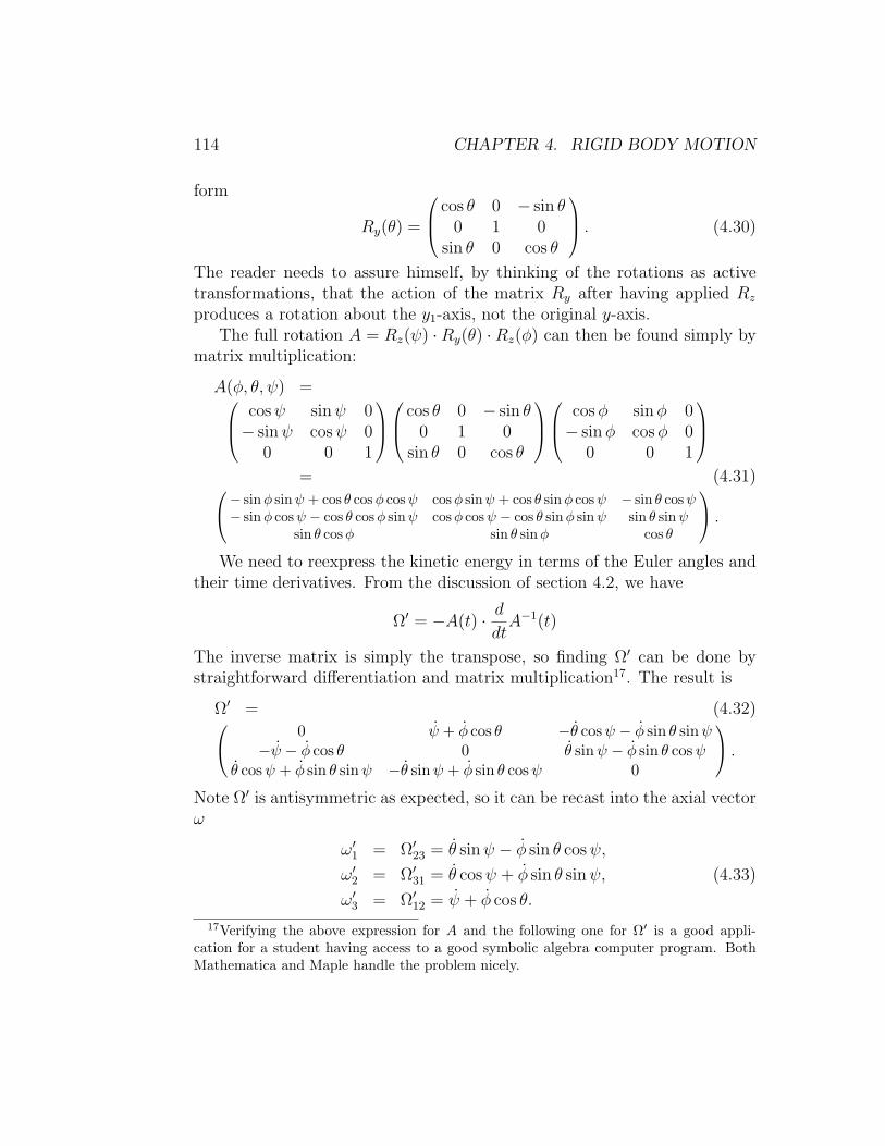
114 CHAPTER 4. RIGID BODY MOTION
form
Ry(θ) =
cos θ 0 − sin θ0 1 0
sin θ 0 cos θ
. (4.30)
The reader needs to assure himself, by thinking of the rotations as activetransformations, that the action of the matrix Ry after having applied Rz
produces a rotation about the y1-axis, not the original y-axis.The full rotation A = Rz(ψ) ·Ry(θ) ·Rz(φ) can then be found simply by
matrix multiplication:
A(φ, θ, ψ) = cosψ sinψ 0− sinψ cosψ 0
0 0 1
cos θ 0 − sin θ
0 1 0sin θ 0 cos θ
cosφ sinφ 0− sinφ cosφ 0
0 0 1
= (4.31)− sinφ sinψ + cos θ cosφ cosψ cosφ sinψ + cos θ sinφ cosψ − sin θ cosψ
− sinφ cosψ − cos θ cosφ sinψ cosφ cosψ − cos θ sinφ sinψ sin θ sinψsin θ cosφ sin θ sinφ cos θ
.We need to reexpress the kinetic energy in terms of the Euler angles and
their time derivatives. From the discussion of section 4.2, we have
Ω′ = −A(t) · ddtA−1(t)
The inverse matrix is simply the transpose, so finding Ω′ can be done bystraightforward differentiation and matrix multiplication17. The result is
Ω′ = (4.32) 0 ψ + φ cos θ −θ cosψ − φ sin θ sinψ−ψ − φ cos θ 0 θ sinψ − φ sin θ cosψ
θ cosψ + φ sin θ sinψ −θ sinψ + φ sin θ cosψ 0
.Note Ω′ is antisymmetric as expected, so it can be recast into the axial vectorω
ω′1 = Ω′23 = θ sinψ − φ sin θ cosψ,
ω′2 = Ω′31 = θ cosψ + φ sin θ sinψ, (4.33)
ω′3 = Ω′12 = ψ + φ cos θ.
17Verifying the above expression for A and the following one for Ω′ is a good appli-cation for a student having access to a good symbolic algebra computer program. BothMathematica and Maple handle the problem nicely.

4.4. DYNAMICS 115
This expression for ~ω gives the necessary velocities for the kinetic energyterm (4.20 or 4.22) in the Lagrangian, which becomes
L =1
2MV 2 +MV ·
(~ω × ~B
)+
1
2~ω · I(R) · ~ω − U(R, θ, ψ, φ), (4.34)
or
L =1
2M~V 2 +
1
2~ω · I(cm) · ~ω − U(~R, θ, ψ, φ), (4.35)
with ~ω =∑i ω′ie′i given by (4.33).
4.4.3 The symmetric top
Now let us consider an example with external forces which constrain onepoint of a symmetrical top to be stationary. Then we choose this to be thefixed point, at the origin R = 0, and we choose the body-fixed z′-axis to bealong the axis of symmetry. Of course the center of mass in on this axis,so ~R = (0, 0, `) in body-fixed coordinates. We will set up the motion bywriting the Lagrangian from the forms for the kinetic and potential energy,due entirely to the gravitational field18.
T =1
2(ω2
1 + ω22)I1 +
1
2ω2
3I3
=1
2
(φ2 sin2 θ + θ2
)I1 +
1
2
(φ cos θ + ψ
)2I3, (4.36)
U = Mgzcm = Mg`(A−1
)zz
= Mg` cos θ. (4.37)
So L = T − U is independent of φ, ψ, and the corresponding momenta
pφ = φ sin2 θI1 +(φ cos θ + ψ
)cos θI3
= φ sin2 θI1 + cos θω3I3,
pψ =(φ cos θ + ψ
)I3 = ω3I3
are constants of the motion. Let us use parameters a = pψ/I1 and b = pφ/I1,which are more convenient, to parameterize the motion, instead of pφ, pψ, or
18As we did in discussing Euler’s equations, we drop the primes on ωi and on Iij eventhough we are evaluating these components in the body fixed coordinate system. Thecoordinate z, however, is still a lab coordinate, with ez pointing upward.

116 CHAPTER 4. RIGID BODY MOTION
even ω3, which is also a constant of the motion and might seem physically amore natural choice. A third constant of the motion is the energy,
E = T + U =1
2I1
(θ2 + φ2 sin2 θ
)+
1
2ω2
3I3 +Mg` cos θ.
Solving for φ from pφ = I1b = φ sin2 θI1 + I1a cos θ,
φ =b− a cos θ
sin2 θ, (4.38)
ψ = ω3 − φ cos θ =I1a
I3
− b− a cos θ
sin2 θcos θ, (4.39)
Then E becomes
E =1
2I1θ
2 + U ′(θ) +1
2I3ω
23,
where
U ′(θ) :=1
2I1
(b− a cos θ)2
sin2 θ+Mg` cos θ.
The term 12I3ω
23 is an ignorable constant, so we consider E ′ := E − 1
2I3ω
23
as the third constant of the motion, and we now have a one dimensionalproblem for θ(t), with a first integral of the motion. Once we solve for θ(t),we can plug back in to find φ and ψ.
Substitute u = cos θ, u = − sin θθ, so
E ′ =I1u
2
2(1− u2)+
1
2I1
(b− au)2
1− u2+Mg`u,
or
u2 = (1− u2)(α− βu)− (b− au)2 =: f(u), (4.40)
with α = 2E ′/I1, β = 2Mg`/I1.f(u) is a cubic with a positive u3
term, and is negative at u = ±1,where the first term vanishes, andwhich are also the limits of thephysical range of values of u. Ifthere are to be any allowed val-ues for u2, f(u) must be nonneg-ative somewhere in u ∈ [−1, 1], sof must look very much like what isshown.
. 2u
θ
θ
mincos
maxcos u1
-1

4.4. DYNAMICS 117
To visualize what is happening, note that a point on the symmetry axis moveson a sphere, with θ and φ representing the usual spherical coordinates, ascan be seen by examining what A−1 does to (0, 0, z′). So as θ moves backand forth between θmin and θmax, the top is wobbling closer and furtherfrom the vertical, called nutation. At the same time, the symmetry axis
θ′ = 52 θ′ = 44 θ′ = θmin
Figure 4.3: Possible loci for a point on the symmetry axis of the top. Theaxis nutates between θmin = 50 and θmax = 60
is precessing, rotating about the vertical axis, at a rate φ which is notconstant but a function of θ (Eq. 4.38). Qualitatively we may distinguishthree kinds of motion, depending on the values of φ at the turning points inθ. These in turn depend on the initial conditions and the parameters of thetop, expressed in a, b, and θmin, θmax. If the value of u′ = cos θ′ at whichφ vanishes is within the range of nutation, then the precession will be indifferent directions at θmin and θmax, and the motion is as in Fig. 4.3a. Onthe other hand, if θ′ = cos−1(b/a) 6∈ [θmin, θmax], the precession will alwaysbe in the same direction, although it will speed up and slow down. We thenget a motion as in Fig. 4.3b. Finally, it is possible that cos θmin = b/a, sothat the precession stops at the top, as in Fig. 4.3c. This special case is ofinterest, because if the top’s axis is held still at an angle to the vertical, andthen released, this is the motion we will get.
Exercises
4.1 Prove the following properties of matrix algebra:(a) Matrix multiplication is associative: A · (B · C) = (A ·B) · C.

118 CHAPTER 4. RIGID BODY MOTION
(b) (A ·B)T = BT ·AT , where AT is the transpose of A, that is (AT )ij := Aji.(c) If A−1 and B−1 exist, (A ·B)−1 = B−1 ·A−1.(d) The complex conjugate of a matrix (A∗)ij = A∗ij is the matrix with everyelement complex conjugated. The hermitean conjugate A† is the transpose ofthat, A† := (A∗)T = (AT )∗, with (A†)ij := A∗ji. Show that (A ·B)∗ = A∗ ·B∗ and(A ·B)† = B† ·A†.
4.2 In section (4.1) we considered reexpressing a vector ~V =∑i Viei in terms of
new orthogonal basis vectors. If the new vectors are ~e ′i =∑j Aij ej , we can also
write ei =∑j Aji~e
′j , because AT = A−1 for an orthogonal transformation.
Consider now using a new basis ~e ′i which are not orthonormal. Then we mustchoose which of the two above expressions to generalize. Let ei =
∑j Aji~e
′j , and
find the expressions for (a) ~e ′j in terms of ei; (b) V ′i in terms of Vj ; and (c) Vi interms of V ′j . Then show (d) that if a linear tranformation T which maps vectors~V → ~W is given in the ei basis by a matrix Bij , in that Wi =
∑BijVj , then
the same transformation T in the ~e ′i basis is given by C = A · B · A−1. Thistransformation of matrices, B → C = A · B · A−1, for an arbitrary invertiblematrix A, is called a similarity transformation.
4.3 Two matrices B and C are called similar if there exists an invertible matrixA such that C = A · B · A−1, and this transformation of B into C is called asimilarity transformation, as in the last problem. Show that, if B and C are similar,(a) TrB = TrC; (b) detB = detC; (c) B and C have the same eigenvalues; (d) IfA is orthogonal and B is symmetric (or antisymmetric), then C is symmetric (orantisymmetric).
4.4 From the fact that AA−1 = 1 for any invertible matrix, show that if A(t) isa differentiable matrix-valued function of time,
A A−1 = −AdA−1
dt.
4.5 Show that a counterclockwise rotation through an angle θ about an axis inthe direction of a unit vector n passing through the origin is given by the matrix
Aij = δij cos θ + ninj(1− cos θ)− εijknk sin θ.

4.4. DYNAMICS 119
4.6 Consider a rigid body in the shape of a right circular cone of height h and abase which is a circle of radius R, made of matter with a uniform density ρ.a) Find the position of the center ofmass. Be sure to specify with respectto what.b) Find the moment of inertia ten-sor in some suitable, well specified co-ordinate system about the center ofmass.c) Initially the cone is spinning aboutits symmetry axis, which is in the zdirection, with angular velocity ω0,and with no external forces or torquesacting on it. At time t = 0 it is hitwith a momentary laser pulse whichimparts an impulse P in the x direc-tion at the apex of the cone, as shown.
R
h
P
y
x
Describe the subsequent force-free motion, including, as a function of time, theangular velocity, angular momentum, and the position of the apex, in any inertialcoordinate system you choose, provided you spell out the relation to the initialinertial coordinate system.
4.7 We defined the general rotation as A = Rz(ψ) · Ry(θ) · Rz(φ). Work outthe full expression for A(φ, θ, ψ), and verify the last expression in (4.31). [Forthis and exercise 4.8, you might want to use a computer algebra program such asmathematica or maple, if one is available.]
4.8 Find the expression for ~ω in terms of φ, θ, ψ, φ, θ, ψ. [This can be done simplywith computer algebra programs. If you want to do this by hand, you might findit easier to use the product form A = R3R2R1, and the rather simpler expressionsfor RRT . You will still need to bring the result (for R1R
T1 , for example) through
the other rotations, which is somewhat messy.]
4.9 A diamond shaped object is shown in top, front, and side views. It is anoctahedron, with 8 triangular flat faces.

120 CHAPTER 4. RIGID BODY MOTION
It is made of solid aluminum of uniformdensity, with a total mass M . The di-mensions, as shown, satisfy h > b > a.(a) Find the moment of inertia tensorabout the center of mass, clearly speci-fying the coordinate system chosen.(b) About which lines can a stable spin-ning motion, with fixed ~ω, take place,assuming no external forces act on thebody? C’
B’
C
A B
h
h
a
a
A B A’
C’
C
b b a a
B’ B
A
A’
C
4.10 From the expression 4.40 for u = cos θ for the motion of the symmetric top,we can derive a function for the time t(u) as an indefinite integral
t(u) =∫ u
f−1/2(z) dz.
For values which are physically realizable, the function f has two (generically dis-tinct) roots, uX ≤ uN in the interval u ∈ [−1, 1], and one root uU ∈ [1,∞), whichdoes not correspond to a physical value of θ. The integrand is then generically ananalytic function of z with square root branch points at uN , uX , uU , and∞, whichwe can represent on a cut Riemann sheet with cuts on the real axis, [−∞, uX ] and[uN , uU ], and f(u) > 0 for u ∈ (uX , uN ). Taking t = 0 at the time the top is atthe bottom of a wobble, θ = θmax, u = uX , we can find the time at which it firstreaches another u ∈ [uX , uN ] by integrating along the real axis. But we could alsouse any other path in the upper half plane, as the integral of a complex functionis independent of deformations of the path through regions where the function isanalytic.(a) Extend this definition to a function t(u) defined for Im u ≥ 0, with u not on acut, and show that the image of this function is a rectangle in the complex t plane,and identify the pre-images of the sides. Call the width T/2 and the height τ/2(b) Extend this function to the lower half of the same Riemann sheet by allowingcontour integrals passing through [uX , uN ], and show that this extends the imagein t to the rectangle (0, T/2)× (−iτ/2, iτ/2).(c) If the coutour passes through the cut (−∞, uX ] onto the second Riemann sheet,the integrand has the opposite sign from what it would have at the correspondingpoint of the first sheet. Show that if the path takes this path onto the second sheet

4.4. DYNAMICS 121
and reaches the point u, the value t1(u) thus obtained is t1(u) = −t0(u), wheret0(u) is the value obtained in (a) or (b) for the same u on the first Riemann sheet.(d) Show that passing to the second Riemann sheet by going through the cut[uN , uU ] instead, produces a t2(u) = t1 + T .(e) Show that evaluating the integral along two contours, Γ1 and Γ2, which differonly by Γ1 circling the [uN , uU ] cut clockwise once more than Γ2 does, gives t1 =t2 + iτ .(f) Show that any value of t can be reached by some path, by circling the [uN , uU ]as many times as necessary, and also by passing downwards through it and upwardsthrough the [−∞, uX ] cut as often as necessary (perhaps reversed).(g) Argue that thus means the function u(t) is an analytic function from thecomplex t plane into the u complex plane, analytic except at the points t = nT +i(m+ 1
2)τ , where u(t) has double poles. Note this function is doubly periodic, withu(t) = u(t+ nT + imτ).(g) Show that the function is then given by u = β ℘(t − iτ/2) + c, where c is aconstant, β is the constant from (4.40), and
℘(z) =1z2
+∑m,n∈ZZ
(m,n)6=0
(1
(z − nT −miτ)2− 1
(nT +miτ)2
)
is the Weierstrass’ ℘-Function.(h) Show that ℘ satisfies the differential equation
℘′2 = 4℘3 − g2℘− g3,
where
g2 =∑
m,n∈Z(m,n)6=(0,0)
(mT + inτ)−4, g3 =∑
m,n∈Z(m,n)6=(0,0)
(mT + inτ)−6.
[Note that the Weierstrass function is defined more generally, using parametersω1 = T/2, ω2 = iτ/2, with the ω’s permitted to be arbitrary complex numberswith differing phases.]
4.11 As a rotation about the origin maps the unit sphere into itself, one wayto describe rotations is as a subset of maps f : S2 → S2 of the (surface of the)unit sphere into itself. Those which correspond to rotations are clearly one-to-one, continuous, and preserve the angle between any two paths which intersectat a point. This is called a conformal map. In addition, rotations preserve thedistances between points. In this problem we show how to describe such mappings,and therefore give a representation for the rotations in three dimensions.

122 CHAPTER 4. RIGID BODY MOTION
(a) Let N be the north pole (0, 0, 1) of the unit sphere Σ = (x, y, z), x2 +y2 +z2 =1. Define the map from the rest of the sphere s : Σ − N → R2 given by astereographic projection, which maps each point on the unit sphere, other thanthe north pole, into the point (u, v) in the equatorial plane (x, y, 0) by giving theintersection with this plane of the straight line which joins the point (x, y, z) ∈ Σto the north pole. Find (u, v) as a function of (x, y, z), and show that the lengthsof infinitesimal paths in the vicinity of a point are scaled by a factor 1/(1 − z)independent of direction, and therefore that the map s preserves the angles betweenintersecting curves (i.e. is conformal).(b) Show that the map f((u, v)) → (u′, v′) which results from first applying s−1,then a rotation, and then s, is a conformal map from R2 into R2, except for thepre-image of the point which gets mapped into the north pole by the rotation.By a general theorem of complex variables, any such map is analytic, so f : u+iv →u′ + iv′ is an analytic function except at the point ξ0 = u0 + iv0 which is mappedto infinity, and ξ0 is a simple pole of f . Show that f(ξ) = (aξ + b)/(ξ − ξ0), forsome complex a and b. This is the set of complex Mobius transformations, whichare usually rewritten as
f(ξ) =αξ + β
γξ + δ,
where α, β, γ, δ are complex constants. An overall complex scale change does notaffect f , so the scale of these four complex constants is generally fixed by imposinga normalizing condition αδ − βγ = 1.(c) Show that composition of Mobius transformations f ′′ = f ′ f : ξ −→
fξ′ −→
f ′ξ′′
is given by matrix multiplication,(α′′ β′′
γ′′ δ′′
)=(α′ β′
γ′ δ′
)·(α βγ δ
).
(d) Not every mapping s−1 f s is a rotation, for rotations need to preservedistances as well. We saw that an infinitesimal distance d` on Σ is mapped by s toa distance |dξ| = d`/(1− z). Argue that the condition that f : ξ → ξ correspondto a rotation is that d˜≡ (1 − z)|df/dξ||dξ| = d`. Express this change of scale interms of ξ and ξ rather than z and z, and find the conditions on α, β, γ, δ thatinsure this is true for all ξ. Together with the normalizing condition, show that thisrequires the matrix for f to be a unitary matrix with determinant 1, so that theset of rotations corresponds to the group SU(2). The matrix elements are calledCayley-Klein parameters, and the real and imaginary parts of them are called theEuler parameters.

Chapter 5
Small Oscillations
5.1 Small oscillations about stable equilibrium
Consider a situation with N unconstrained generalized coordinates qi de-scribed by a mass matrix Mij(qk) and a potential U(qi), and supposethat U has a local minimum at some point in configuration space, qi = qi0.Then this point is a stable equilibrium point, for the generalized force at thatpoint is zero, and if the system is placed nearly at rest near that point, it willnot have enough energy to move far away from that point. We may studythe behavior of such motions by expanding the potential1 in Taylor’s seriesexpansion in the deviations ηi = qi − qi0,
U(q1, . . . , qN) = U(qi0) +∑i
∂U
∂qi
∣∣∣∣∣0
ηi +1
2
∑ij
∂2U
∂qi∂qj
∣∣∣∣∣0
ηiηj + ... .
The constant U(qi0) is of no interest, as only changes in potential matter,so we may as well set it to zero. In the second term, − ∂U/∂qi|0 is thegeneralized force at the equilibrium point, so it is zero. Thus the leadingterm in the expansion is the quadratic one, and we may approximate
U(qi) =1
2
∑ij
Aijηiηj, with Aij =∂2U
∂qi∂qj
∣∣∣∣∣0
. (5.1)
Note that A is a constant symmetric real matrix.
1assumed to have continuous second derivatives.
123

124 CHAPTER 5. SMALL OSCILLATIONS
The kinetic energy T = 12
∑Mij ηiηj is already second order in the small
variations from equilibrium, so we may evaluate Mij, which in general candepend on the coordinates qi, at the equilibrium point, ignoring any higherorder changes. Thus Mij is a constant. Thus both the kinetic and potentialenergies are quadratic forms in the displacement η, which we think of as avector in N -dimensional space. Thus we can write the energies in matrixform
T =1
2ηT ·M · η, U =
1
2ηT · A · η. (5.2)
A and M are real symmetric matrices, and because any displacement corre-sponds to positive kinetic and nonnegative potential energies, they are pos-itive (semi)definite matrices, meaning that all their eigenvalues are greaterthan zero, except that A may also have eigenvalues equal to zero (theseare directions in which the stability is neutral to lowest order, but may bedetermined by higher order terms in the displacement).
Lagrange’s equation of motion
0 =d
dt
∂L
∂ηi− ∂L
∂ηi=
d
dtM · η + A · η = M · η + A · η (5.3)
is not necessarily diagonal in the coordinate η. We shall use the fact thatany real symmetric matrix can be diagonalized by a similarity transforma-tion with an orthogonal matrix to reduce the problem to a set of independantharmonic oscillators. While both M and A can be diagonalized by an orthog-onal transformation, they can not necessarily be diagonalized by the sameone, so our procedure will be in steps:
1. Diagonalize M with an orthogonal transformationO1, transforming thecoordinates to a new set x = O1 · η.
2. Scale the x coordinates to reduce the mass matrix to the identity ma-trix. The new coordinates will be called y.
3. Diagonalize the new potential energy matrix with another orthogonalmatrix O2, giving the final set of coordinates, ξ = O2 · y. Note thistransformation leaves the kinetic energy matrix diagonal because theidentity matrix is unaffected by similarity transformations.
The ξ are normal modes, modes of oscillation which are independent inthe sense that they do not affect each other.

5.1. SMALL OSCILLATIONS ABOUT STABLE EQUILIBRIUM 125
Let us do this in more detail. We are starting with the coordinates η andthe real symmetric matrices A and M , and we want to solve the equationsM · η + A · η = 0. In our first step, we use the matrix O1, which linearalgebra guarantees exists, that makes m = O1 ·M ·O−1
1 diagonal. Note O1 istime-independent, so defining xi =
∑j O1 ijηj also gives xi =
∑j O1 ij ηj, and
T =1
2ηT ·M · η
=1
2ηT ·
(O−1
1 ·m · O1
)· η
=1
2
(ηT · OT1
)·m · (O1 · η)
=1
2(O1 · η)T ·m · (O1 · η)
=1
2xT ·m · x.
Similarly the potential energy becomes U = 12xT · O1 · A · O−1
1 · x. We knowthat the matrix m is diagonal, and the diagonal elements mii are all strictlypositive. To begin the second step, define the diagonal matrix Sij =
√miiδij
and new coordinates yi = Siixi =∑j Sijxj, or y = S·x. Nowm = S2 = ST ·S,
so T = 12xT ·m · x = 1
2xT · ST · S · x = 1
2(S · x)T · S · x = 1
2yT · y. In terms of
y, the potential energy is U = 12yT ·B · y, where
B = S−1 · O1 · A · O−11 · S−1
is still a symmetric matrix2.Finally, let O2 be an orthogonal matrix which diagonalizes B, so C =
O2 ·B · O−12 is diagonal, and let ξ = O2 · y. Just as in the first step,
U =1
2ξT · O2 ·B · O−1
2 · ξ =1
2ξT · C · ξ,
while the kinetic energy
T =1
2yT · y =
1
2yT · OT2 · O2 · y =
1
2ξT · ξ
is still diagonal. Because the potential energy must still be nonnegative, allthe diagonal elements Cii are nonnegative, and we will call them ωi :=
√Cii.
2O1 ·A · O−11 is symmetric because A is and O1 is orthogonal, so O−1
1 = OT1 .

126 CHAPTER 5. SMALL OSCILLATIONS
Then
T =1
2
∑j
ξ2j , U =
1
2
∑j
ω2j ξ
2j , ξj + ω2
j ξj = 0,
so we have N independent harmonic oscillators with the solutions
ξj = Re ajeiωjt,
with some arbitrary complex numbers aj.To find what the solution looks like in terms of the original coordinates
qi, we need to undo all these transformations. As ξ = O2 · y = O2 · S · x =O2 · S · O1 · η, we have
q = q0 +O−11 · S−1 · O−1
2 · ξ.
We have completely solved this very general problem in small oscilla-tions, at least in the sense that we have reduced it to a solvable problem ofdiagonalizing symmetric real matrices. What we have done may appear ab-stract and formal and devoid of physical insight, but it is a general algorithmwhich will work on a very wide class of problems of small oscillations aboutequilibrium. In fact, because diagonalizing matrices is something for whichcomputer programs are available, this is even a practical method for solvingsuch systems, even if there are dozens of interacting particles.
5.1.1 Molecular Vibrations
Consider a molecule made up of n atoms. We need to choose the right levelof description to understand low energy excitations. We do not want todescribe the molecule in terms of quarks, gluons, and leptons. Nor do weneed to consider all the electronic motion, which is governed by quantummechanics. The description we will use, called the Born-Oppenheimerapproximation, is to model the nuclei as classical particles. The electrons,which are much lighter, move around much more quickly and cannot betreated classically; we assume that for any given configuration of the nuclei,the electrons will almost instantaneously find a quantum-mechanical groundstate, which will have an energy which depends on the current positions ofthe nuclei. This is then a potential energy when considering the nuclearmotion. The nuclei themselves will be considered point particles, and we

5.1. SMALL OSCILLATIONS ABOUT STABLE EQUILIBRIUM 127
will ignore internal quantum-mechanical degrees of freedom such as nuclearspins. So we are considering n point particles moving in three dimensions,with some potential about which we know only qualitative features. Thereare 3n degrees of freedom. Of these, 3 are the center of mass motion, which,as there are no external forces, is simply motion at constant velocity. Someof the degrees of freedom describe rotational modes, i.e. motions that themolecule could have as a rigid body. For a generic molecule this would bethree degrees of freedom, but if the equilibrium configuration of the moleculeis linear, rotation about that line is not a degree of freedom, and so only twoof the degrees of freedom are rotations in that case. The remaining degreesof freedom, 3n − 6 for noncollinear and 3n − 5 for collinear molecules, arevibrations.
O2 CO2 H O2
Figure 5.1: Some simple molecules in their equilibrium positions.
For a collinear molecule, it makes sense to divide the vibrations intotransverse and longitudinal ones. Considering motion in one dimension only,the nuclei have n degrees of freedom, one of which is a center-of-mass motion,leaving n− 1 longitudinal vibrations. So the remaining (3n− 5)− (n− 1) =2(n − 2) vibrational degrees of freedom are transverse vibrational modes.There are no such modes for a diatomic molecule.
Example: CO2
Consider first the CO2 molecule. As it is a molecule, there must be a positionof stable equilibrium, and empirically we know it to be collinear and sym-metric, which one might have guessed. We will first consider only collinearmotions of the molecule. If the oxygens have coordinates q1 and q2, and thecarbon q3, the potential depends on q1 − q3 and q2 − q3 in the same way, so

128 CHAPTER 5. SMALL OSCILLATIONS
the equilibrium positions have q2 − q3 = −(q1 − q3) = b. Assuming no directforce between the two oxygen molecules, the one dimensional motion may bedescribed near equilibrium by
U =1
2k(q3 − q1 − b)2 +
1
2k(q2 − q3 − b)2
T =1
2mOq
21 +
1
2mOq
22 +
1
2mC q
23.
We gave our formal solution in terms of displacements from the equilibriumposition, but we now have a situation in which there is no single equilibriumposition, as the problem is translationally invariant, and while equilibriumhas constraints on the differences of q’s, there is no constraint on the centerof mass. We can treat this in two different ways:
1. Explicitly fix the center of mass, eliminating one of the degrees of free-dom.
2. Pick arbitrarily an equilibrium position. While the deviations of thecenter-of-mass position from the equilibrium is not confined to smallexcursions, the quadratic approximation is still exact.
First we follow the first method. We can always work in a frame wherethe center of mass is at rest, at the origin. Then mO(q1 + q2) + mCq3 = 0is a constraint, which we must eliminate. We can do so by dropping q3
as an independant degree of freedom, and we have, in terms of the twodisplacements from equilibrium η1 = q1 + b and η2 = q2 − b, q3 = −(η1 +η2)mO/mC , and
T =1
2mO(η2
1 + η22) +
1
2mC η
23 =
1
2mO
[η2
1 + η22 +
mO
mC
(η1 + η2)2]
=1
2
m2O
mC
( η1 η2 )(
1 +mC/mO 11 1 +mC/mO
)(η1
η2
).
Now T is not diagonal, or more precisely M isn’t. We must find the orthog-onal matrix O1 such that O1 ·M · O−1
1 is diagonal. We may assume it to bea rotation, which can only be
O =(
cos θ − sin θsin θ cos θ
)

5.1. SMALL OSCILLATIONS ABOUT STABLE EQUILIBRIUM 129
for some value of θ. It is worthwhile to derive a formula for diagonalizing ageneral real symmetric 2 × 2 matrix and then plug in our particular form.Let
M =(a bb d
), and O =
(c −ss c
),
where we have abbreviated s = sin θ, c = cos θ. We will require the matrixelement m12 = (O ·M · O−1)12 = 0, because m is diagonal. This determinesθ:
O ·M · O−1 =(c −ss c
)(a bb d
)(c s−s c
)=
(c −s· ·
)( · as+ bc· bs+ cd
)=( · acs+ bc2 − bs2 − scd· ·
)where we have placed a · in place of matrix elements we don’t need to cal-culate. Thus the condition on θ is
(a− d) sin θ cos θ + b(cos2 θ − sin2 θ) = 0 =1
2(a− d) sin 2θ + b cos 2θ,
or
tan 2θ =−2b
a− d.
Notice this determines 2θ only modulo π, and therefore θ modulo 90, whichought to be expected, as a rotation through 90 only interchanges axes andreverses directions, both of which leave a diagonal matrix diagonal.
In our case a = d, so tan 2θ =∞, and θ = π/4. As x = O1η,(x1
x2
)=(
cosπ/4 − sin π/4sin π/4 cos π/4
)(η1
η2
)=
1√2
(η1 − η2
η1 + η2
),
and inversely (η1
η2
)=
1√2
(x1 + x2
−x1 + x2
).
Then
T =1
2mO
[(x1 + x2)2
2+
(x1 − x2)2
2+mO
mC
(√
2x2)2
]

130 CHAPTER 5. SMALL OSCILLATIONS
=1
2mOx
21 +
1
2mO
(1 +
2mO
mC
)x2
2
U =1
2k(q3 − q1 − b)2 +
1
2k(q2 − q3 − b)2
=1
2k
[(η1 +
mO
mC
(η1 + η2))2
+(η2 +
mO
mC
(η1 + η2))2]
=1
2k
[η2
1 + η22 +
2m2O
m2C
(η1 + η2)2 +2mO
mC
(η1 + η2)2
]
=1
2k
[x2
1 + x22 +
4mO
m2C
(mO +mC)x22
]
=1
2kx2
1 +1
2k(mC + 2mO
mC
)2
x22.
Thus U is already diagonal and we don’t need to go through steps 2 and 3,the scaling and second orthogonalization, except to note that if we skip thescaling the angular frequencies are given by ω2
i = coefficient in U / coefficient
in T . Thus we have one normal mode, x1, with ω1 =√k/mO, with x2 = 0,
η1 = −η2, q3 = 0, in which the two oxygens vibrate in and out together,symmetrically about the carbon, which doesn’t move. We also have anothermode, x2, with
ω2 =
√√√√k(mC + 2mO)2/m2O
mO(1 + 2mO/mC)=
√k(mC + 2mO)
mOmC
,
with x1 = 0, η1 = η2, in which the two oxygens move right or left together,with the carbon moving in the opposite direction.
We have successfully solved for the longitudinal vibrations by eliminatingone of the degrees of freedom. Let us now try the second method, in whichwe choose an arbitrary equilibrium position q1 = −b, q2 = b, q3 = 0. Then
T =1
2mO(η2
1 + η22) +
1
2mC η
23
U =1
2k[(η1 − η3)2 + (η2 − η3)2
].
T is already diagonal, so O1 = 1I, x = η. In the second step S is the diagonalmatrix with S11 = S22 =
√mO, S33 =
√mC , and yi =
√mOηi for i = 1, 2,

5.1. SMALL OSCILLATIONS ABOUT STABLE EQUILIBRIUM 131
and y3 =√mCη3. Then
U =1
2k
( y1√mO
− y3√mC
)2
+
(y2√mO
− y3√mC
)2
=1
2
k
mOmC
[mCy
21 +mCy
22 + 2mOy
23 − 2
√mOmC(y1 + y2)y3
].
Thus the matrix B is
B =
mC 0 −√mOmC
0 mC −√mOmC
−√mOmC −√mOmC 2mO
,which is singular, as it annihilates the vector yT = (
√mO,√mO,√mC),
which corresponds to ηT = (1, 1, 1), i.e. all the nuclei are moving by the sameamount, or the molecule is translating rigidly. Thus this vector correspondsto a zero eigenvalue of U , and a harmonic oscillation of zero frequency. This isfree motion3, ξ = ξ0+vt. The other two modes can be found by diagonalizingthe matrix, and will be as we found by the other method.
Transverse motion
What about the transverse motion? Consider the equilibrium position ofthe molecule to lie in the x direction, and consider small deviations in the zdirection. The kinetic energy
T =1
2mOz1 +
1
2mOz
22 +
1
2mC z
23 .
is already diagonal, just as forthe longitudinal modes in the sec-ond method. Any potential en-ergy must be due to a resistanceto bending, so to second order,U ∝ (ψ − θ)2 ∼ (tanψ − tan θ)2 =[(z2−z3)/b+(z1−z3)/b]2 = b−2(z1+z2 − 2z3)2.
ψθ 2
31
z
zbz
b
Note that the potential energy is proportional to the square of a single linear
3To see that linear motion is a limiting case of harmonic motion as ω → 0, we need tochoose the complex coefficient to be a function of ω, A(ω) = x0 − iv0/ω, with x0 and v0real. Then x(t) = limω→0 Re A(ω)eiωt = x0 + v0 limω→0 sin(ωt)/ω = x0 + v0t

132 CHAPTER 5. SMALL OSCILLATIONS
combination of the displacements, or to the square of one component (withrespect to a particular direction) of the displacement. Therefore there is nocontribution of the two orthogonal directions, and there are two zero modes,or two degrees of freedom with no restoring force. One of these is the center ofmass motion, z1 = z2 = z3, and the other is the third direction in the abstractspace of possible displacements, zT = (1,−1, 0), with z1 = −z2, z3 = 0, whichwe see is a rotation. Thus there remains only one true transverse vibrationalmode in the z direction, and also one in the y direction, which together withthe two longitudinal ones we found earlier, make up the 4 vibrational modeswe expected from the general formula 2(n− 2) for a collinear molecule.
You might ask whether these oscillations we have discussed are in anyway observable. Quantum mechanically, a harmonic oscillator can only be instates with excitation energy E = nhω, where n ∈ Z is an integer and 2πhis Planck’s constant. When molecules are in an excited state, they can emita photon while changing to a lower energy state. The energy of the photon,which is the amount lost by the molecule, is proportional to the frequency,∆E = 2πhf , so by measuring the wavelength of the emitted light, we candetermine the vibrational frequencies of the molecules. So the calculationswe have done, and many others for which we have built the apparatus, arein fact very practical tools for molecular physics.
5.1.2 An Alternative Approach
The step by step diagonalization we just gave is not the easiest approach tosolving the linear differential equation (5.3). Solutions to linear differentialequations are subject to superposition, and equations with coefficients inde-pendent of time are simplified by Fourier transform, so we can express theN dimensional vector of functions ηj(t) as
ηj(t) =∫ ∞−∞
dωψj(ω)e−iωt.
Then the Lagrange equations become∫ ∞−∞
dω∑j
(Aij − ω2Mij
)ψj(ω)e−iωt = 0 for all t.
But e−iωt are linearly independent functions of t ∈ R, so∑j
(Aij − ω2Mij
)ψj(ω) = 0.

5.2. OTHER INTERACTIONS 133
This implies ψj(ω) = 0 except when the matrix Aij − ω2Mij is singular,det (Aij − ω2Mij) = 0, which gives a discrete set of angular frequenciesω1 . . . ωN , and for each ωj an eigenvector ψj.
5.2 Other interactions
In our treatment we assumed a Lagrangian formulation with a kinetic termpurely quadratic in ~q, together with a velocity independent potential. Thereis a wider scope of small oscillation problems which might include dissipativeforces like friction, or external time-dependent forces, or perhaps terms inthe Lagrangian linear in the velocities. An example of the latter occursin rotating reference frames, from the Coriolus force, and is important inthe question of whether there is a gravitationally stable location for smallobjects caught between the Earth and the moon at the “L5” point4. Each ofthese complications introduces terms, even in the linear approximation to theequations of motion, which cannot be diagonalized away, because there is notsignificant freedom of diagonalization left, in general, after having simplifiedT and U . Thus the approach of section 5.1 does not generalize well, but theapproach of section 5.1.2 can be applied.
For example, we might consider adding a generalized force Qi on ηi, con-sisting of a dissipative force
∑j Rij ηj and a driving force Fi. We will assume
R is a symmetric matrix, as might be a result of a Rayleigh dissipation func-tion (see Section 2.7 or Ref. [6]). We will consider the motion to first orderin F , so any coordinate dependence of R or F is replaced, as it was for Mand A, by their values at the equilibrium position. Thus the equations ofmotion become ∑
j
(Mij ηj +Rij ηj + Aijηj)− Fi = 0.
Again making the ansatz that
ηj(t) =∫ ∞−∞
dωψj(ω)e−iωt
and expressing Fi(t) in terms of its fourier transform
Fj(t) =∫ ∞−∞
dωfi(ω)e−iωt
4See problem 5.3.

134 CHAPTER 5. SMALL OSCILLATIONS
we find ∑j
(−ω2Mij − iωRij + Aij
)ψj = fi.
Except for at most 2N values of ω the matrix multiplying ψj will have a non-zero determinant and will be invertible, allowing us to find the response ψjto the fourier component of the driving force, fi. Those values of ω for whichthe determinant vanishes, and the vector ψj which the matrix annihilates,correspond to damped modes that we would see if the driving force wereremoved.
5.3 String dynamics
In this section we consider two closely related problems, transverse oscilla-tions of a stretched loaded string, and of a stretched heavy string. The latteris is a limiting case of the former. This will provide an introduction to fieldtheory, in which the dynamical degrees of freedom are not a discrete set butare defined at each point in space. In Chapter 8 we will discuss more in-teresting and involved cases such as the electromagnetic field, where at eachpoint in space we have ~E and ~B as degrees of freedom, though not withoutconstraints.
The loaded string we will consider is a light string under tension τ stretchedbetween two fixed points a distance ` apart, say at x = 0 and x = `. Onthe string, at points x = a, 2a, 3a, . . . , na, are fixed n particles each of massm, with the first and last a distance a away from the fixed ends. Thus` = (n+ 1)a. We will consider only small transverse motion of these masses,using yi as the transverse displacement of the i’th mass, which is at x = ia.We assume all excursions from the equilibrium positions yi = 0 are small, andin particular that the difference in successive displacements yi+1 − yi a.Thus we are assuming that the angle made by each segment of the string,θi = tan−1[(yi+1 − yi)/a] 1. Working to first order in the θ’s in the equa-tions of motion, and second order for the Lagrangian, we see that restrictingour attention to transverse motions and requiring no horizontal motion forcestaking the tension τ to be constant along the string. The transverse force onthe i’th mass is thus
Fi = τyi+1 − yi
a+ τ
yi−1 − yia
=τ
a(yi+1 − 2yi + yi−1).

5.3. STRING DYNAMICS 135
The potential energy U(y1, . . . , yn) then satisfies
∂U
∂yi= −τ
a(yi+1 − 2yi + yi−1)
so
U(y1, . . . , yi, . . . , yn)
=∫ yi
0dyi
τ
a(2yi − yi+1 − yi−1) + F (y1, . . . , yi−1, yi+1, . . . , yn)
=τ
a
(y2i − (yi+1 + yi−1)yi
)+ F (y1, . . . , yi−1, yi+1, . . . , yn)
=τ
2a
((yi+1 − yi)2 + (yi − yi−1)2
)+ F ′(y1, . . . , yi−1, yi+1, . . . , yn)
=n∑i=0
τ
2a(yi+1 − yi)2 + constant.
The F and F ′ are unspecified functions of all the yj’s except yi. In the lastexpression we satisfied the condition for all i, and we have used the convenientdefinition y0 = yn+1 = 0. We can and will drop the arbitrary constant.
The kinetic energy is T = 12m∑n
1 y2i .
Before we continue with the analysis of this problem, let us note thatanother physical setup also leads to the same Lagrangian. Consider a onedimensional lattice of identical atoms with a stable equilibrium in which theyare evenly spaced, with interactions between nearest neighbors. Let ηi be thelongitudinal displacement of the i’th atom from its equilibrium position. Thekinetic energy is simply T = 1
2m∑n
1 η2i . As the interatomic distance differs
from its equilibrium position by ηi+1 − ηi, the interaction potential of atomsi and i + 1 can be approximated by U(ηi+1, ηi) ≈ 1
2k(ηi+1 − ηi)2. We have
in effect atoms separated by springs of spring constant k, and we see thatif k = τ/a, we get the same Lagrangian for longitudinal oscillations of thislattice as we had for the transverse oscillations of the loaded string.
As the kinetic energy is simply T = 12m∑n
1 y2i , the mass matrix is already
proportional to the identity matrix and we do not need to go through thefirst two steps of our general process. The potential energy U = 1
2yT · A · y

136 CHAPTER 5. SMALL OSCILLATIONS
has a non-diagonal n× n matrix
A = −τa
−2 1 0 0 · · · 0 01 −2 1 0 · · · 0 00 1 −2 1 · · · 0 0...
......
.... . .
......
0 0 0 0 · · · −2 10 0 0 0 · · · 1 −2
.
Diagonalizing even a 3 × 3 matrix is work, so an n × n matrix might seemout of the question, without some hints from the physics of the situation. Inthis case the hint comes in a roundabout fashion — we will first consider alimit in which n→∞, the continuum limit, which leads to an interestingphysical situation in its own right.
Suppose we consider the loaded string problem in the limit that the spac-ing a becomes very small, but the number of masses m becomes large, keepingthe total length ` of the string fixed. If at the same time we adjust the in-dividual masses so that the mass per unit length, ρ, is fixed, our bumpystring gets smoothed out in the limit, and we might expect that in this limitwe reproduce the physical problem of transverse modes of a uniformly densestretched string, like a violin string. Thus we wish to consider the limit
a→ 0, n→∞, ` = (n+ 1)a fixed, m→ 0, ρ = m/a fixed.
It is natural to think of the degrees of freedom as associated with the label xrather than i, so we redefine the dynamical functions yj(t) as y(x, t), withy(ja, t) = yj(t). While this only defines the function at discrete points in x,these are closely spaced for small a and become dense as a → 0. We willassume that the function y(x) is twice differentiable in the continuum limit,though we shall see that this is not the case for all possible motions of thediscrete system.
What happens to the kinetic and potential energies in this limit? For thekinetic energy,
T =1
2m∑i
y2i =
1
2ρ∑i
ay2(xi) =1
2ρ∑i
∆xy2(xi)→1
2ρ∫ `
0dx y2(x),
where the next to last expression is just the definition of a Riemann integral.For the potential energy,
U =τ
2a
∑i
(yi+1 − yi)2 =τ
2
∑i
∆x(yi+1 − yi
∆x
)2
→ τ
2
∫ `
0dx
(∂y
∂x
)2
.

5.3. STRING DYNAMICS 137
The equation of motion for yi is
myi =∂L
∂yi= −∂U
∂yi=τ
a[(yi+1 − yi)− (yi − yi−1)],
or
ρay(x) =τ
a([y(x+ a)− y(x)]− [y(x)− y(x− a)]).
We need to be careful about taking the limit
y(x+ a)− y(x)
a→ ∂y
∂x
because we are subtracting two such expressions evaluated at nearby points,and because we will need to divide by a again to get an equation betweenfinite quantities. Thus we note that
y(x+ a)− y(x)
a=∂y
∂x
∣∣∣∣∣x+a/2
+O(a2),
so
ρy(x) =τ
a
(y(x+ a)− y(x)
a−y(x)− y(x− a)
a
)
≈ τ
a
∂y∂x
∣∣∣∣∣x+a/2
− ∂y
∂x
∣∣∣∣∣x−a/2
→ τ∂2y
∂x2,
and we wind up with the wave equation for transverse waves on a massivestring
∂2y
∂t2− c2 ∂
2y
∂x2= 0,
where
c =
√τ
ρ.
Solving this wave equation is very simple. For the fixed boundary condi-tions y(x) = 0 at x = 0 and x = `, the solution is a fourier expansion
y(x, t) =∞∑p=1
Re Bpeickpt sin kpx,

138 CHAPTER 5. SMALL OSCILLATIONS
where kp` = pπ. Each p represents one normal mode, and there are aninfinite number as we would expect because in the continuum limit there arean infinite number of degrees of freedom.
We have certainly not shown that y(x) = B sin kx is a normal mode forthe problem with finite n, but it is worth checking it out. This correspondsto a mode with yj = B sin kaj, on which we apply the matrix A
(A · y)i =∑j
Aijyj = −τa
(yi+1 − 2yi + yi−1)
= −τaB (sin(kai+ ka)− 2 sin(kai) + sin(kai− ka))
= −τaB(sin(kai) cos(ka) + cos(kai) sin(ka)− 2 sin(kai)
+ sin(kai) cos(ka)− cos(kai) sin(ka))
=τ
aB (2− 2 cos(ka)) sin(kai)
=2τ
a(1− cos(ka)) yi.
So we see that it is a normal mode, although the frequency of oscillation
ω =
√2τ
am(1− cos(ka)) = 2
√τ
ρ
sin(ka/2)
a
differs from k√τ/ρ except in the limit a→ 0 for fixed k.
The wave numbers k which index the normal modes are restricted bythe fixed ends to the discrete set k = pπ/` = pπ/(n+ 1)a, for p ∈ Z, i.e. p isan integer. This is still too many (∞) for a system with a finite number ofdegrees of freedom. The resolution of this paradox is that not all different k’scorrespond to different modes. For example, if p′ = p + 2m(n + 1) for someinteger m, then k′ = k+ 2πm/a, and sin(k′aj) = sin(kaj+ 2mπ) = sin(kaj),so k and k′ represent the same normal mode. Also, if p′ = 2(n + 1) − p,k′ = (2π/a)−k, sin(k′aj) = sin(2π−kaj) = − sin(kaj), so k and k′ representthe same normal mode, with opposite phase. Finally p = n + 1, k = π/agives yj = B sin(kaj) = 0 for all j and is not a normal mode. This leaves asindependent only p = 1, ..., n, the right number of normal modes for a systemwith n degrees of freedom.
The angular frequency of the p’th normal mode
ωp = 2
√τ
masin
pπ
2(n+ 1)

5.4. FIELD THEORY 139
in plotted in Fig. 5.3. For fixed values of p and ρ, as n→∞,
ωp = 2
√τ
ρ
1
asin
paπ
2`→ 2
√τ
ρ
pπ
2`= ckp,
as we have in the continuum limit.But if we consider modes with afixed ratio of p/n as n → ∞, wedo not have a smooth limit y(x),and such nodes are not appropri-ate for the continuum limit. In thephysics of crystals, the former kindof modes are known as accous-tic modes, while the later modes,in particular those for n − p fixed,which depend on the discrete na-ture of the crystal, are called opti-cal modes.
1 2 3 4 5 6 7 8 9 10 11 12
Fig. 5.3. Frequencies of oscillationof the loaded string.
5.4 Field theory
We now examine how to formulate the continuum limit directly.
5.4.1 Lagrangian density
We saw in the last section that the kinetic and potential energies in thecontinuum limit can be written as integrals over x of densities, and so wemay also write the Lagrangian as the integral of a Lagrangian densityL(x),
L = T − U =∫ L
0dxL(x), L(x) =
1
2ρy2(x, t)− 1
2τ
(∂y(x, t)
∂x
)2 .
This Lagrangian, however, will not be of much use until we figure out what ismeant by varying it with respect to each dynamical degree of freedom or itscorresponding velocity. In the discrete case we have the canonical momentaPi = ∂L/∂yi, where the derivative requires holding all yj fixed, for j 6= i, aswell as all yk fixed. This extracts one term from the sum 1
2ρ∑ay 2
i , and this

140 CHAPTER 5. SMALL OSCILLATIONS
would appear to vanish in the limit a→ 0. Instead, we define the canonicalmomentum as a density, Pi → aP (x = ia), so
P (x = ia) = lim1
a
∂
∂yi
∑i
a L(y(x), y(x), x)|x=ai .
We may think of the last part of this limit,
lima→0
∑i
a L(y(x), y(x), x)|x=ai =∫dxL(y(x), y(x), x),
if we also define a limiting operation
lima→0
1
a
∂
∂yi→ δ
δy(x),
and similarly for 1a∂∂yi
, which act on functionals of y(x) and y(x) by
δy(x1)
δy(x2)= δ(x1 − x2),
δy(x1)
δy(x2)=δy(x1)
δy(x2)= 0,
δy(x1)
δy(x2)= δ(x1 − x2).
Here δ(x′ − x) is the Dirac delta function, defined by its integral,∫ x2
x1
f(x′)δ(x′ − x)dx′ = f(x)
for any function f(x), provided x ∈ (x1, x2). Thus
P (x) =δ
δy(x)
∫ `
0dx′
1
2ρy2(x′, t) =
∫ `
0dx′ρy(x′, t)δ(x′ − x) = ρy(x, t).
We also need to evaluate
δ
δy(x)L =
δ
δy(x)
∫ `
0dx′−τ2
(∂y
∂x
)2
x=x′.
For this we need
δ
δy(x)
∂y(x′)
∂x′=
∂
∂x′δ(x′ − x) := δ′(x′ − x),

5.4. FIELD THEORY 141
which is again defined by its integral,∫ x2
x1
f(x′)δ′(x′ − x)dx′ =∫ x2
x1
f(x′)∂
∂x′δ(x′ − x)dx′
= f(x′)δ(x′ − x)|x2
x1−∫ x2
x1
dx′∂f
∂x′δ(x′ − x)
=∂f
∂x(x),
where after integration by parts the surface term is dropped because δ(x −x′) = 0 for x 6= x′, which it is for x′ = x1, x2 if x ∈ (x1, x2). Thus
δ
δy(x)L = −
∫ `
0dx′τ
∂y
∂x(x′)δ′(x′ − x) = τ
∂2y
∂x2,
and Lagrange’s equations give the wave equation
ρy(x, t)− τ ∂2y
∂x2= 0. (5.4)
We have derived the wave equation for small transverse deformationsof a strectch string by considering the continuum limit of a loaded string,in the process demonstating how to formulate Lagrangian mechanics for acontinuum system. Of course it is more usual, and simpler, to derive itdirectly by considering Newton’s law on an infinitesimal element of the string.Let’s include gravity for good measure. If the string point initially at x
has a transverse displacement y(x)and a longitudinal displacementη(x), both considered small, theslope of the string dy/dx is alsosmall. The segment [x, x+∆x] hasa mass ρ∆x, where as before ρ isthe mass per unit length, and theforces on it are
x x( )∆+( )x x x( )∆+
( )x
τθ θ
∆ xx + x∆
τx
in x direction: τ(x+ ∆x) cos θ(x+ ∆x)− τ(x) cos θ(x) = ρ∆xη
in y direction: τ(x+ ∆x) sin θ(x+ ∆x)− τ(x) sin θ(x)− ρg∆x = ρ∆xy
As θ << 1, we can replace cos θ by 1 and sin θ with tan θ = ∂y/∂x, andthen from the first equation we see that ∂τ/∂x is already small, so we can

142 CHAPTER 5. SMALL OSCILLATIONS
consider τ as constant in the second equation, which gives
τ
(∂y
∂x
∣∣∣∣∣x+∆x
− ∂y
∂x
∣∣∣∣∣x
)− ρg∆x = ρ∆xy,
or
τ∂2y
∂x2− ρg = ρy.
This agrees with Eq. 5.4 if we drop the gravity term, which we had notincluded in our discussion of the loaded string.
5.4.2 Three dimensional continua
Could we do the same kind of analysis on a three dimensional solid object?We might label each piece of the object with an equilibrium or referenceposition ~x, and consider the dynamics of possible displacements ~η(~x). Wewill assume this displacement is small and smooth function of ~x and t, infact twice differentiable. Consider the dynamics of an infinitesimal volumeelement ∆V . The acceleration of each volume element will be determined bythe ratio of the net force on that volume to its mass, ρ∆V , where ρ is now thedensity, mass per unit volume, and is also assumed to be a smooth function,though not necessarily constant. The forces we will consider will be of twotypes. There may be external forces which will be taken to be extensive,that is, proportional to the volume, called volume forces. One example isgravity near the Earth’s surface, with ~F = −ρg∆V ez. If the material underdiscussion had an electric charge density ρE(~x) in an external electric field~E(~x), there would also be a volume force ρE(~x) ~E(~x) ∆V . In addition to thevolume forces, there are also surface forces which the rest of the objectexerts on the element under consideration. We will assume that all suchforces are local, due to the material on the other side of the surface, andcontinuously varying, so the force across an infinitesimal element of surfacedS will be proportional to its area, at least if we keep the direction fixed.
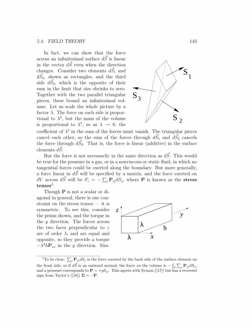
5.4. FIELD THEORY 143
In fact, we can show that the forceacross an infinitesimal surface d~S is linearin the vector d~S even when the directionchanges. Consider two elements d~S1 andd~S2, shown as rectangles, and the thirdside d~S3, which is the opposite of theirsum in the limit that size shrinks to zero.Together with the two parallel triangularpieces, these bound an infinitesimal vol-ume. Let us scale the whole picture by afactor λ. The force on each side is propor-tional to λ2, but the mass of the volumeis proportional to λ3, so as λ → 0, the
S1
S
S 2
3
coefficient of λ2 in the sum of the forces must vanish. The triangular piecescancel each other, so the sum of the forces through d~S1 and d~S2 cancelsthe force through d~S3. That is, the force is linear (additive) in the surface
elements d~S.But the force is not necessarily in the same direction as d~S. This would
be true for the pressure in a gas, or in a nonviscous or static fluid, in which notangential forces could be exerted along the boundary. But more generally,a force linear in d~S will be specified by a matrix, and the force exerted ondV across d~S will be Fi = −∑j PijdSj, where P is known as the stresstensor5.
Though P is not a scalar or di-agonal in general, there is one con-straint on the stress tensor — it issymmetric. To see this, considerthe prism shown, and the torque inthe y direction. The forces acrossthe two faces perpendicular to zare of order λ, and are equal andopposite, so they provide a torque−λ2hPxz in the y direction. Sim-
λ
λh
x
zy
5To be clear:∑j PijdSj is the force exerted by the back side of the surface element on
the front side, so if d~S is an outward normal, the force on the volume is −∫S
∑j PijdSj ,
and a pressure corresponds to P = +pδij . This agrees with Symon ([17]) but has a reversedsign from Taylor’s ([18]) Σ = −P.

144 CHAPTER 5. SMALL OSCILLATIONS
ilarly the two faces perpendicular to x provide a torque +λ2hPzx in thatdirection. The equal forces on other two faces have a moment arm parallelto y and therefore provide no torque in that direction. But the moment ofinertia about the y axis is of order λ2dV = λ4h. So if the angular accelerationis to remain finite as λ→ 0, we must have Pzx −Pxz = 0, and P must be asymmetric matrix.
We expect that the stress forces the material on one side of a boundaryexerts on the other is due to some distortion of the material. Near any valueof x, we may expand the displacement as
ηi(x+ ∆x) = ηi(x) +∂ηi∂xj
∆xj + ...
Moving the entire object as a whole, ~η(x) = constant, or rotating it as a rigidbody about an axis ~ω, with ∂ηi/∂xj = εijkωk, will not produce any stress, andso we will not consider such displacements to be part of the strain tensor,which we therefore define to be the symmetric part of the derivative matrix:
Sij =1
2
(∂ηi∂xj
+∂ηj∂xi
).
In general, the properties of the material will determine how the stress tensoris related to the strain tensor, though for small displacements we expect itto depend linearly.
Even linear dependence could be quite complex, but if the material prop-erties are rotationally symmetric, things are fairly simple. Of course in a crys-tal we might not satisfy that condition, but if we do assume the functionaldependence of the stress on the strain is rotationally invariant, we may findthe most general possibilities by decomposing the tensors into pieces whichbehave suitably under rotations. Here we are generalizing the idea that avector cannot be defined in terms of pure scalars, and a scalar can depend onvectors only through a scalar product. A symmetric tensor consists of a piece,its trace, which behaves like a scalar, and a traceless piece, called the de-viatoric part, which behaves differently, as an irreducible representation6.
6Representations of a symmetry group are defined as vector spaces which are invariantunder the action of the symmetry, and irreducible ones are those for which no propersubspace is closed in that fashion. For more on this, see any book on group theory forphysicists. But for representations of the rotation group a course in quantum mechanicsmay be better. The traceless part of the symmetric tensor transforms like a state withangular momentum 2.

5.4. FIELD THEORY 145
The only possible linear relationships are thus
Tr P = −αTr S; Pij −1
3δij Tr P = −β
(Sij −
1
3δij Tr S
). (5.5)
These are known as the generalized Hooke’s law for an elastic solid.The tensor stress and strain we have described here are perhaps not as fa-
miliar as some other relations met in more elementary courses. First considerthe bulk modulus B, the inverse of the ratio of the fractional decrease involume to the isotropic pressure which causes it. Here the stress and straintensors are both multiples of the identity, P = +pδij and d~η = −cd~x, soS = −cδij and c = p/α. For a linear contraction x→ x− cx the volume willcontract by ∆V = −3cV . Therefore the
bulk modulus B =p
−dV/V=
p
3c=α
3.
Next, consider a shear, in which the displacement might be ~η = cyexproduced by forces ±Fx on thehorizontal faces shown, and ±Fyon the vertical faces. To haveno rotation we need wFx = LFy.The shear modulus G is defined by−Pxy = Fx/A = Gdηx/dy = Gc,where A is the area of the top face.
F
F
FF
x
x
yyw
L
As
Sxy =1
2
(∂ηx∂y
+∂ηy∂x
)=
1
2(c+ 0) =
c
2
and all other components are zero, we can set
β = −Pxy
Sxy= 2G.
Finally, consider a rod being pulled by a force F stretching a distance ∆Lover a length L. Hooke’s constant is k = F/∆L and Young’s modulusY is defined by
F
A= Y
∆L
Lso Y = kL/A.
The strain S11 = ∆L/L, and the stress has −P11 = Y S11, with all othercomponents of the stress zero. But there may be displacement in the trans-verse directions. If the rod is axially symmetric we may assume S22 = S33,

146 CHAPTER 5. SMALL OSCILLATIONS
so
−Tr P = −P11 = Y S11 = αTr S = α (S11 + 2S22) ,
−(P22 −
1
3Tr P
)= 0− Y
3S11 = β
(S22 −
1
3Tr S
)=β
3(S22 − S11)
Thus solving the two equations
Y S11 = α (S11 + 2S22)
−Y3
S11 =β
3(S22 − S11)
gives the value of Young’s modulus
Y =3αβ
2α + β
and the contraction of the transverse dimentsions,
S22 =β − α2α + β
S11.
The Equation of Motion
Now that the generalized Hooke’s law provides the forces for a solid in a givenconfiguration, we can write down the equations of motion. The infinitesimalvolume originally at the reference point ~r is at position ~r + ~η(~r, t). Its massis∫V ρdV , and the force on it is the sum of the volume force and the surface
force. We will write the volume force as ~Fvol =∫V~E(~r)dV , where E could be
−ρgez for gravity or some other intensive external force. The surface force is
F surfi = −
∫S
∑j
Pij(~r)dSj or ~F surf = −∫S
P(~r) · d~S.
In this vector form we imply that the first index of P is matched to thatof ~F surf, while the second index is paired with that of d~S and summedover. Gauss’s law tells us that this is the integral over the volume V of thedivergence, but we should take care that this divergence dots the derivativewith the second index, that is
F surfi = −
∫V
∑j
∂
∂xjPij(~r)dV.

5.4. FIELD THEORY 147
However, as P is symmetric, we can get away with writing
~F surf = −∫V
~∇ ·P(~r)dV.
Writing Hooke’s law as
P = −βS +1
31I(Tr P + β Tr S) = −βS− 1
31I(α− β) Tr S,
(where 1I is the identity matrix 1Iij = δij), Newton’s second law gives
ρ(~r)∂2~η(~r)
∂t2= ~E(~r)− ~∇ ·P(~r)
= ~E(~r) + β~∇ · S(~r) +α− β
3~∇Tr S(~r)
where in the last term we note that the divergence contracted into the 1Igives an ordinary gradient on the scalar function Tr S. As the strain tensoris already given in terms of derivatives of ~η, we have
[~∇ · S(~r)]j =∑i
∂
∂xi
1
2
(∂ηi∂xj
+∂ηj∂xi
)=
1
2
(∂
∂xj~∇ · ~η +∇2ηj
),
or ~∇ · S(~r) = 12~∇(~∇ · ~η) + 1
2∇2~η. Also Tr S =
∑i ∂ηi/∂xi = ~∇ · ~η, so we find
the equations of motion
ρ(~r)∂2~η(~r)
∂t2= ~E(~r) +
(α
3+β
6
)~∇(~∇ · ~η) +
β
2∇2~η. (5.6)
This equation is called the Navier equation. We can rewrite this in terms ofthe shear modulus G and the bulk modulus B:
ρ(~r)∂2~η(~r)
∂t2= ~E(~r) +
(B +
G
3
)~∇(~∇ · ~η) +G∇2~η.
Fluids
In discussing the motion of pieces of a solid, we specified which piece of thematerial was under consideration by its “original” or “reference” position ~r,from which it might be displaced by a small amount ~η(~r). So ~r is actually alabel for a particular hunk of material. This is called the material descrip-tion. It is not very useful for a fluid, however, as any element of the fluid

148 CHAPTER 5. SMALL OSCILLATIONS
may flow arbitrarily far from some initial position. It is more appropriate toconsider ~r as a particular point of space, and ρ(~r, t) or ~v(~r, t) or T (~r, t) asthe density or velocity or temperature of whatever material happens to beat point ~r at the time t. This is called the spatial description.
If we wish to examine how some physical property of the material is chang-ing with time, however, the physical processes which cause change do so on aparticular hunk of material. For example, the concentration of a radioactivesubstance in a hunk of fluid might change due to its decay rate or due to itsdiffusion, understandable physical processes, while the concentration at thepoint ~r may change just because new fluid is at the point in question. Indescribing the physical processes, we will need to consider the rate of changefor a given hunk of fluid. Thus we need the stream derivative, which involvesthe difference of the property (say c) at the new position ~r ′ = ~r + ~v∆t attime t+ ∆t and that at the old ~r, t. Thus
dc
dt(~r, t) = lim
∆t→0
c(~r + ~v∆t, t+ ∆t)− c(~r, t)∆t
= ~v · ~∇c+∂c
∂t.
In particular, Newton’s law refers to the acceleration of a hunk of material,so it is the stream derivative of the velocity which will be changed by theforces acting on the fluid:
ρ(~r)∆Vd~v
dt= ρ(~r)∆V
(~v · ~∇~v(~r, t) +
∂~v(~r, t)
∂t
)= ~F surf + ~Fvol.
The forces on a fluid are different from that in a solid. The volume forceis of the same nature, the most common being ~Fvol = −ρgez dV , and thepressure piece of the stress, Pp = +p1I is also the same. Thus we can expect
a force of the form ~F = (−ρgez − ~∇ · 1Ip)dV = dV (−ρgez − ~∇p). A staticfluid can not experience a shear force. So there will be no shear componentof the stress due to a deviatoric part of the strain. But there can be stressdue to the velocity of the fluid. Of course a uniformly moving fluid willnot be stressed, but if the velocity varies from point to point, stress couldbe produced. Considering first derivatives, the nine components of ∂vi/∂xjhave a scalar piece ~∇ · ~v, an antisymmetric piece, and a traceless symmetricpiece, each transforming differently under rotations. Thus for an isotropicfluid the stress may have a piece
Pij = −µ(∂vi∂xj
+∂vj∂xi
)− ν ~∇ · ~v1I

5.4. FIELD THEORY 149
in addition to the scalar piece p1I. The coefficient µ is called the viscosity.The piece proportional to ~∇ · ~v may be hard to see relative to the pressureterm, and is not usually included7
The scalar component of ∂vi/∂xj, ~∇·~v, is in fact just the fractional rate ofchange of the volume. To see that, consider the surface S which bounds thematerial in question. If a small piece of that surface is moving with velocity~v, it is adding volume to the material at a rate ~v · d~S, so
dV
dt=∮S~v · d~S =
∫V
~∇ · ~v dV.
As the mass of the material in question is constant, d(ρV )/dt = 0, so
dρ
dt+ ρ~∇ · ~v = 0.
This is known as the equation of continuity.With
Pij = p1I− µ(∂vi∂xj
+∂vj∂xi
)− ν1I
∑j
∂vj∂xj
the surface force is
~F surfi =
∮S−pdSi + µ
∑j
∮S
(∂vi∂xj
+∂vj∂xi
)dSj + ν
∑j
∮S
∂vj∂xj
dSi
=∫V
− ∂p
∂xi+ µ
∑j
∂2vi∂x2
j
+ (µ+ ν)∑j
∂2vj∂xixj
dV
where the last equality is by Gauss’ law. This can be rewritten in vectorform:
~F surf =∫V
(−~∇p+ µ∇2~v + (µ+ ν)~∇(~∇ · ~v
)dV
Adding in ~Fvol = −ρgez dV and setting this equal to ρ dV d~v/dt, we find
d~v
dt=
∂~v(~r, t)
∂t+ ~v · ~∇~v(~r, t) (5.7)
= −gez −1
ρ~∇p(~r, t) +
µ
ρ∇2~v(~r, t) +
µ+ ν
ρ~∇(~∇ · ~v(~r, t)
).
7Tietjens ([19]), following Stokes, assumes the trace of P is independent of the “velocityof dilatation” ~∇ · ~v, which requires ν = −2µ/3. But Prandtl and Tietjens [12] drop the~∇(~∇ · ~v) term in (5.7) entirely, equivalent to taking ν = −µ.

150 CHAPTER 5. SMALL OSCILLATIONS
This is the Navier-Stokes equation for a viscous fluid. For an inviscid fluid,one with a negligible viscosity, this reduces to the simpler Euler’s equation
∂~v(~r, t)
∂t+ ~v · ~∇~v(~r, t) = −gez −
1
ρ~∇p(~r, t). (5.8)
If we assume the fluid is inviscid and incompressible, so ρ is constant,and also make the further simplifying assumption that we are looking at asteady-state flow, for which ~v and p at a fixed point do not change, the partialderivatives ∂/∂t vanish, and ~∇ · ~v = 0. Then Euler’s equation becomes
~v · ~∇~v(~r) = −gez −1
ρ~∇p(~r). (5.9)
In a steady state situation, any function f(~r) has a stream derivative
d
dtf = ~v · ∇f,
so the first term in (5.9) is d~v/dt, and the second term is −~∇(gz). Dottingthe equation in this form into ρ~v, we have
ρ~v · d~vdt
+ ρ~v · ∇(gz) + ~v · ~∇p = 0 =d
dt
(1
2ρv2 + ρgz + p
)which implies Bernoulli’s equation:
1
2ρv2 + ρgz + p = constant along a streamline
where the restriction is because a streamline is the set of points in the flowwhich are traversed by an element of the fluid as time goes by.
Exercises
5.1 Three springs connect two masses to each other and to immobile walls, asshown. Find the normal modes and frequencies of oscillation, assuming the systemremains along the line shown.
m k
a
2k
2a
k
a
m

5.4. FIELD THEORY 151
5.2 Consider the motion, in a fixed vertical plane, of a double pendulum consist-ingof two masses attached to each other and to a fixedpoint by inextensible strings of length L. The uppermass has mass m1 and the lower mass m2. This is all ina laboratory with the ordinary gravitational forces nearthe surface of the Earth.
a) Set up the Lagrangian for the motion, assuming thestrings stay taut.b) Simplify the system under the approximation that themotion involves only small deviations from equilibrium.Put the problem in matrix form appropriate for the pro-cedure discussed in class.c) Find the frequencies of the normal modes of oscilla-tion. [Hint: following exactly the steps given in class willbe complex, but the analogous procedure reversing theorder of U and T will work easily.]
L
L
m1
m2
5.3 (a) Show that if three mutually gravitating point masses are at the verticesof an equilateral triangle which is rotating about an axis normal to the plane ofthe triangle and through the center of mass, at a suitable angular velocity ω, thismotion satisfies the equations of motion. Thus this configuration is an equilibriumin the rotating coordinate system. Do not assume the masses are equal.(b) Suppose that two stars of masses M1 and M2 are rotating in circular orbitsabout their common center of mass. Consider a small mass m which is approx-imately in the equilibrium position described above (which is known as the L5
point). The mass is small enough that you can ignore its effect on the two stars.Analyze the motion, considering specifically the stability of the equilibrium pointas a function of the ratio of the masses of the stars.
5.4 In considering the limit of a loaded string we found that in the limit a →0, n→∞ with ` fixed, the modes with fixed integer p became a smooth excitationy(x, t) with finite wavenumber k and frequency ω = ck.Now consider the limit with q := n+1−p fixed as n→∞. Calculate the expressionfor yj in that limit. This will not have a smooth limit, but there is nonetheless asense in which it can be described by a finite wavelength. Explain what this is,and give the expression for yj in terms of this wavelength.
5.5 Consider the Navier equation ignoring the volume force, and show thata) a uniform elastic material can support longitudinal waves. At what speed dothey travel?
152 CHAPTER 5. SMALL OSCILLATIONS
b) an uniform elastic material can support transverse waves. At what speed dothey travel?c) Granite has a density of 2700 kg/m3, a bulk modulus of 4 × 10¹⁰N/m2 and ashear modulus of 2.5×10¹⁰N/m2. If a short spike of transverse oscillations arrives25 seconds after a similar burst of longitudinal oscillations, how far away was theexplosion that caused these waves?

Chapter 6
Hamilton’s Equations
We discussed the generalized momenta
pi =∂L(q, q, t)
∂qi,
and how the canonical variables qi, pj describe phase space. One can usephase space rather than qi, qj to describe the state of a system at anymoment. In this chapter we will explore the tools which stem from thisphase space approach to dynamics.
6.1 Legendre transforms
The important object for determining the motion of a system using the La-grangian approach is not the Lagrangian itself but its variation, under arbi-trary changes in the variables q and q, treated as independent variables. Itis the vanishing of the variation of the action under such variations whichdetermines the dynamical equations. In the phase space approach, we wantto change variables q → p, where the pi are components of the gradient ofthe Lagrangian with respect to the velocities. This is an example of a generalprocedure called the Legendre transformation. We will discuss it in terms ofthe mathematical concept of a differential form.
Because it is the variation of L which is important, we need to focusour attention on the differential dL rather than on L itself. We first wantto give a formal definition of the differential, which we will do first for afunction f(x1, ..., xn) of n variables, although for the Lagrangian we will
153

154 CHAPTER 6. HAMILTON’S EQUATIONS
later subdivide these into coordinates and velocities. We will take the spacein which x takes values to be some general n-dimensional space we call M,which might be ordinary Euclidean space but might be something else, likethe surface of a sphere1. Given a function f of n independent variables xi,the differential is
df =n∑i=1
∂f
∂xidxi. (6.1)
What does that mean? As an approximate statement, this can be regardedas saying
df ≈ ∆f ≡ f(xi + ∆xi)− f(xi) =n∑i=1
∂f
∂xi∆xi +O(∆xi∆xj),
with some statement about the ∆xi being small, followed by the dropping ofthe “order (∆x)2” terms. Notice that df is a function not only of the pointx ∈M, but also of the small displacements ∆xi. A very useful mathematicallanguage emerges if we formalize the definition of df , extending its definitionto arbitrary ∆xi, even when the ∆xi are not small. Of course, for large ∆xithey can no longer be thought of as the difference of two positions in Mand df no longer has the meaning of the difference of two values of f . Ourformal df is now defined as a linear function of these ∆xi variables, whichwe therefore consider to be a vector ~v lying in an n-dimensional vector spaceRn. Thus df : M× Rn → R is a real-valued function with two arguments,one in M and one in a vector space. The dxi which appear in (6.1) can bethought of as operators acting on this vector space argument to extract thei′th component, and the action of df on the argument (x,~v) is df(x,~v) =∑i(∂f/∂xi)vi.
This differential is a special case of a 1-form, as is each of the operatorsdxi. All n of these dxi form a basis of 1-forms, which are more generally
ω =∑i
ωi(x)dxi,
where the ωi(x) are functions on the manifoldM. If there exists an ordinaryfunction f(x) such that ω = df , then ω is said to be an exact 1-form.
1Mathematically, M is a manifold, but we will not carefully define that here. Theprecise definition is available in Ref. [16].

6.1. LEGENDRE TRANSFORMS 155
Consider L(qi, vj, t), where vi = qi. At a given time we consider q and vas independant variables. The differential of L on the space of coordinatesand velocities, at a fixed time, is
dL =∑i
∂L
∂qidqi +
∑i
∂L
∂vidvi =
∑i
∂L
∂qidqi +
∑i
pidvi.
If we wish to describe physics in phase space (qi, pi), we are making a changeof variables from vi to the gradient with respect to these variables, pi =∂L/∂vi, where we focus now on the variables being transformed and ignorethe fixed qi variables. So dL =
∑i pidvi, and the pi are functions of the vj
determined by the function L(vi). Is there a function g(pi) which reversesthe roles of v and p, for which dg =
∑i vidpi? If we can invert the functions
p(v), we can define g(pi) =∑i pivi(pj)− L(vi(pj)), which has a differential
dg =∑i
dvipi +∑i
vidpi − dL =∑i
dvipi +∑i
vidpi −∑i
pidvi
=∑i
vidpi
as requested, and which also determines the relationship between v and p,
vi =∂g
∂pi= vi(pj),
giving the inverse relation to pk(v`). This particular form of changing vari-ables is called a Legendre transformation. In the case of interest here,the function g is called H(qi, pj, t), the Hamiltonian,
H(qi, pj, t) =∑k
pkqk(qi, pj, t)− L(qi, qj(q`, pm, t), t). (6.2)
Other examples of Legendre transformations occur in thermodynamics.The energy change of a gas in a variable container with heat flow is sometimeswritten
dE = dQ− pdV,
where dQ is not an exact differential, and the heat Q is not a well definedsystem variable. ThoughQ is not a well defined state function, the differentialdQ is a well defined 1-form on the manifold of possible states of the system.

156 CHAPTER 6. HAMILTON’S EQUATIONS
It is not, however, an exact 1-form, which is why Q is not a function on thatmanifold. We can express dQ by defining the entropy and temperature, interms of which dQ = TdS, and the entropy S and temperature T are welldefined state functions. Thus the state of the gas can be described by thetwo variables S and V , and changes involve an energy change
dE = TdS − pdV.
We see that the temperature is T = ∂E/∂S|V . If we wish to find quantitiesappropriate for describing the gas as a function of T rather than S, we definethe free energy F by −F = TS − E so dF = −SdT − pdV , and we treatF as a function F (T, V ). Alternatively, to use the pressure p rather than V ,we define the enthalpy X(p, S) = V p+E, dX = V dp+TdS. To make bothchanges, and use (T, p) to describe the state of the gas, we use the Gibbsfree energy G(T, p) = X − TS = E + V p− TS, dG = V dp− SdT . Each ofthese involves a Legendre transformation starting with E(S, V ).
Unlike Q, E is a well defined property of the gas when it is in a volumeV if its entropy is S, so E = E(S, V ), and
T =∂E
∂S
∣∣∣∣∣V
, p =∂E
∂V
∣∣∣∣∣S
.
As∂2E
∂S∂V=
∂2E
∂V ∂Swe can conclude that
∂T
∂V
∣∣∣∣∣S
=∂p
∂S
∣∣∣∣∣V
. We may also
consider the state of the gas to be described by T and V , so
dE =∂E
∂T
∣∣∣∣∣V
dT +∂E
∂V
∣∣∣∣∣T
dV
dS =1
TdE +
p
TdV =
1
T
∂E
∂T
∣∣∣∣∣V
dT +
[1
T
(p+
∂E
∂V
∣∣∣∣∣T
)]dV,
from which we can conclude
∂
∂V
(1
T
∂E
∂T
∣∣∣∣∣V
)∣∣∣∣∣T
=∂
∂T
[1
T
(p+
∂E
∂V
∣∣∣∣∣T
)]∣∣∣∣∣V
,
and therefore
T∂p
∂T
∣∣∣∣∣V
− p =∂E
∂V
∣∣∣∣∣T
.

6.1. LEGENDRE TRANSFORMS 157
This is a useful relation in thermodynamics.Let us get back to mechanics. Most Lagrangians we encounter have the
decomposition L = L2+L1+L0 into terms quadratic, linear, and independentof velocities, as considered in 2.4.2. Then the momenta are linear in velocities,pi =
∑jMij qj + ai, or in matrix form p = M · q + a, which has the inverse
relation q = M−1 · (p−a). As H = L2−L0, H = 12(p−a) ·M−1 · (p−a)−L0.
As a simple example, with a = 0 and a diagonal matrix M , consider sphericalcoordinates, in which the kinetic energy is
T =m
2
(r2 + r2θ2 + r2 sin2 θφ2
)=
1
2m
(p2r +
p2θ
r2+
p2φ
r2 sin2 θ
).
Note that the generalized momenta are not normalized components of theordinary momentum, as pθ 6= ~p · eθ, in fact it doesn’t even have the sameunits.
The equations of motion in Hamiltonian form,
qk =∂H
∂pk
∣∣∣∣∣q,t
, pk = − ∂H
∂qk
∣∣∣∣∣p,t
,
are almost symmetric in their treatment of q and p. If we define a 2Ndimensional coordinate η for phase space,
ηi = qiηN+i = pi
for 1 ≤ i ≤ N,
we can write Hamilton’s equation in terms of a particular matrix J ,
ηj =2N∑k=1
Jjk∂H
∂ηk, where J =
(0 1IN×N
−1IN×N 0
).
J is like a multidimensional version of the iσy which we meet in quantum-mechanical descriptions of spin 1/2 particles. It is real, antisymmetric, andbecause J2 = −1I, it is orthogonal. Mathematicians would say that J de-scribes the complex structure on phase space, also called the symplec-tic structure.
In Section 2.1 we discussed how the Lagrangian is unchanged by a changeof generalized coordinates used to describe the physical situation. More pre-cisely, the Lagrangian transforms as a scalar under such point transforma-tions, taking on the same value at the same physical point, described in the

158 CHAPTER 6. HAMILTON’S EQUATIONS
new coordinates. There is no unique set of generalized coordinates whichdescribes the physics. But in transforming to the Hamiltonian language,different generalized coordinates may give different momenta and differentHamiltonians. An nice example is given in Goldstein, a mass on a spring at-tached to a “fixed point” which is on a truck moving at uniform velocity vT ,relative to the Earth. If we use the Earth coordinate x to describe the mass,the equilibrium position of the spring is moving in time, xeq = vT t, ignoring anegligible initial position. Thus U = 1
2k(x− vT t)2, while T = 1
2mx2 as usual,
and L = 12mx2 − 1
2k(x − vT t)2, p = mx, H = p2/2m + 1
2k(x − vT t)2. The
equation of motion is p = mx = −∂H/∂x = −k(x − vT t), of course. Thisshows that H is not conserved, dH/dt = (p/m)dp/dt+ k(x− vT )(x− vT t) =−(kp/m)(x− vT t) + (kp/m− kvT )(x− vT t) = −kvT (x− vT t) 6= 0. Alterna-tively, dH/dt = −∂L/∂t = −kvT (x − vT t) 6= 0. This is not surprising; thespring exerts a force on the truck and the truck is doing work to keep thefixed point moving at constant velocity.
On the other hand, if we use the truck coordinate x′ = x − vT t, wemay describe the motion in this frame with T ′ = 1
2mx′ 2, U ′ = 1
2kx′2, L′ =
12mx′ 2 − 1
2kx′2, giving the correct equations of motion p′ = mx′, p′ = mx′ =
−∂L′/∂x′ = −kx′. With this set of coordinates, the Hamiltonian is H ′ =x′p′ − L′ = p′2/2m + 1
2kx′2, which is conserved. From the correspondence
between the two sets of variables, x′ = x−vT t, and p′ = p−mvT , we see thatthe Hamiltonians at corresponding points in phase space differ, H(x, p) −H ′(x′, p′) = (p2 − p′2)/2m = 2mvTp− 1
2mv2
T 6= 0.
Thus the Hamiltonian is not invariant, or a scalar, under change of gen-eralized coordinates, or point transformations.
6.2 Variations on phase curves
In applying Hamilton’s Principle to derive Lagrange’s Equations, we consid-ered variations in which δqi(t) was arbitrary except at the initial and finaltimes, but the velocities were fixed in terms of these, δqi(t) = (d/dt)δqi(t).In discussing dynamics in terms of phase space, this is not the most naturalvariation, because this means that the momenta are not varied indepen-dently. Here we will show that Hamilton’s equations follow from a modifiedHamilton’s Principle, in which the momenta are freely varied.

6.3. CANONICAL TRANSFORMATIONS 159
We write the action in terms of the Hamiltonian,
I =∫ tf
ti
[∑i
piqi −H(qj, pj, t)
]dt,
and consider its variation under arbitrary variation of the path in phasespace, (qi(t), pi(t)). The qi(t) is still dqi/dt, but the momentum is varied freeof any connection to qi. Then
δI =∫ tf
ti
[∑i
δpi
(qi −
∂H
∂pi
)−∑i
δqi
(pi +
∂H
∂qi
)]dt+
∑i
piδqi
∣∣∣∣∣tf
ti
,
where we have integrated the∫ ∑
pidδqi/dt term by parts. Note that in orderto relate stationarity of the action to Hamilton Equations of Motion, it isnecessary only to constrain the qi(t) at the initial and final times, withoutimposing any limitations on the variation of pi(t), either at the endpoints, aswe did for qi(t), or in the interior (ti, tf ), where we had previously related piand qj. The relation between qi and pj emerges instead among the equationsof motion.
The qi seems a bit out of place in a variational principle over phase space,and indeed we can rewrite the action integral as an integral of a 1-form overa path in extended phase space,
I =∫ ∑
i
pidqi −H(q, p, t)dt.
We will see, in section 6.6, that the first term of the integrand leads to a veryimportant form on phase space, and that the whole integrand is an important1-form on extended phase space.
6.3 Canonical transformations
We have seen that it is often useful to switch from the original set of coor-dinates in which a problem appeared to a different set in which the problembecame simpler. We switched from cartesian to center-of-mass spherical coor-dinates to discuss planetary motion, for example, or from the Earth frame tothe truck frame in the example in which we found how Hamiltonians dependon coordinate choices. In all these cases we considered a change of coordi-nates q → Q, where each Qi is a function of all the qj and possibly time, but

160 CHAPTER 6. HAMILTON’S EQUATIONS
not of the momenta or velocities. This is called a point transformation.But we have seen that we can work in phase space where coordinates andmomenta enter together in similar ways, and we might ask ourselves whathappens if we make a change of variables on phase space, to new variablesQi(q, p, t), Pi(q, p, t). We should not expect the Hamiltonian to be the sameeither in form or in value, as we saw even for point transformations, but theremust be a new Hamiltonian K(Q,P, t) from which we can derive the correctequations of motion,
Qi =∂K
∂Pi, Pi = − ∂K
∂Qi
.
The analog of η for our new variables will be called ζ, so
ζ =(QP
), ζ = J · ∂K
∂ζ.
If this exists, we say the new variables (Q,P ) are canonical variables andthe transformation (q, p) → (Q,P ) is a canonical transformation. Notethat the functions Qi and Pi may depend on time as well as on q and p.
These new Hamiltonian equations are related to the old ones, η = J ·∂H/∂η, by the function which gives the new coordinates and momenta interms of the old, ζ = ζ(η, t). Then
ζi =dζidt
=∑j
∂ζi∂ηj
ηj +∂ζi∂t.
Let us write the Jacobian matrix Mij := ∂ζi/∂ηj. In general, M will not be aconstant but a function on phase space. The above relation for the velocitiesnow reads
ζ = M · η +∂ζ
∂t
∣∣∣∣∣η
.
The gradients in phase space are also related,
∂
∂ηi
∣∣∣∣∣t,η
=∑j
∂ζj∂ηi
∣∣∣∣∣t,η
∂
∂ζj
∣∣∣∣∣t,ζ
, or ∇η = MT · ∇ζ .
Thus we have
ζ = M · η +∂ζ
∂t= M · J · ∇ηH +
∂ζ
∂t= M · J ·MT · ∇ζH +
∂ζ
∂t= J · ∇ζK.

6.3. CANONICAL TRANSFORMATIONS 161
Let us first consider a canonical transformation which does not dependon time, so ∂ζ/∂t|η = 0. We see that we can choose the new Hamiltonian tobe the same as the old, K = H, and get correct mechanics, if
M · J ·MT = J. (6.3)
We will require this condition even when ζ does depend on t, but then weneed to revisit the question of finding K.
The condition (6.3) on M is similar to, and a generalization of, the condi-tion for orthogonality of a matrix, OOT = 1I, which is of the same form withJ replaced by 1I. Another example of this kind of relation in physics occursin special relativity, where a Lorentz transformation Lµν gives the relationbetween two coordinates, x′µ =
∑ν Lµνxν , with xν a four dimensional vector
with x4 = ct. Then the condition which makes L a Lorentz transformationis
L · g · LT = g, with g =
1 0 0 00 1 0 00 0 1 00 0 0 −1
.The matrix g in relativity is known as the indefinite metric, and the conditionon L is known as pseudo-orthogonality. In our current discussion, however,J is not a metric, as it is antisymmetric rather than symmetric, and the wordwhich describes M is symplectic.
Just as for orthogonal transformations, symplectic transformations can bedivided into those which can be generated by infinitesimal transformations(which are connected to the identity) and those which can not. Consider atransformation M which is almost the identity, Mij = δij + εGij, or M =1I+ εG, where ε is considered some infinitesimal parameter while G is a finitematrix. As M is symplectic, (1 + εG) · J · (1 + εGT ) = J , which tells us thatto lowest order in ε, GJ + JGT = 0. Comparing this to the condition forthe generator of an infinitesimal rotation, Ω = −ΩT , we see that it is similarexcept for the appearence of J on opposite sides, changing orthogonality tosymplecticity. The new variables under such a canonical transformation areζ = η + εG · η.
The condition (6.3) for a transformation η → ζ to be canonical does notinvolve time — each canonical transformation is a fixed map of phase-spaceonto itself, and could be used at any t. We might consider a set of such

162 CHAPTER 6. HAMILTON’S EQUATIONS
maps, one for each time, giving a time dependant map g(t) : η → ζ. Eachsuch map could be used to transform the trajectory of the system at anytime. In particular, consider the set of maps g(t, t0) which maps each pointη at which a system can be at time t0 into the point to which it will evolveat time t. That is, g(t, t0) : η(t0) 7→ η(t). If we consider t = t0 + ∆t forinfinitesimal ∆t, this is an infinitesimal transformation. As ζi = ηi + ∆tηi =ηi + ∆t
∑k Jik∂H/∂ηk, we have Mij = ∂ζi/∂ηj = δij + ∆t
∑k Jik∂
2H/∂ηj∂ηk,so Gij =
∑k Jik∂
2H/∂ηj∂ηk,
(GJ + JGT )ij =∑k`
(Jik
∂2H
∂η`∂ηkJ`j + Ji`Jjk
∂2H
∂η`∂ηk
)
=∑k`
(JikJ`j + Ji`Jjk)∂2H
∂η`∂ηk.
The factor in parentheses in the last line is (−JikJj` + Ji`Jjk) which is anti-symmetric under k ↔ `, and as it is contracted into the second derivative,which is symmetric under k ↔ `, we see that (GJ + JGT )ij = 0 and wehave an infinitesimal canonical transformation. Thus the infinitesimal flowof phase space points by the velocity function is canonical. As compositionsof canonical transformations are also canonical2, the map g(t, t0) which takesη(t0) into η(t), the point it will evolve into after a finite time increment t−t0,is also a canonical transformation.
Notice that the relationship ensuring Hamilton’s equations exist,
M · J ·MT · ∇ζH +∂ζ
∂t= J · ∇ζK,
with the symplectic conditionM ·J ·MT = J , implies∇ζ(K−H) = −J ·∂ζ/∂t,so K differs from H here. This discussion holds as long as M is symplectic,even if it is not an infinitesimal transformation.
6.4 Poisson Brackets
Suppose I have some function f(q, p, t) on phase space and I want to ask howf , evaluated on a dynamical system, changes as the system evolves through
2 If M = M1 · M2 and M1 · J · MT1 = J , M2 · J · MT
2 = J , then M · J · MT =(M1 ·M2) · J(·MT
2 ·MT1 ) = M1 · (M2 · J ·MT
2 ) ·MT1 = M1 · J ·MT
1 = J , so M is canonical.
6.4. POISSON BRACKETS 163
phase space with time. Then
df
dt=
∑i
∂f
∂qiqi +
∑i
∂f
∂pipi +
∂f
∂t
=∑i
∂f
∂qi
∂H
∂pi−∑i
∂f
∂pi
∂H
∂qi+∂f
∂t. (6.4)
The structure of the first two terms is that of a Poisson bracket, a bilinearoperation of functions on phase space defined by
[u, v] :=∑i
∂u
∂qi
∂v
∂pi−∑i
∂u
∂pi
∂v
∂qi. (6.5)
Thus Eq. 6.4 may be rewritten as
df
dt= [f,H] +
∂f
∂t. (6.6)
The Poisson bracket is a fundamental property of the phase space. Insymplectic language,
[u, v] =∑ij
∂u
∂ηiJij
∂v
∂ηj= (∇ηu)T · J · ∇ηv. (6.7)
If we describe the system in terms of a different set of canonical variablesζ, we should still find the function f(t) changing at the same rate. We maythink of u and v as functions of ζ as easily as of η. Really we are thinkingof u and v as functions of points in phase space, represented by u(η) = u(ζ)and we may ask whether [u, v]ζ is the same as [u, v]η. Using ∇η = MT · ∇ζ ,we have
[u, v]η =(MT · ∇ζ u
)T· J ·MT∇ζ v = (∇ζ u)T ·M · J ·MT∇ζ v
= (∇ζ u)T · J∇ζ v = [u, v]ζ ,
so we see that the Poisson bracket is independent of the coordinatizationused to describe phase space, as long as it is canonical.
The Poisson bracket plays such an important role in classical mechanics,and an even more important role in quantum mechanics, that it is worthwhileto discuss some of its abstract properties. First of all, from the definition itis obvious that it is antisymmetric:
[u, v] = −[v, u]. (6.8)

164 CHAPTER 6. HAMILTON’S EQUATIONS
It is a linear operator on each function over constant linear combinations,but is satisfies a Leibnitz rule for non-constant multiples,
[uv, w] = [u,w]v + u[v, w], (6.9)
which follows immediately from the definition, using Leibnitz’ rule on thepartial derivatives. A very special relation is the Jacobi identity,
[u, [v, w]] + [v, [w, u]] + [w, [u, v]] = 0. (6.10)
We need to prove that this is true. To simplify the presentation, we introducesome abbreviated notation. We use a subscript ,i to indicate partial derivativewith respect to ηi, so u,i means ∂u/∂ηi, and u,i,j means ∂(∂u/∂ηi)/∂ηj. Wewill assume all our functions on phase space are suitably differentiable, sou,i,j = u,j,i. We will also use the summation convention, that any indexwhich appears twice in a term is assumed to be summed over3. Then [v, w] =v,iJijw,j, and
[u, [v, w]] = [u, v,iJijw,j]
= [u, v,i]Jijw,j + v,iJij[u,w,j]
= u,kJk`v,i,`Jijw,j + v,iJiju,kJk`w,j,`.
In the Jacobi identity, there are two other terms like this, one with thesubstitution u → v → w → u and the other with u → w → v → u, givinga sum of six terms. The only ones involving second derivatives of v are thefirst term above and the one found from applying u → w → v → u to thesecond, u,iJijw,kJk`v,j,`. The indices are all dummy indices, summed over, sotheir names can be changed, by i→ k → j → `→ i, converting this secondterm to u,kJk`w,jJjiv,`,i. Adding the original term u,kJk`v,i,`Jijw,j, and usingv,`,i = v,i,`, gives u,kJk`w,j(Jji+Jij)v,`,i = 0 because J is antisymmetric. Thusthe terms in the Jacobi identity involving second derivatives of v vanish, butthe same argument applies in pairs to the other terms, involving secondderivatives of u or of w, so they all vanish, and the Jacobi identity is proven.
This argument can be made more elegantly if we recognize that for eachfunction f on phase space, we may view [f, ·] as a differential operator on
3This convention of understood summation was invented by Einstein, who called it the“greatest contribution of my life”.

6.4. POISSON BRACKETS 165
functions g on phase space, mapping g → [f, g]. Calling this operator Df ,we see that
Df =∑j
(∑i
∂f
∂ηiJij
)∂
∂ηj,
which is of the general form that a differential operator has,
Df =∑j
fj∂
∂ηj,
where fj are an arbitrary set of functions on phase space. For the Poissonbracket, the functions fj are linear combinations of the f,j, but fj 6= f,j.With this interpretation, [f, g] = Dfg, and [h, [f, g]] = DhDfg. Thus
[h, [f, g]] + [f, [g, h]] = [h, [f, g]]− [f, [h, g]] = DhDfg −DfDhg
= (DhDf −DfDh)g, (6.11)
and we see that this combination of Poisson brackets involves the commutatorof differential operators. But such a commutator is always a linear differentialoperator itself,
DhDf =∑ij
hi∂
∂ηifj
∂
∂ηj=∑ij
hi∂fj∂ηi
∂
∂ηj+∑ij
hifj∂2
∂ηi∂ηj
DfDh =∑ij
fj∂
∂ηjhi
∂
∂ηi=∑ij
fj∂hi∂ηj
∂
∂ηi+∑ij
hifj∂2
∂ηi∂ηj
so in the commutator, the second derivative terms cancel, and
DhDf −DfDh =∑ij
hi∂fj∂ηi
∂
∂ηj−∑ij
fj∂hi∂ηj
∂
∂ηi
=∑ij
(hi∂fj∂ηi− fi
∂hj∂ηi
)∂
∂ηj.
This is just another first order differential operator, so there are no secondderivatives of g left in (6.11). In fact, the identity tells us that this combina-tion is
DhDf −DfDh = D[h,f ] (6.12)

166 CHAPTER 6. HAMILTON’S EQUATIONS
An antisymmetric product which obeys the Jacobi identity is what makesa Lie algebra. Lie algebras are the infinitesimal generators of Lie groups,or continuous groups, one example of which is the group of rotations SO(3)which we have already considered. Notice that the “product” here is not as-sociative, [u, [v, w]] 6= [[u, v], w]. In fact, the difference [u, [v, w]]− [[u, v], w] =[u, [v, w]] + [w, [u, v]] = −[v, [w, u]] by the Jacobi identity, so the Jacobi iden-tity replaces the law of associativity in a Lie algebra. Lie groups play amajor role in quantum mechanics and quantum field theory, and their moreextensive study is highly recommended for any physicist. Here we will onlymention that infinitesimal rotations, represented either by the ω∆t or Ω∆tof Chapter 4, constitute the three dimensional Lie algebra of the rotationgroup (in three dimensions).
Recall that the rate at which a function on phase space, evaluated on thesystem as it evolves, changes with time is
df
dt= −[H, f ] +
∂f
∂t, (6.13)
where H is the Hamiltonian. The function [f, g] on phase space also evolvesthat way, of course, so
d[f, g]
dt= −[H, [f, g]] +
∂[f, g]
∂t
= [f, [g,H]] + [g, [H, f ]] +
[∂f
∂t, g
]+
[f,∂g
∂t
]
=
[f,
(−[H, g] +
∂g
∂t
)]+
[g,
([H, f ]− ∂f
∂t
)]
=
[f,dg
dt
]−[g,df
dt
].
If f and g are conserved quantities, df/dt = dg/dt = 0, and we have theimportant consequence that d[f, g]/dt = 0. This proves Poisson’s theorem:The Poisson bracket of two conserved quantities is a conserved quantity.
We will now show an important theorem, known as Liouville’s theo-rem, that the volume of a region of phase space is invariant under canonicaltransformations. This is not a volume in ordinary space, but a 2n dimen-sional volume, given by integrating the volume element
∏2ni=1 dηi in the old
6.5. HIGHER DIFFERENTIAL FORMS 167
coordinates, and by
2n∏i=1
dζi =
∣∣∣∣∣det∂ζi∂ηj
∣∣∣∣∣2n∏i=1
dηi = |detM |2n∏i=1
dηi
in the new, where we have used the fact that the change of variables requiresa Jacobian in the volume element. But because J = M · J ·MT , det J =detM det J detMT = (detM)2 det J , and J is nonsingular, so detM = ±1,and the volume element is unchanged.
In statistical mechanics, we generally do not know the actual state of asystem, but know something about the probability that the system is in aparticular region of phase space. As the transformation which maps possiblevalues of η(t1) to the values into which they will evolve at time t2 is a canon-ical transformation, this means that the volume of a region in phase spacedoes not change with time, although the region itself changes. Thus the prob-ability density, specifying the likelihood that the system is near a particularpoint of phase space, is invariant as we move along with the system.
6.5 Higher Differential Forms
In section 6.1 we discussed a reinterpretation of the differential df as anexample of a more general differential 1-form, a map ω :M× Rn → R. Wesaw that the dxi provide a basis for these forms, so the general 1-form canbe written as ω =
∑i ωi(x) dxi. The differential df gave an example. We
defined an exact 1-form as one which is a differential of some well-definedfunction f . What is the condition for a 1-form to be exact? If ω =
∑ωidxi
is df , then ωi = ∂f/∂xi = f,i, and
ωi,j =∂ωi∂xj
=∂2f
∂xi∂xj=
∂2f
∂xj∂xi= ωj,i.
Thus one necessary condition for ω to be exact is that the combination ωj,i−ωi,j = 0. We will define a 2-form to be the set of these objects which mustvanish. In fact, we define a differential k-form to be a map
ω(k) :M× Rn × · · · × Rn︸ ︷︷ ︸k times
→ R
which is linear in its action on each of the Rn and totally antisymmetric inits action on the k copies, and is a smooth function of x ∈ M. At a given

168 CHAPTER 6. HAMILTON’S EQUATIONS
point, a basis of the k-forms is4
dxi1 ∧ dxi2 ∧ · · · ∧ dxik :=∑P∈Sk
(−1)PdxiP 1⊗ dxiP 2
⊗ · · · ⊗ dxiP k .
For example, in three dimensions there are three independent 2-forms at apoint, dx1∧dx2, dx1∧dx3, and dx2∧dx3, where dx1∧dx2 = dx1⊗dx2−dx2⊗dx1, which means that, acting on ~u and ~v, dx1∧dx2(~u,~v) = u1v2−u2v1. Theproduct ∧ is called the wedge product or exterior product, and can beextended to act between k1- and k2-forms so that it becomes an associativedistributive product. Note that this definition of a k-form agrees, for k = 1,with our previous definition, and for k = 0 tells us a 0-form is simply afunction on M. The general expression for a k-form is
ω(k) =∑
i1<...<ik
ωi1...ik(x)dxi1 ∧ · · · ∧ dxik .
Let us consider some examples in three dimensional Euclidean5 space E3,where there is a correspondance we can make between vectors and 1- and2-forms. In this discussion we will not be considering how the objects changeunder changes in the coordinates of E3, to which we will return later.
k = 0: As always, 0-forms are simply functions, f(x), x ∈ E3.
k = 1: A 1-form ω =∑ωidxi can be thought of, or associated with, a vector
field ~A(x) =∑ωi(x)ei. Note that if ω = df , ωi = ∂f/∂xi, so ~A = ~∇f .
k = 2: A general two form is a sum over the three independent wedge prod-ucts with independent functions B12(x), B13(x), B23(x). Let us extendthe definition of Bij to make it an antisymmetric matrix, so
B =∑i<j
Bijdxi ∧ dxj =∑i,j
Bijdxi ⊗ dxj.
4Some explanation of the mathematical symbols might be in order here. Sk is the groupof permutations on k objects, and (−1)P is the sign of the permutation P , which is plusor minus one if the permutation can be built from an even or an odd number, respectively,of transpositions of two of the elements. The tensor product ⊗ of two linear operators intoa field is a linear operator which acts on the product space, or in other words a bilinearoperator with two arguments. Here dxi ⊗ dxj is an operator on Rn ×Rn which maps thepair of vectors (~u,~v) to uivj .
5Forms are especially useful in discussing more general manifolds, such as occur ingeneral relativity. Then one must distinguish between covariant and contravariant vectors,a complication we avoid here by treating only Euclidean space.

6.5. HIGHER DIFFERENTIAL FORMS 169
As we did for the angular velocity matrix Ω in (4.2), we can condensethe information in the antisymmetric matrix Bij into a vector field~B =
∑Biei, with Bij =
∑εijkBk. Note that this step requires that
we are working in E3 rather than some other dimension. Thus B =∑ijk εijkBkdxi ⊗ dxj. Also note 1
2
∑ij εijkBij = 1
2
∑ij` εijkεij`B` = Bk.
k = 3: There is only one basis 3-form available in three dimensions, dx1 ∧dx2 ∧ dx3. Any other 3-form is proportional to this one, though theproportionality can be a function of xi. In particular dxi∧dxj∧dxk =εijkdx1 ∧ dx2 ∧ dx3. The most general 3-form C is simply specified byan ordinary function C(x), which multiplies dx1 ∧ dx2 ∧ dx3.
Having established, in three dimensions, a correspondance between vec-tors and 1- and 2-forms, and between functions and 0- and 3-forms, we canask to what the wedge product corresponds in terms of these vectors. If~A and ~C are two vectors corresponding to the 1-forms A =
∑Aidxi and
C =∑Cidxi, and if B = A ∧ C, then
B =∑ij
AiCjdxi ∧ dxj =∑ij
(AiCj − AjCi)dxi ⊗ dxj =∑ij
Bijdxi ⊗ dxj,
so Bij = AiCj − AjCi, and
Bk =1
2
∑εkijBij =
1
2
∑εkijAiCj −
1
2
∑εkijAjCi =
∑εkijAiCj,
so~B = ~A× ~C,
and the wedge product of two 1-forms is the cross product of their vectors.If A is a 1-form and B is a 2-form, the wedge product C = A ∧ B =
C(x)dx1 ∧ dx2 ∧ dx3 is given by
C = A ∧B =∑i
∑j<k
Ai Bjk︸︷︷︸εjk`B`
dxi ∧ dxj ∧ dxk︸ ︷︷ ︸εijkdx1 ∧ dx2 ∧ dx3
=∑i`
AiB`
∑j<k
εjk`εijk︸ ︷︷ ︸symmetric under j ↔ k
dx1 ∧ dx2 ∧ dx3
=1
2
∑i`
AiB`
∑jk
εjk`εijkdx1 ∧ dx2 ∧ dx3 =∑i`
AiB`δi`dx1 ∧ dx2 ∧ dx3
= ~A · ~B dx1 ∧ dx2 ∧ dx3,

170 CHAPTER 6. HAMILTON’S EQUATIONS
so we see that the wedge product of a 1-form and a 2-form gives the dotproduct of their vectors.
If A and B are both 2-forms, the wedge product C = A ∧ B must be a4-form, but there cannot be an antisymmetric function of four dxi’s in threedimensions, so C = 0.
The exterior derivative
We defined the differential of a function f , which we now call a 0-form, givinga 1-form df =
∑f,idxi. Now we want to generalize the notion of differential
so that d can act on k-forms for arbitrary k. This generalized differential
d : k-forms→ (k + 1)-forms
is called the exterior derivative. It is defined to be linear and to act onone term in the sum over basis elements by
d (fi1...ik(x)dxi1 ∧ · · · ∧ dxik) = (dfi1...ik(x)) ∧ dxi1 ∧ · · · ∧ dxik=∑j
fi1...ik,jdxj ∧ dxi1 ∧ · · · ∧ dxik .
Clearly some examples are called for, so let us look again at three dimen-sional Euclidean space.
k = 0: For a 0-form f , df =∑f,idxi, as we defined earlier. In terms of
vectors, df ∼ ~∇f .
k = 1: For a 1-form ω =∑ωi dxi, dω =
∑i dωi ∧ dxi =
∑ij ωi,jdxj ∧ dxi =∑
ij (ωj,i − ωi,j) dxi⊗dxj, corresponding to a two form with Bij = ωj,i−ωi,j. These Bij are exactly the things which must vanish if ω is to be
exact. In three dimensional Euclidean space, we have a vector ~B withcomponents Bk = 1
2
∑εkij(ωj,i − ωi,j) =
∑εkij∂iωj = (~∇× ~ω)k, so here
the exterior derivative of a 1-form gives a curl, ~B = ~∇× ~ω.
k = 2: On a two form B =∑i<j Bijdxi ∧ dxj, the exterior derivative gives
a 3-form C = dB =∑k
∑i<j Bij,kdxk ∧ dxi ∧ dxj. In three-dimensional
Euclidean space, this reduces to
C =∑k`
∑i<j
(∂kεij`B`) εkijdx1 ∧ dx2 ∧ dx3 =∑k
∂kBkdx1 ∧ dx2 ∧ dx3,
so C(x) = ~∇ · ~B, and the exterior derivative on a 2-form gives thedivergence of the corresponding vector.

6.5. HIGHER DIFFERENTIAL FORMS 171
k = 3: If C is a 3-form, dC is a 4-form. In three dimensions there cannotbe any 4-forms, so dC = 0 for all such forms.
We can summarize the action of the exterior derivative in three dimensionsin this diagram:
f ω(1) ∼ ~A ω(2) ∼ ~B ω(3)- - -d d d
∇f ∇× A ∇ ·B-d
0
Now that we have d operating on all k-forms, we can ask what happensif we apply it twice. Looking first in three dimenions, on a 0-form we getd2f = dA for ~A ∼ ∇f , and dA ∼ ∇×A, so d2f ∼ ∇×∇f . But the curl of agradient is zero, so d2 = 0 in this case. On a one form d2A = dB, ~B ∼ ∇× ~Aand dB ∼ ∇ · B = ∇ · (∇ × ~A). Now we have the divergence of a curl,which is also zero. For higher forms in three dimensions we can only get zerobecause the degree of the form would be greater than three. Thus we havea strong hint that d2 might vanish in general. To verify this, we apply d2 toω(k) =
∑ωi1...ikdxi1 ∧ · · · ∧ dxik . Then
dω =∑j
∑i1<i2<···<ik
(∂jωi1...ik) dxj ∧ dxi1 ∧ · · · ∧ dxik
d(dω) =∑`j
∑i1<i2<···<ik
( ∂`∂j︸ ︷︷ ︸symmetric
ωi1...ik) dx` ∧ dxj︸ ︷︷ ︸antisymmetric
∧dxi1 ∧ · · · ∧ dxik
= 0.
This is a very important result. A k-form which is the exterior derivative ofsome (k − 1)-form is called exact, while a k-form whose exterior derivativevanishes is called closed, and we have just proven that all exact k-forms areclosed.
The converse is a more subtle question. In general, there are k-formswhich are closed but not exact, given by harmonic functions on the manifoldM, which form what is known as the cohomology ofM. This has to do withglobal properties of the space, however, and locally every closed form can bewritten as an exact one.6 The precisely stated theorem, known as Poincare’s
6An example may be useful. In two dimensions, irrotational vortex flow can be repre-sented by the 1-form ω = −yr−2dx + xr−2dy, which satisfies dω = 0 wherever it is welldefined, but it is not well defined at the origin. Locally, we can write ω = dθ, where θ isthe polar coordinate. But θ is not, strictly speaking, a function on the plane, even on the

172 CHAPTER 6. HAMILTON’S EQUATIONS
Lemma, is that if ω is a closed k-form on a coordinate neighborhood U of amanifold M , and if U is contractible to a point, then ω is exact on U . We willignore the possibility of global obstructions and assume that we can writeclosed k-forms in terms of an exterior derivative acting on a (k − 1)-form.
Coordinate independence of k-forms
We have introduced forms in a way which makes them appear dependenton the coordinates xi used to describe the space M. This is not what wewant at all7. We want to be able to describe physical quantities that haveintrinsic meaning independent of a coordinate system. If we are presentedwith another set of coordinates yj describing the same physical space, thepoints in this space set up a mapping, ideally an isomorphism, from onecoordinate system to the other, ~y = ~y(~x). If a function represents a physicalfield independent of coordinates, the actual function f(x) used with the xcoordinates must be replaced by another function f(y) when using the ycoordinates. That they both describe the physical value at a given physicalpoint requires f(x) = f(y) when y = y(x), or more precisely8 f(x) = f(y(x)).This associated function and coordinate system is called a scalar field.
If we think of the differential df as the change in f corresponding toan infinitesimal change dx, then clearly df is the same thing in differentcoordinates, provided we understand the dyi to represent the same physicaldisplacement as dx does. That means
dyk =∑j
∂yk∂xj
dxj.
plane with the origin removed, because it is not single-valued. It is a well defined functionon the plane with a half axis removed, which leaves a simply-connected region, a regionwith no holes. In fact, this is the general condition for the exactness of a 1-form — aclosed 1-form on a simply connected manifold is exact.
7Indeed, most mathematical texts will first define an abstract notion of a vector inthe tangent space as a directional derivative operator, specified by equivalence classes ofparameterized paths on M. Then 1-forms are defined as duals to these vectors. In thefirst step any coordinatization of M is tied to the corresponding basis of the vector spaceRn. While this provides an elegant coordinate-independent way of defining the forms, theabstract nature of this definition of vectors can be unsettling to a physicist.
8More elegantly, giving the map x → y the name φ, so y = φ(x), we can state therelation as f = f φ.

6.5. HIGHER DIFFERENTIAL FORMS 173
As f(x) = f(y(x)) and f(y) = f(x(y)), the chain rule gives
∂f
∂xi=∑j
∂f
∂yj
∂yj∂xi
,∂f
∂yj=∑i
∂f
∂xi
∂xi∂yj
,
so
df =∑k
∂f
∂ykdyk =
∑ijk
∂f
∂xi
∂xi∂yk
∂yk∂xj
dxj
=∑ij
∂f
∂xiδijdxj =
∑i
f,idxi = df.
We impose this transformation law in general on the coefficients in our k-forms, to make the k-form invariant, which means that the coefficients arecovariant,
ωj =∑i
∂xi∂yj
ωi
ωj1...jk =∑
i1,i2,...,ik
(k∏`=1
∂xi`∂yjl
)ωi1...ik .
Integration of k-forms
Suppose we have a k-dimensional smooth “surface” S in M, parameterizedby coordinates (u1, · · · , uk). We define the integral of a k-form
ω(k) =∑
i1<...<ik
ωi1...ikdxi1 ∧ · · · ∧ dxik
over S by
∫Sω(k) =
∫ ∑i1,i2,...,ik
ωi1...ik(x(u))
(k∏`=1
∂xi`∂u`
)du1du2 · · · duk.
We had better give some examples. For k = 1, the “surface” is actuallya path Γ : u 7→ x(u), and
∫Γ
∑ωidxi =
∫ umax
umin
∑ωi(x(u))
∂xi∂u
du,

174 CHAPTER 6. HAMILTON’S EQUATIONS
which seems obvious. In vector notation this is∫
Γ~A · d~r, the path integral of
the vector ~A.For k = 2, ∫
Sω(2) =
∫Bij
∂xi∂u
∂xj∂v
dudv.
In three dimensions, the parallelogramwhich is the image of the rectangle [u, u+du] × [v, v + dv] has edges (∂~x/∂u)du and(∂~x/∂v)dv, which has an area equal to themagnitude of
“d~S” =
(∂~x
∂u× ∂~x
∂v
)dudv
u
v
and a normal in the direction of “d~S”. Writing Bij in terms of the corre-
sponding vector ~B, Bij = εijkBk, so
∫Sω(2) =
∫SεijkBk
(∂~x
∂u
)i
(∂~x
∂v
)j
dudv
=∫SBk
(∂~x
∂u× ∂~x
∂v
)k
dudv =∫S
~B · d~S,
so∫ω(2) gives the flux of ~B through the surface.
Similarly for k = 3 in three dimensions,
∑εijk
(∂~x
∂u
)i
(∂~x
∂v
)j
(∂~x
∂w
)k
dudvdw
is the volume of the parallelopiped which is the image of [u, u+ du]× [v, v+dv]× [w,w + dw]. As ωijk = ω123εijk, this is exactly what appears:
∫ω(3) =
∫ ∑εijkω123
∂xi∂u
∂xj∂v
∂xk∂w
dudvdw =∫ω123(x)dV.
Notice that we have only defined the integration of k-forms over subman-ifolds of dimension k, not over other-dimensional submanifolds. These arethe only integrals which have coordinate invariant meanings. Also note thatthe integrals do not depend on how the surface is coordinatized.

6.6. THE NATURAL SYMPLECTIC 2-FORM 175
We state9 a marvelous theorem, special cases of which you have seen oftenbefore, known as Stokes’ Theorem. Let C be a k-dimensional submanifoldofM, with ∂C its boundary. Let ω be a (k−1)-form. Then Stokes’ theoremsays ∫
Cdω =
∫∂Cω. (6.14)
This elegant jewel is actually familiar in several contexts in three dimen-sions. If k = 2, C is a surface, usually called S, bounded by a closed pathΓ = ∂S. If ω is a 1-form associated with ~A, then
∫Γ ω =
∫Γ~A · d~. Now dω is
the 2-form ∼ ~∇× ~A, and∫S dω =
∫S
(~∇× ~A
)·d~S, so we see that this Stokes’
theorem includes the one we first learned by that name. But it also includesother possibilities. We can try k = 3, where C = V is a volume with surfaceS = ∂V . Then if ω ∼ ~B is a two form,
∫S ω =
∫S~B · d~S, while dω ∼ ~∇ · ~B,
so∫V dω =
∫ ~∇ · ~BdV , so here Stokes’ general theorem gives Gauss’s theo-rem. Finally, we could consider k = 1, C = Γ, which has a boundary ∂Cconsisting of two points, say A and B. Our 0-form ω = f is a function, andStokes’ theorem gives10
∫Γ df = f(B) − f(A), the “fundamental theorem of
calculus”.
6.6 The natural symplectic 2-form
We now turn our attention back to phase space, with a set of canonicalcoordinates (qi, pi). Using these coordinates we can define a particular 1-form ω1 =
∑i pidqi. For a point transformation Qi = Qi(q1, . . . , qn, t) we
may use the same Lagrangian, reexpressed in the new variables, of course.Here the Qi are independent of the velocities qj, so on phase space11 dQi =
9For a proof and for a more precise explanation of its meaning, we refer the reader tothe mathematical literature. In particular [14] and [3] are advanced calculus texts whichgive elementary discussions in Euclidean 3-dimensional space. A more general treatmentis (possibly???) given in [16].
10Note that there is a direction associated with the boundary, which is induced by adirection associated with C itself. This gives an ambiguity in what we have stated, forexample how the direction of an open surface induces a direction on the closed loop whichbounds it. Changing this direction would clearly reverse the sign of
∫~A · d~. We have not
worried about this ambiguity, but we cannot avoid noticing the appearence of the sign inthis last example.
11We have not included a term ∂Qi
∂t dt which would be necessary if we were consideringa form in the 2n + 1 dimensional extended phase space which includes time as one of its
176 CHAPTER 6. HAMILTON’S EQUATIONS
∑j(∂Qi/∂qj)dqj. The new velocities are given by
Qi =∑j
∂Qi
∂qjqj +
∂Qi
∂t, so
∂Qi
∂qj=∂Qi
∂qj.
Thus the old canonical momenta,
pi =∂L(q, q, t)
∂qi
∣∣∣∣∣q,t
=∑j
∂L(Q, Q, t)
∂Qj
∣∣∣∣∣q,t
∂Qj
∂qi
∣∣∣∣∣q,t
=∑j
Pj∂Qj
∂qi.
Thus the form ω1 may be written
ω1 =∑i
∑j
Pj∂Qj
∂qidqi =
∑j
PjdQj,
so the form of ω1 is invariant under point transformations. This is too lim-ited, however, for our current goals of considering general canonical transfor-mations on phase space, under which ω1 will not be invariant. However, itsexterior derivative
ω2 := dω1 =∑i
dpi ∧ dqi
is invariant under all canonical transformations, as we shall show momen-tarily. This makes it special, the natural symplectic structure on phasespace. We can reexpress ω2 in terms of our combined coordinate notation ηi,because
−∑i<j
Jijdηi ∧ dηj = −∑i
dqi ∧ dpi =∑i
dpi ∧ dqi = ω2.
We must now show that the natural symplectic structure is indeed forminvariant under canonical transformation. Thus if Qi, Pi are a new set ofcanonical coordinates, combined into ζj, we expect the corresponding objectformed from them, ω′2 = −∑ij Jijdζi⊗dζj, to reduce to the same 2-form, ω2.We first note that
dζi =∑j
∂ζi∂ηj
dηj =∑j
Mijdηj,
coordinates.

6.6. THE NATURAL SYMPLECTIC 2-FORM 177
with the same Jacobian matrix M we met in section 6.3. Thus
ω′2 = −∑ij
Jijdζi ⊗ dζj = −∑ij
Jij∑k
Mikdηk ⊗∑`
Mj`dη`
= −∑k`
(MT · J ·M
)k`dηk ⊗ dη`.
Things will work out if we can show MT · J ·M = J , whereas what we knowfor canonical transformations from Eq. (6.3) is that M · J ·MT = J . Wealso know M is invertible and that J2 = −1, so if we multiply this knownequation from the left by −J ·M−1 and from the right by J ·M , we learnthat
−J ·M−1 ·M · J ·MT · J ·M = −J ·M−1 · J · J ·M= J ·M−1 ·M = J
= −J · J ·MT · J ·M = MT · J ·M,
which is what we wanted to prove. Thus we have shown that the 2-form ω2
is form-invariant under canonical transformations, and deserves its name.One important property of the 2-form ω2 on phase space is that it is
non-degenerate. A 2-form has two slots to insert vectors — inserting oneleaves a 1-form. Non-degenerate means there is no non-zero vector ~v on phasespace such that ω2(·, ~v) = 0, that is, such that ω2(~u,~v) = 0, for all ~u on phasespace. This follows simply from the fact that the matrix Jij is non-singular.
Extended phase space
One way of looking at the evolution of a system is in phase space, wherea given system corresponds to a point moving with time, and the generalequations of motion corresponds to a velocity field. Another way is to con-sider extended phase space, a 2n+ 1 dimensional space with coordinates(qi, pi, t), for which a system’s motion is a path, monotone in t. By the modi-fied Hamilton’s principle, the path of a system in this space is an extremum ofthe action I =
∫ tfti
∑pidqi−H(q, p, t)dt, which is the integral of the one-form
ω3 =∑
pidqi −H(q, p, t)dt.
The exterior derivative of this form involves the symplectic structure, ω2,as dω3 = ω2 − dH ∧ dt. The 2-form ω2 on phase space is nondegenerate,

178 CHAPTER 6. HAMILTON’S EQUATIONS
and every vector in phase space is also in extended phase space. On such avector, on which dt gives zero, the extra term gives only something in the dtdirection, so there are still no vectors in this subspace which are annihilatedby dω3. Thus there is at most one direction in extended phase space whichis annihilated by dω3. But any 2-form in an odd number of dimensionsmust annihilate some vector, because in a given basis it corresponds to anantisymmetric matrix Bij, and in an odd number of dimensions detB =detBT = det(−B) = (−1)2n+1 detB = − detB, so detB = 0 and the matrixis singular, annihilating some vector ξ. In fact, for dω3 this annihilated vectorξ is the tangent to the path the system takes through extended phase space.
One way to see this is to simply work out what dω3 is and apply it tothe vector ξ, which is proportional to ~v = (qi, pi, 1). So we wish to showdω3(·, ~v) = 0. Evaluating∑
dpi ∧ dqi(·, ~v) =∑
dpi dqi(~v)−∑
dqi dpi(~v) =∑
dpiqi −∑
dqipi
dH ∧ dt(·, ~v) = dH dt(~v)− dt dH(~v)
=
(∑ ∂H
∂qidqi +
∑ ∂H
∂pidpi +
∂H
∂tdt
)1
−dt(∑
qi∂H
∂qi+∑
pi∂H
∂pi+∂H
∂t
)
=∑ ∂H
∂qidqi +
∑ ∂H
∂pidpi − dt
∑(qi∂H
∂qi+ pi
∂H
∂pi
)
dω3(·, ~v) =∑(
qi −∂H
∂pi
)dpi −
(pi +
∂H
∂qi
)dqi
+∑(
qi∂H
∂qi+ pi
∂H
∂pi
)dt
= 0
where the vanishing is due to the Hamilton equations of motion.There is a more abstract way of understanding why dω3(·, ~v)
vanishes, from the modified Hamilton’s principle, which statesthat if the path taken were infinitesimally varied from the physi-cal path, there would be no change in the action. But this changeis the integral of ω3 along a loop, forwards in time along the firsttrajectory and backwards along the second. From Stokes’ the-orem this means the integral of dω3 over a surface connecting
v dtδη

6.6. THE NATURAL SYMPLECTIC 2-FORM 179
these two paths vanishes. But this surface is a sum over infinitesimal parallel-ograms one side of which is ~v∆t and the other side of which12 is (δ~q(t), δ~p(t), 0).As this latter vector is an arbitrary function of t, each parallelogram must in-dependently give 0, so that its contribution to the integral, dω3((δ~q, δ~p, 0), ~v)∆t =0. In addition, dω3(~v,~v) = 0, of course, so dω3(·, ~v) vanishes on a completebasis of vectors and is therefore zero.
6.6.1 Generating Functions
Consider a canonical transformation (q, p) → (Q,P ), and the two 1-formsω1 =
∑i pidqi and ω′1 =
∑i PidQi. We have mentioned that the difference of
these will not vanish in general, but the exterior derivative of this difference,d(ω1 − ω′1) = ω2 − ω′2 = 0, so ω1 − ω′1 is an closed 1-form. Thus it is exact13,and there must be a function F on phase space such that ω1 − ω′1 = dF .We call F the generating function of the canonical transformation14
If the transformation (q, p)→ (Q,P ) is such that the old q’s alone, withoutinformation about the old p’s, do not impose any restrictions on the new Q’s,then the dq and dQ are independent, and we can use q and Q to parameter-ize phase space15. Then knowledge of the function F (q,Q) determines thetransformation, as
ω1 − ω′1 =∑i
(pidqi − PidQi) = dF =∑i
∂F∂qi
∣∣∣∣∣Q
dqi +∂F
∂Qi
∣∣∣∣∣q
dQi
=⇒ pi =
∂F
∂qi
∣∣∣∣∣Q
, −Pi =∂F
∂Qi
∣∣∣∣∣q
.
If the canonical transformation depends on time, the function F willalso depend on time. Now if we consider the motion in extended phasespace, we know the phase trajectory that the system takes through extended
12It is slightly more elegant to consider the path parameterized independently of time,and consider arbitrary variations (δq, δp, δt), because the integral involved in the action,being the integral of a 1-form, is independent of the parameterization. With this approachwe find immediately that dω3(·, ~v) vanishes on all vectors.
13We are assuming phase space is simply connected, or else we are ignoring any compli-cations which might ensue from F not being globally well defined.
14 This is not an infinitesimal generator in the sense we have in Lie algebras — thisgenerates a finite canonical transformation for finite F .
15Note that this is the opposite extreme from a point transformation, which is a canonicaltransformation for which the Q’s depend only on the q’s, independent of the p’s.

180 CHAPTER 6. HAMILTON’S EQUATIONS
phase space is determined by Hamilton’s equations, which could be writtenin any set of canonical coordinates, so in particular there is some HamiltonianK(Q,P, t) such that the tangent to the phase trajectory, ~v, is annihilated bydω′3, where ω′3 =
∑PidQi −K(Q,P, t)dt. Now in general knowing that two
2-forms both annihilate the same vector would not be sufficient to identifythem, but in this case we also know that restricting dω3 and dω′3 to theiraction on the dt = 0 subspace gives the same 2-form ω2. That is to say, if~u and ~u ′ are two vectors with time components zero, we know that (dω3 −dω′3)(~u,~u ′) = 0. Any vector can be expressed as a multiple of ~v and somevector ~u with time component zero, and as both dω3 and dω′3 annihilate ~v,we see that dω3 − dω′3 vanishes on all pairs of vectors, and is therefore zero.Thus ω3 − ω′3 is a closed 1-form, which must be at least locally exact, andindeed ω3 − ω′3 = dF , where F is the generating function we found above16.Thus dF =
∑pdq −∑PdQ+ (K −H)dt, or
K = H +∂F
∂t.
The function F (q,Q, t) is what Goldstein calls F1. The existence of Fas a function on extended phase space holds even if the Q and q are notindependent, but in this case F will need to be expressed as a function ofother coordinates. Suppose the new P ’s and the old q’s are independent, sowe can write F (q, P, t). Then define F2 =
∑QiPi + F . Then
dF2 =∑
Qi dPi +∑
Pi dQi +∑
pi dqi −∑
Pi dQi + (K −H)dt
=∑
Qi dPi +∑
pi dqi + (K −H)dt,
so
Qi =∂F2
∂Pi, pi =
∂F2
∂qi, K(Q,P, t) = H(q, p, t) +
∂F2
∂t.
The generating function can be a function of old momenta rather than theold coordinates. Making one choice for the old coordinates and one for thenew, there are four kinds of generating functions as described by Goldstein.Let us consider some examples. The function F1 =
∑i qiQi generates an
16From its definition in that context, we found that in phase space, dF = ω1 − ω′1,which is the part of ω3 − ω′3 not in the time direction. Thus if ω3 − ω′3 = dF ′ for someother function F ′, we know dF ′ − dF = (K ′ −K)dt for some new Hamiltonian functionK ′(Q,P, t), so this corresponds to an ambiguity in K.

6.6. THE NATURAL SYMPLECTIC 2-FORM 181
interchange of p and q,
Qi = pi, Pi = −qi,
which leaves the Hamiltonian unchanged. We saw this clearly leaves theform of Hamilton’s equations unchanged. An interesting generator of thesecond type is F2 =
∑i λiqiPi, which gives Qi = λiqi, Pi = λ−1
i pi, a simplechange in scale of the coordinates with a corresponding inverse scale changein momenta to allow [Qi, Pj] = δij to remain unchanged. This also doesn’tchange H. For λ = 1, this is the identity transformation, for which F = 0,of course.
Placing point transformations in this language provides another example.For a point transformation, Qi = fi(q1, . . . , qn, t), which is what one gets witha generating function
F2 =∑i
fi(q1, . . . , qn, t)Pi.
Note that
pi =∂F2
∂qi=∑j
∂fj∂qi
Pj
is at any point ~q a linear transformation of the momenta, required to preservethe canonical Poisson bracket, but this transformation is ~q dependent, sowhile ~Q is a function of ~q and t only, independent of ~p, ~P (q, p, t) will in generalhave a nontrivial dependence on coordinates as well as a linear dependenceon the old momenta.
For a harmonic oscillator, a simple scaling gives
H =p2
2m+k
2q2 =
1
2
√k/m
(P 2 +Q2
),
where Q = (km)1/4q, P = (km)−1/4p. In this form, thinkingof phase space as just some two-dimensional space, we seem tobe encouraged to consider a second canonical transformationQ,P −→
F1
θ,P , generated by F1(Q, θ), to a new, polar, coordi-
nate system with θ = tan−1Q/P as the new coordinate, andwe might hope to have the radial coordinate related to the newmomentum, P = − ∂F1/∂θ|Q. As P = ∂F1/∂Q|θ is also Q cot θ,
we can take F1 = 12Q2 cot θ, so
Pθ
Q

182 CHAPTER 6. HAMILTON’S EQUATIONS
P = −1
2Q2(− csc2 θ) =
1
2Q2(1 + P 2/Q2) =
1
2(Q2 + P 2) = H/ω.
Note as F1 is not time dependent, K = H and is independent of θ, which istherefore an ignorable coordinate, so its conjugate momentum P is conserved.Of course P differs from the conserved Hamiltonian H only by the factor
ω =√k/m, so this is not unexpected. With H now linear in the new
momentum P , the conjugate coordinate θ grows linearly with time at thefixed rate θ = ∂H/∂P = ω.
Infinitesimal generators, redux
Let us return to the infinitesimal canonical transformation
ζi = ηi + εgi(ηj).
Mij = ∂ζi/∂ηj = δij + ε∂gi/∂ηj needs to be symplectic, and so Gij = ∂gi/∂ηjsatisfies the appropriate condition for the generator of a symplectic matrix,G · J = −J · GT . For the generator of the canonical transformation, weneed a perturbation of the generator for the identity transformation, whichcan’t be in F1 form (as (q,Q) are not independent), but is easily done in F2
form, F2(q, P ) =∑i qiPi + εG(q, P, t), with pi = ∂F2/∂qi = Pi + ε∂G/∂qi,
Qi = ∂F2/∂Pi = qi + ε∂G/∂Pi, or
ζ =(Qi
Pi
)=(qipi
)+ ε
(0 1I−1I 0
)(∂G/∂qi∂G/∂pi
)= η + εJ · ∇G,
where we have ignored higher order terms in ε in inverting the q → Q relationand in replacing ∂G/∂Pi with ∂G/∂pi.
The change due to the infinitesimal transformation may be written interms of Poisson bracket with the coordinates themselves:
δη = ζ − η = εJ · ∇G = ε[η,G].
In the case of an infinitesimal transformation due to time evolution, the smallparameter can be taken to be ∆t, and δη = ∆t η = ∆t[H, η], so we see thatthe Hamiltonian acts as the generator of time translations, in the sense thatit maps the coordinate η of a system in phase space into the coordinates thesystem will have, due to its equations of motion, at a slightly later time.
This last example encourages us to find another interpretation of canoni-cal transformations. Up to now we have taken a passive view of the transfor-mation, as a change of variables describing an unchanged physical situation,

6.6. THE NATURAL SYMPLECTIC 2-FORM 183
just as the passive view of a rotation is to view it as a change in the descrip-tion of an unchanged physical point in terms of a rotated set of coordinates.But rotations are also used to describe changes in the physical situation withregards to a fixed coordinate system17, and similarly in the case of motionthrough phase space, it is natural to think of the canonical transformationgenerated by the Hamiltonian as describing the actual motion of a systemthrough phase space rather than as a change in coordinates. More generally,we may view a canonical transformation as a diffeomorphism18 of phasespace onto itself, g :M→M with g(q, p) = (Q,P ).
For an infinitesimal canonical transformation, this active interpretationgives us a small displacement δη = ε[η,G] for every point η in phase space,so we can view G and its associated infinitesimal canonical transformationas producing a flow on phase space. G also builds a finite transformation byrepeated application, so that we get a sequence of canonical transformationsgλ parameterized by λ = n∆λ. This sequence maps an initial η0 into a se-quence of points gλη0, each generated from the previous one by the infinites-imal transformation ∆λG, so gλ+∆λη0 − gλη0 = ∆λ[gλη0, G]. In the limit∆λ → 0, with n allowed to grow so that we consider a finite range of λ, wehave a one (continuous) parameter family of transformations gλ :M→M,satisfying the differential equation
dgλ(η)
dλ=[gλη,G
].
This differential equation defines a phase flow on phase space. If G is nota function of λ, this has the form of a differential equation solved by anexponential,
gλ(η) = eλ[·,G]η,
which means
gλ(η) = η + λ[η,G] +1
2λ2[[η,G], G] + ....
In the case that the generating function is the Hamiltonian, G = H, thisphase flow gives the evolution through time, λ is t, and the velocity field on
17We leave to Mach and others the question of whether this distinction is real.18An isomorphism g : M → N is a 1-1 map with an image including all of N (onto),
which is therefore invertible to form g−1 : N →M. A diffeomorphism is an isomorphismg for which both g and g−1 are differentiable.

184 CHAPTER 6. HAMILTON’S EQUATIONS
phase space is given by [η,H]. If the Hamiltonian is time independent, thevelocity field is fixed, and the solution is formally an exponential.
Let us review changes due to a generating function considered in thepassive and alternately in the active view. In the passive picture, we view ηand ζ = η+δη as alternative coordinatizations of the same physical point A inphase space. For an infinitesimal generator F2 =
∑i qiPi+ εG, δη = εJ∇G =
ε[η,G]. A physical scalar defined by a function u(η) changes its functionalform to u, but not its value at a given physical point, so u(ζA) = u(ηA). Forthe Hamiltonian, there is a change in value as well, for H or K may not bethe same as H, even at the corresponding point,
K(ζA) = H(ηA) +∂F2
∂t= H(ηA) + ε
∂G
∂t
∣∣∣∣∣A
.
Now consider an active view. Here a canonical transformation is thoughtof as moving the point in phase space, and at the same time changing thefunctions u→ u, H → K, where we are focusing on the form of these func-tions, on how they depend on their arguments. We think of ζ as representingthe η coordinates of a different point B of phase space, although the coordi-nates ηB = ζA. We ask how u and K differ from u and H at B, evaluatedat the same values of their arguments, not at what we considered the samephysical point in the passive view. Let19
∆u = u(ηB)− u(ηB) = u(ζA)− u(ζA) = u(ηA)− u(ζA) = −δηi∂u
∂ηi
= −ε∑i
[ηi, G]∂u
∂ηi= −ε[u,G]
∆H = K(ηB)−H(ηB) = K(ζA)−H(ηB)
= H(ηA) + ε∂G
∂t
∣∣∣∣∣A
−H(ηA)− δη · ∇ηH = ε
(∂G
∂t− [H,G]
)
= εdG
dt.
19We differ by a sign from Goldstein in the definition of ∆u.

6.6. THE NATURAL SYMPLECTIC 2-FORM 185
η1
η2
η2
η1
A
(A)
(A)
ζ2(A)
ζ1(A)
Passive view of the canonical trans-formation. Point A is the samepoint, whether expressed in coor-dinates ηj or ζj, and scalar func-tions take the same value there, sou(ηA) = u(ζA).
η1
η2
η2
η1
η2
η1
ζ1(A)
ζ2(A)=
A
(A)
(A)B (B)
(B) =
δη
Active view of the transformation,moving from point A in phase spaceto point B. So ηB = ζA. The func-tion u then differs from u when eval-uated on the same coordinates η.
Note that if the generator of the transformation is a conserved quantity,the Hamiltonian is unchanged, in that it is the same function after the trans-formation as it was before. That is, the Hamiltonian is form invariant.
So we see that conserved quantities are generators of symmetries of theproblem, transformations which can be made without changing the Hamil-tonian. We saw that the symmetry generators form a closed algebra underPoisson bracket, and that finite symmetry transformations result from expo-nentiating the generators. Let us discuss the more common conserved quan-tities in detail, showing how they generate symmetries. We have already seenthat ignorable coordinates lead to conservation of the corresponding momen-tum. Now the reverse comes if we assume one of the momenta, say pI , isconserved. Then from our discussion we know that the generator G = pIwill generate canonical transformations which are symmetries of the system.Those transformations are
δqj = ε[qj, pI ] = εδjI , δpj = ε[pj, pI ] = 0.
Thus the transformation just changes the one coordinate qI and leaves allthe other coordinates and all momenta unchanged. In other words, it is atranslation of qI . As the Hamiltonian is unchanged, it must be independentof qI , and qI is an ignorable coordinate.

186 CHAPTER 6. HAMILTON’S EQUATIONS
Second, consider the angular momentum component ~ω · ~L = εijkωirjpkfor a point particle with q = ~r. As a generator, ε~ω · ~L produces changes
δr` = ε[r`, εijkωirjpk] = εεijkωirj[r`, pk] = εεijkωirjδ`k = εεij`ωirj
= ε(~ω × ~r)`,
which is how the point moves under a rotation about the axis ~ω. The mo-mentum also changes,
δp` = ε[p`, εijkωirjpk] = εεijkωipk[p`, rj] = εεijkωipk(−δ`j) = −εεi`kωipk= ε(~ω × ~p)`,
so ~p also rotates.By Poisson’s theorem, the set of constants of the motion is closed un-
der Poisson bracket, and given two such generators, the bracket is also asymmetry, so the symmetries form a Lie algebra under Poisson bracket.For a free particle, ~p and ~L are both symmetries, and we have just seenthat [p`, Li] = εik`pk, a linear combination of symmetries, while of course[pi, pj] = 0 generates the identity transformation and is in the algebra. Whatabout [Li, Lj]? As Li = εik`rkp`,
[Li, Lj] = [εik`rkp`, Lj]
= εik`rk[p`, Lj] + εik`[rk, Lj]p`
= −εik`rkεj`mpm + εik`εjmkrmp`
= (δijδkm − δimδjk) rkpm − (δijδm` − δimδj`) rmp`= (δiaδjb − δibδja) rapb= εkijεkabrapb = εijkLk. (6.15)
We see that we get back the third component of ~L, so we do not get a newkind of conserved quantity, but instead we see that the algebra closes on thespace spanned by the momenta and angular momenta. We also note thatit is impossible to have two components of ~L conserved without the thirdcomponent also being conserved. Note also that ~ω · ~L does a rotation thesame way on the three vectors ~r, ~p, and ~L. Indeed it will do so on any vectorcomposed from ~r, and ~p, rotating all of the physical system20.
20If there is some rotationally non-invariant property of a particle which is not builtout of ~r and ~p, it will not be suitably rotated by ~L = ~r × ~p, in which case ~L is not thefull angular momentum but only the orbital angular momentum. The generator ofa rotation of all of the physics, the full angular momentum ~J , is then the sum of ~L andanother piece, called the intrinsic spin of the particle.

6.7. HAMILTON–JACOBI THEORY 187
The use of the Levi-Civita εijk to write L as a vector is peculiar to threedimensions; in other dimensions d 6= 3 there is no ε-symbol to make a vectorout of L, but the angular momentum can always be treated as an antisym-metric tensor, Lij = xipj−xjpi. There are D(D− 1)/2 components, and theLie algebra again closes
[Lij, Lk`] = δjkLi` − δikLj` − δj`Lik + δi`Ljk.
We have related conserved quantities to generators of infinitesimal canon-ical transformation, but these infinitesimals can be integrated to produce fi-nite transformations as well. As we mentioned earlier, from an infinitesimalgenerator G we can exponentiate to form a one-parameter set of transforma-tions
ζα(η) = eα[·,G]η
=(
1 + α[·, G] +1
2α2[[·, G], G] + ...
)η
= η + α[η,G] +1
2α2[[η,G], G] + ....
In this fashion, any Lie algebra, and in particular the Lie algebra formedby the Poisson brackets of generators of symmetry transformations, can beexponentiated to form a continuous group of finite transformations, called aLie Group. In the case of angular momentum, the three components of ~Lform a three-dimensional Lie algebra, and the exponentials of these form athree-dimensional Lie group which is SO(3), the rotation group.
6.7 Hamilton–Jacobi Theory
We have mentioned the time dependent canonical transformation that mapsthe coordinates of a system at a given fixed time t0 into their values ata later time t. Now let us consider the reverse transformation, mapping(q(t), p(t)) → (Q = q0, P = p0). But then Q = 0, P = 0, and the Hamilto-nian which generates these trivial equations of motion is K = 0. We denoteby S(q, P, t) the generating function of type 2 which generates this transfor-mation. It satisfies
K = H(q, p, t) +∂S
∂t= 0, with pi =
∂S
∂qi,
188 CHAPTER 6. HAMILTON’S EQUATIONS
so S is determined by the differential equation
H
(q,∂S
∂q, t
)+∂S
∂t= 0, (6.16)
which we can think of as a partial differential equation in n+ 1 variables q, t,thinking of P as fixed and understood. If H is independent of time, we cansolve by separating the t from the q dependence, we may write S(q, P, t) =W (q, P )−αt, where α is the separation constant independent of q and t, butnot necessarily of P . We get a time-independent equation
H
(q,∂W
∂q
)= α. (6.17)
The function S is known as Hamilton’s principal function, while thefunction W is called Hamilton’s characteristic function, and the equa-tions (6.16) and (6.17) are both known as the Hamilton-Jacobi equation.They are still partial differential equations in many variables, but under somecircumstances further separation of variables may be possible. We considerfirst a system with one degree of freedom, with a conserved H, which we willsometimes specify even further to the particular case of a harmonic oscillator.Then we we treat a separable system with two degrees of freedom.
We are looking for new coordinates (Q,P ) which are time independent,and have the differential equation for Hamilton’s principal function S(q, P, t):
H
(q,∂S
∂q
)+∂S
∂t= 0.
For a harmonic oscillator with H = p2/2m+ 12kq2, this equation is(
∂S
∂q
)2
+ kmq2 + 2m∂S
∂t= 0. (6.18)
For any conserved Hamiltonian, we can certainly find a separated solution ofthe form
S = W (q, P )− α(P )t,
and then the terms in (6.16) from the Hamiltonian are independent of t. Forthe harmonic oscillator, we have an ordinary differential equation,(
dW
dq
)2
= 2mα− kmq2,

6.7. HAMILTON–JACOBI THEORY 189
which can be easily integrated
W =∫ q
0
√2mα− kmq2 dq + f(α)
= f(α) +α
ω
(θ +
1
2sin 2θ
), (6.19)
where we have made a substitution sin θ = q√k/2α, used ω =
√k/m, and
made explicit note that the constant (in q) of integration, f(α), may dependon α. For other hamiltonians, we will still have the solution to the partialdifferential equation for S given by separation of variables S = W (q, P )−αt,because H was assumed time-independent, but the integral for W may notbe doable analytically.
As S is a type 2 generating function,
p =∂F2
∂q=∂W
∂q.
For our harmonic oscillator, this gives
p =∂W
∂θ
/∂q
∂θ=α
ω
1 + cos 2θ√2α/k cos θ
=√
2αm cos θ.
Plugging into the Hamiltonian, we have
H = α(cos2 θ + sin2 θ) = α,
which will always be the case when (6.17) holds.We have not spelled out what our new momentum P is, except that it is
conserved, and we can take it to be α. The new coordinate Q = ∂S/∂P =∂W/∂α|q − t. But Q is, by hypothesis, time independent, so
∂W
∂α
∣∣∣∣∣q
= t+Q.
For the harmonic oscillator calculation (6.19),
∂W
∂α
∣∣∣∣∣q
= f ′(α) +1
ω(θ +
1
2sin 2θ) +
α
ω
∂θ
∂α
∣∣∣∣∣q
(1 + cos 2θ) = f ′(α) +θ
ω
190 CHAPTER 6. HAMILTON’S EQUATIONS
where for the second equality we used sin θ = q√k/2α to evaluate
∂θ
∂α
∣∣∣∣∣q
=−q
2α cos θ
√k
2α= − 1
2αtan θ.
Thus θ = ωt+ δ, for δ some constant.As an example of a nontrivial problem with two degrees of freedom which
is nonetheless separable and therefore solvable using the Hamilton-Jacobimethod, we consider the motion of a particle of mass m attracted by Newto-nian gravity to two equal masses fixed in space. For simplicity we consideronly motion in a plane containing the two masses, which we take to be at(±c, 0) in cartesian coordinates x, y. If r1 and r2 are the distances from theparticle to the two fixed masses respectively, the gravitational potential isU = −K(r−1
1 + r−12 ), while the kinetic energy is simple in terms of x and y,
T = 12m(x2 + y2). The relation between these is, of course,
r21 = (x+ c)2 + y2
r22 = (x− c)2 + y2
Considering both the kinetic andpotential energies, the problem willnot separate either in
y
xc
1 2rr
c
terms of (x, y) or in terms of (r1, r2), but it does separate in terms of ellipticalcoordinates
ξ = r1 + r2
η = r1 − r2
From r21− r2
2 = 4cx = ξη we find a fairly simple expression x = (ξη+ ξη)/4c.The expression for y is more difficult, but can be found from observing that12(r2
1 + r22) = x2 + y2 + c2 = (ξ2 + η2)/4, so
y2 =ξ2 + η2
4−(ξη
4c
)2
− c2 =(ξ2 − 4c2)(4c2 − η2)
16c2,
or
y =1
4c
√ξ2 − 4c2
√4c2 − η2

6.7. HAMILTON–JACOBI THEORY 191
and
y =1
4c
(ξξ
√4c2 − η2
ξ2 − 4c2− ηη
√ξ2 − 4c2
4c2 − η2
).
Squaring, adding in the x contribution, and simplifying then shows that
T =m
8
(ξ2 − η2
4c2 − η2η2 +
ξ2 − η2
ξ2 − 4c2ξ2
).
Note that there are no crossed terms ∝ ξη, a manifestation of the orthogo-nality of the curvilinear coordinates ξ and η. The potential energy becomes
U = −K(
1
r1
+1
r2
)= −K
(2
ξ + η+
2
ξ − η
)=−4Kξ
ξ2 − η2.
In terms of the new coordinates ξ and η and their conjugate momenta, wesee that
H =2/m
ξ2 − η2
(p2ξ(ξ
2 − 4c2) + p2η(4c
2 − η2)− 2mKξ).
Then the Hamilton-Jacobi equation for Hamilton’s characteristic function is
2/m
ξ2 − η2
(ξ2 − 4c2)
(∂W
∂ξ
)2
+ (4c2 − η2)
(∂W
∂η
)2
− 2mKξ
= α,
or
(ξ2 − 4c2)
(∂W
∂ξ
)2
− 2mKξ − 1
2mαξ2
+(4c2 − η2)
(∂W
∂η
)2
+1
2αmη2 = 0.
If W is to separate into a ξ dependent piece and an η dependent one, thefirst line will depend only on ξ, and the second only on η, so they must eachbe constant, with W (ξ, η) = Wξ(ξ) +Wη(η), and
(ξ2 − 4c2)
(dWξ(ξ)
dξ
)2
− 2mKξ − 1
2αmξ2 = β
(4c2 − η2)
(dWη(η)
dη
)2
+1
2αmη2 = −β.
These are now reduced to integrals for Wi, which can in fact be integratedto give an explicit expression in terms of elliptic integrals.

192 CHAPTER 6. HAMILTON’S EQUATIONS
6.8 Action-Angle Variables
Consider again a general system with one degree of freedom and a conservedHamiltonian. Suppose the system undergoes periodic behavior, with p(t)and q(t) periodic with period τ . We don’t require q itself to be periodic asit might be an angular variable which might not return to the same valuewhen the system returns to the same physical point, as, for example, theangle which describes a rotation.
If we define an integral over one full period,
J(t) =1
2π
∫ t+τ
tp dq,
it will be time independent. As p = ∂W/∂q = p(q, α), the integral can bedefined without reference to time, just as the integral 2πJ =
∫pdq over one
orbit of q, holding α fixed. Then J becomes a function of α alone, and if weassume this function to be invertible, H = α = α(J). We can take J to beour canonical momentum P . Using Hamilton’s Principal Function S as thegenerator, we find Q = ∂S/∂J = ∂W (q, J)/∂J−(dα/dJ)t. Alternatively, wemight use Hamilton’s Characteristic Function W by itself as the generator,to define the conjugate variable φ = ∂W (q, J)/∂J , which is simply relatedto Q = φ − (dα/dJ)t. Note that φ and Q are both canonically conjugateto J , differing at any instant only by a function of J . As the Hamilton-Jacobi Q is time independent, we see that φ = dα/dJ = dH/dJ = ω(J),which is a constant, because while it is a function of J , J is a constant intime. We could also derive φ from Hamilton’s equations considering W as agenenerator, for W is time independent, the therefore the new Hamiltonianis unchanged, and the equation of motion for φ is simply φ = ∂H/∂J . Eitherway, we have φ = ωt + δ. The coordinates (J, φ) are called action-anglevariables. Consider the change in φ during one cycle.
∆φ =∮ ∂φ
∂qdq =
∮ (∂
∂q
∂W
∂J
)dq =
d
dJ
∮pdq =
d
dJ2πJ = 2π.
Thus we see that in one period τ , ∆φ = 2π = ωτ , so ω = 1/τ .For our harmonic oscillator, of course,
2πJ =∮pdq =
√2αm
√2α
k
∫ 2π
0cos2 θdθ =
2απ√k/m

6.8. ACTION-ANGLE VARIABLES 193
so J is just a constant 1/√k/m times the old canonical momentum α, and
thus its conjugate φ =√k/m(t + β), so ω =
√k/m as we expect. The
important thing here is that ∆φ = 2π, even if the problem itself is notsolvable.
Exercises
6.1 In Exercise 2.7, we discussed the connection between two Lagrangians, L1 andL2, which differed by a total time derivative of a function on extended configurationspace,
L1(qi, qj, t) = L2(qi, qj, t) +d
dtΦ(q1, ..., qn, t).
You found that these gave the same equations of motion, but differing momentap
(1)i and p
(2)i . Find the relationship between the two Hamiltonians, H1 and H2,
and show that these lead to equivalent equations of motion.
6.2 A uniform static magnetic field can be described by a static vector potential~A = 1
2~B × ~r. A particle of mass m and charge q moves under the influence of this
field.(a) Find the Hamiltonian, using inertial cartesian coordinates.(b) Find the Hamiltonian, using coordinates of a rotating system with angularvelocity ~ω = −q ~B/2mc.
6.3 Consider a symmetric top with one point on the symmetry axis fixed inspace, as we did at the end of chapter 4. Write the Hamiltonian for the top.Noting the cyclic (ignorable) coordinates, explain how this becomes an effectiveone-dimensional system.
6.4 (a) Show that a particle under a central force with an attractive potentialinversely proportional to the distance squared has a conserved quantity D = 1
2~r ·~p−Ht.(b) Show that the infinitesimal transformation generated by G := 1
2~r · ~p scales~r and ~p by opposite infinitesimal amounts, ~Q = (1 + ε
2)~r, ~P = (1 − ε2)~p, or for a
finite transformation ~Q = λ~r, ~P = λ−1~p. Show that if we describe the motion interms of a scaled time T = λ2t, the equations of motion are invariant under thiscombined transformation (~r, ~p, t)→ ( ~Q, ~P , T ).
6.5 We saw that the Poisson bracket associates with every differentiable functionf on phase space a differential operator Df := [f, ·] which acts on functions g

194 CHAPTER 6. HAMILTON’S EQUATIONS
on phase space by Dfg = [f, g]. We also saw that every differential operator isassociated with a vector, which in a particular coordinate system has componentsfi, where
Df =∑
fi∂
∂ηi.
A 1-form acts on such a vector by
dxj(Df ) = fj .
Show that for the natural symplectic structure ω2, acting on the differential oper-ator coming from the Poisson bracket as its first argument,
ω2(Df , ·) = df,
which indicates the connection between ω2 and the Poisson bracket.
6.6 Give a complete discussion of the relation of forms in cartesian coordinatesin four dimensions to functions, vector fields, and antisymmetric matrix (tensor)fields, and what wedge products and exterior derivatives of the forms correspondto in each case. This discussion should parallel what is done in section 6.5 forthree dimensions. [Note that two different antisymmetric tensors, Bµν and Bµν =12
∑ρσ εµνρσBρσ, can be related to the same 2-form, in differing fashions. They
are related to each other with the four dimensional εjk`m, which you will need todefine, and are called duals of each other. Using one fashion, the two different2-forms associated with these two matrices are also called duals.(b) Let Fµν be a 4 × 4 matrix defined over a four dimensional space (x, y, z, ict),with matrix elements Fjk = εjk`B`, for j, k, ` each 1, 2, 3, and F4j = iEj = −Fj4.Show that the statement that F corresponds, by one of the two fashions, to aclosed 2-form F, constitutes two of Maxwell’s equations, and explain how thisimplies that 2-form is the exterior derivative of a 1-form, and what that 1-form isin terms of electromagnetic theory described in 3-dimensional language.(c) Find the 3-form associated with the exterior derivative of the 2-form dual to F,and show that it is associated with the 4-vector charge current density J = (~j, icρ),where ~j is the usual current density and ρ the usual charge density.
6.7 Consider the following differential forms:
A = y dx+ x dy + dz
B = y2 dx+ x2 dy + dz
C = xy(y − x) dx ∧ dy + y(y − 1) dx ∧ dz + x(x− 1) dy ∧ dzD = 2(x− y) dx ∧ dy ∧ dzE = 2(x− y) dx ∧ dy
6.8. ACTION-ANGLE VARIABLES 195
Find as many relations as you can, expressible without coordinates, among theseforms. Consider using the exterior derivative and the wedge product.
6.8 Consider the unusual Hamiltonian for a one-dimensional problem
H = ω(x2 + 1)p,
where ω is a constant.
(a) Find the equations of motion, and solve for x(t).
(b) Consider the transformation to new phase-space variables P = αp12 , Q =
βxp12 . Find the conditions necessary for this to be a canonical transforma-
tion, and find a generating function F (x,Q) for this transformation.
(c) What is the Hamiltonian in the new coordinates?
6.9 For the central force problem with an attractive coulomb law,
H =p2
2m− K
r,
we saw that the Runge-Lenz vector
~A = ~p× ~L−mK ~r
|r|
is a conserved quantity, as is ~L. Find the Poisson brackets of Ai with Lj , which youshould be able to do without detailed calculation, and also of Ai with Aj . [Hint:it might be useful to first show that [pi, f(~r)] = −∂if for any function of thecoordinates only. It will be useful to evaluate the two terms in ~A independently,and to use the Jacobi identity judiciously.]
6.10 a) Argue that [H,Li] = [H,Ai] = 0. Show that for any differentiablefunction R on phase space and any differentiable function f of one variable, if[H,R] = 0 then [f(H), R] = 0.b) Scale the Ai to form new conserved quantities Mi = Ai/
√−2mH. Given the
results of (a), find the simple algebra satisfied by the six generators ~L, ~M .c) Define Lij = εijkLk, for i, j, k = 1, 2, 3, and Li4 = −L4i = Mi. Show that inthis language, with µ, ν, ρ, σ = 1, ..., 4,
[Lµν , Lρσ] = −δνρLµσ + δµρLνσ + δνσLµρ − δµσLνρ.
What does this imply about the symmetry group of the Hydrogen atom?

196 CHAPTER 6. HAMILTON’S EQUATIONS
6.11 Consider a particle of mass m and charge q in the field of a fixed electricdipole with dipole moment21 p. In spherical coordinates, the potential energy isgiven by
U(~r) =1
4πε0qp
r2cos θ.
a) Write the Hamiltonian. It is independent of t and φ. As a consequence, thereare two conserved quantities. What are they?b) Find the partial differential equation in t, r, θ, and φ satisfied by Hamilton’sprincipal function S, and the partial differential equation in r, θ, and φ satisfiedby Hamilton’s characteristic function W.c) Assume W can be broken up into r-dependent, θ-dependent, and φ-dependentpieces:
W (r, θ, φ, Pi) = Wr(r, Pi) +Wθ(θ, Pi) +Wφ(φ, Pi).
Find ordinary differential equations for Wr, Wθ and Wφ.
21Please note that q and p are the charge and dipole moments here, not coordinates ormomenta of the particle.

Chapter 7
Perturbation Theory
The class of problems in classical mechanics which are amenable to exactsolution is quite limited, but many interesting physical problems differ fromsuch a solvable problem by corrections which may be considered small. Oneexample is planetary motion, which can be treated as a perturbation on aproblem in which the planets do not interact with each other, and the forceswith the Sun are purely Newtonian forces between point particles. Anotherexample occurs if we wish to find the first corrections to the linear smalloscillation approximation to motion about a stable equilibrium point. Thebest starting point is an integrable system, for which we can find sufficientintegrals of the motion to give the problem a simple solution in terms ofaction-angle variables as the canonical coordinates on phase space. One thenphrases the full problem in such a way that the perturbations due to theextra interactions beyond the integrable forces are kept as small as possible.We first examine the solvable starting point.
7.1 Integrable systems
An integral of the motion for a hamiltonian system is a function F onphase space M for which the Poisson bracket with H vanishes, [F,H] = 0.More generally, a set of functions on phase space is said to be in involution ifall their pairwise Poisson brackets vanish. The systems we shall consider areintegrable systems in the sense that there exists one integral of the motionfor each degree of freedom, and these are in involution and independent.Thus on the 2n-dimensional manifold of phase space, there are n functions
197

198 CHAPTER 7. PERTURBATION THEORY
Fi for which [Fi, Fj] = 0, and the Fi are independent, so the dFi are linearlyindependent at each point η ∈ M. We will assume the first of these is theHamiltonian. As each of the Fi is a conserved quantity, the motion of thesystem is confined to a submanifold of phase space determined by the initialvalues of these invariants fi = Fi(q(0), p(0)):
M~f = η : Fi(η) = fi for i = 1, . . . , n, connected,where if the space defined by Fi(η) = fi is disconnnected, M~f is only thepiece in which the system starts. The differential operators DFi = [Fi, ·]correspond to vectors tangent to the manifold M~f , because acting on eachof the Fj functions DFi vanishes, as the F ’s are in involution. Thesedifferential operators also commute with one another, because as we saw in(6.12),
DFiDFj −DFjDFi = D[Fi,Fj ] = 0.
They are also linearly independent, for if∑αiDFi = 0,
∑αiDFiηj =
0 = [∑αiFi, ηj], which means that
∑αiFi is a constant on phase space,
and that would contradict the assumed independence of the Fi. Thus theDFi are n commuting independent differential operators corresponding tothe generators Fi of an Abelian1 group of displacements on M~f . A givenreference point η0 ∈M is mapped by the canonical transformation generator∑tiFi into some other point g~t(η0) ∈ M~f . Poisson’s Theorem shows the
volume covered diverges with ~t, so if the manifoldM~f is compact, there must
be many values of ~t for which g~t(η0) = η0. These elements form a discreteAbelian subgroup, and therefore a lattice in Rn. It has n independent latticevectors, and a unit cell which is in 1-1 correspondence with M~f . Let thesebasis vectors be ~e1, . . . , ~en. These are the edges of the unit cell in Rn, theinterior of which is a linear combination
∑ai~ei where each of the ai ∈ [0, 1).
We therefore have a diffeomorphism between this unit cell and M~f , whichinduces coordinates on M~f . Because these are periodic, we scale the ai to
new coordinates φi = 2πai, so each point of M~f is labelled by ~φ, given by
the ~t =∑φk~ek/2π for which g~t(η0) = η. Notice each φi is a coordinate on a
circle, with φi = 0 representing the same point as φi = 2π, so the manifoldM~f is diffeomorphic to an n dimensional torus T n = (S1)n.
1 An Abelian group is one whose elements all commute with each other, AB = BAfor all A,B ∈ G. When Abelian group elements are expressed as exponentials of a set ofindependent infinitesimal generators, group multiplication corresponds to addition of theparameters multiplying the generators in the exponent.

7.1. INTEGRABLE SYSTEMS 199
Under an infinitesimal generator∑δtiFi, a point of M~f is translated
by δη =∑δti[η, Fi]. This is true for any choice of the coordinates η, in
particular it can be applied to the φj, so
δφj =∑i
δti[φj, Fi],
where we have already expressed
δ~t =∑k
δφk~ek/2π.
We see that the Poisson bracket is the inverse of the matrix Aji given bythe j’th coordinate of the i’th basis vector
Aji =1
2π(~ei)j , δ~t = A · δφ, [φj, Fi] =
(A−1
)ji.
As the HamiltonianH = F1 corresponds to the generator with ~t = (1, 0, . . . , 0),an infinitesimal time translation generated by δtH produces a change δφi =(A−1)i1δt = ωiδt, for some vector ~ω which is determined by the ~ei. Note thatthe periodicities ~ei may depend on the values of the integrals of the motion,so ~ω does as well, and we have
d~φ
dt= ~ω(~f).
The angle variables ~φ are not conjugate to the integrals of the motion Fi,but rather to combinations of them,
Ii =1
2π~ei(~f) · ~F ,
for then
[φj, Ii] =1
2π
(~ei(~f)
)k
[φj, Fk] = Aki(A−1
)jk
= δij.
These Ii are the action variables, which are functions of the original set Fj ofintegrals of the motion, and therefore are themselves integrals of the motion.In action-angle variables the motion is very simple, with ~I constant and~φ = ~ω = constant. This is called conditionally periodic motion, and theωi are called the frequencies. If all the ratios of the ωi’s are rational, the

200 CHAPTER 7. PERTURBATION THEORY
motion will be truly periodic, with a period the least common multiple ofthe individual periods 2π/ωi. More generally, there may be some relations∑
i
kiωi = 0
for integer values ki. Each of these is called a relation among the fre-quencies. If there are no such relations the frequencies are said to be inde-pendent frequencies.
In the space of possible values of ~ω, the subspace of values for whichthe frequencies are independent is surely dense. In fact, most such pointshave independent frequencies. We should be able to say then that most ofthe invariant tori M~f have independent frequencies if the mapping ~ω(~f) isone-to-one. This condition is
det
(∂~ω
∂ ~f
)6= 0, or equivalently det
(∂~ω
∂~I
)6= 0.
When this condition holds the system is called a nondegenerate system.As ωi = ∂H/∂Ii, this condition can also be written as det ∂2H/∂Ii∂Ij 6= 0.
Consider a function g on M~f . We define two averages of this function.
One is the time average we get starting at a particular point ~φ0 and averagingover over an infinitely long time,
〈g〉t(~φ0) = limT→∞
1
T
∫ T
0g(~φ0 + ~ωt)dt.
We may also define the average over phase space, that is, over all values of~φ describing the submanifold M~f ,
〈g〉M~f= (2π)−n
∫ 2π
0. . .∫ 2π
0g(~φ)dφ1 . . . dφn,
where we have used the simple measure dφ1 . . . dφn on the space M~f . Thenan important theorem states that, if the frequencies are independent, andg is a continuous function on M~f , the time and space averages of g arethe same. Note any such function g can be expanded in a Fourier series,
g(~φ) =∑~k∈Zn g~ke
i~k·~φ, with 〈g〉M~f= g~0, while
〈g〉t = limT→∞
1
T
∫ T
0
∑~k
g~k ei~k·~φ0+i~k·~ωtdt
= g~0 +∑~k 6=~0
g~k ei~k·~φ0 lim
T→∞
1
T
∫ T
0ei~k·~ωtdt = g~0,
7.1. INTEGRABLE SYSTEMS 201
because
limT→∞
1
T
∫ T
0ei~k·~ωt = lim
T→∞
1
T
ei~k·~ωT − 1
i~k · ~ω= 0,
as long as the denominator does not vanish. It is this requirement that ~k ·~ω 6=0 for all nonzero ~k ∈ Zn, which requires the frequencies to be independent.
As an important corrolary of this theorem, when it holds the trajectory isdense in M~f , and uniformly distributed, in the sense that the time spent ineach specified volume of M~f is proportional to that volume, independent ofthe position or shape of that volume. This leads to the notion of ergodicity,that every state of a system left for a long time will have average values ofvarious properties the same as the average of all possible states with the sameconserved values.
If instead of independence we have relations among the frequencies, theserelations, each given by a ~k ∈ Zn, form a subgroup of Zn (an additive group of
translations by integers along each of the axes). Each such ~k gives a constant
of the motion, ~k · ~φ. Each independent relation among the frequencies there-fore restricts the dimensionality of the motion by an additional dimension,so if the subgroup is generated by r such independent relations, the motionis restricted to a manifold of reduced dimension n − r, and the motion onthis reduced torus T n−r is conditionally periodic with n − r independentfrequencies. The theorem and corrolaries just discussed then apply to thisreduced invariant torus, but not to the whole n-dimensional torus with whichwe started. In particular, 〈g〉t(φ0) can depend on φ0 as it varies from onesubmanifold T n−r to another, but not along paths on the same submanifold.
While having relations among the frequencies for arbitrary values of theintegrals of the motion might seem a special case, unlikely to happen, thereare important examples where they do occur. We saw that for Keplerian mo-tion, there were five invariant functions on the six-dimensional phase space ofthe relative coordinate, because energy, angular momentum, and the Runge-Lenz are all conserved, giving five independent conserved quantities. Thelocus of points in the six dimensional space with these five functions takingon assigned values is therefore one-dimensional, that is, a curve on the threedimensional invariant torus. This is responsible for the stange fact that theoscillations in r have the same period as the cycles in φ. Even for othercentral force laws, for which there is no equivalent to the Runge-Lenz vector,there are still four conserved quantities, so there must still be one relation,

202 CHAPTER 7. PERTURBATION THEORY
which turns out to be that the periods of motion in θ and φ are the same2.If the system is nondegenerate, for typical ~I the ωi’s will have no relations
and the invariant torus will be densely filled by the motion of the system.Therefore the invariant tori are uniquely defined, although the choices ofaction and angle variables is not. In the degenerate case the motion ofthe system does not fill the n dimensional invariant torus, so it need not beuniquely defined. This is what happens, for example, for the two dimensionalharmonic oscillator or for the Kepler problem.
This discussion has been somewhat abstract, so it might be well to givesome examples. We will consider
• the pendulum
• the two-dimensional isotropic harmonic oscillator
• the three dimensional isotropic anharmonic oscillator
The Pendulum
The simple pendulum is a mass connected by a fixed length massless rod toa frictionless joint, which we take to be at the origin, hanging in a uniformgravitational field. The generalized coordinates may betaken to be the angle θ which the rod makes with the down-ward vertical, and the azimuthal angle φ. If ` is the lengthof the rod, U = −mg` cos θ, and as shown in section 2.2.1 orsection 3.1.2, the kinetic energy is T = 1
2m`2
(θ2 + sin2 θφ2
).
So the lagrangian,
L =1
2m`2
(θ2 + sin2 θφ2
)+mg` cos θ
is time independent and has an ignorable coordinate φ,φ
θ
2The usual treatment for spherical symmetry is to choose ~L in the z direction, whichsets z and pz to zero and reduces our problem to a four-dimensional phase space with twointegrals of the motion, H and Lz. But without making that choice, we do know that themotion will be resticted to some plane, so axx+ ayy + azz = 0 for some fixed coefficientsax, ay, az, and in spherical coordinates r(az cos θ + ax sin θ cosφ+ ay sin θ sinφ) = 0. Ther dependence factors out, and thus φ can be solved for, in terms of θ, and must have thesame period.

7.1. INTEGRABLE SYSTEMS 203
so pφ = m`2 sin2 θφ is conserved, and so is H. As pθ = m`2θ, the Hamiltonianis
H =1
2m`2
(p2θ +
p2φ
sin2 θ
)−mg` cos θ.
In the four-dimensional phase space one coordinate, pφ, is fixed, and the equa-tion H(θ, φ, pθ) = E gives a two-dimensional surface in the three-dimensionalspace which remains. Let us draw this in cylindrical coordiates with radialcoordinate θ, angular coordinate φ,and z coordinate pθ. Thus the mo-tion will be restricted to the invari-ant torus shown. The generatorsF2 = pφ and F1 = H generate mo-tions along the torus as shown, withpφ generating changes in φ, leavingθ and pθ fixed. Thus a point movesas on the blue path shown, lookinglike a line of latitude. The changein φ generated by g(0,t2) is just t2,so we may take φ = φ2 of the last section. H generates the dynamical motionof the system,
θ =∂H
∂pθ=
pθm`2
, φ =∂H
∂pφ=
pφm`2 sin2 θ
,
pθ = −∂H∂θ
=p2φ cos θ
m`2 sin3 θ−mg` sin θ.
This is shown by the red path, which goes around the bottom, through thehole in the donut, up the top, and back, but not quite to the same pointas it started. Ignoring φ, this is periodic motion in θ with a period Tθ, sog(Tθ,0)(η0) is a point at the same latitude as η0. This t ∈ [0, Tθ] part of thetrajectory is shown as the thick red curve. There is some t2 which, together
with t1 = Tθ, will cause g~t to map each point on the torus back to itself.
Thus ~e1 = (Tθ, t2) and ~e2 = (0, 2π) constitute the unit vectors of thelattice of ~t values which leave the points unchanged. The trajectory generatedby H does not close after one or a few Tθ. It could be continued indefinitely,and as in general there is no relation among the frequencies (t2/2π is notrational, in general), the trajectory will not close, but will fill the surface ofthe torus. If we wait long enough, the system will sample every region of thetorus.

204 CHAPTER 7. PERTURBATION THEORY
The 2-D isotropic harmonic oscillator
A different result occurs for the two dimensional zero-length isotropic oscil-lator,
L =1
2m(x2 + y2)− 1
2k(x2 + y2) =
1
2m(r2 + r2φ2)− 1
2kr2.
While this separates in cartesian coordinates, from which we easily see thatthe orbit closes because the two periods are the same, we will look insteadat polar coordinates, where we have a conserved Hamiltonian
F1 = H =p2r
2m+
p2φ
2mr2+
1
2kr2,
and conserved momentum pφ conjugate to the ignorable coordinate φ.
As before, pφ simply changes φ, asshown in blue. But now if we tracethe action of H,
dr
dt= pr(t)/m,
dφ
dt=
pφmr2
,
dprdt
=p2φ
mr3(t)− kr(t),
we get the red curve which closeson itself after one revolution in φand two trips through the donuthole. Thus the orbit is a closedcurve, there is a relation among the frequencies. Of course the system nowonly samples the points on the closed curve, so a time average of any functionon the trajectory is not the same as the average over the invariant torus.
The 3-D isotropic anharmonic oscillator
Now consider the spherically symmetric oscillator for which the potentialenergy is not purely harmonic, say U(r) = 1
2kr2 +cr4. Then the Hamiltonian
in spherical coordinates is
H =p2r
2m+
p2θ
2mr2+
p2φ
2mr2 sin2 θ+
1
2kr2 + cr4.

7.1. INTEGRABLE SYSTEMS 205
This is time independent, so F1 = H is conserved, the first of our integralsof the motion. Also φ is an ignorable coordinate, so F2 = pφ = Lz is the
second. But we know that all of ~L is conserved. While Lx is an integral ofthe motion, it is not in involution with Lz, as [Lz, Lx] = Ly 6= 0, so it willnot serve as an additional generator. But L2 =
∑k L
2k is also conserved and
has zero Poisson bracket with H and Lz, so we can take it to be the thirdgenerator
F3 = L2 = (~r × ~p)2 = r2~p 2 − (~r · ~p)2 = r2
(p2r +
p2θ
r2+
p2φ
r2 sin2 θ
)− r2p2
r
= p2θ +
p2φ
sin2 θ.
The full phase space is six dimensional, and as pφ is constant we are left,in general, with a five dimensional space with two nonlinear constraints.On the three-dimensional hypersurface, pφ generates motion only in φ, theHamiltonian generates the dynamical trajectory with changes in r, pr, θ, pθand φ, and F3 generates motion in θ, pθ and φ, but not in r or pr.
Now while Lx is not in involution with the three Fi already chosen, it isa constant of the (dynamical) motion, as [Lx, H] = 0. But under the flowgenerated by F2 = Lz, which generates changes in ηj proportional to [ηj, Lz],we have
d
dλLx(g
λLz~η) =∑j
∂Lx(η)
∂ηj[ηj, Lz] =
∑jk
∂Lx(η)
∂ηjJjk
∂Lzηk
= [Lx, Lz] 6= 0.
Thus the constraint on the dynamical motion that Lx is conserved tells usthat motion on the invariant torus generated by Lz is inconsistent with thedynamical evolution — that the trajectory lies in a discrete subspace (two di-mensional) rather than being dense in the three-dimensional invariant torus.This also shows that there must be one relation among the frequencies.
Of course we could have reached this conclusion much more easily, as wedid in the last footnote, by choosing the z-axis of the spherical coordinatesalong whatever direction ~L points, so the motion restricts ~r to the xy plane,and throwing in pr gives us a two-dimensional torus on which the motionremains.

206 CHAPTER 7. PERTURBATION THEORY
7.2 Canonical Perturbation Theory
We now consider a problem with a conserved Hamiltonian which is in somesense approximated by an integrable system with n degrees of freedom. Thisintegrable system is described with a Hamiltonian H(0), and we assume wehave described it in terms of its action variables I
(0)i and angle variables φ
(0)i .
This system is called the unperturbed system, and the Hamiltonian is, ofcourse, independent of the angle variables, H(0)
(~I(0), ~φ(0)
)= H(0)
(~I(0)
).
The action-angle variables of the unperturbed system are a canonical setof variables for the phase space, which is still the same phase space for thefull system. We write the Hamiltonian of the full system as
H(~I(0), ~φ(0)
)= H(0)
(~I(0)
)+ εH1
(~I(0), ~φ(0)
). (7.1)
We have included the parameter ε so that we may regard the terms in H1 asfixed in strength relative to each other, and still consider a series expansionin ε, which gives an overall scale to the smallness of the perturbation.
We might imagine that if the perturbation is small, there are some newaction-angle variables Ii and φi for the full system, which differ by orderε from the unperturbed coordinates. These are new canonical coordinates,and may be generated by a generating function3 (of type 2),
F(~I, ~φ(0)
)=∑
φ(0)i Ii + εF1
(~I, ~φ(0)
)+ ....
This is a time-independent canonical transformation, so the full Hamiltonianis the same function on phase-space whether the unperturbed or full action-angle variables are used, but has a different functional form,
H(~I, ~φ) = H(~I(0), ~φ(0)
). (7.2)
Note that the phase space itself is described periodically by the coordinates~φ(0), so the Hamiltonian perturbation H1 and the generating function F1 areperiodic functions (with period 2π) in these variables. Thus we can expandthem in Fourier series:
H1
(~I(0), ~φ(0)
)=
∑~k
H1~k
(~I(0)
)ei~k·~φ(0)
, (7.3)
F1
(~I, ~φ(0)
)=
∑~k
F1~k
(~I)ei~k·~φ(0)
, (7.4)
3To avoid confusion, note that here F1 is not the first integral of the motion.

7.2. CANONICAL PERTURBATION THEORY 207
where the sum is over all n-tuples of integers ~k ∈ Zn. The zeros of the newangles are arbitrary for each ~I, so we may choose F1~0 (I) = 0.
The unperturbed action variables, on which H0 depends, are the oldmomenta given by I
(0)i = ∂F/∂φ
(0)i = Ii + ε∂F1/∂φ
(0)i + ..., so to first order
H0
(~I(0)
)= H0
(~I)
+ ε∑j
∂H0
∂I(0)j
∂F1
∂φ(0)j
+ ...
= H0
(~I)
+ ε∑j
ω(0)j
∑~k
ikjF1~k(~I)ei
~k·~φ(0)
+ ..., (7.5)
where we have noted that ∂H0/∂I(0)j = ω
(0)j , the frequencies of the unper-
turbed problem. Thus
H(~I, ~φ
)= H
(~I(0), ~φ(0)
)= H(0)
(~I(0)
)+ ε
∑~k
H1~k
(~I(0)
)ei~k·~φ(0)
= H0
(~I)
+ ε∑~k
∑j
ikjω(0)j F1~k(
~I) +H1~k
(~I(0)
) ei~k·~φ(0)
.
The ~I are the action variables of the full Hamiltonian, so H(~I, ~φ) is in fact
independent of ~φ. In the sum over Fourier modes on the right hand side,the φ(0) dependence of the terms in parentheses due to the difference of ~I(0)
from ~I is higher order in ε, so the the coefficients of ei~k·~φ(0)
may be consideredconstants in φ(0) and therefore must vanish for ~k 6= ~0. Thus the generatingfunction is given in terms of the Hamiltonian perturbation
F1~k = iH1~k
~k · ~ω(0)(~I), ~k 6= ~0. (7.6)
We see that there may well be a problem in finding new action variablesif there is a relation among the frequencies. If the unperturbed system isnot degenerate, “most” invariant tori will have no relation among the fre-quencies. For these values, the extension of the procedure we have describedto a full power series expansion in ε may be able to generate new action-angle variables, showing that the system is still integrable. That this is truefor sufficiently small perturbations and “sufficiently irrational” ω
(0)J is the
conclusion of the famous KAM theorem4.
4See Arnold[2], pp 404-405, though he calls it Kolmogorov’s Theorem, denying creditto himself and Moser, or Jose and Saletan[8], p. 477.

208 CHAPTER 7. PERTURBATION THEORY
What happens if there is a relation among the frequencies? Consider atwo degree of freedom system with pω
(0)1 + qω
(0)2 = 0, with p and q relatively
prime. Then the Euclidean algorithm shows us there are integers m andn such that pm + qn = 1. Instead of our initial variables φ
(0)i ∈ [0, 2π] to
describe the torus, we can use the linear combinations
(ψ1
ψ2
)=(p qn −m
)(φ
(0)1
φ(0)2
)= B ·
(φ
(0)1
φ(0)2
).
Then ψ1 and ψ2 are equally good choices for the angle variables of the unper-turbed system, as ψi ∈ [0, 2π] is a good coordinate system on the torus. Thecorresponding action variables are I ′i = (B−1)ji Ij, and the correspondingnew frequencies are
ω′i =∂H
∂I ′i=∑j
∂H
∂Ij
∂Ij∂I ′i
= Bijω(0)j ,
and so in particular ω′1 = pω(0)1 + qω
(0)2 = 0 on the chosen invariant torus.
This conclusion is also obvious from the equations of motion φi = ωi.
In the unperturbed problem, on our initial invariant torus, ψ1 is a constantof the motion, so in the perturbed system we might expect it to vary slowlywith respect to ψ2. Then it is appropriate to use the adiabatic approximationof section 7.3
7.2.1 Time Dependent Perturbation Theory
Now we will consider problems for which the Hamiltonian H is approximatelythat of an exactly solvable problem, H0. So we write
H(q, p, t) = H0(q, p, t) + εHI(q, p, t),
where εHI(q, p, t) is considered a small “interaction” Hamiltonian. We as-sume we know Hamilton’s principal function S0(q, P, t) for the unperturbedproblem, which gives a canonical transformation (q, p)→ (Q,P ), and in thelimit ε→ 0, Q = P = 0. For the full problem,
K(Q,P, t) = H0 + εHI +∂S0
∂t= εHI ,

7.2. CANONICAL PERTURBATION THEORY 209
and is small. Expressing HI in terms of the new variables (Q,P ), we havethat
Q = ε∂HI
∂P, P = −ε∂HI
∂Q
and these are slowly varying because ε is small. In symplectic form, withζT = (Q,P ), we have, of course,
ζ = εJ · ∇HI(ζ). (7.7)
This differential equation can be solved perturbatively. If we assume anexpansion
ζ(t) = ζ0(t) + εζ1(t) + ε2ζ2(t) + ...,
ζn on the left of (7.7) can be determined from only lower order terms ζj,j < n on the right hand side. The initial value ζ(0) is arbitrary, so we cantake it to be ζ0(0), and determine ζn(t) =
∫ t0 ζn(t′)dt′ accurate to order εn.
Thus we can recursively find higher and higher order terms in ε. This is agood expansion for ε small enough, for fixed t, but as we are making an errorin ζ, this will give an error of order εt compared to the previous stage., so thetotal error at the m’th step is O([εt]m) for ζ(t). Thus for calculating the longtime behavior of the motion, this method is unlikely to work in the sensethat any finite order calculation cannot be expected to be good for t → ∞.Even though H and H0 differ only slightly, and so acting on any given η theywill produce only slightly different rates of change, as time goes on there isnothing to prevent these differences from building up. In a periodic motion,for example, the perturbation is likely to make a change ∆τ of order ε in theperiod τ of the motion, so at a time t ∼ τ 2/2∆τ later, the systems will be atopposite sides of their orbits, not close together at all.
Clearly a better approximation scheme is called for, one in which ζ(t) iscompared to ζ0(t′) for a more appropriate time t′. The canonical methoddoes this, because it compares the full Hamiltonian and the unperturbed oneat given values of φ, not at a given time. Another example of such a methodapplies to adiabatic invariants.

210 CHAPTER 7. PERTURBATION THEORY
7.3 Adiabatic Invariants
7.3.1 Introduction
We are going to discuss the evolution of a system which is, at every instant,given by an integrable Hamiltonian, but for which the parameters of thatHamiltonian are slowly varying functions of time. We will find that this leadsto an approximation in which the actions are time invariant. We begin with aqualitative discussion, and then we discuss a formal perturbative expansion.
First we will consider a system with one degree of freedom described bya Hamiltonian H(q, p, t) which has a slow time dependence. Let us call TVthe time scale over which the Hamiltonian has significant variation (for fixedq, p). For a short time interval TV , such a system could be approximatedby the Hamiltonian H0(q, p) = H(q, p, t0), where t0 is a fixed time withinthat interval. Any perturbative solution based on this approximation maybe good during this time interval, but if extended to times comparable tothe time scale TV over which H(q, p, t) varies, the perturbative solution willbreak down. We wish to show, however, that if the motion is bounded andthe period of the motion determined by H0 is much less than the time scaleof variations TV , the action is very nearly conserved, even for evolution overa time interval comparable to TV . We say that the action is an adiabaticinvariant.
7.3.2 For a time-independent Hamiltonian
In the absence of any explicit time dependence, a Hamiltonian is conserved.The motion is restricted to lie on a particular contour H(q, p) = α, for alltimes. For bound solutions to the equations of motion, the solutions areperiodic closed orbits in phase space. We will call this contour Γ, and theperiod of the motion τ . Let us parameterize the contour with the action-angle variable φ. We take an arbitrary point on Γ to be φ = 0 and also(q(0), p(0)). As action-angles evolve at a fixed rate, every other point isdetermined by Γ(φ) = (q(φτ/2π), p(φτ/2π)), so the complete orbit is givenby Γ(φ), φ ∈ [0, 2π). The action is defined as
J =1
2π
∮pdq. (7.8)
This may be considered as an integral along one cycle in extended phasespace, 2πJ(t) =
∫ t+τt p(t′)q(t′)dt′. Because p(t) and q(t) are periodic with

7.3. ADIABATIC INVARIANTS 211
period τ , J is independent of time t. But J can also bethought of as an integral in phase space itself,2πJ =∮
Γ pdq, of a one form ω1 = pdq along the closedpath Γ(φ), φ ∈ [0, 2π], which is the orbit in question.By Stokes’ Theorem,∫
Sdω =
∫δSω,
true for any n-form ω and suitable region S of a man-ifold, we have 2πJ =
∫A dp ∧ dq, where A is the area
bounded by Γ.
-1
0
1
-1 1 q
p
Fig. 1. The orbitof an autonomoussystem in phasespace.
In extended phase space q, p, t, if we start at time t=0 with any point(q, p) on Γ, the trajectory swept out by the equations of motion, (q(t), p(t), t)will lie on the surface of a cylinder with base A extended in the time direction.Let Γt be the embedding of Γ into the time slice at t, which is the intersectionof the cylinder with that time slice. Thesurface of the cylinder can also be viewedas the set of all the dynamical trajectorieswhich start on Γ at t = 0. In other words, ifTφ(t) is the trajectory of the system whichstarts at Γ(φ) at t=0, the set of Tφ(t) forφ ∈ [0, 2π], t ∈ [0, T ], sweeps out the samesurface as Γt, for all t ∈ [0, T ]. Becausethis is an autonomous system, the valueof the action J is the same, regardless ofwhether it is evaluated along Γt, for anyt, or evaluated along one period for anyof the trajectories starting on Γ0. If weterminate the evolution at time T , the endof the cylinder, ΓT , is the same orbit of themotion, in phase space, as was Γ0.
-1
01
2
0 5 10 15 20
-2-1012
tq
pΓ ℑ
t
Fig 2. The surface in extendedphase space, generated by theensemble of systems which startat time t = 0 on the orbit Γshown in Fig. 1. One suchtrajectory is shown, labelled I,and also shown is one of the Γt.
7.3.3 Slow time variation in H(q, p, t)
Now consider a time dependent Hamiltonian H(q, p, t). For a short intervalof time near t0, if we assume the time variation of H is slowly varying, theautonomous Hamiltonian H(q, p, t0) will provide an approximation, one thathas conserved energy and bound orbits given by contours of that energy.

212 CHAPTER 7. PERTURBATION THEORY
Consider extended phase space,and a closed path Γ0(φ) in thet=0 plane which is a contour ofH(q, p, 0), just as we had in thetime-independent case. For each
point φ on this path, constructthe trajectory Tφ(t) evolving fromΓ(φ) under the influence of thefull Hamiltonian H(q, p, t), up untilsome fixed final time t = T . Thiscollection of trajectories will sweepout a curved surface Σ1 with bound-ary Γ0 at t=0 and another we callΓT at time t=T .
0 10 20 30 4050 60 -2
02
-1
0
1
tq
p
Fig. 3. The motion of a harmonicoscillator with time-varying springconstant k ∝ (1 − εt)4, with ε =0.01. [Note that the horn is nottipping downwards, but the surfaceends flat against the t = 65 plane.]
Because the Hamiltonian does change with time, these Γt, the intersectionsof Σ1 with the planes at various times t, are not congruent. Let Σ0 and ΣT
be the regions of the t=0 and t=T planes bounded by Γ0 and ΓT respectively,oriented so that their normals go forward in time.
This constructs a region which is a deformation of the cylinder5 that wehad in the case where H was independent of time. Of course if the variationof H is slow on a time scale of T , the path ΓT will not differ much from Γ0,so it will be nearly an orbit and the action defined by
∮pdq around ΓT will
be nearly that around Γ0. We shall show something much stronger; that ifthe time dependence of H is a slow variation compared with the approximateperiod of the motion, then each Γt is nearly an orbit and the action on thatpath, J(t) =
∮Γtpdq is constant, even if the Hamiltonian varies considerably
over time T .
The Σ’s form a closed surface, which is Σ1 +ΣT−Σ0, where we have takenthe orientation of Σ1 to point outwards, and made up for the inward-pointingdirection of Σ0 with a negative sign. Call the volume enclosed by this closedsurface V .
We will first show that the actions J(0) and J(T ) defined on the ends of
5Of course it is possible that after some time, which must be on a time scale of order TVrather than the much shorter cycle time τ , the trajectories might intersect, which wouldrequire the system to reach a critical point in phase space. We assume that our final timeT is before the system reaches a critical point.

7.3. ADIABATIC INVARIANTS 213
the cylinder are the same. Again from Stokes’ theorem, they are
J(0) =∫
Γ0
pdq =∫
Σ0
dp ∧ dq and J(T ) =∫
ΣTdp ∧ dq
respectively. Each of these surfaces has no component in the t direction, sowe may also evaluate J(t) =
∫Σtdω3, where ω3 = pdq −Hdt is the one-form
of section (6.6) which determines the motion by Hamilton’s principle. So
dω3 = dp ∧ dq − dH ∧ dt. (7.9)
Clearly dω3 is closed as it is exact.As H is a function on extended phase space, dH = ∂H
∂pdp+ ∂H
∂qdq+ ∂H
∂tdt,
and thus
dω3 = dp ∧ dq − ∂H
∂pdp ∧ dt− ∂H
∂qdq ∧ dt
=
(dp+
∂H
∂qdt
)∧(dq − ∂H
∂pdt
), (7.10)
where we have used the antisymmetry of the wedge product, dq ∧ dt =−dt ∧ dq, and dt ∧ dt = 0.
Now the interesting thing about this rewriting of the action in terms ofthe new form (7.10) of dω3 is that dω3 is now a product of two 1-forms
dω3 = ωa ∧ ωb, where ωa = dp+∂H
∂qdt, ωb = dq − ∂H
∂pdt,
and each of ωa and ωb vanishes along any trajectory of the motion, alongwhich Hamilton’s equations require
dp
dt= −∂H
∂q,
dq
dt=∂H
∂p.
As a consequence, dω3 vanishes at any point when evaluated on a surfacewhich contains a physical trajectory, so in particular dω3 vanishes over thesurface Σ1 generated by the trajectories. Because dω3 is closed,∫
Σ1+ΣT−Σ0
dω3 =∫Vd(dω3) = 0
where the first equality is due to Gauss’ law, one form of the generalizedStokes’ theorem. Then we have
J(T ) =∫
ΣTdω3 =
∫Σ0
dω3 = J(0).

214 CHAPTER 7. PERTURBATION THEORY
What we have shown here for the area in phase space enclosed by an orbitholds equally well for any area in phase space. If A is a region in phase space,and if we define B as that region in phase space in which systems will lie attime t = T if the system was in A at time t = 0, then
∫A dp∧dq =
∫B dp∧dq.
For systems with n > 1 degrees of freedom, we may consider a set of nforms (
∑k dpk ∧ dqk)j, j = 1...n, which are all conserved under dynamical
evolution. In particular, (∑k dp ∧ dqk)n tells us the hypervolume in phase
space is preserved under its motion under evolution according to Hamilton’sequations of motion. This truth is known as Liouville’s theorem, though then invariants (
∑k dp ∧ dqk)j are known as Poincare invariants.
While we have shown that the integral∫pdq is conserved when evaluated
over an initial contour in phase space at time t = 0, and then comparedto its integral over the path at time t = T given by the time evolution ofthe ensembles which started on the first path, neither of these integrals areexactly an action.
In fact, for a time-varying systemthe action is not really well defined,because actions are defined only forperiodic motion. For the one dimen-sional harmonic oscillator (with vary-ing spring constant) of Fig. 3, a reason-able substitute definition is to define Jfor each “period” from one passing tothe right through the symmetry point,q = 0, to the next such crossing. The
-1
-0.5
0
0.5
1
-2 -1.5 -1 -0.5 0.5 1 1.5q
p
-1
-0.5
0
0.5
1
-2 -1.5 -1 -0.5 0.5 1 1.5q
p
Fig. 4. The trajectory in phasespace of the system in Fig. 3. The“actions” during two “orbits” areshown by shading. In the adiabaticapproximation the areas are equal.

7.3. ADIABATIC INVARIANTS 215
trajectory of a single such system as itmoves through phase space is shown inFig. 4. The integrals
∫p(t)dq(t) over
time intervals between successive for-ward crossings of q = 0 is shown forthe first and last such intervals. Whilethese appear to have roughly the samearea, what we have shown is that theintegrals over the curves Γt are thesame. In Fig. 5 we show Γt for t atthe beginning of the first and fifth “pe-riods”, together with the actual motionthrough those periods. The deviationsare of order ετ and not of εT , and so arenegligible as long as the approximateperiod is small compared to TV ∼ 1/ε.
-1
0
1
-2 -1 1 1.5q
p
Fig. 5. The differences between theactual trajectories (thick lines) dur-ing the first and fifth oscillations,and the ensembles Γt at the mo-ments of the beginnings of those pe-riods. The area enclosed by the lat-ter two curves are strictly equal, aswe have shown. The figure indi-cates the differences between eachof those curves and the actual tra-jectories.
Another way we can define an action in our time-varying problem is towrite an expression for the action on extended phase space, J(q, p, t0), givenby the action at that value of (q, p) for a system with hamiltonian fixed atthe time in question, Ht0(q, p) := H(q, p, t0). This is an ordinary harmonic
oscillator with ω =√k(t0)/m. For an autonomous harmonic oscillator the
area of the elliptical orbit is
2πJ = πpmaxqmax = πmωq2max,
while the energy is
p2
2m+mω2
2q2 = E =
mω2
2q2
max,
so we can write an expression for the action as a function on extended phasespace,
J =1
2mωq2
max = E/ω =p2
2mω(t)+mω(t)
2q2.
With this definition, we can assign a value for the action to the system as aeach time, which in the autonomous case agrees with the standard action.

216 CHAPTER 7. PERTURBATION THEORY
From this discussion, we see that ifthe Hamiltonian varies slowly on thetime scale of an oscillation of the sys-tem, the action will remain fairly closeto the Jt, which is conserved. Thusthe action is an adiabatic invariant, con-served in the limit that τ/TV → 0.
To see how this works in a particularexample, consider the harmonic oscilla-tor with a time-varying spring constant,which we have chosen to be k(t) =k0(1 − εt)4. With ε = 0.01, in unitsgiven by the initial ω, the evolution isshown from time 0 to time 65. Duringthis time the spring constant becomesover 66 times weaker, and the naturalfrequency decreases by a factor of morethan eight, as does the energy, but theaction remains quite close to its origi-nal value, even though the adiabatic ap-proximation is clearly badly violated bya spring constant which changes by afactor of more than six during the lastoscillation.
0.2
0.4
0.6
0.8
1
1.2
0 20 40 60t
E
J
ω
Fig. 6. The change in angularfrequency, energy, and actionfor the time-varying spring-constant harmonic oscillator,with k(t) ∝ (1 − εt)4, withε = ω(0)/100
We see that the failure of the action to be exactly conserved is due tothe descrepancy between the action evaluated on the actual path of a singlesystem and the action evaluated on the curve representing the evolution,after a given time, of an ensemble of systems all of which began at time t = 0on a path in phase space which would have been their paths had the systembeen autonomous.
This might tempt us to consider a different problem, in which the timedependance of the hamiltonian varies only during a fixed time interval, t ∈[0, T ], but is constant before t = 0 and after T . If we look at the motionduring an oscillation before t = 0, the system’s trajectory projects exactlyonto Γ0, so the initial action J = J(0). If we consider a full oscillationbeginning after time T , the actual trajectory is again a contour of energy inphase space. Does this mean the action is exactly conserved?
There must be something wrong with this argument, because the con-

7.3. ADIABATIC INVARIANTS 217
stancy of J(t) did not depend on assumptions of slow variation of the Hamil-tonian. Thus it should apply to the pumped swing, and claim that it isimpossible to increase the energy of the oscillation by periodic changes inthe spring constant. But every child knows that is not correct. Examiningthis case will point out the flawed assumption in the argument. In Fig. 7,we show the surface generatedby time evolution of an ensem-ble of systems initially on an en-ergy contour for a harmonic os-cillator. Starting at time 0, thespring constant is modulated by10% at a frequency twice thenatural frequency, for four nat-ural periods. Thereafter theHamiltonian is the same as iswas before t = 0, and each sys-tem’s path in phase space con-tinues as a circle in phase space(in the units shown), but the en-semble of systems form a veryelongated figure, rather than acircle.
010
2030
-1.5
-1
-0.5
0
0.5
1
1.5
-1.5
-1
-0.5
0
0.5
1
1.5
Fig. 7. The surface Σ1 for a harmonicoscillator with a spring constant whichvaries, for the interval t ∈ [0, 8π], ask(t) = k(0)(1 + 0.1 sin 2t).
What has happened is that some of the systems in the ensemble havegained energy from the pumping of the spring constant, while others havelost energy. Thus there has been no conservation of the action for individualsystems, but rather there is some (vaguely understood) average action whichis unchanged.
Thus we see what is physically the crucial point in the adiabatic expan-sion: if all the systems in the ensemble experience the perturbation in thesame way, because the time variation of the hamiltonian is slow comparedto the time it takes for each system in the ensemble to occupy the initialposition (in phase space) of every other system, then each system will haveits action conserved.
7.3.4 Systems with Many Degrees of Freedom
In the discussion above we considered as our starting point an autonomoussystem with one degree of freedom. As the hamiltonian is a conserved

218 CHAPTER 7. PERTURBATION THEORY
function on phase space, this is an integrable system. For systems withn > 1 degrees of freedom, we wish to again start with an integrable sys-tem. Such systems have n invariant “integrals of the motion in involution”,and their phase space can be described in terms of n action variables Ji andcorresponding coordinates φi. Phasespace is periodic in each of the φi withperiod 2π, and the submanifoldM~f ofphase space which has a given set fiof values for the Ji is an n-dimensionaltorus. As the Ji are conserved, the mo-tion is confined toM~f , and indeed theequations of motion are very simple,dφi/dt = ωi (constant). M~f is knownas an invariant torus.
In the one variable case we relatedthe action to the 1-form p dq. On theinvariant torus, the actions are con-stants and so it is trivially true thatJi =
∮Jidφi/2π, where the integral is∫ 2π
0 dφi with the other φ’s held fixed.This might lead one to think about n1-forms without a sum, but it is moreprofitable to recognize that the single1-form ω1 =
∑Jidφi alone contains all
of the information we need. First notethat, restricted to M~f , dJi vanishes,
ΓΓ
12
Fig 8. For an integrable systemwith two degrees of freedom, themotion is confined to a 2-torus,and the trajectories are uniformmotion in each of the angles, withindependent frequencies. Thetwo actions J1 and J2 may beconsidered as integrals of the single1-form ω1 =
∑Jidφi over two
independant cycles Γ1 and Γ2 asshown.
so ω1 is closed on M~f , and its integral is a topological invariant, that is,unchanged under continuous deformations of the path. We can take a set ofpaths, or cycles, Γi, each winding around the torus only in the φi direction,and we then have Ji = 1
2π
∫Γiω1. The answer is completely independent of
where the path Γi is drawn on M~f , as long as its topology is unchanged.Thus the action can be thought of as a function on the simplicial homologyH1 of M~f . The actions can also be expressed as an integral over a surface
Σi bounded by the Γi, Ji = 12π
∫Σi
∑dJi ∧ dφi. Notice that this surface
does not lie on the invariant torus but cuts across it. This formulation hastwo advantages. First,
∑dpi ∧ dqi is invariant under arbitrary canonical
transformations, so∑dJi ∧ dφi is just one way to write it. Secondly, on a

7.3. ADIABATIC INVARIANTS 219
surface of constant t, such as Σi, it is identical to the fundamental form
dω3 =n∑i=1
dpi ∧ dqi − dH ∧ dt,
the generalization to several degrees of freedom of the form we used to showthe invariance of the integral under time evolution in the single degree offreedom case.
Now suppose that our system is subject to some time-dependent pertur-bation, but that at all times its Hamiltonian remains close to an integrablesystem, though that system might have parameters which vary with time.Let’s also assume that after time T the hamiltonian again becomes an au-tonomous integrable system, though perhaps with parameters different fromwhat it had at t = 0.
Consider the evolution in time, un-der the full hamiltonian, of each sys-tem which at t = 0 was at somepoint ~φ0 on the invariant torus M~f ofthe original unperturbed system. Fol-low each such system until time T .We assume that none of these systemsreaches a critical point during this evo-lution. The region in phase space thusvaries continuously, and at the fixedlater time T , it still will be topolog-ically an n-torus, which we will callB. The image of each of the cyclesΓi will be a cycle Γi on B, and to-gether these images will be a a basisof the homology H1 of the B. Let Σi
ΓΓ
ΓΓ
1
2
~
~
12
Fig. 9. Time evolution of the in-variant torus, and each of two of thecycles on it.
be surfaces within the t = T hyperplane bounded by Γi. Define Ji to bethe integral on Σi of dω3, so Ji = 1
2π
∫Σi
∑j dpj ∧ dqj, where we can drop
the dH ∧ dt term on a constant t surface, as dt = 0. We can now repeatthe argument from the one-degree-of-freedom case to show that the integralsJi = Ji, again because dω3 is a closed 2-form which vanishes on the surfaceof evolution, so that its integrals on the end-caps are the same.

220 CHAPTER 7. PERTURBATION THEORY
Now we have assumed that the system is again integrable at t = T , sothere are new actions J ′i , and new invariant tori
M′~g = (~q, ~p) 3 J ′i(~q, ~p) = gi.
Each initial system which started at ~φ0 winds up on some new invariant toruswith ~g(~φ0).
If the variation of the hamiltonian is sufficiently slow and smoothly vary-ing on phase space, and if the unperturbed motion is sufficiently ergotic thateach system samples the full invariant torus on a time scale short comparedto the variation time of the hamiltonian, then each initial system ~φ0 maybe expected to wind up with the same values of the perturbed actions, so~g is independant of ~φ0. That means that the torus B is, to some good ap-proximation, one of the invariant tori M′
~g, that the cycles of B are cycles of
M′~g, and therefore that J ′i = Ji = Ji, and each of the actions is an adiabatic
invariant.
7.3.5 Formal Perturbative Treatment
Consider a system based on a system H(~q, ~p, ~λ), where ~λ is a set of param-
eters, which is integrable for each constant value of ~λ within some domainof interest. Now suppose our “real” system is described by the same Hamil-tonian, but with ~λ(t) a given slowly varying function of time. Although thefull Hamiltonian is not invariant, we will show that the action variables areapproximately so.
For each fixed value of ~λ, there is a generating function of type 1 to thecorresponding action-angle variables:
F1(~q, ~φ,~λ) : (~q, ~p)→ (~φ, ~I).
This is a time-independent transformation, so the Hamiltonian may be writ-ten as H(~I(~q, ~p), ~λ), independent of the angle variable. This constant ~λ
Hamiltonian has equations of motion φi = ∂H/∂Ii = ωi(~λ), Ii = 0. But
in the case where ~λ is a function of time, the transformation F1 is not atime-independent one, so the correct Hamiltonian is not just the reexpressedHamiltonian but has an additional term
K(~φ, ~I, ~λ) = H(~I, ~λ) +∑n
∂F1
∂λn
dλndt
,

7.3. ADIABATIC INVARIANTS 221
where the second term is the expansion of ∂F1/∂t by the chain rule. Theequations of motion involve differentiating K with respect to one of the vari-ables (φj, Ij) holding the others, and time, fixed. While these are not the
usual variables (~q, ~φ) for F1, they are coordinates of phase space, so F1 canbe expressed in terms of (φj, Ij), and as shown in (7.2), it is periodic in theφj. The equation of motion for Ij is
φi = ωi(~λ) +∑n
∂2F1
∂λn∂Iiλn,
Ii =∑n
∂2F1
∂λn∂φiλn,
where all the partial derivatives are with respect to the variables ~φ, ~I, ~λ. Wefirst note that if the parameters λ are slowly varying, the λn’s in the equationsof motion make the deviations from the unperturbed system small, of firstorder in ε/τ = λ/λ, where τ is a typical time for oscillation of the system.But in fact the constancy of the action is better than that, because theexpression for Ij is predominantly an oscillatory term with zero mean. Thisis most easily analyzed when the unperturbed system is truly periodic, withperiod τ . Then during one period t ∈ [0, τ ], λ(t) ≈ λ(0) + tλ. Assumingλ(t) varies smoothly on a time scale τ/ε, λ ∼ λO(ε2/τ 2), so if we are willingto drop terms of order ε2, we may treat λ as a constant. We can then alsoevaluate F1 on the orbit of the unperturbed system, as that differs from thetrue orbit by order ε, and the resulting value is multiplied by λ, which isalready of order ε/τ , and the result is to be integrated over a period τ . Thenwe may write the change of Ij over one period as
∆Ij ≈∑n
λn
∫ τ
0
∂
∂φj
(∂F1
∂λn
)dt.
But F1 is a well defined single-valued function on the invariant manifold, andso are its derivatives with respect to λn, so we may replace the time integralby an integral over the orbit,
∆Ij ≈∑n
λnτ
L
∮ ∂
∂φj
(∂F1
∂λn
)dφj = 0,
where L is the length of the orbit, and we have used the fact that for theunperturbed system dφj/dt is constant.

222 CHAPTER 7. PERTURBATION THEORY
Thus the action variables have oscillations of order ε, but these variationsdo not grow with time. Over a time t, ∆~I = O(ε)+tO(ε2/τ), and is thereforeconserved up to order ε even for times as large as τ/ε, corresponding tomany natural periods, and also corresponding to the time scale on which theHamiltonian is varying significantly.
This form of perturbation, corresponding to variation of constants on atime scale slow compared to the natural frequencies of the unperturbed sys-tem, is known as an adiabatic variation, and a quantity conserved to orderε over times comparable to the variation itself is called an adiabatic in-variant. Classic examples include ideal gases in a slowly varying container,a pendulum of slowly varying length, and the motion of a rapidly movingcharged particle in a strong but slowly varying magnetic field. It is inter-esting to note that in Bohr-Sommerfeld quantization in the old quantummechanics, used before the Schrodinger equation clarified such issues, thequantization of bound states was related to quantization of the action. Forexample, in Bohr theory the electrons are in states with action nh, with n apositive integer and h Planck’s constant. Because these values are preservedunder adiabatic perturbation, it is possible that an adiabatic perturbationof a quantum mechanical system maintains the system in the initial quan-tum mechanical state, and indeed this can be shown, with the full quantumtheory, to be the case in general. An important application is cooling byadiabatic demagnetization. Here atoms with a magnetic moment are placedin a strong magnetic field and reach equilibrium according to the Boltzmandistribution for their polarizations. If the magnetic field is adiabatically re-duced, the separation energies of the various polarization states is reducedproportionally. As the distribution of polarization states remains the samefor the adiabatic change, it now fits a Boltzman distribution for a tempera-ture reduced proportionally to the field, so the atoms have been cooled.
7.4 Rapidly Varying Perturbations
At the other extreme from adiabatic perturbations, we may ask what hap-pens to a system if we add a perturbative potential which oscillates rapidlywith respect to the natural frequencies of the unperturbed system. If theseforces are of the same magnitude as those of the unperturbed system, wewould expect that they would cause in the coordinates and momenta a smallrapid oscillation, small because a finite acceleration could make only small

7.4. RAPIDLY VARYING PERTURBATIONS 223
changes in velocity and position over a small oscillation time. Then we mightexpect the effects of the force to be little more than adding jitter to the unper-turbed motion. Consider the case that the external force is a pure sinusoidaloscillation,
H(~q, ~p) = H0(~q, ~p) + U(~q) sinωt,
and let us write the resulting motion as
qj(t) = qj(t) + ξj(t),
pj(t) = pj(t) + ηj(t),
where we subtract out the average smoothly varying functions q and p, leav-ing the rapidly oscillating pieces ~ξ and ~η, which have natural time scales of2π/ω. Thus ξ, ωξ, ω2ξ, η and ωη should all remain finite as ω gets large withall the parameters of H0 and U(q) fixed. Our naıve expectation is that theq(t) and p(t) are what they would have been in the absence of the perturba-tion, and ξ(t) and η(t) are purely due to the oscillating force.
This is not exactly right, however, because the force due to H0 dependson the q and p at which it is evaluated, and it is being evaluated at the fullq(t) and p(t) rather than at q(t) and p(t). In averaging over an oscillation,the first derivative terms in H0 will not contributed to a change, but thesecond derivative terms will cause the average value of the force to differfrom its value at (q(t), p(t)). The lowest order effect (O(ω−2)) is from theoscillation of p(t), with η ∝ ω−1∂U/∂q, changing the average force by anamount proportional to η2 times ∂2H0/∂pk∂p`. We shall see that a goodapproximation is to take q and p to evolve with the effective “mean motionHamiltonian”
K(q, p) = H0(q, p) +1
4ω2
∑k`
∂U
∂qk
∂U
∂q`
∂2H0
∂pk∂p`. (7.11)
Under this hamiltonian, we have
˙qj =∂K
∂pj=∂H0
∂pj
∣∣∣∣∣q,p
+1
4ω2
∑k`
∂U
∂qk
∂U
∂q`
∂3H0
∂pk∂p`∂pj.
˙pj = −∂K∂qj
(7.12)
= − ∂H0
∂qj
∣∣∣∣∣q,p
− 1
2ω2
∑k`
∂2U
∂qj∂qk
∂U
∂q`
∂2H0
∂pk∂p`− 1
4ω2
∑k`
∂U
∂qk
∂U
∂q`
∂3H0
∂pk∂p`∂qj.

224 CHAPTER 7. PERTURBATION THEORY
Of course the full motion for q(t) and p(t) is given by the full Hamiltonianequations:
˙qj + ξj =∂H0
∂pj
∣∣∣∣∣q,p
=∂H0
∂pj
∣∣∣∣∣q,p
+∑k
ξk∂2H0
∂pj∂qk
∣∣∣∣∣q,p
+∑k
ηk∂2H0
∂pj∂pk
∣∣∣∣∣q,p
+1
2
∑k`
ηkη`∂3H0
∂pj∂pk∂p`
∣∣∣∣∣q,p
+O(ω−3)
˙pj + ηj = − ∂H0
∂qj
∣∣∣∣∣q,p
− ∂U
∂qj
∣∣∣∣∣q,p
sinωt
= − ∂H0
∂qj
∣∣∣∣∣q,p
−∑k
ξk∂2H0
∂qj∂qk
∣∣∣∣∣q,p
−∑k
ηk∂2H0
∂qj∂pk
∣∣∣∣∣q,p
−1
2
∑k`
ηkη`∂3H0
∂qj∂pk∂p`
∣∣∣∣∣q,p
− sinωt∂U
∂qj
∣∣∣∣∣q
−∑k
ξk sinωt∂2U
∂qj∂qk
∣∣∣∣∣q
+O(ω−3). (7.13)
Subtracting (7.12) from (7.13) gives
ξj =∑k
ηk∂2H0
∂pj∂pk
∣∣∣∣∣q,p
+∑k
ξk∂2H0
∂pj∂qk
∣∣∣∣∣q,p
+
+1
2
∑k`
(ηkη` −
1
2ω2
∂U
∂qk
∂U
∂q`
)∂3H0
∂pj∂pk∂p`
∣∣∣∣∣q,p
+O(ω−3) (7.14)
ηj = − sinωt∂U
∂qj
∣∣∣∣∣q
−∑k
ηk∂2H0
∂qj∂pk
∣∣∣∣∣q,p
−∑k
ξk∂2H0
∂qj∂qk
∣∣∣∣∣q,p
−1
2
∑k`
(ηkη` −
1
2ω2
∂U
∂qk
∂U
∂q`
)∂3H0
∂qj∂pk∂p`
∣∣∣∣∣q,p
−∑k
(ξk sinωt− 1
2ω2
∑`
∂U
∂q`
∂2H0
∂pk∂p`
)∂2U
∂qj∂qk
∣∣∣∣∣q
+O(ω−3).(7.15)
All variables in expressions (7.14) and (7.15) are evaluated at time t. Wewish to show that over a full period τ = 2π/ω, η and ξ grow only negligibly,that is, ∆η and ∆ξ vanish to O(ω−3), for which we need the derivatives to

7.4. RAPIDLY VARYING PERTURBATIONS 225
order O(ω−2). During a period, the change in q and p will be O(ω−1), soin evaluating the H0 and U derivative terms in which they are multiplied bythings already O(ω−2), we can treat them as constants.
To lowest order in ω−1, we see that
ηj(t′) =
1
ωcosωt′
∂U
∂qj
∣∣∣∣∣q
+ const +O(ω−2).
The ambiguity in the integration constant is an ambiguity in our initial con-dition for p, so we can set the constant to zero, or better yet, arranged sothat the average value of ηj over one period is zero. So we require <ηk> = 0.Our expression for ηj(t
′) is good enough to integrate (7.14) for ξj(t′) to order
O(ω−3),
ξj(t′) =
1
ω2sinωt′
∑k
∂U
∂qk
∂2H0
∂pj∂pk+O(ω−3),
where we have again dropped the integration constant as a correction to theinitial condition for q. Notice that the average of ξj over one period is zero,to the order required.
Now we are ready to find whether η and ξ change over the course of oneperiod. We will use∫ t+ τ
2
t− τ2
sinωt′f(t′) dt′ =2π
ω2
df
dtcosωt+O(ω−3)∫ t+ τ
2
t− τ2
cosωtf(t) dt = −2π
ω2
df
dtsinωt+O(ω−3)
In particular,∫ t+ τ2
t− τ2
sinωt′∂U
∂qj
∣∣∣∣∣q(t′)
dt′ =2π
ω2cosωt
∑k
∂2U
∂qj∂qk
∣∣∣∣∣q(t)
qk
=2π
ω2cosωt
∑k
∂2U
∂qj∂qk
∣∣∣∣∣q(t)
∂H0
∂pk
∣∣∣∣∣q(t),p(t)
.
We also see that∫ t+ τ2
t− τ2
ηk(t′)f(t′) dt′ =
∫ t+ τ2
t− τ2
ηk(t′)
(f(t) + (t′−t) df
dt
∣∣∣∣∣t
)dt′ +O(ω−3)
=2π
ω<ηk>f(t) +
df
dt
∣∣∣∣∣t
∫ t+ τ2
t− τ2
(t′ − t)ηk(t′) dt′
=2π
ω<ηk>f(t) +O(ω−3)

226 CHAPTER 7. PERTURBATION THEORY
because ηk(t′) is already O(ω−1), is multiplied by something less than τ and
integrated over an interval of lenght τ .
So we can write that the changes in η and ξ over one period are
∆ξj =∫ t+ τ
2
t− τ2
ξj(t′) dt′
=2π
ω
[∑k
<ηk>∂2H0
∂pj∂pk
∣∣∣∣∣q,p
+∑k
<ξk>∂2H0
∂pj∂qk
∣∣∣∣∣q,p
+1
2
∑k`
(<ηkη`>−
1
2ω2
∂U
∂qk
∂U
∂q`
)∂3H0
∂pj∂pk∂p`
∣∣∣∣∣q,p
]+O(ω−4)
∆ηj =∫ t+ τ
2
t− τ2
ηj(t′) dt′
= −2π
ω2
∑k
∂2U
∂qj∂qk
∂H0
∂pkcosωt− 2π
ω
∑k
<ηk>∂2H0
∂qj∂pk
∣∣∣∣∣q,p
−πω
∑k`
(<ηkη`>−
1
2ω2
∂U
∂qk
∂U
∂q`
)∂3H0
∂qj∂pk∂p`
∣∣∣∣∣q,p
−2π
ω
∑k
(<ξk sinωt>− 1
2ω2
∑`
∂U
∂q`
∂2H0
∂pk∂p`
)∂2U
∂qj∂qk
∣∣∣∣∣q
+O(ω−4).
We need
<ηkη`> =ω
2π
∫ t+ τ2
t− τ2
1
ω2cos2 ωt′
∂U
∂qk
∂U
∂q`dt′ =
1
2ω2
∂U
∂qk
∂U
∂q`,
<ξk sinωt> =ω
2π
∫ t+ τ2
t− τ2
1
ω2sin2 ωt′
∑k
∂U
∂qk
∂2H0
∂pj∂pkdt′
=1
2ω2
∑k
∂U
∂qk
∂2H0
∂pj∂pk
These, together with our requirement <ηk> = 0, show that all the termsvanish except
∆ηj = −2π
ω2
∑k
∂2U
∂qj∂qk
∂H0
∂pkcosωt.

7.4. RAPIDLY VARYING PERTURBATIONS 227
Thus the system evolves as if with the mean field hamiltonian, with with asmall added oscillatory motion which does not grow (to order ω−2 for q(t))with time.
We have seen that there are excellent techniques for dealing with pertur-bations which are either very slowly varying modifications of a system whichwould be integrable were the parameters not varying, or with perturbationswhich are rapidly varying (with zero mean) compared to the natural motionof the unperturbed system.
Exercises
7.1 Consider the harmonic oscillator H = p2/2m + 12mω
2q2 as a perturbationon a free particle H0 = p2/2m. Find Hamilton’s Principle Function S(q, P ) whichgenerates the transformation of the unperturbed hamiltonian to Q,P the initialposition and momentum. From this, find the Hamiltonian K(Q,P, t) for the fullharmonic oscillator, and thus equations of motion for Q and P . Solve these iter-atively, assuming P (0) = 0, through fourth order in ω. Express q and p to thisorder, and compare to the exact solution for an harmonic oscillator.
7.2 Consider the Kepler problem in two dimensions. That is, a particle of (re-duced) mass µ moves in two dimensions under the influence of a potential
U(x, y) = − K√x2 + y2
.
This is an integrable system, with two integrals of the motion which are in invo-lution. In answering this problem you are expected to make use of the explicitsolutions we found for the Kepler problem.a) What are the two integrals of the motion, F1 and F2, in more familiar termsand in terms of explicit functions on phase space.b) Show that F1 and F2 are in involution.c) Pick an appropriate η0 ∈ M~f
, and explain how the coordinates ~t are related
to the phase space coordinates η = g~t(η0). This discussion may be somewhatqualitative, assuming we both know the explicit solutions of Chapter 3, but itshould be clearly stated.d) Find the vectors ~ei which describe the unit cell, and give the relation betweenthe angle variables φi and the usual coordinates η. One of these should be explicit,while the other may be described qualitatively.e) Comment on whether there are relations among the frequencies and whetherthis is a degenerate system.

228 CHAPTER 7. PERTURBATION THEORY
7.3 Consider a mass m hanging at the end of a length of string which passesthrough a tiny hole, forming a pendulum. The length of string below the hole, `(t)is slowly shortened by someone above the hole pulling on the string. How doesthe amplitude (assumed small) of the oscillation of the pendulum depend on time?(Assume there is no friction).
7.4 A particle of mass m slides without friction on a flatramp which is hinged at one end, at whichthere is a fixed wall. When the mass hits thewall it is reflected perfectly elastically. An ex-ternal agent changes the angle α very slowlycompared to the interval between successivetimes at which the particle reaches a maxi-mum height. If the angle varies from froman initial value of αI to a final value αF , andif the maximum excursion is LI at the be-ginning, what is the final maximum excursionLF ?
α
L
7.5 Consider a particle of massm and charge q in the field of a fixed electric dipolewith moment ~p. Using spherical coordinates with the axis in the ~p direction, thepotential energy is given by
U(~r) =1
4πε0qp
r2cos θ.
There is no explicit t or φ dependence, so H and pφ = Lz are conserved.a) Show that
A = p2θ +
p2φ
sin2 θ+qpm
2πε0cos θ
is also conserved.b) Given these three conserved quantities, what else must you show to find if thisis an integrable system? Is it true? What, if any, conditions are there for themotion to be confined to an invariant torus?

Chapter 8
Field Theory
8.1 Lagrangian Mechanics for Fields
In sections 5.3 and 5.4 we considered the continuum limit of a chain of pointmasses on stretched string. We had a situation in which the potential energyhad interaction terms for particle A which depended only on the relative dis-placements of particles in the neighborhood of A. If we take our coordinatesto be displacements from equilibrium, and consider only motions for whichthe displacement η = η(x, y, z, t) becomes differentiable in the continuumlimit, then the leading term in the potential energy is proportional to thesquare of derivatives in the spatial coordinates. For our points on a string attension τ , with mass density ρ, we found
T =1
2ρ∫ L
0y2(x)dx,
U =τ
2
∫ L
0
(∂y
∂x
)2
dx,
and we can write the Lagrangian as an integral of a Lagrangian densityL(y, y, y′, x, t) over x. Actually for our string we had no y or x or t de-pendence, because we ignored gravity Ug =
∫ρgy(x, t)dx, and had a ho-
mogeneous string whose properties were also time independent. In general,however, such dependence is quite possible. For a three dimensional object,such as the equations for the displacement of the atoms in a crystal, wediscussed fields ~η, the three components of the displacement of a particle,as a function of the three coordinates (x, y, z) determining the particle, as
229

230 CHAPTER 8. FIELD THEORY
well as time. Thus the generalized coordinates are the functions ηi(x, y, z, t),and the Lagrangian density will depend on these, their gradients, their timederivatives, as well as possibly on x, y, z, t. Thus
L = L(ηi,∂ηi∂x
,∂ηi∂y
,∂ηi∂z
,∂ηi∂t, x, y, z, t)
and
L =∫dx dy dz L,
I =∫dx dy dz dtL.
The actual motion of the system will be given by a particular set offunctions ηi(x, y, z, t), which are functions over the volume in question andof t ∈ [tI , tf ]. The function will be determined by the laws of dynamics ofthe system, together with boundary conditions which depend on the initialconfiguration ηi(x, y, z, tI) and perhaps a final configuration. Generally thereare some boundary conditions on the spatial boundaries as well. For example,our stretched string required y = 0 at x = 0 and x = L.
Before taking the continuum limit we say that the configuration of thesystem at a given t was a point in a large N dimensional configuration space,and the motion of the system is a path Γ(t) in this space. In the continuumlimit N →∞, so we might think of the path as a path in an infinite dimen-sional space. But we can also think of this path as a mapping t→ η(·, ·, ·, t)of time into the (infinite dimensional) space of functions on ordinary space.
Hamilton’s principal says that the actual path is an extremum of theaction. If we consider small variations δηi(x, y, z, t) which vanish on theboundaries, then
δI =∫dx dy dz dt δL = 0
determines the equations of motion.
Note that what is varied here are the functions ηi, not the coordinates(x, y, z, t). x, y, z do not represent the position of some atom — they representa label which tells us which atom it is that we are talking about. They maywell be the equilibrium position of that atom, but they are independent of themotion. It is the ηi which are the dynamical degrees of freedom, specifyingthe configuration of the system. In our discussion of section 5.4 ηi specified

8.1. LAGRANGIAN MECHANICS FOR FIELDS 231
the displacement from equilibrium, but here we generalize to an arbitrary setof dynamical fields1.
The variation of the Lagrangian density is
δL(ηi,∂ηi∂x
,∂ηi∂y
,∂ηi∂z
,∂ηi∂t, x, y, z, t)
=∂L∂η
δη +∂L
∂(∂η/∂x)δ∂η
∂x+
∂L∂(∂η/∂y)
δ∂η
∂y+
∂L∂(∂η/∂z)
δ∂η
∂z
+∂L
∂(∂η/∂t)δ∂η
∂t.
Notice there is no variation of x, y, z, and t, as we discussed.The notation is getting awkward, so we need to reintroduce the notation
A,i = ∂A/∂ri. In fact, we see that ∂/∂t enters in the same way as ∂/∂x,so it is time to introduce notation which will become crucial when we con-sider relativistic dynamics, even though we are not doing so here. So wewill consider time to be an additional component of the position, called thezeroth rather than the fourth component. We will also change our notationfor coordinates to anticipate needs from relativity, by writing the indices ofcoordinates as superscripts rather than subscripts. Thus we write x0 = ct,where c will eventually be taken as the speed of light, but for the momentis an arbitrary scaling factor. Until we get to special relativity, one shouldconsider whether an index is raised or lowered as irrelevant, but they arewritten here in the place which will be correct once we make the distinctionbetween them. In particular the Kronecker delta is now written δ ν
µ . For thepartial derivatives we now have
∂µ :=∂
∂xµ=
(∂
c∂t,∂
∂x,∂
∂y,∂
∂z
),
for µ = 0, 1, 2, 3, and write η,µ := ∂µη. If there are several fields ηi, then∂µηi = ηi,µ. The comma represents the beginning of differentiation, so wemust not use one to separate different ordinary indices.
In this notation, we have
δL =∑i
∂L∂ηi
δηi +∑i
3∑µ=0
∂L∂ηi,µ
δηi,µ,
1Note in particular that ηi is not the set of coordinates of phase space as it was inthe last chapter.

232 CHAPTER 8. FIELD THEORY
and
δI =∫ ∑
i
∂L∂ηi
δηi +∑i
3∑µ=0
∂L∂ηi,µ
δηi,µ
d4x,
where d4x = dx dy dz dt. Except for the first term, we integrate by parts,
δI =∫ ∑
i
∂L∂ηi−∑i
3∑µ=0
(∂µ
∂L∂ηi,µ
) δηid4x,
where we have thrown away the boundary terms which involve δηi evaluatedon the boundary, which we assume to be zero. Inside the region of integration,the δηi are independent, so requiring δI = 0 for all functions δηi(x
µ) implies
∂µ∂L∂ηi,µ
− ∂L∂ηi
= 0. (8.1)
We have written the equations of motion (which are now partial differ-ential equations rather than coupled ordinary differential equations), in aform which looks like we are dealing with a relativistic problem, because tand spatial coordinates are entering in the same way. We have not madeany assumption of relativity, however, and our problem will not be relativis-tically invariant unless the Lagrangian density is invariant under Lorentztransformations (as well as translations).
Now consider how the Lagrangian changes from one point in space-timeto another, including the variation of the fields, assuming the fields obey theequations of motion. Then the total derivative for a variation of xµ is
dLdxµ
=∂L∂xµ
∣∣∣∣∣η
+∂L∂ηi
ηi,µ +∂L∂ηi,ν
ηi,ν,µ.
As we did previously with d/dt, we are using “total” derivative notationd/dxµ to represent the variation from a change in one xµ, including thechanges induced in the fields which are the arguments of L, though it is stilla partial derivative in the sense that the other three xν need to be held fixedwhile varying xµ.
Plugging the equations of motion into the second term,
dLdxµ
=∂L∂xµ
+∑i
∂ν
(∂L∂ηi,ν
)ηi,µ +
∑i
∂L∂ηi,ν
ηi,µ,ν
=∂L∂xµ
+ ∂ν∑i
(∂L∂ηi,ν
ηi,µ
).

8.1. LAGRANGIAN MECHANICS FOR FIELDS 233
Thus
∂νTν
µ = − ∂L∂xµ
, (8.2)
where the stress-energy tensor T νµ is defined by
T νµ (x) =
∑i
∂L∂ηi,ν
ηi,µ − Lδ νµ . (8.3)
We will often talk about T νµ as a function of xρ, understanding that x de-
pendence to include the implicit dependence through the fields, for T is afunction of xµ, ηi(x) and ηi,µ(x). It is that total derivative that we are eval-uating on the left of equation (8.2), despite the use of partial derivativenotation. But the partial derivatives on the right of that equation do notinclude the variations through the fields. Sorry about that, it is just the wayit is.
Note that if the Lagrangian density has no explicit dependence on thecoordinates xµ, equation (8.2) tells us the stress-energy tensor satisfies anequation ∂νT
νµ = 0 which is a continuity equation.
What does that mean? In fluid mechanics, we have the equation of con-tinuity
∂ρ/∂t+ ~∇ · (ρ~v) = 0,
which expresses the conservation of mass. That equation has the interpreta-tion that the rate of change in the mass contained in some volume is equalto the flux into the volume, because ρ~v is the flow of mass outward past aunit surface area. In general, if we have a scalar field ρ(~x, t) which, togetherwith a vector field ~j(~x, t), satisfies the equation
∂ρ
∂t(~x, t) +∇ ·~j(~x, t) = 0, (8.4)
we can interpret ρ as the density of, and ~j as the flow of, a material propertywhich is conserved. Given any volume V with a boundary surface S, the rateat which this property is flowing out of the volume,
∫S~j · d~S =
∫V ∇ · ~j dV ,
is the rate at which the total amount of the substance in the volume isdecreasing,
∫V −(dρ/dt)dV . If we define j0 = cρ, we can rewrite this equation
of continuity (8.4), as∑ν ∂νj
ν = 0, and we say that jν is a conserved current2.
2More accurately, the set of four fields jν(~x, t) is a conserved current.

234 CHAPTER 8. FIELD THEORY
If we integrate over the whole volume of our field, we can define a total“charge” Q(t) =
∫V j0(~x, t)/c d3x, and its time derivative is
d
dtQ(t) =
∫V
dρ
dt(~x, t) d3x = −
∫V∇ ·~j(~x, t) d3x = −
∫S
~j · d~S.
We see that this is the integral of the divergence of a vector current ~j, whichby Gauss’ law becomes a surface integral of the flux of j out of the volumeof our system. We have been sloppy about our boundary conditions, butin many cases it is reasonable to assume there is no flux out of the entirevolume, either because of boundary conditions, as in a stretched string, orbecause we are working in an infinite space and expect any flux to vanish atinfinity. Then the surface integral vanishes, and we find that the charge isconserved.
We have seen that when the lagrangian density has no explicit xµ depen-dence, for each value of µ, T ν
µ represents such a conserved current. Thuswe should have four conserved currents (Jµ)ν := T ν
µ , each of which gives aconserved “charge”
Qµ(t) =∫VT 0µ (~x, t) d3x = constant.
We will return to what these conserved quantities are in a moment.In dynamics of discrete systems we defined the momenta pi = ∂L/∂qi,
and defined the Hamiltonian as H =∑i piqi − L(q, p, t). In considering the
continuum limit of the loaded string, we noted that the momentum corre-sponding to each point particle (of vanishing mass) disappears in the limit,but the appropriate thing to do is define a momentum density
P (x) =δ
δy(x)L =
δ
δy(x)
∫L(y(x′), y(x′), x′, t)dx′ =
∂L∂y
∣∣∣∣∣x
,
having defined both the “variation at a point” δδy(x)
and the lagrangian densityL. In considering the three dimensional continuum as a limit, say on a cubiclattice, L =
∫d3xL is the limit of
∑ijk ∆x∆y∆zLijk, where Lijk depends on
~ηijk and a few of its neighbors, and also on ~ηijk. The conjugate momentum
to ~η(i, j, k) is ~pijk = ∂L/∂~ηijk = ∆x∆y∆z∂Lijk/∂~ηijk, which would vanishin the continuum limit. So we define instead the momentum density
π`(x, y, z) = (~pijk)`/∆x∆y∆z = ∂Lijk/∂(~ηijk)` = ∂L/∂η`(x, y, z).

8.1. LAGRANGIAN MECHANICS FOR FIELDS 235
The Hamiltonian
H =∑
~pijk · ~ηijk − L =∑
∆x∆y∆z~π(x, y, z) · ~η(xyz)− L
=∫d3x
(~π(~r) · ~η(~r)− L
)=∫d3xH,
where the Hamiltonian density is defined by H(~r) = ~π(~r) · ~η(~r) − L(~r).This assumed the dynamical fields were the vector displacements ~η(~r, t), butthe same discussion applies to any set of dynamical fields η`(~r, t), even if ηrefers to some property other than a displacement. Then
H(~r) =∑`
π`(~r)η`(~r)− L(~r).
where
π`(~r) =∂L
∂η`(~r)=
1
c
∂L∂η`,0(~r)
.
Notice from (8.3) that T 0µ = c
∑` π`η`,µ − δ 0
µ L, and in particular T 00 =∑
` π`η` −L = H is the Hamiltonian density, which we see is one componentof the stress-energy tensor.
Consider again the case where L does not depend explicitly on (~x, t),so
∑3ν=0 ∂νT
νµ = 0, which, as we have seen, tells us that the four cur-
rents (Jµ)ν := T νµ are conserved currents, leading to conserved “charges”
Qµ =∫V T
0µ d3x. For µ = 0, T00 is the hamiltonian density, so under appro-
priate conditions Q0 is the conserved total energy. Then T j0 should be the j
component of the flow of energy. As an example, let’s return to thinking of ηias the displacement, and make the small deviation approximation of section5.4. If we consider a small piece d~S of the surface of a volume V , then theinside is exerting a force dFi =
∑j PijdSj on the outside, and if the surface
is moving with velocity ~v, the inside is doing work∑i vidFi = ~v ·P · d~S. But
~v = d~η/dt or vi = cηi,0, so energy is flowing out of the volume at a rate
−dEdt
= c∫S~η,0 ·P · d~S = c
∫V
∑ij
∂j (ηi,0Pij))
= c∫V
∑j
∂jTj
0 = c∫V
∑ij
∂j
(∂L∂ηi,j
ηi,0
)

236 CHAPTER 8. FIELD THEORY
which encourages us to conclude
Pij =∂L∂ηi,j
.
A force on the surface of our volume transfers not only energy but alsomomentum. In fact, the force A exerts on B represents the rate of momentumtransfer from A to B, and the force per unit area across a surface gives theflux of momentum across that surface. As the outside is exerting a force−dFi = −∑j PijdSj on the inside, this force will cause the momentum Pi ofthe inside of the volume to be changing at a rate
d
dtPi =
∫S−∑j
PijdSj = −∫V
∑j
∂jPij = −∫V
∑j
∂j∂L∂ηi,j
=∫V
(d
cdt
∂L∂ηi,0
)− ∂L∂ηi
,
where in the last step we used the equations of motion. If it were not forthe last term, we would take this as expected, because we would expect, ifthe Lagrangian is of the usual form, that the momentum density would be∂L∂ηi
= ∂L∂cηi,0
. We will return to the interpretation of this last term after we
discuss what happens in its absence.
Cyclic coordinates
In discrete mechanics, when L was independent of a coordinate qi, eventhough it depended on qi, we called the coordinate cyclic or ignorable, andfound a conserved momentum conjugate to it. In particular, if we use thecenter-of-mass coordinates in an isolated system those will be ignorable co-ordinates and the conserved momentum of the system will be their conjugatevariables. In field theory, however, the center of mass is not a suitable dy-namical variable. The variables are not ~x but ηi(~x, t). For fields in general,L(η, η,∇η) depends on spatial derivates of η as well, and we may ask whetherwe need to require absence of dependence on ∇η for a coordinate to be cyclic.Independence of both η and ∇η implies independence on an infinite num-ber of discrete coordinates, the values of η(~r) at every point ~r, which is toorestrictive a condition for our discussion. We will call a coordinate field ηicyclic if L does not depend directly on ηi, although it may depend on itsderivatives ηi and ∇ηi.

8.1. LAGRANGIAN MECHANICS FOR FIELDS 237
The Lagrange equation then states
∑µ
∂µ∂L∂ηi,µ
= 0, ord
dtπi +
∑j
∂j∂L∂ηi,j
= 0,
which constitutes continuity equations for the densities πi(~r, t) and currents(~ji)` = ∂L/∂ηi,j. If we integrate this equation over all space, and define
Πi(t) =∫πi(~r)d
3r,
then the derivative dΠ/dt involves the integral of a divergence, which byGauss’ law is a surface term
dΠ(t)
dt= −
∫ ∂L∂ηi,j
(dS)j.
If we assume the spatial boundary conditions are such that we may ignore thisboundary term, we see that the Πi(t) will be constants of the motion. Theseare the total canonical momentum conjugate to η, and not, except when ηrepresents a displacement, the components of the total ordinary momentumof the system.
If we considered our continuum with ηi representing the displacement, andplaced it in a gravitational field, we would have an additional potential energy∫V ρgη3, and our equation for dπi/dt would have an extra term corresponding
to the volume force:
Fvoli + F surf
i = ∆Vdπidt
= ∆V
−∑j
∂j∂L∂ηi,j
+∂L∂η i
,so
Fvoli = ∆V
∂L∂η i
= −ρgez∆V,
as expected, and the total momentum is not conserved.From equation (8.3) we found that if L is independent of ~x, the stress-
energy tensor gives conserved currents. Linear momentum conservation infield dynamics is connected not to ignorable coordinates but to a lack ofdependence on the labels. This is best viewed as an invariance under atransformation of all the fields, ηi(~x) → ηi(~x + ~a), for a constant vector~a. This is a change in the integrand which can be undone by a change in

238 CHAPTER 8. FIELD THEORY
the variable of integration, ~x → ~x ′ = ~x + ~a, under which the Lagrangianis unchanged if the integration is over all space and the Lagrangian densitydoes not depend explicitly on ~x. This is a special case of conserved quantitiesarising because of symmetries, a topic we will pursue in the next section.
Before we do so, let us return to our treatment of elasticity in the linearcontinuum approximation of a solid, with the dynamical fields being thedisplacements ηi(~x, t). We saw that the stress tensor Pij = ∂L
∂ηi,j, and if we
intend to describe a material obeying the generalized Hooke’s law,
∂L∂ηi,j
= Pij = −α− β3
δij Tr S− βSij = −α− β3
δij∑k
ηk,k −β
2(ηi,j + ηj,i) .
This suggests a term in the Lagrangian
L1 =β − α
6
(∑k
ηk,k
)2
− β
8(ηi,j + ηj,i)
2 .
We will also need a kinetic energy term to give a momentum density, whichwe would expect to be just ~π = ρ~η, so we take that term to be
L2 =c2
2ρ∑i
η2i,0.
Finally, if we have a volume force ~E(~r) due to some external potential −~η · ~E,
this will be from L3 = ~η · ~E. Thus our total lagrangian density is
L =c2
2ρ∑i
η2i,0 +
β − α6
(∑k
ηk,k
)2
− β
8(ηi,j + ηj,i)
2 + ~η · ~E.
Now
∂L∂ηi,j
=β − α
3δij∑k
ηk,k −β
2(ηi,j + ηj,i)
∂L∂ηi,0
= c2ρηi,0
∂L∂ηi
= Ei
so the equations of motion are
0 = ∂µ∂L∂ηi,µ
− ∂L∂ηi
= ρηi +∑j
[β − α
3δij∑k
ηk,k,j −β
2(ηi,j,j + ηj,i,j)
]− Ei,

8.2. SPECIAL RELATIVITY 239
or
ρ~η =
(α
3+β
6
)∇(∇ · ~η) +
β
2∇2~η + ~E,
in agreement with (5.6).
8.2 Special Relativity
We have commented several times that a continuous symmetry of the dynam-ics, such as invariance under translation or rotation, is reflected in conserva-tion laws. We will give a formal development of Noether’s theorem, whichmakes this connection generally, in the next section. When we do that, wewill certainly want to consider relativistic invarinance, so first we will reviseand clarify our notation appropriately.
So we now consider the symmetry known as special relativity, the postu-late that the laws of physics are equally valid in all inertial reference frames.We will assume familiarity with the basic ideas3, so we will only deal with no-tational issues here. The relation of coordinates in different inertial referenceframes is determined by the invariance of
(ds)2 = −c2(dt)2 + (dx)2 + (dy)2 + (dz)2,
where c is the speed of light in vacuum. This looks something like thePythagorian length, except that the time component is scaled and has thewrong sign. The scaling is not a problem, we could just choose to definex0 = ct and measure time with x0 in meters. Then we can treat the space-time coordinates as a four-vector4 xµ = (ct, x, y, z). The minus sign is moresignificant, so that (ds)2 is not a true length. We introduce the Minkowskimetric tensor
ηµν =
−1 0 0 00 1 0 00 0 1 00 0 0 1
3The student who has not learned about Einstein’s theory is referred to Smith ([15])
or French ([5]) for elementary introductions.4Actually xµ is a position in space-time and not truly a vector, a distinction discussed
in section (1.2.1) but not important here.

240 CHAPTER 8. FIELD THEORY
so we can write5
(ds)2 =∑µν
ηµνdxµdxν .
Notice we have defined xµ with superscripts rather than subscripts, and anyvector (or tensor) with such indices is said to be contravariant. From anysuch vector V µ we can also define a covariant vector
Vµ =∑ν
ηµνVν .
This is a somewhat trivial distinction in special relativity, only changing thesign of the zeroth component6. But it is useful, because it enables us to definean invariant inner product
∑µ VµW
µ. One can also make a contravariantvector from a covariant one, W µ =
∑ν η
µνWν , where ηµν is the inverse7, asa matrix, of ηµν . We will also redefine the Einstein summation convention:an index which occurs twice is summed over only if it appears once upperand once lower. (Otherwise it is probably a mistake!) We also redefine whatwe mean by the square of a vector V µ: V 2 := ηµνV
µV ν = VµVµ and not∑
µ(V µ)2.The relationship between coordinates in different inertial frames,
x′µ = Λµνx
ν
is given by the Lorentz transformation matrix Λµν . The invariance of (ds)2
tells usηµνΛ
µρΛ
νσ = ηρσ, (8.5)
which says that Λ is pseudo-orthogonal.We have defined position to be naturally described by a contravariant
vector, but some objects are naturally defined as covariant. In particular,the partial derivative operator
∂µ =∂
∂xµis, for ∂µx
ν = δνµ.
5Note that this is not a two-form, as η is symmetric.6In general relativity ηµν is replaced by the metric tensor gµν which is a dynamical
degree of freedom of space-time rather than a fixed matrix, and this distinction becomesless trivial.
7∑ρ η
µρηρν = δµν = 1 if µ = ν and 0 otherwise. Note the Kronecker delta functionneeds one upper and one lower index in order to be properly covariant, and in fact it andη are different forms of the same tensor, using the usual lowering or raising procedureswith η. Don’t be misled by the fact that for each µ and ν, ηµν is the same as ηµν .
8.2. SPECIAL RELATIVITY 241
With this four dimensional notation we see that time translation andspatial translations are unified in xµ → xµ+cµ, and rotations are just specialcases of Lorentz transformations, with
Λµν =
1 0 0 0000
R
.As for rotations, we may ask how objects transform under Lorentz trans-
formations. For rotations, we saw that in addition to scalars and vectors, wemay have tensors with multiple indices. The same is true in relativity — alarge class of covariant objects may be written in terms of multiple indices,and the transformation properties are simply multiplicative. First of all,how does a covariant vector transform? From V ′µ = Λµ
νVν and the lowered
forms V ′ρ = ηρµV′µ = ηρµΛµ
νVν = ηρµΛµ
νηνσVσ, we see that V ′µ = Λ σ
ρ Vσ,where we have used η’s to lower and raise the indices on the Lorentz matrix,Λ σρ = ηρµΛµ
νηνσ. So we see that covariant indices transform with Λ σ
ρ . Notethat Λ σ
ρ Λρτ = ηρµΛµ
νηνσΛρ
τ = ητνηνσ = δστ , so Λ σ
ρ = (Λ−1)σρ. Note alsothat the order of indices matters, Λ ν
µ 6= Λνµ.
Now more generally we may define a multiply-indexed tensorTµ1...µj µj+1...µ`
ν1...νk and it will transform with each index suitably transformed:
T′µ′1...µ
′j µ′j+1...µ
′`
ν′1...ν′k
=∏i=1
Λµ′iµi
k∏n=1
Λνn
ν′nT µ1...µj µj+1...µ`
ν1...νk. (8.6)
If we contract two indices, they don’t contribute to the transformation:
T ′ µµ = Λ νµ Λµ
ρTρ
ν = (Λ−1)νµΛµρT
ρν = δνρT
ρν = T ν
ν .
So we see that we can make an invariant object (a scalar) by contractingall indices. We should mention that in addition to tensors, another possibletransformation possibility is that of a spinor, but we will not explore thathere.
For a point particle, the momentum three-vector is coupled by Lorentztransformation to the energy8, P µ = (E/c, ~p). Then we see that to make an
8Why P 0 rather than P0 for the energy? In quantum mechanics we have ~p associatedwith the gradient operator, ~p = −ih~∇, and a partial derivative is naturally covariant. Butthe energy is H = ih∂/∂t, because Schrodinger arbitrarily chose that sign when he wrotedown his equation. So if we write Pµ = −ih∂/∂xµ, we have Pµ = (−E/c, ~p).

242 CHAPTER 8. FIELD THEORY
invariant,P µP νηµν = ~p 2 − E2/c2 = −m2c2.
We are going to be interested in infinitesimal Lorentz transformations,with Λµ
ν = δµν + εLµν . From the condition (8.5) for Λ to be a Lorentztransformation, we have
ηµν(δµρ + εLµρ
)(δνσ + εLνσ) = ηρσ + ε
(ηµσL
µρ + ηρνL
νσ
)+O(ε2) = ηρσ,
soηµσL
µρ + ηρνL
νσ = Lσρ + Lρσ = 0,
so the condition is that L is antisymmetric when its indices are both lowered.Thus L is a 4× 4 antisymmetric real matrix, and has 6 independent parame-ters, and the infinitesimal Lorentz transformations form a 6 dimensional Liealgebra.
Now we are ready to discuss symmetries more generally.
8.3 Noether’s Theorem
We have seen in several ways that there is a connection between conservedquantities and an invariance of the dynamics under some continuous trans-formations. First we saw, in discrete dynamics, that ignorable coordinateshave conserved conjugate momenta. A coordinate is ignorable if the La-grangian is unchanged under its translation, φ → φ + c, for arbitrary c. Inparticular invariance under translation of all coordinates ~rj → ~rj +~c leads toconservation of the total momentum. In field theory momentum conservationis not associated with ignorable field coordinates, but rather to invarianceunder translations of the labels, that is, under η`(~r) → η`(~r + ~c), which isa consequence of ~r being an integration variable, so changing it makes nodifference as long as L has no explicit dependence on it, and as long as weare integrating over all ~r. For rotations in discrete mechanics we saw thatone component of ~L could be considered conserved because φ is ignorable,but the other two components, which are also conserved, must be attributedto a less obvious symmetry, that of rotations about directions other than z.
Now we will discuss more generally the relationship between symmetriesand conserved quantities, a general connection given in a famous theoremby Emmy Noether9. Symmetry means the dynamics is unchanged under
9This section relies heavily on Goldstein, “Classical Mechanics”, 2nd Ed., section 12-7.

8.3. NOETHER’S THEOREM 243
a change in the values of the degrees of freedom η → η′ which will in generaldepend on those degrees of freedom. In the discrete case the dependence iscommonly on a related set, such as the new x component of the electric fieldexperienced by a point charge being dependent on all three old componentsunder a general rotation. In the case of fields, it would in principle be pos-sible for the new field η′`(~x) to depend on all the values of all fields at allpoints in space, but this is not useful to consider. We might consider onlylocal symmetries, for which it depends only on the old fields at the samepoint, η′k(~x), which might for example be the case for considering the spinsof atoms under rotation of all the spins. But if we want to consider the morefundamental symmetry under a true rotation, for which the atoms are alsorotating, we need to consider a symmetry which relates new fields at x′ toold fields at x, where the symmetry maps x → x′ as well as transformingthe fields. Then we find that the new field η′`(~x
′) depends on the old fieldsat a different point ~x. This is what we have in the case of translation wejust discussed, as well as for rotations and other possible symmetries. Thesesymmetries may be thought of in a passive sense as having the physics un-changed when we translate, rotate, or boost (in a relativistic theory) thecoordinate system describing the physics. Then the new coordinates x′µ de-scribe the same physical point as the old xµ, with a definite map Φ : x 7→ x′
which describes the change of coordinates of space(time). While the physicsat that point is unchanged, its description in terms of fields may be, so weneed to consider a rule for transforming the fields, which gives η`(x
′µ) as a
function of fields at xν .We will only be concerned with continuous symmetries, which can be gen-
erated by infinitesimal transformations, so we can consider an infinitesimaltransformation with x′µ = xµ + δxµ, along with a rule that gives the changeof η′`(x
′µ) from the set of ηk(xν). For a scalar field, like temperature, under a
rotation, we would define the new field
η′(x′) = η(x),
but more generally the field may also change, in a way that may depend onother fields,
η′i(x′) = ηi(x) + δηi(x; ηk(x)).
This is what you would expect for a vector field ~E under rotations, becausethe new E ′x gets a component from the old Ey.

244 CHAPTER 8. FIELD THEORY
To say thatxµ → x′µ, ηi → η′i
is a symmetry means, at the least, that if ηi(x) is a specific solution of theequations of motion, the set of transformed fields η′i(x
′) is also a solution.The equations of motion are determined by varying the action, so if thecorresponding actions are equal for each pair of configurations (η(x), η′(x′)),so are the equations of motion. Notice here that what we are saying is thatthe same Lagrangian function applied to the fields η′i and integrated overx′ ∈ R′ should give the same action as S =
∫R L(ηi(x)...)d4x, where R′ is the
range of x′ corresponding to the domain R of x. [Of course our argumentapplies also if δxµ = 0, when the transformation does not involve a changein coordinates. Such symmetries are called internal symmetries, with isospinan example.]
Actually, the above condition that the actions be unchanged is far moredemanding than is needed to insure that the same equations of motion arise.The variations required to derive the equations of motion only compare ac-tions for field configurations unchanged at the boundaries, so if the actions
S ′ =∫R′L(η′i(x
′), ∂′µη′i(x′), x′)d4x′ and S =
∫RL(ηi(x), ∂µηi(x), x)d4x (8.7)
differ by a function only of the values of ηi on the boundary ∂R, they willgive the same equations of motion. Even in quantum mechanics, where thetransition amplitude is given by integrating eiS/h over all configurations, achange in the action which depends only on surface values is only a phasechange in the amplitude. In classical mechanics we could also have an overallchange multiplying the Lagrangian and the action by a constant c 6= 0, whichwould still have extrema for the same values of the fields, but we will notconsider such changes because quantum mechanically they correspond tochanging Planck’s constant.
The Lagrangian density is a given function of the old fields L(ηi, ∂µηi, xµ).If we substitute in the values of η(x) in terms of η′(x′) we get a new densityL′, defined by
L′(η′i, ∂′µη′i, x′µ) = L(ηi, ∂µηi, xµ)
∣∣∣∣∣ ∂xν∂x′µ
∣∣∣∣∣ ,where the last factor is the Jacobian of the transformation x→ x′, requiredbecause these are densities, intended to be integrated. This change in func-tional form for the Lagrangian is not the symmetry transformation, for as

8.3. NOETHER’S THEOREM 245
long as x↔ x′ is one-to-one, the integral is unchanged∫R′L′(η′i(x′), ∂′µη′i(x′), x′)d4x′ =
∫R′L(ηi(x), ∂µηi(x), x)
∣∣∣∣∣ ∂xν∂x′µ
∣∣∣∣∣ d4x′
=∫RL(ηi(x), ∂µηi(x), x)d4x = S (8.8)
regardless of whether this transformation is a symmetry.We see that the change in the action, δS = S ′ − S, which must vanish
up to surface terms for a symmetry, may be written as an integral over R′of the variation of the Lagrangian density, δS =
∫R′ δL, with
δL(η′i(x′), ∂′µη
′i(x′), x′) := L(η′i(x
′), ∂′µη′i(x′), x′)− L′(η′i(x′), ∂′µη′i(x′), x′)
= L(η′i(x′), ∂′µη
′i(x′), x′)− L(ηi(x), ∂µηi(x), x)
∣∣∣∣∣ ∂xν∂x′µ
∣∣∣∣∣ . (8.9)
Here we have used the first of Eq. (8.7) for S ′ and Eq. (8.8) for S.Expanding to first order, the Jacobian is
det
∣∣∣∣∣∂x′µ∂xν
∣∣∣∣∣−1
= det (δµν + ∂νδxµ)−1 =
(1 + Tr
∂δxµ
∂xν
)−1
= 1− ∂µδxµ, (8.10)
while
L(η′i(x′), ∂′µη
′i(x′), x′) = L(ηi(x), ∂µηi(x), x)
+δηi∂L∂ηi
+ δ(∂µηi)∂L∂∂µηi
+ δxµδLδxµ
, (8.11)
Thus10
δL = L∂µδxµ + δηi∂L∂ηi
+ δ(∂µηi)∂L∂∂µηi
+ δxµδLδxµ
, (8.12)
and if this is a divergence, δL = ∂µΛµ for some Λµ, we will have a symmetry.There are subtleties in this expression11. The last term involves a deriva-
tive of L with its first two arguments fixed, and as such is not the derivativewith respect to xµ with the functions ηi fixed. For this reason we used adifferent symbol, because it is customary to use ∂µ to mean only that xν is
10This is the equation to use on homework.11There is also a summation understood on the repeated i index as well as on the
repeated µ index.

246 CHAPTER 8. FIELD THEORY
fixed for ν 6= µ, and not to indicate that the other arguments of L are heldfixed. That form of derivative is the stream derivative,
∂L(ηi(x), ∂µηi(x), x
)∂xν
=δL(ηi(x), ∂µηi(x), x
)δxν
+ (∂νηi)∂L∂ηi
+ (∂ν∂µηi)∂L∂∂µηi
.
Note also that δηi(x) = η′i(x′)−ηi(x) is not simply the variation of the field at
a point, ηi(x) = η′i(x)−ηi(x), but includes in addition the change (δxµ)∂µηidue to the displacement of the argument. Thus
δηi(x) = ηi(x) + (δxν)∂νηi. (8.13)
The variation with respect to ∂′µη′i needs to be examined carefully, because
the δ variation effects the coordinates, and therefore in general ∂µδηi 6= δ∂µηi.By definition,
δ∂µηi = ∂η′i/∂x′µ|x′ − ∂ηi/∂x
µ|x
=∂xν
∂x′µ∂
∂xν[ηi + (δxρ)∂ρηi + ηi]
∣∣∣∣∣x
− ∂ηi/∂xµ|x
= − (∂µδxν) ∂νηi +
∂
∂xµ[(δxρ)∂ρηi + ηi]
= (δxν)∂µ∂νηi + ∂µηi (8.14)
where in the last line we used ∂µηi = ∂µηi, because the variation isdefined at a given point and does commute with ∂µ.
Notice that the δxν terms in (8.13) and (8.14) are precisely what is re-quired in (8.11) to change the last term to a full stream derivative. Thus
L(η′i(x′), ∂′µη
′i(x′), x′) = L(ηi(x), ∂µηi(x), x)
+ηi∂L∂ηi
+ ∂µηi∂L∂∂µηi
+ δxµ∂L∂xµ
, (8.15)
where now ∂L/∂xµ means the stream derivative, including the variations ofηi(x) and its derivative due to the variation δxµ in their arguments.
Inserting this and (8.10) into the expression (8.9) for δL, we see that thechange of action is given by the integral of
δL = (∂µδxµ)L+ δxµ
∂L∂xµ
+ ηi∂L∂ηi
+ ∂µηi∂L∂∂µηi
=∂
∂xµ
(δxµL+ ηi
∂L∂∂µηi
)+ ηi
(∂L∂ηi− ∂
∂xµ∂L∂∂µηi
)(8.16)

8.3. NOETHER’S THEOREM 247
We will discuss the significance of this in a minute, but first, I want to presentan alternate derivation.
Observe that in the expression (8.7) for S ′, x′ is a dummy variable andcan be replaced by x, and the difference can be taken at the same x values,except that the ranges of integration differ. That is,
S ′ =∫R′L (η′(x), ∂µη
′(x), x) d4x,
and this differs from S(η) because
1. the Lagrangian is evaluated with the field η′(x) rather than η(x), pro-ducing a change
δ1S =∫ (
∂L∂ηi
ηi +∂L∂∂µηi
∂µηi
)d4x,
where the variation with respect to the fields is now in terms of ηi(x) :=η′i(x)− ηi(x), at the same argument x.
2. Change in the region of integration, R′ rather than R,
δ2S =(∫R′−∫R
)L(ηi, ∂µηi, x) d4x.
If we define dSµ to be an element of the three dimensional surface ∂R of R,with outward-pointing normal in the direction of dSµ, the difference in theregions of integration may be written as an integral over the surface,(∫
R′−∫R
)d4x =
∫∂Rδxµ · dSµ.
Thus
δ2S =∫∂RLδxµ · dSµ =
∫R∂µ (Lδxµ) (8.17)
by Gauss’ Law (in four dimensions).As is a difference of two functions at the same values of x, this operator
commutes with partial differentiation, so ∂µηi = ∂µηi. Using this in thesecond term of δ1S, and using A∂µB = ∂µ(AB)−B∂µA, we have
δ1S =∫Rd4x
[∂µ
(ηi
∂L∂∂µηi
)+ ηi
(∂L∂ηi− ∂µ
∂L∂∂µηi
)]

248 CHAPTER 8. FIELD THEORY
Thus altogether S ′ − S = δ1S + δ2S =∫R d
4xδL, with δL given by (8.16).This completes our alternate derivation that S ′ − S =
∫R d
4xδL, and Eq.(8.16).
Note that δL is a divergence plus a piece which vanishes if the dynamicalfields obey the equation of motion, quite independent of whether or not theinfinitesimal variation we are considering is a symmetry. As we mentioned,to be a symmetry, δL must be a divergence for all field configurations, notjust those satisfying the equations of motion, so that the variations overconfigurations will give the correct equations of motion.
We have been assuming the variations δx and δη can be treated as in-finitesimals. This is appropriate for a continuous symmetry, that is, a symme-try group12 described by a (or several) continuous parameters. For example,symmetry under displacements xµ → xµ + cµ, where cµ is any arbitrary fixed4-vector, or rotations through an arbitrary angle θ about a fixed axis. Eachelement of such a group lies in a one-parameter subgroup, and can be ob-tained, in the limit, from an infinite number of applications of an infinitesimaltransformation. If we call the parameter ε, the infinitesimal variations in xµ
and ηi are given by derivatives of x′(ε, x) and η′ with respect to the parameterε. Thus
δxµ = εdx′µ
dε
∣∣∣∣∣xν
, δηi = εdη′i(x
′)
dε
∣∣∣∣∣xν
.
The divergence must also be first order in ε, so δL = ε∂µΛµ if we have asymmetry.
We define the current for the transformation
Jµ = − ∂L∂∂µηi
dη′idε
+∂L∂∂µηi
∂νηidx′ν
dε− Ldx
′µ
dε+ Λµ. (8.18)
Recalling that ηi = δηi − (δxν)∂νηi, we can rewrite (8.16)
δL =∂
∂xµ
(δxµL+ δηi
∂L∂∂µηi
− δxν(∂νηi)∂L∂∂µηi
)
+ηi
(∂L∂ηi− ∂
∂xµ∂L∂∂µηi
)
12Symmetries always form a group. Continuous symmetries form a Lie group, whose ele-ments can be considered exponentials of linear combinations of generators. The generatorsform a Lie algebra.

8.3. NOETHER’S THEOREM 249
and see that
ε∂µJµ =
∂
∂xµ
(− ∂L∂∂µηi
δηi +∂L∂∂µηi
∂νηiδxν
)− ∂
∂xµ(Lδxµ) + δL
= ηi
(∂L∂ηi− ∂
∂xµ∂L∂∂µηi
)
Thus we have
∂µJµ = 0 for a symmetry, when the fields obey the equations of motion.
This condition is known as current conservation. Associated with eachsuch current, we may define the charge enclosed in a constant volume V
QV (t) =∫Vd3xJ0(~x, t).
If we evaluate the time derivative of the charge, we have
d
dtQV (t) =
∫Vd3x∂0J
0(~x, t) ≈ −∫Vd3x
∑i=1,3
∂iJi(~x, t) = −
∫Vd3x~∇ · ~J(~x, t)
= −∫∂V
~J · d~S,
where ∂V is the boundary of the volume and d~S an element of surface area.We have used the conservation of the current and Gauss’ Law. If, as canusually be assumed, the current vanishes as we move infinitely far way fromthe region of interest, the surface integral vanishes if we take V to be allof space, and we find that the total charge is conserved, dQ/dt = 0, in thesame sense that equations of motion are satisfied. The assumption aboutasymptotic behavior is not always valid, and we must consider whether wehave grounds for it in particular applications. We will see later that in somecircumstances there are “anomolies” when this assumption is not justified.
It should be mentioned that, because we are only considering infinitesimaltransformations, it is possible to describe the symmetry without relating newfields at new points to old fields at the old points. We could simply considerwhether the transformation of fields ηi(x) → η′i(x) = ηi(x) + ηi(x) is asymmetry, where ηi(x) = δηi(x) − (δxν)∂νηi includes not only the naturalvariation δη (that is, zero for a scalar and an orthogonal transformation for avector), but also the derivative piece. The derivation then need not consider

250 CHAPTER 8. FIELD THEORY
change of integration region, but will in general require a nonzero choice of Λto compensate. This is not necessary in simple applications using the methoddescribed here. Another disadvantage of starting with is that it obscuresthe local nature of the field dependence.
8.3.1 Applications of Noether’s Theorem
Now it is time to use the very powerful though abstract formalism Noetherdeveloped for continuous symmetries to ask about symmetries we expect ourtheories to have. At the very least, in this class, we are going to deal onlywith theories which are invariant under
• spatial translations, ~x→ ~x ′ = ~x+ ~c.
• time translations, t → t′ = t + c0, or in four dimensional notation,x0 → x′ 0 = x0 + c0.
• rotations, xi → x′ i =∑j R
ijxj, with Ri
j an orthogonal matrix.
• Lorentz boost transformations.
where Rij is an orthogonal real matrix of determinant 1. The first two of
these together are four dimensional translations,
xµ → x′µ = xµ + cµ, (8.19)
and the last two (actually Lorentz transformations already include both) canbe written xµ → x′µ =
∑ν Λµ
νxν = Λµ
νxν , (using the Einstein summa-
tion convention), where the matrix Λ is a real matrix satisfying the pseudo-orthogonality condition
ΛµνηµρΛ
ρτ = ηντ ,
which is required so that the length of a four-vector is preserved, x′2 :=x′µx′µ = x2.
All together, this symmetry group is called the inhomogeneous Lorentzgroup, or Poincare group.

8.3. NOETHER’S THEOREM 251
Translation Invariance
First, let us consider the conserved quantities generated by translation in-variance, for which δxµ = cµ. All fields we will deal with are invariant, ortransform as scalars, under translations, so δη` = 0. From (8.18) the con-served current is
Jµc = cν∂L∂∂µη`
∂νη` − Lcµ = cνT µν ,
so the four conserved currents are nothing but the energy-momentum tensorwhose conservation we found in (8.3) directly from the equations of motion.The conserved charges from this current are
Pµ =∫VT 0µ (~x, t)d3x,
with P 0 = H, P j the total momentum for j = 1, 2, 3.
Lorentz Transformations
Now consider an infinitesimal Lorentz transformation, with
x′µ = Λµνx
ν =(δµν + εLµν
)xν , or δxµ = εLµνx
ν .
The pseudo-orthogonality of Λ requires
ηµνLµρδνσ + ηµνδ
µρL
νσ = 0 = Lσρ + Lρσ,
so the infinitesimal generator, when its indices are lowered, is antisymmetric.The fields may transform is many ways. A scalar field13 will have ξ′(x′) =ξ(x), with δξ = 0, but a field ξ might transform like a contravariant vector,δξµ = εLµνξ
ν , or in an even more complex fashion such as a tensor or aspinor. Whatever the change in ξ` is, it will be proportional to Lµν , soδη` = εLµν∆
νµ `, and the current generated is
Jµ = LρνMµρν = − ∂L∂∂µξ`
Lρσ∆ σρ ` +
∂L∂∂µξ`
∂τξ`Lτκx
κ − LLµνxν .
As Lρν is antisymmetric under ρ↔ ν, there are six independant infinitesimalgenerators which can produce currents. Only the part antisymmetric under
13 Now that our fields may be developing space-time indices, we will change their namefrom η to ξ to avoid confusion with ηµν .

252 CHAPTER 8. FIELD THEORY
ρ ↔ ν in Mµρν enters in this expression, so we take Mµρν and ∆ρν` to be
antisymmetric under ρ↔ ν, and thus
Mµρν = − ∂L∂∂µξ`
∆ρν`+
1
2
∂L∂∂µξ`
[ηρτ (∂τξ`)xν−ηντ (∂τξ`)xρ]−
1
2L (ηµρxν−ηµνxρ) .
Of course the six currentsMµρν are conserved only if the action is invariant,which will be the case only if the lagrangian density transforms like a scalarunder lorentz transformations. This will be assured if all the vector indicesof the fields are contracted correctly, one up and one down. Note that partof the current Mµρν is related to the energy-momentum tensor,
Mµρν =1
2(xνT ρµ − xρT νµ)− ∂L
∂∂µξ`∆ρν
`.
As T ρµ is a 4-current of the 4-momentum, we see that the first term is the4-current of the four dimensional version of orbital angular momentum. Thelast term is then the contribution of the spin to the current of the totalangular momentum.
8.4 Examples of Relativistic Fields
As we mentioned, Noether’s theorem will generate conserved generators ofLorentz transformations if the lagrangian density transforms as a scalar underPoincare transformations. For convenience we will take c = 1. The easiestexample to consider is a single scalar field, with what is called the Klein-Gordon Lagrangian:
L =1
2
(−ηµν ∂φ
∂xµ∂φ
∂xν−m2φ2
)=
1
2
(φ2 − (~∇φ)2 −m2φ2
).
The canonical momentum field is π = ∂L∂φ
= φ, and
T νµ =
∂L∂φ,ν
φ,µ − Lδνµ = −φ,νφ,µ +1
2δνµ(−φ2 + (~∇φ)2 +m2φ2
).
The Hamiltonian is
H =∫T 00d3x =
1
2
∫ [φ2 + (~∇φ)2 +m2φ2
]d3x,

8.4. EXAMPLES OF RELATIVISTIC FIELDS 253
the three-momentum is
(~P )j =∫T 0j d3x =
∫φ(~∇φ)j d
3x or ~P =∫π~∇φ d3x.
The equation of motion (8.1) is(ηµν∂µ∂ν −m2
)φ = 0, or φ−∇2φ+m2φ = 0,
which has solutions which are waves, decomposable into plane waves φ(~x, t) ∝ei(
~k·~x−ωt), with ω2 = k2 +m2. Identifying k with the momentum and ω withthe energy, as one would in quantum mechanics (with h = 1) gives therelation one would expect for a particle of mass m: E2 = p2 + m2 (as wehave set c = 1 also. E2 = p2c2 +m2c4 if you want to put c back in).
The only relativistic field we are familiar with from classical (non-quantum)
mechanics is the electromagnetic field. We are familiar with ~E and ~B as fieldsdefined throughout space and also functions of time. But ~E and ~B satisfyconstraint equations. Maxwell’s equations (in free space and SI units) are
~∇ · ~E = ρ/ε0 (8.20)
~∇ · ~B = 0 (8.21)
~∇× ~E +1
c
∂ ~B
∂t= 0 (8.22)
~∇× ~B − 1
c2
∂ ~E
∂t= µ0
~j (8.23)
Notice that (8.20) and (8.21) are not equations of motion, as they do notinvolve time derivatives. Instead they are equations of constraint, best im-plemented by solving them in terms of independent degrees of freedom. Aswe saw in section (2.7), these equations allow us to consider ~E and ~B as
derivatives of the magnetic vector potential ~A(~x, t) and the electrostatic po-
tential φ(~x, t). Then we have ~B = ~∇× ~A, and ~E = −~∇φ− 1c∂ ~A∂t
. We also sawthat the interaction of these fields with a charged particle could be given interms of a potential
U(~r,~v) = q(φ(r, t)− (~v/c) · ~A(~r, t)
)= −q
c
dxµ
dtAµ,
if I take A0 = −φ = −A0. This is the first step in writing electromagnetismin relativistic notation14.
14Note U is not an invariant, nor should it be, as it is part of the energy. Therefore itis expected that it should transform like d/dt of a scalar.

254 CHAPTER 8. FIELD THEORY
The connection to ~E and ~B is best understood if we define a 1-form fromA and its exterior derivative:
A := Aµ(xν)dxµ, F := dA =∂Aµ∂xν
dxν ∧ dxµ =1
2Fµνdx
µ ∧ dxν .
Examining the components, we have
F0j =1
cAj +
∂φ
∂xj= −Ej = −Fj0, (8.24)
Fij =∂Aj∂xi− ∂Ai∂xj
=∑k
εijk(~∇× ~A)k =∑k
εijkBk. (8.25)
As F := dA we know that dF = 0. dF is a 3-form,
dF =1
6(dF)µνρdx
µdxνdxρ =1
6εµνρσV
σdxµdxνdxρ,
where V σ = (−1/6)εµνρσ(dF)µνρ. As we saw in three dimensions in section(6.5), a k-form ω in D dimensions can be associated not only with an anti-symmetric tensor of rank k, but also with one of rank D− k. That tensor isassociated with a (D−k)-form, called the Hodge dual15 of ω, written ∗ω.On the basis vectors we define
∗(dxµ1 ∧ · · · dxµk) =1
(D − k)!εµ1···µk
ν1···νD−kdxν1 ∧ · · · dxνD−k .
In particular, if ω is a 2-form in four dimensional Minkowski space,
ω =1
2ωµνdx
µ ∧ dxν
∗ ω =1
2
(1
2εµνρσωµν
)dxρ ∧ dxσ
dω =1
2ωµν,ρdx
ρ ∧ dxµ ∧ dxν
∗ dω =1
2εµνρσωµν,ρdx
σ
∗ d ∗ ω = εκρστ
(1
4εµνρσωµν,κ
)dxτ = ωτκ,κdx
τ .
15Warning: the dual of the dual of a k-form ω is ±ω, with the sign depending on D andk.

8.4. EXAMPLES OF RELATIVISTIC FIELDS 255
In particular for our 2-form F, the fact that dF = 0, and thus ∗dF = 0 tellsus the vector V σ = (−1/6)εµνρσFνρ,µ = 0. The σ = 0 component of this
0 = 3V 0 =1
2εijkFjk,i =
1
2εijkεjk`B`,i = δi`B`,i = ~∇ · ~B,
giving us the constraint equation (8.21). For the spatial component,
0 = −3V i =1
2
3∑µ,ν,ρ=0
εµνρiFνρ,µ =1
2
3∑j,k=1
(εjkiFjk,0 + 2εjkiFk0,j
)
=1
2
3∑j,k=1
(εjki
1
cεjk`B` + 2εjki∂jEk
)
=(
1
c~B + ~∇× ~E
)i,
which gives us the constraint (8.22). So the two constraint equations amongMaxwell’s four are
dF = 0. (8.26)
What are the two dynamical equations? If we evaluate ∗ d ∗ F =Fµν,νdx
µ =: Vµdxµ, we see the zeroth component contains only F0j = −Ej,
with V0 =∑j ∂F0j/∂x
j = −~∇· ~E, which Maxwell tells us is −ρ/ε0. The spa-
tial component is Vi = Fi0,0 +∑j Fij,j = Ej/c+ εijk∂jBk =
(~E/c+ ~∇× ~B
)i
which Maxwell tells us is (modulo c) µ0(~j)i. This encourages us to define the4-vector Jµ = (ρ,~j) and its accompanying 1-form J = Jµdx
µ, and to writethe two dynamical equations as
∗ d ∗ F = −J or d ∗ F = ∗J. (8.27)
How should we write the lagrangian density for the electromagnetic fields?As the dynamics is determined by the action, the integral of L over four-dimensional space-time, we should expect L to be essentially a 4-form, whichneeds to be made out of the 2-form F. Our first idea might be to try F ∧ F,which is a 4-form, but unfortunately it is a closed 4-form, for d(F ∧ F) =(dF) ∧ F + (F) ∧ (dF), and dF = ddA = 0. Because we are working on acontractable space, F ∧ F is thereform exact, and an exact form is uselessas a lagrangian density because
∫dωd4x =
∫S ω which depends only on the
boundaries, both in space and time, but this is exactly where variations of

256 CHAPTER 8. FIELD THEORY
the dynamical degrees of freedom are kept fixed in determing the variationof the action.
There is another 2-form available, however, ∗ F , so we might consider
Ldtd3x = −1
2F ∧ ∗F = −1
2· 1
2Fµνdx
µ ∧ dxν · 1
4εκλρσFκλ ∧ dxρ ∧ dxσ
= − 1
16εκλρσε
µνρσFµνFκλdx0 ∧ dx1 ∧ dx2 ∧ dx3
L = − c
16εκλρσε
µνρσFµνFκλ = − c8
(F µνFµν − F µνFνµ)
= − c4F µνFµν = − c
2(−F 2
0j +1
2εijkBkεij`B` =
1
2(E2 −B2)
Exercises
8.1 The Lagrangian density for the electromagnetic field in vacuum may be writ-ten
L =12
(~E 2 − ~B 2
),
where the dynamical degrees of freedom are not ~E and ~B, but rather ~A and φ,where
~B = ~∇×A~E = −~∇φ− 1
c~A
a) Find the canonical momenta, and comment on what seems unusual about oneof the answers.b) Find the Lagrange Equations for the system. Relate to known equations forthe electromagnetic field.
8.2 A tensor transforms properly under Lorentz transformations as specified byequation (8.6), with each index being contracted with a suitable L·· or L ·· asappropriate.(a) The Minkowsky metric ηµν should then be transformed into a new tensor bycontracting with two L ·· ’s. Show that the new tensor η′ is nonetheless the same asη. [That is, each element still has the same value].(b) The Levi-Civita symbol in one reference frame is defined by ε0123 = 1 andεµνρσ is antisymmetric under any interchange of two indices. Being a four-indexcontravariant tensor, it will transform with four L··’s. Show that the transformed

8.4. EXAMPLES OF RELATIVISTIC FIELDS 257
tensor still has the same values under proper16 Thus both ηµν and εµνρσ are bothinvariant and transform co- or contra-variantly.(c) Show that if T ρ1...ρj µσ1...σk transforms correctly, the tensor T ρ1...ρjµσ1...σk :=ηµνT
ρ1...ρj νσ1...σk transforms correctly as well.
(d) Show that if two indices, one upper and one lower, are contracted, that is, setequal and summed over, the resulting object transforms as if those indices werenot there. That is, Wµ1...µj
ρ1...ρk := Tνµ1...µj
νρ1...ρk transforms correctly.
16Proper Lorentz transformations are those that can be generated continuously fromthe identity. That is, they exclude transformations that reverse the direction of time orconvert a right-handed coordinate system to a left-handed one.

258 CHAPTER 8. FIELD THEORY

Appendix A
Appendices
A.1 εijk and cross products
A.1.1 Vector Operations: δij and εijk
These are some notes on the use of the antisymmetric symbol εijk for ex-pressing cross products. This is an extremely powerful tool for manipulatingcross products and their generalizations in higher dimensions, and althoughmany low level courses avoid the use of ε, I think this is a mistake and I wantyou to become proficient with it.
In a cartesian coordinate system a vector ~V has components Vi along eachof the three orthonormal basis vectors ei, or ~V =
∑i Viei. The dot product
of two vectors, ~A · ~B, is bilinear and can therefore be written as
~A · ~B = (∑i
Aiei) ·∑j
Bj ej (A.1)
=∑i
∑j
AiBj ei · ej (A.2)
=∑i
∑j
AiBjδij, (A.3)
where the Kronecker delta δij is defined to be 1 if i = j and 0 otherwise.As the basis vectors ek are orthonormal, i.e. orthogonal to each other and ofunit length, we have ei · ej = δij.
Doing a sum over an index j of an expression involving a δij is very simple,because the only term in the sum which contributes is the one with j = i.Thus
∑j F (i, j)δij = F (i, i), which is to say, one just replaces j with i in all
259

260 APPENDIX A. APPENDICES
the other factors, and drops the δij and the summation over j. So we have~A · ~B =
∑iAiBi, the standard expression for the dot product1
We now consider the cross product of two vectors, ~A × ~B, which is alsoa bilinear expression, so we must have ~A × ~B = (
∑iAiei) × (
∑j Bj ej) =∑
i
∑j AiBj(ei× ej). The cross product ei× ej is a vector, which can therefore
be written as ~V =∑k Vkek. But the vector result depends also on the two
input vectors, so the coefficients Vk really depend on i and j as well. Definethem to be εijk, so
ei × ej =∑k
εkij ek.
It is easy to evaluate the 27 coefficients εkij, because the cross product of twoorthogonal unit vectors is a unit vector orthogonal to both of them. Thuse1 × e2 = e3, so ε312 = 1 and εk12 = 0 if k = 1 or 2. Applying the sameargument to e2 × e3 and e3 × e1, and using the antisymmetry of the crossproduct, ~A× ~B = − ~B × ~A, we see that
ε123 = ε231 = ε312 = 1; ε132 = ε213 = ε321 = −1,
and εijk = 0 for all other values of the indices, i.e. εijk = 0 whenever anytwo of the indices are equal. Note that ε changes sign not only when the lasttwo indices are interchanged (a consequence of the antisymmetry of the crossproduct), but whenever any two of its indices are interchanged. Thus εijk iszero unless (1, 2, 3) → (i, j, k) is a permutation, and is equal to the sign ofthe permutation if it exists.
Now that we have an expression for ei × ej, we can evaluate
~A× ~B =∑i
∑j
AiBj(ei × ej) =∑i
∑j
∑k
εkijAiBj ek. (A.4)
Much of the usefulness of expressing cross products in terms of ε’s comesfrom the identity ∑
k
εkijεk`m = δi`δjm − δimδj`, (A.5)
which can be shown as follows. To get a contribution to the sum, k must bedifferent from the unequal indices i and j, and also different from ` and m.Thus we get 0 unless the pair (i, j) and the pair (`,m) are the same pair of
1Note that this only holds because we have expressed our vectors in terms of orthonor-mal basis vectors.

A.1. εIJK AND CROSS PRODUCTS 261
different indices. There are only two ways that can happen, as given by thetwo terms, and we only need to verify the coefficients. If i = ` and j = m,the two ε’s are equal and the square is 1, so the first term has the propercoefficient of 1. The second term differs by one transposition of two indiceson one epsilon, so it must have the opposite sign.
We now turn to some applications. Let us first evaluate
~A · ( ~B × ~C) =∑i
Ai∑jk
εijkBjCk =∑ijk
εijkAiBjCk. (A.6)
Note that ~A · ( ~B× ~C) is, up to sign, the volume of the parallelopiped formed
by the vectors ~A, ~B, and ~C. From the fact that the ε changes sign undertranspositions of any two indices, we see that the same is true for transposingthe vectors, so that
~A · ( ~B × ~C) = − ~A · (~C × ~B) = ~B · (~C × ~A) = − ~B · ( ~A× ~C)
= ~C · ( ~A× ~B) = −~C · ( ~B × ~A).
Now consider ~V = ~A× ( ~B × ~C). Using our formulas,
~V =∑ijk
εkij ekAi( ~B × ~C)j =∑ijk
εkij ekAi∑lm
εjlmBlCm.
Notice that the sum on j involves only the two epsilons, and we can use∑j
εkijεjlm =∑j
εjkiεjlm = δklδim − δkmδil.
Thus
Vk =∑ilm
(∑j
εkijεjlm)AiBlCm =∑ilm
(δklδim − δkmδil)AiBlCm
=∑ilm
δklδimAiBlCm −∑ilm
δkmδilAiBlCm
=∑i
AiBkCi −∑i
AiBiCk = ~A · ~C Bk − ~A · ~B Ck,
so~A× ( ~B × ~C) = ~B ~A · ~C − ~C ~A · ~B. (A.7)
This is sometimes known as the bac-cab formula.

262 APPENDIX A. APPENDICES
Exercise: Using (A.5) for the manipulation of cross products, showthat
( ~A× ~B) · (~C × ~D) = ~A · ~C ~B · ~D − ~A · ~D ~B · ~C.The determinant of a matrix can be defined using the ε symbol. For a
3× 3 matrix A,
detA =∑ijk
εijkA1iA2jA3k =∑ijk
εijkAi1Aj2Ak3.
From the second definition, we see that the determinant is the volume of theparallelopiped formed from the images under the linear map A of the threeunit vectors ei, as
(Ae1) · ((Ae2)× (Ae3)) = detA.
In higher dimensions, the cross product is not a vector, but there is a gen-eralization of ε which remains very useful. In an n-dimensional space, εi1i2...inhas n indices and is defined as the sign of the permutation (1, 2, . . . , n) →(i1i2 . . . in), if the indices are all unequal, and zero otherwise. The analog of(A.5) has (n− 1)! terms from all the permutations of the unsummed indiceson the second ε. The determinant of an n× n matrix is defined as
detA =∑
i1,...,in
εi1i2...in
n∏p=1
Ap,ip .
A.2 The gradient operator
We can define the gradient operator
~∇ =∑i
ei∂
∂xi. (A.8)
While this looks like an ordinary vector, the coefficients are not numbers Vibut are operators, which do not commute with functions of the coordinatesxi. We can still write out the components straightforwardly, but we must becareful to keep the order of the operators and the fields correct.
The gradient of a scalar field Φ(~r) is simply evaluated by distributing thegradient operator
~∇Φ = (∑i
ei∂
∂xi)Φ(~r) =
∑i
ei∂Φ
∂xi. (A.9)

A.2. THE GRADIENT OPERATOR 263
Because the individual components obey the Leibnitz rule ∂AB∂xi
= ∂A∂xiB+A ∂B
∂xi,
so does the gradient, so if A and B are scalar fields,
~∇AB = (~∇A)B + A~∇B. (A.10)
The general application of the gradient operator ~∇ to a vector ~A gives anobject with coefficients with two indices, a tensor. Some parts of this tensor,however, can be simplified. The first (which is the trace of the tensor) iscalled the divergence of the vector, written and defined by
~∇ · ~A = (∑i
ei∂
∂xi) · (
∑j
ejBj) =∑ij
ei · ej∂Bj
∂xi=∑ij
δij∂Bj
∂xi
=∑i
∂Bi
∂xi. (A.11)
In asking about Leibnitz’ rule, we must remember to apply the divergenceoperator only to vectors. One possibility is to apply it to the vector ~V = Φ ~A,with components Vi = ΦAi. Thus
~∇ · (Φ ~A) =∑i
∂(ΦAi)
∂xi=∑i
∂Φ
∂xiAi + Φ
∑i
∂Ai∂xi
= (~∇Φ) · ~A+ Φ~∇ · ~A. (A.12)
We could also apply the divergence to the cross product of two vectors,
~∇ · ( ~A× ~B) =∑i
∂( ~A× ~B)i∂xi
=∑i
∂(∑jk εijkAjBk)
∂xi=∑ijk
εijk∂(AjBk)
∂xi
=∑ijk
εijk∂Aj∂xi
Bk +∑ijk
εijkAj∂Bk
∂xi. (A.13)
This is expressible in terms of the curls of ~A and ~B.The curl is like a cross product with the first vector replaced by the
differential operator, so we may write the i’th component as
(~∇× ~A)i =∑jk
εijk∂
∂xjAk. (A.14)
We see that the last expression in (A.13) is
∑k
(∑ij
εkij∂Aj∂xi
)Bk−∑j
Aj∑ik
εjik∂Bk
∂xi= (~∇× ~A) · ~B− ~A · (~∇× ~B). (A.15)
264 APPENDIX A. APPENDICES
where the sign which changed did so due to the transpositions in the indiceson the ε, which we have done in order to put things in the form of thedefinition of the curl. Thus
~∇ · ( ~A× ~B) = (~∇× ~A) · ~B − ~A · (~∇× ~B). (A.16)
Vector algebra identities apply to the curl as to any ordinary vector,except that one must be careful not to change, by reordering, what thedifferential operators act on. In particular, Eq. A.7 is
~A× (~∇× ~B) =∑i
Ai~∇Bi −∑i
Ai∂ ~B
∂xi. (A.17)
A.3 Gradient in Spherical Coordinates
The transformation between Cartesian and spherical coordinates is given by
r= (x2 + y2 + z2)12 x= r sin θ cosφ
θ= cos−1(z/r) y= r sin θ sinφφ= tan−1(y/x) z= r cos θ
The basis vectors er, eθ, eφ at the point (r, θ, φ) are given in terms ofthe cartesian basis vectors by
er = sin θ cosφ ex + sin θ sinφ ey + cos θ ez
eθ = cos θ cosφ ex + cos θ sinφ ey − sin θ ez
eφ = − sinφ ex + cosφ ey.
By the chain rule, if we have two sets of coordinates, say si and ci, and weknow the form a function f(si) and the dependence of si on cj, we can find∂f∂ci
=∑j∂f∂sj
∣∣∣s
∂sj∂ci
∣∣∣c, where |s means hold the other s’s fixed while varying
sj. In our case, the sj are the spherical coordinates r, θ, φ, while the ci arex, y, z.
Thus
~∇f =
∂f∂r
∣∣∣∣∣θφ
∂r
∂x
∣∣∣∣∣yz
+∂f
∂θ
∣∣∣∣∣rφ
∂θ
∂x
∣∣∣∣∣yz
+∂f
∂φ
∣∣∣∣∣rθ
∂φ
∂x
∣∣∣∣∣yz
ex+
∂f∂r
∣∣∣∣∣θφ
∂r
∂y
∣∣∣∣∣xz
+∂f
∂θ
∣∣∣∣∣rφ
∂θ
∂y
∣∣∣∣∣xz
+∂f
∂φ
∣∣∣∣∣rθ
∂φ
∂y
∣∣∣∣∣xz
ey (A.18)

A.3. GRADIENT IN SPHERICAL COORDINATES 265
+
∂f∂r
∣∣∣∣∣θφ
∂r
∂z
∣∣∣∣∣xy
+∂f
∂θ
∣∣∣∣∣rφ
∂θ
∂z
∣∣∣∣∣xy
+∂f
∂φ
∣∣∣∣∣rθ
∂φ
∂z
∣∣∣∣∣xy
ezWe will need all the partial derivatives ∂sj
∂ci. From r2 = x2 + y2 + z2 we see
that∂r
∂x
∣∣∣∣∣yz
=x
r
∂r
∂y
∣∣∣∣∣xz
=y
r
∂r
∂z
∣∣∣∣∣xy
=z
r.
From cos θ = z/r = z/√x2 + y2 + z2,
− sin θ∂θ
∂x
∣∣∣∣∣yz
=−zx
(x2 + y2 + z2)3/2=−r2 cos θ sin θ cosφ
r3
so∂θ
∂x
∣∣∣∣∣yz
=cos θ cosφ
r.
Similarly,
∂θ
∂y
∣∣∣∣∣xz
=cos θ sinφ
r.
There is an extra term when differentiating w.r.t. z, from the numerator, so
− sin θ∂θ
∂z
∣∣∣∣∣xy
=1
r− z2
r3=
1− cos2 θ
r= r−1 sin2 θ,
so∂θ
∂z
∣∣∣∣∣xy
= −r−1 sin θ.
Finally, the derivatives of φ can easily be found from differentiating tanφ =y/x. Using differentials,
sec2 φdφ =dy
x− ydx
x2=
dy
r sin θ cosφ− dx sin θ sinφ
r sin2 θ cos2 φ
so∂φ
∂x
∣∣∣∣∣yz
= −1
r
sinφ
sin θ
∂φ
∂y
∣∣∣∣∣xz
=1
r
cosφ
sin θ
∂φ
∂z
∣∣∣∣∣xy
= 0.

266 APPENDIX A. APPENDICES
Now we are ready to plug this all into (A.18). Grouping together theterms involving each of the three partial derivatives, we find
~∇f =∂f
∂r
∣∣∣∣∣θφ
(x
rex +
y
rey +
z
rez
)
+∂f
∂θ
∣∣∣∣∣rφ
(cos θ cosφ
rex +
cos θ sinφ
rey −
sin θ
rez
)
+∂f
∂φ
∣∣∣∣∣rθ
(−1
r
sinφ
sin θex +
1
r
cosφ
sin θey
)
=∂f
∂r
∣∣∣∣∣θφ
er +1
r
∂f
∂θ
∣∣∣∣∣rφ
eθ +1
r sin θ
∂f
∂φ
∣∣∣∣∣rθ
eφ
Thus we have derived the form for the gradient in spherical coordinates.

Bibliography
[1] Howard Anton. Elementary Linear Algebra. John Wiley, New York,1973. QA251.A57 ISBN 0-471-03247-6.
[2] V. I. Arnol’d. Math. Methods of Classical Mechanics. Springer-Verlag,New York, 1984. QA805.A6813.
[3] R. Creighton Buck. Advanced Calculus. McGraw-Hill, 1956.
[4] Tohru Eguchi, Peter B. Gilkey, and Andrew J. Hanson. Gravitation,gauge theories and differential geometry. Physics Reports, 66, No. 6:213–393, 1980. Doubtless there are more appropriate references, but I learnedthis here.
[5] A. P. French. Special Relativity. W. W. Norton, New York, 1968. SBN393-09793-5.
[6] Herbert Goldstein. Classical Mechanics. Addison-Wesley, Reading, Mas-sachusetts, second edition, 1980. QA805.G6.
[7] I. S. Gradshtein and I. M. Ryzhik. Table of integrals, series, and prod-ucts. Academic Press, New York, 1965. QA55.R943.
[8] Jorge V. Jose and Eugene J. Saletan. Classical Mechanics, a Comtem-porary Approach. Cambridge University Press, 1998. QC805.J73 ISBN0-521-63636-1.
[9] L Landau and Lifschitz. Mechanics. Pergamon Press, Oxford, 2ndedition, 1969. QA805.L283/1976.
[10] Jerry B. Marion and Stephen T. Thornton. Classical Dynam-ics. Harcourt Brace Jovanovich, San Diego, 3rd ed edition, 1988.QA845.M38/1988.
267

268 BIBLIOGRAPHY
[11] R. A. Matzner and L. C Shepley. Classical Mechanics. Prentice Hall,Englewood Cliffs, NJ, 91. QC125.2.M37 ISBN 0-13-137076-6.
[12] L. Prandtl and O. G. Tietjens. Applied Hydro- and AeroMechanics.Dover Publications, New York, NY, 1934. QA911.T564F.
[13] Morris Edgar Rose. Elementary Theory of Angular Momentum. Wiley,New York, 1957. QC174.1.R7.
[14] Walter Rudin. Principles of Mathematical Analysis. McGraw-Hill, NewYork, 1953.
[15] James H. Smith. Introduction to Special Relativity. W. A. Benjamin,Inc, New York, 1965.
[16] M. Spivak. Differential Geometry, volume 1. Publish or Perish, Inc.,1970.
[17] Keith R. Symon. Mechanics. Addison-Wesley, Reading, Massachusetts,3rd edition, 1971. QC125.S98/1971 ISBN 0-201-07392-7.
[18] John R. Taylor. Classical Mechanics. University Science Books, Sausal-ito, California, 2005. QC125.2.T39 2004 ISBN 1-891389-22-X.
[19] O. G. Tietjens. Fundamentals of Hydro- and Aero-Mechanics. MaplePress, York, PA, 1934. QA911.T564F.
[20] Eugene Wigner. Group Theory and Its Applications to Quantum Me-chanics of Atomic Spectra. Academic Press, New York, 1959.

Index
O(N), 891-forms, 154
accoustic modes, 139action, 45action-angle, 192active, 88adiabatic invariant, 222angular momentum, 8antisymmetric, 95apogee, 72apsidal angle, 75associative, 91attractor, 27autonomous, 22
bac-cab, 76, 98, 261Bernoulli’s equation, 150body cone, 108body coordinates, 86Born-Oppenheimer, 126bulk modulus, 145
canonical transformation, 160canonical variables, 160center of mass, 9centrifugal barrier, 68Chandler wobble, 111closed, 171closed under, 91complex structure on phase space, 157
composition, 89conditionally periodic motion, 199configuration space, 5, 44conformal, 122conservative force, 7conserved, 5conserved quantity, 6continuum limit, 136contravariant, 240cotangent bundle, 20covariant, 240current, 248current conservation, 249
D’Alembert’s Principle, 40deviatoric part, 144diffeomorphism, 183differential cross section, 81differential k-form, 167Dirac delta function, 140dynamical balancing, 105dynamical systems, 22
eccentricity, 72electrostatic potential, 56elliptic fixed point, 30elliptic integral, 33Emmy Noether, 242enthalpy, 156equation of continuity, 149ergodicity, 201
269

270 INDEX
Euler’s equation, 150Euler’s equations, 107Euler’s Theorem, 92exact, 154, 171extended phase space, 6, 177exterior derivative, 170exterior product, 168
fixed points, 26form invariant, 185free energy, 156functional, 45
gauge invariance, 57gauge transformation, 57generalized force, 17generalized Hooke’s law, 145generalized momentum, 48generating function of the canonical
transformation, 179generator, 95Gibbs free energy, 156glory scattering, 82group, 91group multiplication, 91
Hamilton’s characteristic function, 188Hamilton’s equations of motion, 52Hamilton’s principal function, 188Hamilton-Jacobi, 188Hamiltonian, 51, 155Hamiltonian density, 235hermitean conjugate, 118herpolhode, 110Hodge dual, 254holonomic constraints, 13Hooke’s constant, 145hyperbolic fixed point, 28
identity, 91ignorable coordinate, 48impact parameter, 79independent frequencies, 200inertia ellipsoid, 109inertia tensor, 98inertial coordinates, 86integrable system, 197integral of the motion, 197intrinsic spin, 186invariant plane, 109invariant sets of states, 26invariant torus, 203inverse, 87, 91involution, 197
Jacobi identity, 164
kinetic energy, 7Knonecker delta, 87
lab angle, 108Lagrangian, 36Lagrangian density, 139, 229Laplace-Runge-Lenz vector, 76Legendre transformation, 155Levi-Civita, 95Lie algebra, 166line of nodes, 112Liouville’s theorem, 166logistic equation, 22
magnetic vector potential, 56major axis, 72mass matrix, 19, 53material description, 147mean motion Hamiltonian, 223minor axis, 72moment of inertia, 100

INDEX 271
momentum, 5
natural symplectic structure, 176non-degenerate, 177nondegenerate system, 200normal modes, 124nutation, 117
oblate, 111optical modes, 139orbit, 5orbital angular momentum, 186order of the dynamical system, 22orthogonal, 87
parallel axis theorem, 100passive, 87perigee, 72period, 23periodic, 23perpendicular axis theorem, 103phase curve, 21, 26phase point, 21, 25phase space, 6, 20phase trajectory, 179Poincare’s Lemma, 172point transformation, 38, 160Poisson bracket, 163Poisson’s theorem, 166polhode, 109potential energy, 7precessing, 117precession of the perihelion, 73principal axes, 104pseudovector, 96
rainbow scattering, 81reduced mass, 66relation among the frequencies, 200
rotation, 89rotation about an axis, 89
scattering angle, 79semi-major axis, 72separatrix, 30sign of the permutation, 168similar, 118similarity transformation, 118spatial description, 148stable, 26, 29Stokes’ Theorem, 175strain tensor, 144stream derivative, 37, 148stress tensor, 143stress-energy, 233strongly stable, 27structurally stable, 26subgroup, 92summation convention, 164surface force, 142symplectic, 161symplectic structure, 22, 157
terminating motion, 27torque, 8total external force, 10total mass, 9total momentum, 9trajectory, 5transpose, 87, 118turning point, 69, 70
unimodular, 91unperturbed system, 206unstable, 28
velocity function, 21vibrations, 127

272 INDEX
virtual displacement, 39viscosity, 149volume forces, 142
wave numbers, 138wedge product, 168work, 7
Young’s modulus, 145