Jockey’s Ridge State Park, loca ’s

ABSTRACT

WEAVER, KATHERINE JO. Impacts of Vegetation and Development on the Morphology

of Coastal Sand Dunes Using Modern Geospatial Techniques: Jockey's Ridge Case Study.

(Under the direction of Dr. Helena Mitasova.)

Jockey’s Ridge State Park, located along the Outer Banks of North Carolina, is

home to the largest active sand dune on the eastern coast of the United States. Several

LiDAR surveys and aerial photographs have provided high resolution data enabling detailed

analysis of its complex evolution. Previous studies indicated that this large active dune

rapidly grew in the early 1900s to 1953 and steadily lost elevation from 42m to 25m between

1953-2001, while migrating south at the rate of 3-6m a year. Recent airborne LiDAR

surveys (years 2007 and 2008) allowed for further analysis and quantification of the dune’s

evolution using feature and raster based metrics which verified the southerly migration of the

dune as well as the separation of the dune into five coalesced dunes partially due to increases

of vegetation and development. Analysis of these elevation data sets also revealed the

increase of dune peaks since 2007, contrary to the overall loss of dune elevation since 1953.

In addition to the geomorphic analysis of dune field evolution using digital elevation models

(years 1974 to 2008), time series of aerial photography (years 1932 to 2009) was used to

extract land cover and to determine how vegetation and development have affected dune

evolution. It is hypothesized that an increase of vegetation and development has played a

pivotal role in the geomorphic evolution by stabilizing the original sand source that once fed

the dune causing it to lose elevation and eventually stabilize with the same volume of sand

redistributed amongst the dunes throughout the time series (sand not being gained or lost in

the system). This study combines LiDAR, aerial photography, historical elevations and land

cover data to further investigate the relationship between increases of vegetation and

development on the dune’s evolution.

In addition to Jockey’s Ridge dune evolution analysis, the feasibility of using the

Tangible Geospatial Modeling System (TanGeoMS) for investigating the impacts of changes

on dune topography on flooding was explored around the Jockey’s Ridge State Park area.

TanGeoMS integrates a 3D laboratory laser scanner, a scaled physical terrain model, and a

projector with GRASS GIS to create a tangible terrain modeling environment. Contours

extracted from a LiDAR-based digital elevation model were used to construct a 1:2800 scale

model of the dune. The model was modified by hand and rescanned, allowing for the

creation of specific landscape scenario simulations representing different land management

and natural impacts such as sand relocation or foredune breaches. GRASS GIS was used to

derive flooding parameters from the modified model and the results of flooding simulations

were projected over the 3D model providing feedback on the impact of the introduced terrain

change on the flooding extent and guiding further exploration.

LiDAR-based geospatial analysis and TanGeoMS can provide valuable results that

coastal managers and researchers can use to aid in land-use planning, coastline protection,

and emergency response.

© Copyright 2011 by Katherine Jo Weaver

All Rights Reserved

Impacts of Vegetation and Development on the Morphology of Coastal Sand Dunes Using

Modern Geospatial Techniques: Jockey's Ridge Case Study

by

Katherine Jo Weaver

A thesis submitted to the Graduate Faculty of

North Carolina State University

in partial fulfillment of the

requirements for the Degree of

Master of Science

Marine, Earth, and Atmospheric Sciences

Raleigh, North Carolina

2011

APPROVED BY:

_______________________________ ______________________________

Dr. Margery Overton Dr. Karl Wegmann

______________________________

Dr. Helena Mitasova

Chair of Advisory Committee

ii

DEDICATION

I dedicate my master’s thesis to my mom, dad, and brother for their constant

reminders of keeping my “eye on the prize and my head in the game.” Without their constant

support, phone calls, to-go meals, and grad student bailouts I would not be here today or have

survived my masters. They are the main reason I have made it this far and will continue to

be successful; I owe all of this to you guys. I would also like to dedicate my master’s thesis

to my grandparents for supporting me through my education and my friends for their

countless support, reassurance and comic relief. Lastly, I would like to dedicate my thesis to

my dog Madison, for being such a great thesis writing companion.

iii

BIOGRAPHY

Katherine Jo Weaver “Katie” was born in Raleigh, North Carolina on April, 16th

1986. She grew up in an engineering dominated family; she always thought she would

simply fall into the mold of being an engineer. When faced with the daunting task of

determining her future by deciding what undergraduate college would best suit her future

goals and aspirations, she selected North Carolina State University knowing they had a

prestigious engineering college and was hoping her engineering “aspirations” would be

fulfilled there. After one semester of experiencing the life of an engineer, she found that she

needed to go on her own path, for engineering was not the career for her. During her first

semester she also coached varsity softball at Sanderson High School in Raleigh, North

Carolina. Through coaching she learned that her calling was to be a teacher and to work with

students. Coaching taught her something she would not have learned about herself if she

continued to study engineering. Her passion for teaching and her drive to reach out to

students was passed on to her through her softball players. The rest of her undergraduate

career was spent in the education department at NCSU; she graduated in 2009 Magna Cum

Laude with a B.S in secondary science education and is licensed to teach earth science,

chemistry, physics and biology. Through student teaching, coaching and summer jobs at the

YMCA she confirmed her desire to teach and work with kids, but her desire to continue as a

student outweighed teaching at the high school level, at the time. Pursuing science was

mainly influenced by her high school AP environmental science teacher, and her main goal is

to pass her love for science on to students, as she did to her.

In August of 2009 she began pursuing her master’s degree at North Carolina State

University and was fortunate enough to find an advisor who was very passionate about her

research. Through working with Dr. Helena Mitasova in the Marine, Earth and Atmospheric

Sciences Department and conducting coastal geomorphology and GIS research, she has

found another passion. After completion of her masters she will continue at NC State

University working towards her PhD in coastal geomorphology, utilizing GIS in hopes of

iv

eventually becoming a professor at the college level. She has had many great mentors giving

the direction and insight she needed involving her career choice transition from engineering,

to coaching, to teaching high school and to becoming a professor. She will take all that she

has learned from her long journey and become a great professor and researcher that others

look up to and respect.

v

ACKNOWLEDGEMENTS

I would first like to acknowledge my advisor, Dr. Helena Mitasova for all her help,

patience and enthusiasm for teaching and research. Without her encouragement, kind words,

guidance, enthusiasm for teaching and vast GIS knowledge; I would not have completed this

research and would not have learned as much in the GIS field. Special thanks to my Marine,

Earth & Atmospheric Sciences/Coastal Engineering Lab Group: Paul Paris, Eric Hardin,

Mike Starek, Elisabeth Brown, Onur Kurum, Margherita Di Leo, Nathan Lyons and Keren

Cepero. Thanks for all your help, entertainment and support throughout my masters. I

would also like to thank my committee members Dr. Karl Wegmann and Dr. Margery

Overton for all their great ideas, support and proofreads of this thesis. I would like to thank

Dr. Laura Tateosian for her help with TanGeoMS, her visualization ideas and edits along the

way. I would also like to acknowledge Dan Spurling and Kayren Newton from the North

Carolina Department of Transportation Photogrammetry Unit for the help in collecting

photography for this research. Lastly, I would like to acknowledge Russell Harmon and the

U.S Army Research Office for their gracious support in funding this research.

vi

TABLE OF CONTENTS

LIST OF TABLES ................................................................................................................. viii

LIST OF FIGURES ................................................................................................................. ix

1. GEOSPATIAL ANALYSIS OF THE EVOLUTION OF JOCKEY’S RIDGE SAND

DUNE ....................................................................................................................................... 1

1.1 Introduction ....................................................................................................................... 1

1.2 Study Areas ....................................................................................................................... 8

1.3 Data ................................................................................................................................. 12

1.3.1 Elevation ............................................................................................................. 12

1.3.2 Imagery ............................................................................................................... 16

1.3.3 Infrastructure ...................................................................................................... 18

1.4 Methodology ................................................................................................................... 19

1.4.1 Geomorphic Analysis ......................................................................................... 19

1.4.1.1 Computation of Digital Elevation Models ............................................. 19

1.4.1.2 Evaluation of Data Accuracy ................................................................. 21

1.4.1.3 Extraction of Topographic Parameters and Features ............................. 31

1.4.1.4 Visualization .......................................................................................... 34

1.4.1.5 Measuring Change ................................................................................. 37

1.4.1.5.1 Dune Peak Vertical Rates of Change ..................................... 37

1.4.1.5.2 Horizontal Migration and Rates ............................................. 38

1.4.1.5.3 Stable Core and Dynamic Envelope ...................................... 40

1.4.1.5.4 Volume Change and Elevation Difference ............................ 43

1.4.2 Land Cover Analysis .......................................................................................... 45

1.4.2.1 Image Rectification and Georeferencing ............................................... 46

1.4.2.2 Image Classification .............................................................................. 49

1.5 Results ............................................................................................................................. 51

1.5.1 Geomorphic Evolution ....................................................................................... 51

1.5.1.1 Dune System Evolution ......................................................................... 51

1.5.1.2 Vertical Dune Change ............................................................................ 51

1.5.1.3 Horizontal Migration ............................................................................. 55

1.5.1.4 Volume Change and South Dune’s Relocation...................................... 61

1.5.1.5 Stable Core and Dynamic Envelope ...................................................... 62

1.5.2 Land Cover Evolution ........................................................................................ 64

1.6 Discussion ....................................................................................................................... 68

1.7 Conclusions ..................................................................................................................... 79

1.8 References ....................................................................................................................... 81

vii

2. MODELING JOCKEY’S RIDGE FLOODING USING TANGIBLE GEOSPATIAL

MODELING SYSTEM ........................................................................................................ 86

2.1 Introduction ..................................................................................................................... 86

2.2 TanGeoMS Configuration and Model Creation .............................................................. 88

2.3 Georeferencing Scanned Model and Coupling with GIS ................................................ 91

2.4 Case Study ....................................................................................................................... 93

2.4.1 Flooding Simulation with Real World Topography in 2007 .............................. 97

2.4.2 Impact of South Dune Addition .......................................................................... 98

2.4.3 Foredune Breaches ........................................................................................... 101

2.5 Discussion ..................................................................................................................... 104

2.6 Conclusions ................................................................................................................... 106

2.7 References ..................................................................................................................... 107

APPENDIX .......................................................................................................................... 109

Appendix A. Baseline Data Scripts ..................................................................................... 110

Appendix B. Dune Peak Extraction Scripts ........................................................................ 111

Appendix C. Sand Volume Calculation Scripts .................................................................. 112

Appendix D. Dune Slip Face Extraction Scripts ................................................................. 112

Appendix E. Dune Crest Extraction Scripts ........................................................................ 112

Appendix F. Imagery Classification Script ......................................................................... 113

Appendix G. TanGeoMS Example Model Script ................................................................ 115

Appendix H. Horizontal Dune Crest Migration Table ........................................................ 116

Appendix I. Horizontal Dune Peak Migration Tables ......................................................... 117

Appendix J. Imagery Available for Jockey’s Ridge ............................................................ 118

viii

LIST OF TABLES

1.3.1 Elevation

Table 1.3.1- 1 Elevation data used in geomorphic analysis ............................. 14

1.3.2 Imagery

Table 1.3.2- 1 Aerial photographs (1932 to 2009) used for classification ...... 18

1.4.1.2 Evaluation of Data Accuracy

Table 1.4.1.2- 1 Systematic errors using NCDOT Highway 158 ...................... 31

Table 1.4.1.2- 2 Systematic errors using 1998 NCDCM centerline points ........ 31

1.4.2.1 Image Rectification and Georeferencing

Table 1.4.2.1- 1 Ground control points used to georeference images ................ 48

1.4.2.2 Image Classification

Table 1.4.2.2- 1 Classes assigned to vegetation and sand .................................. 50

1.5.1.2 Vertical Dune Change

Table 1.5.1.2- 1 Evolution of Jockey’s Ridge dune peaks (1917-2008) ............. 53

Table 1.5.1.2- 2 Vertical rates of change for East Dune 1 and West Dune 1 ..... 55

1.5.1.5 Stable Core and Dynamic Envelope

Table 1.5.1.5- 1 Volumes of dynamic sand and relative volumes extracted from

core and envelope using time series of data ............................. 63

1.5.2 Land Cover Evolution

Table 1.5.2- 1 Areas (ha) of extracted sand, vegetation and development

from 1932 to 2009 using aerial photographs ............................ 67

ix

LIST OF FIGURES

1.1 Introduction

Figure 1.1- 1 1976 Jockey’s Ridge existing uses map ..................................... 5

Figure 1.1- 2 Havholm et al. (2004) dune phases of Jockey’s Ridge .............. 6

Figure 1.1- 3 The shifting sands of Jockey’s Ridge......................................... 7

Figure 1.1- 4 Five dunes of Jockey’s Ridge. ................................................... 8

1.2 Study Areas

Figure 1.2- 1 Jockey’s Ridge study areas ...................................................... 11

Figure 1.2- 2 Duck, North Carolina wind rose (1982 to 2010)...................... 11

1.3.1 Elevation

Figure 1.3.1- 1 Processing LiDAR into digital elevation models ..................... 13

Figure 1.3.1- 2 Digital elevation models used in geomorphology study .......... 15

1.3.2 Imagery

Figure 1.3.2- 1 Time series of imagery (1932 to 2009) .................................... 17

1.4.1.1 Computation of Digital Elevation Models

Figure 1.4.1.1- 1 Clarity of 0.5m resolution DEMs ............................................. 20

Figure 1.4.1.1- 2 Time series of DEMs for used in animations ........................... 21


Figure 1.4.1.2- 1 Changing light source directions reveals features .................... 25

Figure 1.4.1.2- 2 Missing data due to LiDAR scanning patterns ........................ 26

Figure 1.4.1.2- 3 Systematic errors of elevation data .......................................... 27

1.4.1.3 Extraction of Topographic Parameters and Features

Figure 1.4.1.3- 1 Regions used for dune peak extraction. ................................... 33

Figure 1.4.1.3- 2 Slope and profile curvature. ..................................................... 33

Figure 1.4.1.3- 3 Dune crests extracted from profile curvatures used to

calculate horizontal dune migration ......................................... 34

1.4.1.4 Visualization

Figure 1.4.1.4- 1 Relief shading........................................................................... 36

Figure 1.4.1.4- 2 Cutting planes and cross sections ............................................. 37

1.4.1.5.2 Horizontal Migration and Rates

Figure 1.4.1.5.2- 1 Dune crest and peaks horizontal migration rates ..................... 39

x

1.4.1.5.3 Stable Core and Dynamic Envelope

Figure 1.4.1.5.3- 1 Extracting core and envelope from data time series ................ 41

Figure 1.4.1.5.3- 2 Core and envelope (Starek et al., 2011) ................................... 42

Figure 1.4.1.5.3- 3 Jockey’s Ridge core, envelope, and active dune DEMs .......... 42

1.4.1.5.4 Volume Change and Elevation Difference

Figure 1.4.1.5.4- 1 The removal of the South Dune of Jockey’s Ridge ................. 44

Figure 1.4.1.5.4- 2 Time of minimum and maximum elevation ............................. 45


Figure 1.4.2.1- 1 Image variety used in image classification .............................. 47

Figure 1.4.2.1- 2 Method for georeferencing images. ......................................... 48


Figure 1.5.1.2- 1 2009 Orthophoto overlaid on 2008 DEM with 1953-2008

time series of peaks in 3D showing dune peak migration ........ 53

Figure 1.5.1.2- 2 Jockey’s Ridge dune peaks (1974 to 2008).............................. 54

Figure 1.5.1.2- 3 Rates of change for time series of dune peaks ......................... 55

1.5.1.3 Horizontal Migration

Figure 1.5.1.3- 1 Elevation difference rasters ...................................................... 58

Figure 1.5.1.3- 2 Aerial view of time series of dune peaks ................................. 59

Figure 1.5.1.3- 3 Dune crest horizontal migration rates (1974 to 2008) ............. 60

Figure 1.5.1.3- 4 Dune peak horizontal migration rates (1974 to 2008) ............. 60

1.5.1.4 Volume Change and South Dune’s Relocation

Figure 1.5.1.4- 1 Active sand volume of Jockey’s Ridge (1974 to 2008) ........... 62


Figure 1.5.1.5- 1 Volume of dynamic sand (1974 to 2008) using core and

envelope. ................................................................................... 63

Figure 1.5.1.5- 2 Relative volume between 1 (envelope) and 0 (core) ................ 64


Figure 1.5.2- 1 Classified imagery with % classification of sand, vegetation

and development. ...................................................................... 66

Figure 1.5.2- 2 2007 LiDAR DEM with 2007’s aerial photograph

extraction of sand, development and vegetation overlaid ........ 67

Figure 1.5.2- 3 Graph of classified time series of sand, vegetation and

development extracted from imagery ....................................... 68

xi

1.6 Discussion

Figure 1.6- 1 Vegetation crawling over Main Dune’s slip face. .................... 74

Figure 1.6- 2 Land cover change vs. change in West Dune 2 and

West Dune 1 dune peak elevations ........................................... 75

Figure 1.6- 3 Land cover change vs. change in East Dune 1 and

East Dune 2 dune peak elevations. ........................................... 76

Figure 1.6- 4 Land cover change vs. change in Main Dune peak elevations . 77

Figure 1.6- 5 Total storms affecting North Carolina (1932 to 2009) ............. 77

Figure 1.6- 6 1974 classification confidence interval histogram. .................. 78

Figure 1.6- 7 2009 classification confidence interval histogram. .................. 79

2.2 TanGeoMS Configuration and Model Creation

Figure 2.2- 1 TanGeoMS Systems: VISSTA lab and mobile unit ................. 90

Figure 2.2- 2 Jockey’s Ridge TanGeoMS study area ..................................... 90

Figure 2.2- 3 TanGeoMS process (model building to analysis) ..................... 91

2.4 Case Study

Figure 2.4- 1 Soundside Road flooding during 2010 storm .......................... 94

Figure 2.4- 2 Floodplain mapping flood insurance rate maps ....................... 95

Figure 2.4- 3 Jockey’s Ridge TanGeoMS model configurations .................. 96

2.4.1 Flooding Simulation with Real World Topography in 2007

Figure 2.4.1- 1 Images demonstrating flooding along Soundside Road

and 2007 Bare Earth LiDAR model flooding .......................... 98

2.4.2 Impact of South Dune Addition

Figure 2.4.2- 1 Flooding TanGeoMS model after South Dune was added ..... 100

Figure 2.4.2- 2 Comparing 2007 Bare Earth model flooding to TanGeoMS

South Dune modification flooding on residential areas ......... 101

2.4.3 Foredune Breaches

Figure 2.4.3- 1 Progression of a dune breach during Hurricane Isabel

and flooding model after carving foredune breaches ............. 103

Figure 2.4.3- 2 TanGeoMS dune breach model displaying impacts of

breaches on residential homes and businesses ....................... 104

2.5 Discussion

Figure 2.5- 1 Demonstrating TanGeoMS using the mobile system ............. 106

1

1. GEOSPATIAL ANALYSIS OF THE EVOLUTION OF JOCKEY’S RIDGE SAND

DUNE

1.1 Introduction

The North Carolina barrier islands, a popular vacation and residential area, are

historically known for their relentless battle with hurricanes and intense storms, migrating

shorelines and high dunes that once permitted the Wright Brothers to successfully take flight

in 1903 (U.S. National Park Service, 2011). South of these dunes is a State Park that is home

the largest sand dune on the eastern coast of the United States, Jockey’s Ridge.

Barrier islands form 15% of the world’s coast and can be found in other United States

coastal areas such as Mississippi, Georgia, Alaska, California, and Washington (NOAA

Coastal Services Center). The Outer Banks of North Carolina span more than 175 miles

from southern Virginia to Cape Lookout (Stick 1958) and their evolution is complex. One

hypothesis is that they evolved during the last glaciation, when sea level was low; a coastal

shelf was exposed and was filled with sediment from to the melting of glaciers during

Holocene sea level rise from fluvial processes. These sediments were redistributed as a

result of storms, wind, waves, tides, etc. forming the barrier islands (Birkemeier et al., 1984;

Feltner 1948; Havholm et al., 2004; State of North Carolina, 1976; Stick 1958).

Jockey’s Ridge, located in Nags Head is nestled between the Atlantic Ocean on the

east and the Roanoke Sound on the west. Since 1976, this area was protected as a North

Carolina State Park, projected to receive about 500,000 visitors by 1981 (State of North

Carolina, 1976). In 2010, approximately 1.5 million visitors climbed Jockey’s Ridge making

it the most visited park in North Carolina (Coffman, personal communication). Jockey’s

Ridge State Park spans 170ha and is home to a diverse variety of vegetation and wildlife

(The Friends of Jockey’s Ridge State Park, 2011). Visitors are able to explore this natural

park year round (figure 1.1-1) by hiking, hang gliding, kite flying and sand boarding (The

Friends of Jockey’s Ridge State Park, 2011; State of North Carolina, 1976).

2

Jockey’s Ridge is part of a series of back island dunes running along the barrier

islands and is about four miles south of the Kill Devil Hill Dunes where the Wright Brothers

took flight.

Runyan and Dolan (2001) hypothesize that Jockey’s Ridge was formed by the

redistribution of mid-Holocene dunes about 1,250 years ago. Northeast prevailing winds

transported sand from these dunes to Jockey’s Ridge present location during a time of sparse

vegetation coverage.

Havholm et al. (2004) successfully reconstructed the evolution phases of Jockey’s

Ridge starting in 765AD, deeming the dune about 1,246 years old. Havholm et al. (2004)

found that Jockey’s Ridge has undergone three dune phases alternating between active dunes

when the dunes lacked vegetation coverage and periods of stabilization when the dunes were

covered with vegetation. The first stabilization phase occurred by 1000AD followed by an

active phase by 1260AD, another stabilization phase by 1700AD and then progressed to an

active phase by 1810AD (figure 1.1-2; Havholm et al., 2004). On average a phase between

active dune and stabilization was found to occur approximately every 250 years thus leading

us into a projected vegetated stabilized dune phase.

The recent geomorphic evolution (1974 to 2001) of Jockey’s Ridge described in

literature was complex characterized by dune deflation, southern migration, and

transformation from barchan to parabolic dunes (Havholm et al., 2004; Judge et al., 2000;

Mitasova et al., 2005a; Pelletier et al., 2009; Runyan and Dolan 2001; State of North

Carolina, 1976). Previous studies indicated that the large active dune rapidly grew between

1900-1953 and then steadily lost elevation from 42m to 22m between 1953-2004, while

migrating south at the rate of 3m-6m a year (Mitasova et al., 2005a). Judge et al. (2000)

describes the Jockey’s Ridge dune field as being composed of three dunes: the Main Dune

which was the highest dune at that time, the East Dune that was noted as the second tallest

and finally, the smallest, South Dune that bounded the southern part of the park prior to 2003

(Judge et al., 2000). Mitasova et al. (2005a) further describes the evolution of the dunes with

3

the separation of the Main Dune into two dunes creating the West and the Main Dune which

still remained the tallest as of 2004.

Prominent winds from the north and northeast during the fall and winter seasons have

played a major role in the southern migration of this dune system. The majority of the sand

remains within the confines of the park due to the prevailing south and southwest winds

during the spring and summer with the exception of an insignificant amount of sand escaping

the park during intense storms, causing sand deposits along Highway 158 (Cobb 1906;

Havholm et al., 2004; Mitasova et al., 2005a). However, a few major sand removal projects

have taken place along Soundside Road due to the South Dune migration towards homes

bordering the park (figure 1.1-3a; Judge et al., 2000). The shifting sands and migrating

dunes are unforgiving and have taken claim to objects in its path, such as a miniature golf

course (figure 1.1-3c; Judge et al., 2000; State of North Carolina, 1976). In 1994 and 2003

about 15,000m3 and 125,000m

3 of sand respectfully was removed from the South Dune and

deposited along the windward side of the Main Dune in hopes of contributing to the dunes

elevations as well as to prevent the South Dune from migrating close to residential areas

(Judge et al., 2000; Mitasova et al., 2005a; Cox, personal communication).

Jockey’s Ridge has evolved from a single 42m dune to today’s relatively stable

coalesced dune field composed of West Dune 1 and 2, Main Dune, East Dune 1 and 2

(Figure 1.1-4). Several light detection and ranging (LiDAR) surveys and aerial photographs

have provided high resolution data enabling detailed analysis of its complex geomorphic

evolution. The most recent airborne LiDAR surveys (2007 and 2008) permitted further

geospatial analysis and quantification of dune evolution using feature and raster based

metrics combined with older elevation data (1974, 1995, 1998, 1999, 2001, and historical

elevations). In addition to studying the geomorphic evolution of the dune field, time series of

aerial photography dating back to 1932 made it possible to extract land cover to determine

how vegetation and development have changed around Jockey’s Ridge. It is hypothesized

that the increases in vegetation and development as well as climatic events have played a

pivotal role in the geomorphic evolution. This study combines LiDAR, aerial photography,

4

historical elevations and land cover data to further investigate the relationship between

increases of vegetation and development and the geomorphic evolution of the Jockey’s Ridge

sand dune.

Research Questions This study investigates Jockey’s Ridge evolution since 2004 and

evaluates the validity of previous conclusions on the evolution of Jockey’s Ridge. This

research focuses on the following questions:

Have the dunes of Jockey’s Ridge stabilized since 2001?

How has the morphology of Jockey’s Ridge changed since 2001?

Is sand being added or removed from the Jockey’s Ridge dune system?

Did relocating the South Dune help feed the Main Dune’s elevations?

How has land cover changed since 1932?

What is the relationship between increases of vegetation and development on

the morphology of Jockey’s Ridge?

Jockey’s Ridge can be used as an analog for other coastal dunes, relating vegetation

and development change to dune morphology which can in turn be used to study barrier

island dynamics.

5

Figure 1.1- 1: 1976 Jockey’s Ridge Existing Uses Map (courtesy of State of North Carolina

,1976)

6

Figure 1.1- 2: Havholm et al. (2004) depiction of the three alternating dune phases of

Jockey’s Ridge (active dune phase is unvegetated and stabilized dune phase is vegetated).

The first active dune phase was dated to 765AD. (Figure 12 in Havholm et al. 2004)

7

Figure 1.1- 3: (a) Winds cause Jockey’s Ridge to migrate south which have caused part of

Jockey’s Ridge (South Dune) to migrate close to a home. (b) In 2003 the South Dune was

removed in order to prevent it from migrating into a residential area and was trucked north

of the Main Dune in order to help feed the Main Dune’s elevations. (c) Jockey’s Ridge has

also migrated over a putt-putt course on the eastern side of the park which is constantly

being exposed and covered by the shifting dunes. (d) After the South Dune was relocated in

2003, the majority of the sand was eroded away and coarse debris was left behind.

8

Figure 1.1- 4: Jockey’s Ridge is composed of five coalesced dunes as shown on this digital

elevation model (2001 DEM): West Dune 1 and 2, Main Dune, East Dune 1 and 2 and prior

to 2003 there was also a South Dune.

1.2 Study Areas

The study areas selected for this research are found within the boundary of Jockey’s

Ridge State Park and its neighborhood.

Park Geographic Extent Jockey’s Ridge State Park is located along North Carolina’s

barrier islands, Outer Banks, in the town of Nags Head. It encompasses 170ha of sand and

vegetation within an area defined by geographic coordinates: 35°58’30”N, 35°57’30”N,

75°38’30”W and 75°37’30”W (figure 1.2-1a, The Friends of Jockey’s Ridge State Park,

2011).

Physiology Jockey’s Ridge is flanked by the Roanoke Sound on the west and the Atlantic

Ocean on the east and is part of a back island chain of mostly parabolic, vegetated stable

9

dune systems with a few active barchan dunes remaining unvegetated (Berger et al., 2003;

Havholm et al., 2004). Nestled between residential areas, the dune remains naturally

untouched and protected despite the expanding residential neighborhoods, highways and

commercial development in the surrounding areas.

Climate The Outer Banks are noted for their constant battle with hurricanes from June 1st to

November 30th

and intense winter Nor’easters from October to April (Hirsch et al., 2001;

National Hurricane Center, 2011). Nags Head’s maritime climate is reflected by average

annual temperatures of 16.6°C (1971-2000; Manteo, NC; State Climate Office, a) and rainfall

values of 1310mm (1971-2000; Manteo, NC; State Climate Office, a). Wind is the driving

force of dune migration, with annual averages reaching 9m/s (figure 1.2-2; 1981-2011; U.S.

Army Corps of Engineers, 2011). South/southwesterly winds dominate between May and

August, but stronger north/northeasterly winds during the winter months from Nor’easters

cause the dune field to migrate in the southern direction (Havholm et al., 2004; Judge et al.,

2000; Mitasova et al., 2005a).

Geology The dunes of Jockey’s Ridge are composed of quartz sand eroded from the

Appalachian Mountains. Runyan and Dolan (2001) suggest that Jockey’s Ridge is merely

recycled mid-Holocene dunes redistributed and transported from the north, forming the dune

around 765AD as found by Havholm et al. (2004). Since then, Jockey’s Ridge has

undergone a cyclical pattern of active-unvegetated dunes to stabilized-vegetated dunes

(Figure 1.1-2; Havholm et al., 2004). Over the past 100 years some dunes have slowly

morphed from barchan (active dunes) to parabolic (stabilized dunes; Havholm et al., 2004;

Mitasova et al., 2005a; The Friends of Jockey’s Ridge State Park, 2011).

Ecosystem The dunes, maritime thicket and Roanoke Sound Estuary are the diverse

ecosystems found within Jockey’s Ridge State Park (The Friends of Jockey’s Ridge State

Park, 2011). A variety of vegetation is found within the park boundaries such as American

http://www.nhc.noaa.gov/

10

Beach grass, live oaks, red cedar, pines, and red oaks providing homes to animals such as the

fox, deer, raccoons and insects (The Friends of Jockey’s Ridge State Park, 2011).

Anthropogenic Impacts The area surrounding Jockey’s Ridge has undergone a dramatic

change in population and development since the early settlement of the Algonquian Indians

(State of North Carolina, 1976; Stick 1958).

Overtime the area has show an influx of development, once solely a vacation

destination with the first hotel built around 1838, and has gradually turned into a permanent

residential area. Dare County still remains an avid tourist destination today and has vastly

expanded with a population of 33,920 residents since the 2010 census (State of North

Carolina, 1976; U.S. Census Bureau, 2011).

Roads, houses and businesses are constantly being constructed around the area in

order to respond to the needs of the expanding coastal population.

Active Dunes Study Region In order to study the morphology of Jockey’s Ridge, an area

was selected that included the five dunes that compose the current Jockey’s Ridge dune

system. This region can be found within the confines of 35°58'3"N, 35°57'3"N, 75°38'55"W

and 75°37'9"W (figure 1.2-1b). This 267ha area is currently active sand dunes with

vegetation surrounding the base of the dunes with a little vegetation creeping along the

southern slip faces as the dunes are slowly consuming vegetation in its path.

Broader Dune System Study Region The study area for the land cover analysis was

extended north of the active dunes to include the majority of the Jockey’s Ridge State Park

and its neighborhood. This area was selected in order to assess how increases of vegetation

and development have affected the morphology of the dune system. This area was also

selected in order to detect neighboring areas that might have contributed sand Jockey’s

Ridge. This area can be found within the geographic coordinates: 35°58'29"N, 35°57'4"N,

75°38'50"W and 75°37'24"W (figure 1.2-1b) and covers approximately 295ha.

11

Figure 1.2- 1: Jockey’s Ridge is located along the Outer Banks of North Carolina nested

between the Roanoke Sound on the west and the Atlantic Ocean on the east. The area of

focus for this study encompasses the Jockey’s Ridge State Park (a) and focuses specifically

on two study areas: active dunes region (red,b) and the broader dune system region

(yellow,b).

Figure 1.2- 2: Duck, North Carolina wind Rose (1982 to 2010; U.S. Army Corps of

Engineers, 2011).

12

1.3 Data

To investigate the geomorphic evolution of the dune system we used elevation data,

imagery, buildings and roads digitized from historical topographic maps. All data were

projected and referenced to North Carolina State Plane coordinate system, units meters,

horizontal NAD83 and vertical NAVD88 datums.

1.3.1 Elevation

Elevation data spanning the past 94 years were compiled from a variety of different

sources such as historical topographic maps, photogrammetric surveys and LiDAR. LiDAR

is the main source of data used in this section (Figure 1.3.1-1). Table 1.3.1-1 outlines the

elevation data, data collection method, the agency and accuracy of the data. Mitasova et al.

(2005a) describes the older 1974-2001 data. New data include National Center for Airborne

Laser Mapping’s (NCALM) 2007 LiDAR and National Oceanic and Atmospheric

Administration’s (NOAA) Integrated Ocean and Coastal Mapping’s 2008 LiDAR. Figure

1.3.1-2 shows the density and pattern of elevation points for each data set. NCALM’s 2007

LiDAR survey provided 3.75 points per 1m grid cell using the OPTECH Gemini system.

NOAA’s Integrated Ocean and Coastal Mapping 2008 LiDAR survey used OPTECH ALTM

system that provided a point density of 1.26 points per 1m grid cell with better than +0.2m

horizontal accuracy and a vertical accuracy RMSE of 0.1517m on open terrain.

13

Figure 1.3.1- 1: Processing of LiDAR data into digital elevation models (DEMs): (a)

Collection of LiDAR data, (b) processing of dense point cloud to (c) 1m resolution DEM

interpolated using regularized spline with tension.

14

Table 1.3.1- 1: Data (elevation) used in the geomorphic analysis of Jockey’s Ridge Year Agency and Purpose Data Information Accuracy

1917 U.S. Engineers: Historical Topographic

map

Main Dune Peak Elevation PEAK

N/A

1928 1931 1935

North Carolina Department of

Conservation and Development

Profile Surveys along Nags Head (Feltner 1948)

PEAKS

N/A

1953 USGS Topographic Mapping

Peaks digitized from topographic map (contours removed from data). Derived from 1949 aerial photography and 1950 plane table surveys

PEAK

Complying with national map accuracy standards for 1:24,000 scale mapping

1974 Park Design Map Digitized 1.5m contours from park map derived from photogrammetric survey

BARE EARTH DEM

Vertical: 0.7m, 0.15m for spot elevations Horizontal: 0.4m

1995 Dune Assessment Map Contours, breaklines and spot elevations derived from photogrammetric survey

BARE EARTH DEM

Vertical: 0.76m for contours, 0.03m for spot elevations Horizontal: 0.4m

1998 (June)

N/A Spot elevations and breakline points derived from 1:7200 scale aerial photography

BARE EARTH DEM

Vertical: 0.06m Horizontal: 0.3m

1999 (Sept 9-10)

USGS/NASA/NOAA Coastal Change

Program

LiDAR collected using the Airborne Topographic Mapper II

DIGITAL SURFACE MODEL*

Vertical: 0.15m in bare areas Horizontal: 0.8m

2001 (February)

North Carolina Floodplain Mapping

Program

LiDAR collected using Leica Geosystems Aeroscan


Vertical: 0.2m in open areas Horizontal: 2m

2004 Real Time Kinematic (RTK)-GPS

Peak elevations and linear features: dune crests and ridges

Vertical: 0.1m Horizontal: 0.05m

2007 (July 8)

NSF, National Center for Airborne Laser Mapping (NCALM)

LiDAR collected using OPTECH Gemini system


Vertical: <.1m on flat surface Horizontal: 0.15-0.30m

2008 (March 27)

NOAA Integrated Ocean and Coastal

Mapping

LiDAR collected using OPTECH ALTM system


Horizontal: Better than + 0.2 m horizontal Vertical RMSE: 0.15cm in open terrain

*Digital Surface Model: Bare Earth with vegetation and buildings derived from multiple return point cloud

15

Figure 1.3.1- 2: Elevation data used in geomorphology study indicating different data

densities and patterns of collection. (a) 2007 NCALM LiDAR: OPTECH Gemini system, (b)

2008 NOAA Integrated Ocean and Coastal Mapping LiDAR: OPTECH ALTM system, (c)

2002 (black) and 2004 (white) RTK-GPS, (d) 2001 North Carolina Floodplain Program

LIDAR: Leica Geosystems aeroscan, (e) 1999 USGS/NASA/NOAA LiDAR: Airborne

Topographic Mapper II, (f) 1998 photogrammetric mass points, (g) 1995 digital contours

derived photogrammetrically, (h) 1974 digitized contours (Image modified from Mitasova et

al,. 2005a)

16

1.3.2 Imagery

The Outer Banks of North Carolina has a large collection of aerial imagery dating

back to the 1930s. Appendix J shows the imagery that was found for the Jockey’s Ridge

study area using a variety of resources. However, some imagery did not satisfy the

requirements of this study and were not included in the analysis.

Nine aerial photographs consisting of orthophotos and hardcopy aerial images were

selected for the land cover classification. One image per decade dating back to the 1930s

was selected in order to extract vegetation, development and sand to determine how these

specific land cover classes have changed over time and potentially influenced the evolution

of the Jockey’s Ridge dune field (figure 1.3.2-1, table 1.3.2-1). Images were chosen based

on time of capture (spring leaf-on seasons), coverage (Atlantic Ocean shoreline to Roanoke

Sound shoreline), scale (between 1”400’ and 1”1667’), time interval between images (7 to 14

years), clarity and resolution of image (0.3m to 3m; table 1.3.2-1). Some photos (1945,

1962, and 1974) did not have metadata associated with the imagery and the exact date of

capture was missing; however, these images were selected due to the clarity, scale, and

coverage of the study area. The 1998 orthophoto was selected even though the image was

captured in January because it included an infrared band allowing for easier classification of

vegetation. The rest of the images were captured between the months of March and August.

Three orthophotos (1998 infrared: 1m resolution, 2007: 0.3m resolution and 2009

infrared: 1m resolution) did not require any scanning or georeferencing while the rest of the

images in original form were hardcopy images (1955, 1974, 1988), negative images (1945

and 1962) and scanned images (1932).

Images were collected from the Photogrammetry Unit of the North Carolina

Department of Transportation (NCDOT), United States Army Corps of Engineers, NOAA,

U.S. Geological Survey (USGS), Robert Kimball and Associates Inc, and The National

Agriculture Imagery Program (NAIP). Table 1.3.2-1 describes each aerial photograph and

data collection sources used in this study.

17

1932 1945 1955

1962 1974 1988

1998 2007 2009

Figure 1.3.2- 1: Time series (1932 to 2009) of imagery used for land cover classification

18

Table 1.3.2- 1: Aerial photographs (1932 to 2009) used in image processing section

1.3.3 Infrastructure

Using imagery and NCDOT roads geospatial data, infrastructure (buildings, roads and

pavement) were digitized in order to quantify the surrounding growth of development and its

potential relation with the evolution and morphology of Jockey’s Ridge. NAIP 2009 imagery

was used to digitize buildings and convert NCDOT’s road centerline vectors to polygons

covering the total area of roads within the study region. This data was used to aid in

differentiation of vegetation and development in the image classification section.

With help from Jockey’s Ridge State Park Rangers, the area north of the Main Dune

where the South Dune was relocated was digitized using NAIP’s 2009 imagery. This area

was digitized to investigate how it has evolved overtime and to assess if the relocated sand

helped feed the Main Dune’s elevation.

Decade Images and Source Flight Date Difference

Between Years Scale

1930s

Army Corps of Engineers (Southern Shores to Oregon Inlet:

432-07NoJockeysRidge, 432-08JockeysRidge) April, 1932 -- 1"1000'

1940s Unknown Source

(Scanned negative images) Unknown,1945 13 years 1"1600'

1950s

National Oceanic and Atmospheric Administration (NOAA)

(5661) March 29th,1955 10 years 1"1667'


(Scanned negative images) Unknown, 1962 7 years 1"800'


(8294, 8296) Around 1974 Around 12 years 1"1000'

1980s NCDOT Photogrammetry Unit

(M-2297: 7 & 8) July 25th, 1988 Around 14 years 1"1000'

1990s US Geological Survey (USGS)

(Infrared orthophoto) January 4th, 1998 10 years 1"1000'

2000s Robert Kimball and Associates Inc.

(Orthophoto) March 3rd

-5th, 2007 9 years 1"400'

Most Recent

National Agriculture Imagery Program (NAIP)

(Infrared Orthophoto) July 11th, 2009 2 years 1"1000'

19

1.4 Methodology

In order to study the geomorphic evolution of Jockey’s Ridge, several software

packages were used for the detailed analysis of this dune field and surroundings using

geographic information system (GIS) and image processing techniques. Open source

GRASS GIS 6.4/6.5 as well as ArcGIS 9.3.1/10 were used for data processing and analysis

(Neteler and Mitasova, 2008). MATLAB R2009a, Microsoft Office Excel, Windows Movie

Maker and Apple’s iMovie software were used for data analysis and synthesis in order to

compile results obtained from the GIS software.

1.4.1 Geomorphic Analysis

1.4.1.1 Computation of Digital Elevation Models

Elevation data were provided as a point cloud with x, y georeferenced coordinates

with corresponding elevation as the z variable. Each point cloud contained different point

densities, and sampling patterns (figure 1.3.1-2). Points clouds were interpolated using

regularized spline with tension (RST) to create 1m resolution digital elevation models (DEM)

of the landscape (appendix A, Mitasova and Mitas, 1993; Mitasova et al., 1995; Mitasova et

al., 2005a,b; Neteler and Mitasova, 2008). Mitasova et al. (2005a,b) describes DEM

interpolation methods for 1974, 1995, 1998, 1999 and 2001 data sets, however,

reinterpolation of these DEMs as well as the generation of the new 2007 and 2008 DEMs

were performed using the same methodology. Depending upon the accuracy, density of

points, noise, and spatial distributions, different smoothing and tension parameters were used

as indicated in appendix A in order to smooth and minimize unwanted artifacts in surfaces

(Mitasova et al., 2005a; Neteler and Mitasova, 2008).

A vast improvement of clarity can be seen by increasing the resolution from

previously used low resolutions to higher resolutions (0.5m and 1m) used today due to

advances in technology and interpolation algorithms (figure 1.4.1.1-1). Figure 1.4.1.1-2a,b

shows the time series of (1974-2008) DEMS used in this study.

20

Figure 1.4.1.1- 1: Small scale features such as cars, vegetation, homes, and waves can be

detected in 0.5m resolution DEM.

21

Figure 1.4.1.1- 2: DEM time series of images used in creation of animations.


Visualizing geospatial data in 2D and 3D helps identify errors in the data such as

corduroy effects, data voids, shifts, systematic errors, etc. (Buckley et al., 2004; Hardin et al.,

2011; Mitasova et al., 2009a; Mitasova et al., 2010; Mitasova et al., 2011; Willers et al.,

2008). Even though LiDAR provides the highest resolution and most accurate elevation data

available, there are still problems and errors associated with it which can pose issues in the

22

analysis and generation of DEMs. Table 1.3.1-1 shows the accuracy of the data used in this

study.

Errors associated with geospatial data include random, systematic and distortion

errors. Some of these can be found in LiDAR data and are caused by certain properties of

the laser system (Filin 2005; Gatziolis and Andersen 2008; Schenk 2001). Random errors in

LiDAR are associated with inaccuracy of airplane location, as well as biases of scanning

angles and recording of laser pulse returns (Gatziolis and Andersen 2008). Photogrammetric

distortion errors can be caused by the geometry of the camera which creates distortion of

objects in the image. Systematic errors result from a measurement error between the

aircraft’s GPS and the laser pulse release point causing horizontal and vertical elevation

shifts in data (Gatziolis and Andersen 2008). An example of this error would be the

corduroy effect, figure 1.4.1.2-1 which can be seen in LiDAR data as a vertical misalignment

of scans due to mirror angle reading biases or inconsistent overlapping elevations.

Besides these errors, other errors were detected in the data set such as data voids in

LiDAR data due to the airplane flight paths; however these did not affect this study (figure

1.4.1.2-2).

All of the mentioned errors have been identified in the Jockey’s Ridge data sets, and

if applicable, have been corrected primarily by adjusting interpolation parameters. However,

some systematic errors cannot be corrected by interpolation and additional computations are

necessary in order to correct them, such as constant shifts in elevation throughout a data set

(vertical systematic errors).

In order to correct these shifts, comparisons between DEM elevations and geodetic

benchmarks, Real Time Kinematic (RTK) GPS surveys or centerline points along a road can

be used to compare how elevation data are vertically shifted in relation to the elevation of a

stable point (Hardin et al., 2011; Mitasova et al., 2009a).

Vertical systematic shifts in the LiDAR and historical DEMs have been detected

within the Jockey’s Ridge data set. Methods for correcting these shifts are explained in

Hardin et al. (2011) and Mitasova et al. (2009a) by means of calculating systematic errors

23

estimated as medians of differences between DEM elevations and stable reference objects.

Systematic errors are estimated by subtracting the most accurate (reference) DEM’s

elevation at preselected stable locations (geodetic benchmarks or centerline points) from a

specific year’s DEM’s elevation at the same locations and then calculate the median of the

differences for all preselected locations for each evaluated DEM. Median values were used

so outliers would not affect the systematic error estimate (Hardin et al., 2011). Systematic

error was then subtracted from each cell in the DEM in order to remove the error. Systematic

Errors (Es) are defined as:

(1)

where r is the location (georeferenced x, y coordinate) and i = 1, …, n-1 is the labeled stable

location point (geodetic benchmark point or centerline point), Z is the DEM’s elevation and

is the reference elevation at a stable location.

Two techniques were used to quantify, assess and correct vertical systematic shifts in

the Jockey’s Ridge data set by extracting DEM elevations along Highway 158 and

comparing them to NOAA/USGS/NASA’s 1998 LiDAR elevations at the same locations.

Highway 158 was selected as the stable reference feature because its elevation has not

changed during the study time period. 32 points (x, y coordinates) were selected at

approximately 13m intervals along the NCDOT Highway 158 road line and were used to

extract elevations for each DEM in the data set (Figure 1.4.1.2-3c). Two elevation data sets

were available for 1998; NOAA/USGS/NASA’s 1998 LiDAR which was flown along the

shoreline but missed the Jockey’s Ridge area. The other data set from 1998, North Carolina

Division of Coastal Management (NCDCM) was derived from aerial photography and was

used to create the 1998 Jockey’s Ridge DEM used in the geomorphology section. The 1998

LiDAR data was chosen as the reference data set for shifting the DEMs since the LiDAR

flight captured Highway 158 and has a published vertical accuracy of 0.15m and is

horizontally accurate to + 0.8m. Hardin et al. (2011) reported a systematic error of -0.038m

24

for the 1998 LiDAR using geodetic benchmarks along Highway NC 12 provided from

NCDOT. However, benchmarks were not found in the Jockey’s Ridge study area along

Highway 158 which is why 1998 LiDAR elevations extracted along NCDOT Highway 158

road line were used as the stable reference object.

The first approach used the NCDOT’s Highway 158 2D vector road data clipped to

the study area. Figure 1.4.1.2-3a shows the time series of uncorrected elevations extracted

along Highway 158, which indicates significant noise and the vertical shifts in the DEMs.

NCDCM’s 1998 and North Carolina Floodplain Mapping Program’s 2001 DEMs were

corrected since they had the most anomalous and obvious shifts in elevations (figure 1.4.1.2-

3a) with median errors of -0.2878m and -0.1225m respectively (Table 1.4.1.2-1). The other

DEMs were not shifted due to the elevations being within the published LiDAR vertical

accuracy range or not enough information was available for correcting the data set.

Upon comparing the NCDOT’s road lines with imagery, the digitized roads did not

seem to coincide well with road centerlines on the imagery. Sometimes the NCDOT road

vectors would veer off the road and onto grassy areas indicating that the elevation data

extracted along this line may include vegetation in addition to vehicles and infrastructure

features.

To ensure that only points measured on pavement along the highway centerlines are

used, points from the NCDCM 1998 point cloud found along the centerline of Highway 158

(Figure 1.4.1.2-3c) were confirmed as the centerline points using the 1998 aerial

photography. These points (x,y) were then used to extract elevation values for each DEM

and a systematic error was estimated. Figure 1.4.1.2-3b shows the graphed elevations for

each extracted coordinate, median differences between elevations and each DEM and the

point data were calculated and resulted in a -0.233m shift for NCDCM’s 1998 and a -0.121m

shift for 2001 and these DEMs were corrected accordingly (Table 1.4.1.2-2).

Both techniques provided similar estimates of systematic error values for NCDCM’s

1998 and 2001 (Method 1: -0.288m, -0.123m and Method 2: -0.233m, -0.121m). However,

the estimates from the second technique based on NCDCM’s 1998 vector points was used to

25

shift the NCDCM’s 1998 and 2001 DEMs since these points were extracted in confidence

along the centerline of Highway 158 and confirmed using US Geological Survey’s 1998

orthophoto.

Figure 1.4.1.2- 1: Changing light source directions on the 1999 Jockey’s Ridge DEM (a)

reveals sand fences and the corduroy effect (A) that are otherwise hard to detect using

different illumination directions. Illuminating the surfaces from the northwest direction

allows these subtle features to be detected. Image modified from Mitasova et al., 2011.

26

Figure 1.4.1.2- 2: Areas with data voids can be identified by displaying the point clouds and

interpolated surfaces using 2D and 3D viewers: (a) 1999 interpolated DEM (b) 1999 point

cloud

27

Figure 1.4.1.2- 3: Graphs indicating systematic errors of elevation data. Two methods were

used to detect and study these errors: Method #1 (a) extracted elevation values along

NCDOT’s Highway 158 (c: red dots) and method #2 (b) used elevation values extracted from

Highway 158 centerline points (c: blue dots) that were originally digitized for the 1998

NCDCM DEM point cloud. The graph on the top shows the systematic errors (vertical shifts

of elevation data) in relation to other DEMs errors and the graph on the bottom shows the

elevation data after systematic errors were removed from the data using the 1998 LiDAR

dataset as the shifting DEM. NCDCM 1998 and 2001 were the only DEMs corrected due to

other errors in DEMs being within LiDAR published accuracy.

28

a.

29

b.

30

c.

Point 0

Point 32

Point 33

Point 48

31

Table 1.4.1.2- 1: Systematic shifts using points extracted along NCDOT Highway 158 and

referencing to 1998 NOAA/USGS/NASA LiDAR

1998 2001

Highway 158 -0.2878m -0.1225m

Table 1.4.1.2- 2: Systematic shifts using extracted 1998 NCDCM centerline points (x,y) and

referencing to 1998 NOAA/USGS/NASA LiDAR

1.4.1.3 Extraction of Topographic Parameters and Features

Surface geometry parameters such as slope, aspect, and profile curvatures can be

derived from DEMs to aid in the understanding of surface processes (Mitasova et al., 2005b).

Dune specific topographic features such as slip faces, dune crests and peaks were extracted

using these surface parameters. Relative position of these features was measured to quantify

dune migration and morphological transformation of the dune field.

Slope, γ and profile curvature, Кp are derived from the surface gradient (f) and

computed from the first and second order partial derivatives of the RST interpolation

function (Mitasova and Hofierka 1993). First we introduce the following notationf=(fx,fy)

in order to calculate slope and profile curvatures using the following equation by Mitasova

and Hofierka (1993):

, , , , (2)

γ= (3)

(4)

1998 2001

Highway 158 -0.2329m -0.1208m

32

Dune Peak Extraction In order to capture dune peak horizontal and vertical rates of change,

peaks were extracted from each dune from the time series of DEMs by zooming into each

dune region and extracting the maximum peak (raster cell) and corresponding geographic

coordinates (Figure 1.4.1.3-1, Appendix B). Each peak elevation was checked using a 3D

viewer to verify that each point reflected actual ground points and errors/noise were not

mistaken for artifacts (e.g. people, birds, hang gliders, etc.) not related to the dune structure.

Slip faces In this study slope (figure 1.4.1.3-2a) was used to extract dune slip faces, found

on the leeward side of the dunes (figure 1.4.1.1-2c). Slip faces are characterized by the

dune’s sediment angle of repose which is approximately 35° for dry sand (angle increases

with increased water content). The angle of repose is defined as the highest gradient that

sediment remains stable on an inclined surface. The dune migrates as wind blowing from the

windward side transports sand toward the leeward side settling on or in front of the slip face.

Since the slope of the slip face is close to the angle of repose for dry sand, this angle can be

used to analyze dune migration and transformation. Using the calculated slope maps,

specific thresholds for the Jockey’s Ridge dune slip faces were extracted from the slope

raster. Empirically selected slope values between 15° to 35° were extracted to capture the

entire slip face and to account for resolution, interpolation parameters, sand size and type as

well as capturing residual sand deposits around the slip face (appendix D, Mitasova et al.,

2005a).

Dune Crests Sand dunes migrate in direction perpendicular to the dune crest and dune

migration rates can be estimated by measuring distances between two positions of a dune

crest. Dune crests were extracted from profile curvatures which were used to calculate

horizontal migration rates (figure 1.4.1.3-2b). A dune crest is defined as the upper portion of

the slip face characterized by the maximum change of slope. Crests were extracted from

profile curvatures that were convex, greater than 0.01m-1

(1974, 1995, 1998, 2001) and

33

0.02m-1

(1999, 2007, 2008, figure 1.4.1.3-3, appendix E). The extracted crests were

verified visually in 3D overlaid on their DEMs and the crests were also verified with

extracted dune slip faces to confirm the upper portion of the slip face was being selected.

Figure 1.4.1.3- 1: A maximum elevation (dune peak) was extracted from each dune region

(red boxes) throughout the time series of DEMs.

Figure 1.4.1.3- 2: 2008 derived topographic parameters: (a) slope used to extract slip faces

and (b) profile curvature used to extract dune crests.

m-1

34

Figure 1.4.1.3- 3: Dune crests extracted from profile curvatures greater than 0.01m-1

(1974,

1998, 2001) and greater than 0.02m-1

(2008) used to calculate horizontal dune migration

rates.

1.4.1.4 Visualization

Visualization is an important component in examining dune morphology. Visual

analysis allows the evolution of dunes to be investigated and features such as slip faces, dune

crests, dune peaks, vegetation and development to be identified not only in 2D but in 3D.

Combining 2D and 3D visualization with techniques such as changing light source direction,

relief shading, terrain cutting planes and animations allow detailed investigations of dune

morphology that otherwise would be difficult.

Relief Shading 2D visualization of topography is enhanced by the use of relief shading

(Figure 1.4.1.4-1b) which can be computed from illumination angle g computed as follows:

cos(g) = cos(θ) cos(γ) + sin(θ) sin(γ) cos(a-α) (5)

35

where θ is the altitude angle of the source of light, γ is gradient of the terrain, a is the azimuth

of the light source and α is aspect (Horn 1981; Mitasova et al., 2011). Terrain features can be

highlighted by interactively changing the position and height of light sources (figure 1.4.1.2-

1; Mitasova et al., 2011). GRASS GIS allows the user to access and control two lighting

sources: one source remains above the landscape while another is adjustable and the user can

actively control the positioning (Mitasova et al., 2011; Neteler and Mitasova, 2008).

Combined with imagery, elevation data, and slope and profile curvatures, relief shading was

used to identify and better understand complex terrain features (Figure 1.4.1.4-1c; Mitasova

et al., 2005a; Smith and Clark 2005). Interactive illumination was especially useful for the

identification of subtle features within the dune system, such as fences, slip faces, and

vegetation.

Cross Sections Cutting planes are visualization tools that allow the user to interactively

move and rotate slicing planes through multiple surfaces revealing evolution of landscapes

over time. This methodology was important in order to analyze topographic change of the

dune system using the time series of DEMs. Cutting planes were used to investigate how the

Jockey’s Ridge dune system evolved over time using 3D viewers to simultaneously view

multiple surfaces. Cutting planes were used to analyze dune migration, sand deposition and

erosion, and core and envelope analysis (figure 1.4.1.4-2).

Animations Three animations of the Jockey’s Ridge dune field were created to show its

geomorphic evolution over time using time series of DEMs from 1974 to 2008. Due to the

limited data collected for this study area, the animations were generated without regards to

time steps. These animations consist of frames that are taken from one camera

angle/position. The first animation; “Aerial View of Jockey’s Ridge” (Weaver K., 2011a)

was created with the DEM time series exaggerated three times in order to highlight dune

features (Mitasova et al., 2005a). The camera view location was close to overhead position

at a height of 2027m looking north. The second animation, “Soundside View of Jockey’s

36

Ridge” (Weaver K., 2011b) was created with the same time series and exaggeration but from

a much lower viewpoint to highlight the change in elevation along with southern migration of

the dune system. The viewpoint of this animation was taken from the soundside at 113m

above sea level looking east. Both of these animations show the migration of the dune, the

extent of vegetation and development and the change in dune morphology. The third

animation, “Jockey’s Ridge Slip Faces,” (Weaver K., 2011c) was created using a time series

of dune slip faces draped over the corresponding DEMs (appendix D).

These animations were created using time series of 3D views created in GRASS GIS.

The images (figure 1.4.1.1-2) were imported into a movie editing software, for example

iMovie or Windows Movie Maker to create the animations.

Figure 1.4.1.4- 1: Relief shading derived from the (a) 2008 DEM provides a way of

highlighting topographic features in 2D. (b) Relief shading overlaid with the (c) DEM color

map allows the identification of major topographic features.

37

Figure 1.4.1.4- 2: (a) Overlay and (b) cross sections of 2001 and 2008 DEM showing

southern migration of the dunes. Cutting planes reveal sand that has eroded (purple) and

deposited (orange) between these years.

1.4.1.5 Measuring Change

To measure evolution of Jockey’s Ridge sand dunes, vertical rates of change were

computed using the time series of extracted dune peaks. Dune crests were extracted to

measure horizontal migration. Core and envelope analysis was conducted in order to study

dune volume dynamics.

1.4.1.5.1 Dune Peak Vertical Rates of Change

Using the extracted dune peaks, vertical rates of change were calculated for each dune

as follows:

(6)

38

where ri [m/yr] is the rate of elevation change between two consecutive years t(i) and t(i+1),

and z is the elevation. Positive rates indicated an increase in dune height and negative rates

indicated deflation of the dune peaks.

1.4.1.5.2 Horizontal Migration and Rates

Calculating horizontal dune migration rates was a difficult task due to the complex

nature of the dune morphology. Horizontal migration rates for the dune crests and peaks

were calculated by measuring cumulative and direct distances from the crest and peak

positions in 1974.

Dune Crest Migration Dune crests made it possible to capture migration rates which were

calculated separately for the East, Main and West Dune. The East Dune included East 1 and

2 crests and the West included West 1 and 2 crests. However, due to the Main Dune

containing additional slip faces along the eastern, southern and western sides, crests extracted

from each slip face were measured separately. The West and the East Dune crest positions

were measured from the southern migrating slip face. Migration rates were calculated for

each dune and their respective slip faces by averaging three distances measured

perpendicularly from each crest (in the same location) in the time series to the 1974 crest and

dividing by the time difference between the two DEMs (figure 1.4.1.5.2-1a) as follows:

(7)

where Ri is the horizontal dune crest migration rate, di is distance measured perpendicularly

from the given ith

dune crest to the 1974 crest, and ti is the year for the extracted dune crest.

Dune Peak Migration Dune peak horizontal migration rates were calculated in order to

detect how the peaks are migrating in relation to the dune crests (figure 1.4.1.5.2-1b). Dune

peak migration rates were computed for all individual peaks (West Dune 1 and 2, Main

39

Dune, East Dune 1 and 2) using cumulative distances (total length of peak path since 1974)

as follows:

(8)

(9)

where Pi is the horizontal peak migration rate, ri(xi, yi) the peak position at time ti, is

cumulative distance measured from the given ith

dune peak beginning from the 1974 peak,

and ti is the year for the extracted dune peak while is the difference of time since 1974.

Figure 1.4.1.5.2- 1: (a) Dune crests migration rates were measured from the 1974 crest then

measured to each crest in the time series within each region. This is demonstrated using

1974 and 1995 dune crests; a distance was measured from the same location perpendicularly

from the 1974 to the 1995 dune crest. (b) Horizontal migration distance between peaks for

each dune was measured from the 1974 dune peak and a cumulative distance was calculated

for each year.

40

1.4.1.5.3 Stable Core and Dynamic Envelope

Core and envelope are derived from time series of surfaces by extracting minimum

(core) and maximum elevations (envelope) on a cell by cell basis (figure 1.4.1.5.3-1;

Mitasova et al., 2009b; Mitasova et al., 2011; Wegmann and Clements, 2004).

The core is defined as the stable volume of sand and the envelope is upper part of the

dynamic layer, the space through which the sand has moved (figure 1.4.1.5.3-2; Mitasova et

al., 2009b). In the case of Jockey’s Ridge, the core and dynamic layer were extracted in

order to investigate if sand was entering or leaving the dune system and to estimate the

volume of sand that has been stable over the studied time period. The core and envelope

were extracted from time series of DEMs z(i,j,tk) at times tk, k=1, … n as follows (figure

1.4.1.5.3-1; Mitasova et al., 2009b):

(10)

k

(11)

k

Core and envelope surfaces (figure 1.4.1.5.3-3a,b) were computed from the Jockey’s

Ridge DEM time series for the time period of 1974 to 2008. After these surfaces were

extracted the 6m contour band was derived from the envelope surface in order to create a

mask representing the active dune field (1.4.1.5.3-3c). This mask was then applied to all

DEMs to create a time series of active bare dune elevation maps for volume analysis.

Elevations above 6m were extracted from each masked DEM in order to isolate the volume

of the active sand dune and remove any component that may impact the morphology of the

dune, such as vegetation and fences (figure 1.4.1.5.3-3d).

Mitasova et al., 2010 derived the volume ratio Ri using the following equation:

(12)

41

where Vi is the corresponding volume for the actual ith

DEM, Vc is the volume of the core,

and Ve is the volume of the envelope. The value of Ri is a ratio between an ith

DEM dynamic

volume layer (Vi-Vc) and the volume of the time series derived dynamic layer (Ve-Vc). This

ratio is between 0 (volume is close to the core, at a minimum) and 1 (volume is close to

envelope, at a maximum). The volume is bound by the surface defined by the elevation rater

(DEM, core and envelope) and a z=6m plane. This method allows for a detailed volume

analysis to note if the elevation at a given year is close to the core or close to the envelope to

determine how the volume of sand is evolving on a yearly and overall basis.

Figure 1.4.1.5.3- 1: Using time series of DEMs, core and envelope are derived on a per cell

basis. For each cell that composes the DEM in the time series, a minimum elevation that

defines the core and a maximum elevation that defines the envelope are extracted.

42

Figure 1.4.1.5.3- 2: Core is defined as the stable volume of sand throughout a time series

(red) and dynamic layer (green) is the space through which sand. The tan surface is the

actual elevation surface at a given time. (Image courtesy of Onur Kurum at North Carolina

State University published in Starek et al., 2011)

Figure 1.4.1.5.3- 3: Using the time series of DEMs a core (stable volume of sand; a) and (b)

dynamic layer were extracted. (c) Using the envelope, the 6m contour band was extracted in

order to prepare a mask. (d) The mask was applied to the time series of DEMs and in order

to extract the active portion of the dune system. Then elevations above 6m were extracted

which were used in the volume study.

43

1.4.1.5.4 Volume Change and Elevation Difference

The total volume of active sand above 6m was estimated from each DEM to

determine if sand was remaining within or leaving the active dune system. Since the

resolution of the DEMs were 1m, summing the 1m x 1m grid cell values was used to

calculate the total volume (V) of active sand dune for each year using the following equation:

(13)

where dx.dy defines the grid cell area, dz is the cell value difference (zi-zo) where zo=6m and

is a constant plane.

To assess spatial patterns of change a simple differencing of two DEMs was

performed to determine which areas have lost or gained elevation on a per cell basis

(Mitasova et al., 2009b).

The impact of the South Dune’s removal in 2003 was assessed by subtracting the

2007 DEM from 2001 and subtracting 2008 from 2007 multiple return DEMs. This showed

areas that had lost or gained sand between these years (figure 1.4.1.5.4-1c).

A time of maximum and minimum elevation maps were created from the time series

of DEMs to determine on a cell by cell basis what years had maximum or minimum

elevations at certain cells (figure 1.4.1.5.4-2, Mitasova et al., 2011). This is helpful in

studying the evolution of the dune field and to determine how the South Dune’s relocation

has impacted the dunes as well as the status of the relocated sand today.

44

Figure 1.4.1.5.4- 1: (a) The South Dune of Jockey’s Ridge was removed in 2003 due to it

migrating too close to homes along Soundside Road, the park decided to truck the South

Dune north of the Main Dune in hopes of contributing to the Main Dune’s elevation (b,d).

(c) By subtracting 2008’s DEM from 2001’s DEM a difference raster was created showing

the removed South Dune circled in red and the area where the sand was disposed just north

of the Main Dune circled in blue.

45

Figure 1.4.1.5.4- 2: (a) Time of maximum elevation map represents the year when elevation

was at a maximum at each grid cell. DEM time series analysis was used to determine the

status of the 2003 sand relocation, shown in black just north of the Main Dune. (b) Time of

maximum elevation color cells based on the years that had the maximum elevation

throughout the time series and (c) time of minimum colors cells based on years that had the

minimum elevation throughout the time series at a certain cell.

1.4.2 Land Cover Analysis

Using ArcGIS and GRASS, a robust approach of combining historical and infrared

aerial photography was used to classify land cover providing sufficient detail using images

dating back to the 1930’s. This classification method was able to extract land cover using

hardcopy georeferenced aerial photography and orthophotos. Unsupervised classification

coupled with the maximum likelihood classifier was used to classify each image into ten

classes representing sand, and vegetation while development was captured digitally for each

image by hand.

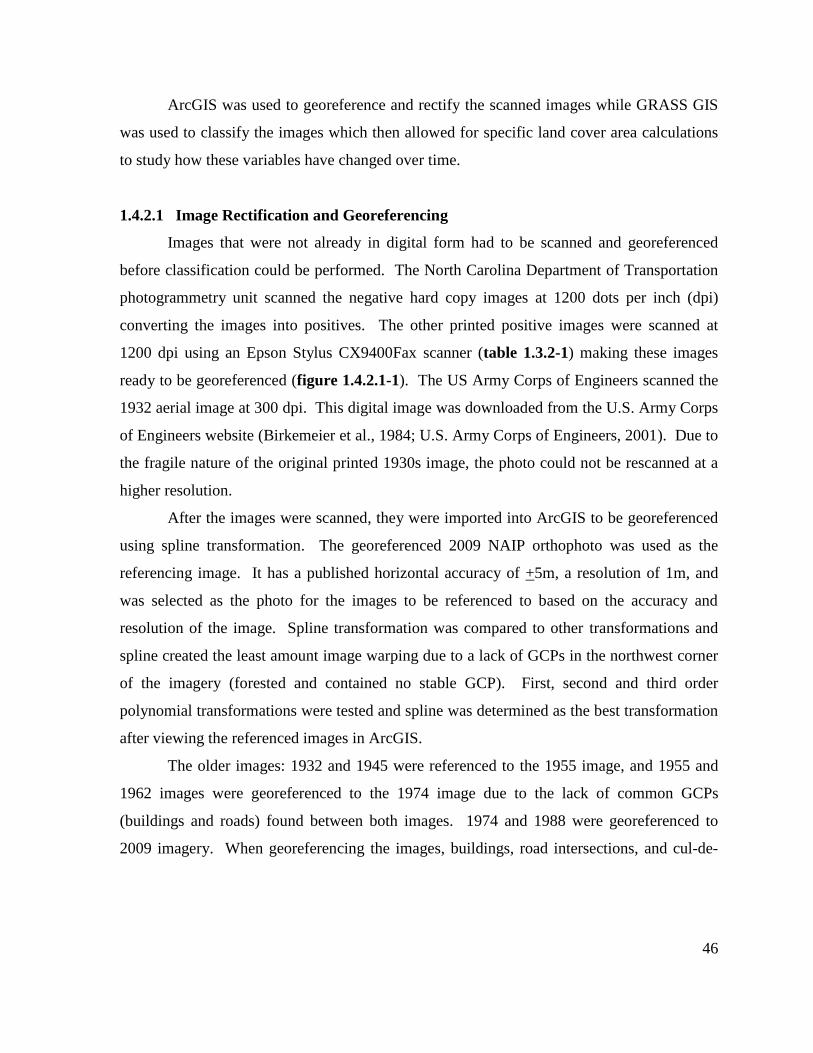
46

ArcGIS was used to georeference and rectify the scanned images while GRASS GIS

was used to classify the images which then allowed for specific land cover area calculations

to study how these variables have changed over time.


Images that were not already in digital form had to be scanned and georeferenced

before classification could be performed. The North Carolina Department of Transportation

photogrammetry unit scanned the negative hard copy images at 1200 dots per inch (dpi)

converting the images into positives. The other printed positive images were scanned at

1200 dpi using an Epson Stylus CX9400Fax scanner (table 1.3.2-1) making these images

ready to be georeferenced (figure 1.4.2.1-1). The US Army Corps of Engineers scanned the

1932 aerial image at 300 dpi. This digital image was downloaded from the U.S. Army Corps

of Engineers website (Birkemeier et al., 1984; U.S. Army Corps of Engineers, 2001). Due to

the fragile nature of the original printed 1930s image, the photo could not be rescanned at a

higher resolution.

After the images were scanned, they were imported into ArcGIS to be georeferenced

using spline transformation. The georeferenced 2009 NAIP orthophoto was used as the

referencing image. It has a published horizontal accuracy of +5m, a resolution of 1m, and

was selected as the photo for the images to be referenced to based on the accuracy and

resolution of the image. Spline transformation was compared to other transformations and

spline created the least amount image warping due to a lack of GCPs in the northwest corner

of the imagery (forested and contained no stable GCP). First, second and third order

polynomial transformations were tested and spline was determined as the best transformation

after viewing the referenced images in ArcGIS.

The older images: 1932 and 1945 were referenced to the 1955 image, and 1955 and

1962 images were georeferenced to the 1974 image due to the lack of common GCPs

(buildings and roads) found between both images. 1974 and 1988 were georeferenced to

2009 imagery. When georeferencing the images, buildings, road intersections, and cul-de-

47

sacs were chosen as GCPs due to their static nature throughout time allowing for a reliable

reference control point (figure 1.4.2.1-2). When choosing the GCPs, the center of the

structure was referenced to account for any additions/removals of buildings, or roads. 22

ground control points were selected on the 2009 photo that could also be found on the

scanned images, however, the 1932 image only allowed for 10-12 GCPs to be identified due

to a lack of homes and roads that could be used as GCPs (table 1.4.2.1-1). This image was

used as an early baseline comparison of how variables have evolved over time and was

utilized to quantitatively estimate a starting area of variables due to the uncertainty in

referencing.

Figure 1.4.2.1- 1: Due to the time scale of this study, a variety of images were used in

classification ranging from black and white historical photographs to colored infrared, for

example: (a) U.S Army Corps of Engineers printed 1932 black and white photograph, (b)

1945 negative film scanned to a positive image, (c) 1955 hardcopies of black and white

image that were scanned and (d) 2009 NAIP’s infrared orthophoto.

48

Table 1.4.2.1- 1: Ground Control Points used to georeference images to 2009 NAIP

orthophoto Decade Number of Ground Control Points and Spline Error

1930s 12 GCPs, Bottom Photograph/ 10 GCPs, Top Photograph

(Georeferencing Estimation)

1940s 22 GCPs, Top Photograph

1950s 22 GCPs, Top Photograph

1960s 22 GCPs, Bottom Photograph / 22 GCPs, Top Photograph



1990s Orthophoto

2000s Orthophoto

Today Orthophoto

Figure 1.4.2.1- 2: Georeferencing the 1974 image (a) to the 2009 NAIP orthophoto (b) using

22 ground control points (c).

49

1.4.2.2 Image Classification

The images used in this study were collected via optical remote sensing. The pixels

that compose the image reflect the sun’s radiation reflected from the earth’s surface

(Lindgren 1985; Neteler and Mitasova, 2008). Optical remote sensing techniques span the

visible (VIS, 0.4 to 0.7µm) and infrared (IR, near IR: 0.7 to 1.3µm, mid IR: 1.3 to 3µm,

thermal IR 3 to 14µm) spectrum (Lillesand et al., 2004). Image pixels contain special

signatures that can be classified or assigned to objects/materials on earth’s surface. For

example vegetation, buildings, and sand have a specific spectral signature and image pixels

can be classified into land cover based off the amount of radiation that reflects off their

surfaces. Reflectance of the sun’s energy is a result of the material, surface, vegetation, and

mineral composition that the energy comes in contact with (Neteler and Mitasova, 2008;

Richards and Jia, 2006).

Georeferenced images were masked to include the Jockey’s Ridge Park (figure 1.2-

1b) and area just north of the dune system in order to quantitatively and qualitatively capture

vegetation and development changes. The images were separated into 3 bands (Red, Green,

Blue: R,G,B) for all imagery except for the 2009 infrared which was imported as 4 bands

(R,G,B and IR bands) and 1998 imagery which contained the infrared band as one of the 3

bands. These were imported into GRASS GIS in order to classify and extract sand and

vegetation for each year of imagery. Development (roads and buildings) were digitized in

ArcGIS for each image to avoid development being classified as vegetation due to similarity

in spectral response.

Images were classified in GRASS GIS using unsupervised classification. Ten classes

were empirically selected in order to classify vegetation and sand after testing different

classes and their ability to classify these land cover types (appendix F). Selecting less than

ten classes did not accurately classify these variables and creating classes greater than ten did

not change classification results from the ten classes.

The images were imported into the image processing tools after roads and buildings

were masked out in order to only classify vegetation and sand. Unsupervised classification

50

was based on similar spectral vectors by grouping the image pixels into natural clusters

called spectral classes by statistical methods (Lillesand et al., 2004; Neteler and Mitasova,

2008). Spectral vectors are defined as the pixels at a specific location from R, G, B or IR

bands (Neteler and Mitasova, 2008). In the fully automated unsupervised classification

method, this spectral vector is matched or clustered with other spectral vectors that contain

the same or similar reflectance signatures and can be grouped in classes that represent

vegetation, sand, etc. based on image statistics: cluster mean and covariance matrices

(Neteler and Mitasova, 2008). Maximum likelihood classifier (MLC) was used as the

classifier algorithm to classify vegetation and sand for each pixel throughout the time series

of images. MLC assigns a class to each pixel with the highest probability while

simultaneously running a Chi-squared test until a convergence that was preset is obtained

producing a raster image containing pixels assigned to the number of classes predefined, in

our case ten (Neteler and Mitasova, 2008). Since this classification is automatic, the

algorithm does not know what class is assigned vegetation or sand, so classes were visually

selected by the user using the imagery to select which class corresponds to the specific land

cover (Table 1.4.2.2-1). Areas were calculated for each land cover (sand, vegetation and

development) to determine the change of variables for each year of imagery.

Table 1.4.2.2- 1: Land cover classes (vegetation and sand) visually selected from imagery

Year Vegetation Classes Sand Classes

1932 1,2,3 4,5,6,7,8,9,10

1945 1,2,3,4 5,6,7,8,9,10

1955 1,2,3,4 5,6,7,8,9,10

1962 1,2,3,4 5,6,7,8,9,10

1974 1,2,3,4 5,6,7,8,9,10

1988 1,2,3,4 5,6,7,8,9,10

1998 1,2,3,4,6 5, 7,8,9,10

2007 1,2,3,4,5,6 7,8,9,10

2009 1,2,3,4,5 6,7,8,910

51

1.5 Results

By coupling elevation data with image processing, the evolution of Jockey’s Ridge

since 2001 and the effects of the vegetation and development on geomorphology of the dune

system have been quantified. Overall, results have shown long term decreases of dune

heights and increases of vegetation and development area as well as a recent stabilization of

dune peak elevations, and the slowing down of vegetation and development expansion.

1.5.1 Geomorphic Evolution

1.5.1.1 Dune System Evolution

Animations created with high resolution elevation data of Jockey’s Ridge have

provided a dynamic visual representation of the dune field evolution over the past 36 years.

The “Aerial View of Jockey’s Ridge” (Weaver K., 2011a) and “Soundside View of Jockey’s

Ridge” (Weaver K., 2011b) animations capture the geomorphology of the dunes. For

instance, one can identify the dominant southern migration of the dune field, the deflation of

the dune peaks, and eventually, the stabilization of the dune field. The “Jockey’s Ridge Slip

Faces” (Weaver K., 2011c) animation shows the geomorphic transformation of the dune field

from coalesced barchan to coalesced parabolic dunes as well as the southern migration of the

dune field. These animations serve as a basis for the detailed quantitative analysis of

Jockey’s Ridge and are great visualization tools and reference for the evolutionary history of

this dune system.


Previous studies indicated that this large active dune evolved over a relatively short

time period, with the Main Dune rapidly growing from the early 1900s-1953 (Feltner 1948)

and steadily losing elevation from 42.10m to 24.17m between 1953-1998.

Analysis performed in this study confirms an overall decrease of dune peak heights

since 1953, but a recent increase in elevation for all of the dunes since 2007 has been

observed. Figure 1.5.1.2-1 shows the southern migration and decrease in elevation using the

52

2008 DEM with 2009 orthophoto overlaid with a time series of 3D extracted dune peaks

since 1974. The vertical lines under the labeled peaks indicate how the corresponding peak

has evolved until 2008 (increased or lost elevation). Historical elevations extracted from

profiles (Feltner 1948) and topographical maps yielded elevations dating back to 1917

revealing elevations of the Main Dune reaching peak heights of 20m in 1917 and 42m in

1953. The peaks of each dune were tracked and analyzed from 1974 to 2008 (table 1.5.1.2-

1) for all the dunes of Jockey’s Ridge. Data before 1974, contained peaks for the Main Dune

only, not permitting a complete analysis of the dune system.

Visual comparison of each of the dune’s extracted peaks (figure 1.5.1.2-2) as well as

the calculated rates of change (figure 1.5.1.2-3) confirm the predetermined overall decrease

in the heights of all dunes since 1974 with the majority of the dunes decreasing from 1953 to

1998. However, East Dune 1 and West Dune 1, which border the Main Dune, have increased

from 1998 to 2008 as well as shown similar growth/deflation trends (table 1.5.1.2-2)

indicating similar evolutional characteristics. Even though Jockey’s Ridge has lost

considerable elevation since 1953, the dunes are showing signs of rebound since 1998 for

East and West Dune 1 while the Main Dune and East 2 Dune have increased since 2007

(figure 1.5.1.2-2).

The Main Dune as well as East Dune 2 peak elevations have been decreasing at the

linear rates of 0.36m/year and 0.18m/year respectively. The rest of the dunes have decreased

from 1974-1998 at variable rates of 0.01m/year to 0.17m/year; since 1999 they have been

increasing in elevation at variable rates of 0.05m/year to 0.15m/year (figure 1.5.1.2-3). The

Main Dune as of 2004 was the highest dune as stated by Mitasova et al. (2005a), but as of

2007 West Dune 1 became the tallest dune with a peak elevation of 21.55m while the Main

Dune’s elevation was 20.8m.

East Dune 2 and the Main Dune display linear elevation decreases throughout the

study period which allowed for a linear equation to be calculated for the peak elevations with

a correlation coefficient of 0.96 and 0.98 respectively. Rates of change between years for all

53

dunes were calculated to determine how the growth of the dunes changed from year to year

(figure 1.5.1.2-3).

Figure 1.5.1.2- 1: 2009 Orthophoto draped over 2008 DEM with 1953-2008 time series of

3D peaks indicating dune peak migration.

Table 1.5.1.2- 1: Evolution of Jockey’s Ridge dune peak elevations from 1917-2008 Year 1917 1928 1931 1935 1953

Dune

West 2 --

West 1 --

Main 20.12 32.00 30.00 31.00 42.1

East 1 --

East 2 --

Year 1974 1995 1998 1999 2001 2002 2004 2007 2008

Dune

West 2 20.61 20.18 20.42 20.38 20.59 -- -- 20.72 20.96

West 1 23.91 20.13 19.80 21.18 21.41 -- -- 21.55 22.36

Main 33.53 26.04 24.17 26.43 25.06 23.63 21.92 20.81 21.56

East 1 20.22 16.81 16.75 17.72 18.04 -- -- 18.33 19.60

East 2 21.05 16.81 15.68 16.21 15.43 -- -- 14.85 15.22

West 2 Dune West 1 Dune Main Dune East 1 Dune East 2 Dune

54

1970 1975 1980 1985 1990 1995 2000 2005 201014

16

18

20

22

24

26

28

30

32

34The Evolution of Jockeys Ridge Dune Peaks From 1950 to 2008

Year

Ele

vation (

mete

rs)

East 1 Dune

East 2 Dune

Main Dune

West 1 Dune

West 2 Dune

Figure 1.5.1.2- 2: The evolution of Jockey’s Ridge dune peak elevations from 1974 to 2008.

LiDAR Extracted Dune Peaks

55

Figure 1.5.1.2- 3: Rates of change in peak elevations: Individual dune peak elevation graphs

showing rates of change approximated by linear regressions. Linear regressions were

calculated for East Dune 2 and the Main Dune while two linear regressions were calculated

for East Dune 1, and West Dune 1 and 2, between 1974 and 1998 and between 1999 and

2008.

Table 1.5.1.2- 2: Similar vertical rates of change for East Dune 1 and West Dune 1

1974 - 1995 1995 - 1998 1998 - 1999 1999 - 2001 2001 - 2007 2007 - 2008

East 1 -0.16 m/yr -0.02 m/yr 0.97 m/yr 0.16 m/yr 0.05 m/yr 1.27 m/yr

West 1 -0.18 m/yr -0.11 m/yr 1.38 m/yr 0.12 m/yr 0.02 m/yr 0.81 m/yr

1.5.1.3 Horizontal Migration

The southerly migration of Jockey’s Ridge was analyzed using several geospatial

techniques including visualization of dune field cross sections. Quantification of horizontal

dune migration rates was performed using dune crests and peaks.

y=-0.1511x+318.5448 R2 = 0.99

y=0.1548x+-291.6898 R2 = 0.69

y=-0.1745x+368.3082 R2 = 0.998

y=0.0951x+-168.8591 R2 = 0.67

y=-0.0125x+45.3531 R2 = 0.58

y=0.0509x+-81.4009 R2 = 0.86

y=-0.1828x+381.5630 R2 = 0.96

y=-0.3583x+740.9430 R2 = 0.98

56

Visualizing Dune Migration Simultaneous perspective view of overlaid 2001 and 2008’s

DEMs (figure 1.4.1.4-2) and cross sections generated by cutting planes confirms the dune’s

southerly migration and the deflation of the dune peaks between these two years. These

DEMs were selected in order to analyze how the dune has evolved since the study conducted

by Mitasova et al. 2005a. The cross sections show sand that has been eroded from the

northern windward side and deposited on the southern leeward side of dune as sand is being

transported over the dune and down the slip face causing the dune to migrate south.

2001 and 2007 DEMs were differenced in order to map the change since Mitasova et

al., 2005a’s study. 2007 was chosen due to it being the most recent data set since removal of

the South Dune. Southern migration of the dune was detected by analyzing areas that had

deposition or erosion of sand. Figure 1.5.1.3-1 indicates areas where sand was eroded

(northern windward side of the dune) and deposited (southern leeward side of the dune). In

addition to south migration, the difference map shows deposition along the eastern side of the

Main Dune and a small western “finger like” dune evolving along the southern part of the

Main Dune (figure 1.5.1.3-1) due to changing wind directions.

Graphing extracted dune peaks (figure 1.5.1.3-2) and dune crests (figure 1.4.1.3-3)

for each dune of the time series confirmed the migration of these features.

Quantifying Dune Migration Mitasova et al. (2005a) calculated Jockey’s Ridge to be

migrating south 3m-6m a year based on change in the dune crests position. Independent

analysis of dune crests migration that included new LiDAR DEMs (2007 and 2008) found

the entire dune system to be migrating south on average 3.7m/year. The East Dune

(combination of East 1 and East 2 Dunes) was migrating south the fastest at a rate of

5.26m/year migrating a distance of 178.73m since 1974. The Main Dune which was

migrating the slowest, with the eastern slip face migrating at 3.02m/year (102.71m distance),

Main Dune west “finger” migrating at 3.26m/year (110.90m distance) and the south face

migrating a 3.56m/year (distance of 121.00m). The southern face of the West Dune was

found to be migrating at 3.58m/year a distance of 121.70m (figure 1.5.1.3-3, Appendix H).

57

Individual migration rates for the time series of DEMs were calculated for all dunes and are

shown in Appendix H.

Dune peaks demonstrated a similar pattern of horizontal migration as found by the

dune crests. Horizontal migration rates were calculated for all the dunes (Appendix I).

Figure 1.5.1.3-4 shows the horizontal rates of peak migration along a cumulative path

ranging between 4m/year to 9m/year. East Dune 2 peak has overall migrated the farthest

with a rate of 8.72m/year with West Dune 2 migrating at 8.66m/year. The Main Dune peak

moved the shortest distance with a rate of 4.21m/year. As found in the vertical rates of

change, East Dune 1 and West Dune 1 display similar horizontal evolutionary patterns, East

Dune 1 has migrated a total of 217m with a rate of 6.4m/year while West Dune 1 has

migrated a total distance of 233m with a migration rate of 6.86m/year.

The migration of the dune peaks is complex, migrating in different directions

dependent upon peak location along a longer path than the dune crests. Due to the nature of

the dune peak to migrate in different directions, the distance is measured cumulatively from

1974 to each peak and covering a longer distance making a higher migration rate for the

peaks. By comparing dune crests to dune peaks, similar patterns of migration are apparent.

Even though dune crests migrate at slower rates, similar trends for migration rates are found

with crests and peaks. The Main Dune’s crests and peaks are migrating the slowest and the

East Dune’s crests and peaks are migrating the fastest.

Distance was also measured from each dune’s 1974 peak to the 2008 peak using a

straight path (not cumulative distances). It was found that East Dune 1 migrated 216.15m

with a horizontal migration rate of 6.36m/year, East Dune 2 migrated 147.72m at a rate of

4.34m/year, the Main Dune traveled 94.21m at a rate of 2.77m/year, West Dune 1 traveled

144.07m at a rate of 4.24m/year while West Dune 2 migrated 158.42m at a rate of

4.66m/year. This methodology is similar to how dune crest migration rates were calculated.

These results were compared to dune crests migration rates, yielding similar results. The

Main Dune peaks and crests traveled the slowest and migrated the shortest distance while the

58

East Dune peaks and crests traveled the fastest and migrated the farthest during the study

period.

Figure 1.5.1.3- 1: Difference Rasters: (a) between 2001 and 2007 multiple return DEMs and

(b) 2007 and 2008 multiple return DEMs showing southern and eastern migration of dune

indicated by the addition of sand on the southern leeward and eastern leeward side of the

dunes (blue). Note South Dune’s difference elevation is red indicating a removal of sand

(green oval) and addition of sand north of the Main Dune in 2003 (green arrows). Areas of

blue indicate sand addition and areas of red represent erosion of sand.

Sand Gain

Sand Loss

59

Figure 1.5.1.3- 2: Aerial view of time series of dune peak locations

60

Figure 1.5.1.3- 3: Horizontal migration of dune crests from 1974 to 2008

Figure 1.5.1.3- 4: Horizontal dune peak migration measured from 1974.

61

1.5.1.4 Volume Change and South Dune’s Relocation

Volume Change The volume of sand above 6m elevation was found to remain relatively

consistent, fluctuating around the average volume of 4.99x106m

3. The volume ranged

between 5.147x106m

3 and 4.607x10

6m

3 from 1974 until 2008 with a minimum volume in

1998 and a recovery to near average volumes in 1999 (figure 1.5.1.4-1). As of 2008 the

active portion of Jockey’s Ridge dune had a volume 5.04x106m

3 of sand.

South Dune’s Status One of the main goals of relocating the South Dune north of the Main

Dune, was to “feed” the deflating Main Dune. Unfortunately, since the 2003’s South Dune

removal a LiDAR flight was not flown until 2007. The only data sets available since the

removal are 2007 and 2008, however, there was a LiDAR flight in 2001 allowing for before

and after analysis.

Figure 1.5.1.3-1, a difference map between 2001 and 2007 multiple return (MR)

shows the removal of the South Dune and relocation of the sand just north of the Main Dune.

A difference map between 2007MR and 2008 yielded almost no change in elevation for the

relocation area indicating that the disposal sand has already been redistributed. Jennifer Cox,

a Jockey’s Ridge Park Ranger confirmed that the sand relocated from the South Dune is no

longer in the disposal location and coarse debris that wind could not transport have settled

while the finer sand has been transported away by aeolian processes (figure 1.1-3d; Cox,

personal communication).

Due to the limited data after 2003, it was not possible to accurately trace the sand

transport from the disposal area and assess whether it has contributed to the observed

increase in dune peak elevations.

62

Figure 1.5.1.4- 1: Total volume of sand in the active area of Jockey’s Ridge dune system.


Time series of elevation data made it possible to extract core (2,088,147.8m3) and

envelope surfaces. The volume of dynamic sand (Equation 12) for each year remained

around a mean value of 2,905,578m3 fluctuating between 2,518,447m

3 to 3,058,957m

3

(Table 1.5.1.5-1). Figure 1.5.1.5-1 shows the graphed volumes of the dynamic layer

indicating a relatively constant volume of dynamic sand throughout the time series with the

exception of 1998. Calculation of the relative volume revealed an average ratio of 0.47

(table 1.5.1.5-1) indicating that there was no single year when the entire dune’s elevation

(surface) was at a minimum or maximum (figure 1.5.1.5-2).

63

Table 1.5.1.5- 1: Volumes of dynamic sand and relative volumes extracted from core and

envelope using time series of data

Year Volume

(m3) Volume of Dynamic

Sand (m3) Relative Volume

(Ri) Core Volume

(m3) Envelope

Volume (m3)

1974 5121400 3033252 0.492 2088148 8256462

1995 5089873 3001725 0.487 1998 4606595 2518447 0.408 1999 5147105 3058957 0.496 2001 5100113 3011965 0.488 2007 4855767 2767619 0.449 2008 5035230 2947083 0.478

Figure 1.5.1.5- 1: Volume of dynamic sand (volume of DEM above 6m elevation-volume of

core) from 1974 to 2008.

64

Figure 1.5.1.5- 2: Relative volume expressed between 1 (envelope) and 0 (core). Volume

extracted above 6m elevation yields relative volumes around 0.5 indicating that sand is not

entering or leaving the system, however the sand is being redistributed amongst the dunes

(Graph created by Eric Hardin from North Carolina State University).


The Outer Banks and more specifically the Jockey’s Ridge study area have undergone

dramatic land cover changes since the 1930s as shown in the “Jockey’s Ridge Aerial

Imagery” animation (Weaver K., 2011d). The analysis of imagery confirms that the 1930s

was a period of no development or vegetation growth. Overtime vegetation and development

increased while the total area of sand decreased. Image classification (figure 1.3.2-1) using

three land covers: sand, vegetation and development (figure 1.5.2-1, table 1.5.2-1) shows

that 1932 had the largest area of sand totaling 80.98% of the total study area (295ha), while

vegetation only covered 18.61% of study area with development (road along present day

Highway 12) accounting for the 0.41% of the remaining area. As of 2009 the area of sand

had decreased by half to 46.14% coverage while vegetation had doubled to 42.52% and

development increased to 11.34%.

65

Coupling DEMs with land cover extracted from imagery, visualization of topography

and land cover can be helpful to assess the spatial relationship between the land cover change

and evolution of topography (figure 1.5.2-2). The overall change of the dynamic land cover

can be viewed in the “Jockey’s Ridge Imagery Classification” animation (Weaver K.,

2011e).

Linear regressions were calculated for sand, development and vegetation areas

throughout the time series yielding a linear change: development: y=0.46x-888.84 providing

an R2 of 0.96, sand: y=-1.349x+2.847e+03 with an R

2 of 0.96 and finally vegetation:

y=0.836x-1.553e+03 giving an R2 of 0.96. Figure 1.5.2-3 displays the variables plotted with

corresponding linear regressions and R2 values. The overall trend of the data indicates that

the area of sand was at a maximum in 1932 (decreasing at a rate of 1.35ha/year) and has

steadily decreased to a minimum in 2009 while development (increasing at a rate of

0.46ha/year) and vegetation (increasing the fastest at a rate of 0.84ha/year) and have both

increased overtime.

66

1932 1945 1955

1962 1974 1988

1998 2007 2009

Figure 1.5.2- 1: Classified Imagery with % area of sand (S-grey), vegetation (V-green) and

development (D-red).

80.98% S

18.61% V

0.41% D

74.51% S

24.63% V

0.86% D

71.93% S

26.51% V

1.56% D

63.21% S

34.55% V

2.24% D

64.13% S

30.75% V

5.12% D

55.83% S

35.98% V

8.19% D

47.47% S

43.76% V

8.77% D

50.31% S

38.76% V

10.93% D

46.14% S

42.52% V

11.34% D

67

Table 1.5.2- 1: Land cover areas calculated from classification of sand, vegetation and

development using aerial photographs (1932 to 2009)

Year Sand (ha) Vegetation (ha) Development (ha)

1932 245.7855 56.4951 1.2373

1945 219.7477 72.6299 2.5383

1955 212.2196 78.2197 4.6136

1962 186.5939 101.995 6.6044

1974 189.3041 90.7825 15.107

1988 164.8040 106.2094 24.1823

1998 140.1310 129.1722 25.8923

2007 148.5218 114.4096 32.2665

2009 136.2018 125.5091 33.4832

Figure 1.5.2- 2: 2007 LiDAR DEM overlaid with 2007’s aerial photograph classification of

sand, development and vegetation land cover map obtained by classification of aerial

orthophoto.

68

Figure 1.5.2- 3: Time series of classified land cover (sand, vegetation and development)

with linear regressions

1.6 Discussion

By combining historical elevation data with high resolution LiDAR and imagery, a

detailed geospatial analysis of the morphology and land cover of Jockey’s Ridge dune system

has yielded results that have aided in the understanding of this complex dune system.

Even though elevation data sets that cover Jockey’s Ridge are limited; the time series

of DEMs that are available were sufficient for quantitative analysis and visualization of dune

morphology evolution. There is a large collection of imagery available for the Outer Banks

that permitted the investigation of the relationship between land cover change and the

morphology of Jockey’s Ridge. With the combination of both data sets an overall detailed

69

analysis of the evolution of Jockey’s Ridge yielded new results as well as confirmed past

findings.

As concluded in the previous studies (Havholm et al., 2004; Judge et al., 2000;

Mitasova et al., 2005a; Pelletier et al., 2009; Runyan and Dolan 2001), the Jockey’s Ridge

area has undergone a morphological change since its formation about 1,200 years ago.

Between 1917 and 1953 the dune grew to a maximum peak height of 42m and steadily

decreased in elevation by almost half to 22m between 1953 and 2008. Over time the dune

system evolved from a single dune into five well defined dunes with peaks, ridges, slip faces

and relatively similar elevations. The dunes seem to be evolving from barchan dunes formed

during times of little vegetation cover, to parabolic dunes. These parabolic dunes are created

by an increase of vegetation causing the dunes to be sand starved, leading to loss of

elevation. Parabolic dunes are known for tails that follow behind the dune, pointing upwind.

Due to the coalesced form of these dunes, the tails of Jockey’s Ridge dunes are not visible

but the well defined slip faces and ridges can be detected and the time series of DEMs shows

the evolution from coalesced barchan dunes to sand starved parabolic dunes (Desert

Processes Working Group). The combination of increased vegetation and development on

the windward side of the dune field decreased the amount of sand feeding the dune, leading

to a decrease of dune height.

One of the more interesting results found in the geomorphology study was that the

West Dune 1 and East Dune 1 which are situated on the east and west sides of the Main Dune

have similar evolutionary patterns. West Dune 1 and East Dune 1 have vertically evolved at

similar rates: East Dune 1: -0.16m/year to 1.27m/year and West Dune 1: -0.18m/year to 0.81

m/year (table 1.5.1.2-2, figure 1.5.1.2-3). When measuring horizontal migration rates using

dune peaks these dunes showed similar trends (East Dune 1: 6.4m/year and West Dune 1:

6.86m/year; figure 1.5.1.3-4). It is hypothesized since the Jockey’s Ridge dune field itself is

dynamically evolving and forming five well defined parabolic dunes and the increase of

vegetation and development is causing aeolian sand transport to decrease. The sand that is

already part of Jockey’s Ridge is being redistributed and spread out (deflation of dune peaks)

70

and the sand that was once part of the high Main Dune in 1953 may be contributing to the

growth of the East Dune 1 indicated by the southern migration and clockwise rotation of the

dunes.

One additional surprising result from the geomorphology study is that the “Main

Dune” which stood 42m in 1953 is no longer the highest dune of Jockey’s Ridge. Examining

1932’s topographic map, the dune once called “Engagement Hill,” today is referred to as the

Main Dune was the only recorded dune in 1917 and has been recorded as the highest dune

until 2007. As of 2007, West Dune 1 became the highest dune of Jockey’s Ridge with a

height of 21.55m while the Main Dune’s elevation was 20.8m. As of 2008 West Dune 1

grew to 22.36m while the Main Dune grew to 21.56m, but was still lower then West Dune 1.

Due to the large gap between LiDAR data collections of 2001 and 2007, West Dune 1 could

have been taller than the Main Dune before 2007, however due to the time interval of data

collections it is safe to conclude that the Main Dune as of 2007 is no longer the tallest dune

of Jockey’s Ridge. It is hypothesized that the migration and reworking of the Main Dune

into smaller dunes has transferred the sand to West Dune 1 causing West Dune 1 to have a

higher dune peak.

As for the fate of the South Dune’s relocation, with the data available to us, it is

difficult to determine how this relocation windward of the dune field has contributed to the

Main Dune’s growth. Due to the prevailing northeastern winds, it is safe to assume that the

sand from the relocated South Dune has in some form added to elevation of the dune field,

not just to the Main Dune but to other dunes as well.

One promising result is that even though the dunes have lost significant elevation, as

of 2007 all dunes are showing signs of growth with rates between (0.24m/year to 1.27m/year)

and as of 2008 the dunes seem to be reaching stable elevations between 15m and 22m with

an average peak height of 20m. The volume of sand within Jockey’s Ridge seems to remain

within the park boundaries (with a negligible volume of sand escaping onto Highway 158 at

times) remaining around the average volume of 4.99x106m

3. This is evident based on core

and envelope analysis, and calculations of yearly dynamic sand and relative volume rates. It

71

was found that Jockey’s Ridge dune field has a stable core volume of 2,088,147m3. Since

the volume of dynamic sand fluctuates around the average value of 2,905,578m3 and contains

an average relative volume of 0.47, this leads us to believe that the sands of Jockey’s Ridge

are being reworked by wind and redistributed amongst the dunes and not gaining or losing

sand into its system. Most of the active sand that was present in 1974 seems to be present

today, confirming that Jockey’s Ridge has not lost volume but redistributed its sand

elsewhere around the dune system.

Not only has vegetation change been attributed to dune stabilization around the North

Carolina Outer Banks, but loss of sand sources from increased development has also affected

the growth of the dunes. Development and vegetation have reduced areas of available sand,

decreasing sand transport that once fed the Jockey’s Ridge dunes. Buckley (1987) found that

as vegetation increased, sand transport decreased which has been observed in the Jockey’s

Ridge area as indicated by the stabilization of the dunes. Havholm et al. (2004)’s research

suggests that we are approaching a phase of stabilization and revegetation. Using our

selected study area, 1932 was a time of almost no vegetation or development allowing the

dune to be in an active barchan stage. Vegetation and development increased throughout the

study time period and as of 2009 vegetation covered almost half of our study area, which was

associated with a loss of half the dune peak elevation since 1953.

The majority of the vegetation and development change occurred on the windward

side of the dune field, which was the primary source of sand feeding the dunes as stated by

Runyan and Dolan (2001). If the source is being covered by vegetation and development, the

sand is being trapped and the source is no longer active and feeding the dunes. A

combination of vegetation and development increasing on the windward side of the dune

field would account for the deflation of Jockey’s Ridge due to sand transport decreasing due

to vegetation and buildings detaining the sand. This analysis indicates that overall vegetation

has covered a larger area and grown faster than development. Over time development has

replaced vegetation rather than sand. Within the park boundaries, and along the dunes

vegetation has been increasingly taking over, figure 1.6-1 shows vegetation climbing over

72

the slip face of the Main Dune from a visit in March, 2010 and a visit in July, 2010

illustrating the increase of vegetation. Graphing dune peaks with area of land cover, it is

evident that as vegetation and development increase, the Main Dune lost peak elevations

(figure 1.6-4) as well as East Dune 2 (figure 1.6-3b). The other dunes do not seem to be

affected due to the increase of vegetation and development, however are affected due to the

redistribution of sand from the Main Dune which may be contributing to their elevations

(figure 1.6-2, figure 1.6-3a).

Modeling efforts by Pelletier et al., 2009 show similar results using dune field

evolution modeling. Simulations were ran studying dune formation with the introduction of

interdune vegetation using Jockey’s Ridge as a case study. Results indicated that with the

presence of vegetation, dune elevations decreased and conversely without vegetation, dunes

were able to grow. Using dune modeling Pelletier et al. (2009) was also able to conclude that

the reworking of sand within the dune system is the result of vegetation growth within the

dune system however this study adds in development.

Jockey’s Ridge is not only affected by increases of vegetation and development, but

due to its location is affected by intense hurricanes and winter storms (Nor’easters) which

help redistribute the sand and affect dune evolution. Hirsch et al. (2001) describes East

Coast Winter Storms (ECWS) as being comparable to hurricanes in regards to storm damage

in coastal areas. Hirsch et al. (2001) found that each winter season (October to April), on

average twelve ECWS occur with maximum winds reaching about 46mph, and maximum

ECWS happening in January. Hurricanes and tropical storms occurring between June and

November along the North Carolina coast on the other hand happen less frequently than

ECWS; figure 1.6-5 shows the decadal breakdown of hurricanes (category 1 to category 5)

and tropical storms that have affected North Carolina. Averages based off these results

indicated a yearly average of 2.24 storms affecting North Carolina, which is significantly less

than the amount of ECWS in this area (State Climate Office of North Carolina, b). Using

North Carolina State Climate Office’s hurricane archives between 1932 to 2009, 4 category 4

hurricanes, 13 category 3 hurricanes, 27 category 2 hurricanes, 38 category 1 hurricanes and

73

79 tropical storms affected North Carolina (State Climate Office of North Carolina, b).

Weaker storms (category 1 and tropical storm) are significantly more frequent than more

intense hurricanes, ruling out hurricanes as being the driving force of overall dune migration.

When comparing hurricane frequency and strength with ECWS frequency and strength, the

effects of the Nor’easters coupled with dominate northeasterly winds are climatic influences

on the southern migration indicated by Havholm et al. 2004’s sand transport rose (figure 1b

in Havholm et al. 2004).

Future Work Due to time constraints, ground truth accuracy assessment of image

rectification and classification of imagery was not performed in this study. However,

GRASS GIS module i.maxlik outputs a raster that contains confidence levels in each of the

pixels. These confidence levels state how confident each pixel was assigned to a specific

class (Neteler and Mitasova, 2008). Figure 1.6-6 and figure 1.6-7 show the histogram of

confidence intervals for 1974 and 2009 classified imagery. Each classified image in the time

series has similar confidence level histograms results. Classification results obtained from

this study were visually checked using 3D viewers, imagery and DEMs. In order to

quantitatively assess the accuracy of image rectification, GCPs will be selected and used to

estimate accuracy. Then classification errors will be calculated for the unsupervised

classification methodology by selecting areas that are known to be vegetation and sand

around the Jockey’s Ridge area evaluating the accuracy of land cover classification for the

time series of imagery.

The 1998 DEM needs to be investigated due to decreases in DEM derived data such

as rapid decreases in dune peak elevations and volumes. Point density may be one factor

causing the decreases in values throughout this study. The 1998 DEM contained a less dense

point cloud (figure 1.3.1-2f) compared to other DEMs used in this study. It is hypothesized

that a decrease in point density changes the shape of topography as well as other terrain

features such as dune peaks (if missed when collecting photogrammetric mass points) as well

as decreases in volume due to points not capturing the terrain’s complete geometry.

74

In order to investigate the driving force of the evolution of Jockey’s Ridge and dunes

along the eastern coast of North Carolina, a climatological study needs to be completed in

order to further this study and relate the dune’s evolution to climatological events. For

example, hurricanes/tropical storms and Nor’easters correlated with specific dune deflation

and dune growth events would be pertinent in order to understand the dune’s evolution on a

climatic time scale.

Lastly, it would be interesting to apply these techniques to other coastal dunes around

the world to investigate whether there is a global pattern of cyclical changes of vegetation

growth and if development plays a role in the morphology of other dune systems.

Figure 1.6- 1: Vegetation crawling over Main Dune’s slip face between March and July

2010.

75

a.

b.

Figure 1.6- 2: Relating land cover change to (a) West Dune 2 and (b) West Dune 1 elevation

change by combining classification areas extracted from imagery and dune peak elevations.

--- Classification Areas Dune Peak Elevations

76

a.

b.

Figure 1.6- 3: Relating land cover change to (a) East Dune 1 and (b) East Dune 2 elevation

change by combining classification areas extracted from imagery and dune peak elevations.


77

Figure 1.6- 4: Relating land cover change to Main Dune elevation change by combining

classification areas extracted from imagery and dune peak elevations.

Figure 1.6- 5: Total storms (tropical storms and hurricanes) affecting North Carolina by

decade (1932 to 2009). (Image courtesy of State Climate Office of North Carolina, b)


78

Figure 1.6- 6: (a) 1974 Imagery classification (d) histogram of (c) maximum rejection

output (from GRASS GIS module i.maxlik) indicating confidence of pixels being classified to

a certain class (b).

79

Figure 1.6- 7: (a) 2009 Imagery classification (d) histogram of (c) maximum rejection

output (from GRASS GIS module i.maxlik ) indicating confidence of pixels being classified to

a certain class (b).

1.7 Conclusions

By coupling historical data with recent LiDAR data and imagery, a geospatial

analysis of the morphology of Jockey’s Ridge was investigated. While previous conclusions

were confirmed, new and surprising results were found relating to the dune’s morphology

such as the quantification of land cover.

Since the last data collection by RTK-GPS in 2004 (Mitasova et al., 2005a), the

continuation of southern horizontal migration of the dune field has been confirmed. By

80

measuring horizontal migration using the dune crests and dune peaks, each dune

demonstrates an overall southern migration trend as seen since the early formation of the

dune system. The development of additional faces to the Main Dune was also detected

demonstrating the clockwise rotation as well as southerly migration of the dune system.

However, dune peaks demonstrated a more complex pattern of horizontal migration,

cumulatively migrating along longer distances in all directions with a prevailing southerly

direction.

The overall trend since the 1930s shows, as predicted, that vegetation has

dramatically increased, along with development. Both factors seem to be playing a role in

the morphology of the dune field due to both increasing in the area that once fed the dunes.

With these increases, the once active area is being stabilized and is no longer contributing

sand to the dune’s volume. Development seems to be stabilizing since there is no longer

space for development to occur because the majority of the study area is a protected state

park or is already developed. However, vegetation is increasing inside the park boundaries

(causing the area of sand to decrease) with the majority of growth along the windward side of

the dune system as well as along the leeward side of the dune field which was predicted due

to the ongoing return to a stabilized-vegetated dune phase as Havholm et al. (2004) was able

to show. Based on our research, Jockey’s Ridge is expected to gradually change into a

vegetated stabilized dune with peak elevations reaching similar heights.

Based on evolutionary data we have studied, the dune seems to show a predicted

pattern of evolution over time. However, it is difficult to determine what the dune will look

like in the future due to many factors playing a role in its development and the dynamic

environment in which it is located. The volume of sand composing Jockey’s Ridge remains

consistent throughout time, confirming that no additional sand is entering or leaving the dune

system, but a simple reworking amongst the dunes themselves brought forth by increases of

development and vegetation. Today, dune peaks are all growing; however, the Main Dune

has lost considerable heights in elevation and another dune has taken the role of the highest

dune of Jockey’s Ridge although all the dunes seem to be reaching similar stabilized

81

elevations. Vegetation and development, if allowed to continue will ultimately cause the

dune to stabilize until climate or other factors change the environment for continued

vegetation growth.

Jockey’s Ridge has withstood this dynamic area for the past 1,200 years, and it will

continue to endure the perpetual beatings from hurricanes/storms and increases of

development and vegetation. With the promising results that Jockey’s Ridge is not loosing

sand from its system and the present day growth of dune peaks, it is safe to say that Jockey’s

Ridge will be around for many years to come.

1.8 References

Berger, G.W., Murray, A.S., Havholm, K.G., 2003. Photonic dating of Holocene back-barrier

coastal dunes, northern North Carolina, USA. Quaternary Science Reviews 22(10-

13), 1043-1050.

Birkemeier, W., Dolan, R., Fisher, N., 1984. The Evolution of a Barrier Island: 1930–1980.

Shore and Beach, 52 (2), 2 –12.

Buckley, A., Hurni, L., Kriz, K., Patterson, T., Olsenholler, J., 2004. Cartography and

visualization in mountain geomorphology. In: Bishop, M.P., Shroder, J.F. (Eds.),

Geographic Information Science and Mountain Geomorphology. Springer-Praxis,

NY, pp. 253–287.

Buckley, R., 1987. The effect of sparse vegetation on the transport of dune sand by wind.

Nature, 325, 426-428.

Cobb, C., 1906. Where the wind does the work. The National Geographic Magazine 17, 310–

317.

Coffman, Scott, 12 January, 2011. Jockey’s Ridge Ranger. Personal communication by

phone.

Cox, Jennifer, 26 January, 2011. Jockey’s Ridge Ranger. Personal communication by phone.

Desert Processes Working Group. Summary: Dunes, General. Knowledge Sciences, Inc.

http://www.agc.army.mil/desert_guide/lsmsheet/lsdune.htm (accessed 26 July, 2011).

http://www.agc.army.mil/desert_guide/lsmsheet/lsdune.htm

82

Feltner, C. E., 1948. Beach Erosion in North Carolina. The Department of Engineering

Research Bullitin No.37: North Carolina State College Record, 47(4).

Filin, S., 2005. Elimination of systematic errors from airborne laser scanning data.

Geoscience and Remote Sensing Symposium, IGARSS ’05. Proceedings. IEEE

International (Vol. 1).

Gatziolis, D., Andersen, H.-E., 2008. A Guide to LIDAR Data Acquisition and Processing

for the Forests of the Pacific Northwest ( No. PNW-GTR-768). Pacific Northwest

Research Station: United States Department of Agriculture.

http://www.fs.fed.us/pnw/pubs/pnw_gtr768.pdf

Hardin, E., Mitasova, H., and Overton, M., 2011. Quantification and characterization of

terrain evolution in the Outer Banks, NC. Proceedings of the Coastal Sediments `11,

Miami, FL. 739-753

Havholm, K.G., Ames, D.V., Whittecar, G.R., Wenell, B.A., Riggs, S.R., Jol, H.M., Berger,

G.W., Holmes, M.A., 2004. Stratigraphy of Back-Barrier Coastal Dunes, Northern

North Carolina and Southern Virginia. Journal of Coastal Research 20 (4), 980–999.

Hirsch, M. E., DeGaetano, A. T., Colucci, S. J., 2001. An East Coast Winter Storm

Climatology. Journal of Climate, 14(5), 882-899.

Horn, B.K.P., 1981. Hill shading and the reflectance map. Proceedings of the Institute of

Electrical and Electronics Engineers (IEEE), 69(1), 14–47.

Judge, E.K., Courtney, M.G., Overton, M.F., 2000. Topographic Analysis of Dune Volume

and Position, Jockey’s Ridge State Park, North Carolina. Shore and Beach, 68(4), 19–

24.

Lillesand, T. M., Kiefer, R. W., Chipman, J. W., 2004. Remote Sensing and Image

Interpretation, fifth ed. Wiley, New York.

Lindgren, D. T., 1985. Land use planning and remote sensing. Martinus Nijhoff Publishers,

Dordrecht, The Netherlands.

Mitasova, H., Hofierka, J., 1993. Interpolation by regularized spline with tension: II.

Application to terrain modeling and surface geometry analysis. Mathematical

Geology 25, 657– 669.

Mitasova, H., Mitas, L., 1993. Interpolation by regularized spline with tension: I. Theory and

implementation. Mathematical Geology, 25, 641– 655.

http://www.fs.fed.us/pnw/pubs/pnw_gtr768.pdf

83

Mitasova, H., Mitas, L., Brown, W.M., Gerdes, D.P., Kosinovsky, I., 1995. Modeling

spatially and temporally distributed phenomena: new methods and tools for GRASS

GIS. International Journal of Geographic Information Systems, 9(4), 433–446.

Mitasova, H., Overton, M., Harmon, R.S., 2005a. Geospatial analysis of a coastal sand dune

field evolution: Jockey’s Ridge, North Carolina. Geomorphology, 72, 204-221.

Mitasova, H., Mitas, L., Harmon, R.S., 2005b. Simultaneous spline interpolation and

topographic analysis for LiDAR elevation data: methods for Open source GIS. IEEE

Geoscience and Remote Sensing Letters, 2(4), 375–379.

Mitasova, H., Overton, M., Recalde, J.J., Bernstein, D., Freeman, C., 2009a. Raster-Based

Analysis of Coastal Terrain Dynamics from Multitemporal Lidar Data. Journal of

Coastal Research, 25(2), 507–514.

Mitasova, H., Hardin, E., Overton, M., Harmon, R.S., 2009b. New spatial measures of

terrain dynamics derived from time series of lidar data. Geoinformatics 17th

International Conference. Pg. 1-6.

Mitasova, H., Hardin, E., Overton, M.F., Kurum, M.O., 2010. Geospatial analysis of

vulnerable beach-foredune systems from decadal time series of lidar data. Journal of

Coastal Conservation, 14(3), 161-172.

Mitasova H., Harmon R.S,. Weaver K., Lyons, N. and Overton, M., 2011. Scientific

visualization of landscapes and landforms, Geomorphology, In Press, Corrected

Proof, Available online 13 June 2011.

National Hurricane Center. 2011. NOAA National Weather Service.

http://www.nhc.noaa.gov/ (accessed 1 July, 2011).

Neteler, M., Mitasova, H., 2008. Open Source GIS: A GRASS GIS Approach, Third edition.

Springer, NY.

NOAA Coastal Services Center. Beach Nourishment: A Guide for Local Government

Officials. http://www.csc.noaa.gov/beachnourishment/html/geo/barrier.htm (accessed

21 December, 2010).

Pelletier, J. D., Mitasova, H., Harmon, R.S., Overton, M., 2009. The effects of interdune

vegetation changes on eolian dune field evolution: a numerical‐modeling case study

at Jockey’s Ridge, North Carolina, USA. Earth Surface Processes and Landforms,

34(9), 1245-1254.

http://www.nhc.noaa.gov/

http://www.csc.noaa.gov/beachnourishment/html/geo/barrier.htm

84

Richards, J. A., Jia, X., 2006. Remote Sensing Digital Image Analysis: An Introduction,

fourth ed. Springer, Germany.

Runyan, K.B., Dolan, R., 2001. Origin of Jockey's Ridge, North Carolina: The End of the

Highest Sand Dune on the Atlantic Coast? Shore and Beach, 69, 29– 32.

Schenk, T., 2001. Modeling and Analyzing Systematic Errors in Airborne Laser Scanners.

Technical Notes in Photogrammetry No 19, The Ohio State University: Department

of Civil and Environmental Engineering and Geodetic Science.

Smith, M.J., Clark, C.D., 2005. Methods for the visualization of digital elevation models for

landform mapping. Earth Surface Processes and Landforms, 30(7), 885–900.

Starek, M.J., Mitasova, H., Hardin, E., Weaver, K., Overton, M., Harmon, R.S., 2011,

Modeling and Analysis of Landscape Evolution at Multiple Scales Using Airborne,

Terrestrial, and Laboratory Laser Scanning, Geosphere (accepted).

State Climate Office of North Carolina (a). 1971-2000 Climate Normals.

http://www.nc-climate.ncsu.edu/cronos/normals.php?station=315303 (accessed 26

July, 2011)

State Climate Office of North Carolina (b). Hurricanes-Statistics.

http://www.nc-climate.ncsu.edu/climate/hurricanes/statistics.php?state=NC (accessed

26 July, 2011).

State of North Carolina, 1976. Jockey’s Ridge Master Plan. Raleigh, North Carolina.

Stick, D., 1958, The Outer Banks of North Carolina, 1584-1958, The University of North

Carolina Press, Chapel Hill, North Carolina.

Stick, D., 1970. Dare County: A History. North Carolina State Department of Archives and

History, Raleigh, North Carolina.

The Friends of Jockey’s Ridge State Park, 2011. Jockey’s Ridge State Park.

http://www.jockeysridgestatepark.com/ (accessed 26 July, 2011).

U.S. Army Corps of Engineers., 2001. 1932-1938 Outer Banks Aerial Photos.

http://www.frf.usace.army.mil/aerial1930/aerial.1930_1.html (accessed 26 July,

2011)

http://www.nc-climate.ncsu.edu/cronos/normals.php?station=315303

http://www.nc-climate.ncsu.edu/climate/hurricanes/statistics.php?state=NC

http://www.jockeysridgestatepark.com/

http://www.frf.usace.army.mil/aerial1930/aerial.1930_1.html

85

U.S. Army Corps of Engineers., 2011. FRF Anemometer 932 Archive Data. Engineer

Research & Development Center Duck, North Carolina,

http://www.frf.usace.army.mil/winds3932/archive.shtml (accessed 16 June, 2011).

U.S. Census Bureau, 2011. State and County QuickFacts.

http://quickfacts.census.gov/qfd/states/37/37055.html (accessed 6 October ,2011).

U.S. National Park Service, 2011. Wright Brothers National Memorial.

http://www.nps.gov/wrbr/index.htm (accessed 18 July, 2011).

Weaver, K, 2011a, Aerial View of Jockey’s Ridge,

https://sites.google.com/a/ncsu.edu/geoisem/home/projects/jockey-s-ridge

Weaver, K, 2011b, Soundside View of Jockey’s Ridge,


Weaver, K, 2011c, Jockey’s Ridge Slip Faces,


Weaver, K, 2011d, Jockey’s Ridge Aerial Imagery,


Weaver, K, 2011e, Jockey’s Ridge Imagery Classification,


Wegmann, M., Clements, G., 2004. r.series: Raster time series analysis. GRASS-News. (1).

11–14.

Willers, J., Jin, M., Eksioglu, B., Zusmanis, A., O’Hara, C., Jenkins, J., 2008. A post-

processing step error correction algorithm for overlapping LiDAR strips from

agricultural landscapes. Computers and Electronics in Agriculture, 64(2), 183-193.

http://www.frf.usace.army.mil/winds3932/archive.shtml

http://quickfacts.census.gov/qfd/states/37/37055.html

http://www.nps.gov/wrbr/index.htm


http://www.skagit.com/




86

2. MODELING JOCKEY’S RIDGE FLOODING USING TANGIBLE GEOSPATIAL

MODELING SYSTEM

2.1 Introduction

Technological advances of visualization have vastly improved virtual analysis of

complex landscapes. Improvements from hard copy topographic maps to computer based

interactive 2D and 3D viewers promote a more effective approach to analyzing landscapes.

Tangible models further enhance visualization of terrain by providing an environment where

users can manually interact with and modify landscapes.

More advanced 3D viewers such as 3D virtual reality interfaces promote immersion

using several display screens. For example the Cave Automatic Virtual Environment

(CAVETM

) which uses a room to project images on the walls, floor and ceiling in order to

fully immerse the user in a virtual reality interactive environment (Cruz-Neira et al., 1992),

GeoWall which permits users to visualize earth processes using polarized 3D glasses

(Johnson et al., 2006), and the Vision Dome allowing a 360° immersion experience.

Tangible technologies are changing the human-computer interface by allowing the

user to tangibly interact with geospatial data in a collaborative setting. Such tangible systems

include digital sand tables used by the military to collaboratively manipulate geospatial data

(Defense Update, 2005a,b). The idea of tangible models was introduced by Underkoffler and

Ishii (1999) by developing URP, an urban planning system that allows users to place

architectural objects on tables in order to study the impacts of cast shadows. Illuminated

Clay further developed the tangible approach allowing for the interaction with tangible clay

models (Piper et al., 2002). This system, a tangible user interface (TUI), is used to study the

effects of geometric modifications of elevation surfaces on landscape processes and

parameters (Piper et al., 2002; Mitasova et al., 2006). Tateosian et al. (2010) and Mitasova et

al. (2011) describe how these past systems evolved into a more application oriented approach

by coupling of GIS, TUIs and computer visualization to create Tangible Geospatial Modeling

System (TanGeoMS).

87

TanGeoMS is an interactive environment that integrates a 3D high resolution

indoor laser scanner, a tangible/moldable foam/clay model, and a projector coupled with

open source, GRASS GIS. High resolution LiDAR elevation data can be used in order to

construct physical landscape models that can be modified by hand. The surface can be

changed by simply adding or removing objects to represent structures and features such as

buildings, fences, and vegetation, or by modifying the surfaces itself to represent dunes and

dune breaches. After each modification, the model is rescanned using the 3D indoor

scanner, the scanned data is imported into GRASS GIS for analysis and simulation then the

results are projected onto the physical model to provide feedback about the impacts of the

modifications (Tateosian et al., 2010). The capabilities of TanGeoMS have been

demonstrated on five diverse areas, including: North Carolina State University’s Sediment

and Erosion Control Research and Education Facility (SECREF) located in Raleigh that is

currently used to study soil erosion and runoff (Starek et al., 2011; Tateosian et al., 2010),

Fort Bragg’s Falcon Airstrip that was used to study erosion due to heavy vehicle and air

traffic (Tateosian et al., 2010), Dare County’s historical New Inlet area used to create a

historical DEM to study changes in circulation due to inlet opening and closure (Brown and

Overton, 2011) and Jockey’s Ridge, the largest sand dune on the eastern coast of the United

States (Starek et al., 2011; Tateosian et al., 2010). One model has also been created to reflect

the complex terrain of a Southern Italy watershed which was used to explore the impact of

changes in slope on spatial patterns of surface water flow. These applications used

TanGeoMS to study the impacts of terrain modifications on flooding, erosion, and surface

runoff as a result of modifying surface geometries (Mitasova et al., 2011; Starek et al., 2011;

Tateosian et al., 2010).

This chapter demonstrates the coastal application of TanGeoMS by focusing on the

Jockey’s Ridge sand dune area and studying the effects of changes in topography on coastal

flooding.

88

2.2 TanGeoMS Configuration and Model Creation

System Setup TanGeoMS is physically located in North Carolina State University’s Vision,

Information and Statistical Signal Theories and Applications Lab (VISSTA) housed in

Centennial Campus in Raleigh, North Carolina. The configuration used in this study is

composed of one or two projectors, an indoor high resolution 3D scanner, a physical

foam/clay model, and a computer that controls the scanner and is equipped with GRASS GIS

or ArcGIS in order to run geospatial software required for terrain analysis (figure 2.2-1a).

The system uses a Minolta VIVID-910 3D Laser scanner that is capable of scanning within a

range of 2.5m and can completely scan the model three times collecting measurements in 2.5

seconds. Data is collected in the form of a point cloud (x, y, z) at extremely high resolutions

close to 1 point per 1mm2 with accuracies on the x-axis of ±0.00022m, y-axis: ±0.00016m,

and z-axis: ±0.0001m to the z reference plane. The projector, Epson Powerlite 1700/1710c

(resolution of 1024x768) is used to project the results in the form of images and animations

on the model.

TanGeoMS Process The 3D laser scanner scans the model before any modifications are

made so this model can be used for result comparison. After the model is changed, it is

scanned again to generate point clouds which are imported into geospatial software so terrain

analysis can be conducted. The projector is the main means of connecting the GIS software

(results, simulations and animations) to the physical model so analysis and interactive design

collaboration can be performed. In our case GRASS GIS was used to create DEMs and

calculate surface parameters which were projected on the model using the projector.

Mobile TanGeoMS A mobile TanGeoMS was constructed in order to present the results of

model simulations and to demonstrate the functionality of TanGeoMS in a classroom,

conference or meeting setting, solely as a viewing component. At this time a scanner cannot

travel due to the size and weight of the equipment, therefore, only the display/projection

component is included in the mobile system. The mobile TanGeoMS is composed of a stand

89

with the projector mounted from the top of the stand to project over the model (figure 2.2-

1b). Recently an iPad 2 has been connected to the projector in order to further enhance the

mobility of the system.

Jockey’s Ridge Model Creation The model region was selected to cover the dunes of

Jockey’s Ridge as well as span from the shoreline of the Atlantic Ocean to the shoreline of

the Roanoke Sound in order to study coastal flooding around Jockey’s Ridge State Park.

This region can be found within geographic coordinates: 35°57’44”N, 35°57’3”N,

75°38’9”W and 75°37’21”W (figure 2.2-2). The model covers an on ground area of

1,587,600 m2 (1260m x 1260m) and the physical model’s area is 0.2025m

2 (0.45m x 0.45m)

with a horizontal scale of 1:2800. The Main Dune peak was 20.81m in 2007 and the model’s

height is 0.06985m with a vertical scale of 1:298 and a model vertical exaggeration of 1:7.9.

The model was created from 2007 Bare Earth LiDAR data collected by the National

Center for Airborne Laser Mapping (NCALM). The LiDAR point cloud was interpolated in

GRASS GIS using regularized spline with tension to create a 1m resolution DEM. 1m and

2m contour intervals were derived from the DEM and projected onto the foam boards.

Contour layers were then carved from 0.005m foam boards in order to build the model. After

the contours were carved, layers were stacked and pinned together creating a stable model.

Then plasticine clay, rolled thin was draped over the foam board contour layers creating a

smooth and more natural surface.

After the original model was constructed it was scanned to produce point clouds,

georeferenced in GRASS GIS, interpolated and terrain parameters were run on the landscape.

Then modifications to the landscape were constructed on the original model then terrain

parameters were calculated in order to study the impacts of the modifications (figure 2.2-3).

90

Figure 2.2- 1: TanGeoMS Systems: a.) VISSTA TanGeoMS system composed of indoor 3D

scanner, projectors, laptop and Jockey’s Ridge model. b.) Mobile TanGeoMS system

composed of stand with mounted projector, laptop and Jockey’s Ridge model (Image

modified from Starek et al. 2011 and Tateosian et al. 2010).

Figure 2.2- 2: Jockey’s Ridge TanGeoMS study area

91

Figure 2.2- 3: TanGeoMS process (model building to model analysis)

2.3 Georeferencing Scanned Model and Coupling with GIS

The 3D indoor scanner supplies a high resolution, dense data set in the form of a

point cloud that is composed of x, y (scanner coordinates) and z (elevation values). Before

analysis was conducted on the initial model, the scanner derived point cloud (referenced in

the scanner coordinate system) was imported into GRASS GIS, clipped to eliminate

92

extraneous points and georeferenced to North Carolina State Plane coordinate system. After

the points were georeferenced, the points were interpolated into a 1m resolution DEM.

Tateosian et al. (2010) provides an equation that transforms the scanned data to

georeferenced coordinates. However, data georeferencing is not necessary unless the user

wants to compare model results with GIS data. The equation assumes distortion due to

projection over a complex surface is insignificant and that the model is always aligned with

the scanner coordinate system, so no rotation is needed. To account for distortion in models

with elevations greater than 0.06m, more robust transformations are necessary using point

registration (Tateosian et al., 2010). In order to shift and rescale the scanned coordinates

(DEM) to real world georeferenced coordinates the following equation was used (Tateosian

et al., 2010):

(14)

(15)

where i = 1, …,N, N is the number of points, and the scanner point component

mi=[mix,miy,miz] is shifted to the georeferenced point gi=[gix,giy,giz], applying a scaling factor,

a, where a=[ax,ay,az], and b is the shifting variable for j Є {x,y,z}.

After model is georeferenced simulations and terrain calculations using GRASS GIS

or other GIS software can be conducted for example: flooding, terrain surface geometry

(slope, aspect, and profile curvature), extraction of terrain features (peaks, valleys, ridges,

dune crests, and slip faces), watershed boundaries and stream networks, viewsheds, solar

irradiation, water flow routes, and many others (Appendix G; Tateosian et al., 2010).

In our case study for Jockey’s Ridge, GRASS GIS module r.lake was applied using to

the scanned DEM in order to calculate the extent of flooding for various terrain

configurations. GRASS GIS module r.lake floods terrain by spreading the water level from

93

the seed points until the elevation is higher than the selected water level. Two seeds points

were selected, one in the Atlantic Ocean (at 914200m, 250200m in State Plane coordinates)

and one in the Roanoke Sound (at 913200m, 249400m State Plane coordinates). The module

outputs a raster representing the flooding depth for the simulated water level based on the

topography (Neteler and Mitasova, 2008). Flooding was simulated on the model using the

simple “bathtub” flooding approach, where water is increased from sea level (0m) relative to

the NAVD88 vertical datum. GRASS GIS module r.lake was used to simulate this “bathtub”

flooding method around the Jockey’s Ridge State Park by flooding at specific water levels.

After flooding extent and depth was calculated for the given water level increments,

flooding and simulations were projected onto the model in order to view the impacts brought

about by the terrain modifications using projection of 2D single images. Animations with the

incremental flooding extent overlaid on the DEM were created and projected over the model

demonstrating the progression of flooding every 0.25m intervals from 0m to 5m.

2.4 Case Study

Coastal flooding from hurricanes and intense Nor’easters can be detrimental to

residential areas in low lying terrain close to sea level. Since the onset of increased

population along the coast, coastal flooding has become a concern to the government and

home/business owners (figure 2.4-1). The North Carolina Floodplain Mapping Program

(NCFMP) provides detailed flood insurance rate maps (FIRMS) for all areas in North

Carolina in order to inform residents about the flooding hazards associated with the location

of their homes and businesses (figure 2.4-2, North Carolina Floodplain Mapping Program,

2011).

A physical model of the Jockey’s Ridge area was created in order to test the

functionality of TanGeoMS in a coastal setting. This specific model allows users to

collaboratively and interactively explore a well known coastal landscape by manually

modifying its topography to study what areas will be flooded, if certain terrain features are

94

modified. This model demonstrates that users can simulate and view impacts or extent of

coastal flooding by coupling geospatial software with a tangible model.

Two different landscape modifications were applied to the original model to show the

capabilities of TanGeoMS in studying coastal flooding. The first landscape modification

involved the extension of the South Dune to simulate the scenario where the dune would be if

it were allowed to continue to migrate instead of being removed in 2003 due to it becoming

too close to homes along Soundside Road. The second set of modifications included dune

breaches carved in foredunes to simulate areas potentially vulnerable to coastal flooding

(Figure 2.4-3; appendix G).

In order to show this area’s vulnerability, simple animations were created from a

series of 2D images that show flooding at increasing water levels using steps of 0.25m water

level increments which were overlaid on the scanned model DEM to show the extent of

flooding. The animations, projected onto the physical model showed the areas inundated

based on the modifications to the terrain demonstrating what areas were impacted.

Figure 2.4- 1: Soundside Road, south of Jockey’s Ridge State Park floods during intense

storm events such as this storm in February of 2010 (Image taken by Paul Paris from North

Carolina State University).

95

Figure 2.4- 2: (a) Floodplain mapping flood insurance rate maps for the Jockey’s Ridge

area for 100 year storms (flooding the majority of the surrounding area) and 500 year floods

which would flood the dunes of Jockey’s Ridge (b, Images courtesy of North Carolina

Floodplain Mapping Program: http://floodmaps.nc.gov/FMIS/Default.aspx)

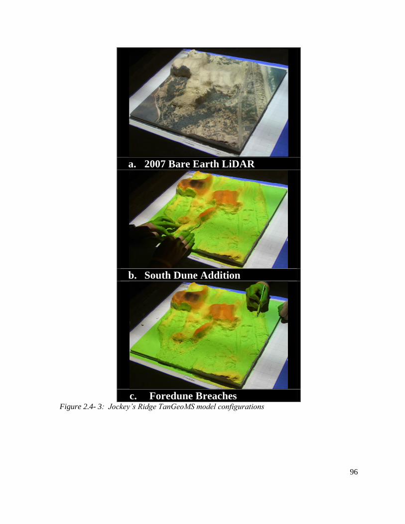
96

a. 2007 Bare Earth LiDAR

b. South Dune Addition

c. Foredune Breaches Figure 2.4- 3: Jockey’s Ridge TanGeoMS model configurations

97

2.4.1 Flooding Simulation with Real World Topography in 2007

An initial model of Jockey’s Ridge was created to simulate coastal flooding based on

the 2007 Bare Earth LiDAR data (figure 2.4-3a). This model was created in order to assess

which areas on the barrier islands would flood due to increased ocean and soundside water

level. Simulations were run on the model by increasing water levels by 0.25m from 0m to

5m relative to NAVD88 (figure 2.4.1-1b). This model was used as a baseline for

comparison with results from model modifications. After coastal flooding simulations were

calculated and projected on the model, ideas for model modifications were formulated.

“TanGeoMS 2007 Bare Earth Flooding” (Weaver K., 2011f) shows the time series of

flooding indicating that low lying areas like Soundside Road flood even at relatively small

increases of water levels. This area commonly floods during intense rain events or storms

(figure 2.4.1-1a). As the water level is increased, flooding continues east along Soundside

Road until it eventually hits Highway 158 with the source of flooding from the Roanoke

Sound. With 1m increase in water level, Soundside Road based off 2007 LiDAR data would

flood halfway between Roanoke Sound and Highway158, while 1.5m rise would have

flooding almost reaching Highway 158 (figure 2.4.1-1b) flooding residential areas south of

the park. Flooding from the soundside is demonstrated because the oceanside foredunes can

withstand water increases up to approximately 4m; dune erosion and degradation is not taken

into account, however.

98

Figure 2.4.1- 1: (a) Images taken after storms along Soundside Road indicting flooding

vulnerability of Soundside Road. (b) 2007 Bare Earth LiDAR model with calculated flooding

projected onto TanGeoMS model demonstrating Soundside Road flooding first at 1m while

the oceanside foredunes retain increases of water level due to their elevations being around

4m.

2.4.2 Impact of South Dune Addition

In 2003 the South Dune (125 x 103

m3 of sand) was removed from the Jockey’s Ridge

dune field, and trucked north of the Main Dune in hopes of feeding the Main Dune (Cox,

Personal communication; Judge et al., 2000; Mitasova et al., 2005). This dune was removed

99

due to it migrating close to homes along Soundside Road. Part of the dune was essentially

touching a home and one way to prevent homes from being claimed by the dune was to

relocate the dune itself (figure 1.1-3a,b). Since removal of the dune, the elevation where the

South Dune used to be is similar to the elevation of the lowest lying areas along Soundside

Road, which flood at the water level of 1m above NAVD88 as shown from the 2007 LiDAR

Bare Earth model simulation (figure 2.4.1-1b).

One question explored using TanGeoMS is what would happen if the South Dune

was allowed to keep migrating south instead of removing it. How would the dune if left to

evolve affect flooding? Would letting this dune continue to migrate protect residential

homes along Soundside Road? This question was tested by simply forming a clay dune on

the physical model that reflected the probable location and landform of the South Dune if it

was allowed to keep migrating south (figure 2.4-3b). After the dune was added to the model

and scanned, the point cloud was imported into GRASS GIS, interpolated and incremental

flooding was calculated for this model at 0.25m increments until 5m water level elevation

(figure 2.4.2-1). “TanGeoMS South Dune Addition” animation shows the impact of water

level rise for this scenario (Weaver K., 2011g). At the 1m mark, a small area along the

soundside floods first while the oceanside dunes withstand the increase due to the 4m

foredunes. The added dune protected the residential areas south of the park up to 1.5m water

level increase compared to the 2007 Bare Earth model where residential areas almost flooded

to Highway 158 (figure 2.4.2-2). The addition of the South Dune or a similar structure

feature indicates that this area may be protected from soundside storm induced flooding by

the addition of a dune or another protective barrier along Soundside Road. However, further

exploration is needed, by allowing the South Dune to keep migrating; homes are in jeopardy

of being claimed by the dune as was the problem in 2003.

100

Figure 2.4.2- 1: Flooding TanGeoMS model after the South Dune was added. Top left

image shows the forming of the dune using clay to the model then flooding was projected on

the model demonstrating how the newly added dune affected coastal flooding. The dune was

able to withstand 1.5m increase of water level protecting residential areas south of Jockey’s

Ridge.

101

Figure 2.4.2- 2: Comparing 2007 Bare Earth model flooding with TanGeoMS South Dune

addition flooding on residential area (red squares). The South Dune addition was able to

withstand a 1.5m water level increase, protecting homes south of Jockey’s Ridge.

2.4.3 Foredune Breaches

Dune breaches created during intense storm activity can also be simulated using

TanGeoMS by simply carving a breach at selected locations along the foredune or soundside

dune. Figure 2.4.3-1a is an example of the progression of a real dune breach during 2003’s

Hurricane Isabel just south of the U.S. Army Corps of Engineers Field Research Facility in

Duck, North Carolina captured from a web camera during the storm (U.S. Army Corps of

Engineers, 2003).

Two areas were selected on the oceanside foredune around the Jockey’s Ridge State

Park. Breaches were carved in the foredune to study the impacts brought about by coastal

flooding and the effects these breaches have on residential flooding dependent upon the

102

breach location and surrounding elevations (Figure 2.4-3c). After the breaches were carved,

the model was scanned then the point cloud was imported into GRASS GIS for referencing,

interpolation and simulations. After simulations were run, the results as an animation,

“TanGeoMS Dune Breaches” or 2D image were projected on the model for rapid feedback

about the areas impacted from the breaches (figure 2.4.3-1b, Weaver K., 2011h). Upon

closer examination and projection of 2009’s digitized homes, flooded areas can be studied to

see which homes are impacted at specific water level increments. At 1.25m rise, water starts

to flood the breaches and at 1.5m rise, homes start flooding while at 1.75m rise low lying

areas start flooding such as roads behind the foredune (figure 2.4.3-2).

103

Figure 2.4.3- 1: (a) Time series of images taken at the U.S. Army Corps of Engineers Field

Research Lab in Duck, North Carolina during Hurricane Isabel showing progression of a

dune breach. (Images courtesy of U.S. Army Corps of Engineers, 2003) (b) TanGeoMS

model demonstrating carving of dune breaches by hand and running flooding simulations

after model modification. Dune breaches begin flooding at the 1.25m level and start flooding

Highway 12 at 1.5m. (Image from Starek et al. 2011)

104

Figure 2.4.3- 2: TanGeoMS dune breach model showing flooding extent due to breaches

(black ovals) around residential homes and businesses (red squares). Residential areas start

flooding at 1.5m water level, at 1.75m water level roads parallel to the foredunes flood due

to breaches.

2.5 Discussion

Our exploratory system incorporates a 3D tangible user interface with GIS

capabilities. TanGeoMS is a promising interactive geospatial tool for modifying, visualizing

and analyzing terrain. The system provides opportunities for people to collaborate and create

physical topographical models that can be used in the research and education as well as in

classrooms and museums for decision-making and educational opportunities. The system

provides insight into how modifications to terrain make an impact on desired parameters

such as flooding, erosion, runoff, etc. The results of TanGeoMS analysis and simulations

projected over the clay models allow users to explore a large number of diverse terrain

configurations in a collaborative setting.

The application of the TanGeoMS system has been demonstrated on many diverse

environments, however, this chapter focuses on the coastal application of TanGeoMS and the

future possibilities, capabilities and benefits of using this system to analyze and investigate

dynamic coastal landscapes.

105

The benefit from this system is that it not only incorporates point and click GIS

capabilities, but it provides a tangible user interface that allows for collaboration and the

physical use of hands to create landscape modifications that help define the most important

scenarios that need to be accurately modeled to asses potential impacts.

TanGeoMS is in the preliminary development stage that still requires significant

improvements and modifications before it can be routinely used for research and education.

Future work on the system is to foster a faster, fully automated model to GIS to model

processing by creating an interface within GRASS GIS that is specifically tailored to

TanGeoMS. This interface would interpolate the scanned data, run analysis then project the

results back onto the model providing near real-time results.

Currently, models are being constructed by hand and errors from the user can be

introduced to the model due to carving techniques. Allowing the models to get

professionally carved using a 3D printer will create more accurate and durable models.

Mobile TanGeoMS is in the preliminary stage as well, a more mobile and lighter

stand is currently being designed in order to create an easier and mobile system for

demonstration purposes at conferences, workshops, meetings, schools, etc (figure 2.5-1b).

Currently half of TanGeoMS is part of the mobile system, since the scanner is located in

VISSTA labs on North Carolina State University’s campus, only pre-calculated model results

can be projected onto the model since the scanner is too large to travel. A hand held scanner

has been developed that we hope to incorporate into the mobile system in order to complete

the mobile TanGeoMS.

106

Figure 2.5- 1: Helena Mitasova and Katherine Weaver demonstrating TanGeoMS to North

Carolina State University’s Chancellor Woodson using the mobile system.

2.6 Conclusions

The capabilities of TanGeoMS are demonstrated by studying areas that are

vulnerable to coastal flooding due to failures in foredunes during storms as well as simulate

the effects of extending dunes to simulate dune migration. These are simulated by carving

foredune breaches and creating a dune that mimics the South Dune as if it was left to migrate

south since 2003’s removal. Flooding was simulated using the simplistic “bathtub” model

where water levels are increased at specific increments relative to NAVD88 in order to study

the extent of flooding around coastal areas.

This research demonstrates the capability of using TanGeoMS in coastal areas;

these results, however, do not reflect actual real world-tested results due to the system

remaining in the preliminary stage. This research is intended to propose the benefit of using

a tangible system such as TanGeoMS in the future to further study coastal terrain.

Results and user feedback from these simulations and past model simulations indicate

that TanGeoMS is a promising tool for 3D tangible terrain exploration and after future

107

system modifications and improvements will benefit terrain research by allowing

collaboration in a setting that requires relatively no knowledge of GIS. Although the system

still has limitations, the applications we present illustrate its potential for improving our

understanding of interactions between landforms and landscape processes and

communicating these interactions to audiences with diverse backgrounds.

2.7 References

Brown, E., Overton, M., 2011. Visualizing evolving landforms due to sea level rise,

Coastal Sediments ’11, Miami, Florida.

Cox, Jennifer, 26 January, 2011. Jockey’s Ridge Ranger. Personal communication by phone.

Cruz-Neira, C., Sandin, D. J., DeFanti, T. A., Kenyon, R. V., Hart, J. C., 1992. The CAVE:

audio visual experience automatic virtual environment. Communications of the ACM,

35(6), 64–72.

Defense Update, 2005a. The Modern Command Post Tactical Operations Center, Defense

Update, International Online Defense Magazine, 3, 8.

http://defense-update.com/features/du-3-05/c4i-8.htm (accessed 13 June, 2011).

Defense Update, 2005b. TouchTable Collaboration & Presentation Display, Defense Update,

International Online Defense Magazine 3.

http://defense-update.com/products/t/touchtable.htm (accessed 13 June, 2011).

Johnson, A., Leigh, J., Morin, P., Van Keken, P., 2006. GeoWall: stereoscopic visualization

for geoscience research and education. IEEE Computer Graphics and Applications,

26 (6), 10–14.

Judge, E.K., Courtney, M.G., Overton, M.F., 2000. Topographic Analysis of Dune Volume

and Position, Jockey’s Ridge State Park, North Carolina. Shore and Beach, 68(4), 19–

24.

Mitasova, H., Mitas, L., Ratti, C., Ishii, H., Alonso, J., Harmon, R.S., 2006. Real-time human

interaction with landscape models using a tangible geospatial modeling environment.

IEEE Computer Graphics & Applications, Special Issue-GeoVisualization ,26(4), 55–

63.

http://defense-update.com/features/du-3-05/c4i-8.htm

http://defense-update.com/products/t/touchtable.htm

108

Mitasova, H., Overton, M., Harmon, R.S., 2005. Geospatial analysis of a coastal sand dune

field evolution: Jockey’s Ridge, North Carolina. Geomorphology, 72, 204-221.

Mitasova H., Harmon R.S,. Weaver K., Lyons, N., Overton, M., 2011. Scientific

visualization of landscapes and landforms, Geomorphology, In Press, Corrected

Proof, Available online 13 June 2011.

Neteler, M., Mitasova, H., 2008. Open Source GIS: A GRASS GIS Approach, Third edition.

Springer, NY.

North Carolina Floodplain Mapping Program., 2011. Floodplain Mapping Information

System (FMIS). http://floodmaps.nc.gov/fmis/ (accessed 29 July, 2011).

Piper, B., Ratti, C., Ishii, H., 2002. Illuminating Clay: A Tangible Interface with potential

GRASS applications, Proceedings of the Open Source GIS-GRASS users conference,

Trento, Italy, 11-13 September 2002.

Starek, M.J., Mitasova, H., Hardin, E., Weaver, K., Overton, M., Harmon, R.S., 2011,

Modeling and Analysis of Landscape Evolution at Multiple Scales Using Airborne,

Terrestrial, and Laboratory Laser Scanning, Geosphere (accepted).

Tateosian, L. G., Mitasova, H., Harmon, B. A., Fogleman, B., Weaver, K.,Harmon, R.S.,

2010. TanGeoMS: A Tangible geospatial modeling system. IEEE Transactions on

Visualization and Computer Graphics (Proceedings InfoVis 2010). 16(6), 1605-1612.

Underkoffler, J., Ishii, H., 1999. Urp: a luminous-tangible workbench for urban planning and

design. Proceedings of the Conference on Human Factors in Computing Systems

(CHI '99), 15–20 May 1999, Pittsburgh, PA, USA. 386–393.

U.S. Army Corps of Engineers., 2003. Hurricane Isabel Video Stills.

http://www.frf.usace.army.mil/isabel/video/page_01.html (accessed 26 July, 2011)

Weaver, K, 2011f, TanGeoMS 2007 Bare Earth Flooding,


Weaver, K, 2011g, TanGeoMS South Dune Addition,


Weaver, K, 2011h, TanGeoMS Dune Breaches,


http://floodmaps.nc.gov/fmis/

http://www.frf.usace.army.mil/isabel/video/page_01.html



109

APPENDIX

110

Appendix A. Baseline Data Scripts

111

Appendix B. Dune Peak Extraction Scripts

Code used in GRASS GIS to extract dune peaks for each dune of Jockey’s ridge:

d.rast -o map=JR_YEAR@Baseline_JR vallist=vallist (RANGE)

*A Jockey’s Ridge DEM from the time series will be the input for JR_Year found under the YEAR column

below. The input for Vallist (RANGE) are the elevations under the Vallist (RANGE) column for each DEM.

Dune Peak YEAR Vallist (RANGE: elevations in meters)

Main

1974 33.53

1995 26.04

1998 23.9-30

1999 26.43

2001 25.06

2007 20.81

2008 21.56

West 1

1995 20.134-30

1998 19.55-25

1999 21.175-30

2001 21.29-30

2007 21.54-30

2008 22.35-30

West 2

1974 20.61-30

1995 20.18-30

1998 20.19-30

1999 20.37-30

2001 20.46-30

2007 20.7-30

2008 20.94-30

East 1

1974 20.218-30

1995 16.809-30

1998 16.52-30

1999 17.7-30

2001 17.92-30

2007 18.32-30

2008 19.59-30

East 2

1974 20.218-30

1995 16.8-30

1998 15.44-30

1999 16.19-30

2001 15.305-30

2007 14.84-30

2008 15.21-30

112

Appendix C. Sand Volume Calculation Scripts

Appendix D. Dune Slip Face Extraction Scripts

Appendix E. Dune Crest Extraction Scripts

113

Appendix F. Imagery Classification Script # ****************************************************************************************

# Name: Image_Classification.py

# Created by: Katherine Weaver (4-6-2011)

# Purpose: Imports raster images (tiffs) and classifies each image into vegetation, sand and development (Uses

# images from 1932 to 2009). ***Works on Windows machines***

# ****************************************************************************************

# Import the modules to make python work with GRASS

import os

# This is the path where the image (tiff files) to be classified are located.

mydir = "C:\\Temp\\Thesis_Images"

mapset="@Thesis_Imagery"

# Walk through directories and pull out tif files

Image_Path_list=[]

for (path, dirs, files) in os.walk(mydir):

for i in files:

JR_tif=str(i)

if( JR_tif.endswith('tif')):

Image_Path_list.append(path+"\\"+JR_tif)

#print Image_Path_list

# Setting the initial region to bounds of vegetation extraction area

os.system("g.region n=251950.83449587 s=249336.1548403 e=914125.59235817 w=911938.02372514 res=1")

os.system("g.region -p")

for image in Image_Path_list:

# Importing images into GRASS GIS

command_Importing="r.in.gdal -o --overwrite input="+image+"

output="+"JRs_"+os.path.basename(image)[:-4]

#print command_Importing

os.system(command_Importing)

# Masking out area needed for extraction for bands .1, .2 and .3

command_mask_Band1="r.mapcalc JR_"+os.path.basename(image)[:-

4]+".1="+"JRs_"+os.path.basename(image)[:-4]+".1*Image_mask"

os.system(command_mask_Band1)

#print command_mask_Band1




#print command_Resolution_Band2




#print command_mask_Band3

114

# Setting the region to each image in order to classify

command_Image_Region="g.region rast=JR_"+os.path.basename(image)[:-4]+".1"+mapset+" res=1"

#print command_Image_Region

os.system(command_Image_Region)

os.system("g.region -p")

# Changing image resolution to 1 meter for bands .1, .2 and .3

command_Resolution_Band1="r.mapcalc JR_"+os.path.basename(image)[:-

4]+"_1m.1="+"JR_"+os.path.basename(image)[:-4]+".1"

os.system(command_Resolution_Band1)










#Deleting initial bands (different resolutions)

#command_delete="g.remove rast=JR_"+os.path.basename(image)[:-

4]+".1,JR_"+os.path.basename(image)[:-4]+".2,JR_"+os.path.basename(image)[:-4]+".3"

#print command_delete

#os.system(command_delete)

# Grouping

command_Grouping="i.group group="+"JR_"+os.path.basename(image)[:-4]+"

subgroup="+"JR_"+os.path.basename(image)[:-4]+" input=JR_"+os.path.basename(image)[:-

4]+"_1m.1,JR_"+os.path.basename(image)[:-4]+"_1m.2,JR_"+os.path.basename(image)[:-4]+"_1m.3"

os.system(command_Grouping)

#print command_Grouping

# Clustering

command_Clustering="i.cluster group=JR_"+os.path.basename(image)[:-4]+"

sub=JR_"+os.path.basename(image)[:-4]+" sig=sig_JR_"+os.path.basename(image)[:-4]+" classes=10

report=report_JR_"+os.path.basename(image)[:-4]+".txt"

#print command_Clustering

os.system(command_Clustering)

# Maximum Likelyhood Classification

command_Maxlik="i.maxlik --overwrite group=JR_"+os.path.basename(image)[:-4]+"

sub=JR_"+os.path.basename(image)[:-4]+" sig=sig_JR_"+os.path.basename(image)[:-4]+"

class=JR_"+os.path.basename(image)[:-4]+"_maxlik10 rej=JR_"+os.path.basename(image)[:-

4]+"_maxlik10_rej"

#print command_Maxlik

os.system(command_Maxlik)

115

Appendix G. TanGeoMS Example Model Script

116

Appendix H. Horizontal Dune Crest Migration Table

Year West Dune South Face Rate of Change

(m/yr) Main Dune South Face

Rate of Change (m/yr)

1974 0.00 0.00

1995 52.96 2.52 85.35 4.06

1998 62.71 3.25 95.75 3.46

1999 71.91 9.20 105.20 9.45

2001 84.08 6.08 92.00 -6.60

2007 121.67 6.27 106.60 2.43

2008 121.70 0.03 121.00 14.40

Year Main Dune Finger Face Rate of change

(m/yr) Main East

Face Rate of change

(m/yr)

1974 0.00 0.00

1995 34.67 1.65 36.75 1.75

1998 50.74 5.36 38.60 0.62

1999 62.31 11.57 62.41 23.81

2001 68.51 3.10 90.91 14.25

2007 108.20 6.62 98.32 1.23

2008 110.90 2.70 102.71 4.39

Year East Dune South Face

Rate of Change

(m/yr)

1974 0.00

1995 88.70 4.22

1998 113.63 8.31

1999 128.37 14.73

2001 139.43 5.53

2007 167.03 4.60

2008 178.73 11.70

117

Appendix I. Horizontal Dune Peak Migration Tables

Year West Dune 2 Rate of Change

(m/yr) West Dune 1 Rate of Change

(m/yr)

1974 0.00 0.00 0.00 0.00

1995 80.47 3.83 35.28 1.68

1998 151.74 6.32 62.34 2.60

1999 183.33 7.33 111.89 4.48

2001 236.06 8.74 126.94 4.70

2007 267.92 8.12 196.19 5.95

2008 294.35 8.66 233.17 6.86

Year Main Dune Rate of Change

(m/yr) East Dune 1 Rate of Change

(m/yr)

1974 0.00 0.00 0.00 0.00

1995 54.37 2.59 53.61 2.55

1998 63.78 2.66 98.19 4.09

1999 83.25 3.33 126.32 5.05

2001 111.99 4.15 154.51 5.72

2007 128.26 3.89 212.39 6.44

2008 143.27 4.21 217.45 6.40

Year East Dune 2

Rate of Change

(m/yr)

1974 0.00 0.00

1995 97.33 4.63

1998 132.48 5.52

1999 185.81 7.43

2001 222.22 8.23

2007 275.04 8.33

2008 296.33 8.72

118

Appendix J. Imagery Available for Jockey’s Ridge

Orthophotos

Year Imagery

1993 Black and White

1996 Black and White

1998 Color Infrared (CIR)

2006 Color

2007 Color

2008 Color (IR?)

2009 Infrared

2010 Color (IR pending)

Documents

Jockey’s Ridge State Park, loca ’s