Jianlin  Cheng,  PhD  Computer  Science  Department  University  of  Missouri,  Columbia  

Fall,  2013    

•  Princeton’s  class  notes  on  linear  programming  •  MIT’s  class  notes  on  linear  programming  •  Xian  Jiaotong  University’s  class  notes  on  linear  programming  

•  Ohio  University’s  class  notes  •  Rutgers  University’s  class  notes  

•  Essen>al  tool  for  op>mal  alloca>on  of  scarce  resource  among  a  number  of  compe>ng  ac>vi>es  

•  Powerful  and  general  problem-­‐solving  method        -­‐  shortest  path,  max  flow,  min  cost  flow            minimum  spanning  tree  

•  Fast  commercial  solvers:  CPLEX,  OSL  •  Ranked  among  most  important  scien>fic  advances  of  20th  century  

•  Also  a  general  tool  for  aQacking  NP-­‐hard  op>miza>on  problems  

•  Dominates  world  of  industry        -­‐  ex:  Delta  claims  saving  $100  million  per  year              using  LP  

•  Agriculture:  diet  problem  •  Computer  science:  data  mining  •  Electrical  engineering:  VLSI  design  •  Energy:  blending  petroleum  products  •  Environment:  water  quality  management  •  Finance:  porYolio  op>miza>on  •  Logis>cs:  supply-­‐chain  management  •  Management:  hotel  yield  management  •  Marke>ng:  direct  mail  adver>sing  •  manufacturing:  produc>on  line  balancing  •  Medicine:  radioac>ve  seed  placement  in  cancer  treatment  •  Opera>on  research:  airline  crew  assignment  •  Telecommunica>on:  network  design,  internet  rou>ng  •  Sports:  scheduling  ACC  basketball  

An  Example,  IntuiFve  Understanding  of  Linear  Programming  

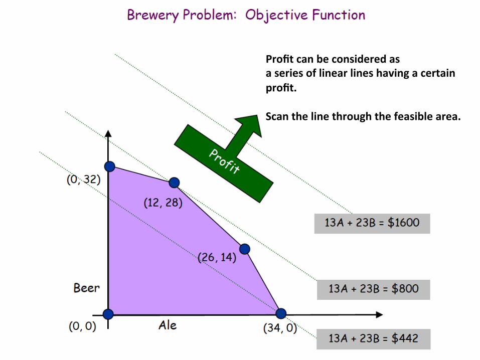
Profit  can  be  considered  as    a  series  of  linear  lines  having  a  certain  profit.    Scan  the  line  through  the  feasible  area.  

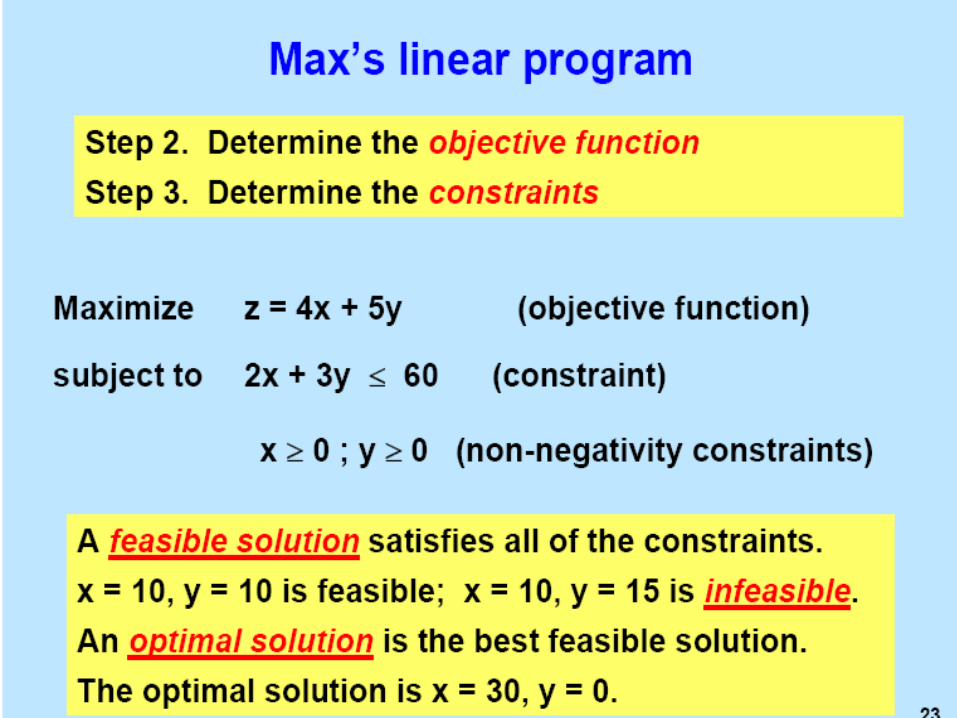
Another  Example,  FormulaFon,  and  Proof  

.0,9,0 6032 s.t.54 min

≥≥≥

=++

−−=

wyxwyx

yxzax

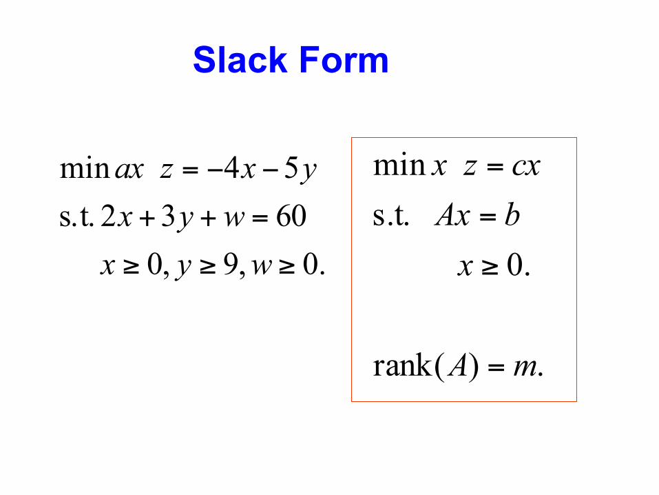
Slack Form

.)(rank

.0 s.t.

min

mA

xbAxcxzx

=

≥

=

=

6032 ≤+ yx

yxz 54 +=

Feasible domain

Optimal occurs at a vertex!!!

What’s a vertex?

. ,),(21

if vertexa called is polyhadren ain point A

zyxzyzyx

x

==Ω∈+=

Ω

⇒

. of sin vertice found becan it then solution, optimalan has over min If

.}0|{Let

Ω

Ω∈

≥Ω

xcx Ax = b, xx =

Fundamental Theorem

.constraint oneleast at violates' is, that ,in not 'point a havemust line theThus, line.any contain not

does However, solutions. optimal are *)( lineon points feasible all that followsIt solutions. optimal

also are and that means This . havemust we2,)( and ,

,* Since distinct. are ,*, and 2/)(*such that ,exist thereis, that not, is * suppose

on,contraditiBy . of vertex a is * that show willWesolutions. optimal all among components zero of

number maximum with *solution optimalan Consider

xx

y-xx*+

zy czcx* = cy =/cy+czcx* = czcx*

cycxzyxzyxzyx

x

x

Ω

Ω

≤

≤+=

Ω∈

Ω

α

Proof.

infinite  

X*  

Y  

Z  

X’  

X’  violates  one  constraint  

ion.contradict a,*than component -zero more one has which ,* and'between solution optimalan findeasily can weNow,

.0 with somefor 0 constraint a violatemust ' Hence, 0. constraint latecannot vio '

that means This .any for 0 toequal is *)( ofcomponent th theTherefore, .0* havemust

we,0 and 2/)( since ,0for Moreover, . constraint latecannot vio ' Thus,

.*))(( ,any for that Note

xxx

*>xjxxxx

y-xx*+i==x=yz

,zy+zy*=x* =xAx = bx

= by-xx*+A

jj

i

iii

iiiiii

≥

≥

≥

αα

αα

Proof (cont’s).

X*  

Y  

Z  

X’  

X’  has  fewer  or  equal  number  of    0  terms  as  X*.  X’  has  one  nega>ve  component,  whose  value  in  X*  is  posi>ve.  As  we  move  from  X’  to  X*  into  the  feasible  region,  the  component  will  become  0    

Polyhedron  of  simplex  algorithm  in  3D  

Demo  of  MIT  Linear  Programming  Solver:    

hQp://sourceforge.net/projects/lipside/  

Integer Programming •  Integer programming is a solution method for many

discrete optimization problems •  Programming = Planning in this context •  Origins go back to military logistics in WWII (1940s). •  In a survey of Fortune 500 firms, 85% of those

responding said that they had used linear or integer programming.

•  Why is it so popular? –  Many different real-life situations can be modeled as integer

programs (IPs). –  There are efficient algorithms to solve IPs.

Standard form of integer program (IP)

maximize c1x1+c2x2+…+cnxn (objective function) subject to

a11x1+a12x2+…+a1nxn ≤ b1 (functional constraints) a21x1+a22x2+…+a2nxn ≤ b2 …. am1x1+am2x2+…+amnxn ≤ bm x1, x2 , …, xn ∈ Z+ (set constraints)

Standard form of integer program (IP) •  In vector form:

maximize cx (objective function) subject to Ax ≤ b (functional constraints) x ∈ (set constraints)

Input for IP: 1×n vector c, m×n matrice A, m×1 vector b. Output of IP: n×1 integer vector x . •  Note: More often, we will consider

mixed integer programs (MIP), that is, some variables are integer,

the others are continuous.

n+Z

Example of Integer Program (Production Planning-Furniture Manufacturer)

•  Technological data: Production of 1 table requires 5 ft pine, 2 ft oak, 3 hrs labor 1 chair requires 1 ft pine, 3 ft oak, 2 hrs labor 1 desk requires 9 ft pine, 4 ft oak, 5 hrs labor

•  Capacities for 1 week: 1500 ft pine, 1000 ft oak, 20 employees (each works 40 hrs).

•  Market data:

•  Goal: Find a production schedule for 1 week

that will maximize the profit.

profit demand table $12/unit 40 chair $5/unit 130 desk $15/unit 30

Production Planning-Furniture Manufacturer: modeling the problem as integer program

The goal can be achieved by making appropriate decisions.

First define decision variables: Let xt be the number of tables to be produced;

xc be the number of chairs to be produced; xd be the number of desks to be produced. (Always define decision variables properly!)

Production Planning-Furniture Manufacturer: modeling the problem as integer program

Ø Objective is to maximize profit: max 12xt + 5xc + 15xd

Ø  Functional Constraints capacity constraints: pine: 5xt + 1xc + 9xd ≤ 1500

oak: 2xt + 3xc + 4xd ≤ 1000 labor: 3xt + 2xc + 5xd ≤ 800 market demand constraints: tables: xt ≥ 40 chairs: xc ≥ 130 desks: xd ≥ 30

Ø Set Constraints xt , xc , xd ∈ Z+

Solutions to integer programs •  A solution is an assignment of values to variables. •  A feasible solution is an assignment of values to

variables such that all the constraints are satisfied. •  The objective function value of a solution is obtained

by evaluating the objective function at the given point. •  An optimal solution (assuming maximization) is one

whose objective function value is greater than or equal to that of all other feasible solutions.

•  Integer program is NP complete •  There are efficient algorithms for finding the optimal

solutions of an integer program based on LP relaxation.

Next: IP modeling techniques Modeling techniques:

Ø Using binary variables Ø Restrictions on number of options Ø Contingent decisions Ø Variables with k possible values

Applications: Ø Facility Location Problem Ø Knapsack Problem

Example of IP: Facility Location •  A company is thinking about building new facilities in

LA and SF. •  Relevant data:

Total capital available for investment: $10M •  Question: Which facilities should be built

to maximize the total profit?

capital needed expected profit 1. factory in LA $6M $9M 2. factory in SF $3M $5M

3. warehouse in LA $5M $6M 4. warehouse in SF $2M $4M

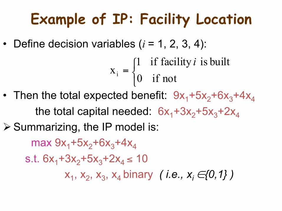
Example of IP: Facility Location •  Define decision variables (i = 1, 2, 3, 4):

•  Then the total expected benefit: 9x1+5x2+6x3+4x4 the total capital needed: 6x1+3x2+5x3+2x4

Ø Summarizing, the IP model is: max 9x1+5x2+6x3+4x4

s.t. 6x1+3x2+5x3+2x4 ≤ 10 x1, x2, x3, x4 binary ( i.e., xi ∈{0,1} )

⎩⎨⎧

=not if 0

built is facility if 1x i

i

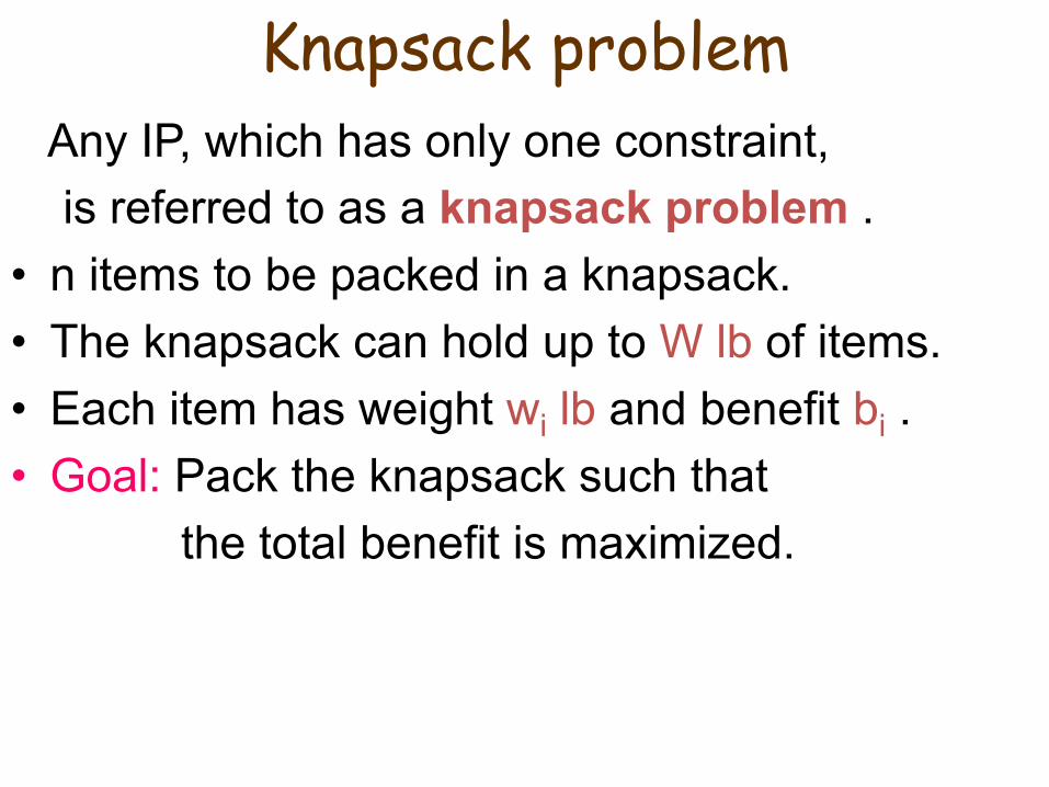
Knapsack problem Any IP, which has only one constraint, is referred to as a knapsack problem .

•  n items to be packed in a knapsack. •  The knapsack can hold up to W lb of items. •  Each item has weight wi lb and benefit bi . •  Goal: Pack the knapsack such that

the total benefit is maximized.

IP model for Knapsack problem •  Define decision variables (i = 1, …, n):

•  Then the total benefit: the total weight:

Ø Summarizing, the IP model is: max s.t. xi binary (i = 1, …, n)

⎩⎨⎧

=not if 0

packed is item if 1x i

i

∑=

n

iii xb

1 ∑=

n

iii xw

1

∑=

n

iii xb

1

Wxwn

iii ≤∑

=1

Connection between the problems •  Note: The version of the facility location

problem is a special case of the knapsack problem.

Ø Important modeling skill: – Suppose you know how to model Problem A1,…,Ap; – You need to solve Problem B; – Notice the similarities between Problems Ai and B; – Build a model for Problem B, using the model for

Problem Ai as a prototype.

The Facility Location Problem: adding new requirements

•  Extra requirement: build at most one of the two warehouses. The corresponding constraint is: x3 +x4 ≤ 1

•  Extra requirement: build at least one of the two factories. The corresponding constraint is: x1 +x2 ≥ 1

Modeling Technique: Restrictions on the number of options

•  Restrictions: At least p and at most q of the options can be chosen.

•  The corresponding constraints are:

pxn

ii ≥∑

=1qx

n

ii ≤∑

=1

Modeling Technique: Contingent Decisions Back to the facility location problem. •  Requirement: Can’t build a warehouse unless

there is a factory in the city. The corresponding constraints are: x3 ≤ x1 (LA) x4 ≤ x2 (SF)

•  Requirement: Can’t select option 3 unless at least one of options 1 and 2 is selected. The constraint: x3 ≤ x1 + x2

•  Requirement: Can’t select option 4 unless at least two of options 1, 2 and 3 are selected. The constraint: 2x4 ≤ x1 + x2 + x3

Modeling Technique: Variables with k possible values

•  Suppose variable y should take one of the values d1, d2, …, dk .

•  How to achieve that in the model? •  Introduce new decision variables. For i=1,…,k,

•  Then we need the following constraints.

⎩⎨⎧

=otherwise 0

d valuey takes if 1x i

i

value)oneonly can take ( 11

yxk

ii =∑

=

1) xif d value takeshould ( ii1

==∑=

yxdyk

iii

■  Rounding  non-­‐integer  solu/on  values  up  to  the  nearest  integer  value  can  result  in  an  infeasible  solu/on.  

■  A  feasible  solu/on  is  ensured  by  rounding  down  non-­‐integer  solu>on  values  but  may  result  in  a  less  than  op>mal  (sub-­‐op/mal)  solu/on.  

Integer  Programming  Example  Graphical  SoluFon  of  Machine  Shop  Model  

Maximize Z = $100x1 + $150x2 subject to: 8,000x1 + 4,000x2 ≤ $40,000 15x1 + 30x2 ≤ 200 ft2

x1, x2 ≥ 0 and integer Optimal Solution:

Z = $1,055.56 x1 = 2.22 presses x2 = 5.55 lathes

Figure 5.1 Feasible Solution Space with Integer Solution Points Copyright © 2010 Pearson Education, Inc. Publishing as Prentice Hall

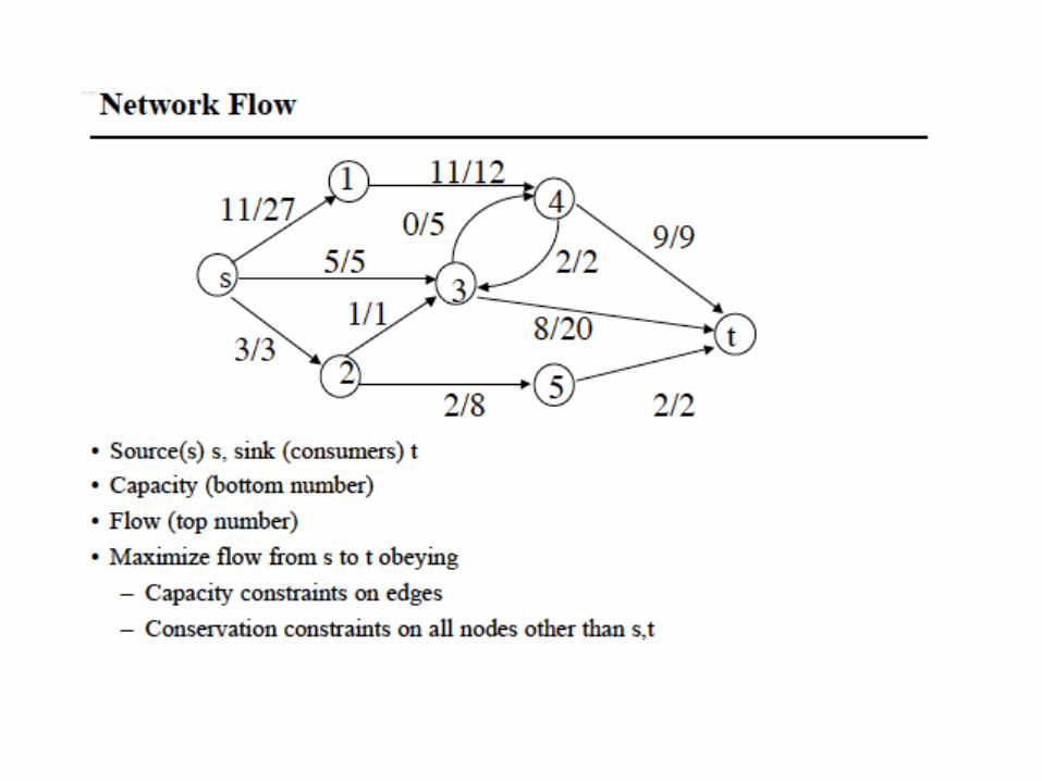
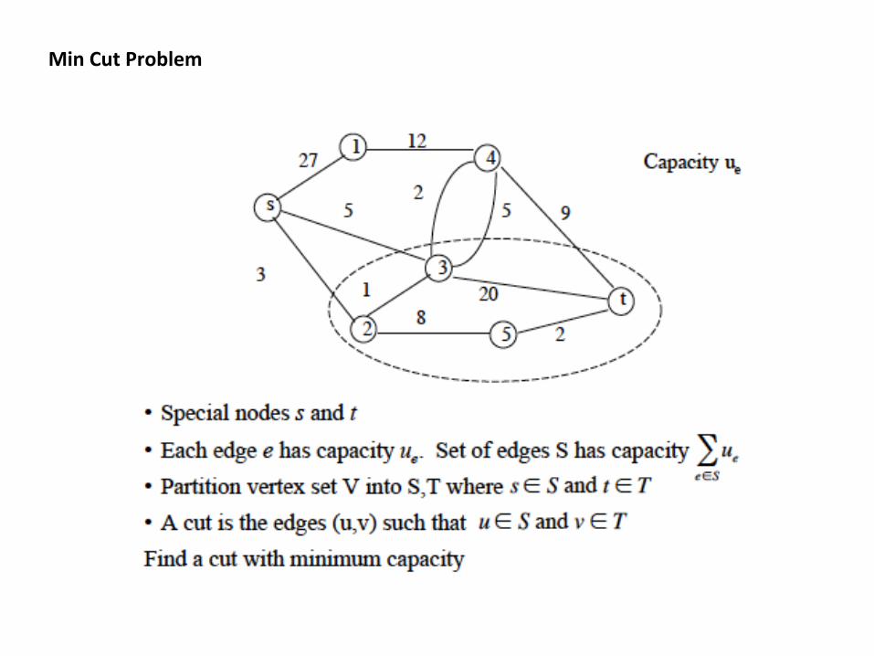
Min  Cut  Problem  

Algorithms  

•  Use  IP  to  solve  the  network  flow  problem  •  Use  IP  to  solve  the  min-­‐cut  problem