arX

iv:a

stro

-ph/

0508

426v

1 1

9 A

ug 2

005

to be published in the MNRAS (2005)

Jets, Structured Outflows, and Energy Injection in GRB

Afterglows: Numerical Modelling

A. Panaitescu2511 Speedway, Department of Astronomy, University of Texas at Austin, Austin, TX 78712

Space Science and Applications, MS D466, Los Alamos National Laboratory, Los Alamos, NM 87545

ABSTRACTWe investigate numerically the ability of three models (jet, structured outflow, energy injection) to

accommodate the optical light-curve breaks observed in 10 GRB afterglows (980519, 990123, 990510,

991216, 000301c, 000926, 010222, 011211, 020813, and 030226), as well as the relative intensities

of the radio, optical, and X-ray emissions of these afterglows. We find that the jet and structured

outflow models fare much better than energy injection model in accommodating the multiwavelength

data of the above 10 afterglows. For the first two models, a uniform circumburst medium provides a

better fit to the optical light-curve break than a wind-like medium with a r−2 stratification. However,

in the only two cases where the energy injection model may be at work, a wind medium is favoured

(an energy injection is also possible in a third case, the afterglow 970508, whose optical emission

exhibited a sharp rise but not a steepening decay). The best fit parameters obtained with the jet

model indicate an outflow energy of 2−6×1050 ergs and a jet opening of 2o−3o. Structured outflows

with a quasi-uniform core have a core angular size of 0.7o − 1.0o and an energy per solid angle of

0.5 − 3 × 1053 ergs sr−1, surrounded by an envelope where this energy falls-off roughly as θ−2 with

angle from the outflow axis, requiring thus the same energy budget as jets. Circumburst densities

are found to be typically in the range 0.1 − 1 cm−3, for either model. We also find that the reverse

shock emission resulting from the injection of ejecta into the decelerating blast wave at about 1 day

after the burst can explain the slowly decaying radio light-curves observed for the afterglows 990123,

991216, and 010222.

Key words: gamma-rays: bursts - ISM: jets and outflows - radiation mechanisms:non-thermal - shock waves

1 INTRODUCTION

Since the prediction of radio (Paczynski & Rhoads 1993) andoptical transients (Meszaros & Rees 1997) associated withGRBs, more than 100 afterglows have been observed (in-cluding X-ray transients). Good monitoring in all three fre-quency domains has been achieved for about 20 afterglows;the radio, optical, and X-ray flux was observed to decay as apower-law, Fν ∝ t−α (α > 0), confirming the expectations.For 10 of these well-observed afterglows – 980519, 990123,990510, 991216, 000301c, 000926, 010222, 012111, 020813,030226 – the optical light-curve decay exhibits a steepeningat about 1 day after the burst, with an increase ∆α in thetemporal index as low as 0.4 (afterglow 991216) and as highas 1.8 (afterglow 000301c). Optical light-curve breaks haveor may have been observed in other afterglows; they are notincluded in the sample of afterglows modelled in this workbecause those afterglows have been adequately monitored atonly one optical frequency.

With the exception of the afterglow 010222, for whichone, late (10 days) measurement suggests that a break oc-curred also in the X-ray light-curve, currently available X-

ray observations do not extend sufficiently before and afterthe optical break time to prove that the light-curve break isachromatic. Within the measurement uncertainties, a singlepower-law fits well the decay of all adequately monitored X-ray afterglows: 990123, 990510, 991216, 000926 (and 010222until the last measurement).

Breaks, in the form of peaks, have been observed in theradio emission of all 10 afterglows above, usually at ∼ 10days after the burst, i.e. often occurring after the opticallight-curve break. Given that the radio and optical breaksare not simultaneous, they cannot both arise from the dy-namics of the afterglow, the structure of the GRB ejecta, orsome property of the circumburst medium (CBM), as thesemechanisms should yield achromatic breaks. Furthermore,given that, before their respective breaks, the radio emis-sion rises while the optical falls-off, these temporal featurescannot be due to the passage of the same afterglow contin-uum break through the observing band.

With the possible exception of the afterglow 990123,there is no evidence for an evolution (softening) of the op-tical continuum across the light-curve break for the above10 afterglows (e.g. Panaitescu 2005). Furthermore, the only

c© 2005 RAS

2 A. Panaitescu

spectral feature whose passage could yield the large steep-ening ∆α observed in some cases – the peak of the forwardshock (FS) continuum⋆– should yields a rising or flat opticallight-curve before the break, contrary to what is observed.Therefore, it is the radio peak which should be attributed toa spectral break crossing the observing domain. That spec-tral break should be the injection frequency νi, which, forreasonable shock microphysical parameters, should reach theradio at around 10 days. Indeed, for the afterglow 991208,there is observational evidence (Galama et al. 2000) thatthe peak of the afterglow continuum crosses the 10–100 GHzdomain at that time. Further evidence for the passage of aspectral break through radio is provided by that the peaktime of the radio flux of the afterglow 030329 increases withdecreasing observing frequency (Frail et al. 2005).

Today, the generally accepted reason for the opticallight-curve break is the narrow collimation of the GRBejecta. As predicted by Rhoads (1999), if the GRB ejectaare collimated, then the afterglow light-curve should exhibita steepening when the jet begins to expand sideways. Morethan half of the steepening ∆α is due by the finite angu-lar opening of the jet: as the GRB remnant is decelerated(by sweeping-up of the CBM) and the relativistic Dopplerbeaming of the afterglow emission decreases, an ever increas-ing fraction of the emitting surface becomes visible to theobserver; when the jet edge is seen, that fraction cannotincrease any longer and the afterglow emission exhibits afaster decay (Panaitescu, Meszaros & Rees 1998). Becauseit arises from the blast wave dynamics, a light-curve breakshould also be present at radio wavelengths at the same timeas the optical break. However, radio observations before 1day are very scarce and strongly affected by Galactic inter-stellar scintillation (Goodman 1997) until after 10 days, thusthey cannot disentangle the jet-break from that arising fromthe passage of the FS peak frequency.

Another mechanism for the optical light-curve breakshas been proposed by Rossi, Lazzati & Rees (2002) andZhang & Meszaros (2002): if GRB outflows are endowedwith an angular structure (i.e. non-uniform distribution ofthe ejecta kinetic energy with direction), as first proposedby Meszaros, Rees & Wijers (1998), then a steepening of theafterglow decay would arise when the brighter, outflow sym-metry axis becomes visible to the observer. In this model,the stronger the angular structure is, the larger the breakmagnitude ∆α should be.

A third mechanism for breaks rests on the proposal ofPaczynski (1998) and Rees & Meszaros (1998) that the FSenergizing the CBM could be refreshed by the injection of asubstantial energy through some delayed ejecta which werereleased at the same time with the GRB-producing ejecta,but had a smaller Lorentz factor, or were ejected sometimelater, and which catch up with the decelerating FS duringthe afterglow phase. Fox et al. (2003) have proposed that theearly (0.003–0.1 day), slow decay of the optical emission ofthe afterglow 021004 is caused by such an injection process.In this scenario, when the energy injection episode ends, the

⋆ This is the smallest of the synchrotron frequency νi correspond-ing to the typical post-shock electron energy (which we call ”in-jection frequency”) and to the electrons which cool radiatively ona dynamical timescale (the cooling frequency νc)

FS deceleration becomes faster and the afterglow emissionshould exhibit a steepening.

Note the various origins of the afterglow light-curvebreak in each model. In the Jet model, the break is causedby the changing outflow dynamics when the jet starts tospread and by the outflow’s geometry. In the StructuredOutflow (SO) model the origin is, evidently, the outflow’sanisotropic surface brightness. For both these models, spe-cial relativity effects play an important part. In the EnergyInjection (EI) model, the break originates in the alteredoutflow dynamics at the time when the energy injection sub-sides.

The purpose of this work is to compare the ability ofthese three models in accommodatingi) the shape of the light-curve breaks observed in the opticalemission of the afterglows 980519, 990123, 990510, 991216,000301c, 000926, 010222, 012111, 020813, 030226 andii) the relative intensity of the radio, optical, and X-rayemissions of these afterglows,for either a uniform (i.e. homogeneous) CBM, or one witha r−2 density radial stratification, as expected if GRBs pro-genitors are massive stars (Woosley 1993, Paczynski 1998).

For the first task above, we performed an analyticaltest of the models (see table 2 of Panaitescu 2005), basedon comparingi) the pre- and post-break optical light-curve decay indices,α1 and α2,ii) those in the X-rays,iii) the slopes βo and βx of the power-law optical and X-raycontinua (Fo ∝ ν−βo and Fx ∝ ν−βx), andiv) the optical–to–X-ray spectral energy distribution (SED)slope, βox = ln(Fx/Fo)/ ln(νx/νo),with the relations among them expected for each model.We note that, in the framework of the relativistic fireballs(Meszaros & Rees 1997), the optical andX-ray decay indicesand SED slopes are tightly connected, as only one continuumfeature, the cooling frequency νc (Sari, Narayan & Piran1998), can be between these domains at the times whenobservations were usually made (0.1–100 days), and that theSED slope increases by a fixed amount, δβ = 1/2, across thisspectral break.

Including the radio afterglow emission in the analyti-cal test of the three break models is less feasible and oftenunconstraining. First, that the afterglow radio flux is mod-ulated by diffractive and refractive interstellar scintillationmakes it difficult to determine accurately the radio SEDslope (see figs. 4 and 5 of Frail, Waxman & Kulkarni 2000afor the best monitored radio afterglow – 970508). Second,after the injection frequency has fallen below the radio (i.e.during the decay phase of the radio light-curve), we do notexpect, in general, any spectral break to be between radioand optical, hence the radio and optical light-curve indicesshould be the same. This is, indeed, the case for most af-terglows; nevertheless, there are a few troubling exceptions:over 1–2 decades in time, the radio emission of the after-glows 991208, 991216, 000926, and 010222 exhibits a muchshallower decay than that observed at optical wavelengthsat the same time or prior to the radio decay. An analyticalinvestigation of the various possible ways to decouple theradio and optical light-curves (Panaitescu & Kumar 2004)has led to the conclusion that, the anomalous radio decay

c© 2005 RAS, MNRAS 000, 000–000

Jets, Structured Outflows, and Energy Injection in GRB Afterglows 3

is due to a contribution from the reverse shock to the radioemission.

However, radio observations provide an indirect con-straint on them because the flux and epoch of the radio peakdetermine the FS synchrotron peak flux, injection frequency,and self-absorption frequency. These three spectral proper-ties constrain the afterglow parameters pertaining to theoutflow dynamics (energy per solid angle, jet initial open-ing, medium density) and emission (magnetic field strength,typical post-shock electron energy), i.e. parameters whichdetermine the shape and epoch of the optical light-curvebreak, as well as the location of the cooling frequency. Thebest way to take into account the constraints arising fromthe radio emission and to test fully the three break mod-els is to calculate numerically the afterglow dynamics andemission, and to fit all the available measurements. Datafitting also allows the determination of the various modelparameters.

2 MODELS DESCRIPTION

The basic equations employed in our numerical calcula-tions of the outflow dynamics are presented in Panaitescu &Kumar (2000) for spherical outflows, Panaitescu & Kumar(2001) for the Jet model, Panaitescu & Kumar (2003) for theSO model (structured outflows), and Panaitescu, Meszaros& Rees (1998) for the EI model (energy injection). The ba-sic equations for the calculation of the afterglow spectralfeatures (synchrotron and inverse Compton peak fluxes, ab-sorption, injection, and cooling frequencies), and of the af-terglow emission at any wavelength are given in Panaitescu& Kumar (2000, 2001). Equations for the spectral character-istics can be also found in Sari et al. (1998), for the dynamicsand emission from spherical blast-waves interacting with auniform medium in Waxman, Kulkarni & Frail (1998), Gra-not, Piran & Sari (1999), Wijers & Galama (1999) and fora wind medium in Chevalier & Li (2000). The dynamics ofblast-waves with energy injection is also treated in Sari &Meszaros (2000). Rhoads (1999) provided a detailed treat-ment of the dynamics and emission from jets interactingwith uniform media (see also Sari, Piran & Halpern 1999).

2.1 Jets

The jet dynamics is determined by the initial jet openingθjet, the ejecta initial kinetic energy per solid angle E0 (or,equivalently, by the jet energy Ejet = πθ2jet E0), and theCBM particle density n or, in the case of a wind of a massivestar, by the ratio of the mass-loss rate to the wind speed,(dM/dt)/v. For convenience, the latter parameter is givennormalized to a mass-loss rate of 10−5 M⊙ yr−1 at a speedof 103kms−1, i.e. for a wind

n(r) = 0.3A∗r−218 cm−3 (1)

where r is the FS radius, and we used the usual notationQn = Q(cgs units)/10n.

The deceleration of the jet, as it sweeps-up the CBM,is calculated assuming that the post-shock gas has the sameinternal energy per mass (i.e. temperature) as that imme-diately behind the FS, which is equal to the bulk Lorentzfactor of the shocked CBM, Γ. The lateral size of the jet is

assumed to increase at the co-moving sound speed, and thekinetic energy per solid angle is approximated as uniformduring the spreading. Radiative (synchrotron and inverseCompton) losses are calculated from the electron distribu-tion and magnetic field strength.

In the Jet model, the light-curve break is seen when thejet edge becomes visible to the observer. For an observerlocated close to the jet axis, this time can be approximatedby Γ(tjet) = θjet, using the initial jet opening and ignoringthe lateral spreading that occurred until the jet-break time.If the FS dynamics were adiabatic, then energy conservationwould lead to

Γ(t) = 8.6 (E0,53/n0)1/8[td/(1 + z)])−3/8 (2)

for a uniform medium and

Γ(t) = 15 (E0,53/A∗)1/4[td/(1 + z)])−1/4 (3)

for a wind, where td is the observer time in days. Then thejet-break time is given by

tjet ≃ 0.7(z + 1)(E0,53n−10 θ8jet,−1)

1/3 d (4)

for a uniform CBM and

tjet ≃ 5(z + 1)E0,53A−1∗ θ4jet,−1 d (5)

for a wind. Given that observer locations off the jet axis(but within θjet) have a small effect on the resulting after-glow light-curves (Granot et al. 2002), we consider that, inthe Jet model, the observer is always on the jet axis. Fur-thermore, we ignore the possible existence of a counter-jetwhose emission would become visible to the observer whenthe semi-relativistic dynamics sets, i.e. it would affect theradio afterglow emission beyond 100 days after the burst.

At the jet-break time, the afterglow decay index at ob-serving frequency ν steepens from that corresponding to aspherical outflow (Sari et al. 1998):

α1 =1

4·{

3p− 3 , ν < νc & unif CBM3p− 2 , νc < ν & any CBM3p− 1 , ν < νc & wind CBM

, (6)

to α2 = p (Rhoads 1999). In equation (6), p > 0 is the power-law index of the post-shock electron distribution with energy(equation [16]).

2.2 Structured Outflows

The dynamics of structured outflows is calculated similarlyto that of jets. To track the lateral fluid flow and the changeof the kinetic energy per solid angle, the outflow surface isdivided in infinitesimal rings and we consider that each ringspreads at a rate proportional to the local sound speed andto the ring width. This prescription for lateral flow reducesto that given above for a jet if the outflow is uniform andcollimated.

In this work we consider only axially symmetric power-law outflows, whose angular distribution of the ejecta kineticenergy per solid angle E is given by

E(θ < θcore) = E0 , E(θ > θcore) = E0(θ/θcore)−q , (7)

with q > 0. The uniform core is used to avoid a divergingoutflow energy for q > 2. This power-law structure is suffi-ciently complex, given the constraining power of the avail-able data. Given that, in this model, the light-curve break

c© 2005 RAS, MNRAS 000, 000–000

4 A. Panaitescu

is due to the brighter core becoming visible, the observerlocation θobs relative to the symmetry axis is a crucial pa-rameter in determining the break time (Rossi et al. 2002),which is the same as given in equations [4] and [5] but withθobs in place of θjet.

Analytical results for the light-curve pre- and post-break decay indices can be obtained if the observer is locatedwithin the core (θobs < θcore), but only numerically for outer

locations†. In the former case, the light-curve break occurswhen the edge of the uniform core becomes visible to the ob-server, and the light-curve decay index at a frequency ν > νiincreases from that given in equation (6) to

α2 =1

4− 12q·{

3p− 3 + 32q ν < νc

3p− 2 + q νc < ν, (8)

for a homogeneous medium and

α2 =1

4− q·{

3p− 1− 12q(p− 1) ν < νc

3p− 2− 12q(p− 2) νc < ν

, (9)

for a wind medium (Panaitescu & Kumar 2003), providedthat the structural parameter q < q, where, for a uniformmedium, q = 8/(p+4) if ν < νc and q = 8/(p+3) if ν > νc.For a wind, the two values of q are swapped. For q < q, theemission from the outflow envelope (θ > θcore) is brighterthan that from the core, and sets the light-curve post-breakdecay index. For q > q, the core dominates the afterglowemission and the post-break decay index is

α2 = α1 +

{

3/4 unif CBM1/2 wind CBM

, (10)

i.e. ∆α is just the steepening produced by the finite angularextent of the emitting outflow. In this case the structureoutflow model reduces to a that of a jet with sharp edgesand no sideways expansion.

For observers located outside the core, the break mag-nitude ∆α can be larger (see figs. 2, 3, and 4 in Panaitescu& Kumar 2003).

2.3 Energy Injection

The injection of energy in the FS has two effects: it miti-gates the FS deceleration and generates a reverse shock (RS)which energizes the incoming ejecta and contributes to theradio afterglow emission.

For ease of interpretation, we consider an energy injec-tion which is a power-law in the observer time:

dEi/dt(t < toff ) ∝ te−1 , dEi/dt(t > toff ) = 0 , (11)

where dEi/dt is the rate of the influx of energy per solidangle. Evidently, this injection has an effect on the afterglowdynamics only if the total added energy, Ei, is comparableor larger with that existing in the afterglow after the GRBphase, E0. In this case, the light-curve decay index duringthe injection process is

† For this reason, in our previous analytical assessment of thethree models (Panaitescu 2005), we have restricted our attentiononly to the θobs < θcore case, which yields breaks with a smallermagnitude ∆α

α1 =1

4(3−e)p−1

4(1+e)·

{

3 , ν < νc & unif CBM2 , νc < ν & any CBM1 , ν < νc & wind CBM

,(12)

(Panaitescu 2005). After the energy injection subsides, thepost-break index α2 has the value given in equation (6) (foran adiabatic, spherical blast-wave).

Numerically, the energy injection is modelled by firstcalculating the dissipated energy and that added as kineticenergy during the collision between an infinitesimal shellof delayed ejecta and the FS. The partition of the incom-ing ejecta energy is determined from energy and momentumconservation, and depends only on the ratio Γi/Γ, with Γi

being the Lorentz factor of the incoming ejecta. Numerically,this factor is obtained from the kinematics of the catching-upbetween the freely flowing delayed ejecta and the decelerat-ing FS. It can also be calculated analytically, if it is assumedthat all the ejecta were released on a timescale much shorterthan the observer time when the catching up occurs. Withthis assumption, it can be shown that the ejecta–FS contrastLorentz factor is constant:

Γi/Γ = (1 + e)−1/2 ·{

2 unif CBM√2 wind CBM

. (13)

Once the dissipated fraction is known, we track the adiabaticconversion of the internal energy into kinetic, as described inPanaitescu et al. (1998). Although the concept of adiabaticlosses implies that there will be a dispersion in the Lorentzfactor of the swept-up CBM, we ignore it and, just as forthe other two models, we assume that all the fluid behindthe FS moves at the same Lorentz factor Γ.

Even if the injected energy is negligible, the RS crossingthe delayed ejecta can be of relevance for the lower frequencyafterglow emission at days after the burst. To calculate thisemission, we set the typical electron energy behind the RSby assuming that all the dissipated energy is in the shockedejecta, which would be strictly correct only if the densityof the shocked CBM were much larger than that of the de-layed ejecta. Otherwise, this assumption leads to an over-estimation of the post-RS electron energy. After the energyinjection ceases, we track the evolution of the RS electrondistribution, subject to adiabatic and radiative cooling. Thetracked electron distribution is used for the calculation of theRS continuum break-frequencies. In contrast, for all threemodels, the FS electron distribution is set using the currentLorentz factor Γ of the FS (see below). This last approxima-tion is more appropriate for a uniform medium than for awind, as in the former case dM/dr ∝ r2 while for the latterdM/dr = constant.

2.4 Model Parameters

As presented above, the Jet model has two dynamical pa-rameters: the initial kinetic energy per solid angle E0 andthe initial jet opening θjet. The SO model has three such pa-rameters: the energy per solid angle E0 on the axis (and inthe uniform core), the core angular size θcore, and the struc-tural parameter q for the outflow envelope. The EI modelhas three dynamical parameters: the total injected energyEi, the temporal index e of the injection law, and the timetoff when the injection episode ends, the initial E0 being lessrelevant if E0 ≪ Ei . In addition, all models have another

c© 2005 RAS, MNRAS 000, 000–000

Jets, Structured Outflows, and Energy Injection in GRB Afterglows 5

parameter which determines the outflow dynamics: the ex-ternal medium density n (or the wind parameter A∗). Theobserver location θobs relative to the outflow symmetry axisis relevant only for the SO model, but not for the Jet model,as long as θobs < θjet, or for the EI model, where the outflowis spherically symmetric.

The calculation of the synchrotron and inverse Comp-ton emissions (and of the radiative losses), requires threemore parameters: one for the magnetic field strength, pa-rameterized by the fraction εB of the post-shock energy init:

B2/(8π) = n (4Γ + 3)(Γ− 1)mpc2 · εB , (14)

n being the co-moving frame particle density in the un-shocked fluid, mp the proton mass, one for the minimal elec-tron energy behind the shock, parameterized by the fractionεi of the post-shock energy in electrons if all had the sameenergy γi mec

2:

γi me = (Γ− 1)mp · εi , (15)

γi being the electron random Lorentz factor and me theelectron mass, and the index p of the electron power-lawdistribution with energy:

dN/dǫ ∝ ǫ−p . (16)

Equations (14) and (15) apply also to the RS if Γ is replacedby the Lorentz factor of the shocked ejecta as measured inthe frame of the incoming (unshocked) ejecta. The parame-ters εi and εB determine the synchrotron characteristic fre-quency νi corresponding to the typical electron energy, aswell as the self-absorption and cooling frequencies.

We assume that the three microphysical parameters εB,εi, and p, have the same value behind both the forward andreverse shock.

Summarizing, the Jet model has six free parameters,the EI model seven, and the SO model eight. The V -bandextinction due to dust in the host galaxy, AV , which affectsthe observed slope of the optical SED and the overall opticalflux, is an extra parameter for all models. To determine thehost frame AV extinction, we assume an SMC-like reddening

curve‡for the host galaxy and use the parameters inferredby Pei (1992) for SMC.

All these parameters are constrained by the multiwave-length afterglow data in the following way. The pre-breakdecay index α1 of the optical light-curve determines the elec-tron distribution index p for the Jet and SO models (eqs.[6],[8], [9]), and the energy injection index e for the EI model(eq.[12]). The post-break decay index α2 overconstrains theelectron index p for the Jet model, determines the struc-tural parameter q for the SO model, and the electron in-

dex p for the EI model§. The jet opening θjet for the Jetmodel and the observer location θobs for the SO model (if the

‡ In principle, if a simple power-law Aν ∝ νκ reddening curve isassumed, then numerical fits to the afterglow optical continuumand the X-ray flux could constrain both AV and the index κ§ Therefore, for the SO and EI models, the double constraint onthe electron index p specific to the Jet model is relaxed. Howeverthis does not guarantee that the fits obtained with the SO andEI models will always be better than those resulting for the Jetmodel, as there are differences in the blast-wave dynamics of these

observer is outside the core) or the core angular size θcore(if the observer is within the core) are set by the epoch ofthe optical light-curve break (eqs.[4] and [5]). The same ob-servable determines the time toff when the energy injectionceases in the EI model. For the SO model, whenever theobserver is outside the outflow core, the θcore is not well-constrained because it has a weak effect on the resultingafterglow emission. The outflow energy E0 (or the injectedone Ei), the medium density n (or the wind parameter A∗),and the two microphysical parameters εi and εB are con-strained by the afterglow spectral parameters – flux at thepeak of the spectrum, self-absorption, injection, and coolingfrequencies – which in turn are constrained by the relativeintensities of the radio, optical and X-ray emissions (e.g.Wijers & Galama 1999, Granot et al. 1999). That the self-absorption frequency is not always constrained by the radioobservations accounts for part of the resulting parameter un-certainties, but note that the parameters E0, n, εB, and εiare also constrained by matching the radio emission at latetimes, when the blast-wave is only mildly relativistic, i.e.after the self-similar relativistic dynamics phase employedin analytical calculations of afterglow parameters. For theEI model, the initial outflow energy E0 is irrelevant, as theblast-wave kinetic energy is that injected starting at a timebefore the first observation. Finally, the host extinction AV

is constrained by the ratio of the observed optical flux tothe intrinsic optical flux which is consistent with the X-rayemission (for the other afterglow parameters).

3 RESULTS OF NUMERICAL MODELLING

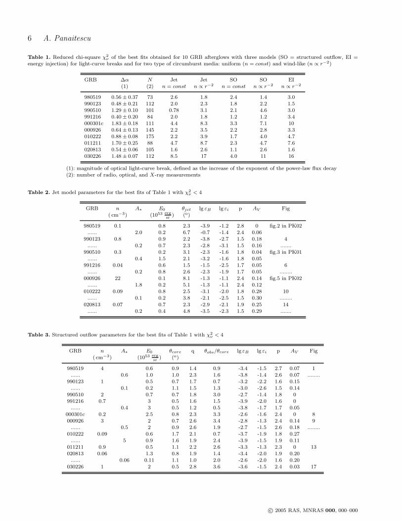
Table 1 lists the reduced chi-square, χ2ν , for the best fits ob-

tained with the Jet, SO, and EI models, for the two types ofcircumburst media: homogeneous and wind-like. For a uni-form CBM, the best fits with the EI model are very poorand, for almost all afterglows, they are substantially worsethan those for a wind. This is so because, for a uniformCBM, the observed post-break optical decay index α2 (givenby equation [6]) requires a higher electron index p than for awind, leading to an optical SED slope (βo) and an optical–to–X-ray spectral index (βox) larger than those observed.Also, the EI model has difficulties in accommodating boththe radio and X-ray fluxes, with the FS emission either over-estimating the observed radio flux or underestimating theX-ray flux.

Tables 2, 3, 4, and 5 list the parameters of the bestfits with χ2

ν < 4 for the Jet, SO, EI, and Jet+EI models,respectively, some of which are shown in Figs. 1–17. Fromthe parameter uncertainties determined by us (Panaitescu& Kumar 2002) for the Jet model from the χ2-variationaround its minimum for eight GRB afterglows, we estimatethe following uncertainties for the best fit parameters givenin Tables 2–5: σ(lgE0) = σ(lgEi) = 0.3, σ(lgn) = 0.7,σ(lgA∗) = 0.3, σ(θjet) = 0.3θjet, σ(θcore) = 0.2o, σ(lg εB) =1, σ(εi) = 0.3εi, σ(p) = 0.1, σ(q) = 0.3, σ(e) = 0.2, σ(AV ) =0.2AV .

Figs. 1–17 display the best fits obtained with theJet model for the afterglows 010222, 011211, 020813, and

three models and specific limits on the post-break light-curve de-cay indices which they yield.

c© 2005 RAS, MNRAS 000, 000–000

6 A. Panaitescu

Table 1. Reduced chi-square χ2ν of the best fits obtained for 10 GRB afterglows with three models (SO = structured outflow, EI =

energy injection) for light-curve breaks and for two type of circumburst media: uniform (n = const) and wind-like (n ∝ r−2)

GRB ∆α N Jet Jet SO SO EI(1) (2) n = const n ∝ r−2 n = const n ∝ r−2 n ∝ r−2

980519 0.56± 0.37 73 2.6 1.8 2.4 1.4 3.0990123 0.48± 0.21 112 2.0 2.3 1.8 2.2 1.5990510 1.29± 0.10 101 0.78 3.1 2.1 4.6 3.0991216 0.40± 0.20 84 2.0 1.8 1.2 1.2 3.4000301c 1.83± 0.18 111 4.4 8.3 3.3 7.1 10000926 0.64± 0.13 145 2.2 3.5 2.2 2.8 3.3010222 0.88± 0.08 175 2.2 3.9 1.7 4.0 4.7011211 1.70± 0.25 88 4.7 8.7 2.3 4.7 7.6020813 0.54± 0.06 105 1.6 2.6 1.1 2.6 1.6030226 1.48± 0.07 112 8.5 17 4.0 11 16

(1): magnitude of optical light-curve break, defined as the increase of the exponent of the power-law flux decay(2): number of radio, optical, and X-ray measurements

Table 2. Jet model parameters for the best fits of Table 1 with χ2ν < 4

GRB n A∗ E0 θjet lg εB lg εi p AV Fig( cm−3) (1053 erg

sr) (o)

980519 0.1 0.8 2.3 -3.9 -1.2 2.8 0 fig.2 in PK02...... 2.0 0.2 6.7 -0.7 -1.4 2.4 0.06

990123 0.8 0.9 2.2 -3.8 -2.7 1.5 0.18 4...... 0.2 0.7 2.3 -2.8 -3.1 1.5 0.16 .......

990510 0.3 0.2 3.1 -2.3 -1.6 1.8 0.04 fig.3 in PK01...... 0.4 1.5 2.1 -3.2 -1.6 1.8 0.05

991216 0.04 0.6 1.5 -1.5 -2.5 1.7 0.05 6...... 0.2 0.8 2.6 -2.3 -1.9 1.7 0.05 ........

000926 22 0.1 8.1 -1.3 -1.1 2.4 0.14 fig.5 in PK02...... 1.8 0.2 5.1 -1.3 -1.1 2.4 0.12

010222 0.09 0.8 2.5 -3.1 -2.0 1.8 0.28 10...... 0.1 0.2 3.8 -2.1 -2.5 1.5 0.30 ........

020813 0.07 0.7 2.3 -2.9 -2.1 1.9 0.25 14...... 0.2 0.4 4.8 -3.5 -2.3 1.5 0.29 .......

Table 3. Structured outflow parameters for the best fits of Table 1 with χ2ν < 4

GRB n A∗ E0 θcore q θobs/θcore lg εB lg εi p AV Fig( cm−3) (1053 erg

sr) (o)

980519 4 0.6 0.9 1.4 0.9 -3.4 -1.5 2.7 0.07 1...... 0.6 1.0 1.0 2.3 1.6 -3.8 -1.4 2.6 0.07 ........

990123 1 0.5 0.7 1.7 0.7 -3.2 -2.2 1.6 0.15...... 0.1 0.2 1.1 1.5 1.3 -3.0 -2.6 1.5 0.14

990510 2 0.7 0.7 1.8 3.0 -2.7 -1.4 1.8 0991216 0.7 3 0.5 1.6 1.5 -3.9 -2.0 1.6 0...... 0.4 3 0.5 1.2 0.5 -3.8 -1.7 1.7 0.05

000301c 0.2 2.5 0.8 2.3 3.3 -2.6 -1.6 2.4 0 8000926 3 2 0.7 2.6 3.4 -2.8 -1.3 2.4 0.14 9...... 0.5 2 0.9 2.6 1.9 -2.7 -1.5 2.6 0.18 ........

010222 0.09 0.6 1.7 2.1 0.7 -3.7 -1.9 1.8 0.27...... 5 0.9 1.6 1.9 2.4 -3.9 -1.5 1.9 0.11

011211 0.9 0.5 1.1 2.2 2.6 -3.3 -1.3 2.3 0 13020813 0.06 1.3 0.8 1.9 1.4 -3.4 -2.0 1.9 0.20...... 0.06 0.11 1.1 1.0 2.0 -2.6 -2.0 1.6 0.20

030226 1 2 0.5 2.8 3.6 -3.6 -1.5 2.4 0.03 17

c© 2005 RAS, MNRAS 000, 000–000

Jets, Structured Outflows, and Energy Injection in GRB Afterglows 7

Table 4. Best fit parameters obtained with the Energy Injection model

GRB n A∗ Ei e toff lg εB lg εi p AV Fig( cm−3) (1053 erg

sr) (day)

990123 0.003 0.08 0.7 0.5 -2.1 -1.0 2.3 0.04 5020813 0.13 0.7 0.3 0.9 -3.2 -2.5 1.8 0.22 15

Table 5. Best fit parameters obtained with the Jet+EI model

GRB χ2ν n A∗ E0 θjet Ei/E0 toff lg εB lg εi p AV Fig

( cm−3) (1053 ergsr

) (o) (day)

990123 1.9 10−3 0.9 2.0 0.1 0.7 -3.0 -1.2 2.3 0 3...... 2.5 0.04 0.7 6.0 0.2 0.7 -3.5 -1.3 1.8 0.06 .......

991216 2.2 10−3 1.4 2.1 0.1 1.5 -2.4 -1.1 2.4 0 7...... 1.6 0.04 0.8 3.6 0.2 1.8 -2.0 -1.5 2.0 0 ......

010222 1.6 10−4 0.7 2.0 0.06 2.5 -1.8 -1.3 2.3 0.19 11...... 3.6 0.06 0.4 5.0 0.6 1.7 -3.0 -1.7 1.7 0.19 ......

030226, which we did not present previously, and compara-ble or better fits obtained with the SO and EI models. Withthe exception of the Jet model and a uniform CBM for theafterglow 990510, all best fits presented are not acceptable ina statistical sense, as they have χ2

ν > 1. In general, fits withχ2ν < 4 appear adequate upon visual inspection, a significant

fraction of the χ2 arising often from optical measurements(which have the smallest uncertainties), indicating either asmall, short-lived afterglow fluctuation or, perhaps, an oc-casional outlier resulting from underestimated observationalerrors. In some cases there are also systematic discrepanciesbetween the model fluxes and observations, most often in theradio. As a general rule, if the fits are poorer than χ2 > 4for both types of circumburst media then the fits are notshown, with the exception of those obtained with the Jetand SO models for the afterglows 011211 and 030226, forwhich we want to show that the latter model is much betterthan the former in accommodating the 1 day, sharp opticallight-curve break. Also as a general rule, if the fits obtainedwith the Jet and SO models are comparable, only one isshown in the figures.

For clarity, the figures contain only the radio opticalfrequencies where observations span the longest time, butthe fitted data set included few or several other bands inthese two domains (see figure captions). With the exceptionof the afterglow 000926, the available X-ray measurementsare in only one band, which we use to infer the X-ray flux atthe mid energy of that band. The amplitude of interstellarscintillation, whose calculation is based on the treatmentand maps given by Walker (1998), is indicated with verticalbars at the time of the radio observations. In all figures, thebest fit for a uniform CBM is shown with continuous lineswhile that for a wind medium with dotted lines.

3.1 980519

The best fit obtained with the Jet model is discussed inPanaitescu & Kumar (2002). The addition of more radiodata and some optical outliers (which were previously ex-cluded) lead now to a worse fit (χ2-wise) but to the same

afterglow parameters, within their uncertainty. The best fitfor the SO model, shown in Fig. 1, has a χ2

ν comparable tothat for the Jet model (Table 1) but is qualitatively poorer,as it overestimates the observed early radio. Although themeasured radio fluxes are within the amplitude of the fluc-tuations caused by the interstellar Galactic gas, such a con-stant offset cannot be caused by scintillation (unfortunately,χ2-statistics does not reflect the smaller probability of sys-tematic discrepancies).

3.2 990123

The best fit obtained with the Jet model and a uniformmedium is presented in Panaitescu & Kumar (2001). Therewe assumed that the radio flare seen at 1 day (Kulkarni etal. 1999) arises in the GRB ejecta energized by the RS, andincluded in the modelling only the radio measurements at 3–30 days, when the 8 GHz flux of this afterglow is less than40µJy. This sets an upper limit on the FS peak flux, Fp,which, together with that Fp ∝ n1/2 before the jet-breakand Fp ∝ n1/6 after that, requires a small CBM density:n < 10−2 cm−3.

Including the radio measurements before a few days,as well as the millimeter data, the K-band fluxes after 10days (with which the K-band light-curve appears to be asingle power-law, unlike theR-band emission, which exhibitsa steepening at ∼ 2 days), and other optical measurementspreviously left out of our modelling, we find now a poorerfit (χ2

ν = 2.4 for a uniform CBM, χ2ν = 5.1 for a wind), but

with the same afterglow parameters as before.We have also tested the ability of the Jet model includ-

ing the emission from the RS crossing the GRB ejecta toexplain the optical flash observed at 20–600 seconds (Ak-erlof et al. 1999), which peaked 50 s after the burst at about0.8 Jy, and the 1 day radio flare, as proposed by Sari &Piran (1999). Given that the observer injection timescale(∼ 100 s) is comparable to the burst duration, the approx-imation of instantaneous ejecta release and its consequencegiven in equation (13) may be invalid. For this reason, we letthe ejecta Lorentz factor, Γi, to be a free parameter of the

c© 2005 RAS, MNRAS 000, 000–000

8 A. Panaitescu

fit. Together with the injected energy, Ei, it determines thenumber of the radiating electrons in the GRB ejecta and theLorentz factor of the RS, i.e. the peak flux and frequency ofthe synchrotron RS emission.

The best fits obtained with the Jet model interactingwith a tenuous medium (so that the FS emission accommo-dates the late radio measurements) and emission from theGRB ejecta are shown in Fig. 2. We find that, for the samemicrophysical parameters εi and εB behind both shocks, thepeak RS optical emission is dimmer than observed by a fac-tor 50 for a uniform CBM and a factor 5 for a wind, thelatter yielding a good fit to the remainder of the early op-tical measurements (but not as good as a uniform mediumto the 1 day optical break). We also find that, under thesame assumption of equal microphysical parameters, the RSemission peaks at 8 GHz at 0.1 day, i.e. a factor 10 tooearly. In other words, taking into account the cooling of theRS electrons accelerated at ∼ 100 s and the decrease on thesynchrotron self-absorption optical thickness of the RS atradio frequencies, we do not find a set of afterglow parame-ters for which the RS emission can peak in the radio as latea 1 day while, for the same microphysical parameters, theFS emission can accommodate the rest of afterglow obser-vations. To explain the optical flash of the afterglow 990123,the GRB ejecta must have a larger parameter εB than forthe forward shock, indicating that the ejecta is magnetized(Zhang, Kobayashi & Meszaros 2003, Panaitescu & Kumar2004), a feature that may be required for by the early op-tical emission of the afterglow 021211 as well (Kumar &Panaitescu 2003, Zhang et al. 2003).

However, for the low density Jet model, an injection ofejecta in the FS at about the same time when the radioflare is seen allows this model to accommodate that flare,as shown in Fig. 3. Note that the injected energy is lessthan that required for the FS to explain the rest of theobservations, i.e. the incoming ejecta provide only the freshelectrons to radiate at radio frequencies, but do not alterthe dynamics of the FS.

After including the 1 day radio flare measurements, aswell as the millimetre measurements at 1–10 days, we alsofind with the Jet model a higher density solution (Fig. 4),n <∼ 1 cm−3, which is close to that obtained for other af-

terglows. This higher density¶is required by the larger FSpeak flux necessary to accommodate the 1 day flare, whenF8GHz = 0.36 mJy. For a uniform CBM, the high densityfit is slightly better than the low density solution, the im-provement being more substantial for a wind. Note, however,that the former underestimates the radio measurements at30 days.

The SO model yields fits of the same quality as the Jetmodel (Table 1). The best fit structural parameter satisfiesq > q(p) for a uniform medium and q < q(p) for a wind (Ta-ble 3), thus the post-break afterglow emission arises mostly

¶ It also lowers the cooling frequency, νc, to just slightly abovethe (blueward of) optical domain, which requires a hard electrondistribution with index p >∼ 2βox ≃ 4/3. Furthermore, a lowelectron parameter εi is required for the FS peak frequency toreach 10 GHz as early as 1 day after the burst, and to explain theradio flare

from the outflow core in the former case and from the enve-lope for the latter.

The best fit obtained with the EI model for a windmedium is shown in Fig. 5. χ2-wise, this low density modelprovides a better fit than the Jet and SO models, althoughit overestimates the early radio measurements. Also, this so-lution has an extremely low wind density (Table 4), about100 times smaller than known for Galactic WR stars. Forsuch a tenuous wind, equation (5) implies that, if the out-flow opening θjet is wider than 2o, then the jet-break wouldappear later than about 30 days (i.e. after the latest mea-surement), and the corresponding outflow energy would belarger than 2 × 1050 ergs, which is less than that of the jetshown in Fig. 4. The best fit obtained for a uniform mediumis very poor (it either overestimates the radio emission orunderproduces X-rays) and is not shown.

3.3 990510

The best with the Jet model for a uniform CBM is shownin Panaitescu & Kumar (2001). A wind provides a poorerfit (Table 1), as it fails to accommodate the strong breakof the optical light-curves of this afterglow. Structured out-flows yield poorer fits for either type of medium, the best fitstructural parameter being q = 1.8 for a uniform CBM andq = 1.4 for a wind.

3.4 991216

The best fit obtained with the Jet model and a uniformCBM is shown in Panaitescu & Kumar (2001). Because theradio decay of this afterglow, F8GHz ∝ t−0.77±0.06, is sig-nificantly slower than that measured at optical wavelengthsafter the break, Fo ∝ t−1.65±0.12, in our previous modellingwe have employed a double power-law electron distribution,harder (smaller index p) at low energies, to accommodatethe shallower radio decay, and a softer (larger index p) athigh energies, to explain the post-break optical light-curvedecay.

Here we use a single power-law electron distribution, toassess the ability of each model to explain all the data with-out recourse to a light-curve decay steepening originatingin a break in the electron distribution. Consequently, theJet model (as well as any other single emission componentmodel) will not accommodate the decays of both the radioand optical emissions of the afterglow 991216, as illustratedby the higher χ2

ν given in Table 1 and the best fit shown inFig. 6.

The addition of emission from the RS which energizesthe ejecta catching up with the FS at about 1 day improvesthe radio fit, as shown in Fig. 7. A slower decay radio light-curve is obtained as the FS emission overtakes that from theRS at about 10 days. As for the afterglow 990123 (Fig. 3),the energy injected is small enough that it does not alterthe dynamics of the FS. However, the afterglow parametersof the Jet+EI model for 991216 are different than those ob-tained with the Jet model (Fig. 6) because we require nowthat the FS peaks in the radio at a later time and at a lower

flux (∼ 0.1 mJy)‖.

‖ This requires a tenuous CBM, which increases the cooling fre-

c© 2005 RAS, MNRAS 000, 000–000

Jets, Structured Outflows, and Energy Injection in GRB Afterglows 9

The SO model yields a best fit which is very similar tothat shown in Fig. 6 for the Jet model. The smaller intensity-averaged source size resulting in the SO model leads to alarger amplitude for the interstellar scintillation and, thus,to a better χ2-wise fit (Table 1), but this model also fails toaccommodate the slow radio decay. The best fit structuralparameter satisfies q <∼ q(p) (Table 3), i.e. the outflow en-velope emission dominates over that from the core after theoptical break.

3.5 000301c

The best fit for the Jet model is discussed in Panaitescu(2001). As for the afterglow 991216, the slower radio decayof 000301c, F8GHz ∝ t−1.1±0.3, and its faster optical fall-off,Fo ∝ t−2.83±0.12, prompted us to consider a double power-law electron distribution. Furthermore, the large break mag-nitude ∆α = 1.8 ± 0.2 exhibited by the optical light-curve000301c (the largest in the entire sample - Table 1) exceedsthat allowed by the Jet model for the electron distributionindex p required by the pre-break decay index and opticalSED slope (Panaitescu 2005). Such a strong break is alsobetter explained if there is a contribution from the passageof a spectral break. However, since we want to test the threemodels for light-curve break without any contribution fromanother mechanism, we list in Table 1 the best fit obtainedpreviously with a soft electron distribution.

Fig. 8 shows the best fit obtained with the SO model,which is only slightly better than that of the Jet model, hassimilar parameters, and shares the same deficiencies: it failsto explain the sharpness of the optical light-curve break andyields a radio emission decaying faster than observed. Wenote that optical measurements between 3.0 and 4.5 days,when a light-curve bump is seen, have been excluded fromthe fit.

3.6 000926

The best fit obtained with the Jet model is shown inPanaitescu & Kumar (2002). After including in the data setthe near-infrared measurements, the noisy I-band, and someoptical outliers which were previously excluded, the best fitis χ2-wise poorer but the fit parameters are the same as be-fore (within their uncertainty). An equally good fit can beobtained with the SO model (Fig. 9). We note that for boththe Jet and S0 models, the X-ray emission is mostly inverseCompton scatterings.

3.7 010222

The best fit obtained with the Jet model is shown in Fig.10. Note that the model radio light-curve decays after 1 day

quency (νc ∝ n−1 before the jet-break and νc ∝ n−5/6 afterthat). Going from the Jet fit to the Jet+EI fit increases the cool-

ing frequency from about 1015 Hz to 3 × 1017 Hz. Then, to ac-commodate the optical–to–X-ray SED slope, the Jet+EI modelrequires a softer electron distribution than the Jet model, whichin turn yields a faster post-break decay of the afterglow light-curve, as shown in Fig. 7, and a poorer fit to the optical emissionafter 10 days

faster than observed. For a uniform CBM, the best fit ob-tained with a structured outflow is slightly better in theradio, but it too fails to explain the slow radio decay. Fora wind, the best fit obtained with the SO model overesti-mates the millimeter emission [F250GHz(1 − 100 d) ≃ 1.2mJy, F350GHz(0.3− 20 d) ≃ 3.9 mJy] attributed to the hostgalaxy by Frail et al. (2002), who also suggest a possiblehost synchrotron emission at 8.5 GHz of ∼ 20 µJy. Thisis only marginally consistent with the F1.4GHz(447 d) =−1 ± 35µJy reported by Galama et al. (2003) and thehost synchrotron SED, Fν ∝ ν−0.75, adopted by Frail etal. (2002), which imply a host flux F8GHz = 0± 9 µJy.

If we subtract a radio host contribution of F(host)ν =

20 (ν/8GHz)−0.75 µJy from the 44 radio measurements,then, within the Jet model, the contribution to χ2 of theradio data decreases from 107 to 72 for a uniform medium,and from 103 to 53 for a wind, with similar changes forthe SO model. Though these are significant improvements,the best fit still underestimates the radio flux measuredafter 10 days, because the optical measurements have asmaller uncertainty and determine the electron index p and,implicitly, the decay of the model radio emission. In gen-eral, one-component models cannot accommodate both thehost-subtracted radio emission, F8GHz ∝ t−0.76±0.12, ofthe afterglow 010222 at 1–200 days, and the optical decay,Fo ∝ t−1.78±0.08, observed at 10–100 days.

A better fit to the radio emission of the afterglow 010222may be obtained with the Jet model if, in addition to theFS emission, there is a RS contribution to the early radioafterglow, as illustrated in Fig. 11 for a uniform CBM. Justas for the afterglows 990123 and 991216, the incoming ejectacarry less energy than that in the FS (and do not alter itsdynamics) and the medium density is lower than for theJet model because the FS peak flux must be smaller, tomatch the radio flux measured after 10 days, when the FSsynchrotron peak frequency crosses the radio domain.

3.8 011211

As illustrated in Fig. 12, even for a uniform CBM, the Jetmodel has difficulty in accommodating the sharp break ex-hibited by the optical light-curve of this afterglow, assum-ing that the 1–2 day optical emission is not a fluctuation.Such fluctuations have been seen in the afterglows 000301c,021004, and 030329, but the lack of a continuous monitoringfor 011211 prevents us to determine if its optical emission at1 day is indeed a fluctuation. A stronger break can be ob-tained with the SO model when the brighter, outflow corebecomes visible to an observer located outside it, hence thebetter fit that the SO model yields (Fig. 13).

3.9 020813

The best fit obtained with the Jet model is shown in Fig.14. Structured outflows yield fits with q > q(p) for a uni-form CBM and q < q(p) for a wind, i.e. with the post-breakemission arising mostly in the outflow core and envelope,respectively. A significant improvement over the Jet modelis obtained only for a uniform CBM (Table 1).

A fit of comparable quality is also obtained with the

c© 2005 RAS, MNRAS 000, 000–000

10 A. Panaitescu

EI model for a wind medium (Fig. 15), but not for a uni-form CBM, which overproduces radio emission and largelyunderestimates the observed X-ray fluxes. For the best fitparameters given in Table 4, equation (5) shows that a jet-break would occur after the last measurement (40 days) ifthe outflow opening were larger than 5o, which implies aminimum collimated energy of 2×1051 ergs, which is 3 timeslarger than that of the jet shown in Fig. 14. Therefore, justas for 990123, the EI model may not involve significantlylarger energies than the Jet model, if allowance is made fora possible outflow collimation.

3.10 030226

As for 011211, the strong optical light-curve break of thisafterglow is better accommodated by the SO model thanthe Jet model (Fig. 16 and 17), though an acceptable fit tothe optical break is obtained only for a uniform CBM (inaddition, for a wind medium, the SO model overproducesradio emission). However, given the poor coverage before0.3 days, it is possible that the measured optical emissionat that time is a fluctuation below that expected in the Jetmodel.

3.11 970508

Although the decay of the optical emission of this afterglowdoes not exhibit a steepening, being so far the longest mon-itored power-law fall-off (2–300 days), it can be explainedwith the Jet model if its unusual rise at 1–2 days is inter-preted as a jet becoming visible to an observer located out-side the initial jet opening (see fig. 1 in Panaitescu & Kumar2002). This requires a rather wide jet, with θjet = 18o, andyields a poor fit to the X-ray emission (χ2

ν = 2.8). A lessenergetic envelope surrounding this jet would produce theprompt γ-ray emission and would account for the flat opti-cal emission prior to the 2 day optical rise, hence this modelis similar to a Structured Outflow with a wide uniform coreand an envelope whose structure is poorly constrained byobservations.

An other possible reason for the 2 day sharp rise of thisafterglow is a powerful energy injection episode in which theincoming ejecta carry an energy larger than that alreadyexisting in the FS (Panaitescu, Meszaros & Rees 1998), i.e.the blast-wave dynamics is altered drastically by the energyinjection. Fig. 18 shows the best with the EI model. Notethat the given that the light-curve rise is achromatic, as itarises from the blast-wave dynamics, which explains why theX-ray light-curve cannot be accommodated.

4 CONCLUSIONS

In this work we expand our previous investigation(Panaitescu & Kumar 2003) of the Jet model to four otherGRB afterglows for which an optical light-curve break wasobserved: 010222 (for which radio observations were notavailable at the time of our previous modelling), 011211,020813, and 030226. We also note that, here, we have notemployed a broken power-law electron distribution to ex-plain both the slower decaying radio emission and the faster

falling-off optical light-curve observed for some afterglows(e.g. 991216 and 000301c).

Our prior conclusion that a homogeneous circumburstmedium provides a better fit to the broadband afterglowemission than environments with a wind-like stratificationstands (Table 1). For afterglows with a sharp steepening ∆αof the optical light-curve decay (990510, 000301c, 011211,and 030226), this is due to that the transition between thejet asymptotic dynamical regimes (spherical expansion atearly times and lateral spreading afterward) occurs fasterfor a homogeneous medium than for a wind (Kumar &Panaitescu 2000). For the afterglows with shallower breaks,a wind medium (as expected if the GRB progenitor is a mas-sive star) provides an equally good fit as (or, at least, notmuch worse than) a homogeneous medium.

For the acceptable fits (Table 2) obtained with the Jetmodel and for a uniform medium, the jet initial kinetic en-ergy, Ejet, is between 2 and 6 ×1050 ergs, the initial jetopening angle, θjet, is between 2o and 3o (with 000926 anoutlier at 8o), and the medium density, n, between 0.05 and1 cm−3 (with 000926 an outlier, again, at 20 cm−3). Fora wind, Ejet has about the same range, θjet ranges from2o to 6o, while the wind parameter A∗ is between 0.1 and2. 70% of the 64 Galactic WR stars analyzed by Nugis &Lamers (2000) have a A∗ parameter in this range; for therest A∗ ∈ (2, 5). We note that the Ejet resulting from ournumerical fits is uncertain by a factor 2, θjet by about 30%,n by almost one order of magnitude, and A∗ by a factor of2.

Although the inferred wind density parameter A∗ isin accord with the measurements for WR stars a uniformmedium is instead favoured by the fits to the afterglow data.This is an interesting issue for the established origin of longbursts in the collapse of massive stars. Wijers (2001) hasproposed that the termination shock resulting from the in-teraction between the wind and the circumstellar mediumcould homogenize the wind. The numerical hydrodynamicalcalculations of Garcia-Segura, Langer & Mac Low (1996)show that, for a negligible pressure nT of the circumstel-lar medium (about 104 cm−3K), the termination shock ofthe RSG wind has a radius of 10 pc, outside a shell of uni-form density is form. However, this radius is much largerthan the distance of about 1 pc where the afterglow emis-sion is produced. Chevalier, Li & Fransson (2004) made thecase that, if the burst occurred in an intense starburst re-gion, where the interstellar pressure is about 107 cm−3K,then the shocked RSG wind would form bubble of uni-form density of about 1 cm−3 extending from 0.4 to 1.6pc, in accord with the fit densities and the blast-wave ra-dius r = 8cΓ2t/(1+ z) = 0.5 (E0,53/n0)

1/4[td/(1+ z)]1/4 pc,resulting from equation (2).

The Structured Outflow model involving an ener-getic, uniform core, surrounded by a power-law envelope(equation [7]) which impedes the lateral spreading of thecore, retains most of the ability of the Jet model to yielda steeply decaying optical light-curve after the core (or itsboundary) becomes visible to an observer located outsidethe core opening (or within it), while accommodating, atthe same time, the observed slope of the optical spectralenergy distribution (SED). This is so because, in both mod-els, more than half of the increase ∆α in the light-curvepower-law decay index is due to the finite opening of the

c© 2005 RAS, MNRAS 000, 000–000

Jets, Structured Outflows, and Energy Injection in GRB Afterglows 11

bright(er) ejecta. For a jet, the remainder of the steepening∆α is caused by the lateral spreading. For a structured out-flow, an extra contribution to the steepening, which can leadto a ∆α even larger than that produced by a jet, results ifthe observer is located outside the core opening.

For a uniform medium, we find that the Structured Out-flow model provides a better fit than the Jet model for 6of the 10 afterglows analyzed here (Table 1). For a wind,the former model works better for three afterglows, fits ofcomparable quality being obtained for the other six. Onlythe afterglow 990510 is better explained with a jet, for ei-ther type of circumburst medium. Within the framework ofstructured outflows, 8 out of 10 afterglows are better fit witha uniform medium than with a wind, which is partly due tothat, just as for a jet, the light-curve steepening is sharperif the medium is uniform (Panaitescu & Kumar 2003).

For the ”acceptable” fits (χ2ν < 4) obtained with the

SO model, the ejecta kinetic energy per solid angle in thecore, E0, ranges from 0.5 to 3 ×1053 ergs sr−1 for either typeof medium, with an uncertainty of a factor 3. The angularopening of the core, θcore, is between 0.5o and 1o for a ho-mogeneous medium, and about 1o for a wind (991216 be-ing an outlier at 0.5o), with an uncertainty less than 50%.The structural parameter q (equation [7]), which character-izes the energy distribution in the outflow envelope, is foundto be between 1.5 and 2.7 for a uniform medium, and be-tween 1.0 and 2.3 for a wind (with 000926 being an outlierat 2.9). These values are consistent with that proposed byRossi et al. (2002), q = 2, to explain the quasi-universaljet energy resulting in the Jet model. For structured out-flows, the ejecta kinetic energy contained within an openingof twice the location of the observer (relative to the outflowsymmetry axis), θobs, ranges from 1 to 4 ×1050 ergs, for ei-ther type of medium. Hence, the energy budget required bythe Structured Outflow model is very similar to that of theJet model. The best fit medium densities obtained with theStructured Outflow model are similar to those resulting fora Jet.

We find that the Energy Injection model, where alight-curve decay steepening is attributed to the cessation ofenergy injection in the forward shock, can be at work only intwo afterglows, 990123 and 020813. The major shortcomingof the EI model is that, in order to explain the steep fall-offof the optical light-curve after the break with a sphericaloutflow, an electron distribution that is too soft (i.e. an in-dex p too large) is required to accommodate the relativeintensities of the radio and X-ray emissions. Low densitysolutions (n < 1 cm−3, A∗ < 0.1), for which the X-ray emis-sion is mostly synchrotron, yield a cooling frequency thatis too low, resulting in model X-ray fluxes underestimatingthe observations by a factor of at least 10. High density solu-tions (n > 10 cm−3, A∗ > 1), for which the X-ray is mostlyinverse Compton scatterings, produce a forward shock peakflux that is too large, which leads to model radio fluxes over-estimating the data by a factor of 10.

We note that, due to adiabatic cooling, the GRB ejectaelectrons which were energized by the reverse shock duringthe burst, do not contribute significantly to the afterglowradio emission at days after the burst. Numerically, we findthat, if the microphysical parameters are the same for boththe reverse and forward shocks, then the 1 day radio flareof the afterglow 990123 cannot be explained with the emis-

sion from the GRB ejecta electrons, as proposed by Sari &Piran (1999), as the synchrotron emission from these elec-trons peaks in the radio earlier than 0.1 day, regardless ofhow relativistic is the reverse shock. For the reverse shockemission to be significant at 1 day after the burst, there mustbe some other ejecta catching up with the decelerating out-flow at that time or the assumption of equal microphysicalparameters for both shocks must be invalid (Panaitescu &Kumar 2004). Furthermore, the optical emission from theejecta electrons is below that observed at 100 s (Akerlof etal. 1999) by a factor 5 for a wind and a factor 50 for auniform medium.

A delayed injection of ejecta, carrying less kinetic en-ergy than that already existing in the forward shock (i.e.not altering the forward shock dynamics), may be at workin the afterglows 990123, 991216, and 010222, whose radiodecay is substantially slower than that observed in the op-tical after the break. As shown by us (Panaitescu & Kumar2004), such a decoupling of the radio and optical emissionscannot be explained by models based on a single emissioncomponent (forward shock) and require the contribution ofthe reverse shock. Figs. 3, 7, and 11, illustrate that the sumof the reverse and forward shock emissions yields a slowerdecaying radio emission, consistent with the observations.However, for the forward shock peak flux to be as dim asobserved in the radio after 10 days, when the forward shockpeak frequency decreases to 10 GHz, an extremely tenuousmedium is required: n ∼ 10−3 cm−3 or A∗ ∼ 0.05. The for-mer might be compatible with a massive star progenitor ifGRBs occur in the ”superbubble” blown by preceding su-pernovae exploding in the same molecular cloud (Scalo &Wheeler 2001), while the latter points to a progenitor witha low mass and low metallicity or, otherwise, to a small mass-loss rate and high wind speed during the last few thousandyears before the collapse, when the environment within 1 pcis shaped by the stellar wind.

As a final conclusion, we note that the Structured Out-flow model is a serious contender to the Jet model in accom-modating the broadband emission of GRB afterglows withoptical light-curve breaks. In both models, the best fit pa-rameters describing the ejecta kinetic energy – jet opening& energy or core opening & energy density along the out-flow symmetry axis – have narrow distributions, hinting toa possible universality of these parameters.

ACKNOWLEDGMENTS

This work was supported by NSF grant AST-0406878.

Some or all of the radio data for the afterglows 011211, 020813,

and 030226 referred to in this paper were drawn from the GRB

Large Program at the VLA

(http://www.vla.nrao.edu/astro/prop/largeprop) and can be

found at Dale Frail’s website

http://www.aoc.nrao.edu/∼dfrail/allgrb table.shtml .

c© 2005 RAS, MNRAS 000, 000–000

12 A. Panaitescu

REFERENCES

Akerlof C. et al. , 1999, Nature, 398, 400

Berger E. et al. , 2000, ApJ, 5454, 56

Bertoldi F. et al. , 2003, GCN Circ. 1497(http://gcn.gsfc.nasa.gov/gcn3/1497.gcn3)

Borozdin K., Trodolybov S., 2003, ApJ, 583, L57

Bremer M. et al. , 1998, A&A, 332, L13

Butler N. et al. , 2003, ApJ, 597, 1010

Chary R. et al. , 1998, 498, L9

Chevalier R., Li Z., 2000, ApJ, 536, 195

Chevalier R., Li Z., Fransson C., 2004, ApJ, 606, 369

Corbet R., 1999, GCN Circ. 506(http://gcn.gsfc.nasa.gov/gcn3/506.gcn3)

Covino S. et al. , 2003, A&A, 404, L5

Fox D. et al. , 2003, Nature, 422, 284

Frail D., Waxman E., Kulkarni S., 2000a, ApJ, 537, 191

Frail D. et al. , 2000b, ApJ, 534, 559

Frail D. et al. , 2000c, ApJ, 538, L129

Frail D. et al. , 2002, ApJ, 565, 829

Frail D. et al. , 2003, AJ, 125, 2299

Frail D. et al. , 2005, ApJ, 619, 994

Fynbo J. et al. , 2001, A&A, 373, 796

Galama T. et al. , 1998, ApJ, 497, L13

Galama T. et al. , 1999, Nature, 398, 394

Galama T. et al. , 2000, ApJ, 541, L45

Galama T. et al. , 2003, ApJ, 587, 135

Garcia M. et al. , 1998, ApJ, 500, L105

Garcia-Segura G., Langer N., Mac Low M., 1996, A&A, 316, 133

Garnavich P. et al. , 2000, ApJ, 543, 61

Goodman J., 1997, New Astronomy, 2, 449

Gorosabel J. et al. , 2004, A&A, 422, 113

Granot J., Piran T., Sari R., 1999, ApJ, 527, 236

Granot J., Panaitescu A., Kumar P., Woosley S., 2002, ApJ, 570,L61

Halpern J. et al. , 1999, ApJ, 517, L105

Halpern J. et al. , 2000, ApJ, 543, 697

Harrison F. et al. , 2001, ApJ, 559, 123

Holland S. et al. , 2002, ApJ, 124, 639

in’t Zand J. et al. , 2001, ApJ, 571, 876

Jakobsson P. et al. , 2001, A&A, 408, 941

Jaunsen, A. et al. 2001, ApJ, 546, 127

Jensen B. et al. , 2001, A&A 370, 909

Klose S. et al. , 2004, AJ, 128, 1942

Kulkarni S. et al. , 1999, Nature, 398, 394

Kumar P., Panaitescu A., 2000, ApJ, 541, L9

Kumar P., Panaitescu A., 2003, MNRAS, 346, 905

Masetti N. et al. , 2001, A&A, 374, 382

Meszaros P., Rees M.J., 1997, ApJ, 476, 232

Meszaros P., Rees M.J., Wijers R., 1998, ApJ, 499, 301

Nicastro L. et al. , 1999, A&A, 138, S437

Nugis T., Lamers H., 2000, A&A, 360, 227

Paczynski B., 1998, ApJ, 494, L45

Paczynski B., Rhoads J., 1993, ApJ, 418, L5

Pandey S. et al. , 2004, A&A, 417, 919

Panaitescu A., 2001, ApJ, 556, 1002

Panaitescu A., 2004, MNRAS, 350, 213

Panaitescu A., 2005, MNRAS, in press(http://xxx.lanl.gov/ps/astro-ph/0506577)

Panaitescu A., Kumar P., 2000, ApJ, 543, 66

Panaitescu A., Kumar P., 2001, ApJ, 554, 667 (PK01)

Panaitescu A., Kumar P., 2002, ApJ, 571, 779 (PK02)

Panaitescu A., Kumar P., 2003, ApJ, 592, 390

Panaitescu A., Kumar P., 2004, MNRAS, 353, 511

Panaitescu A., Meszaros P., Rees M., 1998, ApJ, 503, 314

Pedersen H. et al. , 1998, ApJ, 496, 311

Pei Y., 1992, ApJ, 395, 130

Piro L., 2000, preprint(http://xxx.lanl.gov/ps/astro-ph/0001436)

Piro L. et al. , 1998, A&A, 331, L41Piro L. et al. , 1999, GCN Circ. 500

(http://gcn.gsfc.nasa.gov/gcn3/500.gcn3)Piro L. et al. , 2001, ApJ, 558, 442Price P. et al. , 2001, ApJ, 549, L7Rees M.J., Meszaros P., 1998, ApJ, 496, L1Rhoads J., 1999, ApJ, 525, 737Rhoads J., Fruchter A., 2001, ApJ, 546, 117Rossi E., Lazzati D., Rees, M.J., 2002, MNRAS, 332, 945Sahu K. et al. , 1997, ApJ, 489, L127Sari P., Piran T., 1999, ApJ, 517, L109

Sari P., Meszaros P., 2000, ApJ, 535, L33Sari R., Narayan R., Piran T., 1998, ApJ, 497, L1Sari, R., Piran, T., Halpern J., 1999, ApJ, 519, L17Scalo J., Wheeler J, 2001, ApJ, 562, 664Smith I. et al. , 2001, A&A, 380, 81Sokolov V. et al. , 1998, A&A, 334, 117Stanek K. et al. , 2001, ApJ, 563, 592Takeshima T., 1999, GCN Circ. 478

(http://gcn.gsfc.nasa.gov/gcn3/478.gcn3)Vrba F. et al. , 1999, ApJ, 528, 254Walker M., 1998, MNRAS, 294, 307Waxman E., Kulkarni S., Frail D., 1998, ApJ, 497, 288Wijers R., Galama T., 1999, ApJ, 523, 177Wijers R., 2001, Proc. of Second Rome Workshop ”GRBs in

the Afterglow Era”, eds. E. Costa, F. Frontera, J. Hjorth(Berlin:Springer), 306

Woosley, S. 1993, ApJ, 405, 273Zhang B., Meszaros P., 2002, ApJ, 571, 876Zhang B., Kobayashi S., Meszaros P., 2003, ApJ, 595, 950

c© 2005 RAS, MNRAS 000, 000–000

Jets, Structured Outflows, and Energy Injection in GRB Afterglows 13

10−1 100 101 102

time (day)

10−6

10−5

10−4

10−3

10−2

10−1

100

101

Fν

(mJy

)

unif CBMwind

0519.jo

8.5 GHz

5 keV

I

Figure 1. Best fit for the afterglow 980519 with the SO model.The data set contains measurements at 1.4, 4.9, 8.5, 100 GHz(Frail et al. 2000b), I, R, V, B, U bands (Halpern et al. 1999, Vrbaet al. 2000, Jaunsen et al. 2001), and 5 keV (inferred from the 2–10 keV fluxes presented by Nicastro et al. 1999). Vertical barson the model radio light-curve indicate the amplitude of Galacticinterstellar scintillation. The model X-ray emission is mostly in-verse Compton scatterings. For this afterglow, a redshift was notmeasured. We assumed z = 1.

10−4 10−3 10−2 10−1 100 101 102

time (day)

10−5

10−4

10−3

10−2

10−1

100

101

102

103

Fν (

mJy

)

unif CBMwind

0123jet+rs

8.3 GHz (x100)

6 keV

R band

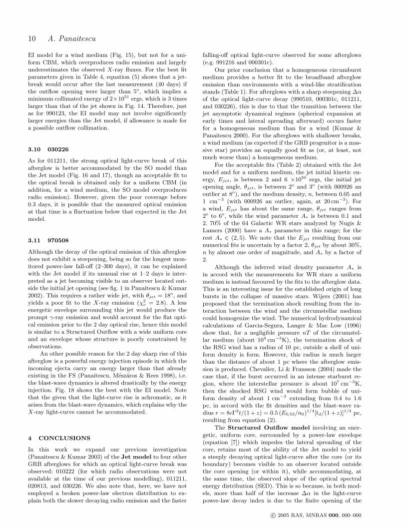
Figure 2. Best fit for the afterglow 990123 with the Jet modeland emission from the ejecta electrons accelerated by the reverseshock during the burst (t ≃ 100 s). The data set contains mea-surements at 1.4, 4.9, 8.3, 15, 86, 353 GHz (Galama et al. 1999,Kulkarni et al. 1999), K, H, I, R, V, B (Akerlof et al. 1999,Galama et al. 1999, Kulkarni et al. 1999), and 6 keV (inferredfrom the 2–10 keV fluxes reported by Piro 2000). Triangles de-note 2σ observational limits on the 8.3 GHz emission. Radio fluxeshave been shifted upwards by a factor 100, for clarity. For thismodel, the ejecta Lorentz factor Γi was not constrained by equa-tion (13), because the assumption of instantaneous ejecta releasemay not be valid, and was left a free parameter. The opticalpeak at 100 s and the radio flux before 1 day represent the re-verse shock emission, which is later overshined by the forwardshock. Model parameters are: E0 = 3×1050ergs sr−1, θjet = 2.2o,n = 0.004 cm−3, Ei = 1.3× 1053ergs sr−1, Γi = 5, 000, toff = 90s, εB = 4 × 10−4, εi = 0.075, p = 2.2, AV = 0.08 for a uniformmedium and E0 = 1.5 × 1050ergs sr−1, θjet = 6.0o, A∗ = 0.06,Ei = 3×1053ergs sr−1, Γi = 1, 200, toff = 170 s, εB = 7×10−5,εi = 0.080, p = 2.1, AV = 0.07 for a wind. The addition of theearly optical data has worsened the fits: χ2

ν = 14 for the formermedium, χ2

ν = 11 for the latter. Note that the wind model ac-commodates most of the early optical observations but, for eithertype of medium, the reverse shock emission peaks in the radio tooearly, at about 0.1 day.

c© 2005 RAS, MNRAS 000, 000–000

14 A. Panaitescu

10−1 100 101

time (day)

10−5

10−4

10−3

10−2

10−1

100

Fν

(mJy

)

unif CBMwind

0123.jet+ei

8.3 GHz

6 keV

R

Figure 3. Best fit for the afterglow 990123 with the Jet+EImodel for a uniform medium and a wind. The peak of the radiolight-curve before 1 day represents the reverse shock emission,while the forward shock peak frequency crosses the radio domainafter 10 days.

10−1 100 101

time (day)

10−5

10−4

10−3

10−2

10−1

100

Fν

(mJy

)

unif CBMwind0123.jet

8.3 GHz

6 keV

R

Figure 4. Best fit for the afterglow 990123 with the Jet model.Note that, in contrast to the fits shown in figure 3, the mediumdensity of these fits is similar to that determined for other af-terglows. However, the electron energy distribution has unusualparameters εi and p.

10−1 100 101

time (day)

10−5

10−4

10−3

10−2

10−1

100

Fν (

mJy

)

wind CBM

0123.ei

8.3 GHz

6 keV

R

Figure 5. Best fit for the afterglow 990123 with the EI model fora wind medium. The model radio emission until 10 days arises inthe reverse shock which has energized the incoming ejecta, afterwhich the forward shock emission overtakes it.

10−1 100 101 102

time (day)

10−4

10−3

10−2

10−1

100

Fν (

mJy

)

unif CBMwind1216.jet

8.5 GHz

6 keV

R

Figure 6. Best fit for the afterglow 991216 with the Jet model.The data set consists of measurements at 1.4, 4.9, 8.5, 15 GHz(Frail et al. 2000c), K,H, J, I,R, V bands (Garnavich et al. 2000,Halpern et al. 2000), and 6 keV (inferred from the 2–10 keV fluxesreported by Corbet & Smith 1999, Piro et al. 1999, Takeshima etal. 1999). Note that this model cannot explain the slower radiodecay observed at about the same time with the faster opticalfall-off.

c© 2005 RAS, MNRAS 000, 000–000

Jets, Structured Outflows, and Energy Injection in GRB Afterglows 15

10−1 100 101 102

time (day)

10−4

10−3

10−2

10−1

100

Fν

(mJy

)

unif CBMwind1216.jet+ei

8.5 GHz

6 keV

R

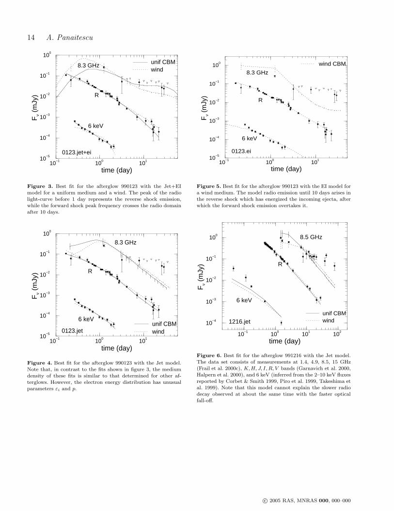
Figure 7. Best fit for the afterglow 991216 with the Jet+EImodel for a uniform medium and a wind. The addition of thereverse shock, which yields the 2 day peak of the radio emission,improves the fit to the radio data compared to that obtained withthe Jet model (figure 6).

100 101 102

time (day)

10−5

10−4

10−3

10−2

10−1

100

101

Fν

(mJy

)

unif CBMwind

0301.jo

8.5 GHz

250 GHz (x0.05)R

Figure 8. Best fit for the afterglow 000301c for the SO model.The data set contains measurements at 1.4, 4.9, 8.5, 15, 22, 100,250 350 GHz (Berger et al. 2000, Smith et al. 2001, Frail et al.2003), and K,J, I,R, V,B, U bands (Jensen et al. 2001, Rhoads& Fruchter 2001). The 250 GHz fluxes and their 2σ limits (tri-

angles) have been shifted downward by a factor 20, for clarity.Measurements between 3.0 and 4.5 days, when there is a fluc-tuation in the optical emission, have been left out. The best fitparameters for the uniform medium are given in Table 3, thosefor the wind medium are E0 = 1.5× 1053ergs sr−1, θcore = 0.9o,θobs/θcore = 2.6, q = 1.4, A∗ = 0.6, εB = 3 × 10−3, εi = 0.018,p = 2.4, AV = 0.06.

100 101 102

time (day)

10−6

10−5

10−4

10−3

10−2

10−1

100

Fν

(mJy

)

unif CBMwind0926.jo

8.5 GHz

R

0.5 keV

Figure 9. Best fit to the afterglow 000926 with the SO model.The data consists of measurements at 1.4, 4.9, 8.5, 15, 22, 99GHz (Harrison et al. 2001, Frail et al. 2003), K,H, J, I,R, V, B,Ubands (Fynbo et al. 2001, Harrison et al. 2001, Price et al. 2001),0.5 and 3 keV (inferred from the 0.2–1.5 keV and 2–10 keV fluxesreported by Harrison et al. 2001 and Piro et al. 2001).

10−1 100 101 102

time (day)

10−6

10−5

10−4

10−3

10−2

10−1

100

F ν (m

Jy)

unif CBMwind

0222.jet

8.5GHz

R

5keV

Figure 10. Best fit to the afterglow 010222 with the Jet model.The data set contains measurements at 1.4, 4.9, 8.5, 15, 22 GHz(Galama et al. 2003), K,J, I,R, V, B,U bands (Masetti et al.2001, Stanek et al. 2001), and 5 keV (inferred from the 2-10 keV

fluxes reported by in’t Zand et al. 2001). The steep X-ray fall-offafter 2 days for a wind medium is due to a high energy cutoff ofthe electron distribution, corresponding to a total electron energyof 50 per cent of the post-shock energy.

c© 2005 RAS, MNRAS 000, 000–000

16 A. Panaitescu

10−1 100 101 102

time (day)

10−6

10−5

10−4

10−3

10−2

10−1

100

F ν (m

Jy)

unif CBMwind

0222.jet+ei

8.5 GHz

R

5 keV

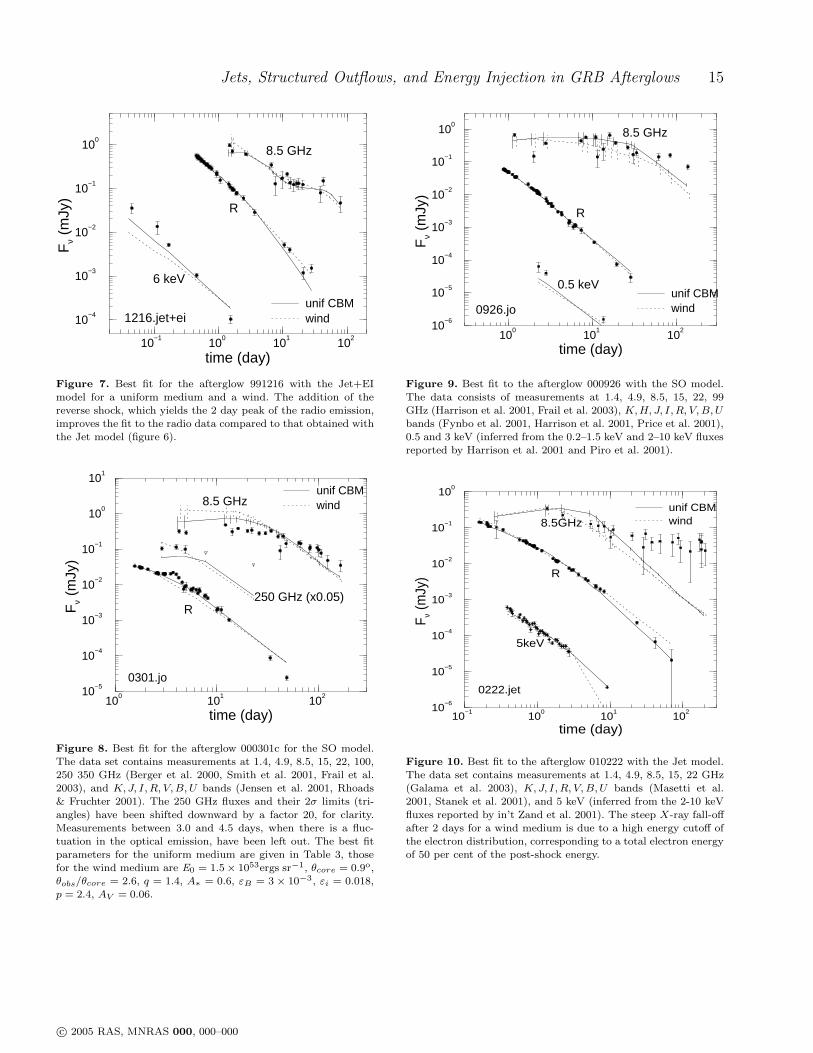
Figure 11. Best fit for the afterglow 010222 with the Jet+EImodel. For a uniform medium the forward shock component ac-commodates better the radio data after 10 days than for a wind.The 1 day hump in the radio light-curve is the reverse shock emis-sion, the forward shock overtaking at 10 days.

100 101 102

time (day)

10−6

10−5

10−4

10−3

10−2

10−1

100

F ν (m

Jy)

unif CBMwind

8.5 GHz

1211.jet

2 keV

R

Figure 12. Best fit for the afterglow 011211 with the Jet model.The data set contains measurementsat 8.5, 22 GHz (http://www.aoc.nrao.edu/∼dfrail/011211.dat),K,J, I,R, V,B, U bands (Holland et al. 2002, Jakobsson et al.2003), and 2 keV (inferred from the 0.2–5 keV fluxes measuredby Borozdin & Trodolyubov 2003). The best fit parameters areE0 = 2×1052ergs sr−1, θjet = 5.5o, n = 1.0 cm−3, εB = 6×10−4,εi = 0.047, p = 2.3, AV = 0 for a uniform medium andE0 = 4 × 1052ergs sr−1, θjet = 4.0o, A∗ = 0.6, εB = 5 × 10−4,εi = 0.030, p = 2.2, AV = 0 for a wind.

100 101 102

time (day)

10−6

10−5

10−4

10−3

10−2

10−1

100

F ν (m

Jy)

unif CBMwind8.5 GHz

1211.jo

2 keV

R

Figure 13. Best fit for the afterglow 011211 with the SO model.The best fit parameters for the uniform medium are given inTable 3, those for the wind medium are E0 = 1.2×1053ergs sr−1,θcore = 0.9o, θobs/θcore = 3.0, q = 2.3, A∗ = 0.7, εB = 10−3,εi = 0.0081, p = 2.3, AV = 0.

10−1 100 101 102

time (day)

10−4

10−3

10−2

10−1

100

Fν (

mJy

)

unif CBMwind0813.jet

8.5 GHz

2 keV

R

Figure 14. Best fit for the afterglow 020813 with theJet model. The data set contains measurements at 4.5,8.5 (http://www.aoc.nrao.edu/∼dfrail/grb020813.dat), 250 GHz(Bertoldi et al. 2002), K,H, J, I,R, V,B, U bands (Covino et al.2003, Gorosabel et al. 2004), and 2 keV (inferred from the 0.6–6keV fluxes measured by Butler et al. 2003). For the latter, thesharp steepening of the X-ray light-curve at >∼ 1 day is due tothe electron high-energy cut-off.

c© 2005 RAS, MNRAS 000, 000–000

Jets, Structured Outflows, and Energy Injection in GRB Afterglows 17

10−1 100 101 102

time (day)

10−4

10−3

10−2

10−1

100

Fν

(mJy

)

wind CBM0813.ei

8.5 GHz

2 keV

R

Figure 15. Best fit for the afterglow 020813 with the EI modelfor a wind medium. The reverse and forward shock radio emis-sions are equal at 1 day, after that the forward shock emission isstronger.

10−1 100 101

time (day)

10−6

10−5

10−4

10−3

10−2

10−1

100

Fν (

mJy

)

unif CBMwind0226.jet

8.5 GHz

2 keV

R

Figure 16. Best fit for the afterglow 030226 with theJet model. The data set contains measurements at 8.5,15, 22 GHz (http://www.aoc.nrao.edu/∼dfrail/grb030226.dat),K,H, J, I, R, V, B, U bands (Klose et al. 2004, Pandey et al.2004), and 2 keV (inferred from the 0.3–10 keV count rate re-ported by Klose et al. 2004). The best fit parameters are E0 =6 × 1052ergs sr−1, θjet = 2.8o, n = 1.6 cm−3, εB = 2 × 10−4,εi = 0.029, p = 2.2, AV = 0.09 for a uniform medium andE0 = 9 × 1052ergs sr−1, θjet = 2.6o, A∗ = 0.5, εB = 4 × 10−4,εi = 0.016, p = 2.1, AV = 0.04 for a wind.

10−1 100 101

time (day)

10−6

10−5

10−4

10−3

10−2

10−1

100

Fν (

mJy

)

unif CBMwind

0226.jo

8.5 GHz

2 keV

R

Figure 17. Best fit for the afterglow 030226 with the SO model.The best fit parameters for the uniform medium are given inTable 3, those for the wind medium are E0 = 1.3×1053ergs sr−1,θcore = 0.5o, θobs/θcore = 4.1, q = 2.8, A∗ = 0.5, εB = 6× 10−4,εi = 0.017, p = 2.2, AV = 0.03.

10−1 100 101 102 103

time (day)

10−6

10−5

10−4

10−3

10−2

10−1

100

101

Fν (

mJy

)

unif CBMwind

0508ei

8.5 GHz

R

5 keV

Figure 18. Best fit for the afterglow 970508 with the EI model.The data set contains 309 measurements at 1.4, 4.9 GHz (Frail,Waxman & Kulkarni 2000a), 86 GHz (Bremer et al. 1998),K,I, R, V, B bands (Chary et al. 1998, Galama et al. 1998, Gar-cia et al. 1998, Pedersen et al. 1998, Sahu et al. 1997, Sokolov etal. 1998), and 5 keV (inferred from 2–10 keV fluxes and spec-tral slope given in Piro et al. 1998). The fit parameters are:Ei = 9 × 1051ergs sr−1, e = 2.4, toff = 1.6 d, n = 0.9 cm−3,εB = 10−3, εi = 0.11, p = 2.3, AV = 0.15 for a uniform medium(χ2

ν = 4.5) and Ei = 7 × 1051ergs sr−1, e = 2.7, toff = 1.8 d,A∗ = 0.7 cm−3, εB = 2 × 10−2, εi = 0.063, p = 2.0, AV = 0.18for a wind (χ2

ν = 5.9).

c© 2005 RAS, MNRAS 000, 000–000